memory system evaluation for disaggregated cloud data centers
TRANSCRIPT
Memory System Evaluation for Disaggregated Cloud Data Centers
by
Andreas E. Andronikakis
A DIPLOMA THESIS
submitted to
Technical University of Crete
Presented May 8, 2017


This thesis is dedicated to my parents.For their endless love, support and
encouragement.


ABSTRACT
In our time, there is a plethora of highly demanding computational work and
of major scientific research and applications. Various ways of compressing produc-
tion costs for the above operations are also sought. There can be found a variety of
efforts to meet the above-mentioned needs such as those that promote the automa-
tion of production, those which, more generally, seek to reduce operating costs,
but simpler and less effective are those that seek to reduce non-functional costs.
Such a practice and prospect could include the development of cloud computing
and, more specifically of cloud servers, which is a necessary infrastructure for cloud
computing services to work.
Their ease of use, scalability, low cost, and reliability are some of the most im-
portant reasons for deploying cloud computing, cloud servers and their respective
service providers. One element to be highlighted is the need for a high-standard
memory in terms of performance and size. The existing architecture of Cloud
Data Centers is characterized by high energy consumption and a great waste of
resources (mainly memory).
This thesis refers to estimating the memory of cloud data centers with disag-
gregated (or disintegrated) servers, ie servers whose components and/or resources
are in separate sub-assemblies, regarding their physical location. This type of
servers is being researched over the past years, and its advantages and disad-
vantages are examined. This Disaggregated Architecture System aims to change
the traditional way of organizing a Data Center by proposing a more flexible
and software-modulated integration around blocks, the Pooled Disaggregated Re-
sources, as opposed to traditional unification around from the mainboard.
The purpose of this diploma thesis is to study and develop a unified (modular)
memory simulation tool of the above architecture, driven by the execution of an
application, the DiMEM Simulator (DIsaggregated MEMory System Simula-
tor). This simulator was implemented to approximate the behavior of standard
Cloud application workloads in Shared Architecture Memory. The tool combines
the Intel Pin Framework, where this diploma focuses, with the DRAMSim2 mem-
ory simulator.
The subject of this thesis is the study of the Dynamic Binary Instrumentation,
the understanding of Cache levels and their simulation methods, the implementa-
tion of the Disaggregated Architecture Memory simulation, and experimentation
with various parameters. The results presented approximate the overall behavior
of a Memory System of a Disaggregated Cloud Data Center.
TABLE OF CONTENTS
Page
1 Introduction . . . . . . . . . . . . . . . . . . . . . . . . . . . . . . . . . . 1
1.1 Thesis Contributions . . . . . . . . . . . . . . . . . . . . . . . . . . . 4
1.2 Thesis Outline . . . . . . . . . . . . . . . . . . . . . . . . . . . . . . . 5
2 Theoretical Background . . . . . . . . . . . . . . . . . . . . . . . . . . . 7
2.1 Instrumentation . . . . . . . . . . . . . . . . . . . . . . . . . . . . . . 82.1.1 Source Instrumentation . . . . . . . . . . . . . . . . . . . . . 92.1.2 Binary Instrumentation . . . . . . . . . . . . . . . . . . . . . 92.1.3 Dynamic Instrumentation . . . . . . . . . . . . . . . . . . . 102.1.4 Static Instrumentation . . . . . . . . . . . . . . . . . . . . . 12
2.2 Intel PIN : A Dynamic Binary Instrumentation Tool . . . . . . . . . 13
2.3 Disaggregated Architecture . . . . . . . . . . . . . . . . . . . . . . . . 182.3.1 Disaggregated System Design . . . . . . . . . . . . . . . . . 192.3.2 Replace electrons with photons . . . . . . . . . . . . . . . . 20
3 Related Work . . . . . . . . . . . . . . . . . . . . . . . . . . . . . . . . . 23
4 Implementation of DiMEM Simulator . . . . . . . . . . . . . . . . . . . . 26
4.1 Front-End of DiMEM Simulator: Instrumentation stage . . . . . . . . 264.1.1 Functional simulation of TLB and cache hierarchy using PIN 264.1.2 Instrumentation Function . . . . . . . . . . . . . . . . . . . . 314.1.3 Analysis Functions . . . . . . . . . . . . . . . . . . . . . . . 334.1.4 Instrumentation Output . . . . . . . . . . . . . . . . . . . . 364.1.5 Multithreading Functionality . . . . . . . . . . . . . . . . . . 384.1.6 Hyperthreading Functionality . . . . . . . . . . . . . . . . . 41
4.2 Back-End of DiMEM Simulator: Simulation stage . . . . . . . . . . . 42
5 Evaluation and Experimental Results . . . . . . . . . . . . . . . . . . . . 43
5.1 Evaluation . . . . . . . . . . . . . . . . . . . . . . . . . . . . . . . . . 435.1.1 CPU Metrics . . . . . . . . . . . . . . . . . . . . . . . . . . 435.1.2 DRAM Metrics . . . . . . . . . . . . . . . . . . . . . . . . . 455.1.3 Cloud Benchmarks . . . . . . . . . . . . . . . . . . . . . . . 46
5.2 Experimental Process . . . . . . . . . . . . . . . . . . . . . . . . . . . 485.2.1 Data Caching Profiling and Utilization . . . . . . . . . . . . 505.2.2 Simulation Scenarios . . . . . . . . . . . . . . . . . . . . . . 51
5.3 Experimental Results . . . . . . . . . . . . . . . . . . . . . . . . . . . 52

TABLE OF CONTENTS (Continued)
Page
5.3.1 Dense Data Caching Experimental Results . . . . . . . . . . 53
6 Conclusion and Future Work . . . . . . . . . . . . . . . . . . . . . . . . . 69
6.1 Conclusion . . . . . . . . . . . . . . . . . . . . . . . . . . . . . . . . . 69
6.2 Future Work . . . . . . . . . . . . . . . . . . . . . . . . . . . . . . . . 71
Appendices . . . . . . . . . . . . . . . . . . . . . . . . . . . . . . . . . . . . 73
A Some useful codes . . . . . . . . . . . . . . . . . . . . . . . . . . . . . 74
B Simulation output . . . . . . . . . . . . . . . . . . . . . . . . . . . . . 86
LIST OF FIGURES
Figure Page
1.1 Whole System Abstract Figure. . . . . . . . . . . . . . . . . . . . . 4
2.1 This diagram depicts a scheme pertaining to the dynamic type (DBI). 10
2.2 DBI Frameworks. . . . . . . . . . . . . . . . . . . . . . . . . . . . . 11
2.3 This diagram depicts a scheme pertaining to the dynamic type (DBI). 13
2.4 The architecture of Pin. . . . . . . . . . . . . . . . . . . . . . . . . 14
2.5 1 Trace, 2 BBLs, 6 instructions . . . . . . . . . . . . . . . . . . . . 17
2.6 Architectural differences between server-centric and resource-centricdatacenters. . . . . . . . . . . . . . . . . . . . . . . . . . . . . . . . 18
2.7 Block Diagram of high-level dReDBox Rack-scale architecture . . . 20
2.8 Disaggregated data center interconnect requirements (Courtesy ofThe Optical Society) [7] . . . . . . . . . . . . . . . . . . . . . . . . 21
4.1 The DiMEM Simulator Logo. . . . . . . . . . . . . . . . . . . . . . 26
4.2 Cache hierarchy of the K8 core in the AMD Athlon 64 CPU. . . . . 27
4.3 An example of a Multicore cache hierarchy . . . . . . . . . . . . . . 29
4.4 local.hpp File Reference . . . . . . . . . . . . . . . . . . . . . . . . 30
4.5 Front-End Diagram . . . . . . . . . . . . . . . . . . . . . . . . . . . 31
4.6 Analysis Function . . . . . . . . . . . . . . . . . . . . . . . . . . . . 33
5.1 DataCaching Power8 workload analysis. . . . . . . . . . . . . . . . . 51
5.2 Power 8 DataCaching 2GB Results . . . . . . . . . . . . . . . . . . 54
5.3 Cortex-A53 DataCaching 2GB Results . . . . . . . . . . . . . . . . 55
5.4 Cortex-A57 DataCaching 2GB Results . . . . . . . . . . . . . . . . 56
5.5 Power 8 DataCaching 4GB Results . . . . . . . . . . . . . . . . . . 57
5.6 Cortex-A53 DataCaching 4GB Results . . . . . . . . . . . . . . . . 58
5.7 Cortex-A57 DataCaching 4GB Results . . . . . . . . . . . . . . . . 59

LIST OF FIGURES (Continued)
Figure Page
5.8 Power 8 DataCaching 8GB Results . . . . . . . . . . . . . . . . . . 60
5.9 Cortex-A53 DataCaching 8GB Results . . . . . . . . . . . . . . . . 61
5.10 Cortex-A57 DataCaching 8GB Results . . . . . . . . . . . . . . . . 62
5.11 Power 8 DataCaching 16GB Results . . . . . . . . . . . . . . . . . . 63
5.12 Cortex-A53 DataCaching 16GB Results . . . . . . . . . . . . . . . . 64
5.13 Cortex-A57 DataCaching 16GB Results . . . . . . . . . . . . . . . . 65
5.14 Power 8 DataCaching 32GB Results . . . . . . . . . . . . . . . . . . 66
5.15 Cortex-A53 DataCaching 32GB Results . . . . . . . . . . . . . . . . 67
5.16 Cortex-A57 DataCaching 32GB Results . . . . . . . . . . . . . . . . 68
LIST OF TABLES
Table Page
4.1 Multithreading example . . . . . . . . . . . . . . . . . . . . . . . . 41
5.1 CPU table 1 . . . . . . . . . . . . . . . . . . . . . . . . . . . . . . . 44
5.2 ARM Cortex-A53 Cache Metrics . . . . . . . . . . . . . . . . . . . 44
5.3 ARM Cortex-A57 Cache Metrics . . . . . . . . . . . . . . . . . . . 44
5.4 IBM Power8 Cache Metrics . . . . . . . . . . . . . . . . . . . . . . 44
5.5 DRAM Metrics - Modified DDR4 Micron 1G 16B x4 sg083E . . . . 45
5.6 Nanosecond to Memory Cycles Disaggregated Latency Correspon-dence . . . . . . . . . . . . . . . . . . . . . . . . . . . . . . . . . . . 52

CHAPTER1Introduction
”We believe we’re moving out of the Ice Age, the Iron
Age, the Industrial Age, the Information Age, to the
participation age. (...) You are participating on the
Internet, not just viewing stuff. We build the
infrastructure that goes in the data center that
facilitates the participation age.”
— Scott McNealy, former CEO, Sun Microsystems
Cloud computing is where software applications, data storage and processing
capacity are accessed from a cloud of online resources. This permits individual
users to access their data and applications from any device, as well as, allowing
organizations to reduce their capital costs by producing software and hardware as
a utility service[9]. Cloud computing is closely associated with Web 2.0.
These times, as was in the past, organizations, institutes, even legal entities
engage in the business and production sector, looking for various ways to boost
output, improve productivity and compress production costs. One can find diverse
efforts, such as those that promote the automation of production; in general, they
seek to reduce operating costs, but being simpler and with less impact than those
1. INTRODUCTION 2
that seek to reduce non-recurring costs. The development of cloud computing
could be included in such a producting practice and perspective, as well as, more
specifically, cloud servers, which consist a necessary infrastructure enabling one to
operate the cloud computer services. This is a booming field that has attracted
providers like Microsoft and Amazon, which have developed Microsoft Azure and
Amazon Web Services (AWS), respectively. The main services offered are the IaaS
(Infrastructure as a Service), PaaS (Platform as a Service), SaaS (Software as a
Service), i.e. infrastructure services, platform and software[4].
One issue that arises is the specific booming and growth causes in cloud com-
puting over the past years, with greater emphasis on those from 2009 onwards.
The thesis will list and analyze some of the most fundamental ones below[4]:
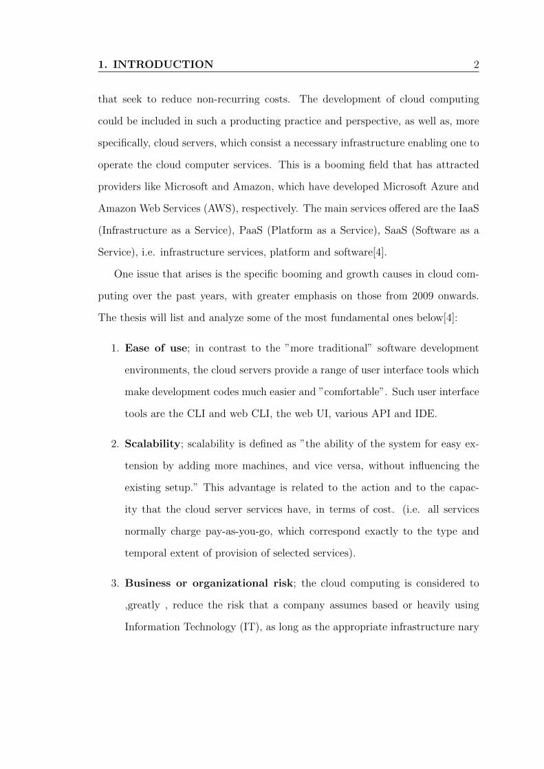
1. Ease of use; in contrast to the ”more traditional” software development
environments, the cloud servers provide a range of user interface tools which
make development codes much easier and ”comfortable”. Such user interface
tools are the CLI and web CLI, the web UI, various API and IDE.
2. Scalability; scalability is defined as ”the ability of the system for easy ex-
tension by adding more machines, and vice versa, without influencing the
existing setup.” This advantage is related to the action and to the capac-
ity that the cloud server services have, in terms of cost. (i.e. all services
normally charge pay-as-you-go, which correspond exactly to the type and
temporal extent of provision of selected services).
3. Business or organizational risk; the cloud computing is considered to
,greatly , reduce the risk that a company assumes based or heavily using
Information Technology (IT), as long as the appropriate infrastructure nary
3
fixed costs of the business, due to the coverage of the need for computing
infrastructure through the cloud.
4. Cost; as mentioned above, similar service providers through cloud servers
correspond exactly to the demand required by each specific customer, while
the burden is only on the basis of accurate computational power and time
use of specific computing resources. Given that, the potential for cloud
computing services to the type, quantity and time, required one need to be
of no capital expense texture but only of functional. At the same time, there
is no need for maintenance of servers or software, and therefore thus, the
total cost of the organization or undertaking is reduced.
5. Reliability; is a key element that justifies the development of cloud com-
puting and, for some, it is a primary key element. What is indicated in these
cases is that storing data in a portable storage medium such as a USB Stick
disk or CD / DVD is a less reliable solution than storing them in a cloud
computing service, such as, for example, Rapidshare, Mega or the Dropbox.
All the above explains the development of cloud computing, the cloud server
and the respective service providers. One point that should be emphasized in this
introduction is the need for a high standard memory. An explanation given to
the urgency of the existence of this element from the inside to the lowest extent
is that Cloud Computing services (IaaS) meet virtual memory services, as well.
But an even more important issue has to do with the fact that cloud computing
services are memory intensive. In other words, such an architecture (and amount)
of memory is required, which permits the expansion of services to a sufficient
degree for each customer. This implies that the important advantage of scalability
1. INTRODUCTION 4
is based on such adequacy of memory in all species. The same applies to the cache,
the channels and broadband[9].
1.1 Thesis Contributions
This thesis relates to the judgment of the memory of cloud data centers with
disaggregated (or disintegrated) servers, in other words servers whose ingredients
or resources are in separate -concerning the physical location- subsystems[17, 32,
16, 23]. This type of servers has been under research lately, and the advantages
and disadvantages are presented. The reason for using cloud computing is that it
offers a better exploitation of the resources. In chapter 2 of this thesis, we will
make extensive reference to the theoretical background of that architecture.
In this thesis the design and implementation of a complete Memory System
Simulator is presented, as well as, the memory system evaluation of disaggregated
cloud data centers.
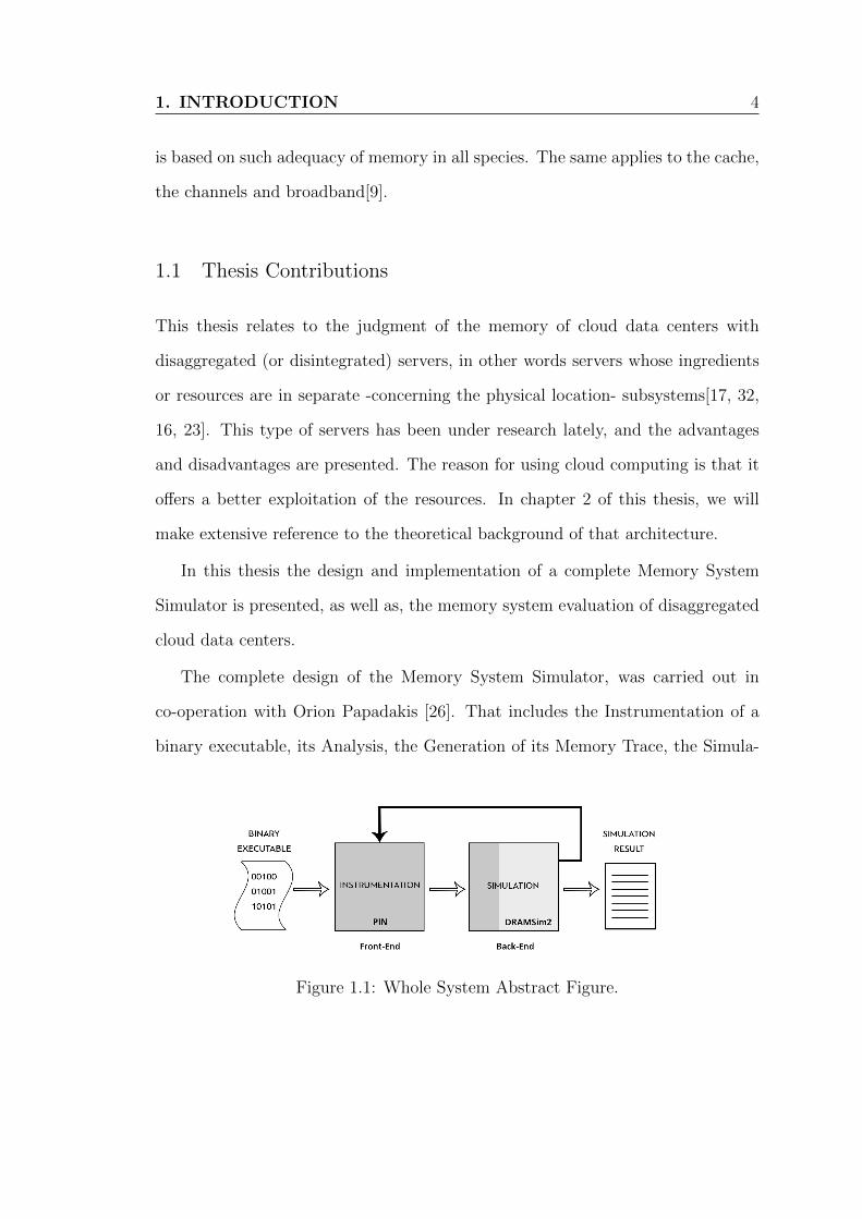
The complete design of the Memory System Simulator, was carried out in
co-operation with Orion Papadakis [26]. That includes the Instrumentation of a
binary executable, its Analysis, the Generation of its Memory Trace, the Simula-
Figure 1.1: Whole System Abstract Figure.
5 1.2 Thesis Outline
tion of that Trace and the Exertion of Final Results. The Simulator was based on
DRAMSim2[28], a Cycle Accurate Memory System Simulator for modelling and
simulation, as the back-end, while the front-end driver was developed from scratch.
The current thesis focuses on the front-end driver of our Simulator. In order
to implement that, we have created a tool, using Intel’s PIN[27, 22], a dynamic
binary instrumentation framework. Our PINtool simulates the functionality of all
Cache and TLB levels (of a given CPU-model) and generates a Trace File with
all RAM Accesses, including their Type of Access(Read/Write) and their Clock
Cycle. That Trace File is necessary for the back-end of the Simulator, which was
implemented by Orion Papadakis. To achieve the pairing between front-end and
back-end, DRAMSim2 was included, as a library on our PINtool, in order to export
the final .log file with the Simulation Results.
Our Simulator has been designed to be used on Disaggregated Cloud Servers,
in order to, effectively, draw conclusions about their Memory Usage on different
scenarios, by changing the Disaggregated/Local Memory Percentage.
1.2 Thesis Outline
In Chapter 2 we provide the theoretical background needed in order for the reader
to comprehend the need of an efficient Cloud Computing Memory System and also
the way to do the Instrumentation. All four forms of Instrumentation, and their
combinations, are presented and so is the Intel PIN framework, the tool used for the
Cloud Server’s Instrumentation. Finally, we present the theoretical background of
the Disaggregated Architectures. In Chapter 3 of this thesis, we present the related
work done in the field of Memory Simulation, using Instrumentation tools, as well
1. INTRODUCTION 6
as, research about Disaggregated Cloud Data Centers. In Chapter 4 we present
the complete Design of our Simulator, describing, in detail, all steps of it.
Consequently, Chapter 5 contains the results derived from the Simulations
made by our tool. We have used Cloudsuite Benchmarks, for our Simulations,
in order to evaluate the performance and efficiency of the cloud services to be
assessed, also considering some different Disaggregated Architectures. Finally,
Chapter 6 concludes the thesis and provides comments for possible future work.
In Appendix A the reader will find some useful codes that refer to different points
of the thesis.
CHAPTER2Theoretical Background
This thesis identifies three specific restrictive elements concerning Cloud Comput-
ing; three restrictions which are imported because of the way current data centers
are built. These are [17]:
• The proportionality of the resources of the entire system follows that of the
mainboard (basic building block). Thus, it is not possible to focus on certain
elements that are crucial priorities, such as memory, so each system upgrades
should involve all elements, as they existed in its first manufacturing and
assembly.
• There is inadequate allocation of computing resources because of their con-
centration in one spot and their endorsement as a compact whole. The com-
putational processing resources (CPU cores) can be fully exploited, while,
conversely, utilizing only a relatively small amount of memory. Concentra-
tion of the cloud server components in a system thereby, leads to a fragmen-
tation and great inefficiencies of their resources.
• Even when a single cloud server component is upgraded, the entire system
of the server board is affected. Conversely, a disaggregated cloud server’s
2. THEORETICAL BACKGROUND 8
component could, with great discretion, be upgraded.
In order to solve these problems, the disaggregation or disintegration (frag-
mentation) of cloud servers was invented[17, 20, 21, 32]. However, as mentioned
above, there are some critical elements of cloud computing necessary to operate
with completeness in the above objectives. The prerequisite to do this is the in-
stallation and operation of specific control methods in the code source and binary
form. One of these ways will be analyzed in all its forms in this chapter. Specif-
ically, four of the main types of “orchestration code” as it is often called, will be
referred to. These are binary, source, dynamic and static instrumentation code.
2.1 Instrumentation
The instrumentation is a specific term used to denote the process and technique
of use and adding a control code that interferes with an intercalary way in a
program or the programming environment, in order to monitor or modify any
program behavior[8]. This technique proves very useful nowadays, since there are
a number of problems associated with the development of a code, which can, then,
be identified and eliminated. Thus, some of the objectives of the instrumentation
code can be:
• Gathering metrics code values.
• Automated debugging code.
• Detection (of other) error code.
• Memory Leak Detection.
9 2.1 Instrumentation
The general form of the process of instrumentation of the code also includes some
basic steps applicable to all sub. These are:
1. Determination of the points where the instrumentation will be implemented.
2. Introduction and implementation of specific form of the instrumentation
code.
3. Taking up the control of the program (compiler / linker, etc.).
4. Saving the program execution parameters.
5. Execution of the Control Code (instrumentation).
6. Restoration of the pre-existing program execution parameters.
7. Returning the control to the main program.
2.1.1 Source Instrumentation
The first type of instrumentation code to which we will refer to, is the source code
instrumentation[11]. The special feature of this format is that instrumentation
applies to the source code, which is written and performed at the level used in this
codes programming language.
2.1.2 Binary Instrumentation
Binary (or bytecode) instrumentation has to do with the binary code[2]. That is,
its basic difference, regarding the other types of instrumentation and especially
2. THEORETICAL BACKGROUND 10
source instrumentation, is that it refers to the microprogramming/assembly form
of the code, somewhere between the source and the machine code and, in fact,
one level above the latter. The binary instrumentation which is often used, is the
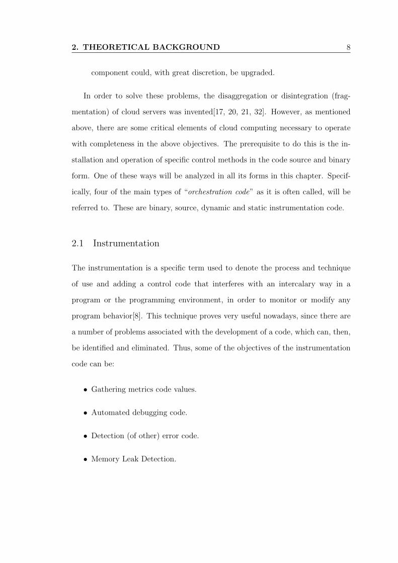
dynamic binary instrumentation, but there is the static one as well[5]. The diagram
below depicts a scheme pertaining to the dynamic type (DBI) (Figure 2.3).
Figure 2.1: This diagram depicts a scheme pertaining to the dynamic type (DBI).
We will refer to DBI, as well as to the additional aforementioned terms, in the
subsequent paragraphs.
2.1.3 Dynamic Instrumentation
Dynamic instrumentation is a more specific technique which is an important and
very frequently used element within the broader framework of instrumentation
techniques. Binary instrumentation is the most usual context of binary instru-
mentation, thus formulating dynamic binary instrumentation or Dynamic Binary
Instrumentation (DBI). The most distinctive characteristic of DBI is that the in-
strumentation process takes place shortly before it is executed. As a consequence,
11 2.1 Instrumentation
recompilation or re-linking of the code is not indispensable, as in the static one, as
will be seen in the forthcoming paragraph. This concept is named as Just In Time
or JIT[5] . The code is actually attached to processes already being executed,
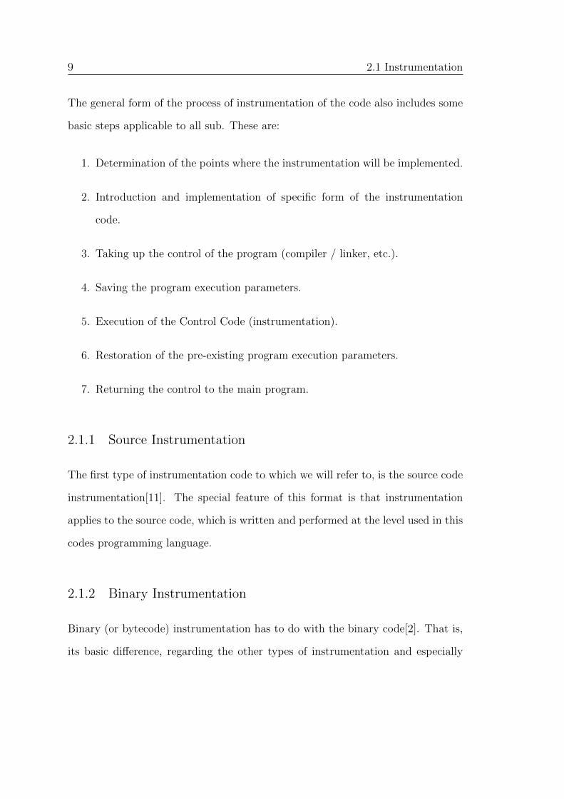
hence the DBI code is considered to be injected into the whole code corpus. DBI
is implemented by tools such as PIN[27, 22], DynamoRIO[3, 30], DynInst[29] and
Valgrind[24].
Frameworks OS Arch Modes Features
PIN
Linux,
Windows,
MacOS
x86, x86-64,
Itanium, ARMJIT, Probe Attach mode
DynamoRIOLinux,
Windowsx86, x86-64 JIT, Probe
Runtime
optimization
DynInst
Linux,
FreeBSD,
Windows
x86, x86-64,
ppc32, ARM,
PPC64
Probe
Static & Dynamic
binary
instrumentation
Valgrind Linux, MacOS
x86, x86-64,
ppc32, ARM,
PPC64
JIT
IR-VEX,
Heavyweight DBA
tools
Figure 2.2: DBI Frameworks.
There are two kinds of DBI tools in all:
• Instrumentation code parts. The instrumentation parts are injected just
before a specific instruction which exists for the first time and defines the
place that instrumentation is implemented.
• Analysis code parts. The analysis code parts are inserted each time an in-
struction is met and define the specific instrumentation functionalities which
are to be implemented in the code.

2. THEORETICAL BACKGROUND 12
Pros & Cons: start-up times are much slower and the demand of memory usage
is increased as each method body has to be reallocated. The same applies to the
CPU load to instrument on the fly.
Dynamic analysis implies capability to administer code which is generated in
a dynamic or self-modifying manner.
2.1.4 Static Instrumentation
Static instrumentation appears, as the dynamic one, in the context of binary in-
strumentation. Thus, static binary instrumentation has got certain attributes
according to which it functions. The basic elements which differentiate it from
the dynamic type is that there are additional parts of code which are included
beforehand (not “Just In Time”), namely a segment and data. An other differ-
ence is that the instrumentation occurs before even the program starts running.
Furthermore, the header may be edited, as the following image indicates. The
important thing is that the probes are baked inside the binary. This can be done
in two ways:
First by having the compiler put the probes in.[15] Second, by what is called
post link instrumentation. This gives immediate access to all the methods and
instruments included in the binary and makes all the necessary changes.
Pros & Cons: This approach accomplishes much faster start-up times, since
the images are loaded in to memory are the image that run.

13 2.2 Intel PIN : A Dynamic Binary Instrumentation Tool
Figure 2.3: This diagram depicts a scheme pertaining to the dynamic type (DBI).
2.2 Intel PIN : A Dynamic Binary Instrumentation Tool
Pin is a framework for dynamic binary instrumentation[27, 22]. It supports the
Android, Linux, OS X and Windows operating systems and executables for the
IA-32, Intel(R) 64 and Intel(R) Many Integrated Core architectures.
The functionality of this framework is the insertion of an arbitrary code (written
in C or C++) in arbitrary places in the executable. While the executable is
running, the code is added dynamically, something that also makes the attachment
of the Pin to an already running process, possible.
“Pin provides a rich API that abstracts away the underlying instruction set id-
iosyncrasies and allows context information such as register contents to be passed
to the injected code as parameters. Pin automatically saves and restores the regis-
ters that are overwritten by the injected code so the application continues to work.
Limited access to symbol and debug information is available as well.” as described
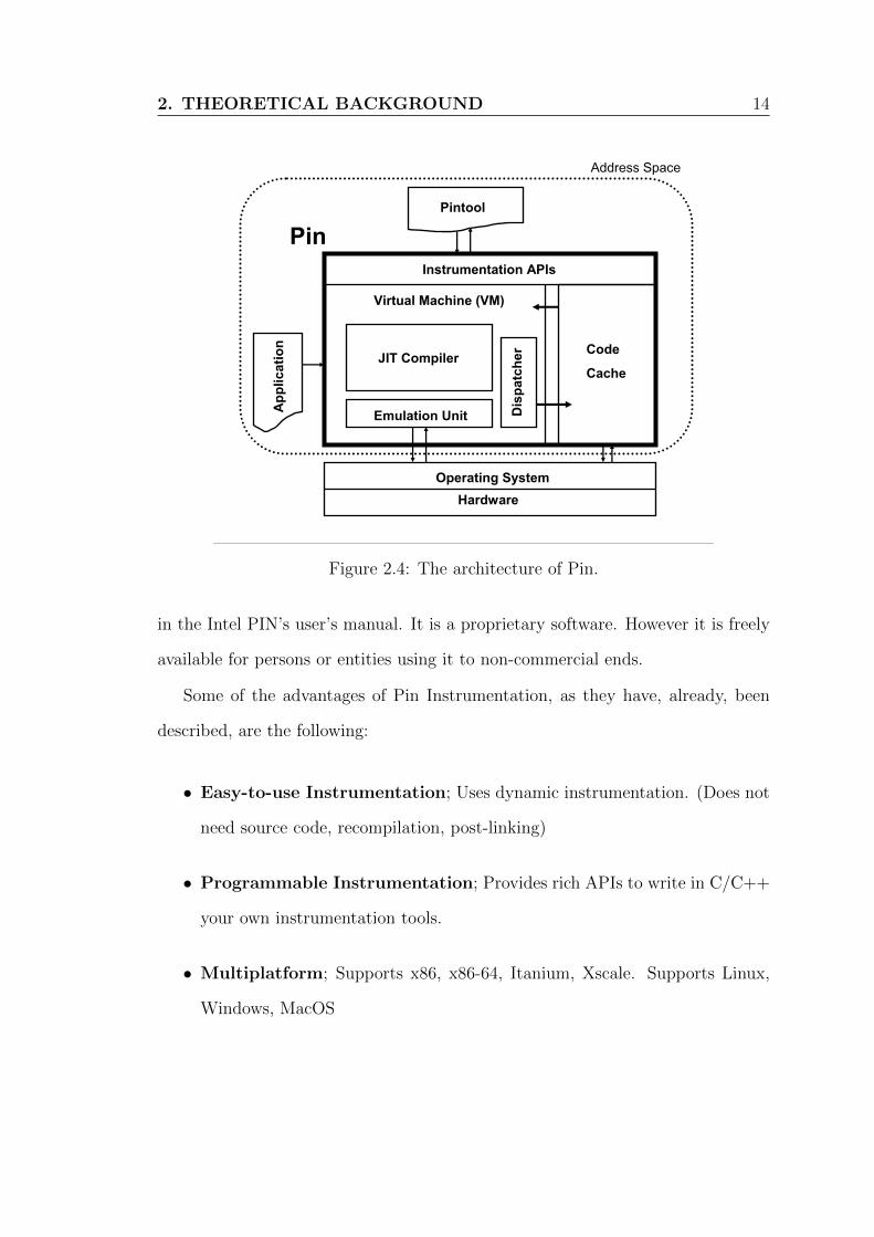
2. THEORETICAL BACKGROUND 14
JIT Compiler
Emulation Unit Dis
patc
her
Virtual Machine (VM)
Code
Cache
Instrumentation APIsA
pp
lic
ati
on
Operating System
Hardware
Pin
Pintool
Address Space
Figure 2. Pin’s software architecture
mentation API invoked by Pintools. The VM consists of a just-in-time compiler (JIT), an emulator, and a dispatcher. After Pin gainscontrol of the application, the VM coordinates its components toexecute the application. The JIT compiles and instruments applica-tion code, which is then launched by the dispatcher. The compiledcode is stored in the code cache. Entering/leaving the VM from/tothe code cache involves saving and restoring the application registerstate. The emulator interprets instructions that cannot be executeddirectly. It is used for system calls which require special handlingfrom the VM. Since Pin sits above the operating system, it can onlycapture user-level code.
As Figure 2 shows, there are three binary programs presentwhen an instrumented program is running: the application, Pin, andthe Pintool. Pin is the engine that jits and instruments the applica-tion. The Pintool contains the instrumentation and analysis routinesand is linked with a library that allows it to communicate with Pin.While they share the same address space, they do not share any li-braries and so there are typically three copies of glibc. By makingall of the libraries private, we avoid unwanted interaction betweenPin, the Pintool, and the application. One example of a problematicinteraction is when the application executes a glibc function thatis not reentrant. If the application starts executing the function andthen tries to execute some code that triggers further compilation, itwill enter the JIT. If the JIT executes the same glibc function, itwill enter the same procedure a second time while the applicationis still executing it, causing an error. Since we have separate copiesof glibc for each component, Pin and the application do not shareany data and cannot have a re-entrancy problem. The same prob-lem can occur when we jit the analysis code in the Pintool thatcalls glibc (jitting the analysis routine allows us to greatly reducethe overhead of simple instrumentation on Itanium).
3.2 Injecting Pin
The injector loads Pin into the address space of an application. In-jection uses the Unix Ptrace API to obtain control of an applicationand capture the processor context. It loads the Pin binary into theapplication address space and starts it running. After initializingitself, Pin loads the Pintool into the address space and starts it run-ning. The Pintool initializes itself and then requests that Pin startthe application. Pin creates the initial context and starts jitting theapplication at the entry point (or at the current PC in the case ofattach). Using Ptrace as the mechanism for injection allows us toattach to an already running process in the same way as a debug-ger. It is also possible to detach from an instrumented process andcontinue executing the original, uninstrumented code.
Other tools like DynamoRIO [6] rely on the LD PRELOAD en-vironment variable to force the dynamic loader to load a shared li-brary in the address space. Pin’s method has three advantages. First,LD PRELOAD does not work with statically-linked binaries, whichmany of our users require. Second, loading an extra shared librarywill shift all of the application shared libraries and some dynami-cally allocated memory to a higher address when compared to anuninstrumented execution. We attempt to preserve the original be-havior as much as possible. Third, the instrumentation tool cannotgain control of the application until after the shared-library loaderhas partially executed, while our method is able to instrument thevery first instruction in the program. This capability actually ex-posed a bug in the Linux shared-library loader, resulting from areference to uninitialized data on the stack.
3.3 The JIT Compiler
3.3.1 Basics
Pin compiles from one ISA directly into the same ISA (e.g., IA32to IA32, ARM to ARM) without going through an intermediateformat, and the compiled code is stored in a software-based codecache. Only code residing in the code cache is executed—the origi-nal code is never executed. An application is compiled one trace ata time. A trace is a straight-line sequence of instructions which ter-minates at one of the conditions: (i) an unconditional control trans-fer (branch, call, or return), (ii) a pre-defined number of conditionalcontrol transfers, or (iii) a pre-defined number of instructions havebeen fetched in the trace. In addition to the last exit, a trace mayhave multiple side-exits (the conditional control transfers). Eachexit initially branches to a stub, which re-directs the control to theVM. The VM determines the target address (which is statically un-known for indirect control transfers), generates a new trace for thetarget if it has not been generated before, and resumes the executionat the target trace.
In the rest of this section, we discuss the following features ofour JIT: trace linking, register re-reallocation, and instrumentationoptimization. Our current performance effort is focusing on IA32,EM64T, and Itanium, which have all these features implemented.While the ARM version of Pin is fully functional, some of theoptimizations are not yet implemented.
3.3.2 Trace Linking
To improve performance, Pin attempts to branch directly from atrace exit to the target trace, bypassing the stub and VM. Wecall this process trace linking. Linking a direct control transferis straightforward as it has a unique target. We simply patch thebranch at the end of one trace to jump to the target trace. However,an indirect control transfer (a jump, call, or return) has multiplepossible targets and therefore needs some sort of target-predictionmechanism.
Figure 3(a) illustrates our indirect linking approach as imple-mented on the x86 architecture. Pin translates the indirect jumpinto a move and a direct jump. The move puts the indirect targetaddress into register %edx (this register as well as the %ecx and%esi shown in Figure 3(a) are obtained via register re-allocation,as we will discuss in Section 3.3.3). The direct jump goes to thefirst predicted target address 0x40001000 (which is mapped to0x70001000 in the code cache for this example). We compare%edx against 0x40001000 using the lea/jecxz idiom used in Dy-namoRIO [6], which avoids modifying the conditional flags reg-ister eflags. If the prediction is correct (i.e. %ecx=0), we willbranch to match1 to execute the remaining code of the predictedtarget. If the prediction is wrong, we will try another predicted tar-get 0x40002000 (mapped to 0x70002000 in the code cache). If thetarget is not found on the chain, we will branch to LookupHtab 1,which searches for the target in a hash table (whose base address is
192
Figure 2.4: The architecture of Pin.
in the Intel PIN’s user’s manual. It is a proprietary software. However it is freely
available for persons or entities using it to non-commercial ends.
Some of the advantages of Pin Instrumentation, as they have, already, been
described, are the following:
• Easy-to-use Instrumentation; Uses dynamic instrumentation. (Does not
need source code, recompilation, post-linking)
• Programmable Instrumentation; Provides rich APIs to write in C/C++
your own instrumentation tools.
• Multiplatform; Supports x86, x86-64, Itanium, Xscale. Supports Linux,
Windows, MacOS

15 2.2 Intel PIN : A Dynamic Binary Instrumentation Tool
• Robust; Instruments real-life applications: Database, web browsers, Instru-
ments multithreaded applications, Supports signals
• Efficient; Applies compiler optimizations on instrumentation code
Pin includes the source code for a large number of example instrumentation
tools, like basic block profilers, cache simulators, instruction trace generators, etc.
It is easy to derive new tools using the examples as a template.
The PIN engine uses the so-called PIN tools, for example an Instruction Count-
ing Tool. The two main components of a Pin tool are: instrumentation and
analysis routines:
• The Instrumentation routine’s role is to insert calls to user defined analysis
routines, by utilizing the rich API provided by Pin. These calls are inserted
at arbitrary points in the application instruction stream. The basic charac-
teristics of an application to instrument, are defined by the instrumentation
routines.
• Analysis routines are called by the instrumentation routines at application
run time.
For example, a user can write an instrumentation routine that instruments
every instruction executed by an application via the Pin API [4]. This Pintool
can count the total number of dynamic instructions executed by the program,
once the instrumentation routine sets up a call to the user-defined analysis routine
DoCount() (which increments a counter)
Moreover, Intel’s PIN provides further advanced features, helpful in a variety
of microarchitecture studies.

2. THEORETICAL BACKGROUND 16
For example, pintools can:
• profile the dynamic or static distribution of instructions executed by a given
application.
• acquire effective addresses of all memory instructions executed.
• determine the outcomes of branch instructions and their associated branch
targets.
• change architectural state of registers.
All the above information provides users with customizable Pintools which
model branch predictors, simple performance models and cache simulators.
Some of the basic arguments through which it is determined how instrumenta-
tion is carried out, are the following:
• IPOINT_BEFORE: a call is inserted before an instruction or a routine.
• IPOINT_AFTER: a call is inserted at the final paths of an instruction or a
routine.
• IPOINT_ANYWHERE: an instrumentation call is made anywhere within the ad-
ditional code corpus(that is, in a trace the PIN callback-function or a bbl).
• IPOINT_TAKEN_BRANCH: an instrumentation call is inserted on the taken edge
of a branch, given that all the proper alterations are made.
An example code which includes such an argument is the following:
17 2.2 Intel PIN : A Dynamic Binary Instrumentation Tool
1 void I n s t r u c t i o n ( INS ins , void ∗v )2 {3 INS In s e r tCa l l ( ins , IPOINT BEFORE,4 (AFUNPTR) docount , IARG END) ;5 }
Listing 2.1: An example of Instruction() function
Let it be noted here, that the PIN is initiated through the use of the following
instruction: PIN_Init(argc, argv); Subsequently, in order to perform the instru-
mentation for the next instruction encountered, PIN uses the elements analyzed
below:
1. The Function by the name Instruction().
2. The function INS_InsertCall(). This function takes, among others, the
arguments’ values specified above, as acceptable values for its second argu-
ment.
3. The function Fini(). This function is called when the application is about
to exit the program .
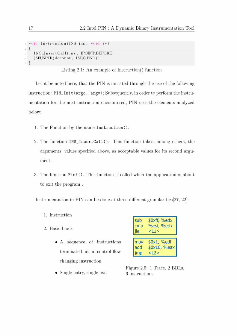
Instrumentation in PIN can be done at three different granularities[27, 22]:
1. Instruction
2. Basic block
• A sequence of instructions
terminated at a control-flow
changing instruction
• Single entry, single exitFigure 2.5: 1 Trace, 2 BBLs,6 instructions
2. THEORETICAL BACKGROUND 18
3. Trace
• A sequence of basic blocks terminated at an unconditional control-flow
changing instruction
• Single entry, multiple exits
Every PIN tool performs different tasks to the instructions of the instrumented
program, and for every task there is a different function which implements it. For
example, the functions docount() or printip() are utilized, in order to perform
instruction counting or related IP printing. The same rules apply to the rest of
the PIN tools of the PIN engine.
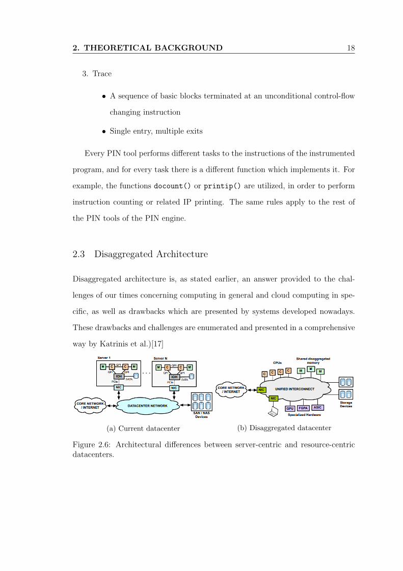
2.3 Disaggregated Architecture
Disaggregated architecture is, as stated earlier, an answer provided to the chal-
lenges of our times concerning computing in general and cloud computing in spe-
cific, as well as drawbacks which are presented by systems developed nowadays.
These drawbacks and challenges are enumerated and presented in a comprehensive
way by Katrinis et al.)[17]
(a) Current datacenter (b) Disaggregated datacenter
Figure 2.6: Architectural differences between server-centric and resource-centricdatacenters.
19 2.3 Disaggregated Architecture
2.3.1 Disaggregated System Design
Disaggregation, by definition, means “separation into components”. Disaggregated
(or disintegrated) systems are systems which have components spread across sev-
eral physical locations. These systems are in a position to address certain issues of
paramount importance, such as scalability and (modular) heterogeneity[12]. This
type of architecture seems to introduce certain new challenges, such as, the need to
diminish a new overhead which appears, due to new forms of latency, which show
up in the architecture. However, it is the advantages of this architecture that
outweigh its disadvantages. One of the main goals of disintegrated architectures
is to promote and elevate the utilization degree of each component of a server or
data center. Such components are the ones pertaining to memory, (central, graph-
ical etc.) processing units, acceleration and storage units. It has been noted that
due to the integration of all these components into concrete computing units and
servers, there can be a massive -larger than 50%- underutilization. Every upgrade,
on the other hand, has to see these systems as a whole. Disintegration reverses
this process, which ceases to exist; it offers a much greater degree of flexibility, so
that the redundancy of systems hardware and the associated costs are significantly
lowered in a cost-effective way.
Especially, it is the memory quantity, quality and cost that have, long, been
a difficult problem to process and solve. As described above, it is especially the
cloud computing applications which are memory-intensive, thus they require a
more centered approach. It seems that the disintegrated architecture is able to
tackle this issue in a very efficient way. The issues solved[12] are the ones described
above, through the separate management and upgrade of each component.
2. THEORETICAL BACKGROUND 20
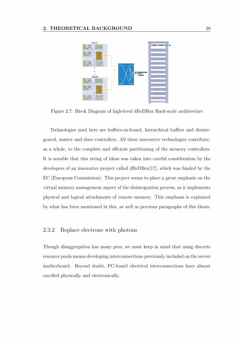
Figure 2.7: Block Diagram of high-level dReDBox Rack-scale architecture
Technologies used here are buffers-on-board, hierarchical buffers and disinte-
grated, master and slave controllers. All these innovative technologies contribute,
as a whole, to the complete and efficient partitioning of the memory controllers.
It is notable that this string of ideas was taken into careful consideration by the
developers of an innovative project called dReDBox[17], which was funded by the
EC (European Commission). This project seems to place a great emphasis on the
virtual memory management aspect of the disintegration process, as it implements
physical and logical attachments of remote memory. This emphasis is explained
by what has been mentioned in this, as well as previous paragraphs of this thesis.
2.3.2 Replace electrons with photons
Though disaggregation has many pros, we must keep in mind that using discrete
resource pools means developing interconnections previously included on the server
motherboard. Beyond doubt, PC-board electrical interconnections have almost
excelled physically and electronically.
21 2.3 Disaggregated Architecture
The answer may lie in the science of photonics. Photonics are defined as “a
research field whose goal is to use light to perform functions that traditionally fell
within the typical domain of electronics such as telecommunications and informa-
tion processing.”
Photons are already used to disseminate traffic from data center racks to the
rest of the digital world. Researchers are finding ways to replace electrical signals
all the way to the processor silicon, which raises the question of the use of fiber-
optic runs to interconnect the resource pools.
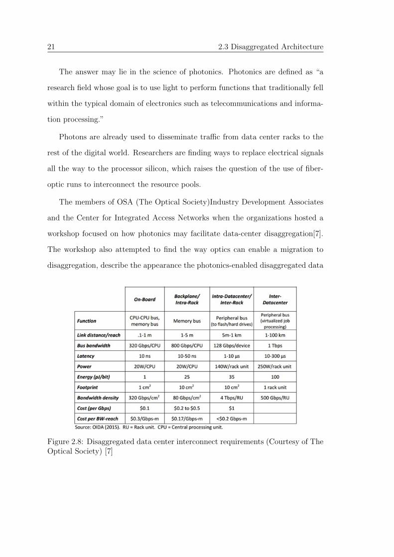
The members of OSA (The Optical Society)Industry Development Associates
and the Center for Integrated Access Networks when the organizations hosted a
workshop focused on how photonics may facilitate data-center disaggregation[7].
The workshop also attempted to find the way optics can enable a migration to
disaggregation, describe the appearance the photonics-enabled disaggregated data
Figure 2.8: Disaggregated data center interconnect requirements (Courtesy of TheOptical Society) [7]

2. THEORETICAL BACKGROUND 22
center and the performance metrics/requirements essential to photonics in disag-
gregated data centers
Disaggregation offers improved efficiency and increased capacity, but the ben-
efits are limited by the cost and performance of the photonic interconnections.
Latency requirements, in particular, impose hard limits on distances over which
certain resources can be disaggregated.
The workshop attendees were optimistic about fiber-optic interconnects replac-
ing electrical cables everywhere except on the rack shelf. Optics will out compete
electrical interconnects for links that enable disaggregation if optics can hit the
metrics of cost, performance, and size. The above table (Figure 2.8) lists the
aforementioned metrics.

CHAPTER3Related Work
This thesis is related to projects which span several different topics, from in-
strumentation implementation to disaggregated (disintegrated) cloud servers dis-
courses. Regarding the programming work which was carried out in this thesis,
there are a lot of similarities with certain projects. We will refer to the most
important one below, which, in a way, inspired the whole thesis.
This thesis is based on the PIN project, released by Intel in 2012[27, 22] .
PIN uses, as has been mentioned above, instrumentation and analysis routines
and is very popular, as well as very broadly used in scientific studies and publica-
tions(40.000 users, 400 scientific citations). The PIN project is the one from which
this dissertation has derived a great deal of elements, as well as its fundamental
notions and inspiration.
The work named “Ramulator: A Fast and Extensible DRAM Simulator”[18]
is one similar to ours, fundamentally in terms of its DRAM usage and simulator.
The authors contribute their own version of a DRAM simulator, which empha-
sizes strongly on the concept of extensibility. Ramulator is based on a modular
design, thus promoting scalability, and supports several DRAM standards, such
as DDR3/4 and LPDDR3/4. Ramulator also uses a hierarchical design of nodes
3. RELATED WORK 24
(state machines). The authors conclude that such a simulator could facilitate
memory-related research.
Finally, regarding the disaggregated (disintegrated) server or data-center part,
we will refer here to a similar research, conducted by Han et al[12]. The authors
examine disaggregated data centers, where resources such as memory, storage and
communication resources are built up as separate groups of resources of the same
kind. This type of data centers brings about, as the authors deduce, not only a
greater level of modularity but an improved efficiency and performance, as well.
Nevertheless, they stress that a make-or-break factor will be the network which,
due to its structure, will have to be the host of the new disaggregated servers.
Many research efforts have focused on disaggregated memory with the aim to
enable scaling of memory and processing resources at independent growth paces.
Lim et al.[20, 21] presents the “memory blade” as an architectural approach to
introduce flexibility in memory capacity expansion for an ensemble of blade servers.
The authors explore memory-swapped and block-access remote access solutions
and address software- and system-level implications by developing a software-based
disaggregated memory prototype based on the Xen hypervisor. They find that
mechanisms which minimize the hypervisor overhead are preferred in order to
achieve low-latency remote memory accesses.
The dReDBox (disaggregated Recursive Datacenter in a Box)[17, 32, 16, 23]
project tries to address the problem of fixed resource proportionality in next-
generation, low-power data centers by proposing a paradigm shift toward finer
resource allocation granularity, where the unit is the function block rather than
the mainboard tray. This introduces various challenges at the system design level,
requiring elastic hardware architectures, efficient software support and manage-

25
ment, and programmable interconnect. Hardware accelerators can be dynamically
assigned to processing units to boost application performance, while high-speed,
low-latency electrical and optical interconnect is a prerequisite for realizing the
concept of data center disaggregation.
4CHAPTER
Implementation of DiMEM Simulator
4.1 Front-End of DiMEM Simulator: Instrumentation stage
Figure 4.1: The DiMEM Simula-tor Logo.
The goal of this work is to simulate and evaluate
a memory system of a Cloud Server. To achieve
that, it was important to create the front-end
driver of the DiMEM Simulator. This thesis fo-
cuses on the Functional Simulation of TLB and
Cache hierarchy, as well as its use and exploita-
tion for Main Memory Accesses Trace File generation. We have used an example
Pintool for Memory Tracing, called Allcache[22]. Allcache is an ISA-portable PIN
tool for functional simulation of instruction/data TLB and cache hierarchy. We
have used it as a basic core to build our tool on it.
4.1.1 Functional simulation of TLB and cache hierarchy using PIN
First of all, we had to describe the TLB (Instruction TLB & Data TLB) and
Cache hierarchy (L1, L2 etc, Private or Unified) in our PINtool. There are many
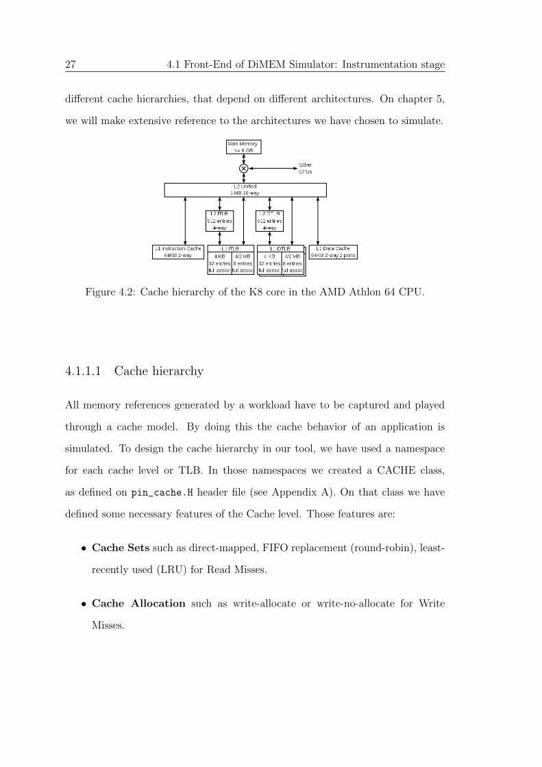
27 4.1 Front-End of DiMEM Simulator: Instrumentation stage
different cache hierarchies, that depend on different architectures. On chapter 5,
we will make extensive reference to the architectures we have chosen to simulate.
Figure 4.2: Cache hierarchy of the K8 core in the AMD Athlon 64 CPU.
4.1.1.1 Cache hierarchy
All memory references generated by a workload have to be captured and played
through a cache model. By doing this the cache behavior of an application is
simulated. To design the cache hierarchy in our tool, we have used a namespace
for each cache level or TLB. In those namespaces we created a CACHE class,
as defined on pin_cache.H header file (see Appendix A). On that class we have
defined some necessary features of the Cache level. Those features are:
• Cache Sets such as direct-mapped, FIFO replacement (round-robin), least-
recently used (LRU) for Read Misses.
• Cache Allocation such as write-allocate or write-no-allocate for Write
Misses.
4. IMPLEMENTATION OF DIMEM SIMULATOR 28
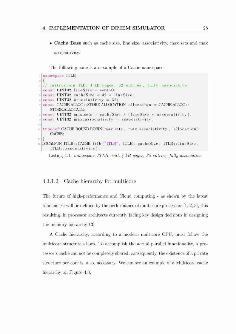
• Cache Base such as cache size, line size, associativity, max sets and max
associativity.
The following code is an example of a Cache namespace:
1 namespace ITLB2 {3 // i n s t r u c t i o n TLB: 4 kB pages , 32 en t r i e s , f u l l y a s s o c i a t i v e4 const UINT32 l i n e S i z e = 4∗KILO;5 const UINT32 cacheS i ze = 32 ∗ l i n e S i z e ;6 const UINT32 a s s o c i a t i v i t y = 32 ;7 const CACHEALLOC: : STORE ALLOCATION a l l o c a t i o n = CACHEALLOC: :
STOREALLOCATE;8 const UINT32 max sets = cacheS i ze / ( l i n e S i z e ∗ a s s o c i a t i v i t y ) ;9 const UINT32 max a s s o c i a t i v i t y = a s s o c i a t i v i t y ;
10
11 typede f CACHE ROUNDROBIN(max sets , max as soc i a t i v i t y , a l l o c a t i o n )CACHE;
12 }13 LOCALFUN ITLB : :CACHE i t l b ( ”ITLB” , ITLB : : cacheSize , ITLB : : l i n e S i z e ,
ITLB : : a s s o c i a t i v i t y ) ;
Listing 4.1: namespace ITLB, with 4 kB pages, 32 entries, fully associative
4.1.1.2 Cache hierarchy for multicore
The future of high-performance and Cloud computing - as shown by the latest
tendencies- will be defined by the performance of multi-core processors [1, 2, 3]; this
resulting, in processor architects currently facing key design decisions in designing
the memory hierarchy[13].
A Cache hierarchy, according to a modern multicore CPU, must follow the
multicore structure’s laws. To accomplish the actual parallel functionality, a pro-
cessor’s cache can not be completely shared, consequently, the existence of a private
structure per core is, also, necessary. We can see an example of a Multicore cache
hierarchy on Figure 4.3.

29 4.1 Front-End of DiMEM Simulator: Instrumentation stage
Carnegie Mellon
Now Let’s Consider Consistency Issues with the Caches
Todd Mowry & Dave Eckhardt 15-‐410: Intro to Parallelism 15
CPU 0 CPU 1 CPU 2 CPU N …
Memory
TLB 0 TLB 1 TLB 2 TLB N
L3 Cache
L2 $
L1 $
L2 $
L1 $
L2 $
L1 $
L2 $
L1 $
Figure 4.3: An example of a Multicore cache hierarchy
Allcache Pintool provides a single-core hierarchy example, as described above.
In order to extend its functionality, for more than one cores, we had to render the
Listing 4.1, as well as, all cache hierarchy namespaces, configurable. To accom-
plish that we had to insert a new Libraries package, in our code, the Boost C++
Libraries (boost.org). Those libraries are based on the standard libraries and they
are used to promote the flexibility and efficiency of code [6]. We chose to use the
local.hpp library, which has been made to enable us use MACROs in C++.
We need MACROs to make a configurable cache hierarchy for every core of the
system. To do that, we had to change the following code:
1 LOCALFUN ITLB : :CACHE i t l b ( ”ITLB” , ITLB : : cacheSize , ITLB : : l i n e S i z e ,ITLB : : a s s o c i a t i v i t y ) ;
Listing 4.2: ITLB::CACHE itlb() for single-core
to make use of BOOST Libraries, as below:
1 extern ITLB : :CACHE i t l b s [CORENUM] ;2
3 #de f i n e BOOST PP LOCAL LIMITS (0 , CORENUM − 1)4 #de f i n e BOOST PP LOCALMACRO(n) \5 ITLB : :CACHE( ”ITLB ” #n , ITLB : : cacheSize , ITLB : : l i n e S i z e , ITLB : :
a s s o c i a t i v i t y ) ,

4. IMPLEMENTATION OF DIMEM SIMULATOR 30
Figure 4.4: local.hpp File Reference
6
7 ITLB : :CACHE i t l b s [ ] =8 {9 #inc lude ” . . / . . / . . / boo s t 1 60 0 / boost / p r ep ro c e s s o r / i t e r a t i o n / d e t a i l /
l o c a l . hpp”10 } ;
Listing 4.3: ITLB::CACHE itlb() for multicore
We, finally, had to define the number of cores in our code, to make it fully
customizable. So we also added in our code the following line:
1 #de f i n e CORENUM 4
Listing 4.4: Define the number of cores
CORE_NUM not only is an argument that defines the number of Private Cache
levels (see lines 1 & 3 of Listing 4.3), but it also serves in many other points of our
pintool.
In general, the modern CPUs have, at least, one Unified/Shared Cache level
following the Private ones. That is not a commitment and it depends on each
architecture (e.g. ARM Cortex A-53 does not have any Unified Cache level).
31 4.1 Front-End of DiMEM Simulator: Instrumentation stage
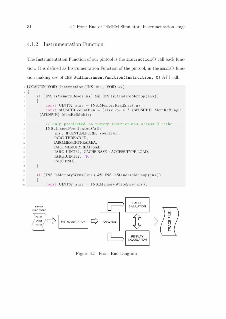
4.1.2 Instrumentation Function
The Instrumentation Function of our pintool is the Instruction() call back func-
tion. It is defined as Instrumentation Function of the pintool, in the main() func-
tion making use of INS_AddInstrumentFunction(Instruction, 0) API call.
1 LOCALFUN VOID In s t r u c t i o n ( INS ins , VOID ∗v )2 {3 i f ( INS IsMemoryRead ( i n s ) && INS IsStandardMemop ( i n s ) )4 {5 const UINT32 s i z e = INS MemoryReadSize ( i n s ) ;6 const AFUNPTR countFun = ( s i z e <= 4 ? (AFUNPTR) MemRefSingle
: (AFUNPTR) MemRefMulti ) ;7
8 // only pred icated−on memory i n s t r u c t i o n s a c c e s s D−cache9 INS Ins e r tPred i ca t edCa l l (
10 ins , IPOINT BEFORE, countFun ,11 IARG THREAD ID,12 IARGMEMORYREADEA,13 IARG MEMORYREAD SIZE,14 IARG UINT32 , CACHE BASE : :ACCESS TYPE LOAD,15 IARG UINT32 , ’R ’ ,16 IARG END) ;17 }18
19 i f ( INS IsMemoryWrite ( i n s ) && INS IsStandardMemop ( i n s ) )20 {21 const UINT32 s i z e = INS MemoryWriteSize ( i n s ) ;
Figure 4.5: Front-End Diagram
4. IMPLEMENTATION OF DIMEM SIMULATOR 32
22 const AFUNPTR countFun = ( s i z e <= 4 ? (AFUNPTR) MemRefSingle: (AFUNPTR) MemRefMulti ) ;
23
24 // only pred icated−on memory i n s t r u c t i o n s a c c e s s D−cache25 INS Ins e r tPred i ca t edCa l l (26 ins , IPOINT BEFORE, countFun ,27 IARG THREAD ID,28 IARGMEMORYWRITEEA,29 IARG MEMORYWRITE SIZE,30 IARG UINT32 , CACHE BASE : : ACCESS TYPE STORE,31 IARG UINT32 , ’W’ ,32 IARG END) ;33 }34
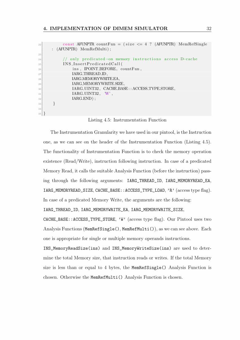
35 }Listing 4.5: Instrumentation Function
The Instrumentation Granularity we have used in our pintool, is the Instruction
one, as we can see on the header of the Instrumentation Function (Listing 4.5).
The functionality of Instrumentation Function is to check the memory operation
existence (Read/Write), instruction following instruction. In case of a predicated
Memory Read, it calls the suitable Analysis Function (before the instruction) pass-
ing through the following arguments: IARG_THREAD_ID, IARG_MEMORYREAD_EA,
IARG_MEMORYREAD_SIZE, CACHE_BASE::ACCESS_TYPE_LOAD, ’R’ (access type flag).
In case of a predicated Memory Write, the arguments are the following:
IARG_THREAD_ID, IARG_MEMORYWRITE_EA, IARG_MEMORYWRITE_SIZE,
CACHE_BASE::ACCESS_TYPE_STORE, ’W’ (access type flag). Our Pintool uses two
Analysis Functions (MemRefSingle(), MemRefMulti()), as we can see above. Each
one is appropriate for single or multiple memory operands instructions.
INS_MemoryReadSize(ins) and INS_MemoryWriteSize(ins) are used to deter-
mine the total Memory size, that instruction reads or writes. If the total Memory
size is less than or equal to 4 bytes, the MemRefSingle() Analysis Function is
chosen. Otherwise the MemRefMulti() Analysis Function is chosen.
33 4.1 Front-End of DiMEM Simulator: Instrumentation stage
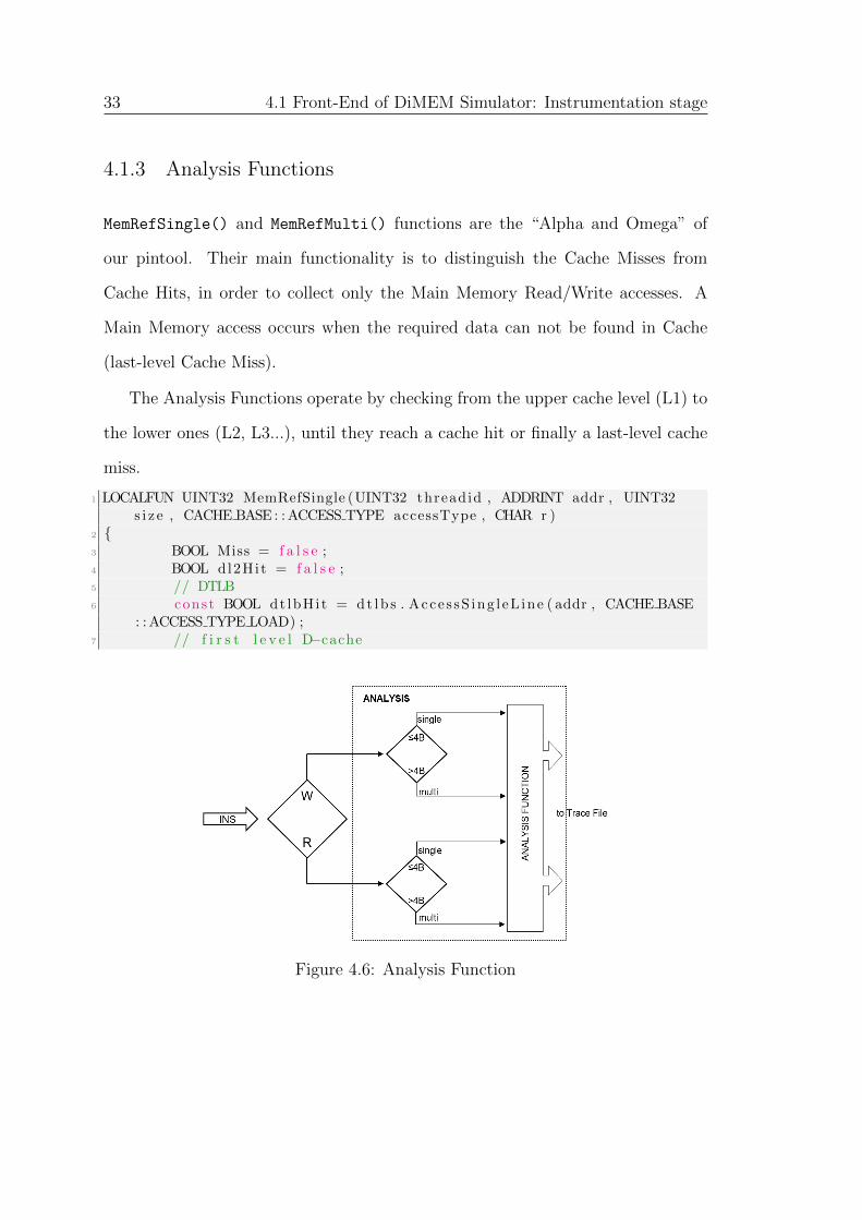
4.1.3 Analysis Functions
MemRefSingle() and MemRefMulti() functions are the “Alpha and Omega” of
our pintool. Their main functionality is to distinguish the Cache Misses from
Cache Hits, in order to collect only the Main Memory Read/Write accesses. A
Main Memory access occurs when the required data can not be found in Cache
(last-level Cache Miss).
The Analysis Functions operate by checking from the upper cache level (L1) to
the lower ones (L2, L3...), until they reach a cache hit or finally a last-level cache
miss.
1 LOCALFUN UINT32 MemRefSingle (UINT32 threadid , ADDRINT addr , UINT32s i z e , CACHE BASE : :ACCESS TYPE accessType , CHAR r )
2 {3 BOOL Miss = f a l s e ;4 BOOL dl2Hit = f a l s e ;5 // DTLB6 const BOOL dt lbHit = dt lb s . Acce s sS ing l eL ine ( addr , CACHE BASE
: :ACCESS TYPE LOAD) ;7 // f i r s t l e v e l D−cache
Figure 4.6: Analysis Function
4. IMPLEMENTATION OF DIMEM SIMULATOR 34
8 const BOOL dl1Hit = d l1 s . Acce s sS ing l eL ine ( addr , accessType ) ;9 // second l e v e l u n i f i e d Cache
10 i f ( ! d l1Hit )11 {12 dl2Hit = d l2 s . Access ( addr , s i z e , accessType ) ;13 i f ( ! d l2Hit )14 Miss = true ;15 }16 pena l ty = PenaltyCalc ( dt lbHit , dl1Hit , d l2Hit ) ;17 i f (Miss )18 {19 RecordAtTable ( threadid , addr , r , penalty , ’R ’ ) ;20 ram count++;21 }22 e l s e23 {24 RecordCachePenalty ( threadid , pena l ty ) ;25 }26 re turn 0 ;27 }
Listing 4.6: An Analysis Function without multithreading functionality
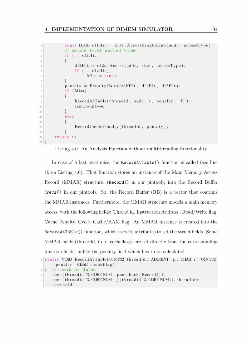
In case of a last level miss, the RecordAtTable() function is called (see line
19 on Listing 4.6). That function stores an instance of the Main Memory Access
Record (MMAR) structure, (Record() in our pintool), into the Record Buffer
(recs() in our pintool). So, the Record Buffer (RB) is a vector that contains
the MMAR instances. Furthermore, the MMAR structure models a main memory
access, with the following fields: Thread id, Instruction Address , Read/Write flag,
Cache Penalty, Cycle, Cache/RAM flag. An MMAR instance is created into the
RecordAtTable() function, which uses its attributes to set the struct fields. Some
MMAR fields (threadId, ip, r, cacheflags) are set directly from the corresponding
function fields, unlike the penalty field which has to be calculated.
1 s t a t i c VOID RecordAtTable (UINT32 threadid , ADDRINT ip , CHAR r , UINT32penalty , CHAR cacheFlag )
2 { // record at Buf f e r3 r e c s [ thread id % CORENUM] . push back ( Record ( ) ) ;4 r e c s [ thread id % CORENUM] [ j [ thread id % CORENUM] ] . thread id=
thread id ;

35 4.1 Front-End of DiMEM Simulator: Instrumentation stage
5 r e c s [ thread id % CORENUM] [ j [ thread id % CORENUM] ] . ip=ip ;6 r e c s [ thread id % CORENUM] [ j [ thread id % CORENUM] ] . r=r ;7 r e c s [ thread id % CORENUM] [ j [ thread id % CORENUM] ] . pena l ty=penalty
+ cachePena l t i e s [ thread id % coreNUM ] ;8 r e c s [ thread id % CORENUM] [ j [ thread id % CORENUM] ] . c y c l e =0;9 r e c s [ thread id % CORENUM] [ j [ thread id % CORENUM] ] . cacheFlag=
cacheFlag ;10 j [ thread id % CORENUM]++;11 cachePena l t i e s [ thread id % CORENUM] = 0 ;12 }
Listing 4.7: RecordAtTable() with multithreading functionality
Between two Main Memory Accesses (MMAR1, MMAR2) which are stored in the
RB, there have, actually, been much more -not stored- Cache Hits. These are
useless for the Simulation, but their additive cache penalty is equal to the Cycles
between MMAR1 and MMAR2. This functionality has been achieved by inserting the
RecordCachePenalty(threadid, penalty) in the Analysis Functions, to sum up
each Cache Penalty, between two Cache Misses.
1 s t a t i c VOID RecordCachePenalty (UINT32 threadid , UINT32 pena l ty )2 {3 //keep the add i t i v e pena l ty4 cachePena l t i e s [ thread id % CORENUM]= cachePena l t i e s [ thread id %
CORENUM] + penal ty ;5 }
Listing 4.8: RecordCachePenalty() with multithreading functionality
The Record Buffer’s Penalty is calculated by adding the additive cache penalty
to the current penalty (see line 9 on Listing 4.7). The current Penalty is calculated
by using the PenaltyCalc(dtlbHit, dl1Hit, dl2Hit) function.
1 LOCALFUN std : : s i z e t PenaltyCalc (BOOL boo l t l bH i t , BOOL boo l l 1H i t ,BOOL boo l l 2H i t )
2 {3 std : : s i z e t i n t t l bH i t = ( boo l t l bH i t ) ? 1 : 0 ;4 std : : s i z e t i n t l 1H i t = ( boo l l 1H i t ) ? 1 : 0 ;5 std : : s i z e t i n t l 2H i t = ( boo l l 2H i t ) ? 1 : 0 ;6 re turn ( i n t t l bH i t ∗TLB PENALTY) + ( i n t l 1H i t ∗L1 PENALTY) + (
i n t l 2H i t ∗L2 PENALTY) ;

4. IMPLEMENTATION OF DIMEM SIMULATOR 36
7 }
Listing 4.9: PenaltyCalc() function
PenaltyCalc() uses the following boolean attributes to calculate the Penalty of
an Instruction: dtlbHit, dl1Hit, dl2Hit, ... in combination with the defined
values of TLB_PENALTY, L1_PENALTY, L2_PENALTY, ... (see Listing 4.9).
1 #de f i n e TLB PENALTY 202 #de f i n e L1 PENALTY 33 #de f i n e L2 PENALTY 15
Listing 4.10: Cache Level Latencies and DTLB Miss Penalty #defines
4.1.4 Instrumentation Output
As described above, the back-end driver of our Simulator is DRAMSim2[28]. Trace-
driven simulation is a popular technique for conducting memory performance stud-
ies. In standalone mode, DRAMSim2 can simulate Memory-System traces. A
suitable trace file for DRAMSim2 has the following format:
1 0x7f64768732d0 P FETCH 12 0 x7f fd16a5a538 PMEMWR 83 0 x7f6476876a40 P FETCH 124 0 x7f6476a94e70 PMEMRD 615 0 x7f6476a95000 PMEMRD 79
Listing 4.11: A DRAMSim2 Trace File sample
The first column indicates the Instruction’s Virtual Address, the second one the
Instruction’s Type and the last column indicates the Cycle of each Instruction. To
communicate the front-end driver, with the analogous one back-end, it is necessary
for our pintool to generate the appropriate Trace Sequence.

37 4.1 Front-End of DiMEM Simulator: Instrumentation stage
4.1.4.1 Trace file
The functionality of writing into a Tracefile, has been added to our Simulator. To
achieve that, the following Command-line Switches have been added:
1 KNOB<s t r i ng> KnobOutputFile (KNOBMODEWRITEONCE, ” p in t oo l ” , ”o” ,”TraceFi l e . t r c ” , ” s p e c i f y t r a c e f i l e name” ) ;
2 KNOB<BOOL> KnobValues (KNOBMODEWRITEONCE, ” p in t oo l ” , ” va lue s ” , ”1” ,”Output memory va lue s reads and wr i t t en ” ) ;
as well as, the following lines in the main() function:
1 TraceFi l e . open (KnobOutputFile . Value ( ) . c s t r ( ) ) ;2 TraceFi l e . s e t f ( i o s : : showbase ) ;
Now, we had to load the Tracefile.trc like the three-column DRAMSim2
Tracefile format:
1 f o r ( i =0; i<r e c . s i z e ( ) ; i++)2 {3 i f ( r e c [ i ] . cacheFlag==’R ’ )4 {5 i f ( r e c [ i ] . r==’F ’ )6 {7 TraceFi l e << hex << r e c [ i ] . ip << ” ” << ”P FETCH” << ” ” << dec
<< r e c [ i ] . pena l ty ;8 TraceFi l e << endl ;9 }
10 e l s e i f ( r e c [ i ] . r==’W’ )11 {12 TraceFi l e << hex << r e c [ i ] . ip << ” ” << ”PMEMWR” << ” ”
<< dec << r e c [ i ] . pena l ty ;13 TraceFi l e << endl ;14 }15 e l s e16 {17 TraceFi l e << hex << r e c [ i ] . ip << ” ” << ”PMEMRD” << ” ”
<< dec << r e c [ i ] . pena l ty ;18 TraceFi l e << endl ;19 }20 }21 }
Listing 4.12: Trace File generation code

4. IMPLEMENTATION OF DIMEM SIMULATOR 38
4.1.4.2 Record Buffer
In the shared-library mode, DRAMSim2 exposes the basic functionality by creating
a new object (MemorySystem) and by adding requests to that. There is no need
for an external Tracefile, in the shared-library mode. The role of the Tracefile has
been played by the Record Buffer (RB), as described above. In fact, RB is the
source of the Tracefile.
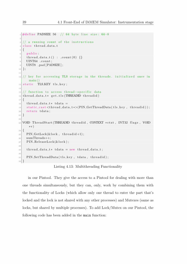
4.1.5 Multithreading Functionality
Pin supports the instrumentation of multi-threaded applications, along with the
single-threaded ones. The operating system controls the scheduling of different
threads of the application. Pin charges each thread with a unique ID different
from the native process ID assigned by the operating system. It does so in order
to distinguish between the different threads of the application. Pin assigns the 1st
thread (i.e. the main thread) with thread ID 0 and each additional new thread the
next sequential ID (i.e. 1, 2, 3) and so on. This way, when a five-threaded workload
is used to conduct a study, PIN distinguishes between threads by assigning each
thread a different ID, starting from ID 0 (for the main thread) and continuing with
the remaining four threads.
The philosophy of multithreading in our Pintool is that every system core deals
with more than one threads simultaneously. The multi-threading functionality has
been achieved by making the following changes on our pintool. First of all, we had
to change the Cache hierarchy code, as described on subsection 4.1.1.2 above. The
next step was to add the thread_data_t class and the ThreadStart() function,
39 4.1 Front-End of DiMEM Simulator: Instrumentation stage
1 #de f i n e PADSIZE 56 // 64 byte l i n e s i z e : 64−82
3 // a running count o f the i n s t r u c t i o n s4 c l a s s th r ead da ta t5 {6 pub l i c :7 th r ead da ta t ( ) : count (0 ) {}8 UINT64 count ;9 UINT8 pad [PADSIZE ] ;
10 } ;11
12 // key f o r a c c e s s i n g TLS s to rage in the threads . i n i t i a l i z e d once inmain ( )
13 s t a t i c TLS KEY t l s k e y ;14
15 // func t i on to ac c e s s thread−s p e c i f i c data16 th r ead da ta t ∗ g e t t l s (THREADID thread id )17 {18 th r ead da ta t ∗ tdata =19 s t a t i c c a s t <th r ead da ta t ∗>(PIN GetThreadData ( t l s k ey , thread id ) ) ;20 re turn tdata ;21 }22
23 VOID ThreadStart (THREADID threadid , CONTEXT ∗ ctxt , INT32 f l a g s , VOID∗v )
24 {25 PIN GetLock(&lock , thread id+1) ;26 numThreads++;27 PIN ReleaseLock(& lock ) ;28
29 th r ead da ta t ∗ tdata = new thr ead da ta t ;30
31 PIN SetThreadData ( t l s k ey , tdata , thread id ) ;32 }
Listing 4.13: Multithreading Functionality
in our Pintool. They give the access to a Pintool for dealing with more than
one threads simultaneously, but they can, only, work by combining them with
the functionality of Locks (which allow only one thread to enter the part that’s
locked and the lock is not shared with any other processes) and Mutexes (same as
locks, but shared by multiple processes). To add Lock/Mutex on our Pintool, the
following code has been added in the main function:

4. IMPLEMENTATION OF DIMEM SIMULATOR 40
1 // I n i t i a l i z e the lock2 PIN InitLock(& lock ) ;3
4 // I n i t i a l i z e the mutexes5 PIN MutexInit(&Mutex) ;6
7 // Obtain a key f o r TLS s to rage .8 t l s k e y = PIN CreateThreadDataKey (0) ;9
10 // Reg i s t e r ThreadStart to be c a l l e d when a thread s t a r t s .11 PIN AddThreadStartFunction ( ThreadStart , 0) ;
Listing 4.14: Initialize the lock/mutex
as well, the following in the Fini function:
1 PIN MutexFini(&Mutex) ;
Every time, now, the Pintool is dealing with a threadId, it is enclosed between
a Lock or a Mutex. For example:
1 s t a t i c VOID RecordAtTable (UINT32 threadid , ADDRINT ip , CHAR r , UINT32penalty , CHAR cacheFlag )
2 { // record at Buf f e r3 PIN MutexLock(&Mutex) ;4 r e c s [ thread id % CORENUM] . push back ( Record ( ) ) ;5 r e c s [ thread id % CORENUM] [ j [ thread id % CORENUM] ] . thread id=thread id ;6 r e c s [ thread id % CORENUM] [ j [ thread id % CORENUM] ] . ip=ip ;7 r e c s [ thread id % CORENUM] [ j [ thread id % CORENUM] ] . r=r ;8 r e c s [ thread id % CORENUM] [ j [ thread id % CORENUM] ] . pena l ty=penalty +
cachePena l t i e s [ thread id % coreNUM ] ;9 r e c s [ thread id % CORENUM] [ j [ thread id % CORENUM] ] . c y c l e =0;
10 r e c s [ thread id % CORENUM] [ j [ thread id % CORENUM] ] . cacheFlag=cacheFlag;
11 j [ thread id % CORENUM]++;12 cachePena l t i e s [ thread id % CORENUM] = 0 ;13 PIN MutexUnlock(&Mutex) ;14 }
Listing 4.15: Mutex example
Listing 4.15 indicates the last (but not least) change of the multithreading
functionality, we have rendered. Every one-dimensional table and vector had to
be replaced by a multi-dimensional one, to “simulate” the multicore design.
I.e. the recs.push_back(Record()) has been replaced by recs[threadid %
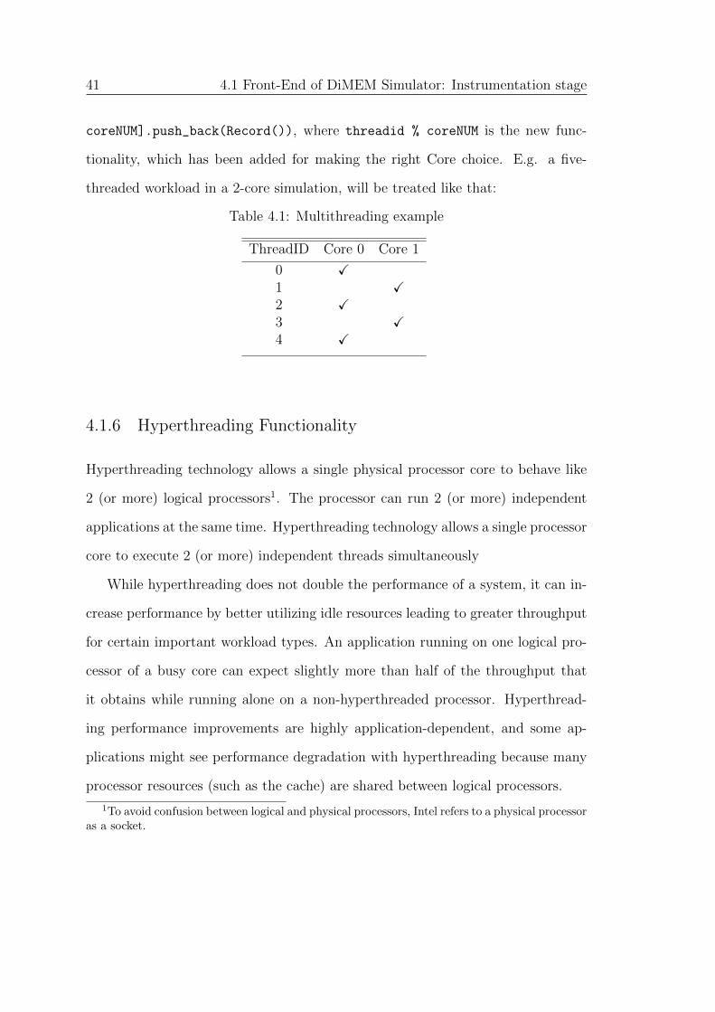
41 4.1 Front-End of DiMEM Simulator: Instrumentation stage
coreNUM].push_back(Record()), where threadid % coreNUM is the new func-
tionality, which has been added for making the right Core choice. E.g. a five-
threaded workload in a 2-core simulation, will be treated like that:
Table 4.1: Multithreading example
ThreadID Core 0 Core 1
0 X1 X2 X3 X4 X
4.1.6 Hyperthreading Functionality
Hyperthreading technology allows a single physical processor core to behave like
2 (or more) logical processors1. The processor can run 2 (or more) independent
applications at the same time. Hyperthreading technology allows a single processor
core to execute 2 (or more) independent threads simultaneously
While hyperthreading does not double the performance of a system, it can in-
crease performance by better utilizing idle resources leading to greater throughput
for certain important workload types. An application running on one logical pro-
cessor of a busy core can expect slightly more than half of the throughput that
it obtains while running alone on a non-hyperthreaded processor. Hyperthread-
ing performance improvements are highly application-dependent, and some ap-
plications might see performance degradation with hyperthreading because many
processor resources (such as the cache) are shared between logical processors.
1To avoid confusion between logical and physical processors, Intel refers to a physical processoras a socket.
4. IMPLEMENTATION OF DIMEM SIMULATOR 42
As is clear from the above, the Hyperthreading Functionality is essential to a
modern processor. To add that functionality in our Pintool, the following addi-
tions, have been made:
1 #de f i n e HYPERTHREADING 2 // THREADS PER CORE, 1 = NO HYPERTHREADING2
3 coreNUM = CORENUM∗HYPERTHREADING;
as well as, the CORE_NUM has been replaced by coreNUM, everywhere except in
the Cache Hierarchy part, in order to maintain the logical processors, as they were.
4.2 Back-End of DiMEM Simulator: Simulation stage
The Simulation Stage of the DiMEM Simulator was designed by Orion Papadakis[26].
His Diploma Thesis focuses on the Pintool’s Simulation Preparation functionality,
both from theoretical and implementation point of view, so that the Pintool ob-
tains more complete system and useful tool characteristics than a simple Memory
Tracing Pintool. The implemented features which have been added on the pintool
are the following:
1. Reordering, Approximate Timing and Sorting of the Multithreaded Trace
2. Making use of the capabilities of DRAMSim2 Cycle Accurate Memory Sys-
tem Simulator,
3. Implementation of Disaggregate Memory Behaviour
4. Speeding-up the Simulation with “Skip Mode”.
CHAPTER5Evaluation and Experimental Results
5.1 Evaluation
The section of Evaluation is about the CPU, DRAM and Benchmark choices. The
first are presented by CPU Metrics and the DRAM model are described in the
DRAM Metrics. After that, a Cloudsuite benchmark suites summary performed.
5.1.1 CPU Metrics
As it has already been explained, the DiMEM Simulator is ISA portable. That
feature gives the user the valuable freedom of selection, to decide which CPU
Model he wants to use coupled with a Memory System. The user can modify the
Cache Size, Associativity, Penalties, the number of Cores, to enable/disable the
Hyperthreading etc.
Three popular CPUs for Cloud Servers, are used in the current thesis:
1. ARM Cortex-A53
2. ARM Cortex-A57
3. IBM Power8
5. EVALUATION AND EXPERIMENTAL RESULTS 44
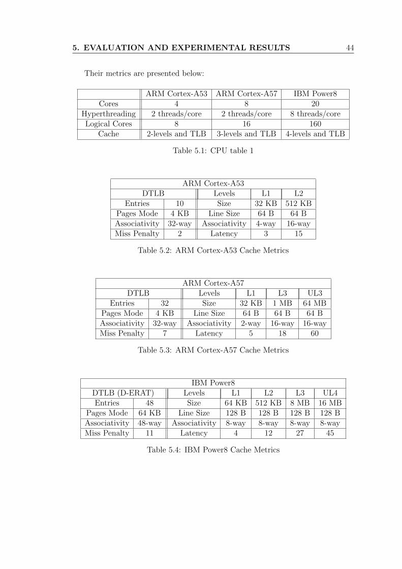
Their metrics are presented below:
ARM Cortex-A53 ARM Cortex-A57 IBM Power8Cores 4 8 20
Hyperthreading 2 threads/core 2 threads/core 8 threads/coreLogical Cores 8 16 160
Cache 2-levels and TLB 3-levels and TLB 4-levels and TLB
Table 5.1: CPU table 1
ARM Cortex-A53DTLB Levels L1 L2
Entries 10 Size 32 KB 512 KBPages Mode 4 KB Line Size 64 B 64 BAssociativity 32-way Associativity 4-way 16-wayMiss Penalty 2 Latency 3 15
Table 5.2: ARM Cortex-A53 Cache Metrics
ARM Cortex-A57DTLB Levels L1 L3 UL3
Entries 32 Size 32 KB 1 MB 64 MBPages Mode 4 KB Line Size 64 B 64 B 64 BAssociativity 32-way Associativity 2-way 16-way 16-wayMiss Penalty 7 Latency 5 18 60
Table 5.3: ARM Cortex-A57 Cache Metrics
IBM Power8DTLB (D-ERAT) Levels L1 L2 L3 UL4Entries 48 Size 64 KB 512 KB 8 MB 16 MB
Pages Mode 64 KB Line Size 128 B 128 B 128 B 128 BAssociativity 48-way Associativity 8-way 8-way 8-way 8-wayMiss Penalty 11 Latency 4 12 27 45
Table 5.4: IBM Power8 Cache Metrics
45 5.1 Evaluation
5.1.2 DRAM Metrics
The Memory System is portable, as well as, the CPU. The user can modify and ex-
periment with his/her own choices. The Device Ini and System Ini of DRAMSim2
contain many variables which can be modified. A modified Micron MT40A1G4HX-
083E DDR4 SDRAM[Micron site] it is used in the current thesis.
The original model has by default 4 GB of total storage, but the benchmarks
that the current thesis used had an average less than 1 GB footprint. So, the Rows
and Columns were modified, in order to shrink the original model to 1 GB of total
storage.
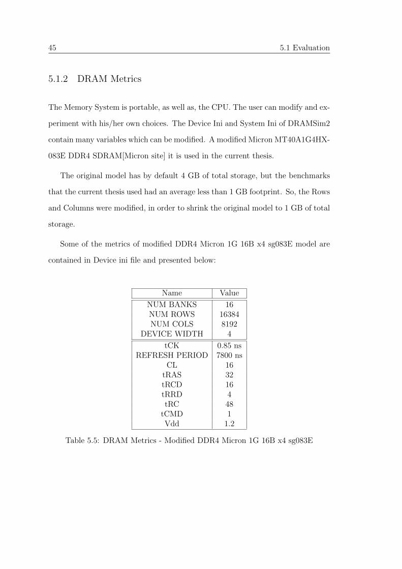
Some of the metrics of modified DDR4 Micron 1G 16B x4 sg083E model are
contained in Device ini file and presented below:
Name Value
NUM BANKS 16NUM ROWS 16384NUM COLS 8192
DEVICE WIDTH 4
tCK 0.85 nsREFRESH PERIOD 7800 ns
CL 16tRAS 32tRCD 16tRRD 4tRC 48
tCMD 1Vdd 1.2
Table 5.5: DRAM Metrics - Modified DDR4 Micron 1G 16B x4 sg083E

5. EVALUATION AND EXPERIMENTAL RESULTS 46
5.1.3 Cloud Benchmarks
Cloud benchmarks are certain tests which are applied to cloud computing services
offered by companies and organizations. More broadly speaking, we would say
that benchmarks are not merely tests, but they are considered best practices for
certain components of the Cloud computing which are examined. Benchmarking
is used for performance analysis and, from every aspect and type of computing,
one can discover that there are many benchmarking tests (pieces of software)
available, proprietary or not, in order to be utilized by the tester. For example,
let us refer to the geekbench product, which is a commercial CPU benchmarking
solution. Geekbench has got 27 different workloads (tests) at its disposal: namely,
13 integer tests, 10 floating-point tests and, lastly, 4 memory tests[1]. There are
many cloud benchmarks of the kind, such as those developed by large market-share
holders such as Google (PerfKitBenchmarker) and Oracle, and other companies
such as Upcloud. The one used in this thesis is CloudSuite[10, 25].
5.1.3.1 Cloudsuite
The CloudSuite employs certain specific criteria in order to evaluate the perfor-
mance and efficiency of the cloud services to be assessed. The scale-out services
(as opposed to the traditional ones) examined by the Suite are the most popular
ones [10] and are the following:
a) Data serving
b) Media streaming
47 5.1 Evaluation
c) Web search
Furthermore, some additional ones, as included in CloudSuite 3.0, are:
g) Data analytics
h) Graph analytics
i) In-Memory analytics
j) Data caching
The examination of the aforementioned can depict the architectural behavior of
the system, database and data transport performance, storage velocity, media files
transmission, fault tolerance, web services throughput and performance scalability.
All the benchmarking tests should be performed when the system has reached a
steady state[10, 25].
Lastly, let us refer to two elements which have especially been utilized during
the course of this thesis. These are Data caching and Media streaming.
Data Caching
Data Caching is an online benchmark; it is meant to constritute a performance
criterion of how well the system does when it is presented with an arbitrary amount
of online requests. The manner in which it functions emulates Twitter users and
memcached software is used to this end. The performance metrics put to use are
the number of requests served per second and the latency percent for the total of
these requests. The idea here is that, since data access is slow, and every failure to
5. EVALUATION AND EXPERIMENTAL RESULTS 48
reach to cache and retrieve a piece of data will result in a disk request, the metrics
are thought to effectively measure the performance of data caching, which results
in quick data access.
Media Streaming
Media Streaming benchmark, on the other hand, is still an online benchmark, but
referring to multimedia access performance. An HTTP Connection is made at first
and, then, a flexible total of video-streaming requests is sent to the servers. Videos
of all types and quality can be accessed and the performance metrics calculated
are the streaming bandwidth and the average delay for the reply to each request
that was sent.
5.2 Experimental Process
In that section the experimental process strategy is going to be described. The re-
sult reliability achievement is the main problem of an experimental process design.
We developed on the Simulator the functionality of the Skip mode, because of the
time consuming simulation as a result of the large overhead over the benchmark
execution time[31]. Skip mode, in essence, is a sampling method, consequently,
the existence of the statistical error ε cannot be hidden; it has to be determined,
as well as the sampling rate, to make the reader able to evaluate the result’s relia-
bility. The sampling rate, as a function of ”how many samples”, describes ”when”,
a measurement, or in our case a piece of simulation, must be applied for the result
reliability maintenance.

49 5.2 Experimental Process
We choose to use a simulation sample size of 2 Billion benchmark instructions,
our experiments The trade-off simulation sample size vs simulation time had lead
us to that choice. The sample has to be large enough to let the benchmark unfold
its true workload execution, but always in the context of paying the least useful
overhead. So that, the 2 Billion was estimated as a good trade-off, because that
size is quite over the usual benchmark execution and simulation threshold, which is
1 Billion (eg the Ramulator [18] evaluation uses 10M main memory accesses which
approximately corresponds to 1% miss rate per Billion Instructions), and also the
overhead was not excessively high. The overhead affection was experimentally
observed.
The simulation result of the 2 Billion sampling must be scaled up to the whole
benchmark size, in order to produce the final result. At this point, the final result
must be accompanied with the corresponding ε.
To calculate the ε, a complete simulation, without sampling, is the one way.
But as a result of the time limitations, imposed by the complete simulation, (ex-
pected duration of Media Streaming∼ 90 days = 3 months or non-stop data flow
on Datacache), the solution of just a 4 times denser simulation has been chosen.
A simulation with higher density will not provide us with an accurate ε, but with
just an indication of our sample selection accuracy level.
Sample Selection: The samples must be uniformly distributed along the whole
benchmark instructions, to make the sampling representative. A simple Workload
Profiling Pintool was developed to instrument the benchmark and produce a last
level cache miss profile representation. The functionality of that Pintool is quite
simple. The whole benchmark is simply instrumented, in order to profile the last
level cache miss number of each window. That number is recorded to a .csv file,

5. EVALUATION AND EXPERIMENTAL RESULTS 50
so that profile can be depicted in a chart.
The offered knowledge of a last level cache miss profile chart give us the ability
to design the simulation process, in order to distribute in a uniform and statistically
correct way our simulation samples.
In order to achieve the corresponding and appropriate sampling distribution,
each benchmark has to be utilized separately.
Finally we have to say, that we have failed to take the Simulation results of the
Media Streaming Benchmark because after the final video streaming the Client
terminates and the Server restarts,making the problem of deleting the log files, as
a new Server container starts, after deleting the old one automatically.
Only the DataCaching Profiling and Utilization with 4GB memory size is pre-
sented bellow, as all the other profiles are the same.
5.2.1 Data Caching Profiling and Utilization
As we can see in figure 5.1, the diagram cannot be divided in any areas. We
observe that the majority of the values is 0,4 MPKI, except of the initialization
phase ones (the first 4 windows)
Due to that stability it was prefered to simulate a solid area. In that benchmark
we use 200 Million Instructions sized Windows, subsequently, to perform a 2 Billion
Instructions Simulation, we need 10 Windows (samples).
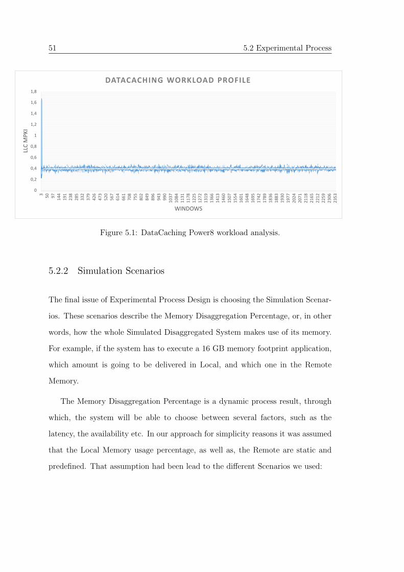
51 5.2 Experimental Process
0
0,2
0,4
0,6
0,8
1
1,2
1,4
1,6
1,8
35
09
71
44
19
12
38
28
53
32
37
94
26
47
35
20
56
76
14
66
17
08
75
58
02
84
98
96
94
39
90
10
37
10
84
11
31
11
78
12
25
12
72
13
19
13
66
14
13
14
60
15
07
15
54
16
01
16
48
16
95
17
42
17
89
18
36
18
83
19
30
19
77
20
24
20
71
21
18
21
65
22
12
22
59
23
06
23
53
LLC
MP
KI
WINDOWS
DATACACHING WORKLOAD PROFILE
Figure 5.1: DataCaching Power8 workload analysis.
5.2.2 Simulation Scenarios
The final issue of Experimental Process Design is choosing the Simulation Scenar-
ios. These scenarios describe the Memory Disaggregation Percentage, or, in other
words, how the whole Simulated Disaggregated System makes use of its memory.
For example, if the system has to execute a 16 GB memory footprint application,
which amount is going to be delivered in Local, and which one in the Remote
Memory.
The Memory Disaggregation Percentage is a dynamic process result, through
which, the system will be able to choose between several factors, such as the
latency, the availability etc. In our approach for simplicity reasons it was assumed
that the Local Memory usage percentage, as well as, the Remote are static and
predefined. That assumption had been lead to the different Scenarios we used:
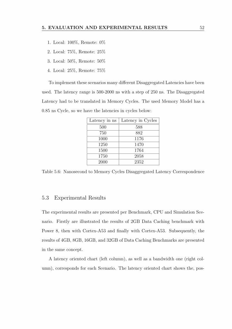
5. EVALUATION AND EXPERIMENTAL RESULTS 52
1. Local: 100%, Remote: 0%
2. Local: 75%, Remote: 25%
3. Local: 50%, Remote: 50%
4. Local: 25%, Remote: 75%
To implement these scenarios many different Disaggregated Latencies have been
used. The latency range is 500-2000 ns with a step of 250 ns. The Disaggregated
Latency had to be translated in Memory Cycles. The used Memory Model has a
0.85 ns Cycle, so we have the latencies in cycles below:
Latency in ns Latency in Cycles
500 588750 8821000 11761250 14701500 17641750 20582000 2352
Table 5.6: Nanosecond to Memory Cycles Disaggregated Latency Correspondence
5.3 Experimental Results
The experimental results are presented per Benchmark, CPU and Simulation Sce-
nario. Firstly are illustrated the results of 2GB Data Caching benchmark with
Power 8, then with Cortex-A53 and finally with Cortex-A53. Subsequently, the
results of 4GB, 8GB, 16GB, and 32GB of Data Caching Benchmarks are presented
in the same concept.
A latency oriented chart (left column), as well as a bandwidth one (right col-
umn), corresponds for each Scenario. The latency oriented chart shows the, pos-
53 5.3 Experimental Results
itive or negative, Overhead in total execution time over the 100-0 Scenario in a
stack bar per Disaggregation Latency Step. As total execution time, is defined the
addition between the Local and Disaggregated execution time.
With that kind of chart, we are able to observe how the Disaggregated nature
and behavior differs the benchmark execution time compared with the non Dis-
aggregated (scenario 100-0). The point that can be observed is that, the charts
depict the expected increase on the execution time. As the Disaggregated Latency
increases, so does the Overhead. That fact is the expected Disaggregated effect
over the total execution time.
The second kind of chart is about the Bandwidth. In that line chart the Average
Memory Bandwidth results in absolute values are depicted, also per Disaggregation
Latency Step. Here we can observe that as the Disaggregated Latency increases,
the Bandwidth falls. That phenomenon also validates the right Disaggregated
behavior of the DiMEM Simulator because the Disaggregated Latency enlarges
the time distance between the Memory Accesses and as a result we can observe
the Bandwidth loss.
5.3.1 Dense Data Caching Experimental Results
As noticed earlier, a denser experiment for Data Caching has been performed,
in order to evaluate that Benchmark’s experimental process. The Data Caching
Benchmark profile shows a stability on 0,4 MPKI.
The Dense Experiment results show 0.078% divergence in comparison with the
2 Billion Instructions Experiment. The above results were expected due to the
specific behavior of the workload profile.
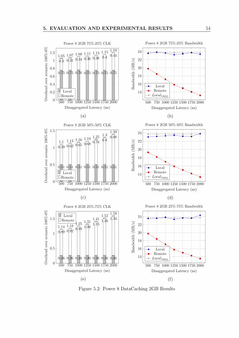
5. EVALUATION AND EXPERIMENTAL RESULTS 54
500 750 1000 1250 1500 1750 20000
0.2
0.4
0.6
0.8
1
1.21.05 1.07 1.09 1.11 1.13 1.15 1.19
0.3 0.31 0.34 0.36 0.38 0.4 0.44
0.75 0.75 0.76 0.75 0.75 0.75 0.75
Disaggregated Latency (ns)
Ove
rhea
dov
ersc
enar
io10
0%-0
%Power 8 2GB 75%-25% CLK
LocalRemote
(a)
500 750 1000 1250 1500 1750 2000
14
16
18
20
22
24
Disaggregated Latency (ns)
Ban
dw
idth
(MB
/s)
Power 8 2GB 75%-25% Bandwidth
LocalRemoteLocal100%
(b)
500 750 1000 1250 1500 1750 20000
0.5
1
1.5
1.1 1.13 1.16 1.19 1.25 1.31.39
0.59 0.62 0.65 0.68 0.74 0.80.88
0.51 0.51 0.51 0.51 0.51 0.51 0.51
Disaggregated Latency (ns)
Ove
rhea
dov
ersc
enar
io10
0%-0
%
Power 8 2GB 50%-50% CLK
LocalRemote
(c)
500 750 1000 1250 1500 1750 2000
14
16
18
20
22
24
Disaggregated Latency (ns)
Ban
dw
idth
(MB
/s)
Power 8 2GB 50%-50% Bandwidth
LocalRemoteLocal100%
(d)
500 750 1000 1250 1500 1750 20000
0.5
1
1.5
1.14 1.181.25
1.311.41
1.521.59
0.89 0.920.99
1.061.15
1.261.34
0.26 0.26 0.26 0.26 0.26 0.26 0.26
Disaggregated Latency (ns)
Ove
rhea
dov
ersc
enar
io10
0%-0
%
Power 8 2GB 25%-75% CLK
LocalRemote
(e)
500 750 1000 1250 1500 1750 2000
14
16
18
20
22
24
Disaggregated Latency (ns)
Ban
dw
idth
(MB
/s)
Power 8 2GB 25%-75% Bandwidth
LocalRemoteLocal100%
(f)
Figure 5.2: Power 8 DataCaching 2GB Results
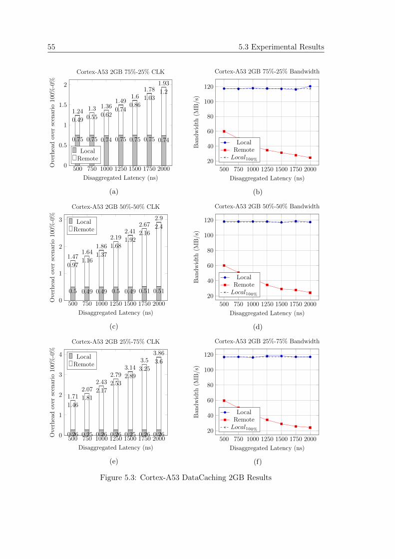
55 5.3 Experimental Results
500 750 1000 1250 1500 1750 20000
0.5
1
1.5
2
1.24 1.3 1.361.49
1.61.78
1.93
0.49 0.55 0.620.74
0.861.03
1.2
0.75 0.75 0.74 0.75 0.75 0.75 0.74
Disaggregated Latency (ns)
Ove
rhea
dov
ersc
enar
io10
0%-0
%
Cortex-A53 2GB 75%-25% CLK
LocalRemote
(a)
500 750 1000 1250 1500 1750 2000
20
40
60
80
100
120
Disaggregated Latency (ns)
Ban
dw
idth
(MB
/s)
Cortex-A53 2GB 75%-25% Bandwidth
LocalRemoteLocal100%
(b)
500 750 1000 1250 1500 1750 20000
1
2
3
1.471.64
1.86
2.192.41
2.672.9
0.971.16
1.37
1.681.92
2.162.4
0.5 0.49 0.49 0.5 0.49 0.51 0.51
Disaggregated Latency (ns)
Ove
rhea
dov
ersc
enar
io10
0%-0
%
Cortex-A53 2GB 50%-50% CLK
LocalRemote
(c)
500 750 1000 1250 1500 1750 2000
20
40
60
80
100
120
Disaggregated Latency (ns)
Ban
dw
idth
(MB
/s)
Cortex-A53 2GB 50%-50% Bandwidth
LocalRemoteLocal100%
(d)
500 750 1000 1250 1500 1750 20000
1
2
3
4
1.712.07
2.432.79
3.143.5
3.86
1.461.81
2.172.53
2.893.25
3.6
0.26 0.25 0.26 0.26 0.25 0.26 0.26
Disaggregated Latency (ns)
Ove
rhea
dov
ersc
enar
io10
0%-0
%
Cortex-A53 2GB 25%-75% CLK
LocalRemote
(e)
500 750 1000 1250 1500 1750 2000
20
40
60
80
100
120
Disaggregated Latency (ns)
Ban
dw
idth
(MB
/s)
Cortex-A53 2GB 25%-75% Bandwidth
LocalRemoteLocal100%
(f)
Figure 5.3: Cortex-A53 DataCaching 2GB Results

5. EVALUATION AND EXPERIMENTAL RESULTS 56
500 750 1000 1250 1500 1750 20000
0.5
1
1.5
2
1.251.38
1.51.63
1.761.88
2
0.50.63
0.760.88
1.011.13
1.25
0.75 0.75 0.75 0.74 0.75 0.75 0.75
Disaggregated Latency (ns)
Ove
rhea
dov
ersc
enar
io10
0%-0
%Cortex-A57 2GB 75%-25% CLK
LocalRemote
(a)
500 750 1000 1250 1500 1750 2000
20
40
60
80
100
120
Disaggregated Latency (ns)
Ban
dw
idth
(MB
/s)
Cortex-A57 2GB 75%-25% Bandwidth
LocalRemoteLocal100%
(b)
500 750 1000 1250 1500 1750 20000
1
2
3
1.491.75
22.25
2.52.75
3
0.991.24
1.491.75
1.992.24
2.49
0.5 0.5 0.5 0.51 0.5 0.5 0.51
Disaggregated Latency (ns)
Ove
rhea
dov
ersc
enar
io10
0%-0
%
Cortex-A57 2GB 50%-50% CLK
LocalRemote
(c)
500 750 1000 1250 1500 1750 2000
20
40
60
80
100
120
Disaggregated Latency (ns)
Ban
dw
idth
(MB
/s)
Cortex-A57 2GB 50%-50% Bandwidth
LocalRemoteLocal100%
(d)
500 750 1000 1250 1500 1750 20000
1
2
3
4
1.752.04
2.42
2.93.28
3.77
4.35
1.51.78
2.16
2.643.03
3.51
4.09
0.26 0.26 0.26 0.26 0.26 0.26 0.26
Disaggregated Latency (ns)
Ove
rhea
dov
ersc
enar
io10
0%-0
%
Cortex-A57 2GB 25%-75% CLK
LocalRemote
(e)
500 750 1000 1250 1500 1750 2000
20
40
60
80
100
120
Disaggregated Latency (ns)
Ban
dw
idth
(MB
/s)
Cortex-A57 2GB 25%-75% Bandwidth
LocalRemoteLocal100%
(f)
Figure 5.4: Cortex-A57 DataCaching 2GB Results

57 5.3 Experimental Results
500 750 1000 1250 1500 1750 20000
0.2
0.4
0.6
0.8
1
1.21.04 1.07 1.09 1.12 1.13 1.16 1.19
0.29 0.32 0.34 0.37 0.39 0.41 0.43
0.75 0.75 0.75 0.76 0.75 0.75 0.75
Disaggregated Latency (ns)
Ove
rhea
dov
ersc
enar
io10
0%-0
%
Power 8 4GB 75%-25% CLK
LocalRemote
(a)
500 750 1000 1250 1500 1750 200012
14
16
18
20
22
24
Disaggregated Latency (ns)
Ban
dw
idth
(MB
/s)
Power 8 4GB 75%-25% Bandwidth
LocalRemoteLocal100%
(b)
500 750 1000 1250 1500 1750 20000
0.5
1
1.5
1.09 1.14 1.19 1.24 1.291.34 1.37
0.59 0.64 0.69 0.73 0.780.84 0.87
0.5 0.5 0.51 0.51 0.51 0.5 0.5
Disaggregated Latency (ns)
Ove
rhea
dov
ersc
enar
io10
0%-0
%
Power 8 4GB 50%-50% CLK
LocalRemote
(c)
500 750 1000 1250 1500 1750 2000
14
16
18
20
22
24
Disaggregated Latency (ns)
Ban
dw
idth
(MB
/s)
Power 8 4GB 50%-50% Bandwidth
LocalRemoteLocal100%
(d)
500 750 1000 1250 1500 1750 20000
0.5
1
1.5
1.141.21 1.27
1.351.41
1.481.56
0.880.95 1.02
1.091.15
1.221.31
0.26 0.26 0.26 0.26 0.26 0.26 0.26
Disaggregated Latency (ns)
Ove
rhea
dov
ersc
enar
io10
0%-0
%
Power 8 4GB 25%-75% CLK
LocalRemote
(e)
500 750 1000 1250 1500 1750 2000
14
16
18
20
22
24
Disaggregated Latency (ns)
Ban
dw
idth
(MB
/s)
Power 8 4GB 25%-75% Bandwidth
LocalRemoteLocal100%
(f)
Figure 5.5: Power 8 DataCaching 4GB Results
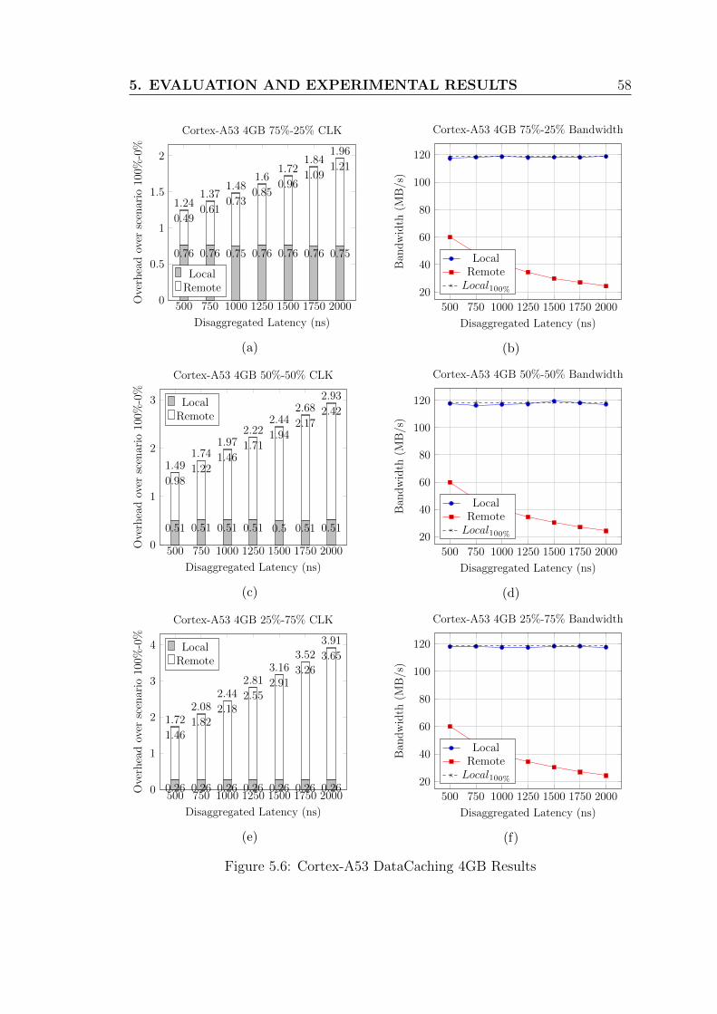
5. EVALUATION AND EXPERIMENTAL RESULTS 58
500 750 1000 1250 1500 1750 20000
0.5
1
1.5
2
1.241.37
1.481.6
1.721.84
1.96
0.490.61
0.730.85
0.961.09
1.21
0.76 0.76 0.75 0.76 0.76 0.76 0.75
Disaggregated Latency (ns)
Ove
rhea
dov
ersc
enar
io10
0%-0
%Cortex-A53 4GB 75%-25% CLK
LocalRemote
(a)
500 750 1000 1250 1500 1750 2000
20
40
60
80
100
120
Disaggregated Latency (ns)
Ban
dw
idth
(MB
/s)
Cortex-A53 4GB 75%-25% Bandwidth
LocalRemoteLocal100%
(b)
500 750 1000 1250 1500 1750 20000
1
2
3
1.491.74
1.972.22
2.442.68
2.93
0.981.22
1.461.71
1.942.17
2.42
0.51 0.51 0.51 0.51 0.5 0.51 0.51
Disaggregated Latency (ns)
Ove
rhea
dov
ersc
enar
io10
0%-0
%
Cortex-A53 4GB 50%-50% CLK
LocalRemote
(c)
500 750 1000 1250 1500 1750 2000
20
40
60
80
100
120
Disaggregated Latency (ns)
Ban
dw
idth
(MB
/s)
Cortex-A53 4GB 50%-50% Bandwidth
LocalRemoteLocal100%
(d)
500 750 1000 1250 1500 1750 20000
1
2
3
4
1.722.08
2.442.81
3.163.52
3.91
1.461.82
2.182.55
2.913.26
3.65
0.26 0.26 0.26 0.26 0.26 0.26 0.26
Disaggregated Latency (ns)
Ove
rhea
dov
ersc
enar
io10
0%-0
%
Cortex-A53 4GB 25%-75% CLK
LocalRemote
(e)
500 750 1000 1250 1500 1750 2000
20
40
60
80
100
120
Disaggregated Latency (ns)
Ban
dw
idth
(MB
/s)
Cortex-A53 4GB 25%-75% Bandwidth
LocalRemoteLocal100%
(f)
Figure 5.6: Cortex-A53 DataCaching 4GB Results
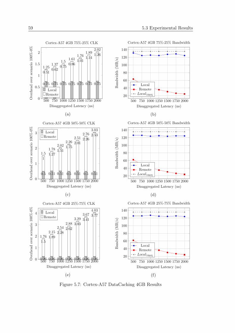
59 5.3 Experimental Results
500 750 1000 1250 1500 1750 20000
0.5
1
1.5
2
1.251.37
1.51.61
1.761.89
2.02
0.510.62
0.750.86
1.011.14
1.26
0.75 0.75 0.75 0.75 0.75 0.75 0.75
Disaggregated Latency (ns)
Ove
rhea
dov
ersc
enar
io10
0%-0
%
Cortex-A57 4GB 75%-25% CLK
LocalRemote
(a)
500 750 1000 1250 1500 1750 2000
20
40
60
80
100
120
140
Disaggregated Latency (ns)
Ban
dw
idth
(MB
/s)
Cortex-A57 4GB 75%-25% Bandwidth
LocalRemoteLocal100%
(b)
500 750 1000 1250 1500 1750 20000
1
2
3
1.51.78
2.022.26
2.512.76
3.03
11.27
1.511.75
2.012.26
2.53
0.5 0.51 0.51 0.5 0.51 0.5 0.51
Disaggregated Latency (ns)
Ove
rhea
dov
ersc
enar
io10
0%-0
%
Cortex-A57 4GB 50%-50% CLK
LocalRemote
(c)
500 750 1000 1250 1500 1750 2000
20
40
60
80
100
120
140
Disaggregated Latency (ns)
Ban
dw
idth
(MB
/s)
Cortex-A57 4GB 50%-50% Bandwidth
LocalRemoteLocal100%
(d)
500 750 1000 1250 1500 1750 20000
1
2
3
4
1.762.15
2.542.88
3.293.67
4.03
1.51.89
2.282.62
3.033.41
3.77
0.26 0.26 0.26 0.26 0.26 0.26 0.26
Disaggregated Latency (ns)
Ove
rhea
dov
ersc
enar
io10
0%-0
%
Cortex-A57 4GB 25%-75% CLK
LocalRemote
(e)
500 750 1000 1250 1500 1750 2000
20
40
60
80
100
120
140
Disaggregated Latency (ns)
Ban
dw
idth
(MB
/s)
Cortex-A57 4GB 25%-75% Bandwidth
LocalRemoteLocal100%
(f)
Figure 5.7: Cortex-A57 DataCaching 4GB Results

5. EVALUATION AND EXPERIMENTAL RESULTS 60
500 750 1000 1250 1500 1750 20000
0.5
1
1.16 1.17 1.19 1.19 1.25 1.29 1.33
0.3 0.31 0.34 0.34 0.41 0.44 0.49
0.86 0.86 0.86 0.86 0.83 0.85 0.85
Disaggregated Latency (ns)
Ove
rhea
dov
ersc
enar
io10
0%-0
%Power 8 8GB 75%-25% CLK
LocalRemote
(a)
500 750 1000 1250 1500 1750 200012
14
16
18
20
22
24
Disaggregated Latency (ns)
Ban
dw
idth
(MB
/s)
Power 8 8GB 75%-25% Bandwidth
LocalRemoteLocal100%
(b)
500 750 1000 1250 1500 1750 20000
0.5
11.04
1.15 1.19 1.23 1.28 1.3 1.35
0.560.68 0.71 0.74 0.77 0.81 0.85
0.48 0.47 0.49 0.49 0.5 0.49 0.5
Disaggregated Latency (ns)
Ove
rhea
dov
ersc
enar
io10
0%-0
%
Power 8 8GB 50%-50% CLK
LocalRemote
(c)
500 750 1000 1250 1500 1750 200012
14
16
18
20
22
24
Disaggregated Latency (ns)
Ban
dw
idth
(MB
/s)
Power 8 8GB 50%-50% Bandwidth
LocalRemoteLocal100%
(d)
500 750 1000 1250 1500 1750 20000
0.5
1
1.5
2
1.18 1.2 1.24 1.281.42 1.47
1.91
0.9 0.94 0.99 1.041.16 1.22
1.59
0.28 0.26 0.25 0.25 0.25 0.25 0.32
Disaggregated Latency (ns)
Ove
rhea
dov
ersc
enar
io10
0%-0
%
Power 8 8GB 25%-75% CLK
LocalRemote
(e)
500 750 1000 1250 1500 1750 2000
12
14
16
18
20
22
24
Disaggregated Latency (ns)
Ban
dw
idth
(MB
/s)
Power 8 8GB 25%-75% Bandwidth
LocalRemoteLocal100%
(f)
Figure 5.8: Power 8 DataCaching 8GB Results
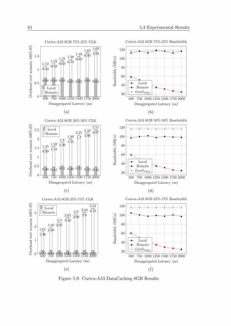
61 5.3 Experimental Results
500 750 1000 1250 1500 1750 20000
0.5
1
1.5
1.121.22
1.31 1.381.48
1.621.69
0.430.53
0.63 0.730.83
0.931.04
0.68 0.68 0.68 0.65 0.65 0.68 0.65
Disaggregated Latency (ns)
Ove
rhea
dov
ersc
enar
io10
0%-0
%
Cortex-A53 8GB 75%-25% CLK
LocalRemote
(a)
500 750 1000 1250 1500 1750 2000
20
40
60
80
100
120
Disaggregated Latency (ns)
Ban
dw
idth
(MB
/s)
Cortex-A53 8GB 75%-25% Bandwidth
LocalRemoteLocal100%
(b)
500 750 1000 1250 1500 1750 20000
0.5
1
1.5
2
2.5
1.451.58
1.81.99
2.212.32
2.51
0.991.14
1.291.51
1.71.86
2.07
0.46 0.44 0.51 0.48 0.51 0.45 0.44
Disaggregated Latency (ns)
Ove
rhea
dov
ersc
enar
io10
0%-0
%
Cortex-A53 8GB 50%-50% CLK
LocalRemote
(c)
500 750 1000 1250 1500 1750 2000
20
40
60
80
100
120
Disaggregated Latency (ns)
Ban
dw
idth
(MB
/s)
Cortex-A53 8GB 50%-50% Bandwidth
LocalRemoteLocal100%
(d)
500 750 1000 1250 1500 1750 20000
1
2
3
1.611.93
2.3
2.652.9 3.04
3.34
1.361.69
2.07
2.422.66 2.8
3.12
0.25 0.24 0.23 0.22 0.25 0.24 0.22
Disaggregated Latency (ns)
Ove
rhea
dov
ersc
enar
io10
0%-0
%
Cortex-A53 8GB 25%-75% CLK
LocalRemote
(e)
500 750 1000 1250 1500 1750 2000
20
40
60
80
100
120
Disaggregated Latency (ns)
Ban
dw
idth
(MB
/s)
Cortex-A53 8GB 25%-75% Bandwidth
LocalRemoteLocal100%
(f)
Figure 5.9: Cortex-A53 DataCaching 8GB Results
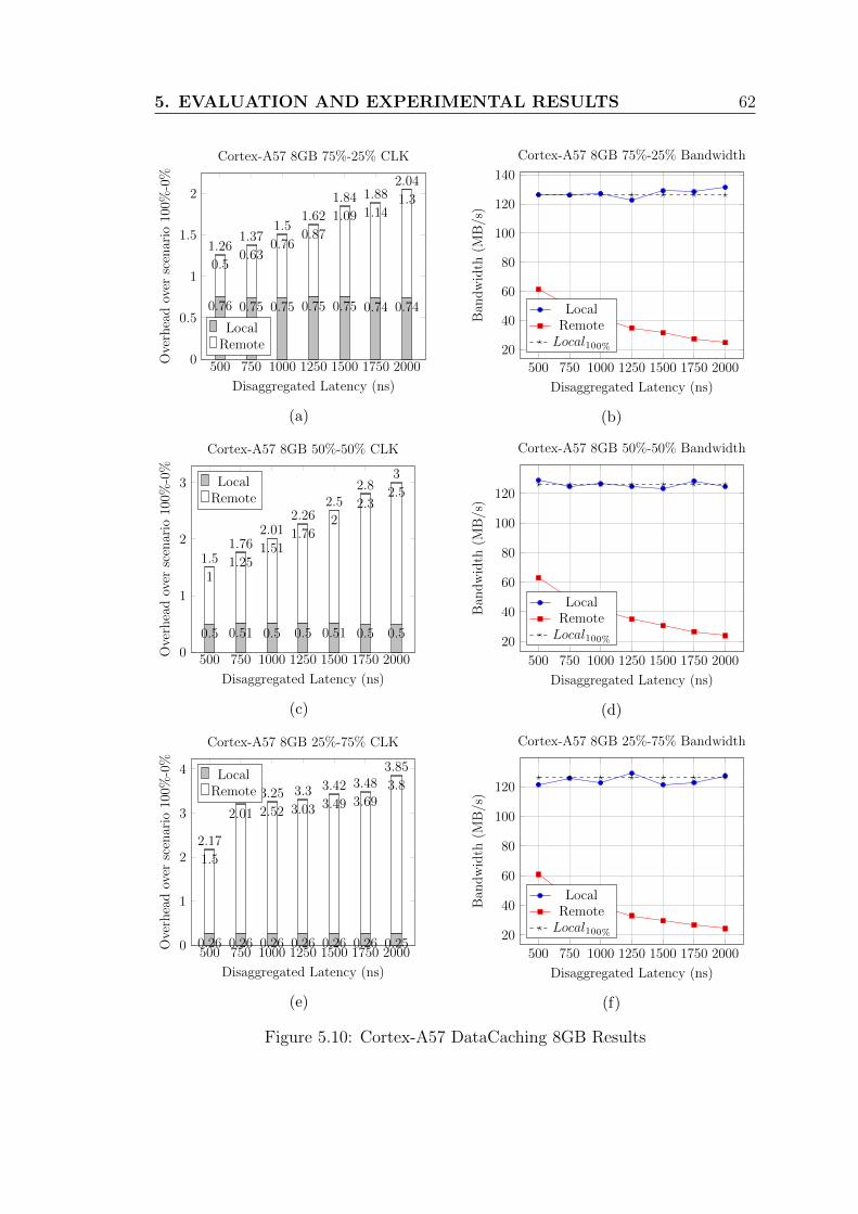
5. EVALUATION AND EXPERIMENTAL RESULTS 62
500 750 1000 1250 1500 1750 20000
0.5
1
1.5
2
1.261.37
1.51.62
1.84 1.882.04
0.50.63
0.760.87
1.09 1.141.3
0.76 0.75 0.75 0.75 0.75 0.74 0.74
Disaggregated Latency (ns)
Ove
rhea
dov
ersc
enar
io10
0%-0
%Cortex-A57 8GB 75%-25% CLK
LocalRemote
(a)
500 750 1000 1250 1500 1750 2000
20
40
60
80
100
120
140
Disaggregated Latency (ns)
Ban
dw
idth
(MB
/s)
Cortex-A57 8GB 75%-25% Bandwidth
LocalRemoteLocal100%
(b)
500 750 1000 1250 1500 1750 20000
1
2
3
1.51.76
2.012.26
2.52.8
3
11.25
1.511.76
22.3
2.5
0.5 0.51 0.5 0.5 0.51 0.5 0.5
Disaggregated Latency (ns)
Ove
rhea
dov
ersc
enar
io10
0%-0
%
Cortex-A57 8GB 50%-50% CLK
LocalRemote
(c)
500 750 1000 1250 1500 1750 2000
20
40
60
80
100
120
Disaggregated Latency (ns)
Ban
dw
idth
(MB
/s)
Cortex-A57 8GB 50%-50% Bandwidth
LocalRemoteLocal100%
(d)
500 750 1000 1250 1500 1750 20000
1
2
3
4
2.17
3.2 3.25 3.3 3.42 3.483.85
1.5
2.01 2.52 3.03 3.49 3.693.8
0.26 0.26 0.26 0.26 0.26 0.26 0.25
Disaggregated Latency (ns)
Ove
rhea
dov
ersc
enar
io10
0%-0
%
Cortex-A57 8GB 25%-75% CLK
LocalRemote
(e)
500 750 1000 1250 1500 1750 2000
20
40
60
80
100
120
Disaggregated Latency (ns)
Ban
dw
idth
(MB
/s)
Cortex-A57 8GB 25%-75% Bandwidth
LocalRemoteLocal100%
(f)
Figure 5.10: Cortex-A57 DataCaching 8GB Results
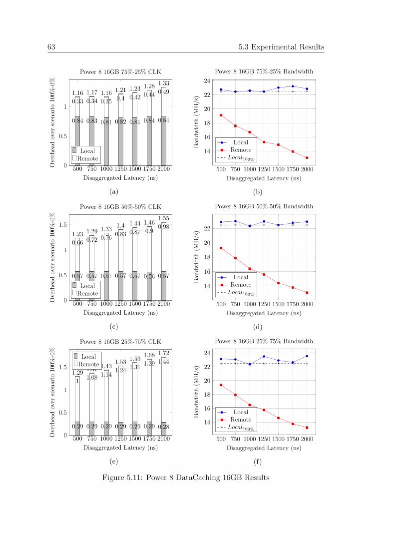
63 5.3 Experimental Results
500 750 1000 1250 1500 1750 20000
0.5
1
1.16 1.17 1.16 1.21 1.23 1.28 1.33
0.33 0.34 0.35 0.4 0.42 0.44 0.49
0.84 0.83 0.81 0.82 0.81 0.84 0.84
Disaggregated Latency (ns)
Ove
rhea
dov
ersc
enar
io10
0%-0
%
Power 8 16GB 75%-25% CLK
LocalRemote
(a)
500 750 1000 1250 1500 1750 2000
14
16
18
20
22
24
Disaggregated Latency (ns)
Ban
dw
idth
(MB
/s)
Power 8 16GB 75%-25% Bandwidth
LocalRemoteLocal100%
(b)
500 750 1000 1250 1500 1750 20000
0.5
1
1.5
1.23 1.29 1.331.4 1.44 1.46
1.55
0.66 0.72 0.760.83 0.87 0.9
0.98
0.57 0.57 0.57 0.57 0.57 0.56 0.57
Disaggregated Latency (ns)
Ove
rhea
dov
ersc
enar
io10
0%-0
%
Power 8 16GB 50%-50% CLK
LocalRemote
(c)
500 750 1000 1250 1500 1750 2000
14
16
18
20
22
Disaggregated Latency (ns)
Ban
dw
idth
(MB
/s)
Power 8 16GB 50%-50% Bandwidth
LocalRemoteLocal100%
(d)
500 750 1000 1250 1500 1750 20000
0.5
1
1.51.29
1.37 1.431.53 1.59
1.68 1.72
11.08 1.14
1.24 1.311.39 1.44
0.29 0.29 0.29 0.29 0.29 0.29 0.28
Disaggregated Latency (ns)
Ove
rhea
dov
ersc
enar
io10
0%-0
%
Power 8 16GB 25%-75% CLK
LocalRemote
(e)
500 750 1000 1250 1500 1750 2000
14
16
18
20
22
24
Disaggregated Latency (ns)
Ban
dw
idth
(MB
/s)
Power 8 16GB 25%-75% Bandwidth
LocalRemoteLocal100%
(f)
Figure 5.11: Power 8 DataCaching 16GB Results
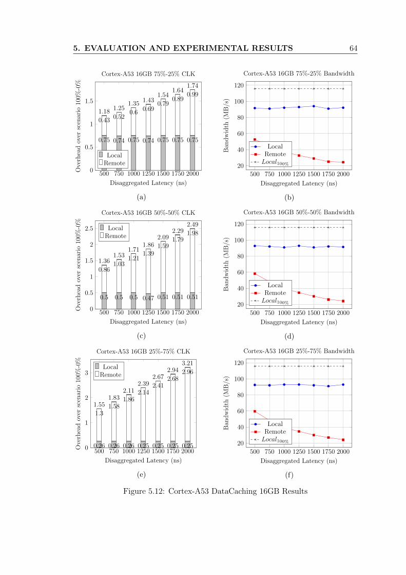
5. EVALUATION AND EXPERIMENTAL RESULTS 64
500 750 1000 1250 1500 1750 20000
0.5
1
1.5
1.181.25
1.351.43
1.541.64
1.74
0.430.52
0.60.69
0.790.89
0.99
0.75 0.74 0.75 0.74 0.75 0.75 0.75
Disaggregated Latency (ns)
Ove
rhea
dov
ersc
enar
io10
0%-0
%Cortex-A53 16GB 75%-25% CLK
LocalRemote
(a)
500 750 1000 1250 1500 1750 2000
20
40
60
80
100
120
Disaggregated Latency (ns)
Ban
dw
idth
(MB
/s)
Cortex-A53 16GB 75%-25% Bandwidth
LocalRemoteLocal100%
(b)
500 750 1000 1250 1500 1750 20000
0.5
1
1.5
2
2.5
1.361.53
1.711.86
2.092.29
2.49
0.861.03
1.211.39
1.591.79
1.98
0.5 0.5 0.5 0.47 0.51 0.51 0.51
Disaggregated Latency (ns)
Ove
rhea
dov
ersc
enar
io10
0%-0
%
Cortex-A53 16GB 50%-50% CLK
LocalRemote
(c)
500 750 1000 1250 1500 1750 2000
20
40
60
80
100
120
Disaggregated Latency (ns)
Ban
dw
idth
(MB
/s)
Cortex-A53 16GB 50%-50% Bandwidth
LocalRemoteLocal100%
(d)
500 750 1000 1250 1500 1750 20000
1
2
3
1.551.83
2.112.39
2.672.94
3.21
1.31.58
1.862.14
2.412.68
2.96
0.26 0.26 0.26 0.25 0.25 0.25 0.25
Disaggregated Latency (ns)
Ove
rhea
dov
ersc
enar
io10
0%-0
%
Cortex-A53 16GB 25%-75% CLK
LocalRemote
(e)
500 750 1000 1250 1500 1750 2000
20
40
60
80
100
120
Disaggregated Latency (ns)
Ban
dw
idth
(MB
/s)
Cortex-A53 16GB 25%-75% Bandwidth
LocalRemoteLocal100%
(f)
Figure 5.12: Cortex-A53 DataCaching 16GB Results
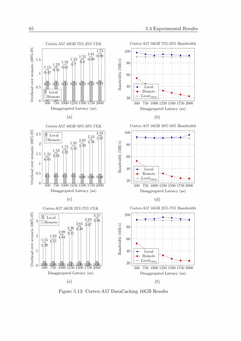
65 5.3 Experimental Results
500 750 1000 1250 1500 1750 20000
0.5
1
1.5
1.131.23
1.321.42
1.521.61
1.73
0.420.52
0.610.7
0.80.89
0.99
0.71 0.71 0.71 0.72 0.72 0.72 0.74
Disaggregated Latency (ns)
Ove
rhea
dov
ersc
enar
io10
0%-0
%
Cortex-A57 16GB 75%-25% CLK
LocalRemote
(a)
500 750 1000 1250 1500 1750 2000
20
40
60
80
100
Disaggregated Latency (ns)
Ban
dw
idth
(MB
/s)
Cortex-A57 16GB 75%-25% Bandwidth
LocalRemoteLocal100%
(b)
500 750 1000 1250 1500 1750 20000
0.5
1
1.5
2
2.5
1.351.53
1.721.91
2.052.24
2.42
0.851.04
1.221.41
1.591.78
1.97
0.5 0.5 0.5 0.5 0.46 0.46 0.46
Disaggregated Latency (ns)
Ove
rhea
dov
ersc
enar
io10
0%-0
%
Cortex-A57 16GB 50%-50% CLK
LocalRemote
(c)
500 750 1000 1250 1500 1750 200020
40
60
80
100
Disaggregated Latency (ns)
Ban
dw
idth
(MB
/s)
Cortex-A57 16GB 50%-50% Bandwidth
LocalRemoteLocal100%
(d)
500 750 1000 1250 1500 1750 20000
1
2
3
1.551.82
2.092.36
2.652.93
3.21
1.291.57
1.842.11
2.392.67
2.95
0.26 0.26 0.26 0.25 0.26 0.26 0.26
Disaggregated Latency (ns)
Ove
rhea
dov
ersc
enar
io10
0%-0
%
Cortex-A57 16GB 25%-75% CLK
LocalRemote
(e)
500 750 1000 1250 1500 1750 200020
40
60
80
100
Disaggregated Latency (ns)
Ban
dw
idth
(MB
/s)
Cortex-A57 16GB 25%-75% Bandwidth
LocalRemoteLocal100%
(f)
Figure 5.13: Cortex-A57 DataCaching 16GB Results

5. EVALUATION AND EXPERIMENTAL RESULTS 66
500 750 1000 1250 1500 1750 20000
0.5
1
1.22 1.24 1.27 1.29 1.31 1.32 1.33
0.34 0.37 0.4 0.41 0.44 0.45 0.46
0.87 0.87 0.87 0.87 0.87 0.87 0.87
Disaggregated Latency (ns)
Ove
rhea
dov
ersc
enar
io10
0%-0
%Power 8 32GB 75%-25% CLK
LocalRemote
(a)
500 750 1000 1250 1500 1750 200012
14
16
18
20
22
24
Disaggregated Latency (ns)
Ban
dw
idth
(MB
/s)
Power 8 32GB 75%-25% Bandwidth
LocalRemoteLocal100%
(b)
500 750 1000 1250 1500 1750 20000
0.5
1
1.51.27 1.32 1.38 1.44 1.49 1.54 1.59
0.68 0.73 0.8 0.85 0.9 0.95 1
0.59 0.59 0.59 0.59 0.59 0.59 0.59
Disaggregated Latency (ns)
Ove
rhea
dov
ersc
enar
io10
0%-0
%
Power 8 32GB 50%-50% CLK
LocalRemote
(c)
500 750 1000 1250 1500 1750 200012
14
16
18
20
22
24
Disaggregated Latency (ns)
Ban
dw
idth
(MB
/s)
Power 8 32GB 50%-50% Bandwidth
LocalRemoteLocal100%
(d)
500 750 1000 1250 1500 1750 20000
0.5
1
1.51.33
1.41.48
1.571.65
1.731.8
1.031.11
1.181.27
1.351.43
1.51
0.3 0.3 0.3 0.3 0.3 0.3 0.3
Disaggregated Latency (ns)
Ove
rhea
dov
ersc
enar
io10
0%-0
%
Power 8 32GB 25%-75% CLK
LocalRemote
(e)
500 750 1000 1250 1500 1750 200012
14
16
18
20
22
24
Disaggregated Latency (ns)
Ban
dw
idth
(MB
/s)
Power 8 32GB 25%-75% Bandwidth
LocalRemoteLocal100%
(f)
Figure 5.14: Power 8 DataCaching 32GB Results
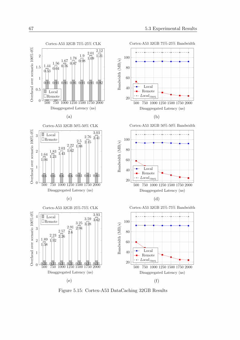
67 5.3 Experimental Results
500 750 1000 1250 1500 1750 20000
0.5
1
1.5
2
1.441.56
1.671.78
1.92.01
2.12
0.530.64
0.760.87
0.981.09
1.21
0.91 0.91 0.91 0.91 0.91 0.91 0.92
Disaggregated Latency (ns)
Ove
rhea
dov
ersc
enar
io10
0%-0
%
Cortex-A53 32GB 75%-25% CLK
LocalRemote
(a)
500 750 1000 1250 1500 1750 200020
40
60
80
100
Disaggregated Latency (ns)
Ban
dw
idth
(MB
/s)
Cortex-A53 32GB 75%-25% Bandwidth
LocalRemoteLocal100%
(b)
500 750 1000 1250 1500 1750 20000
1
2
3
1.641.83
2.032.22
2.52.76
3.03
1.041.23
1.431.62
1.882.15
2.41
0.6 0.6 0.6 0.6 0.61 0.61 0.61
Disaggregated Latency (ns)
Ove
rhea
dov
ersc
enar
io10
0%-0
%
Cortex-A53 32GB 50%-50% CLK
LocalRemote
(c)
500 750 1000 1250 1500 1750 200020
40
60
80
100
Disaggregated Latency (ns)
Ban
dw
idth
(MB
/s)
Cortex-A53 32GB 50%-50% Bandwidth
LocalRemoteLocal100%
(d)
500 750 1000 1250 1500 1750 20000
1
2
3
4
1.892.23
2.572.91
3.253.59
3.93
1.581.92
2.262.6
2.943.28
3.62
0.31 0.31 0.31 0.31 0.31 0.31 0.31
Disaggregated Latency (ns)
Ove
rhea
dov
ersc
enar
io10
0%-0
%
Cortex-A53 32GB 25%-75% CLK
LocalRemote
(e)
500 750 1000 1250 1500 1750 200020
40
60
80
100
Disaggregated Latency (ns)
Ban
dw
idth
(MB
/s)
Cortex-A53 32GB 25%-75% Bandwidth
LocalRemoteLocal100%
(f)
Figure 5.15: Cortex-A53 DataCaching 32GB Results
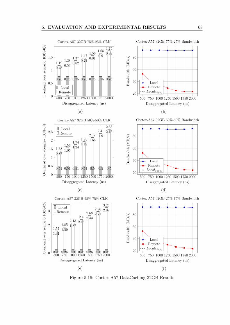
5. EVALUATION AND EXPERIMENTAL RESULTS 68
500 750 1000 1250 1500 1750 20000
0.5
1
1.5
1.191.28
1.371.47
1.561.65
1.75
0.430.53
0.620.71
0.810.9
0.99
0.75 0.75 0.75 0.75 0.75 0.75 0.76
Disaggregated Latency (ns)
Ove
rhea
dov
ersc
enar
io10
0%-0
%Cortex-A57 32GB 75%-25% CLK
LocalRemote
(a)
500 750 1000 1250 1500 1750 2000
20
40
60
80
Disaggregated Latency (ns)
Ban
dw
idth
(MB
/s)
Cortex-A57 32GB 75%-25% Bandwidth
LocalRemoteLocal100%
(b)
500 750 1000 1250 1500 1750 20000
0.5
1
1.5
2
2.5
1.381.56
1.741.93
2.172.41
2.65
0.871.05
1.241.42
1.661.9
2.15
0.51 0.51 0.51 0.51 0.5 0.5 0.5
Disaggregated Latency (ns)
Ove
rhea
dov
ersc
enar
io10
0%-0
%
Cortex-A57 32GB 50%-50% CLK
LocalRemote
(c)
500 750 1000 1250 1500 1750 200020
40
60
80
Disaggregated Latency (ns)
Ban
dw
idth
(MB
/s)
Cortex-A57 32GB 50%-50% Bandwidth
LocalRemoteLocal100%
(d)
500 750 1000 1250 1500 1750 20000
1
2
3
1.571.85
2.132.4
2.682.96
3.24
1.311.59
1.872.15
2.432.71
2.99
0.26 0.26 0.26 0.26 0.26 0.26 0.26
Disaggregated Latency (ns)
Ove
rhea
dov
ersc
enar
io10
0%-0
%
Cortex-A57 32GB 25%-75% CLK
LocalRemote
(e)
500 750 1000 1250 1500 1750 200020
40
60
80
Disaggregated Latency (ns)
Ban
dw
idth
(MB
/s)
Cortex-A57 32GB 25%-75% Bandwidth
LocalRemoteLocal100%
(f)
Figure 5.16: Cortex-A57 DataCaching 32GB Results
CHAPTER6Conclusion and Future Work
6.1 Conclusion
In conclusion we can support that we have developed a simple Disaggregated
Memory System Simulator in combination with Orion Papadakis thesis[26]. Our
both approach comes with a simplistic level of detail, so that it can depict the
Disaggregated Memory System behavior, in an approximate way. It, also, bears
the Intel Pin framework and DRAMSim2 coupling. Despite the fact that the
coupling result comes along with a large overhead, it is useful for future work and
study on Memory System Simulators. It can play a supporting role as a base in
Disaggregated Memory System Simulators, due to the fact that a Simulator like
the DiMEM Simulator has never developed before, not even in a simplistic way.
Regarding to the experimental methods, we can say that only one approach
was used, due to the nature of the Benchmark. To simulate in a sampling way over
a benchmark application, the profile knowledge is very important. Sampling with
Nyquist theorem may be more safe, accurate and reliable, than the more custom
way. However the custom way sampling is not meaningless. In the current thesis
approach we observed that the chosen sampling method was accurate.
6. CONCLUSION AND FUTURE WORK 70
Furthermore, we observe that the Disaggregated Memory System behavior is
quite depicted, either in the Latency, or in the Bandwidth results. The higher
Disaggregated latency we give to the DiMEM Simulator, the clock grows, and the
bandwidth falls.
Comparing a system with Disaggregated Memory with a Local-only one in
Instruction and Memory Access level, the Disaggregated Memory shows worse
results than the Local, because of the Disaggregated Latency overhead. Despite
that fact, in our evaluation approach, we can observe the existence of a point,
where the results are not so bad. At the point of Disaggregated Latency = 1000 ns,
where the Step is 2x increased, we can see that the Bandwidth does not present the
linear 0.5x attended fall, but it is better than that. Consequently, we can assume
that while the Disaggregated Latency is bellow 1000ns, we can use Disaggregated
Memory without paying for the Disaggregated Latency in the highest price, which
is the 0.5x of the performance.
One more important observation is that despite the size of a the simulated
memory, it is very important the simulated application to be limited in the same
size from the system, otherwise we will collect wrong results.
Finally, it must be noticed, that only a high-level evaluation approach (for
example in application level) can provide us with a clear answer about when a
Disaggregated System presents a better performance than the traditional orga-
nization. In future work, we propose some ideas for further and more detailed
Disaggregated Systems evaluation.

71 6.2 Future Work
6.2 Future Work
The combined work of this thesis with the Orion Papadakis’ ones[26] leads us to
the following common conclusions:
1. Study of the Disaggregated Memory System benefits in an application level.
A transparent to application memory interface is needed. That study can
be done using criteria like Quality of Service (QoS) in an application level
comparison between Local-only Memory System and Local-Disaggregated
Memory System.
2. Main Memory Access Dynamic Split to Local and Remote Memory. The
dynamic memory access split can be achieved by implementing an algorithm
which passes a memory access to local or remote using a Memory Mapping
scheme.
3. Further study and experimentation with more DRAMSim2 parameters. In-
clude the ITLB namespace on the Simulator, as well as the I(nstruction)
Cache Levels
4. Experimentation with another DRAM Simulators. Ramulator[18] may be
a suitable one due to the reason that it is self-presented as the Memory
Simulator with the lower run time (2.5x faster than the next fastest simulator
and 2.7x faster than DRAMSim2).
5. Experimentation with latest Memory Technologies. 3D-stacked DRAM stud-
ies are aiming to overcome the traditional DRAM limits. The lights are on
the Hybrid Memory Cube (HMC) which is a type of 3D-stacked DRAM be-
cause of its usability for server systems and processing-in-memory (PIM) ar-

6. CONCLUSION AND FUTURE WORK 72
chitecture. HMC-Sim2.0[19] and CasHMC[14] Simulators have been designed
for this technology with CasHMC being a step forward due to its cycle ac-
curate HMC modeling. Regarding to the latest Memory technologies exper-
imentation, the DiMEM Simulator can be easily upgraded to them, through
a simple DRAMSim2 library replacement, for example with CasHMC li-
brary/interface. There is no need of changing the simulation feeding process,
except from the update() and addTransaction() library functions which must
be replaced by the corresponding new library ones.
6. Further DiMEM Simulator development/expansion by implementing new
modules alongside the already existed. These modules may be pools con-
taining different kind of resources such as FPGAs, GPUs, Accelerators, as
well as, more advanced interconnects between them.
7. More detailed evaluation of the used evaluation methods. Since, Raytrace
benchmark had been sampled in specific areas, the question of which is the
result reliability by using random sampling, in the same benchmark, was
risen.
8. Find a way to overcome docker container constraints to simulate more Cloud-
suite benchmarks.

73 6.2 Future Work
APPENDICES
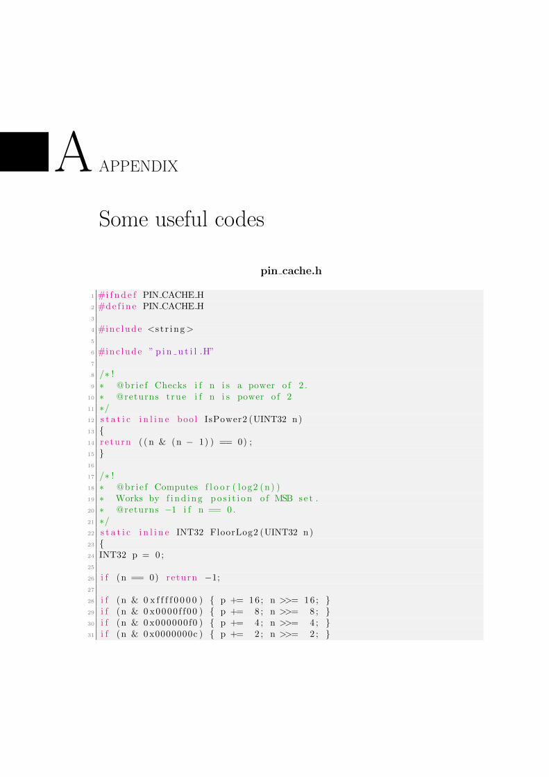
AAPPENDIX
Some useful codes
pin cache.h
1 #i f n d e f PIN CACHE H2 #de f i n e PIN CACHE H3
4 #inc lude <s t r i ng>5
6 #inc lude ” p i n u t i l .H”7
8 /∗ !9 ∗ @brie f Checks i f n i s a power o f 2 .
10 ∗ @returns t rue i f n i s power o f 211 ∗/12 s t a t i c i n l i n e bool IsPower2 (UINT32 n)13 {14 re turn ( ( n & (n − 1) ) == 0) ;15 }16
17 /∗ !18 ∗ @brie f Computes f l o o r ( log2 (n) )19 ∗ Works by f i nd i n g po s i t i o n o f MSB se t .20 ∗ @returns −1 i f n == 0 .21 ∗/22 s t a t i c i n l i n e INT32 FloorLog2 (UINT32 n)23 {24 INT32 p = 0 ;25
26 i f (n == 0) re turn −1;27
28 i f (n & 0 x f f f f 0 0 0 0 ) { p += 16 ; n >>= 16 ; }29 i f (n & 0 x0000 f f00 ) { p += 8 ; n >>= 8 ; }30 i f (n & 0x000000f0 ) { p += 4 ; n >>= 4 ; }31 i f (n & 0x0000000c ) { p += 2 ; n >>= 2 ; }

75
32 i f (n & 0x00000002 ) { p += 1 ; }33
34 re turn p ;35 }36
37 /∗ !38 ∗ @brie f Computes f l o o r ( log2 (n) )39 ∗ Works by f i nd i n g po s i t i o n o f MSB se t .40 ∗ @returns −1 i f n == 0 .41 ∗/42 s t a t i c i n l i n e INT32 Cei lLog2 (UINT32 n)43 {44 re turn FloorLog2 (n − 1) + 1 ;45 }46
47 /∗ !48 ∗ @brie f Cache tag − s e l f c l e a r i n g on c r e a t i on49 ∗/50 c l a s s CACHETAG51 {52 pr i va t e :53 ADDRINT tag ;54
55 pub l i c :56 CACHETAG(ADDRINT tag = 0) { tag = tag ; }57 bool operator==(const CACHETAG &r i gh t ) const { re turn tag == r i gh t .
tag ; }58 operator ADDRINT( ) const { re turn tag ; }59 } ;60
61
62 /∗ !63 ∗ Everything r e l a t e d to cache s e t s64 ∗/65 namespace CACHE SET66 {67
68 /∗ !69 ∗ @brie f Cache s e t d i r e c t mapped70 ∗/71 c l a s s DIRECTMAPPED72 {73 pr i va t e :74 CACHETAG tag ;75
76 pub l i c :77 DIRECTMAPPED(UINT32 a s s o c i a t i v i t y = 1) { ASSERTX( a s s o c i a t i v i t y == 1)
; }
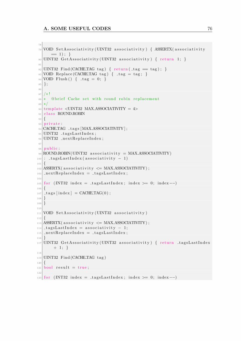
A. SOME USEFUL CODES 76
78
79 VOID Se tA s s o c i a t i v i t y (UINT32 a s s o c i a t i v i t y ) { ASSERTX( a s s o c i a t i v i t y== 1) ; }
80 UINT32 GetAs soc i a t i v i t y (UINT32 a s s o c i a t i v i t y ) { re turn 1 ; }81
82 UINT32 Find (CACHETAG tag ) { re turn ( tag == tag ) ; }83 VOID Replace (CACHETAG tag ) { tag = tag ; }84 VOID Flush ( ) { tag = 0 ; }85 } ;86
87 /∗ !88 ∗ @brie f Cache s e t with round rob in replacement89 ∗/90 template <UINT32 MAX ASSOCIATIVITY = 4>91 c l a s s ROUNDROBIN92 {93 pr i va t e :94 CACHETAG tag s [MAX ASSOCIATIVITY ] ;95 UINT32 tagsLas t Index ;96 UINT32 nextReplaceIndex ;97
98 pub l i c :99 ROUNDROBIN(UINT32 a s s o c i a t i v i t y = MAX ASSOCIATIVITY)
100 : t agsLas t Index ( a s s o c i a t i v i t y − 1)101 {102 ASSERTX( a s s o c i a t i v i t y <= MAX ASSOCIATIVITY) ;103 nextReplaceIndex = tagsLas t Index ;104
105 f o r ( INT32 index = tagsLas t Index ; index >= 0 ; index−−)106 {107 t a g s [ index ] = CACHETAG(0) ;108 }109 }110
111 VOID Se tA s s o c i a t i v i t y (UINT32 a s s o c i a t i v i t y )112 {113 ASSERTX( a s s o c i a t i v i t y <= MAX ASSOCIATIVITY) ;114 tagsLas t Index = a s s o c i a t i v i t y − 1 ;115 nextReplaceIndex = tagsLas t Index ;116 }117 UINT32 GetAs soc i a t i v i t y (UINT32 a s s o c i a t i v i t y ) { re turn tagsLas t Index
+ 1 ; }118
119 UINT32 Find (CACHETAG tag )120 {121 bool r e s u l t = true ;122
123 f o r ( INT32 index = tagsLas t Index ; index >= 0 ; index−−)

77
124 {125 // t h i s i s an ugly micro−opt imizat ion , but i t does cause a126 // t i g h t e r assembly loop f o r ARM that way . . .127 i f ( t a g s [ index ] == tag ) goto end ;128 }129 r e s u l t = f a l s e ;130
131 end : re turn r e s u l t ;132 }133
134 VOID Replace (CACHETAG tag )135 {136 // g++ −O3 too dumb to do CSE on f o l l ow i n g l i n e s ? !137 const UINT32 index = nextReplaceIndex ;138
139 t a g s [ index ] = tag ;140 // cond i t i on t y p i c a l l y f a s t e r than modulo141 nextReplaceIndex = ( index == 0 ? tagsLas t Index : index − 1) ;142 }143 VOID Flush ( )144 {145 f o r ( INT32 index = tagsLas t Index ; index >= 0 ; index−−)146 {147 t a g s [ index ] = 0 ;148 }149 nextReplaceIndex= tagsLas t Index ;150 }151 } ;152
153 } // namespace CACHE SET154
155 namespace CACHEALLOC156 {157 typede f enum158 {159 STORE ALLOCATE,160 STORE NO ALLOCATE161 } STORE ALLOCATION;162 }163
164 /∗ !165 ∗ @brie f Generic cache base c l a s s ; no a l l o c a t e s p e c i a l i z a t i o n , no
cache s e t s p e c i a l i z a t i o n166 ∗/167 c l a s s CACHE BASE168 {169 pub l i c :170 // types , cons tant s

A. SOME USEFUL CODES 78
171 typede f enum172 {173 ACCESS TYPE LOAD,174 ACCESS TYPE STORE,175 ACCESS TYPE NUM176 } ACCESS TYPE;177
178 protec ted :179 s t a t i c const UINT32 HIT MISS NUM = 2 ;180 CACHE STATS a c c e s s [ACCESS TYPE NUM] [ HIT MISS NUM ] ;181
182 pr i va t e :183 // input params184 const std : : s t r i n g name ;185 const UINT32 cacheS i z e ;186 const UINT32 l i n e S i z e ;187 const UINT32 a s s o c i a t i v i t y ;188 UINT32 numberOfFlushes ;189 UINT32 numberOfResets ;190
191 // computed params192 const UINT32 l i n e S h i f t ;193 const UINT32 setIndexMask ;194
195 CACHE STATS SumAccess ( bool h i t ) const196 {197 CACHE STATS sum = 0 ;198
199 f o r (UINT32 accessType = 0 ; accessType < ACCESS TYPE NUM; accessType++)
200 {201 sum += ac c e s s [ accessType ] [ h i t ] ;202 }203
204 re turn sum ;205 }206
207 protec ted :208 UINT32 NumSets ( ) const { re turn setIndexMask + 1 ; }209
210 pub l i c :211 // con s t ru c t o r s / d e s t r u c t o r s212 CACHE BASE( std : : s t r i n g name , UINT32 cacheSize , UINT32 l i n e S i z e ,
UINT32 a s s o c i a t i v i t y ) ;213
214 // a c c e s s o r s215 UINT32 CacheSize ( ) const { re turn cacheS i z e ; }216 UINT32 L ineS i z e ( ) const { re turn l i n e S i z e ; }

79
217 UINT32 As s o c i a t i v i t y ( ) const { re turn a s s o c i a t i v i t y ; }218 //219 CACHE STATS Hits (ACCESS TYPE accessType ) const { re turn a c c e s s [
accessType ] [ t rue ] ; }220 CACHE STATS Misses (ACCESS TYPE accessType ) const { re turn a c c e s s [
accessType ] [ f a l s e ] ; }221 CACHE STATS Accesses (ACCESS TYPE accessType ) const { re turn Hits (
accessType ) + Misses ( accessType ) ;}222 CACHE STATS Hits ( ) const { re turn SumAccess ( t rue ) ;}223 CACHE STATS Misses ( ) const { re turn SumAccess ( f a l s e ) ;}224 CACHE STATS Accesses ( ) const { re turn Hits ( ) + Misses ( ) ;}225
226 CACHE STATS Flushes ( ) const { re turn numberOfFlushes ;}227 CACHE STATS Resets ( ) const { re turn numberOfResets ;}228
229 VOID Spl i tAddres s ( const ADDRINT addr , CACHETAG & tag , UINT32 &set Index ) const
230 {231 tag = addr >> l i n e S h i f t ;232 se t Index = tag & setIndexMask ;233 }234
235 VOID Spl i tAddres s ( const ADDRINT addr , CACHETAG & tag , UINT32 &setIndex , UINT32 & l i n e Index ) const
236 {237 const UINT32 lineMask = l i n e S i z e − 1 ;238 l i n e Index = addr & lineMask ;239 Sp l i tAddres s ( addr , tag , s e t Index ) ;240 }241
242 VOID IncFlushCounter ( )243 {244 numberOfFlushes += 1 ;245 }246
247 VOID IncResetCounter ( )248 {249 numberOfResets += 1 ;250 }251
252 std : : ostream & StatsLong ( std : : ostream & out ) const ;253 } ;254
255 CACHE BASE : :CACHE BASE( std : : s t r i n g name , UINT32 cacheSize , UINT32l i n e S i z e , UINT32 a s s o c i a t i v i t y )
256 : name (name) ,257 ca cheS i z e ( cacheS i ze ) ,258 l i n e S i z e ( l i n e S i z e ) ,

A. SOME USEFUL CODES 80
259 a s s o c i a t i v i t y ( a s s o c i a t i v i t y ) ,260 l i n e S h i f t ( FloorLog2 ( l i n e S i z e ) ) ,261 setIndexMask ( ( cacheS i ze / ( a s s o c i a t i v i t y ∗ l i n e S i z e ) ) − 1)262 {263
264 ASSERTX( IsPower2 ( l i n e S i z e ) ) ;265 ASSERTX( IsPower2 ( setIndexMask + 1) ) ;266
267 f o r (UINT32 accessType = 0 ; accessType < ACCESS TYPE NUM; accessType++)
268 {269 a c c e s s [ accessType ] [ f a l s e ] = 0 ;270 a c c e s s [ accessType ] [ t rue ] = 0 ;271 }272 }273
274 /∗ !275 ∗ @brie f S ta t s output method276 ∗/277 std : : ostream & CACHE BASE : : StatsLong ( std : : ostream & out ) const278 {279 const UINT32 headerWidth = 19 ;280 const UINT32 numberWidth = 10 ;281
282 out << name << ” : ” << std : : endl ;283
284 f o r (UINT32 i = 0 ; i < ACCESS TYPE NUM; i++)285 {286 const ACCESS TYPE accessType = ACCESS TYPE( i ) ;287
288 std : : s t r i n g type ( accessType == ACCESS TYPE LOAD ? ”Load” : ” Store ” ) ;289
290 out << S t r i ngS t r i n g ( type + ” Hits : ” , headerWidth )291 << S t r i ng In t ( Hits ( accessType ) , numberWidth ) << std : : endl ;292 out << S t r i ngS t r i n g ( type + ” Misses : ” , headerWidth )293 << S t r i ng In t ( Misses ( accessType ) , numberWidth ) << std : : endl ;294 out << S t r i ngS t r i n g ( type + ” Accesses : ” , headerWidth )295 << S t r i ng In t ( Accesses ( accessType ) , numberWidth ) << std : : endl ;296 out << S t r i ngS t r i n g ( type + ” Miss Rate : ” , headerWidth )297 << St r i ngF l t (100 . 0 ∗ Misses ( accessType ) / Accesses ( accessType ) , 2 ,
numberWidth−1) << ”%” << std : : endl ;298 out << std : : endl ;299 }300
301 out << S t r i ngS t r i n g ( ”Total Hits : ” , headerWidth , ’ ’ )302 << S t r i ng In t ( Hits ( ) , numberWidth ) << std : : endl ;303 out << S t r i ngS t r i n g ( ”Total Misses : ” , headerWidth , ’ ’ )304 << S t r i ng In t ( Misses ( ) , numberWidth ) << std : : endl ;

81
305 out << S t r i ngS t r i n g ( ”Total Accesses : ” , headerWidth , ’ ’ )306 << S t r i ng In t ( Accesses ( ) , numberWidth ) << std : : endl ;307 out << S t r i ngS t r i n g ( ”Total Miss Rate : ” , headerWidth , ’ ’ )308 << St r i ngF l t (100 . 0 ∗ Misses ( ) / Accesses ( ) , 2 , numberWidth−1) << ”%”
<< std : : endl ;309
310 out << S t r i ngS t r i n g ( ”Flushes : ” , headerWidth , ’ ’ )311 << S t r i ng In t ( Flushes ( ) , numberWidth ) << std : : endl ;312 out << S t r i ngS t r i n g ( ” Stat Resets : ” , headerWidth , ’ ’ )313 << S t r i ng In t ( Resets ( ) , numberWidth ) << std : : endl ;314
315 out << std : : endl ;316
317 re turn out ;318 }319
320 /// ostream operator f o r CACHE BASE321 std : : ostream & operator<< ( std : : ostream & out , const CACHE BASE &
cacheBase )322 {323 re turn cacheBase . StatsLong ( out ) ;324 }325
326 /∗ !327 ∗ @brie f Templated cache c l a s s with s p e c i f i c cache s e t a l l o c a t i o n
p o l i c i e s328 ∗329 ∗ Al l that remains to be done here i s a l l o c a t e and d e a l l o c a t e the
r i g h t330 ∗ type o f cache s e t s .331 ∗/332 template <c l a s s SET, UINT32 MAX SETS, UINT32 STORE ALLOCATION>333 c l a s s CACHE : pub l i c CACHE BASE334 {335 pr i va t e :336 SET s e t s [MAX SETS ] ;337
338 pub l i c :339 // con s t ru c t o r s / d e s t r u c t o r s340 CACHE( std : : s t r i n g name , UINT32 cacheSize , UINT32 l i n e S i z e , UINT32
a s s o c i a t i v i t y )341 : CACHE BASE(name , cacheSize , l i n e S i z e , a s s o c i a t i v i t y )342 {343 ASSERTX(NumSets ( ) <= MAX SETS) ;344
345 f o r (UINT32 i = 0 ; i < NumSets ( ) ; i++)346 {347 s e t s [ i ] . S e tA s s o c i a t i v i t y ( a s s o c i a t i v i t y ) ;
A. SOME USEFUL CODES 82
348 }349 }350
351 // mod i f i e r s352 /// Cache ac c e s s from addr to addr+s i z e −1353 bool Access (ADDRINT addr , UINT32 s i z e , ACCESS TYPE accessType ) ;354 /// Cache ac c e s s at addr that does not span cache l i n e s355 bool Acce s sS ing l eL ine (ADDRINT addr , ACCESS TYPE accessType ) ;356 void Flush ( ) ;357 void ResetStat s ( ) ;358 } ;359
360 /∗ !361 ∗ @return true i f a l l a c ce s s ed cache l i n e s h i t362 ∗/363
364 template <c l a s s SET, UINT32 MAX SETS, UINT32 STORE ALLOCATION>365 bool CACHE<SET,MAX SETS,STORE ALLOCATION> : : Access (ADDRINT addr ,
UINT32 s i z e , ACCESS TYPE accessType )366 {367 const ADDRINT highAddr = addr + s i z e ;368 bool a l l H i t = true ;369
370 const ADDRINT l i n e S i z e = LineS i z e ( ) ;371 const ADDRINT notLineMask = ˜( l i n e S i z e − 1) ;372 do373 {374 CACHETAG tag ;375 UINT32 set Index ;376
377 Sp l i tAddres s ( addr , tag , s e t Index ) ;378
379 SET & se t = s e t s [ s e t Index ] ;380
381 bool l o c a lH i t = s e t . Find ( tag ) ;382 a l lH i t &= l o c a lH i t ;383
384 // on miss , l oads always a l l o c a t e , s t o r e s op t i o na l l y385 i f ( ( ! l o c a lH i t ) && ( accessType == ACCESS TYPE LOAD | |
STORE ALLOCATION == CACHEALLOC: : STOREALLOCATE) )386 {387 s e t . Replace ( tag ) ;388 }389
390 addr = ( addr & notLineMask ) + l i n e S i z e ; // s t a r t o f next cache l i n e391 }392 whi le ( addr < highAddr ) ;393
83
394 a c c e s s [ accessType ] [ a l l H i t ]++;395
396 re turn a l lH i t ;397 }398
399 /∗ !400 ∗ @return true i f a cce s s ed cache l i n e h i t s401 ∗/402 template <c l a s s SET, UINT32 MAX SETS, UINT32 STORE ALLOCATION>403 bool CACHE<SET,MAX SETS,STORE ALLOCATION> : : Acce s sS ing l eL ine (ADDRINT
addr , ACCESS TYPE accessType )404 {405 CACHETAG tag ;406 UINT32 set Index ;407
408 Sp l i tAddres s ( addr , tag , s e t Index ) ;409
410 SET & se t = s e t s [ s e t Index ] ;411
412 bool h i t = s e t . Find ( tag ) ;413
414 // on miss , l oads always a l l o c a t e , s t o r e s op t i o na l l y415 i f ( ( ! h i t ) && ( accessType == ACCESS TYPE LOAD | | STORE ALLOCATION
== CACHEALLOC: : STOREALLOCATE) )416 {417 s e t . Replace ( tag ) ;418 }419
420 a c c e s s [ accessType ] [ h i t ]++;421
422 re turn h i t ;423 }424 /∗ !425 ∗ @return true i f a cce s s ed cache l i n e h i t s426 ∗/427 template <c l a s s SET, UINT32 MAX SETS, UINT32 STORE ALLOCATION>428 void CACHE<SET,MAX SETS,STORE ALLOCATION> : : Flush ( )429 {430 f o r ( INT32 index = NumSets ( ) ; index >= 0 ; index−−) {431 SET & se t = s e t s [ index ] ;432 s e t . Flush ( ) ;433 }434 IncFlushCounter ( ) ;435 }436
437 template <c l a s s SET, UINT32 MAX SETS, UINT32 STORE ALLOCATION>438 void CACHE<SET,MAX SETS,STORE ALLOCATION> : : ResetStat s ( )439 {
A. SOME USEFUL CODES 84
440 f o r (UINT32 accessType = 0 ; accessType < ACCESS TYPE NUM; accessType++)
441 {442 a c c e s s [ accessType ] [ f a l s e ] = 0 ;443 a c c e s s [ accessType ] [ t rue ] = 0 ;444 }445 IncResetCounter ( ) ;446 }447
448
449 // de f i n e sho r t cu t s450 #de f i n e CACHE DIRECTMAPPED(MAX SETS, ALLOCATION) CACHE<CACHE SET : :
DIRECTMAPPED, MAX SETS, ALLOCATION>451 #de f i n e CACHE ROUNDROBIN(MAX SETS, MAX ASSOCIATIVITY, ALLOCATION)
CACHE<CACHE SET : :ROUND ROBIN<MAX ASSOCIATIVITY>, MAX SETS,ALLOCATION>
452
453 #end i f // PIN CACHE H
boost/preprocessor/iteration/local.hpp
1 # /∗ ∗∗∗∗∗∗∗∗∗∗∗∗∗∗∗∗∗∗∗∗∗∗∗∗∗∗∗∗∗∗∗∗∗∗∗∗∗∗∗∗∗∗∗∗∗∗∗∗∗∗∗∗∗∗∗∗∗∗∗∗∗∗∗2 # ∗ (C) Copyright Paul Mensonides 2002 .3 # ∗ Dis t r ibu t ed under the Boost Software License , Vers ion 1 . 0 .4 # ∗ ( See accompanying f i l e LICENSE 1 0 . txt or copy at5 # ∗ http : //www. boost . org /LICENSE 1 0 . txt )6 # ∗∗∗∗∗∗∗∗∗∗∗∗∗∗∗∗∗∗∗∗∗∗∗∗∗∗∗∗∗∗∗∗∗∗∗∗∗∗∗∗∗∗∗∗∗∗∗∗∗∗∗∗∗∗∗∗∗∗∗∗∗∗∗ ∗/7 #8 # /∗ See http ://www. boost . org f o r most r e c ent ve r s i on . ∗/9 #
10 # i f n d e f BOOST PREPROCESSOR ITERATION LOCAL HPP11 # de f i n e BOOST PREPROCESSOR ITERATION LOCAL HPP12 #13 # inc lude <boost / p r ep ro c e s s o r / c on f i g / c on f i g . hpp>14 # inc lude <boost / p r ep ro c e s s o r / s l o t / s l o t . hpp>15 # inc lude <boost / p r ep ro c e s s o r / tup l e /elem . hpp>16 #17 # /∗ BOOST PP LOCAL ITERATE ∗/18 #19 # de f i n e BOOST PP LOCAL ITERATE( ) <boost / p r ep ro c e s s o r / i t e r a t i o n /
d e t a i l / l o c a l . hpp>20 #
85
21 # de f i n e BOOST PP LOCAL C(n) (BOOST PP LOCAL S) <= n && (BOOST PP LOCAL F) >= n
22 # de f i n e BOOST PP LOCAL R(n) (BOOST PP LOCAL F) <= n && (BOOST PP LOCAL S) >= n
23 #24 # end i f

BAPPENDIX
Simulation output
The Simulation Output consists of two discrete output files: Pintool’s .out file and
DRAMSim2 .log file.
Pintool .out file
These files contain information about Ram accesses and their percentage per Win-
dow, the Local and Disaggregated Clock cycles, the Total and Total Instrumented
Instructions, the Local and Disaggregated Cycles per Instruction (CPI) and finaly
a complete Cache report. The Cache report contains information about Load/S-
tore/Total Hits, Misses, Accesses, Miss Rate for each Cache Level separately. A
simple example is following:
1 Ram Accesses : 629850
2 Ram Percentage : 0.31%
3 Simulat ion number : 1 o f 10
4 ============================
5
6 Ram Accesses : 634720
7 Ram Percentage : 0.32%
8 Simulat ion number : 2 o f 10
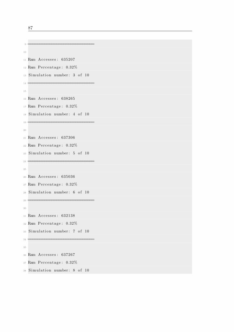
87
9 ============================
10
11 Ram Accesses : 635207
12 Ram Percentage : 0.32%
13 Simulat ion number : 3 o f 10
14 ============================
15
16 Ram Accesses : 638265
17 Ram Percentage : 0.32%
18 Simulat ion number : 4 o f 10
19 ============================
20
21 Ram Accesses : 637306
22 Ram Percentage : 0.32%
23 Simulat ion number : 5 o f 10
24 ============================
25
26 Ram Accesses : 635036
27 Ram Percentage : 0.32%
28 Simulat ion number : 6 o f 10
29 ============================
30
31 Ram Accesses : 632138
32 Ram Percentage : 0.32%
33 Simulat ion number : 7 o f 10
34 ============================
35
36 Ram Accesses : 637267
37 Ram Percentage : 0.32%
38 Simulat ion number : 8 o f 10
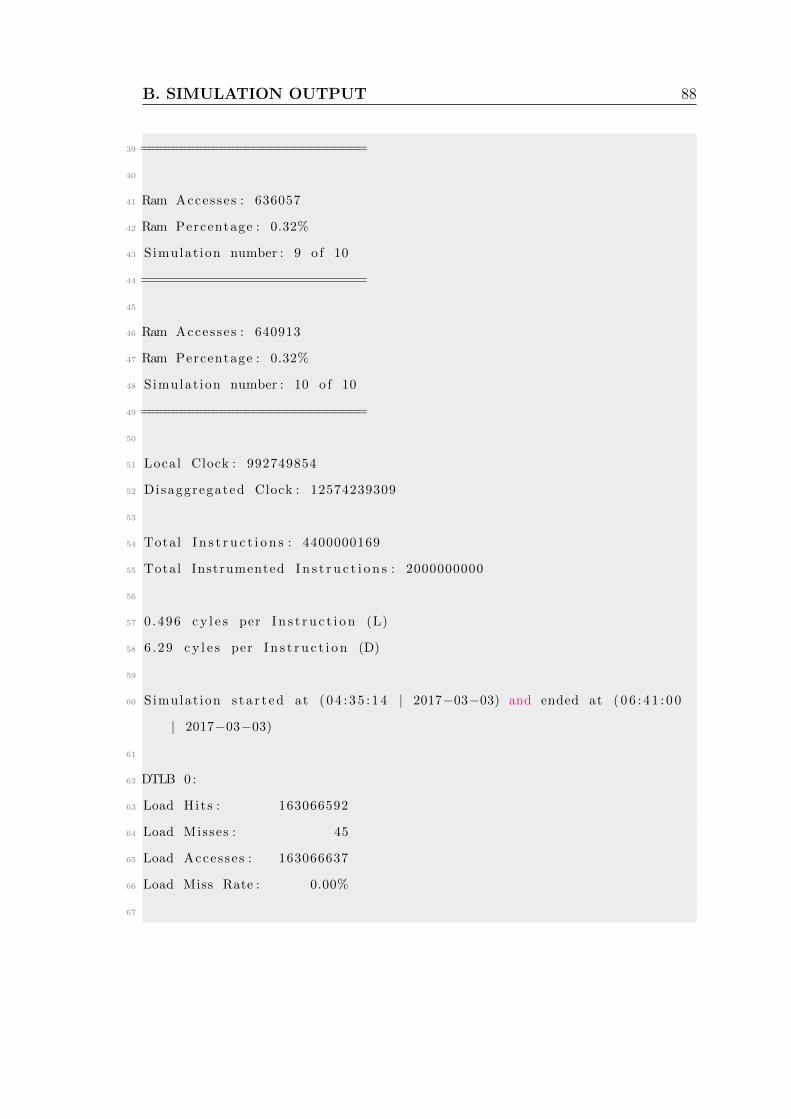
B. SIMULATION OUTPUT 88
39 ============================
40
41 Ram Accesses : 636057
42 Ram Percentage : 0.32%
43 Simulat ion number : 9 o f 10
44 ============================
45
46 Ram Accesses : 640913
47 Ram Percentage : 0.32%
48 Simulat ion number : 10 o f 10
49 ============================
50
51 Local Clock : 992749854
52 Disaggregated Clock : 12574239309
53
54 Total I n s t r u c t i o n s : 4400000169
55 Total Instrumented I n s t r u c t i o n s : 2000000000
56
57 0 .496 c y l e s per I n s t r u c t i o n (L)
58 6 .29 c y l e s per I n s t r u c t i o n (D)
59
60 Simulat ion s t a r t ed at ( 0 4 : 3 5 : 1 4 | 2017−03−03) and ended at ( 0 6 : 4 1 : 0 0
| 2017−03−03)
61
62 DTLB 0 :
63 Load Hits : 163066592
64 Load Misses : 45
65 Load Accesses : 163066637
66 Load Miss Rate : 0.00%
67
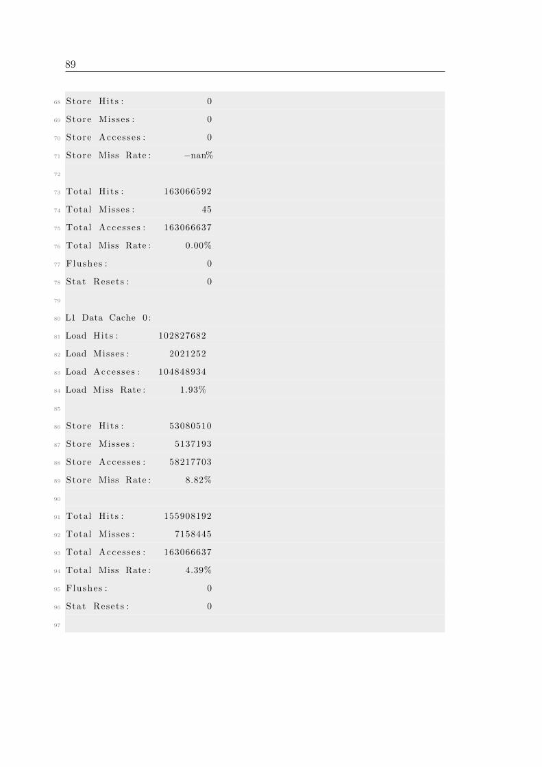
89
68 Store Hits : 0
69 Store Misses : 0
70 Store Accesses : 0
71 Store Miss Rate : −nan%
72
73 Total Hits : 163066592
74 Total Misses : 45
75 Total Accesses : 163066637
76 Total Miss Rate : 0.00%
77 Flushes : 0
78 Stat Resets : 0
79
80 L1 Data Cache 0 :
81 Load Hits : 102827682
82 Load Misses : 2021252
83 Load Accesses : 104848934
84 Load Miss Rate : 1.93%
85
86 Store Hits : 53080510
87 Store Misses : 5137193
88 Store Accesses : 58217703
89 Store Miss Rate : 8.82%
90
91 Total Hits : 155908192
92 Total Misses : 7158445
93 Total Accesses : 163066637
94 Total Miss Rate : 4.39%
95 Flushes : 0
96 Stat Resets : 0
97
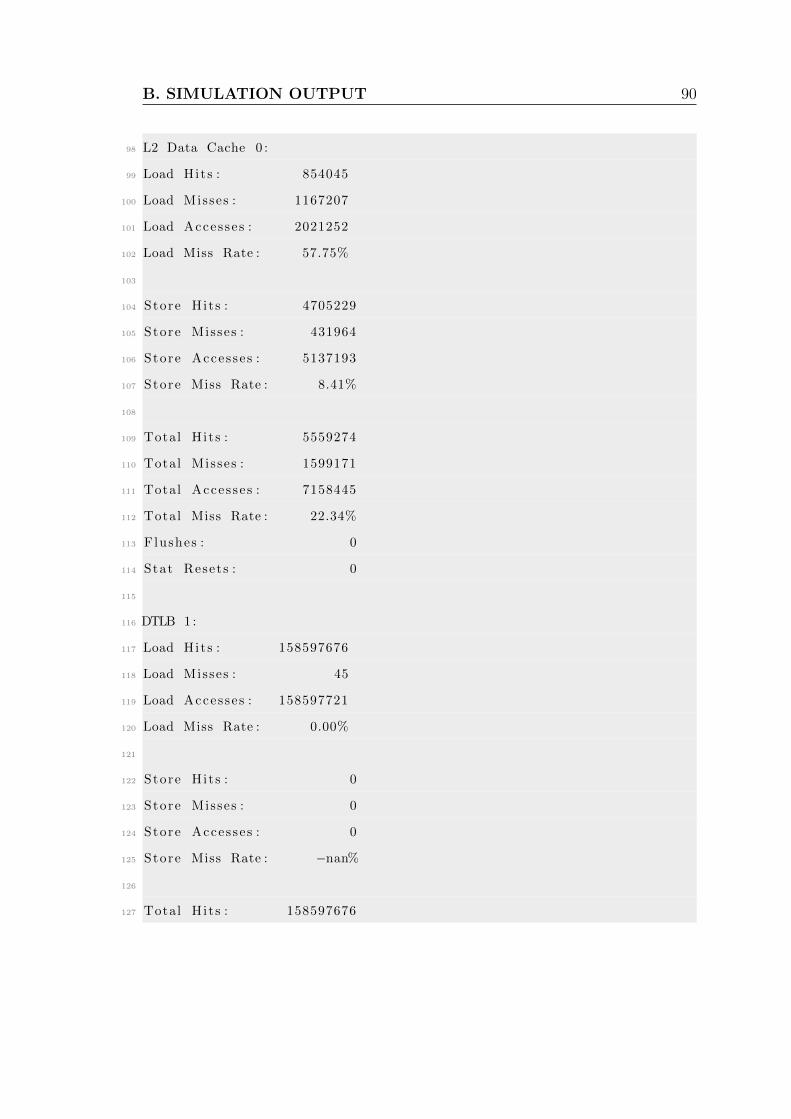
B. SIMULATION OUTPUT 90
98 L2 Data Cache 0 :
99 Load Hits : 854045
100 Load Misses : 1167207
101 Load Accesses : 2021252
102 Load Miss Rate : 57.75%
103
104 Store Hits : 4705229
105 Store Misses : 431964
106 Store Accesses : 5137193
107 Store Miss Rate : 8.41%
108
109 Total Hits : 5559274
110 Total Misses : 1599171
111 Total Accesses : 7158445
112 Total Miss Rate : 22.34%
113 Flushes : 0
114 Stat Resets : 0
115
116 DTLB 1 :
117 Load Hits : 158597676
118 Load Misses : 45
119 Load Accesses : 158597721
120 Load Miss Rate : 0.00%
121
122 Store Hits : 0
123 Store Misses : 0
124 Store Accesses : 0
125 Store Miss Rate : −nan%
126
127 Total Hits : 158597676
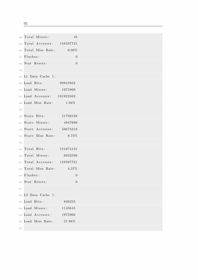
91
128 Total Misses : 45
129 Total Accesses : 158597721
130 Total Miss Rate : 0.00%
131 Flushes : 0
132 Stat Resets : 0
133
134 L1 Data Cache 1 :
135 Load Hits : 99947603
136 Load Misses : 1975900
137 Load Accesses : 101923503
138 Load Miss Rate : 1.94%
139
140 Store Hits : 51726528
141 Store Misses : 4947690
142 Store Accesses : 56674218
143 Store Miss Rate : 8.73%
144
145 Total Hits : 151674131
146 Total Misses : 6923590
147 Total Accesses : 158597721
148 Total Miss Rate : 4.37%
149 Flushes : 0
150 Stat Resets : 0
151
152 L2 Data Cache 1 :
153 Load Hits : 830255
154 Load Misses : 1145645
155 Load Accesses : 1975900
156 Load Miss Rate : 57.98%
157
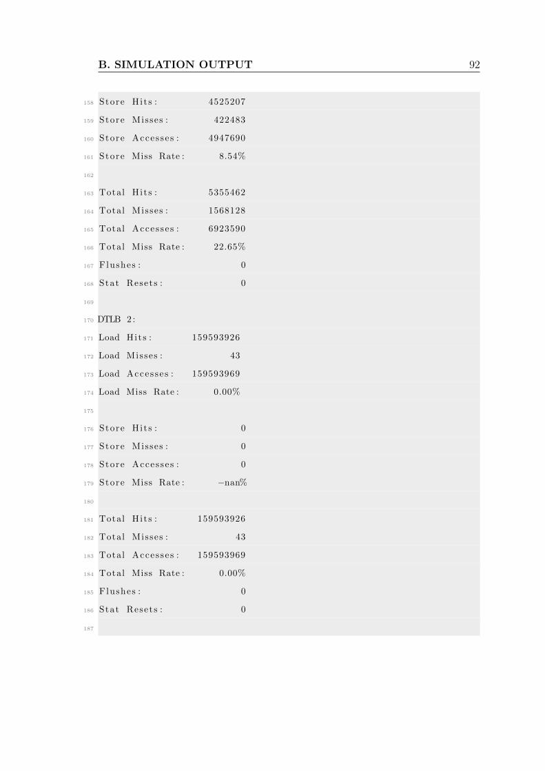
B. SIMULATION OUTPUT 92
158 Store Hits : 4525207
159 Store Misses : 422483
160 Store Accesses : 4947690
161 Store Miss Rate : 8.54%
162
163 Total Hits : 5355462
164 Total Misses : 1568128
165 Total Accesses : 6923590
166 Total Miss Rate : 22.65%
167 Flushes : 0
168 Stat Resets : 0
169
170 DTLB 2 :
171 Load Hits : 159593926
172 Load Misses : 43
173 Load Accesses : 159593969
174 Load Miss Rate : 0.00%
175
176 Store Hits : 0
177 Store Misses : 0
178 Store Accesses : 0
179 Store Miss Rate : −nan%
180
181 Total Hits : 159593926
182 Total Misses : 43
183 Total Accesses : 159593969
184 Total Miss Rate : 0.00%
185 Flushes : 0
186 Stat Resets : 0
187
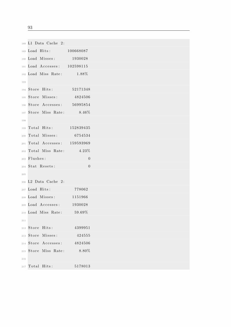
93
188 L1 Data Cache 2 :
189 Load Hits : 100668087
190 Load Misses : 1930028
191 Load Accesses : 102598115
192 Load Miss Rate : 1.88%
193
194 Store Hits : 52171348
195 Store Misses : 4824506
196 Store Accesses : 56995854
197 Store Miss Rate : 8.46%
198
199 Total Hits : 152839435
200 Total Misses : 6754534
201 Total Accesses : 159593969
202 Total Miss Rate : 4.23%
203 Flushes : 0
204 Stat Resets : 0
205
206 L2 Data Cache 2 :
207 Load Hits : 778062
208 Load Misses : 1151966
209 Load Accesses : 1930028
210 Load Miss Rate : 59.69%
211
212 Store Hits : 4399951
213 Store Misses : 424555
214 Store Accesses : 4824506
215 Store Miss Rate : 8.80%
216
217 Total Hits : 5178013
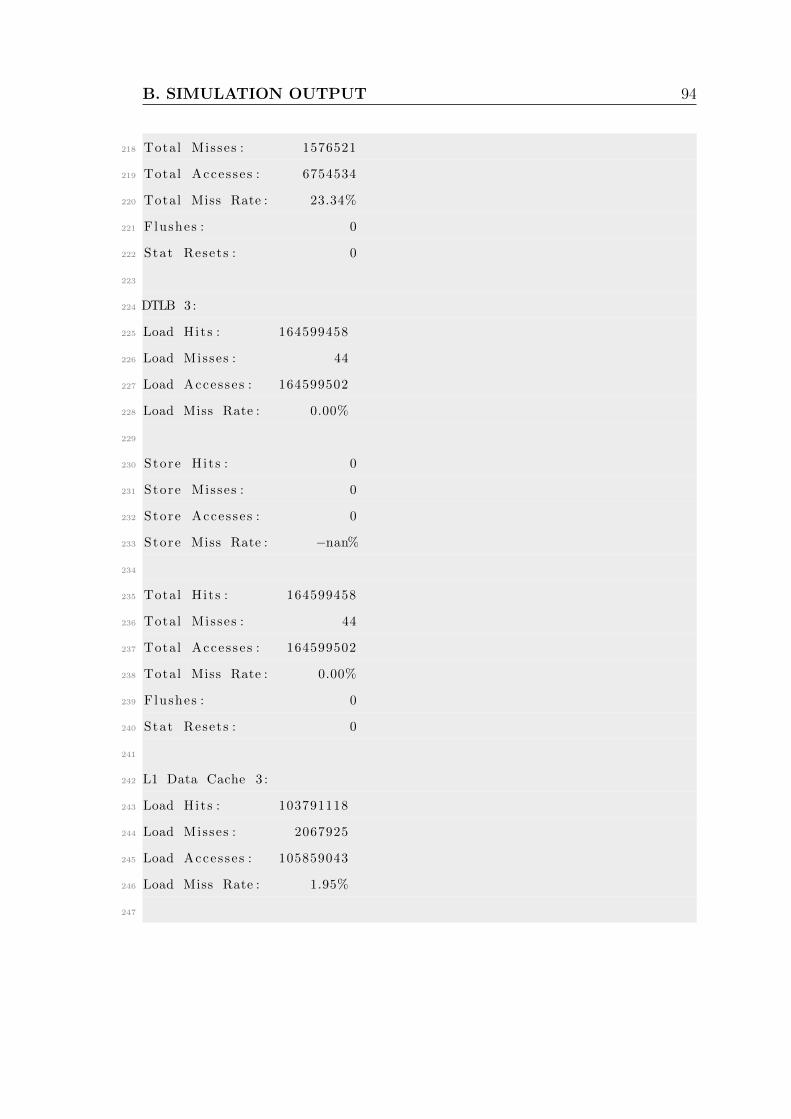
B. SIMULATION OUTPUT 94
218 Total Misses : 1576521
219 Total Accesses : 6754534
220 Total Miss Rate : 23.34%
221 Flushes : 0
222 Stat Resets : 0
223
224 DTLB 3 :
225 Load Hits : 164599458
226 Load Misses : 44
227 Load Accesses : 164599502
228 Load Miss Rate : 0.00%
229
230 Store Hits : 0
231 Store Misses : 0
232 Store Accesses : 0
233 Store Miss Rate : −nan%
234
235 Total Hits : 164599458
236 Total Misses : 44
237 Total Accesses : 164599502
238 Total Miss Rate : 0.00%
239 Flushes : 0
240 Stat Resets : 0
241
242 L1 Data Cache 3 :
243 Load Hits : 103791118
244 Load Misses : 2067925
245 Load Accesses : 105859043
246 Load Miss Rate : 1.95%
247

95
248 Store Hits : 53658600
249 Store Misses : 5081859
250 Store Accesses : 58740459
251 Store Miss Rate : 8.65%
252
253 Total Hits : 157449718
254 Total Misses : 7149784
255 Total Accesses : 164599502
256 Total Miss Rate : 4.34%
257 Flushes : 0
258 Stat Resets : 0
259
260 L2 Data Cache 3 :
261 Load Hits : 885205
262 Load Misses : 1182720
263 Load Accesses : 2067925
264 Load Miss Rate : 57.19%
265
266 Store Hits : 4651640
267 Store Misses : 430219
268 Store Accesses : 5081859
269 Store Miss Rate : 8.47%
270
271 Total Hits : 5536845
272 Total Misses : 1612939
273 Total Accesses : 7149784
274 Total Miss Rate : 22.56%
275 Flushes : 0
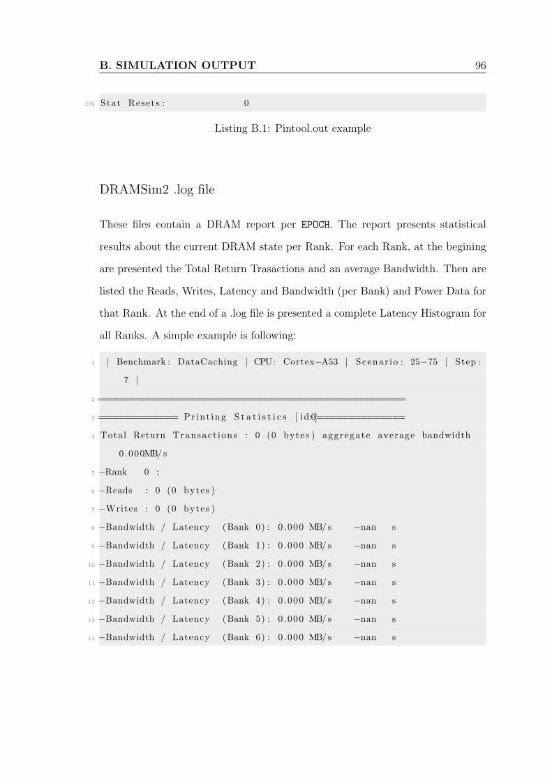
B. SIMULATION OUTPUT 96
276 Stat Resets : 0
Listing B.1: Pintool.out example
DRAMSim2 .log file
These files contain a DRAM report per EPOCH. The report presents statistical
results about the current DRAM state per Rank. For each Rank, at the begining
are presented the Total Return Trasactions and an average Bandwidth. Then are
listed the Reads, Writes, Latency and Bandwidth (per Bank) and Power Data for
that Rank. At the end of a .log file is presented a complete Latency Histogram for
all Ranks. A simple example is following:
1 | Benchmark : DataCaching | CPU: Cortex−A53 | Scenar io : 25−75 | Step :
7 |
2 =======================================================
3 ============== Pr int ing S t a t i s t i c s [ id:0]==============
4 Total Return Transact ions : 0 (0 bytes ) aggregate average bandwidth
0 .000MB/ s
5 −Rank 0 :
6 −Reads : 0 (0 bytes )
7 −Writes : 0 (0 bytes )
8 −Bandwidth / Latency (Bank 0) : 0 .000 MB/ s −nan s
9 −Bandwidth / Latency (Bank 1) : 0 .000 MB/ s −nan s
10 −Bandwidth / Latency (Bank 2) : 0 .000 MB/ s −nan s
11 −Bandwidth / Latency (Bank 3) : 0 .000 MB/ s −nan s
12 −Bandwidth / Latency (Bank 4) : 0 .000 MB/ s −nan s
13 −Bandwidth / Latency (Bank 5) : 0 .000 MB/ s −nan s
14 −Bandwidth / Latency (Bank 6) : 0 .000 MB/ s −nan s

97
15 −Bandwidth / Latency (Bank 7) : 0 .000 MB/ s −nan s
16 −Bandwidth / Latency (Bank 8) : 0 .000 MB/ s −nan s
17 −Bandwidth / Latency (Bank 9) : 0 .000 MB/ s −nan s
18 −Bandwidth / Latency (Bank 10) : 0 .000 MB/ s −nan s
19 −Bandwidth / Latency (Bank 11) : 0 .000 MB/ s −nan s
20 −Bandwidth / Latency (Bank 12) : 0 .000 MB/ s −nan s
21 −Bandwidth / Latency (Bank 13) : 0 .000 MB/ s −nan s
22 −Bandwidth / Latency (Bank 14) : 0 .000 MB/ s −nan s
23 −Bandwidth / Latency (Bank 15) : 0 .000 MB/ s −nan s
24 == Power Data f o r Rank 0
25 Average Power (mW) : 0 .000
26 −Background (mW) : 0 .000
27 −Act/Pre (mW) : 0 .000
28 −Burst (mW) : 0 .000
29 −Refresh (mW) : 0 .000
30
31 == Pending Transact ions : 0 (0 )==
32 ==== Channel [ 0 ] ====
33 | Benchmark : DataCaching | CPU: Cortex−A53 | Scenar io : 25−75 | Step :
7 |
34 =======================================================
35 ============== Pr int ing S t a t i s t i c s [ id:0]==============
36 Total Return Transact ions : 1636284 (104722176 bytes ) aggregate
average bandwidth 118.353MB/ s
37 −Rank 0 :
38 −Reads : 1196027 (76545728 bytes )
39 −Writes : 440257 (28176448 bytes )
40 −Bandwidth / Latency (Bank 0) : 7 .488 MB/ s 34040.604 s
41 −Bandwidth / Latency (Bank 1) : 7 .436 MB/ s 33998.760 s
42 −Bandwidth / Latency (Bank 2) : 7 .410 MB/ s 34029.888 s

B. SIMULATION OUTPUT 98
43 −Bandwidth / Latency (Bank 3) : 7 .356 MB/ s 33996.971 s
44 −Bandwidth / Latency (Bank 4) : 7 .343 MB/ s 34047.424 s
45 −Bandwidth / Latency (Bank 5) : 7 .287 MB/ s 34035.362 s
46 −Bandwidth / Latency (Bank 6) : 7 .350 MB/ s 34057.701 s
47 −Bandwidth / Latency (Bank 7) : 7 .413 MB/ s 34086.468 s
48 −Bandwidth / Latency (Bank 8) : 7 .364 MB/ s 34009.594 s
49 −Bandwidth / Latency (Bank 9) : 7 .425 MB/ s 34010.433 s
50 −Bandwidth / Latency (Bank 10) : 7 .513 MB/ s 34044.460 s
51 −Bandwidth / Latency (Bank 11) : 7 .411 MB/ s 34054.859 s
52 −Bandwidth / Latency (Bank 12) : 7 .378 MB/ s 34092.583 s
53 −Bandwidth / Latency (Bank 13) : 7 .337 MB/ s 34075.726 s
54 −Bandwidth / Latency (Bank 14) : 7 .379 MB/ s 34171.051 s
55 −Bandwidth / Latency (Bank 15) : 7 .464 MB/ s 34069.420 s
56 == Power Data f o r Rank 0
57 Average Power (mW) : 1022.263
58 −Background (mW) : 983.599
59 −Act/Pre (mW) : 13 .160
60 −Burst (mW) : 23 .494
61 −Refresh (mW) : 2 .009
62 −−− Latency l i s t (28)
63 [ l a t ] : #
64 [20−29] : 205
65 [30−39] : 1120626
66 [40−49] : 39903
67 [50−59] : 6047
68 [60−69] : 6657
69 [70−79] : 2554
70 [80−89] : 4143
71 [90−99] : 1732
72 [100−109] : 1427
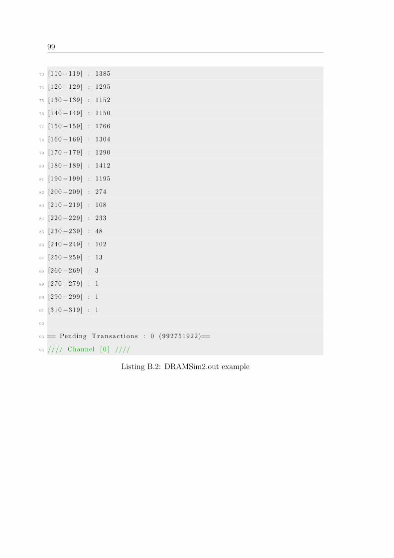
99
73 [110−119] : 1385
74 [120−129] : 1295
75 [130−139] : 1152
76 [140−149] : 1150
77 [150−159] : 1766
78 [160−169] : 1304
79 [170−179] : 1290
80 [180−189] : 1412
81 [190−199] : 1195
82 [200−209] : 274
83 [210−219] : 108
84 [220−229] : 233
85 [230−239] : 48
86 [240−249] : 102
87 [250−259] : 13
88 [260−269] : 3
89 [270−279] : 1
90 [290−299] : 1
91 [310−319] : 1
92
93 == Pending Transact ions : 0 (992751922)==
94 //// Channel [ 0 ] ////
Listing B.2: DRAMSim2.out example

Bibliography
[1] Robert Barnes. “Best Practices for Benchmarking and Performance Analy-
sis in the Cloud (ENT305)”. In: Amazon Web Services, 2013. url: http:
/ / www . slideshare . net / AmazonWebServices / best - practices - for -
benchmarking-and-performance-analysis-in-the-cloud-ent305-aws-
reinvent-2013-28437412?qid=15d7ec92-5db7-48d5-a764-01290a9021c4.
[2] Andrew R Bernat and Barton P Miller. “Anywhere, any-time binary instru-
mentation”. In: Proceedings of the 10th ACM SIGPLAN-SIGSOFT workshop
on Program analysis for software tools. ACM. 2011, pp. 9–16.
[3] Derek Bruening. QZ: Dynamorio: Dynamic instrumentation tool platform.
[4] K Chandrasekaran. Essentials of cloud computing. CRC Press, 2014.
[5] Gal Diskin. “Binary Instrumentation for Security Professionals”. In: Intel.
Blackhat USA (2011).
[6] Robert Demming & Daniel J. Duffy. Introduction to the Boost C++ Li-
braries; Volume I - Foundations. Datasim Education BV, 2010. isbn: 9789491028014.
[7] Karthi Duraisamy and Goutam Das. “WMRD net: An Optical Data Cen-
ter Interconnect”. In: Optical Fiber Communication Conference/National
Fiber Optic Engineers Conference 2013. Optical Society of America, 2013,
101 BIBLIOGRAPHY
OTu3H.3. doi: 10.1364/OFC.2013.OTu3H.3. url: http://www.osapublishing.
org/abstract.cfm?URI=OFC-2013-OTu3H.3.
[8] D. Evdokimov. Light and dark side of code instrumentation. 2013.
[9] Suhaib A Fahmy, Kizheppatt Vipin, and Shanker Shreejith. “Virtualized
FPGA accelerators for efficient cloud computing”. In: Cloud Computing
Technology and Science (CloudCom), 2015 IEEE 7th International Confer-
ence on. IEEE. 2015, pp. 430–435.
[10] Michael Ferdman et al. “Clearing the clouds: a study of emerging scale-out
workloads on modern hardware”. In: ACM SIGPLAN Notices. Vol. 47. 4.
ACM. 2012, pp. 37–48.
[11] Robert E Filman and Klaus Havelund. Source-code instrumentation and
quantification of events. 2002.
[12] Sangjin Han et al. “Network support for resource disaggregation in next-
generation datacenters”. In: Proceedings of the Twelfth ACM Workshop on
Hot Topics in Networks. ACM. 2013, p. 10.
[13] Aamer Jaleel et al. “CMPSim: A Pin-based on-the-fly multi-core cache simu-
lator”. In: Proceedings of the Fourth Annual Workshop on Modeling, Bench-
marking and Simulation (MoBS), co-located with ISCA. 2008, pp. 28–36.
[14] D. I. Jeon and K. S. Chung. “CasHMC: A Cycle-Accurate Simulator for
Hybrid Memory Cube”. In: IEEE Computer Architecture Letters 16.1 (Jan.
2017), pp. 10–13. issn: 1556-6056. doi: 10.1109/LCA.2016.2600601.
BIBLIOGRAPHY 102
[15] Johnls. Dynamic vs. Static Instrumentation @ONLINE. Nov. 2006. url:
https://blogs.msdn.microsoft.com/johnls/2006/11/15/dynamic-vs-
static-instrumentation/.
[16] K. Katrinis et al. “On interconnecting and orchestrating components in
disaggregated data centers: The dReDBox project vision”. In: 2016 Euro-
pean Conference on Networks and Communications (EuCNC). June 2016,
pp. 235–239. doi: 10.1109/EuCNC.2016.7561039.
[17] K. Katrinis et al. “Rack-scale disaggregated cloud data centers: The dReD-
Box project vision”. In: 2016 Design, Automation Test in Europe Conference
Exhibition (DATE). Mar. 2016, pp. 690–695.
[18] Y. Kim, W. Yang, and O. Mutlu. “Ramulator: A Fast and Extensible DRAM
Simulator”. In: IEEE Computer Architecture Letters 15.1 (Jan. 2016), pp. 45–
49. issn: 1556-6056. doi: 10.1109/LCA.2015.2414456.
[19] J. D. Leidel and Y. Chen. “HMC-Sim-2.0: A Simulation Platform for Ex-
ploring Custom Memory Cube Operations”. In: 2016 IEEE International
Parallel and Distributed Processing Symposium Workshops (IPDPSW). May
2016, pp. 621–630. doi: 10.1109/IPDPSW.2016.43.
[20] Kevin Lim et al. “Disaggregated memory for expansion and sharing in blade
servers”. In: ACM SIGARCH Computer Architecture News. Vol. 37. 3. ACM.
2009, pp. 267–278.
[21] Kevin Lim et al. “System-level implications of disaggregated memory”. In:
High Performance Computer Architecture (HPCA), 2012 IEEE 18th Inter-
national Symposium on. IEEE. 2012, pp. 1–12.
103 BIBLIOGRAPHY
[22] Chi-Keung Luk et al. “Pin: building customized program analysis tools with
dynamic instrumentation”. In: Acm sigplan notices. Vol. 40. 6. ACM. 2005,
pp. 190–200.
[23] Hugo Meyer et al. “Disaggregated Computing. An Evaluation of Current
Trends for Datacentres”. In: Procedia Computer Science 108 (2017), pp. 685–
694.
[24] Nicholas Nethercote and Julian Seward. “Valgrind: A program supervision
framework”. In: Electronic notes in theoretical computer science 89.2 (2003),
pp. 44–66.
[25] Tapti Palit, Yongming Shen, and Michael Ferdman. “Demystifying cloud
benchmarking”. In: Performance Analysis of Systems and Software (ISPASS),
2016 IEEE International Symposium on. IEEE. 2016, pp. 122–132.
[26] Orion Papadakis. Memory System Evaluation of Disaggregated High Perfor-
mance Parallel Systems. 2017.
[27] Vijay Janapa Reddi et al. “PIN: A Binary Instrumentation Tool for Com-
puter Architecture Research and Education”. In: Proceedings of the 2004
Workshop on Computer Architecture Education: Held in Conjunction with
the 31st International Symposium on Computer Architecture. WCAE ’04.
Munich, Germany: ACM, 2004. isbn: 978-1-4503-4733-4. doi: 10.1145/
1275571.1275600. url: http://doi.acm.org/10.1145/1275571.1275600.
[28] Paul Rosenfeld, Elliott Cooper-Balis, and Bruce Jacob. “DRAMSim2: A cy-
cle accurate memory system simulator”. In: IEEE Computer Architecture
Letters 10.1 (2011), pp. 16–19.
BIBLIOGRAPHY 104
[29] Open Source. “Dyninst: An application program interface (api) for runtime
code generation”. In: Online, http://www. dyninst. org ().
[30] Gregory T. Sullivan et al. “Dynamic Native Optimization of Interpreters”.
In: Proceedings of the 2003 Workshop on Interpreters, Virtual Machines and
Emulators. IVME ’03. San Diego, California: ACM, 2003, pp. 50–57. isbn:
1-58113-655-2. doi: 10.1145/858570.858576. url: http://doi.acm.org/
10.1145/858570.858576.
[31] Gang-Ryung Uh et al. “Analyzing dynamic binary instrumentation over-
head”. In: WBIA Workshop at ASPLOS. 2006.
[32] Georgios S. Zervas et al. “Disaggregated Compute, Memory and Network
Systems: A New Era for Optical Data Centre Architectures”. In: Optical
Fiber Communication Conference. Optical Society of America, 2017, W3D.4.
doi: 10.1364/OFC.2017.W3D.4. url: http://www.osapublishing.org/
abstract.cfm?URI=OFC-2017-W3D.4.
