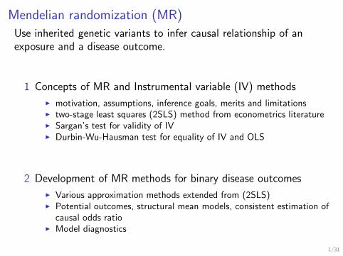
Mendelian randomization (MR)

Use inherited genetic variants to infer causal relationship of anexposure and a disease outcome.

1 Concepts of MR and Instrumental variable (IV) methods

motivation, assumptions, inference goals, merits and limitations two-stage least squares (2SLS) method from econometrics literature Sargan’s test for validity of IV Durbin-Wu-Hausman test for equality of IV and OLS

2 Development of MR methods for binary disease outcomes

Various approximation methods extended from (2SLS) Potential outcomes, structural mean models, consistent estimation of

causal odds ratio Model diagnostics

1/31

Hill’s criteria: when can observed association be

interpreted as causal?

Association 6= Causality

Strength: Lung cancer death rate in smokers about 9-10 times as non-smokers

Consistency: repeatedly observed

Specificity: certain type of disease but not others

Temporality: cause precedes consequence

Biological gradient: dose response, for example, lung cancer risk rises linearly with#cigarettes smoked daily

Biological plausible

Coherent with lab evidence

Experimental or semi-experimental: if exposure was remove, does that prevent thedisease?

Analogy with known exposure-disease causal effect

Hill AB. Proceedings of the Royal Society of Medicine. 1965

2/31

Mendelian randomization analysis

The fundamental idea: If we cannot randomize the exposure, we can finda randomized instrumental variable to disentangle

Confounding

Reverse causation

3/31

Part I

Mendelian randomization: concepts, assumptions, 2SLS, etc

4/31

Katan M. Lancet 1986: a one-page letter

Low cholesterol levels are sometimes associated with increasedcancer risks, but it could be reverse causation.

Differences in the amino acid sequence of apolipoprotein E (apo E)are major determinants of plasma cholesterol levels: E-2, E-3, E-4with increased cholesterol levels.

“if a naturally low cholesterol favours tumour growth, then subjectswith the E-2/E-2 or E-2/E-3 phenotype should have an increasedrisk of cancer.”

Reverse causation“Unlike most other indices of lipid metabolism, apolipoprotein aminoacid sequences are not disturbed by disease, and the apo E phenotypefound in a patient will have been present since birth.”

5/31

The reasoning behind Katan M. Lancet 1986

low cholesterol ⇐⇒ increased cancer risk

1 Apo E sequence variation ⇒ low cholesterol, this relationship isestablished since inheritance of Apo E sequence variation

2 Apo E sequence variation ⇒ increase cancer risk, cancer occurslater stage of life

Two underlying assumptions: Apo E genetic effect on cancer risk can beunbiased assessed; Apo E genetic variation does not increase cancer riskthrough other pathways.

6/31

George Davey Smith and Shah Ebrahim 2003 IJE: first

expanded presentation of MR

Confounding“One key point is that the distribution of such polymorphisms is largelyunrelated to the sorts of confounderssocioeconomic or behaviouralthat wereidentified above as having distorted interpretations of findings fromobservational epidemiological studies.”

Mendel’s second law, the law of independent assortment, germline geneticvariants can be viewed as if “randomized” conditional on parentalgenotypes.

But it is an approximation in the population! 7/31

Conceptual analogy between MR and randomized clinical

trials (RCT)

In RCT, confounding is removed by strict randomization. MR has at best “approximaterandomization”.

In RCT, assignment exerts effect on disease endpoints through actually treatmentreceived. MR has to assume that there is no direct effect from gene to disease (noother pathway).

Nitsch et al. Am J Epidemiol 20068/31

The objectives of MR studies

Analytical goals with proper assumptions

Testing causal relationship between intermediate phenotype anddisease outcome, by testing association between genotypicinstrument and disease outcome: hypothesis testing - the Katan’soriginal reasoning

In linear and sometimes logistic models, estimating causal effect ofintermediate on disease outcome: effect estimation after connectingto instrumental variables approach in econ

9/31

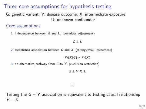
Three core assumptions for hypothesis testing

G: genetic variant; Y: disease outcome; X: intermediate exposure;U: unknown confounder

Core assumptions

1 independence between G and U, (covariate adjustment)

G ⊥ U

2 established association between G and X , (strong/weak instrument)

Pr(X |G) 6= Pr(X )

3 no alternative pathway from G to Y , (exclusion restriction)

G ⊥ Y |X ,U

⇓

Testing the G − Y association is equivalent to testing causal relationshipY − X .

10/31

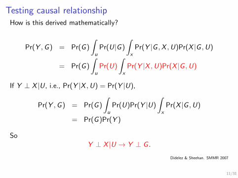
Testing causal relationshipHow is this derived mathematically?

Pr(Y ,G ) = Pr(G )

∫

u

Pr(U|G )

∫

x

Pr(Y |G ,X ,U)Pr(X |G ,U)

= Pr(G )

∫

u

Pr(U)

∫

x

Pr(Y |X ,U)Pr(X |G ,U)

If Y ⊥ X |U, i.e., Pr(Y |X ,U) = Pr(Y |U),

Pr(Y ,G ) = Pr(G )

∫

u

Pr(U)Pr(Y |U)

∫

x

Pr(X |G ,U)

= Pr(G )Pr(Y )

SoY ⊥ X |U → Y ⊥ G .

Didelez & Sheehan. SMMR 2007

11/31

Estimating causal effect in linear models

Two more assumptions required for estimation:

the effect of X on Y is linear,

no interaction between X and U,

Suppose the data generating models are

X = α0 + α1G + α2U + ε1,

Y = θ0 + θ1X + θ2U + ε2.

we can fit the following reduced models

E [X |G ] = α0 + α1G ,

E [Y |G ] = β0 + β1G ,

12/31

IV estimators are essentially ratio estimators

Observe that

β1 = E [Y |G = g + 1]− E [Y |G = g ]

= θ1(E [X |g + 1]− E [X |g ]) + θ2(E [U|g + 1]− E [U|g ])= θ1α1.

Therefore θ1 = β1/α1.

When there is one causal effect, one instrument, the IV estimatorcan be written as the ratio of two OLS estimator

βIV =β1α1

The variance of α1 is important; highly variable in small samples!

Didelez & Sheehan. SMMR 2007;16:309−330

13/31

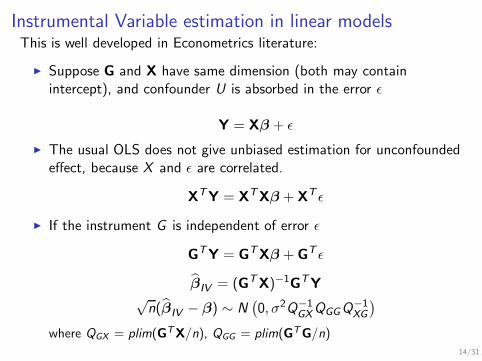
Instrumental Variable estimation in linear modelsThis is well developed in Econometrics literature:

Suppose G and X have same dimension (both may containintercept), and confounder U is absorbed in the error ǫ

Y = Xβ + ǫ

The usual OLS does not give unbiased estimation for unconfoundedeffect, because X and ǫ are correlated.

XTY = X

TXβ + X

T ǫ

If the instrument G is independent of error ǫ

GTY = G

TXβ + G

T ǫ

βIV = (GTX)−1

GTY

√n(βIV − β) ∼ N

(0, σ2Q−1

GXQGGQ−1XG

)

where QGX = plim(GTX/n), QGG = plim(GTG/n)

14/31

This is the same as the ratio estimator in the simple case

Suppose X = (1,X ), G = (1, g)

βIV = (GTX)−1

GTY

= (GTX)−1(GT

G)(GTG)−1

GTY

= (GTG)−1(GT

X)−1(GTG)−1

GTY

It can be verified that

βIV =β1α1

where β1 is the slope of regressing Y on g , α1 is the slope of regressingX on g .

15/31

Generalized methods of momentWhat if G has more dimension (l) than X (p)? More equations than thenumber of parameters.....

gn(β) =1

nG

T (Y − Xβ)

If l == p, setting gn(β) = 0 gives methods of moment estimator.

More generally, for some l × l matrix Wn >0, let

Jn(β) = ngn(β)TWngn(β)

the goal is to set Jn(β) ”close” to zero

βGMM = argminJn(β)

= (XTG)Wn(G

TX)−1(XT

G)Wn(GTY)

The scale of Wn does not change βGMM

16/31

What is the optimal Wn?

Suppose √ngn(β) →d N (0,Ω)

where Ω = E (GTi Giσ

2).

Suppose Wn →p W0, 1/nXTG →p Q, The asymptotic distribution

√n(βGMM − β) →d N (0,Vβ)

where Vβ = (QTW0Q)−1(QTW0ΩW0Q)(QTW0Q)−1)

In IID cases, the optimal Wn →p W0 = Ω−1. Wn = ( 1nGTGσ2)−1,

and so the optimal estimator is

(XTG)(GT

G)−1(GTX)−1(XT

G)(GTG)−1(GT

Y)

17/31

Two-stage least squares (2SLS) estimator

βIV =(X

TG(GT

G)−1G

TX

)−1 (X

TG(GT

G)−1GTY

),

√n(βIV − β) ∼ N

(0, σ2(QGXQ

−1GGQXG )

−1)

This is a 2SLS estimator, computationally simple and stable, firstcompute X

X = G(GTG)−1

GTX

then regress Y on X

βIV = (XTX)−1

XTY

= [XTG(GT

G)−1G

TX]−1

XTG(GT

G)−1G

TY

any regression software can be used to get 2SLS estimator, justcompute the variance

18/31

The fundamental idea observed from 2SLS

Use instrumental variables to extract that variation in intermediatephenotype (exposure) that is independent of confounding variables, anduse this part of variation to estimate the causal effect

The assumptions except the correlation between X and G are notdirectly testable, because of the presence of unmeasuredconfounding U.

There is less appreciation in evaluating and testing theseassumptions

The binary disease outcomes are difficult to work with the conceptof IV (Lecture 2).

19/31

Caution about assumptions

1 Randomization is approximation at best (untestable)

Deviation from “a natural RCT” can be introduced by populationstratification, unknown demographic/behavioural/confounders.....

2 Known association between G and X (testable, but geneticassociations are weak)

Weak genetic instrument and so poor estimation of causal effect, lowpower

3 No other pathway from G to Y other than through X (exclusionrestriction, untestable)

Pleiotropy, linkage disequalibrium with other variants that are alsorelated to Y

20/31

Relaxed assumptions: adjust for known confounders

Suppose there is a set of known confounders W (populationstratification, demographic/behavioral/socioeconomical factor), denoteU to be unknown confounders.

1 G ⊥ U|W2 G correlate with X |W3 G ⊥ Y |X ,U,W

Testing Y ⊥ X |W ,U is equivalent to testing Y ⊥ G |W .

In linear models, θ1 = β1/α1 still holds

E [Y |X ,W ,U] = θ1X + θ2W + θ3U

E [X |G ,W ] = α1G + α2W

E [Y |G ,W ] = β1G + β2W

all the previous math works!

21/31

Overidentifying restrictions and Sargan’s test

We can detect pleiotropy and the validity of IV if

The number of IVs (l) is more than the number of causal effects (p)to be estimated; not all l equations can be exactly zero

The null hypothesis is G ⊥ (Y − Xβ) instrument is orthogonal to the error term there is no direct effect left once conditional on X

Sargan’s test for 2SLS for l instrumental variables and 1 causaleffect

G(Y − θ2SLSX)T σ2(G)TG)−1G(Y − θ2SLSX) → χ2(l − 1)

under the null that all instruments are valid.

Sargan (1958); Small (2007) JASA

22/31

J-statistic

Hansen (1982) gave general results

Jn(β) = ngn(β)TWngn(β) → χ2(l − p)

as long as Wn converges to the optimal W0 and β is efficient GMMestimator

Large J-statistic will reject null hypothesis so that at least oneinstrument might be invalid.

report this J-statistic whenever there are overidentifying conditionsfor IV.

Hansen (1982)

23/31

Test the equality of IV estimator and OLS estimator

The null hypothesis is OLS is consistent and fully efficient

If there is no unmeasured confounding, OLS estimator will beconsistent and efficient; IV is consistent under null or alternative

Large discrepancy between βOLS and βIV suggests that there isconfounding and OLS can not be trusted.

Durbin-Wu-Hausman test

(βIV − βOLS)TD−1(βIV − βOLS ) →d χ2(p)

where D = Var(βIV )− Var(βOLS)

The derivation of the variance comes from the zero correlationbetween βOLS and βIV − βOLS under the null.

Hausman 1978 Econometrika

24/31

Examples of MR

From Jan 2003 to Dec 2013, 179 MR studies were found in PubMed, Medline,Embase and Web of Science (Boef et al (2015) IJE).

PCSK9 genetic variation related to low LDL cholesterol and decreasecoronary heart disease

MR analysis suggests causality in Cohen et al 2006 NEJM;354:1264-72

Two large RCTs confirmed in 2015 (Sabatine et al NEJM;Robinson et al NEJM)

Observational studies suggest Lp-PLA2 levels predict CHD

MR analysis against causality (Wang et al 2010 Thrombosis Research) Subsequent large RCTs failed to find the benefit (STABILITY investigators

NEJM 2014;Nicholls et al 2014 JAMA)

CRP did not show causal effect on a number of cardiometabolic outcomes;therapies toward CRP are discouraged.

More examples can be found in Davey Smith 2015 doi: http://dx.doi.org/10.1101/021386.

25/31

A MR example

Circulating CRP levels are associated with a range of metabolic andcardiovascular diseases (all continuous outcomes in the paper), but notnecessarily causal

CRP haplotype (most likely ones) was used as instrumentalvariables (likely no other pathway other than circulating CRP)

CRP haplotype is not associated with potential confoundingvariables, such as smoking, alcohol, physical activity etc

26/31

A MR example

Strong association between CRP haplotypes and plasma CRP(F-statistic >10), it is not weak instrument

It would be nice to perform a Sargan’s test for validity ofinstruments.

27/31

Difference between MR and observed association

IV estimators are computed by 2SLS

Durbin-Wu-Hausman test for equality of IV and OLS

These results suggest that there is no causal association betweenCRP and the metabolic syndrome phenotypes.

28/31

Scientific merit of MR studies

Smith & Ebrahim 2003 IJE:

Concluding remark

“For the present, however, it is probably fair to say that the methodoffers a more robust approach to understanding the effect of somemodifiable exposures on health outcomes than does much conventionalobservational epidemiology. Where possible randomized controlled trialsremain the final arbiter of the effects of interventions intended toinfluence health, however.”

29/31

Softwares for IV analysis

Stata has extensive commands for IV regression: ivregress,ivreg2 implementing 2SLS, Sargan’s test or J-statistic,Durbin-Wu-Hausman test

R package AER has ivreg function; very powerful gmm package

30/31

Reference Hill AB. The environment and disease: association and causation? Proceedings of the

Royal Society of Medicine. 1965;58:295-300 Katan M. Apolipoprotein E isoforms, serum cholesterol, and cancer.

Lancet.1986;327:507-508. Davey Smith G, Ebrahim S. Mendelian randomization: can genetic epidemiology

contribute to understanding environmental determinants of disease. International

Journal of Epidemiology. 2003;32:1-22. Didelez V, Sheehan NA. Mendelian randomisation as an instrumental variable approach

to causal inference. Statistical Methods in Medical Research. 2007;16:309-330. Davidson R, MacKinnon J. Estimation and Inference in Econometrics. 1993. Oxford

University Press, New York. Didelez V, Meng S, Sheehan, NA. Assumptions of iv methods for observational

epidemiology. Statistical Science. 2010;25:22-40. Hernan MA, Robins JM. Instruments for causal inference: an epidemiologists dream?

Epidemiology 2006; 17:360372. Hansen, L. 1982. Large sample properties of generalized method of moments

estimators. Econometrica 50(3): 1029-1054. Sargan, J. 1958. The estimation of economic relationships using instrumental variables.

Econometrica 26(3): 393-415. Hausman, J. 1978. Specification tests in econometrics. Econometrica 46(3):

1251-1271. Small DS. Sensitivity analysis for instrumental variables regression with overidentifying

restriction. JASA 2007;102:1049-1058.

31/31