UNIVERSITY OF LJUBLJANAFaculty of mathematics and physics

Laser Doppler vibrometry and modal testing

author: Rok Prislan

mentor: dr. Daniel Sven²ek

Abstract

This paper introduces laser Doppler vibrometry as a modern technique for measuring objectsdynamics. It explains all the needed physical and data processing background which brings tothe velocity and displacement information. The dynamic parameters of the object are given bymodal testing, which is presented in addition.

Ljubljana, 1. April 2008

Contents

1 Introduction 3

2 Laser Doppler vibrometry 4

2.1 Laser . . . . . . . . . . . . . . . . . . . . . . . . . . . . . . . . . . . . . . . . . . . . 42.2 Doppler e�ect . . . . . . . . . . . . . . . . . . . . . . . . . . . . . . . . . . . . . . . 42.3 Vibrometer . . . . . . . . . . . . . . . . . . . . . . . . . . . . . . . . . . . . . . . . 5

2.3.1 Heterodyne interferometer . . . . . . . . . . . . . . . . . . . . . . . . . . . . 62.3.2 Homodyne interferometer . . . . . . . . . . . . . . . . . . . . . . . . . . . . 72.3.3 Measuring objects with multiple degrees of freedom . . . . . . . . . . . . . . 8

2.4 Signal processing . . . . . . . . . . . . . . . . . . . . . . . . . . . . . . . . . . . . . 82.4.1 Velocity estimation . . . . . . . . . . . . . . . . . . . . . . . . . . . . . . . . 92.4.2 Displacement estimation . . . . . . . . . . . . . . . . . . . . . . . . . . . . . 9

2.5 Scanning vibrometer . . . . . . . . . . . . . . . . . . . . . . . . . . . . . . . . . . . 92.6 Surface properties . . . . . . . . . . . . . . . . . . . . . . . . . . . . . . . . . . . . . 10

3 Modal testing 11

3.1 Measurement . . . . . . . . . . . . . . . . . . . . . . . . . . . . . . . . . . . . . . . 113.2 Parameters estimation . . . . . . . . . . . . . . . . . . . . . . . . . . . . . . . . . . 13

4 Conclusion 15

5 Appendix: Acousto-optic modulator 16

2

Chapter 1

Introduction

Laser Doppler vibrometry (LDV) is a velocity and displacement measurement technique. Itstheoretical bases were only presented in the second half of the 20th century in spite having hadall the needed physical knowledge for a long time. LDVs relatively late development is related tothe late laser development which is its basic component (the �rst working laser was demonstratedin 1960). The use of LDV is nowadays spread in a variety of �elds. It is used for the analysis ofall kinds of vibrating systems, speed and position measurement. A typical modern vibrometer iscomposed of the a sensor head unit and a controller unit (1.1).

The LDV measurement is non-contact

Figure 1.1: An exampel of a modern vibrometerfrom Polytec. Composed of a sensor head and acontroller (processing unit) [2].

and that is its biggest advantage. Thereforethe tested part stays unin�uenced during themeasurement bringing a much more reliablepicture of its own properties. Because of thisit is possible to observe dynamics on a verybroad scale down to micron size. Alterna-tives to the LDV are acceleometers whichsupply a better sensitivity and are less sensi-tive to vibrations of the enviroment becausethey are not part of it. On the other handthis is a contact method that in�ueces themeasurment object with its own mass. An-other disadvadage of the acceleometers areproblems with �xation which also makes thechange of the observation point complicated [1].

The basic component of a LDV aperture is a laser beam focused on the tested structure which'smovement causes the presence of the Doppler e�ect in the laser re�ection. If the object suppliesa proper re�ection, it is possible to calculate its displacement and velocity. How exactly this isdone will be explained in the second chapter while modal testing will be presented in the thirdchapter.

3

Chapter 2

Laser Doppler vibrometry

Before entering into the in-deep explanation of LDV the understanding of its basic component isneeded. Therefore the properties of the laser and the Doppler e�ect should be discussed.

2.1 Laser

The word "LASER" is an acronym (Light

Figure 2.1: Laser structure [4].

Ampli�cation by Stimulated Emission ofRadiation) which also explains how it works.The basic principle is the principle of theinduced emission of photons. The laserconsists of a resonant optical cavity whichcontains the lasing material (gain medium)which supplied with energy places some ofits particles into excited quantum states.The pumping of energy is usually donewith electrical current, light �ashes or evenwith lasers. The excited particles releasethe additional energy by emitting photons(2.1) spontaneously or stimulated by otherphotons with proper energy. The cavity has therefore mirrors on each end that are repeatedlyre�ecting light. The length of the cavity de�nes the wavelength of the re�ecting light and mustbe tuned to the di�erence of quantum energy levels of the gain medium. If so, the light in thecavity is ampli�ed. In addition one of the re�ecting mirrors is partially transparent letting someof the light out of the cavity in the form of a beam [3].

The cavity dimensions do not only well de�ne the emitted light wavelength (monochromatic),but the cavities bounds make the laser a coherent light source (re�ection boundary condition).Why a monochromatic and coherent light source is needed will be explained later, but that areexactly the properties of a laser. The lasers used for LDV are usually helium-neon with thewavelength 0.6328 µm (the following text will refer to it on many occasions).

2.2 Doppler e�ect

This physical phenomena was �rstly observed by the Austrian physicist Christian Doppler. Itdescribes the relative change in wavelength and frequency of a wave when the observer and thesource are moving. The waves can be grouped according to the medium/non-medium propagationand in both cases the Doppler e�ect can be observed (2.2). But when talking about wavespropagating in medium relative velocities of the source and of the observer comparing the mediummust be taken into account. On the other hand only the relative di�erence in velocity betweenthe observer and the source is important for the electromagnetic waves.

4

Figure 2.2: Examples of Doppler e�ect. Left picture: a stationary microphone records movingpolice sirens at di�erent pitches depending on their relative direction. Right picture: a redshiftof spectral lines in the optical spectrum of a supercluster of distant galaxies (lower), as comparedto that of the Sun (upper) [6] .

LDV uses a laser which is an electromagnetic wave. The light source is �xed and the observa-tion object is moving. The object would measure a di�erent frequency (f ′) as it is emitted

f ′ = f

(c

c± v

).

f stands for the emitted wave frequency, c (299792458 m/s) for its propagation velocity and v forthe velocity of the object. The ± sign in the denominator depends on the way the observed objectis moving. If it moves away from the source the plus sign should be taken and the frequency isbeing lowered. It is the way around for moving toward the source.

Light speed is very big compared to the speed of the observed object. Therefore the equationcan be evolved in a Taylor series

f ′ = f

(c

c± v

)≈ f

(c∓ vc

)= f

(1∓ v

c

)= f + fd (2.1)

The frequency shift is denoted with fd = f vc (Doppler frequency). Equation (2.1) expresses thefrequency the moving object would measure, but in the LDVs case the re�ected light is observed.Therefore the Doppler e�ect must be taken into account again. Now the source is moving andthe observer is �xed and the overall frequency shift doubles

fd = 2fv

c= 2

v

λ

where λ is the wavelength of the laser.

2.3 Vibrometer

At this point all the needed physical background is explained and the explanation of LDV ispossible [2]. Measuring the frequency of the re�ected laser would give the velocity of the object.Unfortunately the laser has a very high frequency (ω = 4.74 · 1014Hz for the he-ne laser) anda direct demodulation is not possible. The solution is to observe the interference between there�ected and the original light. An optical interferometer is therefore used to mix the scatteredlight coherently with the reference beam. The photo detector measures the intensity of the mixedlight of which the beat frequency is equal to the di�erence frequency between the reference andthe measurement beam. Such an arrangement can be a Michelson interferometer (2.3).

A laser beam is divided at a beam splitter into a measurement beam and a reference beamwhich propagates in the arms of the interferometer. The distances the light travels between thebeam splitter and each re�ector are xr for the reference beam and xm for the measured object. The

5

Figure 2.3: The micholson interferometer is the basic set up for the LDV.

corresponding optical phases of the beams in the interferometer are ϕr = 2kxr and ϕ(t)m = 2kxm,where k = 2π/λ. In LDVs case only the re�ected phase is time dependent while the referencephase is �xed because the distances are not changing. The phase di�erence between the mixedbeams is introduced ϕ(t) = ϕr − ϕm = 2k∆L, where ∆L is the vibrational displacement of theobject and λ the wavelength of the laser light.

Mathematically both beams can be treated as free waves.

Er = Er0eı(ωrt+ϕr)

Em = Em0eı(ωmt+ϕm) = Em0e

ı((ωr+ωd)t+ϕr−ϕ(t)) = Em0eı(ωrt+ϕr)eı(ωdt−ϕ(t)).

The photo detector measures the time dependent intensity I(t) at the point where the measurementand reference beams interfere.

I(t) = |Em + Er|2 = Im + Ir + 2√ImIr cos (ωd(t)t− ϕ(t))

Introducing K is a mixing e�ciency coe�cient and R is the e�ective re�ectivity of the surface theintensity equation becomes

I(t) = ImIrR+ 2K√ImIrR cos (ωdt− ϕ(t)).

If ∆L changes continuously the light intensity I(t) varies in a periodic manner. A phase change ϕof 2π corresponds to a displacement ∆L of λ/2. Now it is obvious why for LDV a laser is needed.Having a monochromatic and coherent light source is important for having a well de�ned phaseand wavelength.

From the phase of the intensity it is possible to calculate the displacement. But getting thephase information is not that easy. As object movement away from the interferometer generatesthe same interference pattern as object movement towards the interferometer, this setup cannotdetermine the direction the object is moving in. By changing the measurement setup, thereare two ways to introduce directional sensitivity (Homodyne and Heterodyne). In the next twosections both of them are explained.

2.3.1 Heterodyne interferometer

An acousto-optic modulator (called also Bragg cell, see Appendix: Acousto-optic modulator) isplaced in the reference beam (2.4), which statically shifts the light frequency by tipicaly fb = 40MHz. By comparison, the frequency of the laser light is 4.74 ·1014 Hz. The frequency shift causesa modulation frequency of the fringe pattern of 40 MHz when the object is at rest. This waythe objects zero velocity position is transposed and directional sensibility is introduced. If theobject moves towards the interferometer, the modulation frequency is reduced and if it movesaway the frequency is raised. This means that it is now possible not only to detect the amplitudeof movement but also to clearly de�ne its direction.

6

Figure 2.4: A heterodyne interferometer. The additional Bragg-cell produces a frequency shift inthe reference laser beam.

A mathematical formulation of a heterodyne interferometer can be done. The reference fre-quency (f) changes and therefore the frequency di�erence changes

∆f = f − f ′ = −fd −→ ∆f = f + fb − f − fd = fb − fd

and the intensity at the detector becomes

I(t) = ImIrR+ 2K√ImIrR cos(2π[fb − fd]t− ϕ(t)) (2.2)

Now the cos part of the intensity never varies with negative frequencies and threfore directionalsensibility is introduced.

2.3.2 Homodyne interferometer

The second solution known as the quadrature homodyne interferometer can be designed by addingwave retardation plates, a polarizing beamsplitter and an additional detector [2]. The interferom-eter polarizes the laser to a 45◦ inclination. The light in the reference arm passes twice throughthe λ/8 retardation plate and the light coming back to the beam splitter is circularly polarized.This can be described as the vector sum of two orthogonal polarization states (2.5).

Figure 2.5: A homodyne interferometer. The additional polarizer, λ/8 plate, a beam splitter anda photo detector are inserted into the measuring system.

A polarizing beamsplitter placed in front of the detectors 1 and 2 separates the two orthogonalcomponents. The result is a quadrature relationship at the detectors (sine and cosine output).Out of the interference patterns of the re�ected signal with both signal components the direction of

7

the movement can be calculated. Between the sine and cosine component is a 90◦ phase di�erenceand therefore di�erent movement directions cause a di�erent interference pattern at least withone of the reference component.

A quadrature homodyne interferometer is much easier to design as simple low frequency photodetectors and ampli�ers can be used, but non-linear behavior of the used elements on the otherhand causes harmonic distortions of the measurement signal. Because of this Homodyne interfer-ometers are usually used for LDVs.

2.3.3 Measuring objects with multiple degrees of freedom

Introducing the directional sensibility it is now possible to detect the movement parallel to the laserbeam. In the case the movement is not only in the beam direction only the parallel componentis measured. It is possible to measure motion in more direction using multiple LDVs in di�erentsetups 2.6.

Figure 2.6: Di�erent measuring setups allow to analyse more complex movements using multipleLDVs [2].

2.4 Signal processing

In the Homodyne case the interference frequency is proportional to the surface velocity and thephase change ∆ϕ is proportional to the displacement of the object. Typical performances of amodern LDV are presented in the lower table. How the the displacement and velocity is calculationout of the measured intensity must be explained.

8

from to

Frequency 0 30 MHz

Vibration Amplitudes 2 pm 10 m

Vibration Velocities 50 nm/s 30 m/s

2.4.1 Velocity estimation

Typical frequencies that should be analysed are moving between 30 MHz and 50 MHz. That isin the RF range, which is de�ned between 3 Hz and 300 GHz.

The analogue way to do the decoding is to use a PLL (phase locked loop). PLL is a controlsystem that generates a signal that has a �xed relation to the phase of a "reference" signal. InLDV's case the interference intensity signal is used for the "reference". The phase-locked loopcircuit responds to the frequency and to the phase of the input signals, automatically raisingor lowering the frequency of a controlled oscillator until it is matched to the reference in bothfrequency and phase. From the voltage on the oscilator the frequency is read.

Digital demodulation is another way to measure the frequency. Firstly the signal must bedigitalised with an AD converter. For this purpose high speed converters should be used becausehigh frequencies are present. Out of the data stream the velocity information is taken with theuse of numerical methods (convolution, FFT).

2.4.2 Displacement estimation

To measure displacement the fringe counting technique is used. As displacement by half the laserwavelength (λ/2 = 316nm for He-Ne lasers) changes the phase by 360 degrees. By counting the"zero-crossings" the laser vibrometer measures how far the object has moved, in increments of λ2per cycle. The information about the direction of the movement should be taken from the velocityinformation.

In the case of digital LDVs the data is interpolated. Doing so the determination of "zero-points" is done with a better resolution that leads to a better accuracy of the dipslacementmeasuremen. Another way to increase the resolution is to arange multiple re�ections from theobject. In that case bigger frequency shifts and phase changes are detected for the same movement.This way resolutions of λ/160 (2 nm for He-Ne laser) are achieved. It should be noted that, thehigher the phase multiplication becomes the lower the measurable velocity and vibration frequencyof the object will be.

2.5 Scanning vibrometer

Scanning vibrometers use a single point vibrometer (discussed until now) for analysing biggerareas of an object. The measurement system is equipped with an additional video camera whichis connected to the control unit. Through a computer based user interface the scanning area isselected with the help of smart picture recognition algorithm (2.7).

The sensor head of the vibrometer is equipped with a moving mirrors mechanism driven bythe control unit that scan the selected area in discrete points. Each point is being measured fora certain time period which de�nes the precision of the frequency estimation. Simultaneouslythe displacement and the velocity is measured and stored in the computer memory. After themeasurement the data can be presented graphically making a very good picture of an object'sdynamics. With scanning vibrometers amazing pictures are produced with all the precision thatthe LDV technique is o�ering (2.8).

When using scanning vibrometers a basic assumption is made: the vibrating object is vibratingin the same way all during the measurement. This is the assumption of stationary vibration.

9

Figure 2.7: Through a computer based interface it is possible to estimate the scanning area. Thepicture shows the interactive grid which de�nes the measurement points on a cars mudguard [2].

Figure 2.8: Scanning LDVs are broadly used in di�erent industrial �elds. Amazing surface scansgive very clear pictures of the properties of an object [2].

2.6 Surface properties

LDVs operate on a variety of surfaces [2]. It is important that the amount of light scatteredback from the di�erent surfaces is su�cient for further signal analysis. Specular surfaces obeythe law: angle of incidence is equal to the angle of re�ection. When making measurements fromsuch surfaces the optics of the LDV need to be aligned such that the re�ected light returns withinthe aperture of the collecting optics (2.9). Di�use surfaces scatter the incident light over a largeangular area. In this case bigger measuring angles are possible if there is a satisfying intensity ofthe re�ected light.

It is possible to increase the re�ection of the surface in the lasers beam direction using retro-re�ective tape or paint. This material consists of small glass spheres (approximately 50 µ m indiameter) that are glued with an elastic epoxy to the base material. Each sphere acts as a small"cats eye" scattering light back along the path of the incident beam.

10

Chapter 3

Modal testing

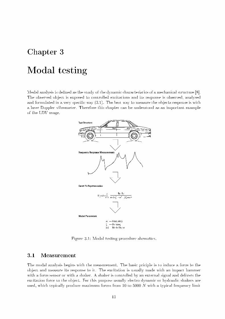
Modal analysis is de�ned as the study of the dynamic characteristics of a mechanical structure [8].The observed object is exposed to controlled excitations and its response is observed, analysedand formulated in a very speci�c way (3.1). The best way to measure the objects response is witha laser Doppler vibrometer. Therefore this chapter can be understood as an important exampleof the LDV usage.

Figure 3.1: Modal testing procedure shematics.

3.1 Measurement

The modal analysis begins with the measurement. The basic priciple is to induce a force to theobject and measure its response to it. The excitation is usually made with an impact hammerwith a force sensor or with a shaker. A shaker is controlled by an external signal and delivers theexcitation force to the object. For this purpose usually electro-dynamic or hydraulic shakers areused, which typically produce maximum forces from 10 to 5000 N with a typical frequency limit

11

between 5 and 20 kHz. A shaker can deliver sinus sweep and random noise excitations while ahammer produces impact excitations.

The data of interest is the response (displace-

Figure 2.9: A highly re�ect-ing surface. The observedsurface must be nearly per-pendicular to the laser beam.

Figure 3.2: Piezoelectric material generatean electric potential in response to appliedmechanical stress.

ment, velocity, acceleration) and the excitation force.The response data is delivered by a LDV or ac-celerometer which were allready discussed. On theother hand the excitation force information comesfrom a force transducer. The piezoelectric typesof transducers, which measure force and accelera-tion, are the most widely used for modal testing.Piezoelectricity is the ability of some materials (no-tably crystals and certain ceramics) to generate anelectric potential in response to applied mechanicalstress (3.2). The word is derived from the Greekpiezein, which means to squeeze or press. A gen-eral test con�guration is presented on Figure 3.3.

Figure 3.3: General test con�guration including all the main parts [8].

The �rst step in setting up a structure for frequency response measurements is to consider the�xturing mechanism necessary to obtain the desired constraints (boundary conditions). This isa key step in the process as it a�ects the overall structural characteristics. Analytically, bound-ary conditions can be speci�ed in a completely free or completely constrained sense. In testingpractice, however, it is generally not possible to fully achieve these conditions. The free conditionmeans that the structure is �oating in space with no attachments to ground and exhibits rigidbody behavior at zero frequency. Physically, this is not realizable, so the structure must be up-ported in some manner. The constrained condition implies that the motion is set to zero, whichis also impossible to achieve.

In order to approximate the free system, the structure can be suspended from very soft elasticcords or placed on a very soft cushion. By doing this, the structure will be constrained to adegree and the rigid body modes will no longer have zero frequency. However, if a su�ciently softsupport system is used, the rigid body frequencies will be much lower than the frequencies of the�exible modes and thus have negligible e�ect.

The implementation of a constrained system is much more di�cult to achieve in a test envi-ronment. To begin with, the base to which the structure is attached will tend to have some motionof its own. Therefore, it is not going to be purely grounded. Also, the attachment points will have

12

some degree of �exibility due to the bolted, riveted or welded connections. One possible remedyfor these problems is to measure the frequency response of the base at the attachment points overthe frequency range of interest. Next thing is to verify that this response is signi�cantly lowerthan the corresponding response of the structure, in which case it will have a negligible e�ect.

Finally the measurement can start. The hole process is managed by the controller which setsthe input excitation and measures the output response simultaneously according to the will of theuser. The excitation signal is connected to an ampli�er which assures enough power for the shaker.The force and the response is aquired during the experiment and afterwards objects parametersare estimated out of it.

3.2 Parameters estimation

Knowing the excitation force and the re-

Figure 3.4: Block diagram of the measurement.G(s) is describing the object's dynamics.

sponse of the object, it's dynamic propertiescan be estimated (3.4). Finding it's trans-fer function brings the value of the system'sdamping factors, moving mass and sti�nessparameters. The transfer function of a sys-tem is de�ned as the Laplace transformationof the ratio of the input and output signal

G(s) =Y (s)X(s)

=L{y(t)}L{x(t)}

.

All real systems of �nite extent have an in�nite number of possible vibration modes [10].Suppose that the equation describing wavelike propagation in the oscillator has the form

LΦ− ∂2Φ∂t2

= 0 (3.1)

where L is a linear di�erential operator. The equation can be written in form of eigenfunctions

LΦj + ω2jΦn = 0.

Extending equation 3.1 by adding a a force unit magnitude on right at frequency ω appliedat point r0 this equation becomes

LHω + ω2Hω = −δ(r− r0) (3.2)

where δ(r− r0) is the Dirac delta function and Φ → Hω(r, r0), which is the Green function forthe system at the frequency ω. Assuming the expansion

Hω(r, r0) =n∑j

anΦj(r)

and substituting this into 3.2

n∑j

aj(ω2j − ω2)Φj(r) = δ(r− r0) (3.3)

it is possible to express aj by multiplying both sides of 3.3 with Φj(r) and integrating over thehole volume of the resonator using the ortonormality condition. Now it is possible to express theGreen function

Hω(r, r0) =n∑j

Φj(r0)Φj(r)ω2j − ω2

(3.4)

13

This is the equation on picture 3.1 and is expressing the transfer function dependence of themeaurement and excitation point. If both points are chosen to be the same the "driving transferfunction" is measured, otherwise we talk about "cross transfer function.

The transfer function must �t the measured data in the form of a rational function whichhas a well understandable physical background. By �tting the response with a rational functionthe linearity assumption is made. On one hand linearity is limiting to harmonic solutions whichare nothing else than a supposition and no shocking results can be achieved. But luckily thisassumption is easy to verify. A linear system can respond only by the frequency it was excitedwith and only phase and amplitude changes can occur. If this is not true the linearity assumptionis inappropriate.

Modal testing can help making improvements on vibrating systems. If one mode of the systemvibration is in our interest its natural frequency, its dummping factor and sti�ness coe�cientscan be calculated. That means knowing the objects dynamic properties in the form of a di�er-ential equation (3.5). That gives the opportunity to make corrections to the system based onunderstanding and knowledge.

mx+ cx+ kx = f(t) (3.5)

ωn =k

m, 2ζωn =

c

m

14

Chapter 4

Conclusion

LDV is a very sophisticated measurement technique becoming a standard for measuring dis-placements and velocities. Its main advantages are the non contact nature, its wide frequencymeasurement capability, a very high precision, the ability to measure distant objects and its sim-plicity to change the measurement point. All the advantages make it indispensable for analysisin many di�erent �elds. Its commercial success makes it even more a�ordable and broadly used.

The example of modal testing usage was made which gave a close look at the dynamics. Theparameters can be understood and changes to the object can be made easily. Resonances can bemoved from the operating regime and other vibration-connected corrections can be made. Becauseof its high practical value, modal testing is broadly used in many industry �elds.

15

Chapter 5

Appendix: Acousto-optic modulator

An acousto-optic modulator, also called a Bragg

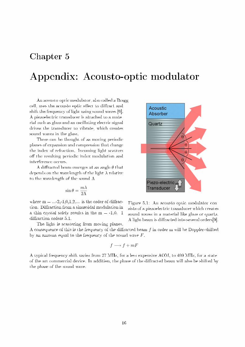
Figure 5.1: An acousto-optic modulator con-sists of a piezoelectric transducer which createssound waves in a material like glass or quartz.A light beam is di�racted into several orders[9].

cell, uses the acousto-optic e�ect to di�ract andshift the frequency of light using sound waves [9].A piezoelectric transducer is attached to a mate-rial such as glass and an oscillating electric signaldrives the transducer to vibrate, which createssound waves in the glass.

These can be thought of as moving periodicplanes of expansion and compression that changethe index of refraction. Incoming light scatterso� the resulting periodic index modulation andinterference occurs.

A di�racted beam emerges at an angle θ thatdepends on the wavelength of the light λ relativeto the wavelength of the sound Λ

sin θ =mλ

2Λ

where m = ...-2,-1,0,1,2,... is the order of di�rac-tion. Di�raction from a sinusoidal modulation ina thin crystal solely results in the m = -1,0,+1di�raction orders 5.1.

The light is scattering from moving planes.A consequence of this is the frequency of the di�racted beam f in order m will be Doppler-shiftedby an amount equal to the frequency of the sound wave F .

f −→ f +mF

A typical frequency shift varies from 27 MHz, for a less-expensive AOM, to 400 MHz, for a state-of-the-art commercial device. In addition, the phase of the di�racted beam will also be shifted bythe phase of the sound wave.

16

Bibliography

[1] http://en.wikipedia.org/wiki/Accelerometer (1.4.2008)

[2] http://www.polytec.com/eur/158_463.asp#Fundamentals (1.4.2008)

[3] http://en.wikipedia.org/wiki/Laser (1.4.2008)

[4] http://people.seas.harvard.edu/~jones/ap216/lectures/ls_2/ls2_u5/ls2_unit_5.html (1.4.2008)

[5] http://www.cartage.org.lb/en/themes/sciences/Physics/Optics/LaserTutorial/Laseroscillator/Laseroscillator.htm (1.4.2008)

[6] http://en.wikipedia.org/wiki/Doppler_effect (1.4.2008)

[7] http://www.polytec.com/int/158_7779.asp (1.4.2008)

[8] http://cp.literature.agilent.com/litweb/pdf/5954-7957E.pdf (1.4.2008)

[9] http://en.wikipedia.org/wiki/Bragg_Cell (1.4.2008)

[10] Fletcher, N.H. and Rosing, T.T. 1990. The Physics of MusicalInstruments. NewYork:Springer-Verlag

[11] Shabana, A. A. 1995. Theory of Vibration. Chichago: Univerity of Illinois. drugaizdaja

17