meranie asf erickyc h optickyc h pl^och pomocou ... · abstrakt cie lom pr ace je zhodnotit mo...
TRANSCRIPT

Univerzita Palackeho Olomouc
Prırodovedecka fakulta
Katedra optiky
DIPLOMOVA PRACA
Meranie asferickych optickych ploch pomocoustandardnych detektorov vlnoplochy
Vypracovala Bc. Sandra Drusova
Obor Optika a optoelektronika
Veduci prace Mgr. Bohumil Stoklasa
Datum odovzdania 28. aprıl 2014

Palacky University, Olomouc
Faculty of Science
Department of optics
MASTER THESIS
Aspherics optical shop testing with standard wavefrontsensors
Written by Bc. Sandra Drusova
Study program Optics and Optoelectronics
Supervisor Mgr. Bohumil Stoklasa
Date April 28, 2014

The Declaration
I declare I have written this thesis myself under the guidance of my supervisor Mgr. Bohumil
Stoklasa. Further I declare that I have used the litterature I have cited.
Olomouc, April 28, 2014
. . . . . . . . . . . . . . . . . . . . . . . . . . . . . . . . . . .
Bc. Sandra Drusova
Aknowledgements
I would like to thank my supervisor, Mgr. Bohumil Stoklasa, for his patient guidance and feedback to
my work. This thesis would not have been possible without colleagues from Measurement methods
development depatment in MEOPTA who helped me in my supervisor’s absence. I must express my
gratitude to Daniel Vacula, Milan Matela and Josef Hnilo working in Optical engineering department
in MEOPTA, who gave me lectures about optical design. Special thanks goes to Peter Klein and
Marta Strakova for their help when my computer broke down few days before finishing my work.

Abstrakt
Cielom prace je zhodnotit moznosti testovania asferickych sosoviek v spolocnosti MEOPTA - op-
tika, s.r.o. Budu pouzite dve dostupne zariadenia, Shack-Hartmannov senzor a Fizeau interfero-
meter. V praci je navrhnuta metoda testovania rotacne symetrickych asfer bez dodatocnej nulovacej
optiky. Ucinnost a obmedzenia navrhnutej metody su experimetalne overene meranım na Fizeau
interferometri. Pre buduce aplikacie boli taktiez navrhnute jednoduche nulovacie kompenzatory.

Abstract
This thesis describes the possibilities for aspherical lens testing in company Meopta - optika, s.r.o.
The suitability of two available devices Shack-Hartmann sensor and Fizeau interferometer is com-
pared by simulating and testing of real aspheres. Method for testing of rotationally symmetric
aspheres without a null optic is proposed. In order to extract the information about the surface
deformations, shape of detected wavefront is predicted by theoretical calculations. Efficiency and li-
mitations of the method are experimentally checked on Fizeau interferometer. Simple refractive
null compensators were designed for the future measurements.

Contents
1 Introduction 2
2 Testing of Aspherical Wavefronts and Surfaces 4
2.1 Mathematical Representation of Aspherical Surfaces . . . . . . . . . . . . . . . . . . 5
2.1.1 Wavefront Description with Zernike Polynomials . . . . . . . . . . . . . . . . 6
2.2 Methods for Aspherical testing . . . . . . . . . . . . . . . . . . . . . . . . . . . . . . 7
2.2.1 Optical Profilometers . . . . . . . . . . . . . . . . . . . . . . . . . . . . . . . 7
2.2.2 Adapted Wavefront Testing . . . . . . . . . . . . . . . . . . . . . . . . . . . . 8
2.2.3 Multiple Wavelength Interferometry . . . . . . . . . . . . . . . . . . . . . . . 10
2.2.4 Subaperture Stitching Interferometry . . . . . . . . . . . . . . . . . . . . . . . 11
2.2.5 Non-adapted Wavefront Testing . . . . . . . . . . . . . . . . . . . . . . . . . . 12
2.3 Measuring Instruments . . . . . . . . . . . . . . . . . . . . . . . . . . . . . . . . . . . 13
2.3.1 Newton Interferometer . . . . . . . . . . . . . . . . . . . . . . . . . . . . . . . 13
2.3.2 Twyman-Green Interferometer . . . . . . . . . . . . . . . . . . . . . . . . . . 13
2.3.3 Fizeau Interferometer . . . . . . . . . . . . . . . . . . . . . . . . . . . . . . . 14
2.3.4 Shack-Hartmann Sensor . . . . . . . . . . . . . . . . . . . . . . . . . . . . . . 16
2.4 Phase Shifting Interferometry . . . . . . . . . . . . . . . . . . . . . . . . . . . . . . . 18
2.4.1 Phase Unwrapping . . . . . . . . . . . . . . . . . . . . . . . . . . . . . . . . . 20
3 Shack-Hartmann Sensor vs. Phase Shifting Interferometry 23
3.1 Comparison . . . . . . . . . . . . . . . . . . . . . . . . . . . . . . . . . . . . . . . . . 23
3.2 Simulation . . . . . . . . . . . . . . . . . . . . . . . . . . . . . . . . . . . . . . . . . . 25
3.3 Discussion . . . . . . . . . . . . . . . . . . . . . . . . . . . . . . . . . . . . . . . . . . 28
4 Non-null Testing 29
4.1 Measurement Procedure . . . . . . . . . . . . . . . . . . . . . . . . . . . . . . . . . . 30
4.2 Computer Program for Theoretical Simulations . . . . . . . . . . . . . . . . . . . . . 33
4.3 Theoretical Limits of Intellium Interferometer . . . . . . . . . . . . . . . . . . . . . . 36
4.4 Comparison of Unwrapping Algorithms . . . . . . . . . . . . . . . . . . . . . . . . . 38
4.5 Experimental Verification of Nyquist Condition . . . . . . . . . . . . . . . . . . . . . 41
4.6 Non-null Testing Results . . . . . . . . . . . . . . . . . . . . . . . . . . . . . . . . . . 42
4.7 Discussion . . . . . . . . . . . . . . . . . . . . . . . . . . . . . . . . . . . . . . . . . . 49

5 Retrace Error 50
5.1 Experimental Approach . . . . . . . . . . . . . . . . . . . . . . . . . . . . . . . . . . 51
5.2 Theoretical Approach . . . . . . . . . . . . . . . . . . . . . . . . . . . . . . . . . . . 53
5.3 Discussion . . . . . . . . . . . . . . . . . . . . . . . . . . . . . . . . . . . . . . . . . . 57
6 Null Testing 59
6.1 Optical Design and Tolerancing . . . . . . . . . . . . . . . . . . . . . . . . . . . . . . 59
6.2 Null Compensators for Aspheres . . . . . . . . . . . . . . . . . . . . . . . . . . . . . 61
6.3 Optimization Results . . . . . . . . . . . . . . . . . . . . . . . . . . . . . . . . . . . . 62
6.3.1 Reflectivity of Aspherical Surface . . . . . . . . . . . . . . . . . . . . . . . . . 66
6.3.2 Tolerance Analysis . . . . . . . . . . . . . . . . . . . . . . . . . . . . . . . . . 66
6.3.3 Mechanics for Null Component . . . . . . . . . . . . . . . . . . . . . . . . . . 70
7 Conclusion 72
A List of Aspheres Used in MEOPTA 74
B Zernike Frindge Coefficients 76
C LENS 7: Measurement Protocol from Asphericon 77
D LENS 6: Mechanics for Null Compensator 78

Chapter 1
Introduction
This master thesis will focus on describing the possibilities of testing surface quality of aspherical
lenses using technologies available in MEOPTA-optika, s.r.o. Aspherical lenses will be tested using
HASO Shack-Hartmann sensor and ESDI Intellium interferometer. The goal is to identify the limi-
tations of both devices, experimentally and theoretically. Theoretical simulations will be performed
on a sample of eleven aspheres used in MEOPTA products. The efficiency of suggested methods
for aspherical testing will be discussed based on results.
MEOPTA uses aspheres in wide range of products, but still cannot manufacture its own aspher-
ical lenses in Prerov.The aspherical lenses have to be ordered from other manufacturers, therefore it
is important to have a method how to test the surface quality. Aspherical lenses are tested together
with other optical elements of the system. If the system performance does not meet the expec-
tations, usually the problem is caused by an aspherical lens. The unsatisfactory lens is sent back
to the manufacturer for additional testing. Having an accurate, economical and reliable measure-
ment method will certainly become a powerful tool in MEOPTA’s hands. Measuring the aspherical
surfaces is more complicated compared to the spherical surfaces and requires expensive beam sha-
ping optics or special techniques. Such kind of solution is not always necessary, so in this master
thesis, we are trying to determine if available aspheres can be measured using conventional methods.
Chapter 2 gives an overview of current aspherical testing methods, instruments and phase shif-
ting interferometry as an important interferogram analysis method.
Chapter 3 includes a theoretical comparison between Shack-Hartmann sensor and interferometric
phase shifting algorithm for reconstruction of an aspherical wavefront. In the simulation, wavefront
is directly imaged on high resolution CCD chip and sampled by microlenses at the same time. The
limitations of both wavefront detection techniques are found.
In the next chapter, Non-null Testing, a procedure for aspherical testing using Intellium interferome-
ter is described in detail. The limits of algorithms reconstructing the wavefront from interferograms
are checked, performance of all available algorithms is compared. Section 4.2 includes the descrip-
tion of program performing the theoretical simulations.
2

The error introduced by interferometer optics is further discussed in Chapter 5. Experiments with
defocused spheres and theoretical simulations on Twyman-Green interferometer are performed to
determine its influence on the measurement.
In Chapter 6, a simple compensator that adapts the wavefront to the shape of the surface under test
was designed for three aspheres. The compensator for the asphere with the highest coefficent of as-
phericity was chosen to be manufactured. Since the degree of compensation critically depends
on the distance between the compensator and the asphere, mechanical device which secures the
position of both elements was designed as well.
3

Chapter 2
Testing of Aspherical Wavefronts and
Surfaces
Aspherical surfaces have become the solution of choice in modern high-end optics. Spherical lenses
are still widely used in optical systems because of existence of simple methods how to manufacture
and measure them. The advantage of aspherical elements, compared to classical spherical or planar
optics, is the highly increased degree of freedom for the optics design. Using aspherical elements
brings more benefits, for instance, it allows the straight-forward aberration correction. Aspheres
are powerful in correcting not only the spherical aberration, but also field-dependent off-axis aber-
rations. Besides that, they can considerably reduce the number of optical elements and therefore,
size and weight of an optical system. a single asphere offers the same amount of correction that
two or more spherical lenses can accomplish. This leads to more compact and lightweight systems
with higher optical performance. Mentioned benefits caused the aspheres are widely used in the
state of art optical systems, including litography, space applications, fluorescence microscopy, at-
mospheric optics or common imaging systems for cameras in mobile phones, CD players, and even
more.
If the rotational symmetry of the aspherical surface is broken, more degrees of freedom are available
for the optics design. Those so called free-form surfaces are perfect for the systems where the ele-
ments are no longer arranged along a straight line, but where the optical axis is folded [1]. One of the
advantages of off-axis systems with free-form surfaces is the absence of reflexes that often occur at
the center of the lens in the on-axis systems. This problem usually appears when working with
coherent light sources. Choosing the free-form surfaces allows the construction of more compact
systems which are less vulnerable to mechanical stress or vibrations.
In general, aspheres can be manufactured with higher numerical aperture (NA) than traditional
lenses. This fact was proved to be extremely beneficial in focusing and collimating the light. Using
the asphere instead of sphere in a lens design can bring the spot size closer to diffraction limit. Due
to the high NA (low F#) capabilities aspherical lenses provide much higher throughput through an
optical system. One of the applications is the fluorescence microscopy, where the amount of col-
lected light is often minimal. Aspherical lenses with high numerical aperture are also a perfect
4

solution for coupling light into fibers. Spherical lens with the same numerical aperture suffers from
the high spherical aberration.
Aspheres can be manufactured out of different materials, ranging from glasses, plastics to crys-
talline materials and metals. The selection of material depends on the method with which it will
be made. The conventional methods for manufacturing spherical optics can no longer be applied,
that is why the cost of aspheres is much higher. Small glass or plastic aspherical lenses can be
made by molding, which allows economical high volume production[2]. Larger aspheres are made
by grinding and polishing. The approaches to aspherical polishing are based on the principle of try-
ing to imitate spherical polishing. First, the right form is roughly shaped in the material, then
polishing gives it the final shape. The surface is polished with a lap flexible enough to polish the
changing curvature of the asphere. Figure errors need to be checked multiple times during the
process. For a small amount of high precision aspherical lenses, diamond turning is the most com-
mon method [3]. In a single-point diamond turning, computer-controlled lathe with a diamond tip
cuts the desired profile and achieves sub-micrometer accuracy. Diamond turning is limited by the
strength of the used material. This method is commonly used for producing infrared optics, but
due to magnetorheological finishing (MRF) [4] the visible optics can be produced as well. Other
finishing methods that remove the material to reach the desired accuracy include ion-beam finishing
and abrasive water jets[5].
All the processes have to be properly controlled by other measurements, so a surface can only
be manufactured as precise as it can be measured. Finding the reliable and universal measuring
method is a challenge for optical engineers and designers.
2.1 Mathematical Representation of Aspherical Surfaces
The most common shape of optical surface is spherical, described by sag equation
zs = R−√R2 − r2, (2.1)
having the radius of curvature R and radial coordinate r = x2 + y2 ranging from −d/2 to d/2,
where d is the surface diameter. Because this representation fails for flat surfaces, a better and
more general form of the previous equation is
zs =c · r2
1 +√
1− c2 · r2, (2.2)
where c = 1/rs is the curvature. This equation is still missing the parameters describing conic
surfaces. Conic constant as eccentricity squared K = e2 is inserted into the equation as follows:
zs =c · r2
1 +√
1− (K + 1)c2 · r2. (2.3)
K defines the type of the conic surface, see Table 2.1.
5

Type of conic surface Conic constant value
Hyperboloid K<-1Paraboloid K=-1Ellipse rotated about its major axis (prolate spheroid or ellipsoid) -1 <K <0Sphere K=0Ellipse rotated about its minor axis (oblate spheroid) K>0
Table 2.1: List of conic surfaces [6]
An asphere is an optical surface differing from a sphere. In this thesis, we will work only with
the rotationally symmetric elements. Compared to a sphere, general equation describing an as-
phere contains some additional terms, usually not more than three. Asphere can also be derived
from a surface with a non-zero conic constant. Its equation is then
za =1ra· r2
1 +
√1− (K + 1)
(1ra
)2· r2
+
n∑i=1
Air2i, (2.4)
where ra is vertex radius of curvature and Ai are the aspherical deformation coefficients.
2.1.1 Wavefront Description with Zernike Polynomials
In optical systems with rotational symmetry, wavefront can be expanded in terms of a complete
set of Zernike polynomials which are orthogonal over unit circle. Each polynomial represents the
aberration of the system with circular or annular pupil.
Arbitrary shape is constructed of linear combination of basic shapes
W (r, t) =∞∑n=0
n∑m=0
cnmZmn (r, t), (2.5)
where cnm are the expansion coefficients, n and m are positive integers including 0 (n−m ≥ 0 and
even),
Zmn (r, t) =√
2(n+ 1)/(1 + δm0)Rmn (r)cos(mt) (2.6)
are Zernike polynomials with radial part defined as
Rmn (r) =
(n−m)/2∑s=0
(−1)s(n− s)!s!(n+m2 − s)!(n−m2 − s)!r
n−2s. (2.7)
When the wavefront is known only at the discrete set of points (due to pixelated structure of CCD
chip), Zernike polynomials are not orthogonal over the obtained data. Values of coefficients are not
independent of each other and the result depends on number of polynomials used for wavefront
decomposition. The accuracy is connected to the number of data points.
6

Mathematically, with surface data set ofM points andN Zernike polynomials, polynomial expansion
is solving an overdetermined system of equations:
W = Z · c. (2.8)
The columns of Z are formed by individual Zernike polynomials evaluated at each grid point. An
optimal solution in the least squares sense is the one minimizing a vector of residualse1...
eN
=
Z11 Z12 . . . Z1N
......
. . ....
ZM1 ZM2 . . . ZMN
·c1...
cN
−W1
...
WM
. (2.9)
Unknown Zernike coefficients are Moore-Penrose pseudo-inverse least-squares solution to (2.8) [7]:c1...
cN
= (ZT · Z)−1 · ZT ·
W1
...
WM
. (2.10)
2.2 Methods for Aspherical testing
Aspherical surface, like any other optical surface, might be damaged by contact measurement, so it
is mostly measured optically. If there is a high quality reference surface available, it is possible to
do a null test. The necessary precondition for any null test is the existence of system configuration,
in which the difference between reference and test wavefront approaches zero. In order to achieve
that, additional components may need to be placed in the optical system to modify the wavefront.
There are two types of null components: refractive, such as single lens, multiple lenses, or diffractive,
i.e. computer generated hologram. Non-null methods, where the null condition is violated, are often
cheaper, more universal, although their accuracy is subject for discussion. For weak aspheres with
low deviation from sphericity, common interferometers like Twyman-Green and Fizeau together with
phase shifting wavefront reconstruction technique can be used. In order to overcome a problem
with large deviation from sphericity, an aperture is divided into smaller sub-apertures measured
separately. The separate measurements all sub-apertures are stitched together, thus the technology
is known as aspherical stitching interferometry. Insufficient detector sampling for interferometric
measurements will not cause aliasing of interferograms if a longer test wavelength is used.
2.2.1 Optical Profilometers
Profilometry is a technique used to extract information about surface topology. In optical pro-
filometry, light is used instead of physical probe for non-destructive measurement. a surface can
be divided into dicrete set of points, a grid, and slowly mapped point by point. One of the point
scanning techniques is called confocal profilometry. The light from the source is projected through
7

the aperture and focused on the sample. The system scans in the vertical direction to get the bright
spot from light reflected from the surface. The signal on the camera is the most powerful when the
aperture lens is properly focused on the sample. The height of the surface is calculated in this point,
then the probe scans the sample laterally to get 3D data. One of the devices using this principle is
confocal microscope.
2.2.2 Adapted Wavefront Testing
A null test is usually defined as a procedure of producing a fringe-free field during interferometeric
testing. The wavefront in the system is adapted to the shape of tested element. Due to the
imperfections of optics involved in the test, interference fringes will appear. If the null optic is
perfect, any tilt or tested surface deformation can be recognized from the density and the shape of the
fringes.
Null testing of spheres is quite straightforward: a precise transmission sphere is used to create
spherical wavefront, which is compared to the surface. Putting the center of curvature of the surface
coincident with the focus position of the transmission sphere, the light is retroreflected.
The transmission asphere is not always necessary for null measurements of aspheres. Conic surfaces
always have a pair of conjugate focii that image the point source without spherical aberration.
Purely conic aspheres, defined only by conic constant, are called stigmatic surfaces. If they are illu-
minated by convergent/divergent spherical wave having the centre of curvature identical to one of the
focii, the reflected wave is spherical and thus easier to test. In other words, they form a perfect
image of the point source in certain configuration. In case one of the focii is inaccessible, auxiliary
optical elements are required. For conic surfaces such as paraboloids, hyperboloids and ellipsoids,
more tests are available. a convex hyperboloidal surface can be tested with the method proposed by
Hindle. The similar setup can be used for testing of concave ellipsoidal surfaces. Silvertooth found
an useful way how to test small concave hyperboloids. If a large reference flat surface is available,
two mirror Cassegrain telescope can be tested in Ritchey’s configuration (see Figure 2.1).
Even though all the mentioned tests are very important in astronomy, they are not an universal
method for aspherical testing. Unfortunately, the majority of conic aspherical surfaces also has
non-zero values of aspherical coefficients, so the tests would fail.
More general solution for aspherical testing is to introduce a correction optics which modifies
the incoming wavefront in such way that it resembles the tested surface. An additional inserted
element is called null corrector or null compensator. The null compensator reshapes the beam,
so it hits the test sample nearly perpendicularly. Null optical components are also aberrated and
have to be calibrated. It is necessary to manufacture the null corrector with higher level of accuracy
than it is desirable for tested surface. This demand is sometimes too high to satisfy in case the
compensator contains an aspherical surface, so this is why the components of null compensator are
mostly spherical or flat. Furthermore, different types of aspheres require own custom-made null
components, which is the reason why aspherical testing is so expensive and time-consuming.
8

Figure 2.1: Several null tests of conic surfaces, picture from [8]
Null compensators may be implemented with refractive, reflective (e.g. auxiliary mirrors in Hindle
test in Figure 2.1) or diffractive optics. Due to rotational symmetry of aspherics, the spherical aber-
ration is often dominant in a system. Reducing the spherical aberration makes the testing much
easier and more methods can be applied. Refractive compensators (lenses) compensate the spheri-
cal aberration with different degree of precision. Several different configurations were proposed by
Dall [9], Shafer [10] or Offner [11]. All can be used in single or double pass. The amount of aber-
ration correction strongly depends on the position of compensating element; it must be set very
accurately. The general smoothness of the surface can be easily determined only with a compensator.
A diffractive null component is called computer generated hologram (CGH) [12, 13]. Unlike
in conventional holography, the object does not have to physically exist. Hologram is nothing else
than interferogram with large tilt between the reference and object wavefront. Holograms are
recorded onto photographic plates, thermoplastic materials or in photorefractive crystals. After
the hologram is developed, it is put in the exact same position as before and illuminated by the
reference wave. It is basically a grating diffracting the incoming light into several diffraction orders,
but we are interested only in +1 and -1, which is the reconstructed objected wave and its complex
conjugate. The spatial filter is needed to select only one diffraction order.
Using the computer program, the hologram structure can be precisely calculated if the system
properties are known (including all aberrations). a CGH is a binary representation of the real
hologram. CGH should be made in a plane conjugate to the exit pupil of the system under test.
For testing, the CGH is put in the same position as the real hologram. Illuminated correctly by
the plane wave, it provides the perfectly shaped reference wavefront emerging on the surface under
9

Figure 2.2: Twyman-Green interferometer setup for testing of asphere with CGH [14]
test. Any differences between reference and test object will appear on the screen if the effects of the
interferometer and the CGH are known. One setup for holographic testing of aspherical mirror is
shown in Figure 2.2. The holograms can be used in both in-line and off-axis configurations, see for
example [15]. CGH have many advantages over refractive compensators: lower cost, short delivery
time, almost arbitrary wavefront generation. Together with refractive/reflective null optics, more
complicated aspheres can be measured, as well as freeform surfaces [16].
The calibration of CGH is not trivial; manufacturing tolerances introduce phase errors. To identify
parameters with a significant influence on the generated phase, rigorous sensitivity analysis has to
be done for typical gratings [17]. The optimal design of CGH blazed microstructures is suggested
by Peterhansel et al. [14], Zhou and Burge [18].
2.2.3 Multiple Wavelength Interferometry
A single wavelength interferometry, as a technique to describe the surface of optical elements, is
limited by detector sampling size or sensitivity. If a resulting interferogram contains too many
fringes to analyze by phase-shifting technique decribed in section 2.4, one solution to this problem
would be the change of working wavelength. The longer the wavelength, the wider are the fringes;
the dynamic range of the device can be increased. However, there might not be a detector available
working on this wavelength, so the fringes cannot be displayed directly. Two or multiple-wavelength
holography is a way how to get an interferogram with longer effective wavelength using visible light
sources.
The longer wavelength can be synthesized by simultaneously using both wavelengths in the inter-
ferometer. The second option would be first recording the fringes obtained by visible light with λ1
on photographic film. The photographic recording (hologram) is then developed and placed in the
same position as it was during the exposure. After that, it is illuminated by different wavelength λ2.
The resulting interferogram represents the interference between the test wavefront stored in holo-
gram and the test wavefront currently measured with λ2. Phase difference for superposition of the
two wavelengths is
10

Φ2 − Φ1 = 2π
(1
λ2− 1
λ1
)OPD =
2π
λeOPD. (2.11)
The envelope of the fringes is the interferogram that would be obtained when illuminating the tested
surface with one effective wavelength
λe =λ1λ2|λ1 − λ2|
. (2.12)
A suitable source for this method is CO2 laser operating at number of different wavelengths.
2.2.4 Subaperture Stitching Interferometry
The need of new technology has become urgent for testing large aspherical diameters [19, 20]. Bet-
ter than expensive large-aperture interferometers and transmission spheres, subaperture stitching
has become more elegant solution. Nowadays, stitching is the way how to measure the aspheres
with big departure from spheres, which cannot be measured using conventional interferometers
because of insufficient detector sampling. The large aperture is divided into smaller overlapping
subapertures and individual measurements are stitched together to give the final aspherical shape.
Stitching expands the measurement capability of conventional interferometers. Each subaperture
can have its own measurement conditions; by choosing the correct subaperture shape the process
might be faster and easier.
Figure 2.3: Illustration of annular subaperture testing [8]
One approach uses annular subapertures and Fizeau interferometer [21, 22, 23]. At first, the
asphere is placed in the position where the reference beam curvature coincides with its vertex
radius of curvature. Only the central part gives resolvable fringes, others are too dense at the
edges. By varying the distance between the asphere and the focus of the transmission sphere, the
slope of the reference wavefront changes and matches the slope at the outer parts (see Figure 2.3).
The null zone slowly moves from the centre toward the edges. The measurements are taken in each
overlapping null zone and translation errors are simultaneously eliminated by least-squares fitting.
11

Figure 2.4: Circular subaper-tures for aspherical testing [24]
The other technique uses circular subapertures where the tilt,
defocus, local curvature and transmission sphere magnification are
optimized to give the lowest fringe density. The size and num-
ber of subapertures, so called lattice, is calculated by the computer
program [25]. Since the apertures are measured off-axis, the aber-
rations present in the interferogram will be mostly astigmatism,
coma and trefoil. Therefore, a device able to variably generate
those aberrations in different amounts to null the fringes as much
as possible was designed. Variable optical null device [26, 27] con-
sists of two nominally identical, rotatable optical wedges, which are
easy to manufacture, calibrate and align. The disadvantage of sub-
aperture stitching is mainly its long measurement time when the
number of subapertures is quite large.
2.2.5 Non-adapted Wavefront Testing
If testing the aspheres with aspherical wavefront is not available, plane or spherical wavefront is
used instead. Non-adapted testing is realized only in case of rotationally symmetrical aspheres,
otherwise alignment problems would be significant. The method also relies on a-priori informa-
tion about the smoothness of the tested surface. Taking into account the nature of grinding and
polishing processes, all the deformations from ideal shape are smooth. Systematic errors appear
as a consequence of inability to meet the null test condition. Basic interferometric setups are New-
ton, Twyman-Green and Fizeau interferometer. The interferogram data are usually analyzed by
phase shifting method (section 2.4). Alternatively, wavefront can be detected by Shack-Hartmann
sensor.
Figure 2.5: Non-adapted planar and spherical wavefront used in aspherical testing, picture from [28]
12

2.3 Measuring Instruments
2.3.1 Newton Interferometer
Figure 2.6: Newton rings observed forspherical surface lying the optical flat [29]
Two optical surfaces in close contact illuminated by
monochromatic light can be considered as Newton in-
terferometer. The light incident on the first glass-lens
boundary is partially transmitted and partially reflected.
The light that is transmitted to the air travels a certain
distance before it is reflected at the flat surface below.
Both reflected rays interfere and create so-called Newton
fringes.
Newton fringes method can be applied to aspheri-
cal surface measurements as well. An asphere is placed
on a sphere with nearest diameter. The fringes represent-
ing the thickness of the air gap as a function of radial
coordinate are viewed by measuring microscope. Asphere measured this way can have a large de-
viation from the nearest sphere, around 20 λ. Both surfaces should have their optical axes aligned
in such way that they coincide.
2.3.2 Twyman-Green Interferometer
Twyman-Green interferometer is an example of two-way interferometers, where a final interfero-
gram is created by superimposing reference and test wavefront. Setup is adjusted to measurement
of a single surface. In the basic configuration, light from the laser is collimated by collimating lens or
microscope objective. Half of the light is reflected by beam splitter and reflected back by reference
mirror, the other half goes into the test arm.
In this type of interferometer, the requirements on the quality of beam splitter are very high.
The material must be very homogeneous, the surfaces must be very precisely manufactured. The
reflective surface must be extremely accurate. The other non-reflective surfaces are antireflection
coated in order to prevent unwanted reflections. Another method how to get rid of the reflections
is to tilt the beam splitter in such way that incidence angle is equal to Brewster angle and give the
reflection a different polarization.
Twyman-Green interferometer can be used for testing of aspheres, usually the reference surface
is a planar mirror. This type of interferometer is more flexible for measurement of coated surfaces
due to possibility of contrast adaptation.
13

Figure 2.7: Testing convex (left) a concave (right) spherical surface with planar reference [30]
2.3.3 Fizeau Interferometer
Fizeau interferometer is a very popular instrument in the area of optical testing. Compared to
Newton interferometer, the air gap between tested and reference surface in Fizeau interferometer
is much larger. One advantage of this arrangement is that surfaces do not need to be cleaned as
properly as in Newton interferometer. On the other hand, the large air gap imposes requirements on
coherence of illuminating light source. Nowadays, coherence length of few meters can be achieved
with commercially available lasers. However, large coherence length can cause an interference be-
tween the reference wavefront and an unwanted reflection from other surfaces in the system.
A key element of Fizeau interferometer is so called transmission flat of transmission sphere. Trans-
mission sphere coverts the wavefront from laser source to a perfectly spherical wavefront. The last
surface of the transmission sphere is concentric to the focal point of transmission sphere and it is
manufactured with the highest level of accuracy. All surfaces in the transmission sphere are antire-
flection coated except the last one. The reference wavefront is reflected from the last surface and
interferes with the wavefront reflected from the test. The last surface is basically a beam splitter.
Wavefront is imaged onto CCD detector, usually with resolution around 1000x1000 pixels.
Figure 2.8: Testing flat surface on Fizeau interferometer [8]
When measuring flat surfaces, light from a point light source needs to be collimated by lens or
14

mirror. The reference flat must be adjusted so the image of the pinhole falls on the pinhole itself.
The side of the reference flat, which is not important in the measurement, should be antireflection
coated or tilted to suppress or deflect the reflected light. a beam splitter between the point light
source and reference surface allows to see the fringes from the side using CCD camera. Negative
lens in setup shown in Figure 2.8 projects the fringes on the screen as well. Removing it from
the system facilitates primary adjustment. Pinhole image of the reference surface appears in the
middle of the screen, test surface is imaged at a different position. Two surfaces are aligned parallel
to each other when their pinhole images coincide.
Collimated laser beam used for testing flats on Fizeau interferometer can be easily transformed
into a convergent or divergent one by transmission sphere, and therefore used for testing of curved
surfaces. This method relies on the fact that any ray from the center of curvature of the sphere is
reflected back following the same direction. Figure 2.9 shows an arrangement for testing spherical
surfaces with concave reference sphere (the null test).
Figure 2.9: Testing convex (left) and concave (right) spherical surface with concave reference [8]
Before any measurements, it is important to choose the reference sphere with suitable numerical
aperture; tested sphere should be fully illuminated. Focal length of the reference transmission sphere
must be obviously larger than the radius of convex surface in the current arrangement (Figure 2.9).
The next step would be to localize the focal point of the refence lens and place the tested surface in
this position. Additional tilt adjustments should be leading to an interferogram known as the cat’s
eye (Figure 2.10).
Figure 2.10: Interfero-gram at the cat’s eye point
Using additional measurement device it is necessary to move the
sphere by an exact distance corresponding to its radius of cur-
vature. The aim is to align two spheres in the system so
their centers of curvature coincide. Then we want to achieve
the uniform air gap between them. The wavefront reconstruc-
tion is usually made by phase-shifting technique. OPD di-
rectly corresponds to the manufacturing distortions of the sur-
face.
Aspheres can be measured using Fizeau interferometer, but the possibilities are limited. After
15

localizing the best test position, data need to be corrected for non-null test errors. The local
normal of the aspherical surface and the incidence direction of the rays include the angle α so
the reflected ray deviates 2α from the original direction. The direction of reflected rays might be
changed so much that it can no longer pass through the system aperture, so in the end, some
zones of the test surface are not visible on the detector at all. The issue is often a high fringe
density, that is why the detectors with high resolution CCD chip are used. The influence of chip
resolution is described in subsection 2.4.1. Aspherical non-null testing will be further studied in
chapter 4.
2.3.4 Shack-Hartmann Sensor
The predecessor to the Shack-Hartmann sensor was Hartmann’s screen test, where a mask with large
number of holes is placed over primary mirror of a telescope. The telescope is pointed at a star
and a detector is placed in a focal plane of the mask. Several subimages are formed and their
displacement over a long time is directly proportional to the gradient of wavefront change.
Since 1980s, the CCD chips are used as light detectors replacing photographic plates. In the wave-
front analysis, the plate was simultaneously exposed to a perfect plane wave and aberrated wave to
be measured. Plane wave formed reference spots on the plate, and the displacement of spots of test
wave had to be measured manually after development. This painstaking procedure was rewarding for
astronomers - aberrations of telescopes could be measured using unfiltered star light. Effects of at-
mospheric turbulence are averaged over a long exposure time, so they do not cause any problems
in the measurements.
Mask with holes was later replaced by microlens array, usually with around 100x100 microlenses.
All microlenses are identical, they have the same focal length. Each one of them focuses the
corresponding part of an inspected wave on CCD chip located at the focal plane of lenslet array. The
geometrical shift of the point spread function reveals the information about wave aberrations of the
incident wave. Position of the focused spots depends on the average wavefront slope taken across
the respective microlens aperture of the Shack-Hartmann sensor. The relationship between the
slope W ′(x) and spot displacement ∆x depends on the focal length f :
∆x = f ·W ′(x) (2.13)
The local slopes are patched together to reconstruct a complete wavefront over the aper-
ture of the sensor. The diameter of the beam is usually adapted to the S-H aperture using beam
expanders/reducers, reaching a fill factor around 70-90 %. In the simplest case, aperture of each
microlens has a quadratic shape, so there are no dead areas on the sensor. Apertures can also be
hexagonal or circular.
The sensor is described by several parameters:
• the number of microlenses (subapertures) N
16

Figure 2.11: Principle of Shack-Hartmann wavefront sensor [31]
• Size of each subaperture dA
• Focal length of an array f
• Beam aperture relative to array aperture = fill factor F
• CCD pixel size p
Wavefront reconstruction can be described in two steps. At first, the position of the shifted
spot is determined by centroiding algorithms, then the total wavefront is reconstructed from local
slopes. Most of the wavefront reconstruction error arise from inaccurate centroiding, therefore it is
very important to precisely locate the center of the spot.
Multiple centroiding algorithms are available. If the beam intesity is high, the most basic approach
is to calculate the centre of gravity. Position of the centroid is a weighted mean of spot coordinates,
where the weights are the spot intensities corresponding to the coordinates. Centroid position is
found by averaging in the area as large as the subaperture of one microlens.
(xc, yc) =
(∑Ni,j=1 Ii,jxi,j∑N
i,j Ii,j,
∑Ni,j=1 Ii,jyi,j∑N
i,j Ii,j
), (2.14)
where N is the number of pixels.
In some cases, with the shape of spot being known, this apriori information can be implemented
into centroiding algorithm as a weighting function w
(xc, yc) =
(∑Ni,j=1wi,jIi,jxi,j∑N
i,j wi,jIi,j,
∑Ni,j=1wi,jIi,jyi,j∑N
i,j wi,jIi,j
). (2.15)
Weighting function can have a gaussian shape or it can be a square of an spot intensity distribution.
Very precise centroiding position is found iteratively; the weighting function changes every iteration.
It is modified in such way that it becomes centered around the new centroid location. The initial
iterration uses gaussian function.
The Matched Filter Centroiding algorithm measures the centroid location by maximizing the cross
17

correlation of the spot with its predicted position.
The next step after finding the centroid position is found is the numerical wavefront reconstruction.
The gradient of an unknown wavefront defined at grid of points is numerically integrated, using for
example trapezoidal rule.
W = Wx +Wy, Wx =1
f
∫ x
0∆x dx, Wy =
1
f
∫ y
0∆y dy (2.16)
In different method wavefront is computed by least-squares fitting with derivatives of Zernike poly-
nomials.
2.4 Phase Shifting Interferometry
With the beginning of computer era, the problems of getting an interferogram into the digitized form
and analyzing it properly naturally appeared. One of the most commonly used techniques nowadays
is the Phase shifting interferometry (PSI). PSI can be considered as a data analysis method useful
in a great variety of situations. The applications include optical testing, real-time wavefront sensing
for active optics, and microscopy.
PSI has some significant advantages over static interferogram analysis. For static interferogram
evaluation, it is essential to find the fringe centers. Most of the analyzing programs require the
data spatially distributed on a regular grid, so the precision of result is decreased by necessary
data interpolation. With PSI it is possible to get good results even with low contrast fringes,
independent of intensity variations across the pupil. From the beginning, the data are collected
along the regular grid and the measurement is fast and precise.
The fundamental concept of PSI is quite simple. Few interferograms are recorded after intro-
ducing a time-varying phase shift between the interfering beams and the unknown wavefront phase
is encoded in the time changes of intensity. Reference and tested wavefront can be expressed as
wr(x, y, t) = ar(x, y)ei[φr(x,y)−δ(t)] (2.17)
wt(x, y) = at(x, y)ei[φt(x,y)], (2.18)
where ar and at are the wavefront amplitudes, φt and φr are the wavefront phases, δ(t) is the time
varying relative phase shift between the beams.
The total intensity is then
I(x, y, t) = |wr(x, y, t)+wt(x, y)|2 = ar(x, y)2+at(x, y)2+2ar(x, y)at(x, y)cos[φt(x, y)−φr(x, y)+δ(t)].
(2.19)
Defining φ(x, y) = φt(x, y)−φr(x, y) as wavefront phase difference, a fundamental equation describ-
ing the PSI technique can be written as
18

I(x, y, t) = I ′(x, y) + I ′′(x, y)cos[φ(x, y) + δ(t)]. (2.20)
Resulting intensity is a time varying function of the phase shift, I ′ is the constant bias term, I ′′
is half the peak-to-value modulation. During the phase shifting process, the fringes seem to move
across the field.
The most common method of introducing the phase shift is moving the internal interferometer
mirror with electromagnetic or piezoelectric transducer. a plane-parallel glass or plate inserted in
the light beam introduces the phase shift if it is tilted with respect to the optical axis, the diffraction
grating needs to be translated perpendicularly.
The reference phase in (2.18) can be changed either continuously or in discrete steps. Continuous
phase change is required when the mirror tends to oscillate after each phase step (situation when
the reference surface has a large mass or the control electronics are not well damped).
Many interferogram data evaluation strategies were proposed. The series of data is acquired with
discrete changes in reference wavefront phase and then, the unknown wavefront is mathematically
reconstructed. One example is four step algorithm, where π/2 phase shift is introduces between
recorded interferograms. δ(t) thus has the values 0, π/2, π, 3/2 · π. Substituting them into (2.20)
yields four equations
I1(x, y) = I ′(x, y) + I ′′(x, y)cos[φ(x, y)] (2.21)
I2(x, y) = I ′(x, y) + I ′′(x, y)cos[φ(x, y) + π/2] = I ′(x, y)− I ′′(x, y)sin[φ(x, y)] (2.22)
I3(x, y) = I ′(x, y) + I ′′(x, y)cos[φ(x, y) + π] = I ′(x, y)− I ′′(x, y)cos[φ(x, y)] (2.23)
I4(x, y) = I ′(x, y) + I ′′(x, y)cos[φ(x, y) + 3π/2] = I ′(x, y) + I ′′(x, y)sin[φ(x, y)] (2.24)
for 3 unknowns I ′, I ′′, φ. Fourth equation is not necessary, but it is helpful in the wavefront phase
calculation. Subtracting
I4 − I2 = 2I ′′sin[φ] (2.25)
I3 − I1 = 2I ′′cos[φ] (2.26)
and taking the ratio of these equations the unknown phase map φ(x, y) can be computed as
I4 − I2I3 − I1
=sin[φ]
cos[φ]= tan[φ] =⇒ φ = tan−1
[I4 − I2I3 − I1
]. (2.27)
It is straightforward to relate the phase in each grid point to optical path distance (OPD)
OPD(x, y) = λφ(x, y)/2π. (2.28)
19

2.4.1 Phase Unwrapping
Now the continuous phase is sampled in discrete number of points - the arctangent function wraps
the phase modulo 2π. To obtain the real phase map, the correct multiple of 2π must be added to
each phase value.
φunwrapped(i) = φwrapped(i) + p(i) · 2π (2.29)
Figure 2.12: 1D unwrapping. White points are the unwrapped phase data, the black ones are few possiblesolutions for the unwrapped phase, curve on the right is the reconstructed phase
There are several methods how to obtain the unknown piston function p(i). No standard procedure
has been developed, the algorithms are the trade-off between computational time and accuracy.
The reconstruction with conventional algorithms uses a priori information about the wavefront
phase change. The limit for the phase change per one pixel of CCD detector is π. Unwrapping in 2
dimensions is more complicated and the results may depend on path taken as well as the starting
point for unwrapping. Thus in general, the families of conventional algorithms for unwrapping can
be divided into path following algorithms and path independent algorithms.
Path following algorithms
The most simple algorithm starts from the central part and unwraps lines towards the edge. More
robust algorithms choose the unwrapping path following the phase gradient or start in the re-
gion of the highest contrast first. Still they are generally vulnerable to noise propagation.
Path independent algorithms
Wrapped phase map is first clustered into regions separated by phase jumps. Path independent
algorithm tries to find the best multiple of 2π to eliminate the phase jumps between all data areas.
For example, Precoditioned conjugate gradient algorithm uses fast Fourier transform to iteratively
solve a minimized weighted least-squares equation.
20

Sub-Nyquist algorithms
If the Nyquist condition is valid, and the density of fringes does not cause problems with correct
phase reconstruction by conventional algorithms. With additional information about the surface,
even aliased and clearly undersampled interferograms can be processed. Sub-Nyquist algorithm
significantly extends the dynamic range of PSI. Sub-Nyquist algorithm assumes that the test surface
is smooth, which means it has smooth derivatives.
Figure 2.13: Reconstruction of the phase map violating the Nyquist condition [32]
The principle is illustrated in Figure 2.13. Conventional algorithms fail at pixel number 5, where the
line slope exceeds π per pixel. Sub-Nyquist algorithm applies slope continuity constraint during
the reconstruction. The correct multiple of 2π is found by extrapolating the line from previous two
points, the next dot is the one closest to the extrapolated line. In case this condition is still not
sufficient for smooth phase reconstruction, second order polynomial can be fitted to last three dots.
In most of the cases, higher orders are not necessary. This procedure can be continued until a more
fundamental limit is reached.
Sub-Nyquist algorithm is limited by pixel modulation transfer function (MTF). The detector must
have a non-zero response to frequencies higher than basic Nyguist frequency. The Nyquist frequency
is defined as half of the sampling frequency
fN =1
2xs(2.30)
where xs denotes pixels spacing.
Interferogram is imaged on CCD sensor, which always has an active pixel area and additional spacing
for electronics. The intensity at each pixel is spatially averaged over the pixel area, resulting in
the partial loss of information about the intensity modulation. The amount of lost modulation
is the function of spatial frequency being recorded - the higher the frequencies, the greater the
variation of intensity within the area of one pixel. First zero of MTF function is reached for the
transfer of frequency 1/a, where a is the pixel size. Therefore, in order to keep the nonzero response
for wider interval of frequencies, the active area of pixels has to be reduced. One way of doing this is
to use the pinhole mask for each pixel to avoid large averaging. Another possibility is choosing CCD
21

Figure 2.14: MTF for CCD chips with different width-to-pitch ratio [8]
chip with small width-to-pitch ratio which resembles the point detector. For sensors with around
10 % width-to-pitch ratio the first zero of the pixel MTF is at frequency 20 times the Nyquist
frequency.
22

Chapter 3
Shack-Hartmann Sensor vs. Phase
Shifting Interferometry
The interferometric measurement of wavefront is the most common method for testing the deforma-
tions of optical surfaces, because it provides exceptional lateral resolution. In interferometry, test
and reference beam are brought together on observation plane to form the fringes. Sometimes the
reference beam with the desired shape is not available, especially for testing the aspheres. In this
case, using a spherical reference beam might cause problems with data analysis.
An alternative to interferometry can be a Shack-Hartmann wavefront sensor. The Shack-Hartmann
sensor eliminates the need for the reference beam altogether. It has considerably lower resolution,
but its insensitivity to vibration, flexibility, and the ability to measure local wavefronts over a large
dynamic range are important advantages over interferometry.
This chapter will theoretically compare the limits of phase shifiting interferometry and Shack-
Hartmann sensor for aspherical wavefront reconstruction. Real aspheres available in MEOPTA
(Appendix A) are used as test subjects.
3.1 Comparison
Shack-Hartmann (S-H) sensor has some advantages in comparison with interferometry. Interfero-
metric measurements require a coherent light source with coherence length exceeding all distances
in the system, thus the lasers are used. Measurement on S-H sensor is independent of degree of
temporal coherence of the light and requires only spatial coherence. Spatial coherence will cause
broadening of spots and decrease the dynamic range.
The spectral sensitivity of S-H sensor depends on the properties of CCD sensor, so in principle, all
detectable wavelengths can be used if they fit into transmission interval of microlenses. Advantage
for measurement of aspheres can be the possibility of using longer wavelength, which improves the
dynamic range. In interferometry, usually only He-Ne laser is used.
The reason why S-H sensors are being implemented in current testing setups is reduced cost and
23

complexity of the setup. The requirements for perfect alignment of an interferometric setup are
much higher than for Shack-Hartmann sensor. The cost of just one piece of precisely manufactured
reference optics can exceed the cost of S-H sensor. S-H sensor gives the user more control over the
system used for measurement in comparison with interferometry, where the parameters of commer-
cial optics are usually not known.
In interferometry, the spatial resolution is determined by the number of pixels of CCD chip
which sample the detected wavefront. S-H sensor has considerably lower resolution. The incoming
wavefront is discretized by number of subapertures and changes inside one subaperture are aver-
aged. Current CCD chip resolutions for interferometry are around 1000x1000 pixels, the number of
subapertures in S-H sensors ranges from 32 to 100 microlenses in one direction. S-H sensor cannot
detect wavefront errors with high frequency, it is a low pass filter smoothing the irregularities of the
wavefront.
Dynamic range can be defined as a ratio between the largest and the smallest detectable wave-
front aberration. In interferometry, the basic limit is given by the maximal wavefront slope which
causes the frequency of interference fringes to reach the Nyquist limit. Nyquist condition restricts
the maximal detectable slope value to λ/2. Minimal slope value is assumed to be zero, which cor-
responds to constant intensity over the entire interferogram.
Detection process for S-H sensor is different and the dynamic range strongly depends on accuracy
of spot searching algorithms. Common algorithms are averaging the intensity distribution on CCD
chip in areas corresponding to subapertures. Maximal measurable wavefront slope causes maximal
displacement within the subaperture, which is equal to one half of the microlens diameter
W ′max =∆xmaxf
=dA2f. (3.1)
If the position of the spot leaves the restricted area, it cannot be further distinguished from the
neighboring spot. Equation 3.1 does not take into account the finite size of the point-spread function,
so it has to be corrected for the spot size dS :
W ′max =dA − dS
2f. (3.2)
The spot size is given by equation
dS =dA
2NF, (3.3)
where
NF =d2A4λf
(3.4)
is the Fresnel number of an individual subaperture. This equation is only applicable when the
spot has a compact shape and is diffraction limited. In reality, spots are broadened by partial
24

coherence of incoming light or by coma/astigmatism introduced by microlenses for strongly tilted
wavefronts. An additional factor c is introduced to describe the differences between the actual and
diffraction-limited spot size. Maximal detected wavefront slope for S-H sensor is then
W ′max =dA − cdS
2f=d2A − 2λfc
2dAf. (3.5)
Measurement sensitivity is the minimum slope that the sensor can measure:
W ′min =∆xminf
=kp
f. (3.6)
Minimal spot displacement depends on the accuracy of centroid location algorithm, pixel size and
the signal-to-noise ratio of the sensor. k is the order of precision of centroid algorithm (for k=1/100
pixels the ratio of the spot size to the pixel size exceeds 3.5 [33]).
Dynamic range of S-H sensor can thus be calculated as
W ′maxW ′min
=dA − cdS
2f=d2A − 2λfc
2kpdA. (3.7)
The factor c describing the actual spot size is very important because it contributes to cross-talk
effect. The diffraction limited spot has an intensity profile described by sinc2(dAλf
(x− xS)
), where
xS is the position of the shifted spot. This function shows oscillating side lobe behaviour and might
influence the intensity of other spots. Side lobes contributing to the next subaperture cause the
shift in centroid position.
3.2 Simulation
Two methods of wavefront detection, phase shifting interferometry and S-H sensor, have both
advantages and disadvantages as discussed before. In order to check which one is more suitable for
measurement of aspheres, a simulation was carried out in custom written Octave program Aspherix
(description is in section 4.2). The aspherical wavefront was theoretically measured using ESDI
Intellium interferometer and HASO Shack-Hartmann sensor (parameters are listed in Table 3.1 and
Table 3.2).
Aspheres have to be tested on interferometer with non-adapted wavefront, since no transmission
asphere or compensating element is available. As a fact, there will aways be non-zero aspherical
component in the detected wavefront. However, the clever selection of radius of the reference
sphere can minimize optical path difference (OPD) and increase the chance of correct wavefront
reconstruction. Comparing the asphere with this best fit sphere will reduce the density of fringes
on the detector to the lowest value.
25

Interferometer Intellium Z100
Type Fizeau interferometerLaser source He-Ne laser, λ=632.8 nm, power 1mWCCD chip resolution maximal 2048x1536, user can change it to 1024x768 or 512x384Transmission spheres F#=0.75
diameter 100 mmF#=1.5F#=3.3
Software IntelliWave 6.5
Interferogram analysis method Phase shifting, 4-step algorithmUnwrapping algorithm default Curvature Guided
Table 3.1: Parameters of Intellium interferometer used for theoretical calculations
HASO Shack-Hartmann sensor
Array size 24 mmNumber of microlenses 160Focal length 5 mmCCD chip resolution 3200 pixelsSubaperture diameter 0.15 mmPixel size 7.5 µm
Table 3.2: Parameters of S-H sensor used for theoretical calculations
AsphereSphere
N
Figure 3.1: Optical path differ-ence between asphere and spherein normal direction
The minimal optical path difference between asphere and refer-
ence sphere is used for calculations. Aspherix program calculates
optical path difference in normal direction (see Figure 3.1). This
wavefront is analyzed by phase shifting method and simultaneously
by S-H sensor.
When it is analyzed by phase shifting method, 4 interferograms are
aquired after the relative phase shift in the reference wavefront was
introduced. Phase resp. wavefront is reconstructed by conventional
unwrapping algorithm. When the wavefront slope per pixel exceeds
λ/2, sampling is not sufficient for correct reconstruction. Assuming the ideal conditions, aspherical
wavefront is sampled by maximal number of available pixels - 1536.
In the simulation, the same wavefront is also detected by S-H sensor. The beam diameter is adapted
to the diameter of a microlens array (it means using a beam reducer in practice). When the marginal
spots appear out of detector, the diameter is reduced. The spot positions are found using conven-
tional centroiding algorithm, which fails if the spot shift exceeds the half of microlens aperture.
Calculating the factor c of real spot size is a diffraction problem, so in our simplified calculations,
we assume it is equal to 1 and the spots are diffraction limited.
Several spot-searching algorithms were designed to correctly assign the spot to its microlens even
when the spot left the subaperture area [34, 35]. These algorithms increase the dynamic range of the
26

sensor. If the use of advanced spot-searching algorithm is assumed in the simulation, the detection
process is limited by intensity cross-talk. Influence of cross-talk effect is evaluated numerically; it
is regarded as significant if it causes the centroid position shift by more than 0.1 pixel. Centroid
position is calculated as intensity weighted mean of spot coordinates. The range for the calculation
was chosen to be an area as big as one microlens centered at the shifted spot position.
Results
In interferometry, the maximal allowed slope per pixel pi is
W ′maxpi
=λ
2. (3.8)
Shack-Hartmann sensor has maximal detectable wavefront slope per aperture
W ′maxdA
=d2A − 2λfc
2dAf= 17.0375 λ. (3.9)
Simulation was performed for 11 aspheres available in MEOPTA, for their parameters see Ap-
pendix A.
AsphereIntellium interferometer S-H sensor
Max slope per pixel [λ] Measured Max slope per subaperture [λ] Measured
A1 0.3849 Yes 23.785 NoA2 1.9143 No 116.8367 NoA3 0.5766 No 35.0637 NoA4 0.717 No 44.1011 NoA5 0.7077 No 43.3763 NoA6 1.561 No 100.0278 NoA7 0.3185 Yes 19.7349 NoA8 0.2832 Yes 17.6267 NoA9 0.016 Yes 1.0224 YesA10 2.042 No 127.6521 NoA11 0.1008 Yes 6.283 Yes
Table 3.3: Comparison of interferometry and S-H sensor for measurement of aspherical wavefronts usingclassical reconstruction algorithm for S-H
27

AsphereIntellium interferometer S-H sensor
Max slope per pixel [λ] Measured Max centroid shift [px] Measured
A1 0.3849 Yes 0.0747 YesA2 1.9143 No 0.3701 NoA3 0.5766 No 0.079 YesA4 0.717 No 0.0785 YesA5 0.7077 No 0.096 YesA6 1.561 No 0.0736 YesA7 0.3185 Yes 0.1067 NoA8 0.2832 Yes 0.0739 YesA9 0.016 Yes 0.0752 YesA10 2.042 No 0.1732 NoA11 0.1008 Yes 0.09331 Yes
Table 3.4: Comparison of interferometry and S-H sensor for measurement of aspherical wavefronts usingclassical reconstruction algorithm for S-H
3.3 Discussion
As the results listed in Table 3.3 indicate, phase shifting interferometry is more efficient method
for aspherical wavefront analysis. 5 out of 11 available aspheres can be successfully measured with
phase shifting and unwrapping algorithms. Problems are caused by steep wavefront at the edges,
where the resolution of detector is not enough to display the fringes without aliasing. With S-H
sensor for detection, 9 aspheres cause an average wavefront tilt across one subaperture exceeding
the given subapetrure area. In other words, many spots are out of detection range of conventional
centroiding algorithms.
If advanced centroiding algorithm is used instead, the dynamic range of the sensor is increased.
In this case, not only the slope, but also the curvature of the wavefront becomes important. Fast
changes in the slope cause an overlap between neigboring spots. Most of the aspherical wavefronts
also have the highest curvature close to the edge, so intensity cross talk often changes the centroid
position of marginal spots. 8 aspheres can be measured without the cross talk problems.
S-H sensor with advanced centroiding algorithm is the best choice for measurement of aspherical
wavefronts. However, this algorithm is not implemented in common S-H sensors, so phase shifting
interferometry becomes a preferred method. Not only because it has the higher dynamic range,
but also much better spatial resolution. Generally, changes introduced to the wavefront by surface
deformations are averaged within one subaperture of S-H sensor. Outcomes of the simulation show
that the next work should focus on aspherical wavefront analysis using phase shifting interferometry.
28

Chapter 4
Non-null Testing
Eliminating the null condition makes testing of aspheres using conventional interferometers diffi-
cult. A null condition is a natural consequence in the measurements since the spherical wavefront
emerging from transmission sphere can be matched to the test surface. The surface errors are then
directly measured in the detector plane. In a non-null configuration, detected optical path differ-
ence can be too high to be later correctly interpreted by phase retrieval algorithms. In addition
to surface figure information, we need to deal with system aberrations. In Figure 4.1 a), incoming
rays retrace themselves and the system aberrations will not affect the OPD. Unfortunately, in case
4.1 b), the different paths of incoming and reflected rays introduce aberrations of interferometric
optics. This so called retrace error is further explained in chapter 5.
(a) Null testing (b) Non-null testing
Figure 4.1: Differences between null testing and non-null testing. Replacing a sphere in null setup by anasphere changes the direction of reflected rays. [36]
Despite the problems connected with non-null testing, we decided to use this method for testing
of aspheres and verify that it is, in some cases, an easier and better option than null testing. There
are several reasons why null testing is avoided in general. First of all, there is no guarantee that
it’s possible to design a compensating element for testing of desired aspheres. The mainly spherical
aberration introduced to wavefront by aspherical optical component can be too high to be compen-
sated by any spherical optics. The uncertainty associated with measurements with null compensator
becomes large for steep aspheres, especially when the surface has high numerical aperture.
Still, even if the compensating element exists, its design may put too high constraints on alignment
29

of the system. The null component needs to be fabricated with higher level of precision than all
the other elements in the system. In other words, the imperfections of real compensator need to
be either negligible or precisely known. The null component is a part of the reference beam, so its
deformations or misalignment will add up deformations to the measured surface. Manufacturing a
lens or a mirror with tight tolerances is difficult and not cost-effective.
Generally, aspherical lenses differ in shapes and null component usually works only for the aphere it
was designed for. The non-null testing is a more universal method. It does not require any auxiliary
optics or complicated arrangements.
This chapter describes the concepts and limitations of non-null testing of aspheres and its usage
based on experimental results. All measurements were done on Intellium Fizeau interferometer,
already available in MEOPTA, which was bought for the purpose of spherical lens testing. Our
hypothesis is that non-null testing will work for weak aspheres, though there will be a problem
with the strong ones. Theoretical and experimental limits of the interferometer for measurement
of aspheres are discussed and compared. For now, we assume that the influence of retrace error on
our measurements is negligible. The experiments will show if this assumption is correct and if the
non-null testing is a reliable method.
Parameters of Intellium Interferometer
Basic parameters of ESDI Intellium Z100 interferometer are listed below. IntelliWave software
performs the wavefront analysis.
Interferometer ESDI Intellium Z100
Type Fizeau interferometerLaser source He-Ne laser, λ=632.8 nm, power 1mWCCD chip resolution maximal 2048x1536, user can change it to 1024x768 or 512x384Transmission spheres F#=0.75
diameter 100 mmF#=1.5F#=3.3
Software IntelliWave software
Interferogram analysis method Phase shifting, 4-step algorithmUnwrapping algorithm default Curvature Guided
Table 4.1: Interferometer and software basic parameters important for further calculations
4.1 Measurement Procedure
The following procedure is based on null testing of spheres and is further modified. Since there
is no aspherical reference available, the interference fringes observed on the camera represent the
30

Figure 4.2: Basic scheme of Intellium Fizeau interferometer [37]
optical path difference between reference spherical and real aspherical wavefront. OPD between
ideal spherical and ideal aspherical wavefront is theoretically calculated on computer under ideal
conditions - perfect alignment and no reference optics aberrations. The predicted value of OPD is
subtracted from the measured wavefront. The result represents the OPD between ideal aspherical
and real aspherical wavefront (Figure 4.3). Finally, the information about aspherical surface defor-
mations is extracted; the same results as we would obtain in adapted wavefront testing.
Figure 4.3: Non-null testing process. The OPD between ideal asphere and ideal sphere has to be isolatedfrom measured data.
Optimal conditions for measuring an asphere on Intellium Fizeau interferometer are the output
of a computer simulation in custom-written Octave program Aspherix. The details about the optics
inside Intellium interferometer including the parameters of transmission sphere are unknown; the
simulation works only with the asphere and reference surface. For this reason, it cannot produce
an exact image of the wavefront on the detector. For now, the retrace errors are ignored, only the
test arm of the interferometer is raytraced in Aspherix. Influence of retrace error will be discussed
in the next chapter. Experimental data are analyzed in IntelliWave software, unwrapping the phase
from 4 acquired interferograms. The accuracy of non-null testing depends on arranging the same
measurement conditions as Aspherix program suggests.
31

Detailed procedure step by step:
1. Parameters of aspherical lens to be tested are inserted to Aspherix program.
The simulation will check if this asphere can be measured using the current transmission
spheres available. If it is possible, it will find the best position and corresponding F# of
available transmission sphere.
2. The transmission sphere with the most suitable F# is mounted on Intellium interferometer.
3. Asphere is moved to the focal point of the transmission sphere.
Even though the entire surface is aspherical, the reflection from the central part interfering
with the reference beam will always create the cat’s eye-like interferogram picture. The focal
point is a reference coordinate for any future position measurements.
4. Asphere is translated towards the transmission sphere for convex surface or in the opposite
direction for concave surface. The value of the translation distance is a key factor in final data
interpretation and it is computed by Aspherix program.
When digitizing an interferogram with a detector array, the sampling theorem requires the
minimum local fringe spacing to be greater than twice the pixel separation. The wavefront
asphericity recorded by detector can be lowered by placing the asphere at correct position.
Translation distance defines the radius of the spherical wavefront interfering with the surface
reflection. Generally, it is not equal to vertex radius of curvature of the asphere. The radius
of so called best fit sphere minimizes the deviations between test and reference wavefronts.
Best fit radius was computed before in Aspherix.
The reflected beam does not always return to the interferometer having the same diameter as
the reference beam. The incident beam might be larger than diameter of asphere, so marginal
rays are not reflected at all. Furthermore, rays reaching the asphere do not fulfill the condition
of normal incidence, so reflected beam size might vary as it travels. In case the diameter of
reflected beam is smaller than the aperture of the transmission sphere, the full resolution of
CCD chip is not used. In that case it is possible to apply optical zoom of interferometer optics.
If it overfills the aperture, only the fractional part of the surface is displayed on detector.
5. Phase shifting technique is used for OPD reconstruction.
IntelliWave software aquires four interferograms with 90◦ phase shift in between. The phase
(and wavefront shape respectively) are unwrapped using default algorithm.
6. Theoretical OPD calculated in Octave program has a form of rotationally symmetric Zernike
coefficients. Computer simulation in Aspherix assumes the ideal conditions, hence anti-
symmetric aberrations are zero. In reality, they are always present due to improper alignment
of lens and transmission sphere. Symmetric coefficients are entered into IntelliWave software
and displayed as theoretical wavefront. Then it is set as a reference wavefront for the follow-
ing calculations and it is subtracted from the experimental results. The difference describes
32

aspherical surface deformations as a combination of Zernike polynomials.
4.2 Computer Program for Theoretical Simulations
The program needed for this thesis was written in Octave, high-level interpreted language primarily
intended for numerical computations. Its code is published on CD attached. The program runs
from the script Aspherix.m. Aspherix can do ray tracing of interferometer test arm, wavefront shape
calculations and optimization of the current interferometer setup. It was written to be interactive; it
requests the user to type the parameters of an asphere and offers the best options for the Intellium
interferometer configuration. It also visualizes the lens testing process free from alignment and
system errors.
Program input
I Parameters of tested surface, as written on optical drawing
Rotationally symmetric aspherical surface za is described by equation
za =1ra · r2
1 +
√1− (K + 1) 1
ra
2 · r2+
4∑i=1
Ai · r2i (4.1)
as a function of radial coordinate r. The required parameters for the program are the surface
orientation (convex/concave), vertex radius of curvature ra, optical diameter of the lens, conic
constant K, coefficients of asphericity Ai.
The user can pick up the asphere from a list (details of all currently available aspherical lenses
in MEOPTA are also written in Appendix A) or enter the parameters of sphere/asphere
manually. Sag table immediately appears and the values have to be confirmed or there is a
chance to correct the previous input.
I Position of the asphere with respect to the focal point of transmission sphere
Radius of the best fit sphere is already calculated for 11 available aspheres. Asphere can be
moved to best fit position or by user defined value. The best fit sphere radius can be later
calculated if requested.
I Number of rays to display
The entire system is raytraced with 1500 rays, but the number of rays to display is limited to
50 rays as plotting the graphics might slow down other computations.
I Transmission sphere F#
Possible choices are F# 0.75, 1.5 and 3.3. The best one is always suggested beforehand.
33

Program output
O Diameter of the asphere illuminated by chosen transmission sphere
It is possible that none of the available transmission spheres is sufficient to illuminate the
entire aspherical surface. The program informs how much of the asphere is actually/certainly
measured..
O Reflected beam diameter, number of pixels used for calculations
Reflected beam diameter influences the calculations in two ways: it either decreases the camera
resolution or results in displaying an incomplete image of the tested surface. An example is
shown in Figure 4.4. In Figure 4.4 (a), asphere A10 is measured in the best fit position.
Since the reflected beam dr is approximately half of the transmission sphere diameter, an
interferogram will be sampled only by dr/Dobj · 1536 pixels. The program uses 1536 as the
maximal resolution of the chip. If the reflected beam is cut by the aperture of transmission
sphere, it means that marginal parts, where the ray deviation is the highest, are not visible
on the detector. When asphere A10 is translated 34 cm further from the best fit position,
reflected beam diameter exceeds Dobj . Imaged diameter of the asphere is then Dobj/dr · d;
assuming d is the full diameter.
0
20
40
60
80
100
-50 -40 -30 -20 -10 0 10 20 30 40 50
IncidentNormalReflected
(a) Position: 26.153 mm from the cat’s eye,dr=45.89 mm
0
20
40
60
80
100
120
140
-80 -60 -40 -20 0 20 40 60 80
IncidentNormalReflected
(b) Position: 60 mm from the cat’s eye,dr=110.1 mm
Figure 4.4: Influence of the reflected beam diameter on non-null testing parameters. In case (a), reflectedbeam is imaged on 705 pixels. In case (b), ∅ 20.89 mm is displayed, full diameter d=23 mm.
O Optical path difference
The last surface of transmission sphere which serves as a reference is concentric with the
spherical reference wavefront. It has the diameter Dobj and radius of curvature Dobj · F#.
The OPD is calculated in two ways: a) with respect to the reference surface after ray tracing,
b) normal direction difference (Figure 4.5). Both values coincide only when all rays reach
34

asphere in normal direction.
OPD is characterized by statistical parameters Peak-to-valley (PV) and Root mean square
(RMS):
AsphereSphere
N
Figure 4.5: OPD in the normal direction
PV = max(OPD)−min(OPD) (4.2)
RMS =√
mean(OPD)2 + std(OPD)2. (4.3)
O Zernike coefficients
OPD wavefront is decomposed into rotationally symmetrical Zernike polynomials. The pro-
gram calculates symmetrical coefficients with numbers 1, 4, 9, 16, 25, and 36 (see Appendix B),
non-symmetrical coefficients are equal to zero.
O F# of the best transmission sphere
Transmission sphere minimizing the angle of incident rays is suggested by the program.
O Best measurement configurations
The output is the combination of F# and position where the reflected beam diameter is less
than diameter of reference surface. In the same time, the sampling on CCD chip is sufficient
to correctly capture the cosine modulation of the OPD wavefront. In other words, the Nyquist
condition is valid everywhere and we can successfully measure entire diameter of the asphere.
Program shows the distance range for given transmission sphere where the best results are
obtained.
O Figure: The layout
The layout shows the test arm of Fizeau interferometer: the asphere, the fitting sphere, the
reference surface of the transmission sphere, chosen number of traced rays.
O Figure: Interferogram
OPD is shown as an interferogram.
O Figure: Angle of incidence on tested surface
Graph shows how far are the rays from normal incidence on in each part of the asphere.
O Figure: Ray height difference on the reference surface
Graph displays how far is the path or reflected rays from incident ones.
O Figure: Wavefront slope
According to Nyquist condition, the wavefront can be correctly reconstructed if the slope per
one pixel on detector does not exceed λ/2. The treshold values are also shown for comparison.
35

O Figure: OPD with areas where Nyquist condition is not violated
The regions where the reconstruction is possible are highlighted.
4.3 Theoretical Limits of Intellium Interferometer
The slope of the aspherical wavefront, which can be measured on the interferometer is related to
the detector chip resolution. We will make a simplified assumption that OPD can be described by
za = A2r2 + A4r
4, neglecting the higher coefficients of asphericity. For most of the aspheres, the
term A4 is dominant. The quadratic term in the equation can be changed by varying the distance
from the focal point and it is minimized in the best fit position. The biggest aspherical departure
from the sphere zm is not necessarily on the edge; actually, we do not want the maximum to be on
the edge. In order to find the best fit sphere, the slope on the edge should be equal to the slope in
position r0 with the opposite sign (Figure 4.6).
Figure 4.6: Aspherical wavefront in the best fit posi-tion
Asphere, its slope and curvature can be written
as
za = A2r2 +A4r
4 (4.4)
s =dzadr
= 2A2r + 4A4r3 (4.5)
c =d2zadr2
= 2A2 + 12A4r2. (4.6)
The condition for maximal slope is
2A2rm + 4A4r3m = −sm (4.7)
2A2r0 + 4A4r30 = sm. (4.8)
For coordinate r0 with the maximal slope the
curvature is zero
2A2 + 12A4r02 = 0. (4.9)
Coordinate r1 with the maximal aspherical departure has zero slope:
A2r21 +A4r
41 = zm (4.10)
2A2r1 + 4A4r31 = 0. (4.11)
From (4.7) -(4.11), we get the unknown values of coefficients and coordinates as a function of zm
36

and rm[38]:
A2 =8zm3r2m
; A4 = −16zm9r4m
r0 =rm2
; r1 =
√3rm2
sm =16zm9rm
(4.12)
If this aperture is imaged on the detector with p pixels, the maximal wavefront difference per pixel
is related to maximal slope and radial coordinate difference per pixel ∆r
∆z = sm∆r =16zm9rm
2rmp
=32zm
9p. (4.13)
Since Fizeau interferometer is the double pass system, we should consider maximal aspherical wave-
front twice ∆z value for further calculations. According to the Nyquist condition, the fringes can
be correctly resolved if the maximal wavefront change per pixel is less than λ/2:
∆w =64zm
9p≤ λ
2=⇒ zm =
9pλ
128=⇒ |A4m| =
16zm9r4m
=144
1152
pλ
r4m(4.14)
A4m is the maximal asphericity of aspherical wavefront which is still resolvable on the detector.
With chip of resolution 1536x2048, Table 4.2 compares the real A4 coefficient to the theoretical one
(p=1536). In the beginning, we assumed that other coefficients than A4 are zero. Deriving the
expressions for other coefficients would mean solving the system of nonlinear equations, so we used
Aspherix to calculate OPD numerically.
Asphere Optical diameter 2rm A4 A4m Measurable
A1 11.4 8.95734e-5 1.15e-4 YesA2 22.8 -1.165537e-5 7.19e-6 NoA3 23 -6.760244e-6 6.95e-6 NoA4 22 -4.841939e-6 8.3e-6 NoA5 13.6 -4.076374e-5 5.68e-5 NoA6 16.6 -2.02409e-4 2.56e-5 NoA7 11.4 -3.0574139e-5 1.15e-4 YesA8 28.9 -1.16455137e-6 2.79e-6 YesA9 35 -2.6934596e-7 1.45e-6 YesA10 23 4.13e-5 6.95e-6 NoA11 35 -2.972e-7 1.45e-6 Yes
Table 4.2: Maximal allowed coefficient of asphericity for resolvable fringes in the best fit position
In theory, around half of the aspheres (5 of 11) can be measured on Intellium interferometer in the
best fit position when the full resolution is used. However, aspherical wavefront changes its shape
and ideal condition, when the full resolution of detector is used, is almost never true.
37

4.4 Comparison of Unwrapping Algorithms
IntelliWave software allows the user to choose an algorithm for phase-unwrapping. Conventional as
well as Sub-Nyquist algorithms are the supported options. Conventional algorithms include Branch
Cut Minimization (BCM), Tiled Modulation Guided, Curvature Guided, Preconditioned Conjugate
Gradient and Minimum Discontinuity. BCM algorithm is the fastest solution, but it usually fails
with noisy data. Other algorithms are more complex, they can deal with extremely noisy data,
but require more computational time. There are 3 types of Sub-Nyquist algorithms available: Path
Dependent, Path Independent 1, Path Independent 2.
Two experiments were carried out to determine the efficiency of unwrapping algorithms under dif-
ferent conditions. The first experiment was a test of Sub-Nyquist unwrapping algorithms. In the
second one, we evaluated how are the algorithms affected by noise in the data.
IntelliWave has a feature which allows to display theoretical wavefront when the Zernike coef-
ficients are known. In one experiment, wavefront with spherical aberration of 30 λ was generated
in IntelliWave. With the lowest possible resolution of the camera (384x512 pixels), it is clear that
the slope cause discontinuities in unwrapped phase. It was confirmed by generating interferograms
affected by aliasing. Afterwards, classical and Sub-Nyquist algorithms were applied for phase re-
construction using the interferogram data and the result is shown in Figure 4.7.
A scratched spherical lens was chosen as a source of noisy data for the other experiment. Figure 4.8
shows how the noise propagates in unwrapped phase.
Figure 4.7: Comparison of classical and Sub-Nyquist algorithms for a wavefront reconstruction. Algorithmswere applied to reconstruct theoretical wavefront with 30 λ of primary spherical abberation.
38

Fig
ure
4.8
:C
omp
aris
onof
conven
tion
alan
dS
ub
-Nyqu
ist
algo
rith
ms
for
noi
syd
ata
reco
nst
ruct
ion
39

Figure 4.7 proves that Sub-Nyquist algorithms work quite well even without the proper hard-
ware (pinhole mask). As expected, classical Curvature Guided algorithm failed because the Nyquist
condition is violated. Sub-Nyquist Path Dependent algorithm cannot properly deal with noisy data
and the errors are spread over the wavefront points reconstructed later (see oscillations on the right
side). Path Independent 1 algorithm gives the most accurate and smooth wavefront reconstruction.
How different unwrapping algorithms deal with noisy data is shown in Figure 4.8. Branch Cut
and Curvature Guided algorithms totally failed, the reconstructed wavefront resembles tilted plane
instead of defocused sphere. Tiled Modulation Gradient scans the interferogram for the correct
place to start unwrapping, processes the good data first and then it correctly connects unwrapped
regions. In the end, the noisy data are processed to stop the errors from propagating. However,
together with Preconditioned Conjugate Gradient algorithm, it does not work well in the region of
noisy data (left side of the wavefront). The best conventional algorithm for unwrapping noisy data
is Minimum Discontinuity which attempts to minimize all phase discontinuities caused by random
noise. According to IntelliWave manual [39], S-N Path Independent 2 algorithm uses polynomials
for surface interpolation, so the result should be smooth with high spatial frequencies removed.
This fact does not correspond to experimental results. Surface shape, which was found using S-N
Path Dependent algorithm, is incorrectly evaluated as concave in the region of noisy data. S-N
Path Independent 1 gives the result which visually approaches the expected spherical shape.
To sum up the results, the best unwrapping option for the noisy data is to use Minimum Discon-
tinuity algorithm. For data with less noise, there is no significant difference between conventional
algorithms in terms of computational time or accuracy of reconstruction. According to the previ-
ous examples, we recommend using S-N Path Independent 1 algorithm for unwrapping wavefronts
violating Nyquist condition.
40

4.5 Experimental Verification of Nyquist Condition
A simple experiment was done to check limiting slope value for correct reconstruction with conve-
tional unwrapping algorithms. Sphere with radius of curvature r=189.23 mm was defocused from
the null position until the discontinuities in unwrapped phase were observed in the image recon-
structed by IntelliWave. The same measurement conditions were entered into Aspherix program,
the test arm of Intellium interferometer was raytraced. Calculated wavefront slope at the edge of
aperture should, according to the experiment, violate the Nyquist condition.
Figure 4.9: IntelliWave phase image for sphere defocused 1.33 mm from the null position
-0.6
-0.4
-0.2
0.0
0.2
0.4
0.6
[λ]
0 50 100 150 200 250 300 350 400Pixels
Wavefront slope
Figure 4.10: Aspherix output: wavefront slope per pixel
The incorrectly unwrapped regions in the image started to be visible for 1.33 mm displacement
from the null position. Corresponding maximal slope from Aspherix program is 0.5161 λ, which
confirms the violation of Nyquist condition. λ/2 can be still kept as a limit for further calculations.
41

4.6 Non-null Testing Results
Multiple simulations were carried out in Aspherix program to select the aspheres which can be
measured on Intellium interferometer. Two aspheres out of eleven produce reflected wavefront not
violating Nyquist condition - LENS 7 and Ge lens.
LENS 7
LENS 7, with the lowest coefficient of asphericity, was the first candidate for non-null testing exper-
iments. The same piece of aspherical lens was also measured on Aspheric stitching interferometer
in company Asphericon, so the results can be later compared. Asphericon sent a screenshot (see
Appendix C) from MetroPro R© software.
Best F# 3.3Best fit position 134.78 mm
Reflected beam diameter 85.552 mmPixels 1315OPD (normal direction) PV=3.3215 λ, RMS=1.1556 λOPD (ray tracing) PV=3.3215 λ, RMS=1.1539 λMeasured diameter 35/35 mmMeasurement range 3.3: 129.2-140 mm
Table 4.3: LENS 7: Output from Aspherix program
Transmissionsphere
Asphere0
50
100
150
200
-50 -40 -30 -20 -10 0 10 20 30 40 50
Layout
IncidentReflected
Figure 4.11: LENS 7: Raytraced test arm of Intellium interferometer
42

0.0
0.005
0.01
0.015
0.02
0.025
0.03A
ngle
[◦]
-20 -15 -10 -5 0 5 10 15 20Radial coordinate [mm]
Angle of incidence on aspherical surface
-0.2
-0.15
-0.1
-0.05
0.0
0.05
0.1
0.15
0.2
Dev
iatio
nfr
omor
igin
alpo
sitio
n[m
m]
-50 -40 -30 -20 -10 0 10 20 30 40 50Original ray position [mm]
Ray height differences on the reference surface
-3.5
-3.0
-2.5
-2.0
-1.5
-1.0
-0.5
0.0
0.5
[λ]
0 200 400 600 800 1000 1200 1400Pixels
Optical path difference
Nyquist limit
Nyquist limit-0.6
-0.4
-0.2
0.0
0.2
0.4
0.6Sl
ope
[λ]
0 200 400 600 800 1000 1200 1400Pixels
Wavefront slope
Figure 4.12: LENS 7: Graphical output from Aspherix program
43
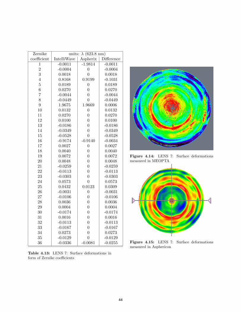
Zernike units: λ (623.8 nm)coefficient IntelliWave Aspherix Difference
1 -0.0011 -1.9814 -0.00112 -0.0004 0 -0.00043 0.0018 0 0.00184 0.8168 0.9199 -0.10315 0.0189 0 0.01896 0.0270 0 0.02707 -0.0044 0 -0.00448 -0.0449 0 -0.04499 1.9675 1.9669 0.000610 0.0132 0 0.013211 0.0270 0 0.027012 0.0100 0 0.010013 -0.0186 0 -0.018614 -0.0349 0 -0.034915 -0.0528 0 -0.052816 -0.9174 -0.9140 -0.003417 0.0027 0 0.002718 0.0040 0 0.004019 0.0072 0 0.007220 0.0048 0 0.004821 -0.0259 0 -0.025922 -0.0113 0 -0.011323 -0.0303 0 -0.030324 0.0573 0 0.057325 0.0432 0.0123 0.030926 -0.0031 0 -0.003127 -0.0106 0 -0.010628 0.0036 0 0.003629 0.0004 0 0.000430 -0.0174 0 -0.017431 0.0016 0 0.001632 -0.0113 0 -0.011333 -0.0167 0 -0.016734 0.0273 0 0.027335 -0.0129 0 -0.012936 -0.0336 -0.0081 -0.0255
Table 4.13: LENS 7: Surface deformations inform of Zernike coefficients
Figure 4.14: LENS 7: Surface deformationsmeasured in MEOPTA
Figure 4.15: LENS 7: Surface deformationsmeasured in Asphericon
44

(a) SAG error+residuals (Intellium) (b) IRR (Intellium)
(c) RSI + residuals, (Intellium) (d) RSI without residuals (Intellium)
Figure 4.16: LENS 7: Standard deformation errors
Tolerance for aspherical surface deformations is prescribed in an optical drawing of the lens. A-
ccording to the technical standards, deformations are represented by three errors:
Units: λ=632.8 nm
Asphericon MEOPTADrawing
tolerance
SAG PV 0.5694 0.3406 1.726
IRR PV 0.3409 0.2875 0.4315
RMSi 0.0475 0.0624 0.3452
RSI 0.0863 0.2491 0.2589
RSI-residuals 0.07
Table 4.4: LENS 7: Surface errors compared to optical drawing
SAG
SAG(Saggita error): The tolerance
on power of the surface (4th Zernike
coefficient) with respect to the refer-
ence sphere.
IRR
IRR (Irregularity): The tolerance on
the surface form error which remains
after the saggita error has been re-
moved, the PV with respect to the
best fit reference sphere.
RSI
RSI (Rotationally symmetric irregularity): The tolerance on the rotationally symmetric component
of the surface form error after the best fit sphere has been subtracted.
Values available from Asphericon are expressed in fringes of λ=546.07 nm, but Intellium interfer-
ometer works with λ=632.8 nm. Asphericon values were recalculated for chosen common units -
λ=632.8 nm.
45

Ge lens
Best F# 3.3Best fit position 191.1 mm
Reflected beam diameter 58.849 mmPixels 904OPD (normal direction) PV=10.5801 λ, RMS=3.3646 λOPD (ray tracing) PV=9.5301 λ, RMS=3.3135 λMeasured diameter 35/35 mmMeasurement range 3.3: 188.4-202.4 mm
Table 4.5: Ge lens: Output from Aspherix program
Transmission sphere
Asphere
-20
0
20
40
60
80
100
120
140
-50 -40 -30 -20 -10 0 10 20 30 40 50
Layout
IncidentReflected
Figure 4.17: Ge lens: Raytraced test arm of Intellium interferometer
46

0.00.020.040.060.080.1
0.120.140.160.18
Ang
le[◦
]
-20 -15 -10 -5 0 5 10 15 20Radial coordinate [mm]
Angle of incidence on aspherical surface
-1.0-0.8-0.6-0.4-0.20.00.20.40.60.81.0
Dev
iatio
nfr
omor
igin
alpo
sitio
n[m
m]
-40 -30 -20 -10 0 10 20 30 40Original ray position [mm]
Ray height differences on the reference surface
-10
-8
-6
-4
-2
0
[λ]
0 200 400 600 800 1000Pixels
Optical path difference
Nyquist limit
Nyquist limit-0.6
-0.4
-0.2
0.0
0.2
0.4
0.6Sl
ope
[λ]
0 100 200 300 400 500 600 700 800 9001000Pixels
Wavefront slope
Figure 4.18: Ge lens: Graphical output from Aspherix program
47

Zernike units: λ (623.8 nm)coefficient IntelliWave Aspherix Difference
1 0.1318 -6.32852 0.13182 -0.0000 0 03 0.0000 0 04 -3.2057 0.33153 -3.53725 -0.0090 0 -0.0096 0.0419 0 0.04197 -0.5481 0 -0.54818 -0.7643 0 -0.76439 4.2365 6.32882 -2.092310 -0.0019 0 -0.001911 -0.0122 0 -0.012212 0.0188 0 0.018813 -0.0010 0 -0.001014 -0.1000 0 -0.100015 -0.1150 0 -0.115016 0.4360 -0.31917 0.755217 0.0048 0 0.004818 -0.0135 0 -0.013519 -0.0018 0 -0.001820 0.0058 0 0.005821 0.0032 0 0.003222 0.0260 0 0.026023 -0.0322 0 -0.032224 -0.0212 0 -0.021225 0.1079 0.01186 0.09626 -0.0020 0 -0.002027 0.0012 0 0.001228 0.0014 0 0.001429 -0.0058 0 -0.005830 0.0180 0 0.018031 0.0093 0 0.009332 -0.0070 0 -0.007033 -0.0017 0 -0.001734 -0.0308 0 -0.030835 -0.0160 0 -0.016036 0.0088 -0.00021 0.009
Table 4.19: Ge lens: Surface deformations in form of Zernike coefficients
Figure 4.20: Ge lens: Wavefront measured on Intellium
48

4.7 Discussion
As Figure 4.14 and Figure 4.15 indicate, asphere LENS 7 was successfully measured with proposed
non-null testing method. In general, the results on surface tolerances from MEOPTA and Aspheri-
con in Table 4.4 do not differ by more than 0.2 λ. The considerable difference in case of Rotationally
symmetric irregularity can be explained by the number of Zernike polynomials used for calculating
RSI. In Asphericon, RSI PV was probably calculated only from the first four rotationally sym-
metrical terms. In order to check this, fit residuals were subtracted from the reconstructed OPD
and displayed RSI value became a sum of first four polynomials. Both RSI errors are only 0.01 λ
different. However, when describing surface deformations, it is not reasonable to restrict the num-
ber of used Zernike polynomials to standard 36 polynomials. Our previous experience in optical
testing suggests that most of the surface deformations can be described by higher order rotationally
symmetric Zernike coefficients. Because of this fact, IRR and RSI should have similar values, which
was confirmed in the measurement.
Visually comparing surface deformations, both have the same looking central part surrounded by
four annular lower valued zones. Although PVs are slightly different, the structure of the surfaces
is similar.
To sum up, interferometric measurements revealed that this asphere was manufactured correctly;
none of the errors exceeds the value allowed in the drawing. LENS 7 can be measured on Intellium
Fizeau interferometer in MEOPTA even without any additional hardware optimized for measure-
ments of aspheres.
On the other hand, non-null measurements of Ge lens show a mismatch between theoretical
prediction and experimental data. For example, there is still 2 λ in primary spherical aberration
which was supposed to be subtracted from the measurement. Such high value means that mea-
surements are influenced by factors which were not previously considered. In case of LENS 7, the
unknown error is not significant to the measurement; the accuracy of results is comparable to the
accuracy of stitching interferometer. Non-null testing method described in this chapter is simplified
by neglecting the influence of retrace error, hence it is probably the cause of problems in Ge lens
measurement. In further research, instead of measuring more aspheres, we decided to focus on
explanation how retrace error can change the non-null testing results.
49

Chapter 5
Retrace Error
Asphere
Sphere
Figure 5.1: Non-null testing of an asphere; incidentand reflected rays have the different paths
Creating a reference wavefront that matches the
test surface is a goal in the interferometric null
tests. If the null condition is met, both test
and reference beam follow the common path
through the interferometer optics. Null tests
are normally implemented to test spherical op-
tics, since the accurate reference objective can
produce an almost perfect spherical wavefront.
Measurement inaccuracy that results from fail-
ure to meet null condition is commonly referred
to as retrace error. Retrace error will always
be present if a sphere is replaced by an asphere
while having the spherical reference wave.
We recognize two types of retrace error: retrace path error and retrace surface error [40]. Re-
trace path error is caused by test ray following the different path than reference ray. It is no longer
possible to image the point source on itself, thus the aberrations of the interferometer system do
not cancel out like they do when rays follow the same path. Moreover, the surface under test is
not manufactured perfectly; its deformation will further change the path of incident rays and cause
what we call retrace surface error. This error is unpredictable, so we can only assume it is negligible
when the surface is well manufactured.
One of the first papers on this topic was published in 1992 [41]. The large spherical aberration
of one lens from Hubble space telescope was double checked using different interferometers. The
authors noticed an unexpected increase in spherical aberration after displacing the test lens from
the null position. The initial reason to move the Hubble lens was to stop overfilling the reference
mirror aperture.
An article by Kreischer [42] written from the point of view of optical designer studies the retrace
50

error as a function of transmission sphere design. Retrace error with regard to testing nominally
spherical surfaces is largely ignored, but its influence can be significant when high test accuracy is
needed. Author identifies two types of retrace error: Axial; induced spherical aberration resulting
from defocus, and Transverse; induced coma as a result of tilt. Both of them were taken into account
while designing a new transmission sphere. As results suggest, lower F#, the higher the retrace
error. All Kreischer optics transmission spheres were adequately corrected to minimize the effect of
retrace error.
In the previous chapter, we present the results of non-null measurement of aspheres using Fizeau
interferometer. As comparison with stitching interferometer shows, we were successful in case of
LENS 7, however, measurement of Ge lens raised a question about the influence of retrace error.
This chapter will study the retrace error and give an explanation why the retrace error plays an
important role in data analysis from non-null measurements. The possibilities of removing retrace
error will be suggested based on experimental and theoretical results.
Experimental approach was used for retrace error evaluation on Intellium Fizeau Z100 inter-
ferometer. Since the manufacturer refused to reveal parameters of transmission spheres or inner
lenses, comparison with theoretical predictions was not possible. It was obvious we would receive a
negative reply; ESDI company also sells special Fizeau interferometer Intellium Asphere intended
for testing of aspheres. Its parameters do not differ from the Z100 model, it even has two transmis-
sion spheres ∅100 mm with F#s 0.75 and 1.5 included. The newer version of IntelliWave software
can compensate for retrace error and the dynamic range of the interferometer is increased by using
Sub-Nyquist algorithm.
Behavior of retrace error for aspheres was estimated using the simulation with sphere. Sphere with
radius of curvature r=19.768 mm was defocused from the best fit position and retrace error was
calculated.
The retrace error can be also influenced by using built-in optical zoom, which makes the change in
the interferometer setup. Results for Ge lens with and without zoom are compared.
Alongside, theoretical calculations were done on brand new Twyman-Green interferometer, com-
pletely designed in MEOPTA. The custom-made components meet all the standards for optical
testing. This time, the reference surface is not spherical, but a plane mirror which is much easier
to manufacture. Up to the present time, this interferometer is not constructed, but we benefited
from the knowledge of the nominal design and checked the options for testing of aspheres. With a
full prescription of the system, retrace error for aspheres could be precisely analyzed in lens design
software.
5.1 Experimental Approach
The origin of retrace error was already explained, so the important issue to solve was how to quan-
tify it. It was done by comparing the changes of OPD in the detector plane with OPD in normal
51

direction. Experimental data from IntelliWave software of Intellium Fizeau interferometer show half
of the double pass OPD, and, in case of null testing, it is the topography of the tested surface. In
non-null configuration, with increasing deviations from normal incidence, paths of the reflected rays
are differing more from the incident ones. Dividing the total OPD into half does not give correct
image of what we want to measure: normal direction OPD between the aspherical surface and the
reference sphere. Therefore, retrace error can be quantified as a difference between experimental
data and theoretical prediction of OPD computed in normal direction. Theoretical calculations
were done in Octave program Aspherix.
The spherical surface with radius of curvature r=19.768 mm was defocused ± 0.05 mm from
the null position. Theoretical Zernike coefficients are the wavefront aberrations in normal direction
between sphere defocused copy. Aspherix program also calculates how much of the spherical diam-
eter is actually imaged on the detector; a transmission sphere F#=3.3 is not enough to illuminate
the entire diameter.
Another experiment was carried out to check if Intellium built-in optical zoom has an influence
on measurements. Ge lens measured in Table 4.6 was used as a test subject. The reflected beam
diameter in the best fit position is smaller than aperture of the transmission sphere, thus it was
possible to zoom in and zoom out. Reconstructed OPD maps for all cases are compared.
Results
19.7 19.72 19.74 19.76 19.78 19.8 19.82 19.84
−0.1
−0.05
0
0.05
0.1
0.15
0.2
0.25
0.3
Null position
Retr
ace e
rror
[λ]
Distance from the center of curvature [mm]
4 Focus
9 Spherical
16 Spherical
25 Spherical
Figure 5.2: Retrace error for defocused sphere with r=19.768 mm
52

The graph in Figure 5.2 indicates that retrace error has an influence on focus and primary spher-
ical aberration, the other rotationally symmetrical Zernike coefficients change is almost zero, it lies
below 0.05 λ. Focus aberration is the Zernike term mostly influenced by retrace error. Growth of
the primary spherical aberration is symmetrical on both sides.
As can be seen from Figure 5.2, the experiment with defocused sphere suggests that retrace error
causes a rather slow increase in primary spherical aberration (less than 0.1 λ for 0.05 mm of defocus).
LENS 7 with very low aspherical coefficients can be approximated by sphere, so we can estimate
the retrace error using the graph for defocused sphere. In this case, it is almost null measurement
and retrace error is negligible. Ge lens has around three times higher deviation from sphericity than
LENS 7 and, in this case, retrace error changes the detected wavefront.
Figure 5.3 confirms that, for asphere, using the optical zoom in non-null measurements can signifi-
cantly change the shape of detected wavefront, thus also the retrace error. Zooming means changing
position of one of interferometric imaging lenses, so the wavefront is modified. Zooming in decreases
the detected spherical aberration, zooming out increases.
5.2 Theoretical Approach
Prescription of all components of Twyman-Green interferometer is available in optical design soft-
ware Zemax. We can check suitability of this tool for measurements of aspheres and how the retrace
error affects the detected OPD. The general task stays the same as it was with Fizeau interferometer
- to find the best measurement configuration. The solution is found using Zemax optimization tool.
This time, the only variable in the system is position of the asphere, the transmission sphere is fixed
(F#=1.2). More transmission spheres are yet to be designed. Our request is to measure retrace
error, so detected OPD is compared to OPD in normal direction computed in Aspherix program.
53

-2
0
2
4
6
8
[λ]
0 100 200 300 400 500 600 700Pixels
Optical path difference
(a) OPD with minimal zoom
-3-2-101234567
[λ]
0 200 400 600 800 1000 1200 1400 1600Pixels
Optical path difference
(b) OPD with maximal zoom
-2
0
2
4
6
8
[λ]
0 100 200 300 400 500 600 700 800 900Pixels
Optical path difference
(c) OPD without zoom
Figure 5.3: Ge lens measurement: results with zoom
minimal zoom without zoom maximal zoom
pixels 665 880 14764 Focus -4.0726 -3.2057 -2.0217
9 Spherical 3.2584 4.2365 5.0543
Table 5.4: Ge lens measurement: results with zoom
54

Figure 5.5: Twyman-Green interferometer with the tested surface in cat’s eye position
55

Results
Asphere A3
Measured ∅ Complete ∅20.1437 mm 23 mm
Zemax best fit Aspherix best fit33.023 mm 32.461 mm
Zemax OPD Aspherix OPDPV=79.052 λ PV=79.079 λ
Zemax Aspherix Retrace error
4 Focus -45.1593 -39.5602 -5.59919 Spherical 6.5656 16.1259 -9.560316 Spherical 8.2311 1.00138 7.229725 Spherical 2.7867 0.1443 2.642436 Spherical 0.5919 -0.0026 0.5945
Table 5.1: Retrace error for asphere A3 measured on Twyman-Green interferometer
Asphere A4
Measured ∅ Complete ∅10.494 mm 22 mm
Zemax best fit Aspherix best fit15.521 mm 15.62 mm
Zemax OPD Aspherix OPDPV=3.95 λ PV=3.6448 λ
Zemax Aspherix Retrace error
4 Focus -0.2335 -0.8989 0.66549 Spherical 2.4825 1.7806 0.701816 Spherical 0.3699 0.0028 0.367125 Spherical 0.0526 0.002 0.050636 Spherical 0.008367 -0.00003 0.0084
Table 5.2: Retrace error for asphere A4 measured on Twyman-Green interferometer
Figure 5.6: Interferogram for asphere A6; rays reflected from the middle part are cut off by system apertures
56

Overall, Zemax simulations showed that this interferometer with F#=1.2 is not a good instru-
ment for testing of aspheres. Aperture of the transmission sphere is insufficient to illuminate entire
diameter of tested surface. Due to short focal distance, aspheres with large vertex radius of cur-
vature cannot be placed in the best fit position (eg. LENS 7, Ge lens). With F#=1.2, the part
of reflected aspherical wavefront does not even reach the detector in most of the cases (the typical
interferogram looks like Figure 5.6). However, the biggest problem is insufficient chip resolution.
Asphere A3 example is shown as a typical case. Even when the position where most of reflected
rays reach the detector is found, wavefront slope still violates the Nyquist condition. Aspherical
departure from the planar wavefront reaches usually around 70 λ. As Table 5.2 shows, aspherical
wavefront changed its shape after passing interferometer optics; higher order aberrations become
more important. Retrace errors are obviously large as well when the shape of the wavefront becomes
completely different. The only asphere which can be measured using Twyman-Green is A4, but
only around half of its diameter. This asphericity will still cause retrace errors 0.7 λ for primary
spherical aberration. At Twyman-Green interferometer, retrace error is not negligible even when a
wavefront with low asphericity is imaged.
Possible upgrade to make this setup more suitable for measurement of aspheres is using a different
transmission sphere with higher F# or detector with higher resolution.
5.3 Discussion
To sum up, all previous results confirm non-null testing method can give satisfying results only in
case of weak aspheres. The only lens successfully measured on Intellium Fizeau interferometer is
LENS 7, which has the lowest coefficients of asphericity from all the aspheres in MEOPTA. For the
rest, disadvantages of non-null testing become significant. The deviation of reflected rays from the
incident ones might cause they do not reach the detector at all. In the opposite case, they take a
different path in the imaging optics and add up system aberrations to the wavefront. Indeed, retrace
error has an impact on results in non-null measurement of aspheres and it definitely needs to be
considered in data analysis. In the measurement of aspherical surface of LENS 7, it can be neglected
due to fortunate combination of conditions: big vertex radius of curvature and low asphericity. All
together, we came to the conclusion that full prescription of the optics inside measuring instrument
is absolutely necessary for testing of aspheres. As predicted, moving one lens in the interferometer
(zooming) proves that retrace error affects the results.
It is clear that interferometer must be calibrated for useful measurements of aspheres. The
Aspherix program can be a starting point for writing macro in Zemax programming language which
can calculate the optimal measurement conditions. With the full knowledge of system parameters,
the detected wavefront shape can be predicted and separated from measurements. Influence of
retrace error will be included in final OPD after an entire system is raytraced.
More simulations need to be done to find out how much tilt and decenter of optical elements in-
57
fluence the final OPD. More accurate calibration method which we suggest to use in the future is
reverse optimization. The conventional task for lens design program is to find the system parame-
ters which meet the designer’s requirements for the system performance. In reverse optimization,
the real system performance is measured first. Zernike coefficients of OPD are set as optimization
operands together with tilts and decenters of elements, position of test surface. Afterwards, the
optimization process adjusts the variables in order to reach the minimal deviation between actual
and measured OPD. Parameters of the interferometer optics must be known better than their design
prescriptions and tolerances allow to achieve more accurate results.
Since interferometric testing with non-adapted wavefront was not proven as reliable and universal
method, we decided to invest the time into designing a null compensator. If it is possible to design
it in a simple way and the compensation is efficient, the advantages of having accurate method to
test important aspheres outweigh the cost and designing difficulties.
58

Chapter 6
Null Testing
As discussed in the previous chapter, retrace error has a significant influence on the results in non-
null aspherical testing. Since we are not able to exactly quantify its influence in testing of aspheres
on Intellium interferometer, the concept of null testing which seemed nontrivial is now reconsidered
as next method to try. The designed null component should minimize differences between reference
and reflected wavefront. The compensator modifies the paths of rays and shapes the transmitted
wavefront. This results in the incident rays reaching the aspherical surface in the normal direction,
following the same path on the way back. For this reason retrace error approaches zero and does
not have to be considered in further analysis. In the ideal case, all system optics aberration cancel
out and have no effect on the measurement.
Simple null compensators consisting of only one lens were designed for aspheres available in MEOPTA.
The results are presented in this chapter.
6.1 Optical Design and Tolerancing
Up to the late 1940s, all optical designs had to be made by hand calculation. This method was very
tedious and time-consuming. Probably the earliest use of a computer to trace rays was by James
G. Baker in 1944, who used the Mark I calculator at Harvard to trace rays. Later on, with the start
of computer era, faster computations opened the new possibilities in the lens design. Even after the
years of development, present lens design programs are still far from being completely automatic.
The experience and proper knowledge are essential to operate them correctly.
Optical components are designed using the program’s optimization tool. The optimization func-
tion takes a starting design and modifies its construction so that it meets a given set of specifications.
The starting design may be the result of a previous design task, combination of catalog lenses or a
brand new design based on the designer’s experience and intuition. The performance of the design
is evaluated by outcome of single error function called merit function. The merit function is the
sum of squares of desired system attributes called operands. It can be defined in many manners,
e.g. geometrical spot size, root mean square deviation of detected wavefront or desired behavior
of modulation transfer function. The operands put the constraints on the system performance.
59

Typical operands are, for instance, the maximal value of spherical aberration, ray heights of certain
rays, exact value of focal distance.
The program iteratively adjusts the system constructional parameters - radii of curvature, glass
thickness, diameters, coefficients of asphericity, refractive index, etc. The optimization process
uses them as variables and finds the solution which collectively minimizes the deviations of actual
operand values from the target. It is not very probable that solution makes all of the operands equal
to their target values. The importance of each operand forming the merit function is controlled
by weight factors. Not all of the operands need to be exactly satisfied. If the factor is larger, the
variables affecting the operand do not change a lot. Obviously, the variables affecting the operand
with smaller weights can get values far from the initial guess.
Usually the operands depend on the given variables nonlinearly. From the mathematical point
of view, this property leads to difficult nonlinear least-squares optimization. The final solution of
nonlinear equations depends on the initial conditions, so well chosen input values can considerably
reduce the computation time. Unfortunately, the program cannot find the global minimum, it finds
the local minimum influenced by initial conditions. Sometimes the system reaches the stagnation
point where the program cannot find any solution independently of number of iterations. The merit
function value does not seem to change and minimization is too low to be helpful. To overcome this
issue, the different initial conditions have to be entered to the program.
The optical design does not finish with the successful optimization. In reality, the optical and
mechanical components can never be made perfectly, so determination of the tolerance upon the
system is even more important task. The system must keep a good performance when the variables
have the values in the reasonable range. The tolerances for dimensions and product properties are
a part of the standardized way of communication between the optical designer and the technologist.
Without a standard method for describing the details of the part, there is no guarantee that the
designer will end up with a part which matches his/her specifications [43].
The most commonly used standard in the industry is ISO 10110. It describes the preparation
of drawings for optical elements and systems. Each part covers a different aspect of the optical
drawing. Typical manufacturing tolerances in a lens system are listed in Table 6.1.
Parameter Commercial Precision High precision
Wavefront residual RMS 0.25 λ 0.1 λ <0.07 λThickness 0.1 mm 0.01 mm 0.001 mmRadius 1 % 0.1 % 0.01 %Index of refraction 0.001 0.0001 0.00001Abbe number 1 % 0.1 % 0.01 %Decenter 0.1 mm 0.01 mm 0.001Tilt 1’ 10” 1”Sphericity 2 rings 1 ring 0.25 ringIrregularity 1 ring 0.25 ring <0.1 ring
Table 6.1: Typical values of tolerances in a lens system [3]
60

6.2 Null Compensators for Aspheres
The very best option for null testing is having a reference surface for comparison. The quality of
the reference needs to be better than quality of any tested surface. Unfortunately, aspherics with
sufficient quality cannot be manufactured in MEOPTA yet. The degree of compensation of wave-
front aberrations depends on the quality of all surfaces involved. Deformations of spherical/planar
surfaces can be easily checked using interferometers, so it is preferable to design a compensating
element without special surfaces. MEOPTA usually reaches λ/20 precision for spheres and λ/30
for planes, which is sufficient for null measurements.
Another aspect to consider was whether the compensator should be reflective or refractive. It
would be difficult to set correct off-axis alignment with the equipment available in the laboratory, so
there are two possibilities of our next approach. The first one is to put the aspherical lens in between
the transmission sphere and compensating mirror. The other one requires refractive compensating
element and aspherical surface is measured in reflection. The second option was chosen because it is
easier for the optimization. In the first one, there are only four parameters to vary - the position of
the aspherical lens (distance to transmission sphere and to the reflective compensator), orientation
of aspherical lens (which surface refracts first) and the radius of curvature of the mirror. While
designing the refractive null compensator as sigle refractive element, apart from its position in the
setup we can alter both radii, the lens thickness and the glass type. With more parameters to
change, there is a higher chance that a combination, which meet our demands, exists.
Generally, our goal is to design sufficient null compensator as simple as possible. The compen-
sating element was designed using optical illumination software Zemax using its extensive built-in
optimization and tolerancing tools. We assume that the greater part of the aberration introduced
by the asphere is of low order. This condition makes it easier to get good compensation with a
single element of convenient form. For this reason our compensator consists of only one lens with
planar/spherical surfaces manufactured from the common type of optical glass BK7.
Spherical reference optics used with Fizeau interferometer was replaced by perfect lens in the
simulations because the exact transmission sphere design is not available. The double-pass system
was optimized for compensator radii, thickness and compensator position between the asphere
and transmission sphere. All three transmission spheres were considered. It is required that the
compensation must work well for entire diameter of aspherical surface. This condition seems very
strict for aspheres strongly differing from spheres or with large diameter.
61

6.3 Optimization Results
Optimization was successful for three out of ten aspheres available. LENS 7 was not included since
it was proven no compensating elements are necessary to measure the topography of the aspherical
surface. As predicted, it was not possible to compensate strongly apherical wavefronts. All three
lenses have one common feature - big radius of curvature (A1:ra=-185.5253 mm, A8: ra=164.3958
mm, A11: ra=184.882 mm). They make the least aspherical wavefront after the reflection. It seems
like the coefficients of asphericity do not have as big influence in the optimization process as the
radius of curvature. Actually, the asphere A1 has one of the highest coefficients A2 = 8.9.10−5.
A1 compensating element works as a diverging lens, the rest is converging (A1 is a concave surface
and it focuses the reflection). We found out that the objectives available for measurements are not
sufficient to approach the normal incidence of incident rays. Using the transmission sphere with
higher F# would lower the angle of incidence (without using additional lens).
The compensator shapes and positions are shown below. The wavefront errors after the compensa-
tions are less than 0.035 λ, the residual spherical aberration is less than 0.02 λ.
62

Figure 6.1: A1 null compensator placed in the correct position
Figure 6.2: A1 null compensator
Figure 6.3: Residuals after compensation of asphericity
63

Figure 6.4: A8 null compensator placed in the correct position Figure 6.5: A8 null com-pensator
Figure 6.6: Residuals after compensation of asphericity
64

Figure 6.7: A11 null compensator placed in the correct position
Figure 6.8: A11 null compensator
Figure 6.9: Residuals after compensation of asphericity
65

Asphere A1 (in the drawing named as LENS 6) has the highest asphericity out of three aspheres
for which the compensating element was designed. For this reason, the compensator for LENS 6
was the one chosen to be manufactured.
R=∞ R=6.982
4.3
12 14
Figure 6.10: Null compensator for LENS 6
6.3.1 Reflectivity of Aspherical Surface
In suggested null configuration, the aspherical surface is a reflective component, so it is necessary
to characterize its reflectivity. Fizeau interferometers generate an interference between the surface
of a test sample and a reference surface. The interference image is recorded and analysed by an
imaging optics system. The contrast of the interference signals depend, however, on the reflectivity
of the test samples. Both beams should have similar intensities to get high contrast of fringes. The
reference beam is reflected from the last surface of the transmission sphere. There is no antireflection
coating; the standard glass-air interface reflectivity is around 4 %. According to optical drawing,
both surfaces of aspherical lens are antireflection coated for the wavelengths ranging from 650
nm to 950 nm. A manufacturer claims that maximum reflectivity is in this range is 0.5 % for the
aspherical surface and 1 % for the spherical surface. Luckily, the antireflection coating was optimized
for central wavelength around 800 nm and quite broad bandwidth, which most likely indicates the
quick increase of reflectivity outside the bandwidth. The reflectivity of LENS 6 aspherical surface
for the wavelength we use for testing (632.8 nm) is not known, but as measurement showed, it is
sufficient to give a good contrast of interference fringes.
6.3.2 Tolerance Analysis
The result of optimization with very precisely calculated values of radii, glass thickness and dis-
tances needs to be adjusted; in reality, such high precision is not possible to reach.
The radii of curvature were not chosen arbitrarily. There is a finite number of optical calibers
according to CSN 19 0425 standard, so choosing the radius from the catalog would speed up the
66

manufacturing process. One of the radii is replaced by the most similar radius from the catalog and
the system is re-optimized with the same conditions. Then, the other radius is fixed to the catalog
value and again, the optimization with the remaining variables is done. This manual iterative pro-
cess finishes when the best combination of catalog radii is found.
Tolerance analysis is important to set limits for the manufacturing process. As a first step, con-
straints on the radii of curvature, glass and air thicknesses, refractive index and Abbe number of
the glass were set. Any change in one of the parameters can be later still optimized by readjusting
the position of entire mechanical device.
Tolerance for tilts and decenters in the system was examined separately. The system was tolerated
for centricity of compensating lens (TUTX 4, TUTY 4), centricity of the asphere (TUTX 9, TUTY
9, 1’ from the drawing), decenter and tilt between optical axes of both lenses (TUDX 2, TUDY 2).
Compensation is considered as sufficient if the RMS value of the residuals does not exceed 0.1 λ.
TFRN 3 Tolerance on second radius of curvature of compensating lens ±4 fringesTFRN 4 Tolerance on aspherical radius of curvature (from the drawing) ±4 fringesTTHI 2 Glass thickness ±0.05 mmTTHI 3 Air thickness between compensator and asphere ±0.1 mmTIND 2 Refractive index of glass ±0.0005TABB 2 Abbe number of glass ±1 %
Table 6.2: Tolerances for the compensating element of LENS 6
Tolerance analysis shows that the most critical parameters are the distance between compensator
and asphere. RMS is also very sensitive to any decenter between lenses. A solution how to fix the
position and make the optical axes aligned is placing the lenses in mechanics.
67

Analysis of Tolerances
Criterion : RMS Wavefront Error in waves
Nominal Criterion : 0.00496883
Test Wavelength : 0.6328
Worst offenders:
Type Value Criterion Change
TTHI 3 1 -0.10000000 4.66115086 4.65618203
TTHI 3 1 0.10000000 4.56037073 4.55540190
TFRN 4 -4.00000000 1.35100480 1.34603597
TFRN 4 4.00000000 1.31061294 1.30564411
TIND 2 -0.00050000 0.91593884 0.91097001
TIND 2 0.00050000 0.89803453 0.89306571
TTHI 2 1 -0.05000000 0.89479926 0.88983043
TTHI 2 1 0.05000000 0.87996965 0.87500082
TFRN 3 -4.00000000 0.61844430 0.61347547
TFRN 3 4.00000000 0.60327253 0.59830370
Monte Carlo Analysis:
Trial Criterion Change Optimized
1 1.30216886 1.29720003 0.028
2 0.88906268 0.88409385 0.0348
3 3.42563422 3.42066540 0.126
4 0.61103685 0.60606802 0.0762
5 0.19875382 0.19378499 0.10004
6 1.96898499 1.96401616 0.0102
7 0.11038697 0.10541814 0.0078
8 1.89896362 1.89399479 0.0417
9 2.12090128 2.11593245 0.0077
10 3.29636401 3.29139518 0.041
11 1.09133173 1.08636290 0.0148
12 0.25056829 0.24559946 0.0251
13 3.29598691 3.29101808 0.0889
14 1.71214128 1.70717245 0.0577
15 2.26746571 2.26249688 0.0108
16 0.82883917 0.82387034 0.0106
17 2.32731092 2.32234209 0.0599
18 0.49317647 0.48820764 0.0568
19 1.09628864 1.09131981 0.0215
20 4.28540222 4.28043339 0.0029
Table 6.3: Tolerance analysis results (without tilts and decenters)
68

Analysis of Tolerances
Criterion : RMS Wavefront Error in waves
Nominal Criterion : 0.00496883
Test Wavelength : 0.6328
Worst offenders:
Type Value Criterion Change
TUDX 2 0.01000000 0.31519090 0.30529674
TUDX 2 -0.01000000 0.31519090 0.30529674
TUDY 2 0.01000000 0.31519089 0.30529673
TUDY 2 -0.01000000 0.31519089 0.30529673
TUTY 9 0.02000000 0.12176943 0.11187527
TUTY 9 -0.02000000 0.12176943 0.11187527
TUTX 9 0.02000000 0.12176943 0.11187527
TUTX 9 -0.02000000 0.12176943 0.11187527
TUTX 4 0.02000000 0.07743054 0.06753639
TUTX 4 -0.02000000 0.07743054 0.06753639
Monte Carlo Analysis:
Trial Criterion Change
1 0.20552623 0.19563207
2 0.26597284 0.25607869
3 0.07324431 0.06335015
4 0.20449178 0.19459763
5 0.12546117 0.11556702
6 0.22529735 0.21540319
7 0.18483055 0.17493639
8 0.21393267 0.20403851
9 0.22702532 0.21713116
10 0.14652946 0.13663530
11 0.04407165 0.03417750
12 0.27640221 0.26650805
13 0.35975181 0.34985766
14 0.39198553 0.38209137
15 0.39893056 0.38903641
16 0.20577322 0.19587906
17 0.09236110 0.08246694
18 0.04795040 0.03805625
19 0.09988498 0.08999082
20 0.28468267 0.27478852
Table 6.4: Tolerance analysis results (tilts and decenters)
69

6.3.3 Mechanics for Null Component
In practice, the desired distance between the components in the null measurement is difficult to
reach. Eliminating tilt and decenter in the system is even more complex task to solve. As a result,
the mechanical device was designed in MEOPTA to remove some degrees of freedom for the final
null testing. Both lenses (compensating lens and asphere) are inserted into a custom-made tube
(Figure 6.11). Its design and dimensions were chosen to keep the distance between the lenses fixed
for 14.63 mm. Zemax tolerance analysis in Table 6.3 also confirms that this distance is the worst
offender in tolerencing process, that is why the mechanical tolerance for set for ±0.01 mm.
At first, the compensating lens is centered to the outside diameter of the tube. The non-centricity
of the lens itself must be as low as possible, the mechanics cannot compensate for it. Next, the lens
is cemented in the best centered position, which is why the tube has three side holes.
The aspherical lens is removable for the purpose of optical testing. Nevertheless, it needs to be
fixed in the tube and properly aligned with the compensating lens. Its position in the mechanics is
set by two rings placed on the edge of the spherical surface. One of them is held by the external
thread in the tube. We assume that asphere itself has zero centricity error.
The tube is made of free-cutting steel with material number 1.0715, all the surfaces are blacked to
suppress any stray light reflections. The material is described as free-cutting steel for bulk appli-
cations for joining elements in mechanical engineering and automotive components [44]. The ring
touching the spherical surface is made of flexon to prevent the damage, the threaded one is made
of alloy.
The only degrees of freedom left now are the tilt, decenter and position of the entire device.
Unfortunately, tolerance analysis shows that even very strict constraints for surface tilts (1’) and
decenters (0.01 mm) cross the limit of resulting RMS=0.1 λ. The tilts and decenters of lenses
with respect to the axis of mechanical device need to be measured and later subtracted from the
measurement.
70

Figure 6.11: Mechanical device for null measurement, complete drawing is in Appendix D
Simple refractive null compensators for three aspheres were designed in Zemax. When they
are placed in between the transmission sphere of Intellium interferometer and tested asphere and
properly aligned, they should compensate the asphericity of detected wavefront. The PV of the
wavefront after compensation does not exceed to 0.04 λ. Compensator for LENS 6, in form of
plan-concave lens, is about to be manufactured and tested in the future. Mechanical device for
testing with this comensator was designed as well.
71

Chapter 7
Conclusion
This thesis reviewed the efficiency of technologies available in Optical metrology department in
MEOPTA for aspherical testing. The task required coding an own program in Octave for theoreti-
cal simulations, which were compared to experimental results.
Two devices were used for aspherical testing: Intellium Fizeau interferometer and HASO Shack-
Hartmann sensor. Their limitations were found by simulating the measurement in the Octave pro-
gram. A short list of aspherical lenses included in MEOPTA products was tested on both devices
and the performance of two different wavefront detection methods was analyzed. Phase shifting
interferometry was suggested to be used in the future experiments due to its higher dynamic range
and better spatial resolution.
Method for testing aspheres with spherical reference on Intellium interferometer was proposed in
this thesis. Analysis of surface deformations relies on the outcome of ray tracing simulation in
Octave program. The program provides the wavefront to be subtracted from the wavefront recon-
structed by IntelliWave software using phase shifting method. Theoretical predictions suggested
two aspheres from the list that could be measured in non-null setup.
The results were positive in case of asphere LENS 7, which has the lowest coeffiecient of ashericity
from all available aspheres. Surface deformations of the other lens, made from Germanium, were
not evaluated correctly. Even though a wavefront reflected from the test surface was successfully
reconstructed, a mismatch between observed shape and its theoretical prediction appeared. This
raised a question about the accuracy of simulation. The possible missing factor which was not con-
sidered is the influence of retrace error - aberrations introduced by interferometer optics in non-null
testing setup.
Since it was not possible to work with prescription of Intellium interferometer optics, retrace error
was not precisely quantified. Simulations on Twyman-Green interferometer, soon to be assembled
in MEOPTA, showed that retrace error cannot be neglected and it has a strong impact in non-null
testing of aspheres. Using Intellium Fizeau interfemeter with spherical reference beam is a good
option for aspherical testing only for very weak aspheres (with coefficient A2 ∼ 10−7). In general,
analysis of data from non-null testing requires the full information about the system which must be
72

completely raytraced.
Testing aspheres with spherical wavefront was proven to be inefficient. Nevertheless, Intellium inter-
ferometer can still be used in the future with special beam shaping optics. Three simple refractive
null compensators were designed minimizing the asphericity of detected wavefront. Compensating
element for LENS 6 asphere in the shape of plan-concave lens is currently being manufactured and
will be tested afterwards. If the quality of surfaces is sufficient, it will be placed in a mechanical
device together with the asphere to fix their relative position. Then, if aspherical testing with null
compensator will give satisfying results, the benefits will outweigh the costs of manufacturing the
lens.
73

Appendix A
List of Aspheres Used in MEOPTA
za =1ra· S2
1 +
√1− (K + 1)
(1ra
)2S2
+4∑
i=1
AiS2i
A1 A2 A3
SPOJKA 6 ASF. LENS 1 LENS 6
730 0760 00111 07300760009110 07300760010110
Optical diameter d 11.4 22.8 23
Radius of curvature ra -185.5253 32.71039 30.89927
Conic constant K 0 -1.39446 0.36221
Coefficient of asphericity A1 0 0 0
Coefficient of asphericity A2 8.95734e-5 -1.165537e-5 -6.760244e-6
Coefficient of asphericity A3 0 -3.726022e-8 -3.420194e-9
Coefficient of asphericity A4 0 -7.747244e-11 -7.387291e-11
za =1ra· S2
1 +
√1− (K + 1)
(1ra
)2S2
+4∑
i=1
AiS2i
A4 A5 A6
LENS 1 - ASP LENS 4 - ASP LENS 6 - ASP
07300760006110 07300760007110 07300760008110
Optical diameter d 22 13.6 16.6
Radius of curvature ra 15.3817 43.947 -58.4325
Conic constant K -0.13889 -0.03818 0
Coefficient of asphericity A1 0 0 0
Coefficient of asphericity A2 -4.841939e-6 -4.076374e-5 -2.02409e-4
Coefficient of asphericity A3 5.833533e-9 -2.685245e-7 -2.625569e-7
Coefficient of asphericity A4 -1.673422e-10 -2.562076e-9 1.039743e-8
74

za =1ra· S2
1 +
√1− (K + 1)
(1ra
)2S2
+4∑
i=1
AiS2i
A7 A8 A9
LENS 8 ASPH LENS 4 LENS 7
730 0760 00488 730 0760 00288 730 0760 00388
Optical diameter d 11.4 28.9 35
Radius of curvature ra -24.43 164.3958 133.2126
Conic constant K -10 0 0
Coefficient of asphericity A1 0 0 0
Coefficient of asphericity A2 -3.0574139e-5 -1.16455137e-6 -2.6934596e-7
Coefficient of asphericity A3 7.3835473e-7 1.1766029e-10 4.0803344e-10
Coefficient of asphericity A4 0 0 0
za =1ra· S2
1 +
√1− (K + 1)
(1ra
)2S2
+4∑
i=1
AiS2i
A10 A11
ROZPTYLKA 5 Ge lens
760342
Optical diameter d 23 35
Radius of curvature ra -21.22 184.882
Conic constant K 0 0
Coefficient of asphericity A1 0 -4.725e-6
Coefficient of asphericity A2 4.13e-5 -2.972e-7
Coefficient of asphericity A3 0 5.26e-11
Coefficient of asphericity A4 0 0
75

Appendix B
Zernike Frindge Coefficients
Figure B.1: Page is from Intelliwave software manual [39]
76

Appendix C
LENS 7: Measurement Protocol from Asphericon
77

Appendix D
LENS 6: Mechanics for Null Compensator
B
B
2 31 4
2 31 4
C
B
D
E
A
F
C
B
D
E
A
F
FORMAT A4
---
DUVE
RNE
---
Tent
o do
kume
nt a
info
rmac
e v
nem
obsa
zene
jsou
duv
erne
ane
smi b
yt k
opiro
vany
ani jina
k re
prod
ukov
any
v ce
lku
nebo
z cas
ti be
zpr
edch
oziho
pise
mneh
o po
voleni s
polecn
osti
Meop
ta -
opt
ika, s
.r.o.
Copy
right
Meo
pta
- op
tika, s
.r.o., 20
11
---
CONF
IDEN
TIAL
---
This d
ocum
ent an
d info
rmat
ion
cont
aine
d with
in a
re c
onfid
entia
lan
d ma
y ne
ither
be
copied
or
othe
rwise
repr
oduc
ed in
who
le o
rin p
art
with
out
the
prior
writt
en a
ppro
val Me
opta
- o
ptika, s
.r.o.
Copy
right
Meo
pta
- op
tika, s
.r.o., 20
11
CAD: Creo Elements/Pro 5.0
Meopta - optika, s.r.o.Kabelikova 1, 750 02 PrerovCzech RepublicTel.: +420 581 24 1111www.meopta.com
0.01 A
NAMEDATEDESCRIPTIONCHANGENUMBER
INDEXQTY.VER.
x
x
x
1SHEETSP823106438502DRAWING NAMEmm/g/s/°CmKCSN ISO 2768 -
NON-SPECIFIED TOLERANCES ACCORDING TO
NEPREDEPSANE TOLERANCE DLE28.02:11SHEETP823106438502MODEL NAMEUNITS:WEIGHTSCALE
1ACUSTOMER NUMBERIng. SevcikPRODUCTIONAPPROVED
CUSTOMERSPECIFIED FOR RNDr. HrdaNORMALIZED
VERSIONPROJECTREPLACES VERSIONIng. LochmanAPPROVED
REPLACES DRAWINGIng. LochmanCHECKED TUBESEMIPRODUCTIng. LezakDRAWN
MATERIAL STANDARDIng. LezakDESIGNEDTUBUSTITLE
1.0715MATERIAL31.03.2014DATEP823106438502
DRAWING NUMBER
B-B
3 HOLES
A
20
25
15 12.5
16 H
6+0
.011
0()
18.3
8
5.11
10.75 0.01 (6.25)
M18x
0,75
0.3x45(3x)
0.1x45
4120
0.01 A 0.01 A
NOTES:2. FINISH: BLACKING, HOLD BY OUTSIDE DIAMETER.1. REMOVE ALL SHAPES.POZNAMKY:2. PU: CERNIT, UCHYTIT ZA VNEJSI PRUMER.1. HRANY BEZ OSTRI.
4.3 PRUCHOZI (THRU)
Ra0.8
Ra 1.6
Ra 0.8
Ra0.8
Ra 0.4
78

Bibliography
[1] GoranBastian Baer, Johannes Schindler, Christof Pruss, and Wolfgang Osten. Measurement of
aspheres and free-form surfaces with the tilted-wave-interferometer. In Wolfgang Osten, editor,
Fringe 2013, pages 87–95. Springer Berlin Heidelberg, 2014. ISBN 978-3-642-36358-0.
[2] Volkmar Fischer and Takashi Matsuura. Optics manufacturing: Pressing makes precision
aspheres faster and cheaper. Laser Focus World, 5(31):167, 1995.
[3] M. Bass and Optical Society of America. Handbook of Optics: Fundamentals, techniques,
and design. Number vol. 1 in Handbook of Optics. McGraw-Hill, 2nd edition, 1995. ISBN
9780070477407.
[4] W.I. Kordonski and S.D. Jacobs. Magnetorheological finishing. International Journal of Mod-
ern Physics B, 10(23n24):2837–2848, 1996.
[5] A.B. Shorey, D. Golini, and W. Kordonski. Surface finishing of complex optics. Optics and
Photonics News, 18(10):14 – 16, 2007.
[6] D. Malacara-Hernandez, Z. Malacara-Hernandez, and Z. Malacara. Handbook of Optical Design,
Second Edition. Optical Science and Engineering. Taylor & Francis, 2003. ISBN 9780203912942.
[7] C. Heij and C. Heij. Econometric Methods with Applications in Business and Economics. OUP
Oxford, 2004. ISBN 9780199268016.
[8] Daniel Malacara. Optical Shop Testing. Optical Shop Testing. John Wiley & Sons, Inc., 2nd
edition, 2007. ISBN 9780470135969.
[9] H. E. Dall. A null test for paraboloids. Amateur Telescope Making, 3:149–153, 1953.
[10] David R. Shafer. Zoom null lens. Appl. Opt., 18(22):3863–3865, Nov 1979.
[11] Abe Offner. A null corrector for paraboloidal mirrors. Applied Optics, 2(2):153, 1963. ISSN
1559128X.
[12] J. C. Wyant and V. P. Bennett. Using computer generated holograms to test aspheric wave-
fronts. Appl. Opt., 11(12):2833–2839, Dec 1972.
[13] Steven M. Arnold. How to test an asphere with a computer generated hologram, 1989.
79

[14] S. Peterhansel, C. Pruss, and W. Osten. Phase errors in high line density cgh used for aspheric
testing: beyond scalar approximation. Opt. Express, 21(10):11638–11651, May 2013.
[15] Jean-Michel Asfour and Alexander G. Poleshchuk. Asphere testing with a fizeau interferometer
based on a combined computer-generated hologram. J. Opt. Soc. Am. A, 23(1):172–178, Jan
2006.
[16] M.M. Talha, Jun Chang, Yongtian Wang, Dewen Cheng, Tingcheng Zhang, M. Aslam, and
A. Naeem Khan. Computer generated hologram null compensator for optical metrology of a
freeform surface. Optik - International Journal for Light and Electron Optics, 121(24):2262 –
2265, 2010. ISSN 0030-4026.
[17] Stephan Reichelt, Christof Pruss, and Hans J. Tiziani. Specification and characterization of
cghs for interferometrical optical testing, 2002.
[18] Ping Zhou and James H. Burge. Optimal design of computer-generated holograms to minimize
sensitivity to fabrication errors. Opt. Express, 15(23):15410–15417, Nov 2007.
[19] Brian E. Catanzaro, James A. Thomas, and Eri J. Cohen. Comparison of full-aperture inter-
ferometry to subaperture stitched interferometry for a large-diameter fast mirror, 2001.
[20] S. Zeng, Y. Dai, and S. Chen. Subaperture stitching interferometer for large optics. In Society
of Photo-Optical Instrumentation Engineers (SPIE) Conference Series, volume 7281 of Society
of Photo-Optical Instrumentation Engineers (SPIE) Conference Series, May 2009.
[21] Xi Hou, Fan Wu, Shibin Wu, and Qiang Chen. Annular subaperture interferometric testing
technique for large aspheric surfaces, 2005.
[22] Xiaokun Wang, Lihui Wang, Longhai Yin, Binzhi Zhang, Di Fan, and Xuejun Zhang. Mea-
surement of large aspheric surfaces by annular subaperture stitching interferometry. Chin. Opt.
Lett., 5(11):645–647, Nov 2007.
[23] X.-K. Wang, L.-H. Wang, L.-G. Zheng, W.-J. Deng, and X.-J. Zhang. Annular sub-aperture
stitching interferometry for testing of large asphreical surfaces. Proceedings of SPIE - The
International Society for Optical Engineering, 6624, 2008.
[24] Andrew Kulawiec. Extended aspheric measurement capability with subaperture stitching in-
terferometry. EuroPhotonics, 13(5):32–33, 2008.
[25] Shanyong Chen, Yifan Dai, Shengyi Li, and Xiaoqiang Peng. Calculation of subaperture as-
pheric departure in lattice design for subaperture stitching interferometry. Optical Engineering,
49(2):023601–023601–5, 2010.
[26] Paul Murphy, Gary DeVries, Jon Fleig, Gregory Forbes, Andrew Kulawiec, and Dragisha
Miladinovic. Measurement of high-departure aspheric surfaces using subaperture stitching
with variable null optics, 2009.
80

[27] M. Tricard, A. Kulawiec, M. Bauer, G. DeVries, J. Fleig, G. Forbes, D. Miladinovich, and
P. Murphy. Subaperture stitching interferometry of high-departure aspheres by incorporating
a variable optical null. CIRP Annals - Manufacturing Technology, 59(1):547–550, 2010.
[28] Ricarda Kafka and Thomas Blumel. Interferometric testing of aspheres based on programmable
cghs. International Photonics Cluster Summer School in Adaptive Optics and Microoptics,
August 2006.
[29] 2014. URL http://www.nuffieldfoundation.org/practical-physics/
application-newtons-rings-experiment.
[30] Daniel Malacara, M. Servın, and Z. Malacara. Interferogram Analysis for Optical Testing.
Optical Science and Engineering. Taylor & Francis, 1998. ISBN 9780824799403.
[31] M. Mansuripur. Classical Optics and Its Applications. Cambridge University Press, 2002. ISBN
9780521804998.
[32] ESDI Intellium Sub-Nyquist Interferometry Overview, 2012.
[33] B. Dorband, H. Gross, and H. Muller. Handbook of Optical Systems, Metrology of Optical
Components and Systems. Gross/Optical Systems V1-V6 special prices until 6V ST published.
Wiley, 2012. ISBN 9783527403813.
[34] J. Pfund, N. Lindlein, and J. Schwider. Dynamic range expansion of a shack–hartmann sensor
by use of a modified unwrapping algorithm. Opt. Lett., 23(13):995–997, Jul 1998.
[35] Sascha Groening, Bernhard Sick, Klaus Donner, Johannes Pfund, Norbert Lindlein, and Jo-
hannes Schwider. Wave-front reconstruction with a shack-hartmann sensor with an iterative
spline fitting method. Appl. Opt., 39(4):561–567, Feb 2000.
[36] Andrew E. Lowman and John E. Greivenkamp. Modeling an interferometer for non-null testing
of aspheres. Proc. SPIE, 2536:139–147, 1995.
[37] Intellium Z100 manual, 2012.
[38] Michael F. Kuchel. Interferometric measurement of rotationally symmetric aspheric surfaces,
2009.
[39] Intelliwave 6.5 software manual. ESDI, 2009.
[40] Dong Liu, Yongying Yang, Chao Tian, Yongjie Luo, and Lin Wang. Practical methods for
retrace error correction in nonnull aspheric testing. Opt. Express, 17(9):7025–7035, Apr 2009.
[41] Joseph M. Geary, K. M. Yoo, and Guojun Si. Retrace error: a case study. Proc. SPIE, 1776:
98–105, 1992.
81

[42] Cody B. Kreischer. Retrace error: interferometry’s dark little secret. Proc. SPIE, 8884:88840X–
88840X–12, 2013.
[43] Hongzhang Ma. Tolerancing optical systems, 2013. Study notes for Introductory Opto-
Mechanical Engineering class, The University of Arizona.
[44] 2014. URL http://www.saarstahl.com/fileadmin/saarstahl_extranet/images/04_
produkte/walzstahlsorten/english/0715_11SMn30_9SMn28.pdf.
[45] J. Porter, H. Queener, J. Lin, K. Thorn, and A.A.S. Awwal. Adaptive Optics for Vision
Science: Principles, Practices, Design and Applications. Wiley Series in Microwave and Optical
Engineering. Wiley, 2006. ISBN 9780471914648.
82