Merger Policy with Merger Choice∗

Volker NockeUniversity of Mannheim, CESifo and CEPR

Michael D. WhinstonNorthwestern University and NBER

March 19, 2011

Abstract

We analyze the optimal policy of an antitrust authority towards horizontal mergers when merger

proposals are endogenous and firms choose which of several mutually exclusive mergers to propose.

The optimal policy of an antitrust authority that seeks to maximize expected consumer surplus in-

volves discriminating between mergers based on a naive computation of the post-merger Herfindahl

index (over and above the apparent effect of the proposed merger on consumer surplus). We show

that the antitrust authority optimally imposes a tougher standard on those mergers that raise the

index by more.

1 Introduction

The evaluation of proposed horizontal mergers involves a basic trade-off: mergers may increase marketpower, but may also create efficiencies. Whether a given merger should be approved depends, as firstemphasized by Williamson (1968), on a balancing of these two effects.In most of the literature discussing horizontal merger evaluation, the assumption is that a merger

should be approved if and only if it improves welfare, whether that be aggregate surplus or just consumersurplus, as is in practice the standard adopted by most antitrust authorities [see, e.g., Farrell andShapiro (1990), McAfee and Williams (1992)]. This paper contributes to a small literature that formallyderives optimal merger approval rules. This literature started with Besanko and Spulber (1993), whodiscussed the optimal rule for an antitrust authority who cannot directly observe efficiencies but whorecognizes that firms know this information and decide whether to propose a merger based on thisknowledge. Other recent papers in this literature include Armstrong and Vickers (2010), Nocke andWhinston (2010), and Ottaviani and Wickelgren (2009).In this paper, we focus on a setting in which one “pivotal” firm may merge with one of a number

of other firms who have differing initial marginal cost levels. These mergers are mutually exclusive,∗We thank members of the Toulouse Network for Information Technology, Nuffield College’s econonomic theory lunch,

and various seminar audiences for their comments. Nocke gratefully acknowledges financial support from the UK’sEconomic and Social Research Council, as well as the hospitality of Northwestern University’s Center for the Studyof Industrial Organization. Whinston thanks the National Science Foundation, the Toulouse Network for InformationTechnology, and the Leverhulme Trust for financial support, as well as Nuffield College and the Oxford UniversityDepartment of Economics for their hospitality.

1

and each may result in a different, randomly drawn post-merger marginal cost due to merger-relatedsynergies. The merger that is proposed is the result of a bargaining process among the firms. Theantitrust authority observes the characteristics of the merger that is proposed, but neither the feasibilitynor the characteristics of any mergers that are not proposed.We focus in the main part of the paper on an antitrust authority who wishes to maximize expected

consumer surplus. Our main result characterizes the form of the antitrust authority’s optimal policy,which we show should impose a tougher standard on mergers involving larger merger partners (in termsof their pre-merger market share). Specifically, the minimal acceptable improvement in consumersurplus is strictly positive for all but the smallest merger partner, and is larger the greater is themerger partner’s pre-merger share. Since in this baseline model a greater pre-merger share for themerger partner is equivalent to a larger naively-computed post-merger Herfindahl index, another wayto say this is that mergers that result in a larger naively-computed post-merger Herfindahl index mustgenerate larger improvements in consumer surplus to be approved.1

The closest papers to ours are Lyons (2003) and Armstrong and Vickers (2010). Lyons is the first to

identify the issue that arises when firms may choose which merger to propose. Armstrong and Vickers(2010) provide an elegant characterization of the optimal policy when mergers (or, more generally,projects that may be proposed by an agent) are ex ante identical in terms of their distributions ofpossible outcomes. Our paper differs from Armstrong and Vickers (2010) primarily in its focus on theoptimal treatment of mergers that differ in this ex ante sense. Moreover, a key issue in our paper —the bargaining process among firms — is absent in Armstrong and Vickers as they consider the case ofa single agent.2

The paper is also related to Nocke and Whinston (2010). That paper establishes conditions underwhich the optimal dynamic policy for an antitrust authority who wants to maximize discounted expectedconsumer surplus is a completely myopic policy, in which a merger is approved if and only if it does not

lower consumer surplus at the time it is proposed. A key assumption for that result is that potentialmergers are “disjoint,” in the sense that the set of firms involved in different possible mergers do notoverlap. The present paper explores, in a static setting, the implications of relaxing that disjointnessassumption, focusing on the polar opposite case in which all potential mergers are mutually exclusive.The paper proceeds as follows. We describe the baseline model in Section 2. In Section 3, we

derive our main result: the antitrust authority optimally imposes a tougher standard, in terms of theminimum increase in consumer surplus required for approval, the “larger” is the proposed merger. InSection 4, we show that the optimal policy may not have a cutoff structure and provide a sufficientcondition under which it does. Assuming it does, we derive some comparative statics results.In Section 5, we explore several extensions of the baseline model. First, we show that our main

result for the baseline model, where we assume that the bargaining between firms proceeds as in the1The naively-computed Herfindahl index is computed assuming that the merged firm’s post-merger share is the sum

of the merger partners’ pre-merger shares and that the shares of outsiders do not change. The change in the Herfindahlindex due to the merger between the pivotal firm 0 and firm k, computed in this naive way, equals 2s0sk — twice theproduct of the merging firms’ pre-merger market shares — and so is larger the greater is sk. It is interesting to note that,in the U.S. merger guidelines, this naively-computed post-merger Herfindahl index plays a central (although different)role in screening mergers.

2From a theory point of view, our paper contributes to the literature on (constrained) delegated agency without trans-fers, which was initiated by Holmstrom (1984). Recent contributions include Alonso and Matouschek (2008), Armstrongand Vickers (2010), and Che, Dessein, and Kartik (2010). A key difference between Che, Dessein, and Kartik (2010) andour paper is that they assume that the principal (antitrust authority) can condition its policy only on the identity of theproposed project (merger) but not on its characteristics (post-merger costs).

2

Segal (1999) offer game, extends to other bargaining models. Second, we relax the assumption that firm0 is a party to any merger and that any merger involves two firms. We show that in this more generalsetting, the key criterion according to which the antitrust authority should optimally discriminatebetween alternative mergers is the naively-computed post-merger Herfindahl index. Third, we showthat our main result continues to hold if the antitrust authority seeks to maximize aggregate surplus,

or any convex combination between consumer surplus and aggregate surplus. Fourth, adopting anaggregative game approach [e.g., Dubey, Haimanko and Zapechelnyuk (2006)], we extend the modelto the case of price competition with differentiated products (CES and multinomial logit demandstructures). Fifth, we extend the baseline model to allow for fixed cost savings.We conclude in Section 6.

2 The Model

We consider a homogeneous goods industry in which firms compete in quantities (Cournot competition).Let N = {0, 1, 2, ..., N} denote the (initial) set of firms. All firms have constant returns to scale; firmi’s marginal cost is denoted ci. Inverse demand is given by P (Q). We impose standard assumptionson demand:

Assumption 1. For all Q such that P (Q) > 0, we have:

(i) P 0(Q) < 0;

(ii) P 0(Q) +QP 00(Q) < 0;

(iii) limQ→∞ P (Q) = 0.

It is well known that under these conditions there exists a unique Nash equilibrium in quantities.Moreover, this equilibrium is “stable” [each firm i’s best-response function bi(Q−i) ≡ argmaxqi [P (Q−i+qi) − ci]qi satisfies b0i(Q−i) ∈ (−1, 0), where Q−i ≡

Pj 6=i qj] so that comparative statics are “well

behaved” (if a subset of firms jointly produce less [more] because of a change in their incentives toproduce output, then equilibrium industry output will fall [rise]). The vector of output levels in thepre-merger equilibrium is given by q0 ≡ (q00 , q01, ..., q0N ), where q0i is firm i’s quantity. For simplicity,we assume that pre-merger marginal costs are such that all firms in N are “active” in the pre-mergerequilibrium, i.e., q0i > 0 for all i. Hence, each firm i’s output (i = 0, 1, ..., N) satisfies the first-ordercondition

P (Q0) + P 0(Q0)q0i = ci. (1)

Aggregate output, price, consumer surplus, and firm i’s profit in the pre-merger equilibrium are denotedQ0 ≡

Pi q0i , P

0 ≡ P (Q0), CS0, and π0i ≡ [P (Q0) − ci]q0i , respectively. Firm i’s market share is

s0i ≡ q0i /Q0.

Suppose that there is a set of K potential mergers, each between firm 0 (the “acquirer”) anda single merger partner (a “target”) k ∈ K ⊆ N . There is a random variable φk ∈ {0, 1} thatdetermines whether the merger between firm 0 and firm k is feasible (φk = 1) or not (φk = 0). We letθk ≡ Pr(φk = 1) > 0 denote the probability that the merger is feasible. A feasible merger is describedby Mk = (k, ck), where k is the identity of the target and ck the (realized) post-merger marginal cost,which is drawn from distribution function Gk with support [l, hk] and no mass points. The randomdraws of φk and ck are independent across mergers.

3

If merger Mk is implemented, the vector of outputs in the resulting post-merger equilibrium isdenoted q(Mk) ≡ (q1(Mk), ...., qN(Mk)), where qk(Mk) is the output of the merged firm, aggregateoutput is Q(Mk) ≡

Pi qi(Mk), and firm i’s market share is si(Mk) ≡ qi(Mk)/Q(Mk). We assume

that all nonmerging firms remain active after any merger, so individual outputs satisfy the first-ordercondition

P (Q(Mk)) + P 0(Q(Mk))qi(Mk) = ci (2)

for the nonmerging firms i 6= 0, k and

P (Q(Mk)) + P 0(Q(Mk))qk(Mk) = ck (3)

for the merged firm. The post-merger profit of nonmerging firm i is given by πi(Mk) ≡ [P (Q(Mk))− ci] qi(Mk),and the merged firm’s profit by πk(Mk) ≡ [P (Q(Mk))− ck] qk(Mk). The induced change in consumersurplus is

∆CS(Mk) ≡(Z Q(Mk)

0

P (s)ds− P (Q(Mk))Q(Mk)

)− CS0.

We will say that a merger Mk is CS-neutral if ∆CS(Mk) = 0, CS-increasing if ∆CS(Mk) > 0, andCS-decreasing if ∆CS(Mk) < 0. A merger is CS-nondecreasing (resp., non-increasing) if it is notCS-decreasing (resp., CS-increasing). If no merger is implemented, the status quo (or “null merger”)M0 obtains, resulting in outcome q(M0) ≡ q0, si(M0) ≡ q0i /Q

0, and ∆CS(M0) = 0. The realized setof feasible mergers is denoted F ≡ {Mk : φk = 1} ∪M0.

We assume that if merger Mk, k ∈ F, is proposed, the antitrust authority can observe all aspectsof that merger. We also assume that the antitrust authority can commit ex ante to a merger-specificapproval policy by specifying an approval (or “acceptance”) set A ≡ {Mk : ck ∈ Ak} ∪ M0, whereAk ⊆ [l, hk] for k ∈ K are the post-merger marginal cost levels that would lead to approval of a mergerwith target k. Because of our assumption of full support and no mass points, we can without loss ofgenerality restrict attention to the case where each Ak is a (finite or infinite) union of closed intervals,i.e., Ak ≡ ∪Rr=1 [lrk, hrk] , where l ≤ lrk < hrk ≤ hk (R can be infinite). Note that the status quo M0 isalways “approved.”Some remarks are in order concerning the policies that we consider: First, we confine attention to

deterministic policies. One justification is that it may be hard for the antitrust authority to commit toa random rule. Second, we do not pursue a mechanism design approach. Motivated by the constraintsthat antitrust authorities face in the real world, we assume that the antitrust authority cannot askfirms for information on mergers that are not proposed. Moreover, we assume that only one of themutually exclusive mergers can be proposed to, and evaluated by, the antitrust authority.3

Given a realized set of feasible mergers F and the antitrust authority’s approval set A, the set offeasible mergers that would be approved if proposed is given by F ∩ A. A bargaining process amongthe firms determines which feasible merger is actually proposed. Note that this bargaining probleminvolves externalities as firms’ payoffs depend on the identity of the target. There are various ways inwhich one could model this situation. For now, we suppose the bargaining process takes the form of an

3 In some special cases, the antitrust authority could not do better if we relaxed the assumption that at most one mergercan be proposed and evaluated. In particular, suppose firm 0 has private information about the set of feasible mergers(and the efficiencies of these mergers). Further, suppose that the antitrust authority can verify claimed efficiencies onlyonce a merger has been implemented. Finally, suppose there is an independent legal system that would punish any firmfor lying to the antitrust authority and that such punishment would outweigh any gain from merging. In that case, thereis no welfare loss in our model from restricting firms to propose at most one merger to the antitrust authority.

4

offer game, as in Segal (1999), where the acquirer (firm 0) — Segal’s principal — makes public take-it-or-leave-it offers. In Segal (1999), the principal’s offers consist of a profile of “trades” x = (x1, ..., xK),with xk the trade with agent k. Here, xk ∈ {0, 1}, where xk = 1 if the acquirer proposes a merger withfirm k. Hence, here Segal’s offer game simply amounts to firm 0 being able to make a take-it-or-leave-itoffer of an acquisition price tk to a single firm k of its choosing, where k is such that Mk ∈ (F ∩A).If the offer is accepted by firm k, then merger Mk is proposed to the antitrust authority, who willapprove it since Mk ∈ (F ∩A), and firm 0 acquires the target in return for the payment tk. If the offeris rejected, or if no offer is made, then no merger is proposed and no payments are made. (In Section5.1 we will discuss other bargaining processes.)For k ∈ K, let

∆Π(Mk) ≡ πk (Mk)−£π00 + π0k

¤,

denote the change in the bilateral profit of the merging parties, firms 0 and k, induced by mergerMk ∈ (F ∩A). By choosing the payment tk that makes firm k just indifferent between accepting andnot, firm 0 can extract the entire bilateral profit gain ∆Π(Mk). Given the realized set of feasible andacceptable mergers, F ∩A, the proposed merger in the equilibrium of the offer game is therefore givenby M∗ (F,A), where

M∗ (F,A) ≡

⎧⎨⎩argmaxMk∈(F∩A)∆Π(Mk) if maxMk∈(F∩A)∆Π(Mk) > 0

M0 otherwise.

That is, the proposed merger Mk is the one that maximizes the induced change in the bilateral profitof firms 0 and k, provided that change is positive; otherwise, no merger is proposed.In line with legal standards in the U.S., the EU, and many other jurisdictions, we assume that

the antitrust authority acts in the consumers’ interests. That is, the antitrust authority selects the

approval set A that maximizes expected consumer surplus given that firms’ proposal rule is M∗(·):

maxA

EF [∆CS (M∗ (F,A))] ,

where the expectation is taken with respect to the set of feasible mergers, F. (We discuss alternativewelfare standards in Section 5.4.)We are interested in studying how the optimal approval set depends on the pre-merger characteristics

of the alternative mergers. For this reason, we assume that the potential targets differ in their pre-merger marginal costs. Without loss of generality, let K ≡ {1, ...,K} and re-label firms 1 through K

in decreasing order of their pre-merger marginal costs: c1 > c2 > ... > cK . Thus, in the pre-mergerequilibrium, firm k ∈ K produces more than firm j ∈ K, and has a larger market share, if k > j. Wewill say that merger Mk is larger than merger Mj if k > j as the combined pre-merger market shareof firms 0 and k is larger than that of firms 0 and j. As noted earlier, in this setting the change in

the naively-computed Herfindahl index from a merger between firms 0 and k is 2s00s0k.4 Thus, a larger

4Specifically, the change in the naively-computed Herfindahl index induced by merger Mk, denoted ∆Hnaive(Mk), isgiven by

∆Hnaive(Mk) ≡

⎛⎝i 6=0,k

s0i2+ (s00 + s0k)

2

⎞⎠− N

i=0

s0i2

= (s00 + s0k)2 − (s00)2 − s0k

2

= 2s00s0k.

5

merger causes a larger change in this naively-computed index.

3 Optimal Merger Policy

We now investigate the form of the antitrust authority’s optimal policy when the bargaining processamong firms takes the form of the offer game. Given a realized set of feasible mergers F and an approvalset A, this bargaining process results in the merger M∗(F,A), as discussed in the previous section. Webegin with some preliminary observations before turning to our main result.

3.1 Preliminaries

As firms produce a homogeneous good, a mergerMk raises (resp. reduces) consumer surplus if and onlyif it raises (resp. reduces) aggregate output Q. The following lemma summarizes some useful propertiesof a CS-neutral merger Mk, i.e., a merger that leaves consumer surplus unchanged, ∆CS(Mk) = 0.

Lemma 1. Suppose merger Mk is CS-neutral. Then

(i) the merger causes no changes in the output of any nonmerging firm i /∈ {0, k} nor in the jointoutput of the merging firms 0 and k;

(ii) the merged firm’s margin at the pre- and post-merger price P (Q0) equals the sum of the mergingfirms’ pre-merger margins:

P (Q0)− ck =£P (Q0)− c0

¤+£P (Q0)− ck

¤; (4)

(iii) the merger is profitable for the merging firms: ∆Π(Mk) > 0;

(iv) the merger increases aggregate profit:P

i∈N\{0} πi(Mk) >P

i∈N π0i .

Proof. Part (i) follows from stability of equilibrium; part (ii) from the merged firm’s first-order conditionfor profit maximization (3) and from summing the merger partners’ pre-merger first-order conditions(1); part (iii) is an implication of parts (i) and (ii) [see Nocke and Whinston (2010) for details]. As forpart (iv), note that the merger raises the billateral (i.e., joint) profit of the merging firms 0 and k bypart (3) and it leaves the profit of any nonmerging firm unchanged (as neither price nor their outputchanges).

Rewriting equation (4), merger Mk is CS-neutral if the post-merger marginal cost ck satisfies

ck = bc(Q0) ≡ ck −£P (Q0)− c0

¤. (5)

An implication of condition (5), emphasized by Farrell and Shapiro (1990), is that a CS-neutral merger

must involve a reduction in marginal cost below the marginal cost level of the more efficient mergerpartner: i.e., Mk can be CS-neutral only if ck < min{c0, ck}.As the following standard lemma (proof omitted) shows, reducing the merged firm’s marginal cost

ck not only increases consumer surplus but also the profit of the merged firm:

Lemma 2. Conditional on merger Mk being implemented, a reduction in the post-merger marginalcost ck causes aggregate output, consumer surplus, and the merged firm’s profit to increase.

6

Thus, conditional on merger Mk being implemented, both ∆CS(Mk) and ∆Π(Mk) — the changesin consumer surplus and bilateral profit of the merging firms — increase when the post-merger marginalcost declines. Combined with (5), this also implies that merger Mk is CS-increasing if ck < bc(Q0) andCS-decreasing if ck > bc(Q0).To make the antitrust authority’s problem interesting, and avoid certain degenerate cases, we will

henceforth assume the following:

Assumption 2. For all k ∈ K, the support of the post-merger cost distribution includes both CS-increasing and CS-nonincreasing mergers: i.e., ∆CS(k, hk) ≤ 0 < ∆CS(k, l).

The following lemma gives a key result that indicates that there is a systematic bias in the proposalincentives of firms in favor of larger mergers, relative to the interests of consumers:

Lemma 3. Suppose two mergers, Mj and Mk, with k > j ≥ 1, induce the same non-negative change inconsumer surplus, ∆CS(Mj) = ∆CS(Mk) ≥ 0. Then the larger merger Mk induces a greater increasein the bilateral profit of the merger partners: i.e., ∆Π(Mk) > ∆Π(Mj) > 0.

Proof. Note first that, conditional on aggregate output being Q, firms’ first-order conditions (1), (2),and (3) imply that we can write the profit of a firm with marginal cost ci as

πi = −P 0(Q)[r(Q; ci)]2, (6)

wherer(Q; c) ≡ {q : P (Q)− c+ P 0(Q)q = 0} = −P (Q)− c

P 0(Q)

is the “cumulative best reply” of a firm with marginal cost c when aggregate output is Q. Observe also

that this function is decreasing in both Q and c. Next, note that adding all firms’ first-order conditionsimplies that the equilibrium aggregate output depends only on the sum of active firms’ marginal costs.Thus, since both mergers induce the same aggregate output, Q ≡ Q(Mk) = Q(Mj), both mergersinvolve the same cost saving γ ≡ ck − ck = cj − cj . In fact, any merger between firm 0 and a firm withpre-merger marginal cost c that results in a post-merger marginal cost of c − γ expands output fromQ0 to Q.The difference in the merged firms’ profits can thus be written as

πk(Mk)− πj(Mj) = −P 0(Q)n£r(Q; ck)

¤2 − £r(Q; cj)¤2o= −P 0(Q)

n£r(Q; ck − γ)

¤2 − £r(Q; cj − γ)¤2o

= −P 0(Q)Z ck

cj

2r(Q; c− γ)∂r(Q; c− γ)

∂cdc

= 2

Z cj

ck

r(Q; c− γ)dc. (7)

Similarly, the difference in the firms’ pre-merger profits is given by

π0k − π0j = 2

Z cj

ck

r(Q0; c)dc. (8)

Since the merger of firm 0 and a firm with pre-merger marginal cost c that results in a post-mergermarginal cost of c− γ weakly expands output from Q0 to Q ≥ Q0, it must weakly reduce nonmergingfirms’ outputs and weakly expand the output of the merging firms. Thus,

r(Q; c− γ) ≥ r(Q0, c0) + r(Q0, c) > r(Q0, c).

7

1M2M M

M

ΠΔ

CSΔ

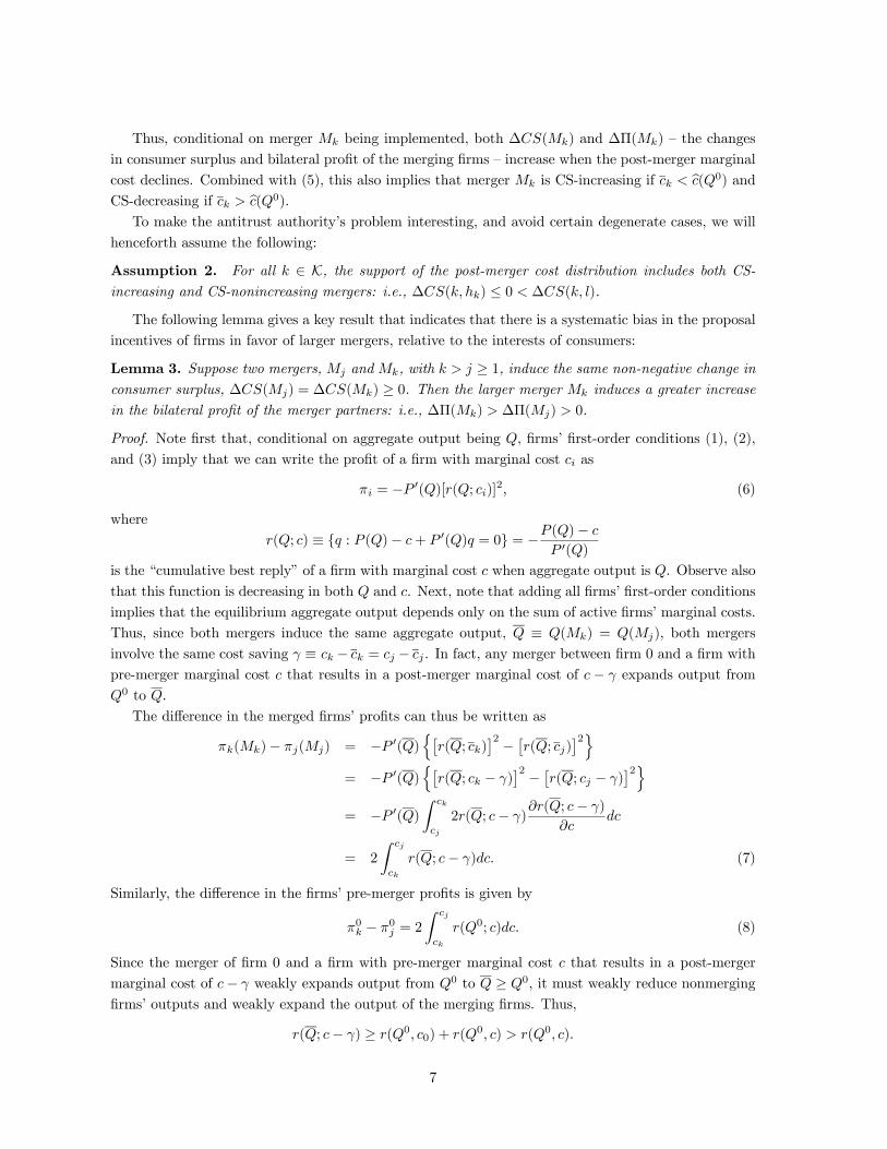
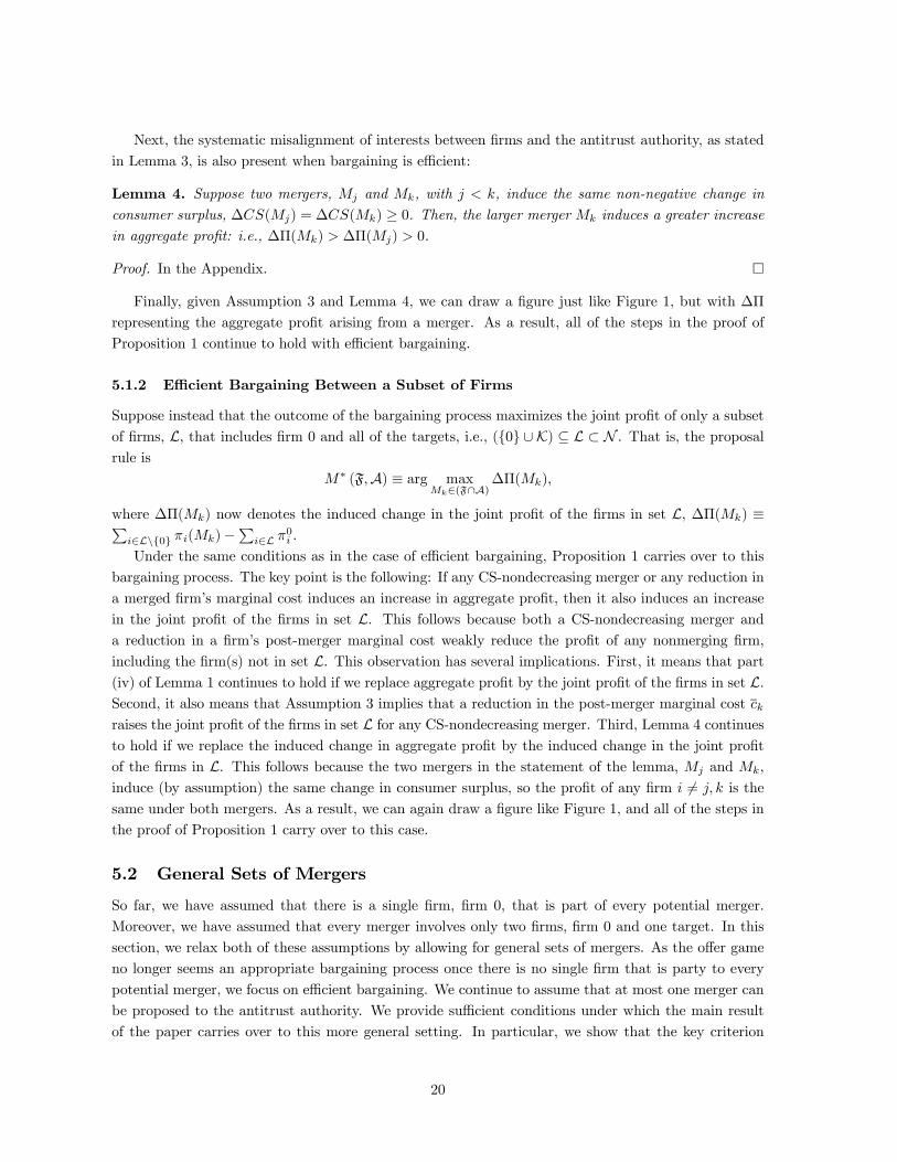
Figure 1: The curves depict the relationship between the change in consumer surplus and the change inbilateral profit of the various mergers, where each point on a curve corresponds to a different realizationof post-merger marginal cost for that merger.

By (7) and (8), this implies that πk(Mk)−πj(Mj) > π0k−π0j , which can be rewritten as ∆Π(Mk) >

∆Π(Mj).

Lemmas 1 to 3 imply that the possible mergers can be represented as shown in Figure 1 (wherethere are four possible mergers; i.e., K = 4). In the figure, the change in the merging firms’ bilateral

profit, ∆Π, is measured on the horizontal axis and the change in consumer surplus, ∆CS, is measuredon the vertical axis. The CS-increasing mergers therefore are those lying above the horizontal axis.The bilateral profit and consumer surplus changes induced by a merger between firms 0 and k ≥ 1,(∆Π(Mk),∆CS(Mk)), fall somewhere on the curve labeled “Mk.” (The figure shows only the parts ofthese curves for which the bilateral profit change ∆Π is nonnegative.) Since by Lemma 1 a CS-neutralmerger is profitable for the merger partners, each curve crosses the horizontal axis to the right of thevertical axis. By Lemma 2, the curve for each merger Mk, k ≥ 1, is upward sloping. By Lemma 3,on and above the horizontal axis the curves for larger mergers lie everywhere to the right of those forsmaller mergers.

A useful corollary of Lemmas 2 and 3, which can easily be seen in Figure 1, is the following:

Corollary 1. If two CS-nondecreasing mergers Mj and Mk with k > j ≥ 1 have ∆Π(Mk) ≤ ∆Π(Mj),

then ∆CS(Mk) < ∆CS(Mj).

Proof. Suppose instead that∆CS(Mk) ≥ ∆CS(Mj). Then there exists a c0k > ck such that∆CS(k, c0k) =

8

∆CS(Mj). But this implies (using Lemma 2 for the first inequality and Lemma 3 for the second) that∆Π(Mk) > ∆Π(k, c

0k) > ∆Π(Mj), a contradiction.

3.2 Main Result

We can now turn to the optimal policy of the antitrust authority. Recall that the antitrust authoritycan without loss restrict itself to approval sets in which the set of acceptable cost levels for a mergerbetween firm 0 and each firm k, Ak ⊆ [l, hk], is a union of closed intervals. Throughout we restrictattention to such policies.5 Let ak ≡ max{ck : ck ∈ Ak} denote the largest allowable post-merger costlevel for a merger (i.e., the “marginal merger”) between firms 0 and k. Also let ∆CSk ≡ ∆CS(k, ak)and ∆Πk ≡ ∆Π(k, ak) denote the changes in consumer surplus and bilateral profit, respectively,induced by that marginal merger. These are the lowest levels of consumer surplus and bilateral profitin any allowable merger between firms 0 and k.At first glance, one may be tempted to conjecture that the antitrust authority can achieve its goal

by simply approving any proposed merger that is CS-nondecreasing, i.e., for every k ≥ 1, setting

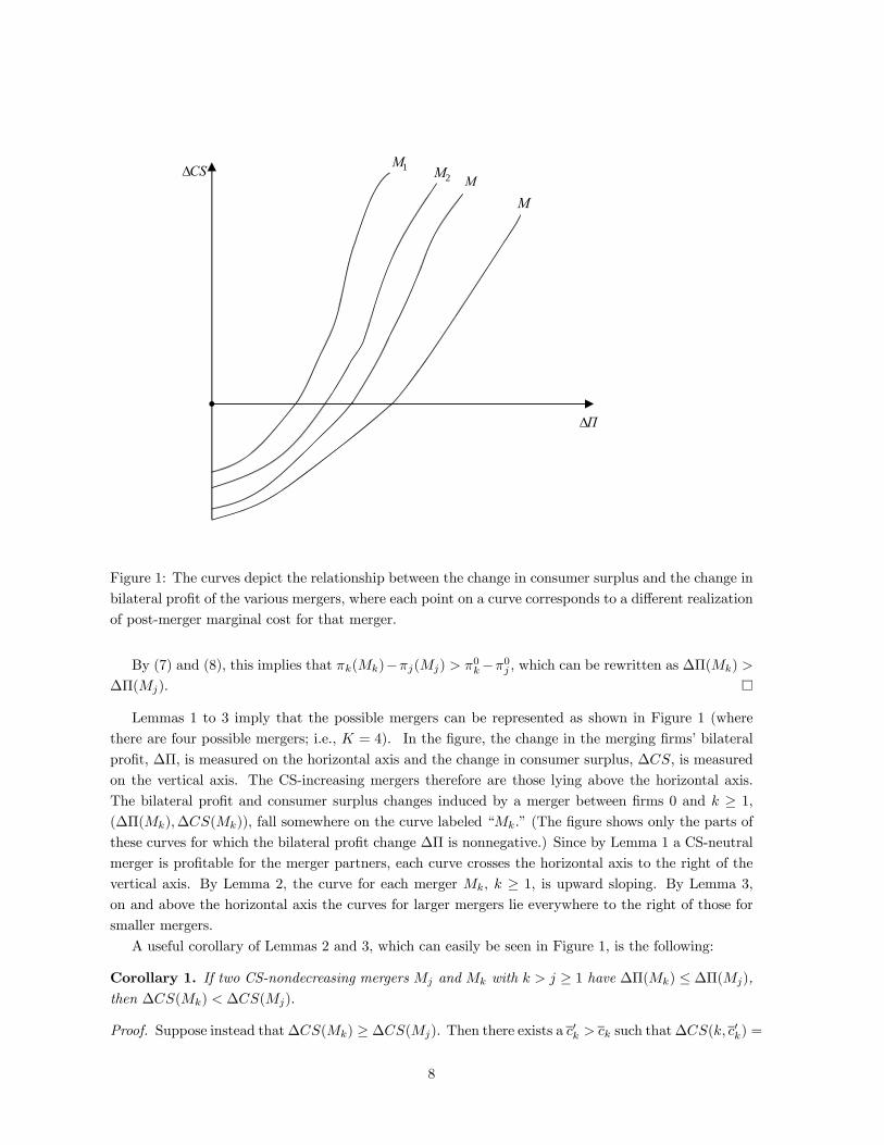
Ak = [l, ak], where ak is such that ∆CS(k, ak) = 0. Figure 2(a) illustrates such a policy for a case inwhich K = 4. In the figure, the approval set A is shown by the heavily-traced sections of the mergercurves. In fact, this is not an optimal policy. To see this, suppose the antitrust authority instead adoptsan approval policy A0 that imposes a slightly tougher standard on the largest merger: setting A0k = Ak

for each merger k 6= 4, and setting A04 = {M4 : ∆CS(M4) ≥ ε} for ε > 0 sufficiently small. Thisacceptance set is shown in Figure 2(b). The two policies differ only in the event that the most profitablefeasible and acceptable merger under approval policy A, M∗(F,A), lies in set A\A0, i.e., only whenM∗(F,A) = M4 and ∆CS(M4) ∈ [0, ε). Conditional on this event, the expected change in consumersurplus under approval policy A is bounded from above by ε, which approaches zero as ε becomes small.Under the alternative approval policy A0, and conditioning on the same event, the firms will proposethe next-most profitable acceptable merger (which must involve a target k < 4). Since the two policiesdo not differ in their acceptance sets for such smaller mergers, the expected change in consumer surplusunder A0 thus converges to EF [∆CS (M

∗(F\M4,A)) |∆Π (M∗(F\M4,A)) ≤ ∆Π4] > 0 as ε becomessmall. Hence, the expected change in consumer surplus is larger under A0 than under the naive approvalpolicy A.Since the naive policy of approving any CS-nondecreasing merger is not optimal, how should the

antitrust authority construct its approval policy to maximize expected consumer surplus? Our mainresult is the following:

Proposition 1. Any optimal approval policy A approves the smallest merger if and only if it is CS-nondecreasing, approves only mergers k ∈ K+ ≡ {1, ..., bK} with positive probability ( bK may equal K),and satisfies 0 = ∆CS1 < ∆CS2 < ... < ∆CSK for all k ≤ bK. That is, the lowest level of consumersurplus change that is acceptable to the antitrust authority equals zero for the smallest merger M1, isstrictly positive for every other merger Mk with k > 1, and is monotonically increasing in the size ofthe merger, while the largest merger(s) may never be approved.

According to Lemma 3, there is a systematic misalignment between firms’ proposal incentives andthe interests of the antitrust authority: firms tend to have an incentive to propose a merger that is

5Thus, when we state that any optimal policy must have a particular form, we mean any optimal interval policy ofthis sort. There are other optimal policies that add or subtract in addition some measure zero sets of mergers, since thesehave no effect on expected consumer surplus.

9

A′t Improvemen (b)

1M 2M MM

ΠΔ

CSΔ 1M 2M MM

ΠΔ

CSΔ

ε

ASet Approval Naive (a)

Figure 2: The “naive” policy that accepts all mergers that do not decrease consumer surplus is notoptimal. Here, requiring a strictly positive increase in consumer surplus to approve merger M4 raises

expected consumer surplus.

larger (in terms of the target’s pre-merger size) than the one that would maximize consumer surplus.Proposition 1 shows that to compensate for this intrinsic bias in firms’ proposal incentives, the antitrustauthority optimally adopts a higher minimum CS-standard the larger is the proposed merger. Here wegive a heuristic derivation of the result; see the formal proof in the Appendix for details. We organizeour discussion in “steps” corresponding to those in the formal proof in the Appendix.

Step 1. Observe, first, that the optimal policy A does not approve CS-decreasing mergers. That is,∆CSk ≥ 0 for all k ∈ K+, where K+ is the set of targets for whom the probability of having a mergerMk ∈ A is strictly positive. For any set A that does approve such mergers, the antitrust authoritycan increase the expected consumer surplus by instead adopting the alternative policy A+ that differsfrom A only in that it does not contain CS-decreasing mergers. In Figure 3, two such approval sets aredepicted in heavy trace. Now, in the event in which, under policy A, the most profitable feasible andallowable merger would have been CS-decreasing, ∆CS(M∗(F,A)) < 0, the merger that is proposedinstead under A+ is instead CS-nondecreasing. In any other event, the two policies induce the sameoutcome. Hence, the expected consumer surplus induced by policy A is lower than that induced by thealternative policy A+.Step 2. Next, note that every CS-nondecreasing smallest merger (M1) must be included in the

optimal approval set. If not, as in the set A shown in Figure 4(a), we could change the approval set Aby adding all CS-nondecreasing mergersM1, resulting in the alternative approval set A0 shown in Figure4(b). This change of approval sets matters only in the event in which, under A0, a CS-nondecreasingmerger M1 would be proposed and approved while, under A, this merger would not be approved andfirms would therefore propose the next-most profitable allowable merger (which may be the null merger

10

1M 2M MM

ΠΔ

CSΔ 1M 2M MM

ΠΔ

CSΔ

+ASet Approval (b)ASet Approval (a)

Figure 3: Changing the approval set A by blocking all mergers that reduce consumer surplus, resultingin approval set A+, raises expected consumer surplus.

M0). From Corollary 1, this next-most profitable allowable merger must increase consumer surplus byless than merger M1. Hence, expected consumer surplus is higher under the alternative approval setA0 than under A.Step 3. In any optimal approval set A, the consumer surplus level of the marginal merger Mk =

(k, ak), k ∈ K+, equals the expected CS-level of the next-most profitable acceptable merger, so that∆CSk = EAk (ak), as illustrated in Figure 5 for k = 2, where the expectation EA2 (a2) is the expected

level of ∆CS, conditional on the next-most-profitable merger being in the shaded region. To see thisindifference condition, suppose first that the consumer surplus level of the marginal merger Mk is lessthan the expected CS-level of the next-most profitable acceptable merger, i.e., ∆CSk < EAk (ak). Con-sider changing the approval set A by removing all mergersMk with ck ∈ (ak−ε, ak], thereby increasing∆CSk. For ε > 0 sufficiently small, this change in the approval set increases expected consumer sur-plus.6 Similarly, if ∆CSk > EA

k (ak), the antitrust authority can increase expected consumer surplusby adding to the approval set all mergers Mk ∈ (ak, ak + ε) for ε > 0 sufficiently small.7

Step 4. Next, we can see that any optimal approval policy A has the property that the increasein bilateral profit induced by a marginal merger is greater for larger mergers: ∆Πj ≤ ∆Πk for j < k,j, k ∈ K+. Panel (a) of Figure 6, where ∆Π2 > ∆Π3, depicts a situation where this property is not

satisfied. Intuitively, the merger cM2 directly above the marginal merger (3, a3), has a higher level of∆CS than does (3, a3), while resulting in the same expected ∆CS if it is rejected. Hence, if (3, a3)is approved, so should be cM2, or more precisely, so should those in the set A

ε

2 (for small ε) shown inFigure 6(b).

6Note that k ∈ K+ implies that ak > l, so that ak − ε > l for ε > 0 sufficiently small.7By Step 1 and Assumption 2, we have ak < hk, implying that ak + ε < hk for ε > 0 sufficiently small.

11

1M 2M MM

ΠΔ

CSΔ 1M 2M MM

ΠΔ

CSΔ

A ′Set Approval (b)ASet Approval (a)

Figure 4: Changing the approval set A by approving the smallest merger M1 whenever it does notreduce consumer surplus, resulting in approval set A0, raises expected consumer surplus.

Figure 5: The optimal approval policy is such that the increase in consumer surplus induced by themarginal merger Mk (shown here for k=2) equals the expected consumer surplus change from the

next-most-profitable acceptable merger, conditional on the marginal merger being the most profitablemerger in the set of feasible and acceptable mergers. The next-most-profitable acceptable merger musttherefore lie in the shaded region.

12

εjAA ΥSet Approval (b)ASet Approval (a)

1M 2M MM

ΠΔ

CSΔ

3CSΔ

2CSΔ

2ΠΔ3ΠΔ

2M̂

1M 2M MM

ΠΔ

CSΔ

3CSΔ

2CSΔ

2ΠΔ3ΠΔ

ε2A 2M̂

Figure 6: Panel (a) shows a situation where ∆Πk is not increasing in k; panel (b) shows an improvementin the approval set.

Step 5. Next, we can show that in any optimal approval policy A, the consumer surplus increaseinduced by the marginal merger is strictly greater for larger mergers, i.e., ∆CSj < ∆CSk for j < k,j, k ∈ K+. A situation in which this is not true is illustrated in Figure 7, where ∆CS2 ≥ ∆CS3. Bythe indifference condition of Step 3, ∆CS3 must equal the expected ∆CS of the next-most profitableallowable merger, i.e., ∆CS3 = EA3 (a3). Now, this expectation is the weighted average of the expected∆CS in two events. First, the next-most profitable allowable merger, say M 0, may be more profitable

than the marginal merger (2, a2), i.e., ∆Π(M 0) ∈ [∆Π2,∆Π3). In this event, M 0 must (by Step 4)involve a smaller target (either firm 1 or 2). Hence, the expected ∆CS in this event strictly exceeds∆CS2. Second, the next-most profitable acceptable mergerM

0 may be less profitable than the marginalmerger (2, a2), i.e., ∆Π(M 0) < ∆Π2. By the indifference condition of Step 4, the expected ∆CS in thisevent is exactly equal to ∆CS2. Taking the weighted average of these two events, we conclude that∆CS3 = EA3 (a3) > ∆CS2, a contradiction.Step 6. Finally, we argue that if there exists a merger Mj that will never be approved under the

optimal policy A, then no larger merger Mk, k > j, will ever be approved either: i.e., k /∈ K+ impliesk + 1 /∈ K+. To see this, observe that ∆CS(k, l) > ∆CS(k + 1, l) > ∆CS(k + 1, ak+1) [the firstinequality follows because the sum of costs after merger (k+1, l) is lower than that after merger (k, l),

whereas the second follows by Lemma 2], so as in Step 5, there is a nonmonotonicity in the ∆CS-levelsof the marginal mergers with firms k and k + 1: i.e., ∆CS(k, l) > ∆CS(k + 1, ak+1). The result thenfollows using an argument like that in Step 5; see the Appendix for details.

13

1M2M M

M

ΠΔ

CSΔ

3CSΔ2CSΔ

3ΠΔ

2ΠΔ

Figure 7: The optimal approval set is such that the consumer surplus increase induced by the marginalmerger Mj , is less than that by the marginal larger merger Mk, k > j, i.e., ∆CSj < ∆CSk. In thefigure, ∆CS2 > ∆CS3, which is a violation of that property.

4 Cutoff Policies and Comparative Statics

Proposition 1 shows that in any optimal policy the least efficient acceptable merger involving a target k

[the marginal mergerMk = (k, ak)] involves a larger increase in consumer surplus (and larger increase inbilateral profit) the larger is the target. Moreover, the result holds for any distributions of post-mergermarginal costs. However, it does not fully characterize those marginal mergers. Indeed, while we knowthat the marginal merger Mk = (k, ak) satisfies the indifference condition ∆CS(Mk) = EA

k (ak), theexpectation EAk (ak) depends on the acceptance sets for mergers other than k (i.e, on Aj , j 6= k), whoseoptimal forms depend in turn on merger k’s acceptance set Ak.Identifying the marginal merger for each target would be much simpler if we knew that the optimal

policy had a “cutoff” structure, in which, for each target k, any mergers with greater efficiencies thanthe marginal merger are accepted. Specifically, a cutoff policy AC is defined by a set of marginal costcutoffs, (aC1 , ..., a

CK), such that Mk = (k, ck) ∈ AC if and only if ck ≤ aCk . In that case, Proposition 1

would imply that the marginal mergers could be found by a simple recursive procedure: accept all CS-nondecreasing mergers M1 [i.e., set aC1 = bc1(Q0)], then for k = 2, ...,K recursively identify the largestpost-merger cost level aCk for which ∆CSk(k, aCk ) = EA

C

k (aCk ), where now the expectation EAC

k (aCk )

depends only on the already-determined cutoffs for mergers 1, ..., k − 1. If ∆CS(k, ck) < EAC

k (ck) forall ck ∈ [l, hk], then no such cutoff exists for merger Mk, so that AC

k = ∅. Moreover, this will alsoimply that AC

k0 = ∅ for all k0 > k.Unfortunately, however, as the following example illustrates, the optimal policy need not have a

cutoff structure. (For simplicity, the example considers a case where, contrary to the assumption of

14

ΠΔ

CSΔ

01.

04.

64.

05.

01.

0.9Prob=

0.1Prob=

1M

2M

05.

),2( 2c′

),2( 2c ′′

Figure 8: The figure depicts an example where the optimal approval set does not have a cutoff structure.

the model, one of the mergers has a finite support of post-merger marginal costs. But the same insightwould obtain if we perturbed the example and assumed that the support is continuous with no atoms.)

Example 1. Suppose that there are two possible mergers, M1 and M2 . The smaller merger, M1,is always feasible. Its post-merger marginal cost is either c1 = l or c1 = h1, where the probabilityon the latter is 0.9. The corresponding changes in consumer surplus and bilateral profit are givenby (∆Π(1, l),∆CS(1, l)) = (5, 5) and (∆Π(1, h1),∆CS(1, h1)) = (1, 1). The unconditional expectedincrease in consumer surplus from approving M1 is thus equal to 4.6. The post-merger marginal costof the larger merger, M2, has a continuous support [l, h2] with no atoms, satisfying ∆CS(2, h2) <1 and ∆CS(2, l) > 5. Let c02 be such that ∆CS(2, c

02) = 4.6 and c002 be such that ∆Π(2, c

002) = 5, and

assume that c02 < c002 . It is straightforward to verify that, in this case, the optimal approval policyA∗ is such that A∗1 = {l, h1} and A∗2 = [l, c02] ∪ [c002 , a2]. This situation is illustrated in Figure 8.To see why the optimal approval policy for M2 does not have a cut-off structure, note that for anypost-merger marginal cost c2 ∈ (c02, c002), M2 would always be the proposed merger if it were approvedwhen proposed. But the induced change in consumer surplus from M2 would be less than 4.6, which isthe expected change in consumer surplus from M1. The optimal policy corrects for this bias in firms’proposal policies by rejecting merger M2 whenever c2 ∈ (c02, c002).

15

Nonetheless, our next result provides a sufficient condition that ensures that the recursively-definedcutoff policy is in fact optimal. To proceed, let AC(J) ⊆ Πk∈J [l, hk] denote the recursively-definedcutoff policy when only mergers with targets in set J are possible; that is, when we suppose that thereis no possibility for a merger with any target k /∈ J . [The policy AC(J) specifies #J cutoffs.] Forconvenience, when J = K we write AC ≡ AC(K). We also let aCk (J) denote the cutoff level of marginalcost for a merger with target k in cutoff policy AC(J).In addition, for a set of targets J ⊆ K, define the realized set of feasible mergers to be FJ , and the

functionECS(∆Π;A, J) ≡ EFJ [∆CS(M

∗(FJ ,A))|∆Π(M∗(FJ ,A)) ≤∆Π]

as the expected value of ∆CS under policy A ⊆ Πk∈J [l, hk] from the most profitable acceptable mergerinvolving targets in set J , conditional on that merger’s increase in bilateral profit being no greaterthan ∆Π.8 Note that the structure of A at profit levels above ∆Π affects the value of this conditionalexpectation by changing the conditional distributions of post-merger marginal costs. Specifically, theprobability of a merger in setMj ⊆ {Mj : ∆Π(Mj) ≤ ∆Π} being feasible conditional on the most prof-itable acceptable merger having a profit level below ∆Π is Pr(Mj ∈Mj)× [1− Pr(∆Π(Mj) > ∆Π andMj ∈ Aj)]

−1. Note that an optimal policyA∗ ⊆ Πk∈K[l, hk] is an element of argmaxAECS(∞;A,K).We then have:

Proposition 2. Suppose that for every J ⊆ K with 1 ∈ J the following property holds:9

Every merger Mk = (k, ck) ∈ AC(J) with ck < aCk (J) has ∆CS(Mk) > ECS(∆Π(Mk);AC(J\k), J\k).(9)

Then, the cutoff policy AC is an optimal policy.

Proof. In the Appendix.

While Proposition 2 does not offer a condition on primitives, it allows us to verify that therecursively-derived cutoff policy is optimal. The following example provides an illustration of itsuse.

Example 2. Consider a four-firm industry (so N = 4) in which firm 0 can merge with each of theother firms (so K = 3). Industry inverse demand is P (Q) = 1 − Q. Pre-merger marginal costsare c0 = c2 = 0.5, c1 = 0.55, and c3 = 0.45, so the pre-merger market shares are s0 = s2 = 1/4,s1 = 1/8, and s4 = 3/8. The naive policy marginal cost cutoffs (where any CS-nondecreasing mergeris accepted) are a1 = 0.45, a2 = 0.40, a3 = 0.35. Now suppose that each merger has a 3/4 probabilityof being feasible (so θk = 0.75 for k = 1, 2, 3) and that, conditional on being feasible, the post-mergermarginal cost is distributed with a beta distribution between the merger’s naive cutoff and 0.2.10 Whenβ = 1 and α = 5, expected consumer surplus could be increased by 6.44% if there were there noinformational asymmetry between the firms and the antitrust authority (so the merger that increased

8Thus, EAk (ck) = ECS(∆Π(k, ck);AK\k,K\k) where AK\k ≡ Πj∈K\kAj .9Note that property (9) necessarily holds for j = 1; the assumption made here is that it holds for all j > 1.10One can think of this situation as having a 1/4 probability of there being no CS-increasing merger, and a 3/4

probability of a CS-increasing merger. The beta distribution has a pdf f(x|α, β) that is proportional to xα−1(1− x)β−1.Its mean is the lower bound of its support plus a fraction α/(α + β) of the difference between its support’s upper andlower bounds. When β = 1 and α > 1, as in the cases we study here, the pdf is an increasing function, so that smallefficiency gains are more likely than large ones. The lower bound of 0.2 is chosen to ensure that all firms remain activeafter any merger.

16

consumer surplus most would always be implemented). In this setting, one can verify that the sufficientcondition of Proposition 2 is satisfied, so the recursively-defined cutoff policy is optimal. The cutoffsin this optimal policy are a1 = 0.45, a2 = 0.383, and a3 = 0.316, with associated changes in consumersurplus of ∆CS1 = 0, ∆CS2 = .00170, and ∆CS3 = .00346. The optimal policy achieves 90.30%of the first-best increase in expected consumer surplus, while the naive policy achieves 79.83% of this

amount. This outcome is shown in Table 1. The table also shows the results when α = 3 and α = 1

(α = 1 is a uniform distribution). Both of these cases also satisfy the sufficient condition in Proposition2. As α decreases, the distributions of post-merger marginal costs (conditional on the merger beingfeasible) shift towards lower costs and the expected consumer surplus gain increases. However, the gainfrom the fully optimal policy relative to the naive policy falls.

Table 1:

α CS1 CS2 CS3first-best:

% gain in E[CS]

naive policy:% of first-best gain

optimal policy:% of first-best gain

5 0 0.00170 0.00346 6.44 79.83 90.30

3 0 0.00170 0.00457 9.55 87.34 92.13

1 0 0.00099 0.00571 18.15 93.67 94.10

4.1 Comparative Statics

When cutoff rules are optimal we can explore how changes in underlying parameters alter the natureof the optimal policy. We provide two such results here, assuming that the optimal policy has acutoff structure. Consider, first, changes in the feasibility probabilities. Intuitively, lower feasibilityprobabilities should move the optimal policy toward the naive one. For example, as all θ’s approach

zero, the optimal policy approaches the naive policy, since there is almost no chance that two mergersare feasible. Our first result, which builds on this intuition, examines the effect of a decrease in thelikelihood that a merger with a given target k is feasible.

Proposition 3. Consider an decrease in the probability of merger Mk’s feasibility from θk to θ0k < θk,

assuming that Mk is initially approved with positive probability (i.e., k ≤ bK). Then, under the optimalmerger approval policy, ∆CSj

0 = ∆CSj for any weakly smaller merger Mj, j ≤ k, and ∆CS0j < ∆CSjfor any larger merger Mj, j > k, that is approved with positive probability.

Proof. In the Appendix.

Our second result concerns a change in pre-merger costs:

Proposition 4. Consider a reduction in firm 0’s marginal cost from c0 to c00 < c0. Under the optimalmerger approval policy, this induces a decrease in all post-merger marginal cost cutoffs: a0k < ak forevery 1 ≤ k ≤ bK.Proof. In the Appendix.

5 Extensions

In this section, we consider five extensions of our baseline model. First, we consider alternative bargain-ing processes among firms. Second, we analyze the optimal merger approval policy in a more general

17

setting by relaxing two assumptions: (i) every merger involves two firms, and (ii) firm 0 is party to anymerger. Third, adopting an aggregative game approach, we consider the case of price competition withdifferentiated products (CES and multinomial logit demand structures). Fourth, we study the optimalmerger approval policy when the antitrust authority cares not only about consumer surplus but alsoabout producer surplus. Finally, we extend the model by allowing for synergies in fixed costs.

5.1 Other Bargaining Processes

In our analysis so far, we have focused on the case where the bargaining process between firms is givenby the offer game [Segal (1999)]. In the offer game, firm 0 makes a take-it-or-leave-it offer to a targetof its choosing and is therefore able to extract all of the gain in bilateral profit. The equilibrium of theoffer game therefore results in the proposal of the merger that maximizes the change in the bilateralprofit of the merger partners in the realized set of feasible and acceptable mergers.

It is straightforward to see that the same outcome would obtain if the bargaining power were moreevenly distributed between firms, provided firm 0 can extract the same fixed fraction of the gain inbilateral profit with each target. This would hold, for example, if firm 0 first selects a potential target,say firm k, and then the bargaining process between firm 0 and firm k is given by the alternatingoffer bargaining game of Rubinstein (1982), assuming that all potential targets have the same discountfactor.In the following, we explore two alternative bargaining processes. First, we consider the benchmark

case of efficient bargaining. Second, we consider the case where there is efficient bargaining only amonga subset of firms (including all of the firms that are involved in potential mergers). We show that, inboth cases, our main result continues to hold: the optimal approval policy has the property that the

minimum CS-standard is increasing in the size of the proposed merger.

5.1.1 Efficient Bargaining

Suppose the outcome of the bargaining process is efficient for the firms in the industry in the sense thatit maximizes aggregate profit. That is, we assume that, from the realized set of feasible and acceptablemergers, F ∩A, firms choose to propose merger

M∗ (F,A) ≡ arg maxMk∈(F∩A)

∆Π(Mk),

where ∆Π(Mk) now denotes the change in aggregate profit induced by merger Mk,

∆Π(Mk) ≡X

i∈N\{0}πi(Mk)−

Xi∈N

π0i .

There are several bargaining processes that would lead to aggregate profit maximization:

1. “Coasian bargaining” among all firms under complete information.

2. A “menu auction” in which each firm i 6= 0 submits a nonnegative bid bi(Mk) ≥ 0 to firm 0 foreach merger Mk ∈ (F ∩A), k ≥ 1, and firm 0 then selects the merger that maximizes its profit,

inclusive of these bids. [Firm 0’s profit from selecting the null merger M0 is π0(M0).] Bernheimand Whinston (1996) show that there is an efficient equilibrium which, in this setting, implementsthe merger that maximizes aggregate profit.

18

3. The target (firm 0) committing to a sales mechanism. Jehiel, Moldovanu, and Stacchetti (1996)show that an optimal mechanism has the following structure in our setting: Firm 0 proposes to im-plement the aggregate profit-maximizing mergerM∗ (F,A) and requires the payment πi(M∗ (F,A))−πi(M i) from each firm i 6= 0, where M i is the merger in set (F ∩A) \Mi that minimizes firm i’sprofit. If a firm i does not accept participation in the mechanism when all other firms do, then the

principal commits to proposing merger M i to the antitrust authority.11 Given this mechanism,

there is an equilibrium in which all firms participate in the mechanism, and merger M∗ (F,A) isproposed.12

We claim that Proposition 1 continues to hold when bargaining is efficient. The key steps in theargument are the following: First, note that Lemma 1 states that a CS-neutral mergerMk, k ≥ 1, raisesnot only the bilateral profit of the merger partners but also aggregate profit, i.e., that ∆Π(Mk) > 0.Lemma 2, however, does not extend to the case of aggregate profit without imposing an additional

condition. We therefore assume that a reduction in post-merger marginal cost increases aggregate profitif the merger is CS-nondecreasing:

Assumption 3. If merger Mk, k ≥ 2, is CS-nondecreasing [i.e., if ck ≤ bc(Q0)], then reducing itspost-merger marginal cost ck increases the aggregate profit

Pi∈N\{0} πi(Mk).13

In fact, this assumption must hold for merger Mk if pre-merger cost differences are small enoughso that the sum of the pre-merger market share of firms 0 and k weakly exceeds the pre-merger shareof any other firm, i.e., s00 + s0k ≥ maxj 6=0,k s0j .14 To see why Assumption 3 holds in this case, note thatsumming up the first-order conditions for profit maximization following merger Mk [conditions (2) and(3)] yields X

i∈N\{0}πi(Mk) =

Xi∈N\{0,k}

[P (Q(Mk))− ci] qi(Mk) + [P (Q(Mk))− ck] qk(Mk)

=¯̄̄[Q(Mk)]

2 P 0(Q(Mk))¯̄̄H(Mk), (10)

where H(Mk) ≡P

i∈N\{0}(si(Mk))2 is the post-merger industry Herfindahl index. Assumption 1

ensures that the first term,¯̄Q2P 0(Q)

¯̄, is increasing in Q. By Lemma 2, a reduction in post-merger

marginal cost ck leads to a larger Q(Mk), so a sufficient condition for the claim to hold is that reducingthe merged firm’s marginal cost ck induces an increase in H(Mk). Under Assumption 1, a decreasein the merged firm’s marginal cost ck increases the share of the merged firm and decreases the share

of every other firm. Since s00 + s0k ≥ maxj 6=0,k s0j implies sk(Mk) ≥ maxj 6=0,k sj(Mk) for any CS-

nondecreasing merger Mk with k ∈ {1, ...,K}, this induced change in market shares increases thepost-merger Herfindahl index H(Mk) (see Lemma 7 in the Appendix).

11 Similar to Bernheim and Whinston’s (1996) menu auction, firms i 6= 0 make payments even when they are not partyto a merger.12To see that firm 0 wants to propose merger M∗ (F,A), note that using this type of mechanism its optimal merger

proposal solvesmax

Mk∈(F∩A)Π(Mk)−

i 6=0πi(Mi),

which is equivalent to maxMk∈(F∩A)Π(Mk).13Note that we make this assumption only for mergers with targets k ≥ 2 because the arguments in Proposition 1 rely

on monotonicity of the merger curves only for mergers other than the smallest merger.14 In Section 5.2, where we consider more general sets of mergers, we provide a weaker sufficient condition for Assumption

3 to hold.

19

Next, the systematic misalignment of interests between firms and the antitrust authority, as statedin Lemma 3, is also present when bargaining is efficient:

Lemma 4. Suppose two mergers, Mj and Mk, with j < k, induce the same non-negative change inconsumer surplus, ∆CS(Mj) = ∆CS(Mk) ≥ 0. Then, the larger merger Mk induces a greater increasein aggregate profit: i.e., ∆Π(Mk) > ∆Π(Mj) > 0.

Proof. In the Appendix.

Finally, given Assumption 3 and Lemma 4, we can draw a figure just like Figure 1, but with ∆Πrepresenting the aggregate profit arising from a merger. As a result, all of the steps in the proof ofProposition 1 continue to hold with efficient bargaining.

5.1.2 Efficient Bargaining Between a Subset of Firms

Suppose instead that the outcome of the bargaining process maximizes the joint profit of only a subsetof firms, L, that includes firm 0 and all of the targets, i.e., ({0} ∪K) ⊆ L ⊂ N . That is, the proposalrule is

M∗ (F,A) ≡ arg maxMk∈(F∩A)

∆Π(Mk),

where ∆Π(Mk) now denotes the induced change in the joint profit of the firms in set L, ∆Π(Mk) ≡Pi∈L\{0} πi(Mk)−

Pi∈L π

0i .

Under the same conditions as in the case of efficient bargaining, Proposition 1 carries over to thisbargaining process. The key point is the following: If any CS-nondecreasing merger or any reduction ina merged firm’s marginal cost induces an increase in aggregate profit, then it also induces an increasein the joint profit of the firms in set L. This follows because both a CS-nondecreasing merger anda reduction in a firm’s post-merger marginal cost weakly reduce the profit of any nonmerging firm,including the firm(s) not in set L. This observation has several implications. First, it means that part(iv) of Lemma 1 continues to hold if we replace aggregate profit by the joint profit of the firms in set L.Second, it also means that Assumption 3 implies that a reduction in the post-merger marginal cost ckraises the joint profit of the firms in set L for any CS-nondecreasing merger. Third, Lemma 4 continuesto hold if we replace the induced change in aggregate profit by the induced change in the joint profitof the firms in L. This follows because the two mergers in the statement of the lemma, Mj and Mk,induce (by assumption) the same change in consumer surplus, so the profit of any firm i 6= j, k is thesame under both mergers. As a result, we can again draw a figure like Figure 1, and all of the steps inthe proof of Proposition 1 carry over to this case.

5.2 General Sets of Mergers

So far, we have assumed that there is a single firm, firm 0, that is part of every potential merger.Moreover, we have assumed that every merger involves only two firms, firm 0 and one target. In thissection, we relax both of these assumptions by allowing for general sets of mergers. As the offer gameno longer seems an appropriate bargaining process once there is no single firm that is party to everypotential merger, we focus on efficient bargaining. We continue to assume that at most one merger canbe proposed to the antitrust authority. We provide sufficient conditions under which the main resultof the paper carries over to this more general setting. In particular, we show that the key criterion

20

according to which the antitrust authority should optimally discriminate between alternative mergersis the naively-computed post-merger Herfindahl index. This naively-computed post-merger index isfrequently used by antitrust authorities in merger analysis as it is entirely based on readily availableinformation on pre-merger market structure.To proceed, let mk ≥ 2 denote the number of merger partners in merger Mk and let cMk

denote the

realized post-merger marginal cost of merger Mk. It is straightforward to see that the characterizationof CS-neutral mergers in Lemma 1 extends to any mk ≥ 2. In particular, any CS-neutral mergerraises aggregate profit. In Section 5.1, we have shown that aggregate profit following merger Mk isproportional to the post-merger Herfindahl index H(Mk), where the proportionality factor dependsonly on the post-merger aggregate output Q(Mk) [see (10)]. Observe that for a CS-neutral mergerMk,Lemma 1 implies that the actual post-merger Herfindahl index equals the naively-computed index:

H(Mk) ≡ [sk(Mk)]2 +

Xi/∈Mk

[si(Mk)]2

=

"Xi∈Mk

s0i

#2+Xi/∈Mk

£s0i¤2 ≡ Hnaive(Mk).

Thus, for any two CS-neutral mergers Mj and Mk, regardless of the number of merger partners, themerger that induces a greater naively-computed post-merger Herfindahl index also induces a greaterincrease in aggregate profit:

Hnaive(Mk) > Hnaive(Mj)⇔ ∆Π(Mk) > ∆Π(Mj).

Hence, provided that merger curves slope upward in the positive orthant of (∆Π,∆CS)-space and donot intersect, Proposition 1 carries over to this more general setting, where a “larger” merger now refersto a merger that induces a greater increase in the naively-computed post-merger Herfindahl index.Under what conditions do the curves for CS-nondecreasing mergers slope upward and not intersect?

To identify such conditions, we first observe that the inverse of the slope of the curve for merger Mk

in (∆Π,∆CS)-space is given by (see Lemma 8 in the Appendix)

d∆Π(Mk)

d∆CS(Mk)= −2−

∙P 00(Q(Mk))Q(Mk)

P 0(Q(Mk))

¸H(Mk) +

∙2

P 0(Q(Mk))Q(Mk)

¸ ∙r(Q(Mk); cMk

)

dQ(Mk)/dcMk

¸, (11)

where r(Q; c) is again the cumulative best reply of a firm with marginal cost c to aggregate output Q.We now use expression (11) to identify condtions under which the merger curves are upward-sloping

and non-intersecting.15 As earlier, merger curves are upward-sloping in the positive orthant wheneverthe pre-merger joint market share of any merging firms exceed the pre-merger share of the largestnonmerging firm. However, expression (11) allows us to derive a weaker condition than this:16

15Condition (11) also offers an alternative method to establish Lemma 4. To see this, observe that, in our baselinemodel, if two mergers induce the same change in consumer surplus, ∆CS, and the same change in aggregate profit, ∆Π,then the two mergers also induce the same aggregate output Q and the same post-merger Herfindahl index H. Moreover,in our baseline model, the firm resulting from a larger merger has a larger output r(Q; cM ) (as it faces a larger i6=M ci,and so must have a lower cM if it induces an equal CS-level). Hence, (11) implies in that model that if there were a pointof intersection, the curve of the larger merger would have a larger value of d∆Π/d∆CS, hence a flatter curve, whichyields a contradiction since the larger merger’s curve must cross from below at the first crossing since the larger merger’scurve lies further to the right where ∆CS = 0.16That condition (12) below holds when snaiveMk

≥ maxi/∈Mks0i follows from the facts that in this case Hnaive(Mk) ≤

snaiveMkand (N −mk + 2)s

naiveMk

≥ 1. (Note that, in general, the Herfindahl index is bounded above by the share of thelargest firm.)

21

Lemma 5. The merger curve of merger Mk slopes upward in the positive orthant of (∆Π,∆CS)-spaceif the merged firm’s naively-computed post-merger market share snaiveMk

≡P

i∈Mks0i and the naively-

computed post-merger Herfindahl index Hnaive(Mk) satisfy

snaiveMk≥ Hnaive(Mk)

2≥ 1− (N −mk + 2)s

naiveMk

, (12)

where N + 1 is the pre-merger number of firms (and thus N −mk + 2 is the number of firms followingmerger Mk).

Proof. In the Appendix.

Now consider when the merger curves are non-intersecting. We will use expression (11) to provideconditions under which two merger curves cannot cross; that is, their ranking must be the same astheir ranking where ∆CS = 0. We will show this by contradiction, showing that the curve furtherto the right at ∆CS = 0 must have a smaller slope wherever the two curves cross. Since aggregateprofit and consumer surplus are the same wherever the curves cross, so must be the industry Herfindahl

index and aggregate quantity. By (11), this means the slopes at that point are ordered by the val-ues of r(Q(Mk); cMk)/(dQ(Mk)/dcMk). The following lemma provides a condition under which thosequantities are ordered in the correct way to give us an analog of Lemma 3:

Lemma 6. Consider two mergers Mj and Mk, with mj ≥ mk. If the firms in Mk jointly produce morepre-merger than the firms in Mj (i.e.,

Pi∈Mk

s0i >P

i∈Mjs0i ) and if the naively-computed post-merger

Herfindahl index is larger when Mk is implemented than when Mj is implemented [i.e., Hnaive(Mk) >

Hnaive(Mj)], then the curve relating to merger Mk lies to the right of that relating to merger Mj inthe positive orthant of (∆Π,∆CS)-space.

Proof. In the Appendix.

Finally, if all mergers have the same minimum of the support of post-merger marginal costs, denotedl, the maximum CS-increase that the smaller merger can achieve is larger than that of the largermerger.17 Hence, under the assumptions of Lemmas 5 and 6, the merger curves have all of the propertiesrequired to obtain our main result, the analog of Proposition 1.For example, one special case in which this result can be applied arises where there are three

potential mergers, one involving firms 1 and 2, a second involving firms 1 and 3, and a third involvingfirms 2 and 3. As before, the three mergers are mutually exclusive but, in contrast to the baselinemodel, there is no longer a single firm that is party to every potential merger. In this case, the twoconditions of Lemma 6 are satisfied if the mergers have the same ranking by both the product and thesum of the merging firms’ pre-merger market shares.

17To see this, consider a larger merger Mk and a smaller merger Mj , j < k. The maximum ∆CS induced by thelarger merger Mk is ∆CS(k, l). The assumption in Lemma 6 that the firms in Mk produce more pre-merger implies thatΣi∈Mk

ci < Σi∈Mjci. Since agrgegate quantity depends only on the sum of firms’ costs, this in turn implies that if the

two mergers induce the same change in consumer surplus, then cMk< cMj

. Thus, ∆CS(k, l) = ∆CS(j, cMj) implies

that cMj> l. Since ∆CS(j, cMj

) is decreasing in cMj, the maximum CS-increase for the smaller merger, ∆CS(j, l),

must be larger than that of the larger merger: i.e., ∆CS(j, l) > ∆CS(k, l).

22

5.3 Differentiated Products

In our analysis we have assumed that firms produce a homogeneous good and compete in a Cournotfashion. Restricting attention to the case of efficient bargaining between firms and mergers between

firm 0 and a single target firm k ∈ K, we now show that our main insights carry over to the case wherefirms compete in prices and produce symmetrically differentiated goods with consumers having CES ormultinomial logit demand. Specifically, we assume that the initial market structure is such that everyfirm produces one differentiated good. If a merger Mk is proposed and approved, then a merged firmproduces the two products of its merger partners at an identical post-merger marginal costs, ck.CES Demand. In the CES model, the utility function of the representative consumer is given by

U =

ÃNXi=0

Xρi

!1/ρZα,

where ρ ∈ (0, 1) and α > 0 are parameters, Xi is consumption of differentiated good i, and Z is

consumption of the numeraire. Utility maximization implies that the representative consumer spendsa constant fraction 1/(1+α) of his income Y on the N +1 differentiated goods (and the remainder onthe numeraire). Using the normalization Y/(1+α) ≡ 1, the resulting demand for differentiated good i

is

Xi =p−λ−1iPNj=0 p

−λj

,

where pi is the price of good i, and λ ≡ ρ/(1− ρ). The consumer’s indirect utility can be written as

V = (1 + α) lnY +1

λln

⎛⎝ NXj=0

p−λj

⎞⎠ . (13)

Multinomial Logit Demand. In the multinomial logit model, expected demand for product i isgiven by

Xi =exp

³a−piμ

´PN

j=0 exp³a−pjμ

´ ,where a > 0 and μ > 0 are parameters, and pj the price of product j. Letting Y denote income, theindirect utility of the representative consumer can be written as

V = Y + μ ln

⎡⎣ NXj=0

exp

µa− pjμ

¶⎤⎦ . (14)

The CES and multinomial logit models share important features with the Cournot model. Inparticular, all of these models can be written as “aggregative games.” That is, the profit a firm obtainsfrom its plant or product i can be written as

π(ψi, ci;Ψ),

where ψi ≥ 0 is the firm’s strategic variable, ci is its (constant) marginal cost, and Ψ ≡P

j ψj is anaggregator summarizing the “aggregate outcome.” [If a merged firm runs two plants or produces two

23

products at the same marginal cost ck and chooses the same value ψk of its strategic variable for both ofits plants or products, then its total profit is 2π(ψk, ck;Ψ).] Further, consumer surplus is an increasingfunction of the aggregator, and does not depend on its composition, so that it can be written as V (Ψ).In the Cournot model, ψi is output qi and Ψ is aggregate output Q, so that profit can be written as

π(ψi, ci;Ψ) = (P (Ψ)− ci)ψi and consumer surplus as V (Ψ) =R Ψ0(P (x)−P (Ψ))dx. In the CES model,

we have ψi = p−λi and Ψ =P

j p−λj , so that profit from product i can be written as

π(ψi, ci;Ψ) = [ψ−1/λi − ci]

ψ(λ+1)/λi

Ψ.

From the indirect utility (13), it follows that consumer surplus is an increasing function of Ψ. Finally,in the multinomial logit model, we have ψi = exp ((a− pi)/μ) and Ψ =

Pj exp ((a− pj)/μ), so that

profit from product i can be written as

π(ψi, ci;Ψ) = [a− μ lnψi − ci]ψiΨ.

From the indirect utility (14), it follows that consumer surplus is an increasing function of Ψ.In the Appendix, we show that the equilibrium profit functions of these three models share some

important properties. Using this common structure, we show in the Appendix that if merger Mk isCS-neutral, then it raises the joint profit of the merging firms as well as aggregate profit. Moreover,a reduction in post-merger marginal cost increases the merged firm’s profit and, provided pre-mergerdifferences between firms are not too large, aggregate profit. Moreover, if any two mergersMj andMk,k > j, induce the same nonnegative change in consumer surplus, then the larger merger Mk inducesa greater increase in aggregate profit than the smaller merger Mj . In sum, in the two differentiatedgoods models, the merger curves have the same features in (∆CS,∆Π)-space as in the Cournot model.

Our main result, Proposition 1, therefore carries over as well.

5.4 Alternative Welfare Standard

In our baseline model, we have assumed that the antitrust authority seeks to maximize consumersurplus. While this is in line with the legal standard in the U.S., the EU, and many other countries,it might seem unsatisfactory that the antitrust authority completely ignores any effect of its policy onproducer surplus. We now show that our main result extends to the case where the antitrust authorityseeks to maximize any convex combination of consumer surplus and aggregate surplus. We focus onthe case of efficient bargaining between firms, but discuss the offer game at the end of the section.Specifically, suppose the antitrust authority’s welfare criterion is W ≡ CS + λΠ, where λ ∈ [0, 1].

When λ = 1, welfare W thus amounts to aggregate surplus. Let

∆W (Mk) ≡ ∆CS(Mk) + λ∆Π(Mk)

denote the change in welfare induced by approving merger Mk. We will say that merger Mk is W-

increasing [resp. W-decreasing] if ∆W (Mk) > 0 [resp. ∆W (Mk) < 0]. It is W-nondecreasing [resp.W-nonincreasing] if ∆W (Mk) ≥ 0 [resp. ∆W (Mk) ≤ 0].Since a W-increasing merger may be CS-decreasing, we require a slightly stronger version of As-

sumption 3:

Assumption 3’ If merger Mk for k ≥ 2 is W-nondecreasing, then (i) reducing its post-merger mar-ginal cost ck increases the aggregate profit, and (ii) ck < min{c0, ck}; i.e., the merger involvessynergies.

24

Assumption 3’ must hold if pre-merger marginal cost differences are sufficiently small. To seethis, consider the extreme case where all firms have the same pre-merger marginal cost c. Then, formerger Mk to be W-nondecreasing, it must involve synergies in that ck < c.18 Hence, if Mk is W-nondecreasing, the merged firm is the firm with the lowest marginal cost post merger. Reducing themerged firm’s marginal cost ck therefore increases aggregate output Q (thereby raising |Q2P 0(Q)|) andthe Herfindahl index H. From equation (10), a lower level of post-merger marginal cost ck thus resultsin a greater aggregate profit. By continuity of consumer and producer surplus in marginal costs, itfollows that if pre-merger marginal cost differences are sufficiently small, then ∆W (Mk) ≥ 0 impliesthat ck < min{c0, ck} and aggregate profit is decreasing in ck .We also impose the following analog of Assumption 2:

Assumption 2’ For all k ∈ K, the support of the post-merger cost distribution includes both W-increasing and W-nonincreasing mergers: i.e., ∆W (k, hk) ≤ 0 < ∆W (k, l).

Assumption 3’ allows us to obtain a slightly stronger version of Lemma 4:

Lemma 4’ Suppose two W-nondecreasing mergers, Mj and Mk, with k > j ≥ 1, induce the samechange in consumer surplus, ∆CS(Mj) = ∆CS(Mk). Then the larger merger Mk induces agreater increase in aggregate profit: i.e., ∆Π(Mk) > ∆Π(Mj) > 0.

Proof. In the Appendix.

Figure 9(a) depicts the merger curves in (∆Π,∆CS)-space. The downward-sloping lines are isow-elfare curves, each with slope −λ; the dashed line is the isowelfare curve corresponding to no welfarechange, ∆W = 0. Lemma 4’ states that, above the dashed line ∆W = 0, the curve corresponding to alarger merger lies everywhere to the right of that corresponding to a smaller merger.Figure 9(b) depicts the merger curves in (∆Π,∆W )-space. Note that each merger curve has a

positive horizontal intercept: since a CS-nondecreasing merger increases aggregate profit, a W-neutralmerger must be CS-decreasing and therefore increase aggregate profit. Moreover, each curve is upward-

sloping in the positive orthant. Finally, in the positive orthant, the curve of a larger merger lieseverywhere to the right of that of a smaller merger.Letting∆W k ≡ ∆W (k, ak) denote the welfare level of the “marginal merger,” i.e., the lowest welfare

level in any allowable merger between firms 0 and k, we can then establish the following analog of ourmain result (Proposition 1) for the case in which the antitrust authority maximizes an arbitrary convexcombination of consumer surplus and aggregate surplus:

Proposition 1’ Any optimal approval policy A approves the smallest merger if and only if it is W-nondecreasing, and satisfies 0 = ∆W 1 < ∆W j < ∆W k for all j, k ∈ K+, 1 < j < k, whereK+ ⊆ K is the set of mergers that is approved with positive probability.

18To see this, suppose otherwise that ck ≥ c. We can decompose the induced change in market structure into twosteps: (i) a move from N + 1 to N firms, each with marginal cost c, and (ii) an increase in the marginal cost of one firmfrom c to ck ≥ c. Step (i) induces a reduction in aggregate output but does not affect average production costs, and soreduces W . Step (ii) weakly reduces aggregate output and weakly increases average costs in the industry, and so weaklyreduces W .

25

ΠΔ

CSΔ

ΠΔ

WΔ1M

2M

M

M

1M2M

M

M

0=ΔW

(a) (b)

Figure 9: Panel (a) shows the merger curves in (∆Π,∆CS)-space. The downward-sloping lines are theiso-welfare curves. Panel (b) shows the merger curves in (∆W,∆CS)-space.

Proposition 1’ differs from Proposition 1 only in that we can no longer show that if a merger withtarget k is never approved, then neither is a merger with any larger target.19

Establishing a parallel result for the case of the offer game is more difficult. However, the res-ult extends provided the antitrust authority does not put too much weight on aggregate profit (i.e.,

provided λ > 0 is sufficiently small). Intuitively, this follows because our merger-curve graph is affectedcontinuously by changes in λ, so for values near 0 we are very close to the situation in Figure 1.

5.5 Synergies in Fixed Costs

So far, we have assumed that firms have constant returns, implying that all merger-specific efficienciesinvolve marginal cost savings. We now consider the case where firms have to incur fixed costs, part ofwhich may be saved by merging, and identify conditions under which our main result carries over to

this setting. The discussion that follows applies to our baseline (offer-game) model as well to the otherbargaining models discussed in Section 5.1, with ∆Π appropriately reinterpreted.Let fi denote the fixed cost of firm i and asume that it is small enough that firm i remains active

following any merger by other firms. A feasible merger Mk is now described by Mk = (k, ck, fk),where fk ∈ [f

l

k, fh

k ] ⊂ R+ is the realization of its post-merger fixed cost. The merger induces a fixedcost saving if f0 + fk − fk ≡ αk > 0. Graphically, a fixed cost saving shifts the merger curve in aparallel fashion (by the amount of the saving) to the right in (∆Π,∆CS)-space. Thus, the possibility

19The reason is that Step 6 in the proof of Proposition 1 does not carry over, as we cannot guarantee that ∆W (k, l) >

∆W (k+1, l). However, the same type of argument as in Step 6 can be used to show that if j /∈ K+, k ∈ K+, and j < k,then ∆W (j, l) < ∆Wk. That is, if a merger with target k is never approved, then any larger merger that is approvedmust have a greater increase in consumer surplus than the most efficient possible merger Mk.

26

kA

kMfor BandMerger A (a) kMfor Set ApprovalAn (b)

ΠΔ

CSΔkM

ΠΔ

CSΔ

kCSΔ

kΠΔ

kM

Figure 10: The figure depicts merger bands when mergers create both marginal and fixed cost savingsin panel (a) and a possible approval set in panel (b).

of fixed cost savings implies that the merger curves in (∆Π,∆CS)-space are now “broad bands,” witheach point in the band of merger Mk corresponding to a different realization of (ck, fk), and with thehorizontal width of the band given by

¯̄̄fh

k − fl

k

¯̄̄at any ∆CS(Mk). Figure 10 depicts the merger band

for merger Mk.

When a feasible merger is proposed, the antitrust authority can observe all aspects of that merger,including the induced fixed cost saving. The antitrust authority’s approval set is now described byA ≡

©Mk :

¡ck, fk

¢∈ Ak

ª∪M0, where Ak ⊆ [l, hk] × [f

l

k, fh

k ]. Without loss of generality, we restrictattention to approval sets that are regular in the sense that every Ak is the closure of its interior, i.e.,Ak = cl (int (Ak)). Let ak(fk) ≡ max{ck : (ck, fk) ∈ Ak} denote the largest allowable post-mergermarginal cost level for a merger between firms 0 and k, conditional on the realized post-merger fixedcost fk. Let ∆CSk(fk) ≡ ∆CS(k, ak(fk), fk) and ∆Πk(fk) ≡ ∆Π(k, ak(fk), fk) denote the changesin consumer surplus and bilateral profits, respectively, induced by the “marginal merger” between firms0 and k given fk, and let ∆CSk ≡ minfk∈[f lk,fhk ]∆CSk(fk) and ∆Πk ≡ minfk∈[flk,fhk ]∆Πk(fk) denotethe lowest levels of ∆CS and ∆Π, respectively, in any acceptable merger Mk. Figure 10(b) depicts an

approval set for merger Mk and shows ∆CSk and ∆Πk.An immediate observation is the following. Suppose that fixed cost savings are nonnegative and

perfectly correlated across mergers, so that αk = α ≥ 0 for every feasible merger Mk ∈ F. Thenthe optimal approval set is constant in α in the sense that (ck, f0 + fk − α) ∈ Ak if and only if(ck, f0 + fk − α0) ∈ Ak, from which it follows that ∆CSk(fk) = ∆CSk for all fk and k. Moreover,as before, the optimal policy for any α is characterized by Proposition 1. To see this, note that theexpected CS-maximizing antitrust authority cares about fixed cost savings only insofar as they affectfirms’ merger proposals. But if fixed cost savings are perfectly correlated and nonnegative, the profit

27

ranking of mergers (and teh profitability of CS-nondecreasing mergers) is unaffected by the fixed costrealization and all CS-nondecreasing mergers remain profitable.Suppose now that the realized fixed cost saving of merger Mk can be decomposed as follows:

αk = α+ ηk,

where α ∈ [αl, αh] is the (random or deterministic) component that is common across all feasiblemergers (as above) and ηk ∈ [ηlk, ηhk ] is the component idiosyncratic to merger Mk. We assume that

both the idiosyncratic shocks and post-merger marginal cost realizations are independent across mergersconditional on α, have full support, and no mass points. We assume as well that when merger Mk isproposed, the antitrust authority can observe α and ηk separately (and condition the approval set onboth components separately).20 Using the same arguments as above, it is straightforward to show thatthe optimal approval set is constant in α. Therefore, for notational simplicity, we will from now onassume that there is no common component (i.e., α ≡ 0), so that fk = f0 + fk − ηk.In the remainder of this section, we assume that

¯̄̄fh

k − fl

k

¯̄̄is sufficiently small so that the bands

of the different mergers are non-overlapping in the positive orthant, as depicted in Figure 11. Thus, ifany two mergers Mj and Mk, j < k, induce the same nonnegative change in consumer surplus, then

the larger merger is more profitable, regardless of the realized fixed cost savings. As fixed cost savingsare nonnegative by assumption, the conclusion of Lemma 1 — that a CS-neutral merger is profitable —continues to hold.Our main result, Proposition 1, carries over to this setting:

Proposition 5. In the model with fixed cost savings, any optimal approval policy A approves thesmallest merger if and only if it is CS-nondecreasing, approves only mergers k ∈ K+ ≡ {1, ..., bK} withpositive probability ( bK may equal K), and satisfies 0 = ∆CS1 < ∆CS2 < ... < ∆CSK for all k ≤ bK.Proof. In the Appendix.

Thus, provided that idiosyncratic fixed cost synergies are small enough that merger bands do notoverlap, it remains optimal to adopt a more stringent consumer surplus test for larger mergers. Therestriction on the size of fixed cost synergies contrasts with the model of Armstrong and Vickers (2010).

Their model, applied to the merger problem, assumes that the distribution of possible (∆Π,∆CS)pairs are the same for each merger and has a rectangular support. An interesting open question ishow projects that are ex ante asymmetric in terms of their distribution of (∆Π,∆CS) pairs should bedifferentially treated when their supports overlap or even coincide.

6 Conclusion

In this paper, we have analyzed the optimal policy of an antitrust authority towards horizontal mergerswhen there are several mutually exclusive merger possibilities and firms can choose which merger topropose to the antitrust authority. In our baseline model, there is a single pivotal firm, firm 0, thatcan merge with one of several, ex ante heterogeneous merger partners. The merger that is proposedis the result of a simple bargaining process, the “offer game.” While the feasibility and post-merger

marginal costs of the various potential mergers is stochastic and not known to the antitrust authority,

20That is, a feasible merger Mk is described by Mk = (k, ck, α, fk), and the approval set by A ≡ {Mk : (ck, α, fk) ∈Ak} ∪M0, where Ak ⊆ [l, hk]× [αl, αh]× [f

lk, f

hk ].

28

ΠΔ

CSΔ 1M2M

MM

Figure 11: The figure shows merger bands for various possible mergers when mergers can create bothfixed and marginal cost synergies.

the antitrust authority can observe the characteristics of the proposed merger. We have shown thatthe antitrust authority optimally commits to a policy that imposes a tougher standard on mergersthat cause a larger increase in the naively-computed Herfindahl index (which is equivalent to a largerpre-merger market share in our baseline model): the required minimum increase in consumer surplusis greater for mergers that are larger in this sense.We have also seen that our result extends to some other bargaining models, some cases in which the

set of possible mergers is richer than the simple one acquierer/multiple target structure of our baseline

model, models of differentiated price competition, welfare measures that count aggregate profit, andsituations in which merger synergies may arise in fixed costs. Even with these extensions, perhaps thegreatest limitation of our model lies in the limited set of possible mergers and bargaining processes thatwe could handle. The challenge here lies in the small number of tractable models of bargaining withexternalities that currently exist in the literature for cases with a rich structure of possible agreements.Further progress on such bargaining models seems critical to gain additional insight into the problemof optimal merger policy.

7 Appendix

7.1 Proofs

Proof of Proposition 1. The proof proceeds in a number of steps.

29

Step 1. We observe first that an optimal policy does not approve CS-decreasing mergers. Thatis, ∆CSk ≥ 0 for all k ∈ K+, where K+ denotes those targets for whom the probability of having amerger Mk ∈ A is strictly positive. To see this, suppose the approval set A includes CS-decreasingmergers, and consider the set A+ ⊆ A that removes any mergers in A that reduce consumer surplus.Figure 3 depicts such a pair of approval sets, each containing the points shown with heavy trace. Since

this change only matters when the bilateral profit-maximizing merger M∗(F,A) under set A is nolonger approved under A+, the change in expected consumer surplus from this change in the approvalpolicy equals Pr(M∗(F,A) ∈ A\A+), the probability of this event happening, times the conditionalexpectation

EF [∆CS(M∗(F,A+))−∆CS(M∗(F,A))|M∗(F,A) ∈ A\A+].

Since ∆CS(M∗(F,A+)) is necessarily nonnegative by construction of A+, and ∆CS(M∗(F,A)) isstrictly negative whenever M∗(F,A) ∈ A\A+, this change is strictly positive.Step 2. Next, any smallest merger M1 that is CS-nondecreasing must be approved. To see this,

suppose that the approval set is A but that A ⊂ A0 ≡ (A ∪ {(1, c1) : ∆CS(1, c1) ≥ 0}). Figure 4depicts two such sets, A and A0. Because a change from A0 to A matters only when the bilateral

profit-maximizing merger M∗(F,A0) under A0 is no longer approved under A, the change in expectedconsumer surplus by using A0 rather than A equals Pr(M∗(F,A0) ∈ A0\A) times

EF [∆CS(M∗(F,A0))−∆CS(M∗(F,A))|M∗(F,A0) ∈ A0\A]. (15)

By Corollary 1 and the fact that A0\A contains only smallest mergers (between firms 0 and 1), wheneverM∗(F,A0) ∈ A0\A [which implies∆Π(M∗(F,A0)) > ∆Π(M∗(F,A))] we have∆CS(M∗(F,A0)) > ∆CS(M∗(F,A)),so (15) is strictly positive. This can be seen in Figure 4. This implies in particular that ∆CS1 = 0.Step 3. Next, we claim that in any optimal policy, for all k ∈ K+, ∆CSk must equal the expected

change in consumer surplus from the next-most-profitable merger (i.e., from the merger with the second-highest bilateral profit change) M∗(F\(k, ak),A), conditional on merger Mk = (k, ak) being the mostprofitable merger in F∩A. Defining the expected change in consumer surplus from the next-most-profitable merger M∗(F\Mk,A), conditional on merger Mk = (k, ck) being the most profitable mergerin F∩A, to be

EAk (ck) ≡ EF[∆CS(M∗(F\Mk,A))|Mk = (k, ck) and Mk =M∗(F,A)] (16)

= EF[∆CS(M∗(F\Mk,A))|Mk = (k, ck) and ∆Π(M∗(F\Mk,A)) ≤ ∆Π(Mk)], (17)

this means that∆CSk = EAk (ak). (18)

In Figure 5 the possible locations of the next-most-profitable merger when the most profitable merger

is M2 = (2, a2) are shown as a shaded set. The quantity EA2 (a2) is the expectation of the change inconsumer surplus for the merger that has the largest change in bilateral profit among mergers otherthan M2, conditional on all of these other mergers lying in the shaded region of the figure.To see that (18) must hold for all k ∈ K+, suppose first that ∆CSk0 > EAk0(ak0) for some k

0 ∈ K+and consider the alternative approval set A ∪Aε

k0 where

Aεk0 ≡ {Mk :Mk = (k

0, ck0) with ck0 ∈ (ak0 , ak0 + )}.

(By Step 1 and Assumption 2, we have ak0 < hk0 , implying that ak0 + ε < hk0 for ε > 0 sufficientlysmall.) For any ε > 0, the change in expected consumer surplus from changing the approval set from

30

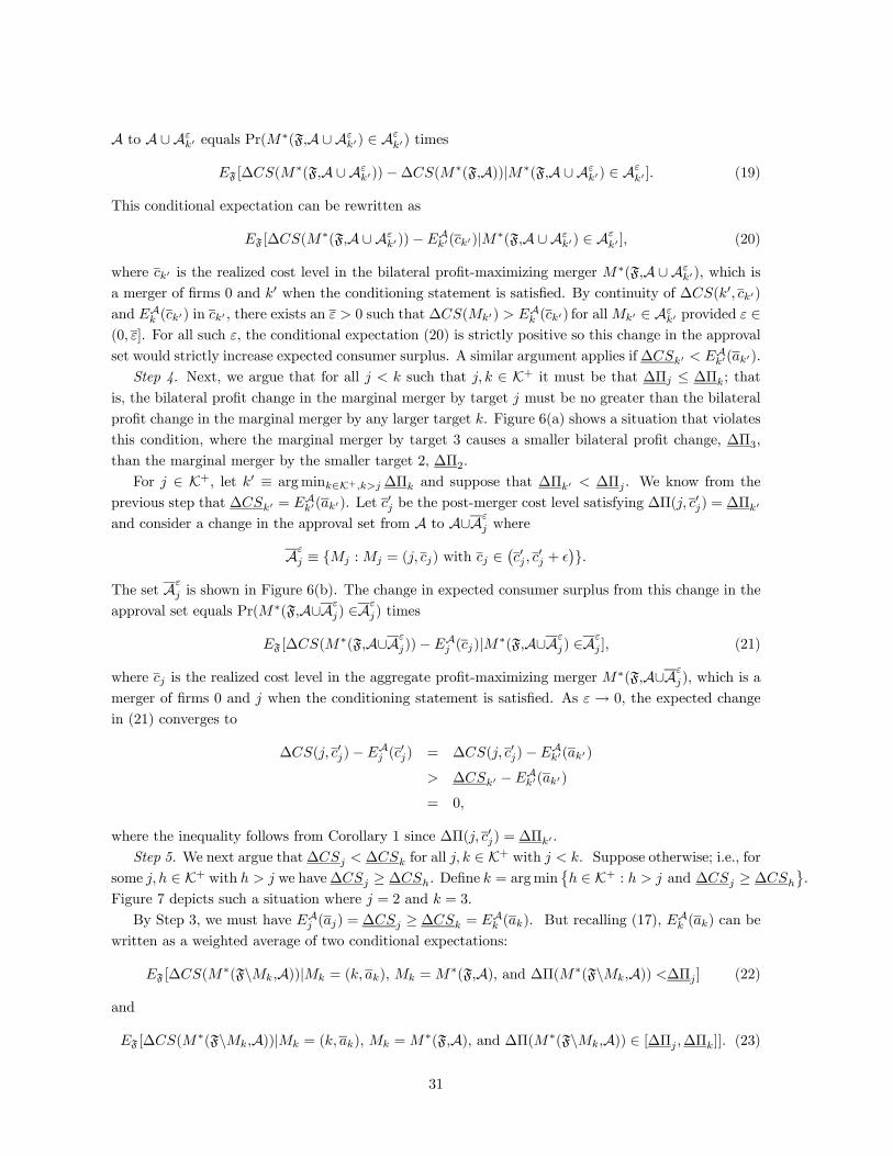
A to A ∪Aεk0 equals Pr(M

∗(F,A ∪Aεk0) ∈ A

εk0) times

EF [∆CS(M∗(F,A ∪Aε

k0))−∆CS(M∗(F,A))|M∗(F,A ∪Aεk0) ∈ A

εk0 ]. (19)

This conditional expectation can be rewritten as

EF [∆CS(M∗(F,A ∪Aε

k0))−EAk0(ck0)|M∗(F,A ∪Aεk0) ∈ A

εk0 ], (20)

where ck0 is the realized cost level in the bilateral profit-maximizing merger M∗(F,A ∪Aεk0), which is

a merger of firms 0 and k0 when the conditioning statement is satisfied. By continuity of ∆CS(k0, ck0)and EAk (ck0) in ck0 , there exists an ε > 0 such that ∆CS(Mk0) > EAk (ck0) for allMk0 ∈ Aε

k0 provided ε ∈(0, ε]. For all such ε, the conditional expectation (20) is strictly positive so this change in the approvalset would strictly increase expected consumer surplus. A similar argument applies if ∆CSk0 < EAk0(ak0).Step 4. Next, we argue that for all j < k such that j, k ∈ K+ it must be that ∆Πj ≤ ∆Πk; that

is, the bilateral profit change in the marginal merger by target j must be no greater than the bilateralprofit change in the marginal merger by any larger target k. Figure 6(a) shows a situation that violatesthis condition, where the marginal merger by target 3 causes a smaller bilateral profit change, ∆Π3,than the marginal merger by the smaller target 2, ∆Π2.For j ∈ K+, let k0 ≡ argmink∈K+,k>j ∆Πk and suppose that ∆Πk0 < ∆Πj . We know from the

previous step that ∆CSk0 = EAk0(ak0). Let c0j be the post-merger cost level satisfying ∆Π(j, c

0j) = ∆Πk0

and consider a change in the approval set from A to A∪Aεj where

Aε

j ≡ {Mj :Mj = (j, cj) with cj ∈¡c0j , c

0j +

¢}.

The set Aε

j is shown in Figure 6(b). The change in expected consumer surplus from this change in theapproval set equals Pr(M∗(F,A∪Aε

j) ∈Aεj) times

EF [∆CS(M∗(F,A∪Aε

j))−EAj (cj)|M∗(F,A∪Aεj) ∈A

εj ], (21)

where cj is the realized cost level in the aggregate profit-maximizing merger M∗(F,A∪Aε

j), which is amerger of firms 0 and j when the conditioning statement is satisfied. As ε → 0, the expected changein (21) converges to

∆CS(j, c0j)−EAj (c0j) = ∆CS(j, c0j)−EAk0(ak0)

> ∆CSk0 −EAk0(ak0)

= 0,

where the inequality follows from Corollary 1 since ∆Π(j, c0j) = ∆Πk0 .Step 5. We next argue that∆CSj < ∆CSk for all j, k ∈ K+ with j < k. Suppose otherwise; i.e., for

some j, h ∈ K+ with h > j we have∆CSj ≥ ∆CSh. Define k = argmin©h ∈ K+ : h > j and ∆CSj ≥ ∆CSh

ª.

Figure 7 depicts such a situation where j = 2 and k = 3.By Step 3, we must have EAj (aj) = ∆CSj ≥ ∆CSk = EA

k (ak). But recalling (17), EAk (ak) can be

written as a weighted average of two conditional expectations:

EF [∆CS(M∗(F\Mk,A))|Mk = (k, ak), Mk =M∗(F,A), and ∆Π(M∗(F\Mk,A)) <∆Πj ] (22)

and

EF [∆CS(M∗(F\Mk,A))|Mk = (k, ak), Mk =M∗(F,A), and ∆Π(M∗(F\Mk,A)) ∈ [∆Πj ,∆Πk]]. (23)

31

Expectation (22) conditions on the event that the next-most-profitable merger other than (k, ak) inducesa bilateral profit change less than ∆Πj , the bilateral profit change of merger (j, aj). Since no merger inA by either target k or j can have such a profit level (since ∆Πk ≥ ∆Πj by Step 4), the expectation (22)must exactly equal EAj (aj). Now consider the expectation (23). If ∆Π(M

∗(F\Mk,A)) ∈ [∆Πj ,∆Πk),it could be that (i) M∗(F\Mk,A) = (j, cj) for some cj ≤ aj , or (ii) M∗(F\Mk,A) = (r, cr) for somer < j, or (iii) M∗(F\Mk,A) = (r, cr) for some r > j and r < k. Now, in case (i) it is immediatethat ∆CS(M∗(F\Mk,A) ≥ CSj , with strict inequality whenever cj = aj . In case (ii), the fact that∆Π(r, cr) ≥ ∆Πj implies by Corollary 1 that

∆CS(M∗(F\Mk,A) = ∆CS(r, cr) > CSj = EAj (aj). (24)

In case (iii), (24) follows from the definition of k. Thus, expectation (23) must strictly exceed EAj (aj),which leads to a contradiction.Step 6. Finally, we argue that K+ = {1, ..., bK} for some bK ≤ K. To establish this fact, we show

that if k /∈ K+ and k < K, then k + 1 /∈ K+. We first observe that ∆CS(k, l) > ∆CS(k + 1, l),which follows because the profile of firms’ costs following merger (k, l) are lower than following merger(k + 1, l) (the post-merger industry cost profile differs only for firms k and k + 1, which have costsof l and ck+1 with the first merger and ck and l with the second). Thus, if k + 1 ∈ K+, then∆CS(k + 1, ak+1) < ∆CS(k, l). But, an argument like that in Step 5 [using the fact that, by anargument like that in Step 3, ∆CS(k, l) ≤ EAk (ak)] shows that ∆CS(k, l) < EAk+1(ak+1), so that∆CS(k + 1, ak+1) < EAk+1(ak+1), contradicting the conclusion of Step 3.

Proof of Proposition 2. Denote byA∗(∆Π|J) a policy that is an element of argmaxA⊆Πk∈J [l,hk]ECS(∆Π;A, J)for a given J and ∆Π. Also, define P (∆Π|J,A) ≡ {k ∈ J : ∆Π(k, ak) < ∆Π} as the set of targets inJ who may have an acceptable merger with profit below ∆Π under policy A ⊆ Πk∈J [l, hk]. Note thatchanges to A that alter acceptance sets only for k /∈ P (∆Π|J,A) and leave P (∆Π|J,A) unchangedhave no effect on the value of ECS(∆Π;A, J). Finally, for any set A, let AJ ≡ Πj∈JAj .With these preliminaries, we now establish the result. Observe first that, for any J , a sufficient condi-

tion forMk with k ∈ J and∆Π(Mk) < ∆Π to be approved in any solution tomaxA⊆Πj∈J [l,hj ]ECS(∆Π;A, J)is that its CS-level, ∆CS(Mk), strictly exceeds maxA⊆Πj∈J\k[l,hj ]ECS(∆Π(Mk);A, J\k). We will es-tablish the result through an induction argument that shows that for all ∆Π and any J such that 1 ∈ J ,if A∗(∆Π|J) ∈ argmaxA⊆Πj∈J [l,hj ]ECS(∆Π;A, J) then

P (∆Π|J,A∗(∆Π|J)) = P (∆Π|J,AC(J)) (25)

andA∗k(∆Π|J) = AC

k (J) for all k ∈ P (∆Π|J,AC(J)). (26)

That is, any policy A that maximizes ECS(∆Π;A, J) accepts with positive probability [conditional onthe most profitable acceptable merger having ∆Π(Mj) ≤ ∆Π] mergers involving the same set of targetsas does the cutoff policy AC(J), and coincides with the cutoff policy AC(J) for all such targets. Inparticular, this implies that the cutoff policy AC(J) ∈ argmaxA⊆Πk∈J [l,hk]ECS(∆Π,A, J) for all ∆Πand any J such that 1 ∈ J . Taking ∆Π =∞ and J = K will then yield the result.Consider first the set J = {1}. Then, we have aC1 (J) = bc1(Q0). Moreover, it is immediate — given

our earlier discussion — that (25) and (26) hold for all ∆Π.

32

Now consider any set J = Jn with #Jn = n and 1 ∈ Jn, and assume:Induction Hypothesis 1: Properties (25) and (26) hold for any set J = Jn0 with 1 ∈ Jn0 and

n0 < n.Number the targets in set Jn in increasing order of their pre-merger market share as (1, ..., n). If

P (∆Π|J,AC(J)) = ∅, then ∆Π ≤ ∆Π(1,bc1(Q0)). From Proposition 1, it follows immediately that

P (∆Π|J,A∗(∆Π|J)) = ∅. Hence, properties (25) and (26) hold for set Jn.So suppose now instead that P (∆Π|J,AC(J)) 6= ∅. Note that, since ∆Π(k, aCk (J)) is increasing in

k, the set P (∆Π|J,AC(J)) is of the form P (∆Π|J,AC(J)) = {1, ...,bj(∆Π)} for some bj(∆Π).Consider first the treatment of mergers with target 1. We have aC1 (J) = bc1(Q0). Moreover, the

following two properties hold for all ∆Π: for any A∗(∆Π|Jn) ∈ argmaxA⊆Πj∈Jn [l,hj ]ECS(∆Π;A, Jn),

1 ∈ P (∆Π|Jn,A∗(∆Π|Jn))⇔ 1 ∈ P (∆Π|Jn,AC(Jn)) (27)

andA∗1(∆Π|Jn) = AC

1 (Jn) if 1 ∈ P (∆Π|Jn,AC(Jn)). (28)

These follow from the following facts: (i) No CS-decreasing merger M1 can be accepted in A∗(∆Π|Jn);(ii) for any A ⊆ Πj∈Jn [l, hj ], ECS(∆Π(1, c1);A, Jn) < ∆CS(1, c1) for all c1 < bc1(Q0), so all mergersM1 = (1, c1) such that c1 < bc1(Q0) and ∆Π(1, c1) ≤ ∆Π must be in A∗(∆Π|Jn), and (iii) acceptingall mergers M1 such that ∆Π(1, c1) > ∆Π maximizes Pr(∆Π(M1) > ∆Π and M1 ∈ A1) and, sinceaccepting the mergers described in (ii) is optimal, therefore maximizes ECS(∆Π;A, Jn).Now, consider a merger with target k > 1 and assume:Induction Hypothesis 2: For all k0 < k, the following two properties hold for all ∆Π: for any

A∗(∆Π|Jn) ∈ argmaxA⊆Πj∈Jn [l,hj ]ECS(∆Π;A, Jn),

k0 ∈ P (∆Π|Jn,A∗(∆Π|Jn))⇔ k0 ∈ P (∆Π|Jn,AC(Jn)) (29)

andA∗k0(∆Π|Jn) = AC

k0(Jn) if k0 ∈ P (∆Π|Jn,AC(Jn)). (30)

We will show that properties (29) and (30) hold as well for k so that Induction Hypothesis 2holds for k + 1. Suppose, first, that k /∈ P (∆Π|Jn, AC(Jn)). Then every Mk with ∆Π(Mk) ≤ ∆Πhas ECS(∆Π(Mk);AC

Jn\k(Jn), Jn\k) > ∆CS(Mk). But by Induction Hypothesis 2 and Proposition1 [which implies that in A∗(∆Π|Jn) we must have ∆Πk < ∆Πj for any j > k such that j ∈P (∆Π|Jn,A∗(∆Π|Jn))], which implies thatECS(∆Π(Mk);A∗Jn\k(∆Π|Jn), Jn\k) = ECS(∆Π(Mk);AC

Jn\k(Jn), Jn\k).Hence, merger Mk cannot be in A∗(∆Π|Jn); i.e., k /∈ P (∆Π|Jn,A∗(∆Π|Jn)).Suppose now instead that k ∈ P (∆Π|J,AC(Jn)). Observe, first, that every Mk = (k, ck) with ck >

aCk (Jn) has ECS(∆Π(Mk);ACJn\k(Jn), Jn\k) > ∆CS(Mk), and since by Induction Hypothesis 2 and

Proposition 1, ECS(∆Π(Mk);A∗Jn\k(∆Π|Jn), Jn\k) = ECS(∆Π(Mk);ACJn\k(Jn), Jn\k), the merger

cannot be in A∗(∆Π|Jn); i.e., A∗k(∆Π|Jn) ⊆ ACk (Jn). Next, consider mergers Mk = (k, ck) with ck <

aCk (Jn). Condition (9) combined with Induction Hypotheses 1 and 2 imply that each of these mergerssatisfies ∆CS(Mk) > ECS(∆Π(Mk);AC(Jn\k), Jn\k) = maxA⊆Πj∈Jn\k[l,hj ]ECS(∆Π(Mk),A, Jn\k),and hence must be included in A∗(∆Π|Jn); i.e., AC

k (Jn) ⊆ A∗k(∆Π|Jn). We thus have ACk (Jn) =

A∗k(∆Π|Jn). Hence, properties (29) and (30) hold as well for k. Applying induction (twice) then yieldsthe result.

33

Proof of Proposition 3. LetA denote the optimal approval policy with cutoffs (a1, ..., aK)when Pr(φk =1) = θk, and let A0 denote the optimal approval policy with cutoffs (a01, ..., a0K) when Pr(φk = 1) = θ0k.From the recursive definition of the cutoffs, it follows immediately that a change in θk does not affect thecutoffs for any smaller merger Mj , j < k , nor the cutoff of merger Mk itself. Hence, ∆CSj

0 = ∆CSjfor all j ≤ k.

Consider now the cutoff for merger Mk+1, k + 1 ≤ K̂. We can write the cutoff condition as

∆CSk+1 = Pr(φk = 1| ∆Π¡M∗

¡F{1,...,k},A{1,...,k}

¢¢≤ ∆Π(k + 1, ak+1))

×EF{1,...,k}£∆CS

¡M∗

¡F{1,...,k},A{1,...,k}

¢¢|

∆Π¡M∗

¡F{1,...,k},A{1,...,k}

¢¢≤ ∆Π(k + 1, aj+1) and φk = 1

¤+£1− Pr(φk = 1| ∆Π

¡M∗

¡F{1,...,k},A{1,...,k}

¢¢≤ ∆Π(k + 1, ak+1)

¤×EF{1,...,k}

£∆CS

¡M∗

¡F{1,...,k},A{1,...,k}

¢¢|

∆Π¡M∗

¡F{1,...,k},A{1,...,k}

¢¢≤ ∆Π(k + 1, ak+1) and φk = 0

¤,

where AJ ≡ Πj∈JAj .

Note first that the optimal policy must be such that

EF{1,...,k}£∆CS

¡M∗

¡F{1,...,k},A{1,...,k}

¢¢|Mk+1 = (k + 1, ak+1),

∆Π¡M∗

¡F{1,...,k},A{1,...,k}

¢¢≤ ∆Π(Mk+1), and φk = 1

¤> EF{1,...,k}

£∆CS

¡M∗

¡F{1,...,k},A{1,...,k}

¢¢|Mk+1 = (k + 1, ak+1),

∆Π¡M∗

¡F{1,...,k},A{1,...,k}

¢¢≤ ∆Π(Mk+1), and φk = 0

¤.

To see this, consider the case where φk = 1 and ∆Π¡M∗

¡F{1,...,k},A{1,...,k}

¢¢≤ ∆Π(k + 1, ak+1).

Two cases can arise: (i) M∗¡F{1,...,k},A{1,...,k}

¢6=Mk and (ii) M∗

¡F{1,...,k},A{1,...,k}

¢=Mk. In case

(i) the outcome is the same as when Mk were not feasible (φk = 0). In case (ii), merger Mk will beimplemented. If merger Mk were not feasible, we would instead obtain the expected consumer surplusof the next most profitable allowable merger. By the optimality of the approval policy, ∆CS(Mk) mustweakly exceed (and, generically, strictly) the expected consumer surplus of the next-most profitableallowable merger.Next, note that we can rewrite the conditional probability as

Pr(φk = 1|∆Π¡M∗

¡F{1,...,k},A{1,...,k}

¢¢≤ ∆Π(k + 1, ak+1))

= Pr( ∆Π¡M∗

¡F{1,...,k},A{1,...,k}

¢¢≤ ∆Π(k + 1, ak+1)|φk = 1)θk

שPr(∆Π

¡M∗

¡F{1,...,k},A{1,...,k}

¢¢≤ ∆Π(k + 1, ak+1)|φk = 1)θk

+Pr(∆Π¡M∗

¡F{1,...,k},A{1,...,k}

¢¢≤ ∆Π(k + 1, ak+1)|φk = 0)(1− θk)

ª−1=

(1 +

Pr(∆Π¡M∗

¡F{1,...,k},A{1,...,k}

¢¢≤ ∆Π(k + 1, ak+1)|φk = 0)

Pr(∆Π¡M∗

¡F{1,...,k},A{1,...,k}

¢¢≤ ∆Π(k + 1, ak+1)|φk = 1)

µ1− θkθk

¶)−1.

Hence, an increase in θk induces an increase in the conditional probability Pr(φk = 1|∆Π¡M∗

¡F{1,...,k},A{1,...,k}

¢¢≤

∆Π(k + 1, ak+1)). But this implies that an increase in θk induces an increase in the RHS of the cutoffcondition for merger Mk+1. Hence, ∆CS

0k+1 > ∆CSk+1.

Consider now the induction hypothesis that ∆CS0k0 > ∆CSk0 for all k < k0 < j ≤ K̂. In particular,∆CS0j−1 > ∆CSj−1. We claim that this implies that ∆CS0j > ∆CSj . To see this, note that we can

34

decompose the effect of the increase in θk on the conditional expectation of the next-most profitablemerger into two steps:

1. Increase the feasibility probability from θk to θ0k > θk, holding fixed the approval policy A.

2. Change the approval policy from A to A0.

Consider first step (1). For the same reason as before, the increase in the feasibility probabilitymust raise the conditional expectation

EF{1,...,j−1}£∆CS

¡M∗

¡F{1,...,j−1},A{1,...,j−1}

¢¢| ∆Π

¡M∗

¡F{1,...,j−1},A{1,...,j−1}

¢¢≤ ∆Π(j, aj)

¤by the optimality of the approval policy A.Consider now step (2). The outcome under the two policies differs only in the event where

M∗¡F{1,...,j−1},A{1,...,j−1}

¢/∈ A0. Let Mi = M∗

¡F{1,...,j−1},A{1,...,j−1}

¢. Under policy A, the out-

come in this event is ∆CS(Mi). Under policy A0 instead, the expected outcome is

EF{1,...,i−1}

h∆CS

³M∗

³F{1,...,i−1},A0{1,...,i−1}

´´| ∆Π

³M∗

³F{1,...,i−1},A0{1,...,i−1}

´´≤ ∆Π(k, ci)

i.

But as Mi /∈ A0, we must have

EF{1,...,i−1}

h∆CS

³M∗

³F{1,...,i−1},A0{1,...,i−1}

´´| ∆Π

³M∗

³F{1,...,i−1},A0{1,...,i−1}

´´≤ ∆Π(j, ci)

i> ∆CS(Mi).

As the expected consumer surplus increases at each step, we must have ∆CS0j > ∆CSj .

Proof of Proposition 4. A change in firm 0’s marginal cost does not affect the outcome (consumer

surplus, profits) after any merger Mk, k ≥ 1, but it does affect the pre-merger outcome. In particular,we have Q00 > Q0 so that γ ≡ CS00 − CS0 > 0. Let ηk ≡ [π000 + π00k ] − [π00 + π0k] denote the inducedchange in the joint pre-merger profit of firms 0 and k. The key observation is that the profit of a moreefficient firm falls by a larger amount than that of a less efficient as price falls. That is, ηk is decreasingin k.Consider first merger M1. We have ∆CS(1, a01)

0 = ∆CS(1, a01) − γ = 0. Hence, ∆CS(1, a01) >∆CS(1, a1) = 0, implying that a01 < a1. Consider now the (marginal) merger M2 = (2, a2). Let (1,ea1)be such that ∆Π(1,ea1) = ∆Π(2, a2), and (1,ea01) be such that ∆Π(1,ea01)0 = ∆Π(2, a2)0. We have

∆Π(1,ea1)0 = ∆Π(1,ea1)− η1

< ∆Π(1,ea1)− η2

= ∆Π(2, a2)− η2

= ∆Π(2, a2)0

= ∆Π(1,ea01)0,where the inequality follows from η1 > η2. Hence, ea01 < ea1. That is, before the reduction in c0, anymerger M1 with c1 ≥ ea1 induced a smaller increase in bilateral profit than merger M2 = (2, a2). Afterthe reduction in c0, this is still true, but now — in addition — any merger M1 with ea1 > c1 ≥ ea01 alsoinduces a smaller increase in bilateral profit than merger M2 = (2, a2). That is, there are now more

35

and (in an FOSD sense) more efficient mergers M1 that are less profitable than M2 = (2, a2). Sincethe induced CS-increase of merger M1 is the greater, the lower is c1, we thus have again that

EF{1}

∙∆CS

³M∗

³F{1},A0{1}

´´0| ∆Π

µM∗

³F{1},A0{1}

´0¶≤ ∆Π(2, a2)0

¸> EF{1}

£∆CS

¡M∗

¡F{1},A{1}

¢¢| ∆Π

¡M∗

¡F{1},A{1}

¢¢≤ ∆Π(2, a2)

¤− γ

= ∆CS(2, a2)− γ

= ∆CS(2, a2)0.

Hence, a02 < a2. Under the induction hypothesis that a0j < aj for every j < k ≤ K̂ , a similar argumentcan be used to show that a0k < ak.

Lemma 7. Consider the function H(s1, ..., sN ) =P

n(sn)2 and two vectors s0 = (s01, ..., s

0N ) and

s00 = (s001 , ..., s00N ) having

PNn=1 s

0n =

PNn=1 s

00n. If for some r, (i) s

0r ≥ s0j for all j 6= r, (ii) s00r > s0r, and

(iii) s00j ≤ s0j for all j 6= r, then H(s00) > H(s0).

Proof. Without loss of generality, take r = 1 and define ∆n ≡ s0n − s00n for n > 1. Observe that ∆n ≥ 0for all n > 1 and ∆n > 0 for some n > 1. Define as well the vectors sn ≡ (s01+

Pnt=2∆t, s

02−∆2, ..., s0n−

∆n, s0n+1, ..., s

0N ) for n > 1 and s1 ≡ s0. Note that sN = s00. Then

H(s00)−H(s0) =N−1Xn=1

[H(sn+1)−H(sn)].

Now letting s11 ≡ s01 and sn1 ≡ s01 +Pn

t=2∆t ≥ s01 for all n > 1, each term in this sum is nonnegative,

H(sn+1)−H(sn) = (sn1 +∆n+1)2 + (s0n+1 −∆n+1)

2 − (sn1 )2 − (s0n+1)2

= 2∆n+1(sn1 − s0n+1) + 2(∆n+1)

2 ≥ 0,

and strictly positive if ∆n+1 > 0. Since ∆n+1 > 0 for some n ≥ 1, the result follows.

Proof of Lemma 4. From the discussion in the main text, the post-merger aggregate profit is given by(10). As both mergers induce the same level of consumer surplus (and thus the same Q), the first termon the right-hand side of (10) is the same for both mergers. It thus suffices to show that the largermerger Mk induces a larger value of H than the smaller merger Mj .Now, as both mergers induce the same Q, Assumption 1 implies that the output of any firm not

involved in Mj or Mk is the same under both mergers. Hence,

sk(Mk) + sj(Mk) = sk(Mj) + sj(Mj). (31)

Next, recall that a CS-nondecreasing merger increases the share of the merging firms and reduces theshare of all nonmerging firms. Thus, we have sk(Mk) ≥ sk + s0 > sk(Mj) and sj(Mj) ≥ sj + s0 >

sj(Mk). In addition, since total output is the same after both mergers and ck < cj , we also havesj(Mk) < sk(Mj). By (31), this in turn implies that sk(Mk) > sj(Mj). Hence, the distribution of

market shares after the larger merger Mk is a sum-preserving spread of those after the smaller mergerMj :

sk(Mk) > max{sj(Mj), sk(Mj)} ≥ min{sj(Mj), sk(Mj)} > sj(Mk). (32)

By Lemma 7 in the Appendix (just above), H is therefore larger after Mk than after Mj .

36

Lemma 8. The slope of the curve for merger Mk in (∆Π,∆CS)-space is given by

d∆Π(Mk)

d∆CS(Mk)= −2−

∙P 00(Q(Mk))Q(Mk)

P 0(Q(Mk))

¸H(Mk) +

∙2

P 0(Q(Mk))Q(Mk)

¸ ∙r(Q(Mk); cMk

)

dQ(Mk)/dcMk

¸,

where r(Q; c) ≡ {q|P (Q)− c+ qP 0(Q) = 0} is the “cumulative best reply” of a firm with marginal costc to aggregate output Q.

Proof. The change in ∆CS induced by a small increase in post-merger marginal cost is

d∆CS(Mk)

dcMk

= −P 0(Q)Q dQ

dcMk

,

where Q ≡ Q(Mk) is aggregate output following mergerMk. Recall that aggregate profit can be writtenas η(Q)H, where H ≡ H(Mk) is the post-merger Herfindahl index and η(Q) ≡ −P 0(Q)Q2. The effectof a small increase in post-merger marginal cost on the change in aggregate profit induced by mergerMk is thus given by

d∆Π(Mk)

dcMk= η0(Q)

dQ

dcMk

H + η(Q)dH

dcMk

,

whereη0(Q) = −[P 00(Q)Q2 + 2P 0(Q)Q].

Putting this together, we obtain

d∆Π(Mk)

d∆CS(Mk)= −

∙η0(Q)

P 0(Q)Q

¸H −

∙η(Q)

P 0(Q)Q

¸(dH/dcMk

)

(dQ/dcMk)

=

∙2 +

P 00(Q)Q

P 0(Q)

¸H +Q

(dH/dcMk)

(dQ/dcMk)(33)

Now, we have

dH

dcMk

=d

dcMk

"Pi r(Q; ci)

2

Q2

#

= −Ã2

Q3

!dQ

dcMk

"Xi

r(Q; ci)2

#+

Ã1

Q2

!(2r(Q; cMk

)∂r(Q; cMk)

∂cMk

+ 2Xi

r(Q; ci)dr(Q; ci)

dQ

dQ

dcMk

)

= −µ2

Q

¶H

dQ

dcMk

+

Ã2

P 0(Q)Q2

!r(Q; cMk)−

Ã2

Q2

!dQ

dcMk

Xi

∙r(Q; ci) +

P 00(Q)

P 0(Q)r(Q; ci)

2

¸

= −µ2

Q

¶H

dQ

dcMk

+

Ã2

P 0(Q)Q2

!r(Q; cMk

)−µ2

Q

¶dQ

dcMk

− 2P00(Q)

P 0(Q)H

dQ

dcMk

, (34)

where the third equality follows using the facts that ∂r(Q; cMk)/∂cMk

= 1/P 0(Q) and dr(Q; ci)/dQ =

−¡1 + r(Q; ci)P

00(Q)/P 0(Q)¢. Thus, we have:

Q(dH/dcMk

)

(dQ/dcMk)= −2H − 2− 2

µP 00(Q)Q

P 0(Q)

¶H +

µ2

P 0(Q)Q

¶r(Q; cMk

)¡dQ/dcMk

¢ . (35)

Substituting (35) into (33), we obtain equation (11).

37

Proof of Lemma 5. Let Q ≡ Q(Mk) denote post-merger aggregate output. Inserting

dQ

dcMk

=1

(N −mk + 3)P 0(Q) +QP 00(Q)

into equation (11), we obtain

d∆Π(Mk)

d∆CS(Mk)= −2− QP 00(Q)

P 0(Q)H +

2sMk

P 0(Q)

£(N −mk + 3)P

0(Q) +QP 00(Q)¤

= 2 [(N −mk + 3)sMk− 1] + QP 00(Q)

P 0(Q)

£2sMk

−H¤,

where sMkis the actual market share of the merged firm and H ≡ H(Mk) the actual post-merger

Herfindahl index.Now, we claim that snaiveMk

≥ Hnaive(Mk)/2 implies that 2sMk≥ H. To see this, note that the

naively-computed inequality snaiveMk≥ Hnaive(Mk)/2 corresponds to the case of a CS-neutral merger.

As merger Mk is CS-nondecreasing by assumption, it involves a (weakly) lower level of cMk(and a

weakly greater level of aggregate output) than a CS-neutral merger. It therefore suffices to show thata small reduction in cMk leads to a larger value of

£2sMk −H

¤, i.e., d

£2sMk −H

¤> 0. But we have

d£2sMk −H

¤= 2dsMk − 2

⎛⎝sMkdsMk +Xi/∈Mk

sidsi

⎞⎠= 2(1− sMk

)

⎛⎝1− Xi/∈Mk

dsi

⎞⎠− 2 Xi/∈Mk

sidsi

> 0,

where the inequality follows from the observation that the induced increase in aggregate output reducesthe market share of each nonmerging firm i, i.e., dsi < 0.Since Assumption 1 implies that QP 00(Q)/P 0(Q) > −1, we obtain

d∆Π(Mk)

d∆CS(Mk)≥ 2 [(N −mk + 3)sMk

− 1]−£2sMk

−H¤

= 2 [(N −mk + 2)sMk− 1] +H.

The r.h.s. of the last equation is positive if and only if

H

2≥ 1− (N −mk + 2)sMk .

We claim that this inequality is implied by the naively-computed analog,

Hnaive(Mk)

2≥ 1− (N −mk + 2)s

naiveMk

.

38

To see this, consider the effect of decreasing the post-merger marginal cost cMkon£H − 2 (1− (N −mk + 2)sMk

)¤:

d£H − 2 (1− (N −mk + 2)sMk

)¤= 2

⎛⎝sMkdsMk

+Xi/∈Mk

sidsi

⎞⎠+ 2(N −mk + 2)dsMk

= 2(N −mk + 2 + sMk)

⎛⎝1− Xi/∈Mk

dsi

⎞⎠+ 2 Xi/∈Mk

sidsi

= 2

⎧⎨⎩(N −mk + 2 + sMk)−

Xi/∈Mk

(N −mk + 2 + sMk− si)dsi

⎫⎬⎭> 0,

where the inequality follows from the observation that dsi < 0 for all i /∈Mk and N −mk +2 ≥ 1.

Proof of Lemma 6. Let q0Ml≡P

i∈Mlq0i , l = j, k. The pre-merger first-order conditions imply that

[mlP (Q0)−

Xi∈Ml

ci] + P 0(Q0)q0Ml= 0 for l = j, k,

so(mk −mj)P (Q

0)−Xi∈Mk

ci +Xi∈Mj

ci = P 0(Q0)(q0Mj− q0Mk

) > 0. (36)

Next, summing up the post-merger first-order conditions, we have

(N −ml + 2)P (Q)−Xi

ci +Xi∈Ml

ci − cMl+ P 0(Q)Q = 0 for l = j, k, (37)

where N + 1 is the number of firms prior to any merger. So,

−

⎡⎣(mk −mj)P (Q)−Xi∈Mk

ci +Xi∈Mj

ci

⎤⎦− [cMk− cMj

] = 0.

Since −(mk −mj)P (Q) ≤ −(mk −mj)P (Q) as the mergers are CS-nondecreasing by assumption, wehave

−

⎡⎣(mk −mj)P (Q)−Xi∈Mk

ci +Xi∈Mj

ci

⎤⎦− [cMk − cMj ] ≥ 0,

so (36) implies that cMk− cMj < 0, which in turn implies that r(Q; cMk

) > r(Q; cMj ).Applying the implicit function theorem to (37), yields

dQ

dcMl

=1

(N −ml + 3)P 0(Q) +QP 00(Q).

As mk ≤ mj , P 0(Q) < 0, P 0(Q) +QP 00(Q) < 0, and (from above) r(Q; cMk) > r(Q; cMj

), we obtain

−r(Q; cMk)

dQ/dcMk

> −r(Q; cMj )

dQ/dcMj

.

Equation (11) implies that d∆Π/d∆CS is larger for merger Mk than for Mj at any point where thecurves cross, from which the assertion follows.

39

Proof of Lemma 4’. The proof proceeds exactly as that of Lemma 4, except that the inequalitiessk(Mk) > sk(Mj) and sj(Mj) > sj(Mk) in equation (32) now hold because, by Assumption 3’, anyW-nondecreasing merger involves synergies (ck < ck and cj < cj).

Proof of Proposition 5. Steps 1-2 proceed along the same lines as those in the proof of Proposition 1.Step 3. As in the absence of fixed cost savings, any optimal policy has the property that, for all

k ∈ K+ and any fk, ∆CSk(fk) is equal to the expected change in consumer surplus from the next-mostprofitable merger M∗(F\(k, ak(fk), fk),A), conditional on the marginal merger Mk = (k, ak(fk), fk)

maximizing the change in the merging firms’ bilateral profit in F∩A. That is,

∆CSk(fk) = EAk (ak(fk), fk)

≡ EF [∆CS(M∗(F\Mk,A))|Mk = (k, ak(fk), fk) and ∆Π(M

∗(F\Mk,A)) ≤ ∆Π(Mk)].

To see that this equation must hold for all k ∈ K+, suppose first that ∆CSk0(f0k0) > EAk0(ak0(f

0k0), f

0k0)

for some firm k0 ∈ K+ and fixed cost realization f 0k0 , and consider the alternative approval set A ∪Aεk0 ,

where

Aεk0 ≡

nMk :Mk = (k

0, ck0 , fk0) with ck0 ∈³ak0(f

0k0), ak0(f

0k0) + ε

´and fk0 ∈

³f0k0 − ε, f

0k0 + ε

´o.

Using the same type of argument as in the proof of Proposition 1, it is straightforward to show that,

for ε > 0 small enough, the change in expected consumer surplus from changing the approval setfrom A to A ∪Aε

k0 is strictly positive. A similar logic can be used to show that we cannot have∆CSk0(f

0k0) < EAk0(ak0(f

0k0), f

0k0).

Step 4. LetMCSj ≡ {Mj : ∆CS(Mj) = ∆CSj and Mj ∈ Aj} denote the set of marginal mergers

Mj that induce a change in consumer surplus of∆CSj , and letMCSj ∈MCS

j denote the most profitableamong these mergers, i.e., ∆Π(MCS

j ) ≥ ∆Π(M 0j) for all M

0j ∈MCS

j . This merger is depicted in Figure12 for j = 2. An optimal approval set must have the property that, for all j < k such that j, k ∈ K+,we have ∆Π

¡MCS

j

¢≤ ∆Πk. The argument is similar to (but slightly more involved than) Step 4 in the

proof of Proposition 1: For j ∈ K+, let k0 ≡ argmink∈K+,k>j ∆Πk and suppose that, contrary to our

claim, ∆Πk0 < ∆Π(MCSj ). In Figure 12 we suppose that k0 = 3. Let MΠ

k0 = (k0, ak0(f

Π

k0), fΠ

k0) denotethe marginal merger Mk0 that induces the bilateral profit change ∆Πk0 , i.e., ∆Π

¡MΠ

k0¢= ∆Πk0 . By

Step 3, MΠk0 is uniquely defined, and ∆CSk0(M

Πk0) = EAk0

³ak0(f

Π

k0), fΠ

k0

´. Note that EAk0

³ak0(f

Π

k0), fΠ

k0

´can be written as a weighted average of

τ1 ≡ EF [∆CS(Mj ,A))|Mk0 =MΠk0 , Mj ∈M∗(F\Mk0 ,A), and ∆Π(M∗(F\Mk0 ,A)) ≤ ∆Π(Mk0)]

and

τ2 ≡ EF [∆CS(M∗(F\Mk0 ,A))|Mk0 =MΠ

k0 , Mj /∈M∗(F\Mk0 ,A), and ∆Π(M∗(F\Mk0 ,A)) ≤ ∆Π(Mk0)],

where the probability weight on τ1 is positive if and only if ∆Πj < ∆Πk0 . Note also that τ1 ≥ ∆CSj >∆CS

¡MΠ

k0¢= EAk0

³ak0(f

Π

k0), fΠ

k0

´. Hence, by Step 3,

∆CS¡MΠ

k0¢= EAk0

³ak0(f

Π

k0), fΠ

k0

´≥ τ2. (38)

40

ΠΔ

CSΔ 1M2M

MM

2CSΔ

3ΠΔ

)( 2CSMΠΔ

Π3M

CSM2

ε2A

Figure 12: The figure illustrates the change considered in Step 4 of the proof of Proposition 5

Consider a change in the approval set from A to A∪Aε

j , where

Aε

j ≡ {Mj : ∆Π(Mj) ∈ [∆Πk0 − ε,∆Πk0 ]},

and ε > 0. Note that, as shown in Figure 12, Aε

j * A. The change in expected consumer surplus fromthis change in the approval set equals Pr(M∗(F,A∪Aε

j) ∈(A∪Aε

j)\A) [which is strictly positive as Aε

j *A] times

EF [∆CS(M∗(F,A∪Aε

j))−EAj (cj , f j)|M∗(F,A∪Aε

j) ∈(A∪Aε

j)\A], (39)

where (cj , f j) is the pair of realized cost levels in the most profitable merger M∗(F,A∪Aε

j), which isa merger of firms 0 and j when the conditioning statement is satisfied. Now there exists a δ > 0 such

that for all ε > 0 the quantity in (39) is at least as large as

EF [∆CS(MΠk0) + δ −EAj (cj , f j)|M∗(F,A∪A

ε

j) ∈(A∪Aε

j)\A]. (40)

As ε→ 0, the quantity in (40) converges to [∆CS(MΠk0)− τ2] + δ > 0, so for small enough ε > 0 (38)

implies that this change in the acceptance set is strictly beneficial.Step 5. For all j, k ∈ K+, j < k, we must have ∆CSj < ∆CSk. Suppose otherwise so that for some

j, h ∈ K+, h > j, we have ∆CSj ≥ ∆CSh. Let k ≡ argmin{h ∈ K+ : h > j and ∆CSj ≥ ∆CSh}.Figure 13 shows such a case where j = 2 and k = 3. Let merger MCS

k ’s marginal and fixed costs becCSk = ak(f

CS

k ) and fCS

k , respectively. Given Step 4, EAk (ak(fCS

k ), fCS

k ) can be written as a weightedaverage of two conditional expectations:

EF [∆CS(M∗(F\Mk,A))|Mk = (k, c

CSk , f

CS

k ), Mk =M∗(F,A), and ∆Π(M∗(F\Mk,A))<∆Πj ] (41)

41

ΠΔ

CSΔ 1M2M

MM

3CSΔ

3ΠΔ

)( 2CSMΠΔ

Π3M

CSM22CSΔ

CSM3

Π2M

2ΠΔ

Figure 13: The figure shows the change considered in Step 5 of the proof of Proposition 5

and

EF

h∆CS(M∗(F\Mk,A))|Mk = (k, c

CSk , f

CS

k ), Mk =M∗(F,A),

and ∆Π(M∗(F\Mk,A)) ∈ [∆Πj ,∆Π(Mk)]¤. (42)

Now the term in (41) equals EAk (ak(fΠ

k ), fΠ

k ), which by Step 3 equals ∆CS(MΠj ), which in turn is at

least ∆CSj by definition. On the other hand, the term in (42) strictly exceeds ∆CSj . Together, this

implies that EAk (ak(fCS

k ), fCS

k ) > ∆CSj . Since, by Step 3, we must have ∆CSk = EAk (ak(fCS

k ), fCS

k ),this contradicts ∆CSj ≥ ∆CSk.Step 6. The argument proceeds proceeds along the same lines as that in the proof of Proposition

1.

7.2 Notes on the Aggregative Game Approach

Assumptions. Suppose an unmerged firm i’s profit can be written as

π(ψi, ci;Ψ),

where ψi ≥ 0 is firm i’s strategic variable, ci the firm’s constant marginal cost, and Ψ ≡P

j ψjan aggregator summarizing the “aggregate outcome.” The firm’s cumulative best reply, r(Ψ; ci) ≡argmaxψi π(ψi, ci;ψi +

Pj 6=i ψj), is assumed to be single-valued and decreasing in marginal cost ci.

Similarly, a merged firm k’s profit is given by 2π(ψk, ck;Ψ), and its cumulative best reply, r(Ψ; ck) ≡

42

argmaxψk 2π(ψk, ck; 2ψk+P

j 6=0,k ψj), is single-valued and decreasing in ck. Consumer surplus, denotedV (Ψ), is an increasing function of the aggregator and does not depend on the composition of theaggregator.Suppose that there exists a unique stable equilibrium. Let ψi(Mk) denote firm i’s equilibrium action

under market structureMk, and Ψ(Mk) ≡P

j ψj(Mk). Further, suppose that firm i’s equilibrium profit

can be written as

g(ψi(Mk);Ψ(Mk)) ≡ maxψi

π(ψi, ci;Ψ(Mk)) if firm i is unmerged;

g(2ψi(Mk);Ψ(Mk)) ≡ maxψi

2π(ψi, ci;Ψ(Mk)) if firm i = k is merged.

The equilibrium profit function g has the following properties: (i) g(0;Ψ) = 0; (ii) for 0 ≤ ψi ≤ Ψ,g(ψi;Ψ) is strictly increasing and strictly convex in ψi. We assume that a reduction in post-mergermarginal cost ck leads to (a) an increase in ψk(Mk) and in the aggregate outcome Ψ(Mk); (b) anincrease in ψk(Mk)/Ψ(Mk) and a decrease in ψj(Mk)/Ψ(Mk), j 6= 0, k; and (c) an increase in themerged firm’s equilibrium profit g(2ψk(Mk),Ψ(Mk)) and a reduction in any other firm i’s equilibriumprofit g(ψi(Mk);Ψ(Mk)).Our assumptions hold for several textbook models of competition.

Example 3 (Cournot). In the homogeneous goods Cournot model with constant marginal costs, letψi denote the output of plant i. All unmerged firms can be thought of as single-plant firms, whereas amerged firm can be thought of as running two plants at the same marginal cost (producing the same

output at both plants). We impose the same assumptions on demand as in the main text. The profitmaximization problem of a single-plant firm i with marginal cost ci can be written as

maxψi

⎡⎣P (ψi +Xj 6=i

ψj)− ci

⎤⎦ψi.From the first-order condition of profit maximization, P (Ψ) − ci + ψiP

0(Ψ) = 0, we can write theequilibrium profit under merger Mk as

g(ψi(Mk);Ψ(Mk)) = − [ψi(Mk)]2 P 0(Ψ(Mk)).

The profit maximization problem of a merged firm k with marginal cost ck (and two plants) can bewritten as

maxψk

⎡⎣P (2ψk + Xj 6=0,k

ψj)− ck

⎤⎦ 2ψk.From the first-order condition of profit maximization, P (Ψ)− ck+2ψkP

0(Ψ) = 0, so that we can writethe merged firm’s equilibrium profit under merger Mk as

g(2ψk(Mk);Ψ(Mk)) = − [2ψk(Mk)]2P 0(Ψ(Mk)).

It can easily be verified that g has all of the required properties (it takes the value of zero if its firstargument is zero and is increasing and convex in its first argument) and that a reduction in post-mergermarginal cost ck has the posited effects. (The other assumptions were shown to hold in the main text.)

43

Example 4 (CES). In the CES demand model with price competition, suppose that an unmergedfirm produces a single good, while a merged firm produces two goods at the same marginal cost(thus optimally charging the same price for each). Consider first a single-product firm i. The profitmaximization problem of a single-product firm i with marginal cost ci can be written as

maxψi[ψ−1/λi − ci]

ψ(λ+1)/λi

ψi +P

j 6=i ψj.

From the first-order condition of profit maximization,

−Ψ+hψ−1/λi − ci

iψ(λ+1)/λi

½(λ+ 1)Ψ

ψi− λ

¾= 0,

it can be seen that there is a unique cumulative best reply r(Ψ; ci) and that it is decreasing in thefirm’s marginal cost ci. We can write the firm’s equilibrium profit under merger Mk as

g (ψi(Mk);Ψ(Mk)) ≡½(λ+ 1)Ψ(Mk)

ψi(Mk)− λ

¾−1.

Consider now the merged firm k and suppose the firm produces two products at marginal cost ck. Theprofit maximization problem can be written as

maxψk

2[ψ−1/λk − ck]

ψ(λ+1)/λk

2ψk +P

j 6=0,k ψj.

(It can easily be verified that the firm optimally chooses the same value of ψk for each one of its twoproducts.) From the first-order condition,

−Ψ+hψ−1/λk − ck

iψ(λ+1)/λk

½(λ+ 1)Ψ

ψk− 2λ

¾= 0,

it can be seen that there is a unique cumulative best reply r(Ψ; ck) and that it is decreasing in ck. Wecan write the merged firm’s equilibrium profit under merger Mk as

g (2ψk(Mk);Ψ(Mk)) ≡½(λ+ 1)Ψ(Mk)

2ψk(Mk)− λ

¾−1.

It can easily be verified that our assumptions hold in the CES model. In particular, there exists aunique equilibrium and this equilibrium is stable.21 Moreover, the equilibrium profit function g has all

21From the first-order condition for profit maximization, we obtain that dr(Ψ; ci)/dΨ can be written as a decreasingand convex function of βi ≡ Ψ/r(Ψ; ci):

dr(Ψ; ci)

dΨ=

λ

(λ+ 1)βi(βi − 1) + λ.

This derivative attains its maximum of 1 if firm i is the only active firm (i.e., r(Ψ; ci) = Ψ). [Similarly, for a merged firmMk, we have

d2r(Ψ; ck)

dΨ=

λ

(λ+ 1)βk(βk − 1) + λ,

where βk ≡ Ψ/ [2r(Ψ; ck)].] It follows that i dr(Ψ; ci)/dΨ < 1 [resp. i 6=0,k dr(Ψ; ci)/dΨ + 2r(Ψ; ck)/dΨ < 1 aftermerger Mk] in any equilibrium with more than one active firm. Hence, any equilibrium must be stable. Moreover, asr(0; ci) ≥ 0 [resp. r(0; ck) ≥ 0] and r(Ψ; ci) = 0 [resp. r(Ψ; ck) = 0] for Ψ sufficiently large, this implies that there exists aunique Ψ that is consistent with equilibrium in the sense that Ψ− i r(Ψ; ci) = 0 [resp. Ψ− i6=0,k r(Ψ; ci)−2r(Ψ; ck) = 0after merger Mk].

44

of the required properties (it takes the value of zero if its first argument is zero and is increasing andconvex in its first argument). Consider a reduction in post-merger marginal cost ck. Since r(Ψ; ck) isdecreasing in ck and since r(Ψ; ci) and r(Ψ; ck) are increasing in Ψ, and since equilibrium is stable,the reduction in ck induces a higher value of Ψ = 2r(Ψ; ck) +

Pi6=0,k r(Ψ; ci). Rewrite the first-order

condition of an unmerged firm i:

−1 +h1− ci [r(Ψ; ci)]

1/λi½(λ+ 1)− λ

r(Ψ; ci)

Ψ

¾= 0.

As the induced increase in Ψ induces an increase in r(Ψ; ci) (i.e., prices are strategic complements), theratio r(Ψ; ci)/Ψ must fall as otherwise the l.h.s. of the first-order condition would decrease. But as

2r(Ψ; ck)

Ψ+

Pi6=0,k r(Ψ; ci)

Ψ= 1,

it follows that the same ratio for the merged firm, r(Ψ; ck)/Ψ, must increase. From the expression forthe equilibrium profits, we thus obtain that the profit of the merged firm, g (2r(Ψ(Mk); ck);Ψ(Mk)),increases and that of any unmerged firm i, g (r(Ψ(Mk); ci);Ψ(Mk)), decreases.

Example 5 (Multinomial Logit). In the multinomial logit demand model with price competition,suppose that an unmerged firm produces a single good, while a merged firm produces two goods at thesame marginal cost (and optimally charging the same price for each). Consider first a single-productfirm i. The profit maximization problem of a single-product firm i with marginal cost ci can be writtenas

maxψi

[a− μ lnψi − ci]ψi

ψi +P

j 6=i ψj

From the first-order condition of profit maximization,

{−μ+ a− μ lnψi − ci}Ψ− [a− μ lnψi − ci]ψi = 0,

it can be seen that there is a unique cumulative best reply r(Ψ; ci) and that it is decreasing in thefirm’s marginal cost ci. Firm i’s equilibrium profit under merger Mk can be written as

g(ψi(Mk);Ψ(Mk)) = μ

½Ψ(Mk)

ψi(Mk)− 1¾−1

.

Consider now the merged firm k and suppose the firm produces two products at marginal cost ck. Theprofit maximization problem can be written as

maxψk

2 [a− μ lnψk − ck]ψk

2ψk +P

j 6=0,k ψj.

(It can easily be verified that the firm optimally chooses the same value of ψk for each one of its twoproducts.) From the merged firm’s first-order condition of profit maximization,

{−μ+ a− μ lnψk − ck}Ψ− 2 [a− μ lnψk − ck]ψk = 0,

it can be seen that there is a unique cumulative best reply r(Ψ; ck) and that it is decreasing in ck. Firm

k’s equilibrium profit under merger Mk can be written as

g(2ψk(Mk);Ψ(Mk)) = μ

½Ψ(Mk)

2ψk− 1¾−1

.

45

It can easily be verified that our assumptions hold in the multinomial logit model. In particular, thereexists a unique equilibrium and this equilibrium is stable.22 Moreover, the equilibrium profit function ghas all of the required properties (it takes the value of zero if its first argument is zero and is increasingand convex in its first argument). Consider a reduction in post-merger marginal cost ck. Since r(Ψ; ck)is decreasing in ck and since r(Ψ; ci) and r(Ψ; ck) are increasing in Ψ, and since equilibrium is stable,

the reduction in ck induces a higher value of Ψ = 2r(Ψ; ck) +P

i6=0,k r(Ψ; ci). Rewrite the first-ordercondition of an unmerged firm i:

−1 +h1− ci [r(Ψ; ci)]

1/λi½(λ+ 1)− λ

r(Ψ; ci)

Ψ

¾= 0.

As the induced increase in Ψ induces an increase in r(Ψ; ci) (i.e., prices are strategic complements), theratio r(Ψ; ci)/Ψ must fall as otherwise the l.h.s. of the first-order condition would decrease. But as

−μ+ a− μ ln r(Ψ; ci)− cia− μ ln r(Ψ; ci)− ci

=r(Ψ; ci)

Ψ.

it follows that the same ratio for the merged firm, r(Ψ; ck)/Ψ, must increase. From the expression forthe equilibrium profits, we thus obtain that the profit of the merged firm, g (2r(Ψ(Mk); ck);Ψ(Mk)),increases and that of any unmerged firm i, g (r(Ψ(Mk); ci);Ψ(Mk)), decreases.

Results. Let ψ0i ≡ ψi(M0) and Ψ0 ≡ Ψ(M0), and note that, as consumer surplus V (Ψ) is strictlyincreasing in Ψ, merger Mk is CS-neutral if Ψ(Mk) = Ψ

0; it is CS-increasing if Ψ(Mk) > Ψ0, and

CS-decreasing if Ψ(Mk) < Ψ0.

Lemma 9. Merger Mk is CS-neutral if 2ψk(Mk) = ψ00 + ψ0k, CS-increasing if 2ψk(Mk) > ψ00 + ψ0k,and CS-decreasing if 2ψk(Mk) < ψ00 + ψ0k.

Proof. Suppose merger Mk is CS-neutral. Then, Ψ(Mk) = Ψ0. From the profit maximization problem

of any firm i not involved in the merger, it follows that ψi(Mk) = r (Ψ(Mk); ci) = r¡Ψ0; ci

¢= ψ0i .

Hence, we must have 2ψk(Mk) = ψ00+ψ0k. The claim then follows from the observation that consumersurplus is increasing in Ψ and that the equilibrium is stable.

Lemma 10. If merger Mk is CS-neutral, it raises the joint profit of the merging firms as well as

aggregate profit.

Proof. It is immediate to see that the profit of any firm not involved in the merger remains unchangedas Ψ remains unchanged. It thus remains to show that

g(2ψk(Mk);Ψ(Mk)) > g¡ψ00;Ψ

0¢+ g

¡ψ0k;Ψ

0¢.

22From the first-order condition for profit maximization, we obtain that dr(Ψ; ci)/dΨ can be written as a decreasingand convex function of βi ≡ Ψ/r(Ψ; ci):

dr(Ψ; ci)

dΨ=

1

βi(βi − 1) + 1.

This derivative attains its maximum of 1 if firm i is the only active firm (i.e., r(Ψ; ci) = Ψ). [Similarly, for a merged firmMk, we have

d2r(Ψ; ck)

dΨ=

1

βk(βk − 1) + 1,

where βk ≡ Ψ/ [2r(Ψ; ck)].] It follows that i dr(Ψ; ci)/dΨ < 1 [resp. i 6=0,k dr(Ψ; ci)/dΨ + 2r(Ψ; ck)/dΨ < 1 aftermerger Mk] in any equilibrium with more than one active firm. Hence, any equilibrium must be stable. Moreover, asr(0; ci) ≥ 0 [resp. r(0; ck) ≥ 0] and r(Ψ; ci) = 0 [resp. r(Ψ; ck) = 0] for Ψ sufficiently large, this implies that there exists aunique Ψ that is consistent with equilibrium in the sense that Ψ− i r(Ψ; ci) = 0 [resp. Ψ− i6=0,k r(Ψ; ci)−2r(Ψ; ck) = 0after merger Mk].

46

But as Mk is CS-neutral, we have Ψ(Mk) = Ψ0 and 2ψk(Mk) = ψ00 + ψ0k. The above inequality can

thus be rewritten asg¡ψ00 + ψ0k;Ψ

0¢> g

¡ψ00;Ψ

0¢+ g

¡ψ0k;Ψ

0¢.

But this follows from the assumed properties of the function g.

As a reduction in post-merger marginal cost increases the merged firm’s profit, any CS-nondecreasingmerger is profitable. As in the Cournot model with efficient bargaining (Section 5.1.1), we impose thefollowing assumption:

Assumption 4. If merger Mk, k ≥ 1, is CS-nondecreasing, then reducing its post-merger marginalcost ck increases the aggregate profit

hg(2ψk(Mk);Ψ(Mk)) +

Pi∈N\{0,k} g(ψi(Mk);Ψ(Mk))

i.

In the CES and multinomial logit models (and, as we have seen before, in the Cournot model), asufficient condition for this assumption to hold is that pre-merger cost differences are not too large sothat for every merger Mk,

¡ψ00 + ψ0k

¢/Ψ0 > maxi6=0,k ψ

0i /Ψ

0, i.e., the sum of the pre-merger shares ofthe merger partners exceeds the pre-merger share of the largest nonmerging firm.

Example 6 (CES). In the CES model, if pre-merger marginal cost differences are not too large sothat

¡ψ00 + ψ0k

¢/Ψ0 > maxi6=0,k ψ

0i /Ψ

0, then the reduction in post-merger marginal cost ck followinga CS-nondecreasing merger Mk increases aggregate profit. To see this, note that from the argumentgiven in our exposition of the CES model above, the reduction in ck induces a change from ψi/Ψ to(ψi/Ψ−∆i), i 6= 0, k, ∆i > 0, and from 2ψk/Ψ to (2ψk/Ψ+

Pi6=0,k∆i). It thus suffices to show that

the joint profit of the merged firm k and any other firm i,

hi(∆) ≡½

σk +∆

(λ+ 1)− λ(σk +∆)

¾+

½σi −∆

(λ+ 1)− λ(σi −∆)

¾,

where ∆ ∈ [0,∆i], σi = ψi/Ψ and 2ψk/Ψ ≤ σk ≤ 2ψk/Ψ +P

j 6=0,k∆j , is increasing in ∆. But thisholds as we have

h0i(∆) ≡λ+ 1

[(λ+ 1)− λ(σk +∆)]2 −

λ+ 1

[(λ+ 1)− λ(σi −∆)]2> 0,

where the inequality follows since ψ00+ψ0k > ψ0i implies that σk > σi for any CS-nondecreasing mergerMk.

Example 7 (Multinomial Logit). In the multinomial logit model, if pre-merger marginal cost differ-ences are not too large so that

¡ψ00 + ψ0k

¢/Ψ0 > maxi6=0,k ψ

0i /Ψ

0, then the reduction in post-mergermarginal cost ck following a CS-nondecreasing merger Mk increases aggregate profit. To see this, notethat from the argument given in our exposition of the multinomial logit model above, the reduction in ckinduces a change from ψi/Ψ to (ψi/Ψ−∆i), i 6= 0, k, ∆i > 0, and from 2ψk/Ψ to (2ψk/Ψ+

Pi6=0,k∆i).

It thus suffices to show that the joint profit of the merged firm k and any other firm i,

hi(∆) ≡ μ

½σk +∆

1− (σk +∆)

¾+ μ

½σi −∆

1− (σi −∆)

¾,

where ∆ ∈ [0,∆i], σi = ψi/Ψ and 2ψk/Ψ ≤ σk ≤ 2ψk/Ψ +P

j 6=0,k∆j , is increasing in ∆. But thisholds as we have

h0i(∆) ≡μ

[1− (σk +∆)]2− μ

[1− (σi −∆)]2> 0,

where the inequality follows since ψ00+ψ0k > ψ0i implies that σk > σi for any CS-nondecreasing mergerMk.

47

We are now in the position to extend Lemma 4 to this larger class of models:

Lemma 11. Suppose mergers Mj and Mk, k > j, induce the same nonnegative change in consumersurplus so that Ψ(Mj) = Ψ(Mk) ≥ Ψ0. Then, the larger merger Mk induces a greater increase inaggregate profit than the smaller merger Mj.

Proof. As the aggregate outcome Ψ is the same under both mergers, the profit of each firm not parti-cipating in either merger is also the same under both mergers. We thus only need to show that

g(2ψk(Mk);Ψ) + g(ψj(Mk);Ψ) > g(2ψj(Mj);Ψ) + g(ψk(Mj);Ψ),

where Ψ ≡ Ψ(Mj) = Ψ(Mk) is the common aggregate outcome after each of the two alternativemergers. As Ψ(Mj) = Ψ(Mk), we must have

2ψk(Mk) + ψj(Mk) = 2ψj(Mj) + ψk(Mj).

Now, as cj > ck and as Ψ(Mj) = Ψ(Mk), we obtain (from the assumption that a firm’s cumulativebest reply is decreasing in its marginal cost) that

ψj(Mk) < ψk(Mj),

implying that2ψk(Mk) > 2ψj(Mj).

Next, note that as a CS-nondecreasing merger increases the profit of the merging firms and reduceseveryone else’s profit, we have

g(2ψk(Mk),Ψ(Mk)) > g(ψ0k,Ψ0)

≥ g(ψk(Mj),Ψ(Mj)).

As Ψ(Mk) = Ψ(Mj) and as g is strictly increasing in its first argument, this implies that

2ψk(Mk) > ψk(Mj).

Using the same type of argument, we also have

2ψj(Mj) > ψj(Mk).

We have thus shown that

2ψk(Mk) > max©2ψj(Mj), ψk(Mj)

ª≥ min

©2ψj(Mj), ψk(Mj)

ª> ψj(Mk).

But since 2ψk(Mk) +ψj(Mk) = 2ψj(Mj) +ψk(Mj) and since g is strictly convex in its first argument,this implies that

g(2ψk(Mk);Ψ) + g(ψj(Mk);Ψ) > g(2ψj(Mj);Ψ) + g(ψk(Mj);Ψ).

Finally, note that if¯̄Ψ−Ψ0

¯̄is sufficiently small, where Ψ ≡ Ψ(Mj) = Ψ(Mk) ≥ Ψ0, then the

lemma also implies that the larger merger Mk induces a larger increase in the bilateral profit changethan the smaller merger Mj . (This follows from the fact that if both mergers are CS-neutral, then theinduced bilateral profit change is equal to the induced aggregate profit change.)

48

References

[1] Alonso, R. and N. Matouschek (2008), “Optimal Delegation,” Review of Economic Studies 75(1):259-293.

[2] Armstrong, M. and J. Vickers (2010), “A Model of Delegated Project Choice,” Econometrica 78(1)213-44.

[3] Bernheim, B. D., and M. D. Whinston (1986), “Menu Auctions, Resource Allocation, and Eco-nomic Influence,” Quarterly Journal of Economics 101(1): 1-31.

[4] Besanko, D. and D. Spulber (1993), “Contested Mergers and Equilibrium Antitrust Policy,”Journal of Law, Economics, and Organization 9(1): 1-29.

[5] Che, Y.-K., W. Dessein, and N. Kartik (2010), “Pandering to Persuade,” CEPR Discussion PaperDP7970.

[6] Dubey, P., O. Haimanko, and A. Zapechelnyuk (2006), “Strategic Complements and Substitutes,and Potential Games,” Games and Economic Behavior 54(1): 77-94.

[7] Farrell, J. and C. Shapiro (1990), “Horizontal Mergers: An Equilibrium Analysis,” AmericanEconomic Review 80(1): 107-26.

[8] Holmström, B. (1984), “On the Theory of Delegation,” in Bayesian Models in Economic Theory,ed. by M. Boyer, and R. Kihlstrom. North-Holland, New York.

[9] Jehiel, P., B. Moldovanu, and E. Stacchetti (1996), “How (Not) to Sell Nuclear Weapons,” Amer-ican Economic Review 86(4): 814-29.

[10] Lyons, B. R. (2003), “Could Politicians be More Right Than Economists? A Theory of MergerStandards,” European University Institute working paper #2003/14.

[11] McAfee, R. P. and M. A. Williams (1992), “Horizontal Mergers and Antitrust Policy,” Journal ofIndustrial Economics 40(2): 181-7.

[12] Nocke, V. and M. D. Whinston (2010), “Dynamic Merger Review,” Journal of Political Economy118(6), 1200-1251.

[13] Ottaviani, M. and A. Wickelgren (2009), “Policy Timing Under Uncertainty: Ex Ante versus ExPost Merger Control,” working paper.

[14] Rubinstein, A. (1982), “Perfect Equilibrium in a Bargaining Model,” Econometrica 50(1): 97-109

[15] Segal, I. (1999), “Contracting with Externalities,” Quarterly Journal of Economics 114(2): 337-88.

[16] Williamson, O.E. (1968), “Economies as an Antitrust Defense: The Welfare Tradeoffs,” AmericanEconomic Review 58(1): 18-36.

49