Working Paper No. CPC99-02

Mergers with Differentiated Products:The Case of Ready-to-Eat Cereal

Aviv NevoUniversity of California, Berkeley

November 1997

JEL Classification:Keywords: Merger analysis, discrete choice models, random coefficients, product differentiation, ready-to-eatcereal industry

Abstract:Traditional merger analysis, based on market definition and use of concentration measures to infer potentialanti-competitive effects, is problematic and difficult to implement when evaluating mergers in industries withdifferentiated products. This paper discusses an alternative which consists of a front-end estimation ofdemand and back-end use of a model of post-merger conduct to simulate the competitive effects of amerger. I discuss and demonstrate the use of different methods of estimating demand. Furthermore, I showhow the estimated demand parameters can be used to compute the post-merger price equilibrium (ratherthan just an approximation to it) and changes in welfare. The methodology is applied to two recent mergersand two hypothetical mergers in the ready-to-eat cereal industry. The results clearly demonstrate theimportance of the model used in front-end estimation and the computation of equilibrium in determining thecompetitive effects of a merger.__________________________This paper is based on various chapters of my 1997 Harvard University Ph. D. dissertation. Special thanks to myadvisors, Gary Chamberlain, Zvi Griliches and Michael Whinston for guidance and support. I wish to thank RonaldCotterill, the director of the Food Marketing Policy Center in the University of Connecticut, for sharing with me his data. Iam grateful to Richard Gilbert for comments and suggestions. Financial support from the Graduate School FellowshipFund at Harvard University and the Alfred P. Sloan Doctoral Dissertation Fellowship Fund is gratefully acknowledged.Address for correspondence, 549 Evans Hall#3880, Department of Economics, UC-Berkeley, Berkeley, CA 94720-3880,e-mail: nevo@ econ. berkeley. eduThis paper is available on-line at http://www.haas.berkeley.edu/groups/cpc/pubs/Publications.html

2

1. INTRODUCTION

Traditional policy towards analysis of mergers is primarily structural. Markets are

defined, markets shares of the relevant firms are used to compute a concentration measure, which

gives rise to presumptions of illegality. Using this approach to evaluate mergers in industries with

differentiated, or closely related but not identical, products is problematic. In many cases the

product offerings present a continuum, making a definite distinction between “inside” and

“outside” goods impossible. Furthermore, even if a market can be defined the computed

concentration index provides a reasonable standard by which to judge the competitive effects of

the merger only if the products are equally spaced in some attribute space.

In order to deal with these challenges a new methodology to evaluate mergers has

developed (see for example, Baker and Bresnahan, 1985; Hausman. Leonard and Zona, 1994; or

Werden and Froeb, 1994). The basic idea consists of “front-end” estimation, in which demand for

the products is estimated, and a “back-end” analysis, in which the demand elasticities are used to

simulate the competitive effects of the merger. This paper presents this methodology and uses it

to evaluate actual, and hypothetical, mergers in the ready-to-eat cereal industry. It contributes to

the existing literature in several ways.

First, in the traditional merger analysis it is widely accepted that the market definition

generally determines the outcome of the case. Equivalently, the outcome of the back-end

simulation is largely determined by the front-end estimation of demand. Fortunately, the debate

over the demand estimation can be based on science. Surprisingly, however, most of the

discussion of the new methodology has focused on the back-end simulations rather that on the

front-end estimation (see Werden, 1997). Using newly developed methods for estimating demand

for differentiated products and aggregate point of sales scanner data I discuss and demonstrate the

2Note that in analysis of mergers we can restrict out attention to those products that are produced by themerging parties, which might be a smaller sub-set. This is the logic behind the analysis of Baker and Bresnahan(1985). In some cases, however, this sub-set might still be large.

3

different options for the front-end estimation. The empirical results clearly demonstrate the

importance of the choice of estimation method.

Second, unlike previous work I demonstrate how estimates the demand function can be

used to compute the post-merger equilibrium rather than an approximation to it. The results

show that in some cases the approximation works well while in others the result is different from

the true equilibrium outcome. Figuring out how well the approximation does is harder than

computing the true predicted post-merger equilibrium.

Finally, the model presented here has the clear advantage over alternative methods in

translating the changes in equilibrium prices to consumer well-being. The demand system is

derived from indirect utility curves of heterogenous consumers and therefore the parameters can

be used directly to simulate not the just the change in prices, but the change in consumers utility.

Estimation of demand has been a central concern of applied economists for several

decades. In industries with differentiated products the task is much harder because of the large

number of parameters to be estimated. To be more specific, suppose we have 200 differentiated

products (as in the RTE cereal industry), then assuming constant elasticity demand curves

implies estimating 40,000 price elasticities. Even if we impose restrictions implied by economic

theory, the number of parameters will still be too high to estimate with any reasonable data set. 2

One solution to this problem is given by the discrete choice literature (for example see

McFadden, 1973, 1978, 1984; Cardell, 1989; Berry, 1994; Berry, Levinsohn and Pakes, 1995, or

Nevo, 1997b). Here the dimensionality problem is solved by projecting the products onto a

4

space of characteristics, making the relevant dimension the dimension of this space and not the

square of the number of products. Some of the models in this class are very restrictive in nature

(for example the Logit or Antitrust Logit models) and should be used with caution in simulating

mergers. The model used in this paper belongs to this class of models but is flexible and yields

reasonable substitution patterns.

An alternative to discrete choice methods is given by Hausman, Leonard, and Zona (1994)

and Hausman (1996), which demonstrate the use of a multilevel demand model to estimate

demand for differentiated products. The essential idea is to use aggregation and separability

assumptions to justify different levels of demand. The top level is the overall demand for the

product category (for example RTE cereal). Intermediate levels of the demand system, model

substitution between various market segments, for example, between kids cereals and natural

cereals. The bottom level is the choice of a brand within a segment. Each level of the demand

system can be estimated using a flexible functional form. This segmentation of the market reduces

the number of parameters proportionally to the inverse of the number of segments. Therefore,

with either a small number of brands or a large number of (a priori) reasonable segments this

method can use flexible functional forms (for example the Almost Ideal Demand System of

Deaton and Muellbauer, 1980a) to give good first order approximations to any demand system.

However, as the number of brands in each segment increases, beyond a handful, this method

becomes less feasible. Section 3 provides a comparison of the multilevel demand model and the

method employed in this paper.

The rest of this paper is organized as follows. Section 2 describes the traditional merger

analysis as it is described in the merger guidelines. Section 3 presents the new methodology for

evaluating the effects of mergers. An emphasis is placed on the front-end estimation. The

3See Werden (1992a), for a history of market delineation, and Werden (1992b) for some practicalsuggestions.

5

methodology is applied to the ready-to-eat cereal industry and the results presented in Section 4. I

conclude with a discussion in Section 5.

2. TRADITIONAL MERGER ANALYSIS AND THE MERGER GUIDELINES

Section 7 of the Clayton Act states that a merger is prohibited if its likely effect will be “to

substantially lessen competition.” The Merger Guidelines indicate the situations under which the

Department of Justice is likely to challenge a merger, or acquisition, under section 7. The 1968

guidelines rely, almost exclusively, on measures of market concentration in order to accomplish

this goal, without detailing how the relevant market should be measured.

In contrast, the 1982 and 1984 guidelines are more detailed, and attempt to rely on

economic theory (see Willig, 1991). The process defines a set of discrete analytic steps. First, the

relevant market is determined by establishing the smallest set of products for which a hypothetical

monopolist would profitably impose a “small but significant and non-transitory increase in price”

(abbreviated to SSNIP). A SSNIP is usually taken to be a 5% increase in price. In a merger by

two parties this is done by first considering the products of the two firms, and then adding the

products of their competitors until a set of products that imposes a SSNIP is found3.

The next step is to determine the potential “players” in this market. All firms that

currently produce and sell in the market will be included, as will firms with potential production

capabilities. How the latter is defined is not always clear. For each of these firms the market

share of sales (or in some cases capacity) is determined. A measure of concentration is computed,

4 The HHI is the sum of the squares of market shares, which are measured in percentage, and thereforewill vary between 0 and 10,000. For an axiomatic treatment of this index see Encaoua and Jacquemin (1980).

6

typically the Herfindahl-Hirschman Index (HHI)4. The general standards are that a horizontal

merger will not be challenged if the post-merger HHI is below 1,000. If the post-merger HHI is

between 1,000 and 1,800, mergers that increase the HHI by less than 100 points will usually not

be challenged, and otherwise the decision will be based on a variety of other considerations.

When the post-merger is over 1,800 a 50 points increase will be the threshold for challenging a

merger. Finally, additional factors, such as entry or increased production efficiency, are

considered (see Willig, 1991, for details).

The logic behind these standards is that a merger in an unconcentrated industry, or a

merger that raises concentration only slightly, is not likely to have anti-competitive effects. There

is no attempt, in the 1984 guidelines, to quantify the mechanism through which these effects

occur. For the analysis of competition in differentiated products this process is somewhat

problematic. Willig (1991, pg. 299-305) notes that if demand follows the restrictive Logit model,

then relying solely on market shares, to determine merger policy, is sensible. But this is no

surprise; in the Logit model all substitutions patterns are determined solely by the market shares.

I will claim below, and empirically demonstrate, that for the ready-to-eat cereal industry a Logit

model of demand is inadequate and can lead to the “wrong” conclusions. Therefore, in analyzing

mergers in a differentiated products industry, like the cereal industry, the traditional structural

approach does not stand on sound ground.

The applications of the traditional structural approach, as the approach previously

described has been termed, to differentiated products is problematic not only from the theoretical

view. Due to consumer heterogeneity it is easy to argue that many products should be included in

5 For example, in the case of New York vs. Kraft General Foods, Inc. both sides used estimates of demandelasticities.

7

the relevant market. For example, when examining ready-to-eat cereal one might claim that hot

cereal and bagels are “close” substitutes, at least for some consumers, and should therefore be

included in the relevant market. The result is that the market can be defined broadly and the

resulting market shares are small.

The 1992 Horizontal Merger Guidelines have made improvements in the analysis of the

competitive effects of mergers. A separate discussion is dedicated to unilateral effects (i.e.,

effects not involving collusion) of mergers in differentiated products industries. Shapiro (1996,

pg. 24) summarizes the implementation of the guidelines:

“(1) Consider a price increase for brand A of, say, 10%. Try to measure what

fraction of the sales lost by brand A due to the price increase would be captured by

brand B. I call this fraction the Diversion Ratio (from Brand A to Brand B).

(2) Based on pre-merger Gross Margins and the estimated Diversion Ratio,

calculate the post-merger price increase, assuming no synergies or rival supply

responses.

(3) Try to account for any likely and timely changes in prices or product offerings

by non-merging parties, including product repositioning and entry.

(4) If there are credible and documented synergies that lower marginal costs,

reduce the predicted post-merger prices accordingly.”

In practice the Guidelines’ facilitated a methodology of using estimated own and cross-price

elasticities in analyzing mergers5.

The use of econometric estimates in merger analysis has gone an additional step forward

6See Hausman, Leonard, and Zona (1994) or Werden and Froeb (1994).

8

by using not just the raw estimates (or a diversion ratio), rather the price increases that would

result from the merger are computed. Typically, this will involve computing an approximation to

the price increase for the products of the merging firms.6 Typically, such a practice is justified by

a so called, Nash-Bertrand assumption. However, the predicted post-merger prices are not the

new equilibrium prices. The next section shows not only how the post-merger equilibrium can be

computed, but also how the simulations can be translated into change in consumer well-being.

3. SIMULATING THE EFFECTS OF A MERGER

The general strategy in simulating a merger in a differentiated products industry consists

of several steps. First, elasticities of demand are estimated. Second, marginal costs are recovered

either by estimation (potentially jointly with the demand parameters in the first step) or by using

the estimated demand elasticities and assuming a model of pre-merger pricing conduct. Third, the

new price equilibrium is computed using estimated demand and marginal costs, and assuming a

model of post-merger pricing conduct. Finally, effects of the merger on non-price competition are

taken into account.

3.1 Step 1: Estimating Demand for Differentiated Products

The first step in computing the effects of a merger, sometimes called the front-end, is

estimating demand. This step is not only the most difficult, from an econometric view point, but

also is important in determining the outcome of the next several steps. Its importance parallels

that of the market definition in the traditional merger analysis. Different methods are surveyed

below, and some are applied to data in the next section. Issues regarding the actual estimation,

9

q'D(p ;r)

data requirements and an empirical comparison between these methods is beyond the scope of

this paper. The interested reader is referred to Nevo (1997a, 1997c) for a careful discussion of

all these empirical issues.

The Problem

Probably the most straight-forward approach to estimating a demand system is to specify a

system of demand equations

where q is a J-dimensional vector of quantities demanded from the J commodities, p is a J-

dimensional vector of prices of the commodities, and r is a vector of exogenous variables that

shift demand. The main concern of previous work was to specify D(@) in a way that was both

flexible and consistent with economic theory. Such methods include: the Linear Expenditure

model (Stone 1954), the Rotterdam model (Theil, 1965; and Barten 1966), the Translog model

(Christensen, Jorgenson, and Lau, 1975), and the Almost Ideal Demand System (Deaton and

Muellbauer, 1980a).

The problem in applying any of these methods to estimate demand for differentiated

products is the dimensionality problem. Due to the large number of products, even if we were to

assume a very simple and restrictive functional form for the demand function, D(@), the number of

parameters will be too large to estimate. For example, a linear demand system, whereD(p)'Ap,

A is J×J matrix of constants, implies J2 parameters. The number of parameters can be reduced

by imposing symmetry of the Slutsky matrix and adding up restrictions. However, the basic

problem still remains: the number of parameters to be estimated increases with square the number

of products. This problem is augmented if we attempt to use a flexible functional form.

10

U(q1 ,...,qJ)' jJ

i'1

qi

1/

,

qk'p &1/(1& )

k

jJi'1 p & /(1& )

i

I, k'1,...,J,

Mqi

Mpj

pj

qi

'

Mqk

Mpj

pj

qk

, for all i, k, j.

Solutions

Solutions to the problem, discussed above, include: (1) symmetric representative

consumer models, (2) multi-stage budgeting and (3) discrete choice/address models. This section

presents these methods and shows how they solve the dimensionality problem.

3.1.1 Symmetric Representative Consumer Models

A widely used specification in theoretical models of product differentiation is the constant

elasticity of substitution (CES) utility function used by Dixit and Stiglitz (1977) and Spence

(1976). The CES utility function takes the form

where is a constant parameter that measures substitution across products. The demand of the

representative consumer obtained from this utility function is

where I is the income of the representative consumer. The dimensionality problem is solved by

imposing symmetry between the different products; thus, estimation involves a single parameter,

regardless of the number of products, and can be achieved using non-linear estimation methods.

However, the symmetry condition is restrictive and indeed for this model implies

The cross-price elasticities are restricted to be equal, regardless of how “close” the products are in

some attribute space. This restriction can have important implications for the simulation of

mergers and in many cases would lead to the “wrong” conclusions.

7Note, that here aj is equivalent to , using the notation of Section 3.1.3.j

8In the theoretical literature (for example, Anderson, de Palma, and Thisse, 1992) this term will bemultiplied by a positive parameter that captures the relative importance of the variety-seeking behavior. As thisparameter goes to zero variety is not valued and one product is purchased by the representative consumer (i.e.,there is no heterogeneity in the population); while as this parameter goes to infinity consumption is divided equallyamong all the products. I follow here the empirical literature that, for identification reasons, normalizes thisparameter to one.

11

U(q1 , ..., qJ)'jJ

i'1

aiqi&jJ

i'1

qi lnqi ,

An alternative to the CES utility function is

which as shown by Anderson, de Palma, and Thisse (1992) yields the Logit demand. Estimation

of this model involves J parameters and allows for somewhat richer substitution patterns.

However, as discussed below the substitution patterns in the Logit model are solely a function of

market shares (which here are equivalent to the quantities consumed by the aggregate consumer),

and are not related to the characteristics of the products. Or in other words, due to the aggregate

IIA property if the price of commodity i increases the representative consumer will keep the same

ratio , for all j,kûi, instead of consuming relatively more of products that are similar toqj/qk

product i.

The utility function for the Logit representative consumer has two terms. The first

suggests that the representative consumer will consume only the product with the highest aj.7 The

second term is an entropy term and expresses a variety-seeking behavior.8 Through this second

term we get consumption of more than one product, but its functional form illuminates the

similarity between the aggregate IIA property and the symmetry condition embodied in the CES

utility: all products enter this entropy term in a symmetric way.

In summary, models of this class solve the dimensionality problem by imposing symmetry

conditions which implicitly suggest an extreme form of non-localized competition. Although for

12

U(q1,q2, ...,qJ) ' f [ v1(q1,q2), v2(q3,q4), ...,vG(qJ ),...,qJ) ] ,

some industries this model of differentiation is adequate, for most markets this is not the case.

3.1.2 Separability and Multi-Stage Budgeting

A different approach to solving the dimensionality problem is to divide the products into

smaller groups and allow for a flexible functional form within each group. The justification of

such a procedure relies on two closely related ideas: the separability of preferences and multi-

stage budgeting.

The first notion is that of (weak) separability of preferences. If this holds commodities can

be partitioned into groups so that preferences within each group are independent of the quantities

in other groups. For example, the utility function can be written as

where f(@) is some increasing function and are the sub-utility functions associated with thev1, ..., vG

separate groups. The groups could be broad categories such as food, shelter and entertainment,

and each group can possibly be divided into one or more sub-grouping.

A slightly different notion is that of multi-stage budgeting. This occurs when the

consumer can allocate total expenditure in stages; at the highest stage expenditure is allocated to

broad groups, while at lower stages group expenditure is allocated to sub-groups, until

expenditures are allocated to individual products. At each stage the allocation decision is a

function of only that group total expenditure and prices of commodities in that group (or price

indexes for the sub-groupings). All these allocations must equal those that would occur if the

maximization was done in one complete information step.

The two notions, of weak separability and multi-stage budgeting, are closely related;

however, they are not identical, nor does one imply the other. Weak separability is necessary and

sufficient for the last stage of the multi-stage budgeting; if a subset of products appears only in a

13

separable sub-utility function, then the quantities demanded of these products can always be

written as only a function of group expenditures and prices of other products within the group.

The higher stages, the allocation of expenditures between groups, are more problematic and have

to rely on the composite commodity theorem (Hicks, 1936; or Leontief, 1936), on various

restrictions on preferences, or on stronger notions of separability (see Gorman, 1959; or Deaton

and Muellbauer, 1980b chapter 5). From an empirical point of view the most useful of these

theorems is the requirement (1) that the indirect utility functions for each segment are of the

Generalized Gorman Polar Form, and (2) that the overall utility is separable additive in the sub-

utilities.

Originally, these methods were developed for the estimation of fairly broad categories of

products. Hausman, Leonard, and Zona (1994) and Hausman (1996) use the idea of multi-stage

budgeting to construct a multi-level demand system for differentiated products. The actual

application involves a three stage system: the top level corresponds to overall demand for the

product (beer or ready-to-eat cereal, in their applications); the middle level involves demand for

different market segments (for example, family, kids and adults cereal); and the bottom level

involves a flexible brand demand system corresponding to the competition between the different

brands within each segment.

For each of these stages a flexible parametric functional form is assumed. The choice of

functional form is driven by the need for flexibility, but also requires that the conditions for multi-

stage budgeting are met. A typical application has the AIDS model (see Deaton and Muellbauer,

1980a) at the lowest level: the demand for brand i within segment g in city c at quarter t is

14

sjct' jc% jlog (ygct/Pgct)%jJ

k'1jk logpkct% ict ,

j'1, ..., J, c'1, ...,C , t'1, ..., T ,

(1)

Pgct'jk0g

skct logpkct , (2)

Pgct' 0%jk0g

k pk%12jj0gjk0g

kj logpk logpj. (3)

where sjct is the dollar sales share of total segment expenditure, ygct is overall per capita segment

expenditure, Pgct is the price index and pkct is the price of the kth brand in city c at quarter t. This

system defines a flexible functional form that can allow for a wide variety of substitution patterns

within the segment. It has two additional advantages over other flexible demand systems (like the

Rotterdam system or the Translog model): (1) it aggregates well over individuals; and (2) it is

easy to impose (or test) theoretical restrictions, like adding-up, homogeneity of degree zero and

symmetry (for details see Deaton and Muellbauer, 1980a).

The price index, Pgct, is computed as either the Stone logarithmic price index

or the Deaton and Muellbauer exact price index

The exact form of the price index does not seem to be very important for the results (see Deaton

and Muellbauer, 1980a pg 316-317). If the latter is used the estimation is non-linear, while with

the Stone index the estimation can be performed using linear methods.

The middle level of demand captures the allocation between segments and can be modeled

using the AIDS model, in which case the demand specified by equation (1) is used with both

expenditure shares and prices aggregated to a segment level (the prices are aggregated using

either equations (2) or (3)). An alternative is the log-log equation used by Hausman, Leonard,

and Zona (1994) and Hausman (1996):

9Instead of using the notion of exact two-stage budgeting one can rely of approximate two-stagebudgeting. Deaton and Muellbauer (1980b, pg. 132-133) show that for the Rotterdam model approximate two-stage budgeting implies that the higher stages also have a Rotterdam functional form, but require two price indexesto sum the price in each group. They claim that in practice these indexes are collinear and therefore can be treatedas one. I do not know of any such derivation to justify this practice with the AIDS.

15

logqgct' g logyRct%jG

k'1k log kct% gc% gct;

g'1, ...,G, c'1, ...,C, t'1, ...,T,

logqct' 0% 1logyct% 2log ct%Zct % ct

where qgct is the quantity of the gth segment in city c at quarter t, yRct is total ready-to-eat cereal

expenditure, and kct are the segment price indexes (computed using either equations (2) or (3)).

Since the lower level of the demand system is the AIDS, which satisfies the Generalized

Gorman Polar Form (GGPF), the preferences of the second level should be additively separable

(i.e., overall utility from ready-to-eat cereal should be additively separable in the sub-utilities from

the various segments), in order to be consistent with exact two-stage budgeting.9 Neither the

second level AIDS, nor the log-log system satisfy this requirement. Also, in order for exact multi-

stage budgeting to hold to the next level of aggregation these preferences should be of the GGPF.

Finally, at the top level the demand for the whole ready-to-eat cereal category is specified

as

where qct is the overall consumption of cereal in city c at quarter t, yct is real income, ct

is the price index for cereal and Zct are variables that shift demand (demographics and time factors).

We note that this does satisfy additive separability, which is required for exact two-stage

budgeting.

3.1.3 Discrete Choice Models

The last class of models that solve the dimensionality problem are discrete choice models,

10The methods discussed here are general and with minor adjustments can deal with different functionalforms.

16

uijt'xjt(

i &(

i pjt% j% jt% ijt,

i'1,...,It j'1,...,J, t'1,...,T(4)

(

i ' % Di% vi , vi ~ N(0, IK%1), (5)

which model products as bundles of characteristics. Preferences are defined over the

characteristics space, making the dimension of this space the relevant dimension for empirical

work.

I focus on a particular specification which includes, with small changes, most of the

specifications used in previous work. In this specification, the conditional indirect utility of

consumer i from product j in market t is10

where xjt is a K-dimensional vector of observable characteristics of product j, pjt is the price of

product j in market t, >j is the national mean of the unobserved (by the econometrician) product

characteristics, )>jt is a market specific deviation from this mean, and gijt is a mean zero stochastic

term. Finally, are K+1 individual specific coefficients.( (

i(

i )

The distribution of consumer taste parameters is a function of individual characteristics,

which consist of demographics that are observed and additional characteristics that are

unobserved, denoted Di and vi respectively. I model the distribution of consumers taste

parameters for the characteristics as multi-variate normal (conditional on demographics) with a

mean that is a function of demographic variables and parameters to be estimated, and a variance-

covariance matrix to be estimated. Let and where K is the(

i ' ( (

i , (

i1,...,(

iK) '( , 1,..., K)

dimension of the observed characteristics vector; therefore,

where Di is a d×1 vector of demographic variables, A is a (K+1)×d matrix of coefficients that

11Alternatively, one could think of a composite “error” term, , which is distributed and isv (

i N(0, ()the Cholesky factorization of *.

17

ui0t' 0% 0Di% 0vi0% i0t .

uijt'xjt & pjt% j% jt% ijt, i'1,...,It j'1,...,J, t'1,...,T. (6)

measure how the taste characteristics vary with demographics, and E is a scaling matrix.11

The specification of the demand system is completed with the introduction of an "outside

good"; the consumers may decide not to purchase any of the brands. Without this allowance a

homogenous price increase (relative to other sectors) of all the products does not change

quantities purchased. The indirect utility from this outside option is

The mean utility of the outside good is not identified (without either making more assumptions or

normalizing one of the "inside" goods); thus, I normalize >0 to zero.

In order to estimate the parameters of the model assumptions regarding the distribution of

the unobserved variables are required. Once these assumptions are made, the model can be

estimated using individual purchasing data or aggregate market data, which is more widely

available (for details of the estimation see the Appendix).

Possibly the simplest distributional assumptions one can make are those made in classical

discrete choice models: consumer heterogeneity enters the model only through the separable

additive random shock, gijt. In our model this implies for all i, and equation (4)(

ij' j,(

i '

becomes

If gijt is distributed i.i.d. with a Type I extreme value distribution, this is the well-known (Multi-

nominal) Logit model.

The Logit model is appealing, due to its tractability, however it restricts the price

elasticities of demand in two ways. First, a problem which has been stressed in the literature is

with the cross-price elasticities. When a price of a brand increases the Logit model restricts

18

consumers to substitute towards other brands in proportion to market shares, regardless of

characteristics. In the context of RTE cereals this implies that if, for example, Quaker CapN

Crunch (a kids cereal) and Post Grape Nuts (a wholesome simple nutrition cereal) have similar

market shares, then the substitution from General Mills Lucky Charms (a kids cereal) toward

either of them will be the same. Intuitively, if the price of one kids cereal goes up we would

expect more consumers to substitute to another kids cereal than to a nutrition cereal.

An additional problem, that has received less attention, is that without allowing for

heterogeneity in the consumer price sensitivity own-price elasticities are determined by functional

form. If the price enters in a linear form, and the market share of most products is small, then

own-price elasticities will be almost exactly proportional to own price. Therefore, the lower the

price the lower the elasticity (in absolute value), which implies that a standard pricing model

predicts a higher markup for the lower-priced brands. This is possible only if the marginal cost

of a cheaper brand is lower (not just in absolute value, but as a percentage of price) than that of a

more expensive product. For some products this will not be true. If, for example, price enters in

log form the implied elasticity would be roughly constant. In other words, the functional form

directly determines the patterns of own-price elasticity.

The Nested Logit (McFadden, 1978) is a slightly more complex model in which the i.i.d.

extreme value assumption is replaced with a variance components structure. All brands are

grouped into exhaustive and mutually exclusive sets. A consumer has a common shock to all the

products in a set, so she is more likely to substitute to other products in the group.

The Nested Logit model allows for somewhat more flexible substitution patterns, yet

retains the computational simplicity of the Logit structure. In many cases the a priori division of

products into groups, and the assumption of i.i.d. shocks within a group, will not be reasonable

19

either because the division of segments is not clear or because the segmentation does not fully

account for the substitution patterns. Furthermore, the Nested Logit model does not help with the

problem of own-price elasticities. This is usually handled by assuming some "nice" functional

form, yet does not solve the problem of having the elasticities be driven by the functional form

assumption.

If in the full model, described by equations (4) and (5), we maintain the i.i.d. extreme

value distribution assumption. Now own-price elasticity will not necessarily be driven by

functional form: each individual will have a different price sensitivity, which will be averaged to

a mean price sensitivity using the individual specific probabilities of purchase as weights. The

price sensitivity will be different for different brands. Furthermore, the full model also allows for

flexible substitution patterns, which will be guided by the product characteristics. Consumers

that stop purchasing a brand due to a price increase are more likely to switch to products with

similar characteristics rather than just proportionally to market shares. By allowing one of the

characteristics to be the market segment of the brand, this model can take advantage of a priori

segmentation of the market in a diffuse manner.

Unfortunately, these advantages do not come without cost. Estimation of the full model

is not as simple as that of the Logit or Nested Logit models (see the Appendix).

Comparing the Different Methods

In general the symmetric average consumer models are the least adequate for simulating

the effects of a merger. The main weakness of these methods is in estimating the "closeness" of

the various products, which is the key measure for the analysis of a merger. Despite this problem

the Logit model has been used frequently for merger analysis due to its tractability and ease of

20

use (see Werden and Froeb, 1994). Unless time is a binding constraint these models should not be

used.

Choosing between the multi-stage budgeting approach and the random coefficients

discrete choice method is harder. Both have advantages and weakness compared to each other.

The multi-level model requires a priori segmentation of the market into relatively small groups,

which in some cases might be hard to define. Second, as mentioned above the empirical

specification does not always meet the theoretical requirements. Also, the derivation of the AIDS

assumes that there no corner solutions, i.e., all consumers consume all products. When dealing

with broad categories like food and shelter, as in the original model of Deaton and Muellbuer

(1980a), this is a reasonable assumption. For differentiated products, however, it is rather

unlikely that all consumers consume all varieties. Finally, from the applied estimation point of

view it is harder to find exogenous instrumental variables, which explain the results found in

Nevo (1997a, Chapter 6).

On the plus side this method has two clear advantages. First, it is closer to classical

estimation methods and neo-classical theory, and therefore is easier and more intuitive to

understand. An additional point, important for practitioners, is that the computation time is

lower.

Discrete choice models require characteristics of products, in general are more

computational intense, and rely on distributional assumptions and functional forms. All these

problems are treated by innovations introduced in Nevo (1997b), and used below. The latter

difficulty requires careful sensitivity analysis, which should not be a problem for careful

scientific work but might be a problem for analysis of mergers under time constraints. A full

empirical comparison of these two models is beyond the scope of his paper. The interested reader

21

f'jj0Þf

(pj&mcj) Msj(p)&Cf ,

is referred to Nevo (1997a, Chapter 6).

3.2 Step 2: Recovering Marginal Costs

In some rare cases marginal costs will be observed but in the typical case marginal costs

need to be recovered. There are essentially two ways this can be done. First, is to use the

estimated demand elasticities and a model of conduct in order to compute the marginal costs.

Alternatively, the model of conduct could be estimated jointly with the marginal costs. I discuss

both cases.

For simplicity of exposition I focus on a particular model of supply. The analysis can be

generalized or changed to match the specifics of the market being considered. Formally, suppose

there are F firms, each of which produces some subset, Þf , of the j=1,...,J different brands. The

profits of firm f are

where sj(p) is the market share of brand j, which is a function of the prices of all brands, M is the

size of the market, and Cf are the fixed cost of production. The market size defined here is

different than the one used in the standard analysis of mergers: it includes the share of the

"outside good". This definition allows us to keep the market size fixed while still allowing the

total quantity of products sold to increase (since such an increase will result in a decrease in the

share of the outside good).

Assuming: (1) the existence of a pure-strategy Bertrand-Nash equilibrium in prices; and

(2) that the prices that support it are strictly positive; the price pj of any product j produced by

firm f must satisfy the first order condition

22

sj(p)%jr0Þf

(pr&mcr)Msr(p)

Mpj

'0.

jr(p)'&Msj(p) /Mpr, if þf : {r,j}dÞf ;

0, otherwise.(7)

s(p)& (p)(p&mc)'0.

p&mc' (p)&1s(p);

mc'p& (p)&1s(p). (8)

jr(p)' jr

&Msj(p)

Mpr

, 0# jr#1 éj, r (9)

These set of J equations imply price-costs margins for each good. The markups can be solved for

explicitly by defining

In vector notation the first order conditions become

This implies a markup equation

or that estimated marginal costs are

Equation (8) can be used in one of two ways. First, the estimates of the demand system

obtained in Step 1 can be plugged into equation (7) and used to compute the implied marginal

costs using equation (8). Alternatively, one could define the elements of the S matrix as

The parameters 2jr can be interpreted as conjectural variation parameters. Note that the definition

given in equation (7) is a private case of the definition given in equation (9). The extra

parameters in the latter equation can in principal be estimated jointly with the demand parameters

and possibly parameters that vary the marginal costs. This estimation requires either a measure

of marginal costs or a specification of the variables that change these costs and a functional form

assumption. In practice this estimation might be difficult to implement (see Nevo, 1997d).

23

p (

'm̂c% post(p()&1 s(p (), (10)

3.3 Step 3: The Post-Merger Equilibrium

The final step is simulating the effects of the merger by computing the new equilibrium.

From a technical point of view this is the simplest part of the exercise, yet from the economic

point of view this is the hardest since it requires assumptions on various effects of the merger. In

most cases the assumptions can be restricted to placing bounds on the possible variables (rather

than committing to a particular value) and thus obtaining bounds on the effects.

In order to simulate the new price equilibrium a model of post-merger price conduct is

required. Here I assume the same model as the pre-merger conduct model specified in the

previous section. The analysis is not constraint to having the same model, nor is it restricted to

the one presented here. Let be a matrix defined by using the demand estimates of Step 1post

and the definition given in equation (7) using the post-merger structure of the industry, or the one

given by equation (9) using the estimated CV parameters with adjustments for the change of

ownership. Therefore, the predicted post-merger equilibrium price, , solves p (

where are the marginal costs predicted in Step 2, and p* is the vector of post-merger predictedm̂c

equilibrium prices.

Note, that and use the same demand estimates and differ only in the ownershippre post

structure. This does not imply that pre and post merger price elasticities are the same (since

elasticity might vary with price); however, it is not consistent with the firms changing their

optimal strategy in other dimensions that influence demand. For example, if as a result of the

merger the optimal level of advertising changes, and advertising influences , then theMs /Mp

estimate of the equilibrium price, using equation (10) will be wrong. If one is willing to model

advertising, then the post-merger equilibrium levels of prices and advertising can be predicted

12For example see Hausman, Leonard and Zona (1994 equation 8); or Werden (1997 equation 1).

13For the results presented below I solved using the MATLAB standardpost(p()((p (

& m̂c)' s(p (),algorithm for solving non-linear equations (fsolve.m). This computation usually took several seconds on aPentiumPro 200. Much faster algorithms can easily be found if required.

24

p aprox'm̂c% &1

post S, (11)

CSi'ln 1%j

Jj'1 exp[xjt

(

i &(

i pjt% j% jt]

i

. (12)

jointly, using the first order conditions for both the decision variables and the same approach as

above.

An alternative to finding the price that solves the system of equations (10) is to use an

approximation used by previous work12

where S are the pre-merger observed market shares. Note that neither the market shares nor the

partial derivatives of demand are a function of prices. Therefore, the prices defined by equation

(11) are only an approximation to the true predicted post-merger equilibrium prices given by

equation (10). In principal, one could analytically characterize the relation between the two

vectors of prices, but in most cases computing the equilibrium prices is a standard problem of

solving a system of non-linear equations and can be easily achieved using standard software.13

An additional shortcoming of previous simulations of mergers is that no attempt was made

at translating the predicted changes in prices into a welfare measure. A measure of a consumer’s

welfare is given by consumer surplus, or the area under each consumer’s demand curve.

Trajtenberg (1989) shows that in the discrete choice model presented above, for each consumer

the consumer surplus is

The total change in consumer welfare is obtained by aggregating over all the different consumers

the difference in consumer welfare.

25

Modeling additional strategies used by firms, and estimating the implied policy functions, is

problematic if these strategies have long-run implications. For example, suppose there is an

investment a firm can undertake today (e.g., introducing a new brand) that improves its

competitive position in the future. The optimal investment decision is obtained from solving the

dynamic optimization problem of the firm. Like the short-run, static, decisions, in most oligopoly

situations this optimal decision will be different with or without a merger. In the long-run,

dynamic, case the difficulty is in estimating the parameters that influence this decision. Pakes and

McGuire (1994) provide a strategy for computing a class of dynamic models that incorporate

investment together with entry and exit. Estimation and simulation based on such models is the

focus of ongoing work.

4. AN APPLICATION TO MERGERS IN THE CEREAL INDUSTRY

This section simulates the price changes that would result from mergers in the ready-to eat

cereal industry. Four mergers are examined; two are actual mergers, and two are hypothetical.

First, I analyze General Foods’ acquisition of the Nabisco cereal line (General Foods also owns

Post), and General Mills’ acquisition of Chex. Next, I simulate hypothetical mergers between

Quaker Oats and Kellogg, and Quaker Oats and General Mills. The choice of these two is by no

means suggestive and is meant only to demonstrate the model of the previous section.

The ready-to-eat cereal industry is characterized by high concentration, high price-cost

margins, large advertising to sales ratios and aggressive introduction of new products. For the

purposes of our analysis the most important feature of this industry is the high concentration on the

firm level. Tables 1a-b display the market shares of the main players in this industry.

Concentration on the brand level is lower. The top brands (General Mills Cheerios, Kellogg’s

26

Corn Flakes and Frosted Flakes) will have a 5 percent market share and the smaller brands of the

list presented in Table 2 will have roughly a 1 percent market shares. A full description of this

industry is beyond the scope of this paper and can be found in Nevo (1997a chapter 1).

4.1 Estimation of Demand

The first step of the analysis described in the previous section is estimation of demand.

Models from all the three classes described in Section 3.1 were explored, for reasons discussed

below only two are presented here. The data and details of the estimation are described in the

Appendix. The main results for these models are discussed below.

For each model the demand for 24 brands of cereal in 45 cities over 20 quarters was

estimated. The set of products is presented in Table 2. For the purposes of this chapter, the

portfolio of a company will consist only of the products in this set. Thus, a merger between Post

and Nabisco is actually a merger between Post Raisin Bran, Post Grape Nuts and Nabisco

Shredded Wheat. Synergies with, and between, the other products of the two companies is

ignored. I will discuss the importance of this assumption in each case.

Logit Demand

The first model explored is the Logit model, described by equation (6). This is a discrete

choice model but as was pointed out in Section 3 it can be viewed as a symmetric representative

consumer model. The main reason for exploring this model is the emphasis it has received in the

merger literature (see Werden and Froeb1994).

Table 3 presents results obtained by regressing the difference of the log of each brand’s

observed market share and the log of the share of the outside good, ln(Sjt) - ln(S0t), on price,

advertising expenditures, brand and time dummy variables. Column (i) displays the results of

ordinary least squares regression. The coefficient on price and the implied own price elasticities

27

are relatively low. Since the Logit demand structure does not impose a constant elasticity, the

estimates imply a different elasticity for each brand-city-quarter combination. Some statistics of

the distribution of the elasticities are shown in the bottom of the column. The low elasticities and

the high number of inelastic demands are not uncommon and are due to the endogenity of prices

discussed in the Appendix.

In order to deal with this endogenity two sets of instrumental variables were explored.

Columns (ii) and (iv) present two stage least squares estimates using average regional prices as

instrumental variables. These IV are valid under the assumptions given in the Appendix.

Columns (iii) and (v) use proxies for marginal costs as IV in the same regression. Finally,

column (vi) uses both sets of IV. Columns (iv)-(vi) include controls for market demographics.

Three conclusions should be drawn from the results in Table 3. First, once IV are used

the coefficient on price and the implied own-price elasticity increase, in absolute value. This is

predicted by theory and holds in a wide variety of studies. Second, there are reasons to doubt the

validity of the IV used to generate the results (see the Appendix for a discussion). The important

thing to take from these results is the similarity between estimates using the two sets of IV. The

similarity between the coefficients does not promise the two sets of IV will produce identical

coefficients in different models or that these are valid IV, but it does give us some hope. Finally,

the results demonstrate the importance of controlling for demographics and heterogeneity, which

the full model presented below does.

Due to space limitations I limit my discussion to two implications of these results. The

implied marginal costs are presented and discussed below. Table 4 presents the implied estimates

of own- and cross-price elasticities. There are two disturbing patterns in this table, both predicted

by theory and both due to the Logit functional form. First, the own price elasticities, presented in

14If price entered in a log form these elasticities would all be roughly equal. Beyond the discussion ofwhat is the “correct” functional form, this is disturbing because arbitrary assumptions on functional forms willdetermine a key result.

28

the second column, are almost exactly linear in price. This is due to the lack of heterogeneity in

the price coefficient and the fact that price enters in a linear form.14 Second, the cross price

elasticities are forced to be equal, and for this reason we need only present one number for each

brand. This is probably the main limitation of using the Logit model for merger analysis. The

implications of these constraints are discussed below.

Random Coefficients Discrete Choice Demand

Estimation of the random coefficients discrete choice model of demand, described by

equations (4) and (5), was performed using the same instrumental variables as in the previous

section. The details of the estimation are given in the Appendix. The results of the estimation are

presented in Table 5. The first column displays the means of the taste parameters, " and $.

Coefficients on price and advertising are estimated with a GMM procedure, while the coefficients

on the physical characteristics come from a Minimum Distance regression of the GMM brand

dummy coefficients on product characteristics. The next five columns present the parameters that

measure heterogeneity in the population: standard deviations, interaction with log of income, log

of income squared, log of age, and a dummy variable that is equal to one if age is under eighteen.

The means of the distribution of marginal utilities, $’s, are estimated by a Minimum

Distance procedure (see Appendix for details). Except for All-Family segment dummy variable,

all coefficients are statistically significant. For the average consumer, sugar has positive marginal

utility, while a "mushy" cereal and fiber have negative marginal utility.

The estimates of standard deviations of the taste parameters are non-significant at

conventional significance levels for all characteristics except for the Kids segment dummy

15Probably the right way to think about this is that households with kids will be more price sensitive thanhouseholds without kids, everything else equal.

29

variable. Most interactions with demographics are significant. Marginal utility from sugar

decreases with income. Marginal valuation of sogginess increases with income. In other words,

wealthier (and possibly more health conscious) consumers are less sensitive to the crispness of a

cereal. In general these results are similar to those presented in Nevo (1997b), see there for a

detailed discussion of the results and the economic implications.

The results suggest that individual price sensitivity is heterogenous. The estimate of the

standard deviation is not statistically significant, suggesting that most of the heterogeneity is

explained by the demographics. Consumers with above average income tend to be less price

sensitive as are adults.15 Allowing the price coefficient to be a non-linear function of income is

important (see Nevo 1997b). Further non-linearity was explored by adding additional powers of

income, but in general were found to be non-significant.

Once again, due to lack of space I limit the discussion of the results to the implied own-

and cross- price elasticities. For a detailed discussion of results similar to the ones presented here

see Nevo (1997a). Table 5 presents a sample of own- and cross-price elasticities implied by the

results of the full model. We note that the two problems of the Logit results are not present here.

The own-price elasticities are not linear in price, despite the fact that price enters in a linear form.

This is due to the heterogeneity in the price sensitivity: the consumers that purchase the different

products have different price sensitivity. The problem with the cross-price elasticities is also not

present as explained in Section 3.1.

Additional Specifications and Sensitivity Analysis

Whenever the estimation relies on structural assumption it is important to verify that the

results are robust to changes in that structure. The estimation results presented in the previous

30

section are no different. Several sensitivity assumptions were performed but due to limitations in

space are not presented here (for some of these see Nevo, 1997a). Sensitivity to definition of key

variables (for example the share of the outside good), functional form (mainly in the interaction

with demographics) and distributional assumptions, was performed. The results presented here

were found to be robust.

The main alternative method to the one used in the previous section is the multi-level

demand system presented in Section 3. A comparison of the results presented here has both a

methodological interest and a practical interest, since these methods have been used to evaluate

some recent mergers. Such a comparison is beyond the scope of this paper, but can be found in

Nevo (1997a Chapter 6). Using the same data as in this paper I find there that the multi-level

demand system yields, for this industry, somewhat disturbing cross-price elasticities. Some of

the cross-price elasticities are estimated to be negative, which through adding up constraints

allows other elasticities to be positive but very large. Furthermore, this "wrong" sign occurs most

often for those products that we believe are close substitutes (for example between Post and

Kellogg Raisin Bran). If used in the analysis below this would yield peculiar results (for example

if Post and Kellogg merged then the price of both Post and Kellogg’s Raisin Bran would

decrease). This phenomenon is not limited just to our data and appears also in Hausman (1996).

It however might be limited to specifics of the RTE cereal industry, since it does not seem to

happen in the studies of Hausman, Leonard and Zona (1994) and Ellison et al. (1997). Study of

these differences is the subject of ongoing work.

4.2 Recovering Marginal Costs

Marginal costs are recovered by assuming a pre-merger Nash-Bertrand equilibrium, as

described in the Section 3.2. In order for the simulations below to make sense, demand was

16Strictly speaking the “simple” Logit model used here was not used, rather the Antitrust Logit or theNested Logit (see Werden and Froeb 1994). Although these models improve on many of the problems of the Logitmodel the results will be similar to those presented below.

31

calibrated to the observed levels. This insures that the simulated merger results are comparable to

a no-merger situation. Or in other words, the simulated price increase without a merger will equal

the observed price. In models without explicit heterogeneity in the individual probability of

purchasing a brand (for example the Logit model) this calibration can be preformed by adding a

“residual” to the predicted market shares. However, in models with explicit heterogeneity, like the

model used here, this procedure can cause predicted individual probabilities of purchase to be

negative. Therefore, the calibration was performed by adding the residual from the estimation

directly to the indirect utility given in equation (4). The predicted marginal costs are displayed in

Table 7.

The results for the Logit model are somewhat strange. The markup (price minus marginal

cost) is equal for all brands of the same firm. This is a direct result of the restrictions of the Logit

model and has nothing to do with reality. In other words, margins predicted by the Logit model

decrease with price: the lower the price the higher the margin. The full model allows for

heterogeneity in the marginal valuation of the brands and therefore frees the restrictions that cause

this behavior. Indeed, both the marginal costs and the margin seem more reasonable.

4.3 Computing Post-Merger Equilibrium

For the post merger behavior four different situations were examined. First, I examine the

model used in previous work in which instead of computing the new price equilibrium the

approximation given in equation (11) was used. I use this assumption with the Logit estimates of

demand and the estimates from the full model. The Logit model is similar to that used in much of

previous work and therefore this can be used as a baseline comparison.16 Using this model of

17Ralston is the only one of the national manufacturers that produces private label cereals, and is thelargest producer of such brands.

32

computation with the full model of demand splits the difference between the procedure proposed

here and the baseline comparison into two: that which is due to the estimates of demand and that

which is due to fully computing the post-merger equilibrium. The next procedure examined uses

the estimates from the full model of demand to compute the new Nash-Bertrand equilibrium.

Finally, I examine the latter procedure and assume an arbitrary 5 percent reduction in marginal

costs for merging firms.

All computations are based on the demand estimates presented in Table 5. The post-

merger equilibrium was computed for each of the 45 cities in the sample using the data of the last

quarter of 1992. Tables 8-11 present the median percent increase in prices over all cities.

In 1992, Kraft, which owns Post, acquired the Nabisco cereal line. This merger was

challenged by the state of New-York, and was approved by the court. The main argument of the

state was that the high level of substitution between Post Grape Nuts and Nabisco Shredded

Wheat will cause an increase in the price of these products, if the merger is approved. The merger

between these firms was simulated and the results are presented in Table 8. For this merger, either

way of computing the post-merger equilibrium results in a small predicted price increase. If the

merger generates cost efficiencies then it might actually lead to a reduction in price. Given the

small production scale of Nabisco before the merger, a 5 percent cost reduction is not totally

unreasonable.

In August of 1996 General Mills purchased from Ralston the Chex cereal line. This

marked a change in the strategy of Ralston that decided to concentrate on its private label

cereals.17 This merger was not challenged. The increase in price is computed and presented in

33

Table 9. Unlike before the procedure used to compute the equilibrium changes the result.

Computing the new equilibrium results in an increase in the price of Chex that is nearly twice the

increase computed from the approximation. Furthermore, we see a result that will become even

more striking below: the simulations based on the Logit model are not even close to the “true”

answer.

These results raise the question: does a price increase of this magnitude justify regulatory

intervention? It is not clear how to answer this question without a clear model of what the

decision makers’ loss function is, an issue I will return to below.

For this merger there are potentially other considerations that can counter balance the price

increase. Ralston will now concentrate on its private label business, and through that will supply

what seems to be the main check of the price of branded cereal. In the results presented here this

effect was not incorporated, but if the set of products for which we estimated demand included

generic brands we could in principle capture this effect.

The last two mergers considered are between Quaker Oats (or its three brands in the

sample) and either Kellogg or General Mills. Both of these are hypothetical mergers and are used

only in order to demonstrate the method proposed here. The results from simulating these thought

experiments can be seen in Tables 10 and 11.

Like the previous merger the predicted price increase differs between the full computation

and the approximation. We note though that the difference here is smaller than before and it is not

necessarily monotonic. Now the Logit results are very far from the truth, which is not surprising.

Due to the symmetry assumption embodied in the Logit model simulation essentially counts how

many products each firm has, it does not take account of any true measure of distance between

products in some attribute space. All the results are telling us is that the portfolios of either

34

Kellogg or General Mills are much closer to the portfolio of Quaker Oats than what is suggested

by the Logit model.

The results in Tables 8-11 demonstrate the effect of a merger on prices. However, they do

not give any indication to whether these price changes are large or not. The right measure in

which to answer this question is the influence of the merger on welfare. The results presented in

Table 12 use equation (12), and a sample of individuals from the CPS to derive changes in

consumer surplus, profits and total welfare.

5. DISCUSSION

This paper presented an approach to simulating price equilibria, and its implications for

social welfare, that result from a merger. The approach was used to examine four mergers in the

ready-to-eat cereal industry: two real and two hypothetical. Two methodological conclusions can

be drawn from the results. First, the model used for the front-end estimation of demand is

important in determining the results of the simulation. Specifically, the Logit model and its close

relatives that have been used in some previous work are problematic. Second, the approximation

used in previous work differ in some cases substantially from the “true” predicted price

equilibrium.

The simulations in the previous section assume that the merger is between the brands of the

merging firms included in the sample. In order to fully simulate the effects of a merger all the

brands of the merging firms should be included. This is potentially important since the true gains

from the mergers might be in the synergies between these brands, both on the demand and supply

side. Using the model of demand presented here this is not a problem.

There could potentially be other dimensions of non-price competition between the firms in

35

the industry, for example advertising and brand introduction. The analysis in this paper does not

take into account any post-merger changes in the behavior in these dimensions. For example,

merging firms might change the number of new brands, and the way they introduce them. This

change might have two effects: a direct effect on consumer welfare, and an indirect effect on long-

run prices. The direct effect might be to increase (decrease) consumer welfare by more (less)

variety. However, the long-run effect might be to create a barrier to entry (Schmalensee, 1978),

thus, supporting higher long-run prices. In order to determine if these effects exist, or which

dominates, we need a dynamic model of brand introduction in the industry,

Potentially these non-price dimensions could be introduced into the analysis by simulating

the effects a merger would have on the policy functions determining these strategies. However, an

empirical model of dynamic decisions, such as advertising and brand introduction, is beyond

current knowledge. The algorithm offered by Pakes and McGuire (1994) is promising, and is the

basis for work in progress that addresses these issues.

36

REFERENCES

Anderson, S.P., A. de Palma, and J.-F. Thisse (1992), Discrete Choice Theory of Product

Differentiation, The MIT Press.

Baker and Bresnahan (1985), “ The Gains From Merger or Collusion in Product-Differentiated

Industries” The Journal of Industrial Economics, 33(4), 427-444.

Barten, A.P. (1966), Theorie en Empirie van een Volledig Stelsel van Vraagvergelijkingen,

Doctoral dissertation, Rotterdam: University of Rotterdam.

Berry, S. (1994), “Estimating Discrete-Choice Models of Product Differentiation,” Rand Journal

of Economics, 25, 242-262.

Berry, S., J. Levinsohn, and A. Pakes (1995), “Automobile Prices in Market Equilibrium,”

Econometrica, 63, 841-890.

Berry, S., and A. Pakes (1993), “Some Applications and Limitations of Recent Advances in

Empirical Industrial Organization: Merger Analysis,” American Economic Review, 83(2),

247-252.

Bresnahan, T., S. Stern, and M. Trajtenberg (1996), “Market Segmentation and the Sources of

Rents from Innovation: Personal Computers in the Late 1980's,” mimeo.

Cardell, N.S. (1989), Extensions of the Multinomial Logit: The Hedonic Demand Model, The

Non-Independent Logit Model, and the Ranked Logit Model, Ph.D. Dissertation, Harvard

University.

Chamberlain, G. (1982), “Multi Variate Regression Models for Panel Data,” Journal of

Econometrics, 18(1), 5-46.

Christensen, L.R., D.W. Jorgenson, and L.J. Lau (1975), “Transcendental Logarithmic Utility

Functions,” American Economic Review, 65, 367-83.

37

Deaton, A., and J. Muellbauer (1980a), “An Almost Ideal Demand System,” American Economic

Review, 70, 312-326.

Deaton, A., and J. Muellbauer (1980b), Economics and Consumer Behavior, Cambridge

University Press.

Dixit, A., and J.E. Stiglitiz (1977), “Monopolistic Competition and Optimum Product Diversity,”

American Economic Review, 67, 297-308.

Ellison, S.F., I. Cockburn, Z. Griliches, and J. Hausman (1997), “Characteristics of Demand for

Pharmaceutical Products: An Examination of Four Cephalosporins,” The Rand Journal of

Economics, 28(3).

Encaoua, D., and A. Jacquemin (1980), “Degree of Monopoly, Indices of Concentration and

Threat of Entry,” International Economic Review, 21, 87-105.

Gorman, W.M. (1959), “Separable Utility and Aggregation,” Econometrica, 27, 469-81.

Hausman, J. (1983), “Specification and Estimation of Simultaneous Equations Models,”in Z.

Griliches and M. Intiligator, eds., Handbook of Econometrics, Amsterdam: North Holland.

Hausman, J. (1996), “Valuation of New Goods Under Perfect and Imperfect Competition,”in T.

Bresnahan and R. Gordon, eds., The Economics of New Goods, Studies in Income and

Wealth Vol. 58, Chicago: National Bureau of Economic Research.

Hausman, J., G. Leonard, and J.D. Zona (1994), “Competitive Analysis with Differentiated

Products,” Annales D’Economie et de Statistique, 34, 159-80.

Hicks, J.R. (1936), Value and Capital, Oxford University Press.

Leontief, W. (1936), “Composite Commodities and the Problem of Index Numbers,”

Econometrica, 4, 39-59.

38

McFadden, D. (1973), “Conditional Logit Analysis of Qualitative Choice Behavior,” in P.

Zarembka, eds., Frontiers of Econometrics, New York, Academic Press.

McFadden, D. (1978), “Modeling the Choice of Residential Location,” in A. Karlgvist, et al., eds.,

Spatial Interaction Theory and Planning Models, Amsterdam: North-Holland.

McFadden, D. (1984), “Econometric Analysis of Qualitative Response Models,” in Z. Griliches

and M. Intilligator, eds., Handbook of Econometrics, Volume III, Amsterdam: North-

Holland.

Nevo, A. (1997a), Demand for Ready-to-Eat Cereal and Its Implications for Price Competition,

Merger Analysis, and Valuation of New Goods, Ph.D. Dissertation, Harvard University.

Nevo, A. (1997b), “Measuring Market Power in the Ready-to-Eat Cereal Industry,” University of

California at Berkeley, mimeo (also available at

http://emlab.berkeley.edu/users/nevo/index.html ).

Nevo, A. (1997c), “A Research Assistant’s Guide to Random Coefficients Discrete Choice Models

of Demand,” University of California at Berkeley, mimeo (also available at

http://emlab.berkeley.edu/users/nevo/index.html ).

Nevo, A. (1997d), “Identification of the Oligopoly Solution Concept in a Differentiated-Products

Industry,” University of California at Berkeley, mimeo

Pakes, A., and P. McGuire (1994), “Computation of Markov Perfect Equilibria: Numerical

Implications of a Dynamic Differentiated Product Model,” Rand Journal of Economics,

25(4), 555-589.

Schmalensee, R. (1978), “Entry Deterrence in the Ready-to-Eat Breakfast Cereal Industry,” Bell

Journal of Economics, 9, 305-327.

Shapiro, C. (1996), “Mergers with Differentiated Products,” Antitrust, 10(2), 23-30.

39

Spence, M. (1976), “Product Selection, Fixed Costs, and Monopolistic Competition,” Review of

Economic Studies, 43, 217-235.

Stone, J. (1954), “Linear Expenditure Systems and Demand Analysis: An Application to the

Pattern of British Demand,” Economic Journal, 64, 511-527.

Theil, H. (1965), “The Information Approach o Demand Analysis,” Econometrica, 6, 375-80.

Trajtenberg, M. (1989), “The Welfare Analysis of Product Innovations, with an Application to

Computed Tomography Scanners,” Journal of Political Economy, 97(2), 444-479.

Werden, G.J. (1992a), "The History of Antitrust Market Delineation," The Marquette Law

Review, 76, 123-215.

Werden, G.J. (1992b), "Four Suggestions on Market Delineation," The Antitrust Bulletin, 107-

121.

Werden, G.J. (1997), "Simulating the Effects of Differentiated Products Mergers: A

Practitioners’ Guide," Proceedings of the NE-165 Conference.

Werden, G.J. and L. M. Froeb (1994), "The Effects of Mergers in Differentiated Products

Industries: Logit Demand and Merger Policy," Journal of Law, Economics, &

Organization, 194, 407-26.

Willig, R.D. (1991), "Merger Analysis, Industrial Organization Theory, and the Merger

Guidelines," Brookings Papers on Economic Activity, Microeconomics, 281-332.

18I am grateful to Ronald Cotterill, the director of the Food Marketing Center at the University ofConnecticut, for making these data available.

19Most of IRI’s definition of cities are similar, but not identical, to MSA’s.

20This was done by using the serving weight suggested by the manufacturer, which are assumed correct(or at least proportional to the “true” serving weight).

21Therefore, the total market size is defined as *population*365/4, with is assumed equal to 1. Alternatively, can be estimated.

40

DATA AND ESTIMATION APPENDIX

Data

Market shares and prices were obtained from the IRI Infoscan Data Base at the University

of Connecticut.18 These data were collected by Information Resources, Inc. (IRI), a marketing

firm in Chicago, using scanning devices in a national random sample of supermarkets located in

various size metropolitan areas and rural towns. Weekly data for UPC-coded products are drawn

from a sample which represents the universe of supermarkets with annual sales of more than $2

million dollars, accounting for 82% of grocery sales in the US. In the Infoscan Data Base the data

are aggregated by brand (for example different size boxes are considered one brand), city 19 and

quarter. The data covers up to 45 different cities (the exact number increases over time), and

ranges from the first quarter of 1988 to the last quarter of 1992.

Market shares are defined by converting volume sales into number of servings sold,20 and

dividing by the total potential number of servings in a city in a quarter. This potential was

assumed to be one serving per capita per day.21 The outside good market share was defined as the

residual between one and the sum of the observed market shares.

A price variable was created by dividing the dollar sales by the number of servings sold,

and was deflated using a regional urban consumers CPI. The dollar sales reflect the price paid by

consumers at the cashier, generating an average real per serving transaction price. However, the

22The sources include: magazines, Sunday magazines, newspapers, outdoor, network television, spottelevision, syndicated television, cable networks, network radio and national spot radio.

23I wish to thank Sandy Black for suggesting this variable and helping me classify the various brands.

41

sales data does not account for any coupons used post purchase. If coupons are used evenly across

brands this is not a problem; otherwise the results are potentially biased. One should keep in mind

that the data are from a period when coupons were issued less frequently than they are today.

The Infoscan data was matched with a few other sources. First, advertising data was

taken from the Leading National Advertising data base, which contains quarterly national

advertising expenditures by brand collected from 10 media sources.22 I used only the total of the

10 types of media.

Product characteristics were collected in local supermarkets by examining cereal boxes.

This implicitly assumes that the characteristics have not changed since 1988. Although this is not

exactly true, it seems a reasonable first approximation. Each cereal was classified into "mushy"

or not, depending on its sogginess in milk.23 There might be some measurement error in this

classification.

Information on the distribution of demographics was obtained by sampling individuals

from the March Current Population Survey for each year. Individual income was obtained by

dividing household income by the size of the household.

Finally, instrumental variables were constructed using two additional data sources. An

average of wages paid in the supermarket sector in each city was constructed from the NBER

CPS Monthly Earning Extracts. Estimates of city density were taken from the BLS, as were

regional price indices.

Estimation

I now describe how the discrete choice model described in the paper was estimated. Only

24The reasons for names will be apparent below.

42

uijt' jt(xj , pjt , j , jt , 1)%µijt(xj ,pjt ,vi ,Di , 2)% ijt

jt' xj & pjt% j% jt, µijt' [pjt,xj](( Di% vi)(13)

Ajt(x,p.t, .t; 2)' (Di,vi, it) |uijt$uilt él'0,1,...,J

the basic ideas are given. The reader is referred to Nevo (1997c) for details. The essential idea is

to aggregate the individual model of demand described by equations (4) and (5) to generate a

predicted aggregate demand, which is a function of the parameters to be estimated. The

parameters are chosen so to minimize the distance between the prediction and the observed

demand. Since we observe aggregate demand for several markets (900 city-quarter

combinations, to be precise) and the distribution of the individual characteristics that govern this

demand vary between the markets, we are able to estimate the individual demand parameters. In

constructing the measure of distance between observed and predicted shares I follow the

suggestion of Berry (1994) to construct a GMM estimator, which controls for the endogenity of

prices.

Formally, combining (4) and (5) we get

where is a (K+1)×1 vector, 2 = (21, 22) is a vector containing all the parameters of the[pjt, xj]

model. The vector 21=(",$) contains the linear parameters and the vector 22=(A, E, B0, F0) the

non-linear parameters24. The utility is now expressed as the mean utility, represented by *jt, and a

mean zero heteroskedastic deviation from that mean, µijt + gijt, that captures the effects of the

random coefficients.

Consumers are assumed to purchase one unit of the good that gives the highest utility.

This implicitly defines the set of unobserved variables that lead to the choice of good j. Let this

set be

43

sjt x ,p , .t ; 2 'mAjt

dP ((D, v, )'mAjt

dP (( |D,v) dP ((v|D)dP ((D)

'mAjt

dP (( )dP ((v) dP ((D) ,(14)

E Z @ ( () '0 , (15)

ˆ'argmin ( ))ZA &1 Z ) ( ) (16)

where x are the characteristics of all brands, . Assumingp.t' (p1t , .... ,pJt)) and .t' ( 1t , .... , Jt)

)

ties occur with zero probability, the market share of the jth product, as a function of the mean

utility levels of all the J+1 goods, given the parameters, is

where P*(@) denotes population distribution functions. The second equality is a direct application

of Bayes rule, while the last is a consequence of the modeling assumptions made in (4) and (5).

By making distributional assumptions on the unobserved quantities we can solve the

integral in (14). For the results presented in this paper I assume that g is distributed extreme

value, v is distributed as a multi-variate normal, and D is distributed according to the non-

parametric empirical distribution (sampled from the CPS). The assumption of extreme value is

innocent (given that v and D have non-degenerate distributions) and is made for computational

convenience. The normality assumption is not innocent in theory but in practice will not alter our

results (see Nevo 1997b). Finally, equation (4) makes functional form assumption. The results

of exploration of flexible functional forms are presented in Nevo (1997a).

Let Z =[z1,...,zM] be a set of instruments such that

where T, a function of the model parameters, is an "error term" defined below and 2* denotes the

"true" value of these parameters. The GMM estimate is

where A is a consistent estimate of . Following Berry (1994), the "error term" is notE[Z ) )Z]

25See for example Berry (1994), BLP (1995), Berry, Carnall, and Spiller (1994), Bresnahan, Stern andTrajtenberg (1996).

26I.e., A=Z’Z, which is the “optimal” weight matrix under the assumption of homoscadestic errors.

44

s.t .t ; 2 'S.t .

jt' jt(S.t; 2)& (xj % pjt) . (17)

defined as the difference between the observed and predicted market shares; rather it is defined as

the structural error term in equation (4), )>jt. In order to obtain a moment function that is linear in

this term we invert the market share function to obtain the vector of mean valuations that equates

the observed market shares to the predicted shares. This is done by solving, for each market, the

implicit system of equations

In some cases (for example, the Logit model and one level Nested Logit) this can be solved

analytically. However, for the full model suggested above, this has to be done numerically.

Once this inversion has been done, either analytically or numerically, the "error term" is defined

as

Note, that it is the observed market shares, S, that enter this equation. Also, we can now see the

reason for distinguishing between 21 and 22: 21 enters this term, and the GMM objective, in a

linear fashion, while 22 enters non-linearly.

Usually in these types of models25, the error term, as defined by (17), is the unobserved

product characteristic, >j. However, due to the richness of my data I am able to include a brand

dummy as a regressor. This dummy includes both the mean quality index of observed

characteristics, , and the unobserved characteristics, >j. Thus, the error term is the city-quarterxj

specific deviation from the main valuation, i.e., )>jt. The inclusion of a brand dummy introduces

a challenge in estimating the taste parameters, $, which is dealt with below.

In the Logit and Nested Logit models, with the appropriate choice of a weight matrix 26 ,

45

pjt'mcjt% f( jt,...)' (mcj% fj)% ( mcjt% fjt) . (18)

this procedure simplifies to two-stage least squares. In the full random coefficients model, both

the computation of the market shares, and the "inversion" in order to get , have to be donejt(@)

numerically. The value of the estimate is computed using a non-linear search. For the details of

the computation see Nevo (1997c).

Instruments

The key identifying assumption in the algorithm previously given is equation (15), which

requires a set of exogenous instruments. The first set that comes to mind are the instruments

defined by ordinary least squares, namely the dependent variables (or more generally the

projections of the derivatives, of the non-linear objective function with respect to the parameters,

on to the dependent variables). In order to determine the validity of this assumption we examine

the pricing decision. Prices are a function of marginal costs and a markup term,

This can be decomposed into a national component (that does not vary by city and quarter), and a

deviation from this national mean. As pointed out, once a brand dummy is included in the

regression, the error term is the unobserved city-quarter specific deviation from the national time

mean valuation of the brand. Since we assume that players in the industry observe and account

for this deviation, it will influence the market specific markup term and bias the estimate of price

sensitivity, ", towards zero.

Different sets of instrumental variables have been proposed and tried in the literature.

Elsewhere I compared these different IV (see Nevo 1997b). Based on that comparison, in this

paper I exploit the panel structure of the data. The identifying assumption is that, controlling for

brand specific means and demographics, city specific valuations are independent across cities (but

27This assumption is similar to the one made in Hausman (1996), although our setups differ substantially.

28There is no claim made here with regards to the “optimality” of these instruments. A potentiallyinteresting question might be are there other ways of weighting the information from different cities.

46

are allowed to be correlated within a city over time)27. Given this assumption, the prices of the

brand in other cities are valid instruments; from (18) we see that prices of brand j in two cities

will be correlated due to the common marginal cost, but due to the independence assumption will

be uncorrelated with market specific valuation. Potentially, one could use the prices in all other

cities and all quarters as instruments. I use regional quarterly average prices (excluding the city

being instrumented) from all quarters.28

There are several plausible situations in which the independence assumption will not hold

(see Nevo ,1997b). Therefore, I explore a set of direct proxies for marginal costs. Marginal costs

include production (materials, labor and energy), packaging, and distribution costs. Direct

production and packaging costs exhibit little variation, and are too small a percentage of marginal

costs, to be correlated with prices. Also, except for small variations over time, a brand dummy

variable, which is included as one of the regressors, proxies for these costs. The last component

of marginal costs, distribution costs, includes: costs of transportation, shelf space, and labor.

These are proxied by region dummy variables, which pick up transportation costs; city density,

which is a proxy for the difference in the cost of space; and average city earning in the

supermarket sector computed from the CPS Monthly Earning Files.

Fixed Brand Effects

The empirical specification includes a brand dummy variable as one on the product

characteristics. This variable captures the effects of all brand characteristics, observed and

unobserved, that are constant across markets, improves the fit of the model and reduces the

47

d'X % .

ˆ' (X ) &1X)&1X ) &1d̂, ˆ

' d̂&Xˆ

endogenity problem (by controlling for some of the unobserved quality). In order to recover the

mean taste for any observed characteristic that is fixed between markets a minimum distance

procedure is used (as in Chamberlain, 1982).

Let d=(d1, ..., dJ )’ denote the J×1 vector of brand dummy coefficients, X be the J×K

(K<J) matrix of product characteristics, and >=(>1, ..., >J)’ be the J×1 vector of unobserved

product qualities. Then from (4)

The estimates of $ and > are

where , is the vector of coefficients estimated from the procedure described in the previousd̂

section, and S is the variance-covariance matrix of these estimates. The coefficients on the brand

dummies provide an "unrestricted" estimate of the mean utility. The minimum distance estimates

project these estimates onto a lower dimensional space, which is implied by a "restricted" model

that sets > to zero. Chamberlain provides a P2 test to evaluate these restrictions.

48

TABLE 1A

VOLUME MARKET SHARES

88Q1 88Q4 89Q4 90Q4 91Q4 92Q4

Kellogg 41.39 39.91 38.49 37.86 37.48 33.70

General Mills 22.04 22.30 23.60 23.82 25.33 26.83

Post 11.80 10.30 9.45 10.96 11.37 11.31

Quaker Oats 9.93 9.00 8.29 7.66 7.00 7.40

Ralston 4.86 6.37 7.65 6.60 5.45 5.18

Nabisco 5.32 6.01 4.46 3.75 2.95 3.11

C3 75.23 72.51 71.54 72.64 74.18 71.84

C6 95.34 93.89 91.94 90.65 89.58 87.53

Private Label 3.33 3.75 4.63 6.29 7.13 7.60Source: IRI Infoscan Data Base, University of Connecticut, Food Marketing Center.

TABLE 1B

SALES MARKET SHARES

88Q1 88Q4 89Q4 90Q4 91Q4 92Q4

Kellogg 41.23 39.84 38.16 37.26 36.00 32.57

General Mills 24.73 25.16 26.86 27.70 29.66 31.39

Post 11.15 9.87 8.76 10.56 11.19 10.97

Quaker Oats 9.46 8.54 8.26 7.30 6.89 6.94

Ralston 5.12 6.61 7.80 7.03 5.78 5.45

Nabisco 5.00 5.59 4.13 3.58 3.04 3.33

C3 77.11 74.87 73.78 75.52 76.85 74.93

C6 96.69 95.61 93.97 93.43 92.56 90.65

Private Label 2.12 2.30 2.81 3.74 4.28 4.55Source: IRI Infoscan Data Base, University of Connecticut, Food Marketing Center.

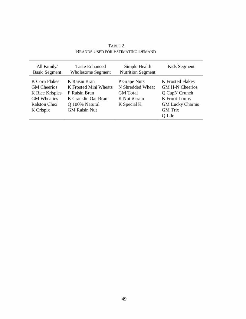
49

TABLE 2BRANDS USED FOR ESTIMATING DEMAND

All Family/Basic Segment

Taste EnhancedWholesome Segment

Simple HealthNutrition Segment

Kids Segment

K Corn FlakesGM CheeriosK Rice KrispiesGM WheatiesRalston ChexK Crispix

K Raisin BranK Frosted Mini WheatsP Raisin BranK Cracklin Oat BranQ 100% NaturalGM Raisin Nut

P Grape NutsN Shredded WheatGM TotalK NutriGrainK Special K

K Frosted FlakesGM H-N CheeriosQ CapN CrunchK Froot LoopsGM Lucky CharmsGM TrixQ Life

50

TABLE 3

RESULTS FROM LOGIT DEMAND(21,600 OBSERVATIONS)

OLS IV

Variable (i) (ii) (iii) (iv) (v) (vi)

Price -8.57(0.179)

-12.60(0.436)

-12.65(0.467)

-16.61(0.443)

-16.97(0.483)

-18.21(0.439)

Advertising 0.034(0.002)

0.032(0.002)

0.032(0.002)

0.030(0.002)

0.030(0.002)

0.030(0.002)

log median income -- -- -- 0.99(0.021)

1.00(0.022)

1.01(0.022)

log of median age -- -- -- -0.02(0.06)

0.01(0.06)

0.04(0.06)

median HH size -- -- -- -0.03(0.03)

-0.02(0.03)

-0.02(0.03)

Measures of fit:a 0.76 99.1(30.1)

98.7(16.9)

59.0(30.1)

51.3(16.9)

54.8(42.6)

First Stage:

R2 -- 94.5 94.4 94.5 94.5 94.7

F-statistic -- 5179 6740 5046 6483 4959

Instruments:

Avg regional prices -- T -- T -- T

Cost proxies

Own PriceElasticity:

-- -- T -- T T

Mean -1.71 -2.51 -2.51 -3.31 -3.38 -3.62

Std. 0.51 0.75 0.75 0.99 1.01 1.09

Median -1.60 -2.36 -2.36 -3.11 -3.18 -3.41

% of InelasticDemands (+/- 2 s.e.’s)

4.4%(4.1-4.9%)

0 0 0 0 0

Dependant variable is ln(Sjt)-ln(S0t). All regressions include time and brand dummy variables, robust standard errorsare given in parenthesis.aAdjusted R2 for the OLS regression, and a test of over identification for the IV regressions (Hausman, 1983) withthe 0.95 critical values in parenthesis.

51

TABLE 4OWN AND CROSS PRICE ELASTICITIES IMPLIED BY LOGIT DEMAND

own-price elasticity cross-price elasticitya

K Corn FlakesK Raisin BranK Frosted FlakesK Rice KrispiesK Frosted Mini WheatsK Froot LoopsK Special KK NutriGrainK CrispixK Cracklin Oat BranGM CheeriosGM Honey Nut CheeriosGM WheatiesGM TotalGM Lucky CharmsGM TrixGM Raisin NutP Raisin BranP Grape NutsQ 100% NaturalQ LifeQ Cap N CrunchChexN Shredded Wheat

-1.61-2.89-2.48-2.23-4.59-2.92-3.35-2.99-3.24-6.01-2.99-2.79-2.44-3.50-3.16-3.72-5.15-2.94-3.84-4.22-2.61-2.34-3.22-3.83

0.0340.0330.0470.0340.0240.0240.0160.0110.0120.0150.0510.0360.0140.0330.0210.0160.0120.0160.0210.0080.0120.0290.0100.013

aGives the percent change in market share of brand j with a one percent change in price of i, where i indexes rowand jûi. The Logit functional form implies that these elasticities are equa l for all jûi.

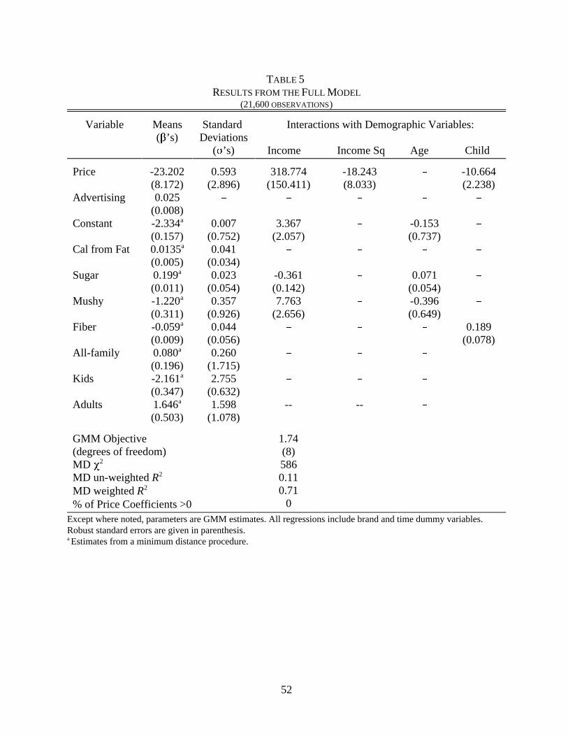
52

TABLE 5

RESULTS FROM THE FULL MODEL(21,600 OBSERVATIONS)

Variable Means($’s)

Standard Deviations

(F’s)

Interactions with Demographic Variables:

Income Income Sq Age Child

Price

Advertising

Constant

Cal from Fat

Sugar

Mushy

Fiber

All-family

Kids

Adults

-23.202(8.172)0.025

(0.008)-2.334a

(0.157)0.0135a

(0.005)0.199a

(0.011)-1.220a

(0.311)-0.059a

(0.009)0.080a

(0.196)-2.161a

(0.347)1.646a

(0.503)

0.593(2.896)

%

0.007(0.752)0.041

(0.034)0.023

(0.054)0.357

(0.926)0.044

(0.056)0.260

(1.715)2.755

(0.632)1.598

(1.078)

318.774(150.411)

%

3.367(2.057)

%

-0.361(0.142)7.763

(2.656)%

%

%

--

-18.243(8.033)

%

%

%

%

%

%

%

%

--

%

%

-0.153(0.737)

%

0.071(0.054)-0.396(0.649)

%

%

%

%

-10.664(2.238)

%

%

%

%

%

0.189(0.078)

GMM Objective (degrees of freedom)MD P2

MD un-weighted R2 MD weighted R2 % of Price Coefficients >0

1.74(8)5860.110.71

0Except where noted, parameters are GMM estimates. All regressions include brand and time dummy variables.Robust standard errors are given in parenthesis.a Estimates from a minimum distance procedure.

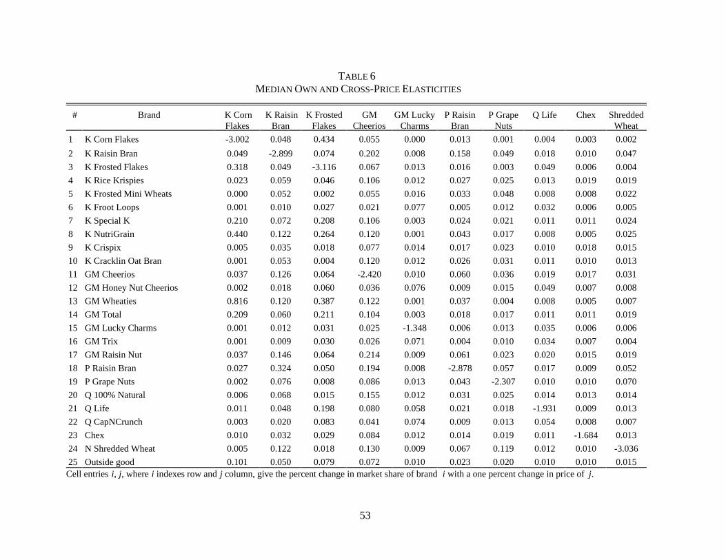
53

TABLE 6 MEDIAN OWN AND CROSS-PRICE ELASTICITIES

# Brand K CornFlakes

K RaisinBran

K FrostedFlakes

GMCheerios

GM LuckyCharms

P RaisinBran

P GrapeNuts

Q Life Chex ShreddedWheat

1 K Corn Flakes -3.002 0.048 0.434 0.055 0.000 0.013 0.001 0.004 0.003 0.002

2 K Raisin Bran 0.049 -2.899 0.074 0.202 0.008 0.158 0.049 0.018 0.010 0.047

3 K Frosted Flakes 0.318 0.049 -3.116 0.067 0.013 0.016 0.003 0.049 0.006 0.004

4 K Rice Krispies 0.023 0.059 0.046 0.106 0.012 0.027 0.025 0.013 0.019 0.019

5 K Frosted Mini Wheats 0.000 0.052 0.002 0.055 0.016 0.033 0.048 0.008 0.008 0.022

6 K Froot Loops 0.001 0.010 0.027 0.021 0.077 0.005 0.012 0.032 0.006 0.005

7 K Special K 0.210 0.072 0.208 0.106 0.003 0.024 0.021 0.011 0.011 0.024

8 K NutriGrain 0.440 0.122 0.264 0.120 0.001 0.043 0.017 0.008 0.005 0.025

9 K Crispix 0.005 0.035 0.018 0.077 0.014 0.017 0.023 0.010 0.018 0.015

10 K Cracklin Oat Bran 0.001 0.053 0.004 0.120 0.012 0.026 0.031 0.011 0.010 0.013

11 GM Cheerios 0.037 0.126 0.064 -2.420 0.010 0.060 0.036 0.019 0.017 0.031

12 GM Honey Nut Cheerios 0.002 0.018 0.060 0.036 0.076 0.009 0.015 0.049 0.007 0.008

13 GM Wheaties 0.816 0.120 0.387 0.122 0.001 0.037 0.004 0.008 0.005 0.007

14 GM Total 0.209 0.060 0.211 0.104 0.003 0.018 0.017 0.011 0.011 0.019

15 GM Lucky Charms 0.001 0.012 0.031 0.025 -1.348 0.006 0.013 0.035 0.006 0.006

16 GM Trix 0.001 0.009 0.030 0.026 0.071 0.004 0.010 0.034 0.007 0.004

17 GM Raisin Nut 0.037 0.146 0.064 0.214 0.009 0.061 0.023 0.020 0.015 0.019

18 P Raisin Bran 0.027 0.324 0.050 0.194 0.008 -2.878 0.057 0.017 0.009 0.052

19 P Grape Nuts 0.002 0.076 0.008 0.086 0.013 0.043 -2.307 0.010 0.010 0.070

20 Q 100% Natural 0.006 0.068 0.015 0.155 0.012 0.031 0.025 0.014 0.013 0.014

21 Q Life 0.011 0.048 0.198 0.080 0.058 0.021 0.018 -1.931 0.009 0.013

22 Q CapNCrunch 0.003 0.020 0.083 0.041 0.074 0.009 0.013 0.054 0.008 0.007

23 Chex 0.010 0.032 0.029 0.084 0.012 0.014 0.019 0.011 -1.684 0.013

24 N Shredded Wheat 0.005 0.122 0.018 0.130 0.009 0.067 0.119 0.012 0.010 -3.036

25 Outside good 0.101 0.050 0.079 0.072 0.010 0.023 0.020 0.010 0.010 0.015Cell entries i, j, where i indexes row and j column, give the percent change in market share of brand i with a one percent change in price of j.

54

TABLE 7PREDICTED MARGINAL COSTS

median pre-mergerprice

(¢ per serving)

median marginal cost(¢ per serving)

median margin

(p-mc)/p

Logit Full Model Logit Full Model

K Corn FlakesK Raisin BranK Frosted FlakesK Rice KrispiesK Frosted Mini WheatsK Froot LoopsK Special KK NutriGrainK CrispixK Cracklin Oat BranGM CheeriosGM Honey Nut CheeriosGM WheatiesGM TotalGM Lucky CharmsGM TrixGM Raisin NutP Raisin BranP Grape NutsQ 100% NaturalQ LifeQ Cap N CrunchChexN Shredded Wheat

9.817.214.813.128.018.320.618.019.337.018.817.415.622.220.223.032.817.823.626.115.614.919.727.5

3.110.78.36.5

21.411.714.111.412.630.312.511.09.3

15.813.816.726.411.717.519.99.58.7

13.621.5

5.59.88.62.6

14.82.9

15.212.55.2

22.510.13.1

12.517.12.85.1

24.711.214.014.96.43.48.0

18.8

68.5%38.1%44.2%50.4%23.7%36.4%31.7%36.4%34.3%18.0%34.0%36.7%40.9%28.7%31.8%27.8%19.6%34.3%25.8%23.6%39.2%41.2%30.7%21.9%

43.4%43.2%41.6%79.9%47.0%84.1%26.4%30.6%73.1%39.2%46.4%81.9%20.2%22.9%86.2%77.7%24.7%36.8%40.8%42.8%58.8%77.4%59.4%31.8%

55

TABLE 8PERCENT INCREASE IN PRICES AS A RESULT OF THE POST-NABISCO MERGER

pre-mergerprice

(¢ per serving)

Logit Full Model

approx approx new equilibrium cost reduction

K Corn FlakesK Raisin BranK Frosted FlakesK Rice KrispiesK Frosted Mini WheatsK Fruit Loops K Special KK NutriGrainK CrispixK Cracklin Oat BranGM CheeriosGM HN Cheerios GM WheatiesGM Total GM Lucky Charms GM TrixGM Raisin NutP Raisin BranP Grape NutsQ 100% NaturalQ LifeQ Cap N Crunch R ChexN Shredded Wheat

9.817.314.813.128.018.320.718.019.337.018.817.415.622.220.223.032.817.823.626.115.614.919.727.5

----------------------------------

0.10.1

--------

0.2

----------------------------------

0.61.2

--------

2.2

0.00.00.00.00.00.00.00.00.00.00.00.00.00.00.00.00.00.61.40.00.00.00.02.8

-0.0-0.1-0.00.00.00.0

-0.0-0.00.0

-0.00.00.0

-0.0-0.00.00.0

-0.0-3.0-1.80.00.00.00.0

-1.3The columns labeled approx refer to the prices that result from computing the prices using the approximation givenin equation (11) Since nothing changes for the non-merging firms the price increase will always be zero, andtherefore is not displayed. The column labeled “new equilibrium” computes the new Nash-Bertrand equilibriumand the column labeled “cost reduction” does the same but assumes a 5% reduction in marginal costs for all brandsof merging firms.

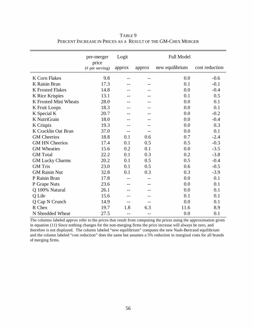
56

TABLE 9PERCENT INCREASE IN PRICES AS A RESULT OF THE GM-CHEX MERGER

pre-mergerprice

(¢ per serving)

Logit Full Model

approx approx new equilibrium cost reduction

K Corn FlakesK Raisin BranK Frosted FlakesK Rice KrispiesK Frosted Mini WheatsK Fruit Loops K Special KK NutriGrainK CrispixK Cracklin Oat BranGM CheeriosGM HN Cheerios GM WheatiesGM Total GM Lucky Charms GM TrixGM Raisin NutP Raisin BranP Grape NutsQ 100% NaturalQ LifeQ Cap N Crunch R ChexN Shredded Wheat

9.817.314.813.128.018.320.718.019.337.018.817.415.622.220.223.032.817.823.626.115.614.919.727.5

--------------------

0.10.10.20.10.10.10.1

----------

1.8--

--------------------

0.60.50.10.30.50.50.3

----------

6.3--

0.00.10.00.10.00.00.00.00.00.00.70.50.00.20.50.60.30.00.00.00.10.0

11.60.0

-0.6-0.1-0.40.50.10.1

-0.2-0.40.30.1

-2.4-0.3-3.5-3.8-0.4-0.5-3.90.10.10.10.10.18.90.1

The columns labeled approx refer to the prices that result from computing the prices using the approximation givenin equation (11) Since nothing changes for the non-merging firms the price increase will always be zero, andtherefore is not displayed. The column labeled “new equilibrium” computes the new Nash-Bertrand equilibriumand the column labeled “cost reduction” does the same but assumes a 5% reduction in marginal costs for all brandsof merging firms.

57

TABLE 10PERCENT INCREASE IN PRICES AS A RESULT OF THE KELLOGG-QUAKER OATS MERGER

pre-mergerprice

(¢ per serving)

Logit Full Model

approx approx new equilibrium cost reduction

K Corn FlakesK Raisin BranK Frosted FlakesK Rice KrispiesK Frosted Mini WheatsK Fruit Loops K Special KK NutriGrainK CrispixK Cracklin Oat BranGM CheeriosGM HN Cheerios GM WheatiesGM Total GM Lucky Charms GM TrixGM Raisin NutP Raisin BranP Grape NutsQ 100% NaturalQ LifeQ Cap N Crunch R ChexN Shredded Wheat

9.817.314.813.128.018.320.718.019.337.018.817.415.622.220.223.032.817.823.626.115.614.919.727.5

1.30.80.81.00.50.70.60.70.70.4

------------------

2.33.94.0

----

1.12.23.13.21.8

11.30.90.82.83.2

------------------

8.816.516.4

----

0.00.91.54.01.7

13.60.30.13.33.60.31.00.10.10.90.70.20.10.0

10.615.718.9-0.20.0

-0.7-1.3-0.24.0

-1.912.1-2.8-2.42.4

-0.30.30.90.00.10.80.60.20.10.07.9

14.919.1-0.10.0

The columns labeled approx refer to the prices that result from computing the prices using the approximation givenin equation (11) Since nothing changes for the non-merging firms the price increase will always be zero, andtherefore is not displayed. The column labeled “new equilibrium” computes the new Nash-Bertrand equilibriumand the column labeled “cost reduction” does the same but assumes a 5% reduction in marginal costs for all brandsof merging firms.

58

TABLE 11PERCENT INCREASE IN PRICES AS A RESULT OF THE GM-QUAKER OATS MERGER

pre-mergerprice

(¢ per serving)

Logit Full Model

approx approx new equilibrium cost reduction

K Corn FlakesK Raisin BranK Frosted FlakesK Rice KrispiesK Frosted Mini WheatsK Fruit Loops K Special KK NutriGrainK CrispixK Cracklin Oat BranGM CheeriosGM HN Cheerios GM WheatiesGM Total GM Lucky Charms GM TrixGM Raisin NutP Raisin BranP Grape NutsQ 100% NaturalQ LifeQ Cap N Crunch R ChexN Shredded Wheat

9.817.314.813.128.018.320.718.019.337.018.817.415.622.220.223.032.817.823.626.115.614.919.727.5

--------------------

0.60.70.70.50.60.50.4

----

1.52.42.4

----

--------------------

3.315.30.50.9

12.511.92.4

----

9.124.727.2

----

0.10.40.70.40.10.60.20.10.00.22.7

15.00.10.3

12.713.22.00.10.0

11.722.735.1-0.20.0

-0.50.30.20.80.10.5

-0.1-0.30.20.2

-0.415.2-3.4-3.412.211.2-2.40.20.08.2

20.934.60.10.1

The columns labeled approx refer to the prices that result from computing the prices using the approximation givenin equation (11) Since nothing changes for the non-merging firms the price increase will always be zero, andtherefore is not displayed. The column labeled “new equilibrium” computes the new Nash-Bertrand equilibriumand the column labeled “cost reduction” does the same but assumes a 5% reduction in marginal costs for all brandsof merging firms.

59

TABLE 12CHANGE IN PROFITS AND CONSUMER SURPLUS AS A RESULT OF A MERGER

Post &

Nabisco

General Mills &

Chex

General Mills&

Quaker Oats

Kellogg &

Quaker Oats

Consumer Surplus -10.86 -35.82 -222.25 -416.70

Profits (total) Kellogg General Mills Post Quaker Oats Ralston Nabisco

5.042.461.630.470.400.09

–

8.404.511.450.591.64

–0.18

90.3026.6256.614.51

–1.391.18

158.4872.9374.996.32

–2.321.92

Total Welfare -5.82 -27.42 -131.95 -258.22

with 5% reduction in mc:

Consumer Surplus 8.64 20.54 -176.68 -357.52

Profits (total) Kellogg General Mills Post Quaker Oats Ralston Nabisco

20.552.461.63

15.980.400.09

–

57.694.51

50.780.591.64

–0.18

150.4686.7756.614.51

–1.391.18

209.5572.93

126.076.32

–2.321.92

Total Welfare 29.24 78.23 -26.22 -147.97All computations are based on results of Tables 8-11.