Merit functions: a bridge between optimization and

equilibria

Massimo Pappalardo∗ Giandomenico Mastroeni∗ Mauro Passacantando∗

Abstract. In the last decades, many problems involving equilibria, arising from engineering,

physics and economics, have been formulated as variational mathematical models. In turn, these

models can be reformulated as optimization problems through merit functions. This paper aims

at reviewing the literature about merit functions for variational inequalities, quasi-variational

inequalities and abstract equilibrium problems. Smoothness and convexity properties of merit

functions and solution methods based on them will be presented.

Keywords. Merit functions, gap functions, variational inequalities, equilibrium problems,

descent methods.

1 Introduction

Optimization is a widespread mathematical technique in many engineering and economic appli-

cations. However, in many real-world problems, an objective function to be optimized is missing

and the concept of equilibrium becomes crucial. Roughly speaking, if optimization takes care

of the system utility function, the equilibrium takes into account the mutual interaction be-

tween users. In recent years, the interest in equilibrium problems has widely grown. The main

applications are concerned with traffic over telecommunication networks or over public roads,

oligopolistic and spatial price markets, financial markets, risk management, climate competition,

migration problems, power allocation in radio systems, internet advertising, cloud computing

(see e.g. [3, 5, 6, 13, 16, 24, 28, 34, 36, 48, 49, 50, 54, 66, 68, 70, 71, 80, 76, 88, 95, 102] and

references therein).

All these problems have been formulated in the literature through variational mathematical

models as complementarity problems, variational inequalities, quasi-variational inequalities, and

Nash equilibrium problems among others. Variational inequalities (VIs) are one of the most

known variational models. They were introduced by Hartman and Stampacchia [44] as a tool

for studying partial differential equations in infinite dimensional spaces arising from mechanics

(free-obstacle problem, friction problem, etc.). Later, their applications to contact problems in

mechanical structures provided a vaste source of finite dimensional problems.

A finite-dimensional VI is defined as follows:

find x∗ ∈ C such that 〈F (x∗), y − x∗〉 ≥ 0, for all y ∈ C, (VI)

∗Dipartimento di Informatica, Universita di Pisa, Largo B. Pontecorvo 3, 56127 Pisa, Italy.

1

where F : Rn → Rn, C is a closed and convex subset of Rn and 〈·, ·〉 is the scalar product in Rn.

Several kinds of numerical methods to solve VIs have been proposed (see, e.g., [33, 42] and ref-

erences therein). One popular approach is based on the reformulation of (VI) as an optimization

problem through suitable merit functions.

A function p : Rn → R is called merit function for (VI) if there exists a set Ω ⊆ Rn such

that:

• p is nonnegative on Ω,

• x∗ is a solution to (VI) if and only if x∗ ∈ Ω and p(x∗) = 0.

If the set Ω coincides with the feasible set C of (VI), a merit function is also known in the

literature as a gap function. Therefore, merit functions are the key concept to build a bridge

between VIs and optimization.

In this paper we aim at reviewing the state of the art concerning the merit function approach

for VIs and two interesting generalization of VIs: quasi-variational inequalities and abstract

equilibrium problems.

The rest of paper is organized as follows: Section 2 is devoted to the preliminary concepts that

will be used in the paper. Sections 3 deals with both constrained and unconstrained optimization

reformulations of (VI). In particular, we will describe continuity and differentiability properties

of merit functions, conditions under which merit functions are convex or their stationary points

solve (VI), and error bound results, i.e., how the distance between an arbitrary point x and the

solution set of (VI) can be estimated in terms of the merit function value at x. Furthermore, ad-

hoc descent methods for minimizing merit functions will be shown. Section 4 and 5 are devoted

to the results about merit functions for quasi-variational inequalities and abstract equilibrium

problems, respectively. Examples of applications of the presented models are provided in Sections

3, 4 and 5. Some concluding remarks and suggestions for future research are collected in Section

6. We hope that this paper may stimulate further interest in merit functions and may be the

basis to obtain new results.

2 Preliminaries

In this section, we show two particular cases of (VI), and we recall the main definitions and

preliminary results that will be used throughout the paper. We make the blanket assumptions

that the feasible set C of (VI) is closed and convex and the operator F is continuous on C.

Optimality conditions. As first particular case, let us consider the problem of finding a

local minimum x∗ of a differentiable function ψ : Rn → R over the set C. The classic first order

necessary optimality condition states that the directional derivative of ψ at x∗ in any feasible

direction is nonnegative, i.e.

〈∇ψ(x∗), y − x∗〉 ≥ 0, ∀ y ∈ C.

This condition is a particular case of (VI) where F (x) = ∇ψ(x).

Complementarity problems. Another example of (VI) is provided by a complementarity

problem described as follows: given a closed convex cone C ⊆ Rn and a mapping F : Rn → Rn,

the complementarity problem asks to determine a point x∗ ∈ C such that

〈F (x∗), x∗〉 = 0 and F (x∗) ∈ C∗,

2

where C∗ denotes the dual cone of C, i.e.

C∗ := d ∈ Rn : 〈d, y〉 ≥ 0 for all y ∈ C.

Solving the complementarity problem amounts to solving (VI). In fact, if x∗ solves the comple-

mentarity problem, then for any y ∈ C we have

〈F (x∗), y − x∗〉 = 〈F (x∗), y〉 ≥ 0,

hence x∗ solves (VI); vice versa, if x∗ solves (VI), then setting y = 0 and y = 2x∗ (which belong

to C because C is a cone) we obtain 〈F (x∗), x∗〉 = 0 and hence F (x∗) ∈ C∗, that is x∗ is a

solution to the complementarity problem. Note that if we define

p(x) := 〈F (x), x〉, Ω := x ∈ C : F (x) ∈ C∗, (1)

then p(x) ≥ 0 for any x ∈ Ω and x∗ solves the complementarity problem if and only if x∗ ∈ Ω

and p(x∗) = 0, i.e. p is a merit function for the complementarity problem.

Monotonicity definitions. Monotonicity is a key assumption to establish existence of

solutions, convergence results for algorithms and to provide error bounds for (VI). We now recall

the main monotonicity properties that will be exploited in the paper. F is said monotone on C

if

〈F (x)− F (y), x− y〉 ≥ 0, ∀ x, y ∈ C;

the corresponding concept of strict monotonicity is analogously defined just requiring strict

inequality to hold for any x, y ∈ C with x 6= y; F is said strongly monotone on C with modulus

µ if

〈F (x)− F (y), x− y〉 ≥ µ‖x− y‖2, ∀ x, y ∈ C,

for some µ > 0; F is said pseudomonotone on C if for any x, y ∈ C one has

〈F (y), x− y〉 ≥ 0 =⇒ 〈F (x), x− y〉 ≥ 0.

In the particular case where F (x) = ∇ψ(x), monotonicity and strong monotonicity of F on

C are equivalent to convexity and strong convexity of ψ on C, respectively.

Existence results. We now recall two basic results concerning the existence of a solution

to (VI). For the sake of simplicity, we will not consider the sharpest possible assumptions. The

solution set of (VI) is nonempty if either the feasible set C is bounded [44] or the following

coercivity condition holds: there exists a point y ∈ C such that

lim‖x‖→∞,x∈C

〈F (x), y − x〉 = −∞. (2)

In particular, condition (2) holds if F is strongly monotone on C. Moreover, the strong mono-

tonicity of F ensures that (VI) has a unique solution.

Fixed point problem reformulation. If we denote by πC the Euclidean projection oper-

ator on C, i.e.,

πC(x) := arg miny∈C‖y − x‖,

then it is well-known that (VI) is equivalent to finding a fixed point of the operator x 7→ πC(x−F (x)).

3

Complementarity problem reformulation. Assuming

C := x ∈ Rn : gi(x) ≤ 0, i = 1, . . . ,m, (3)

where the functions gi are differentiable and convex for all i = 1, . . . ,m, it is possible to derive

the Karush-Kuhn-Tucker (KKT) conditions for (VI). In fact, x∗ is a solution to (VI) if and only

if it is a global minimum of the following convex optimization problem:

miny∈C〈F (x∗), y〉.

Under some constraint qualification, the following KKT conditionsF (x∗) +

m∑i=1

λ∗i∇gi(x∗) = 0,

λ∗i gi(x∗) = 0, i = 1, . . . ,m,

λ∗i ≥ 0, gi(x∗) ≤ 0, i = 1, . . . ,m,

(4)

are necessary and sufficient for optimality and, in turn, for the existence of solutions to (VI). It

is well-known that KKT system (4) is equivalent to a complementarity problem.

3 Merit functions for variational inequalities

In this section we summarize several approaches in order to express (VI) as a constrained or

unconstrained optimization problem by means of different merit functions.

A first merit function can be defined by exploiting the fixed point reformulation stated in

Section 2. In fact, the function x 7→ ‖x− πC(x− F (x))‖ is a gap function for (VI) [29].

A further merit function for (VI) can be obtained by means of the complementarity refor-

mulation (4), which in turn can be associated with the merit function (1). Further examples of

merit functions associated with a complementarity problem can be found in [35].

3.1 Constrained optimization reformulations

This section is devoted to gap functions for (VI).

3.1.1 Auslender gap function

A first example of gap function was given in [8], where the following function was introduced:

p(x) := supy∈C〈F (x), x− y〉. (5)

It is trivial to prove that p is a gap function for (VI). Since the supremum in (5) can be infinite

or not attained in a unique point, this function is in general neither finite, nor differentiable,

nor convex. However, when C is bounded and F is continuously differentiable, it is finite and

admits directional derivatives p′(x; d) at any point x ∈ C in any direction d. Moreover, if F is

monotone, any stationary point x∗ of p on C, i.e.

p′(x∗; y − x∗) ≥ 0, ∀ y ∈ C,

4

is a solution to (VI). In the particular case of monotone affine VIs, i.e. if F (x) = Ax+ b where

A is a positive semidefinite matrix, p also turns out to be convex [58]. If F is strongly monotone

with modulus µ and x∗ is the unique solution to (VI), then p provides the following error bound:

‖x− x∗‖ ≤√p(x)/µ, ∀ x ∈ C.

A descent method based on the function p has been proposed in [61] in the case where C

is a bounded polyhedron. At each iteration, the descent direction is obtained by minimizing

a linearization of a further gap function. If F is monotone, then the algorithm is globally

convergent1 to a solution to (VI). Moreover, the convergence is quadratic2 if F is strongly

monotone and the termination is achieved in a finite number of iterations if F is affine. Under

a so-called “geometric stability condition”, it is shown that p also provides an error bound for

(VI).

3.1.2 Regularized gap functions

Many efforts of the research have been directed to the study of differentiable gap functions in

order to simplify the computational aspects of the problem. Important results in this sense have

been obtained in [37, 53, 96, 104].

First, Auchmuty [7] proposed a scheme in order to define a general class of gap functions:

pA(x) := supy∈C

[〈F (x), x− y〉+ f(x)− f(y)− 〈∇f(x), x− y〉] , (6)

where f : Rn → R is convex and continuously differentiable. It was proved that if (x∗, y∗) is a

saddle point of the function

L(x, y) := 〈F (x), x− y〉+ f(x)− f(y)− 〈∇f(x), x− y〉

on C × C, i.e.,

L(x∗, y) ≤ L(x∗, y∗) ≤ L(x, y∗), ∀ (x, y) ∈ C × C,

then x∗ is a solution to (VI) and pA is a gap function. We observe that if f is strongly convex

on C and F is differentiable, then the function pA is finite and differentiable.

Later, Fukushima [37] introduced a gap function which is a special case of (6), setting f(x) =

〈x,Mx〉/2, where M is a symmetric and positive definite matrix. It is defined by

pF (x) := maxy∈C

[〈F (x), x− y〉 − 1

2〈x− y,M (x− y)〉

]. (7)

Note that the maximum in (7) is always attained in a unique point y(x) since the objective

function is strongly concave with respect to the variable y, hence pF is always finite. If F is

continuously differentiable, then Danskin’s theorem [25] guarantees that also pF is so and

∇pF (x) = F (x)− [(∇F (x))T −M ](y(x)− x).

1The convergence is said global if it does not depend on the choice of the starting point.2A sequence xk is said to be convergent to x with rate of convergence equal to r if

lim supk→+∞

‖xk+1 − x‖‖xk − x‖r

= γ ∈ (0,+∞).

If r = 1 and γ ∈ (0, 1), then the convergence is said to be linear, if r > 1, then the convergence is said to be

superlinear, and, in particular, if r = 2, the convergence is said to be quadratic.

5

Moreover, if x∗ is a stationary point of pF on C, i.e.

〈∇pF (x∗), y − x∗〉 ≥ 0, ∀ y ∈ C,

and the Jacobian matrix ∇F (x∗) is positive definite, then x∗ is a solution to (VI). In the special

case of strongly monotone affine VIs, i.e. F (x) = Ax + b with A positive definite, pF turns out

to be convex (strongly convex) provided that the matrix A + AT −M is positive semidefinite

(positive definite) [53].

A descent algorithm for minimizing pF has been proposed in [37]: given any starting point

x0 ∈ C, the sequence xk is generated by the iterations

xk+1 = xk + tkdk, (8)

where the search direction dk = y(xk)− xk and the stepsize tk ∈ (0, 1] is such that

pF (xk + tkdk) = min

t∈(0,1]pF (xk + tdk). (9)

Under the assumptions that C is bounded, F is continuously differentiable on C and ∇F (x)

is positive definite for all x ∈ C, the sequence xk belongs to C and converges to the unique

solution to (VI). This algorithm converges also employing an inexact line search rule, provided

that F is strongly monotone on C and ∇F is Lipschitz continuous on C.

A variant of the above method which does not require the strong monotonicity of F has

been proposed in [103], setting the matrix M = αI, where I is the identity matrix. In fact, the

monotonicity of F paired with the boundedness of C guarantees that at any point x ∈ C the

vector y(x)− x, which depends on the matrix M and hence depends on α, is a descent direction

for pF , provided that α is small enough. The method performs a line search at the current iterate

xk if y(xk)− xk is a descent direction for pF ; otherwise the value of α is decreased. The method

is globally convergent if C is bounded and F is continuously differentiable and monotone on C.

This algorithm has been extended to nonsmooth VIs in [79].

In [60, 93] the authors propose a modified Newton method: at each iteration it finds the

solution to the linearized (VI) at x, i.e.

find z(x) s.t. 〈F (x) +∇F (x)[z(x)− x], y − z(x)〉 ≥ 0, ∀ y ∈ C. (10)

In the hypothesis of strong monotonicity of F , problem (10) admits a unique solution z(x) such

that d = z(x) − x is a descent direction for the gap functions pA and pF : the function pA has

been considered in [60], while pF in [93]. By employing a line search strategy, the method is

shown to be quadratically convergent under suitable additional assumptions.

When the feasible set C, defined as in (3), is not a polyhedron, the evaluation of the reg-

ularized gap function pF at a given point x could be computationally expensive. In order to

overcome this drawback, the following gap function has been proposed [92]:

pTF (x) := maxy∈T (x)

[〈F (x), x− y〉 − 1

2〈x− y,M(x− y)〉

], (11)

where

T (x) := y ∈ Rn : gi(x) + 〈∇gi(x), y − x〉 ≤ 0, i = 1, . . . ,m (12)

6

is an outer polyhedral approximation of C at x. If F is continuously differentiable, gi’s are

continuously differentiable and a constraint qualification holds, then pTF is directionally differ-

entiable. Furthermore, if ∇F is positive definite and gi’s are twice continuously differentiable,

then any stationary point of pTF on C is a solution to (VI). A successive quadratic programming

algorithm based on the minimization of an exact penalty function associated with pTF has been

proposed in [92].

A generalization of the gap function introduced by Fukushima has been proposed in [96, 104]

by replacing in (7) the regularizing term 〈x − y,M(x − y)〉/2 with a general bifunction G :

Rn × Rn → R such that:

G(x, y) ≥ 0 for all (x, y) ∈ Rn × Rn,G is continuously differentiable,

G(x, ·) is strongly convex on C for all x ∈ C,

G(x, x) = ∇yG(x, x) = 0 for all x ∈ C.

(13)

For any α > 0, the function

pα(x) := maxy∈C

[〈F (x), x− y〉 − αG(x, y)] (14)

turns out to be a gap function, which is continuously differentiable, if F is so, with

∇pα(x) = F (x)− (∇F (x))T (yα(x)− x)− α∇xG(x, yα(x)), (15)

where yα(x) is the unique solution to problem (14). Note that when F is only locally Lipschitz

continuous, the function pα is also locally Lipschitz and its Clarke generalized gradient satisfies

a formula similar to (15) (see [73]). Moreover, if x∗ is a stationary point of pα on C and ∇F (x∗)

is positive definite, then x∗ solves (VI). A further important feature of pα is that, under the

assumption that F is strongly monotone and ∇yG(x, ·) is Lipschitz continuous on C, for every

x ∈ C, it provides an error bound [104], i.e., there exists M > 0 such that

‖x− x∗‖ ≤M√pα(x), ∀ x ∈ C, (16)

where x∗ is the unique solution to (VI). In particular, (16) implies the boundedness of the sublevel

sets of pα, which is of crucial importance in the convergence of the minimization algorithms.

The descent methods developed in [37] have been generalized to a more general framework

exploiting several classes of gap functions defined by (14) (see [104]). Given a continuous mapping

Γ : C×C → Rn, such that Γ(x, ·) is strongly monotone on C for any x ∈ C, the following auxiliary

variational inequality is considered at a given point x ∈ C: find y∗ ∈ C such that

〈Γ(x, y∗)− Γ(x, x) + F (x), y − y∗〉 ≥ 0, ∀ y ∈ C. (AVI(x))

Having denoted by w(x) the unique solution to (AVI(x)), one can prove that the mapping

w : C → C is continuous and x∗ is a solution to (VI) if and only if x∗ = w(x∗). In view of this

result the following iterative method is proposed. Given xk ∈ C, compute w(xk): if w(xk) = xk,

then xk is a solution to (VI), otherwise find xk+1 performing an Armijo3 inexact line search for

the gap function pα along the direction dk := w(xk)− xk.

3The Armijo inexact line search along the direction dk consists in finding the smallest non negative integer m

such that

pα(xk + βmdk) ≤ pα(xk)− σ βm‖dk‖2,where β, σ ∈ (0, 1) are parameters, and then setting xk+1 := xk + βmdk.

7

Each combination of G and Γ generates a different descent algorithm, which is globally

convergent to the unique solution to (VI) under the assumption of continuous differentiability

and strong monotonicity of F and suitable additional assumptions on G and Γ [104]. Note that

the algorithm (8)–(9) previously described is recovered by setting Γ(x, y) = M(y − x).

The analysis of the convergence properties of the descent methods based on the regularized

gap functions pF and pα in the case where the operator F is nondifferentiable has been considered

in [72, 94].

3.1.3 Minty (dual) gap functions

The Minty (or dual) variational inequality was introduced in [67] and consists in finding x∗ ∈ Csuch that

〈F (y), y − x∗〉 ≥ 0, ∀ y ∈ C. (MVI)

Its relevance to applications was pointed out in [40, 77, 78]. In particular, Minty states the

equivalence between (VI) and (MVI) when F is pseudomonotone on C [67].

In parallel with the Auslender gap function, it can be shown that

pM (x) := supy∈C〈F (y), x− y〉 (17)

is a gap function for (MVI) and hence it is a gap function for (VI) provided that F is pseu-

domonotone on C.

The most important feature of this function, known in the literature as Minty (or dual) gap

function, is its convexity. However, it is in general nondifferentiable; subdifferentiability and

related properties have been analysed in [60, 62, 74, 97, 100]. Furthermore, it can be difficult to

evaluate pM since the optimization problem in (17) is generally not convex.

A cutting plane method for minimizing pM has been proposed in [74]: at each iteration it

solves a linear programming problem, provided that C is a polyhedron, and it converges to a

solution to (VI) if F is strictly monotone. Later, this method has been combined with the

Tikhonov regularization technique in order to deal with monotone VIs [15].

Following the scheme described before for (VI), it is possible to regularize the function pM

exploiting a bifunction G which satisfies conditions (13). In fact, the function

pMG (x) := supy∈C

[〈F (y), x− y〉 −G(x, y)] (18)

is a gap function for (MVI) (see [63]). Moreover, if the optimization problem in (18) has a unique

solution y(x), then pMG is continuously differentiable and its gradient is given by

∇pMG (x) = F (y(x))−∇xG(x, y(x)).

In parallel with the analysis developed for (VI), a descent method for the function pMG has been

proposed in [63]. Given any starting point x0 ∈ C, any sequence xk generated by an exact

line search algorithm with descent direction given by y(x)− x converges to the unique solution

to (VI), provided that C is compact, F is continuously differentiable, ∇F is positive definite on

C and

∇xG(x, y) +∇yG(x, y) = 0, ∀ x, y ∈ C.

8

Observe that the latter condition is fulfilled, for instance, by

G(x, y) =1

2〈x− y,M(x− y)〉.

This algorithm is stated in [64] employing an inexact linesearch rule and replacing the assumption

that ∇F (x) is positive definite for x ∈ C with the strong monotonicity of F on C.

A different regularization of the gap function pM has been proposed in [97], where the fol-

lowing function is considered:

pMβ (x) := supy∈C

[〈F (y), x− y〉+ β‖x− y‖2], (19)

where β is a positive parameter. This function is convex and lower semicontinuous as the original

pM . It is continuously differentiable provided that F is so and the supremum in (19) is attained

in a unique point. Moreover, if F is strongly monotone on C with modulus µ, and β ∈ (0, µ], it

is a gap function for (VI) and provides an error bound, i.e.

‖x− x∗‖ ≤√pMβ (x)/β, ∀ x ∈ C, (20)

where x∗ is the unique solution to (VI).

3.1.4 Gap functions based on conjugate duality

Given a convex function f : Rn → R and a concave function g : Rn → R, we recall that

f∗(y) := supx∈Rn

[〈y, x〉 − f(x)], g∗(y) := infx∈Rn

[〈y, x〉 − g(x)]

are the Fenchel conjugate, in convex and concave sense respectively, of f and g (see e.g. [87]).

Moreover, the Fenchel dual of the problem

infx∈Rn

[f(x)− g(x)]

is defined as

supy∈Rn

[g∗(y)− f∗(y)].

Note that the Fenchel dual of the constrained problem

infx∈C

f(x)

can be obtained defining g(x) = −δC(x), where δC is the indicator4 function of the set C, so

that

infx∈C

f(x) = infx∈Rn

[f(x)− (−δC(x))],

and the associated Fenchel dual turns out to be

supy∈Rn

[−f∗(y) + infx∈C〈y, x〉].

4δC is defined as follows: δC(x) = 0 if x ∈ C and δC(x) = +∞ otherwise.

9

When the feasible set C is explicitly defined by convex constraints as in (3), the value of the

Auslender gap function p at a given point x coincides (see [1, 53]) with the opposite of the optimal

value of the Fenchel dual of the problem

infy∈C〈F (x), y − x〉. (P (x))

Moreover, the opposite of the optimal value of the so called Lagrangian dual and the Fenchel-

Lagrange dual associated with P (x) leads to define a further gap function that coincides with

pL(x) := infλ≥0

supy∈Rn

[〈F (x), x− y〉 − 〈λ, g(y)〉], (21)

which has been proposed in [39].

Similarly, considering the opposite of the optimal values of the Lagrange and of the Fenchel

dual associated with the problem

infy∈C〈F (y), y − x〉,

which is equivalent to the one which appears in the right-hand side of (17), the following gap

functions for (MVI) are defined [1]:

pML(x) := infλ≥0

supy∈Rn

[〈F (y), x− y〉 − 〈λ, g(y)〉] , (22)

pMF (x) := infp∈Rn

supy∈Rn

[〈F (y), x− y〉+ 〈p, y〉] + δ∗C(−p), (23)

where δ∗C(x) = supy∈C〈x, y〉 is the support function to the set C.

The proposed gap functions are all convex if F is an affine monotone map.

3.2 Unconstrained optimization reformulations

In this section, we show merit functions which allow to reformulate (VI) as an unconstrained

optimization problem.

3.2.1 D-gap functions

The difference of two regularized gap functions

pαβ(x) := pα(x)− pβ(x), (24)

where pα and pβ are defined by (14) with 0 < α < β, is called D-gap function (where D stands

for “difference”). This function is nonnegative on the whole space Rn and pαβ(x∗) = 0 if and

only if x∗ is a solution to (VI) [98]. Therefore, solving (VI) is equivalent to finding the optimal

solutions of the problem

minx∈Rn

pαβ(x). (25)

When (VI) is a nonlinear complementarity problem, the D-gap function with β = 1/α and

α ∈ (0, 1) coincides with the implicit Lagrangian proposed and studied in [57, 81, 83].

10

Clearly, the D-gap function inherits the differentiability properties of pα and pβ , i.e., if F is

differentiable, the function pαβ is also differentiable and

∇pαβ(x) = (∇F (x))T [yβ(x)− yα(x)] + β∇xG(x, yβ(x))− α∇xG(x, yα(x)), (26)

where yα(x) and yβ(x) are the solutions of the optimization problem (14) with α and β respec-

tively. When the mapping F is locally Lipschitz continuous, the D-gap function is also locally

Lipschitz and the Clarke generalized gradient of pαβ satisfies a formula similar to (26) (see [72]).

The D-gap function is not convex in general and the stationary points of (25) may not be

global minima. However, if x∗ is a stationary point, i.e. ∇pαβ(x∗) = 0, and the Jacobian

matrix ∇F (x∗) is positive definite, then x∗ is a solution to (VI) [98]. Notice that the positive

definiteness of ∇F (x∗) can not be replaced by the strict monotonicity assumption on F (see the

counterexample in [98]). When the feasible set C is a box, it is sufficient to assume that ∇F (x∗)

is a P -matrix (i.e. its principal minors are all positive) to obtain the same conclusion [46]. In

the special case of strongly monotone affine VIs, the D-gap function is convex (strongly convex)

provided that the parameters α and β are chosen so that the matrix

A+AT − αI − β−1AT A (27)

is positive semidefinite (positive definite) [84].

Since the D-gap functions allow to reformulate (VI) as an unconstrained problem, the bound-

edness of their level sets is an important issue in order to develop minimization algorithms for

solving problem (25). The level sets of the D-gap function, denoted by

L(c) := x ∈ Rn : pαβ(x) ≤ c,

are bounded for all c ≥ 0 if either C is bounded [46] or F is strongly monotone [84, 85]. Recently,

it has been proved that monotonicity assumptions on F are not needed for the boundedness of

the level sets: in fact, the sets L(c) are bounded for all c ≥ 0 provided a coercivity condition

stronger than (2) holds [56].

If F is strongly monotone on Rn and either F is Lipschitz continuous on Rn or C is bounded,

then√pαβ provides an error bound for (VI), i.e. there exists a constant M > 0 such that

‖x− x∗‖ ≤M√pαβ(x), ∀ x ∈ Rn,

(see [98]). Notice that when C is unbounded, the strong monotonicity on F , without the Lipschitz

continuity assumption, is not sufficient to guarantee the same result (see the counterexample

in [45]). However, when F is strongly monotone, (VI) has a unique solution and hence it is

possible to reformulate the problem by replacing the set C by its intersection with a sphere large

enough to contain the solution. In the special case where C is a box, the strong monotonicity of

F can be replaced by the assumption that F is a uniform P -function [46]. Recently, new global

error bounds have been proposed in [55].

On the other hand, the strong monotonicity on F only guarantees a local error bound on the

level sets of the D-gap function [85], that is for any c ≥ 0 there exists M > 0 such that

‖x− x∗‖ ≤M√pαβ(x), ∀ x ∈ L(c).

11

Recently, this result has been extended to locally ξ-monotone and coercive mappings [55] and to

general nonmonotone mappings [56].

There are several solution methods for VIs based on the minimization of D-gap functions.

A descent method with Armijo-type line search has been proposed in [98]: at each itera-

tion it exploits the search direction d = r(x) + ρ s(x), where r(x) = yα(x) − yβ(x), s(x) =

α∇xG(x, yα(x)) − β∇xG(x, yβ(x)) and ρ > 0 is a sufficiently small constant. This method

converges to the solution to (VI) if F is strongly monotone on Rn and either F is Lipschitz

continuous on Rn or C is bounded. Another descent method was developed in [89] for solving

monotone VIs with bounded feasible set. It is similar to the method proposed in [103] based on

the Fukushima’s regularized gap function: at each iteration it uses d = yα(x)− yβ(x) as search

direction along with a suitable update of the parameters α and β. A descent method for solving

nonmonotone VIs, which is based on the minimization of the function√pαβ , has been presented

recently in [56].

A hybrid Newton method has been proposed in [84]: at each iteration, it finds the solution

z(x) of the linearized VI (10) at x and it tries to use the direction d = z(x) − x whenever it

provides a sufficient decrease in the D-gap function pαβ ; otherwise the direction d = −∇pαβ(x) is

used. Then, an inexact line search is performed to get the next iterate. The generated sequence

converges superlinearly to the unique solution x∗ to (VI) if F is continuously differentiable

and strongly monotone on Rn. Furthermore, the convergence is quadratic if ∇F is Lipschitz

continuous around x∗. A variant of this method has been proposed in [82] for box constrained

VIs.

In [46] a nonsmooth Gauss-Newton type method for solving box constrained VIs has been

presented. At each iteration, it solves a linear system of equations involving the generalized

Hessian of the D-gap function and tries to use this vector as search direction if a descent condition

is satisfied; otherwise the direction d = −∇pαβ(x) is used. Then an inexact line search is

performed. The algorithm is globally and superlinearly convergent under suitable assumptions.

A similar Gauss-Newton strategy has also been adopted in a trust region method for minimizing

the D-gap function [90].

Another Newton type method for the solution of box constrained VIs is based on the reformu-

lation of (VI) as a system of nonsmooth and nonlinear equations involving the natural residual.

This method, based on the minimization of D-gap function, is globally and superlinearly conver-

gent [47].

3.2.2 Merit functions via the Moreau-Yosida regularization

Another approach to get unconstrained optimization reformulations of (VI) is based on the

Moreau-Yosida regularization of some gap functions [97].

The function

pMYαλ (x) := inf

z∈C

supy∈C

[〈F (z), z − y〉 − α ‖y − z‖2

]+ λ ‖z − x‖2

, (28)

with α ≥ 0 and λ > 0, is derived from the Moreau-Yosida regularization of the regularized gap

function pF , with M = α I. It is nonnegative on the whole space Rn and pMYαλ (x∗) = 0 if and

only if x∗ solves (VI).

Notice that this merit function may not be easy to evaluate in practice unless (VI) has a

certain special structure (e.g. F is affine and C is a polyhedron [97]). However, it enjoys some

12

nice theoretical properties that other merit functions do not have. For instance, if the minimum

problem in (28) has a unique solution zαλ(x) for each x ∈ Rn, then pMYαλ is differentiable on Rn

and

∇pMYαλ (x) = 2λ [x− zαλ(x)],

even if F is not differentiable.

In general, the function pMYαλ is not convex. However, if the gap function p is convex, then

pMY0λ is differentiable and convex on Rn for any λ > 0; while if the regularized gap function pF ,

with M = α I, is convex then pMYαλ is differentiable and convex on Rn for any λ > 0.

The function pMYαλ provides also a global error bound under the strong monotonicity of F

(without assuming Lipschitz continuity as is the case for the D-gap functions). In fact, if F is

strongly monotone on C with modulus µ, α ∈ [0, µ) and λ > 0, then

1

2minµ− α, λ‖x− x∗‖2 ≤ pMY

αλ (x) ≤ λ ‖x− x∗‖2, ∀ x ∈ Rn,

i.e. the growth rate of pMYαλ is in the order of the squared distance from the unique solution x∗

to (VI).

When F satisfies suitable monotonicity assumptions, further merit functions for (VI) can be

obtained by the Moreau-Yosida regularization of Minty gap functions. The function

pMβλ(x) := infz∈C

supy∈C

[〈F (y), z − y〉+ β ‖y − z‖2

]+ λ ‖z − x‖2

, (29)

with β ≥ 0 and λ > 0, is the Moreau-Yosida regularization of Minty gap function pM (when

β = 0) and regularized Minty gap function pMβ (when β > 0). If F is pseudomonotone on C,

then pM0λ turns out to be a merit function for (VI) for any λ > 0, because it is nonnegative on

Rn and pM0λ(x∗) = 0 if and only if x∗ solves (VI). Furthermore, if F is strongly monotone with

modulus µ, then the same happens for pMβλ provided that β ∈ [0, µ].

Note that also pMβλ may not be easy to evaluate in practice, but some nice theoretical properties

hold. In fact, it is differentiable and convex on Rn for any β ≥ 0 and λ > 0, without making

any additional assumption on F . Moreover, if F is strongly monotone on C with modulus µ,

β ∈ (0, µ] and λ > 0, then the quadratic growth rate of pMβλ is ensured, i.e.

1

2minβ, λ‖x− x∗‖2 ≤ pMβλ(x) ≤ λ ‖x− x∗‖2, ∀ x ∈ Rn,

where x∗ is the unique solution to (VI).

3.3 An application to traffic network equilibrium problems

A traffic network consists of a set of nodes N, a set of arcs A ⊆ N × N and a set of ori-

gin/destination pairs W ⊆ N×N. For each O/D pair w, a traffic demand dw has to be distributed

among the paths connecting w. We denote Pw the set of all paths connecting w, xp the flow on

path p and x = (xp)p∈Pw,w∈W the vector of all path flows. The set of feasible path flows is given

by

X =

x ≥ 0 :∑p∈Pw

xp = dw, ∀ w ∈W

.

13

The flow fa on each arc a is the sum of all flows on paths to which the arc belongs, hence the arc

flow vector f = (fa)a∈A can be written as f = ∆x, where ∆ is the arc-path incidence matrix:

∆a,p =

1 if a ∈ p,0 otherwise.

For each arc a, there is a nonnegative cost function ta(f), which represents the travel time

associated with arc a and depends on the arc flow vector f . The corresponding path cost

function is assumed to be additive, i.e. the travel time Tp(x) on path p is the sum of the travel

times of the arcs belonging to p:

Tp(x) =∑a∈p

ta(∆x).

According to the Wardrop equilibrium principle [95], a path flow x∗ ∈ X is called a network

equilibrium if it is positive only on minimum cost paths, i.e. the following implication

x∗p > 0 =⇒ Tp(x∗) = min

q∈PwTq(x

∗)

holds for any O/D pair w ∈W and path p ∈ Pw.

It is well-known [24] that the problem of finding network equilibria is equivalent to solving

the following variational inequality:

find x∗ ∈ X such that 〈T (x∗), y − x∗〉 ≥ 0, for all y ∈ X. (30)

Next example shows how the merit function approach for VIs can be applied to network

equilibria.

Example 3.1. Consider the network in Fig. 1 with two O/D pairs: w1 = (1, 4) with de-

mand d1 = 4 and w2 = (1, 5) with d2 = 6. Each O/D pair is connected by two paths:

Pw1 = (1, 2), (2, 4); (1, 3), (3, 4) and Pw2 = (1, 2), (2, 5); (1, 3), (3, 5). We denote the flow on

paths as x1 . . . , x4, respectively. Hence the set of feasible path flows is given by

X = x ∈ R4+ : x1 + x2 = 4, x3 + x4 = 6.

Figure 1: Traffic network in Example 3.1.

14

Assume that the arc cost functions are defined as follows:

t12 := f12 + 1 = x1 + x3 + 1,

t13 := 3 f13 + 2 = 3 (x2 + x4) + 2,

t24 := 2 f24 + f34 + 1 = 2x1 + x2 + 1,

t25 := 2 f25 + f35 + 3 = 2x3 + x4 + 3,

t34 := f34 + 2 = x2 + 2,

t35 := 4 f35 + 1 = 4x4 + 1,

thus the corresponding path costs areT1 = t12 + t24 = 3x1 + x2 + x3 + 2,

T2 = t13 + t34 = 4x2 + 3x4 + 4,

T3 = t12 + t25 = x1 + 3x3 + x4 + 4,

T4 = t13 + t35 = 3x2 + 7x4 + 3,

i.e. the operator of VI (30) is T (x) = Ax+ b, with

A =

3 1 1 0

0 4 0 3

1 0 3 1

0 3 0 7

, b =

2

4

4

3

.

Note that the matrix A is positive definite, thus the mapping T is strongly monotone and there

exists a unique solution of VI (30), i.e. a unique network equilibrium.

We now consider the Fukushima’s regularized gap function (7) with M = I, i.e.

pF (x) = maxy∈X

[〈T (x), x− y〉 − 1

2‖x− y‖2

].

This function is continuously differentiable and strongly convex since the matrix A + AT − I is

positive definite. In Fig. 2 we show the graph of pF defined on the 2-dimensional space (x1, x3),

with x1 ∈ [0, 4] and x3 ∈ [0, 6] (the demand constraints allow to express variables x2 and x4 as

function of x1 and x3).

The descent algorithm (8)-(9) applied to pF can be exploited to compute the network equi-

librium. Table 1 reports the first four iterations of the algorithm (implemented in MATLAB)

starting from the feasible flow (4, 0, 6, 0).

Iteration x1 x2 x3 x4 pF (x)

0 4.000000 0 6.000000 0 1.5000 e+02

1 2.679622 1.320378 4.019434 1.980566 8.8840 e–03

2 2.631471 1.368529 4.052452 1.947548 1.5178 e–06

3 2.631587 1.368413 4.052626 1.947374 2.5929 e–10

4 2.631579 1.368421 4.052632 1.947368 2.8747 e–14

Table 1: Numerical results of the descent algorithm (8)-(9) applied to Example 3.1.

15

Figure 2: The regularized gap function pF with M = I in Example 3.1.

Note that the path costs corresponding to the equilibrium solution

x∗ = (2.6316, 1.3684, 4.0526, 1.9474)

are

T (x∗) = (15.3158, 15.3158, 20.7368, 20.7368),

i.e. the two paths connecting each O/D pair have the same cost. Furthermore, the Lagrange

multipliers λ∗ associated with x∗ in the KKT conditions (4) coincide with the equilibrium costs,

i.e. λ∗ = (15.3158, 20.7368).

Figure 3 shows the graph of the D-gap function pαβ, with α = 1, β = 2 and G(x, y) =

‖x− y‖2/2, defined on the space (x1, x3). Note that this function is always nonnegative (even in

unfeasible points) and its global minimum is x∗.

4 Merit functions for quasi-variational inequalities

In this section we consider the merit function approach for quasi-variational inequalities (QVIs),

i.e. VIs in which the feasible region depends on the variable x. Given a vector-valued mapping

F : Rn → Rn and a set-valued mapping C : Rn ⇒ Rn, such that C(x) are closed and convex sets

for any x ∈ Rn, the QVI is defined as follows:

find x∗ ∈ C(x∗) such that 〈F (x∗), y − x∗〉 ≥ 0, for all y ∈ C(x∗). (QVI)

16

Figure 3: The D-gap function pαβ with α = 1, β = 2 and G(x, y) = ‖x− y‖2/2 in Example 3.1.

17

When all the sets C(x) coincide with the same set C, (QVI) collapses to (VI). The set of fixed

points of the mapping C, i.e.

X := x ∈ Rn : x ∈ C(x),

is the feasible region of (QVI). In the following we suppose that sets C(x) are defined by con-

straints, i.e.,

C(x) := y ∈ Rn : gi(x, y) ≤ 0, i = 1, . . . ,m,

where the functions gi : Rn × Rn → R are assumed to be continuous and gi(x, ·) convex for any

fixed x ∈ Rn. Furthermore, in order to guarantee the convexity of the set X, we assume that

the functions x 7→ gi(x, x) are convex for all i = 1, . . . ,m.

QVIs were introduced in [11, 12] and subsequently exploited to model several finite and

infinite-dimensional problems (see [10, 22, 31, 32] and references therein).

Some merit functions have been proposed in the literature extending to QVIs similar ideas

developed for VIs. Similarly to VIs, the reformulation of (QVI) as a fixed point problem leads to

define a merit function. In fact, it follows from the definition that x solves (QVI) if and only if

x = πC(x)(x−F (x)), thus ‖x−πC(x)(x−F (x))‖ is a merit function for (QVI). Another approach

is based on reformulating (QVI), under suitable constraint qualifications, as a complementarity

problem via the following KKT conditions:F (x) +

m∑i=1

λi∇ygi(x, x) = 0,

λi gi(x, x) = 0, i = 1, . . . ,m,

λi ≥ 0, gi(x, x) ≤ 0, i = 1, . . . ,m.

Recently, a solution method based on these conditions has been proposed in [31].

A straightforward extension of the gap function (5) to QVIs is defined as follows [39]:

p(x) := supy∈C(x)

〈F (x), x− y〉. (31)

This function is nonnegative on the set X and x∗ solves (QVI) if and only if x∗ ∈ X and

p(x∗) = 0. However, the gap function p is nondifferentiable and it may occur that p(x) = +∞for some point of X.

The regularized gap function (7) has been extended to QVIs in [38] and is defined by

pα(x) := maxy∈C(x)

[〈F (x), x− y〉 − α

2‖x− y‖2

]. (32)

This function is a gap function, it is finite and the maximum in (32) is attained in a unique point

yα(x), provided that the set C(x) is nonempty. Actually, it is possible to define pα replacing

the regularization term α‖x − y‖2/2 and the set C(x) with more general expressions satisfying

suitable conditions [38, 91].

In contrast to VIs, this function is nondifferentiable even if F is so (see examples in [43]). If F

and gi are continuously differentiable and a constraint qualification holds, then pα is directionally

differentiable everywhere and its directional derivative at x along direction d is given by

p′α(x; d) = minλ∈Λα(x)

〈F (x)− [(∇F (x))T − α I][yα(x)− x]−m∑i=1

λi∇xgi(x, yα(x)), d〉,

18

where Λα(x) is the set of Lagrange multipliers associated with yα(x), i.e.,

Λα(x) = λ ∈ Rm+ : F (x) + α[yα(x)− x] +∑mi=1 λi∇ygi(x, yα(x)) = 0,

λi gi(x, yα(x)) = 0, i = 1, . . . ,m,

(see [38]). Furthermore, pα turns out to be continuously differentiable in the special case of

QVI with ‘moving sets’, i.e. when C(x) = Q + c(x), where Q is a closed and convex set and

c : Rn → Rn, provided that mappings F and c are continuously differentiable [27]. Recently, this

latter result has been extended to QVIs with generalized moving sets [43].

Similarly to VIs, the regularized gap function pα is nonconvex in general. In [91] it is proved

that, whenever pα is directionally differentiable, a stationary point x∗ of pα on X, i.e.

p′α(x∗; y − x∗) ≥ 0, ∀ y ∈ X,

is a solution to (QVI) provided that the matrix ∇F (x∗) is positive definite and

λi 〈∇xgi(x∗, yα(x∗)), yα(x∗)− x∗〉 ≥ 0

for all i = 1, . . . ,m and λ ∈ Λ(x). Notice that in [91] the key assumption yα(x∗) ∈ X is not

explicitly stated in the statement, but it is exploited in the proof and must be therefore considered

as hypothesis.

An unconstrained minimization reformulation of (QVI) can be obtained via the D-gap func-

tions, i.e. the difference of two regularized gap functions. In fact, given 0 < α < β, the function

pαβ(x) := pα(x)− pβ(x)

is nonnegative on Rn and pαβ(x∗) = 0 if and only if x∗ solves (QVI). The directional differentia-

bility of pαβ directly follows from that of pα and pβ .

The functions√pα and

√pαβ provide error bound results for (QVI) provided that F is

strongly monotone and Lipschitz continuous on Rn and an additional technical assumption on

the Euclidean projection on the sets C(x) is fulfilled [41]. Another error bound result based on

the function√pα has been recently proved in [9].

4.1 An application to generalized Nash equilibrium problems

Let us consider a noncooperative game with N players, in which each player i controls a set of

variables xi ∈ Rni . The vector of all players strategies is denoted by x = (x1, . . . , xN ) ∈ Rn, with

n = n1 + . . . , nN ; the vector x is also denoted by x = (xi, x−i), where x−i denotes the strategy

vector of all the players different from player i. Each player i has a cost function θi : Rn → R,

which possibly depends on all players strategies x, and a feasible set Xi(x−i) ⊆ Rni , possibly

depending on the rival players’ strategies x−i.

A generalized Nash equilibrium (GNE) of the game is a vector

x∗ = (x∗1, . . . , x∗N ) ∈ X1(x∗−1)× · · · ×XN (x∗−N )

such that, for any i = 1, . . . , N , x∗i is an optimal solution of the following optimization problem:

minxi

θi(xi, x∗−i) subject to xi ∈ Xi(x

∗−i).

19

In other words, x∗ is a GNE if no player can improve its own cost function by unilaterally

changing its strategy.

It is well-known (see e.g. [30]) that under the following assumptions:

• θi is continuously differentiable for any i = 1, . . . , N ,

• θi(·, x−i) is convex for any x−i and i = 1, . . . , N ,

• the feasible sets Xi(x−i) are closed and convex for all x ∈ Rn and i = 1, . . . , N ,

the problem of finding GNE is equivalent to solving the QVI with operator

F (x) = (∇x1θ1(x), . . . ,∇xN θN (x))

and set-valued mapping

C(x) = X1(x−1)× . . . XN (x−N ).

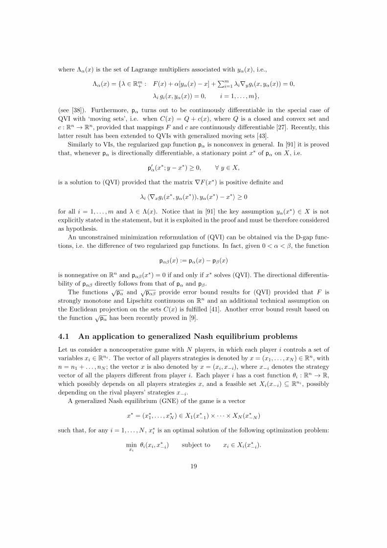
Example 4.1. (see [20]) Consider a two-person noncooperative game, in which player i select the

coordinate xi ∈ R subject to a individual constraint xi ≤ 0 and a shared constraint x1 +x2 ≤ −1.

The aim of player i is to minimize the (squared) distance between (x1, x2) and his favourite goal

Pi ∈ R2, with P1 = (1, 0) and P2 = (0, 1). Thus the optimization problems of the two players are

defined as follows:

Player 1:

minx1

(x1 − 1)2 + x22

x1 ≤ 0

x1 + x2 ≤ −1

Player 2:

minx2

x21 + (x2 − 1)2

x2 ≤ 0

x1 + x2 ≤ −1

The set of GNE of the game coincide with the solution set of the QVI given by F (x) = (2x1 −2, 2x2 − 2) and

C(x) = (−∞,min0,−1− x2]× (−∞,min0,−1− x1].

The feasible region of the QVI, i.e. the set of fixed point of the set-valued mapping C, is

X = x ∈ R2 : x1 ≤ 0, x2 ≤ 0, x1 + x2 ≤ −1.

It is easy to check that the solution set of the QVI is the segment connecting (−1, 0) and (0,−1).

The value of the gap function (31) can be explicitly computed:

p(x) = supy∈C(x)

〈F (x), x− y〉

= supy∈C(x)

[2 (x1 − 1) (x1 − y1) + 2 (x2 − 1) (x2 − y2)]

= 2x1 (x1 − 1) + 2x2 (x2 − 1) + supy1≤min0,−1−x2

2 (1− x1) y1

+ supy2≤min0,−1−x1

2 (1− x2) y2

=

2x1 (x1 − 1) + 2x2 (x2 − 1)+

+2 (1− x1) min0,−1− x2++2 (1− x2) min0,−1− x1, if x1 ≤ 1 and x2 ≤ 1,

+∞, otherwise.

20

This function is equal to zero on the solution set, but is not finite everywhere on R2 and it is not

differentiable on the half-lines −1 × (−∞, 1] and (−∞, 1]× −1.Figures 4 and 5 show the graphs of the regularized gap function pα, with α = 5, and the D-gap

function pαβ, with α = 5 and β = 10, respectively. Note that both functions are finite on R2

and equal to zero in the solution set; pα is negative in points not belonging to X, while pαβ is

nonnegative on the whole space R2.

Figure 4: The regularized gap function pα with α = 5 in Example 4.1.

5 Merit functions for abstract equilibrium problems

The abstract equilibrium problem is a general mathematical model which includes optimization,

multiobjective optimization, variational inequalities, fixed point and complementarity problems,

Nash equilibria in noncooperative games and inverse optimization as special cases (see [14, 19]).

It is defined as follows:

find x∗ ∈ C such that f(x∗, y) ≥ 0, for all y ∈ C, (EP)

where C is a closed and convex subset of Rn and f : Rn × Rn → R is a bifunction such that

f(x, ·) is convex and satisfies f(x, x) = 0 for all x ∈ C. Setting f(x, y) = 〈F (x), y−x〉 we obtain

(VI).

In the last decade several merit functions for (EP) have been introduced in the literature.

These functions often extend to (EP) those originally conceived for VIs. For instance, a direct

21

Figure 5: The D-gap function pαβ with α = 5 and β = 10 in Example 4.1.

extension of gap function (5) from VIs to (EP) is defined as follows [65]:

p(x) := supy∈C

[−f(x, y)] .

This function is nonnegative on C and x∗ solves (EP) if and only if x∗ ∈ C and p(x∗) = 0.

However, p has the same disadvantages of function (5), i.e. it is in general neither finite, nor

differentiable nor convex. For these reasons, the regularized gap function has been proposed [65]:

pα(x) := maxy∈C

[−f(x, y)− α

2‖x− y‖2

]. (33)

It allows to reformulate (EP) as the problem of minimizing pα on C, it is continuously differen-

tiable, if the bifunction f is so, and

∇pα(x) = −∇xf(x, yα(x))− α[x− yα(x)],

where yα(x) is the unique maximizer of problem (33). Note that the regularization term ‖y−x‖2can be replaced by a more general bifunction G satisfying condition (13) (see [65]). Similarly to

VIs, the regularized gap function is nonconvex in general. However, if x∗ is a stationary point

of pα on C, i.e.,

〈∇pα(x∗), y − x∗〉 ≥ 0, ∀ y ∈ C,

and f is strictly ∇-monotone on C, i.e.,

〈∇xf(x, y) +∇yf(x, y), y − x〉 > 0, ∀ x, y ∈ C with x 6= y,

22

then x∗ is a solution to (EP). The strict ∇-monotonicity of f plays a role similar to those of

positive definiteness of ∇F for VIs. In fact, it guarantees, in addition to the above “stationarity”

property, that yα(x) − x is a descent direction for pα at any non-stationary point x. Solution

methods based on the minimization of pα along this direction have been developed in [21, 65].

An inexact version of these methods has been proposed in [26].

A descent method which does not require the strict ∇-monotonicity of f has been introduced

in [13]. It is similar to that developed in [103] for VIs: at any iteration it performs a line search

if yα(x)− x is a descent direction for pα at x, otherwise the value of α is reduced. Convergence

is guaranteed provided that C is bounded and f satisfies the following condition:

f(x, y) + 〈∇xf(x, y), y − x〉 ≥ 0, ∀ x, y ∈ C. (34)

The latter condition is neither stronger nor weaker than strict ∇-monotonicity and it is satisfied

if f(·, y) is concave for all y ∈ C (see [13]).

Similarly to VIs, function√

pα provides error bound results under suitable monotonicity

assumptions on f (see [21, 51, 65]).

Since the evaluation of the regularized gap function pα could be computationally expensive

if C is defined as in (3) by nonlinear constraints, a variant of function pα can be exploited as in

the case of VIs. In [16] the following function has been introduced:

pBPα (x) := max

y∈T (x)

[−f(x, y)− α

2‖x− y‖2

],

where T (x) is the outer polyhedral approximation of C at x defined as in (12). This function

turns out to be a locally Lipschitz gap function for (EP). Furthermore, if gi’s are continuously dif-

ferentiable and a constraint qualification holds, then pBPα is directionally differentiable. Solution

methods for (EP) exploiting this merit function have been proposed in [16, 17].

D-gap functions have been extended from VIs to (EP) as well. Indeed, the difference of two

regularized gap functions

pαβ(x) := pα(x)− pβ(x), (35)

with 0 < α < β, is nonnegative on Rn and pαβ(x∗) = 0 if and only if x∗ solves (EP). Thus,

the global minima of pαβ on Rn coincide with the solutions to (EP) (see [52, 99]). The D-

gap function inherits the differentiability properties of pα and pβ but in general is not convex.

Stationary points of pαβ coincide with the solutions to (EP) if the mappings ∇xf(x, ·)+∇yf(x, ·)are strictly monotone on Rn for any x ∈ Rn [99]. Similarly to VIs, function

√pαβ provides error

bound results under suitable monotonicity assumptions on f [23, 101].

Several solution methods for (EP) are based on D-gap functions. Descent methods exploiting

the direction d = r(x) + ρs(x), where r(x) = yα(x)− yβ(x), s(x) = α[x− yα(x)]− β[x− yβ(x)]

and ρ > 0 is small enough, have been introduced in [23, 52]. A descent method, which is similar

to that proposed in [89] for VIs, is based on direction d = yα(x) − yβ(x) and suitable updates

of parameters α and β [18]. Another descent method relies on the same direction d = yα(x)− xwhich is exploited by the solution methods for pα [101].

The regularized Minty gap function (19) has been extended to (EP) in [86] and it has been

used to develop an iterative method for solving strongly monotone equilibrium problems, while

gap functions based on conjugate duality have been extended to (EP) in [2].

23

5.1 An application to a class of Nash-Cournot equilibrium problems

We now describe a problem of production competition over a network between several firms which

produce the same commodity. We consider a modification of the oligopolistic model originally

proposed in [59]. Given a transportation network (N,A), where N is the set of nodes and A the

set of arcs, the firms and the markets are located at some subsets of nodes I and J , respectively.

Each firm i ∈ I chooses the quantity xij to supply to each market j ∈ J and the quantities via to

be sent on each arc a ∈ A. These variables are subject to flow-conservation constraints, i.e. for

any i ∈ I and k ∈ N we have

(E vi)k =

−∑j∈J

xij if k = i,

0 if k /∈ J,xik if k ∈ J,

(36)

where E is the node-arc incidence matrix of the network and vi = (via)a∈A. Moreover, qi denotes

the maximum quantity that firm i may produce, i.e.∑j∈J

xij ≤ qi. (37)

The goal of the firm i is to maximize its profit given by

∑j∈J

xij pj

(∑`∈I

x`j

)−∑a∈A

sa via − πi

∑j∈J

xij

, (38)

where pj : R+ → R+ is the inverse demand function for market j, that is pj(z) denotes the

unitary price at which the market j requires a total quantity z, sa is the unitary transportation

cost on arc a and πi : R+ → R+ is the production cost function of firm i. Note that the first

term of (38) depends on the quantities x`j chosen by all the firms ` ∈ I.

We say that an equilibrium state is reached when the flows and the quantities produced by the

firms are such that no firm would increase its profit by changing its own choices while the other

firms keep their own. This equilibrium definition coincides with the concept of Nash equilibrium

in a noncooperative game where firms are the players and (38) are their payoff functions. Setting

x = (xij)i∈I,j∈J , v = (vi)i∈I and analogously y and w, Nash equilibria of this game are the

solutions of the abstract equilibrium problem (EP), where the bifunction f is the Nikaido-Isoda

function associated with the game [75], that is:

f((x, v), (y, w)) =∑i∈I

[∑j∈J

xij pj

(∑∈Ix`j

)−∑j∈J

yij pj

(yij +

∑`∈I, 6=i

x`j

)

+∑a∈A

sa (wia − via) + πi

(∑j∈J

yij

)− πi

(∑j∈J

xij

)]

and the feasible set C is defined by constraints (36) and (37).

Example 5.1. Let us consider the transportation network in Fig. 6, where I = 1, 2, J = 6, 7and the number associated with each arc a denotes the unitary transportation cost sa.

24

Figure 6: Transportation network in Example 5.1.

We assume that the production bounds are q1 = 70 and q2 = 40; that both markets have the

same inverse demand function:

pj(z) = p(z) := ρ1/τ (z + σ)−1/τ , j ∈ J,

with ρ = 5000, τ = 1.1 and σ = 0.01 (see e.g. [69]), and that the production cost functions have

the form

πi(z) := γi z + (1 + δi)−1K−δii z1+δi , i ∈ I,

where parameters γi, δi and Ki are reported in Table 2.

i γi δi Ki

1 10 5/6 5

2 6 1 5

Table 2: Parameters of cost functions πi in Example 5.1.

Since the functions p and πi are convex and differentiable, the function z 7→ z p(z) is concave

and the bifunction f(·, (y, w)) is concave for any (y, w). Therefore, condition (34) is fulfilled and

the convergence of the modified descent algorithm proposed in [13] is guaranteed. We implemented

this algorithm in MATLAB exploiting the built-in function fmincon from the Optimization Tool-

box to evaluate the regularized gap function pα and to compute the search direction yα(x) − x.

Table 3 reports the quantities supplied by each firm to each market in the first 10 iterations of

the algorithm starting from a zero total production.

6 Concluding remarks

Merit functions have been introduced for a number of variational mathematical models. In this

paper, we focused on three of the most important ones: variational inequalities, quasi-variational

25

Iteration x16 x1

7 x26 x2

7 pα(x)

0 0.0000 0.0000 0.0000 0.0000 1.0553e+04

1 11.5969 10.1858 11.3801 13.1382 1.1763e+03

2 29.5006 27.9329 19.5714 20.4286 8.7228e+00

3 32.6601 29.7497 18.8909 21.1091 8.6960e-02

4 32.5906 29.8771 18.6625 21.3375 2.5378e-03

5 32.5766 29.8855 18.6660 21.3340 1.5252e-03

6 32.5660 29.8917 18.6692 21.3308 9.1849e-04

7 32.5605 29.8950 18.6712 21.3288 6.5303e-04

8 32.5560 29.8977 18.6730 21.3270 4.6451e-04

9 32.5534 29.8992 18.6742 21.3258 3.6820e-04

10 32.5511 29.9006 18.6753 21.3247 2.9189e-04

Table 3: Numerical results of the modified descent algorithm proposed in [13] applied to Exam-

ple 5.1.

inequalities and abstract equilibrium problems. Among others relevant models we recall set-

valued variational inequalities, vector variational inequalities and generalized Nash equilibrium

problems.

The merit function approach has been extensively developed for VIs in the last two decades,

while it is still at a quite early stage for more general problems. We believe that this is partially

due to the complexity of these problems, but above all because many real-world applications of

these problems have arisen recently. Therefore, there are still many challenging open problems

regarding merit functions which are worthy of being investigated.

Merit functions for QVIs need to be further investigated: for instance, the general condition

under which the stationary points of the regularized gap function are solutions to (QVI) should

be deepened for different classes of problems according to the set-valued mapping defining the

feasible region. Furthermore, to the best of our knowledge no ad-hoc descent method based on

merit functions has been developed so far.

Regarding abstract equilibrium problems, the convergence of descent methods developed for

them is usually based on differentiability assumptions. We think that some efforts should be

devoted to develop algorithms for nonsmooth problems, which include nonsmooth Nash equilib-

rium problems as special cases. Moreover, it would be interesting to extend the Moreau-Yosida

regularization to merit functions for abstract equilibrium problems. Finally, we believe that new

merit functions could be developed without assuming the convexity of f(x, ·): this might allow

to extend the merit function approach to nonconvex Nash equilibrium problems.

References

[1] Altangerel L, Bot RI, Wanka G (2007) On the construction of gap functions for variational

inequalities via conjugate duality. Asia Pac J Op Res 24: 353–371

[2] Altangerel L, Bot RI, Wanka G (2006) On gap functions for equilibrium problems via Fenchel

duality. Pac J Optim 2: 667–678

26

[3] Altman E, Wynter L (2004) Equilibrium, games, and pricing in transportation and telecom-

munication networks. Netw Spat Econ 4: 7–21

[4] Anselmi J, Ardagna D, Passacantando M (2013) Generalized Nash equilibria for SaaS/PaaS

clouds. European J Oper Res, doi: 10.1016/j.ejor.2013.12.007

[5] Ardagna D, Panicucci B, Passacantando M (2011) A game theoretic formulation of the

service provisioning problem in cloud systems. In Proceedings of the 20th international

conference on World Wide Web, Hyderabad, India: 177–186

[6] Ardagna D, Panicucci B, Passacantando M (2013) Generalized Nash equilibria for the service

provisioning problem in cloud systems. IEEE T Serv Comput 6: 429–442

[7] Auchmuty G (1989) Variational principles for variational inequalities. Numer Funct Anal

Optim 10: 863–874

[8] Auslender A (1976) Optimisation. Methodes numeriques. Masson, Paris

[9] Aussel D, Correa R, Marechal M (2011) Gap functions for quasivariational inequalities and

generalized Nash equilibrium problems. J Optim Theory Appl 151: 474–488

[10] Baiocchi C, Capelo A (1984) Variational and quasivariational inequalities: applications to

free boundary problems. Wiley, New York

[11] Bensoussan A, Goursat M, Lions J-L (1973) Controle impulsionnel et inequations quasi-

variationnelles stationnaires. C R Acad Sci Paris Ser A 276: 1279–1284

[12] Bensoussan A, Lions J-L (1973) Nouvelle formulation de problemes de controle impulsionnel

et applications. C R Acad Sci Paris Ser A 276: 1189–1192

[13] Bigi G, Castellani M, Pappalardo M (2009) A new solution method for equilibrium problems.

Optim Methods Softw 24: 895–911

[14] Bigi G, Castellani M, Pappalardo M, Passacantando M (2013) Existence and solution meth-

ods for equilibria. European J Oper Res 227: 1–11

[15] Bigi G, Panicucci B (2010) A successive linear programming algorithm for nonsmooth mono-

tone variational inequalities. Optim Methods Softw 25: 29–35

[16] Bigi G, Passacantando M (2012) Gap functions and penalization for solving equilibrium

problems with nonlinear constraints. Comput Optim Appl 53: 323–346

[17] Bigi G, Passacantando M (2013) Descent and penalization techniques for equilibrium prob-

lems with nonlinear constraints. J Optim Theory Appl. doi: 10.1007/s10957-013-0473-7

[18] Bigi G, Passacantando M (2013) D-gap functions and descent techniques for solving equi-

librium problems. Technical Report TR-13-15 del Dipartimento di Informatica - University

of Pisa

[19] Blum E, Oettli W (1994) From optimization and variational inequalities to equilibrium

problems. Math Stud 63: 123–145

27

[20] Cavazzuti E, Pappalardo M, Passacantando M (2002) Nash equilibria, variational inequali-

ties, and dynamical systems. J Optim Theory Appl 114: 491–506

[21] Chadli O, Konnov IV, Yao J-C (2004) Descent methods for equilibrium problems in a Banach

space. Comput Math Appl 48: 609–616

[22] Chan D, Pang J-S (1982) The generalized quasi-variational inequality problem. Math Oper

Res 7: 211–222

[23] Cherugondi C (2013) A note on D-gap functions for equilibrium problems. Optimization 62:

211–226

[24] Dafermos S (1980) Traffic equilibrium and variational inequalities. Transportation Sci 14:

42–54

[25] Danskin JM (1966) The theory of max-min, with applications. SIAM J Apple Math 14:

641?664

[26] Di Lorenzo D, Passacantando M, Sciandrone M (2013) A convergent inexact solution method

for equilibrium problems. Optim Methods Softw. doi: 10.1080/10556788.2013.796376

[27] Dietrich H (2001) Optimal control problems for certain quasivariational inequalities. Opti-

mization 49: 67–93

[28] Drouet L, Haurie A, Moresino F, Vial J-P, Vielle M, Viguier L (2008) An oracle based

method to compute a coupled equilibrium in a model of international climate policy. Comput

Manag Sci 5: 119–140

[29] Eaves BC (1971) On the basic theorem of complementarity. Math Program 1: 68–75

[30] Facchinei F, Kanzow C (2007) Generalized Nash equilibrium problems. 4OR 5: 173–210

[31] Facchinei F, Kanzow C, Sagratella S (2013) Solving quasi-variational inequalities via their

KKT conditions. Math Program. doi:10.1007/s10107-013-0637-0

[32] Facchinei F, Kanzow C, Sagratella S (2013) QVILIB: A library of quasi-variational inequality

test problems. Pac J Optim 9: 225–250

[33] Facchinei F, Pang J-S (2003) Finite-dimensional variational inequalities and complementar-

ity problems. Springer, New York

[34] Ferris MC, Pang J-S (1997) Engineering and economic applications of complementarity

problems. SIAM Rev 39: 669–713

[35] Fischer A, Jang H (2001) Merit functions for complementarity and related problems: a

survey. Comput Optim Appl 17: 159–182

[36] Forgo F, Fulop J, Prill M (2005), Game theoretic models for climate change negotiations.

European J Oper Res 160: 252–267

[37] Fukushima M (1992) Equivalent differentiable optimization problems and descent methods

for asymmetric variational inequality problems. Math Program 53: 99–110

28

[38] Fukushima M (2007) A class of gap functions for quasi-variational inequality problems. J

Ind Manag Optim 3: 165–171

[39] Giannessi F (1995) Separation of sets and gap functions for quasi-variational inequalities.

In Variational Inequalities and Network Equilibrium Problems, F.Giannessi and A.Maugeri

(eds), Plenum: 101–121

[40] Giannessi F (1998) On Minty variational principle. In F. Giannessi, S. Komlosi, T. Rapcsak

Eds., New trends in mathematical programming, Kluwer Academic Publishers: 93–99

[41] Gupta R, Mehra A (2012) Gap functions and error bounds for quasivariational inequalities.

J Glob Optim 53: 737–748

[42] Harker PT, Pang J-S (1990) Finite-dimensional variational inequalities and nonlinear com-

plementarity problem: a survey of theory, algorithms and applications. Math Program 48:

161–220

[43] Harms N, Kanzow C, Stein O (2013) Smoothness properties of a regularized gap function for

quasi-variational inequalities. Optim Methods Softw. doi: 10.1080/10556788.2013.841694

[44] Hartman P, Stampacchia G (1966) On some nonlinear elliptic differential functional equa-

tions. Acta Math 115: 153–188

[45] Huang LR, Ng KF (2005) Equivalent optimization formulations and error bounds for vari-

ational inequality problems. J Optim Theory Appl 125: 299–314

[46] Kanzow C, Fukushima M (1998) Theoretical and numerical investigation of the D-gap func-

tion for box constrained variational inequalities. Math Program 83: 55–87

[47] Kanzow C, Fukushima M (1998) Solving box constrained variational inequalities by using

the natural residual with D-gap function globalization. Oper Res Lett 23: 45–51

[48] Konnov IV (2007) On variational inequalities for auction market problems. Optim Lett 1:

155–162

[49] Konnov IV (2008) Variational inequalities for modeling auction markets with price map-

pings. Open Oper Res J 2: 29–37

[50] Konnov IV (2008) Spatial equilibrium problems for auction-type systems. Russian Math 52:

30–44

[51] Konnov IV, Pinyagina OV (2003) Descent method with respect to the gap function for

nonsmooth equilibrium problems. Russian Math 47: 67–73

[52] Konnov IV, Pinyagina OV (2003) D-gap functions for a class of equilibrium problems in

Banach spaces. Comput Methods Appl Math 3: 274–286

[53] Larsson T, Patriksson M (1994) A class of gap functions for variational inequalities. Math

Program 64: 53–79

29

[54] Liu Z, Nagurney A (2007) Financial networks with intermediation and transportation net-

work equilibria: a supernetwork equivalence and reinterpretation of the equilibrium condi-

tions with computations. Comput Manag Sci 4: 243–281

[55] Li G, Tang C, Wei Z (2010) Error bound results for generalized D-gap functions of nons-

mooth variational inequality problems. J Comput Appl Math 233: 2795–2806

[56] Li G, Ng KF (2009) Error bounds of generalized D-gap functions for nonsmooth and non-

monotone variational inequality problems. SIAM J Optim 20: 667–690

[57] Mangasarian OL, Solodov MV (1993) Nonlinear complementarity as unconstrained and

constrained minimization. Math Program 2: 277–297

[58] Marcotte P (1985) A new algorithm for solving variational inequalities with applications to

traffic assignment problem. Math Program 33: 339–351

[59] Marcotte P (1987) Algorithms for the network oligopoly problem. J Oper Res Soc 38: 1051–

1065

[60] Marcotte P, Dussault JP (1987) A note on globally convergent Newton method for solving

monotone variational inequalities. Oper Res Lett 6: 273--284

[61] Marcotte P, Dussault JP (1989) A sequential linear programming algorithm for solving

monotone variational inequalities. SIAM J Optim 27: 1260–1278

[62] Marcotte P, Zhu D (1998) Weak sharp solutions of variational inequalities. SIAM J Optim

9: 179--189

[63] Mastroeni G (1994) Some relations between duality theory for extremum problems and

Variational Inequalities. Le Matematiche 49: 295–304

[64] Mastroeni G (2005) Gap functions and descent methods for Minty variational inequality. In

Optimization and control with applications, Springer: 529–547

[65] Mastroeni G (2003) Gap functions for equilibrium problems. J Global Optim 27: 411–426

[66] Miller N, Ruszczynski A (2008) Risk-adjusted probability measures in portfolio optimization

with coherent measures of risk. European J Oper Res 191: 193–206

[67] Minty GJ (1967) On the generalization of a direct method of the calculus of variations. Bull

Amer Math Soc 73: 315–321

[68] Mordukhovich BS, Outrata JV, Cervinka M (2007) Equilibrium problems with complemen-

tarity constraints: case study with applications to oligopolistic markets. Optimization 56:

479–494

[69] Murphy FH, Sherali HD, Soyster AL (1982) A mathematical programming approach for

determining oligopolistic market equilibrium. Math Program 24: 92–106

[70] Nagurney A (1993) Network economics: a variational inequality approach. Kluwer, Dor-

drecht

30

[71] Nagurney A (2010) Formulation and analysis of horizontal mergers among oligopolistic firms

with insights into the merger paradox: a supply chain network perspective. Comput Manag

Sci 7: 377–406

[72] Ng KF, Tan LL (2007) D-gap functions for nonsmooth variational inequality problems. J

Optim Theory Appl 133: 77–97

[73] Ng KF, Tan LL (2007) Error bounds of regularized gap functions for nonsmooth variational

inequality problems. Math Program 110: 405–429

[74] Nguyen S, Dupuis C (1984) An efficient method for computing traffic equilibria in networks

with asymmetric transportation costs. Transp Sci 18: 185–202

[75] Nikaido H, Isoda K (1955), Note on noncooperative convex games. Pacific J Math 5: 807–815

[76] Pang J-S, Scutari G, Palomar DP, Facchinei F (2010) Design of cognitive radio systems un-

der temperature-interference constraints: a variational inequality approach. IEEE T Signal

Proces 58: 3251–3271

[77] Pappalardo M, Passacantando M (2002) Stability for equilibrium problems: from variational

inequalities to dynamical systems. J Optim Theory Appl 113: 567–582

[78] Pappalardo M, Passacantando M (2004) Gap functions and Lyapunov functions. J Global

Optim 28: 379–385

[79] Panicucci B, Pappalardo M, Passacantando M (2009) A globally convergent descent method

for nonsmooth variational inequalities. Comput Optim Appl 43: 197–211

[80] Patriksson M (1994) The traffic assignment problem: models and methods. VSP, Utrecht

[81] Peng J-M (1997) Equivalence of variational inequality problems to unconstrained minimiza-

tion. Math Program 78: 347–355

[82] Peng J-M, Kanzow C, Fukushima M (1999) A hybrid Josephy-Newton method for solving

box constrained variational inequality problems via the D-gap function. Optim Methods

Softw 10: 687–710

[83] Peng J-M, Yuan Y (1997) Unconstrained methods for generalized complementarity prob-

lems. J Comput Math 15: 253–264

[84] Peng J-M, Fukushima M (1999) A hybrid Newton method for solving the variational in-

equality problem via the D-gap function. Math Program 86: 367–386

[85] Qu B, Wang CY, Zhang JZ (2003) Convergence and error bound of a method for solving

variational inequality problems via the generalized D-gap function. J Optim Theory Appl

119: 535–552

[86] Quoc TD, Muu LD (2012) Iterative methods for solving monotone equilibrium problems via

dual gap functions. Comput Optim Appl 51: 709–728

[87] Rockafellar RT (1970) Convex analysis. Princeton University Press, Princeton

31

[88] Scutari G, Palomar DP, Barbarossa S (2010) Competitive optimization of cognitive radio

MIMO systems via game theory. In: Convex optimization in signal processing and commu-

nications, Cambridge University Press, Cambridge: 387–442

[89] Solodov MV, Tseng P (2000) Some methods based on the D-gap function for solving mono-

tone variational inequalities. Comput Optim Appl 17: 255–277

[90] Sun D, Fukushima M, Qi L (1997) A computable generalized Hessian of the D-gap function

and Newton-type methods for variational inequality problems. In Complementarity and

variational problems, SIAM: 452–473

[91] Taji K (2008) On gap functions for quasi-variational inequalities. Abstr Appl Anal, Art. ID

531361, 7 pp.

[92] Taji K, Fukushima M (1996) A new merit function and a successive quadratic programming

algorithm for variational inequality problems. SIAM J Optim 6: 704–713

[93] Taji K, Fukushima M, Ibaraki T (1993) A globally convergent Newton method for solving

strongly monotone variational inequalities. Math Program 58: 369–383

[94] Tan LL (2007) Regularized gap functions for nonsmooth variational inequality problems. J

Math Anal Appl 334: 1022–1038

[95] Wardrop JG (1952) Some theoretical aspects of road traffic research. Proceedings of the

Institute of Civil Engineers, 1: 325–378

[96] Wu JH, Florian M, Marcotte P (1993) A general descent framework for the monotone

variational inequality problem. Math Program 61: 281–300

[97] Yamashita N, Fukushima M (1997) Equivalent unconstrained minimization and global error

bounds for variational inequality problems. SIAM J Contr Optim 35: 273–284

[98] Yamashita N, Taji K, Fukushima M (1997) Unconstrained optimization reformulations of

variational inequality problems. J Optim Theory Appl 92: 439–456

[99] Zhang L, Han JY (2009) Unconstrained optimization reformulations of equilibrium prob-

lems. Acta Math Sin 25: 343–354

[100] Zhang J, Wan C, Xiu N (2003) The dual gap function for variational inequalities. Appl

Math Optim 48: 129–148

[101] Zhang L, Wu S-Y (2009) An algorithm based on the generalized D-gap function for equi-

librium problems. J Comput Appl Math 231: 403–411

[102] Zhao L, Nagurney A (2008) A network equilibrium framework for internet advertising:

models, qualitative analysis, and algorithms. European J Oper Res 187: 456–472

[103] Zhu DL, Marcotte P (1993) Modified descent methods for solving the monotone variational

inequality problem. Oper Res Lett 14: 111-120

[104] Zhu DL, Marcotte P (1994) An extended descent framework for variational inequalities. J

Optim Theory Appl 80: 349-366

32