1

Mesh reordering in Fluidity using Hilbert space-filling curves

Mark Filipiak

EPCC, University of Edinburgh

March 2013

Abstract

Fluidity is open-source, multi-scale, general purpose CFD model. It is a finite element model

using an unstructured mesh which is adapted during the course of a simulation. Reordering

of the mesh elements and vertices has been implemented, reordering occurring at input and

at each adapt step. For an OpenMP simulation using all 4 UMA regions in a single HECToR

node, a 3‒5% performance improvement is seen overall, with a 5‒20% improvement in the

threaded element assembly and solve steps.

1. Introduction .................................................................................................................................... 2

2. Objectives and outcome ................................................................................................................. 2

3. Renumbering methods ................................................................................................................... 3

Nested dissection ............................................................................................................................ 4

Hilbert space-filling curve ............................................................................................................... 4

4. Renumbering libraries ..................................................................................................................... 5

5. Implementation .............................................................................................................................. 5

6. Results ............................................................................................................................................. 6

Benchmark test ............................................................................................................................. 10

7. Impact ........................................................................................................................................... 13

8. Conclusions ................................................................................................................................... 13

Acknowledgements ............................................................................................................................... 13

References ............................................................................................................................................ 13

2

1. Introduction Fluidity is an open-source, multi-scale, general purpose CFD model developed by the Applied

Modelling and Computation Group (AMCG) at Imperial College. The focus for development of

Fluidity is ocean modelling. Fluidity is capable of resolving flows simultaneously on global, basin,

regional, and process scales, enabling oceanographic research that is not possible with other models.

It is an adaptive model that can optimise the number and placement of computational degrees of

freedom dynamically through the course of a simulation. The long term aim is the capability to

simulate the global circulation and to resolve selected coupled dynamics down to a resolution of

1km – in particular, ocean boundary currents, convection plumes, and tidal fronts on the NW

European shelf.

Fluidity currently runs on a range of computing platforms, from desktop workstations to HPC

platforms, such as HECToR. Fluidity is currently limited for the size of problems that are being

investigated, especially on systems with NUMA (Non Uniform Memory Access) multicore processors,

of which HECToR is an example. The purpose of this project is to improve the scaling behaviour of

Fluidity by implementing memory access techniques to better exploit the hybrid OpenMP/MPI code

within the finite element assembly and solve routines.

2. Objectives and outcome The key objective of this project was to improve the ordering of topological and computational

meshes in Fluidity, by adding new features in Fluidity's decomposition software, fldecomp, and

adding mesh renumbering code in the central Fluidity trunk code. Correct functionality would be

checked with new tests added to the existing suite of 22,000 unit and regression tests. NUMA

performance would be profiled and benchmarked.

A subsidiary objective was to improve the colouring strategy used in the hybrid assembly loops to

allow non-dependent element assembly to be performed concurrently. The existing strategy

adversely affects cache coherency.

The work to add the mesh renumbering code in the central Fluidity trunk code was technically

challenging and took much longer than planned in the proposal. This meant that the scope of the

key objective was reduced and the subsidiary objective was not achieved. Only Hilbert space-filling

curve renumbering was implemented; other methods can be readily added to the code. The

renumbering is so central in the code that the existing regression tests were sufficient to test correct

functionality. The renumbering is applied to the topographical mesh only. Discontinuous Galerkin

and higher order elements are created at run time and the quality of their numbering is strongly

dependent on the quality of the numbering of the topographical mesh. So that we can access the

benefit of renumbering directly, we focus on the backward facing step test case, which uses a first-

order, piecewise linear, continuous Galerkin discretisation

3

3. Renumbering methods The “first touch” memory policy is implemented in Fluidity to ensure memory pages are bound to

local memory on NUMA architectures (e.g. the array of velocities at the nodes of the computational

mesh). It is assumed that thread/process affinity is specified in the user environment (aprun

enforces this on HECToR for example). However, this does not translate into locality of memory

access during the assemble step if the data for the physical nodes comprising an element are not

located close to each other in memory, nor, during the solve step, if the physical neighbours of a

node are not located close to each other in memory.

In general, mesh construction methods are designed to produce correct meshes rather than meshes

with good data locality. Even if the mesh generator renumbers the mesh before outputting,

subsequent domain decomposition for MPI can degrade data locality. Reordering the mesh in the

Fluidity data structures can improve the data locality so that during assembly, the data for each

element is all close in memory and, during solution, the node-to-node memory distance is small,

reducing matrix band widths.

Many methods have been used for choosing a good ordering of nodes in a computational mesh (e.g.

nested dissection, quadtree/octree decomposition, space-filling curves) or in the resulting matrix to

be solved (e.g. reverse Cuthill-McKee ordering) [1]. The methods are either ‘top-down’ or ‘bottom-

up’. A typical top-down method is the nested dissection method, where the mesh is split recursively

down to a chosen minimum size and the resulting binary tree is traversed in depth-first order to give

an ordering of the minimum-size meshes. With an arbitrary ordering of the nodes in each minimum-

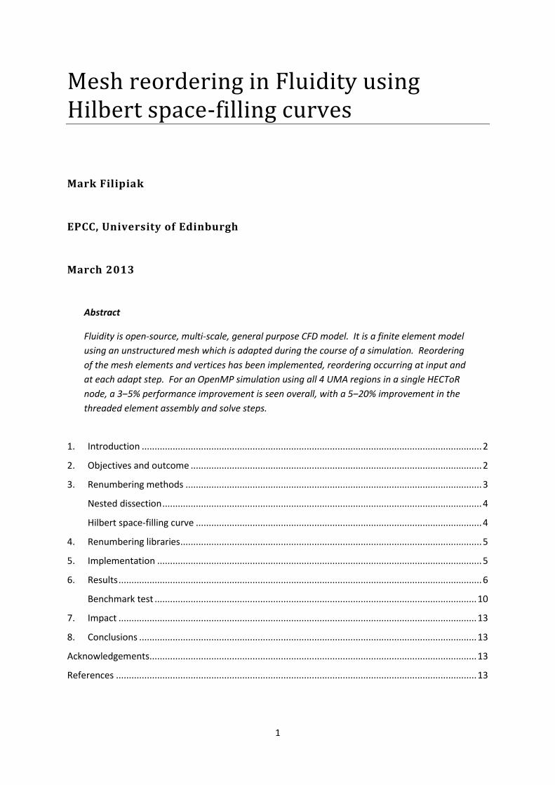
size mesh this will give an ordering of all the nodes. A typical bottom-up method is the Hilbert

space-filling curve method, where a (finite) Hilbert curve (a mapping from [0,1] into the unit square

or cube, see Figure 1) is computed for the physical domain covered by the mesh. The Hilbert

coordinates of the nodes then give an ordering of the nodes [2].

Figure 1: a. 5th

order Hilbert curve in 2D [from en.wikipedia.org, author António Miguel de Campos]. b. 3rd

order Hilbert curve in 3D [from hr.wikipedia.org, author Stevo-88].

a. b. b.

4

The traversal of the hierarchical structure of the dissection or of the curve gives the desired locality

of nodes in the ordering. Nodes that are close in the ordering will be close in the mesh or in the

physical domain. However, there will be ‘boundary’ nodes at all scales which are close in the mesh

or physical domain but which are far apart in the ordering; this cannot be avoided. Both methods

have a hierarchical structure in physical space, so that there is locality at all scales. The locality

property is just what is needed for ensuring physical locality corresponds to memory locality. The

hierarchical property means that the methods can be generally applied without tuning to the actual

number of UMA regions. The hierarchical structure also means that the resulting ordering will also

have good cache locality, no matter what size or number of levels of cache.

The two methods have their advantages and disadvantages:

Nested dissection

Advantages

Mesh-based, so will work with any topology, e.g. thin spherical shells (oceans).

Disadvantages

Choice of sub-mesh size at which to stop the recursion will depend on the cache size of the

processor but usually be much smaller than the size of a UMA region so will still be ‘NUMA-

oblivious’.

May be slow to calculate the bisections.

Hilbert space-filling curve

Advantages

Assuming the machine precision is large enough to generate a high order approximation to

the Hilbert curve, locality will be achieved at all scales, so the ordering will be cache-

oblivious and NUMA oblivious.

Can be fast to calculate the ordering.

Disadvantages

Ordering is based on the physical coordinates and may give poor results for physical

domains with extreme aspect ratios or that are embedded in a higher dimension space, e.g.

spherical shells (oceans). Recent work on mesh traversal by a self-avoiding walk [3] [4] may

lead to a mesh-based analogue of the space-filling curve but it is not clear that it will have

the desired hierarchical structure.

5

4. Renumbering libraries Because of the modularity of the task, and its wide application, renumbering methods have been

implemented in many high performance software libraries. In Table 1 we list the libraries

considered.

Table 1: Possible software libraries for renumbering

Library Open source Parallel Comments

Boost graph library

yes yes Several sparse matrix ordering schemes (only in the serial library).

Leda no no No ordering or decomposition algorithms.

Scotch yes yes Recursive dissection ordering. Scotch is included in Zoltan.

Zoltan yes yes Contains Scotch and ParMetis, and Hilbert space-filling curve ordering.

Chaco yes no Partitioning only.

Jostle no evaluation version only Partitioning only.

ParMetis yes yes Recursive dissection ordering. ParMetis is included in Zoltan.

Zoltan is already integrated into the Fluidity code for load balancing and Zoltan provides Hilbert

space-filling curve ordering and recursive dissection ordering (via its 3rd party libraries ParMetis and

Scotch). Thus Zoltan was the obvious choice of library to use. During the project there was time

only to evaluate the Hilbert space-filling curve method. However, the literature indicates that this is

a particularly good choice cache-oblivious choice for unstructured computation [5]. The

implementation of reordering in Fluidity has been structured so that it is easy to add new ordering

methods and recursive dissection can be added as an option in the future.

5. Implementation The main computation in Fluidity consists of the assembly and solution of the momentum (velocity),

pressure, and transport equations. The velocity, pressure and tracer fields are defined on the same

elements as the basic mesh but can have different order (e.g. quadratic elements) and different

continuity. The meshes for these fields are derived from the basic mesh and will have the same

elements and element connectivity but can have different numbers of nodes and node connectivity

and require ordering separately. Colleagues at Imperial College, London are developing a numbering

scheme for such derived meshes but this still requires that the basic mesh has a good ordering to

start with.

In Fluidity, data structures are hierarchical, with a “state” variable holding the current simulation

state. This state variable holds multiple fields, each of which carry information about the

discretisation they are using, which in turn carries information on the topological mesh. In addition,

any decomposition must also work with extruded and periodic meshes. Extruded meshes are

6

commonly used in oceanic simulations, where a 2-D surface mesh is created and then extruded

downwards to a known bathymetry to create either a z-layered or σ-layered mesh. As such, only the

2-D mesh is decomposed, but the full 3-D mesh must still be ordered correctly. Periodic meshes

contain connectivity between elements on one or more of the domain edges, which must be taken

into account when ordering elements.

An initial step was to convert the code to use the Fluidity-based tool flredecomp instead of the

stand-alone tool fldecomp for the initial decomposition of a mesh when running in parallel. Then

the reordering code could be added to Fluidity only. The regression tests were converted to use

flredecomp and some bugs uncovered by this change were corrected.

The positions of the mesh vertices and element centres are re-ordered together so that the element

ordering matches the node ordering. This gives a permutation to be applied to the meshes and

positions (and auxiliary data structures). These reordered meshes are used as normal in Fluidity to

derive all the other meshes on which the fields are defined.

There are three cases where the topological mesh should be renumbered:

when the initial mesh is input, unless some input data (e.g., from a checkpoint) is defined on the initial mesh;

after the mesh is adapted: this is the easiest case and the new mesh can always be re-ordered since all the fields are interpolated from the old meshes to the new meshes.

in the middle of load balancing, after the basic mesh has been load balanced but before the fields have been re-distributed across the processors. In this case, the mapping from ‘universal’ (over all MPI processes) numbers to ‘global’ (local to one MPI process) numbers also has to be permuted.

The mesh in each process is reordered separately, within each process. This is sufficient to improve

the NUMA and cache performance but does mean that the halo regions, shared between processes,

cannot be reordered: Fluidity exploits a fixed order in the haloes to overlap communications and

computation.

The code is now available as a branch of the Fluidity code (https://code.launchpad.net/~fluidity-core/fluidity/hilbert) and is currently being reviewed for merging into the main development trunk. It will be made generally available at the first available release of Fluidity.

6. Results The code was developed on a local machine that is the equivalent of 2 nodes of HECToR Phase 2.

The regression tests were also performed on this machine. Using reordering is sometimes faster and

sometimes slower for these tests. Over the 50 largest tests, assembly using the reordered meshes

took 95-105% of the time for the unordered meshes, depending on the test. The velocity solve using

the reordered meshes takes 90-120% of the time for the unordered meshes, depending on the test.

However, these tests are all much smaller than real-world simulations, and in many cases the input

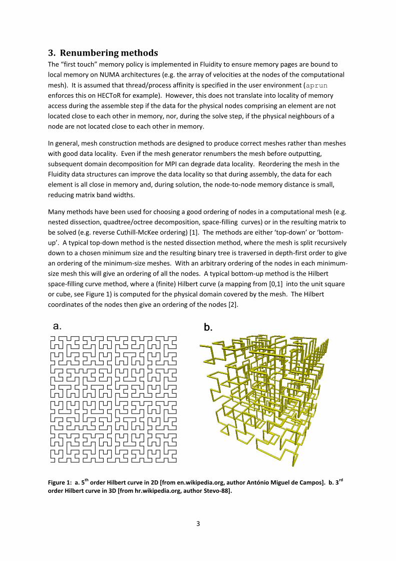
mesh already has a good ordering. Example meshes, original and reordered, are shown in Figure 2,

Figure 3, and Figure 4. The re-ordering of the mesh in each process does not affect the halo regions

shared between processes, as shown in Figure 5.

7

Figure 2: Mesh for 2D tracer diffusion (test case prescribed_adaptivity): a. Original ordering of the coordinate mesh nodes. b. Hilbert ordering of the coordinate mesh nodes.

Figure 3: Mesh for a 3D Stokes flow (test case Stokes_3d_busse_1a_p2p1): a. Original ordering of the coordinate mesh nodes. b. Hilbert ordering of the coordinate mesh nodes.

a.

b.

b.

a.

8

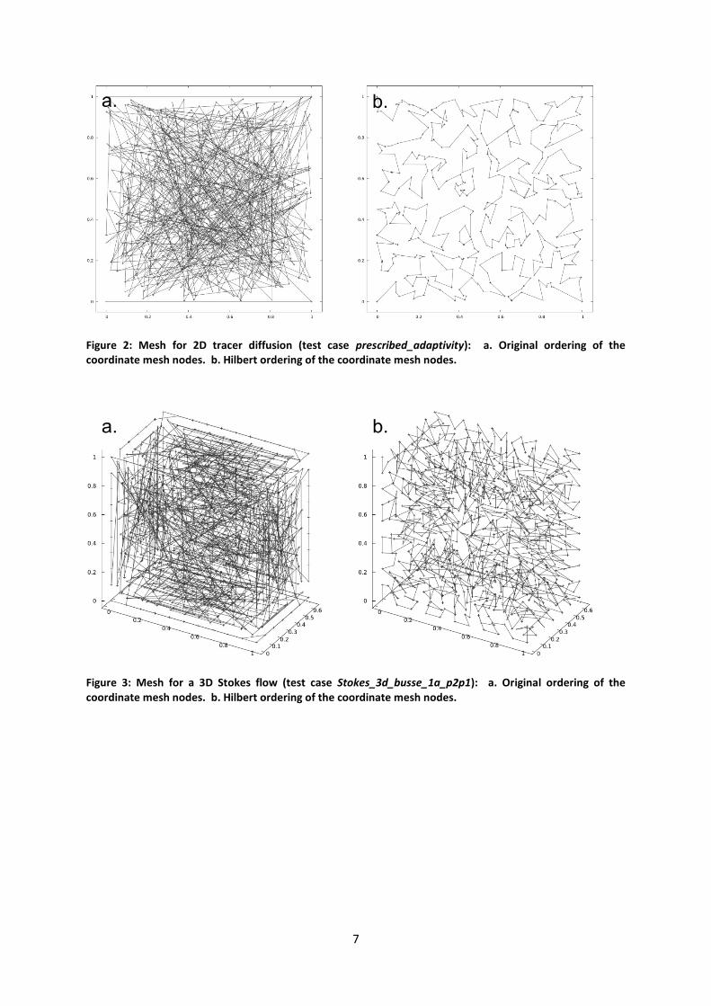
Figure 4:Mesh for a 2D simulation of droplets colliding at an air-water interface (test case 5material-droplet-adapt): a. Mesh after several mesh adaptation steps. b. Ordering just after the last adaptation: the poorly ordered nodes are for elements that have been adapted. c. The reordering after the adaptation restores a good ordering for all nodes.

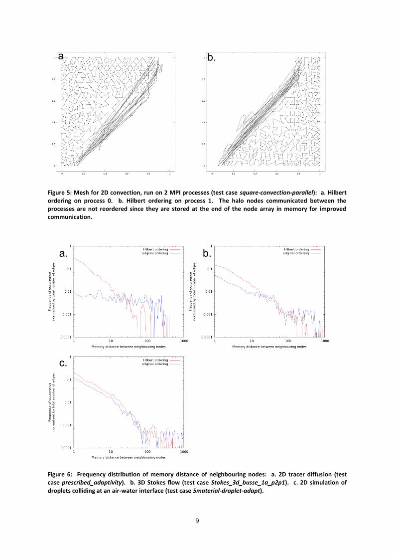
One measure of the improvement in memory locality for the solve step is the distribution of

differences in array index (equivalent to distance in memory) of neighbouring nodes. This

distribution is shown in Figure 6 for the cases used for Figure 2, Figure 3, and Figure 4. The node-

distance distribution shifts to smaller distances when the mesh is re-ordered.

a. b. c.

9

Figure 5: Mesh for 2D convection, run on 2 MPI processes (test case square-convection-parallel): a. Hilbert ordering on process 0. b. Hilbert ordering on process 1. The halo nodes communicated between the processes are not reordered since they are stored at the end of the node array in memory for improved communication.

Figure 6: Frequency distribution of memory distance of neighbouring nodes: a. 2D tracer diffusion (test case prescribed_adaptivity). b. 3D Stokes flow (test case Stokes_3d_busse_1a_p2p1). c. 2D simulation of droplets colliding at an air-water interface (test case 5material-droplet-adapt).

a.

a.

b.

b.

c.

10

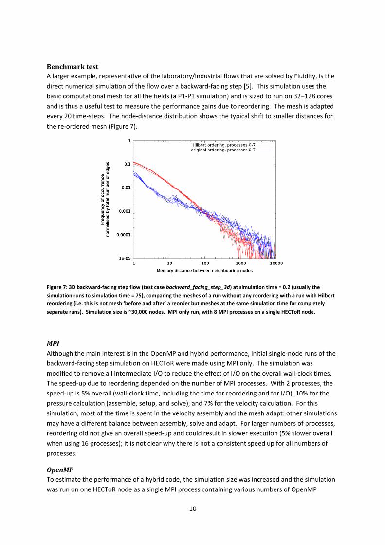
Benchmark test

A larger example, representative of the laboratory/industrial flows that are solved by Fluidity, is the

direct numerical simulation of the flow over a backward-facing step [5]. This simulation uses the

basic computational mesh for all the fields (a P1-P1 simulation) and is sized to run on 32‒128 cores

and is thus a useful test to measure the performance gains due to reordering. The mesh is adapted

every 20 time-steps. The node-distance distribution shows the typical shift to smaller distances for

the re-ordered mesh (Figure 7).

Figure 7: 3D backward-facing step flow (test case backward_facing_step_3d) at simulation time = 0.2 (usually the

simulation runs to simulation time = 75), comparing the meshes of a run without any reordering with a run with Hilbert

reordering (i.e. this is not mesh ‘before and after’ a reorder but meshes at the same simulation time for completely

separate runs). Simulation size is ~30,000 nodes. MPI only run, with 8 MPI processes on a single HECToR node.

MPI

Although the main interest is in the OpenMP and hybrid performance, initial single-node runs of the

backward-facing step simulation on HECToR were made using MPI only. The simulation was

modified to remove all intermediate I/O to reduce the effect of I/O on the overall wall-clock times.

The speed-up due to reordering depended on the number of MPI processes. With 2 processes, the

speed-up is 5% overall (wall-clock time, including the time for reordering and for I/O), 10% for the

pressure calculation (assemble, setup, and solve), and 7% for the velocity calculation. For this

simulation, most of the time is spent in the velocity assembly and the mesh adapt: other simulations

may have a different balance between assembly, solve and adapt. For larger numbers of processes,

reordering did not give an overall speed-up and could result in slower execution (5% slower overall

when using 16 processes); it is not clear why there is not a consistent speed up for all numbers of

processes.

OpenMP

To estimate the performance of a hybrid code, the simulation size was increased and the simulation

was run on one HECToR node as a single MPI process containing various numbers of OpenMP

11

threads. This is analogous to one MPI process of a hybrid code with one MPI process per node. The

difference is that there will be no haloes, which should be a small fraction of the total mesh for large

simulations.

The simulation size was increased from ~30,000 to ~1,000,000 nodes (which takes ~4GB memory: a

HECToR node has 32GB memory) by modifying the adapt parameters and running for a few adapt

steps. The simulation was run again using this larger mesh size and the simulation stopped after 20

time-steps plus the adapt step. This gives enough data, in a reasonable time, to compare the speeds

for unordered and reordered meshes.

The thread placement was chosen to accentuate NUMA effects. A HECToR node has 32 cores

distributed over 4 UMA regions (0, 1, 2, 3). The HyperTransport links between UMA regions 1 and 2

and between regions 0 and 3 have the lowest bandwidth so the threads were arranged as shown in

Table 2.

Table 2: Distribution of threads over UMA regions to accentuate NUMA effects

Number of threads UMA region

0 1 2 3

1 0

2 0 1

4 0 1 2 3

8 0, 1 2, 3 4, 5 6, 7

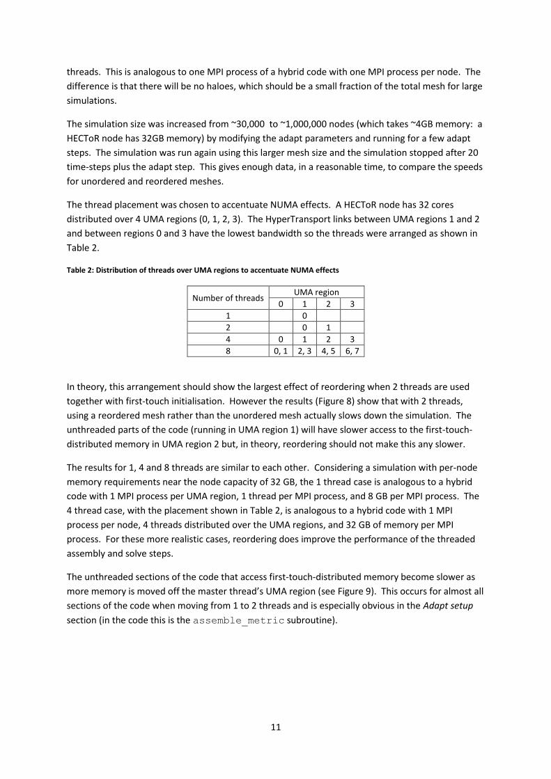
In theory, this arrangement should show the largest effect of reordering when 2 threads are used

together with first-touch initialisation. However the results (Figure 8) show that with 2 threads,

using a reordered mesh rather than the unordered mesh actually slows down the simulation. The

unthreaded parts of the code (running in UMA region 1) will have slower access to the first-touch-

distributed memory in UMA region 2 but, in theory, reordering should not make this any slower.

The results for 1, 4 and 8 threads are similar to each other. Considering a simulation with per-node

memory requirements near the node capacity of 32 GB, the 1 thread case is analogous to a hybrid

code with 1 MPI process per UMA region, 1 thread per MPI process, and 8 GB per MPI process. The

4 thread case, with the placement shown in Table 2, is analogous to a hybrid code with 1 MPI

process per node, 4 threads distributed over the UMA regions, and 32 GB of memory per MPI

process. For these more realistic cases, reordering does improve the performance of the threaded

assembly and solve steps.

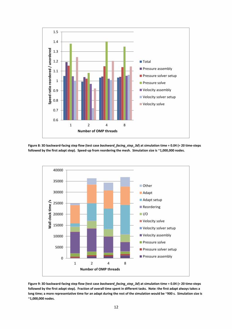
The unthreaded sections of the code that access first-touch-distributed memory become slower as

more memory is moved off the master thread’s UMA region (see Figure 9). This occurs for almost all

sections of the code when moving from 1 to 2 threads and is especially obvious in the Adapt setup

section (in the code this is the assemble_metric subroutine).

12

Figure 8: 3D backward-facing step flow (test case backward_facing_step_3d) at simulation time = 0.04 (= 20 time-steps

followed by the first adapt step). Speed-up from reordering the mesh. Simulation size is ~1,000,000 nodes.

Figure 9: 3D backward-facing step flow (test case backward_facing_step_3d) at simulation time = 0.04 (= 20 time-steps

followed by the first adapt step). Fraction of overall time spent in different tasks. Note: the first adapt always takes a

long time; a more representative time for an adapt during the rest of the simulation would be ~900 s. Simulation size is

~1,000,000 nodes.

0.6

0.7

0.8

0.9

1

1.1

1.2

1.3

1.4

1.5

1 2 4 8

Spe

ed

rat

io r

eo

rde

red

/ u

no

rde

red

Number of OMP threads

Total

Pressure assembly

Pressure solver setup

Pressure solve

Velocity assembly

Velocity solver setup

Velocity solve

0

5000

10000

15000

20000

25000

30000

35000

40000

1 2 4 8

Wal

l clo

ck t

ime

/s

Number of OMP threads

Other

Adapt

Adapt setup

Reordering

I/O

Velocity solve

Velocity solver setup

Velocity assembly

Pressure solve

Pressure solver setup

Pressure assembly

13

7. Impact The usage of the centrally installed Fluidity binary on HECToR has been ~100,000 node hours

(23,000 kAU) per year. Adding reordering to the code will reduce the kAU footprint by 5%, 1000kAU

per year. Hilbert space-filling curve reordering could be applied to other finite element codes

running on HECToR to give a similar improvement.

8. Conclusions Reordering the computational mesh in Fluidity can give speed-ups compared with an unordered

mesh of 5% overall and 5‒20% for assembly and solve but the problem size (per MPI process) has to

be large to achieve this speed-up. Threading with first-touch initialisation in a NUMA system

generally maintains this speed-up.

Acknowledgements This project was funded under the HECToR Distributed Computational Science and Engineering (CSE)

Service operated by NAG Ltd. HECToR – A Research Councils UK High End Computing Service - is the

UK's national supercomputing service, managed by EPSRC on behalf of the participating Research

Councils. Its mission is to support capability science and engineering in UK academia. The HECToR

supercomputers are managed by UoE HPCx Ltd and the CSE Support Service is provided by NAG Ltd.

http://www.hector.ac.uk

References

[1] D. A. Burgess and M. B. Giles, “Renumbering unstructured grids to improve the performance of

codes on hierarchical memory machines,” Advances in Engineering Software, vol. 28, pp. 189-

201, 1997.

[2] S. Aluru and F. Sevilgen, “Parallel domain decomposition and load balancing using space- filling

curves,” in Proc. 4th IEEE International Conference on High Performance Computing, 1997.

[3] G. Heber, R. Biswas and G. R. Gao, “Self-avoiding walks over adaptive unstructured grids,”

Concurrency: Practice and Experience, vol. 12, pp. 85-109, 2000.

[4] H. Liu and L. Zhang, “Existence and construction of Hamiltonian paths and cycles on conforming

tetrahedral meshes,” International Journal of Computer Mathematics, vol. 88, no. 6, pp. 1137-

1143, 2001.

[5] A.-J. N. Yzelman and R. H. Bisseling, “A cache-oblivious sparse matrix--vector multiplication

scheme based on the Hilbert curve,” in Progress in Industrial Mathematics at ECMI 2010, Berlin,

2012.

[6] H. Le, P. Moin and J. Kim, “Direct numerical simulation of turbulent flow over a backward-facing

step,” Journal of Fluid Mechanics, vol. 330, pp. 349-374, 1997.

14