This is the author’s version. The final publication is available at Springer via http://dx.doi.org/10.1007/978-3-319-27174-3

Meta-analytic

structural equation modeling

Suzanne Jak

Department of Methodology and Statistics

Faculty of Social Sciences

Utrecht University

The Netherlands

Department of Psychology

Faculty of Arts and Social Sciences

National University of Singapore

Singapore

Part of this work was supported by Rubicon-grant 446-14-003 from the Nether-

lands Organization for Scientific Research (NWO).

2

Preface Meta-analysis (MA) is a prominent statistical tool in many research disciplines. It

is a statistical method to combine the data of several independent studies, in order

to draw overall conclusions based on the pooled data. Structural equation model-

ing (SEM) is a technique that tests the relations between a set of variables in one

model, for example in a path model or a factor model. In a SEM-analysis, all hy-

pothesized relations between the variables are tested simultaneously. The overall

fit of the model can be evaluated using several fit indices. SEM does not need raw

data, but fits structural equation models to covariance (or correlation) matrices di-

rectly.

The combination of meta-analysis and structural equation modeling for the

purpose of testing hypothesized models is called meta-analytic structural equation

modeling (MASEM). MASEM is a new and promising field of research. With

MASEM, a single model can be tested to explain the relationships between a set

of variables in several studies. By using MASEM, we can profit from all available

information from all available studies, even if few or none of the studies report

about all relationships that feature in the full model of interest.

I use the term MASEM for the process of fitting a structural equation model on

the combined data from several studies. SEM can also be used to perform ordinary

meta-analysis (SEM-based meta-analysis), but this falls outside the scope of this

book.

This book gives an overview of the most prominent methods to perform

MASEM, with a focus on the Two-Stage SEM approach. The fixed and the ran-

dom approach to MASEM are illustrated with two applications to real data. All

steps that have to be taken to perform the analyses are discussed. The data and

syntax files can be found online (http://suzannejak.nl/masem), so that readers can

replicate all analyses.

I would like to thank the editors of the Springer Briefs Series on Research Syn-

thesis and Meta-Analysis, Mike Cheung, Michael Bosnjak, and Wolfgang Viecht-

bauer, for inviting me to write this book and providing me with valuable com-

ments on earlier versions of the manuscript. Of course, all remaining errors are

mine. I also thank Mathilde Verdam for providing feedback on the first chapter,

and Debora Roorda and Huiyong Fan for making their data available.

I am especially grateful to Mike Cheung, who was willing to share his exten-

sive knowledge of MASEM with me during my stay at the National University of

Singapore.

Suzanne Jak, 15 September 2015

3

Contents

Chapter 1 Introduction to meta-analysis and structural equation modeling ... 5 1.1 What is meta-analysis? ................................................................................ 5 1.2 What is SEM? .............................................................................................. 8 1.3 Why should you combine SEM and MA? ................................................. 17 References........................................................................................................ 18

Chapter 2 Methods for meta-analytic structural equation modeling ............ 21 2.1 Introduction ................................................................................................ 21 2.2. Univariate methods ................................................................................... 22 2.3 Multivariate methods ................................................................................. 23 References........................................................................................................ 28

Chapter 3 Heterogeneity ..................................................................................... 31 3.1 Introduction ................................................................................................ 31 3.2 Testing the significance of heterogeneity .................................................. 32 3.3 The size of the heterogeneity ..................................................................... 33 3.4 Random effects analysis or explaining heterogeneity ................................ 34 References........................................................................................................ 36

Chapter 4 Issues in meta-analytic structural equation modeling .................. 38 4.1 Software to conduct MASEM .................................................................... 38 4.2 Fit-indices in TSSEM ................................................................................ 39 4.3 Missing correlations in TSSEM ................................................................. 40 4.4 The ML-approach to MASEM ................................................................... 41 References........................................................................................................ 42

Chapter 5 Fitting a path model with the two-stage approach ......................... 44 5.1 Introduction ................................................................................................ 44 5.2 Preparing the data ...................................................................................... 45 5.3 Fixed effects analysis ................................................................................. 47 5.4 Random effects analysis ............................................................................ 50 5.5 Random effects subgroup analysis ............................................................. 58 References........................................................................................................ 62

Chapter 6 Fitting a factor model with the two-stage approach ...................... 63 6.1 Introduction ................................................................................................ 63 6.2 Preparing the data ...................................................................................... 63 6.3 Fixed effects analysis ................................................................................. 64 6.4 Random effects analysis ............................................................................ 67 References........................................................................................................ 75

Appendix A .......................................................................................................... 77

4

Model implied covariance matrix of the example path model ......................... 77

Appendix B .......................................................................................................... 79 Fitting a path model to a covariance matrix with OpenMx ............................. 79

Appendix C .......................................................................................................... 87 Model implied covariance matrix of the example factor model ...................... 87

Appendix D .......................................................................................................... 88 Fitting a factor model to a covariance matrix with OpenMx ........................... 88

5

Chapter 1 Introduction to meta-analysis and structural equation modeling

Abstract Meta-analysis is a prominent statistical tool in many research disci-

plines. It is a statistical method to combine the effect sizes of separate independent

studies, in order to draw overall conclusions based on the pooled results. Structur-

al equation modeling is a multivariate technique to fit path models, factor models,

and combinations of these to data. By combining meta-analysis and structural

equation modeling, information from multiple studies can be used to test a single

model that explains the relationships between a set of variables or to compare sev-

eral models that are supported by different studies or theories. This chapter pro-

vides a short introduction to meta-analysis and structural equation modeling.

Keywords meta-analysis, introduction, structural equation modeling, path model,

factor model, model fit

1.1 What is meta-analysis?

The term “meta-analysis” was introduced by Glass (1976), who differentiated be-

tween primary analysis, secondary analysis, and meta-analysis. However, the

techniques on which meta-analysis is based were developed much earlier (see

Chalmers et al. 2002; O’Rourke 2007). In the terminology of Glass, primary anal-

ysis involves analyzing the data of a study for the first time. Secondary analysis

involves the analysis of data that have been analyzed before, for example to check

the results of previous analyses or to test new hypotheses. Meta-analysis then in-

volves integration of the findings from several independent studies, by statistically

combining the results of the separate studies. One of the first meta-analyses in the

social sciences was performed by Smith and Glass (1977), who integrated the

findings of 375 studies that investigated whether psychotherapy was beneficial for

patients, a topic that was much debated at the time. By using a quantitative ap-

proach to standardizing and averaging treatment/control differences across all the

studies, it appeared that overall, psychotherapy was effective, and that there is lit-

tle difference in effectiveness across the different types of therapy. Around the

same time as Smith and Glass performed this meta-analysis, other researchers de-

veloped similar techniques to synthesize research findings (Rosenthal & Rubin

1978, 1982; Schmidt & Hunter 1977), which are now all referred to as meta-

analysis techniques. Meta-analysis is used to integrate findings in many fields,

such as psychology, economy, education, medicine, and criminology.

6

1.1.1 Issues in meta-analysis

Compared with primary analysis, meta-analysis has important advantages. Be-

cause more data is used in a meta-analysis, the precision and accuracy of estimates

can be improved. Increased precision and accuracy also leads to greater statistical

power to detect effects.

Despite the obvious positive contributions of meta-analysis, the technique is al-

so criticized. Sharpe (1997) identified the three main validity threats to meta-

analysis: mixing of dissimilar studies, publication bias, and inclusion of poor qual-

ity studies. The mixing of dissimilar studies, also referred to as “mixing apples

and oranges” problem, entails the issue that average effect sizes are not meaning-

ful if they are aggregated over a very diverse range of studies. Card (2012) coun-

ters this critique by stating that it depends on the inference goal whether it is ap-

propriate to include a broad range of studies in the meta-analysis (e.g. if one is

interested in fruit, it is appropriate to include studies about apples, oranges, straw-

berries, banana’s etc.). Moreover, a meta-analysis does not only entail aggregation

across the total pool of studies, but can also be used to compare different subsets

of studies using moderator analysis. The second threat, publication bias, is also re-

ferred to as the “file drawer” problem, and points to the problem that some studies

that have been conducted may not be published, and are therefore not included in

the meta-analysis. Publication bias is a real source of bias, because the non-

published studies are probably those that found non-significant or unexpected re-

sults. Several methods exist that aim at avoiding, detecting and/or correcting for

publication bias (see Rothstein et al. 2006; van Assen et al. 2014) but there is no

consensus on the best ways to deal with the problem. The third issue, the inclusion

of poor quality studies in the meta-analysis is also denoted as the “garbage in, gar-

bage out” problem. Although it may seem logical to leave studies of poor quality

out of the meta-analysis a priori, it is recommended to code the relevant features

of the included primary studies that are required for high quality (e.g. randomiza-

tion in an experiment), so that later on one can investigate whether these quality-

conditions are related to the relevant effect sizes (Valentine 2009).

Cooper and Hedges (2009) distinguish six phases of research synthesis: Prob-

lem formulation, literature search, data evaluation, data analysis, interpretation of

the results and presentation of the results. In this book we focus on the data analy-

sis phase, referred to as meta-analysis. The other parts of research synthesis are

discussed in for example Borenstein et al. (2009), Card (2012), Cooper et al.

(2009), and Lipsey and Wilson (2001).

1.1.2 Statistical analysis

Usually, the units of analysis in a meta-analysis are not the raw data, but summary

statistics (effect size statistics) that are reported in the individual studies. The type

of effect size statistic that is investigated depends on the nature of the variables in-

volved. For example, if the interest is in differences between a treatment and con-

7

trol group on some continuous outcome variable, the meta-analysis may focus on

the standardized mean difference (like Cohen’s d or Hedges’ g). If the hypothesis

is about the association between two continuous variables, the (z-transformed)

product moment correlation coefficient may be the focus of the analysis. If the in-

terest is in association between two dichotomous variables, the (logged) odds ratio

is often an appropriate effect size statistic. Once the effect size statistics of interest

are gathered or reconstructed from the included studies, the statistical analysis can

start, using fixed effects or random effects analysis.

The fixed effects approach is useful for conditional inference, which means that

the conclusions cannot be generalized beyond the studies included in the analysis

(Hedges & Vevea 1998). In the most common fixed effects model, it is assumed

that the effect size statistics gathered from the studies are estimates of one popula-

tion effect size, and differences between studies are solely the result of sampling

error. The analysis focuses on obtaining a weighted mean effect size across stud-

ies. The weights are based on the sampling variance in the studies, so that studies

with larger sampling variance (and smaller sample size) contribute less to the

weighted mean effect size (which is the estimate of the population effect size).

The random effects approach facilitates inferences to studies beyond the ones

included in the particular meta-analysis (unconditional inference). The random ef-

fects approach assumes that the population effect sizes vary from study to study,

and that the studies in the meta-analysis are a random sample of studies that could

have been included in the analysis. Differences in effect sizes between studies are

hypothesized to be due to sampling error and other causes, such as differences in

characteristics of the respondents or operationalization of the variables in the dif-

ferent studies. The random effects analysis leads to an estimate of the mean and

variance of the distribution of effect sizes in the population.

Apart from the average effect size, it is often also of interest if and why studies

differ systematically in their effect size statistics. Therefore, researchers often

code study characteristics (e.g. average age of respondents, measurement instru-

ments used, country in which the study was conducted), and investigate whether

the effect sizes are associated with these study-level variables. This is called mod-

erator analysis, and is used to investigate whether the association between the var-

iables of interest is moderated by study characteristics. These moderator variables

may explain variability in the effect sizes. If all variability is explained, a fixed ef-

fects model may hold, implying that conditional on the moderator variables, all

remaining variability is sampling variability. If effect sizes are regressed on study

level variables in a random effects approach, reflecting that the moderator varia-

bles do not explain all variability across the studies, this is called mixed effects

meta-analysis.

To be consistent with recent terminology, I use the term “fixed effects model”

for all models that do not estimate between-studies variance. This terminology is

common in meta-analysis, but not in line with the statistical literature, where the

fixed effects model denotes the model in which heterogeneity is explained by

study-level variables. The model that assumes homogeneity of effect sizes, with-

8

out study-level variables, is also called the “equal effects model” (Laird & Mostel-

ler, 1990). I use the term “fixed effects model” for both these models, and will ex-

plicitly state when study-level variables are included in the model.

1.2 What is SEM?

Structural equation modeling (SEM) has roots in two very different techniques

developed in two very different fields. Path analysis with its graphical representa-

tions of effects and effect decomposition comes from genetics research, where

Sewall Wright (1920) proposed a method to predict heritability of the piebald pat-

tern of guinea-pigs. Factor analysis is even older, with an early paper by Spearman

in 1904, and was developed in research on intelligence, to explain correlations be-

tween various ability tests (Spearman 1928). Karl Jöreskog (1973) coined the

name LISREL (LInear Structural RELations) for the framework that integrates the

techniques of path analysis and factor analysis, as well as for the computer pro-

gram that made the technique available to researchers.

1.2.1 Path analysis

SEM is a confirmatory technique, which means that a model is formulated based

on theory, and it is judged whether this model should be rejected by fitting the

model to data. If multivariate normality of the data holds, the variance covariance

matrix of the variables of interest and the sample size are sufficient to fit models

to the data. This is a very convenient aspect of SEM, because it means that as long

as authors report correlations and standard deviations of their research variables in

their articles, other researchers are able to replicate the analyses, and to test differ-

ent hypotheses on these data. In order to test hypotheses, these hypotheses have to

be translated in a statistical model. The statistical model can be formulated in dif-

ferent ways, for example using a graphical display. The graphical displays that are

used for structural equation models use squares to represent observed variables, el-

lipses to represent latent variables, one-headed arrows to represent regression co-

efficients, and two-headed arrows to represent covariances. Consider the path

model in Figure 1.1, in which the effect of negative and positive relations with

teachers is hypothesized to affect student achievement through student engage-

ment.

9

Figure 1.1 Hypothesized path model in which the effects of Positive and Negative

relations on Achievement is fully mediated by Engagement

The four observed variables are depicted in squares. Student engagement is re-

gressed on Positive and Negative relations, and Student Achievement is regressed

on Student Engagement. There are no direct effects of Positive and Negative rela-

tions on Student Achievement, reflecting the hypothesis that these effects are fully

mediated by Student Engagement. In this model, Engagement and Achievement

are called endogenous variables, reflecting that other variables are hypothesized to

have an effect on them. Variables that are not regressed on other variables are

called exogenous variables. Positive and Negative relations are exogenous varia-

bles in this model. The two exogenous variables are assumed to covary, indicated

by the two-headed arrow between them. There are also two-headed arrows point-

ing from the variable to itself, reflecting the variance of the variable (a covariance

with itself is equal to a variance). The endogenous variables have a latent variable

with variance pointing to it. This latent variable is called a residual factor, and

could be viewed as a container variable representing all other variables that also

explain variance in the endogenous variable, but that are not included in the mod-

el. The regression coefficient of the variable on the residual factor is not estimated

but fixed at 1 for identification of the model. The variance of the residual factor

represents the unexplained variance of the endogenous variable. So, part of the

variance in Student Engagement is explained by Positive and Negative relations,

and the remaining variance is residual variance (or, unexplained variance). Simi-

larly, part of the variance in Student Achievement is explained by Student En-

gagement, and the remaining variance is residual variance. For the exogenous var-

iables, actually, all variance is unexplained. So it seems logical to depict two more

residual factors with variance pointing to Negative and Positive relations, instead

of the double headed arrow pointing to the variables themselves. Indeed, this

would be correct, but to keep the graphs simple they are often not depicted. Actu-

1. Positive teacher-student relations

2. Negative teacher-student

relations

3. Student engagement

4. Student achievement

ψ21

β31

β32

β43

ψ33 ψ44

ψ11

ψ22

ε3

1

ε4

1

10

ally, the residual factor pointing to an endogenous variables is also often not fully

depicted, but represented by a small one-sided arrow.

Attached to the arrows in the graphical display, the Greek symbols represent

the model parameters. In a path model, the direct effects are often denoted by β

and variances and covariances by ψ. For example, β43 represents the regression

coefficient of Variable 4 on Variable 3, ψ44 represents the residual variance of

Variable 4, and ψ21 represents the covariance between Variable 1 and Variable 2.

The model parameters are collected in matrices. A path model on observed varia-

bles can be formulated using two matrices with parameters, matrix Β and matrix

Ψ, and an identity matrix, I. For the example, these matrices look as follows, with

rows 1 to 4 and columns 1 to 4 corresponding to the variables Positive relations,

Negative relations, Student Achievement, and Student Engagement, respectively:

Β =[

0 00 0

0 0 0 0

β31 β32

0 0

0 0 β43 0

], Ψ = [

ψ11 ψ21 ψ22

0 0

0 0

ψ33 0 ψ44

] and I = [

1 00 1

0 00 0

0 00 0

1 00 1

].

Matrix Ψ is a symmetrical matrix, so the covariance between Variables 1 and 2 is

equal to the covariance between Variable 2 and 1. Using these parameters, a mod-

el implied covariance matrix (Σmodel) can be formulated. The model implied covar-

iance matrix is a function of the matrices with parameters:

Σmodel = (I - Β)-1 Ψ (I - Β)-1T . (1.1)

The resulting model implied covariance matrix (Σmodel) for the current example

can be found in Appendix A. The basic hypothesis that is tested by fitting a struc-

tural equation model to data is:

Σ = Σmodel . (1.2)

Note however, that the population covariance matrix, Σ, is generally unavailable

to the researcher, who only observed a covariance matrix based on a sample, de-

noted S. Suppose that observed covariance matrix of the four variables based on

104 respondents is as given in Table 1.1.

11

Table 1.1 Variances (on diagonal) and covariances of four research variables, N =

104

Variable 1. 2. 3. 4.

1. Positive relations

0.81

2. Negative relations -0.36 1.21

3. Engagement 0.63 -0.60 1.69

4. Achievement 0.14 -0.33 0.50 1.44

The model parameters that make up Σmodel can be estimated by minimizing a

discrepancy function. This means that parameters are estimated in order to mini-

mize the difference between the model implied covariance matrix (Σmodel), and the

observed covariance matrix (S). The more parameters a model has, the easier it is

to make the Σmodel close to S. The maximum number of parameters that a model

can have in order to be identified is equal to the number of observed variances and

covariances in S. In our example with four variables, the number of variances and

covariances is ten. The number of parameters in the Σmodel equals eight (three re-

gression coefficients, one covariance, four variances). The degrees of freedom (df)

of a model are equal to the difference between these two. This model has 2 de-

grees of freedom. The larger the degrees of freedom of a model is, the more the

model is a simplification of reality. Simple models are generally preferred over

complicated models. But, the larger the degrees of freedom, the larger the differ-

ence between Σmodel and S will be, meaning that the absolute fit of a model will be

worse.

Having less parameters than observed variances and covariances is not the only

requirement for identification of the model. For a model to be identified, all pa-

rameters in the model need to be identified. See Bollen (1989) for an overview of

methods to assess the identification of model parameters. If a model is identified,

the parameters can be estimated. The most used estimation method is maximum

likelihood (ML) estimation. The discrepancy function FML that is minimized with

ML estimation is:

FML = log| Σmodel | – log|S| + trace(S Σmodel-1) – p, (1.3)

where p is the number of variables in the model. If the model fits the data perfect-

ly, the model implied covariance matrix will be equal to S, and FML will be zero. If

the model does not fit perfectly, FML will be larger than zero. See Bollen (1989)

for a description of ML and other estimation methods and their assumptions.

1.2.2 Model fit

An important property of the ML estimator is that it provides a test of overall

model fit for models with positive degrees of freedom. Under the null hypothesis

12

(Σ = Σmodel), the minimum FML multiplied by the sample size minus one (n-1) as-

ymptotically follows a chi-square distribution, with degrees of freedom equal to

the number of non-redundant elements in S minus the number of model parame-

ters. If the chi-square value of a model is considered significant, the null hypothe-

sis is rejected. The chi-square of a model may become significant because the dis-

crepancy between S and the estimated Σmodel is large, or because the sample is

large. With a very large sample, small differences between S and the estimated

Σmodel may lead to a significant chi-square, and thus rejection of the model. Other

fit measures are available in SEM, which do not test exact fit of the model, but are

based on the idea that models are simplifications of reality and will never exactly

hold in the population. The Root Mean Squared Error of Approximation

(RMSEA, Steiger & Lind 1980) is the most prominent fit measure next to the chi-

square. The RMSEA is interpreted using suggested cut-off values that should be

regarded as rules of thumb. RMSEA values smaller than 0.05 are considered to

indicate close fit, values smaller than 0.08 are considered satisfactory and values

over .10 are considered indicative of bad fit (Browne & Cudeck 1993). Another

prominent fit measure is the Comparitive Fit Index (CFI, Bentler 1990) that is

based on a comparison of the hypothesized model with the “independence model”,

which is a model in which all variables are unrelated. CFI values over .95 indicate

reasonably good fit. For an overview of these and other fit indices see Schermel-

leh-Engel et al. (2003).

Fitting the model from Figure 1 to the observed covariance matrix in Table 1.1

gives the following fit indices: χ2 = 2.54, df = 2, p = .28, RMSEA = .05 and CFI =

.99. So, exact fit of the model is not rejected, and the model also fitted the data ac-

cording to the rules of thumb for the RMSEA and CFI. If the model fits the data,

the parameter estimates can be interpreted. If a model does not fit the data, the pa-

rameter estimates should not be interpreted because they will be wrong. Table 1.2

gives an overview of the unstandardized parameter estimates, the 95% confidence

intervals and the standardized parameter estimates of the model. See Appendix B

for an example of an OpenMx-script to fit the current model.

13

Table 1.2 Unstandardized parameter estimates, 95% confidence intervals and

standardized parameter estimates of the path model from Figure 1.1

Parameter Unstandardized

estimate

95% confidence

interval

Standardized

estimate

lower

bound

upper

bound

β31 0.64 0.40 0.89 0.45

β32 -0.30 -0.50 -0.10 -0.26

β43 0.30 0.13 0.47 0.32

ψ21 -0.36 -0.60 -0.36 -0.36

ψ11 0.81 0.62 1.08 1.00

ψ22 1.21 0.93 1.61 1.00

ψ33 1.10 0.85 1.47 0.65

ψ44 1.29 0.99 1.72 0.90

β31 x β43 0.19 0.08 0.34 0.14

β32 x β43 -0.09 -0.19 -0.03 -0.08

All parameters in this model differ significantly from zero, as judged by the

95% confidence intervals. For interpretation, it is useful to look at the standardized

parameter estimates. For example, the standardized β31, means that 1 standard de-

viation increase in Positive relationships is associated with 0.45 standard devia-

tions increase in Engagement, controlled for the effect of Negative relationships.

The standardized residual variance is interpreted as the proportion of residual var-

iance. This means that in the standardized solution, the proportion of explained

variance in Student achievement is calculated as 1- ψ44, = 0.10. The proportion of

explained variance in Engagement is 0.35. Indirect effects are calculated as the

product of the two direct effects that constitute the indirect effect. With OpenMx,

one can estimate confidence intervals for indirect effects as well. The indirect ef-

fects of Positive and Negative relationships on Student Achievement are both

small but significant (see the last two rows in Table 1.2). This shows that as ex-

pected, there is significant mediation. Whether there is full or partial mediation

can be investigated by testing the significance of the direct effects of Positive and

Negative relationships on Student Achievement. This is shown in Chapter 5.

1.2.3 Factor analysis

Factor analysis can also be seen as a special case of structural equation modeling.

Factor models involve latent variables that explain the covariances between the

observed variables. Consider the two-factor model on five scales measuring chil-

dren’s problem behavior depicted in Figure 1.2.

14

Figure 1.2 A two-factor model on the five problem behavior variables.

In a factor model, each indicator is affected by a common factor that explains

the covariances between the indicators. The regression coefficients linking the fac-

tor to an indicator are called factor loadings. The larger a factor loading is, the

more variance the factor explains in the indicator. Not all indicator variance may

be common variance, which is reflected by the residual factors that affect each in-

dicator. The variance of these residual factors is called residual variance (denoted

by θ) and is assumed to consist of random error variance and structural variance.

For example, there may be a structural component in Somatisation that is not cor-

related with Anxiety or Withdrawn behavior.

With factor analysis, Σmodel is a function of factor loadings, depicted by λ’s,

factor variances and covariances, depicted by φ’s, and residual variances, depicted

by θ’s. Note that one factor loading for each factor is fixed at 1. This is needed to

identify the model. As factors are unobserved variables, the scale of the variables

is not known, and a metric has to be given to the factors by fixing one factor load-

ing per factor. Alternatively, one can fix the factor variances φ11 and φ22 at some

value (e.g. 1) and estimate all factor loadings. In advanced models (e.g. mul-

tigroup and longitudinal models) one method of scaling may be preferred over the

other, but in this example it is arbitrary how the factors are given a metric. The un-

standardized parameters will differ based on the scaling method, but the model fit

and the standardized parameter estimates will not. The factor model can be repre-

sented by three matrices with parameters, a full matrix Λ with factor loadings, a

symmetrical matrix Φ with factor variances and covariances, and a symmetrical

1. Withdrawn 2. Somatisation 3. Anxiety 4. Delinquency 5. Aggression

Internalizing Externalizing

ε1 ε2 ε3 ε4 ε5

11

1 1 1 1 1

φ11 φ22

φ21

λ21λ31

λ52

θ11 θ22θ33 θ44 θ55

15

matrix Θ with residual variances and covariances. For the current model, the three

matrices look as follows.

Λ =

[

1 0λ21 0λ31 00 10 λ52]

, Φ = [φ11 φ21 φ22

] and Θ = ||

θ11 0 θ22 0 0 θ33 0 0 0 θ44 0 0 0 0 θ55

||.

The rows of Λ are associated with variables 1 through 5 from Figure 1.2, as well

as the rows and columns of Θ. The columns of Λ and the rows and columns of Φ

are associated with the Internalizing and Externalizing factors respectively.

The factor model is specified using these matrices as:

Σmodel = Λ Φ ΛT + Θ, (1.4)

leading to the model implied covariance matrix given in Appendix C.

Suppose that we observed the covariance matrix of the five variables from a

sample of 155 parents with children suffering from epilepsy that is given in Table

1.3.

Table 1.3 Variances (on diagonal) and covariances of five research variables

Variable 1. 2. 3. 4. 5.

1. Withdrawn 12.55

2. Somatization 6.31 10.06

3. Anxiety 11.15 9.64 26.02

4. Delinquency 2.85 2.09 4.84 3.72

5. Aggression 12.44 9.68 22.20 9.96 51.02

Fitting the model from Figure 1.2 to these data leads to good fit with the fol-

lowing fit measures: χ2 = 4.08, df = 4, p = .40, RMSEA = .01 and CFI = 1.00. The

unstandardized parameter estimates, 95% confidence intervals and standardized

parameter estimates are given in Table 1.4. All standardized factor loadings are

larger than .70, meaning that they are substantially indicative of the common fac-

tor on which they load. The correlation between the common factors internalizing

and externalizing is significant and quite large, 0.72. The proportion of explained

variance is largest in indicator 5 (1 – 0.11 = 0.89) and smallest in indicator 2 (1 –

0.51 = 0.49). See Appendix D for an annotated OpenMx-script from this example.

16

Table 1.4 Unstandardized parameter estimates, 95% confidence intervals and

standardized parameter estimates of the factor model from Figure 1.2

Parameter Unstandarized

estimate

95% confidence

interval

Standardized

estimate

lower

bound

upper

bound

λ11 1 - - 0.74

λ21 0.85 0.11 8.03 0.70

λ31 1.78 0.18 9.25 0.86

λ42 1 - - 0.77

λ52 4.54 0.50 9.04 0.94

φ11 6.78 1.37 4.96 1

φ22 2.18 0.43 5.11 1

φ21 2.78 0.54 5.16 0.72

θ11 5.69 0.84 6.81 0.46

θ22 5.12 0.707 7.252 0.51

θ33 6.78 1.571 4.314 0.26

θ44 1.52 0.255 5.936 0.41

θ55 5.72 3.945 1.451 0.11

In the two examples given in this chapter the input matrix was a covariance

matrix. Maximum likelihood estimation assumes analysis of the covariance ma-

trix, and not of the correlation matrix. However, sometimes only the correlation

matrix is available. Treating the correlation matrix as a covariance matrix leads to

incorrect results when estimating confidence intervals or when testing specific hy-

potheses (Cudeck 1989). To obtain correct results, a so-called estimation con-

straint can be added. This constraint enforces the diagonal of the model implied

correlation matrix to always consist of 1’s during the estimation.

The factor model and path model are the two basic models within the structural

equation modeling framework. Once a factor model has been established, the

analysis often goes some steps further, for example by including predictor varia-

bles like age to investigate age differences in the latent variables Internalizing and

Externalizing problems. Another extension is multigroup modeling, in which a

model is fitted to covariance matrices from different groups of respondents simul-

taneously, giving the opportunity to test the equality of parameters across groups.

For example, in the path model from Figure 1, it may be hypothesized that the ef-

fect of Positive and Negative relations on Engagement may be stronger for chil-

dren in elementary school than for children in secondary school.

Some cautions about SEM have to be considered. If a model fits the data well,

and is accepted by the researcher as the final model, it does not mean that the

model is the correct model in the population. If the model is not rejected, this

could be due to lack of statistical power to reject the model. Moreover, there may

be other models that fit the data just as well as the hypothesized model. Therefore,

it is important to consider equivalent models (MacCallum et al. 1993). If a model

17

is rejected however, the conclusion is that the model does not hold in the popula-

tion. This chapter is far too short to discuss all relevant issues in SEM. Several

books have been written that can be used to learn about SEM, see for example

Bollen (1989), Byrne (e.g. 1998), Geiser (2012), Loehlin (2004), and Kline

(2011).

1.3 Why should you combine SEM and MA?

Most research questions are about relations (or differences) between a set of vari-

ables. The hypothetical model in Figure 1.1 for example, states that positive and

negative relations lead to achievement through engagement. Current practice in

meta-analysis is to meta-analyze each effect in this model separately. The ques-

tions these analyses answer are: What is the pooled effect of positive relations on

engagement? And: What is the pooled effect of engagement on achievement?

However, what the researcher also may want to know is: Is this model a good rep-

resentation of the data? Are the effects of positive and negative relations on

achievement fully mediated by engagement? Which effects are lacking in this

model?

Using MASEM, information from multiple studies is used to test a single mod-

el that explains the relationships between a set of variables or to compare several

models that are supported by different studies or theories (Becker 1992;

Viswesvaran & Ones 1995). MASEM provides the researcher measures of overall

fit of a model, as well as parameter estimates with confidence intervals and stand-

ard errors. By combining meta-analysis and SEM, some of the difficulties in the

separate fields may be overcome.

Structural equation modelling requires large sample sizes. Small samples lead

to low statistical power, and non-rejection of models. If several (small) studies in-

vestigate the same phenomenon, they may end up with very different final models,

leading to a wide array of models describing the same phenomena. By combining

the information from several (possibly underpowered) primary studies, general

conclusions can be reached about which model is most appropriate. Norton et al.

(2013) for example, used MASEM to investigate the factor structure of an anxiety

and depression scale, by comparing ten different models that were proposed based

on different primary studies. Furthermore, MASEM can be used to answer re-

search questions that are not addressed in any of the primary studies. Even about

models that include a set of variables that none of the primary studies included all

in their study. For example, Study 1 may report correlations between variable A

and variable B. Study 2 may report correlations between variables B and C, and

Study 3 between variable A and C. Although none of the studies included all vari-

ables, one model can be fit on these three variables using MASEM (Viswesvaran

& Ones 1995).

I use the term MASEM for the process of fitting a structural equation model on

the combined data from several studies. SEM can also be used to perform ordinary

18

meta-analysis (SEM-based meta-analysis). SEM-based meta-analysis is outside

the scope of this book, but see Cheung (2008, 2015) for an explanation.

MASEM is a fairly young field of research, and it seems to be growing in pop-

ularity, both in substantive and methodological research. At this moment, a special

issue about MASEM is being edited for the journal Synthesis Research Methods.

References

Becker, B.J. (1992). Using results from replicated studies to estimate linear mod-

els. Journal of Educational Statistics, 17, 341-362.

Bentler, P.M. (1990). Comparative fit indexes in structural models. Psychological

Bulletin, 107, 238-246.

Bollen, K.A.(1989). Structural equations with latent variables. New York, NY:

Wiley.

Borenstein, M., Hedges, L.V., Higgins, J.P.T., & Rothstein, H. (2009). Introduc-

tion to meta-analysis. Hoboken, NJ: Wiley.

Browne, M.W., & Cudeck, R. (1992). Alternative ways of assessing model fit. So-

ciological Methods & Research, 21, 230-258.

Byrne, B.M. (1998). Structural Equation Modeling with LISREL, PRELIS, and

SIMPLIS: Basic Concepts, Applications, and Programming. Mahwah,

NJ: Lawrence Erlbaum Associates Inc.

Card, N.A. (2012). Applied Meta-analysis for Social Science Research. New

York, NY: Guilford Press.

Chalmers, I., Hedges, L.V. and Cooper, H. (2002). A brief history of research syn-

thesis. Evaluation & the Health Professions 25(1), 12–37.

Cheung, M.W.-L. (2008). A model for integrating fixed-, random-, and mixed-

effects meta-analyses into structural equation modeling. Psychological

methods, 13(3), 182-202.

Cheung, M.W.-L. (2015). Meta-Analysis: A Structural Equation Modeling Ap-

proach. Chichester, UK: Wiley.

Cooper, H., Hedges, L.V. & Valentine, J.C. (Eds.). (2009). The handbook of re-

search synthesis and meta-analysis. New York, NY: Russell Sage.

Cooper, H.M., & Hedges, L.V. (2009). Research synthesis as a scientific enter-

prise. In H. Cooper, L.V. Hedges, & J.C. Valentine (Eds.), The handbook

of research synthesis and meta-analysis (pp. 3-16). New York, NY: Rus-

sell Sage.

Cudeck, R. (1989). Analysis of correlation matrices using covariance structure

models. Psychological Bulletin, 105(2), 317-327.

Geiser, C. (2012). Data analysis with Mplus. New York, NY: Guilford.

Glass, G.V. (1976). Primary, secondary, and meta-analysis of research. The Edu-

cational Researcher, 10, 3-8.

Hedges, L.V., & Vevea, J.L. (1998). Fixed-and random-effects models in meta-

analysis. Psychological methods, 3, 486.

19

Jöreskog, K.G. (1973). Analysis of covariance structures. Multivariate analysis, 3,

263-85.

Kline, R.B. (2011). Principles and practice of structural equation modeling. New

York, NY: Guilford.

Laird, N.M., & Mosteller, F. (1990). Some statistical methods for combining ex-

perimental results. International journal of technology assessment in

health care, 6, 5-30.

Lipsey, M.W. & Wilson, D.B. (2001). Practical meta-analysis. Thousand Oaks,

CA: Sage Publications.

Loehlin, J.C. (1998). Latent variable models: An introduction to factor, path, and

structural analysis. Mahwah, NJ: Lawrence Erlbaum Associates Publish-

ers.

MacCallum, R. C., Wegener, D.T., Uchino, B.N., & Fabrigar, L.R. (1993). The

problem of equivalent models in applications of covariance structure

analysis. Psychological bulletin, 114(1), 185-199.

Norton, S., Cosco, T., Doyle, F., Done, J., & Sacker, A. (2013). The Hospital

Anxiety and Depression Scale: A meta confirmatory factor analysis.

Journal of Psychosomatic Research, 74, 74-81.

O’Rourke, K. (2007). An historical perspective on meta-analysis: dealing quantita-

tively with varying study results. Journal of the Royal Society of Medi-

cine, 100(12), 579-582.

Rothstein, H. R., Sutton, A.J., & Borenstein, M. (Eds.). (2005). Publication bias in

meta-analysis Prevention, assessment and adjustments. Hoboken, NJ:

Wiley.

Rosenthal, R., & Rubin, D.B. (1978). Interpersonal expectancy effects: The first

345 studies. Behavioral and Brain Sciences, 1(03), 377-386.

Schermelleh-Engel, K., Moosbrugger, H., & Müller, H. (2003). Evaluating the fit

of structural equation models: Tests of significance and descriptive

goodness-of-fit measures. Methods of psychological research online,

8(2), 23-74.

Schmidt, F.L., & Hunter, J.E. (1977). Development of a general solution to the

problem of validity generalization. Journal of Applied Psychology, 62(5),

529-540.

Sharpe, D. (1997). Of apples and oranges, file drawers and garbage: Why validity

issues in meta-analysis will not go away. Clinical psychology review,

17(8), 881-901.

Smith, M.L. & Glass, G.V. 1977. Meta-analysis of psychotherapy outcome stud-

ies. American Psychologist, 32, 752–760.

Spearman, C. (1904). " General Intelligence," Objectively Determined and Meas-

ured. The American Journal of Psychology, 15(2), 201-292.

Spearman, C. (1928). The sub-structure of the mind. British Journal of Psycholo-

gy. General Section, 18(3), 249-261.

20

Steiger, J.H., & Lind, J.C. (1980, May). Statistically based tests for the number of

common factors. Paper presented at the annual meeting of the Psycho-

metric Society, Iowa City, IA (Vol. 758).

Valentine, J. C. (2009). Judging the quality of primary research. In H. Cooper, L.

V. Hedges, & J.C. Valentine (Eds.), The handbook of research synthesis

and meta-analysis (pp. 129-146). New York, NY: Russell Sage.

van Assen, M.A.L.M., van Aert, R.C.M., & Wicherts, J.M. (2014, November 17).

Meta-analysis using effect size distributions of only statistically signifi-

cant studies. Psychological methods. Advance online publication.

http://dx.doi.org/10.1037/met0000025

Viswesvaran, C., & Ones, D. (1995). Theory testing: Combining psychometric

meta-analysis and structural equations modeling. Personnel Psychology,

48, 865-885.

Wright, S. (1920). The relative importance of heredity and environment in deter-

mining the piebald pattern of guinea–pigs. Proceedings of the National

Academy of Sciences, 6, 320–332.

21

Chapter 2 Methods for meta-analytic structural equation modeling

Abstract The process of performing meta-analytic structural equation modeling

(MASEM) consists of two stages. First, correlation coefficients that have been

gathered from studies have to be combined to obtain a pooled correlation matrix

of the variables of interest. Next, a structural equation model can be fitted on this

pooled matrix. Several methods are proposed to pool correlation coefficients. In

this chapter, the univariate approach, the generalized least squares (GLS) ap-

proach, and the Two Stage SEM approach are introduced. The univariate ap-

proaches do not take into account that the correlation coefficients may be correlat-

ed within studies. The GLS approach has the limitation that the Stage 2 model has

to be a regression model. Of the available approaches, the Two Stage SEM ap-

proach is favoured for its flexibility and good statistical performance in compari-

son with the other approaches.

Keywords meta-analytic structural equation modeling, univariate meta-analysis,

multivariate meta-analysis, GLS-approach, two-stage structural equation model-

ing, MASEM

2.1 Introduction

As shown in Chapter 1, a structural equation model can be fitted to the covariance

or correlation matrix of the variables of interest, without requirement of the raw

data. Therefore, if articles report the correlations between the research variables

(or information that can be used to estimate the correlation), the results can be

used in a meta-analysis. MASEM combines structural equation modeling with me-

ta-analysis by fitting a structural equation model on a meta-analyzed covariance or

correlation matrix. As the primary studies in a meta-analysis often involve varia-

bles that are measured in different scales, MASEM is commonly conducted using

a pooled correlation rather than covariance matrix. In the remainder of this book I

will therefore focus on correlation matrices (but see Beretvas & Furlow 2006;

Cheung & Chan 2009). MASEM typically consists of two stages (Viswesvaran &

Ones 1995). In the first stage, correlation coefficients are tested for homogeneity

across studies and combined together to form a pooled correlation matrix. In the

second stage, a structural equation model is fitted to the pooled correlation matrix.

In the next sections I outline the different approaches to pool correlation coeffi-

cients under the assumption that the correlations are homogenous across studies

(fixed effects approaches). Heterogeneity of correlation coefficients and random

effects approaches are discussed in Chapter 3.

22

2.2. Univariate methods

In the univariate approaches, the correlation coefficients are pooled separately

across studies based on bivariate information only. Dependency of correlation co-

efficients within studies is not taken into account (as opposed to multivariate

methods, described in the next section). In the univariate approaches, a population

value is estimated for each correlation coefficient separately. For one correlation

coefficient, for each study i, the correlation coefficient is weighted by the inverse

of the estimated sampling variance (the squared standard error), vi. The sampling

variance of the correlation between variables A and B is given by:

vi_AB = (1 – ρi_AB2)2 / ni , (2.1)

where ni is the sample size in study i, and the observed correlation ri_AB can be

plugged in for the unknown population correlation ρi_AB. By taking the average of

the weighted correlation coefficients across the k studies, one obtains the synthe-

sized population correlation estimate:

�̂� = ∑

1

𝑣𝑖_𝐴𝐵 𝑟𝑖_𝐴𝐵

𝑘𝑖=1

∑ 1

𝑣𝑖_𝐴𝐵 𝑘

𝑖=1

. (2.2)

Weighting by the inverse sampling variance ensures that more weight is given to

studies with larger sample size (and thus smaller sampling variance). Because the

sampling variance of a correlation coefficient depends on the absolute value of the

correlation coefficient, some researchers (e.g. Hedges & Olkin 1985) proposed to

use Fisher’s z-transformation on the correlation coefficients before synthesizing

the values. The estimated sampling variance vi of a transformed correlation z in a

study i is equal to 1 / (ni - 3), where ni is the sample size in study i. After obtaining

the pooled z-value, it can be back-transformed to an r-value for interpretation.

There is no consensus on whether it is better to use the untransformed correla-

tion coefficient r or the transformed coefficient z in meta-analysis (see Corey et al.

1998). Hunter and Schmidt (1990) argued that averaging r leads to better esti-

mates of the population coefficient than averaging z. However, several simulation

studies (Cheung & Chan 2005; Furlow & Beretvas 2005; Hafdahl & Williams

2009) showed that differences between the two methods were generally very

small, but when differences are present, the z approach tends to do better. If a ran-

dom effects model is assumed however, Schulze (2004) recommends r over z.

If the correlation coefficients are pooled across studies (using the r or z meth-

od), one pooled correlation matrix can be constructed from the separate coeffi-

cients. The hypothesized structural model is then fit to this matrix, as if it was an

observed matrix in a sample.

23

Apart from the problem that the correlations are treated as independent from

each other within a study, the univariate methods have more issues (Cheung &

Chan 2005). Because not all studies may include all variables, some Stage 1 corre-

lation coefficients will be based on more studies than others. This leads to several

problems. First, it may lead to non-positive definite correlation matrices (Wothke

1993), as different elements of the matrix are based on different samples. Non-

positive definite matrices cannot be analysed with structural equation modeling.

Second, correlation coefficients that are based on less studies are estimated with

less precision and should get less weight in the analysis, which is ignored in the

standard approaches. Third, if different sample sizes are associated with different

correlation coefficients, it is not clear which sample size has to be used in Stage 2.

One could for example use the mean sample size, the median sample size or the

total sample size, leading to different results regarding fit indices and statistical

tests in Stage 2. Due to these difficulties, univariate methods are not recommended

for MASEM (Becker 2000; Cheung & Chan 2005).

2.3 Multivariate methods

The two best known multivariate methods for meta-analysis are the generalized

least squares (GLS) method (Becker 1992, 1995, 2009) and the Two-Stage SEM

method (Cheung & Chan 2005). Both will be explained in the next sections.

2.3.1 The GLS method

Becker (1992, 1995, 2009) proposed using generalized least squares estimation to

pool correlation matrices, taking the dependencies between correlations into ac-

count. This means that not only the sampling variances in each study are used to

weight the correlation coefficients, but also the sampling covariances. The esti-

mate of the population variance of a correlation coefficient was given in Equation

2.1. The population covariance between two correlation coefficients, let’s say be-

tween variables A and B and between the variables C and D, is given by the long

expression:

cov(ρi_AB, ρi_CD) =

(0.5ρi_ABρi_BC (ρi_AC2 + ρi_AD

2 + ρi_BC2 + ρi_BD

2) + ρi_ACρi_BD + ρi_ADρi_BC –

(ρi_ABρi_ACρi_AD + ρi_ABρi_BCρi_BD + ρi_ACρi_BCρi_CD + ρi_ADρi_BDρi_CD)) / ni ,

(2.3)

where ρi indicates a population correlation value in study i and ni is the sample

size in study i (Olkin & Siotani 1976). As the population parameters ρi are un-

known, the estimates of the covariances between correlations can be obtained by

plugging in sample correlations for the corresponding ρi’s in Equation 2.3. How-

24

ever, because the estimate from a single study is not very stable, it is recommend-

ed to use pooled estimates of ρ, by using the (weighted) mean correlation across

samples (Becker & Fahrbach 1994; Cheung 2000; Furlow & Beretvas 2005).

These pooled estimates should then also be used to obtain the variances of the cor-

relation coefficients (by plugging in the pooled estimate in Eq. 2.1). This way, a

covariance matrix of the correlation coefficients, denoted Vi is available for each

study in the meta-analysis. The dimensions of Vi may differ across studies. If a

study includes three variables, and reports the three correlations between the vari-

ables, Vi has three rows and three columns. The values of Vi are treated as known

(as opposed to estimated) in the GLS approach. The Vi matrices for each study are

put together in one large matrix, V, which is a block diagonal matrix, with the Vi

matrix for each study on its diagonal:

V = [

𝑽1 0 0 00 𝑽2 ⋯ 00 ⋮ ⋱ ⋮0 0 ⋯ 𝑽𝐾

] .

V is a symmetrical matrix with numbers of rows and columns equal to the total

number of observed correlation coefficients across the studies.

For performing the multivariate meta-analysis using the GLS-approach, two

more matrices are needed: A vector with the observed correlations in all the stud-

ies, r, and a matrix with zeros and ones that is used to indicate which correlation

coefficients are present in each study. The vector with the observed correlations in

all studies can be created by stacking the observed correlations in each study in a

column vector. The length of this vector will be equal to the total number of corre-

lations in all studies. If all k studies included all p variables, r will be a pk by 1

vector. Most often, not all studies include all research variables, in which case a

selection matrix, X, is needed. For a study i, which for example included variables

A and B but not C (and thus reports ri_AB, but not ri_AC and ri_BC), a selection matrix

is created by constructing a 3 by 3 identity matrix (a matrix with ones on the diag-

onal and zeros off-diagonal) and removing the row of the missing correlation. In

this study the selection matrix will thus look like this:

[10

01

00] ,

and in a study which included all three correlations, the selection matrix will be an

identity matrix:

[1 0 00 1 00 0 1

] .

25

Doing this for all k studies, leads to k small matrices with three columns and num-

ber of rows equal to the number of present correlations. These matrices are then

stacked to create matrix X, which has three columns and number of rows equal to

the sum of all correlation coefficients across studies. That is, it has the same num-

ber of rows as the stacked vector of observed correlations, r. Using matrix algebra

with these three matrices, the estimates of the pooled correlation coefficients can

be obtained:

�̂� = (XTV-1X)-1 XTV-1r) , (2.4)

where �̂� is a p-dimensional column vector with the estimates of the population

correlation coefficients, as well as the asymptotic covariance matrix of the param-

eter estimates, VGLS:

VGLS = (XTV-1X)-1. (2.5)

The only structural model that can be evaluated directly with the GLS method is

the regression model. This is done by creating a matrix with the estimated pooled

correlations of the independent variables, say RINDEP, and a vector with estimated

pooled correlations of the independent variables with the dependent variables, say

RDEP, and using the following matrix equation to obtain the vector of regression

coefficients B:

B = RINDEP-1RDEP . (2.6)

This approach is very straightforward (if you use a program to do the matrix alge-

bra), but it is a major limitation that regression models are the only models that

can be estimated this way. In order to fit path models or factor models, one has to

use a SEM-program and use the pooled correlation coefficients as input to the

program. Treating the pooled correlation matrix as an observed matrix shares

problems with the univariate methods, it is unclear which sample size has to be

used, and potential differences in precision of correlation coefficients is not taken

into account. An alternative way to fit a structural equation model on the pooled

correlation matrix is to use the VGLS matrix as a weight matrix in WLS estimation,

similar to the TSSEM, which is explained in the next section. For a detailed and

accessible description of the GLS method see Becker (1992) and Card (2012).

2.3.2. Two Stage Structural Equation Modeling (TSSEM)

The TSSEM method was proposed by Cheung & Chan (2005). With TSSEM,

multigroup structural equation modeling is used to pool the correlation coeffi-

cients at Stage 1. In Stage 2, the structural model is fitted to the pooled correlation

matrix, using weighted least squares (WLS) estimation. The weight matrix in the

26

WLS procedure is the inversed matrix with asymptotic variances and covariances

of the pooled correlation coefficients from Stage 1.This ensures that correlation

coefficients that are estimated with more precision (based on more studies) in

Stage 1 get more weight in the estimation of model parameters in Stage 2. The

precision of a Stage 1 estimate depends on the number and the size of the studies

that reported the specific correlation coefficient.

Stage 1: Pooling correlation matrices Let Ri be the pi x pi sample correlation

matrix and pi be the number of observed variables in the ith study. Not all studies

necessarily include all variables. For example, in a meta-analysis of three varia-

bles A, B and C, the correlation matrices for the first three studies may look like

this:

R1 = [

1 𝑟1_𝐴𝐵 1

𝑟1_𝐴𝐶 𝑟1_𝐵𝐶 1], R2 = [

1 𝑟2_𝐴𝐵 1], and R3 = [

1 𝑟3_𝐵𝐶 1].

Here, Study 1 contains all variables, Study 2 misses Variable C, and Study 3

misses Variable A. Similar to the GLS approach, selection matrices are needed to

indicate which study included which correlation coefficients. Note however, that

in TSSEM, the selection matrices filter out missing variables as opposed to miss-

ing correlations in the GLS-approach, and is thus less flexible in handling missing

correlation coefficients (see Section 4.3).

In TSSEM the selection matrices are not stacked into one large matrix. For the

three mentioned studies, the selection matrices are identity matrices with the rows

of missing variables excluded:

X1 = [1 0 00 1 00 0 1

] , X2 = [1 0 00 1 0

] , and X3 = [0 1 00 0 1

] .

Next, multigroup structural equation modelling is used to estimate the population

correlation matrix R of all p variables (p is three in the example above). Each

study is then viewed as a group. The model for each group i (study) is:

Σi = Di ( Xi R XiT ) Di . (2.7)

In this model, R is the p x p population correlation matrix with fixed 1’s on its di-

agonal, matrix Xi is the pi x p selection matrix that accommodates smaller correla-

tion matrices from studies with missing variables (pi < p), and Di is a pi x pi diago-

nal matrix that accounts for differences in scaling of the variables across the

studies. Correct parameter estimates can be obtained using maximum likelihood

estimation, optimizing the sum of the likelihood functions in all the studies:

27

FML = ∑𝑁𝑖

𝑁FML𝑖

𝑘𝑖=1 , (2.8)

where Ni is the sample size in study i, N = N1 + N2 + … + Nk, and with FMLi for

each study as given in Eq. 1.3. Describing the model in Equation 2.7 in words, it

means that a model is fitted to the correlation matrices of all studies, with the re-

striction that the population correlations are equal across studies. The diagonal Di

matrices do not have a particular meaning, other than that they reflect differences

in variances across the studies. They are needed because the diagonal of R is fixed

at 1, but the diagonals of Σi don’t necessarily have to equal 1 due to differences in

sample variances1. Fitting the model from Equation 2.7 with a SEM program leads

to estimates of the population correlation coefficients, as well as the associated as-

ymptotic variance covariance matrix.

A chi-square measure of fit for the model in Equation 2.7 is available by com-

paring its minimum FML value with the minimum FML value of a saturated model

that is obtained by relaxing the restriction that all correlation coefficients are equal

across studies. If a separate Ri is estimated for each study, the selection matrices

Xi are not needed anymore. The model for a specific study then is:

Σi = Di Ri Di . (2.9)

The difference between the resulting minimum FML values of the models in Equa-

tions 2.9 and 2.7, multiplied by the total sample size minus the number of studies,

has a chi-square distribution with degrees of freedom equal to the difference in

numbers of free parameters. If the chi-square value of this likelihood ratio test is

significant then the hypothesis of homogeneity must be rejected (see Chapter 3),

and the fixed effects Stage 2 model should not be fitted to the pooled Stage 1 ma-

trix. In the remainder of this chapter we assume that homogeneity holds.

Stage 2: Fitting structural equation models Cheung and Chan (2005) proposed

to use WLS estimation to fit structural equation models to the pooled correlation

matrix R that is estimated in Stage 1. Fitting the Stage 1 model provides estimates

of the population correlation coefficients in R as well as the asymptotic variances

and covariances of these estimates, V. In Stage 2, hypothesized structural equation

models can be fitted to R by minimizing the weighted least squares fit function

(also known as the asymptotically distribution free fit function; Browne 1984):

FWLS = (r – rMODEL)T V-1 (r – rMODEL) , (2.10)

where r is a column vector with the unique elements in R, rMODEL is a column vec-

tor with the unique elements in the model implied correlation matrix (RMODEL),

and V-1 is the inversed matrix of asymptotic variances and covariances that is used

1 I put an example of an analysis with two groups (studies) on my website

(http://suzannejak.nl/masem) to illustrate the function of the D-matrices.

28

as the weight matrix. For example, in order to fit a factor model with q factors,

one would specify RMODEL as

RMODEL = Λ Φ ΛT + Θ , (2.11)

where Φ is a q by q covariance matrix of common factors, Θ is a p by p (diagonal)

matrix with residual variances, and Λ is a p by q matrix with factor loadings. Min-

imizing the WLS function leads to correct parameter estimates with appropriate

standard errors and a WLS based chi-square test statistic TWLS (Cheung & Chan

2005; Oort & Jak 2015).

One can also use the pooled correlation matrix and asymptotic covariance

matrix from the GLS approach to fit the Stage 2 model with WLS estimation.

Cheung and Chan (2005) compared the TSSEM method with the GLS method and

the univariate methods. The GLS method in their study was based on Equation

2.3, so they used the individual study correlation coefficients and not the pooled

correlation coefficients as recommended by Becker and Fahrbach (1994) to calcu-

late the sampling weights. The simulation research showed that the GLS method

rejects homogeneity of correlation matrices too often and leads to biased parame-

ter estimates at Stage 2. The univariate methods lead to inflated Type 1 errors,

while the TSSEM method leads to unbiased parameter estimates and false positive

rates close to the expected rates. The statistical power to reject an underspecified

factor model was extremely high for all four methods. The TSSEM method over-

all came out as best out of these methods. Software to apply TSSEM is readily

available in the R-Package metaSEM (Cheung, 2015), which relies on the

OpenMx package (Boker et al. 2011). This package can also be used for the GLS

approach and the univariate approaches. More information about the software that

can be used to perform MASEM can be found in Chapter 4.

References

Becker, B.J. (1992). Using results from replicated studies to estimate linear mod-

els. Journal of Educational Statistics, 17, 341–362.

Becker, B.J. (1995). Corrections to “Using results from replicated studies to esti-

mate linear models”. Journal of Educational Statistics, 20, 100–102.

Becker, B.J. (2000). Multivariate meta-analysis. In H.E.A. Tinsley & S.D. Brown

(Eds.), Handbook of applied multivariate statistics and mathematical

modeling (pp. 499–525). San Diego: Academic Press.

Becker, B.J. (2009). Model-based meta-analysis, in: Cooper, H., Hedges, L.V. &

Valentine, J.C (eds). The Handbook of Research Synthesis and Meta-

analysis, pp 377-398. 2nd ed. Russell Sage Foundation, New York.

Becker, B.J., & Fahrbach, K. (1994). A comparison of approaches to the synthesis

of correlation matrices. In annual meeting of the American Educational

Research Association, New Orleans, LA.

29

Beretvas, S.N., & Furlow, C.F. (2006). Evaluation of an approximate method for

synthesizing covariance matrices for use in meta-analytic SEM. Structur-

al Equation Modeling, 13, 153-185.

Boker, S., Neale, M., Maes, H., Wilde, M., Spiegel, M., Brick, T., et al. (2011).

OpenMx: An open source extended structural equation modeling frame-

work. Psychometrika, 76, 306-317.

Browne, M.W. (1984). Asymptotically distribution‐free methods for the analysis

of covariance structures. British Journal of Mathematical and Statistical

Psychology, 37(1), 62-83.

Card, N.A. (2012). Applied meta-analysis for social science research. New York:

Guilford.

Cheung, M.W.-L. (2015). MetaSEM: an R package for meta-analysis using struc-

tural equation modeling. Frontiers in Psychology, 5(1521).

doi:10.3389/fpsyg.2014.01521

Cheung, M.W.-L., & Chan, W. (2005). Meta-analytic structural equation model-

ing: A two-stage approach. Psychological Methods, 10, 40–64.

Cheung, S.F. (2000). Examining solutions to two practical issues in meta-

analysis: Dependent correlations and missing data in correlation matri-

ces. Unpublished doctoral dissertation, Chinese University of Hong

Kong.

Corey, D.M., Dunlap, W.P., & Burke, M.J. (1998). Averaging correlations: Ex-

pected values and bias in combined Pearson rs and Fisher's z transfor-

mations. The Journal of general psychology, 125(3), 245-261.

Furlow, C.F., & Beretvas, S.N. (2005). Meta-analytic methods of pooling correla-

tion matrices for structural equation modeling under different patterns of

missing data. Psychological Methods, 10(2), 227-254.

Hafdahl, A.R., & Williams, M.A. (2009). Meta-analysis of correlations revisited:

Attempted replication and extension of Field’s (2001) simulation studies.

Psychological Methods, 14(1), 24-42. doi:10.1037/a0014697

Hedges, L.V., & Olkin, I. (1985). Statistical models for meta-analysis. New York,

NY: Academic Press.

Hunter, J.E., & Schmidt, F.L. (1990). Methods of meta-analysis. Correcting Error

and Bias in Research Findings. Newbury Park, CA: Sage Publications.

Olkin, I. & Siotani, M. (1976). Asymptotic distribution of functions of a correla-

tion matrix. In: Ikeda, S. et al. Essays in probability and statistics. Tokyo:

Shinko Tsusho Co., Ltd.

Oort, F.J. & Jak, S. (2015). Maximum likelihood estimation in meta-analytic

structural equation modeling. dx.doi.org/10.6084/m9.figshare.1292826.

Schulze, R. (2004). Meta-analysis: A comparison of approaches. Toronto:

Hogrefe & Huber Publishers.

Viswesvaran, C., & Ones, D.S. (1995). Theory testing: Combining psychometric

meta‐analysis and structural equations modeling. Personnel Psychology,

48(4), 865-885.

30

Wothke, W. (1993). Nonpositive definite matrices in structural modeling. In: Bol-

len, K.A. & Long, J.S. (eds) Testing structural equation models, pp. 256–

293. Newbury Park, CA: Sage.

31

Chapter 3 Heterogeneity

Abstract Fixed effects models assume that all differences between correlation co-

efficients are due to sampling fluctuations, and do not allow inference beyond the

studies included in the meta-analysis. Random effects models are more appropri-

ate when researchers wish to make more general statements. Differences between

studies’ coefficients may occur for other reasons than sampling, for example be-

cause other measurement instruments were used or because characteristics of the

samples are different. Random effects meta-analytic structural equation modeling

takes the study level variance into account. This chapter shows how one can test

for heterogeneity of correlation coefficients, and how to quantify the size of the

heterogeneity. If heterogeneity is present, the fixed effects model is not appropri-

ate. One option is to explain all heterogeneity with study level variables, for ex-

ample using subgroup analysis. Random effects analysis can also be combined

with subgroup analysis, by fitting a random effects model to subgroups of studies.

Keywords meta-analytic structural equation modeling, heterogeneity, Q-test, I2,

random effects model, subgroup analysis, mixed effects model, MASEM

3.1 Introduction

The univariate and multivariate approaches outlined in the previous chapter are

based on the fixed effects model. This means that they assume that there is one

true value of the underlying population parameter (correlation coefficient) and all

differences in the estimates between studies are due to sampling fluctuations. The

goal of the Stage 1 analysis is to estimate the true population value of the correla-

tion coefficient. In the random effects model, it is not assumed that each study has

the same underlying population parameter. Instead, each study has its own popula-

tion correlation coefficient. The goal of the analysis is not to estimate one true

population value, but the mean and variance of the distribution of population val-

ues in all the studies. The distribution of the population values is commonly as-

sumed to be normal. The choice between one of the two approaches is most often

based on the differences in interpretation between the two approaches. Results

from a fixed effects meta-analysis cannot be generalized to studies that were not

included in the analysis, while results from a random effects analysis can (Hedges

& Vevea 1998). Random effects analysis may thus often be the most appropriate

method for researchers who wish to make general statements. Random effects

models take study heterogeneity (differences due to other sources than sampling

fluctuations) into account. It may be informative to test whether heterogeneity is

present and how large the heterogeneity is.

32

3.2 Testing the significance of heterogeneity

Under a random effects model, the observed effect size (correlation coefficient in

our case) in study i can be decomposed in three parts:

ri = ρR + ui + εi , (3.1)

where ρR indicates the mean of the distribution of correlation coefficients, ui is the

deviation of study i’s population correlation coefficient from the average correla-

tion coefficient, and εi is the sampling deviation of study i from its study specific

population correlation coefficient. If ui is zero for all studies, the random effects

model is equivalent to the fixed effects model. If ui is not zero for all studies, its

variance gives an idea how much heterogeneity there is. The variance of ui is often

denoted with τ2. The variance of εi is the sampling variance vi, as described in

Equation 2.1.

Whether correlation coefficients can be considered homogenous across studies

(whether τ2 = 0) is usually tested using the Q-test (Cochran 1954). Viechtbauer

(2007) found that for the raw correlation coefficient, Type 1 error of the Q-statistic

was highly inflated. Therefore, it is recommended to perform the Q-test with the

Fisher transformed correlation coefficient, zi. Other tests than the Q-test exist (see

Viechtbauer 2007), but for the Fisher transformed correlation coefficient, the Q-

test is shown to keep the best control of Type 1 errors, given that the sample sizes

of the included studies are large enough. The Q-statistic for a specific transformed

correlation coefficient zi is calculated as:

Q = ∑ (𝑤𝑖(𝑧𝑖 − �̂� 𝑘𝑖=1 )2) , (3.2)

where wi is 1/vi, zi is the transformed effect size in study i, and �̂� is the weighted

average effect size (see Equation 2.2). When homogeneity holds, Q approximately

follows a chi-square distribution with degrees of freedom equal to the number of

studies k minus 1. So, the calculated Q-value may be compared to the critical chi-

square value given degrees of freedom and alpha, to test the significance of the Q-

statistic. If the Q-statistic is significant, the conclusion is that there is significant

heterogeneity.

A multivariate version of the Q-test also exists, based on the GLS approach

(Becker 1992, 1995; Cheung & Chan 2005a). Using the matrices from paragraph

2.3.1, the QGLS statistic is:

QGLS = rT (V-1 - V-1 X (XT V-1 X)-1 XT V-1) r , (3.3)

which theoretically follows a chi-square distribution with degrees of freedom

equal to the total number of the observed correlation coefficients in all studies,

minus the number of population correlation coefficients to be estimated. Simula-

tions by Cheung and Chan (2005a) and Becker and Fahrbach (1994) showed that

33

the rejection rate of the QGLS statistic was far above the nominal alpha level, so

homogeneity was rejected too often.

Instead of the multivariate Q-test, one could evaluate the univariate Q-tests for

all correlation coefficients, using a Bonferroni adjusted alpha level. If one of the

correlation coefficients shows significant heterogeneity, the hypothesis of homo-

geneity of the correlation matrix should be rejected. This approach was proposed

by Cheung (2000), and has been found to have acceptable rejection rates.

A more obvious test on the homogeneity of correlation coefficients is based on

the fit of the Stage 1 model from the TSSEM approach. Stage 1 involves a com-

parison of a model in which all correlation coefficients are set equal across stud-

ies, with a model in which all correlation coefficients are freely estimated across

studies. If the constrained model fits the data significantly worse, homogeneity

should be rejected. Because the model in which all correlation coefficients are

freely estimated is saturated (has zero degrees of freedom), the overall χ2-value

with the associated degrees of freedom of the constrained model provides a test

for homogeneity. This χ2-test of the TSSEM approach has been found to perform

well (Cheung & Chan 2005a).

3.3 The size of the heterogeneity

If significant heterogeneity of the correlation coefficients has been found, it may

be of interest to quantify the size of the heterogeneity. Higgins and Thompson

(2002) proposed three suitable measures, of which the I2 measure is most used and

has the most convenient interpretation. The I2 of a set of effect sizes in different

studies is interpreted as the proportion of the total variability that is due to differ-

ences between studies. In a random effects model, the total variance of a specific

effect size consist of the variance of ui, τ2, and the sampling variance vi. The I2

measure is calculated using the “typical” sampling variance (see Higgins &

Thompson), that is assumed to be equal across studies (vi = v), and can be estimat-

ed using the Q-statistic as:

I2 = 𝜏2

𝜏2+ 𝑣 =

𝑄−(𝑘−1)

𝑄 , (3.4)

where Q is defined in Equation 3.2. If Q is lower than expected (lower than the

degrees of freedom k - 1), then I2 is restricted to zero. As can be deduced from

Equation 3.4, Q can be seen as a measure of the overall heterogeneity. The ex-

pected variability due to sampling fluctuations is equal to k-1. So, I2 gives the pro-

portion of variability in effect sizes other than sampling variability. I2 values of

.25, .50 and .75 are used as rules of thumb to indicate low, medium and high lev-

els of heterogeneity (Higgins et al. 2003).

Several other definitions of I2 have been proposed, using different choices of

the typical sampling variance (see Takkoucheet al. 1999, and Xiong et al. 2010).

34

The I2 coefficient is most commonly calculated separately for each correlation co-

efficient. Multivariate extensions of I2 are also proposed (Jackson et al. 2012) but

still need more evaluation.

3.4 Random effects analysis or explaining heterogeneity

If correlation coefficients in MASEM are heterogeneous across studies, two op-

tions are available to handle the heterogeneity. One option is to use random effects

modeling, which means that the between-studies variance is estimated, and the

Stage 1 pooled correlations are estimated as weighed averaged correlation coeffi-

cients, where the weights involve both between-studies and within-studies (sam-

pling) variance. Another approach is to explain all heterogeneity by study-level

variables. These study-level variables are called moderators, because they moder-

ate the relations between study variables. If the moderator variables explain all

differences between studies, the residual between-study variance is zero, and a

fixed effects model applies.

3.4.1 Random effects MASEM

Stage 1 analysis When random effects MASEM is used, the between-study heter-

ogeneity is taken into account by estimating study-level variance of the correlation

coefficients in Stage 1. In a random effects model, the correlation matrices are not

only weighted by the sampling variance (vi), but also by the between-study vari-

ance (τ2). In univariate analysis it means that a specific correlation coefficient ri is

weighed with 1 / (vi + τ2). Because the between-study variance is equal across all

studies, the random effects weight is just the fixed effects weight with a constant

added to the denominator. One consequence is that the weights the different stud-

ies get are relatively more equal, so small studies get relatively more weight in es-

timating the average effect size, and very large studies get relatively less weight

than in the fixed effects model. Another consequence is that the standard errors

and confidence intervals of parameter estimates in a random effects model will be

larger, leading to less significant results than the fixed effects model.

With multivariate random effects modelling, the matrix with the weights, V, is

adjusted to account for the between-studies variance and covariance. For one

study, it means that a matrix with between-study variance and covariance of the

correlation coefficients is added to the matrix with sampling variance and covari-

ance. The random effects model for a vector of correlation coefficients for a study

i decomposes the vector in three parts:

ri = ρR + ui + εi , (3.5)

where ρR indicates the vector of means of the correlation coefficients, ui is a vec-

tor of deviations of study i’s population correlation coefficients from the average

35

correlation coefficients, and εi is a vector with the sampling deviations of study i

from its study specific population correlation coefficients. The covariance of ui

denotes the matrix with study level variance and covariance, T2. The covariance of

εi denotes the matrix with sampling variance and covariance in study i, Vi. The

weight matrix in the random effects analysis is the sum of T2 and Vi.

The between-studies variance covariance matrix T2 can be estimated using dif-

ferent approaches. The method of moments uses an estimator of T2 that is based

on the Q-statistic from a fixed effects model (DerSimonian & Laird 1986). Using

this estimator leads to the multilevel version of the GLS-approach (Becker 1992,

1995). In the two-stage approach, random effects TSSEM is performed using

maximum likelihood estimation (Cheung 2013), in which ρR and T2 are estimated

simultaneously. The random effects TSSEM is presented by Cheung (2014).

Estimating the between-study variances in T2 is relatively simple, but the esti-

mation of the between-study covariance often gives problems, particularly with

small numbers of studies or small heterogeneity. If this is the case, Becker (2009)

advises to add the between-studies variances (the diagonal of the covariance ma-

trix) to the weight matrix only.

Stage 2 analysis In random effects TSSEM, fitting the structural model (Stage 2)

is very similar to the fixed effects approach. The difference is that now the aver-

aged correlation matrix RR from a random effects analysis is used as the input ma-

trix for the structural equation model, and the weight matrix VR from a random ef-

fects model is used in the WLS-fit function:

FWLS = (rR – rMODEL)T VR-1 (rR – rMODEL) , (3.6)

where rR is a vector with the unique elements of the averaged correlation matrix

RR from a random effects analysis and VR is the asymptotic variance covariance

matrix associated with RR. The between-studies variance does not play a role di-

rectly in the Stage 2 model, it is filtered out in the Stage 1 analysis. In the GLS

approach, one can obtain the regression coefficients using Equation 2.6, but with

an RINDEP and RDEP obtained from a random effects Stage 1 analysis. Alternative-

ly, one can use the pooled correlation and asymptotic covariance matrix from a

random effects GLS-analysis in Equation 3.6.

3.4.2 Subgroup analysis

Another solution to heterogeneity in correlation matrices is to explain all heter-

ogeneity using study level variables. In MASEM, subgroups of studies are created

based on values of the (categorical or categorized) study-level variables (Cheung

& Chan 2005b). Grouping variables may for example include the country in which

the study is conducted, the age of the respondents in the study and the population

under consideration in the study (e.g. patients vs. non-patients). If the moderator

variable explains all heterogeneity, the correlation coefficients are homogenous

36

within subgroups. With subgroup analysis, each subgroup has its own pooled cor-

relation matrix at Stage 1, and the structural model is fit independently to the ma-

trices of the subgroups. An advantage of performing subgroup analysis is that the

effect of study-level moderators is explicitly tested. A disadvantage is that it may

lead to the investigation of many subgroups containing small numbers of studies.

Moreover, not all heterogeneity may be explained by the moderators. If the re-

searchers have a substantive interest in the moderators, and do not believe that the

moderator should explain all heterogeneity, one can also perform subgroup analy-

sis and fit a random effects model in each subgroup.

The primary reason to perform a subgroup analysis will often be that the re-

searchers have hypotheses about differences between subgroups, and not just to

explain away heterogeneity. An example of a MASEM analysis in which sub-

group analysis is interesting from a theoretical point of view is performed by

Roorda et al. (under review). They investigated the influence of positive and nega-

tive teacher-student relations on student engagement and student achievement (see

the example from Chapter 1). They expected that the path coefficients would be

different across samples from primary schools and samples from secondary

schools. Indeed, it appeared that the effect of positive relations on engagement

was significantly stronger in samples from secondary schools. Testing the equality

of parameters across subgroups is not readily implemented in the metaSEM pack-

age, but can be performed by using a SEM program directly to analyse the Stage 2

model with WLS-estimation. Fixed effects and random effects MASEM with sub-

group analysis using the metaSEM package will be illustrated in Chapter 5.

References

Becker, B.J. (1992). Using results from replicated studies to estimate linear mod-

els. Journal of Educational Statistics, 17, 341–362.

Becker, B.J. (1995). Corrections to “Using results from replicated studies to esti-

mate linear models”. Journal of Educational Statistics, 20, 100–102.

Becker, B.J. (2009). Model-based meta-analysis, in: The Handbook of Research

Synthesis and Meta-analysis. In: Cooper, H., Hedges L.V., & Valentine

J.C. (eds), pp 377-398, 2nd ed. New York (NY): Russell Sage Founda-

tion.

Becker, B.J., & Fahrbach, K. (1994). A comparison of approaches to the synthesis

of correlation matrices. In annual meeting of the American Educational

Research Association, New Orleans, LA.

Cheung, M.W.-L. (2013a). Multivariate meta-analysis as structural equation mod-

els. Structural Equation Modeling, 20(3), 429-454.

Cheung, M.W.-L. (2014). Fixed- and random-effects meta-analytic structural

equation modeling: Examples and analyses in R, Behavior Research

Methods, 46, 29-40.

Cheung, M.W.-L. and Chan, W. (2005a). Meta-analytic structural equation model-

ing: A two-stage approach. Psychological Methods, 10, 40–64.

37

Cheung, M.W.-L., & Chan, W. (2005b). Classifying correlation matrices into rela-

tively homogeneous subgroups: A cluster analytic approach. Educational

and Psychological Measurement, 65, 954-979.

Cheung, S.F. (2000). Examining solutions to two practical issues in meta-

analysis: Dependent correlations and missing data in correlation matri-

ces. Unpublished doctoral dissertation, Chinese University of Hong

Kong.

Cochran, W. (1954). The combination of estimates from different experiments.

Biometrics, 10(1), 101-129.

DerSimonian, R., & Laird, N. (1986). Meta-analysis in clinical trials. Controlled

clinical trials, 7(3), 177-188.

Hedges, L.V., & Vevea, J.L. (1998). Fixed-and random-effects models in meta-

analysis. Psychological methods, 3(4), 486-504.

Higgins, J., & Thompson, S.G. (2002). Quantifying heterogeneity in a meta‐analysis. Statistics in medicine, 21(11), 1539-1558.

Higgins, J., Thompson, S.G, Deeks, J.J. & Altman, D.G. (2003). Measuring in-

consistency in meta-analysis. British Medical Journal, 327, 557-560.

Jackson, D., White, I.R., & Riley, R.D. (2012). Quantifying the impact of be-

tween-study heterogeneity in multivariate meta-analyses. Statistics in

Medicine, 31(29), 3805-3820.

Takkouche, B., Cadarso-Suárez, C., & Spiegelman, D. (1999). Evaluation of old

and new tests of heterogeneity in epidemiologic meta-analysis. American

Journal of Epidemiology, 150(2), 206-215.

Roorda, D.L, Jak, S., Oort, F.J. & Koomen, H.M.Y. (under review). Teacher-

student relationships and students’ achievement: Using a meta-analytic

approach to test the mediating role of school engagement.

Viechtbauer, W. (2007). Hypothesis tests for population heterogeneity in meta‐analysis. British Journal of Mathematical and Statistical Psychology,

60(1), 29-60.

Xiong, C., Miller, J.P., & Morris, J.C. (2010). Measuring study-specific heteroge-

neity in meta-analysis: application to an antecedent biomarker study of

Alzheimer’s disease. Statistics in biopharmaceutical research, 2(3), 300-

309.

38

Chapter 4 Issues in meta-analytic structural equation modeling

Abstract This chapter provides short overviews of unresolved issues in MASEM.

The first part of this chapter describes software that can be used to conduct

MASEM using TSSEM, the GLS-method and the univariate method. The

metaSEM-package is very useful for MASEM. Analyses using this package are

shown in the last two chapters of this book. The second issue is about the use of

different fit-indices to evaluate the homogeneity of correlation matrices at Stage 1

of the Two Stage approach. The third issue is about handling missing correlations

in specific studies. The basic approach is to delete a variable that is associated

with a missing correlation, but more efficient methods are possible. The last issue

is about a recent adaptation to the existing MASEM approach that may have ad-

vantages for handling heterogeneity. The adaptation involves a Stage 2 analysis

based on a multigroup model.

Keywords meta-analytic structural equation modeling, software, metaSEM,

openMx, fit-indices, maximum likelihood, missing correlations

4.1 Software to conduct MASEM

In principle, all structural equation modeling software can be used to perform me-

ta-analytic structural equation modeling. However, it may involve some complex

programming to set up the right model. The easiest way to perform TSSEM is to

use the dedicated R-package metaSEM (Cheung 2015a). It requires some basic

knowledge of the R-program (see below), but the package itself is quite user

friendly. It includes functions to fit the fixed effects Stage 1 model, the random ef-

fects Stage 1 model, and to fit the Stage 2 model to the pooled correlation matrix

from Stage 1. The package includes several convenient functions to read in the da-

ta and to extract parts of the output. It also includes all functions to do standard

meta-analysis. Cheung (2015b) gives an overview of the many possibilities with

the metaSEM-package.

Fixed effects MASEM based on the GLS approach can also be performed using

the metaSEM-package by constraining the random effects to be zero in the ran-

dom effects function, but the function uses maximum likelihood estimation. I add-

ed an example of the original GLS-approach using R on my website

(http://suzannejak.nl/masem).

As the multivariate methods are found to perform better than the univariate

methods (see Chapter 2), it is not recommended to perform MASEM using the

univariate methods. If one still wants to use them, one could in principle use any

meta-analysis program to pool the correlation coefficients in Stage 1, and use any

39

structural equation modeling program to fit the Stage 2 model. In order to pool the

correlation coefficients, the R-packages ‘metafor’ (Viechtbauer 2010) and

‘metaSEM’ (Cheung 2015a) are very useful. David Wilson (Lipsey & Wilson

2001) has written macros for SPSS, SAS, and STATA to carry out univariate me-

ta-analysis. The macro’s are available from his website:

(http://mason.gmu.edu/~dwilsonb/ma.html). Several other commercial software

programs exist. See Bax et al. (2007) for a comparison of several programs.

For Stage 2 you need a SEM-program. Freely available software packages to

conduct structural equation modeling are the R-packages Lavaan (Rosseel 2012)

and OpenMx (Boker et al. 2011). In addition there are commercial programs such

as Mplus (Muthén & Muthén 2012) and Lisrel (Jöreskog & Sörbom 1996). For the

Stage 2 analysis with WLS-estimation, OpenMx and Lisrel are most suitable, as

Mplus and Lavaan cannot read in the weight matrix in addition to the pooled cor-

relation matrix.

The freely available programs are packages in R. Therefore, in order to conduct

MASEM it is very convenient to be familiar with the R-program. R is a free soft-

ware environment for statistical computing and graphics. Learning R may be a bit

daunting in the beginning, but soon will pay back the effort. To get started with R,

several manuals can be found under the contributed documentation on www.r-

project.org. For example, these two documents provide a short overview of R (and

explain how to install R), and will provide you with enough R-knowledge to be

able to use the metaSEM package.

- Marthews, D. (2014). The friendly beginners’ R course. http://cran.r-

project.org/other-docs.html. Accessed 08 Jan 2015.

- Paradis, E. (2005). R for Beginners. http://cran.r-project.org/other-

docs.html. Accessed 08 Jan 2015.

The metaSEM-package uses OpenMx in the background to fit all models.

OpenMx is a package in R that can be used for structural equation modeling.

OpenMx is very flexible, because the user can use all possibilities of the R-

programming environment. This makes OpenMx a suitable program to use in the

specification of meta-analytic structural equation models. Because for the

MASEM researcher it may be useful to understand OpenMx, I included annotated

examples of fitting a path model and a factor model in OpenMx in Appendices B

and D.

4.2 Fit-indices in TSSEM

The chi-square measure of fit can be used in Stage 1 to test the homogeneity of

correlation matrices across samples. The chi-square test has as the null hypothesis

that the model holds exactly in the population, so all differences between the ob-

served and population matrices are due to sampling. In structural equation model-

40

ing it is common to look at measures of approximate or relative fit as well. The

Root Mean Squared Error or Approximation (RMSEA, Steiger & Lind 1980) for

example, is a measure of approximate fit. The RMSEA is based on the idea that

models are approximations to reality and do not have to reflect reality perfectly

(MacCallum 2010). If a researcher uses the RMSEA to evaluate the fit of a Stage

1 model in MASEM, he or she implicitly assumes that homogeneity does not have

to hold exactly but only approximately. However, it is unclear how much devia-

tion from homogeneity is acceptable when fitting the Stage 2 model under a fixed

effects model. At some point, the parameters in the Stage 2 model will become bi-

ased and confidence intervals may become too small. Research using simulated

data, varying for example the amount and type of heterogeneity (heterogeneity in

one or all correlation coefficients), would be needed to evaluate the RMSEA val-

ues that are associated with unacceptable heterogeneity.

The CFI is based on a comparison of the fit of the specified model with the fit

of the independence model, which is a model in which all variables are assumed to

be independent. The CFI strongly depends on the size of the observed correlations.

The lower the observed correlations, the better the independence model will fit the

data, the lower CFI will be. Because the size of the correlations should not play a

role in evaluating heterogeneity, I expect that the CFI is not very useful to evalu-

ate the homogeneity of correlation coefficients in MASEM.

The Standardized Root Mean Squared Residual (SRMSR) is based on the dif-

ferences between the observed and model implied correlation coefficients. Larger

differences between the correlation coefficients will lead to a larger SRMSR, so

the SRMSR seems to be useful to evaluate homogeneity at Stage 1. However, just

as with the RMSEA, simulation research is needed to evaluate the critical SRMSR

values associated with unacceptable heterogeneity.

4.3 Missing correlations in TSSEM

In fixed effects two-stage SEM, it is no problem when some studies do not include

all relevant variables. The missing variables will just be filtered out in the analy-

sis. It is a problem if there are missing correlations for variables that are included

in the study. Ideally, researchers always report the correlations between all varia-

bles in their study. However, often not all correlations between the research varia-

bles are given in a paper. Sometimes, the missing correlations can be derived from

other statistics the authors do provide, such as regression coefficients. This is not

always possible, for example when two variables are both outcome variables in

regression analyses. In the random effects Stage 1 analysis, missing correlations

are not a problem, but in the fixed effects analysis they are. As a consequence, for

each missing correlation, one of the two variables associated with the correlation

has to be treated as missing. Preferably, one would delete the variable with the

least remaining correlations with other variables.

Methods to handle missing correlation coefficients in TSSEM more efficiently

have been proposed by Jak et al. (2013) and Cheung (2014). Both methods are

41

based on the idea of fixing the missing correlations at some appropriate value (a

value that does not lead to a non-positive definite correlation matrix), for example

at zero, and estimating an extra parameter for each missing correlation. This way,

the fixed values for the missing correlations do not affect the results, and all corre-

lations that are present are used in the analyses. These methods are not imple-

mented in the metaSEM package yet. So, in order to use these methods one will

have to specify the needed models in OpenMx directly, or use the program to gen-

erate syntax to conduct fixed effects TSSEM with Lisrel (Cheung 2009). A possi-

ble problem with this approach is that the fit of the independence model may not

be appropriate anymore due to the fixed zeros in the observed correlation matrices

(Cheung, 2015). The fit of the independence model is used when calculating some

fit-indices, like the CFI. However, the problem of the missing correlations plays a

role in Stage 1 of the analysis, and as discussed earlier, the CFI may not be the

most appropriate fit measure to evaluate the homogeneity of correlation matrices.

4.4 The ML-approach to MASEM

A recent alternative to estimating the Stage 2 model in the two-stage approach is

to use a maximum likelihood (ML) approach (Oort & Jak 2015). In this approach,

multigroup analysis is used for all models. The test of homogeneity of correlation

matrices (Stage 1) is identical to TSSEM. The difference lies in fitting the struc-

tural model. In the ML-approach, a common RMODEL is fitted to the observed ma-

trices or all studies, where RMODEL may have the structure of any structural equa-

tion model. For example, if one would fit a factor model in Stage 2, the model for

each study i would be:

Σi= Di ( Xi RMODEL XiT ) Di ,

with

RMODEL = Λ Φ Λ’+ Θ. (4.1)

Here, Di and Xi are the diagonal and selection matrices defined in Chapter 2, Λ is

a matrix of factor loadings, Φ is a matrix with factor variances and covariances,

and Θ is a matrix with residual variances (and covariances). Because RMODEL is a

restriction of R in the Stage 1 model, the difference between the associated chi-

square values has a chi-square distribution itself with degrees of freedom equal to

the difference in the numbers of free parameters in R and RMODEL. Oort & Jak

(2015) used simulated data to show that using maximum likelihood estimation in

both stages of meta-analysis through SEM leads to almost identical results as us-

ing WLS-estimation in Stage 2 of the analysis. The differences in estimation bias,

power rate and Type 1 error rates were not consistent and hardly noticeable.

There are some fundamental and practical differences which may guide a re-

searcher’s choice between the two methods. Advantages of the ML procedure are

42

that the same estimation method is used at both stages, and that the Stage 1 and

Stage 2 models are nested. The ML-procedure may also provide more flexibility

in the application of equality constraints across studies in the structural model. In

principle, some Stage 2 parameters could be set equal across a subset of studies,

another parameter could be set equal across another subset of studies and other pa-

rameters could be freely estimated in all studies. Disadvantage of the ML-

approach are that it is currently limited to fixed effects models, and that no readily

available software package to apply the method exists. The WLS-procedure has

practical advantages. In the WLS procedure, the Stage 2 model is not a multi-

group model, so that estimation convergence is much faster than in the ML-

approach. The necessity to calculate a weight matrix (the inverse of the matrix of

asymptotic variances and covariances of the pooled correlation coefficients) may

count as a disadvantage of the WLS method, but fortunately the readily available

R package metaSEM takes this burden off the user’s hands. As a result, the WLS-

approach may actually be easier to take than the ML-approach.

References

Bax, L., Yu, L.-M., Ikeda, N., & Moons, K.G.M. (2007). A systematic comparison

of software dedicated to meta-analysis of causal studies. BMC Medical

Research Methodology,7, 40. doi:10.1186/1471

Boker, S., Neale, M., Maes, H., Wilde, M., Spiegel, M., Brick, T., ... & Fox, J.

(2011). OpenMx: an open source extended structural equation modeling

framework. Psychometrika, 76(2), 306-317.

Cheung, M.W.-L. (2003). MetaAnalysisCorr: An SAS/IML program to synthesize

correlation matrices with Hunter and Schmidt, Hedges and Olkin, and

generalized least squares approaches. Applied Psychological Measure-

ment, 27, 234–235.

Cheung, M.W.-L. (2009). TSSEM: A LISREL syntax generator for two-stage

structural equation modeling (Version 1.11) [Computer software and

manual].

Cheung, M.W.-L. (2014). Fixed- and random-effects meta-analytic structural

equation modeling: Examples and analyses in R, Behavior Research

Methods, 46, 29-40.

Cheung, M.W.-L, (2015a). metaSEM: An R Package for Meta-Analysis using

Structural Equation Modeling. Frontiers in Psychology. 5:1521. doi:

10.3389/fpsyg.2014.01521

Cheung, M.W.-L. (2015b). Meta-Analysis: A Structural Equation Modeling Ap-

proach. Chichester, UK: Wiley.

Jak, S., Oort, F.J., Roorda, D.L., & Koomen, H.M.Y. (2013). Meta-analytic struc-

tural equation modelling with missing correlations. Netherlands Journal

of Psychology, 67(4), 132-139.

43

Jöreskog, K.G., & Sörbom, D. (1996). LISREL 8: Users' reference guide. Chica-

go: Scientific Software International.

Lipsey, M.W., & Wilson, D.B. (2001). Practical meta-analysis. Thousand Oaks,

CA: Sage.

MacCallum, R.C. (2003). 2001 Presidential address: Working with imperfect

models, Multivariate Behavioral Research, 38, 113-139. DOI:

10.1207/S15327906MBR3801_5.

Muthén, L.K. and Muthén, B.O. (1998-2012). Mplus User’s Guide. Seventh Edi-

tion. Los Angeles, CA: Muthén & Muthén.

Oort, F.J. & Jak, S. (2015). Maximum likelihood estimation in meta-analytic

structural equation modeling. dx.doi.org/10.6084/m9.figshare.1292826.

Rosseel, Y. (2012). lavaan: An R Package for Structural Equation Modeling.

Journal of Statistical Software, 48(2), 1-36.

Steiger, J.H. & Lind, J.M. (1980, May). Statistically-based tests for the number of

common factors. Paper presented at Psychometric Society Meeting, Iowa

City, Iowa.

Viechtbauer, W. (2010). Conducting meta-analyses in R with the metafor package.

Journal of Statistical Software, 36(3), 1-48.

44

Chapter 5 Fitting a path model with the two-stage approach

Abstract In the first chapter of this book, I presented a path model on four varia-

bles involving teacher-student interactions, engagement and achievement at

school. This chapter uses data from 45 studies who reported (a subset of) the cor-

relations between these variables and the percentage of students with low socio-

economic status in the classroom. Using the metaSEM package, it is illustrated

how the data can be prepared for analysis, how to fit a fixed and random effects

Stage 1 model to the correlation matrices, and how to specify the hypothesized

Stage 2 model. Models are fitted to the overall data and to subgroups with low vs

high socio-economic status. All steps that have to be taken to perform the analyses

are discussed, as well as the relevant output.

Keywords meta-analytic structural equation modeling, metaSEM, path model,

mediation, teacher-student relations, engagement, achievement, SES

5.1 Introduction

Roorda et al. (2011) collected data from 99 studies that reported correlations be-

tween positive teacher-student relations, negative teacher-student, student en-

gagement and student achievement. Correlations between positive teacher-student

relations and negative teacher-student relations were collected afterwards to ena-

ble MASEM. Of these studies, 45 also provided information on the level of socio-

economic status (SES) of the students. For the present illustration, I will use these

45 studies. The data and syntax can be found online on

http://suzannejak.nl/masem. Based on theory about teacher-student relations

(Connell & Wellborn 1991; Pianta 1999), teacher-student relations were consid-

ered predictors of engagement and achievement, in which the relation between

teacher-student relations and achievement may be mediated by engagement. The

hypothetical model representing full mediation of these effects is depicted in Fig-

ure 1.1 in Chapter 1.

To illustrate the MASEM analysis on these data, I will first fit a fixed effects

Stage 1 model. If the Stage 1 model does not fit, the correlation matrices cannot be

considered homogenous across studies. Study-level heterogeneity can possibly be

explained by the average socio-economic status (SES) of the students in the sam-

ple. If SES explains the heterogeneity, the fixed effects Stage 1 model should hold

within subgroups with high vs. low SES. Another approach to account for hetero-

geneity is to fit a random effects Stage 1 model, allowing for study level variance

of the correlation coefficients. The Stage 2 model will be fit on the pooled correla-

tion matrix of the most appropriate Stage 1 analysis.

45

5.2 Preparing the data

Before the analysis can start, the data have to be imported in R. The “metaSEM”

package in R (Cheung 2014a) includes several functions to create a list with corre-

lation matrices for each study. All three functions require the data to be stored in

some file. The function readFullMat() can be used if the file contains the full

correlation matrix for each study. The function readLowTriMat() is useful if the

file contains the lower triangular (the diagonal and all values below the diagonal)

of the correlation matrix for each study. The function readStackVec() can be

used if the file contains one row with the unique elements of the correlation matrix

of each study, and fills the correlation matrices in R by column. The data for the

present analyses are stored in the file “Roorda_SES.dat”, which is saved in the

working directory of R. The first few rows of data look like this:

4 1310 -.54 NA .18 NA -.29 NA 70

10 427 NA .64 .29 NA NA .23 78

12 123 NA .29 NA NA NA NA 83

13 66 NA .29 NA NA NA NA 30

33 179 NA .22 .08 -.45 -.24 NA 27

Here, the first column has an identification number for each study, the second col-

umn the sample size, row 3 to 8 have the correlation coefficients and the last row

shows the percentage of students with low SES in the sample. NA’s represent miss-

ing correlation coefficients. Because the readStackVec() function requires the

diagonal elements of the matrix to be in the datafile as well, this function is not

readily useful for this dataset. Therefore, the data is read in with the

read.table() function. With head(data) R will show the beginning of the da-

ta, which can be used to inspect whether the data was read in correctly.

library("metaSEM")

data <- read.table(file = "Roorda_SES.dat", header = TRUE)

head(data)

The next step is to create a list of correlation matrices. First, the number of ob-

served variables is stored in the object nvar, and a list with the variable names is

created.

nvar <- 4

varnames <- c("pos","neg","enga","achiev")

labels <- list(varnames,varnames)

46

The correlation matrices will be stored in the object cormatrices. First, an

empty list is created that will be filled with one correlation matrix for each study.

Because each row has the information of one study, one correlation matrix is cre-

ated for each row. The coefficients are put in a symmetric matrix using the

vec2symMat() function. The argument as.matrix(data[i,3:8]) creates a

vector of the elements of row i, column 3 to 8 of the data. The argument diag =

FALSE indicates that the diagonal elements (1’s) are not given in the data, these

will be created by the function. The dimnames() function gives names to the

rows and columns of each correlation matrix.

cordat <- list()

for (i in 1:nrow(data)){

cordat[[i]] <- vec2symMat(as.matrix(data[i,3:8]),

diag = FALSE)

dimnames(cordat[[i]]) <- labels

}

The previous code creates a four by four correlation matrix for each study. Most

studies did not include all variables, and have NA’s in the matrix for correlations

associated with one or more of the variables. For the TSSEM analysis, we have to

put a NA on the corresponding diagonal element of the input matrix if a variable is

missing. The following code states that for each correlation matrix, for each row,

if the sum of the elements that are NA in that row equals the number of variables

minus 1, the diagonal element should be NA.

# put NA on diagonal if variable is missing

for (i in 1:length(cordat)){

for (j in 1:nrow(cordat[[i]])){

if (sum(is.na(cordat[[i]][j,]))==nvar-1)

{cordat[[i]][j,j] <- NA}

}}

Some studies included a variable, but did not report all correlations of the variable

with the rest of the variables. For example, the 13th study reported the correlations

of Positive interactions with Engagement and Positive interactions with Achieve-

ment, but not the correlation between Engagement and Achievement:

> cordat[[13]]

pos neg enga achiev

pos 1.00 NA 0.35 0.01

neg NA NA NA NA

enga 0.35 NA 1.00 NA

47

achiev 0.01 NA NA 1.00

For each missing correlation, we have to treat one variable as missing. In this ex-

ample we would throw away more information if we deleted the variable Positive

interactions, than if we deleted Engagement or Achievement. In the following

code, for each study, for each missing correlation, the variable that has the least

remaining correlations with other variables gets NA on the diagonal.

# put NA on diag for var with least present correlations

for (i in 1:length(cordat)){

for (j in 1:nrow(cordat[[i]])){

for (k in 1:nvar){

if (is.na(cordat[[i]][j,k])==TRUE

&is.na(cordat[[i]][j,j])!=TRUE

&is.na(cordat[[i]][k,k])!=TRUE){

if(sum(is.na(cordat[[i]])[j,])>sum(is.na(cordat[[i]])[k,]))

{cordat[[i]][k,k] <- NA}

if(sum(is.na(cordat[[i]])[j,])<=sum(is.na(cordat[[i]])[k,]))

{cordat[[i]][j,j] <- NA}

}}}}

5.3 Fixed effects analysis

The tssem1()function from the metaSEM package can be used to fit the Stage

1 model. As its arguments it uses the list of correlation matrices (cordat), and a

vector of sample sizes of the studies (data$N). The argument method="FEM"

indicates that we want to fit the fixed effects model. The results are saved in the

object stage1fixed.

stage1fixed <- tssem1(Cov=cordat, n=data$N, method="FEM")

summary(stage1fixed)

Asking for a summary of the output gives the following results.

Coefficients:

Estimate Std.Error z value Pr(>|z|)

S[1,2] -0.3490484 0.0137214 -25.438 < 2.2e-16 ***

S[1,3] 0.3198412 0.0098717 32.400 < 2.2e-16 ***

S[1,4] 0.1102735 0.0095590 11.536 < 2.2e-16 ***

S[2,3] -0.3061322 0.0163563 -18.716 < 2.2e-16 ***

S[2,4] -0.1441573 0.0076740 -18.785 < 2.2e-16 ***

48

S[3,4] 0.2399404 0.0137625 17.434 < 2.2e-16 ***

---

Signif. codes: 0 ‘***’ 0.001 ‘**’ 0.01 ‘*’ 0.05 ‘.’ 0.1 ‘ ’

1

Goodness-of-fit indices:

Value

Sample size 29438.0000

Chi-square of target model 762.2640

DF of target model 95.0000

p value of target model 0.0000

Chi-square of independence model 3007.5051

DF of independence model 101.0000

RMSEA 0.1036

SRMR 0.1462

TLI 0.7559

CFI 0.7704

AIC 572.2640

BIC -215.2899

OpenMx status1: 0 ("0" or "1": The optimization is considered

fine.

Other values indicate problems.)

The χ2 of the model with equality constraints on all correlation coefficients

across studies is significant χ2 (95) = 762.26, p < .05, and the RMSEA is larger than

.10, indicating bad fit. Based on these fit indices, homogeneity of correlation coef-

ficients has to be rejected. Therefore, I will not continue to fit the Stage 2 model

on the pooled correlation matrix of the fixed effects approach.

SES may explain some of the heterogeneity of the correlation coefficients.

Therefore, a next step is to fit the fixed effects Stage 1 model separately to studies

with less than 50% students with low SES, and to studies with more than 50%

students with low SES separately. The tssem1() function has the argument

cluster to specify the subgroups of studies. In this example there are 21 studies

with majority of the sample with high SES, and 24 studies with the majority of the

sample with low SES.

# Stage 1 FIXED per subgroup

stage1fixed_SES <- tssem1(Cov=cordat, n=data$N,

method="FEM", cluster=data$SES>50)

summary(stage1fixed_SES)

This gives the following output. The first part of the output (beginning with

$’FALSE’) is about studies for which the percentage of respondents with low SES

49

was not higher than 50. The second part is about studies with more than 50 percent

of the respondents with low SES.

summary(stage1fixed_SES)

$`FALSE`

Call:

tssem1FEM(my.df = data.cluster[[i]], n = n.cluster[[i]],

cor.analysis = cor.analysis,

model.name = model.name, suppressWarnings = suppressWarn-

ings)

Coefficients:

Estimate Std.Error z value Pr(>|z|)

S[1,2] -0.2236276 0.0255706 -8.7455 < 2.2e-16 ***

S[1,3] 0.2326743 0.0296517 7.8469 4.219e-15 ***

S[1,4] 0.1301579 0.0154897 8.4029 < 2.2e-16 ***

S[2,3] -0.1990668 0.0247272 -8.0505 8.882e-16 ***

S[2,4] -0.1321416 0.0086386 -15.2967 < 2.2e-16 ***

S[3,4] 0.3198221 0.0210673 15.1810 < 2.2e-16 ***

---

Signif. codes: 0 ‘***’ 0.001 ‘**’ 0.01 ‘*’ 0.05 ‘.’ 0.1 ‘ ’

1

Goodness-of-fit indices:

Value

Sample size 17555.0000

Chi-square of target model 165.5335

DF of target model 41.0000

p value of target model 0.0000

Chi-square of independence model 809.5435

DF of independence model 47.0000

RMSEA 0.0603

SRMR 0.1325

TLI 0.8128

CFI 0.8367

AIC 83.5335

BIC -235.1634

OpenMx status1: 0 ("0" or "1": The optimization is considered

fine.

Other values indicate problems.)

$`TRUE`

Call:

tssem1FEM(my.df = data.cluster[[i]], n = n.cluster[[i]],

cor.analysis = cor.analysis,

model.name = model.name, suppressWarnings = suppressWarn-

ings)

Coefficients:

50

Estimate Std.Error z value Pr(>|z|)

S[1,2] -0.411828 0.015644 -26.3247 < 2.2e-16 ***

S[1,3] 0.336493 0.010427 32.2709 < 2.2e-16 ***

S[1,4] 0.099982 0.012384 8.0737 6.661e-16 ***

S[2,3] -0.394882 0.021003 -18.8009 < 2.2e-16 ***

S[2,4] -0.188545 0.016525 -11.4094 < 2.2e-16 ***

S[3,4] 0.194880 0.017918 10.8760 < 2.2e-16 ***

---

Signif. codes: 0 ‘***’ 0.001 ‘**’ 0.01 ‘*’ 0.05 ‘.’ 0.1 ‘ ’

1

Goodness-of-fit indices:

Value

Sample size 11883.0000

Chi-square of target model 485.8356

DF of target model 48.0000

p value of target model 0.0000

Chi-square of independence model 2197.9616

DF of independence model 54.0000

RMSEA 0.1357

SRMR 0.1367

TLI 0.7703

CFI 0.7958

AIC 389.8356

BIC 35.4582

OpenMx status1: 0 ("0" or "1": The optimization is considered

fine.

Other values indicate problems.)

In the group of studies with high SES (group ‘FALSE’), the χ2 was significant (χ2

(41) = 165.53, p < .05), indicating that within studies with high SES, the correlation

coefficients are not exactly equal. The RMSEA however is .06, which is below the

often used .08 threshold of satisfactory approximate fit. So, based on the RMSEA

it could be concluded that the correlation coefficients are approximately equal

within the group of studies with high SES.

In the group of studies with low SES, homogeneity of correlation matrices has

to be rejected both based on the significant χ2 (χ2 (48) = 485.84, p < .05) and an

RMSEA of .136. So, as not all heterogeneity could be explained by SES, the ran-

dom effects approach seems more appropriate.

5.4 Random effects analysis

Stage 1 The random effects Stage 1 model can be fit using the method="REM"

argument in the tssem1() function. This should be accompanied by the argument

RE.type=, which specifies whether study level variance and covariance should be

51

estimated for all correlation coefficients (the full T2 matrix from Chapter 3), indi-

cated by RE.type="Symm". Very often, the amount of observed information is too

small to obtain stable estimates of all random effects (Becker 2009; Cheung

2015), leading to an error message when running the model. If this is the case, one

may only estimate the study level variance by stating RE.type="Diag". It is also

an option not to estimate study level variance by stating RE.type="Zero". This

would lead to conducting a fixed effects multivariate analysis. In the current ex-

ample, indeed it was not possible to estimate the full random effects covariance

matrix, so RE.type="Diag" is used.

# Stage 1 random

stage1random <- tssem1(Cov=cordat, n=data$N, method="REM",

RE.type="Diag")

summary(stage1random)

Asking for the summary leads to the following output (to save space, I removed

two columns showing the z-values and p-values associated with the parameter es-

timates).

95% confidence intervals: z statistic approximation

Coefficients:

Estimate Std.Error lbound ubound

value

Intercept1 -0.24271750 0.04095373 -0.32298535 -0.16244966

Intercept2 0.31930285 0.03782976 0.24515788 0.39344782

Intercept3 0.14296055 0.02053875 0.10270534 0.18321577

Intercept4 -0.30862115 0.04449891 -0.39583741 -0.22140488

Intercept5 -0.18035383 0.02565751 -0.23064164 -0.13006603

Intercept6 0.27904891 0.03862889 0.20333767 0.35476015

Tau2_1_1 0.01916654 0.00861737 0.00227682 0.03605627

Tau2_2_2 0.02535841 0.00886709 0.00797924 0.04273758

Tau2_3_3 0.00668849 0.00281654 0.00116817 0.01220882

Tau2_4_4 0.01239430 0.00746887 -0.00224441 0.02703302

Tau2_5_5 0.00704567 0.00370676 -0.00021945 0.01431080

Tau2_6_6 0.01593291 0.00724441 0.00173413 0.03013169

Q statistic on homogeneity of effect sizes: 918.6327

Degrees of freedom of the Q statistic: 95

P value of the Q statistic: 0

Heterogeneity indices (based on the estimated Tau2):

Estimate

Intercept1: I2 (Q statistic) 0.9199

Intercept2: I2 (Q statistic) 0.9426

Intercept3: I2 (Q statistic) 0.7925

Intercept4: I2 (Q statistic) 0.8774

Intercept5: I2 (Q statistic) 0.8016

52

Intercept6: I2 (Q statistic) 0.9024

Number of studies (or clusters): 45

Number of observed statistics: 101

Number of estimated parameters: 12

Degrees of freedom: 89

-2 log likelihood: -124.8878

OpenMx status1: 0 ("0" or "1": The optimization is considered

fine. Other values indicate problems.)

The summary of the result of the random effects analysis shows the Q statistic.

The Q statistic is significant (Q(95) = 918.63, p < .05), indicating that there indeed

is significant heterogeneity in the correlation matrices. The I2 of the six correlation

coefficients varies between .79 and .94, so for all coefficients a large part of the

variance is at the study level. The averaged correlation coefficients are denoted by

“Intercept” and the estimated study level variances of the correlation coefficients

are denoted by “Tau2” in the output. The averaged correlation matrix based on the

random effects model is shown in Table 5.1.

Table 5.1. Pooled correlation matrix based on the random effects model.

Variable 1. 2. 3. 4

1. Positive relations

1

2. Negative relations -0.24 1

3. Engagement 0.32 -0.31 1

4. Achievement 0.14 -0.18 0.28 1

The tssem1() function also returns the asymptotic variance covariance matrix

for Stage 1 estimates. This matrix will be used as the weight matrix when estimat-

ing the Stage 2 model using WLS-estimation. The asymptotic variance covariance

matrix for this example can be viewed using vcov(stage1random).

Stage 2 The structural model that we are going to fit to the pooled correlation ma-

trix is the model that was also used as an example in Chapter 1, see Figure 1.1.

The specification of any structural model in the metaSEM package is done using

three matrices (the RAM-formulation, McArdle & McDonald 1984). Matrix A

specifies all regression coefficients in the model, Matrix S specifies all variances

and covariances in the model, and matrix F indicates which variables are observed

and which variables are latent. If all variables are observed, which is the case for

this path model, the F matrix is not needed. The model matrices always have

number of rows and number of columns equal to the number of (observed + la-

tent) variables in the model. The A-matrix of the current example is thus a four by

four matrix, in which three regression coefficients are specified, β31, β32, and β43.

53

The function create.mxMatrix() facilitates the specification of the matrices

that the program OpenMx (by which the model is really fitted) needs. The A-

matrix for the current example is created by the following code.

A <- create.mxMatrix(

c( 0,0,0,0,

0,0,0,0,

"0.1*b31","0.1*b32",0,0,

0,0,"0.1*b43",0),

type = "Full",

nrow = 4,

ncol = 4,

byrow = TRUE,

name = "A",

dimnames = list(varnames,varnames))

If a number is specified in the A-matrix, it indicates that the corresponding pa-

rameter is not estimated but fixed (fixed at the given number, zero in this case). If

it is not a number, but for example "0.1*b31", the parameter is given a starting

value of 0.1 and it gets the label b31. A starting value is the value that the program

will use as a starting point for the iterative estimation procedure. Different starting

values should lead to the same parameter estimate, and are thus quite arbitrary,

although some starting values may lead to problems such as a non-positive defi-

nite model implied correlation matrix. See Bollen (1989) or Kline (2011) for some

guidelines on starting values. Note that by default, the information about the pa-

rameters is read in column wise by the create.mxMatrix() function. This can

be changed using the byrow=TRUE argument.

The created matrices for the regression coefficients are a matrix indicating the

labels of the parameters, a matrix with the starting values of the parameters and a

matrix indicating whether the parameter is freely estimated (indicated by TRUE) or

not (indicated by FALSE). Each parameter could also be given a lower and upper

bound for the estimate, but this is not often needed. This is what the object A en-

tails:

FullMatrix 'A'

$labels

pos neg enga achiev

pos NA NA NA NA

neg NA NA NA NA

enga "b31" "b32" NA NA

achiev NA NA "b43" NA

$values

pos neg enga achiev

pos 0.0 0.0 0.0 0

neg 0.0 0.0 0.0 0

54

enga 0.1 0.1 0.0 0

achiev 0.0 0.0 0.1 0

$free

pos neg enga achiev

pos FALSE FALSE FALSE FALSE

neg FALSE FALSE FALSE FALSE

enga TRUE TRUE FALSE FALSE

achiev FALSE FALSE TRUE FALSE

$lbound: No lower bounds assigned.

$ubound: No upper bounds assigned.

The S-matrix contains the information about variances (on the diagonal) and

covariances (off-diagonal) in the model. In the present model there are two vari-

ances of exogenous variables, one covariance between exogenous variables, and

two residual variances for endogenous variables. The S-matrix is also a four by

four matrix, and because it is symmetrical, we only have to provide the lower tri-

angular of the matrix (columnwise). Here I gave the labels p11 to p44 for the vari-

ances, with startvalues of 1, and the label p21 with a startvalue of 0.1 for the covar-

iance between the first two variables.

S <- create.mxMatrix(

c("1*p11",

".1*p21","1*p22",

0,0,"1*p33",

0,0,0,"1*p44"),

type="Symm",

byrow = TRUE,

name="S",

dimnames = list(varnames,varnames))

The resulting object S looks like this:

SymmMatrix 'S'

$labels

pos neg enga achiev

pos "p11" "p21" NA NA

neg "p21" "p22" NA NA

enga NA NA "p33" NA

achiev NA NA NA "p44"

$values

pos neg enga achiev

pos 1.0 0.1 0 0

55

neg 0.1 1.0 0 0

enga 0.0 0.0 1 0

achiev 0.0 0.0 0 1

$free

pos neg enga achiev

pos TRUE TRUE FALSE FALSE

neg TRUE TRUE FALSE FALSE

enga FALSE FALSE TRUE FALSE

achiev FALSE FALSE FALSE TRUE

$lbound: No lower bounds assigned.

$ubound: No upper bounds assigned.

Using these two matrices, the hypothesized model can be fit to the data using

the tssem2() function. This function needs as its arguments the object with the

Stage 1 results (either from a fixed or a random effects analysis), and the A- and

S-matrices. Two additional arguments are given. The argument di-

ag.constraints=TRUE ensures that the diagonal of the model implied correla-

tion matrix always consists of 1’s during estimation. This is required because the

input matrix is a correlation matrix and not a covariance matrix. Another option

exists (used with diag.constraints=FALSE), but is only appropriate when

there are no mediators in the model, and it has the downside of not providing es-

timates of the residual variances of endogenous variables.

The argument intervals="LB" is used to ask for likelihood based confidence

intervals (Neale & Miller 1997). Using likelihood based confidence intervals for

significance testing is not only sometimes better than using standard error based

confidence intervals, for example when testing indirect effects (Cheung 2009), but

they are also the only option when diag.constraints=TRUE is used.

stage2 <- tssem2(stage1random, Amatrix=A, Smatrix=S,

diag.constraints=TRUE, intervals="LB")

Asking for a summary gives the following output (again, I removed the columns

for the z- and p-values).

95% confidence intervals: Likelihood-based statistic

Coefficients:

Estimate Std.Error lbound ubound

b43 0.34853 NA 0.28826 0.41002

b32 -0.29864 NA -0.38116 -0.21513

b31 0.27440 NA 0.20119 0.34651

p44 0.87853 NA 0.83197 0.91690

p33 0.79622 NA 0.73118 0.85067

56

p22 1.00000 NA 1.00000 1.00000

p21 -0.23980 NA -0.32011 -0.15949

p11 1.00000 NA 1.00000 1.00000

Goodness-of-fit indices:

Value

Sample size 29438.0000

Chi-square of target model 11.1273

DF of target model 2.0000

p value of target model 0.0038

Number of constraints imposed on "Smatrix" 4.0000

DF manually adjusted 0.0000

Chi-square of independence model 276.7660

DF of independence model 6.0000

RMSEA 0.0125

SRMR 0.0447

TLI 0.8989

CFI 0.9663

AIC 7.1273

BIC -9.4528

OpenMx status1: 0 ("0" or "1": The optimization is considered

fine.

Other values indicate problems.)

The χ2 of the hypothesized path model is significant (χ2 (2) = 11.13, p < .05) so ex-

act fit is rejected. However, the RMSEA of .013 indicated close approximate fit,

and the CFI of .97 also indicates satisfactory fit of the model. The parameter esti-

mates from the A- and S-matrix are all significantly different from zero, as zero is

not included in the 95% confidence intervals. Figure 5.1 shows the path model

with the parameter estimates and 95% confidence intervals. This figure is created

manually, but the metaSEM package also includes a function to create a graphical

display of a model. The following code generates a graph with the parameter esti-

mates.

# plot

install.packages("semPlot") # install package

library("semPlot") # load the package

my.plot <- meta2semPlot(stage2)

semPaths(my.plot, whatLabels="est", layout = "tree2")

57

Figure 5.1 Path model with parameter estimates and 95% confidence intervals.

Besides the direct effects, the indirect effects may be of interest. The indirect ef-

fect is equal to the product of the direct effects that constitute the indirect effect.

For example, the indirect effect of positive relations to achievement in this exam-

ple is equal to .27 * .35 = .10. The significance of indirect effects can also be test-

ed using likelihood based confidence intervals. The following code can be used to

fit the Stage 2 model and estimate the likelihood based confidence intervals for the

indirect effects.

# Stage 2 model with indirect effects

stage2 <- tssem2(stage1random, Amatrix=A, Smatrix=S,

diag.constraints=TRUE, intervals="LB",

mx.algebras=list(

Indpos=mxAlgebra(b31*b43,name="Indpos"),

Indneg=mxAlgebra(b32*b43,name="Indneg"))

)

The summary of the stage2 object then provides the estimates of the indirect ef-

fects with the 95% likelihood based confidence intervals. As zero is not included

in both intervals, both indirect effects can be considered significant.

1. Positive teacher-student relations

2. Negative teacher-student

relations

3. Student engagement

4. Student achievement

-.24

[-.32;-.16]

.27

[.20;.35]

-.30

[-.38;-.22]

.35

[.29;.41]

.80

[.73;.85].88

[.83;.92]

1

1

ε3

1

ε4

1

58

mxAlgebras objects (and their 95% likelihood-based CIs):

lbound Estimate ubound

Indpos[1,1] 0.06851276 0.09563552 0.12429360

Indneg[1,1] -0.13849366 -0.10408579 -0.07210687

Significant indirect effects indicate that there is at least partial mediation. If there

are no significant direct effects, there is full mediation. The two direct effects from

positive and negative relations to achievement are estimated by specifying the A-

matrix as follows:

# model with indirect and direct effects

A2 <- create.mxMatrix(

c( 0,0,0,0,

0,0,0,0,

"0.1*b31","0.1*b32",0,0,

"0.1*b41","0.1*b42","0.1*b43",0),

type = "Full",

nrow = 4,

ncol = 4,

byrow = TRUE,

name = "A",

dimnames = list(varnames,varnames))

stage2_2 <- tssem2(stage1random, Amatrix=A2, Smatrix=S,

diag.constraints=TRUE,intervals="LB",

mx.algebras=list(

Indpos=mxAlgebra(b31*b43,name="Indpos"),

Indneg=mxAlgebra(b32*b43,name="Indneg"))

)

The resulting model is a saturated model, which means that degrees of freedom

are zero, and the fit of the model cannot be evaluated. However, we can still eval-

uate the significance of the parameters. The direct effect of positive relations on

achievement is estimated as β = .044, with 95% confidence interval running from -

.013 to .098. The direct effect is not significant, so as expected, the effect of posi-

tive relations on achievement is said to be fully mediated by engagement. For neg-

ative relations, the direct effect is estimated as -.097 with 95% CI running between

-.160 to -.031, so the effect of negative relations is said to be partially mediated by

engagement.

5.5 Random effects subgroup analysis

It may be of substantive interest to compare the parameter estimates of the Stage 2

model across subgroups of studies. For example, one might want to investigate

whether and how the regression coefficients of the structural model differ across

59

studies with a majority of the sample defined as having low SES, and studies with

a majority of the sample defined as having high SES. As we already know from

the fixed effects analysis that not all heterogeneity is explained by SES, a random

effects model in each subgroup seems suitable. A potential problem with subgroup

analysis is that the number of studies within each subgroup may become quite

small. Indeed, in this example there are respectively 24 and 21 studies included in

the two groups, so the results should be interpreted with caution.

In the Stage 1 function tssem1(), the cluster option is not available for

random effects analysis. Therefore, we will create two separate lists of correlation

matrices and sample sizes for the two subgroups of studies. Using the following

code, we create these lists, by selecting the studies with a value on SES that is

higher than 50 (a higher value indicates more children with low SES). Then, we

run the Stage 1 model separately in the two groups of studies.

# majority low SES

cordat_lo <- cordat[data$SES>50]

N_lo <- data$N[data$SES>50]

# majority high SES

cordat_hi <- cordat[data$SES<=50]

N_hi <- data$N[data$SES<=50]

stage1random_lo <- tssem1(my.df=cordat_lo, n=N_lo,

method="REM", RE.type="Diag")

stage1random_hi <- tssem1(my.df=cordat_hi, n=N_hi,

method="REM", RE.type="Diag")

Then, using the A- and S-matrices we already created, we can fit the structural

model to the averaged correlation matrices in the two subgroups separately.

stage2_lo <- tssem2(stage1random_lo, Amatrix=A, Smatrix=S,

diag.constraints=TRUE, intervals="LB")

stage2_hi <- tssem2(stage1random_hi, Amatrix=A, Smatrix=S,

diag.constraints=TRUE, intervals="LB")

summary(stage2_lo)

summary(stage2_hi)

The (truncated) output of the summary is given below.

summary(stage2_lo)

95% confidence intervals: Likelihood-based statistic

Coefficients:

60

Estimate Std.Error lbound ubound

b43 0.28762 NA 0.21216 0.36442

b32 -0.30694 NA -0.41951 -0.19242

b31 0.26516 NA 0.16390 0.36298

p44 0.91728 NA 0.86728 0.95506

p33 0.78190 NA 0.69835 0.84998

p22 1.00000 NA 1.00000 1.00000

p21 -0.32918 NA -0.42137 -0.23700

p11 1.00000 NA 1.00000 1.00000

Goodness-of-fit indices:

Value

Sample size 11883.0000

Chi-square of target model 6.2731

DF of target model 2.0000

p value of target model 0.0434

Number of constraints imposed on "Smatrix" 4.0000

DF manually adjusted 0.0000

Chi-square of independence model 201.4439

DF of independence model 6.0000

RMSEA 0.0134

SRMR 0.0411

TLI 0.9344

CFI 0.9781

AIC 2.2731

BIC -12.4926

OpenMx status1: 0 ("0" or "1": The optimization is considered

fine.

Other values indicate problems.)

> summary(stage2_hi)

95% confidence intervals: Likelihood-based statistic

Coefficients:

Estimate Std.Error lbound ubound

b43 0.413576 NA 0.326113 0.502127

b32 -0.248525 NA -0.345284 -0.150065

b31 0.250379 NA 0.157087 0.343685

p44 0.828954 NA 0.747939 0.893711

p33 0.855686 NA 0.781408 0.913294

p22 1.000000 NA 1.000000 1.000000

p21 -0.159580 NA -0.268583 -0.050578

p11 1.000000 NA 1.000000 1.000000

Goodness-of-fit indices:

Value

Sample size 17555.0000

Chi-square of target model 9.4817

DF of target model 2.0000

p value of target model 0.0087

Number of constraints imposed on "Smatrix" 4.0000

DF manually adjusted 0.0000

61

Chi-square of independence model 122.9021

DF of independence model 6.0000

RMSEA 0.0146

SRMR 0.0549

TLI 0.8080

CFI 0.9360

AIC 5.4817

BIC -10.0645

OpenMx status1: 0 ("0" or "1": The optimization is considered

fine.

Other values indicate problems.)

The path model shows acceptable fit according to the RMSEA and CFI in the low-

SES studies, χ2 (2) = 6.27, p < .05, RMSEA = .013, CFI = .98 as well as in the high-

SES studies, χ2 (2) = 9.48, p < .05, RMSEA = .015, CFI = .94. The parameter esti-

mates for both groups are shown in Table 5.2. Some estimates seem to be different

across the two groups. For example, the effect of Negative interactions on En-

gagement (β32) seems to be stronger for students with low SES, and the effect of

Engagement on Achievement (β43) seems to be stronger for students with high

SES. As the confidence intervals of these estimates in the two groups overlap, we

cannot be certain that the effects are significantly different across samples with

high and low SES. This could be tested by fitting a multigroup Stage 2 model, and

constraining the parameters to be equal across groups. If the χ2 increases signifi-

cantly when adding equality constraints across groups, the parameters are signifi-

cantly different across groups. These analyses cannot be performed using the func-

tions in the metaSEM-package, but need specification of the model in openMx

directly. Doing the analyses in OpenMx showed that only the effect of Engage-

ment of Achievement is significantly different across groups (χ2 (1) = 4.51, p < .05).

So, apparently, the effect of Engagement on Achievement is higher for children

with high SES. The code that was used to test the difference in effects across

groups can be found online at http://suzannejak.nl/masem.

Table 5.2 Parameter estimates and 95% confidence intervals for studies with High

and Low SES

Parameter Estimate [lower bound ; upper bound]

Low SES High SES

β31 0.27 [0.16 ; 0.36] 0.25 [0.16 ; 0.34]

β32 -0.31 [-0.42 ; -0.19] -0.25 [-0.35 ; -0.15]

β43 0.29 [0.21 ; 0.36] 0.41 [0.33 ; 0.50]

ψ21 -0.33 [-0.42 ; -0.24] -0.16 [-0.27 ; -0.05]

ψ33 0.78 [0.70 - 0.85] 0.86 [0.78 ; 0.91]

ψ44 0.92 [0.87 ; 0.89] 0.83 [0.75 ; 0.89]

62

References

Becker, B.J. (2009). Model-based meta-analysis, in: The Handbook of Research

Synthesis and Meta-analysis In: Cooper, H., Hedges L.V., & Valentine

J.C. (eds), pp 377-398, 2nd ed. New York (NY): Russell Sage Founda-

tion.

Bollen, K.A.(1989). Structural equations with latent variables. New York, NY:

Wiley.

Cheung, M.W.-L. (2009). Comparison of methods for constructing confidence in-

tervals of standardized indirect effects. Behavior Research Methods,

41(2), 425-438.

Cheung, M.W.-L. (2014). Fixed- and random-effects meta-analytic structural

equation modeling: Examples and analyses in R, Behavior Research

Methods, 46, 29-40

Cheung, M.W.-L. (2015). metaSEM: An R Package for Meta-Analysis using

Structural Equation Modeling. Frontiers in Psychology. 5:1521.

doi: 10.3389/fpsyg.2014.01521

Connell, J.P., & Wellborn, J.G. (1991). Competence, autonomy, and relatedness:

A motivational analysis of self-system processes. In M. Gunnar & A.

Sroufe (Eds.), The Minnesota symposium on child development: Self-

processes and development (Vol. 23, pp. 43-77). Hillsdale, NJ: Lawrence

Erlbaum Associates.

Kline, R.B. (2011). Principles and practice of structural equation modeling. New

York, NY: Guilford.

McArdle, J.J., & McDonald, R.P. (1984). Some algebraic properties of the reticu-

lar action model for moment structures. British Journal of Mathematical

and Statistical Psychology, 37(2), 234-251.

Neale, M.C., & Miller, M.B. (1997). The use of likelihood based confidence inter-

vals. Genetics, 27, 113-120.

Roorda, D.L., Koomen, H.M., Spilt, J.L., & Oort, F.J. (2011). The influence of af-

fective teacher–student relationships on students’ school engagement and

achievement a meta-analytic approach. Review of Educational Research,

81(4), 493-529.

Pianta, R.C. (1999). Enhancing relationships between children and teachers.

Washington, DC: American Psychological Association.

63

Chapter 6 Fitting a factor model with the two-stage approach

Abstract In this chapter I will illustrate fitting a factor model within a MASEM

analysis using the metaSEM package. The data come from a meta-analysis per-

formed by Fan et al. (2010), who collected correlation matrices of the 8 subscales

of a test to measure “Emotional intelligence” from 19 studies. The preparation of

the data, and the fixed and random effects Stage 1 analyses are explained step by

step. Next, the Stage 2 factor model is fit to the pooled correlation matrix from the

random effects Stage 1 analysis. All steps that have to be taken to perform the

analyses are discussed, as well as the relevant output.

Keywords meta-analytic structural equation modeling, metaSEM, factor model,

emotional intelligence, MSCEIT, fixed effects, random effects

6.1 Introduction

Fan et al. (2010) used meta-analytic factor analysis to investigate the factor struc-

ture of a measurement instrument of emotional intelligence, the Mayer–Salovey–

Caruso Emotional Intelligence Test Version 2.0 (MSCEIT). Emotional intelli-

gence is defined as a set of skills hypothesized to contribute to the accurate ap-

praisal and expression of emotion, the effective regulation of emotion, and the use

of feelings to motivate, plan, and achieve in one's life (Salovey & Mayer 1989).

The MSCEIT consists of 8 subscales. Previous research on the factor structure of

the MSCEIT lead to contradictory results, and a MASEM made it possible to

compare the fit of several proposed factor models on the aggregated data across 19

studies. Based on these analyses, a three-factor model was found to have the best

fit. In this section I will replicate the fixed effects analysis of Fan et al. and addi-

tionally run a random effects MASEM. The data and script to replicate the anal-

yses can be found on my website (http://suzannejak.nl/masem).

6.2 Preparing the data

Fan et al. collected 19 correlation matrices from different studies. Most of the

studies reported all correlations between the 8 scales of the MSCEIT, for some

studies the correlation had to be deduced from other information (see Fan et al.)

and for two studies one and two variables were missing. The correlation matrices

are collected in a text file, “fan_msceit.dat”, which contains the lower triangular of

the matrix in each study. This is a part of the file:

64

1

.34 1

.36 .33 1

.24 .22 .17 1

.23 .12 .32 .31 1

.14 .11 .26 .19 .43 1

.14 -.06 .22 .18 .23 .34 1

.11 -.11 .16 .31 .43 .48 .47 1

1

.406 1

.312 .376 1

.373 .450 .375 1

.258 .297 .189 .227 1

0 0 0 0 0 NA

.309 .372 .270 .324 .361 0 1

.322 .388 .282 .337 .377 0 .511 1

The function readLowTriMat() can be used to store these matrices in a list that

can serve as input for the analysis. The function takes the filename and the number

of variables per study as arguments, and then creates a list of correlation matrices.

If variables are missing in some studies, this should be indicated by NA on the di-

agonal. The second matrix shown above does not contain information about the

sixth variable, the NA on the diagonal ensures that the associated rows and col-

umns will be filtered out during the analysis (so it does not matter what values are

given for the missing correlations). The next two lines of code create the list of

matrices and a vector with the associated sample sizes. The argument skip = 1 is

needed because the first line of the file contains copyright information, and should

be skipped by the function.

cordat <- readLowTriMat(file = "fan_msceit.dat", no.var = 8,

skip = 1)

N <- c(5000,457,412,655,150,450,138,237,314,405,

375,239,260,266,209,84,192,523,198)

6.3 Fixed effects analysis

The tssem() function is used to estimate the pooled correlation matrix under the

fixed effects model.

stage1fixed <- tssem1(Cov = cordat, n = N,

method = "FEM")

summary(stage1fixed)

Leading to this output:

65

Coefficients:

Estimate Std.Error z value Pr(>|z|)

S[1,2] 0.3690033 0.0084335 43.755 < 2.2e-16 ***

S[1,3] 0.3164490 0.0088628 35.706 < 2.2e-16 ***

S[1,4] 0.3291198 0.0087740 37.511 < 2.2e-16 ***

S[1,5] 0.1857085 0.0094337 19.686 < 2.2e-16 ***

S[1,6] 0.1944074 0.0094758 20.516 < 2.2e-16 ***

S[1,7] 0.2135400 0.0093234 22.904 < 2.2e-16 ***

S[1,8] 0.2235946 0.0092685 24.124 < 2.2e-16 ***

S[2,3] 0.3643780 0.0085434 42.650 < 2.2e-16 ***

S[2,4] 0.3263959 0.0087876 37.143 < 2.2e-16 ***

S[2,5] 0.2337159 0.0092278 25.327 < 2.2e-16 ***

S[2,6] 0.2018553 0.0094436 21.375 < 2.2e-16 ***

S[2,7] 0.2428587 0.0092039 26.387 < 2.2e-16 ***

S[2,8] 0.2215793 0.0092865 23.860 < 2.2e-16 ***

S[3,4] 0.3655632 0.0085451 42.781 < 2.2e-16 ***

S[3,5] 0.3333873 0.0087821 37.962 < 2.2e-16 ***

S[3,6] 0.2779142 0.0091839 30.261 < 2.2e-16 ***

S[3,7] 0.3418394 0.0087278 39.167 < 2.2e-16 ***

S[3,8] 0.3173547 0.0088668 35.791 < 2.2e-16 ***

S[4,5] 0.2492657 0.0092489 26.951 < 2.2e-16 ***

S[4,6] 0.2572274 0.0093092 27.632 < 2.2e-16 ***

S[4,7] 0.3242843 0.0088399 36.684 < 2.2e-16 ***

S[4,8] 0.3189749 0.0088592 36.005 < 2.2e-16 ***

S[5,6] 0.4907931 0.0075245 65.226 < 2.2e-16 ***

S[5,7] 0.3641924 0.0085319 42.686 < 2.2e-16 ***

S[5,8] 0.3272308 0.0087472 37.410 < 2.2e-16 ***

S[6,7] 0.3211214 0.0088663 36.218 < 2.2e-16 ***

S[6,8] 0.3489128 0.0086744 40.223 < 2.2e-16 ***

S[7,8] 0.5065221 0.0072959 69.425 < 2.2e-16 ***

---

Signif. codes: 0 ‘***’ 0.001 ‘**’ 0.01 ‘*’ 0.05 ‘.’ 0.1 ‘ ’

1

Goodness-of-fit indices:

Value

Sample size 10564.0000

Chi-square of target model 1818.8709

DF of target model 484.0000

p value of target model 0.0000

Chi-square of independence model 19130.4290

DF of independence model 512.0000

RMSEA 0.0704

SRMR 0.1267

TLI 0.9242

CFI 0.9283

AIC 850.8709

BIC -2665.4894

OpenMx status1: 0 ("0" or "1": The optimization is considered

fine.

66

Other values indicate problems.)

The degrees of freedom are equal to the number of observed correlation coeffi-

cients minus the number of estimated correlation coefficients. There are 17 ob-

served complete correlation matrices with 8*7/2 = 28 correlation coefficients

each. One study missed one variable, and has 7*6/2 = 21 coefficients, and one

study missed 2 variables and has 6*5/2 = 15 observed coefficients. So, in total

there are 17*28 + 21 + 15 = 512 observed correlation coefficients. The model has

28 parameters, which are the correlation coefficients that are assumed to be equal

across studies. Hence, degrees of freedom are 512 – 28 = 484. This calculation

leads to the correct number of degrees of freedom, but in reality the diagonal ele-

ments of the observed correlation matrices are also counted as observed statistics,

and a diagonal matrix is also estimated for each observed matrix (see Equation 2.7

in Chapter 2). Because the number of observed diagonal elements is equal to the

number of estimated diagonal elements, degrees of freedom do not change by

evaluating the diagonal elements.

The chi-square is significant (χ2(484) = 1818.87, p < .05), so exact fit of the

Stage 1 model does not hold, indicating that exact homogeneity of the correlation

coefficients across studies is rejected. The RMSEA of .07 however shows ac-

ceptable approximate fit, which could serve as an indication that homogeneity

holds approximately, and the pooled correlation matrix from the fixed effects

analysis could be used to fit the structural model. Table 6.1 shows the rounded pa-

rameter estimates in matrix form. These coefficients can be extracted from the

output with coef(stage1fixed).

67

Table 6.1 Pooled correlation matrix of the research variables from the fixed ef-

fects analysis.

1. 2. 3. 4. 5. 6. 7. 8.

1. Faces 1

2. Pictures .37 1

3. Facilitation .32 .36 1

4. Sensations .33 .33 .37 1

5. Changes .19 .23 .33 .25 1

6. Blends .19 .20 .28 .26 .49 1

7. Emotional

management

.21 .24 .34 .32 .36 .32 1

8. Emotional

relations

.22 .22 .32 .32 .33 .35 .51 1

6.4 Random effects analysis

Stage 1 A random effects analysis also seems appropriate for these data. If the

heterogeneity of the correlation coefficients is not substantial, the results will not

be very different from the fixed effects analysis. The following code will run the

random effects Stage 1 analysis. As it was not possible to estimate the study-level

covariance, the random effects type "Diag" is used.

stage1random <- tssem1(Cov = cordat, n = N, method = "REM",

RE.type = "Diag")

summary(stage1random)

To save space, the raw output is not shown here. The Q-statistic is significant

(Q(484) = 2061.08), so homogeneity is rejected based on this test. The I2 of the cor-

relation coefficients range between .19 and .88 indicating substantial heterogenei-

ty. Table 6.2 shows the pooled correlation matrix from the random effects analysis

(with the I2 values above the diagonal).

68

Table 6.2 Pooled correlations (below diagonal) and I2 (above the diagonal) of the

research variables from the random effects analysis.

1. 2. 3. 4. 5. 6. 7. 8.

1. Faces 1 .82 .68 .19 .47 .41 .41 .42

2. Pictures .37 1 .59 .37 .30 .46 .57 .46

3. Facilitation .31 .32 1 .65 .78 .78 .84 .68

4. Sensations .32 .31 .33 1 .77 .86 .74 .77

5. Changes .22 .21 .27 .27 1 .88 .86 .84

6. Blends .20 .20 .24 .25 .45 1 .76 .74

7. Emotional management .21 .21 .30 .28 .28 .28 1 .87

8. Emotional relations .22 .19 .27 .31 .31 .32 .45 1

The correlation coefficients are somewhat different from the fixed effects esti-

mates. Another difference is in the asymptotic variance covariance matrix of these

correlation coefficients that will be used as a weight matrix in the Stage 2 analysis.

The asymptotic variance from the random effects analysis will be larger, leading

to larger confidence intervals around the Stage 2 estimates.

Figure 6.1 Three factor model on the subscales of the MSCEIT.

Faces Pictures Facilitation Sensations Changes BlendsEmotional

managemt.

Emotional

relations

Perception of

emotions

Understanding

emotions

Managing

emotions

θ11 θ22 θ33θ44 θ55 θ66 θ77 θ88

λ11λ21 λ31

λ41 λ52 λ62λ73

λ83

φ11φ22

φ33

φ21

φ31

φ32

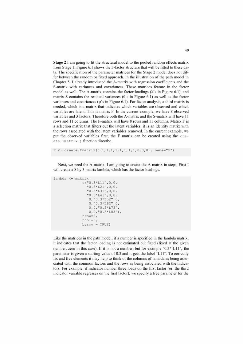
69

Stage 2 I am going to fit the structural model to the pooled random effects matrix

from Stage 1. Figure 6.1 shows the 3-factor structure that will be fitted to these da-

ta. The specification of the parameter matrices for the Stage 2 model does not dif-

fer between the random or fixed approach. In the illustration of the path model in

Chapter 5, I already introduced the A-matrix with regression coefficients and the

S-matrix with variances and covariances. These matrices feature in the factor

model as well. The A-matrix contains the factor loadings (λ’s in Figure 6.1), and

matrix S contains the residual variances (θ’s in Figure 6.1) as well as the factor

variances and covariances (φ’s in Figure 6.1). For factor analysis, a third matrix is

needed, which is a matrix that indicates which variables are observed and which

variables are latent. This is matrix F. In the current example, we have 8 observed

variables and 3 factors. Therefore both the A-matrix and the S-matrix will have 11

rows and 11 columns. The F-matrix will have 8 rows and 11 columns. Matrix F is

a selection matrix that filters out the latent variables, it is an identity matrix with

the rows associated with the latent variables removed. In the current example, we

put the observed variables first, the F matrix can be created using the cre-

ate.Fmatrix() function directly:

F <- create.Fmatrix(c(1,1,1,1,1,1,1,1,0,0,0), name="F")

Next, we need the A-matrix. I am going to create the A-matrix in steps. First I

will create a 8 by 3 matrix lambda, which has the factor loadings.

lambda <- matrix(

c("0.3*L11",0,0,

"0.3*L21",0,0,

"0.3*L31",0,0,

"0.3*L41",0,0,

0,"0.3*L52",0,

0,"0.3*L62",0,

0,0,"0.3*L73",

0,0,"0.3*L83"),

nrow=8,

ncol=3,

byrow = TRUE)

Like the matrices in the path model, if a number is specified in the lambda matrix,

it indicates that the factor loading is not estimated but fixed (fixed at the given

number, zero in this case). If it is not a number, but for example "0.3* L11", the

parameter is given a starting value of 0.3 and it gets the label “L11”. To correctly

fix and free elements it may help to think of the columns of lambda as being asso-

ciated with the common factors and the rows as being associated with the indica-

tors. For example, if indicator number three loads on the first factor (or, the third

indicator variable regresses on the first factor), we specify a free parameter for the

70

element in the third row, first column ("0.3*L31"). Note that the matrix() func-

tion fills in the values column wise by default, so we use the argument byrow =

TRUE. The object lambda looks like shown below.

> lambda

[,1] [,2] [,3]

[1,] "0.3*L11" "0" "0"

[2,] "0.3*L21" "0" "0"

[3,] "0.3*L31" "0" "0"

[4,] "0.3*L41" "0" "0"

[5,] "0" "0.3*L52" "0"

[6,] "0" "0.3*L62" "0"

[7,] "0" "0" "0.3*L73"

[8,] "0" "0" "0.3*L83"

The A-matrix should be an 11 by 11 matrix, in which the factor loadings are in

rows 1 to 8 (associated with the observed variables) and columns 9 to 11 (associ-

ated with the factors). The rest of the matrix should consist of zeros, as there are

no other regression coefficients than factor loadings in the model. The zeros can

be added to the A matrix by adding a 8 by 8 matrix to the left of lambda and con-

sequently a 3 by 11 matrix with zeros below using the cbind() and rbind()

functions. Next, the as.mxMatrix() function is used to create the matrices that

are used by OpenMx, which are a matrix indicating the labels of the parameters, a

matrix with the starting values of the parameters and a matrix indicating whether

the parameter is freely estimated (indicated by TRUE) or not (indicated by FALSE).

A <- rbind(cbind(matrix(0,ncol=8,nrow=8),lambda),

matrix(0, nrow=3, ncol=11))

A <- as.mxMatrix(A)

# not required but it helps to provide labels

dimnames(A) <- list(

c("face","pict","faci","sens","chen","blen","emma","emre","F1

","F2","F3"),

c("face","pict","faci","sens","chen","blen","emma","emre","F1

","F2","F3"))

The resulting A-matrices look as follows.

FullMatrix 'A'

$labels

face pict faci sens chen blen emma emre F1 F2 F3

face NA NA NA NA NA NA NA NA "L11" NA NA

pict NA NA NA NA NA NA NA NA "L21" NA NA

faci NA NA NA NA NA NA NA NA "L31" NA NA

sens NA NA NA NA NA NA NA NA "L41" NA NA

71

chen NA NA NA NA NA NA NA NA NA "L52" NA

blen NA NA NA NA NA NA NA NA NA "L62" NA

emma NA NA NA NA NA NA NA NA NA NA "L73"

emre NA NA NA NA NA NA NA NA NA NA "L83"

F1 NA NA NA NA NA NA NA NA NA NA NA

F2 NA NA NA NA NA NA NA NA NA NA NA

F3 NA NA NA NA NA NA NA NA NA NA NA

$values

face pict faci sens chen blen emma emre F1 F2 F3

face 0 0 0 0 0 0 0 0 0.3 0.0 0.0

pict 0 0 0 0 0 0 0 0 0.3 0.0 0.0

faci 0 0 0 0 0 0 0 0 0.3 0.0 0.0

sens 0 0 0 0 0 0 0 0 0.3 0.0 0.0

chen 0 0 0 0 0 0 0 0 0.0 0.3 0.0

blen 0 0 0 0 0 0 0 0 0.0 0.3 0.0

emma 0 0 0 0 0 0 0 0 0.0 0.0 0.3

emre 0 0 0 0 0 0 0 0 0.0 0.0 0.3

F1 0 0 0 0 0 0 0 0 0.0 0.0 0.0

F2 0 0 0 0 0 0 0 0 0.0 0.0 0.0

F3 0 0 0 0 0 0 0 0 0.0 0.0 0.0

$free

face pict faci sens chen blen emma emre F1 F2 F3

face FALSE FALSE FALSE FALSE FALSE FALSE FALSE FALSE TRUE FALSE FALSE

pict FALSE FALSE FALSE FALSE FALSE FALSE FALSE FALSE TRUE FALSE FALSE

faci FALSE FALSE FALSE FALSE FALSE FALSE FALSE FALSE TRUE FALSE FALSE

sens FALSE FALSE FALSE FALSE FALSE FALSE FALSE FALSE TRUE FALSE FALSE

chen FALSE FALSE FALSE FALSE FALSE FALSE FALSE FALSE FALSE TRUE FALSE

blen FALSE FALSE FALSE FALSE FALSE FALSE FALSE FALSE FALSE TRUE FALSE

emma FALSE FALSE FALSE FALSE FALSE FALSE FALSE FALSE FALSE FALSE TRUE

emre FALSE FALSE FALSE FALSE FALSE FALSE FALSE FALSE FALSE FALSE TRUE

F1 FALSE FALSE FALSE FALSE FALSE FALSE FALSE FALSE FALSE FALSE FALSE

F2 FALSE FALSE FALSE FALSE FALSE FALSE FALSE FALSE FALSE FALSE FALSE

F3 FALSE FALSE FALSE FALSE FALSE FALSE FALSE FALSE FALSE FALSE FALSE

$lbound: No lower bounds assigned.

$ubound: No upper bounds assigned.

The S-matrix with variances and covariances will also be created in steps. It ac-

tually consists of a variance covariance matrix of the observed variables and a var-

iance covariance matrix of the factors. First, I am going to create the matrix with

the residual variances of the observed variables. These are represented by θ’s in

Figure 6.1. The matrix theta is an 8 by 8 matrix, with freely estimated parameters

on its diagonal. As there are no residual covariances in the model, all off-diagonal

elements are fixed at zero. First, I create an 8 by 8 matrix with zero’s, and then I

add the vector with the information about the residual variance on its diagonal.

theta <- matrix(0,nrow = 8,ncol = 8)

diag(theta) <- c("0.1*t11","0.1*t22","0.1*t33","0.1*t44",

"0.1*t55","0.1*t66","0.1*t77","0.1*t88")

The phi matrix contains the variances and covariances of the factors. For identifi-

cation, the factor variances are fixed at 1. The correlations between the factors are

specified off-diagonal.

72

phi <- matrix(

c(1,"0.1*phi21","0.1*phi31",

"0.1*phi21",1,"0.1*phi32",

"0.1*phi31","0.1*phi32",1),

nrow = 3,

ncol = 3)

The function bdiagMat() creates the larger S-matrix from the theta and phi ma-

trices. By using the as.MxMatrix() function on this S-matrix, the matrices with

labels, starting values and free/fixed elements to be used by OpenMx are created.

S <- bdiagMat(list(theta, phi))

S <- as.mxMatrix(S)

dimnames(S) <- list(

c("face","pict","faci","sens","chen","blen","emma","emre","F1

","F2","F3"),

c("face","pict","faci","sens","chen","blen","emma","emre","F1

","F2","F3"))

The resulting S-matrices look like below.

FullMatrix 'S'

$labels

face pict faci sens chen blen emma emre F1 F2 F3

face "t11" NA NA NA NA NA NA NA NA NA NA

pict NA "t22" NA NA NA NA NA NA NA NA NA

faci NA NA "t33" NA NA NA NA NA NA NA NA

sens NA NA NA "t44" NA NA NA NA NA NA NA

chen NA NA NA NA "t55" NA NA NA NA NA NA

blen NA NA NA NA NA "t66" NA NA NA NA NA

emma NA NA NA NA NA NA "t77" NA NA NA NA

emre NA NA NA NA NA NA NA "t88" NA NA NA

F1 NA NA NA NA NA NA NA NA NA "phi21" "phi31"

F2 NA NA NA NA NA NA NA NA "phi21" NA "phi32"

F3 NA NA NA NA NA NA NA NA "phi31" "phi32" NA

$values

face pict faci sens chen blen emma emre F1 F2 F3

face 0.1 0.0 0.0 0.0 0.0 0.0 0.0 0.0 0.0 0.0 0.0

pict 0.0 0.1 0.0 0.0 0.0 0.0 0.0 0.0 0.0 0.0 0.0

faci 0.0 0.0 0.1 0.0 0.0 0.0 0.0 0.0 0.0 0.0 0.0

sens 0.0 0.0 0.0 0.1 0.0 0.0 0.0 0.0 0.0 0.0 0.0

chen 0.0 0.0 0.0 0.0 0.1 0.0 0.0 0.0 0.0 0.0 0.0

blen 0.0 0.0 0.0 0.0 0.0 0.1 0.0 0.0 0.0 0.0 0.0

emma 0.0 0.0 0.0 0.0 0.0 0.0 0.1 0.0 0.0 0.0 0.0

emre 0.0 0.0 0.0 0.0 0.0 0.0 0.0 0.1 0.0 0.0 0.0

F1 0.0 0.0 0.0 0.0 0.0 0.0 0.0 0.0 1.0 0.1 0.1

F2 0.0 0.0 0.0 0.0 0.0 0.0 0.0 0.0 0.1 1.0 0.1

F3 0.0 0.0 0.0 0.0 0.0 0.0 0.0 0.0 0.1 0.1 1.0

$free

face pict faci sens chen blen emma emre F1 F2 F3

73

face TRUE FALSE FALSE FALSE FALSE FALSE FALSE FALSE FALSE FALSE FALSE

pict FALSE TRUE FALSE FALSE FALSE FALSE FALSE FALSE FALSE FALSE FALSE

faci FALSE FALSE TRUE FALSE FALSE FALSE FALSE FALSE FALSE FALSE FALSE

sens FALSE FALSE FALSE TRUE FALSE FALSE FALSE FALSE FALSE FALSE FALSE

chen FALSE FALSE FALSE FALSE TRUE FALSE FALSE FALSE FALSE FALSE FALSE

blen FALSE FALSE FALSE FALSE FALSE TRUE FALSE FALSE FALSE FALSE FALSE

emma FALSE FALSE FALSE FALSE FALSE FALSE TRUE FALSE FALSE FALSE FALSE

emre FALSE FALSE FALSE FALSE FALSE FALSE FALSE TRUE FALSE FALSE FALSE

F1 FALSE FALSE FALSE FALSE FALSE FALSE FALSE FALSE FALSE TRUE TRUE

F2 FALSE FALSE FALSE FALSE FALSE FALSE FALSE FALSE TRUE FALSE TRUE

F3 FALSE FALSE FALSE FALSE FALSE FALSE FALSE FALSE TRUE TRUE FALSE

$lbound: No lower bounds assigned.

$ubound: No upper bounds assigned.

Now the required matrices for the Stage 2 analysis are created, the model can

be fit to the pooled matrix from Stage 1. As the heterogeneity seems to be substan-

tial, I will fit the model to the Stage 1 matrix from the random effects analysis.

The tssem() function distils the averaged correlation matrix and the asymptotic

variance covariance matrix from the Stage 1 object stage1random. As with the

path model I used the diag.constraints=TRUE and I asked for likelihood

based confidence intervals around the parameter estimates.

stage2_random <- tssem2(stage1random, Amatrix=A, Smatrix=S,

Fmatrix=F, diag.constraints=TRUE, intervals="LB")

The output can be viewed using the summary() function.

95% confidence intervals: Likelihood-based statistic

Coefficients:

Estimate Std.Error lbound ubound

L11 0.53025 NA 0.49697 0.56407

L21 0.51982 NA 0.48654 0.55357

L31 0.57671 NA 0.53907 0.61460

L41 0.58797 NA 0.55268 0.62363

L52 0.67185 NA 0.61658 0.72768

L62 0.63164 NA 0.57877 0.68495

L73 0.65046 NA 0.60409 0.69766

L83 0.68395 NA 0.63626 0.73287

t11 0.71883 NA 0.68182 0.75302

t22 0.72979 NA 0.69356 0.76327

t33 0.66741 NA 0.62227 0.70940

t44 0.65429 NA 0.61108 0.69455

t55 0.54862 NA 0.47047 0.61983

t66 0.60103 NA 0.53084 0.66503

t77 0.57691 NA 0.51325 0.63508

t88 0.53222 NA 0.46289 0.59518

phi21 0.60974 NA 0.55321 0.67299

phi31 0.62987 NA 0.57794 0.68595

phi32 0.66528 NA 0.59029 0.74944

74

Goodness-of-fit indices:

Value

Sample size 10564.0000

Chi-square of target model 42.2013

DF of target model 17.0000

p value of target model 0.0006

Number of constraints imposed on "Smatrix" 8.0000

DF manually adjusted 0.0000

Chi-square of independence model 2486.1537

DF of independence model 28.0000

RMSEA 0.0118

SRMR 0.0257

TLI 0.9831

CFI 0.9897

AIC 8.2013

BIC -115.3073

OpenMx status1: 0 ("0" or "1": The optimization is considered

fine.

Other values indicate problems.)

The 8 by 8 pooled correlation matrix on which the model is fitted contains 28 cor-

relation coefficients. The model contains 8 factor loadings, 8 residual variances,

and 3 factor covariances (factor variances were fixed at 1), which sums up to 19

parameters. However, because during estimation the 8 diagonal elements of the

estimated covariance are constrained to be 1, this reduces the number of parame-

ters by 8. Degrees of freedom are therefore equal to 28 – 19 + 8 = 17. The model

does not fit exactly, as the chi-square is significant (χ2(17) = 42.20, p < .05). The

RMSEA value of .012 indicates close approximate fit, and the CFI of .99 also in-

dicated satisfactory fit of the model. The parameter estimates with the confidence

intervals could therefore be interpreted. All factor loadings are positive, larger

than .50, and significantly larger than zero. The correlations between the three fac-

tors is substantial (.62 , .64 and .67), but not so large that some factors may be re-

dundant. Figure 6.2 shows the graphical model with the parameter estimates.

75

Figure 6.2 Factor model on the MSCEIT with parameter estimates and 95% con-

fidence intervals.

As long as there are no mediating variables in the model, an alternative to using

the argument diag.constraints=TRUE in the tssem2() function is to use di-

ag.constraints=FALSE (or to leave out this argument). This will lead to the

same fit results and parameter estimates, but the way the analysis is performed is

different. Without the diagonal constraints, the diagonals are totally left out of the

analysis (the diagonal entries are not counted as observations), and no residual

variances (Θ) are estimated. Because a correlation matrix is analyzed, we know

that the total variance of each indicator equals 1. The residual variances can there-

fore be calculated from the matrix with estimated factor loadings (Λ) and matrix

with estimated factor variances and covariances (Φ) using Θ = I – diag(ΛΦΛT),

where I is an 8 by 8 identity matrix.

References

Fan, H., Jackson, T., Yang, X., Tang, W., & Zhang, J. (2010). The factor structure

of the Mayer–Salovey–Caruso Emotional Intelligence Test V2.0

(MSCEIT): A meta-analytic structural equation modeling approach. Per-

sonality and Individual Differences, 48(7), 781-785.

Faces Pictures Facilitation Sensations Changes BlendsEmotional

managemt.

Emotional

relations

Perception of

emotions

Understanding

emotions

Managing

emotions

.72

[.68;.75]

.73

[.69;.76]

.67

[.62;.71]

.65

[.61;.69]

.55

[.47;.62].60

[.53;.67].58

[.51;.64]

.53

[.46;.60]

.53

[.50;.56] .52

[.49;.55] .58

[.54;.61]

.59

[.55;.62].67

[.62;.73]

.63

[.58;.68].65

[.60;.70]

.68

[.63;.73]

1 11

.61

[.55;.67]

.63

[.58;.69]

.67

[.59;.75]

76

Salovey, P., & Mayer, J. D. (1989). Emotional intelligence. Imagination, cogni-

tion and personality, 9(3), 185-211.

Acknowledgement

I am grateful to dr. Huiyong Fan and the co-authors of his study for sharing the

collected correlation matrices with me. Indirectly, I am also grateful to the authors

of the primary studies, who were willing to share their correlation matrices with

them. I would like to stress that the ownership of these data belongs to the primary

authors. I put the file with the correlation matrices on my website for educational

purposes. Any part of these data should not be used for other purpose than re-

search or education, without prior written permission from these primary authors

or Dr. Huiyong Fan.

Appendix A

Model implied covariance matrix of the example path model

And the model implied variance of Variable 4 (didn’t fit in the matrix above)

Appendix B

Fitting a path model to a covariance matrix with OpenMx

In this appendix I explain how to fit the path model from Chapter 1 to a covari-

ance matrix. I assume that you understand the basics of R. There exist different

approaches to fit models using OpenMx. I will use the matrix based approach.

Another way would be to use the “path model specification”.

To get started with OpenMx you first download the package ‘OpenMx’. With the

command:

source('http://openmx.psyc.virginia.edu/getOpenMx.R')

the latest version of the package ‘OpenMx’ will be downloaded from the OpenMx

website. You have to do this only the first time you use OpenMx (on a specific

computer), to add the package to the R library. To activate the package into the

current R workspace, you type

require(OpenMx)

A script to fit a path model with OpenMx consists of four steps. First, the ob-

served covariance matrix has to be specified in R. Second, the model has to be

specified. Third, we fit the model to the observed covariance matrix, by submit-

ting both model and covariance matrix to OpenMx. Finally, the output needs to be

retrieved from the object where all results are stored.

The script below fits the path model from Chapter 1 to a covariance matrix. All

commands will be explained afterwards.

source('http://openmx.psyc.virginia.edu/getOpenMx.R')

require(OpenMx)

# observed covariance matrix

obsnames <- c("pos","neg","enga","achiev")

obslabels <- list(obsnames,obsnames)

obscov <- matrix(c(.81,-.36,.63,.14,

-.36,1.21,-.60,-.33,

.63,-.60,1.69,.50,

.14,-.33,.50,1.44),

nrow = 4, ncol = 4,

dimnames = obslabels)

80

# define the model

title <- "Path model"

obs <- mxData(observed = obscov, type = "cov", numObs =

104)

matrixB <- mxMatrix(

type = "Full",

nrow = 4,

ncol = 4,

free = c(FALSE,FALSE,FALSE,FALSE,

FALSE,FALSE,FALSE,FALSE,

TRUE,TRUE,FALSE,FALSE,

FALSE,FALSE,TRUE,FALSE),

values = c(0,0,0,0,

0,0,0,0,

1,1,0,0,

0,0,1,0),

labels = c(NA,NA,NA,NA,

NA,NA,NA,NA,

"b31","b32",NA,NA,

NA,NA,"b43",NA),

byrow = TRUE,

name = "B",

dimnames = obslabels)

matrixP <- mxMatrix(

type = "Symm",

nrow = 4,

ncol = 4,

free = c(TRUE,

TRUE,TRUE,

FALSE,FALSE,TRUE,

FALSE,FALSE,FALSE,TRUE),

values = c(1,

.5,1,

0,0,1,

0,0,0,1),

byrow = TRUE,

name = "P",

dimnames = obslabels)

81

matrixI <- mxMatrix(

type = "Iden",

nrow = 4,

ncol = 4,

name = "I")

Ind_pos <- mxAlgebra(expression = "b31"*"b43",

name = "Ind_pos")

Ind_neg <- mxAlgebra(expression = "b32"*"b43",

name = "Ind_neg")

conf <- mxCI(c("B","P","Ind_pos","Ind_neg"),interval = .95)

algebraS <- mxAlgebra(expression =

solve(I-B) %*% P %*% t(solve(I-B)),

name = "Sigma", dimnames = obslabels)

exp <- mxExpectationNormal(covariance="Sigma")

fit <- mxFitFunctionML()

pathmodel<- mxModel(title,obs,matrixB,matrixP,matrixI,

Ind_pos,Ind_neg,conf,algebraS,exp,fit)

pathmodelOut <- mxRun(pathmodel, intervals = TRUE)

# retrieve the output

summary(pathmodelOut)

pathmodelOut$B@values

pathmodelOut$P@values

We start by defining the observed covariance matrix and the labels (names) of the

associated observed variables. It is required to provide these labels with the input

matrix. The labels are given as a list with two elements, one vector of row names

and one vector of column names. First we created the object obsnames with the

names of the variables.

obsnames <- c("pos","neg","enga","achiev")

obslabels <- list(obsnames,obsnames)

The observed covariance matrix is stored in the object obscov, by creating a ma-

trix with the values of the elements, number of rows, number of columns, and the

name vectors of the two dimensions.

obscov <- matrix()

82

To check whether you successfully specified the observed covariance matrix,

check the results by typing obscov in the R console. And check, for example,

whether the matrix is indeed symmetrical by typing obscov == t(obscov).

The next step is to specify the model that has to be fitted to the observed data. The

OpenMx package has several functions that we will use. The main functions are

mxModel()and mxRun(). mxModel() is a ‘container-function’ that results in an

object that contains all the information needed to fit the model. The model is actu-

ally fitted with the mxRun() function. All parts of the model fitting process are

first created as separate objects, and then stored in another object using the

mxModel() function. The different objects are:

- A title

- The data (e.g. observed covariance matrix)

- The matrices containing the model parameters

- The expected (model implied) covariance matrix and fit-function

The code

title <- "Path model"

defines an object with the title, do not forget the " " to make the object of the type

character (i.e., so R knows that title is a line of text, not a number).

obs <- mxData(observed = obscov, type = "cov",

numObs = 104)

This line creates the object obs to store the outcome of the function mxData().

The function mxData() has three arguments: 1) observed = for the observed

matrix (that you specified previously), 2) type = for the type of the matrix

("cor" for correlation matrix, and "cov" for covariance matrix), and 3) numObs =

for the number of observations, the sample size.

The model implied covariance matrix of a path model is as follows:

Σ = (I - Β)-1 * Ψ * (I - Β)-1t, (C.1)

where Σ is the matrix with the resulting model implied variances and covariances,

I is an identity matrix, Β is a matrix containing the direct effects, and Ψ is a matrix

containing variances and covariances. In openMx we will denote Σ, Β, Ψ and I

with respectively Sigma, B, P and I.

matrixB <- mxMatrix(

type = "Full",

nrow = 4,

ncol = 4,

83

free = c(FALSE,FALSE,FALSE,FALSE,

FALSE,FALSE,FALSE,FALSE,

TRUE,TRUE,FALSE,FALSE,

FALSE,FALSE,TRUE,FALSE),

values = c(0,0,0,0,

0,0,0,0,

1,1,0,0,

0,0,1,0),

labels = c(NA,NA,NA,NA,

NA,NA,NA,NA,

"b31","b32",NA,NA,

NA,NA,"b43",NA),

byrow = TRUE,

name = "B",

dimnames = obslabels)

Matrix B contains the parameters for the direct effects. Matrix B is constructed us-

ing the function mxMatrix() with several arguments. B is a full matrix (type =

"Full"), with numbers of rows and columns equal to the number of observed

variables. The argument

free = c(FALSE,FALSE,FALSE,FALSE,

FALSE,FALSE,FALSE,FALSE,

TRUE,TRUE,FALSE,FALSE,

FALSE,FALSE,TRUE,FALSE),

is a vector (in matrix shape) specifying which elements in matrix B should be es-

timated (TRUE) and which should not be estimated (FALSE). Both the rows and

the columns of the B matrix are associated with the (four) observed variables.

You need to be careful to specify these direct effects correctly. It may help to

realize that the columns are associated with the independent variables, and the

rows with the dependent variables. Another way to think about it is to formulate in

terms of regression: when Variable 4 is regressed on Variable 1, you specify TRUE

in element B 4 1. The diagonal of B is always FALSE, as a variable cannot be re-

gressed on itself. The argument

values = c(0,0,0,0,

0,0,0,0,

1,1,0,0,

0,0,1,0),

is a vector of values. These values are fixed values for the fixed (FALSE) elements

(usually zero), or start values for the parameters to be estimated (TRUE). To speci-

84

fy a start value for the direct effect of Variable 1 on Variable 4, or regression of

Variable 4 on Variable 1 (β41), we put a 1 (or some other value) in row 4, column

1 of the B matrix. The parameters can be given labels, which are for example

needed if you want to calculate indirect effects or add equality constraints later on,

by adding:

labels = c(NA,NA,NA,NA,

NA,NA,NA,NA,

"b31","b32",NA,NA,

NA,NA,"b43",NA),

The argument:

byrow = TRUE,

name = "B",

dimnames = obslabels)

should not be forgotten, because the matrix should be filled with elements by row

and not by column (which is the default). The matrix is given a name (“B”) that

can be used within other parts of the mxModel. The last argument provides labels

to the rows and columns of the matrix.

matrixP <- mxMatrix(

type = "Symm",

nrow = 4,

ncol = 4,

free = c(TRUE,

TRUE,TRUE,

FALSE,FALSE,TRUE,

FALSE,FALSE,FALSE,TRUE),

values = c(1,

.5,1,

0,0,1,

0,0,0,1),

byrow = TRUE,

name = "P",

dimnames = obslabels)

Matrix P is also an mxMatrix and contains the variances and covariances between

variables (or between disturbances for endogenous variables). P is a symmetrical

matrix (type = "Symm") with the same dimensions as the B matrix (i.e., the

number of observed variables). The free elements in the P matrix are provided in a

symmetrical matrix with FALSE for fixed elements, and TRUE for free to be esti-

mated elements. In this example there are TRUE’s on the diagonal, meaning that

the variances of the exogenous variables and the disturbance variances of the en-

85

dogenous variables are free to be estimated. Off diagonal there is only one TRUE,

for the covariance between the two exogenous variables (The double headed ar-

row between “Positive relations” and “Negative relations” in Chapter 1).

matrixI <- mxMatrix(

type = "Iden",

nrow = 4,

ncol = 4,

name = "I")

Matrix I is an identity matrix (type = “Iden”), with the same dimensions as

the B and P matrices (i.e., the number of observed variables). It needs fewer ar-

guments, because all elements of an identity matrix are fixed.

Ind_pos <- mxAlgebra(expression = "b31"*"b43",

name = "Ind_pos")

Ind_neg <- mxAlgebra(expression = "b32"*"b43",

name = "Ind_neg")

The indirect effects from Negative and Positive interactions on Achievement,

through Engagement, are calculated in an mxAlgebra() function, by referring to

the labels of the two direct effects that make up the indirect effect.

conf <- mxCI(c("B","P","Ind_pos","Ind_neg"),

interval = .95)

With the mxCI() function we ask for 95% likelihood based confidence intervals

for all elements in the B and P matrices, and the indirect effects.

algebraS <- mxAlgebra(expression =

solve(I-B) %*% P %*% t(solve(I-B)),

name = "Sigma", dimnames = obslabels)

The model implied covariance matrix is defined in algebraS, with the mxAlge-

bra() function, using the matrices that have been defined before in the expression

of the path model. We name this model implied matrix “Sigma”. The model im-

plied covariance matrix is given the same labels as the observed covariance matrix

through dimnames = obslabels.

exp <- mxExpectationNormal(covariance="Sigma")

fit <- mxFitFunctionML()

The mxMLObjective() function has as arguments the model implied covariance

matrix. The mxFitFunctionML() function does not need arguments, but has to

be added to the mxModel to indicate that we want to use the maximum likelihood

86

fit function. Now, all separate elements of an mxModel are created, and we can

build the actual mxModel, calling it ‘pathmodel’:

pathmodel <- mxModel(title,obs,matrixB,matrixP,

matrixI,Ind_pos,Ind_neg,conf,algebraS,exp,fit)

We actually fit (“run”) the model by specifying mxRun(pathmodel)and store the

output in ‘pathmodelOut’:

pathmodelOut <- mxRun(pathmodel, intervals = TRUE)

The intervals = TRUE argument can be used to specify whether the confidence

intervals should be estimated or not. For very large models it may take a long time

to estimate the intervals so the argument may be set to FALSE in some cases.

In order to get information about the model fit and parameter estimates, we can

ask for a summary of the output:

summary(pathmodelOut)

In the summary, one will see the observed covariance matrix, the parameter esti-

mates with standard errors and some of the fit results. This model has 2 degrees of

freedom, and a chi-square of 2.538.

Information about the parameter estimates only, in matrix shape can be obtained

with: pathmodelOut$B$values

pathmodelOut$P$values

87

Appendix C

Model implied covariance matrix of the example factor model

88

Appendix D

Fitting a factor model to a covariance matrix with OpenMx

The openMx script for fitting a factor model resembles the script for fitting a path

model. The biggest difference is that the model of Σ is now a factor model:

Σ = Λ Φ Λ’+ Θ, (D.1)

where Λ is a full matrix with factor loadings, Φ is a symmetric matrix with vari-

ances and covariances of the common factors, and Θ is a diagonal matrix with

variances (or sometimes a symmetric matrix with covariances) of the residual fac-

tors.

The script below fits the two-factor model depicted in Chapter 1, to the observed

covariance matrix.

# observed covariance matrix

obsnames <- c("with","somat","anxiety","delinq","aggres")

factornames <- c('Internalizing','Externalizing')

obslabels <- list(obsnames,obsnames)

factorlabels <- list(factornames,factornames)

lambdalabels <- list(obsnames,factornames)

CBCLcov <- matrix(c(12.554, 6.306,11.147, 2.846,12.437,

6.306,10.057, 9.642, 2.090, 9.679,

11.147, 9.642,26.018, 4.836,22.199,

2.846, 2.090, 4.836, 3.718, 9.962,

12.437, 9.679,22.199,9.962, 51.020),

nrow = 5, ncol = 5,

dimnames = obslabels)

# Model

title <- "Factor model CBCL"

obs <- mxData(observed = CBCLcov, type = "cov",

numObs = 155)

matrixL <- mxMatrix(

type = "Full",

nrow = 5,

ncol = 2,

free = c(FALSE,FALSE,

TRUE,FALSE,

TRUE,FALSE,

FALSE,FALSE,

89

FALSE,TRUE),

values = c(1,0,

1,0,

1,0,

0,1,

0,1),

byrow = TRUE,

name = "L",

dimnames = list(obsnames,factornames))

matrixF <- mxMatrix(

type = "Symm",

nrow = 2,

ncol = 2,

free = c(TRUE,

TRUE,TRUE),

values = c(1,

.5,1),

byrow = TRUE,

name = "F",

dimnames = factorlabels)

matrixT <- mxMatrix(

type = "Diag",

nrow = 5,

ncol = 5,

free = c(TRUE,TRUE,TRUE,TRUE,TRUE),

values = c(1,1,1,1,1),

byrow = TRUE,

name = "T",

dimnames = obslabels)

conf <- mxCI(c("L","F","T"),interval = .95)

algebraS <- mxAlgebra(expression = L%*%F%*%t(L) + T, name =

"Sigma", dimnames = obslabels)

exp <- mxExpectationNormal(covariance="Sigma")

fit <- mxFitFunctionML()

CBCLmodel <- mxModel(title,obs,matrixL,matrixF,matrixT,

conf,algebraS,exp,fit)

90

CBCLmodelOut <- mxRun(CBCLmodel)

# retrieve the output

summary(CBCLmodelOut)

CBCLmodelOut$L$values

CBCLmodelOut$F$values

CBCLmodelOut$T$values

The first part of the script, where the observed covariance matrix is created, is not

different from when fitting a path model. Differences are present in the matrices

that are used. The matrices involved in a factor model are Λ, Φ and Θ. In openMx

we will use L, F, and Q to denote Λ , Φ , and Θ, respectively.

To facilitates reading the results in the L, F and Q matrix, we now need both the

names of the observed variables and the common factors. Therefore, we also cre-

ated an object with the names of the common factors:

factornames <- c('Internalizing','Externalizing')

And we create the lists with the labels for the matrices in the factormodel:

obslabels <- list(obsnames,obsnames)

factorlabels <- list(factornames,factornames)

lambdalabels <- list(obsnames,factornames)

The labels of the Lambda matrix involve both the names of the observed variables

(the rows) and the names of the common factors (the columns).

Matrix L contains the factor loadings. Factor loadings are the regression coeffi-

cients for the regressions of the indicator variables on the common factors (i.e., the

effects of the factors on the indicator variables). L is always a full matrix, with the

number of rows equal to the number of indicators and the number of columns

equal to the number of common factors.

The argument

free = c(FALSE,FALSE,

TRUE,FALSE,

TRUE,FALSE,

FALSE,FALSE,

FALSE,TRUE),

specifies which factor loadings should be estimated and which are fixed. To cor-

rectly fix and free elements, it may help to think of the columns as being associat-

ed with the common factors and the rows as being associated with the indicators.

91

For example if indicator number three loads on the first factor (or, the third indica-

tor variable regresses on the first factor), we specify TRUE for element (3,1). Start

values and fixed values are provided in the same way as with a path model. In this

example, the first factor loading per factor is fixed to 1 to give the factors a scale.

The alternative would be to fix the variances of the factors to 1.

values = c(1,0,

1,0,

1,0,

0,1,

0,1),

For start values of the free loadings, we used 1.

Matrix F contains the variances and covariances of the common factors. As it is a

covariance matrix, it is always a symmetric matrix. Its dimensions are equal to the

number of common factors. Because we fixed one factor loading per factor at 1 in

this example, the factor variances can be estimated. The TRUE at the off diagonal

indicates that the covariance between the common factors is free to be estimated.

So there is a TRUE for all elements in F. Start values for the elements in F are also

given.

matrixF <- mxMatrix(

type = "Symm",

nrow = 2,

ncol = 2,

free = c(TRUE,

TRUE,TRUE),

values = c(1,

.5,1),

byrow = TRUE,

name = "F",

dimnames = factorlabels)

Matrix T contains the variances of the residual factors. As there are no covariances

between the residual factors, matrix T is a diagonal matrix, with dimensions equal

to the number of indicators. In this example, all residual variance should be esti-

mated, so we provided all TRUE’s in the “free” argument.

matrixT <- mxMatrix(

type = "Diag",

nrow = 5,

ncol = 5,

free = c(TRUE,TRUE,TRUE,TRUE,TRUE),

92

values = c(1,1,1,1,1),

byrow = TRUE,

name = "T",

dimnames = obslabels)

We ask for likelihood based confidence intervals for all parameter estimates:

conf <- mxCI(c("L","F","T"),interval = .95)

The expression for the expected covariance matrix is now a factor model:

algebraS <- mxAlgebra(expression = L%*%F%*%t(L) + Q,

name = "Sigma", dimnames = obslabels)

exp <- mxExpectationNormal(covariance="Sigma")

fit <- mxFitFunctionML()

Finally, all the elements of the model are collected in the mxModel function, and

run with the mxRun function.

CBCLmodel <- mxModel(title,obs,matrixL,matrixF,

matrixT,conf,algebraS,exp,fit)

CBCLmodelOut <- mxRun(CBCLmodel)

The results of the analyses, and the estimates of the L, F and T matrices can be ob-

tained with:

summary(CBCLmodelOut)

CBCLmodelOut$L$values

CBCLmodelOut$F$values

CBCLmodelOut$T$values