Meta-LearningMeta-Learning::towards universal learning paradigmstowards universal learning paradigms

Meta-LearningMeta-Learning::towards universal learning paradigmstowards universal learning paradigms

Włodzisław DuchNorbert Jankowski, Krzysztof Grąbczewski & Co

Department of Informatics, Nicolaus Copernicus University, Toruń, Poland

Google: W. DuchICONIP’09, Bangkok

ToruToruńń

Norbert Tomek Marek KrzysztofNorbert Tomek Marek Krzysztof

CopernicuCopernicuss

Nicolaus Copernicus: born in 1472Nicolaus Copernicus: born in 1472

PlanPlanPlanPlan

• Problems with Computational intelligence (CI)

• What can we learn?• Why solid foundations are needed.• First attempt: similarity based framework for metalearning.• Heterogeneous systems. • Hard boole’an problems and how to solve them.• Projection and transformation-based learning with some

visualization to see how it works.• More components to build algorithms.• Real meta-learning, or algorithms on demand.

What is Computational Intelligence?What is Computational Intelligence?What is Computational Intelligence?What is Computational Intelligence?

The Field of Interest of the Society shall be the theory, design, application, and development of biologically and linguistically motivated computational paradigms emphasizing neural networks, connectionist systems, genetic algorithms, evolutionary programming, fuzzy systems, and hybrid intelligent systems in which these paradigms are contained.Artificial Intelligence (AI) was established in 1956! AI Magazine 2005, Alan Mackworth: In AI's youth, we worked hard to establish our paradigm by vigorously attacking and excluding apparent pretenders to the throne of intelligence, pretenders such as pattern recognition, behaviorism, neural networks, and even probability theory. Now that we are established, such ideological purity is no longer a concern. We are more catholic, focusing on problems, not on hammers. Given that we do have a comprehensive toolbox, issues of architecture and integration emerge as central.

CI definitionCI definitionCI definitionCI definitionComputational Intelligence. An International Journal (1984)+ 10 other journals with “Computational Intelligence”,

D. Poole, A. Mackworth & R. Goebel, Computational Intelligence - A Logical Approach. (OUP 1998), GOFAI book, logic and reasoning.

CI should: • be problem-oriented, not method oriented;• cover all that CI community is doing now, and is likely to do in future;• include AI – they also think they are CI ...

CI: science of solving (effectively) non-algorithmizable problems.

Problem-oriented definition, firmly anchored in computer sci/engineering.AI: focused problems requiring higher-level cognition, the rest of CI is more focused on problems related to perception/action/control.

The future of computational intelligence ...

Wisdom in computers?

What can we learn?What can we learn?What can we learn?What can we learn?Good part of Computational Intelligence is about learning.What can we learn? Everything?

Neural networks are universal approximators and evolutionary algorithms solve global optimization problems – so everything can be learned? Not sufficient! Almost any expansion has universal approximation property.

Duda, Hart & Stork, Ch. 9, No Free Lunch + Ugly Duckling Theorems: • Uniformly averaged over all target functions the expected error for all learning algorithms [predictions by economists] is the same. • Averaged over all target functions no learning algorithm yields generalization error that is superior to any other. • There is no problem-independent or “best” set of features.“Experience with a broad range of techniques is the best insurance for solving arbitrary new classification problems.”In practice: try as many models as you can, rely on your experience and intuition. There is no free lunch, but do we have to cook ourselves?

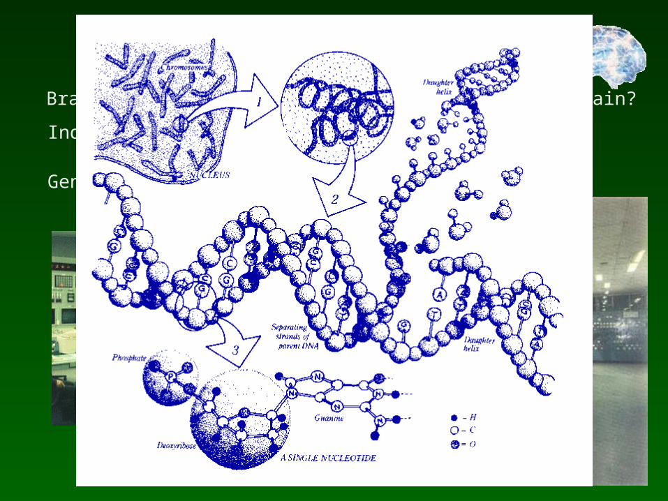
What is there to learn?What is there to learn?What is there to learn?What is there to learn?Brains ... what is in EEG? What happens in the brain?

Industry: what happens?

Genetics, proteins ...

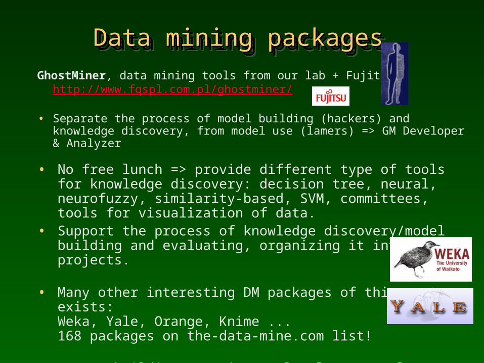
Data mining packagesData mining packagesData mining packagesData mining packages

• No free lunch => provide different type of tools for knowledge discovery: decision tree, neural, neurofuzzy, similarity-based, SVM, committees, tools for visualization of data.

• Support the process of knowledge discovery/model building and evaluating, organizing it into projects.

• Many other interesting DM packages of this sort exists: Weka, Yale, Orange, Knime ... 168 packages on the-data-mine.com list!

• We are building Intemi, completely new tools.

GhostMiner, data mining tools from our lab + Fujitsu: http://www.fqspl.com.pl/ghostminer/

• Separate the process of model building (hackers) and knowledge discovery, from model use (lamers) => GM Developer & Analyzer

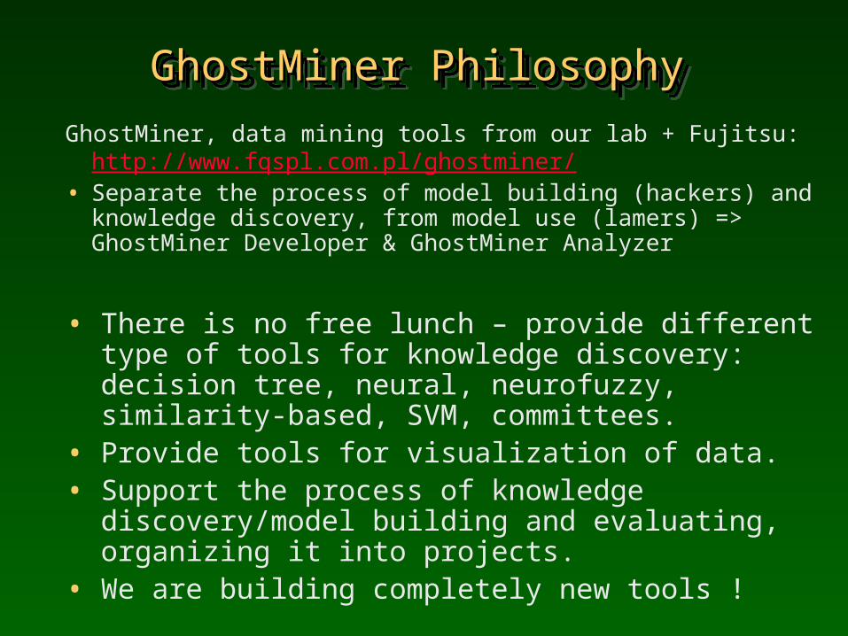
GhostMiner PhilosophyGhostMiner PhilosophyGhostMiner PhilosophyGhostMiner Philosophy

• There is no free lunch – provide different type of tools for knowledge discovery: decision tree, neural, neurofuzzy, similarity-based, SVM, committees.

• Provide tools for visualization of data.• Support the process of knowledge discovery/model building

and evaluating, organizing it into projects.• We are building completely new tools !

Surprise! Almost nothing can be learned using such tools!

GhostMiner, data mining tools from our lab + Fujitsu: http://www.fqspl.com.pl/ghostminer/

• Separate the process of model building (hackers) and knowledge discovery, from model use (lamers) => GhostMiner Developer & GhostMiner Analyzer

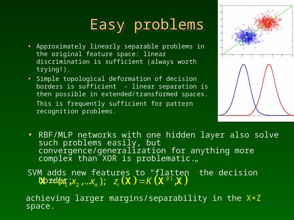
Easy problemsEasy problemsEasy problemsEasy problems• Approximately linearly separable problems in the

original feature space: linear discrimination is sufficient (always worth trying!).

• Simple topological deformation of decision borders is sufficient – linear separation is then possible in extended/transformed spaces. This is frequently sufficient for pattern recognition problems.

• RBF/MLP networks with one hidden layer also solve such problems easily, but convergence/generalization for anything more complex than XOR is problematic.

SVM adds new features to “flatten” the decision border:

( )1 2( , ,... ); ,in ix x x z K X X X X

achieving larger margins/separability in the X+Z space.

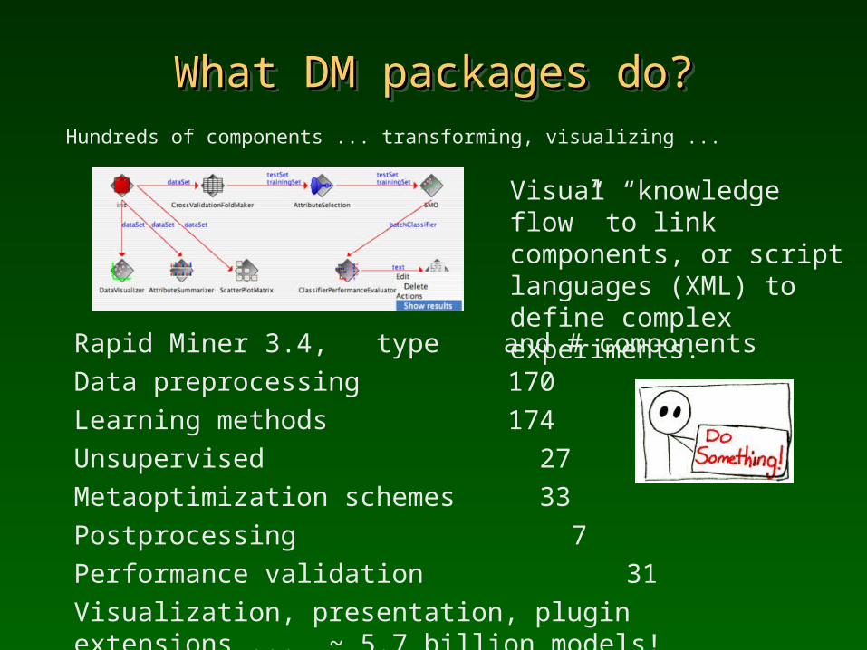
What DM packages do?What DM packages do?What DM packages do?What DM packages do?

Hundreds of components ... transforming, visualizing ...

Rapid Miner 3.4, type and # componentsData preprocessing 170Learning methods 174Unsupervised 27 Metaoptimization schemes 33Postprocessing 7Performance validation 31Visualization, presentation, plugin extensions ... ~ 5.7 billion models!

Visual “knowledge flow” to link components, or script languages (XML) to define complex experiments.

Are we really Are we really so good?so good?

Surprise!

Almost nothing can be learned using such tools!

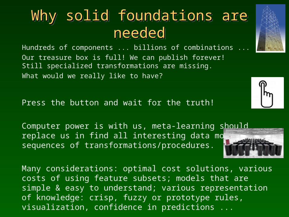
Why solid foundations are neededWhy solid foundations are neededWhy solid foundations are neededWhy solid foundations are needed

Hundreds of components ... billions of combinations ...Our treasure box is full! We can publish forever! Still specialized transformations are missing.What would we really like to have?

Press the button and wait for the truth!

Computer power is with us, meta-learning should replace us in find all interesting data models =sequences of transformations/procedures.

Many considerations: optimal cost solutions, various costs of using feature subsets; models that are simple & easy to understand; various representation of knowledge: crisp, fuzzy or prototype rules, visualization, confidence in predictions ...

Computational Computational

learning learning approach: approach:

let there be let there be light!light!

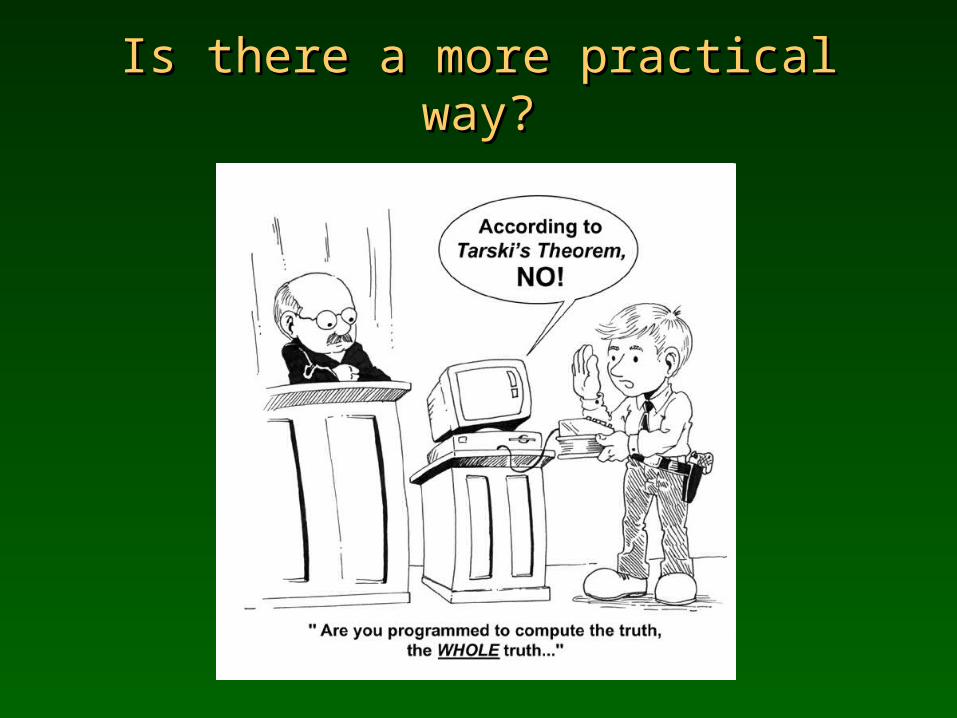
Is there a more practical way?Is there a more practical way?

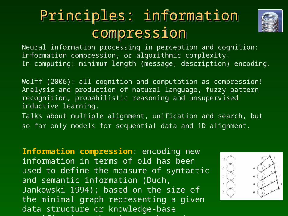
Principles: information compressionPrinciples: information compressionPrinciples: information compressionPrinciples: information compression

Neural information processing in perception and cognition: information compression, or algorithmic complexity. In computing: minimum length (message, description) encoding.

Wolff (2006): all cognition and computation as compression! Analysis and production of natural language, fuzzy pattern recognition, probabilistic reasoning and unsupervised inductive learning.Talks about multiple alignment, unification and search, but so far only models for sequential data and 1D alignment.

Information compression: encoding new information in terms of old has been used to define the measure of syntactic and semantic information (Duch, Jankowski 1994); based on the size of the minimal graph representing a given data structure or knowledge-base specification, thus it goes beyond alignment.

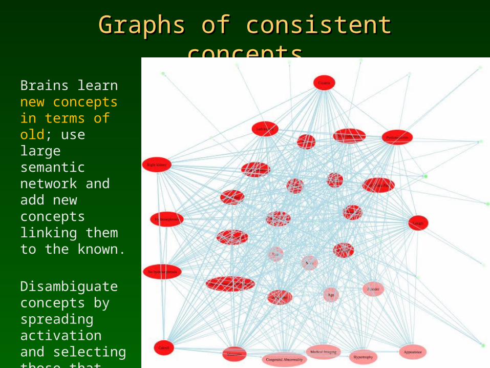
Graphs of consistent conceptsGraphs of consistent concepts

Brains learn new concepts in terms of old; use large semantic network and add new concepts linking them to the known.

Disambiguate concepts by spreading activation and selecting those that are consistent with already active subnetworks.

Making things easy: principlesMaking things easy: principles

Similarity-based frameworkSimilarity-based frameworkSimilarity-based frameworkSimilarity-based framework(Dis)similarity: • more general than feature-based description, • no need for vector spaces (structured objects), • more general than fuzzy approach (F-rules are reduced to P-rules), • includes nearest neighbor algorithms, MLPs, RBFs, separable function

networks, SVMs, kernel methods and many others!

Similarity-Based Methods (SBMs) are organized in a framework: p(Ci|X;M) posterior classification probability or y(X;M) approximators,models M are parameterized in increasingly sophisticated way.

A systematic search (greedy, beam, evolutionary) in the space of all SBM models is used to select optimal combination of parameters and procedures, opening different types of optimization channels, trying to discover appropriate bias for a given problem.

Results: several candidate models are created, even very limited version gives best results in 7 out of 12 Stalog problems.

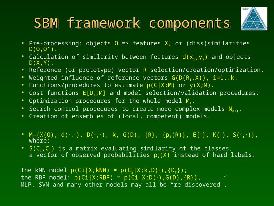
SBM framework componentsSBM framework componentsSBM framework componentsSBM framework components• Pre-processing: objects O => features X, or (diss)similarities D(O,O’). • Calculation of similarity between features d(xi,yi) and objects D(X,Y).• Reference (or prototype) vector R selection/creation/optimization. • Weighted influence of reference vectors G(D(Ri,X)), i=1..k.• Functions/procedures to estimate p(C|X;M) or y(X;M). • Cost functions E[DT;M] and model selection/validation procedures. • Optimization procedures for the whole model Ma.• Search control procedures to create more complex models Ma+1.• Creation of ensembles of (local, competent) models.

• M={X(O), d(.,.), D(.,.), k, G(D), {R}, {pi(R)}, E[.], K(.), S(.,.)}, where:• S(Ci,Cj) is a matrix evaluating similarity of the classes;

a vector of observed probabilities pi(X) instead of hard labels.

The kNN model p(Ci|X;kNN) = p(Ci|X;k,D(.),{DT}); the RBF model: p(Ci|X;RBF) = p(Ci|X;D(.),G(D),{R}), MLP, SVM and many other models may all be “re-discovered”.

Meta-learning in SBM schemeMeta-learning in SBM schemeMeta-learning in SBM schemeMeta-learning in SBM scheme

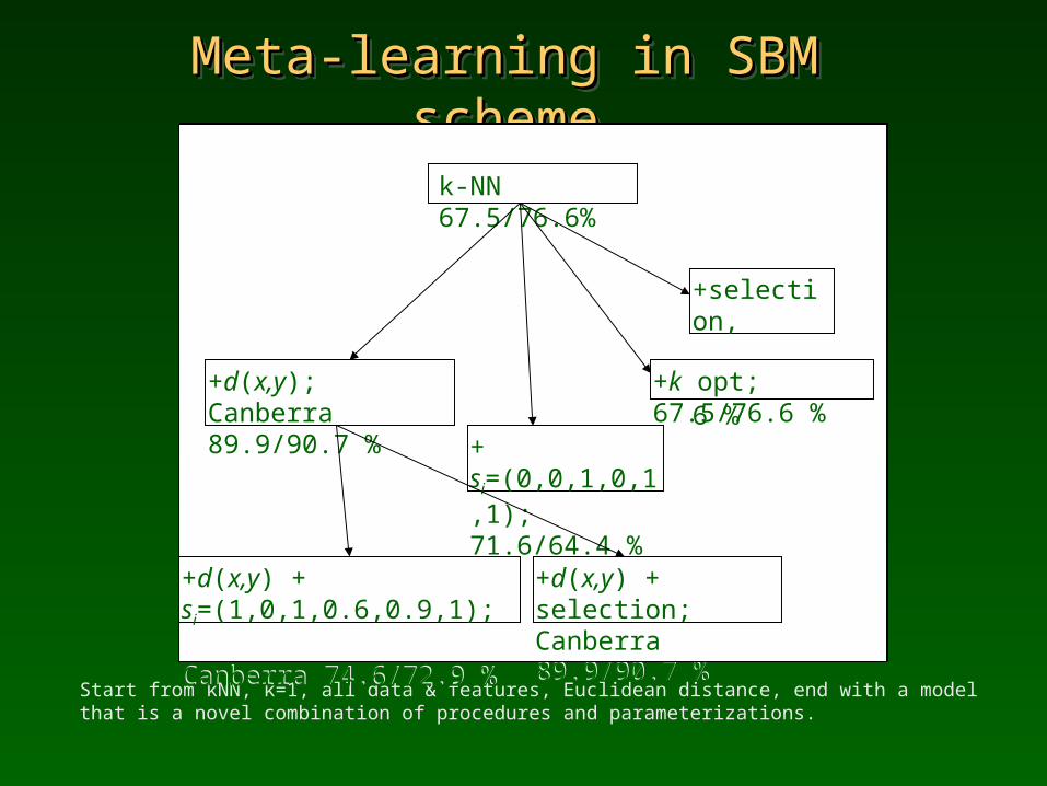
Start from kNN, k=1, all data & features, Euclidean distance, end with a model that is a novel combination of procedures and parameterizations.

k-NN 67.5/76.6%

+d(x,y); Canberra 89.9/90.7 %

+ si=(0,0,1,0,1,1); 71.6/64.4 %

+selection, 67.5/76.6 %

+k opt; 67.5/76.6 %

+d(x,y) + si=(1,0,1,0.6,0.9,1); Canberra 74.6/72.9 %

+d(x,y) + sel. or opt k; Canberra 89.9/90.7 %

k-NN 67.5/76.6%

+d(x,y); Canberra 89.9/90.7 %

+ si=(0,0,1,0,1,1); 71.6/64.4 %

+selection, 67.5/76.6 %

+k opt; 67.5/76.6 %

+d(x,y) + si=(1,0,1,0.6,0.9,1); Canberra 74.6/72.9 %

+d(x,y) + selection; Canberra 89.9/90.7 %

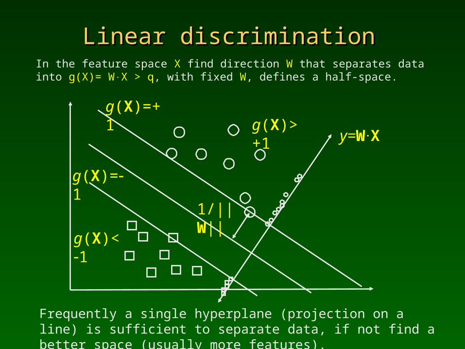
Linear discriminationLinear discriminationIn the feature space X find direction W that separates data into g(X)= WX > q, with fixed W, defines a half-space.

Frequently a single hyperplane (projection on a line) is sufficient to separate data, if not find a better space (usually more features).

1/||W||

g(X)> +1

g(X)< 1

g(X)=+1

g(X)=1

y=W.

X

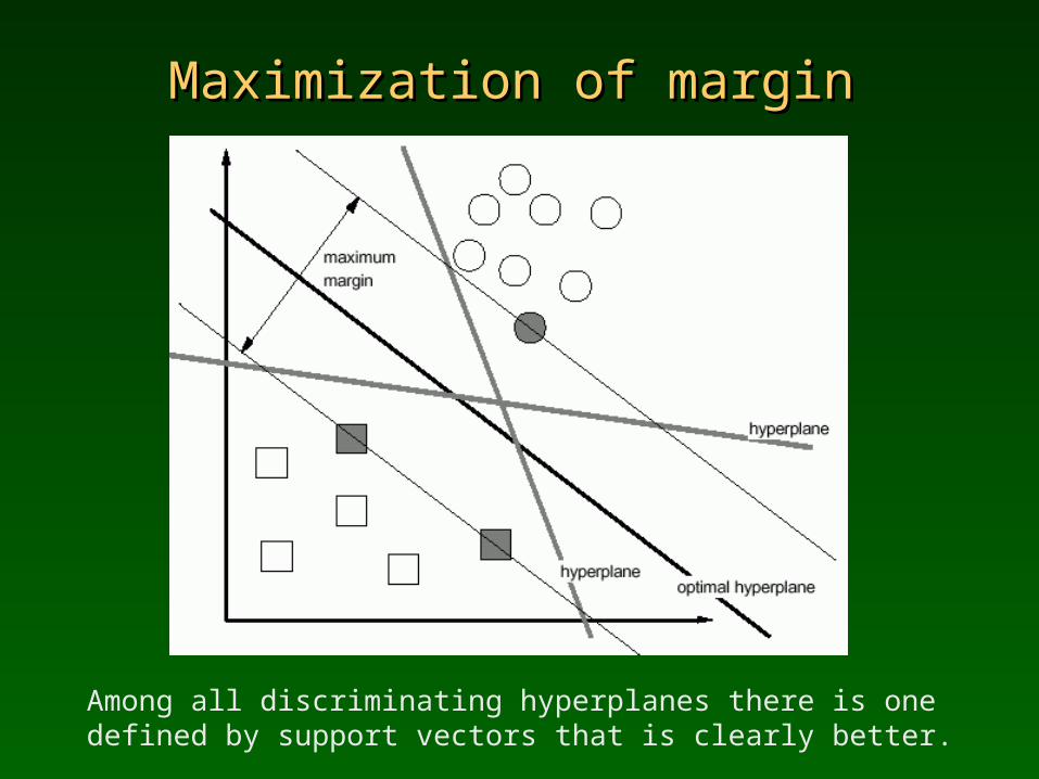
Maximization of marginMaximization of margin

Among all discriminating hyperplanes there is one defined by support vectors that is clearly better.

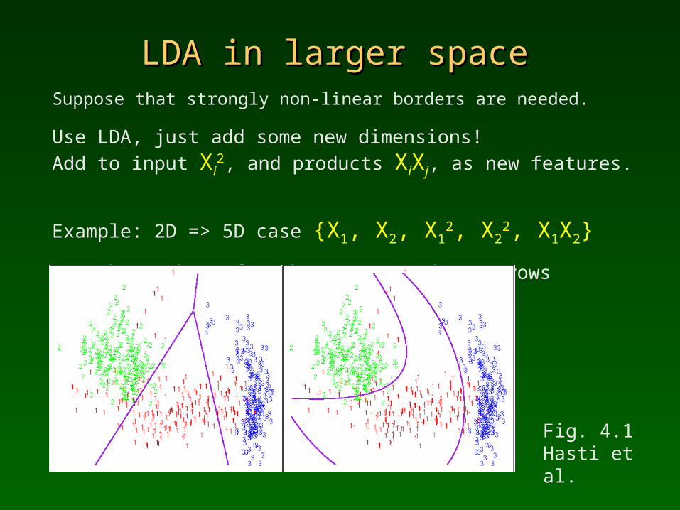
LDA in larger spaceLDA in larger spaceSuppose that strongly non-linear borders are needed.

Use LDA, just add some new dimensions!Add to input Xi

2, and products XiXj, as new features.

Example: 2D => 5D case {X1, X2, X12, X2

2, X1X2}

But the number of such tensor products grows exponentially.

Fig. 4.1Hasti et al.

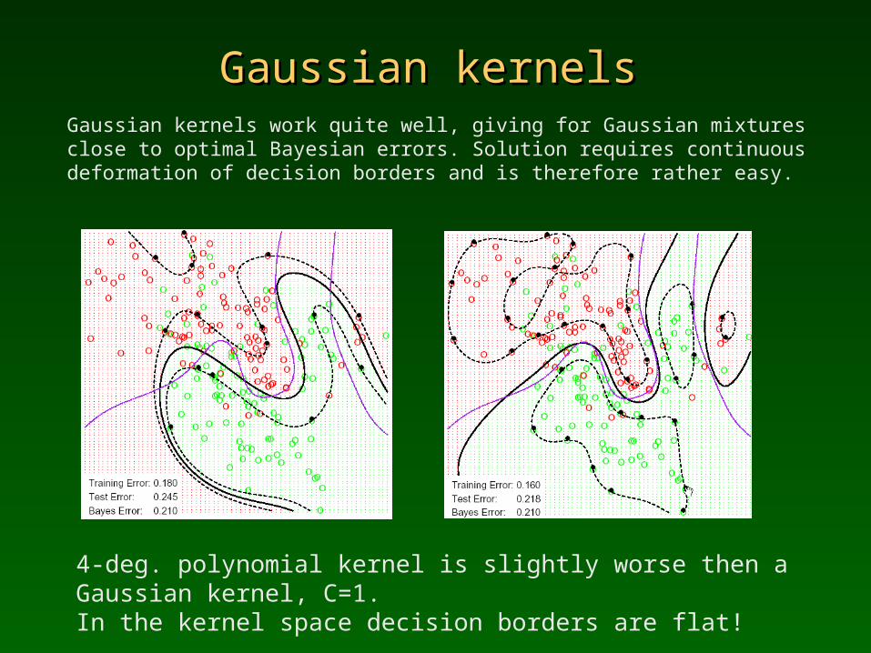
Gaussian kernelsGaussian kernelsGaussian kernels work quite well, giving for Gaussian mixtures close to optimal Bayesian errors. Solution requires continuous deformation of decision borders and is therefore rather easy.

4-deg. polynomial kernel is slightly worse then a Gaussian kernel, C=1.In the kernel space decision borders are flat!

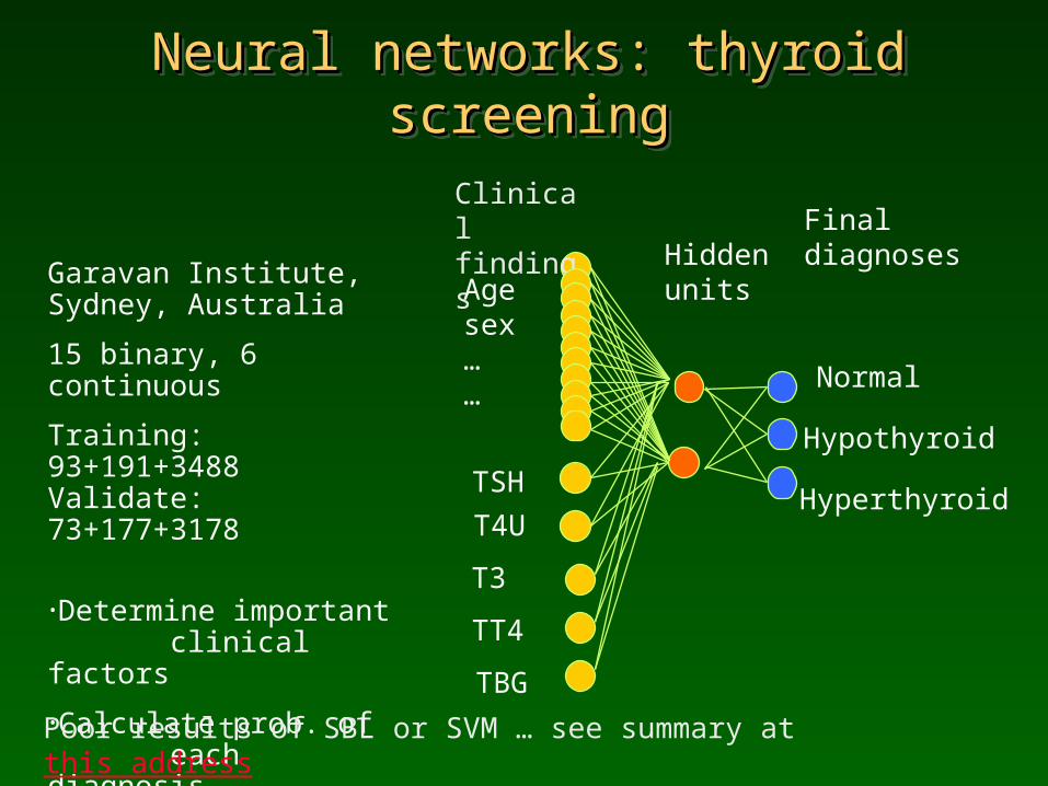
Neural networks: thyroid screeningNeural networks: thyroid screeningNeural networks: thyroid screeningNeural networks: thyroid screening

Garavan Institute, Sydney, Australia

15 binary, 6 continuous

Training: 93+191+3488 Validate: 73+177+3178

•Determine important clinical factors

•Calculate prob. of each diagnosis.

Hiddenunits

Finaldiagnoses

TSH

T4U

Clinical findings

Agesex……

T3

TT4

TBG

Normal

Hyperthyroid

Hypothyroid

Poor results of SBL or SVM … see summary at this address http://www.is.umk.pl/projects/datasets.html#Hypothyroid

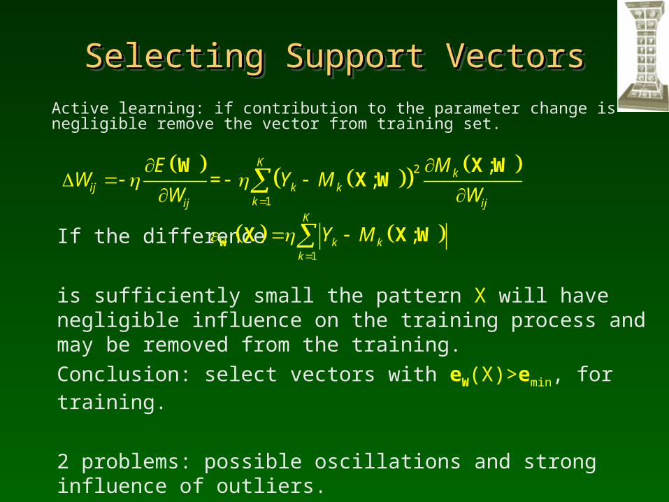
Selecting Support VectorsSelecting Support VectorsSelecting Support VectorsSelecting Support Vectors

Active learning: if contribution to the parameter change is negligible remove the vector from training set.

If the difference

is sufficiently small the pattern X will have negligible influence on the training process and may be removed from the training.Conclusion: select vectors with eW(X)>emin, for training.

2 problems: possible oscillations and strong influence of outliers. Solution: adjust emin dynamically to avoid oscillations;

remove also vectors with eW(X)>1-emin =emax

2

1

;= ;

Kk

ij k kkij ij

E MW Y M

W W

W X W

X W

1

;K

k kk

Y M

W X X W

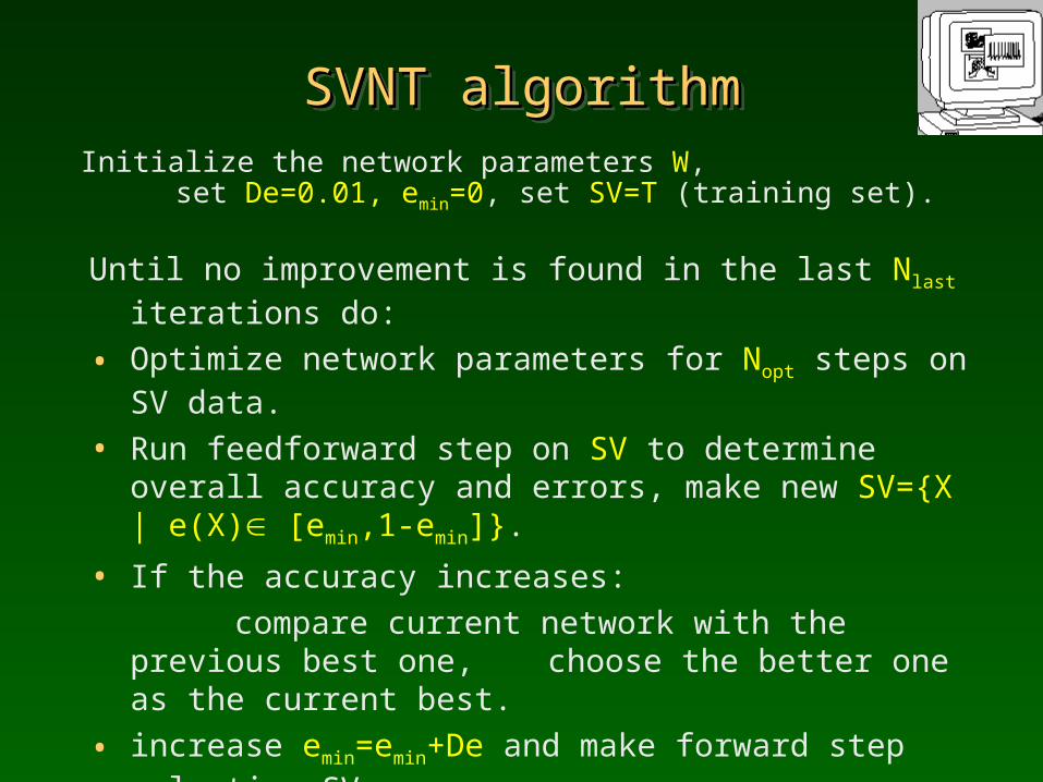
SVNT algorithmSVNT algorithmSVNT algorithmSVNT algorithmInitialize the network parameters W,

set De=0.01, emin=0, set SV=T (training set).

Until no improvement is found in the last Nlast iterations do:

• Optimize network parameters for Nopt steps on SV data.• Run feedforward step on SV to determine overall accuracy and

errors, make new SV={X | e(X) [emin,1-emin]}.• If the accuracy increases: compare current network with the previous best one,

choose the better one as the current best.• increase emin=emin+De and make forward step selecting SVs• If the number of support vectors |SV| increases:

decrease emin=emin-De;

decrease De = De/1.2 to avoid large changes

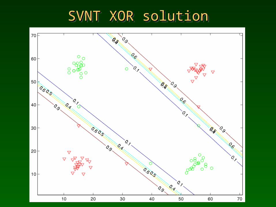
SVNT XOR solutionSVNT XOR solutionSVNT XOR solutionSVNT XOR solution

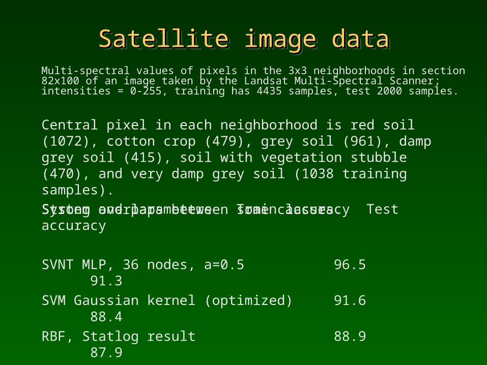
Satellite image dataSatellite image dataSatellite image dataSatellite image dataMulti-spectral values of pixels in the 3x3 neighborhoods in section 82x100 of an image taken by the Landsat Multi-Spectral Scanner; intensities = 0-255, training has 4435 samples, test 2000 samples.

Central pixel in each neighborhood is red soil (1072), cotton crop (479), grey soil (961), damp grey soil (415), soil with vegetation stubble (470), and very damp grey soil (1038 training samples). Strong overlaps between some classes.

System and parameters Train accuracy Test accuracy

SVNT MLP, 36 nodes, a=0.5 96.5 91.3SVM Gaussian kernel (optimized) 91.6 88.4 RBF, Statlog result 88.9 87.9 MLP, Statlog result 88.8 86.1 C4.5 tree 96.0 85.0

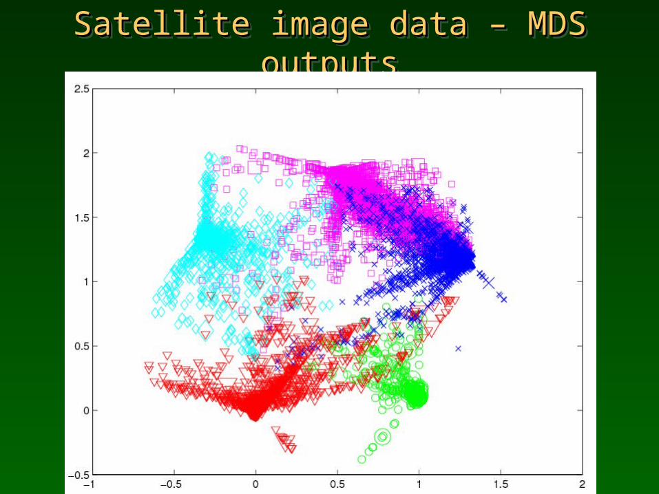
Satellite image data – MDS outputsSatellite image data – MDS outputsSatellite image data – MDS outputsSatellite image data – MDS outputs

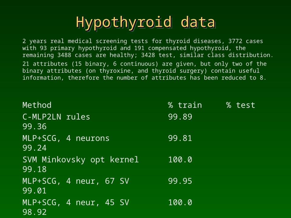
Hypothyroid dataHypothyroid dataHypothyroid dataHypothyroid data2 years real medical screening tests for thyroid diseases, 3772 cases with 93 primary hypothyroid and 191 compensated hypothyroid, the remaining 3488 cases are healthy; 3428 test, similar class distribution. 21 attributes (15 binary, 6 continuous) are given, but only two of the binary attributes (on thyroxine, and thyroid surgery) contain useful information, therefore the number of attributes has been reduced to 8.

Method % train % test C-MLP2LN rules 99.89 99.36 MLP+SCG, 4 neurons 99.81 99.24 SVM Minkovsky opt kernel 100.0 99.18 MLP+SCG, 4 neur, 67 SV 99.95 99.01 MLP+SCG, 4 neur, 45 SV 100.0 98.92 MLP+SCG, 12 neur. 100.0 98.83 Cascade correlation 100.0 98.5MLP+backprop 99.60 98.5 SVM Gaussian kernel 99.76 98.4

Hypothyroid dataHypothyroid dataHypothyroid dataHypothyroid data

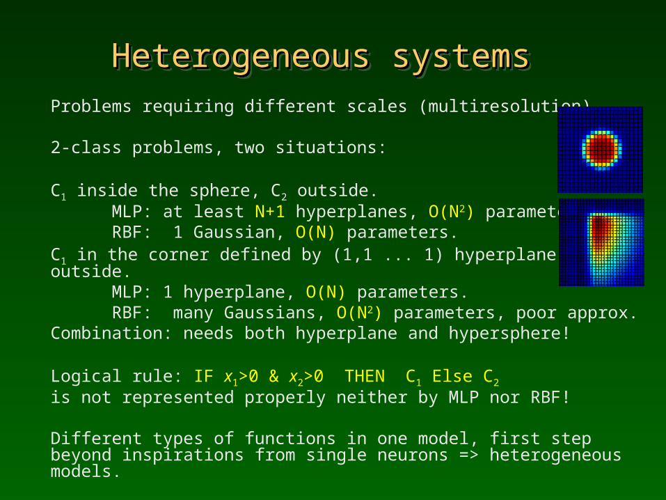
Heterogeneous systemsHeterogeneous systemsHeterogeneous systemsHeterogeneous systemsProblems requiring different scales (multiresolution).

2-class problems, two situations:

C1 inside the sphere, C2 outside.MLP: at least N+1 hyperplanes, O(N2) parameters. RBF: 1 Gaussian, O(N) parameters.

C1 in the corner defined by (1,1 ... 1) hyperplane, C2 outside.MLP: 1 hyperplane, O(N) parameters. RBF: many Gaussians, O(N2) parameters, poor approx.

Combination: needs both hyperplane and hypersphere!

Logical rule: IF x1>0 & x2>0 THEN C1 Else C2

is not represented properly neither by MLP nor RBF!

Different types of functions in one model, first step beyond inspirations from single neurons => heterogeneous models.

Heterogeneous everythingHeterogeneous everythingHeterogeneous everythingHeterogeneous everythingHomogenous systems: one type of “building blocks”, same type of decision borders, ex: neural networks, SVMs, decision trees, kNNsCommittees combine many models together, but lead to complex models that are difficult to understand.

Ockham razor: simpler systems are better. Discovering simplest class structures, inductive bias of the data, requires Heterogeneous Adaptive Systems (HAS).

HAS examples:NN with different types of neuron transfer functions.k-NN with different distance functions for each prototype.Decision Trees with different types of test criteria.

1. Start from large networks, use regularization to prune.2. Construct network adding nodes selected from a candidate pool.3. Use very flexible functions, force them to specialize.

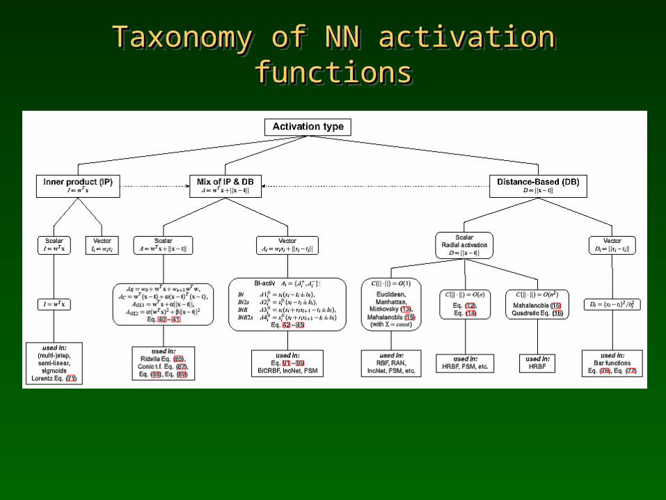
Taxonomy of NN activation functionsTaxonomy of NN activation functionsTaxonomy of NN activation functionsTaxonomy of NN activation functions

Taxonomy of NN output functionsTaxonomy of NN output functionsTaxonomy of NN output functionsTaxonomy of NN output functions

Perceptron: implements logical rule x> for x with Gaussian uncertainty.

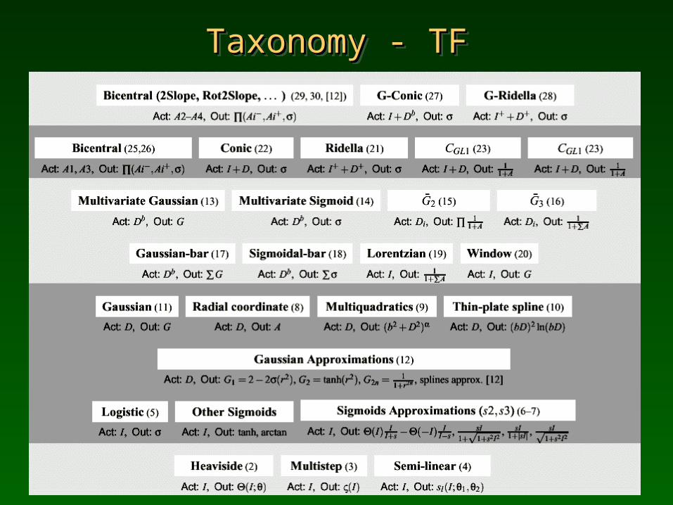
Taxonomy Taxonomy - TF- TFTaxonomy Taxonomy - TF- TF

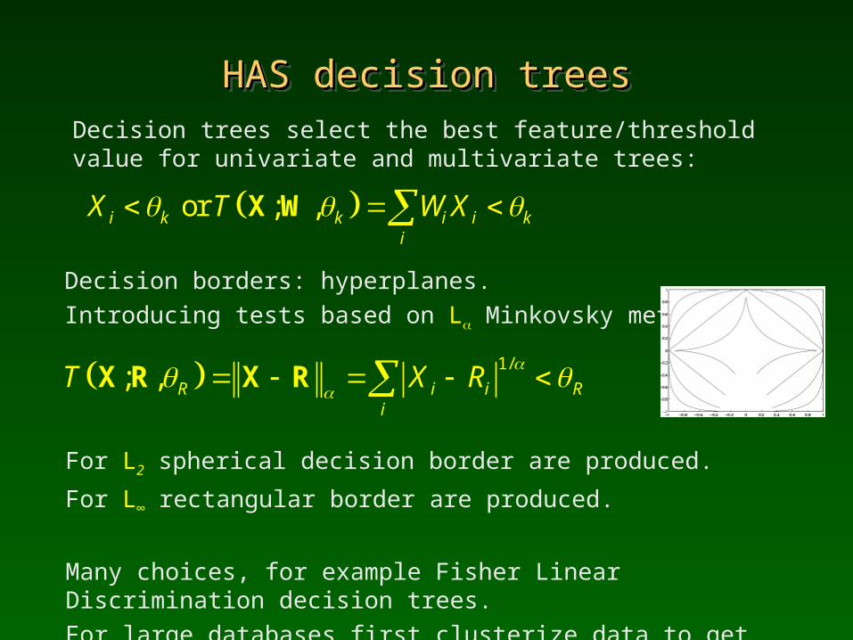
HAS decision treesHAS decision treesHAS decision treesHAS decision treesDecision trees select the best feature/threshold value for univariate and multivariate trees:

Decision borders: hyperplanes.

Introducing tests based on L Minkovsky metric.

or ; ,i k k i i ki

X T W X X W

For L2 spherical decision border are produced.

For L∞ rectangular border are produced.

Many choices, for example Fisher Linear Discrimination decision trees.

For large databases first clusterize data to get candidate references R.

1/; , R i i R

i

T X R

X R X R

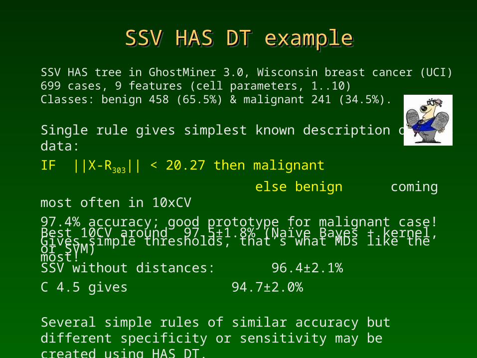
SSV HAS DT exampleSSV HAS DT exampleSSV HAS DT exampleSSV HAS DT example

SSV HAS tree in GhostMiner 3.0, Wisconsin breast cancer (UCI)699 cases, 9 features (cell parameters, 1..10)Classes: benign 458 (65.5%) & malignant 241 (34.5%).

Single rule gives simplest known description of this data: IF ||X-R303|| < 20.27 then malignant

else benign coming most often in 10xCV97.4% accuracy; good prototype for malignant case! Gives simple thresholds, that’s what MDs like the most!

Best 10CV around 97.5±1.8% (Naïve Bayes + kernel, or SVM)SSV without distances: 96.4±2.1%C 4.5 gives 94.7±2.0%

Several simple rules of similar accuracy but different specificity or sensitivity may be created using HAS DT. Need to select or weight features and select good prototypes.

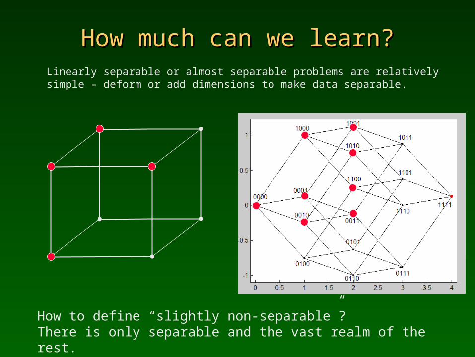
How much can we learn?How much can we learn?Linearly separable or almost separable problems are relatively simple – deform or add dimensions to make data separable.

How to define “slightly non-separable”? There is only separable and the vast realm of the rest.

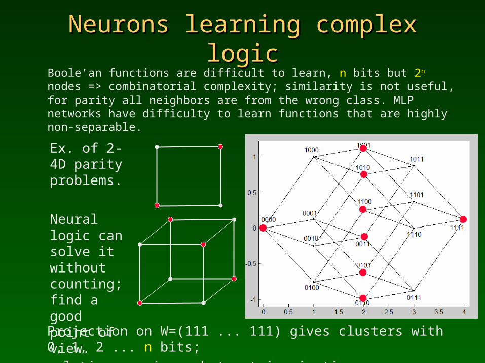
Neurons learning complex logicNeurons learning complex logicBoole’an functions are difficult to learn, n bits but 2n nodes => combinatorial complexity; similarity is not useful, for parity all neighbors are from the wrong class. MLP networks have difficulty to learn functions that are highly non-separable.

Projection on W=(111 ... 111) gives clusters with 0, 1, 2 ... n bits;solution requires abstract imagination + easy categorization.

Ex. of 2-4D parity problems.

Neural logic can solve it without counting; find a good point of view.

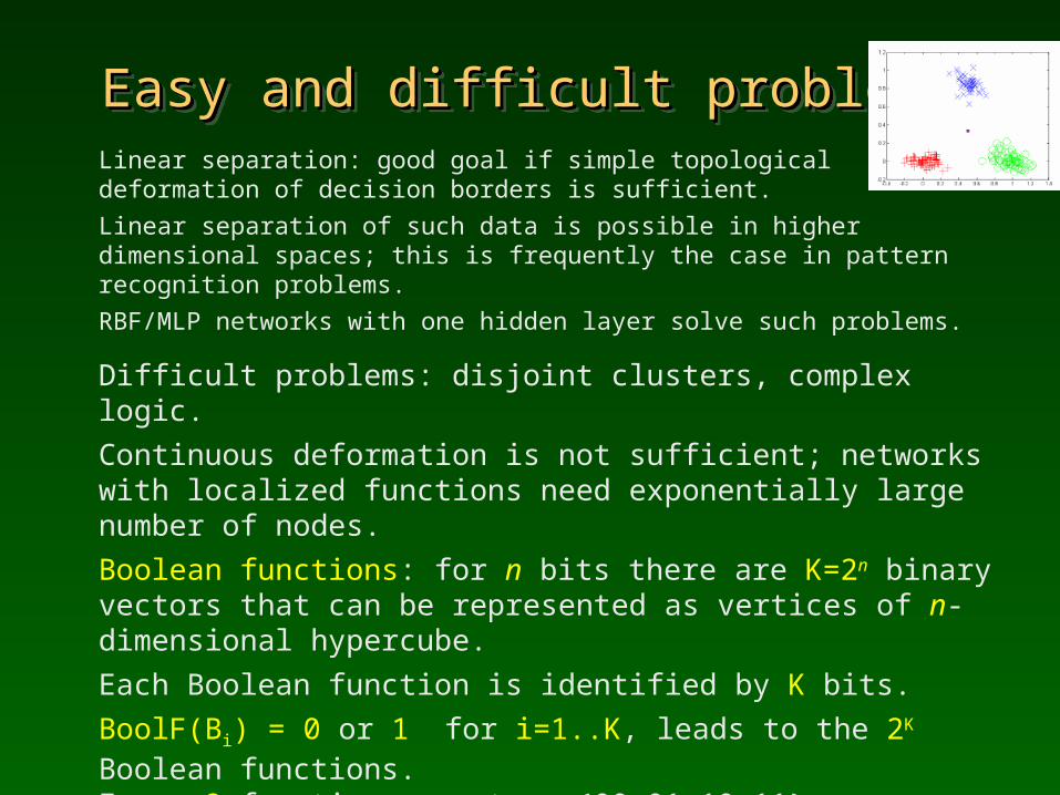
Easy and difficult problemsEasy and difficult problemsEasy and difficult problemsEasy and difficult problemsLinear separation: good goal if simple topological deformation of decision borders is sufficient.Linear separation of such data is possible in higher dimensional spaces; this is frequently the case in pattern recognition problems. RBF/MLP networks with one hidden layer solve such problems.

Difficult problems: disjoint clusters, complex logic.Continuous deformation is not sufficient; networks with localized functions need exponentially large number of nodes.Boolean functions: for n bits there are K=2n binary vectors that can be represented as vertices of n-dimensional hypercube. Each Boolean function is identified by K bits. BoolF(Bi) = 0 or 1 for i=1..K, leads to the 2K Boolean functions.Ex: n=2 functions, vectors {00,01,10,11}, Boolean functions {0000, 0001 ... 1111}, ex. 0001 = AND, 0110 = OR,each function is identified by number from 0 to 15 = 2K-1.

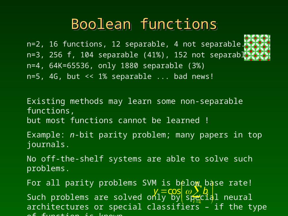
Boolean functionsBoolean functionsBoolean functionsBoolean functionsn=2, 16 functions, 12 separable, 4 not separable.n=3, 256 f, 104 separable (41%), 152 not separable.n=4, 64K=65536, only 1880 separable (3%)n=5, 4G, but << 1% separable ... bad news!

Existing methods may learn some non-separable functions, but most functions cannot be learned !

Example: n-bit parity problem; many papers in top journals.

No off-the-shelf systems are able to solve such problems.

For all parity problems SVM is below base rate!

Such problems are solved only by special neural architectures or special classifiers – if the type of function is known.

But parity is still trivial ... solved by 1

cosn

ii

y b

What NN components really do?What NN components really do?What NN components really do?What NN components really do?

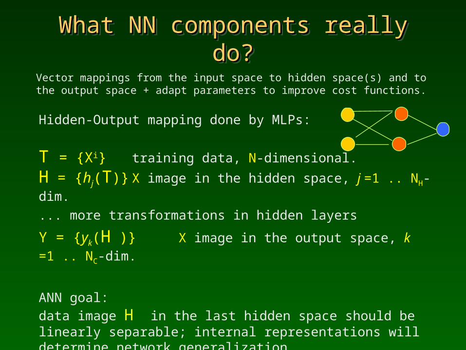
Vector mappings from the input space to hidden space(s) and to the output space + adapt parameters to improve cost functions.

Hidden-Output mapping done by MLPs:

T = {Xi} training data, N-dimensional. H = {hj(T)} X image in the hidden space, j =1 .. NH-dim.

... more transformations in hidden layers

Y = {yk(H )} X image in the output space, k =1 .. NC-dim.

ANN goal: data image H in the last hidden space should be linearly separable; internal representations will determine network generalization.

But we never look at these representations!

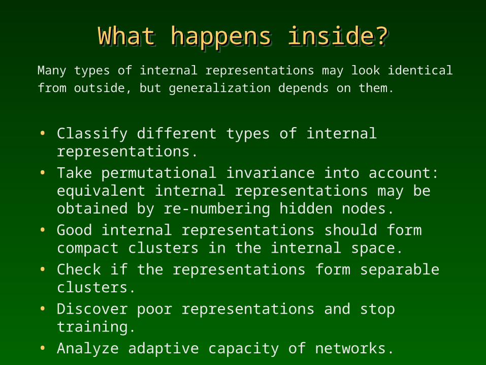
What happens inside?What happens inside?What happens inside?What happens inside?

Many types of internal representations may look identical

from outside, but generalization depends on them.

• Classify different types of internal representations.

• Take permutational invariance into account: equivalent internal representations may be obtained by re-numbering hidden nodes.

• Good internal representations should form compact clusters in the internal space.

• Check if the representations form separable clusters.

• Discover poor representations and stop training.

• Analyze adaptive capacity of networks.

• .....

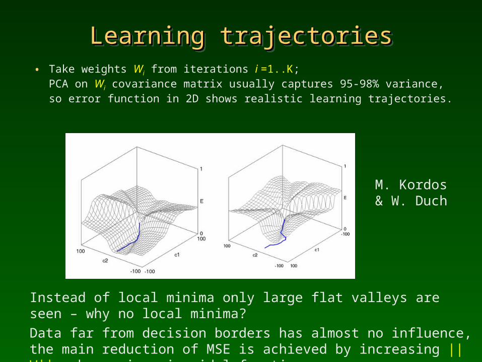
Learning trajectoriesLearning trajectoriesLearning trajectoriesLearning trajectories• Take weights Wi from iterations i =1..K;

PCA on Wi covariance matrix usually captures 95-98% variance, so error function in 2D shows realistic learning trajectories.

Instead of local minima only large flat valleys are seen – why no local minima? Data far from decision borders has almost no influence, the main reduction of MSE is achieved by increasing ||W||, sharpening sigmoidal functions.

M. Kordos & W. Duch

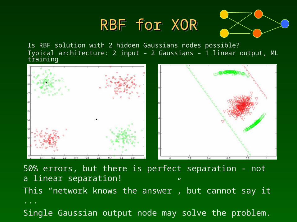
RBF for XORRBF for XORRBF for XORRBF for XORIs RBF solution with 2 hidden Gaussians nodes possible?Typical architecture: 2 input – 2 Gaussians – 1 linear output, ML training

50% errors, but there is perfect separation - not a linear separation! This “network knows the answer”, but cannot say it ... Single Gaussian output node may solve the problem. Output weights provide reference hyperplanes (red and green lines), not the separating hyperplanes like in case of MLP.

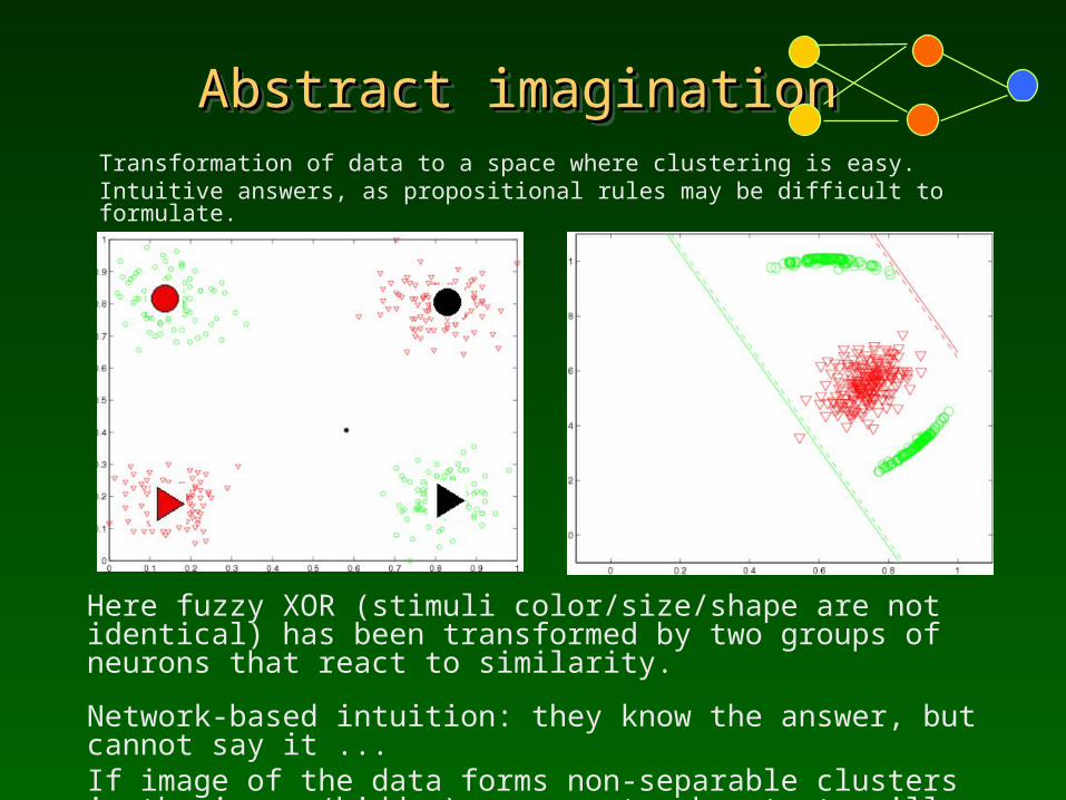
Abstract imagination Abstract imagination Abstract imagination Abstract imagination Transformation of data to a space where clustering is easy.Intuitive answers, as propositional rules may be difficult to formulate.

Here fuzzy XOR (stimuli color/size/shape are not identical) has been transformed by two groups of neurons that react to similarity.

Network-based intuition: they know the answer, but cannot say it ... If image of the data forms non-separable clusters in the inner (hidden) space network outputs will be often wrong.

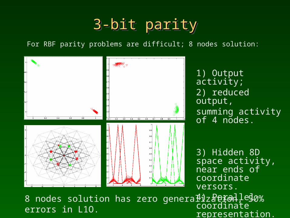
3-bit parity3-bit parity3-bit parity3-bit parityFor RBF parity problems are difficult; 8 nodes solution:

1) Output activity;2) reduced output,summing activity of 4 nodes.

3) Hidden 8D space activity, near ends of coordinate versors. 4) Parallel coordinate representation.

8 nodes solution has zero generalization, 50% errors in L1O.

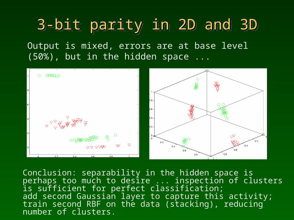
3-bit parity in 2D and 3D3-bit parity in 2D and 3D3-bit parity in 2D and 3D3-bit parity in 2D and 3DOutput is mixed, errors are at base level (50%), but in the hidden space ...

Conclusion: separability in the hidden space is perhaps too much to desire ... inspection of clusters is sufficient for perfect classification; add second Gaussian layer to capture this activity; train second RBF on the data (stacking), reducing number of clusters.

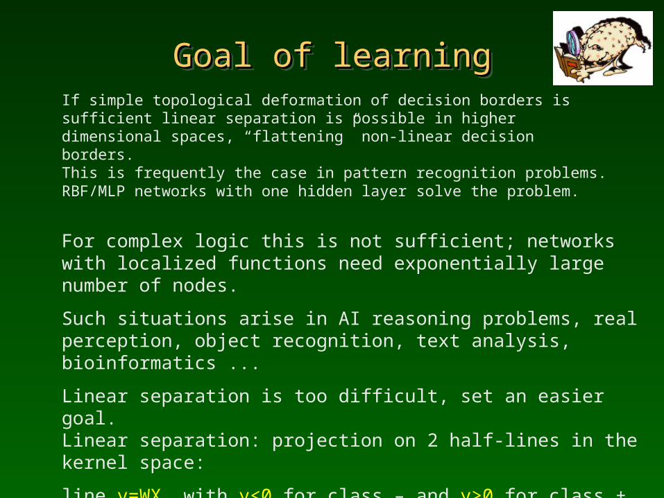
Goal of learningGoal of learningGoal of learningGoal of learningIf simple topological deformation of decision borders is sufficient linear separation is possible in higher dimensional spaces, “flattening” non-linear decision borders. This is frequently the case in pattern recognition problems. RBF/MLP networks with one hidden layer solve the problem.

For complex logic this is not sufficient; networks with localized functions need exponentially large number of nodes.

Such situations arise in AI reasoning problems, real perception, object recognition, text analysis, bioinformatics ...

Linear separation is too difficult, set an easier goal. Linear separation: projection on 2 half-lines in the kernel space:

line y=WX, with y<0 for class – and y>0 for class +.

Simplest extension: separation into k-intervals, or k-separability.

For parity: find direction W with minimum # of intervals, y=W.X

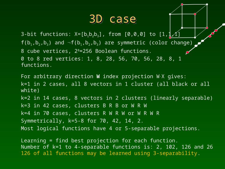
3D case3D case3D case3D case3-bit functions: X=[b1b2b3], from [0,0,0] to [1,1,1]

f(b1,b2,b3) and f(b1,b2,b3) are symmetric (color change)

8 cube vertices, 28=256 Boolean functions. 0 to 8 red vertices: 1, 8, 28, 56, 70, 56, 28, 8, 1 functions.

For arbitrary direction W index projection W.X gives: k=1 in 2 cases, all 8 vectors in 1 cluster (all black or all white)k=2 in 14 cases, 8 vectors in 2 clusters (linearly separable) k=3 in 42 cases, clusters B R B or W R Wk=4 in 70 cases, clusters R W R W or W R W RSymmetrically, k=5-8 for 70, 42, 14, 2. Most logical functions have 4 or 5-separable projections.

Learning = find best projection for each function. Number of k=1 to 4-separable functions is: 2, 102, 126 and 26126 of all functions may be learned using 3-separability.

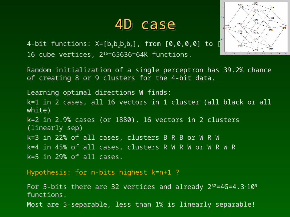
4D case4D case4D case4D case4-bit functions: X=[b1b2b3b4], from [0,0,0,0] to [1,1,1,1]

16 cube vertices, 216=65636=64K functions.

Random initialization of a single perceptron has 39.2% chance of creating 8 or 9 clusters for the 4-bit data.

Learning optimal directions W finds: k=1 in 2 cases, all 16 vectors in 1 cluster (all black or all white)k=2 in 2.9% cases (or 1880), 16 vectors in 2 clusters (linearly sep) k=3 in 22% of all cases, clusters B R B or W R Wk=4 in 45% of all cases, clusters R W R W or W R W Rk=5 in 29% of all cases.

Hypothesis: for n-bits highest k=n+1 ?

For 5-bits there are 32 vertices and already 232=4G=4.3.109 functions.Most are 5-separable, less than 1% is linearly separable!

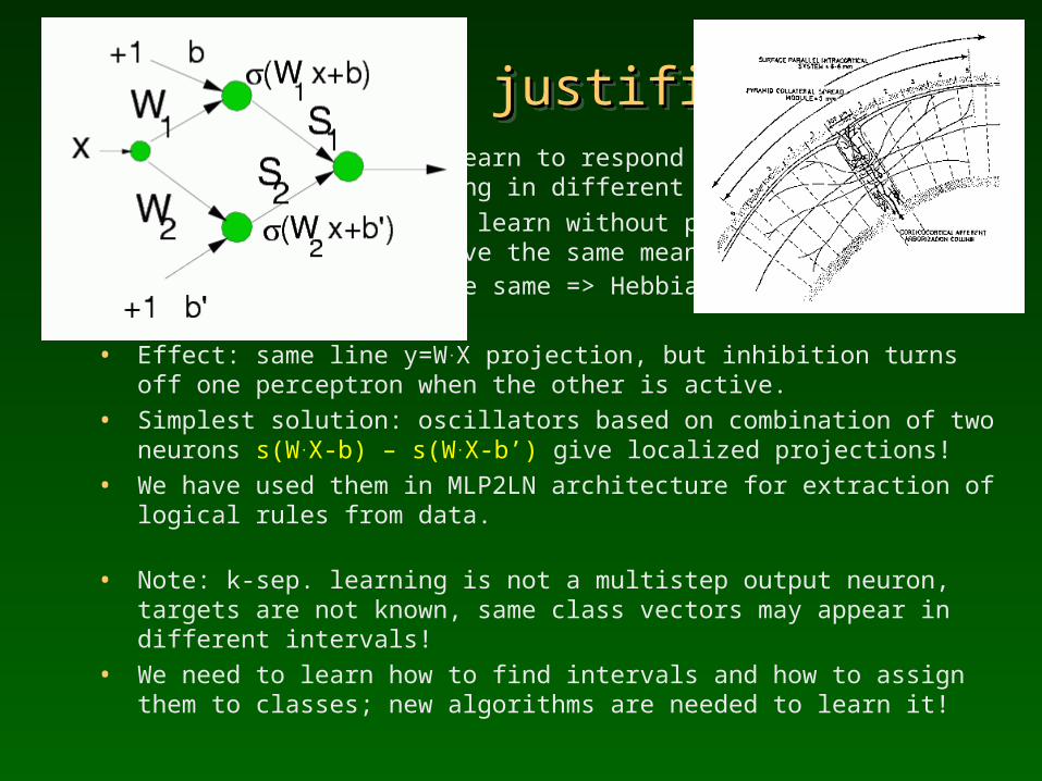
Biological justificationBiological justificationBiological justificationBiological justification• Cortical columns may learn to respond to stimuli with complex logic

resonating in different way.• The second column will learn without problems that such different

reactions have the same meaning: inputs xi and training targets yj. are same => Hebbian learning DWij ~ xi yj => identical weights.

• Effect: same line y=W.X projection, but inhibition turns off one perceptron when the other is active.

• Simplest solution: oscillators based on combination of two neurons s(W.X-b) – s(W.X-b’) give localized projections!

• We have used them in MLP2LN architecture for extraction of logical rules from data.

• Note: k-sep. learning is not a multistep output neuron, targets are not known, same class vectors may appear in different intervals!

• We need to learn how to find intervals and how to assign them to classes; new algorithms are needed to learn it!

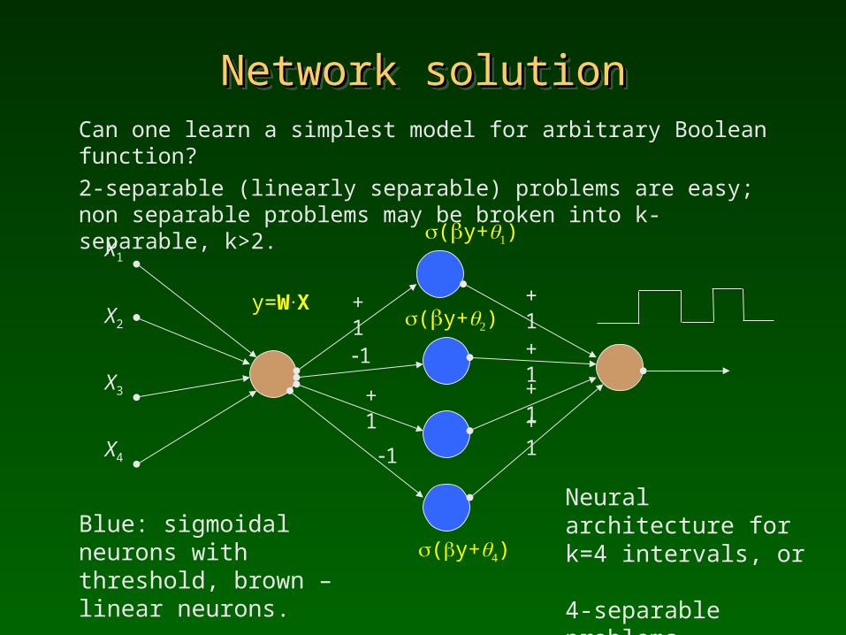
Network solutionNetwork solutionNetwork solutionNetwork solutionCan one learn a simplest model for arbitrary Boolean function? 2-separable (linearly separable) problems are easy; non separable problems may be broken into k-separable, k>2.

Blue: sigmoidal neurons with threshold, brown – linear neurons.

X1

X2

X3

X4

y=W.

X

+1

1

+11

(y+)

(y+)

+1

+1+1+1

(y+)

Neural architecture for k=4 intervals, or 4-separable problems.

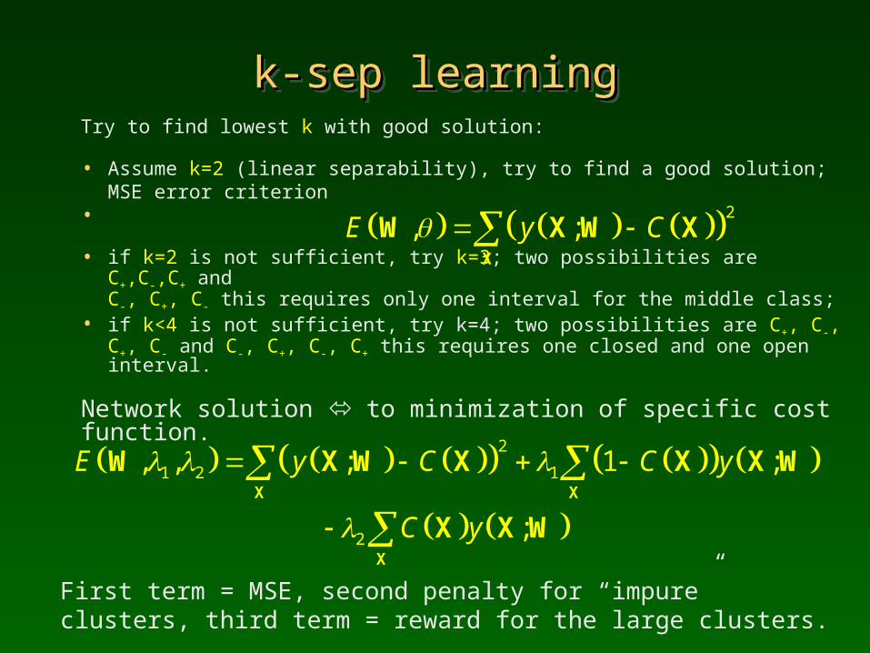
k-sep learningk-sep learningk-sep learningk-sep learningTry to find lowest k with good solution:

• Assume k=2 (linear separability), try to find a good solution;

MSE error criterion•

• if k=2 is not sufficient, try k=3; two possibilities are C+,C-,C+ and C-, C+, C- this requires only one interval for the middle class;

• if k<4 is not sufficient, try k=4; two possibilities are C+, C-, C+, C- and C-, C+, C-, C+ this requires one closed and one open interval.

Network solution to minimization of specific cost function.

2

1 2 1

2

, , ; 1 ;

;

E y C C y

C y

X X

X

W X W X X X W

X X W

First term = MSE, second penalty for “impure” clusters, third term = reward for the large clusters.

2, ;E y C

X

W X W X

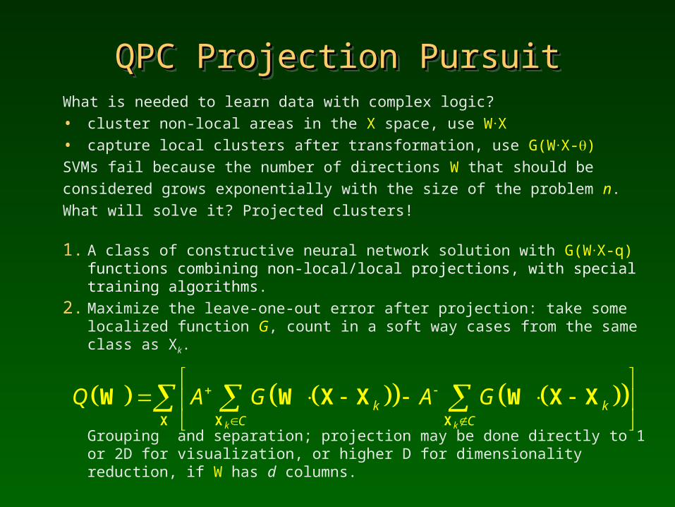
QPC Projection PursuitQPC Projection PursuitQPC Projection PursuitQPC Projection PursuitWhat is needed to learn data with complex logic?• cluster non-local areas in the X space, use W.X• capture local clusters after transformation, use G(W.X-) SVMs fail because the number of directions W that should be considered grows exponentially with the size of the problem n.What will solve it? Projected clusters!

1. A class of constructive neural network solution with G(W.X-q) functions combining non-local/local projections, with special training algorithms.

2. Maximize the leave-one-out error after projection: take some localized function G, count in a soft way cases from the same class as Xk.

Grouping and separation; projection may be done directly to 1 or 2D for visualization, or higher D for dimensionality reduction, if W has d columns.

k k

k kC C

Q A G A G

X X X

W W X X W X X

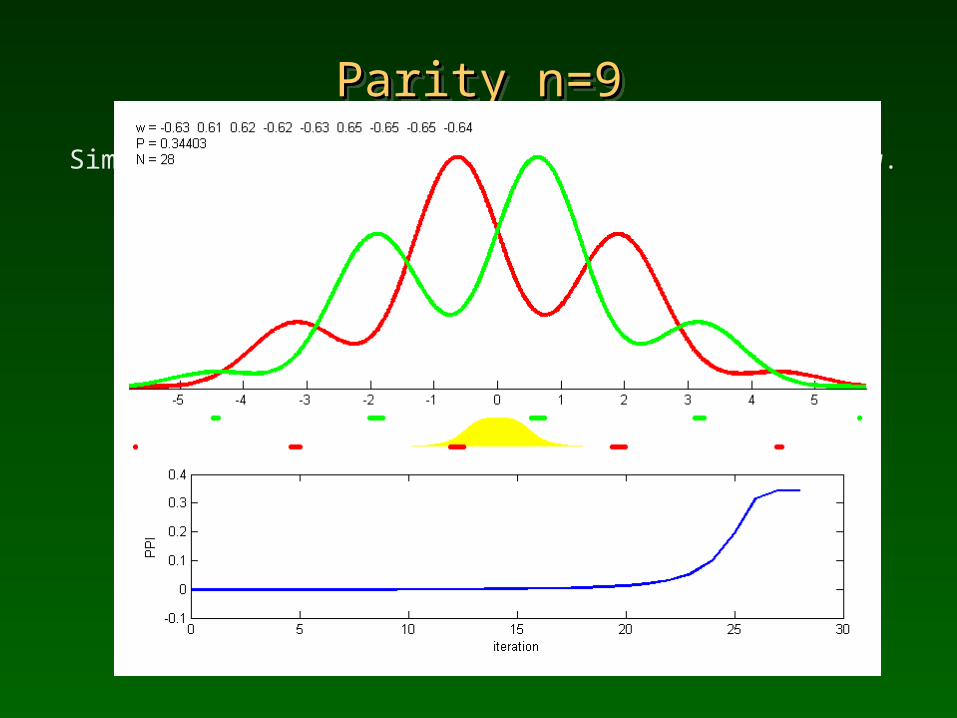
Parity n=9Parity n=9Parity n=9Parity n=9

Simple gradient learning; quality index shown below.

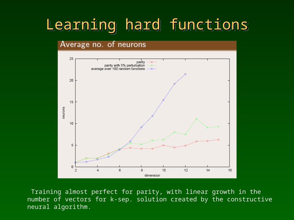
Learning hard functionsLearning hard functionsLearning hard functionsLearning hard functions

Training almost perfect for parity, with linear growth in the number of vectors for k-sep. solution created by the constructive neural algorithm.

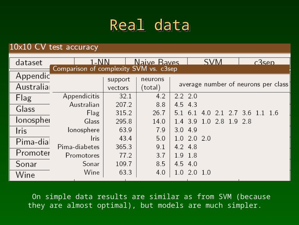
Real dataReal dataReal dataReal data

On simple data results are similar as from SVM (because they are almost optimal), but models are much simpler.

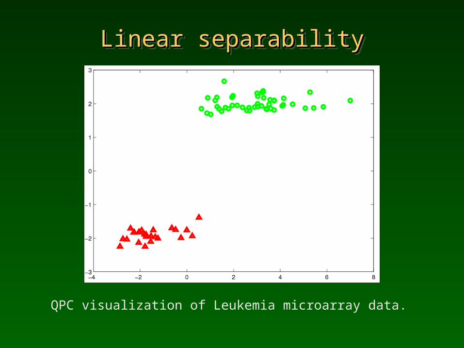
Linear separabilityLinear separabilityLinear separabilityLinear separability

QPC visualization of Leukemia microarray data.

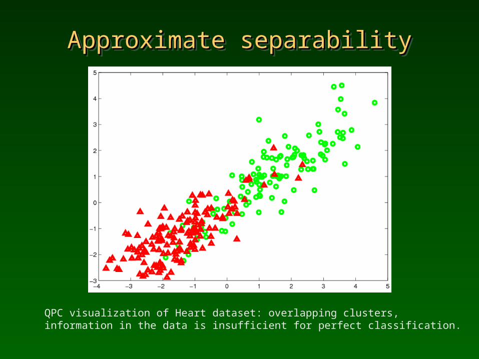
Approximate separabilityApproximate separabilityApproximate separabilityApproximate separability

QPC visualization of Heart dataset: overlapping clusters, information in the data is insufficient for perfect classification.

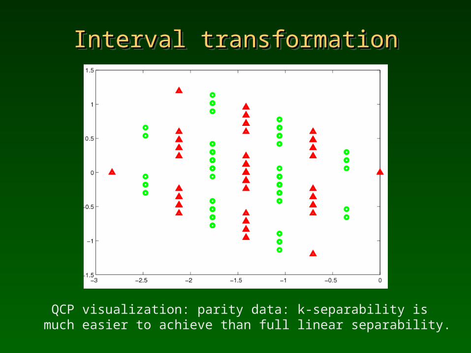
Interval transformationInterval transformationInterval transformationInterval transformation

QCP visualization: parity data: k-separability is much easier to achieve than full linear separability.

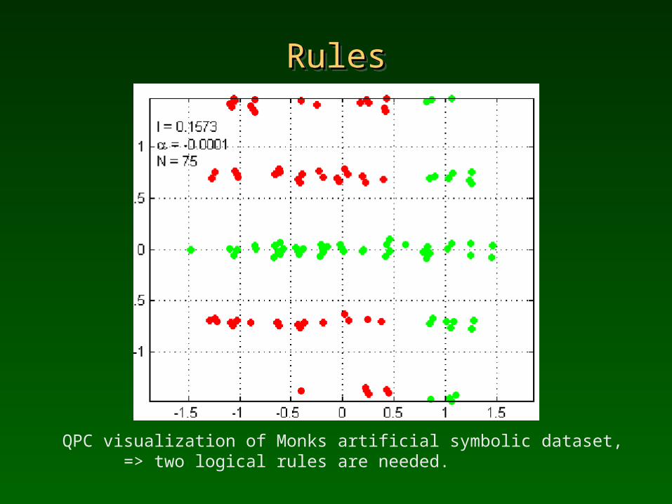
RulesRulesRulesRules

QPC visualization of Monks artificial symbolic dataset, => two logical rules are needed.

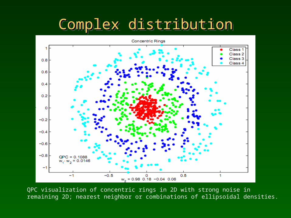
Complex distributionComplex distributionComplex distributionComplex distribution

QPC visualization of concentric rings in 2D with strong noise in remaining 2D; nearest neighbor or combinations of ellipsoidal densities.

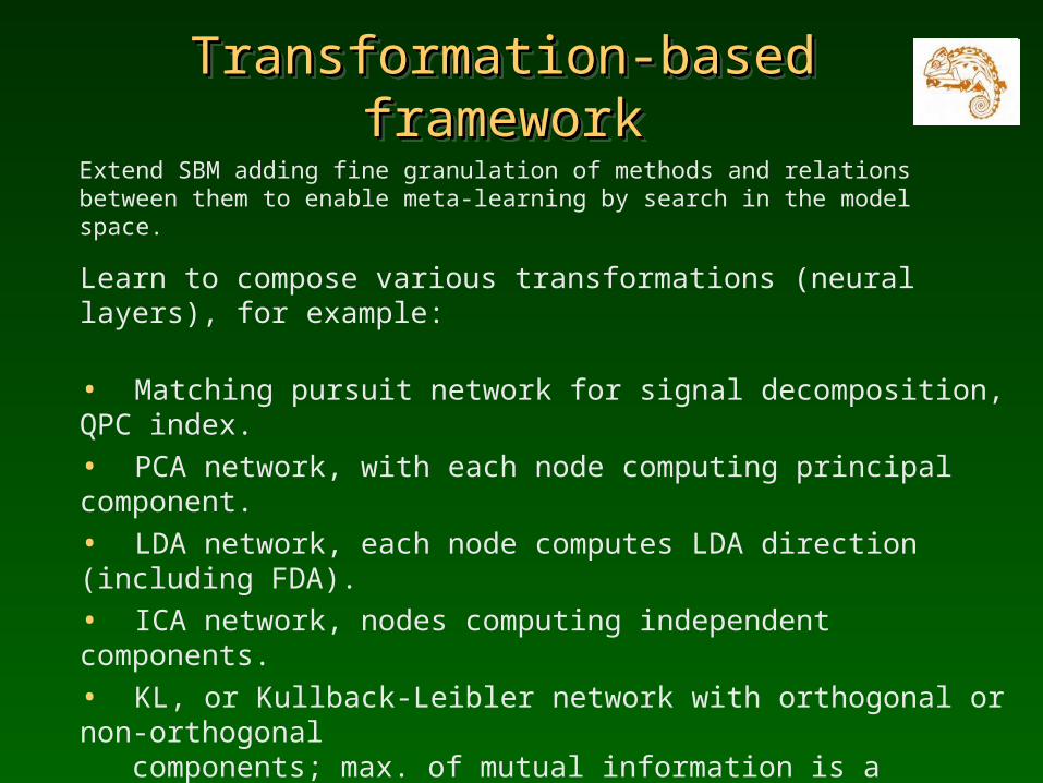
Transformation-based frameworkTransformation-based frameworkTransformation-based frameworkTransformation-based framework

Extend SBM adding fine granulation of methods and relations between them to enable meta-learning by search in the model space.

Learn to compose various transformations (neural layers), for example:

• Matching pursuit network for signal decomposition, QPC index.• PCA network, with each node computing principal component.• LDA network, each node computes LDA direction (including FDA).• ICA network, nodes computing independent components.• KL, or Kullback-Leibler network with orthogonal or non-orthogonal components; max. of mutual information is a special case • 2 and other statistical tests for dependency to aggregate features.• Factor analysis network, computing common and unique factors.• Matching pursuit network for signal decomposition.Evolving Transformation Systems (Goldfarb 1990-2009), unified paradigm for inductive learning and structural representations.

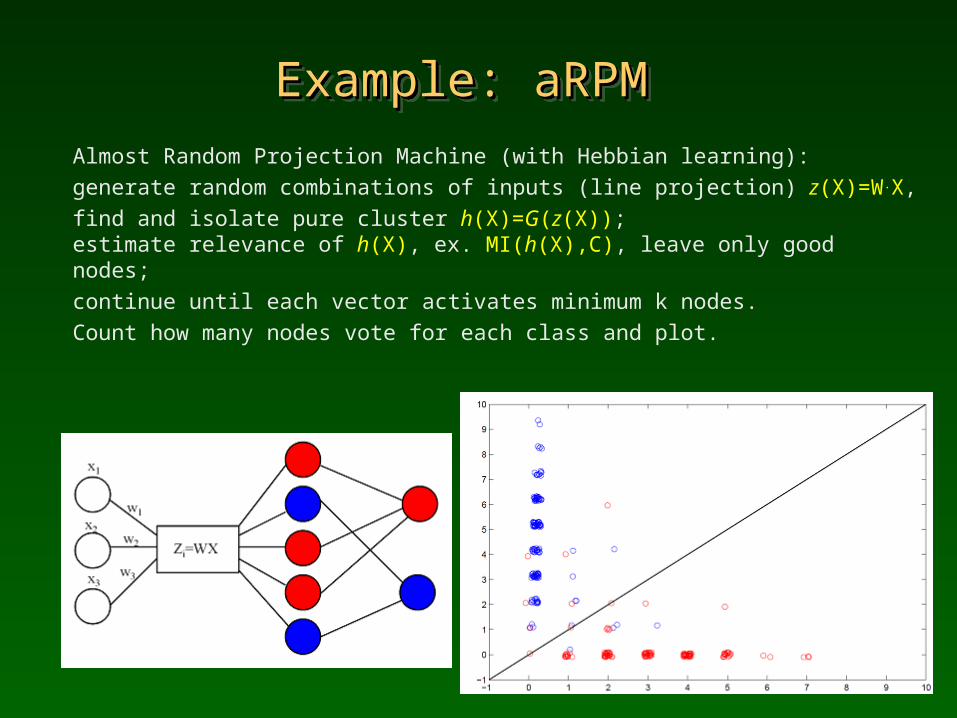
Example: aRPMExample: aRPMExample: aRPMExample: aRPM

Almost Random Projection Machine (with Hebbian learning): generate random combinations of inputs (line projection) z(X)=W.X, find and isolate pure cluster h(X)=G(z(X)); estimate relevance of h(X), ex. MI(h(X),C), leave only good nodes;continue until each vector activates minimum k nodes.Count how many nodes vote for each class and plot.

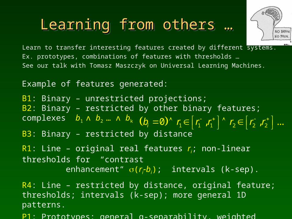
Learning from others … Learning from others … Learning from others … Learning from others …

Learn to transfer interesting features created by different systems.Ex. prototypes, combinations of features with thresholds … See our talk with Tomasz Maszczyk on Universal Learning Machines.Example of features generated:

B1: Binary – unrestricted projections; B2: Binary – restricted by other binary features; complexes b1 ᴧ b2 … ᴧ bk

B3: Binary – restricted by distance

R1: Line – original real features ri; non-linear thresholds for “contrast enhancement“ (ribi); intervals (k-sep).

R4: Line – restricted by distance, original feature; thresholds; intervals (k-sep); more general 1D patterns. P1: Prototypes: general q-separability, weighted distance functions or specialized kernels. M1: Motifs, based on correlations between elements rather than input values.

1 1 1 2 2 20 , , ...ib r r r r r r

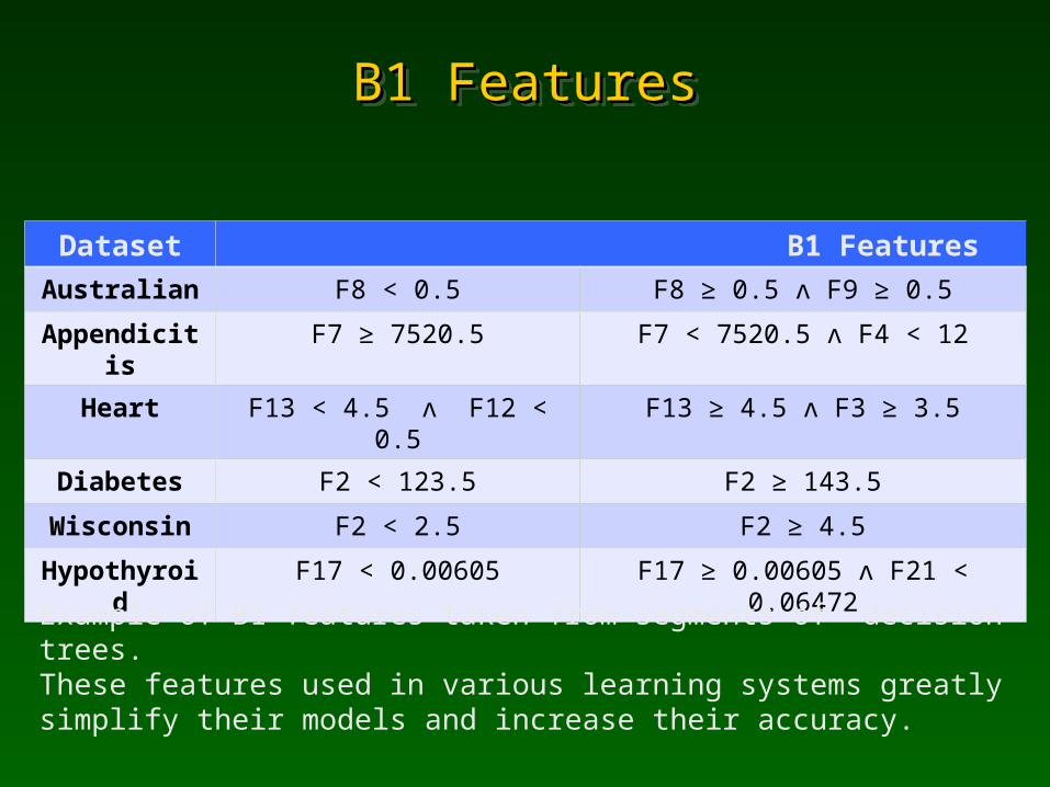
B1 FeaturesB1 FeaturesB1 FeaturesB1 Features

Dataset B1 Features

Australian F8 < 0.5 F8 ≥ 0.5 ᴧ F9 ≥ 0.5

Appendicitis F7 ≥ 7520.5 F7 < 7520.5 ᴧ F4 < 12

Heart F13 < 4.5 ᴧ F12 < 0.5 F13 ≥ 4.5 ᴧ F3 ≥ 3.5

Diabetes F2 < 123.5 F2 ≥ 143.5

Wisconsin F2 < 2.5 F2 ≥ 4.5

Hypothyroid F17 < 0.00605 F17 ≥ 0.00605 ᴧ F21 < 0.06472

Example of B1 features taken from segments of decision trees.These features used in various learning systems greatly simplify their models and increase their accuracy.

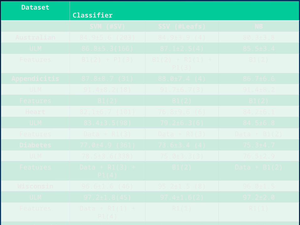
Dataset Classifier

SVM (#SV) SSV (#Leafs) NB

Australian 84.9±5.6 (203) 84.9±3.9 (4) 80.3±3.8

ULM 86.8±5.3(166) 87.1±2.5(4) 85.5±3.4

Features B1(2) + P1(3) B1(2) + R1(1) + P1(3) B1(2)

Appendicitis 87.8±8.7 (31) 88.0±7.4 (4) 86.7±6.6

ULM 91.4±8.2(18) 91.7±6.7(3) 91.4±8.2

Features B1(2) B1(2) B1(2)

Heart 82.1±6.7 (101) 76.8±9.6 (6) 84.2±6.1

ULM 83.4±3.5(98) 79.2±6.3(6) 84.5±6.8

Features Data + R1(3) Data + R1(3) Data + B1(2)

Diabetes 77.0±4.9 (361) 73.6±3.4 (4) 75.3±4.7

ULM 78.5±3.6(338) 75.0±3.3(3) 76.5±2.9

Features Data + R1(3) + P1(4) B1(2) Data + B1(2)

Wisconsin 96.6±1.6 (46) 95.2±1.5 (8) 96.0±1.5

ULM 97.2±1.8(45) 97.4±1.6(2) 97.2±2.0

Features Data + R1(1) + P1(4) R1(1) R1(1)

Hypothyroid 94.1±0.6 (918) 99.7±0.5 (12) 41.3±8.3

ULM 99.5±0.4(80) 99.6±0.4(8) 98.1±0.7

Features Data + B1(2) Data + B1(2) Data + B1(2)

Meta-learningMeta-learningMeta-learningMeta-learning

Meta-learning means different things for different people.Some will call “meta” any learning of many models (ex. Weka), ranking them, arcing, boosting, bagging, or creating an ensemble in many ways optimization of parameters to integrate models.Stacking: learn new models on errors of the previous ones.

Landmarking: characterize many datasets and remember which method worked the best on each dataset.Compare new dataset to the reference ones; define various measures (not easy) and use similarity-based methods. Regression models created for each algorithm on parameters that describe data to predict their expected accuracy.Goal: rank potentially useful algorithms.

Rather limited success …

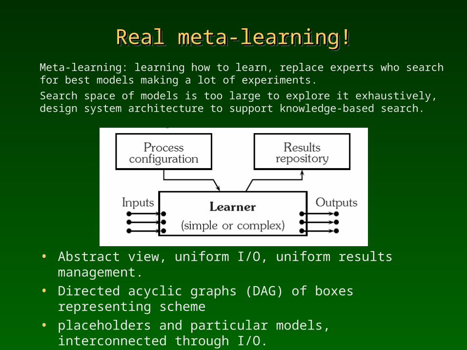
Real meta-learning!Real meta-learning!Real meta-learning!Real meta-learning!

Meta-learning: learning how to learn, replace experts who search for best models making a lot of experiments.Search space of models is too large to explore it exhaustively, design system architecture to support knowledge-based search.

• Abstract view, uniform I/O, uniform results management.• Directed acyclic graphs (DAG) of boxes representing scheme• placeholders and particular models, interconnected through I/O.• Configuration level for meta-schemes, expanded at runtime level.An exercise in software engineering for data mining!

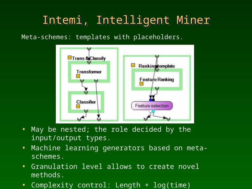
Intemi, Intelligent MinerIntemi, Intelligent MinerIntemi, Intelligent MinerIntemi, Intelligent MinerMeta-schemes: templates with placeholders.

• May be nested; the role decided by the input/output types.• Machine learning generators based on meta-schemes.• Granulation level allows to create novel methods.• Complexity control: Length + log(time)• A unified meta-parameters description, defining the range of sensible

values and the type of the parameter changes.

Advanced meta-learningAdvanced meta-learningAdvanced meta-learningAdvanced meta-learning• Extracting meta-rules, describing interesting search directions.• Finding the correlations occurring among different items in

most accurate results, identifying different machine (algorithmic) structures with similar behavior in an area of the model space.

• Depositing the knowledge they gain in a reusable meta-knowledge repository (for meta-learning experience exchange between different meta-learners).

• A uniform representation of the meta-knowledge, extending expert knowledge, adjusting the prior knowledge according to performed tests.

• Finding new successful complex structures and converting them into meta-schemes (which we call meta abstraction) by replacing proper substructures by placeholders.

• Beyond transformations & feature spaces: actively search for info.

Intemi software (N. Jankowski and K. Grąbczewski) incorporating these ideas and more is coming “soon” ...

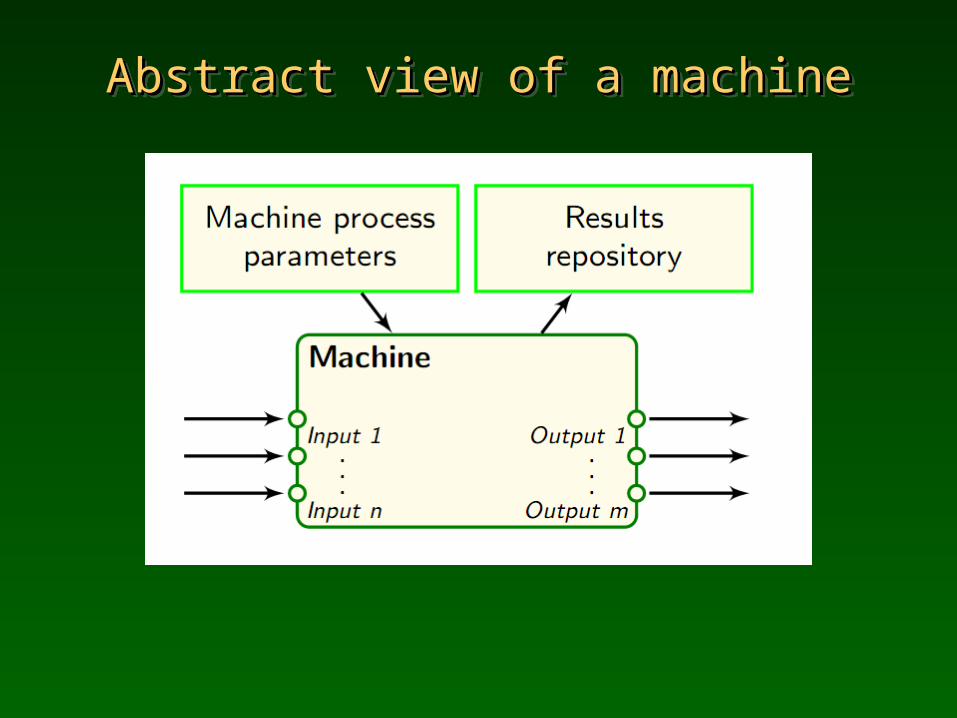
Abstract view of a machineAbstract view of a machineAbstract view of a machineAbstract view of a machine

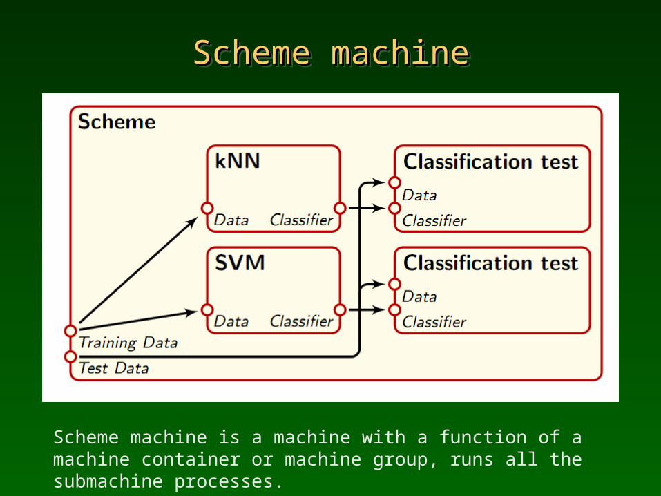
Scheme machineScheme machineScheme machineScheme machine

Scheme machine is a machine with a function of a machine container or machine group, runs all the submachine processes.

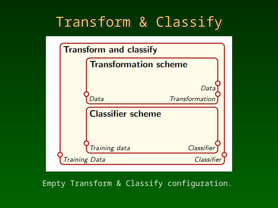
Transform & ClassifyTransform & ClassifyTransform & ClassifyTransform & Classify

Empty Transform & Classify configuration.

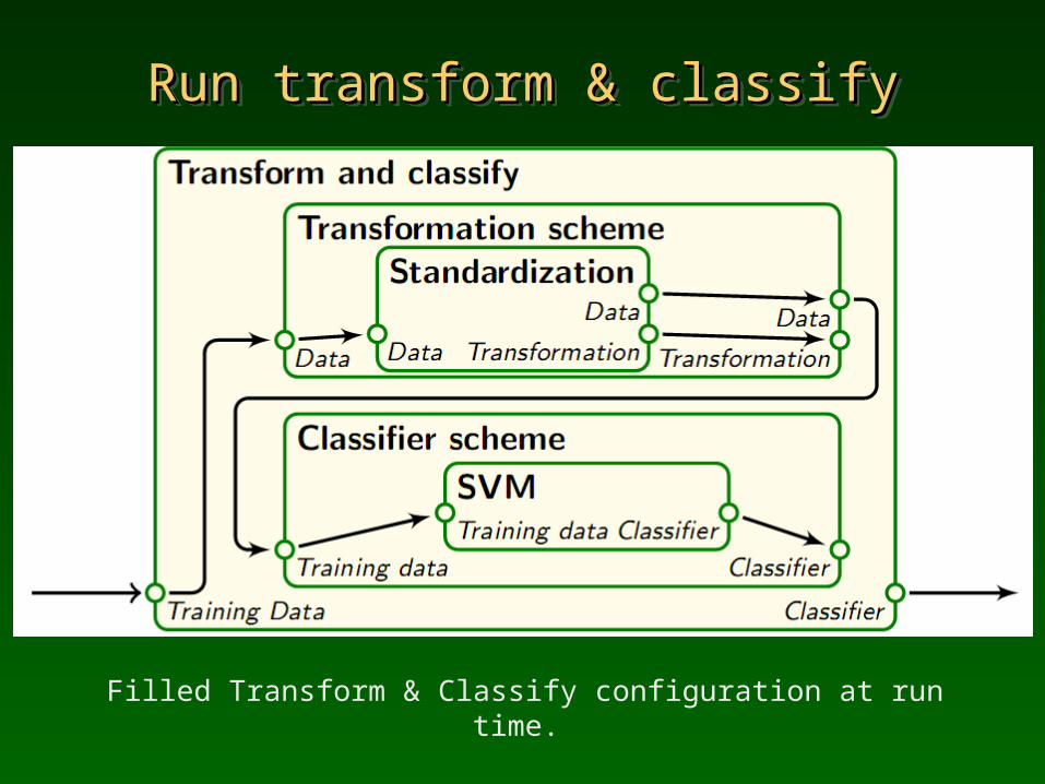
Run transform & classifyRun transform & classifyRun transform & classifyRun transform & classify

Filled Transform & Classify configuration at run time.

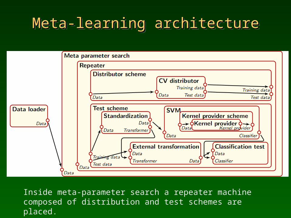
Meta-learning architectureMeta-learning architectureMeta-learning architectureMeta-learning architecture

Inside meta-parameter search a repeater machine composed of distribution and test schemes are placed.

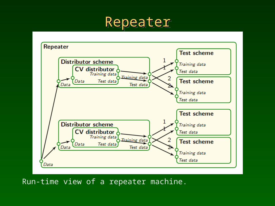
RepeaterRepeaterRepeaterRepeater

Run-time view of a repeater machine.

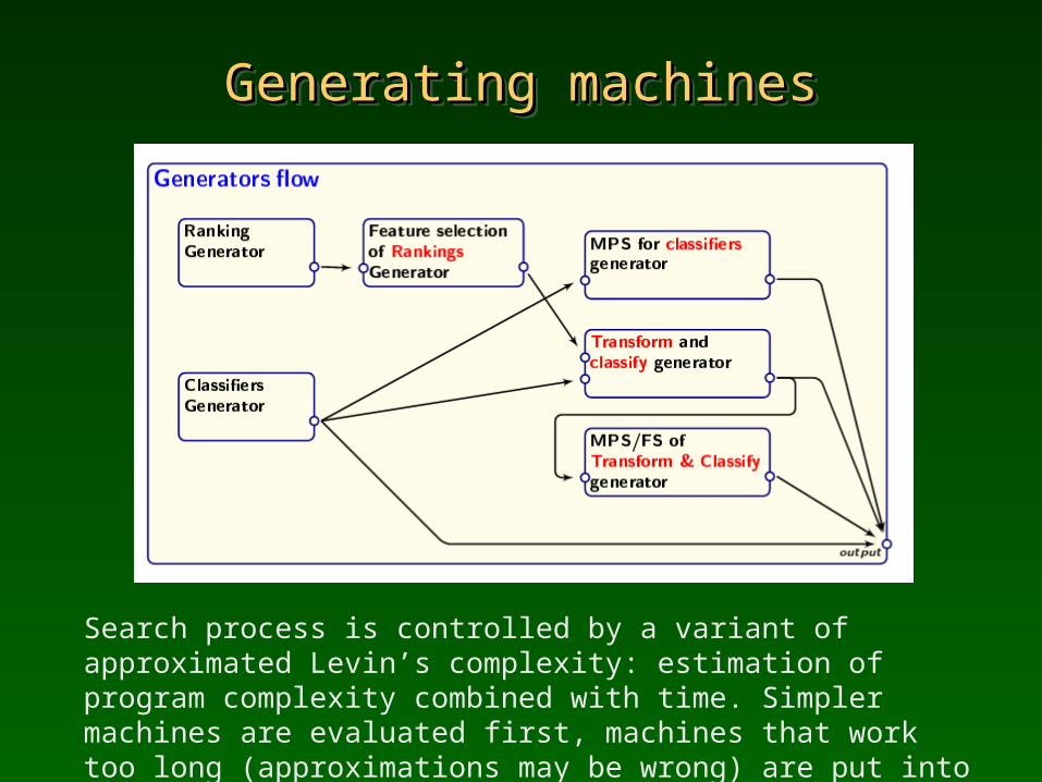
Generating machinesGenerating machinesGenerating machinesGenerating machines

Search process is controlled by a variant of approximated Levin’s complexity: estimation of program complexity combined with time. Simpler machines are evaluated first, machines that work too long (approximations may be wrong) are put into quarantine.

Pre-compute what you canPre-compute what you canPre-compute what you canPre-compute what you can

and use “machine unification” to get substantial savings!

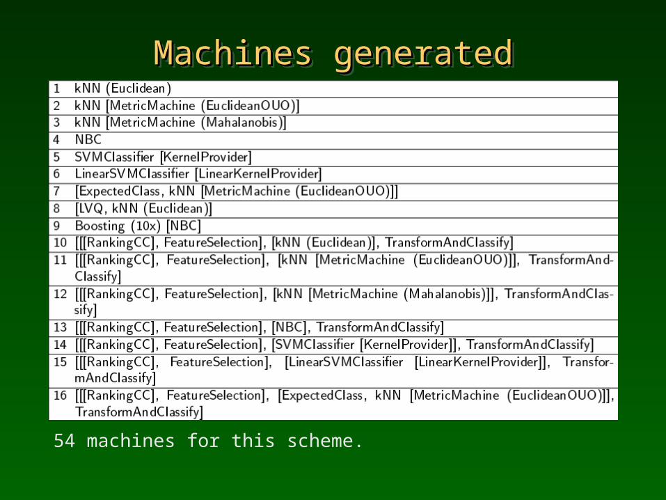
Machines generatedMachines generatedMachines generatedMachines generated

54 machines for this scheme.

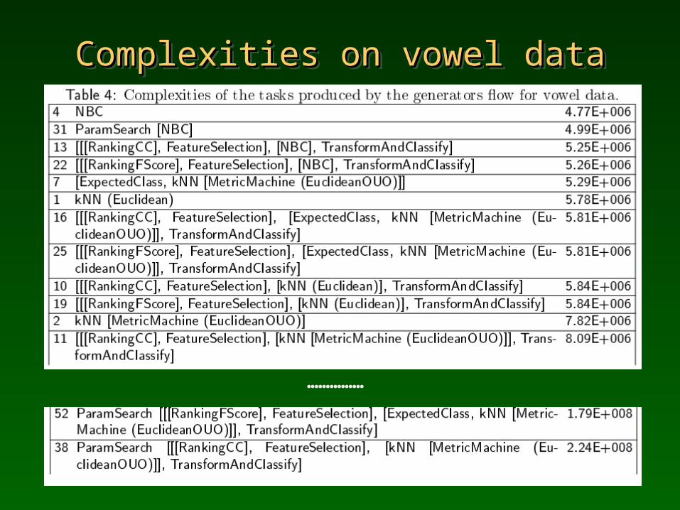
Complexities on vowel dataComplexities on vowel dataComplexities on vowel dataComplexities on vowel data

……………

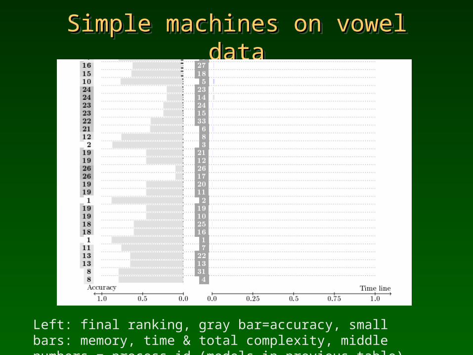
Simple machines on vowel dataSimple machines on vowel dataSimple machines on vowel dataSimple machines on vowel data

Left: final ranking, gray bar=accuracy, small bars: memory, time & total complexity, middle numbers = process id (models in previous table).

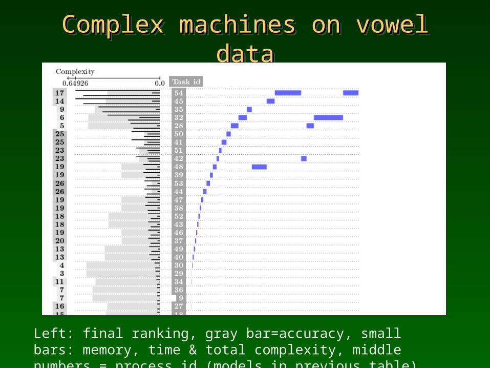
Complex machines on vowel dataComplex machines on vowel dataComplex machines on vowel dataComplex machines on vowel data

Left: final ranking, gray bar=accuracy, small bars: memory, time & total complexity, middle numbers = process id (models in previous table).

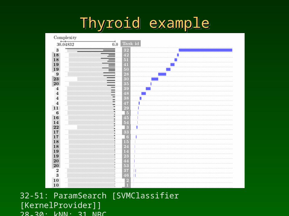
Thyroid exampleThyroid exampleThyroid exampleThyroid example

32-51: ParamSearch [SVMClassifier [KernelProvider]]28-30: kNN; 31 NBC

SummarySummarySummarySummary

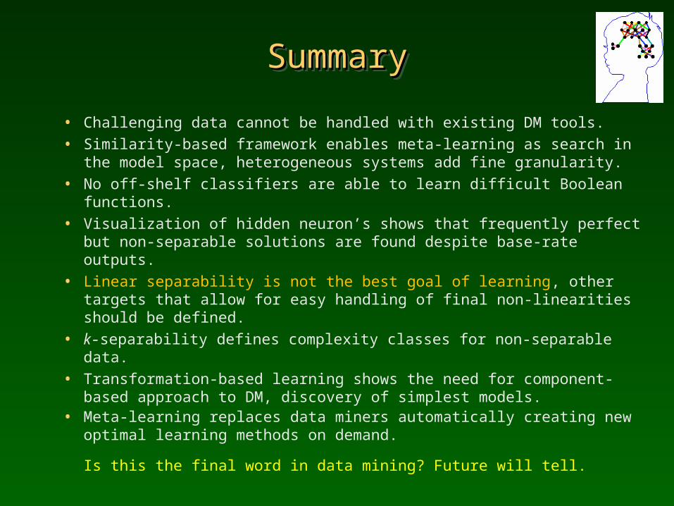
• Challenging data cannot be handled with existing DM tools. • Similarity-based framework enables meta-learning as search in the model

space, heterogeneous systems add fine granularity.• No off-shelf classifiers are able to learn difficult Boolean functions.• Visualization of hidden neuron’s shows that frequently perfect but non-

separable solutions are found despite base-rate outputs.• Linear separability is not the best goal of learning, other targets that allow

for easy handling of final non-linearities should be defined.• k-separability defines complexity classes for non-separable data. • Transformation-based learning shows the need for component-based

approach to DM, discovery of simplest models. • Meta-learning replaces data miners automatically creating new optimal

learning methods on demand.

Is this the final word in data mining? Future will tell.

Work like a horse Work like a horse butbut never loose your enthusiasm! never loose your enthusiasm!

Thank Thank youyoufor for

lending lending your your ears ears

......

Google: W. Duch => Papers & presentations; Norbert: http://www.is.umk.pl/~norbert/metalearning.html KIS: http://www.is.umk.pl => On-line publications.

Book: Meta-learning in Computational Intelligence (2010).