metabolic networks, reconstruction and analysis · metabolic networks, reconstruction and analysis...
TRANSCRIPT

Metabolic modellingMetabolic networks, reconstruction and analysis
Esa Pitkanen
Computational Methods for Systems Biology
1 December 2009
Department of Computer Science, University of Helsinki
Metabolic modelling – p. 1

Outline: Metabolism
Metabolism, metabolic networks
Metabolic reconstruction
Flux balance analysis
A part of the lecture material has been borrowed from JuhoRousu’s Metabolic modelling course!
Metabolic modelling – p. 2

What is metabolism?
Metabolism (from Greek "Metabolismos" for "change",or "overthrow") is the set of chemical reactions thathappen in living organisms to maintain life (Wikipedia)
Metabolic modelling – p. 3

What is metabolism?
Metabolism (from Greek "Metabolismos" for "change",or "overthrow") is the set of chemical reactions thathappen in living organisms to maintain life (Wikipedia)
Metabolism relates to various processes within the bodythat convert food and other substances into energy andother metabolic byproducts used by the body.
Cellular subsystem that processes small molecules ormetabolites to generate energy and building blocks forlarger molecules.
Metabolic modelling – p. 3
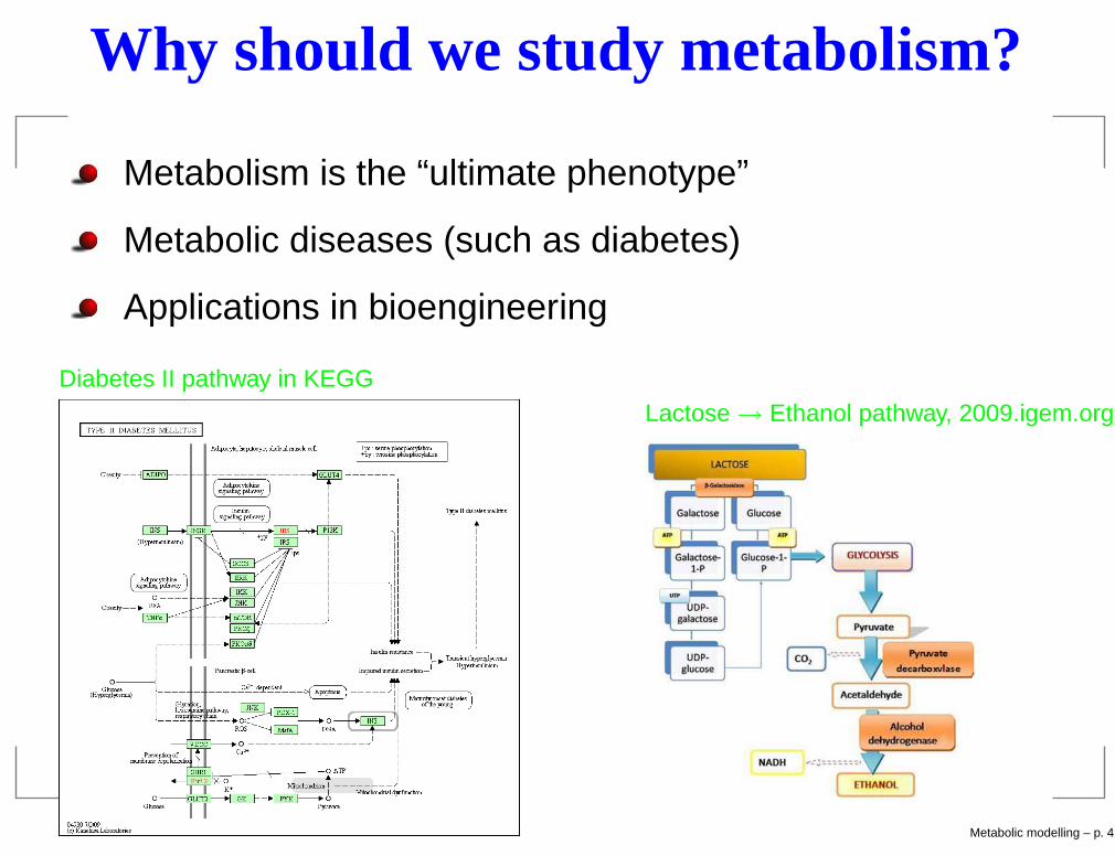
Why should we study metabolism?
Metabolism is the “ultimate phenotype”
Metabolic diseases (such as diabetes)
Applications in bioengineering
Diabetes II pathway in KEGGLactose→ Ethanol pathway, 2009.igem.org
Metabolic modelling – p. 4

Cellular space
Density of biomoleculesin the cell is high: plentyof interactions!
Figure: Escherichia colicross-section
Green: cell wallBlue, purple:cytoplasmic areaYellow: nucleoidregionWhite: mRNAm Image: David S. Goodsell
Metabolic modelling – p. 5
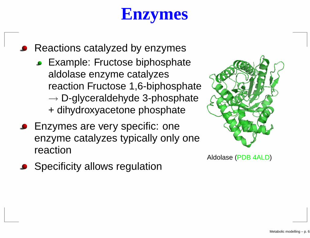
Enzymes
Reactions catalyzed by enzymesExample: Fructose biphosphatealdolase enzyme catalyzesreaction Fructose 1,6-biphosphate→ D-glyceraldehyde 3-phosphate+ dihydroxyacetone phosphate
Enzymes are very specific: oneenzyme catalyzes typically only onereaction
Specificity allows regulationAldolase (PDB 4ALD)
Metabolic modelling – p. 6

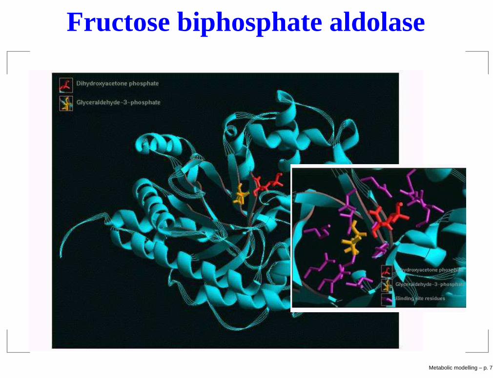
Fructose biphosphate aldolase
Metabolic modelling – p. 7
Fructose biphosphate aldolase
Metabolic modelling – p. 7

Metabolism: an overview
enzyme
metabolite
Metabolic modelling – p. 8

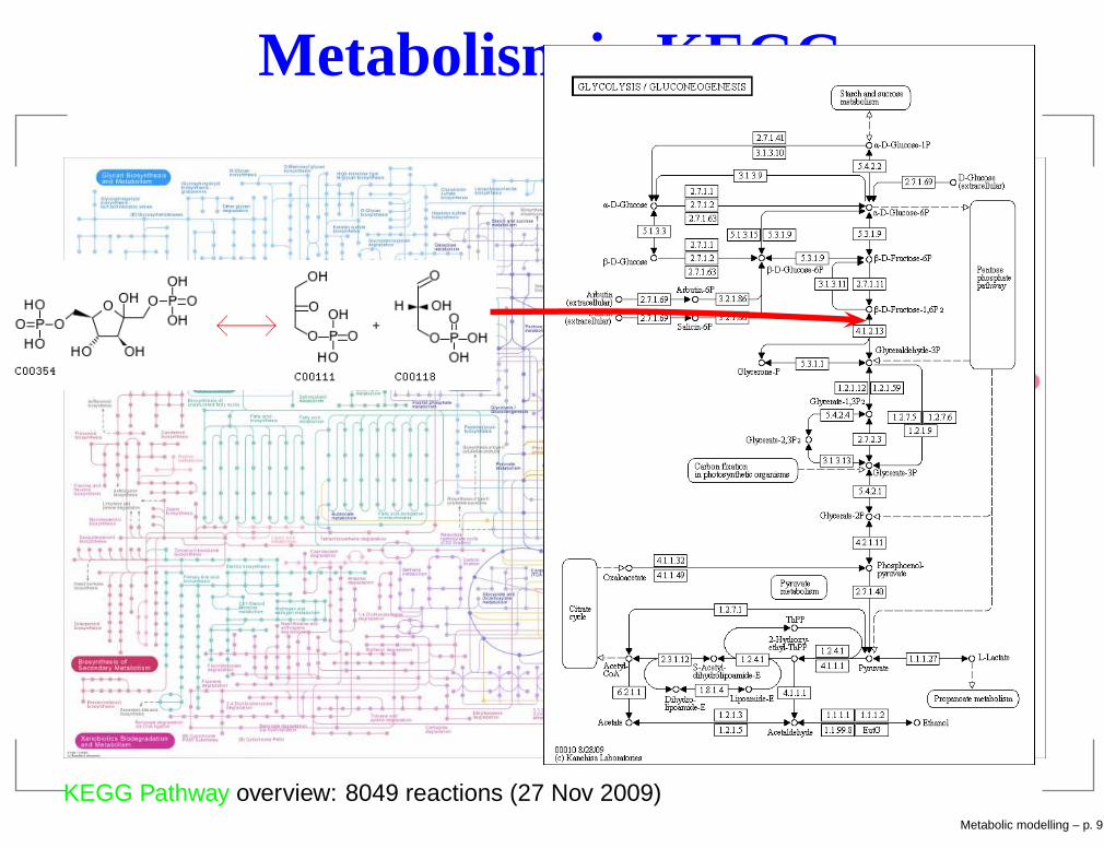
Metabolism in KEGG
KEGG Pathway overview: 8049 reactions (27 Nov 2009)Metabolic modelling – p. 9

Metabolism in KEGG
KEGG Pathway overview: 8049 reactions (27 Nov 2009)Metabolic modelling – p. 9
Metabolism in KEGG
KEGG Pathway overview: 8049 reactions (27 Nov 2009)Metabolic modelling – p. 9
Metabolic networks
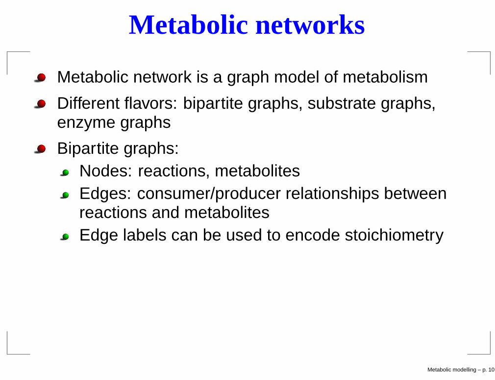
Metabolic network is a graph model of metabolism
Different flavors: bipartite graphs, substrate graphs,enzyme graphs
Bipartite graphs:Nodes: reactions, metabolitesEdges: consumer/producer relationships betweenreactions and metabolitesEdge labels can be used to encode stoichiometry
Metabolic modelling – p. 10

Metabolic networks
Metabolic network is a graph model of metabolism
Different flavors: bipartite graphs, substrate graphs,enzyme graphs
Bipartite graphs:Nodes: reactions, metabolitesEdges: consumer/producer relationships betweenreactions and metabolitesEdge labels can be used to encode stoichiometry
r1
6PGL
NADPH
r2
6PG
r3 R5P r4 X5P
r5 bG6P
r6 bF6P
r7r8 aG6P
r9r10 NADPP
H2O
Metabolic modelling – p. 10

Stoichiometric matrix
The stoichiometric coefficient sij of metabolite i inreaction j specifies the number of metabolites producedor consumed in a single reaction step
sij > 0: reaction produces metabolitesij < 0: reaction consumes metabolitesij = 0: metabolite does not participate in reaction
Example reaction: 2 m1 → m2 + m3
Coefficients: s1,1 = −2, s2,1 = s3,1 = 1
Coefficients comprise a stoichiometric matrix S = (sij).
Metabolic modelling – p. 11

Systems equations
Rate of concentration changes determined by the set ofsystems equations:
dxi
dt=
∑
j
sijvj ,
xi: concentration of metabolite i
sij: stoichiometric coefficientvj: rate of reaction j
Metabolic modelling – p. 12

Stoichiometric matrix: example
r1
6PGL
NADPH
r2
6PG
r3 R5P r4 X5P
r5 bG6P
r6 bF6P
r7r8 aG6P
r9r10 NADPP
H2O
r1 r2 r3 r4 r5 r6 r7 r8 r9 r10 r11 r12
βG6P -1 0 0 0 1 0 -1 0 0 0 0 0
αG6P 0 0 0 0 -1 -1 0 1 0 0 0 0
βF6P 0 0 0 0 0 1 1 0 0 0 0 0
6PGL 1 -1 0 0 0 0 0 0 0 0 0 0
6PG 0 1 -1 0 0 0 0 0 0 0 0 0
R5P 0 0 1 -1 0 0 0 0 0 0 0 0
X5P 0 0 0 1 0 0 0 0 -1 0 0 0
NADP+ -1 0 -1 0 0 0 0 0 0 1 0 0
NADPH 1 0 1 0 0 0 0 0 0 0 1 0
H2O 0 -1 0 0 0 0 0 0 0 0 0 1Metabolic modelling – p. 13

Modelling metabolism:kinetic models
Dynamic behaviour: how metabolite and enzymeconcentrations change over time → Kinetic models
Detailed models for individual enzymes
For simple enzymes, the Michaelis-Menten equationdescribes the reaction rate v adequately:
v =vmax[S]
KM + [S],
where vmax is the maximum reaction rate, [S] is thesubstrate concentration and KM is the Michaelisconstant.
Metabolic modelling – p. 14

Kinetic models
Require a lot of data to specify10-20 parameter models for more complex enzymes
Limited to small to medium-scale models
Metabolic modelling – p. 15
Spatial modelling
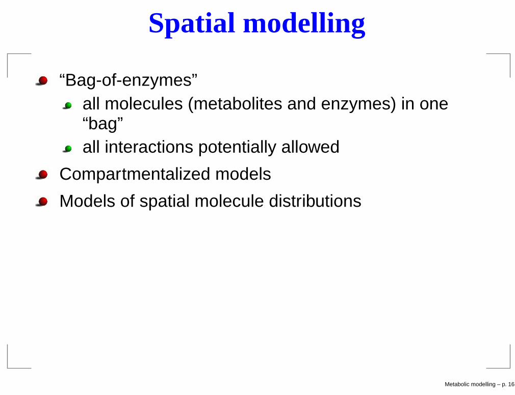
“Bag-of-enzymes”all molecules (metabolites and enzymes) in one“bag”all interactions potentially allowed
Compartmentalized models
Models of spatial molecule distributions
Metabolic modelling – p. 16

Spatial modelling
“Bag-of-enzymes”all molecules (metabolites and enzymes) in one“bag”all interactions potentially allowed
Compartmentalized models
Models of spatial molecule distributions
Incr
easi
ngde
tail
Metabolic modelling – p. 16

Compartments
Metabolic models of eukaryotic cells are divided intocompartments
CytosolMitochondriaNucleus...and others
Extracellular space can be thought as a “compartment”too
Metabolites carried across compartment borders bytransport reactions
Metabolic modelling – p. 17
Modelling metabolism: steady-state models
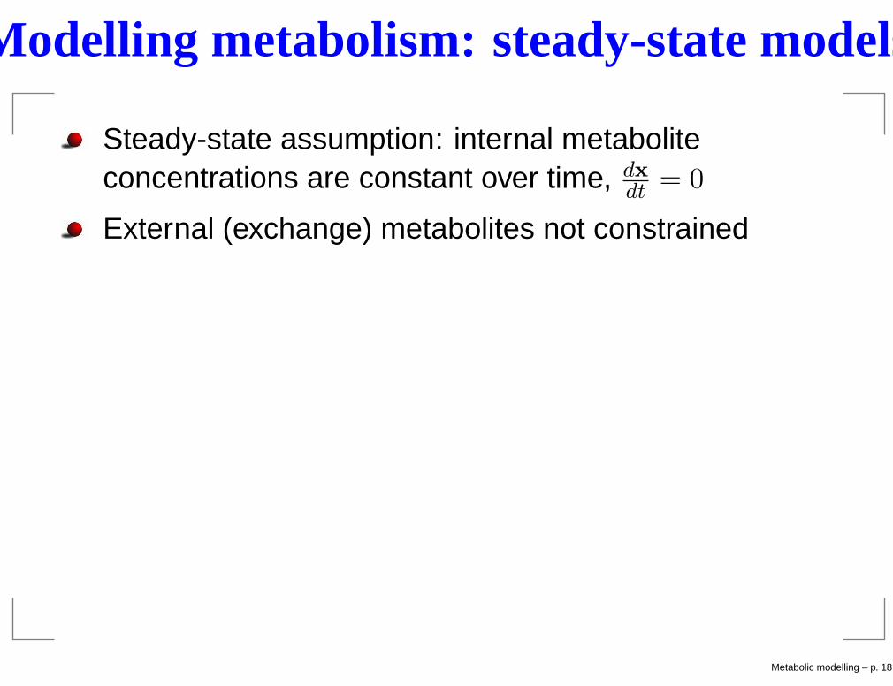
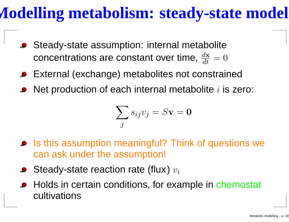
Steady-state assumption: internal metaboliteconcentrations are constant over time, dx
dt= 0
External (exchange) metabolites not constrained
Metabolic modelling – p. 18

Modelling metabolism: steady-state models
Steady-state assumption: internal metaboliteconcentrations are constant over time, dx
dt= 0
External (exchange) metabolites not constrained
Net production of each internal metabolite i is zero:∑
j
sijvj = Sv = 0
Is this assumption meaningful? Think of questions wecan ask under the assumption!
Metabolic modelling – p. 18
Modelling metabolism: steady-state models
Steady-state assumption: internal metaboliteconcentrations are constant over time, dx
dt= 0
External (exchange) metabolites not constrained
Net production of each internal metabolite i is zero:∑
j
sijvj = Sv = 0
Is this assumption meaningful? Think of questions wecan ask under the assumption!
Steady-state reaction rate (flux) vi
Holds in certain conditions, for example in chemostatcultivations
Metabolic modelling – p. 18
Outline: Metabolic reconstruction
Metabolism, metabolic networks
Metabolic reconstruction
Flux balance analysis
Metabolic modelling – p. 19

Metabolic reconstruction
Reconstruction problem: infer the metabolic networkfrom sequenced genome
Determine genes coding for enzymes and assemblemetabolic network?
Subproblem of genome annotation?
Metabolic modelling – p. 20

Metabolic reconstruction
Metabolic modelling – p. 21

Reconstruction process
Metabolic modelling – p. 22

Data sources for reconstruction
BiochemistryEnzyme assays: measure enzymatic activity
GenomicsAnnotation of open reading frames
PhysiologyMeasure cellular inputs (growth media) and outputsBiomass composition
Metabolic modelling – p. 23
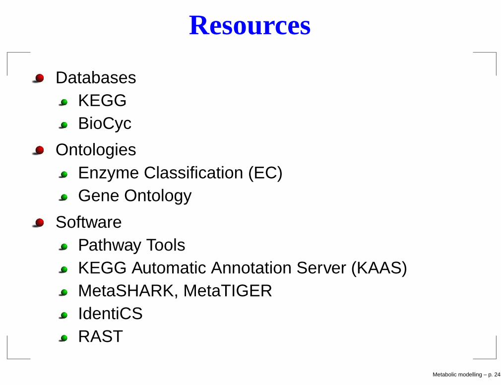
Resources
DatabasesKEGGBioCyc
OntologiesEnzyme Classification (EC)Gene Ontology
SoftwarePathway ToolsKEGG Automatic Annotation Server (KAAS)MetaSHARK, MetaTIGERIdentiCSRAST
Metabolic modelling – p. 24

Annotating sequences
1. Find genes in sequenced genome (available software)GLIMMER (microbes)GlimmerM (eukaryotes, considers intron/exonstructure)GENSCAN (human)
2. Assign a function to each geneBLAST, FASTA against a database of annotatedsequences (e.g., UniProt)Profile-based methods (HMMs, see InterProScan fora unified interface for different methods)Protein complexes, isozymes
Metabolic modelling – p. 25

Assembling the metabolic network
In principle: for each gene withannotated enzymatic function(s),add reaction(s) to network(gene-protein-reaction associations)
Metabolic modelling – p. 26

Assembling the metabolic network
In principle: for each gene withannotated enzymatic function(s),add reaction(s) to network(gene-protein-reaction associations)
Multiple peptides may form a singleprotein (top)
Proteins may form complexes(middle)
Different genes may encodeisozymes (bottom)
Reed et al., GenomeMetabolic modelling – p. 26

Gaps in metabolic networks
Assembled network often contains so-called gaps
Informally: gap is a reaction“missing” from the network......required to perform some function.
A large amount of manual work is required to fixnetworks
Recently, computational methods have been developedto fix network consistency problems
Metabolic modelling – p. 27

Gaps in metabolic networks
May carry steady-state flux – Blocked – Gap
r1
6PGL
NADPH
r2
6PG
r3 R5P r4 X5P
r5 bG6P
r6 bF6P
r7r8 aG6P
r9r10 NADPP
H2O
Metabolic modelling – p. 28

Gaps in metabolic networks
May carry steady-state flux – Blocked – Gap
r1
6PGL
NADPH
r2
6PG
r3 R5P r4 X5P
r5 bG6P
r6 bF6P
r7r8 aG6P
r9r10 NADPP
H2O
r1
6PGL
NADPH
r2
6PG
r3 R5P r4 X5P
r5 bG6P
r6 bF6P
r7r8 aG6P
r9r10 NADPP
H2O
Metabolic modelling – p. 28

Gaps in metabolic networks
May carry steady-state flux – Blocked – Gap
r1
6PGL
NADPH
r2
6PG
r3 R5P r4 X5P
r5 bG6P
r6 bF6P
r7r8 aG6P
r9r10 NADPP
H2O
r1
6PGL
NADPH
r2
6PG
r3 R5P r4 X5P
r5 bG6P
r6 bF6P
r7r8 aG6P
r9r10 NADPP
H2O
r1
6PGL
NADPH
r2
6PG
r3 R5P r4 X5P
r5 bG6P
r6 bF6P
r7r8 aG6P
r9r10 NADPP
H2O
Metabolic modelling – p. 28

In silico validation of metabolic models
Reconstructed genome-scale metabolic networks arevery large: hundreds or thousands of reactions andmetabolites
Manual curation is often necessary
Amount of manual work needed can be reduced withcomputational methods
Aims to provide a good basis for further analysis andexperiments
Does not remove the need for experimental verification
Metabolic modelling – p. 29

Outline: Flux balance analysis
Metabolism, metabolic networks
Metabolic reconstruction
Flux balance analysis
Metabolic modelling – p. 30

Flux Balance Analysis: preliminaries
Recall that in a steady state, metabolite concentrationsare constant over time,
dxi
dt=
r∑
j=1
sijvj = 0, for i = 1, . . . , n.
Stoichiometric model can be given as
S = [SII SIE ]
where SII describes internal metabolites - internalreactions, and SIE internal metabolites - exchangereactions.
Metabolic modelling – p. 31

Flux Balance Analysis (FBA)
FBA is a framework for investigating the theoreticalcapabilities of a stoichiometric metabolic model S
Analysis is constrained by1. Steady state assumption Sv = 0
2. Thermodynamic constraints: (ir)reversibility ofreactions
3. Limited reaction rates of enzymes: Vmin ≤ v ≤ Vmax
Note that constraints (2) can be included in Vmin andVmax.
Metabolic modelling – p. 32
Flux Balance Analysis (FBA)
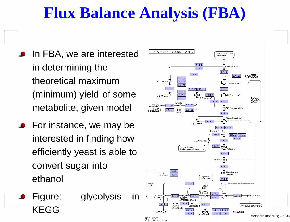
In FBA, we are interestedin determining thetheoretical maximum(minimum) yield of somemetabolite, given model
For instance, we may beinterested in finding howefficiently yeast is able toconvert sugar intoethanol
Figure: glycolysis inKEGG
Metabolic modelling – p. 33

Flux Balance Analysis (FBA)
FBA has applications both in metabolic engineering andmetabolic reconstruction
Metabolic engineering: find out possible reactions(pathways) to insert or delete
Metabolic reconstruction: validate the reconstructiongiven observed metabolic phenotype
Metabolic modelling – p. 34

Formulating an FBA problem
We formulate an FBA problem by specifying parametersc in the optimization function Z,
Z =r∑
i=1
civi.
Examples:Set ci = 1 if reaction i produces “target” metabolite,and ci = 0 otherwiseGrowth function: maximize production of biomassconstituentsEnergy: maximize ATP (net) production
Metabolic modelling – p. 35

Solving an FBA problem
Given a model S, we then seek to find the maximum ofZ while respecting the FBA constraints,
maxv
Z = maxv
r∑
i=1
civi such that(1)
Sv = 0(2)
Vmin ≤ v ≤ Vmax(3)
(We could also replace max with min.)
This is a linear program, having a linear objectivefunction and linear constraints
Metabolic modelling – p. 36

Solving a linear program
General linear program formulation:
maxxi
∑
i
cixi such that
Ax ≤ b
Algorithms: simplex (worst-case exponential time),interior point methods (polynomial)
Matlab solver: linprog (Statistical Toolbox)
Many solvers around, efficiency with (very) largemodels varies
Metabolic modelling – p. 37

Linear programs
Linear constraints define aconvex polyhedron (feasibleregion)
If the feasible region isempty, the problem isinfeasible.
Unbounded feasible region(in direction of objectivefunction): no optimal solution
Given a linear objective func-tion, where can you find themaximum value?
Metabolic modelling – p. 38
Flux Balance Analysis: example
r1
6PGL
NADPH
r2
6PG
r3 R5P r4 X5P
r5 bG6P
r6 bF6P
r7r8 aG6P
r9r10 NADPP
H2O
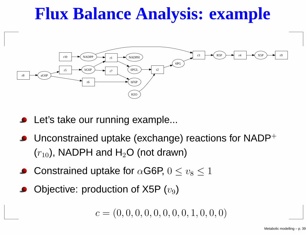
Let’s take our running example...
Unconstrained uptake (exchange) reactions for NADP+
(r10), NADPH and H2O (not drawn)
Constrained uptake for αG6P, 0 ≤ v8 ≤ 1
Objective: production of X5P (v9)
c = (0, 0, 0, 0, 0, 0, 0, 0, 1, 0, 0, 0)
Metabolic modelling – p. 39

Flux Balance Analysis: example
r1
6PGL
NADPH
r2
6PG
r3 R5P r4 X5P
r5 bG6P
r6 bF6P
r7r8 aG6P
r9r10 NADPP
H2O
r1 r2 r3 r4 r5 r6 r7 r8 r9 r10 r11 r12
βG6P -1 0 0 0 1 0 -1 0 0 0 0 0
αG6P 0 0 0 0 -1 -1 0 1 0 0 0 0
βF6P 0 0 0 0 0 1 1 0 0 0 0 0
6PGL 1 -1 0 0 0 0 0 0 0 0 0 0
6PG 0 1 -1 0 0 0 0 0 0 0 0 0
R5P 0 0 1 -1 0 0 0 0 0 0 0 0
X5P 0 0 0 1 0 0 0 0 -1 0 0 0
NADP+ -1 0 -1 0 0 0 0 0 0 1 0 0
NADPH 1 0 1 0 0 0 0 0 0 0 1 0
H2O 0 -1 0 0 0 0 0 0 0 0 0 1Metabolic modelling – p. 40
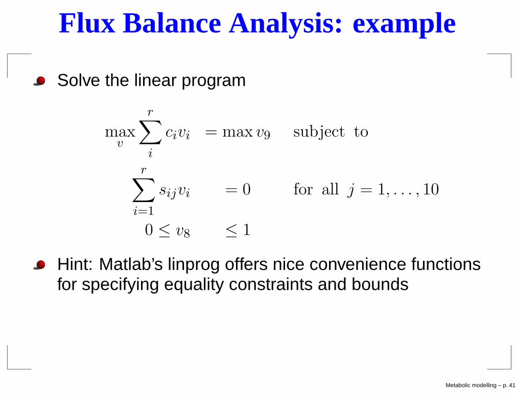
Flux Balance Analysis: example
Solve the linear program
maxv
r∑
i
civi = max v9 subject to
r∑
i=1
sijvi = 0 for all j = 1, . . . , 10
0 ≤ v8 ≤ 1
Hint: Matlab’s linprog offers nice convenience functionsfor specifying equality constraints and bounds
Metabolic modelling – p. 41

Flux Balance Analysis: example
r1 1.00
6PGL
NADPH
r2 1.00
6PG
r3 1.00 R5P r4 1.00 X5P
r5 0.57 bG6P
r6 0.43 bF6P
r7 -0.43r8 1.00 aG6P
r9 1.00r10 2.00 NADPP
H2O
Figure gives one possible solution (flux assignment v)
Reaction r7 (red) operates in backward direction
Uptake of NADP+ v10 = 2v8 = 2
How many solutions (different flux assignments) arethere for this problem?
Metabolic modelling – p. 42
FBA validation of a reconstruction
Check if it is possible to produce metabolites that theorganism is known to produce
Maximize production of each such metabolite at timeMake sure max. production is above zero
To check biomass production (growth), add a reactionto the model with stoichiometry corresponding tobiomass composition
Metabolic modelling – p. 43

FBA validation of a reconstruction
If a maximum yield of some metabolite is lower thanmeasured → missing pathway
Iterative process: find metabolite that cannot beproduced, fix the problem by changing the model, tryagain
r1 0.00
6PGL
NADPH
r2 0.00 6PG
r3 0.00 R5P r4 0.00 X5P
r5 0.00 bG6P
r6 0.00 bF6P
r7 0.00
r8 0.00 aG6P
r9 0.00
NADPP
H2O
r1 1.00
6PGL
NADPH
r2 1.00
6PG
r3 1.00 R5P r4 1.00 X5P
r5 0.57 bG6P
r6 0.43 bF6P
r7 -0.43r8 1.00 aG6P
r9 1.00r10 2.00 NADPP
H2OMetabolic modelling – p. 44

FBA validation of a reconstruction
FBA gives the maximum flux given stoichiometry only,i.e., not constrained by regulation or kinetics
In particular, assignment of internal fluxes on alternativepathways can be arbitrary (of course subject to problemconstraints)
r1 1.00
6PGL
NADPH
r2 1.00
6PG
r3 1.00 R5P r4 1.00 X5P
r5 0.57 bG6P
r6 0.43 bF6P
r7 -0.43r8 1.00 aG6P
r9 1.00r10 2.00 NADPP
H2O
r1 1.00
6PGL
NADPH
r2 1.00
6PG
r3 1.00 R5P r4 1.00 X5P
r5 0.00 bG6P
r6 1.00 bF6P
r7 -1.00r8 1.00 aG6P
r9 1.00r10 2.00 NADPP
H2OMetabolic modelling – p. 45

Further reading
Metabolic modelling: course material
M. Durot, P.-Y. Bourguignon, and V. Schachter:
Genome-scale models of bacterial metabolism: ... FEMS
Microbiol Rev. 33:164-190, 2009.
N. C. Duarte et. al : Global reconstruction of the human
metabolic network based on genomic and bibliomic data.
PNAS 104(6), 2007.
V. Lacroix, L. Cottret, P. Thebault and M.-F. Sagot: An
introduction to metabolic networks and their structural analysis.
IEEE Transactions on Computational Biology and
Bioinformatics 5(4), 2008.
E. Pitkänen, A. Rantanen, J. Rousu and E. Ukkonen:
A computational method for reconstructing gapless metabolic networks.
Proceedings of the BIRD’08, 2008.Metabolic modelling – p. 46