Metaheuristic Techniques

Sunith Bandarua, Kalyanmoy Debb

aSchool of Engineering Science, University of Skovde, Skovde 541 28, SwedenbDepartment of Electrical and Computer Engineering, Michigan State University,

East Lansing, 428 S. Shaw Lane, 2120 EB, MI 48824, USA

COIN Report Number 2016029*

Abstract

Most real-world search and optimization problems involve complexities such as non-convexity, non-linearities, discontinuities, mixed nature of variables, multiple disciplines and large dimensionality, acombination of which renders classical provable algorithms to be either ineffective, impractical or inap-plicable. There do not exist any known mathematically motivated algorithms for finding the optimalsolution for all such problems in a limited computational time. Thus, in order to solve such problemsto practicality, search and optimization algorithms are usually developed using certain heuristics thatthough lacking in strong mathematical foundations, are nevertheless good at reaching an approximatesolution in a reasonable amount of time. These so-called metaheuristic methods do not guarantee findingthe exact optimal solution, but can lead to a near-optimal solution in a computationally efficient manner.Due to this practical appeal combined with their ease of implementation, metaheuristic methodologies aregaining popularity in several application domains. Most metaheuristic methods are stochastic in natureand mimic a natural, physical or biological principle resembling a search or an optimization process. Inthis paper, we discuss a number of such methodologies, specifically evolutionary algorithms, such as ge-netic algorithms and evolution strategy, particle swarm optimization, ant colony optimization, bee colonyoptimization, simulated annealing and a host of other methods. Many metaheuristic methodologies arebeing proposed by researchers all over the world on a regular basis. It therefore becomes important tounify them to understand common features of different metaheuristic methods and simultaneously tostudy fundamental differences between them. Hopefully, such endeavors will eventually allow a user tochoose the most appropriate metaheuristic method for the problem at hand.

1. Introduction

The present paper does not claim to be a thorough survey of all existing metaheuristic methods andtheir related aspects. Instead, the purpose is to describe some of the most popular methods and providepseudocodes to enable beginners to easily implement them. Therefore, this paper should be seen moreas a quick-start guide to popular metaheuristics than as a survey of methods and applications. Readersinterested in the history, variants, empirical analysis, specific applications, tuning and parallelization ofmetaheuristic methods should refer to the following texts:

1. Books: [1, 2, 3, 4, 5, 6, 7, 8, 9, 10, 11, 12, 13]2. Surveys: [14, 15, 16, 17, 18, 19, 20, 21, 22, 23, 24]3. Combinatorial Problems: [25, 26, 27, 28, 29, 30, 31, 32, 33, 34]4. Analysis: [35, 36, 37, 38, 39, 40, 41, 42, 43]

∗Published in Decision Sciences: Theory and Practice, Edited by Raghu Nandan Sengupta, Aparna Gupta and JoydeepDutta, 693–750, CRC Press, Taylor & Francis Group.

Email addresses: sunith.bandaru@his.se (Sunith Bandaru), kdeb@egr.msu.edu (Kalyanmoy Deb)

1

5. Parallelization: [44, 45, 46, 47, 48, 49, 50, 51, 52].

The development of new metaheuristic methods has picked up pace over the last 20 years. Nowadays,many conferences, workshops, symposiums and journals accept submissions related to this topic. Someof them (in no particular order) are:

Conferences/Symposiums:1. Genetic and Evolutionary Computation Conference (GECCO)2. IEEE Congress on Evolutionary Computation (CEC)3. Evolutionary Multi-criterion Optimization (EMO)4. Parallel Problem Solving from Nature (PPSN)5. Foundations of Genetic Algorithms (FOGA)6. Simulated Evolution And Learning (SEAL)7. Learning and Intelligent OptimizatioN (LION)8. International Joint Conference on Computational Intelligence (IJCCI)9. International Conference on Artificial Intelligence and Soft Computing (ICAISC)

10. IEEE Symposium Series on Computational Intelligence (SSCI)11. IEEE Swarm Intelligence Symposium (SIS)

Journals:1. IEEE Transactions on Evolutionary Computation (IEEE Press)2. Applied Soft Computing (Elsevier)3. Computers & Operations Research (Elsevier)4. European Journal of Operational Research (Elsevier)5. Information Sciences (Elsevier)6. Evolutionary Computation (MIT Press)7. Computational Optimization and Applications (Springer)8. Soft Computing (Springer)9. Engineering Optimization (Taylor & Francis)

10. IEEE Transactions on Systems, Mans and Cybernetics (IEEE Press)11. Engineering Applications of Artificial Intelligence (Elsevier)12. International Transactions in Operational Research (Wiley)13. Intelligent Automation & Soft Computing (Taylor & Francis)14. Applied Computational Intelligence and Soft Computing (Hindawi)15. Journal of Multi-Criteria Decision Analysis (Wiley)16. Artificial Life (MIT Press)17. Journal of Mathematical Modelling and Algorithms in Operations Research (Springer, Discontin-

ued)18. International journal of Artificial Intelligence & Applications (AIRCC)

Some publications that are entirely dedicated to metaheuristics also exist, namely,

1. Journal of Heuristics (Springer)2. Swarm and Evolutionary Computation (Elsevier)3. Swarm Intelligence (Springer)4. Natural Computing (Springer)5. Genetic Programming and Evolvable Machines (Springer)6. International Journal of Metaheuristics (Inderscience)7. International Journal of Bio-Inspired Computation (Inderscience)8. Memetic Computing (Springer)9. International Journal of Applied Metaheuristic Computing (IGI Global)

10. Computational Intelligence and Metaheuristic Algorithms with Applications (Hindawi)11. European Event on Bio-Inspired Computation (EvoStar Conference)

2

12. International Conference on Adaptive & Natural Computing Algorithms (ICANNGA)13. Ant Colony Optimization and Swarm Intelligence (ANTS Conference)14. Swarm, Evolutionary and Memetic Computing Conference (SEMCCO)15. Bio-Inspired Computing: Theories and Applications (BICTA)16. Nature and Biologically Inspired Computing (NaBIC)17. International Conference on Soft Computing for Problem Solving (SocProS)18. Metaheuristics International Conference (MIC)19. International Conference on Metaheuristics and Nature Inspired Computing (META Conference)

Implementation of metaheuristic methods, though mostly straightforward, can be a tedious task.Luckily, several software frameworks are freely available on the internet which can be used by beginnersto get started with solving their optimization problems. Notable examples are:

1. PISA: A platform and programming language independent interface for search algorithms(http://www.tik.ee.ethz.ch/pisa/)

2. ParadisEO: A C++ software framework for metaheuristics(http://paradiseo.gforge.inria.fr/)

3. Open BEAGLE: A C++ evolutionary computation framework(https://code.google.com/p/beagle/)

4. Evolving Objects: An evolutionary computation framework(http://eodev.sourceforge.net/)

5. GAlib: A C++ library of genetic algorithm components(http://lancet.mit.edu/ga/)

6. METSlib: A metaheuristic modeling framework and optimization toolkit in C++(https://projects.coin-or.org/metslib)

7. ECF: A C++ evolutionary computation framework(http://gp.zemris.fer.hr/ecf/)

8. HeuristicLab: A framework for heuristic and evolutionary algorithms(http://dev.heuristiclab.com/)

9. ECJ: A Java-based evolutionary computation research system(https://cs.gmu.edu/~eclab/projects/ecj/)

10. jMetal: Metaheuristic algorithms in Java(http://jmetal.sourceforge.net/)

11. MOEA Framework: A free and open source Java framework for multiobjective optimization(http://www.moeaframework.org/)

12. JAMES: A Java metaheuristics search framework(http://www.jamesframework.org/)

13. Watchmaker Framework: An object-oriented framework for evolutionary/genetic algorithms in Java(http://watchmaker.uncommons.org/)

14. Jenetics: An evolutionary algorithm library written in Java(http://jenetics.io/)

15. Pyevolve: A complete genetic algorithm framework in Python(http://pyevolve.sourceforge.net/)

16. DEAP: Distributed evolutionary algorithms in Python(https://github.com/DEAP/deap)

These implementations provide the basic framework required to run any of the several available meta-heuristics. Software implementations specific to individual methods are also available in plenty. Forexample, genetic programming (discussed later in Section 10) which requires special solution representa-tion schemes, has several variants in different programming languages, each handling the representationin a unique way.

This paper is arranged as follows. In the next section, we discuss basic concepts and classification ofmetaheuristics. We also lay down a generic metaheuristic framework which covers most of the available

3

methods. From Section 3 to Section 14 we cover several popular metaheuristic techniques with completepseudocodes. We discuss the methods in alphabetical order in order to avoid preconceptions aboutperformance, generality and applicability, thus respecting the No Free Lunch theorem [53] of optimization.In Section 15, we enumerate several less popular methods with a brief description of their origins. Thesemethodologies are ordered by their number of Google Scholar citations. We conclude this paper inSection 16 with a few pointers to future research directions.

2. Concepts of Metaheuristic Techniques

The word ‘heuristic’ is defined in the context of computing as a method of denoting a rule-of-thumbfor solving a problem without the exhaustive application of a procedure. In other words, a heuristicmethod is one that (i) looks for an approximate solution, (ii) need not particularly have a mathematicalconvergence proof, and (iii) does not explore each and every possible solution in the search space beforearriving at the final solution, hence is computationally efficient.

A metaheuristic method is particularly relevant in the context of solving search and optimizationproblems. It describes a method that uses one or more heuristics and therefore inherits all the threeproperties mentioned above. Thus, a metaheuristic method (i) seeks to find a near-optimal solution,instead of specifically trying to find the exact optimal solution, (ii) usually has no rigorous proof ofconvergence to the optimal solution, and (iii) is usually computationally faster than exhaustive search.These methods are iterative in nature and often use stochastic operations in their search process tomodify one or more initial candidate solutions (usually generated by random sampling of the searchspace). Since many real-world optimization problems are complex due to their inherent practicalities,classical optimization algorithms may not always be applicable and may not fair well in solving suchproblems in a pragmatic manner. Realizing this fact and without disregarding the importance of classicalalgorithms in the development of the field of search and optimization, researchers and practitioners soughtfor metaheuristic methods so that a near-optimal solution can be obtained in a computationally tractablemanner, instead of waiting for a provable optimization algorithm to be developed before attempting tosolve such problems. The ability of the metaheuristic methods to handle different complexities associatedwith practical problems and arrive at a reasonably acceptable solution is the main reason for the popularityof metaheuristic methods in the recent past.

Most metaheuristic methods are motivated by natural, physical or biological principles and try tomimic them at a fundamental level through various operators. A common theme seen across all meta-heuristics is the balance between exploration and exploitation. Exploration refers to how well the operatorsdiversify solutions in the search space. This aspect gives the metaheuristic a global search behavior. Ex-ploitation refers to how well the operators are able to utilize the information available from solutionsfrom previous iterations to intensify search. Such intensification gives the metaheuristic a local searchcharacteristic. Some metaheuristics tend to be more explorative than exploitative, while some others dothe opposite. For example, the primitive method of randomly picking solutions for a certain number ofiterations, represents a completely explorative search. On the other hand, hill climbing where the currentsolution is incrementally modified until it improves, is an example of completely exploitative search. Morecommonly, metaheuristics allow this balance between diversification and intensification to be adjusted bythe user through operator parameters.

The characteristics described above give metaheuristics certain advantages over the classical optimiza-tion methods, namely,

1. Metaheuristics can lead to good enough solutions for computationally easy (technically, P class)problems with large input complexity, which can be a hurdle for classical methods.

2. Metaheuristics can lead to good enough solutions for the NP-hard problems, i.e. problems for whichno known exact algorithm exists that can solve them in a reasonable amount of time.

3. Unlike most classical methods, metaheuristics require no gradient information and therefore can beused with non-analytic, black-box or simulation-based objective functions.

4

4. Most metaheuristics have the ability to recover from local optima due to inherent stochasticity ordeterministic heuristics specifically meant for this purpose.

5. Because of the ability to recover from local optima, metaheuristics can better handle uncertaintiesin objectives.

6. Most metaheuristics can handle multiple objectives with only a few algorithmic changes.

2.1. Optimization Problems

A non-linear programming (NLP) problem involving n real or discrete (integer, boolean or otherwise)variables or a combination thereof is stated as follows:

Minimize f(x),subject to gj(x) ≥ 0, j = 1, 2, . . . , J,

hk(x) = 0, k = 1, 2, . . . ,K,

x(L)i ≤ xi ≤ x(U)

i , i = 1, 2, . . . , n,

(1)

where f(x) is the objective function to be optimized, gj(x) represent J inequality constraints and hk(x)represent K equality constraints. Typically, equality constraints are handled by converting them intosoft inequality constraints. A survey of constraint handling methods can be found in [54, 55]. A solution

x is feasible if all J +K constraints and variable bounds [x(L)i , x

(U)i ] are satisfied.

The nature of the optimization problem plays an important role in determining the optimizationmethodology to be used. Classical optimization methods should always be the first choice for solvingconvex problems. An NLP problem is said to be convex if and only if, (i) f is convex, (ii) all gj(x)are concave, and (iii) all hk(x) are linear. Unfortunately, most real-world problems are non-convex andNP-hard, which makes metaheuristic techniques a popular choice.

Metaheuristics are especially popular for solving combinatorial optimization problems because notmany classical methods can handle the kind of variables that they involve. A typical combinatorialoptimization problem involves an n-dimensional permutation p in which every entity appears only once:

Minimize f(p),subject to gj(p) ≥ 0, j = 1, 2, . . . , J

hk(p) ≥ 0, k = 1, 2, . . . ,K.(2)

Again, a candidate permutation p is feasible only when all J constraints are satisfied. Many practicalproblems involve combinatorial optimization. Examples include knapsack problems, bin-packing, networkdesign, traveling salesman, vehicle routing, facility location and scheduling.

When multiple objectives are involved that conflict with each other, no single solution exists that cansimultaneously optimize all the objectives. Rather, a multitude of optimal solutions are possible whichprovide a trade-off between the objectives. These solutions are known as the Pareto-optimal solutionsand they lie on what is known as the Pareto-optimal front. A candidate solution x1 is said to dominatex2 and denoted as x1 ≺ x2 if and only if the following conditions are satisfied:

1. fi(x1) ≤ fi(x2) ∀i ∈ {1, 2, . . . ,m},2. and ∃j ∈ {1, 2, . . . ,m} such that fj(x1) < fj(x2).

If only the first of these conditions is satisfied then x1 is said to weakly dominate x2 and is denoted asx1 � x2. If neither x1 � x2 nor x2 � x1, then x1 and x2 are said to be non-dominated with respect toeach other and denoted as x1||x2. A feasible solution x∗ is said to be Pareto-optimal if there does notexist any other feasible x such that x ≺ x∗. The set of all such x∗ (which are non-dominated with respectto each other) is referred to as the Pareto-optimal set. Multi-objective optimization poses additionalchallenges to metaheuristics due to this concept of non-dominance.

In this paper, we will restrict ourselves to describing metaheuristics in the context of single-objectiveoptimization. Most metaheuristics can be readily used for multi-objective optimization by simply con-sidering Pareto-dominance or other suitable selection mechanisms when comparing different solutions

5

and by taking extra measures for preserving solution diversity. However, it is important to note thatsince multi-objective optimization problems with conflicting objectives have multiple optimal solutions,metaheuristics that use a ‘population’ of solutions are preferred so that the entire Pareto-optimal frontcan be represented simultaneously.

2.2. Classification of Metaheuristic Techniques

The most common way of classifying metaheuristic techniques is based on the number of initialsolutions that are modified in subsequent iterations. Single-solution metaheuristics start with one initialsolution which gets modified iteratively. Note that the modification process itself may involve more thanone solution, but only a single solution is used in each following iteration. Population-based metaheuristicsuse more than one initial solution to start optimization. In each iteration, multiple solutions get modified,and some of them make it to the next iteration. Modification of solutions is done through operatorsthat often use special statistical properties of the population. The additional parameter for size of thepopulation is set by the user and usually remains constant across iterations.

Another way of classifying metaheuristics is through the domain that they mimic. Umbrella terms suchas bio-inspired and nature-inspired are often used for metaheuristics. However, they can be further sub-categorized as evolutionary algorithms, swarm-intelligence based algorithms and physical phenomenonbased algorithms. Evolutionary algorithms (like genetic algorithms, evolution strategies, differential evo-lution, genetic programming, evolutionary programming, etc.) mimic various aspects of evolution innature such as survival of the fittest, reproduction and genetic mutation. Swarm-intelligence algorithmsmimic the group behavior and/or interactions of living organisms (like ants, bees, birds, fireflies, glow-worms, fishes, white-blood cells, bacteria, etc.) and non-living things (like water drops, river systems,masses under gravity, etc.). The rest of the metaheuristics mimic various physical phenomena like an-nealing of metals, musical aesthetics (harmony), etc. A fourth sub-category may be used to classifymetaheuristics whose source of inspiration is unclear (like tabu search and scatter search) or those thatare too few in number to have a category for themselves.

Other popular ways of classifying metaheuristics are [1, 35]:

1. Deterministic versus stochastic methods: Deterministic methods follow a definite trajectory fromthe random initial solution(s). Therefore, they are sometimes referred to as trajectory methods.Stochastic methods (also discontinuous methods) allow probabilistic jumps from the current solu-tion(s) to the next.

2. Greedy versus non-greedy methods: Greedy algorithms usually search in the neighborhood of thecurrent solution and immediately move to a better solution when its found. This behavior oftenleads to a local optimum. Non-greedy methods either hold out for some iterations before updatingthe solution(s) or have a mechanism to back track from a local optimum. However, for convexproblems, a greedy behavior is the optimum strategy.

3. Memory usage versus memoryless methods: Memory-based methods maintain a record of pastsolutions and their trajectories and use them to direct search. A popular memory method calledtabu search will be discussed in Section 14.

4. One versus various neighborhood methods: Some metaheuristics like simulated annealing and tabusearch only allow a limited set of moves from the current solution. But many metaheuristicsemploy operators and parameters to allow multiple neighborhoods. For example, particle swarmoptimization achieves this through various swarm topologies.

5. Dynamic versus static objective function: Metaheuristics that update the objective function de-pending on the current requirements of search are classified as dynamic. Other metaheuristicssimply use their operators to control search.

Most metaheuristics are population-based, stochastic, non-greedy and use a static objective function.In this paper we avoid making any attempt at classifying individual metaheuristic techniques because

of two reasons:

6

1. Single-solution metaheuristics can often be transformed into population-based ones (and vice versa)either by hybridization with other methods or, sometimes, simply by consideration of multiple initialsolutions.

2. The large number of metaheuristics that have been derived off late from existing techniques usevarious modifications in their operators. Sometimes these variants blur the extent of mimicry somuch that referring to them by their domain of inspiration becomes unreasonable.

Therefore, for each metaheuristic, we discuss the most popular and generic variant.

2.3. A Generic Metaheuristic Framework

Most metaheuristics follow a similar sequence of operations and therefore can be defined within acommon generic framework as shown in Algorithm 1.

Algorithm 1 A Generic Metaheuristic Framework

Require: SP, GP, RP, UP, TP, N (≥ 1), µ (≤ N), λ, ρ (≤ N)1: Set iteration counter t = 02: Initialize N solutions St randomly3: Evaluate each member of St4: Mark the best solution of St as x∗t5: repeat6: Choose µ solutions (set Pt) from St using a selection plan (SP)7: Generate λ new solutions (set Ct) from Pt using a generation plan (GP)8: Choose ρ solutions (set Rt) from St using a replacement plan (RP)9: Update St by replacing Rt using ρ solutions from a pool of any combination of at most three sets

Pt, Ct, and Rt using an update plan (UP)10: Evaluate each member of St11: Identify the best solution of St and update x∗t12: t← t+ 113: until (a termination plan (TP) is satisfied)14: Declare the near-optimal solution as x∗t

The REQUIRE statement indicates that in order to prescribe a metaheuristic algorithm, a minimumof five plans (SP, GP, RP, UP, TP) and four parameters (N , µ, λ, ρ) are needed. The individual plansmay involve one or more parameters of their own. Step 1 initializes the iteration counter (t) to zero. It isclear from the repeat-until loop of the algorithm that a metaheuristic algorithm is by nature an iterativeprocedure.

Step 2 creates an initial set of N solutions in the set St. Mostly, the solutions are created at randomin between the prescribed lower and upper bounds of variables. For combinatorial optimization problems,random permutations of entities can be created. When problem specific knowledge of good initial solutionsis available, they may be included along with a few random solutions to allow exploration.

Step 3 evaluates each of N set members by using the supplied objective and constraint functions.Constraint violation, if any, must be accounted for here to provide an evaluation scheme which will beused in subsequent steps of the algorithm. One way to define constraint violation CV (x/p) is given by:

CV (x/p) =

J∑j=1

〈gj(x/p)〉, (3)

where 〈α〉 is |α| if α < 0, and is zero, otherwise. Before adding the constraint values of differentconstraints, they need to be normalized [56]. The objective function value f(x) and constraint violationCV (x/p) value can both be sent to subsequent steps for a true evaluation of the solutions.

7

Step 4 chooses the best member of the set St and saves it as x∗t . This step requires a pairwisecomparison of set members. One way to compare two solutions (A and B) for constrained optimizationproblems is to use the following parameterless strategy to select a winner:

1. If A and B are feasible, choose the one having smaller objective (f) value,2. If A is feasible and B is not, choose A and vice versa,3. If A and B are infeasible, choose the one having smaller CV value.

Step 5 puts the algorithm into a loop until a termination plan (TP) in Step 13 is satisfied. The loopinvolves Steps 6 to 12. TP may involve achievement of a pre-specified target objective value (fT ) andwill be satisfied when f(x∗t ) ≤ fT . TP may simply involve a pre-specified number of iterations T , therebysetting the termination condition t ≥ T . Other TPs are also possible and this is one of the five plansthat is to be chosen by the user.

Step 6 chooses µ solutions from the set St by using a selection plan (SP). SP must carefully analyzeSt and select better solutions (using f and CV ) of St. A metaheuristic method will vary largely basedon what SP is used. The µ solutions form a new set Pt.

In Step 7, solutions from Pt are used to create a set of λ new solutions using a generation plan (GP).This plan provides the main search operation of the metaheuristic algorithm. The plans will be differentfor function optimization and combinatorial optimization problems. The created solutions are saved inset Ct.

Step 8 chooses ρ worse or random solutions of St to be replaced by a replacement plan (RP). Thesolutions to be replaced are saved in Rt. In some metaheuristic algorithms, Rt can simply be Pt (requiringρ = µ), thereby replacing the very solutions used to create the new solutions. To make the algorithmmore greedy, Rt can be ρ worst members of St.

In Step 9, ρ selected solutions from St are to be replaced by ρ other solutions. Here, a pool of at most(µ+λ+ρ) solutions of the combined pool Pt∪Ct∪Rt is used to choose ρ solutions using an update plan(UP). If Rt = Pt, then the combined pool need not have both Rt and Pt in order to avoid duplicationof solutions. UP can simply be choosing the best ρ solutions of the pool. Note that a combined pool ofRt ∪ Ct or Pt ∪ Ct or simply Ct is also allowed. If members of Rt are included in the combined pool,then the metaheuristic algorithm possess an elite-preserving property, which is desired in an efficientoptimization algorithm.

RP and UP play an important role in determining the robustness of the metaheuristic. A greedyapproach of replacing the worst solutions with the best solutions may lead to faster yet prematureconvergence. Maintaining diversity in candidate solutions is an essential aspect to be considered whendesigning RPs and UPs.

Step 10 evaluates each of the new members of St and Step 11 updates the set-best member x∗t usingthe best members of updated St. When the algorithm satisfies TP, the current-best solution is declaredas the near-optimal solution.

The above metaheuristic algorithm can also represent a single solution optimization procedure bysetting N = 1. This will force µ = ρ = 1. If a single new solution is to be created in Step 7, λ = 1.In this case, SP and RP are straightforward procedures of choosing the singleton solution in St. Thus,Pt = Rt = St. The generation plan (GP) can choose a solution in the neighborhood of singleton solutionin St using a Gaussian or other distribution. The update plan (UP) will involve choosing a single solutionfrom two solutions of Rt ∪ Ct (elite preservation) or choosing the single new solution from Ct alone andreplacing Pt.

By understanding the role of each of the five plans and choosing their sizes appropriately, manydifferent metaheuristic optimization algorithms can be created. All five plans may involve stochasticoperations, thereby making the resulting algorithm stochastic.

With this generic framework in mind, we are now ready to describe a number of existing metaheuristicalgorithms. Readers are encouraged to draw parallels between different operations used in these algo-rithms with the five plans discussed above. It should be noted that this may not always be possible sincesome operations may be spread across or combine multiple plans.

8

3. Ant Colony Optimization (ACO)

Ant colony optimization (ACO) algorithms fall into the broader area of swarm intelligence in whichproblem solving algorithms are inspired by the behavior of swarms. Swarm intelligence algorithms workwith the concept of self-organization, which relies on any form of central control over the swarm members.A detailed overview of the self-organization principles exploited by these algorithms, as well as examplesfrom biology, can be found in [57]. Here, we specifically discuss the ant colony optimization procedure.

As observed in nature, ants often follow each other on a particular path to and from their nest anda food source. An inquisitive mind might ask the question: ‘How do ants determine such a path andimportantly, is the path followed by the ants optimal in any way?’ The answer lies in the fact that whenants walk, they leave a trail of chemical substance called pheromone. The pheromone has the propertyof depleting with time. Thus, unless further deposit of pheromone takes place on the same pheromonetrail, the ants will not be able to follow one another. This can be observed in nature by wiping away aportion of the trail with a finger. The next ant to reach the wiped portion can be observed to stop, turnback or wander away. Eventually, an ant will ‘risk’ crossing the wiped portion and finds the pheromonetrail again. Thus, in the beginning, when the ants have no specific food source, they wander almostrandomly on the lookout for one. While they are on the lookout, they deposit a pheromone trail which isfollowed by other ants if the pheromone content is strong enough. Stronger the pheromone trail, higheris the number of ants that are likely to follow the trail. When a particular trail of ants locates a foodsource, the act of repeatedly carrying small amounts of food back to the nest increases the pheromonecontent on that trail, thereby attracting more and more ants to follow it. However, if an ant ends upjust wandering and eventually becomes unsuccessful in locating a food source, despite attracting someants to follow its trail, will only frustrate the following ants and eventually the pheromone deposited onthat trail will decrease. This phenomenon is also true for sub-optimal trails, i.e. trails to locations withlimited food source.

These ideas can be used to design an optimization algorithm for finding the shortest path. Let us saythat two different ants are able to reach a food source using two different pheromone trails – one shorterand the other somewhat longer from source to destination. Since the strength of a pheromone trail isrelated to the amount of pheromone deposit, for an identical number of ants in each trail the pheromonecontent will get depleted quickly for the longer trail, and by the same reason the pheromone content onthe shorter trail will get increasingly strengthened. Thus, eventually there will be so few ants followingthe longer trail, that pheromone content will go below a limit that is not enough to attract any furtherants. This fact of a strengthening shorter trails with pheromone allows the entire ant colony to discoveran eventual minimal trail for a given source-destination combination. Interestingly, such a task is alsocapable of identifying the shortest distance configuration in a scenario having multiple food source andmultiple nests.

Although observed in 1944 [58], the ants’ ability to self-organize to solve a problem was only demon-strated in 1989 [59], Dorigo and his coauthors suggested an ant colony optimization method in 1996[60] that made the approach popular in solving combinatorial optimization problems. Here, we brieflydescribe two variants of the ant colony optimization procedure – the ant system (AS) and the ant colonysystem (ACS) – in the context of a traveling salesman problem (TSP).

In a TSP, a salesman has to start from a city and travel to the remaining cities one at a time, visitingeach city exactly once so that the overall distanced traveled is minimum. Although sounds simple, sucha problem is shown to be NP-hard [61] with increasing number of cities. The first task in using an ACOis to represent a solution in a manner amenable by an ACO. Since pheromone can dictate the presence,absence, and strength of an path, a particular graph connecting cities in a TSP problem is represented inan ACO by the pheromone value of each edge. While at a particular node (i), an ant (say k-th ant) canthen choose one of the neighboring edges (say from node i to neighboring node j) based on the existing

9

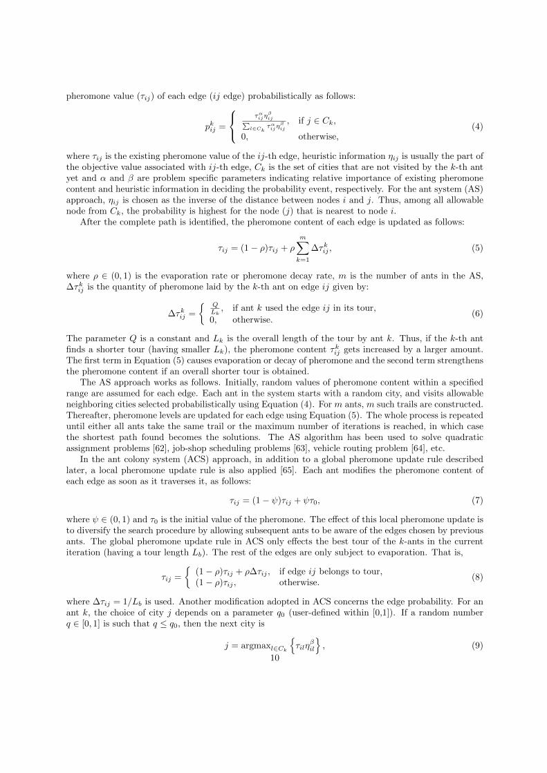
pheromone value (τij) of each edge (ij edge) probabilistically as follows:

pkij =

ταijη

βij∑

l∈Ckταijη

βij

, if j ∈ Ck,

0, otherwise,(4)

where τij is the existing pheromone value of the ij-th edge, heuristic information ηij is usually the part ofthe objective value associated with ij-th edge, Ck is the set of cities that are not visited by the k-th antyet and α and β are problem specific parameters indicating relative importance of existing pheromonecontent and heuristic information in deciding the probability event, respectively. For the ant system (AS)approach, ηij is chosen as the inverse of the distance between nodes i and j. Thus, among all allowablenode from Ck, the probability is highest for the node (j) that is nearest to node i.

After the complete path is identified, the pheromone content of each edge is updated as follows:

τij = (1− ρ)τij + ρ

m∑k=1

∆τkij , (5)

where ρ ∈ (0, 1) is the evaporation rate or pheromone decay rate, m is the number of ants in the AS,∆τkij is the quantity of pheromone laid by the k-th ant on edge ij given by:

∆τkij =

{QLk, if ant k used the edge ij in its tour,

0, otherwise.(6)

The parameter Q is a constant and Lk is the overall length of the tour by ant k. Thus, if the k-th antfinds a shorter tour (having smaller Lk), the pheromone content τkij gets increased by a larger amount.The first term in Equation (5) causes evaporation or decay of pheromone and the second term strengthensthe pheromone content if an overall shorter tour is obtained.

The AS approach works as follows. Initially, random values of pheromone content within a specifiedrange are assumed for each edge. Each ant in the system starts with a random city, and visits allowableneighboring cities selected probabilistically using Equation (4). For m ants, m such trails are constructed.Thereafter, pheromone levels are updated for each edge using Equation (5). The whole process is repeateduntil either all ants take the same trail or the maximum number of iterations is reached, in which casethe shortest path found becomes the solutions. The AS algorithm has been used to solve quadraticassignment problems [62], job-shop scheduling problems [63], vehicle routing problem [64], etc.

In the ant colony system (ACS) approach, in addition to a global pheromone update rule describedlater, a local pheromone update rule is also applied [65]. Each ant modifies the pheromone content ofeach edge as soon as it traverses it, as follows:

τij = (1− ψ)τij + ψτ0, (7)

where ψ ∈ (0, 1) and τ0 is the initial value of the pheromone. The effect of this local pheromone update isto diversify the search procedure by allowing subsequent ants to be aware of the edges chosen by previousants. The global pheromone update rule in ACS only effects the best tour of the k-ants in the currentiteration (having a tour length Lb). The rest of the edges are only subject to evaporation. That is,

τij =

{(1− ρ)τij + ρ∆τij , if edge ij belongs to tour,(1− ρ)τij , otherwise.

(8)

where ∆τij = 1/Lb is used. Another modification adopted in ACS concerns the edge probability. For anant k, the choice of city j depends on a parameter q0 (user-defined within [0,1]). If a random numberq ∈ [0, 1] is such that q ≤ q0, then the next city is

j = argmaxl∈Ck

{τilη

βil

}, (9)

10

Algorithm 2 Ant Colony Optimization

Require: m, n, α, β, ρ, ψ, q0, τ0, Q1: Set iteration counter t = 02: Set best route length Lbest to ∞3: if AS is desired then4: Randomly initialize edge pheromone levels within a range5: end if6: if ACS is desired then7: Initialize all edge pheromone levels to τ08: end if9: repeat

10: for k = 1 to m do11: Randomly place ant k at one of the n cities12: repeat13: if ACS is desired and rand(0, 1) ≤ q0 then14: Choose next city to be visited using Equation (9)15: else16: Choose next city to be visited using Equation (4)17: end if18: if ACS is desired then19: Update current edge using local pheromone update rule in Equation (7)20: end if21: until unvisited cities exist22: Find best route having length Lb23: if ACS is desired then24: Update edges of best route using global pheromone update rule in Equation (8)25: end if26: if AS is desired then27: for all edges do28: Update current edge using pheromone update rule in Equation (5)29: end for30: end if31: end for32: if Lb < Lbest then33: Lbest = Lb34: end if35: t← t+ 136: until TP is satisfied37: Declare route length Lbest as near-optimal solution

11

otherwise Equation (4) is used.Both AS and ACS can be represented by the pseudocode in Algorithm 2.ACO for solving continuous optimization problems is not straightforward, yet attempts have been

made [66, 67, 68] to change the pheromone trail model, which is by definition a discrete probabilitydistribution, to a continuous probability density function. Moreover, presently there is no clear under-standing of which algorithms may be called ant based. Stigmergy optimization is the generic name givento algorithms that use multiple agents exchanging information in an indirect manner [69].

4. Artificial Bee Colony Optimization (ABCO)

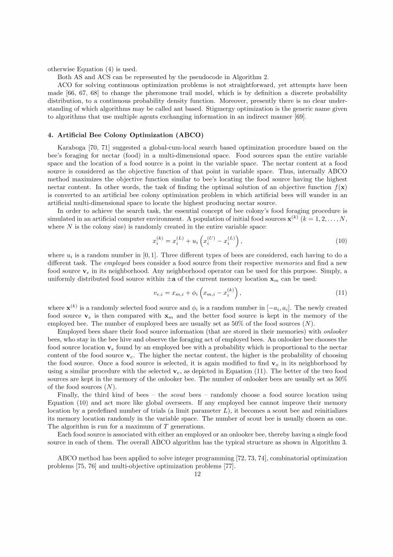
Karaboga [70, 71] suggested a global-cum-local search based optimization procedure based on thebee’s foraging for nectar (food) in a multi-dimensional space. Food sources span the entire variablespace and the location of a food source is a point in the variable space. The nectar content at a foodsource is considered as the objective function of that point in variable space. Thus, internally ABCOmethod maximizes the objective function similar to bee’s locating the food source having the highestnectar content. In other words, the task of finding the optimal solution of an objective function f(x)is converted to an artificial bee colony optimization problem in which artificial bees will wander in anartificial multi-dimensional space to locate the highest producing nectar source.

In order to achieve the search task, the essential concept of bee colony’s food foraging procedure issimulated in an artificial computer environment. A population of initial food sources x(k) (k = 1, 2, . . . , N ,where N is the colony size) is randomly created in the entire variable space:

x(k)i = x

(L)i + ui

(x(U)i − x(L)i

), (10)

where ui is a random number in [0, 1]. Three different types of bees are considered, each having to do adifferent task. The employed bees consider a food source from their respective memories and find a newfood source ve in its neighborhood. Any neighborhood operator can be used for this purpose. Simply, auniformly distributed food source within ±a of the current memory location xm can be used:

ve,i = xm,i + φi

(xm,i − x(k)i

), (11)

where x(k) is a randomly selected food source and φi is a random number in [−ai, ai]. The newly createdfood source ve is then compared with xm and the better food source is kept in the memory of theemployed bee. The number of employed bees are usually set as 50% of the food sources (N).

Employed bees share their food source information (that are stored in their memories) with onlookerbees, who stay in the bee hive and observe the foraging act of employed bees. An onlooker bee chooses thefood source location ve found by an employed bee with a probability which is proportional to the nectarcontent of the food source ve. The higher the nectar content, the higher is the probability of choosingthe food source. Once a food source is selected, it is again modified to find vo in its neighborhood byusing a similar procedure with the selected ve, as depicted in Equation (11). The better of the two foodsources are kept in the memory of the onlooker bee. The number of onlooker bees are usually set as 50%of the food sources (N).

Finally, the third kind of bees – the scout bees – randomly choose a food source location usingEquation (10) and act more like global overseers. If any employed bee cannot improve their memorylocation by a predefined number of trials (a limit parameter L), it becomes a scout bee and reinitializesits memory location randomly in the variable space. The number of scout bee is usually chosen as one.The algorithm is run for a maximum of T generations.

Each food source is associated with either an employed or an onlooker bee, thereby having a single foodsource in each of them. The overall ABCO algorithm has the typical structure as shown in Algorithm 3.

ABCO method has been applied to solve integer programming [72, 73, 74], combinatorial optimizationproblems [75, 76] and multi-objective optimization problems [77].

12

Algorithm 3 Artificial Bee Colony Optimization Algorithm

Require: N , L1: Set iteration counter t = 02: Initialize N/2 employer bees (solutions) to N/2 food sources using Equation (10)3: repeat4: Find nectar content at employer bee locations (i.e. evaluate solutions xm)5: Move each employer bee to a new food source in its neighborhood using Equation (11)6: Find nectar content at new employer bee locations (i.e. evaluate solutions ve)7: Record employer bees that return to xm due to lower nectar content at ve8: Recruit N/2 onlooker bees to employer bee locations with probabilities proportional to their nectar

content9: Move each onlooker bee to a new food source in its neighborhood (similar to Equation (11))

10: Find nectar content at new onlooker bee locations (i.e. evaluate solutions vo)11: Move each employer bee to the best location found by onlooker bees assigned to it12: Record the best food source among all xm, ve and vo13: Convert employer bees that cannot find better food sources in L trials into scout bees14: Initialize scout bees, if any, using Equation (10)15: t← t+ 116: until TP is satisfied17: Declare the best food source (near-optimal solution)

5. Artificial Immune System (AIS)

Immune systems in biological organisms protect living cells from an attack from foreign bodies. Whenattacked by antigens, different antibodies are produced to defend the organism. In a macro sense, thenatural immune system works as follows. Antibodies that are efficient in fighting antigens are cloned,hyper-mutated and more such antibodies are produced to block the action of antigens. Once successful,the organism learns to create efficient antibodies. Thus, later if similar antigens attack, the organismcan quickly produce the right antibodies to mitigate their effect. The process of developing efficientantibodies can be simulated to solve optimization problems, in which antibodies can represent decisionvariables and the process of cloning, hyper-mutation and selection can be thought as a search processfor finding optimal antibodies that tend to match or reach the extremum values of antigens representingobjectives. There are mainly two different ways such an immunization task is simulated, which we discussnext.

5.1. Clonal Selection Algorithm

Proposed by Burnet [78] in 1959, the clonal selection procedure works with the concept of cloningand affinity maturation. When exposed to antigens, B-cells (so called because they are produced in thebone marrow) that best bind with the attacking antigens get emphasized through cloning. The abilityof binding depends on how well the paratope of an antibody matches with the epitope of an antigen.The closer the match, the stronger is the affinity of binding. In the context of a minimization problem,the following analogy can drive the search towards the minimum. The smaller the value of the objectivefunction for an antibody representing a solution, the higher can be the affinity level. The cloned antibodiescan then undergo hyper-mutation according to an inverse relationship to their affinity level. Receptorediting and introduction of random antibodies can also be implemented to maintain a diverse set ofantibodies (solutions) in the population. These operations sustain the affinity maturation process.

The clonal selection algorithm CLONALG [79, 80] works as follows. First, a population of N an-tibodies is created at random. An antibody can be a vector of real, discrete or Boolean variables, orit can be a permutation or a combination of the above, depending on the optimization problem beingsolved. At every iteration, a small fraction (say, n out of N) of antibodies is selected from the population

13

based on their affinity level. These high-performing antibodies are then cloned and then hyper-mutatedto construct Nc new antibodies. The cloning is directly proportional to the ranking of the antibodies interms of their affinity level. The antibody with the highest affinity level in a population has the largestpool of clones. Each clone antibody is then mutated with a probability that is higher for antibodieshaving a lower affinity level. This allows a larger mutated change to occur in antibodies that are worse interms of antigen affinity (or worse in objective values). Since a large emphasis of affinity level is placedon the creation mechanism of new antibodies, some randomly created antibodies are also added to thepopulation to maintain adequate diversity. After all newly created antibodies are evaluated to obtaintheir affinity level, R% worst antibodies are replaced by the best newly created antibodies. This processcontinues till a pre-specified termination criterion is satisfied. Algorithm 4 shows the basic steps.

Algorithm 4 Artificial Immune Systems - Clonal Selection Algorithm

Require: N , n, Nc, R1: Set iteration counter t = 02: Randomly initialize N antibodies to form St3: repeat4: Evaluate affinity (fitness) of all antibodies in St5: Select n antibodies with highest affinities to form Pt6: Clone the n antibodies in proportion to their affinities to generate Nc antibodies7: Hyper-mutate the Nc antibodies to form Ct8: Evaluate affinity of all antibodies in Ct9: Replace R% worst antibodies in St with the best antibodies from Ct

10: Add new random antibodies to St11: t← t+ 112: until TP is satisfied13: Declare population best as near-optimal solution

On careful observation, the clonal selection algorithm described above is similar to a genetic algorithm(GA), except that no recombination-like operator is used in the clonal selection algorithm. The clonalselection algorithm is a population-based optimization algorithm that uses overlapping populations andheavily relies on a mutation operator whose strength directly relates to the value of objective function ofthe solution being mutated.

5.2. Immune Network Algorithm

A natural immune system, although becomes active when attacked by external antigen, sometimes canwork against its own cells, thus stimulating, activating or suppressing each other. To reduce the chance ofevents, the clonal selection algorithm has been modified to recognize antibodies (solutions) that are similarto one another in an evolving antibody population. Once identified, similar antibodies (in terms of adistance measure) are eliminated from the population through clonal suppression. Moreover, antibodieshaving very small affinity level towards attacking antigens (meaning worse than a threshold objectivefunction value) are also eliminated from the population. In the artificial immune network (aiNET [81])algorithm, a given number of affinity clones are selected to form an immune network. These clones arethought to form a clonal memory. The clonal suppression operation is performed on the antibodies of theclonal memory set. The aiNET algorithm works as follows. A population of N antibodies are created atrandom. A set of n antibodies are selected using their affinity level. Thereafter, each is cloned based ontheir affinity level in a manner similar to that in the clonal selection algorithm. Each clone is then hyper-mutated as before and are saved within a clonal memory set (M). After evaluation, all memory clonesthat have objective value worse than a given threshold ε are eliminated. Antibodies that are similar (e.g.solutions clustered together) to each other are also eliminated through the clonal suppression processusing a suppression threshold σs. A few random antibodies are injected in the antibody population as

14

before, and the process is continued till a termination criterion is satisfied. The pseudocode for a typicalimmune network algorithm is shown in Algorithm 5.

Algorithm 5 Artificial Immune Systems - Immune Network Algorithm

Require: N , n, Nc, ε, σs, R1: Set iteration counter t = 02: Set clonal memory set M = Φ3: Randomly initialize N antibodies to form St4: repeat5: Evaluate affinity (fitness) of all antibodies in St6: Select n antibodies with highest affinities to form Pt7: Clone the n antibodies in proportion to their affinities to generate Nc antibodies8: Mutate the Nc antibodies in inverse-proportion to their affinities to form Ct9: Evaluate affinity of all antibodies in Ct

10: M = M ∪ Ct11: Eliminate memory clones from M with affinities < ε12: Calculate similarity measure s for all clonal pairs in M13: Eliminate memory clones from M with s < σs14: Replace R% worst antibodies in St with the best antibodies from M15: Add new random antibodies to St16: t← t+ 117: until TP is satisfied18: Declare the best antibody in M as near-optimal solution

In the context of optimization, artificial immune system (AIS) algorithms are found to be usefulin following problems. Dynamic optimization problems in which the optimum changes with time is apotential application domain [82] simply because AIS is capable of quickly discovering a previously-foundoptimum if it appears again at a later time. The immune network algorithm removes similar solutions fromthe population, thereby allowing multiple disparate solutions to co-exist in the population. This allowedAIS algorithms to solve multi-modal optimization problems [83] in which the goal is to find multiplelocal or global optima in a single run. AIS methods have also been successfully used for solving travelingsalesman problems [84]. Several hybrid AIS methods coupled with other evolutionary approaches areproposed [85]. AIS has also been hybridized with ant colony optimization (ACO) algorithms [86]. Moredetails can be found elsewhere [87].

6. Differential Evolution (DE)

Differential evolution was proposed by Storn and Price [88] as a robust and easily parallelizablealternative to global optimization algorithms. DE borrows the idea of self-organizing from Nelder-Mead’ssimplex search algorithm [89], which is also a popular heuristic search method. Like other population-based metaheuristics, DE also starts with a population of randomly initialized solution vectors. However,instead of using variation operators with predetermined probability distributions, DE uses the differencevector of two randomly chosen members to modify an existing solution in the population. The differencevector is weighted with a user-defined parameter F > 0 and to a third (and different) randomly chosenvector as shown below:

vi,t+1 = xr1,t + F · (xr2,t − xr3,t). (12)

At each generation t, it is ensured that r1, r2 and r3 are different from each other and also from i. Theresultant vector vi is called a mutant vector of xi. F remains constant with generations and is fixed in[0, 2] (recommended [0.4, 1] [90]).

15

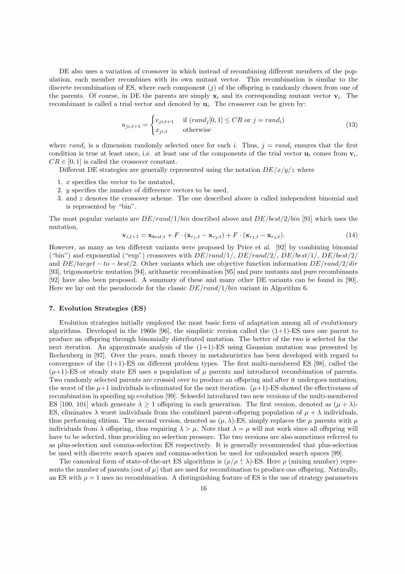
DE also uses a variation of crossover in which instead of recombining different members of the pop-ulation, each member recombines with its own mutant vector. This recombination is similar to thediscrete recombination of ES, where each component (j) of the offspring is randomly chosen from one ofthe parents. Of course, in DE the parents are simply xi and its corresponding mutant vector vi. Therecombinant is called a trial vector and denoted by ui. The crossover can be given by:

uji,t+1 =

{vji,t+1 if (randj [0, 1] ≤ CR or j = randi)

xji,t otherwise(13)

where randi is a dimension randomly selected once for each i. Thus, j = randi ensures that the firstcondition is true at least once, i.e. at least one of the components of the trial vector ui comes from vi.CR ∈ [0, 1] is called the crossover constant.

Different DE strategies are generally represented using the notation DE/x/y/z where

1. x specifies the vector to be mutated,2. y specifies the number of difference vectors to be used,3. and z denotes the crossover scheme. The one described above is called independent binomial and

is represented by “bin”.

The most popular variants are DE/rand/1/bin described above and DE/best/2/bin [91] which uses themutation,

vi,t+1 = xbest,t + F · (xr1,t − xr2,t) + F · (xr3,t − xr4,t). (14)

However, as many as ten different variants were proposed by Price et al. [92] by combining binomial(“bin”) and exponential (“exp”) crossovers with DE/rand/1/, DE/rand/2/, DE/best/1/, DE/best/2/and DE/target− to− best/2. Other variants which use objective function information DE/rand/2/dir[93], trigonometric mutation [94], arithmetic recombination [95] and pure mutants and pure recombinants[92] have also been proposed. A summary of these and many other DE variants can be found in [90].Here we lay out the pseudocode for the classic DE/rand/1/bin variant in Algorithm 6.

7. Evolution Strategies (ES)

Evolution strategies initially employed the most basic form of adaptation among all of evolutionaryalgorithms. Developed in the 1960s [96], the simplistic version called the (1+1)-ES uses one parent toproduce an offspring through binomially distributed mutation. The better of the two is selected for thenext iteration. An approximate analysis of the (1+1)-ES using Gaussian mutation was presented byRechenberg in [97]. Over the years, much theory in metaheuristics has been developed with regard toconvergence of the (1+1)-ES on different problem types. The first multi-membered ES [98], called the(µ+1)-ES or steady state ES uses a population of µ parents and introduced recombination of parents.Two randomly selected parents are crossed over to produce an offspring and after it undergoes mutation,the worst of the µ+1 individuals is eliminated for the next iteration. (µ+1)-ES showed the effectiveness ofrecombination in speeding up evolution [99]. Schwefel introduced two new versions of the multi-memberedES [100, 101] which generate λ ≥ 1 offspring in each generation. The first version, denoted as (µ + λ)-ES, eliminates λ worst individuals from the combined parent-offspring population of µ + λ individuals,thus performing elitism. The second version, denoted as (µ, λ)-ES, simply replaces the µ parents with µindividuals from λ offspring, thus requiring λ > µ. Note that λ = µ will not work since all offspring willhave to be selected, thus providing no selection pressure. The two versions are also sometimes referred toas plus-selection and comma-selection ES respectively. It is generally recommended that plus-selectionbe used with discrete search spaces and comma-selection be used for unbounded search spaces [99].

The canonical form of state-of-the-art ES algorithms is (µ/ρ +, λ)-ES. Here ρ (mixing number) repre-sents the number of parents (out of µ) that are used for recombination to produce one offspring. Naturally,an ES with ρ = 1 uses no recombination. A distinguishing feature of ES is the use of strategy parameters

16

Algorithm 6 Differential Evolution

Require: N , F , CR1: Set iteration counter t = 02: Randomly initialize N population members to form St3: repeat4: Evaluate fitness of all members in St5: for i = 1 to N do6: Generate random integer randi between 1 and search space dimension D7: for j = 1 to D do8: Generate random number randj ∈ [0, 1]9: if randj ≤ CR or j = randi then

10: uji,t+1 = vji,t+1 = xjr1,t + F · (xjr2,t − xjr3,t)11: else12: uji,t+1 = xji,t13: end if14: end for15: Evaluate trial vector ui,t+1

16: if f(ui,t+1) ≤ f(xi,t) then17: Replace xi,t with ui,t+1

18: end if19: end for20: t← t+ 121: until TP is satisfied22: Declare population best as near-optimal solution

s that are unique for each individual. These so called endogenous strategy parameters can evolve withgenerations. Most self-adaptive ES use these evolvable parameters to tune the mutation strength. Thesestrategy parameters can also be recombined and mutated like the solution vectors. On the other hand,exogenous strategy parameters µ, ρ and λ remain unchanged with generations. Algorithm 7 shows thegeneric ES procedure.

Recombination of the ρmembers can either be discrete (dominant) or intermediate. In the former, eachdimension of the offspring is randomly chosen from the corresponding dimension of the parents, whereas inthe latter, all dimensions of the offspring are arithmetically averaged values of corresponding dimensionsover all parents. For strategy parameters intermediate (µ/µ) recombination has been recommended in[99] and [102] to avoid over-adaptation or large fluctuations.

Traditionally, ES variants have only used mutation as the variation operator. As a result, manystudies exist which discuss, both theoretically [103, 104] and empirically, the effect of mutation strengthon the convergence of ES and the self-adaptation of strategy parameters in mutation operators [105],most notably that of the standard deviation in Gaussian distribution mutation. Self-adaptive ES haveemerged to be one of the most competitive metaheuristic methods in recent time. We describe themnext.

7.1. Self-adaptive ES

A self-adaptive ES is one in which the endogenous strategy parameters (whether belonging to recom-bination or mutation) can tune (adapt) themselves based on the current distribution of solutions in thesearch space. The basic idea is to try bigger steps if past steps have been successful and smaller stepswhen they have been unsuccessful. However, as mentioned before, most self-adaptive ES are concernedwith the strategy parameter of mutation and this is what we discuss here. Discussions on other strategyparameters can be found in [106].

17

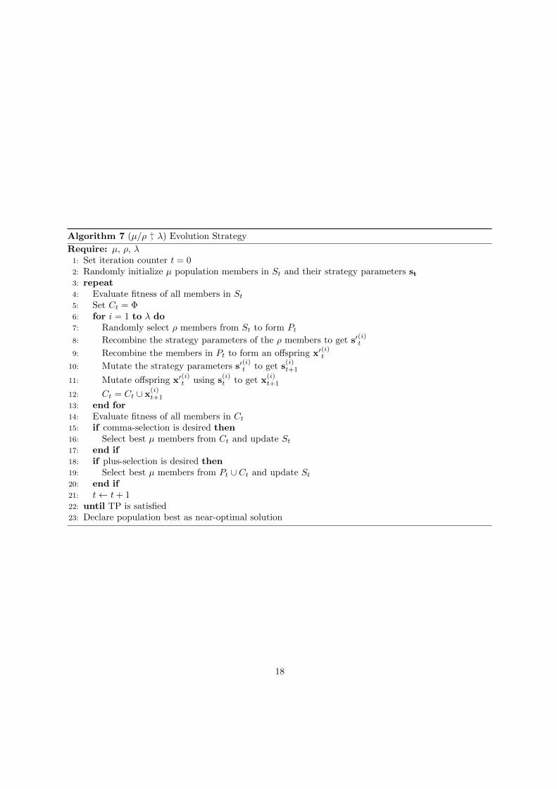
Algorithm 7 (µ/ρ +, λ) Evolution Strategy

Require: µ, ρ, λ1: Set iteration counter t = 02: Randomly initialize µ population members in St and their strategy parameters st3: repeat4: Evaluate fitness of all members in St5: Set Ct = Φ6: for i = 1 to λ do7: Randomly select ρ members from St to form Pt8: Recombine the strategy parameters of the ρ members to get s′

(i)t

9: Recombine the members in Pt to form an offspring x′(i)t

10: Mutate the strategy parameters s′(i)t to get s

(i)t+1

11: Mutate offspring x′(i)t using s

(i)t to get x

(i)t+1

12: Ct = Ct ∪ x(i)t+1

13: end for14: Evaluate fitness of all members in Ct15: if comma-selection is desired then16: Select best µ members from Ct and update St17: end if18: if plus-selection is desired then19: Select best µ members from Pt ∪ Ct and update St20: end if21: t← t+ 122: until TP is satisfied23: Declare population best as near-optimal solution

18

For unconstrained real-valued search spaces, the maximum entropy principle says that the variationoperator should use a normal distribution so as to not introduce any bias during exploration [99]. Themutation operation on a solution (or ‘recombinant’ if crossover is used) x′ is therefore given by,

x = x′ + σN(0, I) = σN(x′, I), (15)

where σ (= s in Algorithm 7) is the only strategy parameter and N(0, I) is a zero-mean unit-variancenormally distributed random vector. Thus, each component i of the mutant x obeys the following densityfunction:

prob(x′i) =1√2πσ

exp

(− (x′i − xi)2

2σ2

). (16)

The mutation strength σ is thus the standard deviation of the mutant distribution, which implies σ > 0.It is also sometimes called the step-size when referring to Equation (15). Note that for σ being anendogenous strategy parameter, also undergoes recombination and mutation. As discussed above, re-combination of strategy parameters is mainly intended to reduce fluctuations in values and thereforeintermediate recombination (arithmetic averaging of standard deviations of parents) is often used. Mu-tation of the mutation strength is multiplicative since an additive mutation (like that in Equation (15))cannot guarantee σ > 0. For a strategy parameter value (or ‘recombinant’ if crossover is used) σ′, the‘log-normal’ mutation operator [100] is given by,

σ = σ′ exp(τN(0, 1)), (17)

where τ is called the learning parameter and is proportional to 1/√N (usually τ = 1/

√2N), N being the

search space dimension. A self-adaptive ES using Equation (17) in Step 10 and Equation (15) in Step 11of Algorithm 7 is called (µ/ρ +, λ)-σSA-ES in literature.

When multiple strategy parameters are used i.e. when s = σ, Equation (15) becomes,

x = x′ + diag(σ1, σ2, . . . , σN )N(0, I). (18)

Here, diag() is a diagonal matrix with elements σ1, σ2, etc. representing the standard deviations formutation along different dimensions. This allows for axes-parallel ellipsoidal mutant distributions. Self-adaptation in this case is given by the extended log-normal rule [101],

σ = exp(τ0N(0, 1))

σ′1 exp(τN1(0, 1))σ′2 exp(τN1(0, 1))

...σ′N exp(τNN (0, 1))

. (19)

τ0 acts as a global learning parameter and τ acts on coordinate-wise on each normal distribution Ni(0, 1).

Recommended values for them are τ0 ∝ 1/√

2N and τ ∝ 1/√

2√N .

7.2. Covariance Matrix Adaptation-ES (CMA-ES)

CMA-ES [107] and its variants [108, 109, 110] represent the state-of-the-art of self-adaptive ES algo-rithms for continuous search space optimization. The main difference in CMA-ES from self-adaptive ESis that it uses a generic multivariate normal distribution for mutation which is given by

x = xm + σN(0,C) = σN(xm,C), (20)

where C is the covariance matrix which enables arbitrarily rotated ellipsoidal mutant distributions. Bycontrast, the mutant distribution obtained from Equation (15) is always spherical while that obtainedfrom Equation (18) is always an axes-parallel ellipsoid.

19

Another important difference is that while self-adaptive ES starts with a population of randomlyinitialized solutions, CMA-ES starts with a random population mean xm and generates λ offspringusing Equation (20). C is initialized to an identity matrix so that the initial offspring distribution isspherical. After evaluating the λ offspring, µ best solutions are selected and recombined using a weightedintermediate recombination given by,

x′m =

µ∑i=1

wixi:λ (21)

to produce a single recombinant representing the new population mean x′m. The best offspring getsthe largest weight and the µ-th best offspring gets the least weight. Additionally, the weights satisfyw1 ≥ w2 ≥ w3 . . . ≥ wµ > 0,

∑wi = 1 and µw = 1/

∑w2i ≈ λ/4. Due to this selection scheme CMA-ES

is also known as (µ/µw, λ)-CMA-ES.Rewriting x′m as below, we can define y and yw.

x′m = xm + σ

µ∑i=1

wi

(xi:λ − xm

σ

)= xm + σ

µ∑i=1

wiyi:λ = xm + σyw. (22)

Next the step-size σ and the covariance matrix C are updated using the following formulae:

p′σ = (1− cσ)pσ +√

1− (1− cσ)2√µw√

C−1yw, (23)

p′c = (1− cc)pc + 1(||p′σ||<1.5

√N)

√1− (1− cc)2

õwyw, (24)

C′ = (1− c1 − cµ)C + c1p′cp′cT

+ cµ

µ∑i=1

wiyi:λyTi:λ (25)

σ′ = σ exp

(cσdσ

(||p′σ||

E [||N(0, I)||]− 1

))(26)

Here, the values cc, cσ ≈ 4/N , c1 ≈ 2/N2, cµ ≈ µw/N2 and dσ = 1 +

õw/N are often used.

1(||p′σ||<1.5

√N) represents an indicator function which is equal to one when its subscript is true, else

it is equal to zero. E [||N(0, I)||] represents the expected norm of a normally distributed random vector.pc and pσ are called the evolution paths of the covariance matrix and step-size, respectively. Initializa-tions C = I and pc,pσ = 0 are used at the start of the algorithm. The above updates ensure that C issymmetric and positive semi-definite, as required for covariance matrices, at each iteration. The deriva-tion of the above equations is mathematically involved and readers are referred to the original CMA-ESpaper [111] and [107, 108, 109] for details and explanation of parameter settings. The pseudocode forCMA-ES is shown in Algorithm 8 for an N dimensional search space.

8. Evolutionary Programming (EP)

Evolutionary programming together with genetic algorithms and evolutionary strategies are the ear-liest paradigms of evolutionary algorithms. It was developed by Lawrence J. Fogel [112] in 1960. Themain difference from GA and ES is that EP does not use a recombination or crossover operator. Thereason for this is that EP was originally designed as an abstraction of evolution at the macro level ofspecies, rather than at the genetic level. Thus instead of individuals of a population which can mate andreproduce, EP considers each individual as a reproducing population and the aim is to mimic the linkagebetween parent and its offspring [113, 114].

EP, like any other evolutionary algorithm, starts with a population of µ randomly initialized popu-lation members. Each member undergoes mutation to produce an offspring. Different EP variants usedifferent mutation schemes. The original EP [112] described the evolution of finite state machines usinguniform random mutations on discrete variables. David B. Fogel [115] introduced normally distributed

20

Algorithm 8 (µ/µw, λ) Covariance Matrix Adaptation - Evolution Strategy

Require: λ, µ (= λ/2 typically)1: Set recombination weights wi ∀ i = 1, . . . , µ, Recommended wi = ln(λ+1

2 )− ln(i)2: Renormalize weights such that

∑wi = 1

3: Set µw = 1/∑w2i , cc, cσ ≈ 4/N , c1 ≈ 2/N2, cµ ≈ µw/N2 and dσ = 1 +

õw/N

4: Set iteration counter t = 05: Set Ct = I, pct,pσt = 06: Randomly initialize mean point xmt and step-size σt > 0, Recommended σt = 0.37: repeat8: Generate λ offspring from xmt using Equation (20) and form Ct9: Evaluate fitness of f(x) all members in Ct

10: Sort members of Ct according to their fitness11: Choose µ best individuals from Ct and form Pt12: Generate updated mean x′m from Pt using Equation (21)13: Generate updated step-size evolution path p′σ using Equation (23)14: Generate updated covariance evolution path p′c using Equation (24)15: Generate updated covariance matrix C′ using Equation (25)16: Generate updated step-size σ′ using Equation (26)17: xmt+1 = x′m18: pct+1 = p′c and pσt+1 = p′σ19: Ct+1 = C′ and σt+1 = σ′

20: t← t+ 121: until TP is satisfied22: Declare current xm as near-optimal solution

mutations for real-valued variables where the standard deviation for an individual’s mutation is a functionof its fitness value, i.e.,

x = x′ + σN(0, I),

σ =√G(f(x′), κ),

(27)

where G is a fitness function that scales the objective function values to positive values and also sometimesuses random alteration κ. Fogel later introduced meta-EP [116] that uses self-adaptation in a mannersomewhat similar to that used in ES for multiple strategy parameters, i.e.,

x = x′ + diag(σ1, σ2, . . . , σN )N(0, I),

σ2i = σ′i

2+√ζσ′iNi(0, 1) ∀i = 1, . . . , N.

(28)

where ζ is an exogenous parameter. Meta-EP self-adaptation differs with respect to the underlyingstochastic process. Unlike the log-normal mutation in ES which guarantees positiveness of σ, negativevariances can occur in EP. When this happens σi =

√εc > 0 is used. Later versions of EP [117] use ES’s

self-adaptation as shown in Equation (19). Fogel also proposed Rmeta-EP [118] for N = 2 dimensionswhich uses correlation coefficients similar to CMA-ES. However, its generalization for N > 2 is notobvious [119].

Once µ offspring are created using mutation, EP uses a kind of (µ+ µ) stochastic selection. For eachsolution in the combined parent-offspring population of size 2µ, q other solutions are randomly selectedfrom the population. The score w ∈ {0, . . . , q} of each solution is the number of those q solutions thatare worser than it, i.e.,

wi =

q∑j=1

{1 if f(xi) ≤ f(xj:2µ)

0 otherwise∀i = {1, . . . , 2µ}. (29)

21

Thereafter, µ individuals with the best scores are chosen for the next iteration. Note that this selectionstrategy becomes more and more deterministic, approaching that in ES, as q increases. A little thoughtalso reveals that the selection is elitist. The pseudocode for EP is shown in Algorithm 91.

Algorithm 9 Evolutionary Programming

Require: µ, q, Mutation parameters ({G, κ} or {ζ, εc} or {τ0, τ})1: Set iteration counter t = 02: Randomly initialize µ population members and σi ∀i = {1, . . . , N} (if used) to form St3: repeat4: Evaluate fitness f(x′) of all members in Pt = St5: if standard EP is used then6: Mutate individuals in Pt using Equation (27) to form Ct7: end if8: if meta-EP is used then9: Mutate individuals in Pt using Equation (28) to form Ct

10: end if11: if EP with ES’s self-adaptation is used then12: Mutate individuals in Pt using Equations (18) and Equation (19) to form Ct13: end if14: for i = 1 to 2µ do15: Select xi from Pt ∪ Ct16: Set wi = 017: Select q individuals randomly from Pt ∪ Ct to form Qt18: for j = 1 to q do19: Select xj from Qt20: if f(xi) ≤ f(xj) then21: wi ← wi + 122: end if23: end for24: end for25: Sort members of Pt ∪ Ct according to their scores w26: Replace St with µ best score members of Pt ∪ Ct27: t← t+ 128: until TP is satisfied29: Declare population best as near-optimal solution

9. Genetic Algorithms (GA)

Genetic algorithms are among the most popular of metaheuristic techniques. Introduced in 1975through the seminal work of John Holland [120], its framework for search and optimization, now popu-larly known as Binary-coded Genetic Algorithm (BGA), was developed by Goldberg [121]. In a BGA,solutions are represented using binary-bit strings which are iteratively modified through recombinationand random bit-flips, much like the evolution of genes in nature, which also undergo natural selection,genetic crossovers and mutations. The ease of implementation and generality of BGA made it a popularchoice of metaheuristic in the following years. However, inherent problems were also identified along the

1Note that this section used ‘primed’ symbols, x′ and σ′i, even though they are not recombinants, in order to facilitatecomparison with ES

22

way, most notably Hamming cliffs, unnecessary search space discretization and ineffective schema prop-agation in case of more than two virtual alphabets. These paved the way for Real-parameter GeneticAlgorithm (RGA). In an RGA, a solution is directly represented as a vector of real-parameter decisionvariables. Starting with a population of such solutions (usually randomly created), a set of genetic oper-ations (such as selection, recombination, mutation, and elite-preservation) are performed to create a newpopulation in an iterative manner. Clearly, the selection plan (SP) must implement the selection opera-tor of RGAs, the generational plan (GP) must implement all variation operators (such as recombinationand mutation operators), and the update plan (UP) must implement any elite-preservation operator.Although most RGAs differ from each other mainly in terms of their recombination and mutation op-erators, they mostly follow one of the two algorithmic models discussed later. First, we shall discusssome commonly-used GA operators which can be explained easily with the help of the five plans outlinedbefore.

Among GA’s many selection operators, the proportionate selection scheme (or roulette wheel selec-tion), the ranking scheme and the tournament selection operators are most popular. With the proposedmetaheuristic algorithm, these operators must be represented in the selection plan. For example, theproportionate selection operator can be implemented by choosing the i-th solution for its inclusion to Ptwith a probability fi/

∑i fi. This probability distribution around St is used to choose µ members of Pt.

The ranking selection operator uses sorted ranks instead of actual function values to obtain probabilitiesof solutions to be selected. The tournament selection operator with a size s can be implemented by usinga SP in which s solutions are chosen and the best is placed in Pt. The above procedure needs to berepeated µ times to create the parent population Pt.

Traditionally, BGAs have used variants of point crossover and bit-flip mutation operators. RGAs,on the other hand, use blending operators [122] for recombination of solutions. BLX-α [123], simulatedbinary crossover (SBX) [124] and fuzzy recombination [125] are often used in literature. SBX emulatesa single-point binary crossover in that the average decoded values of parents and their offspring areequal. The offspring are thus symmetrically located with respect to the parents. Moreover, it usesa polynomial probability distribution function which ensures that the probability of creating offspringcloser to the parents is greater. The distribution can also be easily modified when the variables arebounded [124]. Mutation operators for RGAs such as random mutation [126], uniform mutation [127],non-uniform mutation [126], normally distributed mutation [128] and polynomial mutation [129] havealso been developed.

Elite preservation in a GA is an important task [130]. This is enforced by allowing best of parent andoffspring populations to be propagated in two consecutive iterations. The update plan of the proposedalgorithm-generator achieves elite preservation in a simple way. As long as the previous population Stor the chosen parent population Pt is included in the update plan for choosing better solutions, elitepreservation is guaranteed. Most GAs achieve this by choosing the best µ solutions from a combinedpopulation of Pt and Ct.

A niche-preservation operator is often used to maintain a diverse set of solutions in the population.Only the selection plan gets affected for implementing a niche-preservation operator. While choosingthe parent population Pt, care should be taken to lower the selection probability of population-bestsolutions in Pt. Solutions with a wider diversity in their decision variables must be given priorities. Thestandard sharing function approach [131], clearing approaches [132], and others can be designed using anappropriate selection plan.

A mating restriction operator, on the other hand, is used to reduce the chance of creating lethalsolutions arising from mating of two dissimilar yet good solutions. This requires a SP in which theprocedures of choosing of each of the µ parents become dependent on each other. Once the first parentis chosen, the procedure of choosing other parents must consider a similarity measure with respect to thefirst parent.

23

9.1. Generational Versus Steady-State GAsEvolutionary algorithms, particularly genetic algorithms, are often used with a generational or with a

steady-state concept. In the case of former, a complete population of λ solutions are first created beforemaking any further decision. The proposed metaheuristic algorithm can be used to develop a generationalGA by repeatedly using the SP-GP plans to create λ new offspring solutions. Thereafter, the replacementplan simply chooses the whole parent population to be replaced, or Rt = St (and ρ = µ). With an elite-preservation operator, the update plan chooses the best µ solutions from the combined population St∪Ct.In a GA without elitism, the update plan only chooses the complete offspring population Ct.

On the other extreme, a steady-state GA can be designed by using a complete SP-GP-RP-UP cyclefor creating and replacing only one solution (λ = r = 1) in each iteration. It is interesting to note thatthe SP can use a multi-parent (µ > 1) population, but the GP creates only one offspring solution fromit. We shall return to two specific steady-state evolutionary algorithms later. The generational gap GAscan be designed with a non-singleton Ct and Rt (or having λ > 1 and r > 1).

The generational model is a direct extension of the canonical binary GAs to real-parameter opti-mization. In each iteration of this model, a complete set of N new offspring solutions are created. Forpreserving elite solutions, both the parent and offspring populations are compared and the best N solu-tions are retained. In most such generational models, the tournament selection (SP) is used to choosetwo parent solutions and a recombination and a mutation operator are applied to the parent solutions tocreate two offspring solutions. Algorithm 10 shows the pseudocode for the above described GA.

Algorithm 10 Genetic Algorithm

Require: N , pc, pm1: Set iteration counter t = 02: Randomly initialize N population members to form St3: repeat4: Evaluate fitness of all members in St5: if niching is desired then6: calculate sharing function7: end if8: Perform N tournament selections on randomly chosen pairs from St to fill Pt9: if mating restriction is desired then

10: calculate similarity measures of members in Pt11: end if12: Perform N/2 crossover operations on randomly chosen pairs from Pt with probability pc to form

P ′t13: Perform mutation operation on each member of P ′t with probability pm to form Ct14: Evaluate fitness of all members in Ct15: if elite preservation is desired then16: Set St+1 with the best N solutions of Pt ∪ Ct17: else18: Set St+1 = Ct19: end if20: t← t+ 121: until TP is satisfied22: Declare population best as near-optimal solution

Another commonly used RGA is called the CHC (Cross-generational selection, Heterogeneous recom-bination and Cataclysmic mutation) [133] in which both parent and offspring population (of the samesize N) are combined and the best N members are chosen. Such an algorithm can be realized by using anupdate plan which chooses the best N members from a combined B∪C population. The CHC algorithmalso uses a mating restriction scheme.

24

Besides the classical and evolutionary algorithms, there exist a number of hybrid search and optimiza-tion methods in which each population member of a GA undergoes a local search operation (mostly usingone of the classical optimization principles). In the so-called Lamarckian approach, the resulting solutionvector replaces the starting GA population member, whereas in the Baldwinian approach the solution isunchanged but simply the modified objective function value is used in the subsequent search operations.Recent studies [134, 135] showed that instead of using a complete Baldwin or a complete Lamarckian ap-proach to all population members, the use of Lamarckian approach to about 20 to 40% of the populationmembers and the use of Baldwin approach to the remaining solutions is a better strategy. In any case, theuse a local search strategy to update a solution can be considered as a special-purpose mutation operatorassociated with the generational plan of the proposed metaheuristic algorithm. Whether the mutatedsolution is accepted in the population (the Lamarckian approach) or simply the objective function valueof the mutated solution is used (the Baldwin approach) or they are used partially (the partial Lamarckianapproach) is a matter of implementation.

10. Genetic Programming (GP)

Genetic programming extends the concept of genetic algorithms from evolution of binary strings andreal-valued variables to computer programs. It is defined as a ‘weak’ search algorithm for automaticallygenerating computer programs to perform specified tasks. Weak search methods do not require speci-fication of the form or structure of the solution in advance. A classic case study for such methods isthe Santa Fe Trail problem [136]. An irregular twisting trail of food pellets is placed on a 32x32 grid.The trail consists of single and double gaps along straight regions and single, double and triple gaps atcorners. An artificial ant starting at a given cell can move from cell to cell and consume these food pelletsas it encounters them. The task is to generate a computer program for an ant which maximizes the foodintake in a given number of steps (or minimize the number of steps required to consume all food pellets).Another common application of GP is seen in symbolic regression, where the regression function has nospecified mathematical form and need to be derived from data.

GP systems evolve programs in a domain-specific language specified by primitives called functionsand terminals. The terminal set (T ) may consist of the program’s external inputs, random (ephemeral)constants and nullary (zero-argument) functions or operators or actions, whereas the function set (F) maycontain arithmetic operators (+,−,×, etc.), mathematical functions (sin, cos, etc.), Boolean operators(AND, OR, etc.), conditional operators (IF-THEN-ELSE, etc.), programming constructs (FOR, DO-WHILE, etc.)or any other functions that are defined in the language being used. In symbolic regression problems,the function set contains mathematical and arithmetic operators and the terminal set consists of theindependent variables and ephemeral constants. The Santa Fe Trail problem discussed above, has beensuccessfully solved by Koza using actions MOVE FORWARD, TURN RIGHT and TURN LEFT as the terminals andFOOD AHEAD?, PROGN2 and PROGN3 as the functions. The FOOD AHEAD? function allows the ant to sensewhether the cell directly in front of it contains food, based on which the program can make a decision.PROGN2 and PROGN3 are functions that take two and three sub-programs respectively and execute themin order.

The search space for such programs (or mathematical expressions) is immense and as such a meta-heuristic is required to find a near-optimal solution. More importantly, the structure and length of theprogram are unknown, making it difficult to efficiently solve the problem with any common metaheuristic.The representation in GP however, allows evolution of programs. The programs are most often repre-sented as trees, just as most compilers use parse trees internally to represent programs. Other commonways of expressing programs include linear [137] and graph-based representations, Parallel DistributedGP [138] and Cartesian GP [139].

A typical GP algorithm starts with a population of randomly created individuals or programs or trees.Two initialization methods are very common in GP, the FULL method and the GROW method [140]. TheFULL method always generates trees in which all leaves (end nodes) are at the same user-specified depthvalue. This is achieved by randomly selecting nodes only from the F set until the depth limit is reached,

25

at which point nodes are selected from the T set. On the other hand, the GROW method creates trees ofvaried sizes and shapes by randomly selecting nodes from the full primitive set (F ∪T ) for all nodes untilthe depth limit is reached, at which point nodes are chosen from T as in the case of FULL method. Nextthe fitness for each individual is determined by ‘running’ the program. For example, in case of Santa FeTrail problem, GP executes the trail that each individual represents and calculates the number of foodpellets consumed by the ant. High fitness individuals are selected to form the mating pool, on whichprimary genetic operations, namely crossover and mutation, are applied to create a new population ofprograms. In GP, sub-tree crossover refers to exchange of randomly selected (but compliant) parts of theparent programs. Mutation usually involves randomly replacing one or more functions or terminals withother compliant primitives. The process is repeated until some stopping criterion (like maximum numberof generations) is met.

Algorithm 11 shows the pseudocode for a generic GP implementation. Note its structural similarity toAlgorithm 10. Niching, mating restriction and elite preservation operations are also relevant to GP. Addi-tionally, GP also uses automatically defined functions (ADFs) [141] and architecture-altering operations[142], both introduced by Koza. ADFs are sub-programs that are dynamically evolved during GP andcan be called by the program being evolved. ADFs contains a set of reusable program statements whichoccur together frequently in the main program. For example, an ADF for calculating the scalar productof two vectors can greatly simplify the evolution of a program for calculating the product of two matrices.Automatically defined iterations (ADIs), automatically defined loops (ADLs) and automatically definedrecursions (ADRs) have also been proposed in [142]. ADFs can either be attached to specific individualsin the population, as suggested by Koza, or be provided as a dynamic library to the population [143, 144].

Architectural-altering operators, like argument and sub-routine creation/deletion, act upon the pro-gram and its automatically defined components to modify their architecture, something that is notpossible through crossover or mutation. Modern GP implementations also use bloat control mechanisms.Bloat refers to a non-functional or redundant part of the program being evolved which grows with gen-erations [145]. Bloating is undesirable because it increases GP’s computational time. The most commonway of reducing bloat is to constrain program size (number of tree nodes n and its depth d). Othermethods use some measure of parsimony or program complexity [146]. A comparison of these methodscan be found in [147].

GP has been applied in several areas other than automatic programming, such as automatic synthesis,machine learning of functions, scientific discovery, pattern recognition, symbolic regression (also knownas model induction or system identification) and art. Readers are referred to [148] for a thorough review.

11. Particle Swarm Optimization (PSO)

The canonical form of PSO consists of a population of particles, known as a swarm, with each memberof the swarm being associated with a position vector xt and a velocity vector vt. The size of these vectorsis equal to the dimension of the search space. The term velocity (vt) at any iteration t indicates thedirectional distance that the particle has covered in the (t − 1)-th iteration. Hence, this term can alsobe called as a history term. The velocity of the population members moving through the search spaceis calculated by assigning stochastic weights to vt and the attractions from a particle’s personal-best or‘pbest’ (pl) and swarm’s best or ‘gbest’ (pg), and computing their resultant vector. The ‘pbest’ indicatesthe best position attained by a particle so far, whereas ‘gbest’ indicates the best location found so far inthe entire swarm (this study implements popularly used fully informed swarm topology, i.e. each particleknows the best location in the entire swarm rather than in any defined neighborhood).

The following equations describe the velocity and position update for i-th particle at any iteration t(we refer to this as the child creation rule):

vi,t+1 = wvi,t + c1r1 .∗ (pl,i − xi,t) + c2r2 .∗ (pg − xi,t), (30)

xi,t+1 = xi,t + vi,t+1. (31)26

Algorithm 11 Genetic Programming

Require: N , pc, pm, n, d1: Set iteration counter t = 02: Randomly initialize N population members (trees) to form St3: if ADFs are used then4: Attach randomly initialized ADFs to the population members5: end if6: repeat7: Evaluate fitness of all members in St8: if niching is desired then9: calculate sharing function

10: end if11: Perform N tournament selections on randomly chosen pairs from St to fill Pt12: if mating restriction is desired then13: calculate similarity measures of members in Pt14: end if15: Set Ct = Φ16: for i = 1 to N/2 do17: Choose two random individuals I1,t and I2,t from Pt18: if rand(0, 1) ≤ pc then19: if ADFs are used then20: Perform sub-tree crossover on ADF parts of I1,t and I2,t to yield offspring I ′1,ADF and I ′2,ADF21: Perform sub-tree crossover on non-ADF parts of I1,t and I2,t to yield offspring I ′1,NADF and

I ′2,NADF22: Combine I ′1,ADF and I ′1,NADF to yield I ′1,t23: Combine I ′2,ADF and I ′2,NADF to yield I ′2,t24: else25: Perform sub-tree crossover on I1,t and I2,t to yield I ′1,t and I ′2,t26: end if27: else28: Set I ′1,t = I1,t and I ′2,t = I2,t29: end if30: if rand(0, 1) ≤ pm then31: Perform mutation on I ′1,t to yield I1,t+1

32: Perform mutation on I ′1,t to yield I1,t+1

33: else34: Set I1,t+1 = I ′1,t and I2,t+1 = I ′2,t35: end if36: if architectural-altering operations are used then37: Apply randomly chosen operations to ADF parts of I1,t+1 and I2,t+1

38: end if39: Ct = Ct ∪ {I1,t+1, I2,t+1}40: end for41: if bloat control is desired then42: Apply size constraints {n, d} or parsimony pressure based measures43: end if44: Evaluate fitness of all members in Ct45: if elite preservation is desired then46: Set St+1 with the best N solutions of Pt ∪ Ct47: else48: Set St+1 = Ct49: end if50: t← t+ 151: until TP is satisfied52: Declare population best as near-optimal solution

27

Here, r1 and r2 are random vectors (with each component in [0, 1]), and w, c1 and c2 are pre-specifiedconstants. The .∗ signifies component-wise multiplication of two vectors. In each iteration, every particlein the population is updated serially according to the above position and velocity rules.

A little thought will reveal that the above child creation rule involves a population member xi at thecurrent generation, its position vector in the previous generation, and its best position so far. We arguethat these vectors are all individualistic entities of a population member. The only non-individualisticentity used in the above child creation is the position of the globally best solution pg, which also justifiesthe population aspect of the PSO. The standard PSO is shown in Algorithm 12.

Algorithm 12 Particle Swarm Optimization Algorithm

Require: N , w, c1, c21: Set iteration counter t = 02: Randomly initialize positions xt and velocities vt of N particles to form St3: for i = 1 to N do4: Set pl,i = xi,t5: end for6: Evaluate fitness f(xt) of all particles in St7: Assign best fitness particle as pg8: repeat9: for i = 1 to N do

10: Calculate new velocity for particle i using Equation (30) or Equation (32)11: Calculate new position for particle i using Equation (31)12: if f(xi,t+1) < f(pl,i) then13: Set pl,i = xi,t+1

14: end if15: if f(xi,t+1) < f(pg) then16: Set pg = xi,t+1

17: end if18: Update particle i’s position and velocity to xi,t+1 and vi,t+1

19: end for20: t← t+ 121: until TP is satisfied22: Declare swarm best as near-optimal solution

The parametric study on coefficients (w, c1, and c2) for terms vi,t, (pl,i − xi,t) and (pg − xi,t),respectively, were conducted in [149, 150] and empirical studies revealed that in Equation (31), the wvalue should be about 0.7 to 0.8, and c1 and c2 around 1.5 to 1.7. Irrespective of the choice of w, c1and c2, while working with the bounded spaces the velocity expression often causes particles to ‘fly-out’of the search space. To control this problem, a velocity clamping mechanism was suggested in [151].The clamping mechanism restricted the velocity component in [−vmax,j vmax,j ] along each dimension (j).Usually, vmax,j along j-th dimension is taken as 0.1 to 1.0 times the maximum value of xi along the i-thdimension. Such a clamping mechanism does not necessarily ensure that particles shall remain in thesearch space.

The velocity term (vi,t) indicates a particle’s ability to explore the search space while it moves underthe attraction of ‘pbest’ and ‘gbest’. In initial phases of the search, wide explorations are favored, whereastowards the end more focused search is desired. To achieve this, the concept of decreasing inertia weight(w) was introduced in [152]. The strategy has gained popularity in promoting convergence. The ideaof varying coefficients was also extended successfully to dynamically update the parameters c1 and c2 in[153, 154].

Premature convergence has been a major issue in PSO. The particles often accelerate towards theswarm’s best location and the population collapses. A study classified under swarm stability and explosion

28

[155] proposed a velocity update rule based on ‘constriction factor’ (χ). In the presence of χ, the velocityupdate Equation (30) becomes:

vi,t+1 = χ(vi,t + c1r1 .∗ (pl,i − xi,t) + c2r2 .∗ (pg − xi,t)

). (32)

This is one of the most popular versions of velocity update rule in PSO studies.

12. Scatter Search (SS)

Scatter search was first introduced by Fred Glover in 1977 [156] to solve integer programming problems.Later the basic SS method was enhanced to solve other optimization problems. The original SS methodwas developed using five different operators, as described below:

Diversification operator: In this operation, a set of diverse solutions is generated using a seed solution.

Improvement operator: In this operation, a solution is transformed into one or more enhanced so-lutions. This is similar to a local search heuristic. If the operator is unable to produce a bettersolution, the original solution is considered as the enhanced solution.

Reference set update operator: A set of b best solutions are collected through this operator. Thisset can be considered as an ‘elite set’. Solutions gain membership to the reference set based ontheir quality and/or their diversity within the reference set.

Subset generation operator: This operator takes the reference set and chooses a subset for performingthe solution combination operator described next.

Solution combination operator: This operator transforms a given subset of solutions produced bythe subset generation operator into one or more combined solutions.

The SS methodology works as follows. Initially, a set S0 of N solutions is created using a combinationof diversification operator and the improvement operator. Then, reference set update operator is used toselect the best b solutions in terms of objective values and their diversity from each other and saved intoa reference set RS. Usually, |RS| = N/10. One way to use both objective function value and diversitymeasure is to select b1 solutions (setB1) from the top of the list ranked according to objective values (of S0)and then select b2 solutions (set B2) using the maximum of minimum distances of unselected solutions inS0 from the chosen reference set B1. In this case, b = b1+b2, where b1 and b2 can be chosen appropriatelyto emphasize convergence and diversity maintenance, respectively, of the resulting algorithm. They canalso be made adaptive by monitoring different performance measures during iterations.

New subsets of solutions are then created using the subset generation operator. In its simplest form,every pair of solutions from RS is grouped as a subset, thereby making a total of

(b2

)or b(b − 1)/2

subsets. Then, the solution combination operator is applied to each subset one at a time to obtainone or more combined solutions. Each of these new solutions are then modified using the improvementoperator. Again the reference set update operator is used to choose b best solutions from combinedset of RS and improved solutions. If the new reference set is identical to previous reference set afterall subsets are considered, this means that no improvement in the reference set is obtained and thealgorithm is terminated. On the other hand, if at least one subset generates a new solution that makesthe reference set better than before, the algorithm is continued. The subset combination operator canuse a recombination-like operator (which may introduce user parameters) by using two solution vectorsto create a single or multiple solutions. The above generic SS procedure is shown in Algorithm 13.

More sophisticated methodologies for the above five operators exist, including path relinking [157],dynamic reference set updating, reference set rebuilding etc. [158]. The primary reference for the SSapproach is the book by Laguna and Marti [159].

29

Algorithm 13 Scatter Search

Require: N , b1, b21: Set iteration counter t = 02: Set RS = Φ3: Apply diversification operator to generate N solutions to form St4: Apply improvement operator on all solutions in St5: repeat6: Evaluate fitness of all members in St7: Set B1 = Φ, B2 = Φ8: Find b1 best fitness solutions in RS ∪ St to form B1

9: Evaluate minimum distance d for each solution in (RS ∪ St)−B1 from set B1

10: Find b2 solutions with highest d values to form B2

11: Set RS = B1 ∪B2

12: Apply subset generation operator on RS to form new solution set C ′t13: Apply improvement operator on all solutions in C ′t to form Ct14: Set St = Ct15: t← t+ 116: until TP is satisfied17: Declare best solution in RS as near-optimal solution

13. Simulated Annealing (SA)

The simulated annealing (SA) method resembles the cooling process of molten metals through astructured annealing process. At a high temperature, the atoms in the molten metal can move freely withrespect to each another, but as the temperature is reduced, the movement of the atoms gets restricted.The atoms start to get ordered and finally form crystals having the minimum possible energy. However,the formation of the crystal mostly depends on the cooling process and cooling rate. If the temperatureis reduced at a very fast rate, the crystalline state may not be achieved at all, instead, the system mayend up in a polycrystalline state, which may have a higher energy state than that in the crystalline state.Therefore, in order to achieve the absolute minimum energy state, the temperature needs to be reducedat a slow rate. The process of slow cooling is known as annealing in metallurgical parlance.

The simulated annealing procedure simulates this process of slow cooling of molten metal to achieve theminimum function value in a minimization problem. The cooling phenomenon is simulated by controllinga temperature-like parameter introduced with the concept of the Boltzmann probability distribution.According to the Boltzmann probability distribution, a system in thermal equilibrium at a temperature Thas its energy distributed probabilistically according to P (E) = exp (−E/kT ), where k is the Boltzmannconstant. This expression suggests that a system at a high temperature has almost uniform probabilityof being at any energy state, but at a low temperature it has a small probability of being at a high energystate. Therefore, by controlling the temperature T and assuming that the search process follows theBoltzmann probability distribution, the convergence of an algorithm can be controlled. Metropolis, et al.[160] suggested one way to implement the Boltzmann probability distribution in simulated thermodynamicsystems. The same can also be used in the function minimization context. Let us say, at any instantthe current point is s(t) and the function value at that point is E(t) = f(s(t)). Using the Metropolisalgorithm, we can say that the probability of the next point being at s(t+1) depends on the differencein the function values at these two points or on ∆E = f(s(t+1)) − f(s(t)) and is calculated using theBoltzmann probability distribution:

P (E(t+ 1)) = min [1, exp (−∆E/kT )].

If ∆E ≤ 0, this probability is one and the point s(t+1) is always accepted. In the function minimizationcontext, this makes sense because if the function value at s(t+1) is better than that at s(t), the point s(t+1)

30

must be accepted. The interesting situation happens when ∆E > 0, which implies that the function valueat s(t+1) is worse than that at s(t). According to many traditional algorithms, the point s(t+1) must notbe chosen in this situation. But according to the Metropolis algorithm, there is some finite probabilityof selecting the point s(t+1) even though it is a worse than the point s(t). However, this probability isnot the same in all situations. This probability depends on relative magnitude of ∆E and T values. Ifthe parameter T is large, this probability is more or less high for points with largely disparate functionvalues. Thus, any point is almost acceptable for a large value of T . On the other hand, if the parameterT is small, the probability of accepting an arbitrary point is small. Thus, for small values of T , the pointswith only small deviation in function value are accepted.

Simulated annealing is a point-by-point method. The algorithm begins with an initial point and ahigh temperature T . A second point is created at random in the vicinity of the initial point and thedifference in the function values (∆E) at these two points is calculated. If the second point has a smallerfunction value, the point is accepted; otherwise the point is accepted with a probability exp (−∆E/T ).This completes one iteration of the simulated annealing procedure. In the next generation, another pointis created at random in the neighborhood of the current point and the Metropolis algorithm is used toaccept or reject the point. In order to simulate the thermal equilibrium at every temperature, a number ofpoints (n) is usually tested at a particular temperature, before reducing the temperature. The algorithmis terminated when a sufficiently small temperature is obtained or a small enough change in functionvalues is found. Algorithm 14 shows the pseudocode for simulated annealing.

Algorithm 14 Simulated Annealing

Require: Cooling schedule g(T ), n1: Set iteration counter t = 02: Initialize random solution s03: Initialize temperature T to a very high value4: Set sbest = s05: repeat6: Evaluate fitness of st7: repeat8: Create st+1 randomly in the neighborhood of st9: Set ∆E = f(st+1)− f(st)

10: until ∆E < 0 or rand(0, 1) ≤ exp (−∆E/T )11: if (t mod n) = 0 then12: Update T = g(T )13: end if14: if f(st+1) < f(st) then15: sbest = st+1

16: end if17: t← t+ 118: until TP is satisfied19: Declare sbest as near-optimal solution

The initial temperature (T ) and the number of iterations (n) performed at a particular temperatureare two important parameters which govern the successful working of the simulated annealing procedure.If a large initial T is chosen, it takes a number of iterations for convergence. On the other hand, if a smallinitial T is chosen, the search is not adequate to thoroughly investigate the search space before convergingto the true optimum. A large value of n is recommended in order to achieve quasi-equilibrium state ateach temperature, but the computation time is more. Unfortunately, there are no unique values of theinitial temperature and n that work for every problem. However, an estimate of the initial temperaturecan be obtained by calculating the average of the function values at a number of random points in

31

the search space. A suitable value of n can be chosen (usually between 20 to 100) depending on theavailable computing resource and the solution time. Nevertheless, the choice of the initial temperatureand subsequent cooling schedule still remain an art and usually require some trial-and-error efforts.

14. Tabu Search (TS)

Tabu search algorithm proposed by Glover [161] is a popular single-solution metaheuristic. It is asophisticated version of the simulated annealing algorithm, in which a memory of past solutions is keptand used to prevent the algorithm from revisiting those solutions (cycling) when a ‘non-improving’ moveis made to escape local optima. For computational tractability, this memory is basically a ‘tabu list’ ofpast moves (instead of the solutions themselves) which should be prevented in the following iterations.Each move in the tabu list is forbidden for a given number of iterations, called the tabu tenure (τ). Tabusolutions may be accepted if they meet certain conditions known as aspiration criteria. A commonlyused criterion it to go ahead with a forbidden move if it generates a solution better than the best foundsolution.

A TS algorithm starts with a single solution like in simulated annealing and N new solutions aresampled from its neighborhood. Solutions that require a forbidden move are replaced by other samples.The best of these neighborhood solutions is chosen and if its fitness is better than the current solution,then the former replaces the latter, just like in any local search algorithm. However, if none of theneighborhood solutions are better than the current solution, a non-improving move is made. In simulatedannealing this move is a controlled randomization. In TS, a move that is not forbidden by the tabu listis performed instead to prevent cycles. The size of the tabu list k puts an upper bound on the sizeof the cycle that can be prevented. The size of k will determine the computational complexity of thealgorithm. Sometimes multiple tabu lists may also be used to capture other attributes of visited solutionslike variables that change values (continuous search space) or elements that change positions (discretesearch space) [162].

In addition to the tabu list, which is categorized as short-term memory, a TS can also have a medium-term memory which controls search intensification and a long-term memory which enables search diver-sification. The purpose of the medium-term memory is to utilize the information of the recorded elitesolutions to guide the search process towards promising regions of the search space. One way to achievethis is to find features that are common to recorded elite solutions and force the common features to existin the newly created solution. This process is called the intensification. The purpose of the long-termmemory is to introduce diversity in the search space by creating solutions in the relatively unexploredregions of the search space. The frequency of occurrence of different regions of the search space is recordedin a memory and a new solution is created in the region having the least frequency of occurrence thusfar. This is called diversification.

TS has been found to be efficient in solving combinatorial optimization problems having discretesearch spaces [163, 164] and vehicle routing [165]. The bare framework of TS is shown in Algorithm 15.Actual implementations of the three types of memory can be found in [166].

15. Other Metaheuristic Techniques

A host of other metaheuristic optimization methods inspired by nature, biological and physical phe-nomena have been suggested in the recent past. In this section we have attempted to give an exhaustivelist of these metaheuristics without going into implementation specifics and instead very briefly describetheir basis. We also specify the number of citations as of June 2015 of the oldest paper that we couldfind on Google Scholar which describes the methodology. This number can be thought of as an indicatorof the popularity and impact of the method in the field of metaheuristic search and optimization.

1. Harmony Search [167, 168] (2119): The analogy with jazz musicians adjusting pitches to attainharmony (musical aesthetics) is used to generate offspring, first by discrete recombination and thenthrough mutation.

32

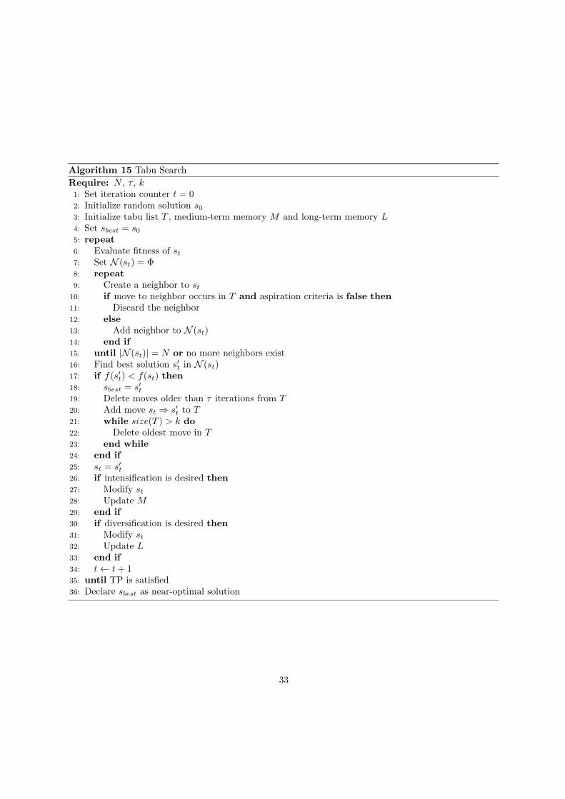
Algorithm 15 Tabu Search

Require: N , τ , k1: Set iteration counter t = 02: Initialize random solution s03: Initialize tabu list T , medium-term memory M and long-term memory L4: Set sbest = s05: repeat6: Evaluate fitness of st7: Set N (st) = Φ8: repeat9: Create a neighbor to st

10: if move to neighbor occurs in T and aspiration criteria is false then11: Discard the neighbor12: else13: Add neighbor to N (st)14: end if15: until |N (st)| = N or no more neighbors exist16: Find best solution s′t in N (st)17: if f(s′t) < f(st) then18: sbest = s′t19: Delete moves older than τ iterations from T20: Add move st ⇒ s′t to T21: while size(T ) > k do22: Delete oldest move in T23: end while24: end if25: st = s′t26: if intensification is desired then27: Modify st28: Update M29: end if30: if diversification is desired then31: Modify st32: Update L33: end if34: t← t+ 135: until TP is satisfied36: Declare sbest as near-optimal solution

33

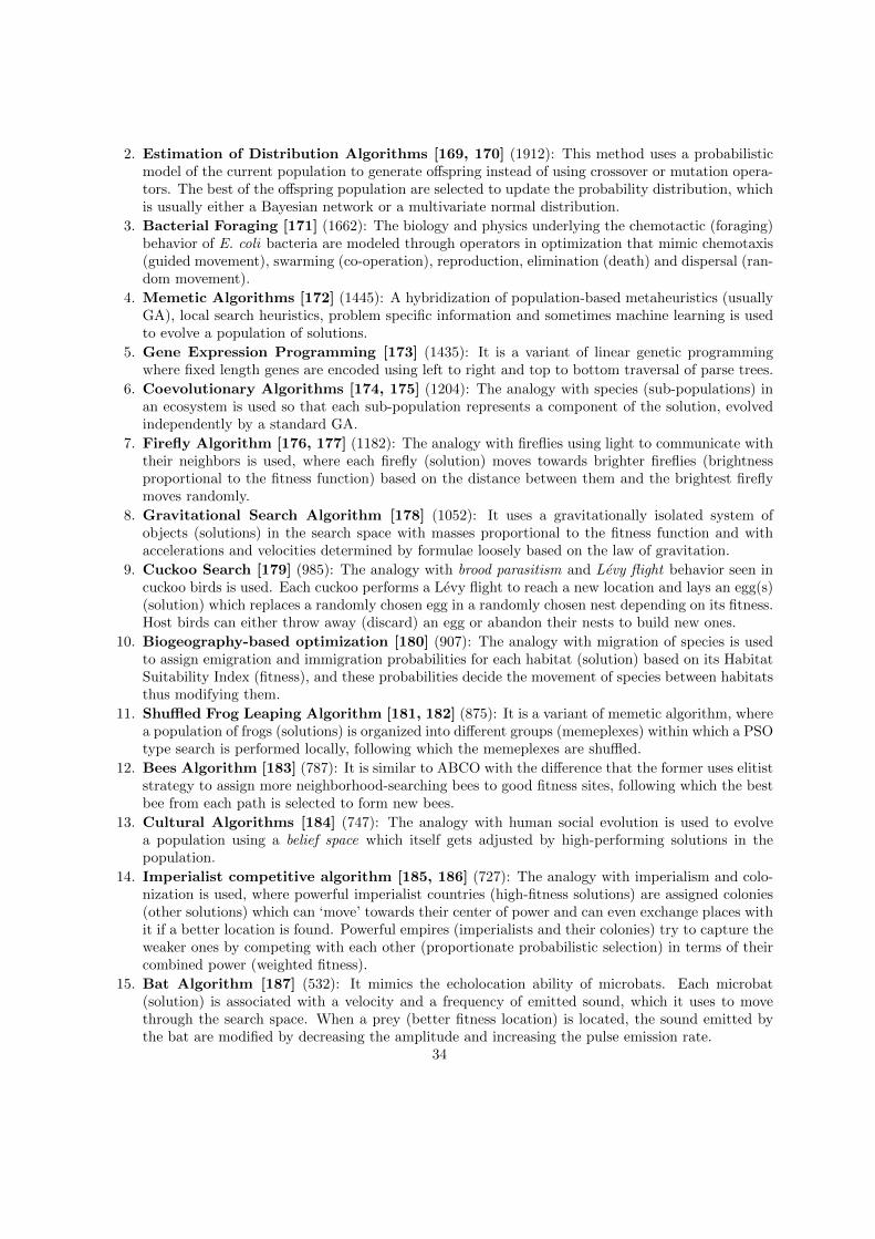
2. Estimation of Distribution Algorithms [169, 170] (1912): This method uses a probabilisticmodel of the current population to generate offspring instead of using crossover or mutation opera-tors. The best of the offspring population are selected to update the probability distribution, whichis usually either a Bayesian network or a multivariate normal distribution.

3. Bacterial Foraging [171] (1662): The biology and physics underlying the chemotactic (foraging)behavior of E. coli bacteria are modeled through operators in optimization that mimic chemotaxis(guided movement), swarming (co-operation), reproduction, elimination (death) and dispersal (ran-dom movement).

4. Memetic Algorithms [172] (1445): A hybridization of population-based metaheuristics (usuallyGA), local search heuristics, problem specific information and sometimes machine learning is usedto evolve a population of solutions.

5. Gene Expression Programming [173] (1435): It is a variant of linear genetic programmingwhere fixed length genes are encoded using left to right and top to bottom traversal of parse trees.

6. Coevolutionary Algorithms [174, 175] (1204): The analogy with species (sub-populations) inan ecosystem is used so that each sub-population represents a component of the solution, evolvedindependently by a standard GA.

7. Firefly Algorithm [176, 177] (1182): The analogy with fireflies using light to communicate withtheir neighbors is used, where each firefly (solution) moves towards brighter fireflies (brightnessproportional to the fitness function) based on the distance between them and the brightest fireflymoves randomly.

8. Gravitational Search Algorithm [178] (1052): It uses a gravitationally isolated system ofobjects (solutions) in the search space with masses proportional to the fitness function and withaccelerations and velocities determined by formulae loosely based on the law of gravitation.

9. Cuckoo Search [179] (985): The analogy with brood parasitism and Levy flight behavior seen incuckoo birds is used. Each cuckoo performs a Levy flight to reach a new location and lays an egg(s)(solution) which replaces a randomly chosen egg in a randomly chosen nest depending on its fitness.Host birds can either throw away (discard) an egg or abandon their nests to build new ones.

10. Biogeography-based optimization [180] (907): The analogy with migration of species is usedto assign emigration and immigration probabilities for each habitat (solution) based on its HabitatSuitability Index (fitness), and these probabilities decide the movement of species between habitatsthus modifying them.

11. Shuffled Frog Leaping Algorithm [181, 182] (875): It is a variant of memetic algorithm, wherea population of frogs (solutions) is organized into different groups (memeplexes) within which a PSOtype search is performed locally, following which the memeplexes are shuffled.

12. Bees Algorithm [183] (787): It is similar to ABCO with the difference that the former uses elitiststrategy to assign more neighborhood-searching bees to good fitness sites, following which the bestbee from each path is selected to form new bees.

13. Cultural Algorithms [184] (747): The analogy with human social evolution is used to evolvea population using a belief space which itself gets adjusted by high-performing solutions in thepopulation.

14. Imperialist competitive algorithm [185, 186] (727): The analogy with imperialism and colo-nization is used, where powerful imperialist countries (high-fitness solutions) are assigned colonies(other solutions) which can ‘move’ towards their center of power and can even exchange places withit if a better location is found. Powerful empires (imperialists and their colonies) try to capture theweaker ones by competing with each other (proportionate probabilistic selection) in terms of theircombined power (weighted fitness).

15. Bat Algorithm [187] (532): It mimics the echolocation ability of microbats. Each microbat(solution) is associated with a velocity and a frequency of emitted sound, which it uses to movethrough the search space. When a prey (better fitness location) is located, the sound emitted bythe bat are modified by decreasing the amplitude and increasing the pulse emission rate.

34

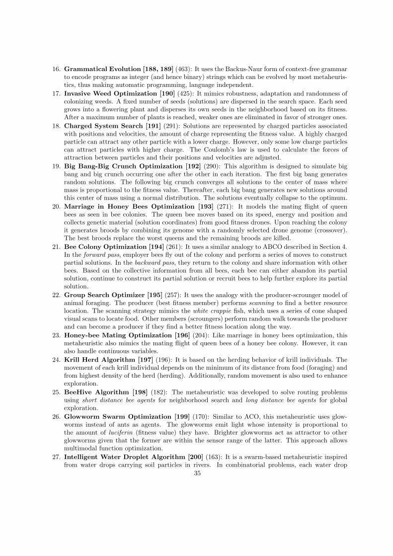
16. Grammatical Evolution [188, 189] (463): It uses the Backus-Naur form of context-free grammarto encode programs as integer (and hence binary) strings which can be evolved by most metaheuris-tics, thus making automatic programming, language independent.

17. Invasive Weed Optimization [190] (425): It mimics robustness, adaptation and randomness ofcolonizing weeds. A fixed number of seeds (solutions) are dispersed in the search space. Each seedgrows into a flowering plant and disperses its own seeds in the neighborhood based on its fitness.After a maximum number of plants is reached, weaker ones are eliminated in favor of stronger ones.

18. Charged System Search [191] (291): Solutions are represented by charged particles associatedwith positions and velocities, the amount of charge representing the fitness value. A highly chargedparticle can attract any other particle with a lower charge. However, only some low charge particlescan attract particles with higher charge. The Coulomb’s law is used to calculate the forces ofattraction between particles and their positions and velocities are adjusted.

19. Big Bang-Big Crunch Optimization [192] (290): This algorithm is designed to simulate bigbang and big crunch occurring one after the other in each iteration. The first big bang generatesrandom solutions. The following big crunch converges all solutions to the center of mass wheremass is proportional to the fitness value. Thereafter, each big bang generates new solutions aroundthis center of mass using a normal distribution. The solutions eventually collapse to the optimum.

20. Marriage in Honey Bees Optimization [193] (271): It models the mating flight of queenbees as seen in bee colonies. The queen bee moves based on its speed, energy and position andcollects genetic material (solution coordinates) from good fitness drones. Upon reaching the colonyit generates broods by combining its genome with a randomly selected drone genome (crossover).The best broods replace the worst queens and the remaining broods are killed.

21. Bee Colony Optimization [194] (261): It uses a similar analogy to ABCO described in Section 4.In the forward pass, employer bees fly out of the colony and perform a series of moves to constructpartial solutions. In the backward pass, they return to the colony and share information with otherbees. Based on the collective information from all bees, each bee can either abandon its partialsolution, continue to construct its partial solution or recruit bees to help further explore its partialsolution.

22. Group Search Optimizer [195] (257): It uses the analogy with the producer-scrounger model ofanimal foraging. The producer (best fitness member) performs scanning to find a better resourcelocation. The scanning strategy mimics the white crappie fish, which uses a series of cone shapedvisual scans to locate food. Other members (scroungers) perform random walk towards the producerand can become a producer if they find a better fitness location along the way.

23. Honey-bee Mating Optimization [196] (204): Like marriage in honey bees optimization, thismetaheuristic also mimics the mating flight of queen bees of a honey bee colony. However, it canalso handle continuous variables.

24. Krill Herd Algorithm [197] (196): It is based on the herding behavior of krill individuals. Themovement of each krill individual depends on the minimum of its distance from food (foraging) andfrom highest density of the herd (herding). Additionally, random movement is also used to enhanceexploration.

25. BeeHive Algorithm [198] (182): The metaheuristic was developed to solve routing problemsusing short distance bee agents for neighborhood search and long distance bee agents for globalexploration.

26. Glowworm Swarm Optimization [199] (170): Similar to ACO, this metaheuristic uses glow-worms instead of ants as agents. The glowworms emit light whose intensity is proportional tothe amount of luciferin (fitness value) they have. Brighter glowworms act as attractor to otherglowworms given that the former are within the sensor range of the latter. This approach allowsmultimodal function optimization.

27. Intelligent Water Droplet Algorithm [200] (163): It is a swarm-based metaheuristic inspiredfrom water drops carrying soil particles in rivers. In combinatorial problems, each water drop

35

gradually builds a solution as it moves and increases its velocity according to the soil content of thepath. More soil corresponds to a lower increase in velocity. Over iterations, paths with lesser soilcontent are preferred probabilistically.

28. Bee System [201] (133): It adopts the honey bee colony analogy to solve combinatorial problems.For example, in the traveling salesman problem, the nectar quantity represents the length of thepath. The bees are allowed to fly to any node with a probability that decreases with increasingdistance from their current location. The influence of this distance increases with iterations, makingsearch more random at the beginning and more restricted towards the end.

29. Stochastic Diffusion Search [202] (120): It uses agents with hypotheses communicating directlywith each other. In the test phase, each agent evaluates its hypothesis and finds it to be eithersuccessful or unsuccessful. In the diffusion phase, agents with unsuccessful hypotheses either selectother agents to follow or generate new hypotheses.

30. Cat Swarm optimization [203] (108): As the name suggests, the algorithm attempts to modelthe behavior of cats which represent solutions having position and velocity. Each cat has two modesof movement in the search space: the seeking mode and the tracking. The former plays the role ofthe local search component of the metaheuristic while the later tends to global search.

31. Central Force Optimization [204] (96): It also uses the analogy with particle motion undergravitational force like gravitational search algorithm, although with different formulations. Centralforce optimization is inherently deterministic unlike most other metaheuristics.

32. Queen-bee Evolution [205] (95): It is basically an integration of queen bee’s mating flight be-havior with genetic algorithms. Instead of randomly selecting parents for crossover, each individualmates with the queen bee (best fitness individual of previous generation). The mutation operationis also modified.

33. Cooperative Bees Swarm Optimization [206] (94): Unlike other bee algorithms, this methodstarts with a single bee which provides the best location based on neighborhood search. Otherbees are then recruited to a specified region around the best known location. After performingneighborhood searches, all bees communicate their individual best locations to the swarm. A tabulist of visited locations is also maintained to avoid cycles.

34. Artificial Fish Swarm Optimization [207] (91): It tries to mimic the social behavior of fishessuch as preying for food, swarming and following their neighbors. Each fish performs a local searchby visually examining its surroundings and moving towards a better food source (objective value).It may also either swarm another fish’s food source or simply follow one of its neighbors.

35. Eagle Strategy [208] (91): It uses the foraging behavior of eagles as a metaheuristic. Eaglesrepresenting candidate solutions initially perform a slow search where they search a larger areausing differential evolution. Once promising regions (prey) are identified the chasing phase beginswhich uses a fast and local search algorithms such as hill-climbing methods.

36. Differential Search Algorithm [209] (89): This algorithm simulates the Brownian-like random-walk movement used by various organisms to migrate as a superorganism. Each superorganismrepresents a candidate solution and each of its members corresponds to one variable dimension. Assuperorganisms move in the search space they exchange information about their best location withother superorganisms.

37. Backtracking Search Optimization [210] (74): It is a simplified form of evolutionary algorithmwhich uses the following operations: initialization, selection-1, mutation, crossover and selection-2.Selection-1 uses the best of the historical population members to generate a population. Mutationmutates the current population using the output of selection-1. Crossover recombines the bestindividuals of the mutant population and finally selection-2 uses greedy selection to update thecurrent population with better offspring if found.

38. Flower Pollination Algorithm [211] (61): Each solution is represented by a pollen gamete froma flowering plant. Flower pollen are carried by pollinators such as insects which move according toLevy flights. All gametes either combine with the fittest pollen (global pollination) with a givenprobability or randomly combine with other pollen gametes (local pollination).

36

39. Analytic Programming [212] (58): This metaheuristic is capable of generating programs and canbe used for symbolic regression. Unlike genetic programming, it can be used with any evolutionaryalgorithm since it acts as a superstructure requiring no changes to the variation operators.

40. Fish School Search [213, 214] (54): It uses the analogy with feeding, swimming and breedingbehavior found in fish schools. Feeding of a fish is analogous to a candidate solutions’ fitness value.Thus, the fish can gain or lose weight depending on the regions it swims in. Swimming and breedingrefer to the actual search process where solutions swarm potential regions.

41. Black Hole Optimization [215] (54): It mimics the gravitation interaction of a black hole withnearby stars. The best solution in the current population becomes the black hole and attracts othersolutions. Other stars may become a black hole if they reach a point with better fitness than thecurrent black hole. When a solution passes the event horizon of the current black hole, it vanishesand a new star (solution) is randomly initialized.

42. Monkey Search [216] (51): The solutions are analogous to monkeys and undergo climb, watch-jump and somersault steps. The climb step acts like a local optimizer for each monkey. Thewatch-jump step represents exchange of fitness landscape information and the somersault stepenable exploration of new regions in the search space.

43. Bacterial Swarming Algorithm [217] (50): This metaheuristic uses the tumble-and-run be-havior of a bacterium’s chemotactic process. The tumble operation acts like the global searchcomponent, where each bacterium (solution) moves independently to find good regions. Thereafter,the run operation causes local search.

44. Water Cycle Algorithm [218] (49): It is loosely based on the hydrologic cycle which consists ofprecipitation (random initialization of solutions), percolation into the sea (attraction towards thebest solution), evaporation and again precipitation (reinitialization of some solutions).

45. Gaussian Adaptation [219] (49): Similar in principle to CMA-ES, this method samples singlecandidate solutions from a multivariate normal distribution and iteratively updates its mean andcovariance so as to maximize the entropy of the search distribution. Strategy parameters are eitherfixed or adapted as in CMA-ES.

46. River Formation Dynamics [220] (45): It is used to solve the traveling salesman problem usingthe analogy with a flowing river eroding soil from high altitudes and depositing it at lower altitudes.Initially all nodes are at the same altitude. But as the water drops move from origin to destinationthey erode various edges until all drops follow the same path.

47. Brain Storm Optimization [221] (40): The solutions are considered as individuals coming upwith different ideas during a brain storming session. The best ideas are selected and new ideas arecreated based on their combinations. Individuals with rejected ideas try to come up with new ideas(reinitialization).

48. Roach Infestation Optimization [222] (39): It mimics the collective behavior of cockroaches infinding dark regions in an enclosed space. The level of darkness is proportional to the fitness value.Initially each roach (solution) acts individually to find a dark region. However, when it comes inclose proximity to another roach they exchange information about their respective regions. Theinformation of the darkest known location will thus spread through the roach population.

49. League Championship Algorithm [223] (35): It is based on the metaphor of sporting com-petitions in sport leagues. Each candidate solution is a team and its position in the search spacedefines the team’s strategy. Each week (iteration) the teams participate in pairwise competitionsand based on their ranking modify their strategies.

50. Electro-magnetism Optimization [224] (31): It is similar in principle to charged system search.Charge particles represent solutions which move under the influence of electrostatic forces. Thenature of the force on a particle (attractive or repulsive) due to another particle depends on thecharge (fitness) of the other particle. Therefore, the motion does not strictly conform to physicalelectrostatic laws.

37

51. Galaxy-based Search [225] (25): It uses the metaphor of the spiraling arms of a galaxy sweepingthe solution space to find better regions. This step is referred to as the spiral chaotic move.Thereafter, local search is performed within these regions to fine-tune the obtained solutions.

52. Dolphin Echolocation [226] (24): It mimics the echolocation ability of dolphins to find prey.Solutions (echoes) are initially randomly distributed in the search space. The fitness (echo quality)at each location is evaluated and more or less echoes are allocated in the neighborhood of eachlocation based on the fitness values.

53. Wolf Search Algorithm [227] (20): The analogy with wolfs hunting for prey in packs is used inthis algorithms. Each wolf (solution) has a fixed visual area and can sense companions within it.The quality of a wolf’s position is represented by the fitness value of the solutions. A wolf whichhas a better placed companion in its sight moves towards it. At times, a wolf may sense an enemyand sprint to a random location (reinitialization).

54. Artificial Cooperative Search [228] (20): It uses two populations referred to as superorganisms.Each superorganism is a collection of sub-superorganisms (solutions) and each sub-superorganismis a collection of variable dimensions (i.e. a solution). The sub-superorganisms have a predator-prey relationship based on the relative fitness values. Whether a superorganism is the prey or thepredator is determined randomly in each generation.

55. Rubber Band Technique based GA [229] (20): This method is specifically targeted to solvemultiple sequence alignment problems encountered in bioinformatics. It is inspired by the behaviorof an elastic rubber band on a plate with several poles. The poles can either be primary (throughwhich the band ought to pass) or secondary. GA is used to arrive at the rubber band configurationwhich best addresses the sequence alignment problem.

56. Bacterial-GA Foraging [230] (19): It combines bacterial foraging algorithm with GA. In additionto tumble and swim, the bacteria (solutions) also undergo crossover and mutation as in a GA. Whenindividuals are eliminated, new individuals are formed by mutating the eliminated ones instead ofrandom reinitialization.

57. Spiral Dynamics Inspired Optimization [231] (19): The population consists candidate solu-tions, each forming the center of a spiral. The shape and size of the spirals is determined by twoparameters, the rotation angle and the convergence rate to the center. These parameters controlthe diversification and intensification of the spiral around the solution. Spirals corresponding tohigh fitness centers tend towards intensification.

58. Great Salmon Run Algorithm [232] (16): The algorithm takes its inspiration from the salmonrun phenomenon where millions of salmons migrate upstream for spawning even risking becomingprey. Each solution represents a salmon sub-group that selects a migration pathway. Differentpathways pose different threats to the sub-group, like either being hunted by humans or by bears.At the end, salmons from safer pathways spawn to produce offspring which are more likely to takesafer pathways.

59. Paddy Field Algorithm [233] (15): It uses the analogy with paddy fields where the seeds laidin the most fertile (high fitness) region of the field (search space) grow to produce more seeds. Theseeds represent solutions and therefore eventually the optimum gets crowded.

60. Japanese Tree Frogs Algorithm [234] (13): The algorithm simulates the mating behavior ofmale tree frogs which intentionally desynchronize their mating calls to allow female frogs to correctlylocalize them. The analogy is used to solve the graph coloring problem, whose optimization versionaims to minimize the number of colors to be used.

61. Consultant-guided Search [235] (13): Each solution in the population is a virtual person whocan act both as a client and a consultant. The reputation of a person as a consultant depends onthe number of successes achieved by its clients following the person’s advice. Reputation can eitherincrease or decrease, but when it falls below a certain value the person takes a sabbatical leave(reinitialization) and stops giving advice.

62. Hierarchical Swarm Model [236] (13): It generalizes the standard flat framework of swarmintelligence methods. Instead of all particles interacting with each other, this method introduces a

38

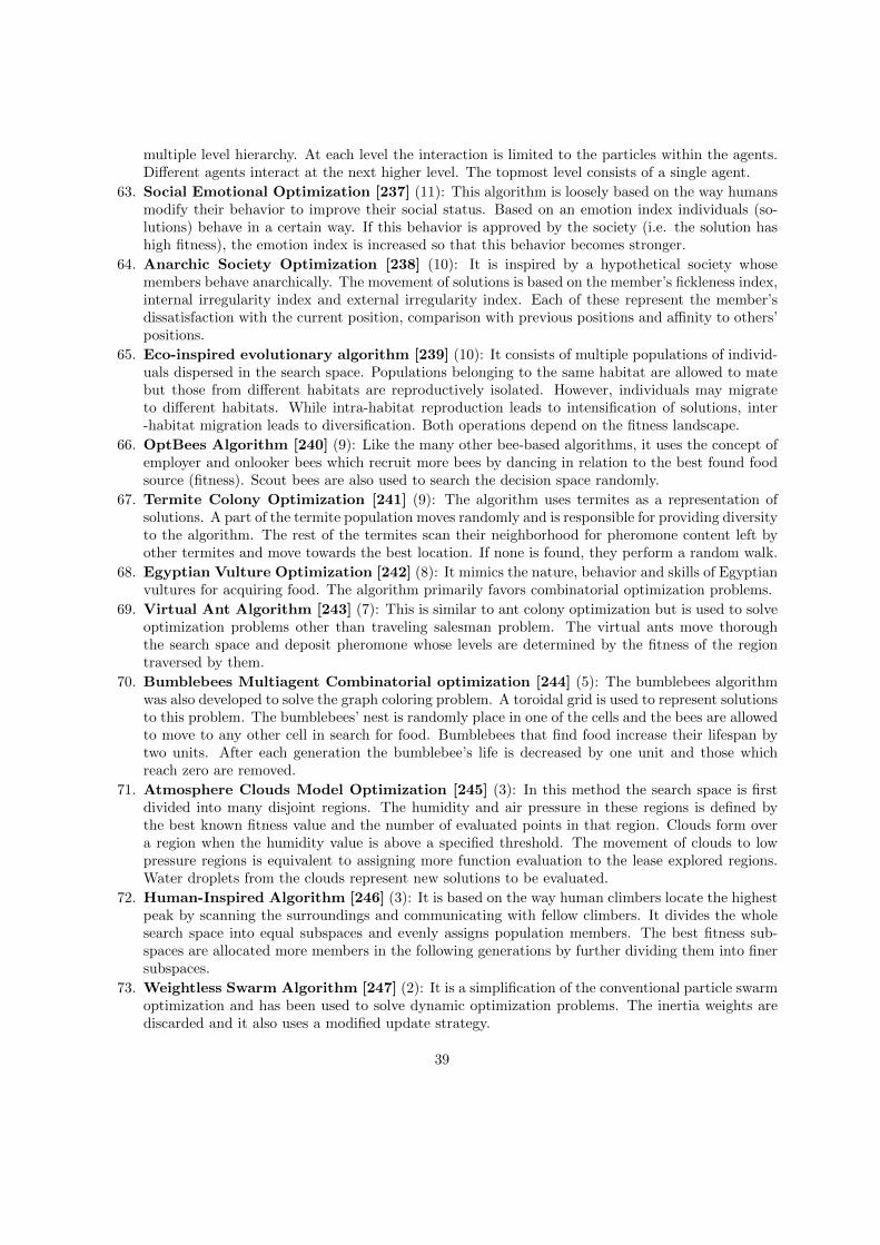
multiple level hierarchy. At each level the interaction is limited to the particles within the agents.Different agents interact at the next higher level. The topmost level consists of a single agent.

63. Social Emotional Optimization [237] (11): This algorithm is loosely based on the way humansmodify their behavior to improve their social status. Based on an emotion index individuals (so-lutions) behave in a certain way. If this behavior is approved by the society (i.e. the solution hashigh fitness), the emotion index is increased so that this behavior becomes stronger.

64. Anarchic Society Optimization [238] (10): It is inspired by a hypothetical society whosemembers behave anarchically. The movement of solutions is based on the member’s fickleness index,internal irregularity index and external irregularity index. Each of these represent the member’sdissatisfaction with the current position, comparison with previous positions and affinity to others’positions.

65. Eco-inspired evolutionary algorithm [239] (10): It consists of multiple populations of individ-uals dispersed in the search space. Populations belonging to the same habitat are allowed to matebut those from different habitats are reproductively isolated. However, individuals may migrateto different habitats. While intra-habitat reproduction leads to intensification of solutions, inter-habitat migration leads to diversification. Both operations depend on the fitness landscape.

66. OptBees Algorithm [240] (9): Like the many other bee-based algorithms, it uses the concept ofemployer and onlooker bees which recruit more bees by dancing in relation to the best found foodsource (fitness). Scout bees are also used to search the decision space randomly.

67. Termite Colony Optimization [241] (9): The algorithm uses termites as a representation ofsolutions. A part of the termite population moves randomly and is responsible for providing diversityto the algorithm. The rest of the termites scan their neighborhood for pheromone content left byother termites and move towards the best location. If none is found, they perform a random walk.

68. Egyptian Vulture Optimization [242] (8): It mimics the nature, behavior and skills of Egyptianvultures for acquiring food. The algorithm primarily favors combinatorial optimization problems.

69. Virtual Ant Algorithm [243] (7): This is similar to ant colony optimization but is used to solveoptimization problems other than traveling salesman problem. The virtual ants move thoroughthe search space and deposit pheromone whose levels are determined by the fitness of the regiontraversed by them.

70. Bumblebees Multiagent Combinatorial optimization [244] (5): The bumblebees algorithmwas also developed to solve the graph coloring problem. A toroidal grid is used to represent solutionsto this problem. The bumblebees’ nest is randomly place in one of the cells and the bees are allowedto move to any other cell in search for food. Bumblebees that find food increase their lifespan bytwo units. After each generation the bumblebee’s life is decreased by one unit and those whichreach zero are removed.

71. Atmosphere Clouds Model Optimization [245] (3): In this method the search space is firstdivided into many disjoint regions. The humidity and air pressure in these regions is defined bythe best known fitness value and the number of evaluated points in that region. Clouds form overa region when the humidity value is above a specified threshold. The movement of clouds to lowpressure regions is equivalent to assigning more function evaluation to the lease explored regions.Water droplets from the clouds represent new solutions to be evaluated.

72. Human-Inspired Algorithm [246] (3): It is based on the way human climbers locate the highestpeak by scanning the surroundings and communicating with fellow climbers. It divides the wholesearch space into equal subspaces and evenly assigns population members. The best fitness sub-spaces are allocated more members in the following generations by further dividing them into finersubspaces.

73. Weightless Swarm Algorithm [247] (2): It is a simplification of the conventional particle swarmoptimization and has been used to solve dynamic optimization problems. The inertia weights arediscarded and it also uses a modified update strategy.

39

74. Good Lattice Swarm Algorithm [248] (1): It replaces the random initialization of particlesand their velocities in particle swarm optimization with a good lattice uniform distribution, whichaccording to number theory, has the least discrepancy.

75. Photosynthetic Algorithm [249] (1): This algorithm uses the analogy with carbon moleculestransforming from one substance to another during Calvin-Benson cycle and mimics the reactiontaking place in the chloroplast during photorespiration for recombining different solutions.

76. Eurygaster Algorithm [250] (0): It mimics the behavior of eurygasters attacking grain farmsin different groups always settling for the closest unattacked regions of the farm. The method hasbeen applied to graph partitioning problem.

Many such methods are yet to be discovered and practiced, but an interesting future research would be toidentify essential differences among these algorithms and specific features that make each of them uniqueand efficient in solving a specific class of optimization problems. Recent approaches [251, 252, 253] inthis direction have provided useful insights about similarities of a few metaheuristic methodologies.

Despite their success and popularity, metaheuristic techniques have received some criticism over theyears. The main criticism concerns their non-mathematical nature and lack of a proof of convergence.Due to the stochasticity involved, it is difficult to derive an exact theory of how these algorithms work.Few theoretical analyses do exist for some of the methods. However, they often relate to a simplifiedand basic version of the algorithm. While there is no immediate remedy for this, the best approach forpractitioners is to provide empirical results on a wide variety of benchmark test problems available inliterature. Reproducibility of results is an essential part of dissemination in this regard. In order toachieve this under stochasticity, uniformly seeded pseudo random number generators are used and thealgorithm is run several times. A common practice is to use statistical analysis to draw conclusions fromsuch empirical studies.

Recent criticism has been with respect to the ever growing number of “novel” metaheuristics as isevident from the list above. Sorensen [254] argues that many of these recently proposed metaheuristicsare similar in almost all respects except the metaphor that is used to describe them. For example, in[255] and [256] the author shows that one of the recent metaheuristics, harmony search, is a special caseof evolutionary strategy. Sorensen also points out that the terminology used to convey and justify themetaphor sometimes completely obfuscates the similarities with existing methods. Indeed, as describedin Section 2, all metaheuristics have two major characteristics, exploration and exploitation. There maybe several different ways of accomplishing these tasks in an algorithm, but calling each such method“new”, “novel” and “innovative” would be pushing the metaphor too far. The major disadvantage of theundeserved attention that many of these recent techniques get is the distraction it causes away from keydevelopments in the field of metaheuristics.

16. Conclusions

The present paper began with a discussion on the main concepts concerning metaheuristics such astheir classification and characteristics. We laid down a generic framework into which most metaheuristictechniques can fit. The key components essential to the working of any metaheuristic were identifiedunder five plans, namely selection, generation, replacement, update and termination. Some importantparameters were also introduced. Thereafter, we reviewed a number of popular metaheuristic methodsfor solving optimization problems. Pseudocodes have been provided for 14 of the most commonly usedmethods for ease of understanding and implementation. Key variants of some of the algorithms werealso discussed. Except simulated annealing and tabu search, all other methods are population-based.Moreover, we mainly concentrated on evolutionary and swarm-based methods, which are older, well-known and frequently used. For completeness, we have included an extensive list of other metaheuristicsand ordered them by their Google Scholar citations. Though this metric may not be a true count ofcitations, it serves as a measure of popularity of these methods. Finally, we briefly discussed the criticismthat the field of metaheuristics currently faces.

40

A recent trend in the field of metaheuristics is hybridization. This not only refers to the combinationof different available metaheuristics but also to their integration with classical search methods. Classicalalgorithms are efficient local optimizers and therefore can aid the intensification process. Not surprisingly,such hybrid methods have been shown to outperform standalone methods. Hybrid-metaheuristics alsorefer to the use of data-mining and machine learning techniques to enhance search. With the increasedaccessibility to computing power, resource and memory-intensive tasks like data-mining can now beperformed alongside metaheuristic optimization to learn patterns, predict outcomes and assist the searchbehavior.

Parallel metaheuristics can refer to different levels of parallelization, algorithmic level, iteration leveland solution level. Algorithmic level involves multiple metaheuristics running simultaneously, commu-nicating and collaborating with each other to solve a complex search problem. Iteration level involvesparallelizing the operations within an iteration. This is especially useful in population-based metaheuris-tics. Solution level parallelization pertains to individual solutions. For example, if the evaluation of theobjective function involves a finite element analysis, then this analysis itself can be parallelized. All theseare very active and relevant areas of research within metaheuristics.

Another common research problem that needs to be addressed is that of setting the best parameters forthe algorithm at hand. It is well-known that for most metaheuristics the performance can be drasticallyaffected through their parameters. Parameter tuning refers to the selection of the best configuration ofthe algorithm for solving a particular problem. Both offline and online parameter tuning methods havebeen proposed in literature. However, like with optimization algorithms, there is no one best approach.

Metamodeling is an entire research area in itself. As metamodels are increasingly being used withinoptimization, more empirical studies need to be performed on the compatibility of different metamodelswith different metaheuristics. Again, it is improbable that one unique combination will emerge as thewinner. However, these studies can give a lot of insight about which methods work best on specificuse-cases.

Metaheuristics have been and will continue to be used to solve complex optimization problems. Insteadof developing more and more new algorithms, the focus should now shift towards improving currentalgorithms by unifying different ideas into a common and generic framework as the one described in thispaper. There is also a growing need for classifying different metaheuristic methods according to theirfunctional or algorithmic similarities. The algorithmic connection between two such methods providesa way to introduce one algorithm’s key feature into another algorithm, a matter that will help unifydifferent metaheuristic methods under one umbrella of a meta-algorithm for solving complex real-worldoptimization problems.

Acknowledgments

The first author acknowledges the financial support received from The Knowledge Foundation (KK-stiftelsen, Stockholm, Sweden) for the ProSpekt project KDISCO.

References

[1] E.-G. Talbi, Metaheuristics: From design to implementation. Hoboken, New Jersey, USA: John Wiley & Sons, 2009.[2] G. Zapfel, R. Braune, and M. Bogl, Metaheuristic search concepts: A tutorial with applications to production and

logistics. Heidelberg: Springer Science & Business Media, 2010.[3] M. Gendreau and J.-Y. Potvin, Handbook of metaheuristics. New York, USA: Springer, 2010.[4] S. Luke, Essentials of Metaheuristics. Lulu, 2013. Available for free at

http://cs.gmu.edu/∼sean/book/metaheuristics/.[5] C. C. Ribeiro and P. Hansen, Essays and surveys in metaheuristics. New York, USA: Springer Science & Business

Media, 2012.[6] F. Glover and G. A. Kochenberger, Handbook of metaheuristics. Dordrecht: Kluwer Academic Publishers, 2003.[7] I. H. Osman and J. P. Kelly, Meta-heuristics: Theory and applications. Norwell, Massachusetts, USA: Kluwer

Academic Publishers, 2012.

41

[8] S. Voß, S. Martello, I. H. Osman, and C. Roucairol, Meta-heuristics: Advances and trends in local search paradigmsfor optimization. New York, USA: Springer Science & Business Media, 2012.

[9] T. F. Gonzalez, Handbook of approximation algorithms and metaheuristics. Boca Raton, FL, USA: CRC Press, 2007.[10] J. Dreo, A. Petrowski, P. Siarry, and E. Taillard, Metaheuristics for hard optimization: Methods and case studies.

Berlin Heidelberg: Springer Science & Business Media, 2006.[11] P. Siarry and Z. Michalewicz, Advances in metaheuristics for hard optimization. Berlin Heidelberg: Springer Science

& Business Media, 2007.[12] K. F. Doerner, M. Gendreau, P. Greistorfer, W. Gutjahr, R. F. Hartl, and M. Reimann, Metaheuristics: Progress in

complex systems optimization. New York, USA: Springer Science & Business Media, 2007.[13] X.-S. Yang, Nature-inspired optimization algorithms. London, UK: Elsevier, 2014.[14] D. F. Jones, S. K. Mirrazavi, and M. Tamiz, “Multi-objective meta-heuristics: An overview of the current state-of-

the-art,” European Journal of Operational Research, vol. 137, no. 1, pp. 1–9, 2002.[15] I. H. Osman and G. Laporte, “Metaheuristics: A bibliography,” Annals of Operations Research, vol. 63, no. 5,

pp. 511–623, 1996.[16] E.-G. Talbi, “A taxonomy of hybrid metaheuristics,” Journal of Heuristics, vol. 8, no. 5, pp. 541–564, 2002.[17] L. Jourdan, M. Basseur, and E.-G. Talbi, “Hybridizing exact methods and metaheuristics: A taxonomy,” European

Journal of Operational Research, vol. 199, no. 3, pp. 620–629, 2009.[18] G. R. Raidl, “A unified view on hybrid metaheuristics,” in Hybrid Metaheuristics (F. Almeida, M. J. B. Aguilera,

C. Blum, J. M. M. Vega, M. P. Perez, A. Roli, and M. Sampels, eds.), pp. 1–12, Springer, 2006.[19] I. Boussaıd, J. Lepagnot, and P. Siarry, “A survey on optimization metaheuristics,” Information Sciences, vol. 237,

pp. 82–117, 2013.[20] S. Olafsson, “Metaheuristics,” in Handbook in operations research and management science (S. Henderson and B. Nel-

son, eds.), vol. 13, pp. 633–654, Elsevier, 2006.[21] B. Melian, J. A. M. Perez, and J. M. M. Vega, “Metaheuristics: A global view,” Inteligencia Artificial, vol. 7, no. 19,

pp. 7–28, 2003.[22] C. Blum and A. Roli, “Hybrid metaheuristics: An introduction,” in Hybrid Metaheuristics (C. Blum, M. J. B.

Aguilera, A. Roli, and M. Sampels, eds.), pp. 1–30, Springer, 2008.[23] C. Rego and F. Glover, “Local search and metaheuristics,” in The traveling salesman problem and its variations

(G. Gutin and A. P. Punnen, eds.), pp. 309–368, Springer, 2007.[24] L. M. Rios and N. V. Sahinidis, “Derivative-free optimization: A review of algorithms and comparison of software

implementations,” Journal of Global Optimization, vol. 56, no. 3, pp. 1247–1293, 2013.[25] C. Blum and A. Roli, “Metaheuristics in combinatorial optimization: Overview and conceptual comparison,” ACM

Computing Surveys, vol. 35, no. 3, pp. 268–308, 2003.[26] L. Bianchi, M. Dorigo, L. M. Gambardella, and W. J. Gutjahr, “A survey on metaheuristics for stochastic combina-

torial optimization,” Natural Computing, vol. 8, no. 2, pp. 239–287, 2009.[27] M. Gendreau and J.-Y. Potvin, “Metaheuristics in combinatorial optimization,” Annals of Operations Research,

vol. 140, no. 1, pp. 189–213, 2005.[28] C. Blum, J. Puchinger, G. R. Raidl, and A. Roli, “Hybrid metaheuristics in combinatorial optimization: A survey,”

Applied Soft Computing, vol. 11, no. 6, pp. 4135–4151, 2011.[29] T. G. Stutzle, Local search algorithms for combinatorial problems: Analysis, improvements, and new applications.

Amsterdam: IOS Press, 1999.[30] L. Bianchi, M. Birattari, M. Chiarandini, M. Manfrin, M. Mastrolilli, L. Paquete, O. Rossi-Doria, and T. Schiavinotto,

“Hybrid metaheuristics for the vehicle routing problem with stochastic demands,” Journal of Mathematical Modellingand Algorithms, vol. 5, no. 1, pp. 91–110, 2006.

[31] O. Braysy and M. Gendreau, “Vehicle routing problem with time windows, Part II: Metaheuristics,” TransportationScience, vol. 39, no. 1, pp. 119–139, 2005.

[32] B. L. Golden, E. A. Wasil, J. P. Kelly, and I.-M. Chao, “The impact of metaheuristics on solving the vehicle routingproblem: Algorithms, problem sets, and computational results,” in Fleet management and logistics (T. G. Crainicand G. Laporte, eds.), pp. 33–56, Springer, 1998.

[33] W.-C. Chiang and R. A. Russell, “Simulated annealing metaheuristics for the vehicle routing problem with timewindows,” Annals of Operations Research, vol. 63, no. 1, pp. 3–27, 1996.

[34] J. Puchinger and G. R. Raidl, Combining metaheuristics and exact algorithms in combinatorial optimization: Asurvey and classification. Berlin Heidelberg: Springer, 2005.

[35] M. Birattari, L. Paquete, T. Stutzle, and K. Varrentrapp, “Classification of metaheuristics and design of experimentsfor the analysis of components,” tech. rep., Darmstadt University of Technology, Germany, 2001.

[36] D. J. Rosenkrantz, R. E. Stearns, and P. M. Lewis, II, “An analysis of several heuristics for the traveling salesmanproblem,” SIAM Journal on Computing, vol. 6, no. 3, pp. 563–581, 1977.

[37] W. J. Gutjahr, “Convergence analysis of metaheuristics,” in Matheuristics (V. Maniezzo, T. Stutzle, and S. Voß,eds.), pp. 159–187, Springer, 2010.

[38] X.-S. Yang, “Metaheuristic optimization: Algorithm analysis and open problems,” in Experimental Algorithms (P. M.Pardalos and S. Rebennack, eds.), pp. 21–32, Springer, 2011.

[39] T. Stutzle and S. Fernandes, “New benchmark instances for the QAP and the experimental analysis of algorithms,” inEvolutionary Computation in Combinatorial Optimization (J. Gottlieb and G. R. Raidl, eds.), pp. 199–209, Springer,2004.

42

[40] M. Birattari, T. Stutzle, L. Paquete, and K. Varrentrapp, “A racing algorithm for configuring metaheuristics,” inProceedings of the Genetic and Evolutionary Computation Conference, vol. 2, pp. 11–18, 2002.

[41] M. Birattari and M. Dorigo, The problem of tuning metaheuristics as seen from a machine learning perspective. PhDthesis, Universite Libre de Bruxelles, 2004.

[42] O. Rossi-Doria, M. Sampels, M. Birattari, M. Chiarandini, M. Dorigo, L. M. Gambardella, J. Knowles, M. Manfrin,M. Mastrolilli, B. Paechter, L. Paquete, and T. Stutzle, “A comparison of the performance of different metaheuristicson the timetabling problem,” in Practice and Theory of Automated Timetabling IV (E. Burke and P. D. Causmaecker,eds.), pp. 329–351, Springer, 2003.

[43] E. Alba, G. Luque, and E. Alba, “Measuring the performance of parallel metaheuristics,” in Parallel Metaheuristics:A New Class of Algorithms (E. Alba, ed.), vol. 47, pp. 43–62, John Wiley & Sons, 2005.

[44] T. G. Crainic and M. Toulouse, Parallel strategies for meta-heuristics. New York, USA: Springer, 2003.[45] E. Alba, Parallel metaheuristics: A new class of algorithms. Hoboken, New Jersey, USA: John Wiley & Sons, 2005.[46] V.-D. Cung, S. L. Martins, C. C. Ribeiro, and C. Roucairol, “Strategies for the parallel implementation of meta-

heuristics,” in Essays and surveys in metaheuristics (C. C. Ribeiro and P. Hansen, eds.), pp. 263–308, Springer,2002.

[47] T. G. Crainic and M. Toulouse, “Parallel meta-heuristics,” in Handbook of metaheuristics (M. Gendreau and J.-Y.Potvin, eds.), pp. 497–541, Springer, 2010.

[48] S. Cahon, N. Melab, and E.-G. Talbi, “Paradiseo: A framework for the reusable design of parallel and distributedmetaheuristics,” Journal of Heuristics, vol. 10, no. 3, pp. 357–380, 2004.

[49] E.-G. Talbi, Parallel combinatorial optimization. Hoboken, New Jersey, USA: John Wiley & Sons, 2006.[50] E. Alba, G. Luque, and S. Nesmachnow, “Parallel metaheuristics: Recent advances and new trends,” International

Transactions in Operational Research, vol. 20, no. 1, pp. 1–48, 2013.[51] E. Alba and G. Luque, “Evaluation of parallel metaheuristics,” in Parallel Problem Solving from Nature, pp. 9–14,

Springer, 2006.[52] S. D. Eksioglu, P. Pardalos, and M. Resende, “Parallel metaheuristics for combinatorial optimization,” in Models for

Parallel and Distributed Computation (R. Correa, I. Dutra, M. Fiallos, and F. Gomes, eds.), Springer, 2002.[53] D. Wolpert and W. Macready, “No free lunch theorems for optimization,” IEEE Transactions on Evolutionary

Computation, vol. 1, no. 1, pp. 67–82, 1997.[54] Z. Michalewicz, “A survey of constraint handling techniques in evolutionary computation methods,” Evolutionary

Programming, vol. 4, pp. 135–155, 1995.[55] C. A. C. Coello, “Theoretical and numerical constraint-handling techniques used with evolutionary algorithms: A

survey of the state of the art,” Computer methods in applied mechanics and engineering, vol. 191, no. 11, pp. 1245–1287, 2002.

[56] K. Deb and R. Datta, “A fast and accurate solution of constrained optimization problems using a hybrid bi-objectiveand penalty function approach,” in IEEE Congress on Evolutionary Computation, pp. 165–172, IEEE, 2010.

[57] S. Camazine, J.-L. Deneubourg, N. R. Franks, J. Sneyd, G. Theraulaz, and E. Bonabeau, Self-organization in biologicalsystems. Princeton, New Jersey, USA: Princeton University Press, 2003.

[58] P. Grasse, “Recherches sur la biologie des termites champignonnistes (Macrotermitinae),” Annales des SciencesNaturelles (Zoologie), vol. 6, pp. 97–171, 1944.

[59] J.-L. Deneubourg, S. Aron, S. Goss, and J. M. Pasteels, “The self-organizing exploratory pattern of the argentineant,” Journal of Insect Behavior, vol. 3, no. 2, pp. 159–168, 1990.

[60] M. Dorigo, V. Maniezzo, and A. Colorni, “Ant system: Optimization by a colony of cooperating agents,” IEEETransactions on Systems, Man, and Cybernetics, Part B: Cybernetics, vol. 26, no. 1, pp. 29–41, 1996.

[61] E. L. Lawler, J. K. Lenstra, A. H. G. R. Kan, and D. B. Shmoys, The traveling salesman problem: A guided tour ofcombinatorial optimization. Chichester, UK: Wiley, 1985.

[62] V. Maniezzo and A. Colorni, “The ant system applied to the quadratic assignment problem,” IEEE Transactions onKnowledge and Data Engineering, vol. 11, no. 5, pp. 769–778, 1999.

[63] A. Colorni, M. Dorigo, V. Maniezzo, and M. Trubian, “Ant system for job-shop scheduling,” Belgian Journal ofOperations Research, Statistics and Computer Science, vol. 34, no. 1, pp. 39–53, 1994.

[64] B. Bullnheimer, R. F. Hartl, and C. Strauss, “Applying the ant system to the vehicle routing problem,” in Meta-Heuristics (S. Voß, S. Martello, I. H. Osman, and C. Roucairol, eds.), pp. 285–296, Springer, 1999.

[65] M. Dorigo and L. M. Gambardella, “Ant colony system: A cooperative learning approach to the traveling salesmanproblem,” IEEE Transactions on Evolutionary Computation, vol. 1, no. 1, pp. 53–66, 1997.

[66] G. Bilchev and I. C. Parmee, “The ant colony metaphor for searching continuous design spaces,” in EvolutionaryComputing (T. C. Fogarty, ed.), pp. 25–39, Springer, 1995.

[67] K. Socha and M. Dorigo, “Ant colony optimization for continuous domains,” European Journal of Operational Re-search, vol. 185, no. 3, pp. 1155–1173, 2008.

[68] M. Mathur, S. B. Karale, S. Priye, V. Jayaraman, and B. Kulkarni, “Ant colony approach to continuous functionoptimization,” Industrial & engineering chemistry research, vol. 39, no. 10, pp. 3814–3822, 2000.

[69] G. Crina and A. Ajith, “Stigmergic optimization: Inspiration, technologies and perspectives,” in Stigmergic optimiza-tion (A. Ajith, G. Crina, and R. Vitorino, eds.), pp. 1–24, Springer, 2006.

[70] D. Karaboga, “An idea based on honey bee swarm for numerical optimization,” tech. rep., Erciyes University, Turkey,2005.

[71] D. Karaboga and B. Basturk, “A powerful and efficient algorithm for numerical function optimization: Artificial bee

43

colony (ABC) algorithm,” Journal of Global Optimization, vol. 39, no. 3, pp. 459–471, 2007.[72] R. S. Rao, S. Narasimham, and M. Ramalingaraju, “Optimization of distribution network configuration for loss reduc-

tion using artificial bee colony algorithm,” International Journal of Electrical Power and Energy Systems Engineering,vol. 1, no. 2, pp. 116–122, 2008.

[73] A. Singh, “An artificial bee colony algorithm for the leaf-constrained minimum spanning tree problem,” Applied SoftComputing, vol. 9, no. 2, pp. 625–631, 2009.

[74] N. Karaboga, “A new design method based on artificial bee colony algorithm for digital iir filters,” Journal of theFranklin Institute, vol. 346, no. 4, pp. 328–348, 2009.

[75] Q.-K. Pan, M. F. Tasgetiren, P. N. Suganthan, and T. J. Chua, “A discrete artificial bee colony algorithm for thelot-streaming flow shop scheduling problem,” Information Sciences, vol. 181, no. 12, pp. 2455–2468, 2011.

[76] D. Teodorovic and M. Dell’Orco, “Bee colony optimization - A cooperative learning approach to complex transporta-tion problems,” in Proceedings of the 16th Mini-EURO Conference on Advanced OR and AI Methods in Transporta-tion, pp. 51–60, 2005.

[77] S. Omkar, J. Senthilnath, R. Khandelwal, G. N. Naik, and S. Gopalakrishnan, “Artificial bee colony (ABC) formulti-objective design optimization of composite structures,” Applied Soft Computing, vol. 11, no. 1, pp. 489–499,2011.

[78] S. F. M. Burnet, The clonal selection theory of acquired immunity. Cambridge, United Kingdom: Cambridge Uni-versity Press, 1959.

[79] L. N. De Castro and F. J. Von Zuben, “The clonal selection algorithm with engineering applications,” in Proceedingsof the Genetic and Evolutionary Computation Conference, vol. 2000, pp. 36–39, 2000.

[80] L. N. De Castro and F. J. Von Zuben, “Learning and optimization using the clonal selection principle,” IEEETransactions on Evolutionary Computation, vol. 6, no. 3, pp. 239–251, 2002.

[81] J. Timmis, C. Edmonds, and J. Kelsey, “Assessing the performance of two immune inspired algorithms and a hybridgenetic algorithm for function optimisation,” in IEEE Congress on Evolutionary Computation, vol. 1, pp. 1044–1051,IEEE, 2004.

[82] A. Gasper and P. Collard, “From GAs to artificial immune systems: Improving adaptation in time dependent opti-mization,” in IEEE Congress on Evolutionary Computation, vol. 3, IEEE, 1999.

[83] L. N. De Castro and F. J. Von Zuben, “Learning and optimization using the clonal selection principle,” IEEETransactions on Evolutionary Computation, vol. 6, no. 3, pp. 239–251, 2002.

[84] L. N. De Castro and F. J. Von Zuben, “The clonal selection algorithm with engineering applications,” in Proceedingsof the Genetic and Evolutionary Computation Conference, vol. 2000, pp. 36–39, 2000.

[85] P. Hajela and J. Lee, “Constrained genetic search via schema adaptation: An immune network solution,” StructuralOptimization, vol. 12, no. 1, pp. 11–15, 1996.

[86] X. Wang, X. Z. Gao, and S. J. Ovaska, “An immune-based ant colony algorithm for static and dynamic optimization,”in International Conference on Systems, Man and Cybernetics, pp. 1249–1255, IEEE, 2007.

[87] D. Dasgupta, An overview of artificial immune systems and their applications. Berlin Heidelberg: Springer, 1999.[88] R. Storn and K. Price, “Differential evolution - A simple and efficient heuristic for global optimization over continuous

spaces,” Journal of Global Optimization, vol. 11, no. 4, pp. 341–359, 1997.[89] J. A. Nelder and R. Mead, “A simplex method for function minimization,” The Computer Journal, vol. 7, no. 4,

pp. 308–313, 1965.[90] S. Das and P. N. Suganthan, “Differential evolution: A survey of the state-of-the-art,” IEEE Transactions on Evo-

lutionary Computation, vol. 15, no. 1, pp. 4–31, 2011.[91] R. Storn and K. Price, “Minimizing the real functions of the icec’96 contest by differential evolution,” in IEEE

International Conference on Evolutionary Computation, pp. 842–844, IEEE, 1996.[92] K. V. Price, R. M. Storn, and J. A. Lampinen, Differential evolution - A practical approach to global optimization.

Berlin Heidelberg: Springer-Verlag, 2005.[93] V. Feoktistov and S. Janaqi, “Generalization of the strategies in differential evolution,” in Proceedings of the 18th

International Parallel and Distributed Processing Symposium, pp. 2341–2346, IEEE, 2004.[94] H.-Y. Fan and J. Lampinen, “A trigonometric mutation operation to differential evolution,” Journal of Global Opti-

mization, vol. 27, no. 1, pp. 105–129, 2003.[95] K. V. Price, “An introduction to differential evolution,” in New ideas in optimization (D. Corne, M. Dorigo, F. Glover,

D. Dasgupta, P. Moscato, R. Poli, and K. V. Price, eds.), pp. 79–108, McGraw-Hill, 1999.[96] H.-P. Schwefel, “Kybernetische evolution als strategie der experimentellen forschung in der stromungstechnik,” Mas-

ter’s thesis, Technical University of Berlin, 1965.[97] I. Rechenberg, Evolutionsstrategien. Berlin Heidelberg: Springer, 1978.[98] I. Rechenberg, Evolutionsstrategie: Optimierung technischer Systeme nach Prinzipien der biologishen Evolution.

Stuttgart: Frommann-Holzboog Verlag, 1973.[99] H.-G. Beyer and H.-P. Schwefel, “Evolution strategies - A comprehensive introduction,” Natural Computing, vol. 1,

no. 1, pp. 3–52, 2002.[100] H.-P. Schwefel, Evolutionsstrategie und numerische Optimierung. PhD thesis, Technical University of Berlin, 1975.[101] H.-P. Schwefel, Numerische Optimierung von Computer-Modellen mittels der Evolutionsstrategie: Mit einer vergle-

ichenden Einfuhrung in die Hill-Climbing-und Zufallsstrategie. Basel: Birkhauser Verlag, 1977.[102] T. Back, F. Hoffmeister, and H.-P. Schwefel, “A survey of evolution strategies,” in Proceedings of the Fourth Inter-

national Conference on Genetic Algorithms, pp. 2–9, Morgan Kaufmann, 1991.

44

[103] H.-G. Beyer, The theory of evolution strategies. Berlin: Springer, 2001.[104] A. Auger and N. Hansen, “Theory of evolution strategies: A new perspective,” Theory of Randomized Search Heuris-

tics: Foundations and Recent Developments, vol. 1, pp. 289–325, 2011.[105] H.-G. Beyer, “Toward a theory of evolution strategies: Self-adaptation,” Evolutionary Computation, vol. 3, no. 3,

pp. 311–347, 1995.[106] H.-G. Beyer and K. Deb, “On self-adaptive features in real-parameter evolutionary algorithms,” IEEE Transactions

on Evolutionary Computation, vol. 5, no. 3, pp. 250–270, 2001.[107] N. Hansen and A. Ostermeier, “Completely derandomized self-adaptation in evolution strategies,” Evolutionary Com-

putation, vol. 9, no. 2, pp. 159–195, 2001.[108] N. Hansen, S. D. Muller, and P. Koumoutsakos, “Reducing the time complexity of the derandomized evolution

strategy with covariance matrix adaptation (CMA-ES),” Evolutionary Computation, vol. 11, no. 1, pp. 1–18, 2003.[109] N. Hansen and S. Kern, “Evaluating the CMA evolution strategy on multimodal test functions,” in Parallel Problem

Solving from Nature, pp. 282–291, Springer, 2004.[110] A. Auger and N. Hansen, “A restart CMA evolution strategy with increasing population size,” in IEEE Congress on

Evolutionary Computation, vol. 2, pp. 1769–1776, IEEE, 2005.[111] N. Hansen and A. Ostermeier, “Adapting arbitrary normal mutation distributions in evolution strategies: The co-

variance matrix adaptation,” in IEEE International Conference on Evolutionary Computation, pp. 312–317, IEEE,1996.

[112] L. J. Fogel, A. J. Owens, and M. J. Walsh, Artificial intelligence through simulated evolution. New York, USA: JohnWiley, 1966.

[113] D. B. Fogel, “An introduction to simulated evolutionary optimization,” IEEE Transactions on Neural Networks,vol. 5, no. 1, pp. 3–14, 1994.

[114] T. Back and H.-P. Schwefel, “An overview of evolutionary algorithms for parameter optimization,” EvolutionaryComputation, vol. 1, no. 1, pp. 1–23, 1993.

[115] D. B. Fogel, “An analysis of evolutionary programming,” in Proceedings of the First Annual Conference on Evolu-tionary Programming, pp. 43–51, 1992.

[116] D. B. Fogel, L. J. Fogel, and J. W. Atmar, “Meta-evolutionary programming,” in Conference on Signals, systemsand computers, pp. 540–545, IEEE, 1991.

[117] X. Yao, Y. Liu, and G. Lin, “Evolutionary programming made faster,” IEEE Transactions on Evolutionary Compu-tation, vol. 3, no. 2, pp. 82–102, 1999.

[118] D. B. Fogel, Evolving Artificial Intelligence. PhD thesis, University of California, San Diego, 1992.[119] T. Back, G. Rudolph, and H.-P. Schwefel, “Evolutionary programming and evolution strategies: Similarities and

differences,” in Proceedings of the Second Annual Conference on Evolutionary Programming, pp. 11–22, EvolutionaryProgramming Society, 1993.

[120] J. Holland, Adaptation in natural and artificial systems. Cambridge, Massachusetts, USA: MIT Press, 1992.[121] D. Goldberg, Genetic algorithms in search, optimization, and machine learning. Reading, Massachusetts, USA:

Addison-Wesley, 1989.[122] F. Herrera, M. Lozano, and J. Verdegay, “Tackling real-coded genetic algorithms: Operators and tools for behavioural

analysis,” Artificial Intelligence Review, vol. 12, no. 4, pp. 265–319, 1998.[123] L. Eshelman and J. Schaffer, “Real-coded genetic algorithms and interval-schemata,” in Proceedings of the Second

Workshop on Foundations of Genetic Algorithms, vol. 2, pp. 187–202, Morgan Kaufmann, 1992.[124] K. Deb and R. B. Agrawal, “Simulated binary crossover for continuous search space,” Complex Systems, vol. 9, no. 3,

pp. 1–15, 1994.[125] H.-M. Voigt, H. Muhlenbein, and D. Cvetkovic, “Fuzzy recombination for the breeder genetic algorithm,” in Proceed-

ings of the Sixth International Conference on Genetic Algorithms, pp. 104–113, Morgan Kaufmann, 1995.[126] Z. Michalewicz, Genetic algorithms + Data structures = Evolution programs. Berlin Heidelberg: Springer, 1996.[127] H.-P. Schwefel, “Collective phenomena in evolutionary systems,” in Problems of Constancy and Change - The Comple-

mentarity of Systems Approaches to Complexity, pp. 1025–1033, International Society for General Systems Research,1987.

[128] D. Fogel, Evolutionary computation: Toward a new philosophy of machine intelligence. Hoboken, New Jersey, USA:Wiley-IEEE Press, 2006.

[129] K. Deb and M. Goyal, “A combined genetic adaptive search (GeneAS) for engineering design,” Computer Scienceand Informatics, vol. 26, no. 4, pp. 30–45, 1996.

[130] G. Rudolph, “Convergence analysis of canonical genetic algorithms,” IEEE Transactions on Neural Networks, vol. 5,no. 1, pp. 96–101, 1994.

[131] D. E. Goldberg and J. Richardson, “Genetic algorithms with sharing for multimodal function optimization,” inProceedings of the Second International Conference on Genetic Algorithms, pp. 41–49, Hillsdale, 1987.

[132] A. Petrowski, “A clearing procedure as a niching method for genetic algorithms,” in IEEE International Conferenceon Evolutionary Computation, pp. 798–803, 1996.

[133] L. J. Eshelman, “The CHC adaptive search algorithm: How to have safe search when engaging in non-traditionalgenetic recombination,” in Foundations of Genetic Algorithms, Morgan Kaufmann, 1990.

[134] J. Joines and C. R. Houck, “On the use of non-stationary penalty functions to solve nonlinear constrained optimizationproblems with ga’s,” in IEEE Congress on Evolutionary Computation, pp. 579–584, IEEE, 1994.

[135] D. Whitley, V. S. Gordon, and K. Mathias, “Lamarckian evolution, the baldwin effect and function optimization,” in

45

Parallel Problem Solving from Nature (Y. Davidor, H.-P. Schwefel, and R. Manner, eds.), pp. 5–15, Springer, 1994.[136] J. R. Koza, Genetic Programming: On the programming of computers by means of natural selection. Cambridge,

Massachusetts, USA: MIT Press, 1992.[137] M. F. Brameier and W. Banzhaf, Linear genetic programming. New York, USA: Springer, 2007.[138] R. Poli, “Evolution of graph-like programs with parallel distributed genetic programming,” in Proceedings of the

Seventh International Conference on Genetic Algorithms, pp. 346–353, Morgan Kaufmann, 1997.[139] J. F. Miller and P. Thomson, “Cartesian genetic programming,” in Genetic Programming (R. Poli, W. Banzhaf, W. B.

Langdon, J. Miller, P. Nordin, and T. C. Fogarty, eds.), pp. 121–132, Springer, 2000.[140] R. Poli, W. Langdon, N. McPhee, and J. Koza, “Genetic programming: An introductory tutorial and a survey of

techniques and applications,” tech. rep., University of Essex, UK, 2007.[141] J. R. Koza, Genetic programming II: Automatic discovery of reusable programs. Cambridge, Massachusetts, USA:

MIT Press, 1994.[142] J. R. Koza, F. H. Bennett III, and O. Stiffelman, Genetic programming as a Darwinian invention machine. Berlin

Heidelberg: Springer, 1999.[143] P. J. Angeline and J. B. Pollack, “The evolutionary induction of subroutines,” in Proceedings of the fourteenth annual

conference of the cognitive science society, pp. 236–241, 1992.[144] J. P. Rosca and D. H. Ballard, “Discovery of subroutines in genetic programming,” in Advances in Genetic Program-

ming 2 (P. J. Angeline and J. K. E. Kinnear, eds.), pp. 177–202, MIT Press, 1996.[145] P. Nordin and W. Banzhaf, “Complexity compression and evolution,” in Proceedings of the Sixth International

Conference on Genetic Algorithms, pp. 310–317, 1995.[146] B.-T. Zhang and H. Muhlenbein, “Balancing accuracy and parsimony in genetic programming,” Evolutionary Com-

putation, vol. 3, no. 1, pp. 17–38, 1995.[147] S. Luke and L. Panait, “A comparison of bloat control methods for genetic programming,” Evolutionary Computation,

vol. 14, no. 3, pp. 309–344, 2006.[148] W. Banzhaf, P. Nordin, R. E. Keller, and F. D. Francone, Genetic Programming: An Introduction. San Francisco,

CA, USA: Morgan Kaufmann, 1997.[149] M. Clerc, Particle swarm optimization. London, UK: ISTE Ltd., 2010.[150] Y. Shi and R. C. Eberhart, “Parameter selection in particle swarm optimization,” in Proceedings of the Seventh

International Conference on Evolutionary Programming, pp. 591–600, Springer, 1998.[151] R. Eberhart, P. Simpson, and R. Dobbins, Computational Intelligence PC Tools. San Diego, CA, USA: Academic

Press Professional, 1996.[152] Y. Shi and R. Eberhart, “A modified particle swarm optimizer,” in IEEE Congress on Evolutionary Computation,

pp. 69–73, IEEE, 1998.[153] A. Ratnaweera, S. K. Halgamuge, and H. C. Watson, “Self-organizing hierarchical particle swarm optimizer with

time-varying acceleration coefficients,” IEEE Transactions on Evolutionary Computation, vol. 8, no. 3, pp. 240–255,2004.

[154] P. Tawdross and A. Konig, “Local parameters particle swarm optimization,” in International Conference on HybridIntelligent Systems, pp. 52–52, IEEE, 2006.

[155] M. Clerc and J. Kennedy, “The particle swarm-explosion, stability, and convergence in a multidimensional complexspace,” IEEE Transactions on Evolutionary Computation, vol. 6, no. 1, pp. 58–73, 2002.

[156] F. Glover, “Heuristics for integer programming using surrogate constraints,” Decision Sciences, vol. 8, no. 1, pp. 156–166, 1977.

[157] F. Glover, “Scatter search and path relinking,” in New ideas in optimization (D. Corne, M. Dorigo, F. Glover,D. Dasgupta, P. Moscato, R. Poli, and K. V. Price, eds.), McGraw-Hill, 1999.

[158] F. Glover, M. Laguna, and R. Martı, “Fundamentals of scatter search and path relinking,” Control and cybernetics,vol. 29, no. 3, pp. 653–684, 2000.

[159] M. Laguna and R. Marti, Scatter search: Methodology and implementations in C. New York, USA: Springer Science& Business Media, 2012.

[160] N. Metropolis, A. W. Rosenbluth, M. N. Rosenbluth, A. H. Teller, and E. Teller, “Equation of state calculations byfast computing machines,” The Journal of Chemical Physics, vol. 21, no. 6, pp. 1087–1092, 1953.

[161] F. Glover, “Future paths for integer programming and links to artificial intelligence,” Computers & OperationsResearch, vol. 13, no. 5, pp. 533–549, 1986.

[162] F. Glover and E. Taillard, “A user’s guide to tabu search,” Annals of Operations Research, vol. 41, no. 1, pp. 1–28,1993.

[163] F. Glover, “Tabu search - Part I,” ORSA Journal on Computing, vol. 1, no. 3, pp. 190–206, 1989.[164] F. Glover, “Tabu search - Part II,” ORSA Journal on Computing, vol. 2, no. 1, pp. 4–32, 1990.[165] M. Gendreau, A. Hertz, and G. Laporte, “A tabu search heuristic for the vehicle routing problem,” Management

Science, vol. 40, no. 10, pp. 1276–1290, 1994.[166] F. Glover and M. Laguna, Tabu Search. New York, USA: Springer, 2013.[167] W. G. Zong, Music-inspired Harmony Search Algorithm: Theory and Applications. Berlin Heidelberg: Springer,

2009.[168] Z. W. Geem, J. H. Kim, and G. Loganathan, “A new heuristic optimization algorithm: Harmony search,” Simulation,

vol. 76, no. 2, pp. 60–68, 2001.[169] P. Larranaga and J. A. Lozano, Estimation of distribution algorithms: A new tool for evolutionary computation. New

46

York, USA: Springer, 2002.[170] S. Baluja, “Population-based incremental learning: A method for integrating genetic search based function optimiza-

tion and competitive learning,” tech. rep., Carnegie Mellon University, USA, 1994.[171] K. M. Passino, “Biomimicry of bacterial foraging for distributed optimization and control,” IEEE Control Systems

Magazine, vol. 22, no. 3, pp. 52–67, 2002.[172] P. Moscato, “On evolution, search, optimization, genetic algorithms and martial arts: Towards memetic algorithms,”

tech. rep., Caltech Concurrent Computation Program, California Institute of Technology, USA, 1989.[173] C. Ferreira, “Gene expression programming: A new adaptive algorithm for solving problems,” Complex Systems,

vol. 13, no. 2, pp. 87–129, 2001.[174] W. D. Hillis, “Co-evolving parasites improve simulated evolution as an optimization procedure,” Physica D: Nonlinear

Phenomena, vol. 42, no. 1, pp. 228–234, 1990.[175] M. A. Potter and K. A. De Jong, “A cooperative coevolutionary approach to function optimization,” in Parallel

Problem Solving from Nature (Y. Davidor, H.-P. Schwefel, and R. Manner, eds.), pp. 249–257, Springer, 1994.[176] X.-S. Yang, Nature-inspired metaheuristic algorithms. Frome, UK: Luniver Press, 2010.[177] X.-S. Yang, “Firefly algorithms for multimodal optimization,” in Stochastic algorithms: Foundations and applications

(O. Watanabe and T. Zeugmann, eds.), pp. 169–178, Springer, 2009.[178] E. Rashedi, H. Nezamabadi-Pour, and S. Saryazdi, “GSA: A gravitational search algorithm,” Information Sciences,

vol. 179, no. 13, pp. 2232–2248, 2009.[179] X.-S. Yang and S. Deb, “Cuckoo search via Levy flights,” in World Congress on Nature & Biologically Inspired

Computing, pp. 210–214, IEEE, 2009.[180] D. Simon, “Biogeography-based optimization,” IEEE Transactions on Evolutionary Computation, vol. 12, no. 6,

pp. 702–713, 2008.[181] M. Eusuff, K. Lansey, and F. Pasha, “Shuffled frog-leaping algorithm: A memetic meta-heuristic for discrete opti-

mization,” Engineering Optimization, vol. 38, no. 2, pp. 129–154, 2006.[182] M. M. Eusuff and K. E. Lansey, “Optimization of water distribution network design using the shuffled frog leaping

algorithm,” Journal of Water Resources Planning and Management, vol. 129, no. 3, pp. 210–225, 2003.[183] D. Pham, A. Ghanbarzadeh, E. Koc, S. Otri, S. Rahim, and M. Zaidi, “The bees algorithm - A novel tool for complex

optimisation problems,” in International Conference on Intelligent Production Machines and Systems, pp. 454–459,2006.

[184] R. G. Reynolds, “An introduction to cultural algorithms,” in Proceedings of the third annual conference on evolu-tionary programming, pp. 131–139, World Scientific, 1994.

[185] E. Atashpaz-Gargari and C. Lucas, “Imperialist competitive algorithm: An algorithm for optimization inspired byimperialistic competition,” in IEEE Congress on Evolutionary Computation, pp. 4661–4667, IEEE, 2007.

[186] B. Xing and W.-J. Gao, “Imperialist competitive algorithm,” in Innovative Computational Intelligence: A RoughGuide to 134 Clever Algorithms (B. Xing and W.-J. Gao, eds.), pp. 203–209, Springer, 2014.

[187] X.-S. Yang, “A new metaheuristic bat-inspired algorithm,” in Nature Inspired Cooperative Strategies for Optimization(J. R. Gonzalez, D. A. Pelta, C. Cruz, G. Terrazas, and N. Krasnogor, eds.), pp. 65–74, Springer, 2010.

[188] C. Ryan, J. Collins, and M. O. Neill, “Grammatical evolution: Evolving programs for an arbitrary language,” inGenetic Programming (W. Banzhaf, R. Poli, M. Schoenauer, and T. C. Fogarty, eds.), pp. 83–96, Springer, 1998.

[189] M. O’Neill and C. Ryan, “Grammatical evolution,” IEEE Transactions on Evolutionary Computation, vol. 5, no. 4,pp. 349–358, 2001.

[190] A. R. Mehrabian and C. Lucas, “A novel numerical optimization algorithm inspired from weed colonization,” EcologicalInformatics, vol. 1, no. 4, pp. 355–366, 2006.

[191] A. Kaveh and S. Talatahari, “A novel heuristic optimization method: Charged system search,” Acta Mechanica,vol. 213, no. 3-4, pp. 267–289, 2010.

[192] O. K. Erol and I. Eksin, “A new optimization method: Big bang–big crunch,” Advances in Engineering Software,vol. 37, no. 2, pp. 106–111, 2006.

[193] H. Abbass, “MBO: Marriage in honey bees optimization - A haplometrosis polygynous swarming approach,” in IEEECongress on Evolutionary Computation, vol. 1, pp. 207–214, IEEE, 2001.

[194] D. Teodorovic and M. Dell’Orco, “Bee colony optimization - A cooperative learning approach to complex transporta-tion problems,” in Advanced OR and AI Methods in Transportation, pp. 51–60, 2005.

[195] S. He, Q. H. Wu, and J. Saunders, “Group search optimizer: An optimization algorithm inspired by animal searchingbehavior,” IEEE Transactions on Evolutionary Computation, vol. 13, no. 5, pp. 973–990, 2009.

[196] A. Afshar, O. Bozorg Haddad, M. A. Marino, and B. Adams, “Honey-bee mating optimization (HBMO) algorithmfor optimal reservoir operation,” Journal of the Franklin Institute, vol. 344, no. 5, pp. 452–462, 2007.

[197] A. H. Gandomi and A. H. Alavi, “Krill herd: A new bio-inspired optimization algorithm,” Communications inNonlinear Science and Numerical Simulation, vol. 17, no. 12, pp. 4831–4845, 2012.

[198] H. F. Wedde, M. Farooq, and Y. Zhang, “Beehive: An efficient fault-tolerant routing algorithm inspired by honey beebehavior,” in Ant colony optimization and swarm intelligence (M. Dorigo, M. Birattari, C. Blum, L. M. Gambardella,F. Mondada, and T. Stutzle, eds.), pp. 83–94, Springer, 2004.

[199] K. Krishnanand and D. Ghose, “Detection of multiple source locations using a glowworm metaphor with applicationsto collective robotics,” in IEEE Swarm Intelligence Symposium, pp. 84–91, IEEE, 2005.

[200] H. Shah-Hosseini, “The intelligent water drops algorithm: A nature-inspired swarm-based optimization algorithm,”International Journal of Bio-Inspired Computation, vol. 1, no. 1-2, pp. 71–79, 2009.

47

[201] P. Lucic and D. Teodorovic, “Bee system: Modeling combinatorial optimization transportation engineering problemsby swarm intelligence,” in Preprints of the TRISTAN IV triennial symposium on transportation analysis, pp. 441–445,2001.

[202] J. Bishop, “Stochastic searching networks,” in First IEE International Conference on Artificial Neural Networks,pp. 329–331, IET, 1989.

[203] S.-C. Chu, P.-W. Tsai, and J.-S. Pan, “Cat swarm optimization,” in PRICAI 2006: Trends in Artificial Intelligence(Q. Yang and G. Webb, eds.), pp. 854–858, Springer, 2006.

[204] R. A. Formato, “Central force optimization: A new metaheuristic with applications in applied electromagnetics,”Progress In Electromagnetics Research, vol. 77, pp. 425–491, 2007.

[205] S. H. Jung, “Queen-bee evolution for genetic algorithms,” Electronics Letters, vol. 39, no. 6, pp. 575–576, 2003.[206] H. Drias, S. Sadeg, and S. Yahi, “Cooperative bees swarm for solving the maximum weighted satisfiability problem,”

in Computational Intelligence and Bioinspired Systems (J. Cabestany, A. Prieto, and F. Sandoval, eds.), pp. 318–325,Springer, 2005.

[207] X.-L. Li and J.-X. Qian, “Studies on artificial fish swarm optimization algorithm based on decomposition and coor-dination techniques,” Journal of Circuits and Systems, vol. 1, pp. 1–6, 2003.

[208] X.-S. Yang and S. Deb, “Eagle strategy using Levy walk and firefly algorithms for stochastic optimization,” in NatureInspired Cooperative Strategies for Optimization (J. R. Gonzalez, D. A. Pelta, C. Cruz, G. Terrazas, and N. Krasnogor,eds.), pp. 101–111, Springer, 2010.

[209] P. Civicioglu, “Transforming geocentric cartesian coordinates to geodetic coordinates by using differential searchalgorithm,” Computers & Geosciences, vol. 46, pp. 229–247, 2012.

[210] P. Civicioglu, “Backtracking search optimization algorithm for numerical optimization problems,” Applied Mathe-matics and Computation, vol. 219, no. 15, pp. 8121–8144, 2013.

[211] X.-S. Yang, “Flower pollination algorithm for global optimization,” in Unconventional Computation and NaturalComputation (J. Durand-Lose and N. Jonoska, eds.), pp. 240–249, Springer, 2012.

[212] I. Zelinka, “Analytic programming by means of SOMA algorithm,” in Proceedings of the Eighth International Con-ference on Soft Computing, vol. 2, pp. 93–101, 2002.

[213] J. Carmelo Filho, F. B. De Lima Neto, A. J. Lins, A. I. Nascimento, and M. P. Lima, “A novel search algorithmbased on fish school behavior,” in IEEE International Conference on Systems, Man and Cybernetics, pp. 2646–2651,IEEE, 2008.

[214] C. J. Bastos Filho, F. B. de Lima Neto, A. J. Lins, A. I. Nascimento, and M. P. Lima, “Fish school search,” inNature-Inspired Algorithms for Optimisation (R. Chiong, ed.), pp. 261–277, Springer, 2009.

[215] A. Hatamlou, “Black hole: A new heuristic optimization approach for data clustering,” Information Sciences, vol. 222,pp. 175–184, 2013.

[216] A. Mucherino and O. Seref, “Monkey search: A novel metaheuristic search for global optimization,” in Data Mining,Systems Analysis and Optimization in Biomedicine (O. Seref, O. E. Kundakcioglu, and P. Pardalos, eds.), vol. 953,pp. 162–173, AIP Publishing, 2007.

[217] Y. Chu, H. Mi, H. Liao, Z. Ji, and Q. Wu, “A fast bacterial swarming algorithm for high-dimensional functionoptimization,” in IEEE Congress on Evolutionary Computation, pp. 3135–3140, IEEE, 2008.

[218] H. Eskandar, A. Sadollah, A. Bahreininejad, and M. Hamdi, “Water cycle algorithm - A novel metaheuristic opti-mization method for solving constrained engineering optimization problems,” Computers & Structures, vol. 110-111,pp. 151–166, 2012.

[219] G. Kjellstrom and L. Taxen, “Stochastic optimization in system design,” IEEE Transactions on Circuits and Systems,vol. 28, no. 7, pp. 702–715, 1981.

[220] P. Rabanal, I. Rodrıguez, and F. Rubio, “Using river formation dynamics to design heuristic algorithms,” in Un-conventional Computation (S. G. Akl, C. S. Calude, M. J. Dinneen, G. Rozenberg, and H. T. Wareham, eds.),pp. 163–177, Springer, 2007.

[221] Y. Shi, “An optimization algorithm based on brainstorming process,” International Journal of Swarm IntelligenceResearch, vol. 2, no. 4, pp. 35–62, 2011.

[222] T. C. Havens, C. J. Spain, N. G. Salmon, and J. M. Keller, “Roach infestation optimization,” in Swarm IntelligenceSymposium, pp. 1–7, IEEE, 2008.

[223] A. H. Kashan, “League championship algorithm: A new algorithm for numerical function optimization,” in Interna-tional Conference of Soft Computing and Pattern Recognition, pp. 43–48, IEEE, 2009.

[224] E. Cuevas, D. Oliva, D. Zaldivar, M. Perez-Cisneros, and H. Sossa, “Circle detection using electro-magnetism opti-mization,” Information Sciences, vol. 182, no. 1, pp. 40–55, 2012.

[225] H. Shah-Hosseini, “Principal components analysis by the galaxy-based search algorithm: A novel metaheuristic forcontinuous optimisation,” International Journal of Computational Science and Engineering, vol. 6, no. 1, pp. 132–140,2011.

[226] A. Kaveh and N. Farhoudi, “A new optimization method: Dolphin echolocation,” Advances in Engineering Software,vol. 59, pp. 53–70, 2013.

[227] R. Tang, S. Fong, X.-S. Yang, and S. Deb, “Wolf search algorithm with ephemeral memory,” in IEEE SeventhInternational Conference on Digital Information Management, 2012.

[228] P. Civicioglu, “Artificial cooperative search algorithm for numerical optimization problems,” Information Sciences,vol. 229, pp. 58–76, 2012.

[229] J. Taheri and A. Y. Zomaya, “RBT-GA: A novel metaheuristic for solving the multiple sequence alignment problem,”

48

BMC Genomics, vol. 10, no. 1, p. Article ID S10, 2009.[230] T.-C. Chen, P.-W. Tsai, S.-C. Chu, and J.-S. Pan, “A novel optimization approach: Bacterial-GA foraging,” in

International Conference on Innovative Computing, Information and Control, pp. 391–391, IEEE, 2007.[231] K. Tamura and K. Yasuda, “Spiral dynamics inspired optimization,” Journal of Advanced Computational Intelligence

and Intelligent Informatics, vol. 15, no. 8, pp. 1116–1122, 2011.[232] A. Mozaffari, A. Fathi, and S. Behzadipour, “The great salmon run: A novel bio–inspired algorithm for artificial

system design and optimisation,” International Journal of Bio-Inspired Computation, vol. 4, no. 5, pp. 286–301,2012.

[233] U. Premaratne, J. Samarabandu, and T. Sidhu, “A new biologically inspired optimization algorithm,” in InternationalConference on Industrial and Information Systems, pp. 279–284, IEEE, 2009.

[234] H. Hernandez and C. Blum, “Distributed graph coloring: An approach based on the calling behavior of japanese treefrogs,” Swarm Intelligence, vol. 6, no. 2, pp. 117–150, 2012.

[235] S. Iordache, “Consultant-guided search: A new metaheuristic for combinatorial optimization problems,” in Proceedingsof the Genetic and Evolutionary Computation Conference, pp. 225–232, ACM, 2010.

[236] H. Chen, Y. Zhu, K. Hu, and X. He, “Hierarchical swarm model: A new approach to optimization,” Discrete Dynamicsin Nature and Society, vol. 2010, p. Article ID 379649, 2010.

[237] Y. Xu, Z. Cui, and J. Zeng, “Social emotional optimization algorithm for nonlinear constrained optimization prob-lems,” in Swarm, Evolutionary, and Memetic Computing (B. K. Panigrahi, S. Das, P. N. Suganthan, and S. S. Dash,eds.), pp. 583–590, Springer, 2010.

[238] H. Shayeghi and J. Dadashpour, “Anarchic society optimization based PID control of an automatic voltage regulator(AVR) system,” Electrical and Electronic Engineering, vol. 2, no. 4, pp. 199–207, 2012.

[239] R. S. Parpinelli and H. S. Lopes, “An eco-inspired evolutionary algorithm applied to numerical optimization,” inWorld Congress on Nature & Biologically Inspired Computing, pp. 466–471, IEEE, 2011.

[240] R. D. Maia, L. N. de Castro, and W. M. Caminhas, “Bee colonies as model for multimodal continuous optimization:The OptBees algorithm,” in IEEE Congress on Evolutionary Computation, pp. 1–8, IEEE, 2012.

[241] R. Hedayatzadeh, F. Akhavan Salmassi, M. Keshtgari, R. Akbari, and K. Ziarati, “Termite colony optimization: Anovel approach for optimizing continuous problems,” in 18th Iranian Conference on Electrical Engineering, pp. 553–558, IEEE, 2010.

[242] C. Sur, S. Sharma, and A. Shukla, “Egyptian vulture optimization algorithm - A new nature inspired meta-heuristics for knapsack problem,” in International Conference on Computing and Information Technology, pp. 227–237, Springer, 2013.

[243] X.-S. Yang, J. M. Lees, and C. T. Morley, “Application of virtual ant algorithms in the optimization of CFRP shearstrengthened precracked structures,” in Proceedings of the Sixth International Conference on Computational Science,pp. 834–837, Springer, 2006.

[244] F. Comellas and J. Martinez-Navarro, “Bumblebees: A multiagent combinatorial optimization algorithm inspired bysocial insect behaviour,” in Proceedings of the first ACM/SIGEVO Summit on Genetic and Evolutionary Computa-tion, pp. 811–814, ACM, 2009.

[245] G.-W. Yan and Z.-J. Hao, “A novel optimization algorithm based on atmosphere clouds model,” International Journalof Computational Intelligence and Applications, vol. 12, no. 1, p. Article ID 1350002, 2013.

[246] L. M. Zhang, C. Dahlmann, and Y. Zhang, “Human-inspired algorithms for continuous function optimization,” inInternational Conference on Intelligent Computing and Intelligent Systems, vol. 1, pp. 318–321, IEEE, 2009.

[247] T. Ting, K. L. Man, S.-U. Guan, M. Nayel, and K. Wan, “Weightless swarm algorithm (WSA) for dynamic opti-mization problems,” in Network and Parallel Computing (J. J. Park, A. Zomaya, S.-S. Yeo, and S. Sahni, eds.),pp. 508–515, Springer, 2012.

[248] S. Su, J. Wang, W. Fan, and X. Yin, “Good lattice swarm algorithm for constrained engineering design optimization,”in International Conference on Wireless Communications, Networking and Mobile Computing, pp. 6421–6424, IEEE,2007.

[249] B. Alatas, “Photosynthetic algorithm approaches for bioinformatics,” Expert Systems with Applications, vol. 38, no. 8,pp. 10541–10546, 2011.

[250] F. Ahmadi, H. Salehi, and K. Karimi, “Eurygaster algorithm: A new approach to optimization,” International Journalof Computer Applications, vol. 57, no. 2, pp. 9–13, 2012.

[251] K. A. DeJong, Evolutionary computation: A unified approach. Cambridge, Massachusetts, USA: MIT Press, 2006.[252] K. Deb and N. Padhye, “Development of efficient particle swarm optimizers by using concepts from evolutionary

algorithms,” in Proceedings of the Genetic and Evolutionary Computation Conference, pp. 55–62, ACM, 2010.[253] N. Padhye, P. Bhardawaj, and K. Deb, “Improving differential evolution through a unified approach,” Journal of

Global Optimization, vol. 55, no. 4, pp. 771–799, 2013.[254] K. Sorensen, “Metaheuristics - The metaphor exposed,” International Transactions in Operational Research, vol. 22,

no. 1, pp. 3–18, 2015.[255] D. Weyland, “A rigorous analysis of the harmony search algorithm: How the research community can be misled by

a “novel” methodology,” International Journal of Applied Metaheuristic Computing, vol. 1, no. 2, pp. 50–60, 2010.[256] D. Weyland, “A critical analysis of the harmony search algorithm - How not to solve Sudoku,” Operations Research

Perspectives, vol. 2, pp. 97–105, 2015.

49