metcalf, jeremy p. detecting and characterizing nighttime

This document was downloaded on September 24, 2013 at 12:19:05

Author(s) Metcalf, Jeremy P.

Title Detecting and characterizing nighttime lighting using multispectral and hyperspectralimaging

Publisher Monterey, California. Naval Postgraduate School

Issue Date 2012-12

URL http://hdl.handle.net/10945/27869

NAVAL

POSTGRADUATE

SCHOOL

MONTEREY, CALIFORNIA

THESIS

Approved for public release; distribution is unlimited

DETECTING AND CHARACTERIZING NIGHTTIME LIGHTING USING MULTISPECTRAL AND

HYPERSPECTRAL IMAGING

by

Jeremy Paul Metcalf

December 2012

Thesis Advisor: Fred A. Kruse Second Reader: Chris D. Elvidge

THIS PAGE INTENTIONALLY LEFT BLANK

i

REPORT DOCUMENTATION PAGE Form Approved OMB No. 0704–0188Public reporting burden for this collection of information is estimated to average 1 hour per response, including the time for reviewing instruction, searching existing data sources, gathering and maintaining the data needed, and completing and reviewing the collection of information. Send comments regarding this burden estimate or any other aspect of this collection of information, including suggestions for reducing this burden, to Washington headquarters Services, Directorate for Information Operations and Reports, 1215 Jefferson Davis Highway, Suite 1204, Arlington, VA 22202–4302, and to the Office of Management and Budget, Paperwork Reduction Project (0704–0188) Washington DC 20503.

1. AGENCY USE ONLY (Leave blank)

2. REPORT DATE December 2012

3. REPORT TYPE AND DATES COVERED Master’s Thesis

4. TITLE AND SUBTITLE DETECTING AND CHARACTERIZING NIGHTTIME LIGHTING USING MULTISPECTRAL AND HYPERSPECTRAL IMAGING

5. FUNDING NUMBERS

6. AUTHOR(S) Jeremy P. Metcalf

7. PERFORMING ORGANIZATION NAME(S) AND ADDRESS(ES) Naval Postgraduate School Monterey, CA 93943–5000

8. PERFORMING ORGANIZATION REPORT NUMBER

9. SPONSORING /MONITORING AGENCY NAME(S) AND ADDRESS(ES) N/A

10. SPONSORING/MONITORING AGENCY REPORT NUMBER

11. SUPPLEMENTARY NOTES The views expressed in this thesis are those of the author and do not reflect the official policy or position of the Department of Defense or the U.S. Government. IRB Protocol number ______N/A______.

12a. DISTRIBUTION / AVAILABILITY STATEMENT Approved for public release; distribution is unlimited

12b. DISTRIBUTION CODE A

13. ABSTRACT (maximum 200 words)

Multispectral imagery (MSI) of Las Vegas, Nevada, were investigated to determine their potential for accurately mapping nocturnal lighting using a reference spectral library of lighting types. Nocturnal lighting classifications of International Space Station (ISS) astronaut color photography and 8-, 6-, and 4-band MSI generated by modeling high spectral resolution hyperspectral imagery (HSI) data to lower spectral resolution were compared to lighting identification accomplished using the full resolution HSI spectral signatures. The results indicate that ISS imagery does not have the spectral resolution necessary to accurately distinguish between the emission features of outdoor lighting. The modeled multispectral band configurations demonstrated somewhat improved separation of certain lighting types by their spectral signatures, however, with only 8, 6, or 4 spectral bands, accurate discrimination of lighting types still remains a daunting task. While the different colors associated with outdoor lighting can be visually delineated in MSI data, the limited spectral information does not allow for accurate lighting type classification because of the inability to identify specific sharp emission features. Mapping nocturnal lighting using MSI data does have some utility, and certainly would provide better spatial coverage, however, HSI remains the most accurate method to differentiate the emission features associated with urban outdoor lighting.

14. SUBJECT TERMS Remote Sensing, multispectral, hyperspectral, night lights, International Space Station, Worldview-2, ProSpecTIR-VS

15. NUMBER OF PAGES

79

16. PRICE CODE

17. SECURITY CLASSIFICATION OF REPORT

Unclassified

18. SECURITY CLASSIFICATION OF THIS PAGE

Unclassified

19. SECURITY CLASSIFICATION OF ABSTRACT

Unclassified

20. LIMITATION OF ABSTRACT

UU

NSN 7540–01–280–5500 Standard Form 298 (Rev. 2–89) Prescribed by ANSI Std. 239–18

ii


iii

Approved for public release; distribution is unlimited

DETECTING AND CHARACTERIZING NIGHTTIME LIGHTING USING MULTISPECTRAL AND HYPERSPECTRAL IMAGING

Jeremy P. Metcalf Civilian, United States Navy

B.S., San Diego State University, 2011

Submitted in partial fulfillment of the requirements for the degree of

MASTER OF SCIENCE IN REMOTE SENSING INTELLIGENCE

from the

NAVAL POSTGRADUATE SCHOOL December 2012

Author: Jeremy P. Metcalf

Approved by: Fred A. Kruse Thesis Advisor

Christopher D. Elvidge Second Reader

Dan C. Boger Chair, Department of Information Science

iv


v

ABSTRACT

Multispectral imagery (MSI) of Las Vegas, Nevada, were investigated to determine their

potential for accurately mapping nocturnal lighting using a reference spectral library of

lighting types. Nocturnal lighting classifications of International Space Station (ISS)

astronaut color photography and 8-, 6- and 4-band MSI generated by modeling high

spectral resolution hyperspectral imagery (HSI) data to lower spectral resolution were

compared to lighting identification accomplished using the full resolution HSI spectral

signatures. The results indicate that ISS imagery does not have the spectral resolution

necessary to accurately distinguish between the emission features of outdoor lighting.

The modeled multispectral band configurations demonstrated somewhat improved

separation of certain lighting types by their spectral signatures, however, with only 8, 6,

or 4 spectral bands, accurate discrimination of lighting types still remains a daunting task.

While the different colors associated with outdoor lighting can be visually delineated in

MSI data, the limited spectral information does not allow for accurate lighting type

classification because of the inability to identify specific sharp emission features.

Mapping nocturnal lighting using MSI data does have some utility, and certainly would

provide better spatial coverage, however, HSI remains the most accurate method to

differentiate the emission features associated with urban outdoor lighting.

vi


vii

TABLE OF CONTENTS

I. INTRODUCTION........................................................................................................1 A. PURPOSE OF RESEARCH ...........................................................................1 B. SPECIFIC OBJECTIVES...............................................................................2

II. BACKGROUND ..........................................................................................................3 A. ELECTROMAGNETIC RADIATION .........................................................3

1. Wave Nature of Light ..........................................................................3 2. Electromagnetic Spectrum ..................................................................4 3. Particle Nature of Light.......................................................................5

a. Blackbody Radiation .................................................................5 b. Atomic Line Spectra ..................................................................6

B. EXTERIOR LIGHTING TYPES ...................................................................7 1. Incandescent .........................................................................................8 2. Gas Discharge .......................................................................................9

a. Neon ...........................................................................................9 b. High and Low Pressure Sodium ...............................................9 c. Mercury Vapor ........................................................................10 d. Fluorescent ..............................................................................11

3. Light Emitting Diode .........................................................................12 C. OPTICAL REMOTE SENSING ..................................................................13

1. Multispectral Imaging (MSI) ............................................................13 2. Hyperspectral Imaging (HSI) ...........................................................13

III. PREVIOUS NIGHTTIME REMOTE SENSING RESEARCH ...........................15 A. DMSP CAPABILITIES AND EXAMPLES ................................................15 B. ISS CITIES AT NIGHT ................................................................................17 C. SPECTRAL MODELING USING HIGH RESOLUTION

LABORATORY MEASUREMENTS ..........................................................18 D. HYPERSPECTRAL IMAGING ..................................................................19

1. AVIRIS................................................................................................19 2. ProSpecTIR VS Imaging Spectrometer ...........................................20

IV. DATA AND METHODS ...........................................................................................23 A. SITE ................................................................................................................23 B. DATA ..............................................................................................................24

1. ProSpecTIR-VS Imaging Spectrometer ..........................................24 2. International Space Station DSLR Imagery....................................26 3. Spectral Library of Lighting .............................................................28

C. METHODS .....................................................................................................29 1. Spectral Library Resampling............................................................29

a. Resample to Nikon D3 Response ............................................29 b. Resample to Worldview 2 Response .......................................30

2. Nikon D3S DSLR Camera Imagery .................................................32 a. RAW Conversion .....................................................................32

viii

b. Image Registration and Spatial Subsetting ............................32 c. Saturation and Dark Pixel Masking ......................................33 d. Supervised Classification ........................................................34

3. ProSpecTIR Imaging Spectrometer Data ........................................35 a. Image Registration ..................................................................35 b. Spectral and Spatial Subsetting ..............................................35 c. Dark Pixel Masking ................................................................36 d. Supervised Classification ........................................................36

V. RESULTS ...................................................................................................................37 A. PROSPECTIR DATA CLASSIFICATION ................................................37 B. ISS LIGHTING TYPE CLASSIFICATION ...............................................38 C. 8-, 6-, AND 4-BAND WV-2 MODELED CLASSIFICATION ..................41 C. CONFUSION MATRICES ...........................................................................46

1. 8-Band Confusion Matrix..................................................................47 2. 6-Band Confusion Matrix..................................................................48 3. 4-Band Confusion Matrix..................................................................48

VI. DISCUSSION .............................................................................................................51 A. SPECTRAL CLASSIFICATION USING ISS IMAGERY .......................51 B. SPECTRAL CLASSIFICATION USING WV-2 MODELED

IMAGERY ......................................................................................................52

VII. CONCLUSION AND RECOMMENDATIONS .....................................................55

LIST OF REFERENCES ......................................................................................................57

INITIAL DISTRIBUTION LIST .........................................................................................61

ix

LIST OF FIGURES

Figure 1. The electromagnetic wave. The height of the electric and magnetic fields correspond to the amplitude of the wave (From Lillesand et al., 2008) ............4

Figure 2. The electromagnetic spectrum (From Silberberg, 2009) ...................................5 Figure 3. Blackbody radiation curves for the Sun, an incandescent lamp, and Earth.

The visible radiation bands are highlighted (From Lillesand et al., 2008) ........6 Figure 4. Spectral lines of hydrogen compared with the visible spectrum and

spectral lines of mercury and strontium (From Silberberg, 2009) .....................7 Figure 5. Emission spectrum of a clear 200 Watt GE incandescent bulb (After

Elvidge and Keith, 2010). ..................................................................................8 Figure 6. Emission spectra of red and blue neon lamps (After Elvidge & Keith,

2010). .................................................................................................................9 Figure 7. Emission spectrum of a 150 watt high-pressure sodium lamp (After

Elvidge & Keith, 2010). ...................................................................................10 Figure 8. Emission spectrum of a 18 watt low pressure sodium lamp (After Elvidge

& Keith, 2010). ................................................................................................10 Figure 9. Emission spectrum of an Iwasaki mercury vapor 60 watt lamp (After

Elvidge & Keith, 2010). ...................................................................................11 Figure 10. Emission spectrum for a 5000 K fluorescent light (After Elvidge & Keith,

2010). ...............................................................................................................12 Figure 11. Spectra from five colored LEDs (After Elvidge & Keith, 2010). ....................12 Figure 12. Comparison of kaolinite spectral signature between multispectral (Landsat

TM), hyperspectral (AVIRIS) data and field spectroscopy. Landsat TM band centers are identified by diamonds (From Chevrel, 2003) ......................14

Figure 13. Stable city lights of the United States from DMSP (From Elvidge, et al., 1997) ................................................................................................................16

Figure 14. DSLR image of Long Beach, California acquired from the ISS. Orange sodium vapor lights illuminate the port facilities. Image ISS016-E-27162 taken on February 4, 2008 using a 400 mm lens (From Evans & Stefanov, 2008) ................................................................................................................18

Figure 15. Classification of night lighting for selected lighting types using binary encoding. Classification map overlain on Quickbird image to illustrate building association with lighting type (From Kruse & Elvidge 2011). ..........21

Figure 16. Oblique photo of the Las Vegas Strip at night (Courtesy of PDphoto.org) ....23 Figure 17. True color (650, 550, 450 nm as RGB) ProSpecTIR dataset in five

segments. Image segmented along numbered labels from left to right. ...........25 Figure 18. Nikon D3S DSLR camera assembly (Nikon D3S Tech Specs) .......................26 Figure 19. ISS026E006241.nef acquired from NASA’s Gateway to Astronaut

Photography of Earth (http://www.eol.jsc.nasa.gov) .......................................27 Figure 20. Comparison of selected emission spectra in radiance (0.4 to 1.4

micrometers) for selected lighting types. Spectral signatures from the NOAA lighting spectral library (From Kruse & Elvidge, 2010) .....................28

x

Figure 21. Spectral response for Nikon D3 DSLR camera red, green and blue channels recorded at 5 nm intervals (After Cao et al., 2009) ..........................30

Figure 22. Spectral library of selected lighting types resampled to match spectral response of Nikon D3 DSLR camera. Camera signatures of fluorescent, mercury vapor, metal halide, high-pressure sodium, and red neon are shown. ..............................................................................................................30

Figure 23. Spectral response of the WorldView-2 satellite (From http://www.digitalglobe.com/downloads/DigitalGlobe_Spectral_Response.pdf) ..................................................................................................................31

Figure 24. Spectral library of selected lighting types resampled to the WorldView-2 spectral response for the 8-band (left), 6-band (middle), and 4-band (right) modes. ..............................................................................................................32

Figure 25. Masked pixels of saturated areas (red) in the ISS image. Saturation occurs primarily along the Las Vegas Strip. ...............................................................33

Figure 26. Nocturnal lighting type classification for five outdoor lighting types using the full ProSpecTIR dataset. The area enclosed by the red outline is used for further visual inspection (see Figure 27 for color-coded class key). .........37

Figure 27. Georeferenced nocturnal lighting type classification for five outdoor lighting types. Due to the spatial size of the dataset, only a small portion of the full classification is shown (part of segment 3 from Figure 26). ...............38

Figure 28. Nocturnal lighting type classification image for five outdoor lighting types (fluorescent: green, metal halide: white, mercury vapor: blue, red neon: red and sodium vapor: yellow). Black areas are either masked or unclassified. .....................................................................................................39

Figure 29. Comparison of original ISS image (A, left), classified ISS image (B, middle) and classified ProSpecTIR image (C, right) for a selected area. ........40

Figure 30. Camera signatures of known metal halide (left) and high-pressure sodium lighting (right) compared to their corresponding library spectral signatures. ........................................................................................................41

Figure 31. Comparison of nocturnal lighting classifications using a spectral subset (0.4 to 1.0 mm) of the ProSpecTIR dataset and three WV-2 modeled multispectral images. Gray areas are masked pixels and black areas are unclassified pixels exhibiting emission features. Note same classification key and colors apply to all three images. .........................................................42

Figure 32. Comparison of ground truth, 8-band, 6-band, and 4-band classification images for area ‘A’ ..........................................................................................43

Figure 33. Comparison of ground truth, 8-band, 6-band, and 4-band classification images for area ‘B’ ...........................................................................................44

Figure 34. Comparison of ground truth, 8-band, 6-band, and 4-band classification images for area ‘C’ ...........................................................................................45

Figure 35. Montgolfier Balloon structure showing three colors of neon lighting. (Photo courtesy of http://www.lonelyplanet.com/usa/great-plains/travel-tips- and-articles/76005). .................................................................................46

xi

LIST OF TABLES

Table 1. Operational characteristics and imaging modes of ProSpecTIR-VS Dual Sensor system (SpecTIR Product Line). ..........................................................24

Table 2. Nikon D3S Camera settings for ISS026E006241.nef ......................................27 Table 3. Classification matrix using the ground truth and 8-band classifications of

nocturnal lighting. ............................................................................................47 Table 4. Classification matrix using the ground truth and 6-band classifications of

nocturnal lighting. ............................................................................................48 Table 5. Classification matrix using the ground truth and 4-band classifications of

nocturnal lighting. ............................................................................................49

xii


xiii

LIST OF ACRONYMS AND ABBREVIATIONS

ASD – Analytical Spectral Devices

ASL – Above Sea Level

AVIRIS – Airborne Visible/Infrared Imaging Spectrometer

CFL – Compact Fluorescent Light

CMOS – Complimentary Metal-Oxide Semiconductor

DMSP – Defense Meteorological Satellite Program

DN – Digital Number

DSLR – Digital Single-Lens Reflex

EM – Electromagnetic

EMR – Electromagnetic Radiation

EMS – Electromagnetic Spectrum

FPA – Focal Plane Array

GCP – Ground Control Point

GSD – Ground Sample Distance

HID – High Intensity Discharge

HSI – Hyperspectral Imaging

IFOV – Instantaneous Field Of View

ISO – International Organization for Standardization

ISS – International Space Station

LED – Light Emitting Diode

MSI – Multispectral Imaging

MSS – Multispectral Scanner

NEF – Nikon Electronic Format

xiv

NOAA – National Oceanic and Atmospheric Administration

OLS – Operational Linescan System

PMT – Photomultiplier Tube

SID – Spectral Information Divergence

TIR – Thermal Infrared

TM – Thematic Mapper

UV – Ultraviolet

VIIRS – Visible/Infrared Imager/Radiometer Suite

VNIR – Visible/Near Infrared

xv

ACKNOWLEDGMENTS

First, I would like to thank Dr. Fred Kruse for taking me on as a thesis student and

providing the highest level of expertise as well as superb guidance throughout the entire

process. I would also like to extend my thanks to Dr. Richard C. Olsen for providing this

outstanding and truly unique opportunity to study at the Naval Postgraduate School.

Thanks to Dr. Christopher Elvidge for providing his expert knowledge and agreeing to be

my second reader. Much appreciation goes to Aaron Smith for tackling a class project

with me, which led to my interest in this thesis topic. Finally, Elyse Martin deserves my

sincerest gratitude for providing the utmost encouragement and enduring support

throughout this thesis effort.

xvi


1

I. INTRODUCTION

If viewed from air or space, the lights of cities and other human settlements reveal

information about human activity that would normally be difficult to obtain during the

day. A high-resolution night image of a city can reveal street patterns, areas of lighting

concentration and information as to which types of outdoor lighting is used. With

multiple images over the same area and at different time intervals, change detection can

be as easy as lights on/lights off. Optical remote sensing from space already provides

some of this information with high temporal coverage and on a global scale. As the

technology of remote sensing advances into higher spatial/spectral/temporal resolutions,

the information derived from night-lights will likely become much more useful, enabling

even quantitative information extraction.

A. PURPOSE OF RESEARCH

This research focuses on the identification of lighting sources in Las Vegas,

Nevada, USA, using airborne imaging spectrometer data (hyperspectral imaging, or HSI)

to establish a lighting characteristics baseline, then utilizing space-based multispectral

imagery (MSI) in an attempt to spatially extrapolate to areas not covered by the HSI data.

Additional spectral modeling was conducted for selected MSI spectral band combinations

to estimate MSI capabilities for detecting and mapping specific lighting types.

Imaging spectrometers have high spectral resolution (up to hundreds of spectral

measurements), which allow discrimination and identification of specific lighting types.

These sensors, however, have a limited spatial coverage and no satellite-based nighttime

HSI capabilities currently exist for spectral mapping. Space-based multispectral sensors,

on the other hand are quite numerous, and more are being launched all the time. If MSI

nighttime coverage was available and could be used to derive the needed spectral

information to identify lighting by type, it would relieve the cost of acquiring

hyperspectral imagery to be able to map the same variable.

The potential use of satellite-based imagery to observe cities at night was first

noted by Croft (1978). Since Croft, nighttime imagery has been used for various

2

applications including spatially modelling socio-economic variables (Sutton 1997 &

2003; Sutton et al., 1997, 2001, 2003), estimating artificial sky brightness (Cinzano et al.,

2000), inventorying heavily lit fishing boats (Cho et al., 1999), detecting power outages

following disasters (Elvidge et al., 1998) and identifying lighting types by their spectral

signatures (Elvidge & Jansen, 1999; Elvidge & Green, 2004; Elvidge & Keith, 2010;

Kruse & Elvidge, 2011).

B. SPECIFIC OBJECTIVES

The objective of this study was to test the ability of multispectral imagery to

discriminate and identify nighttime light sources. Specifically, this research explored:

1) Determination of lighting types found in Las Vegas, Nevada using a

hyperspectral dataset and a high spectral resolution lighting type spectral

library to establish a night lights identification and classification baseline.

2) Classification of light sources for Las Vegas, Nevada using a multispectral

image acquired by astronauts on the International Space Station (ISS) to

determine feasibility of light identification in MSI data.

3) Modeling of potential MSI capabilities using spectral resampling of the

hyperspectral dataset to match current and possible future multispectral

remote sensing satellite systems.

Previous work in night remote sensing has pointed out that artificial and natural

light sources all have characteristics that can be differentiated within the visible to near-

infrared (VNIR) region of the electromagnetic spectrum (Elvidge et al., 2010). These

common characteristics are due to our eyes being sensitive to visible light and we choose

lighting that emits primarily in this region to maximize efficiency. Additionally, MSI

sensors are often modeled after the spectral sensitivity of the human eye. If we can

distinguish different lighting types by their color using our eyes, MSI theoretically should

be able to automatically and quantitatively accomplish the same.

3

II. BACKGROUND

The approach to extracting information from optical remote sensing at night is

slightly different than during daylight hours. The reflectance of materials plays a vital

role when surface materials are illuminated by sunlight, while the emission of natural and

artificial light from activities on Earth drives the information content for nighttime

studies. Understanding the chemical processes of light emission of artificial sources as

well as temperature characteristics of natural materials are important for retrieving

valuable knowledge from nighttime imagery. The following is a brief overview of the

dual nature of electromagnetic radiation, spectral characteristics of lighting and optical

remote sensing.

A. ELECTROMAGNETIC RADIATION

1. Wave Nature of Light

Electromagnetic radiation (EMR) is characterized as transverse sinusoidal waves

consisting of both an electric (E) and magnetic (B) field that are at right angles to each

other and perpendicular to the direction of propagation (Jensen, 2007) (Figure 1). In

addition, there are three main properties of EM waves; frequency, wavelength and

amplitude. A wave’s frequency (ν) is the number of wave crests that pass a fixed point in

a given period and is commonly measured in Hertz (Hz). The wavelength (λ) refers to the

distance between two adjacent crests or the distance a wave travels during one cycle. The

amplitude is the height of the crest of each wave and is a measure of the amount of

energy that is transported by the wave. Amplitude corresponds to the intensity of

radiation and in the case of visible light, the brightness. Figure 1 illustrates the interaction

between the electric and magnetic fields along with their characteristics.

4

Figure 1. The electromagnetic wave. The height of the electric and magnetic fields correspond to the amplitude of the wave (From Lillesand et al., 2008)

All objects with temperatures above absolute zero emit EMR and all EMR travels

at the same speed in a vacuum (Jensen, 2007). The speed of light (c) is the speed at which

EMR propagates and is approximately equal to 2.998 x 108 m/s. The speed of light has

two components, frequency (ν) and wavelength (λ). The equation that relates ν and λ is

given by:

c (1)

where ν and λ are inversely proportional to each other.

2. Electromagnetic Spectrum

The electromagnetic spectrum (EMS) is a linear continuum of all possible energy

frequencies of EMR. The most familiar form of EMR is visible light, although it occupies

a very small region within the EMS. Other familiar forms of energy that lie along the

spectrum include, cosmic rays, gamma rays, x rays, ultraviolet, infrared, microwaves, and

radio waves. The visible light portion ranges from approximately 400 to 750 nanometers

(nm) in wavelength. This region can be further subdivided into colors of light, where the

primary colors blue, green and red approximately correspond to wavelengths 450, 550

and 650 nm, respectively. Figure 2 shows the visible light portion within the full EMS.

5

Figure 2. The electromagnetic spectrum (From Silberberg, 2009)

3. Particle Nature of Light

Light energy exhibits additional characteristics that cannot be explained by wave

theory alone. Previous research indicates that light behaves as particles in addition to

behaving like a wave (Silberberg, 2009). Particle theory treats EMR as packets of

discrete quantized energy called photons. Some characteristics of light that led to particle

theory are blackbody radiation, and the existence of atomic line spectra.

a. Blackbody Radiation

As previously stated, all objects with temperatures above 0 K emit EMR.

When an object is heated to a temperature of about 1000 K, it will begin to emit light in

the visible range (Silberberg, 2009). The tungsten filament of an incandescent light bulb

works in this manner. When the filament’s temperature begins to increase, the emitted

light will gradually increase in intensity while the wavelength of energy decreases. These

are the characteristics of blackbody radiation. A blackbody emits the maximum intensity

of radiance across all wavelengths that it is possible to radiate for the particular

temperature of the body (Gibson, 2000) (Figure 3). The Stefan-Boltzmann Law gives the

energy emitted by a blackbody:

4M T (2)

6

where M is the energy emitted, T is temperature and σ is the Stefan-Boltzmann constant

which is equal to 5.6697 x 10-8 W m-2 K-4.

Figure 3. Blackbody radiation curves for the Sun, an incandescent lamp, and Earth. The visible radiation bands are highlighted (From Lillesand et al., 2008)

Wien’s Displacement Law is used to find the wavelength at which there is a peak in

radiation.

max /a T (3)

where a is a constant 2.898x10–3 m K and T is temperature.

b. Atomic Line Spectra

When an element is vaporized and excited either thermally or electrically,

the gas will emit light in the form of photons. If that light is then passed through a narrow

slit and refracted by a prism, it will separate into discrete lines rather than a continuous

7

spectrum. The wavelengths associated with the observed lines are characteristics of the

elements producing them (Silberberg, 2009). Figure 4 compares the spectral lines of three

different elements.

Figure 4. Spectral lines of hydrogen compared with the visible spectrum and spectral lines of mercury and strontium

(From Silberberg, 2009)

B. EXTERIOR LIGHTING TYPES

Out of all the energy associated with the EMS, only a small portion (400 to

760 nm) is capable of producing the sensation of light to the human eye (Sharp, 1951). At

night, we must rely on light produced either naturally or artificially. Over time, there

have been substantial improvements in the way we produce light. Previously, the lights of

cities and other human settlements originated primarily from heat sources such as fire, oil

8

lamps, or incandescent light bulbs. Today, lamps that produce light electrically dominate

outdoor lighting. The following provides a short description of the common outdoor

lighting types used today.

1. Incandescent

Incandescent lighting accounts for much of indoor as well as exterior

illumination. The main light-producing component of this type of lamp is its filament.

Tungsten is the most widely used material for the filament since it has a melting point of

approximately 3650 K and its resistance increases with temperature (Sharp, 1951). When

electricity is passed through the filament, the metal will heat to a given temperature and

produce a continuous spectrum characteristic of a blackbody at that temperature (Figure

5). The wavelength at which the curve peaks is between 900 and 1050 nm (Elvidge et al.,

2010). Depending on the size of the lamp, the bulb can contain nitrogen or argon gas,

where smaller bulbs have filaments sealed in a vacuum. Quartz halogen lamps are a

variation of incandescent lighting where high-pressure halogen gasses like iodine or

bromine are added.

Figure 5. Emission spectrum of a clear 200 Watt GE incandescent bulb (After Elvidge and Keith, 2010).

9

2. Gas Discharge

All gas discharge lamps produce radiation by passing electricity through an inert

gas (Sharp, 1951). There are several advantages to using gas emission as a light source.

Using different gasses can control the desired color of visible light. In addition, choosing

gasses that have emission primarily across the visible portion of the EMS can reduce the

amount of UV radiation that can damage human eyes.

a. Neon

Neon lighting is often used as signage for advertising or to attract attention

to a building since the small diameter tubing used to house the gas can be molded into

different shapes (Sharp, 1951). The characteristic color of neon gas is primarily red

although coating the glass or introducing different gasses can change the color (Figure 6).

The efficiency of neon lighting is not very high and is generally not used for illuminating

large areas.

Figure 6. Emission spectra of red and blue neon lamps (After Elvidge & Keith, 2010).

b. High and Low Pressure Sodium

Used primarily as outdoor lighting, sodium vapor lamps are high intensity

discharge (HID) lamps and are very electrically efficient compared to other gas discharge

lighting (Sharp, 1951). Because sodium is a solid below 140 degrees Fahrenheit, neon gas

or mercury vapor is used in the process of vaporizing the sodium. Sodium vapor’s

10

dominant visible wavelengths are essentially monochromatic with emission lines at

approximately 589 nm producing yellow/orange light. The strongest emission is located

at 819 nm (Figures 7 and 8). Most cities at night tend to appear orange due to the

widespread use of outdoor sodium vapor lighting. Depending on the application, there are

two different types of sodium lamps, high and low pressure.

Figure 7. Emission spectrum of a 150 watt high-pressure sodium lamp (After Elvidge & Keith, 2010).

Figure 8. Emission spectrum of a 18 watt low pressure sodium lamp (After Elvidge & Keith, 2010).

c. Mercury Vapor

The spectral lines of mercury vapor give these lamps a more appealing

color to the eye when compared to sodium vapor lighting. There are several emission

11

peaks that correspond to an overall blue/green color (Figure 9). Some of the main

emission peaks, however, correspond to harmful ultraviolet (UV) light. To block the UV

emission, the glass tube containing the gas is either designed to filter out the radiation or

coated with a phosphor in order to produce a clear white light. Mercury vapor lamps are

commonly employed as large area overhead lighting (Sharp, 1951). Metal halide lamps

are a slight variation of the mercury vapor lamp where metal halide gasses are added to

produce more desirable variations in color.

Figure 9. Emission spectrum of an Iwasaki mercury vapor 60 watt lamp (After Elvidge & Keith, 2010).

d. Fluorescent

Fluorescent lamps produce light through the excitation of electrons in low-

pressure mercury vapor and inert gases such as argon, xenon, neon, or krypton. The

primary emission produces a combination of UV and visible light. To convert the UV

light into visible light, bulbs are coated with a transforming agent known as a phosphor.

Phosphors can be mixed in different quantities to produce an infinite range of colors

(Sharp, 1951). Using different phosphors will also affect the spectral characteristics of the

light produced. Fluorescent lamps have two primary emission lines at 544 and 611 nm

(Elvidge et al., 2010) (Figure 10). There are a number of different varieties of fluorescent

light fixtures, to include long tube fixtures and the popular compact fluorescent light

(CFL), which has a spiral shape. CFLs have steadily replaced incandescent bulbs as a

source of illumination in many indoor and outdoor applications.

12

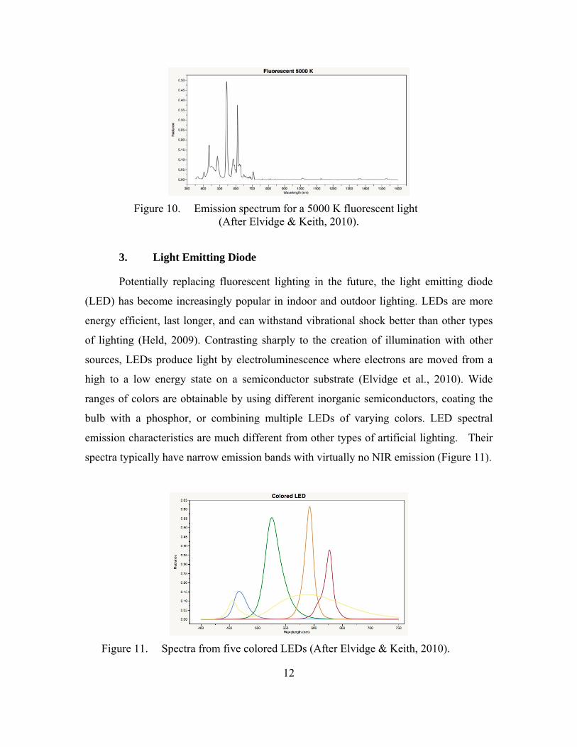
Figure 10. Emission spectrum for a 5000 K fluorescent light (After Elvidge & Keith, 2010).

3. Light Emitting Diode

Potentially replacing fluorescent lighting in the future, the light emitting diode

(LED) has become increasingly popular in indoor and outdoor lighting. LEDs are more

energy efficient, last longer, and can withstand vibrational shock better than other types

of lighting (Held, 2009). Contrasting sharply to the creation of illumination with other

sources, LEDs produce light by electroluminescence where electrons are moved from a

high to a low energy state on a semiconductor substrate (Elvidge et al., 2010). Wide

ranges of colors are obtainable by using different inorganic semiconductors, coating the

bulb with a phosphor, or combining multiple LEDs of varying colors. LED spectral

emission characteristics are much different from other types of artificial lighting. Their

spectra typically have narrow emission bands with virtually no NIR emission (Figure 11).

Figure 11. Spectra from five colored LEDs (After Elvidge & Keith, 2010).

13

C. OPTICAL REMOTE SENSING

Optical remote sensing systems record electromagnetic energy in wavelengths

that can be reflected and refracted with lenses and mirrors. The portion of the EMS that is

typically associated with these systems ranges from ultraviolet (UV) to thermal infrared

(TIR). Optical systems that typically produce spectral imagery express recorded energy in

digital numbers (DN). An image DN can also be referred to as the recorded brightness

level. The radiometric resolution or dynamic range of a sensor’s detector determines the

levels of brightness that can be recorded. By measuring the brightness of a pixel across

many wavelengths, it is possible to identify a material when the spectral properties of that

material are previously known. A subset of optical remote sensing, multispectral and

hyperspectral imaging provide the tools necessary for material identification.

1. Multispectral Imaging (MSI)

MSI is characterized as recording energy in tens of spectral bands (Richards &

Jia, 2006). In general, MSI systems utilize wide (~100 nm) spectral bandwidths that

range from visible to infrared wavelengths. The wavelengths can be separated by filters

as well as employing detectors that are sensitive to different regions of the EMS. A

device as simple as the camera on a cell phone can be considered a multispectral imager

with three spectral bands (Red, Green, Blue). There are a wide variety of statistically

based methods for analysis of MSI data, but they can also be analyzed to some degree

using MSI spectral signatures.

2. Hyperspectral Imaging (HSI)

Imaging spectrometry, sometimes referred to as hyperspectral imaging or HSI, is

the simultaneous acquisition of images in many narrow, contiguous spectral bands (Goetz

et al., 1985). Each spatial element in the image contains a relatively high spectral

resolution spectrum of energy corresponding to the spectral range of the sensor. The

power of HSI comes from the ability to identify materials by their specific spectral

reflectance or emission signatures. Through laboratory or field measurements, the

spectral signatures of many materials are well known and may be contained in spectral

libraries. Matching the HSI spectrum to a corresponding library spectrum allows

14

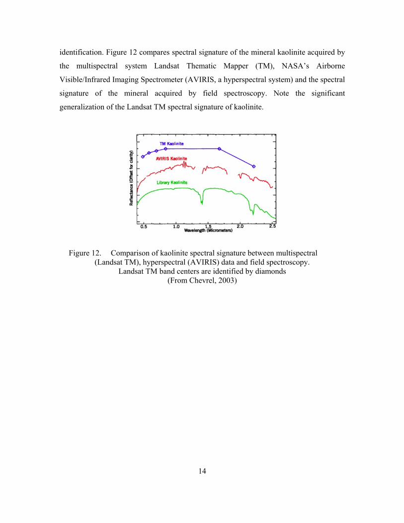
identification. Figure 12 compares spectral signature of the mineral kaolinite acquired by

the multispectral system Landsat Thematic Mapper (TM), NASA’s Airborne

Visible/Infrared Imaging Spectrometer (AVIRIS, a hyperspectral system) and the spectral

signature of the mineral acquired by field spectroscopy. Note the significant

generalization of the Landsat TM spectral signature of kaolinite.

Figure 12. Comparison of kaolinite spectral signature between multispectral (Landsat TM), hyperspectral (AVIRIS) data and field spectroscopy.

Landsat TM band centers are identified by diamonds (From Chevrel, 2003)

15

III. PREVIOUS NIGHTTIME REMOTE SENSING RESEARCH

For decades, the Defense Meteorological Satellite Program (DMSP) Operational

Linescan System (OLS) has been the source of data for much of the night-lights remote

sensing products. DMSP-OLS proved to be a valuable tool to map stable emissions of

cities, towns and industrial sites on a global scale (Elvidge et al., 1997). Recent

advancements in technology have allowed for mapping nocturnal emission sources at a

much higher spatial and spectral resolution than what was achieved with DMSP-OLS.

Research suggests that hyperspectral remote sensing systems can provide the

spectral/spatial resolution needed to achieve identification of lighting by type.

A. DMSP CAPABILITIES AND EXAMPLES

DMSP originated in the mid-1960s as a U.S. Air Force meteorological program

designed to collect worldwide cloud cover on a daily basis (Kramer, 1994). The DMSP

satellite is in a sun-synchronous low Earth orbit with a mean altitude of 833 km where

global coverage is obtained every 24 hours. There have been several upgrades to DMSP

since the program’s creation. The latest Block-5D series upgrade includes the Operational

Linescan System (OLS) (Doll, 2008).

The DMSP-OLS is an oscillating scan radiometer that collects global daytime and

nighttime imagery across 2 spectral bands, visible and thermal infrared (VIS and TIR)

(Elvidge et al., 1997). The visible band (0.5 to 0.9 μm) uses a photomultiplier tube (PMT)

system to intensify the received signal for the detection of clouds at night using

moonlight. The implementation of the PMT system allowed for an unintentional ability to

detect city lights, gas flares, and fires at radiances as low as 109 watts/cm2/sr/μm.

Although the ability of DMSP-OLS to map city lights has been known since the

1970s, the early night-time mapping products were derived from analog data (film).

Elvidge et al. (1997) presented the first method for mapping stable city lights using

digital data from the DMSP-OLS. The results demonstrated that the presence of clouds

can either obscure or diffuse the VNIR light emission from Earth’s surface. The digital

16

method uses a large number of orbits, use of a local background for VNIR emission

source detection, and screening for cloud cover to determine stable light emission from

cities of the United States (Figure 13).

Figure 13. Stable city lights of the United States from DMSP (From Elvidge, et al., 1997)

DMSP-OLS lacks the ability to discriminate and identify lighting types due to its

low spatial (2.7 km) and spectral resolution. A more recent mission, the Visible/Infrared

Imager/Radiometer Suite (VIIRS), provides higher spatial (0.742 km) and radiometric

resolution than DMSP-OLS but still lacks the spectral resolution needed for nocturnal

lighting identification (Elvidge et al., 2007). Realizing the shortcomings of DMSP-OLS

and similar systems, Elvidge et al. (2007) proposed a Nightsat mission concept detailing

a satellite system capable of producing a cloud-free global map of lights on an annual

basis. The Nightsat mission concept uses a combination of high-resolution field spectra

of outdoor lighting, moderate resolution color photography from the International Space

Station (ISS), and high-resolution airborne imagery to define the spatial, spectral, and

17

detection limit options for a future Nightsat mission. The resulting analysis suggests a

sensor having 3 to 5 spectral bands with minimal overlap to enable quantitative

applications for detecting lighting by type.

B. ISS CITIES AT NIGHT

Astronauts aboard the International Space Station (ISS) have provided over

1.5 million digital images of Earth that are freely available through NASA’s “Gateway to

Astronaut Photography of Earth” repository (http://eol.jsc.nasa.gov). Through an optical

quality porthole, astronauts capture digital imagery using handheld Digital Single-Lens

Reflex (DSLR) cameras. A portion of the imagery collected is of major cities at night.

Like many of the space-based optical remote sensing satellites, the ISS is in a low Earth

orbit with a perigee and apogee of around 402 km. The ISS’s orbital altitude allows

capture of higher spatial resolution images than either DMSP or VIIRS. As a remote

sensing platform, the ISS is unique in that new technology can be brought on board when

new missions carrying cargo or crewmembers dock with the ISS.

Early astronauts’ attempts to photograph cities at night often produced blurred

imagery due to the velocity of the ISS and long exposure times needed (Doll, 2008). In

late 2002 through early 2003, astronaut Don Pettit, from ISS Expedition 6, substantially

improved the image quality of photos taken at night by building and installing a tracking

device to compensate for the ISS’s orbital motion (Evans & Stefanov, 2008). By utilizing

Pettit’s tracker, crisp and clear nighttime imagery were obtainable at an estimated spatial

resolution of 60 meters. From late 2007 through early 2008, Flight Engineer Dan Tani of

Expedition 16 extended Pettit’s night photography techniques and acquired images of

cities at night using a 400 mm lens corresponding to an estimated ground resolution of

less than 10 meters (Figure 14).

18

Figure 14. DSLR image of Long Beach, California acquired from the ISS. Orange sodium vapor lights illuminate the port facilities.

Image ISS016-E-27162 taken on February 4, 2008 using a 400 mm lens (From Evans & Stefanov, 2008)

C. SPECTRAL MODELING USING HIGH RESOLUTION LABORATORY MEASUREMENTS

Elvidge et al. (2010) examined the optimal spectral bands for the identification of

lighting types and estimation of four major indices of lighting efficiency. High-resolution

emission spectra of 43 different lamps were collected in order to simulate radiances in

eight spectral bands based on Landsat TM and the human eye photoreceptor bands. This

research recognizes the high cost of building and operating a hyperspectral sensor having

detection limits optimal for observation of night-lights and suggests the broad spectral

bands needed for an alternative instrument.

Using an Analytical Spectral Devices (ASD), Inc. FieldSpec 3 spectroradiometer,

emission spectra were collected from 350 to 2500 nm for nine major types of lamps used

worldwide. The spectra were processed to simulate spectral bands by multiplying the

radiance at each wavelength by the spectral bands response and then summing the results.

The resulting simulated broad bands are based on spectral functions from 5 Landsat TM

bands and 3 human photoreceptor bands.

19

Discriminant analysis using the JMP statistical package was performed in order to

analyze the simulated spectral bands ability to discriminate lighting types. The results

show that Landsat TM visible bands with a slight modification to the near infrared (NIR)

band performed nearly as well as the spectroradiometer data although there was

confusion between white light emitting diodes (LEDs) and fluorescent lamps. The human

photoreceptor bands did not perform well. This research also shows that there does not

appear to be any great value in using spectral bands beyond 1000 nm when distinguishing

lighting types. In addition, it was found that the inclusion of at least one NIR band proved

useful to distinguish incandescent sources from other lighting types.

D. HYPERSPECTRAL IMAGING

1. AVIRIS

To further explore the remote sensing of nocturnal lighting, Elvidge & Green

(2004) analyzed high and low altitude nighttime AVIRIS data over Los Angeles,

California, and Las Vegas, Nevada. Low altitude AVIRIS data were collected over the

central area of Las Vegas, Nevada, at 6:35 pm on October 4th, 1998. The AVIRIS sensor

was flown on a Twin Otter aircraft at an altitude of 12,500 feet above sea level (ASL)

corresponding to an approximate 3 m spatial resolution. In addition, high altitude

AVIRIS data were collected over Los Angeles, California, in 2003 with a spatial

resolution of 20 m. In both AVIRIS datasets, the total radiance was obtained by summing

all of the AVIRIS channels in the flight line to produce an aggregate spectrum. In the Las

Vegas dataset, the aggregate spectrum exhibited features found in mercury and sodium

vapor outdoor lighting. The aggregate spectrum of the Los Angeles dataset showed none

of the emission lines that characterize most outdoor lighting. A small number of pixels

had detected emissions from heavily lit automobile dealerships, gravel quarries, and gas

flares in oil refineries.

The resulting analysis showed that the AVIRIS sensor at both high and low

altitude is capable of detecting bright lights pointed directly into the sky as well as minor

gas flares in the shortwave infrared (SWIR) region. The spectral signatures of AVIRIS-

detected nocturnal lighting and gas flares were found to have sufficient detail to make the

20

identification of lighting type or the composition of burning gas(es) feasible. The overall

assessment, however, was that AVIRIS (as of 2003) did not have detection limits low

enough to detect the bright emission lines of general street and outdoor lighting.

2. ProSpecTIR VS Imaging Spectrometer

Kruse & Elvidge (2011) focused on assessing the capability of hyperspectral

remote sensing to identify and map nocturnal lighting located in Las Vegas, Nevada. The

authors were able to map select artificial light sources using data from both the

ProSpecTIR-VS imaging spectrometer and a NOAA spectral library of lighting types.

The ProSpecTIR-VS imaging sensor produces a 360-band hypercube over a

spectral range from 0.4 to 2.45 micrometers with a 5 nm spectral resolution. Covering

approximately the same spectral range, the NOAA spectral library contains 43 different

spectral signatures across 9 major lighting types at 1 nm spectral resolution. Pixel

signatures from the hyperspectral image were interactively extracted and visually

compared to signatures from the spectral library.

A binary encoding supervised classification was used to carry out light

identification on a pixel-by-pixel basis. The binary encoding classification is

a spectral matching algorithm that compares each image spectrum in the imaging

spectrometer dataset to each spectrum in the spectral library. Only 190 spectral bands

(0.4–1.4 micrometers) were needed to classify lighting types since the spectral signatures

of lighting types in the spectral library show that little information can be useful beyond

1.4 micrometers. To help locate the origin of specific spectral signatures, the ProSpecTIR

image was overlain with a ~0.6-meter spatial resolution panchromatic Quickbird image

corresponding to the same area of interest. The resulting map of lighting types shows

metal halide lights, two colors of neon (red and blue), and high-pressure sodium light

sources spatially associated with their ground locations (Figure 15).

21

Figure 15. Classification of night lighting for selected lighting types using binary encoding. Classification map overlain on Quickbird image to

illustrate building association with lighting type (From Kruse & Elvidge 2011).

To build upon the previous nighttime remote sensing research, it would be useful

to explore the possibility of identifying city lights by type using MSI. The Las Vegas

ProSpecTIR data were used as the basis in this research for assessing the accuracy of

nocturnal lighting identification by means of multispectral imagery.

22


23

IV. DATA AND METHODS

A. SITE

Widely known as a popular resort and gambling destination, the city of Las

Vegas, Nevada is arguably one of the brightest cities on Earth and thus was selected for

this study. Central to the city, the “Strip” offers a wide variety of lighting types and

intensities. In order to attract the eye of patrons, a particularly heavy emphasis is placed

on illuminating every visible aspect of many of the buildings that currently operate within

the strip. In addition, the 24-hour operation of most businesses in this area ensures an

ample amount of available light during all hours of the night. A discussion of the lights of

Las Vegas is not complete without mentioning the Luxor Sky Beam. The strongest beam

in the world at 43.2 billion candlepower, the Luxor Sky Beam is comprised of 39 xenon

lamps directed straight into the sky by computer designed curved mirrors (Attractions:

Highlights, 2012). Figure 16 illustrates the wide variety of lighting in Las Vegas.

Figure 16. Oblique photo of the Las Vegas Strip at night (Courtesy of PDphoto.org)

24

B. DATA

Depending on the type of analysis to be performed, there are several

considerations that need to be addressed when collecting nighttime data. For a global

inventory of lighting, a sensor that has a high revisit rate and moderate spatial resolution

is needed. If lighting discrimination and identification is the goal, the high spectral and

spatial resolution that HSI provides is desirable. For the purposes of this research, both

hyperspectral and multispectral data were acquired.

1. ProSpecTIR-VS Imaging Spectrometer

The ProSpecTIR-VS Dual Sensor is a high performance aerial hyperspectral

imaging system operated by SpecTIR, LLC (spectir.com) that acquires both VNIR and

SWIR data simultaneously. The dual system combines the AISA’s Hawk (VNIR) and

Eagle (SWIR) imaging sensors where both imagers are co-aligned to correspond to the

same swath on the ground as well as providing a single data cube with a spectral range

from 400 to 2450 nm. In addition, the Hawk lens can be adjusted to match the ground

pixel size to that of the Eagle sensor. Table 1 summarizes the specifications of the

ProSpecTIR Dual sensor setup.

Table 1. Operational characteristics and imaging modes of ProSpecTIR-VS Dual Sensor system (SpecTIR Product Line).

25

A 360-band hyperspectral data cube was collected using the ProSpecTIR-VS

system on July 28, 2009 at 10:55 PM over the Las Vegas strip. The altitude of the collect

was approximately 1778 m corresponding to a ground sample distance (GSD) of 1.2 m.

SpecTIR LLC calibrated the HSI datacube to radiance using dark current correction,

array normalization and radiometric calibration (Kruse & Elvidge, 2010). The entire

image is 320 lines by 11778 samples (Figure 17).

Figure 17. True color (650, 550, 450 nm as RGB) ProSpecTIR dataset in five segments. Image segmented along numbered labels from left to right.

26

2. International Space Station DSLR Imagery

The DSLR camera used to acquire the multispectral ISS image used in this study

was a Nikon D3S (Figure 18). The D3S features a 36.0 mm by 23.9 mm complimentary

metal-oxide-semiconductor (CMOS) sensor that produces a total pixel count of

12.87 million. International Organization for Standardization (ISO) sensitivity settings

can range from 200 to 12800.

Figure 18. Nikon D3S DSLR camera assembly (Nikon D3S Tech Specs)

The image selected for this research was acquired during ISS Expedition 26 and

captures the entire city of Las Vegas, Nevada (Figure 19). A RAW image format was

requested preserve image quality. Table 2 provides a summary of the camera settings

during the time of collection. The camera settings indicate that automatic white balance

and image compression were used during collection. Nonetheless, the ISS image clearly

shows linear street patterns predominantly lit by sodium vapor lamps as well as the

characteristic blue/green color of mercury vapor lamps on the left of the city center. The

Las Vegas strip is well defined by the brightest area (Figure 19 center) of the image.

27

Table 2. Nikon D3S Camera settings for ISS026E006241.nef

Figure 19. ISS026E006241.nef acquired from NASA’s Gateway to Astronaut Photography of Earth (http://www.eol.jsc.nasa.gov)

28

3. Spectral Library of Lighting

Elvidge et al. (2010) produced a spectral library of emission spectra for various

light sources that were collected in a laboratory setting (Figure 20). The instrument used

for collection was an ASD, Inc. FieldSpec 3 spectroradiometer that had been

radiometrically calibrated and operating in radiance mode where individual spectra

are reported in watts m-2 sr-1 μm-1. Post processing yields spectra with 1 nm increments

from 350 to 2,500 nm. The library is available through National Oceanic and

Atmospheric Administration’s (NOAA) Earth Observation Group website

(http://www.ngdc.noaa.gov/dmsp/spectra.html).

Figure 20. Comparison of selected emission spectra in radiance (0.4 to 1.4 micrometers) for selected lighting types. Spectral signatures from the NOAA lighting spectral library (From Kruse & Elvidge, 2010)

29

C. METHODS

Image processing of various types is required to be performed on each dataset

before image analysis can be accomplished. The following summarizes the methods used

for each dataset for this research.

1. Spectral Library Resampling

To directly compare the spectral signatures from image pixels and library spectra,

the spectral library must be resampled to the response of the particular sensor being used.

In the approach used for this research, because the spectral response of each instrument

was known, the spectral library was resampled to the appropriate instrument’s response

by multiplying the library by the response value for a given wavelength. The resulting

spectral library has the same number of samples for each lighting type as the number of

spectral bands of the instrument.

a. Resample to Nikon D3 Response

Spectral response data for the Nikon D3S camera remains unpublished.

Assumed to have similar detector characteristics to the Nikon D3S, response data for the

purposes of this study was acquired for the Nikon D3 camera (Cao et al., 2009). The

spectral response of the Nikon D3 detector is reported in normalized spectrum intensity

ranging from 0 to 1 for the red, green, and blue channels (Figure 21). Response data was

converted from an ASCII format to a spectral library as a resampling input. Figure 22

shows the resulting resampled spectral library of select lighting types.

30

Figure 21. Spectral response for Nikon D3 DSLR camera red, green and blue channels recorded at 5 nm intervals (After Cao et al., 2009)

Figure 22. Spectral library of selected lighting types resampled to match spectral response of Nikon D3 DSLR camera. Camera signatures of fluorescent,

mercury vapor, metal halide, high-pressure sodium, and red neon are shown.

b. Resample to Worldview 2 Response

In orbit since October 2009, DigitalGlobe’s WorldView-2 (WV-2)

satellite sensor provides imagery in 8 spectral bands as well as a high spatial resolution

panchromatic band (Spectral Response for DigitalGlobe Earth Imaging Instruments,

31

2011) (Figure 23). While not currently configured for nighttime imaging, the WV-2

spectral band responses provide a model for existing and possible future MSI sensors to

help test probable nighttime imaging capabilities. Therefore, the NOAA spectral library

of lighting types was resampled to the 8 multispectral bands of the WV-2 sensor response

to help prototype the performance of these systems (Figure 24 left). In addition to the 8-

band mode, additional spectral libraries were created for 6-band (coastal blue, blue,

green, yellow, red and red edge) and 4-band (blue, green, red, and NIR1) modes to test

those alternate configurations (Figure 24 middle and right).

Figure 23. Spectral response of the WorldView-2 satellite (From http://www.digitalglobe.com/downloads/DigitalGlobe_Spectral_Response.pdf)

32

Figure 24. Spectral library of selected lighting types resampled to the WorldView-2 spectral response for the 8-band (left), 6-band (middle), and

4-band (right) modes.

2. Nikon D3S DSLR Camera Imagery

a. RAW Conversion

A RAW image is the highest quality format that the Nikon D3S can

provide. Images captured in the RAW format provide high radiometric resolution at 12 or

14 bits either compressed or uncompressed. Because Nikon’s Electronic Format (NEF)

RAW images are not readily ingestible by remote sensing software, a conversion to an

appropriate but lossless format is needed. The ISS image was converted from the RAW

format to a 16-bit TIFF file. No adjustments to the image were made during conversion.

b. Image Registration and Spatial Subsetting

A previously georeferenced ISS image with the same serial number

as the RAW image used for this research was obtained from NOAA

(http://www.ngdc.noaa.gov/dmsp/ISS_Las_Vegas.html). Ground control points (GCPs)

were selected and used as input to perform image to image registration with a 1st order

33

polynomial nearest neighbor method. The resulting map referenced ISS image yields

pixels with a spatial resolution of 20 m. A spatial subset was also performed on the

georeferenced results to remove border areas that were introduced by the image

registration process.

c. Saturation and Dark Pixel Masking

When the DN of a pixel is at or above the radiometric threshold of a

sensor, that pixel is considered saturated and should be ignored when performing image

analysis. Saturated pixels provide little information in spectral studies because the actual

brightness of the pixel is unobtainable. Figure 25 shows areas of saturation primarily

along the Las Vegas strip. Since the aim of this research is to classify pixels exhibiting

light emission, dark pixels found in the image were also ignored. Image statistics suggest

that the darkest pixels have DN values between 0 and 10,000 on average for all three

bands. Two criteria determined whether a pixel will be ignored, (1) any pixel that had a

DN at the saturation threshold value regardless of spectral band and (2) pixels with DNs

between 0 and 10,000.

Figure 25. Masked pixels of saturated areas (red) in the ISS image. Saturation occurs primarily along the Las Vegas Strip.

34

d. Supervised Classification

A spectral information divergence (SID) supervised classification was performed

using the Nikon D3 resampled spectral library of lighting type as reference spectra. The

SID method treats each pixel spectrum as a random variable and defines a probability

distribution from its spectral histogram. The spectral similarity between pixel and

reference spectra is then measured by the discrepancy of probabilistic behaviors between

them (Chang, 1999). The SID method is calculated in the following manner: let x

represent a given multispectral/hyperspectral pixel vector and y a given reference vector

x (x1,..., xL )T (4)

and

y (y1,..., yL )T (5)

where each component xl is a pixel of band image Bl and each yl is a sample from the

reference data. Then x and y can be modeled as a random variable by defining an

appropriate probability distribution. Assuming each x and y component are nonnegative,

both are then normalized to the range [0,1] by

pj x j / xll1

L

(6)

and

qj yj / xll1

L

(7)

so that

1{ }Ll lp p (8)

and

1{ }Ll lq q (9)

where p and q the desired probability vectors for pixel vector x and reference vector y,

respectively. Using p and q, the SID method is defined by

SID(x, y) D(x || y) D(y || x) (10)

where

D(x || y) pll1

L

log(pl / ql ) (11)

35

and

D(y || x) ql log(ql / pl )l1

L

(12)

Like most spectral mapping methods, the SID method assumes that the data to be

classified is already in radiance or reflectance. Unfortunately, the ISS imagery used for

this study could not be converted to radiance units due to the lack of appropriate

conversion parameters and/or a published method to do so. This limitation is somewhat

overcome since each pixel and reference vector is normalized with a range of 0 to 1

during processing in Equations 6 and 7.

3. ProSpecTIR Imaging Spectrometer Data

a. Image Registration

To provide a ground truth image for the ISS nocturnal lighting

classification, the full ProSpecTIR imagery was map referenced by performing image

registration using a geometry lookup table (GLT) file. The GLT file is produced utilizing

aircraft altitude information, inertial navigation details, and GPS collected concurrently

with image acquisition and contains detailed acquisition information that allows model-

based geometric map registration using platform geometry. The GLT provides the map-

referenced coordinates for every image pixel in the dataset, which are then used to

geocorrect the data to match a specified map projection and pixel size.

b. Spectral and Spatial Subsetting

Because the bulk of outdoor lighting emission features occur between

0.4 and 1.0 μm, a spectral subset of the ProSpecTIR imagery was created to bring the

number of spectral bands down to 128 (0.4 to 1.0 μm) from the original 360. The selected

spectral range of this subset also benefits from being well outside major atmospheric

water absorption bands (approx. 1.4 and 1.8 μm). In addition, a spatial subset of the same

dataset was created to eliminate areas of low illumination. Both pre-processing functions

allow for a reduced computational time for subsequent processing.

36

c. Dark Pixel Masking

A mask was created for the ProSpecTIR imagery to ignore areas that

contain zero emission features. Because the majority of the image is essentially dark, the

maximum of all of the mean radiance values across all spectral bands is good indicator of

dark areas and was used as a masking threshold value. This ensures that the classifier to

be used only examines pixels with emission above the mean of the darkest radiance

values for all spectral bands.

d. Supervised Classification

The SID classification method was performed on all ProSpecTIR datasets

using spectral signatures of selected lighting types from the NOAA spectral library as

reference. Used as a basis for evaluation of the ISS nocturnal lighting classification, the

entire hyperspectral image was validated using spatial/spectral data browsing and visual

inspection of emission lines found in the ProSpecTIR data and spectral library. Regions

of interest (ROIs) were created for image pixels exhibiting spectral emission

characteristics matching those found in the NOAA spectral library and these were then

used in the SID classification.

37

V. RESULTS

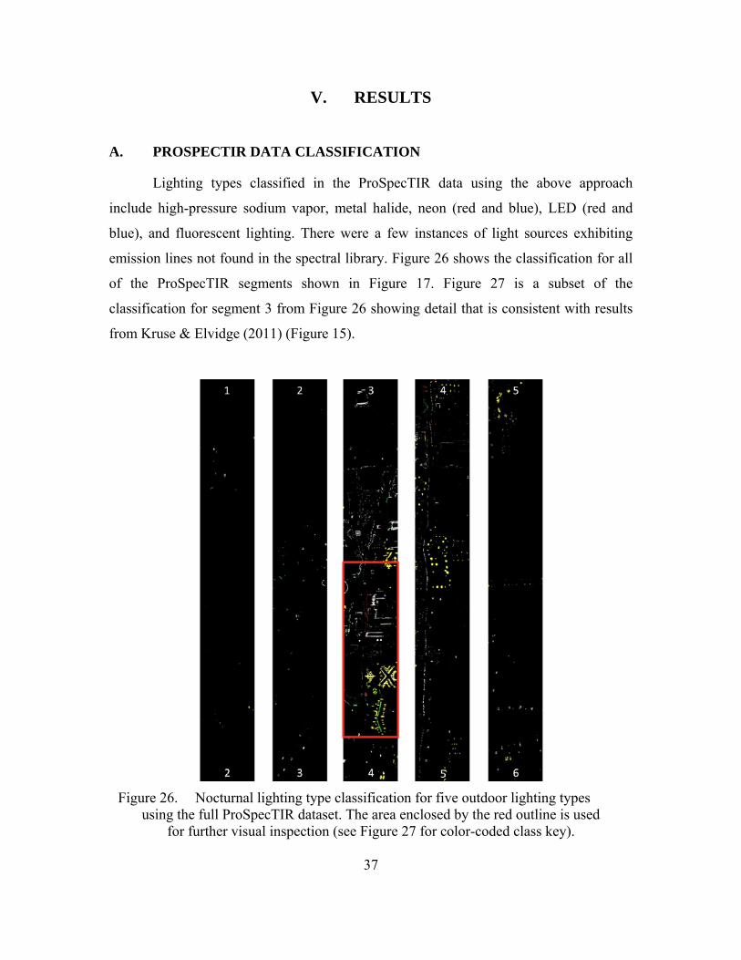
A. PROSPECTIR DATA CLASSIFICATION

Lighting types classified in the ProSpecTIR data using the above approach

include high-pressure sodium vapor, metal halide, neon (red and blue), LED (red and

blue), and fluorescent lighting. There were a few instances of light sources exhibiting

emission lines not found in the spectral library. Figure 26 shows the classification for all

of the ProSpecTIR segments shown in Figure 17. Figure 27 is a subset of the

classification for segment 3 from Figure 26 showing detail that is consistent with results

from Kruse & Elvidge (2011) (Figure 15).

Figure 26. Nocturnal lighting type classification for five outdoor lighting types using the full ProSpecTIR dataset. The area enclosed by the red outline is used

for further visual inspection (see Figure 27 for color-coded class key).

38

Figure 27. Georeferenced nocturnal lighting type classification for five outdoor lighting types. Due to the spatial size of the dataset, only a small portion of the full

classification is shown (part of segment 3 from Figure 26).

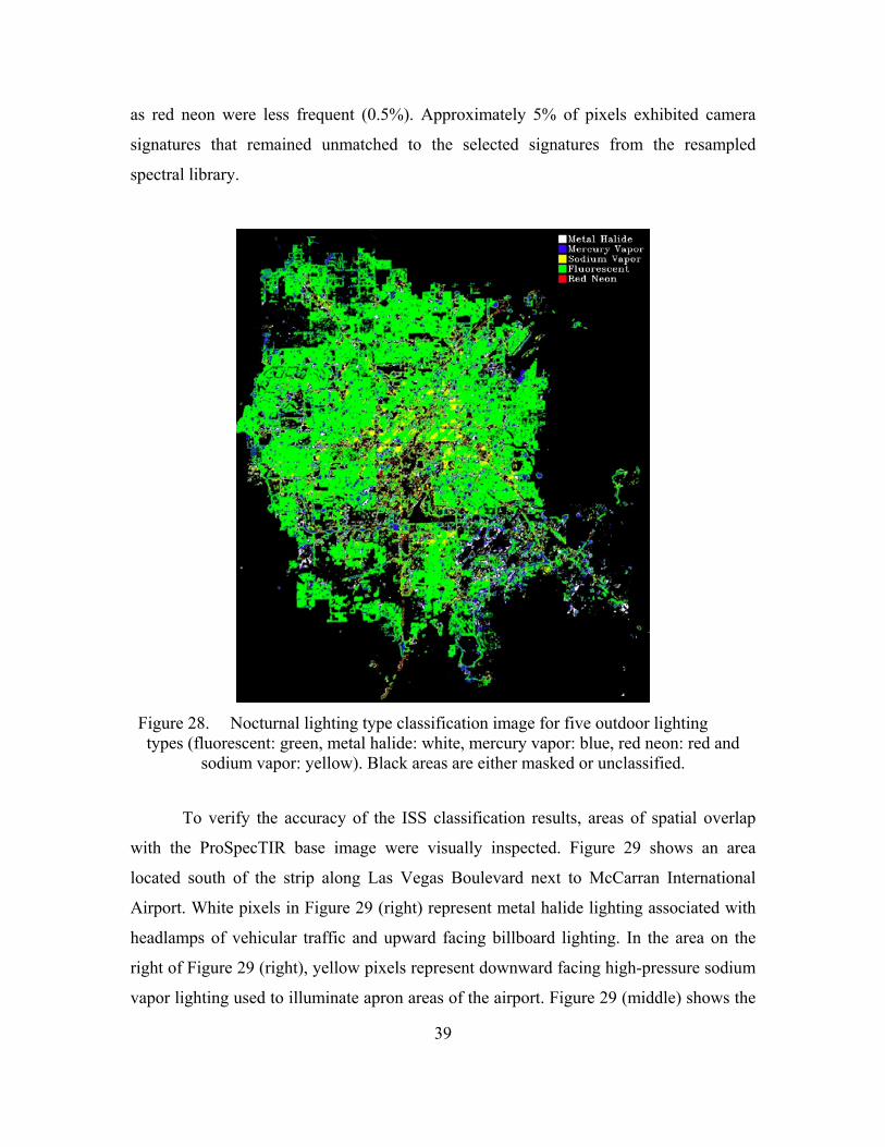
B. ISS LIGHTING TYPE CLASSIFICATION

The ISS image was classified using the SID mapping method with selected

resampled library spectral signatures of lighting types that were frequently found in the

ProSpecTIR base classification (Figures 27 and 28). Figure 28 and supporting statistics

illustrate that approximately 24% of pixels in the image map were classified as

fluorescent lighting despite the characteristic orange color of sodium vapor lamps found

across the original ISS image (Figure 19). Mercury vapor, sodium vapor and metal halide

lighting classes each represent between 3% and 5% of the image while pixels classified

39

as red neon were less frequent (0.5%). Approximately 5% of pixels exhibited camera

signatures that remained unmatched to the selected signatures from the resampled

spectral library.

Figure 28. Nocturnal lighting type classification image for five outdoor lighting types (fluorescent: green, metal halide: white, mercury vapor: blue, red neon: red and

sodium vapor: yellow). Black areas are either masked or unclassified.

To verify the accuracy of the ISS classification results, areas of spatial overlap

with the ProSpecTIR base image were visually inspected. Figure 29 shows an area

located south of the strip along Las Vegas Boulevard next to McCarran International

Airport. White pixels in Figure 29 (right) represent metal halide lighting associated with

headlamps of vehicular traffic and upward facing billboard lighting. In the area on the

right of Figure 29 (right), yellow pixels represent downward facing high-pressure sodium

vapor lighting used to illuminate apron areas of the airport. Figure 29 (middle) shows the

40

same area in the ISS classification. A comparison of both classification images shows

that the ISS classification produced much different results from the base classification.

An examination of the camera signatures in the original ISS image revealed two

possible reasons for the differences; (1) camera signatures associated with known

lighting do not accurately match the resampled library spectral signatures for the same

lighting type, and (2) camera signatures vary highly as distance increases from pixels

associated with the lighting source.

Figure 29. Comparison of original ISS image (A, left), classified ISS image (B, middle) and classified ProSpecTIR image (C, right) for a selected area.

Figure 30 shows spectral plots for known metal halide (left) and high-pressure

sodium vapor lighting (right) for selected pixels in the ISS image before classification.

ISS camera signatures for pixels associated metal halide and high-pressure sodium vapor

do not match the general shape of library spectra for these lighting types. Although this

area has been shown to exhibit mostly metal halide and high-pressure sodium vapor

lighting, the ISS classification suggests that there are many more lighting types present.

Although an area that is principally lit by one type of light, the camera signature signature

will change when moving from bright pixels to darker pixels of the same lighting type.

41

Linear profile transects and spatial/spectral browsing of camera signatures for high-

pressure sodium vapor lit areas confirm that camera signatures vary highly when the

distance from the brightest pixels increases. This phenomenon is consistent for multiple

lighting types throughout the whole ISS image.

Figure 30. Camera signatures of known metal halide (left) and high-pressure sodium lighting (right) compared to their corresponding

library spectral signatures.

C. 8-, 6-, AND 4-BAND WV-2 MODELED CLASSIFICATION

For this study, the 128-band ProSpecTIR classification is considered ground truth

for nocturnal lighting of Las Vegas, NV and will be referred to as such throughout the

results. A probability threshold of 0.2 was used for the 8- and 6-band images while a

0.05 threshold was used for the 4-band image. Figures 31 and 32 show selected areas of

the nocturnal lighting classification results using the ground truth, 8-, 6- and 4-band WV-

2 modeled images.

42

Figure 31. Comparison of nocturnal lighting classifications using a spectral subset (0.4 to 1.0 mm) of the ProSpecTIR dataset and three WV-2 modeled multispectral

images. Gray areas are masked pixels and black areas are unclassified pixels exhibiting emission features. Note same classification key and colors apply to all three images.

43

Figure 32. Comparison of ground truth, 8-band, 6-band, and 4-band classification images for area ‘A’

Figure 32 shows a close up of the area labeled “A” in Figure 31 (left) that refers

to a linear series of lights associated with “Bill’s Gambling Hall.” White pixels located

in the vicinity of the building exhibited spectral emission lines that matched those of

metal halide lamps. All three WV-2 modeled images show slight confusion between

metal halide and other gaseous discharge lighting. The 8- and 6-band classifications show

a mix of both fluorescent and high-pressure sodium vapor lighting while the 4-band

classification confused these lights almost exclusively with high-pressure sodium vapor

44

lights. Confusion between fluorescent and high-pressure sodium vapor is also exhibited

in other areas of metal halide lighting found in the ground truth classification. Red neon

outside of the building mapped well in the 8-band classification. The 8- and 6-band

classifications correctly mapped the low radiance metal halide light to the west and east

of the building. The metal halide light “streaking” appears to be a lens artifact possibly

induced by the imaging spectrometer as it imaged directly over the lighting. Figure 33

shows an example for selected high-pressure sodium vapor lighting.

Figure 33. Comparison of ground truth, 8-band, 6-band, and 4-band classification images for area ‘B’

The area labeled “B” (Figure 31 left) points to high-pressure sodium vapor

lighting on the Eiffel Tower replica in front of the Paris hotel. This is another example of

the spectral similarity of fluorescent and high-pressure sodium lighting when resampled

to a lower spectral resolution. A pattern becomes apparent where pixels between the

bright sodium vapor lighting (yellow) in the ground truth were incorrectly classified as

fluorescent lighting (green) in the multispectral classifications (Figure 33).

Area “C” refers to the red and blue neon lighting located on the Montgolfier

balloon structure and a series of blue LED lights south of the balloon (Figure 34). The

ground truth classification shows that the balloon is surrounded on all sides by red neon

lighting with blue neon lighting on the top of the structure. Although both the 8- and 6-

band WV-2 modeled classifications mapped the red and blue neon lighting on the

Montgolfier Balloon, it was not to the extent of what the ground truth mapped. The area

between the two colors of neon lighting was found to exhibit emission lines not found in

the spectral library (yellow neon) (Figure 35). The WV-2 classifications show that the

45

yellow neon lighting was confused with fluorescent, metal halide and high-pressure

sodium. Area “C” is the only location where blue LED lighting was located. The 8- and

6-band classifications mapped blue LED lighting quite well.

Figure 34. Comparison of ground truth, 8-band, 6-band, and 4-band classification images for area ‘C’

46

Figure 35. Montgolfier Balloon structure showing three colors of neon lighting. (Photo courtesy of http://www.lonelyplanet.com/usa/great-plains/travel-tips-

and-articles/76005).

C. CONFUSION MATRICES

To show the accuracy of classification for the WV-2 modeled images, confusion

matrices were created using the 128-band ProSpecTIR-VS classification as ground truth.

The confusion matrices report the overall accuracy, kappa coefficient, percentages of

classification agreement, omission/commission errors and producer/user errors. The

overall accuracy is calculated by summing the number of pixels classified correctly and

then dividing by the total number of pixels (Congalton, 1990). The kappa coefficient (k)

is a discrete multivariate technique that offers an additional measure of agreement or

accuracy. The kappa coefficient is computed by

N xii

i1

r

xii1

n

x i

N 2 i1

r

(xixi ) (13)

where N is the total number of pixels in all the ground truth classes, r is the number of

rows in the matrix, and xii is the number of observations in row i and column i, xi+ and x+i

are the marginal totals of row i and column i, respectively. The producer’s accuracy

47

refers the probability of a reference pixel being correctly classified while the user’s

accuracy is the probability that a pixel classified on the map is actually that class.

Percentages of class agreement (producer’s accuracy) are reported along the diagonal

from top left to bottom right and are highlighted in bold.

1. 8-Band Confusion Matrix

Table 3 shows the confusion matrix using the ground truth image and the 8-band

classification map. An overall accuracy of approximately 59% and a kappa statistic of

0.433 suggest a moderate classification performance for all lighting types mapped. On the

other hand, a review of the producer and user accuracies show that the neon (red and

blue) and blue LED classes mapped very well with 8-bands. Conversely, the red LED

class had zero agreement with the ground truth image and went completely classified as

the red neon class. Sodium vapor, metal halide, fluorescent and blue neon lighting classes

showed the next best agreement percentages between approximately 41% and

91% although confusion between them is apparent.

Table 3. Classification matrix using the ground truth and 8-band classifications of nocturnal lighting.

48



classification map. The reported overall accuracy is higher than that from the 8-band

classification although the kappa coefficient is slightly lower. Again, the red neon and

blue LED class performed well with 100% agreement and high producer/user accuracies.

The metal halide and blue neon classes had slightly higher percentages for the 6-band

classification when compared to the same values for the 8-band classification. A review

of Figure 24 provides some insight on why the gaseous discharge classes performed

rather poorly when compared to other classes. Metal halide, fluorescent and sodium

vapor lighting have very similar spectral signatures across the 8-, 6-, and 4 band spectral

libraries.




classification map. At approximately 23%, the overall accuracy of the 4-band

classification was significantly lower than the 6- or 8-band classification accuracies. A

very low kappa statistic indicates only slight agreement for all lighting classes. Blue

neon shows a 100% class agreement although the user accuracy reveals that only 39.85%

49

of pixels labeled as this class are actually blue neon. The sodium vapor, metal halide, and

fluorescent classes show higher agreement within that set of classes outside of the

diagonal. Additionally, increased confusion between similarly colored LED and neon

classes is introduced with the 4-band configuration.


50


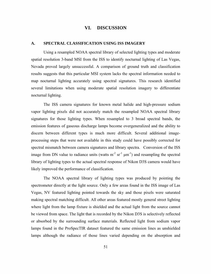
51

VI. DISCUSSION

A. SPECTRAL CLASSIFICATION USING ISS IMAGERY

Using a resampled NOAA spectral library of selected lighting types and moderate

spatial resolution 3-band MSI from the ISS to identify nocturnal lighting of Las Vegas,

Nevada proved largely unsuccessful. A comparison of ground truth and classification

results suggests that this particular MSI system lacks the spectral information needed to

map nocturnal lighting accurately using spectral signatures. This research identified

several limitations when using moderate spatial resolution imagery to differentiate

nocturnal lighting.

The ISS camera signatures for known metal halide and high-pressure sodium

vapor lighting pixels did not accurately match the resampled NOAA spectral library

signatures for those lighting types. When resampled to 3 broad spectral bands, the

emission features of gaseous discharge lamps become overgeneralized and the ability to

discern between different types is much more difficult. Several additional image-

processing steps that were not available in this study could have possibly corrected for

spectral mismatch between camera signatures and library spectra. Conversion of the ISS

image from DN value to radiance units (watts m-2 sr-1 μm-1) and resampling the spectral

library of lighting types to the actual spectral response of Nikon D3S camera would have

likely improved the performance of classification.

The NOAA spectral library of lighting types was produced by pointing the

spectrometer directly at the light source. Only a few areas found in the ISS image of Las

Vegas, NV featured lighting pointed towards the sky and those pixels were saturated

making spectral matching difficult. All other areas featured mostly general street lighting

where light from the lamp fixture is shielded and the actual light from the source cannot

be viewed from space. The light that is recorded by the Nikon D3S is selectively reflected

or absorbed by the surrounding surface materials. Reflected light from sodium vapor

lamps found in the ProSpecTIR dataset featured the same emission lines as unshielded

lamps although the radiance of those lines varied depending on the absorption and

52

reflection characteristics of that surface. These phenomena would likely produce highly

variable spectral signatures across all lighting types when resampled to only 3 spectral

bands.

At 20 m spatial resolution, light appears to spread much further than at lower

spatial resolutions. At a glance, outdoor lighting appeared to remain continuous

throughout areas of light concentration in the ISS image. The spread of light is much

more concise as seen with the ProSpecTIR imagery at 1.2 m spatial resolution. The ISS

classification revealed that a camera signature varies with distance from the lighting

source. Even if camera signatures associated with the source of lighting were correctly

matched to its reference spectra, the surrounding light would classify as a different

lighting type.

B. SPECTRAL CLASSIFICATION USING WV-2 MODELED IMAGERY

Classification of nocturnal lighting using WV-2 modeled 8-, 6-, and 4-band

subsets provided additional information on the performance of MSI to spectrally

discriminate lighting by type. A previous night-lights study from Elvidge et al. (2010)

suggested that the inclusion of one or more NIR bands could enhance the discrimination

high intensity discharge (HID) lamps from fluorescent lighting. Therefore, the initial

hypothesis for this study was that classification of nighttime lighting using the two NIR

bands from WV-2 would perform much better than the 6 or 4 band configurations for

HID and fluorescent lighting discrimination. In this study, however, utilizing the NIR1

and NIR2 bands from the WV-2 sensor did not provide the additional spectral

information needed to clearly discriminate between the gaseous discharge lighting types

found in Las Vegas, NV when compared to the 6-band configuration.

The SID classification method was shown to be sensitive to areas exhibiting

similar spectral signatures with varying radiance for the WV-2 simulations (Figure 33).

Areas lower in radiance were classified as fluorescent lighting although the spectral

signature remained relatively constant between sources of sodium vapor lighting. The

reason for much of the misclassification is probably due to the close similarity of

fluorescent and sodium vapor lighting spectral signatures when resampled to a lower

53

spectral resolution. Figure 24 shows that the spectral signatures for fluorescent, red LED,

metal halide and sodium vapor lighting all have emission peaks corresponding to the

WV-2 yellow band. Additionally, the SID threshold of 20% used for classification is

likely a key factor for the introduction of spectral confusion between lighting types.

Using a lower threshold would have reduced much of the confusion although many of the

pixels that exhibited emission features would have gone unclassified.

Analysis of confusion matrices shows that the 8- and 6-band nocturnal lighting

classifications using SID performed similarly in overall class agreement and general

mapping ability while the 4-band classification performed somewhat more poorly. A

general pattern exists between all three confusion matrices where groups of similar

lighting types were confused with each other. The SID classifier often confused sodium

vapor, metal halide, and fluorescent lighting classes together across all three WV-2

configurations while similar colored neon and LED confusion became apparent using

only four WV-2 bands.

54


55

VII. CONCLUSION AND RECOMMENDATIONS

Moderate spatial resolution ISS multispectral imagery of Las Vegas, NV was

investigated to determine the potential of accurately mapping nocturnal lighting using a

processed NOAA spectral library of lighting types as reference. Additional MSI research

was conducted using three WV-2 modeled datasets derived from resampled HSI. The

primary limitation of using resampled library spectra of outdoor lighting and space-based

MSI to accurately map nocturnal lighting is the loss of spectral emission features

exhibited by gaseous discharge lighting.

Mapping nocturnal lighting using HSI remains the most accurate method to

differentiate the emission features associated with urban outdoor lighting. Although the

different colors associated with outdoor lighting can be visually delineated in nighttime

ISS imagery from a DSLR camera, the limited spectral information and corresponding

degraded spectral performance of MSI does not allow for accurate lighting type

classification. At 20 m spatial resolution, camera signatures associated with lighting were

found to be highly variable as distance increased from the brightest pixels. This led to an

inaccurate map of nocturnal lighting where one type of light would be classified as

several.

Additional MSI research using three WV-2 multispectral band configurations

demonstrated increased ability to separate lighting types by their spectral signatures. With

8, 6 or 4 spectral bands, accurate discrimination of lighting types remains a daunting task.

MSI sensors having spectral bands similar to WV-2 should be able to map certain types

of artificial lighting quite well (red/blue neon and blue LED) while other types (sodium

vapor, fluorescent, and metal halide) have high spectral similarities when resampled and

would be somewhat difficult to separate.

Numerous opportunities for improvement on this study exist. Future work on this

subject should include collection of nighttime MSI at a higher spatial resolution than 20

meters in order to detect and characterize isolated lighting sources. In addition, it would

be useful to image an area that exhibited all of the lighting types contained in the NOAA

56

spectral library to further research spectral discrimination of more than 5 types.

Incandescent sources were found in the ProSpecTIR imagery but were excluded from

classification due to atmospheric absorption. Mapping incandescent sources would likely

emphasize the utility of using NIR bands to discriminate these from other lighting types.

57

LIST OF REFERENCES

Attractions: Highlights. (2012). Retrieved July 27, 2012, from Luxor: http://www.luxor.com/attractions/attractions_property_highlights.aspx

Campbell, J. B. (1996). Introduction to remote sensing (2nd ed.). New York: Guilford Press.

Cao, F., Guichard, F., Hornung, H., & Masson, L. (2009). Sensor information capacity and spectral sensitivities. SPIE 7250 Proceedings. Digital Photography V, 725006.

Chang, C. I. (1999). Spectral information divergence for hyperspectral image analysis. Geoscience and Remote Sensing Symposium, 1999. IGARSS ‘99 Proceedings. IEEE 1999 International, vol.1, no., 509–511.

Chevrel, S. (2003). Mineo Project Final Report. Retrieved September 21, 2012, from Mineo Project: http://www2.brgm.fr/mineo/final.htm

Cho, K., R. Ito, R., Shimoda, H., & Sakata, T. (1999). Fishing fleet lights and sea surface temperature distribution observed by DMSP/OLS sensor. International Journal of Remote Sensing , 20, 3–9.

Cinzano, P., Falchi, F., Elvidge, C.D., & Baugh, K.E. (2000). The artificial night sky brightness mapped from DMSP Operational Linescan System measurements. Monthly Notices of the Royal Astronomical Society, 318, 641–657.

Congalton, R. G. (1991). A review of assessing the accuracy of classifications of remotely sensed data. Remote Sensing of Environment, 37, 35–46.

Croft, T. (1978). Nighttime images of the earth from space. Scientific American , 239, 68–79.

Doll, C. N. H. (2008). CIESIN thematic guide to night-time light remote sensing and its applications. Palisades, NY: Center for International Earth Science Information Network of Columbia University.

Elvidge, C.D., Baugh, K.E., Hobson, V.R., Kihn, E.A, & Kroehl, H.W. (1998). Detection of fires and power outages using DMSP-OLS data. In Remote Sensing Change Detection: Environmental Monitoring Methods and Applications, R. Lunetta & C. Elvidge (Eds), 123–135, Ann Arbor, MI: Ann Arbor Press.

Elvidge, C. D., Baugh, K. E., Kihn, E. A., Kroehl, H. W., & Davis, E. R. (1997). Mapping city lights with nighttime data from the DMSP Operational Linescan System. Photogrammetric Engineering and Remote Sensing, 63, 727–734.

58

Elvidge, C.D., Cinzano, P., Pettit, D. R., Arvesen, J., Sutton, P., Small, C., Nemani, R., Longcore, T., Rich, C., Safran, J., Weeks, J., & Ebener, S. (2007) The nightsat mission concept. International Journal of Remote Sensing, 28(12), 2645–2670.

Elvidge, C.D., & Green, R.O. (2004). High-and low-altitude AVIRIS observations of nocturnal lighting. Paper presented at the 13th JPL Airborne Earth Science Workshop, Pasadena, California, May 24–27, 2005.

Elvidge, C.D., & Jansan, W.T., (1999). AVIRIS observation of nocturnal lighting. AVIRIS Airborne Geosciences Workshop Proceedings, JPL.

Elvidge, C.D., & Keith, D. (2010). Spectral signatures of nighttime lights. ASARS Symposium. Boulder, CO.

Elvidge, C.D., Keith, D., Tuttle, B., & Baugh, K. (2010). Spectral identification of lighting type and character. Sensors, 10, 3961–3988.

Evans, C.A., & Stefanov, W.L. (2008). Cities at Night: The View From Space. Retrieved September 27, 2012, from Earth Observatory: http://earthobservatory.nasa.gov/Features/CitiesAtNight/

Gibson, P. J. (2000). Introductory Remote Sensing: Principles and Concepts. New York, New York: Routledge.

Goetz, A.F.H., Vane, G., Solomon, J.E., & Rock, B.N., (1985). Imaging spectrometry for Earth remote sensing: Science, 228, 1147–1153.

Held, G. (2009). Introduction to light emitting diode technology and applications. Boca Raton, Florida: CRC Press.

Jensen, J. (2007). Remote sensing of the environment: An Earth resource perspective (2nd ed.). Upper Saddle River, NJ: Pearson Prentice Hall.

Kramer, H. J. (1994). Observation of the Earth and its Environment – Survey of Missions and Sensors. (2nd ed.). Berlin & New York: Springer-Verlag.

Kruse, F.A., & Elvidge, C.D. (2011a). Identifying and mapping night lights using imaging spectrometry. Paper presented at the Aerospace Conference, 2011 IEEE. Lillesand, T.M., Kiefer, R.W., & Chipman, J.W. (2008). Remote Sensing and Image

Interpretation (6th ed.). Hoboken, NJ: John Wiley & Sons, Inc.

Nikon D3S Tech Specs. (n.d.). Retrieved September 15, 2012, from Nikon USA: http://www.nikonusa.com/Nikon-Products/Product-Archive/Digital-SLR-Cameras/25466/D3S.html#tab-ProductDetail-ProductTabs-Overview

59

Richards, J., & Jia, X. (2006). Remote Sensing Digital Image Analysis (4th ed.). Berlin, Germany: Springer-Verlag.

DigitalGlobe. (2011). Retrieved October 9, 2012, from Spectral Response for DigitalGlobe Earth Imaging Instruments: http://www.digitalglobe.com/downloads/DigitalGlobe_Spectral_Response.pdf

Sharp, H. (1951). Introduction to lighting. New York, NY: Prentice-Hall, Inc.

Silberberg, M.S. (2009). Chemistry:Molecular Nature of Matter and Change (5th ed.). McGraw-Hill Companies Inc.

SpecTIR: SpecTIR Product Line. (2012). Retrieved September 22, 2012, from SpecTIR: http://www.spectir.com/wp-content/uploads/2012/02/ProSpecTIR_VS_specs_2011.pdf

Sutton, P. (1997). Modeling population density with nighttime satellite imagery and GIS. Computers, Environment, and Urban Systems, 21, 227–244.

Sutton, P.C. (2003). A scale adjusted measure of “urban sprawl” using nighttime satellite imagery. Remote Sensing of Environment, 86, 353–363.

Sutton, P.C., Roberts, D., Elvidge, C. & Baugh, K. (2001). Census from heaven: an estimate of the global population using nighttime satellite imagery. International Journal of Remote Sensing, 22, 3061–3076.

Sutton, P.C., Roberts, D., Elvidge, C.D., & Meij, J. (1997). A comparison of nighttime satellite imagery and population density for the continental United States. Photogrammetric Engineering and Remote Sensing, 63, 1303–1313.

Sutton, P.C., Elvidge, C., & Obremski, T. (2003). Building and evaluating models to estimate ambient population density. Photogrammtric Engineering and Remote Sensing, 69, 545–553.

60


61

INITIAL DISTRIBUTION LIST

1. Defense Technical Information Center Ft. Belvoir, Virginia 2. Dudley Knox Library Naval Postgraduate School Monterey, California 3. Dr. Fred Kruse Naval Postgraduate School Monterey, California 4. Dr. Christopher Elvidge NOAA Boulder, Colorado 5. Dr. R. C. Olsen Naval Postgraduate School Monterey, California 6. Dr. Dan C. Boger Naval Postgraduate School Monterey, California

metcalf, jeremy p. detecting and characterizing nighttime

Documents