Meteorological influences on atmospheric composition in the remoteatmospheric composition in the remote 

marine tropicsCape Verde Atmospheric Observatory (CVAO)16° 52' N, 24° 52' W

Lucy J. Carpenter, Katie Read, James Lee, Ally Lewis, James Hopkins, Sarah Moller, Mat Evans, Sina Hackenberg ‐ NCAS, University of YorkSarah Moller, Mat Evans, Sina Hackenberg NCAS, University of YorkSteve Arnold ‐ Earth and Environment, University of LeedsZoe Fleming – NCAS, University of Leicester

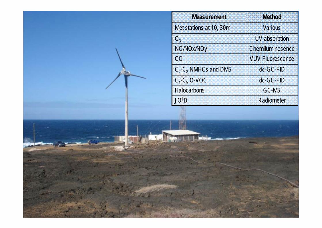
Measurement MethodMet stations at 10, 30m VariousO UV b tiO3 UV absorptionNO/NOx/NOy ChemiluminesenceCO VUV FluorescenceC2-C8 NMHCs and DMS dc-GC-FIDC1-C5 O-VOC dc-GC-FIDH l b GC MSHalocarbons GC-MSJO1D Radiometer

Dispersion footprints of air arriving at Cape Verde

1) Atlantic and African coastal,  2) Atlantic marine,  3) N th A i d Atl ti 4) N th A i d t l Af i3) North American and Atlantic 4) North American and coastal African, 5) European,  6) African,   7) European and African

NAME model.  Z. Fleming

Contribution of the main footprints to the air arriving at the stationarriving at the station

100100

80

ecto

r

Coastal African

60

of e

ach

se Polluted marine (Europe) Saharan Africa (Dust) Atlantic continental (North America)Atlantic marine

40

trib

utio

n o Atlantic marine

20

% c

on

0

1/20

07

7/20

07

1/20

08

7/20

08

1/20

09

7/20

09

1/20

10

7/20

10

1/20

11

7/20

11

01/0

1

01/0

7

01/0

1

01/0

7

01/0

1

01/0

7

01/0

1

01/0

7

01/0

1

01/0

7

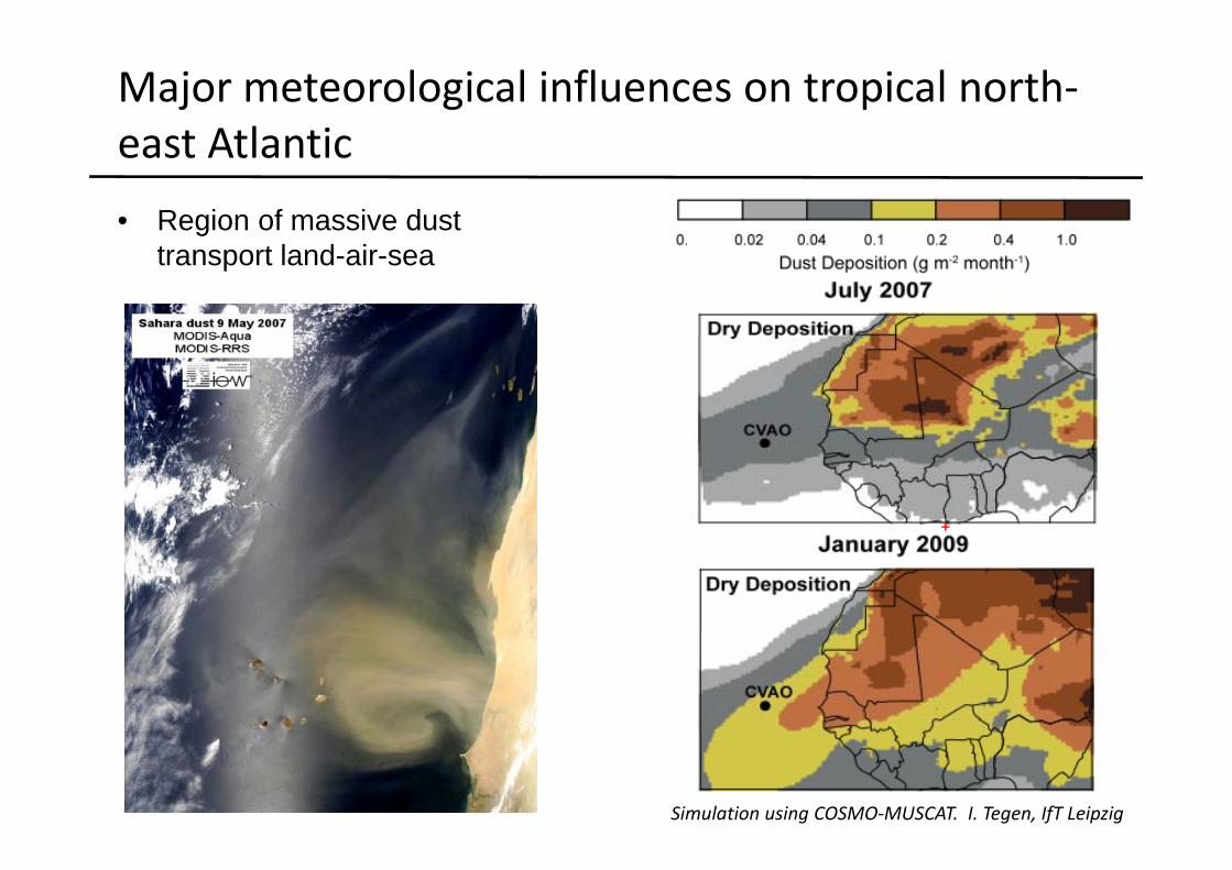
Major meteorological influences on tropical north‐east Atlantic• Region of massive dust

east Atlantic

transport land-air-sea

Simulation using COSMO‐MUSCAT.  I. Tegen, IfT Leipzig 

Dust aerosol plots from K. Muller, IfT Leipzig

Dust Marine

Dust aerosol

Fe and Al data from E. Achterberg, NOC

Suppression of atmospheric O3 by dust? 

•Marine O3/CO ratios range between 0.3–0.45•Dust O3/CO slope significantly lower (0.13)•NOy (mainly HNO3) lower in African air – despite known loss of HNO3 to dust  

Links between Saharan dust and NOy/NOx?

Redox chemistry on atmospheric dust?

Or meteorology?

Global NOx emission sourcesAfrican/dusty air – typical trajectories

Contribution of soil NOx emissions to [NOx] at Cape Verde

GEOS‐Chem output.  M. Evans

GEOS‐Chem underestimates remote MBL [NOx] and [NOy]

Red = GEOSCHEM pptBlack = meas ppt

•Model underestimates NO by factor ~ 2 and NO2 by ~ 3‐4•Unlikely to be instrument artefact (measurement uncertainty 20 % in NO at 5 pptv NO and 30% in NO2 at 10 pptv NO2)

Impact on modelled surface ozone

•Percentage increase in simulated surface O concentration when NO•Percentage increase in simulated surface O3 concentration when NOxconcentrations in the latitude range 30oS to 30oN are forced to the observational mean at Cape Verde GEOS‐Chem output.  M. Evans

Potential effect of dust on marine biological production

Effects of nutrient (N, P, Fe) additions on primary productivity (= CO2 fixation) and N2fixation in natural plankton communities of the tropical Atlantic

Circles: nutrient enrichment bioassays –stimulation of CO2 fixation, N2 fixation, Chlbiomass and bacterial productivity by dust

J. LaRoche and M. Mills

Oxygenated volatile organic compounds (OVOCs)

Atmospheric OVOCs OH loss in marine boundary layer

Methanol

Ocean: source or sink?

N

Cape Verde Atmospheric

Anthropogenic andbiomass burning sources

NOAcetoneObservatory (CVAO)Biogenicsources

CH3C(O)O2

NO2 PANHO2

organic acids

hυ, O2, OH

Primary and secondary sources

acids

HCHO, HOx, CH3O2hυ, O2, OH

AcetaldehydeSource of HOx, O3 and PAN  

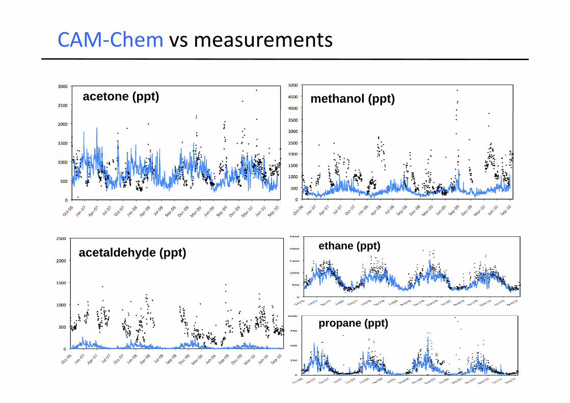
CAM‐Chem vs measurements

acetone (ppt) methanol (ppt)

ethane (ppt)acetaldehyde (ppt) ethane (ppt)

propane (ppt)

Oceans – source or sink for OVOCs? 

Model calculations indicate that the ocean is a net sink for methanol, except for over the tropical Pacific and generally a net source of acetaldehyde

•New measurements of oceanic OVOCsover Atlantic (Rachael Beale and Philover Atlantic (Rachael Beale and Phil Nightingale, PML)•April‐May 2009‐Mauritanian upwelling•October ‐ December 2009 – AMT cruise 

The AMT cruise track superimposed on the major current systems of the Atlantic Ocean between 50°N t 50°S d it AVHRR50°N to 50°S and on composite AVHRR sea surface temperature images

Modelled OVOC ocean fluxes•Sea air flux F k (C C /H) l/k 1/k + 1/Hk

308.00E‐12

•Sea‐air flux  F = kt (Cw – Ca /H)       l/kt = 1/kw +  1/Hka

25

30

6.00E‐12

8.00E 12

ms‐1)

)

20

2.00E‐12

4.00E‐12

speed ( m

km m

‐2s‐1

10

15

0.00E+00Dec Jan Mar Apr May Jun Jul Aug Sep Oct Nov Dec an

d wind 

OC flu

x (k

5

10

‐4.00E‐12

‐2.00E‐12

SST (oC) a

OVO

0‐6.00E‐12

CH3CHO CH3COCH3 CH3OH SST U 10CH3CHO CH3COCH3 CH3OH SST U 10m

Modelled (GEOS‐5) and measured wind speed

•With a squared wind dependence for sea‐air fluxes, the difference between 10 m s‐1 and 6 m s‐1 is a factor ~310 m s and 6 m s is a factor  3.

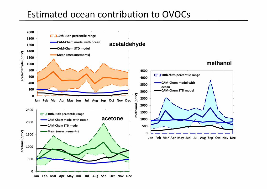
Estimated ocean contribution to OVOCs1/1/07 20/2/07 11/4/07 31/5/07 20/7/07 8/9/07 28/10/07

1400

1600

1800

2000

1400

1600

1800

2000

)

10th‐90th percentile range

CAM‐Chem model with ocean

CAM‐Chem STD modelacetaldehyde

800

1000

1200

1400

800

1000

1200

1400

ldeh

yde (pptV) Mean (measurements)

45001/1/07 20/2/07 11/4/07 31/5/07 20/7/07 8/9/07 28/10/07

4500

methanol

0

200

400

600

200

400

600

aceta

3000

3500

4000

3000

3500

4000

V)

10th‐90th percentile range

CAM‐Chem model with oceanCAM‐Chem STD model

25001/1/07 20/2/07 11/4/07 31/5/07 20/7/07 8/9/07 28/10/07

250010th‐90th percentile range

00Jan Feb Mar Apr May Jun Jul Aug Sep Oct Nov Dec

1500

2000

2500

1500

2000

2500

metha

nol (pp

tV1500

2000

1500

2000

pptV)

CAM‐Chem model with ocean

CAM‐Chem STD model

Mean (measurements)

acetone

0

500

1000

0

500

1000

Jan Feb Mar Apr May Jun Jul Aug Sep Oct Nov Decm

500

1000

500

1000

aceton

e (p Jan Feb Mar Apr May Jun Jul Aug Sep Oct Nov Dec

0

500

0

500

Jan Feb Mar Apr May Jun Jul Aug Sep Oct Nov Dec

2500 250001/01/2007 20/02/2007 11/04/2007 31/05/2007 20/07/2007 08/09/2007 28/10/2007

4500 450001/01/2007 20/02/2007 11/04/2007 31/05/2007 20/07/2007 08/09/2007 28/10/2007

10th 90th til methanol

Modelled contribution from different sources

2000 2000

10th‐90th percentile rangeMean (measurements)CAM‐Chem STD modelSTD‐NOANTHSTD‐NOBIOSTD‐NOFIRECAM Chemmodel with ocean

3000

3500

4000

) 3000

3500

400010th‐90th percentile rangeMean (measurements)CAM‐Chem STD modelSTD‐NOANTHSTD‐NOBIOSTD‐NOFIRECAM‐Chem model with ocean

acetone methanol

1000

1500

aceton

e (pptV)

1000

1500CAM‐Chem model with ocean

1500

2000

2500

methano

l (pp

tV

1500

2000

2500

CAM Chem model with ocean

0

500

0

500

0

500

1000

0

500

1000

1800

2000

1800

200001/01/2007 20/02/2007 11/04/2007 31/05/2007 20/07/2007 08/09/2007 28/10/2007

10th‐90th percentile rangeM ( )

0

Jan Feb Mar Apr May Jun Jul Aug Sep Oct Nov Dec

0 0

Jan Feb Mar Apr May Jun Jul Aug Sep Oct Nov Dec

0

1200

1400

1600

1800

e (pptV)

1200

1400

1600

1800Mean (measurements)CAM‐Chem STD modelSTD‐NOANTHSTD‐NOBIOSTD‐NOFIRECAM‐Chem model with ocean

acetaldehyde

400

600

800

1000

acetaldehyde

400

600

800

1000

0

200

Jan Feb Mar Apr May Jun Jul Aug Sep Oct Nov Dec

0

200

Observed/modelled bias vs modelled fractional contributions

y = 20.02x + 0.59

R2 = 0.39

y = 3.39x + 0.28

R2 = 0.71y = ‐3.08x + 3.44

R2 = 0.832.5

3.0

3.5

delle

d acetone

1.0

1.5

2.0

Obs

erve

d/m

od

Fractional contribution to each species from biogenic (green)

0.0

0.5

0.00 0.10 0.20 0.30 0.40 0.50 0.60 0.70 0.80 0.90 1.00

biogenic (green), anthropogenic (purple) and biomass burning (red) sources as calculated fromFractional contribution to acetone 

y = 520.33x ‐ 1.88y = 220.41x + 1.21120

sources as calculated fromCAM‐Chem.

Grey lines indicate 1:1R2 = 0.76R2 = 0.57

y = ‐289.51x + 289.87

R2 = 0.7660

80

100

d/m

odelled

Grey lines indicate 1:1 observation:modelagreement.

20

40

Obs

erve

acetaldehyde0

0.00 0.10 0.20 0.30 0.40 0.50 0.60 0.70 0.80 0.90 1.00

Fractional contribution to acetaldehyde

acetaldehyde

Correlations with anthropogenic tracer

10000

1000

ceto

ne (p

ptV)

10

100acGrey – measurementsBlack – CAM‐CHem

10 100 100010

propane ( pptV)10000

Black  CAM CHem

100

1000

de (p

ptV

)

10

100

acet

alde

hyd

10 100 10001

propane (pptV)

Biological (terrestrial) contribution

CumulativeCumulative LAI (m2 m-2)

2500 250001/01/2007 20/02/2007 11/04/2007 31/05/2007 20/07/2007 08/09/2007 28/10/2007

4500 450001/01/2007 20/02/2007 11/04/2007 31/05/2007 20/07/2007 08/09/2007 28/10/2007

10th 90th til methanol

Seasonal cycles

2000 2000

10th‐90th percentile rangeMean (measurements)CAM‐Chem STD modelSTD‐NOANTHSTD‐NOBIOSTD‐NOFIREC Ch d l i h

3000

3500

4000

) 3000

3500

400010th‐90th percentile rangeMean (measurements)CAM‐Chem STD modelSTD‐NOANTHSTD‐NOBIOSTD‐NOFIRECAM‐Chem model with ocean

acetone methanol

1000

1500

aceton

e (pptV)

1000

1500CAM‐Chem model with ocean

1500

2000

2500

methano

l (pp

tV

1500

2000

2500

CAM Chem model with ocean

0

500

0

500

0

500

1000

0

500

1000

1800

2000

1800

200001/01/2007 20/02/2007 11/04/2007 31/05/2007 20/07/2007 08/09/2007 28/10/2007

10th‐90th percentile rangeM ( )

0

Jan Feb Mar Apr May Jun Jul Aug Sep Oct Nov Dec

0 0

Jan Feb Mar Apr May Jun Jul Aug Sep Oct Nov Dec

0

1200

1400

1600

1800

e (pptV)

1200

1400

1600

1800Mean (measurements)CAM‐Chem STD modelSTD‐NOANTHSTD‐NOBIOSTD‐NOFIRECAM‐Chem model with ocean

acetaldehyde

400

600

800

1000

acetaldehyde

400

600

800

1000

0

200

Jan Feb Mar Apr May Jun Jul Aug Sep Oct Nov Dec

0

200

Conclusions

•Nitrogen oxide abundance maximises in winter in the tropical east Atlantic, showing a similar temporal variability to African dust

•How much of this is related to (i) atmospheric lifetime of NOx (ii) transport/co‐location of sources (soil) and/or (iii) chemistry occurring on dust?on dust?

•Could co‐deposition of atmospheric reactive nitrogen and dust ti l t i bi l i l d ti i th t i l Atl ti ?stimulate marine biological production in the tropical Atlantic?

•What is the impact of missing marine NOx sources on atmospheric h i ?chemistry?

•Oxygenated VOC abundance in the remote marine environment is significantly underestimated (particularly CH3CHO and CH3OH)

•Marine and biological terrestrial sources of OVOCs could explain some of this model underestimation – more work required to establish emissions  

Acknowledgements

Funding:Funding:

Technical support at CVAO:

Luis Mendes Neves Helder Lopez

Where/what form is the NOx coming from?

2 99 1 447 008.00

Observed/modelled bias vs chl‐a exposure

methanoly = 2.99x + 1.44

R2 = 0.23

y = ‐0.47x + 1.51

R2 = 0.043.004.00

5.006.007.00

served/m

odelled methanol

0.001.002.00

0.00 0.20 0.40 0.60 0.80 1.00 1.20

% of maximum back‐trajectory weighted Chl‐A

Obs

y = ‐57.62x + 58.72

R2 = 0.23

y = ‐2.20x + 5.5260

80

100

/modelled acetaldehyde

y

R2 = 0.08

0

20

40

Observed/

standard modelocean model

0.00 0.20 0.40 0.60 0.80 1.00 1.20

% of maximum back‐trajectory weighted Chl‐A

y = ‐1.21x + 1.943 00

3.50y    1.21x + 1.94

R2 = 0.17

y = ‐1.32x + 2.65

R2 = 0.14

1.00

1.50

2.00

2.50

3.00

bserved/modelled acetone

0.00

0.50

0.00 0.20 0.40 0.60 0.80 1.00 1.20

% of maximum back trajectory weighted Chl‐A

Ob

Gross primary productivity (GPP) in the Sahel