METEOROLOGICAL USES OF' THE STEREOGRAPHIC HORIZON MAP PROJECTION

br William E . Shenk Goddard Space Flight Center

'1 Hugh Powell r Computer Applications, Inc.

and

Vincent Salomonson and William R. Bandeen Goddard Space Flight Center

N A T I O N A L AERONAUTICS A N D SPACE A D M I N I S T R A T I O N W A S H I N G T O N , D. C. FEBRUARY 1971

/c 1 !! i

- %I1

https://ntrs.nasa.gov/search.jsp?R=19710007087 2018-06-15T10:09:58+00:00Z

1. Report No. XASA TN D-7009 I Government Accession No.

4. T i t l e and Subtitle

Meteorological Uses of the Stereographic Horizon Map Projection

7. Author(s) W.E. Shenk, H. Powell, V. Salomonson, & W.R. Bandeen

9. Performing Organization Name and Address

Goddard Space Flight Center Greenbelt, Maryland 2077 1

2. Sponsoring Agency Name and Address

National Aeronautics and Space Administration Washington, D. C. 20546

5. supplementary Notes

6. Abstract

TECH LIBRARY KAFB,NM

013370b

3. Recipient's Cotolog No.

5. Report Dote ~

December 1970 6. Performing Organization Code

8. Performing Organization Report No.

0. Work Uni t No. G-1012

1. Contract or Grant No.

3. Type of Report and Period Covered

Technical Note

4.3ponsoring Agency Code

The stereographic horizon map projection is a generalized form of the polar stereographic projection that permits placement of the map center at any point on the earth. With this projection, it is possible to view translating meteorological systems in one perspective regardless of system location. An algorithm was developed for con­verting a polar stereographic projection to a stereographic horizon projection. A dis­tortion analysis showed that linear distortions relative to the map center are less than 10% within 35" of great circle arc from the center. Two types of meteorological sys­tems were examined with meteorological satellite infrared radiation data placed in the new map projection to illustrate its use. The cloud pattern evolution (as seen through an infrared atmospheric window) associated with a rapidly developing extratropical storm was used to depict how the stereographic horizon map projection quantitatively reveals the major centers of cloud development, movement, and dissipation relative to the cyclone center. With the stereographic horizon projection, the classical dynamic

i features of the jet stream appeared to be present in the appropriate quadrants of a composite of Nimbus 3 infrared (6.4 to 6.9 pm) radiation data surrounding 13jet stream speed maxima.

L 7. Key Words Suggested by Author 18. Distribution Statement

Unclassified-Unlimited

?.Security Classif . (of th is report) 20. Security Classif . (of this page)

Unclassified Unclassified 19 $3.00

For sale by the National Technical Information Service, Springfield, Virginia 22151

/’

CONTENTS

Page

INTRODUCTION . . . . . . . . . . . . . . . . . . . . . . . . . . . . . . . . . . . . . . . . . . . . . . . . . . . . . . . . . . . . . . 1

MAP GEOMETRY . . . . . . . . . . . . . . . . . . . . . . . . . . . . . . . . . . . . . . . . . . . . . . . . . . . . . . . . . . . . . . 1 Conversion from True to Pseudo Coordinates . . . . . . . . . . . . . . . . . . . . . . . . . . . . . . . . . . . . . 2 Grid Print Map Coordinates . . . . . . . . . . . . . . . . . . . . . . . . . . . . . . . . . . . . . . . . . . . . . . . . . . . 3 Map Distortion . . . . . . . . . . . . . . . . . . . . . . . . . . . . . . . . . . . . . . . . . . . . . . . . . . . . . . . . . . . . . 4

EXAMPLES OF METEOROLOGICAL USES OF THE PROJECTION . . . . . . . . . . . . . . . . . . . . . 8 TrackingofaCyclone . . . . . . . . . . . . . . . . . . . . . . . . . . . . . . . . . . . . . . . . . . . . . . . . . . . . . . . 8 Jet Stream Analysis . . . . . . . . . . . . . . . . . . . . . . . . . . . . . . . . . . . . . . . . . . . . . . . . . . . . . . . . . 13

CONCLUDING REMARKS . . . . . . . . . . . . . . . . . . . . . . . . . . . . . . . . . . . . . . . . . . . . . . . . . . . . . . . 18

References . . . . . . . . . . . . . . . . . . . . . . . . . . . . . . . . . . . . . . . . . . . . . . . . . . . . . . . . . . . . . . . . . . . . 19

c \

L

... 111

I -

&\

x.

METEOROLOGICAL USES OF THE STEREOGRAPHIC HORIZON MAP PROJECTION

by William E. Shenk

Goddard Space Flight Center Hugh Powell

Computer Applications, In e. Vincent Salomonson and William R. Bandeen

Goddard Space Flight Center

INTRODUCTION

The analysis of meteorological data is usually performed on some standard map projection, such as the Mercator or polar stereographic projections. Cyclones and other translating weather features are displayed and tracked on the map base. The amount of distortion caused by the geometry of the.pro­jection vanes as the feature moves, depending on the type of projection and the change in latitude of the moving feature. It is often very advantageous to view translating weather phenomena in a Lagran­gian sense, that is, to have the map projection translate with the system. For example, it would be use­ful to have the pole of a polar stereographic projection located at the center of a tropical cyclone and have the map projection translate with the cyclone. Thus, the map distortions remain the same rela­tive to the center regardless of the location of the cyclone.

One map projection that satisfies this objective is called the stereographic horizon projection (Deetz and Adams, 1944). It is essentially a polar stereographic projection with the property that the pole can be placed at any point on the globe. The movable pole can be placed at a common position relative to a sequence of views of a given system, and hence the weather feature can be anaiyzed with the same perspective throughout its lifetime. Further, similar weather features can be examined with a common reference point over a lengthy period of record leading to a climatological analysis of these features.

MAP GEOMETRY

The stereographic horizon projection is defined as the projection of the earth’s surface onto a plane tangent to the earth’s surface at the map center, the vertex of the projection being the point on the earth diametrically opposite the map center.

Figure 1 shows a point P on the earth that is located on the map by extending the chord to P’.Point C on the earth is coincident with C‘ (the center of the map). Any point on earth can be

1

PSEUDO EQUATOR

Figure 1-A side view of the stereographic horizon map projection showing the projection of a point P on a globe onto the projection at point P'.

specified as the map center, including the North and South Poles, and any type of data for any known location can be placed on the stereographic horizon map base.

A projection extensively used for the display of meteorological information is the polar stereo-graphic projection. The geometry described be­low transfers the data from a polar stereographic projection (with the projection plane tangent to the earth at the pole) to the stereographic horizon projection.

Conversion from True Coordinates to Pseudo Coordinates

Figure 2 shows the geometrical relationship between points C and P. The true latitude h d

longitude (GP,Ap) of point P were converted to pseudo latitude and pseudo longitude (P,, up),with the map center as the pseudo pole designated by latitude and longitude (G,, A,).

From Figure 2, cos (90" - PP ) = r . ro, where r and ro are vectors extending from the center of the

earth to P(GP,Ap) and C($,, A,) respectively. The expressions for r and ro are given by

r = i c o s ~ p c o s A p + j c o s ~ p s i n AP + k s i n G p , (1)

ro = i cos 4, cos A, +j cos 4, sin A, + k sin G, , (2)

where i, j, and k are unit vectors. Therefore,

cos (90" - P p ) = sin PP = cos Ij, cos A, cos @P cos AP + cos G, sin A, cos GP sin Ap + sin G, sin GP . (3)

Computations were performed only for sin p p >0. Thus, no computations were made for P in the opposite hemisphere.

The pseudo longitude of P,up,is computed from the law of sines and law of cosines for a spheri­cal triangle:

cos GP sin (A, - Ap) sin u

P =

cos Pp > (4)

sin @ p - sin @, sin PP COSU

P = cos @, cos Pp (5)

Computation of both sin up and cos up is required in order to locate up in the proper quadrant.

2

N Grid Print Map Coordinates

C = CENTER OF MAP, THE PSEUDO POLE

N = TRUE POLE

0 = CENTER OF EARTH P = POINT TO BE LOCATED

*p, Ap = TRUE LATITUDE, LONGITUDE OF P eC,Ac = TRUE LATITUDE, LONGITUDE OF C

B p , ap = PSEUDO LATITUDE, LONGITUDE OF P

3r COP = 9OO-B d: NCP = a

Figure 2-Geometrical relationshipsbetween the true pole, N, the pseudo pole of the stere­ographic horizon projection, C, and an arbi­trary point, P, on the surface of a globe.

A convenient method of displaying meteorological in­formation is to use a computer-generated grid print map. These maps are created by placing the data at equally spaced increments on the map. Thus, in the case of the stereographic horizon projection relative to the center of the map, the x and y coordinates of each data location must be known. With the knowledge of P p , the map scale factor, and the diameter of the earth, we can now compute the distance d on the stere­ographic horizon map between points P' and C (Figure 3). The relationships for D and d are given by

diameter of the earth -D = map scale factor - scaled diameter of the earth ,

d = D tan "i] = D tan y .

In the computation of the grid print map coordinates x and y from the center of the map, three different cases are considered:

(1) Map centered at North Pole. (2) Map centered at South Pole. (3) Map centered at any other point (stereographic

horizon map).

Prior to the calculationof x andy in all three cases, the data within the stereographichorizon map can be rotated about the center by specifying an azimuth, z, to be added to the west pseudo longitude, up. Figure 4 diagrams the three cases with a rotational azimuth added. All longitudes in the following dis­cussion, whether pseudo or true, are west longitudes.

Case 1. North Pole Map

In both polar cases the pseudo latitude and pseudo longitude < p p ,uc) are equal to the true values ?* (A ,@ ). Westerly longitudes increase clockwise from the positive x abscissa which is the starting point

. pbyp hstorical convention. Therefore, the expressions for the x and y coordinates of P' are

x = d cos (up+ z ) and

y = - d sin (ap+ z ) .

Case 2. South Pole Map

Westerly longitudes increase counterclockwise from the negative x abscissa. As a result, the x and y coordinates for P' are

3

- -

P-l P' c'

D = DIAMETER OF THE EARTH MAP SCALE

d = DISTANCE ON MAP BETWEEN CENTER AND POINT P'

C = PSEUDO POLE (THE MAP CENTER)

8 p = PSEUDO LATITUDE OF POINT P

P = POlFiT TO BE LOCATED

90"-8pY = 2

Figure 3-An edgewise view of the stereographic horizon projection illustrating the distance d between the map projection center, C', and the projected point, P'.

Case 3. Stereographic Horizon Map

The longitude was arbitrarily selected to in­crease clockwise from the positive y ordinate. Thus, the x and y coordinates for P' are

x = d sin (up+ z ) (1 1)and

y = d cos (up+ z ) . (12)

Map Distortion

A comparison of portions of the map surface with the corresponding global surface was made as a function of latitude from the map center. First, the length of a segment of a meridian on the stereographic horizon map was compared with the length of the corresponding arc on the globe. Fig­ure 5 shows a stereographic horizon map which is centered at the pole C. Points A and B lie on the same meridian at latitudes @2 and and are pro­

jected-onto the map at A' and B'. The length of the arc mon the globe is to be compared with the line A'B' on the map. Since the length of the entke meridian equals the circumference of the globe, 2rR, the length of the arc AB (hereafter called Mg)would be

Mg= 27rR (s). -

The distance A'B' on the map is obtained by subtracting B T from A T . It can be seen that 6AOC = 90" - @2, and from plane geometry it follows that 4ADC = ?h&AOC. Therefore,

A'C= 2R tan too;@j= 2R tan (45" - Yz@~),

and, similarly, -B'C= 2R tan (45O ­

-Thus, A'B' on the map (hereafter called M,) would be

M , = A'C -B'C= 2R [tan (45" - - tan (45" -%@,)I (16).

4

NORTH POLE MAP SOUTH POLE MAP STEREOGRAPHIC HORIZON MAP c = +go c = -90 +go> c > -90

P' - POINT TO BE LOCATED ON THE STEREOGRAPHIC HORIZON MAP

C - CENTER OF THE MAP d - DISTANCE FROM CENTER TO POINT P', A FUNCTION OF THE LATITUDE

(OR PSEUDO LATITUDE) OF P Z - AZIMUTH, SUPPLIED BY THE USER TO "ROTATE" THE MAP IF DESIRED a - LONGITUDEJPSEUDO LONGITUDE FOR THE STEREOGRAPHIC HORIZON MAP)

OF POINT P x, y - COORDINATES OF THE MAP RELATIVE TO THE CENTER

Figure 4-The geometry of the calculation of x and y grid print map coordinates corresponding to an arbitrary point P' on the three possible types of stereographic projections with a rotational azimuth, Z, added.

Table 1 gives the lengths of M , and Mg for a 5" arc - r$2 = 5") centered at different lati­tudes, the radius of the globe being set equal to 1.O. Notice that M , is exaggerated as the arc is moved away from the pole, whereas Mg remains constant. The degree of exaggeration is expressed as M , /Mg.

The length of a parallel on the globe with its projected length on a stereographic horizon map was compared. Figure 6 depicts the parallel on the globe at latitude r$, having a radius rg, and the projection of this parallel onto the map, with a

R = RADIUS OF THE EARTH radius rm. The length of the parallel Pg on the Figure 5-Distortion of an arc length, Mg,between points globe is given by A and 6 along a meridian on a globe of unit radius when it is projected onto the stereographic horizon map (M,,,). Pg = 2rrg = 2n(R cos 4) . (17)

5

I

1- STEREOGRAPHIC HORIZON /

I II I I

Figure 6-The calculation of map distortion around a lati­tude circle as a function of pseudo latitude by the com­parison of the total length of the parallel on a globe of unit radius (PJ with the total length of the parallel on the stereographic horizon map (P,,,).

From (14), the length of the parallel (P,) on the map would be

P, = 2nr,

= 27r[2R tan (45" - %@)I

= 47rR tan (45" - %G) . (18)

?able 1-Comparison of the length of a 5" arc long a meridian on a globe of unit radius with he length (M,) of the arc when projected on the tereographic horizon map. The length (Mg)of a i o arc on a globe of unit radius is 0.08727.

Latitude of Arc Length Exaggeration Arc Center on the Map . Factor

(deg.1 (M,) (M,/Mg)

5 0.16068 1.84068 10 .14878 1.70492 15 .1387 1 1.58949 20 .13010 1.49087 25 .12273 1.40635 30 .1 1639 1.33375 35 .11095 1.27135 40 .lo627 1.21776 45 .lo226 1.17185 50 .09885 1.13272 55 .09596 1.09964 60 .09355 1.07200 65 .09157 1.04933 70 .09000 1.03127 75 .08879 1.01750 80 .08795 1.00782 85 .08745 1.00206 90 .08728 1.00016

~

Table 2 gives the values of P, and P, for the latitude of the centers of the same 5" arcs used in the computation of M , and M,. The exaggeration P,/P, is approximately equal to the exaggeration M,/Mg along the meridian for all latitudes.

A comparison was also made between the area of a zone on the globe and the corresponding area on the stereographic horizon map. Figure 7 shows the projection of a shaded zone onto the map. The area of the shaded zone on the globe is given by

A, = 27rRh ,

where

h = h, - h, = R(sin 4, - sin GA)

Therefore,

A, = 27rR2(sin GB - sin GA) ,

6

I

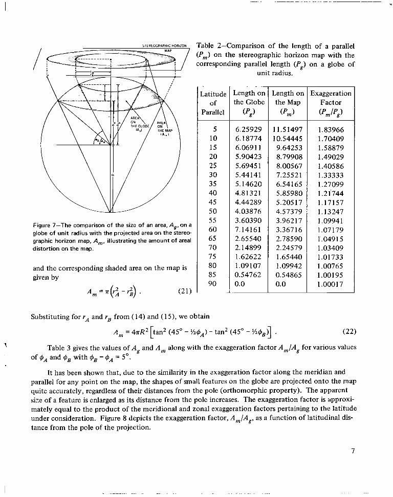
Table 2-Comparison of the length of a parallel (P,) on the stereographic horizon map with the corresponding parallel length (P,) on a globe of

Figure 7-The comparison of the size of an area, A,, on a globe of unit radius with the projected area on the stereo-graphic horizon map, A,,,, illustrating the amount of areal distortion on the map.

and the corresponding shaded area on the map is given by

A m = n r 2 - 'B) ' (21)( A 2

unit radius. ~~

Latitude Length on Length on Exaggeration of the Globe the Map Factor

Parallel (P,) (P,) (P,/P,)

5 6.25929 11.51497 1.83966 10 6.18774 10.54445 1.70409 15 6.0691 1 9.64253 1.58879 20 5.90423 8.79908 1.49029 25 5.6945 1 8.00567 1.40586 30 5.44141 7.25521 1.33333 35 5.14620 6.54165 1.27099 40 4.8 132 1 5.85980 1.2 1'744 45 4.44289 5.205 17 1.17157 50 4.03876 4.57379 1.13247 55 3.60390 3.962 17 1.09941 60 7.14161 3.367 16 1.07179 65 2.65540 2.78590 KO49 15 70 2.14899 2.24579 1.03409 75 1.62622 1.65440 1.01733 80 1.09107 1.09942 1.00765 85 0.54762 0.54865 1.00 195 90 0.0 0.0 1.00017

Substituting for rA and rB from (14) and (1 5), we obtain -

.Am = 4nR2 ban2 (45" - - tan2 (45" - %@B)l 7 Table 3 gives the values of A, and A , along with the exaggeration factor Am/Agfor various values

of and @B with $B - @A = 5".

It has been shown that, due to the similarity in the zxaggeration factor along the meridian and parallel for any point on the map, the shapes of small features on the globe are projected onto the map quite accurately, regardless of their distances from the pole (orthomorphic property). The apparent size of a feature is enlarged as its distance from the pole increases. The exaggeration factor is approxi­mately equal to the product of the meridional and zonal exaggeration factors pertaining to the latitude under consideration. Figure 8 depicts the exaggeration factor, A,/A,, as a function of latitudinal dis­tance from the pole of the projection.

7

.. ......-....... .... .. . .. . . . . . .. . .. . . .-.

Table 3-Comparison of area (A,) on the stereo- EXAMPLES OF METEOROLOGICAL graphic horizon map with area (A,) on a globe of USES OF THE PROJECTION

unit radius.

Latitudes Area on Area on Exaggeration - the Globe the Map Factor @A @B (A,) (A,) -

0 5 0.54762 2,01436 3.67933 5 10 .54345 1.70368 3.13494

10 15 .535 15 1.44887 2.70743 15 20 .52277 1.23779 2.36776 20 25 .50641 1.06100 2.095 13 25 30 .48620 0.9 1138 1.87448 30 35 .46230 0.78343 1.69465 35 40 .43487 0.67289 1.54734 40 45 .40413 0.57642 1.42632 45 50 .37032 0.49 133 1.32677 50 55 .33369 0.4 1546 1.24506 55 60 .2945 1 0.34704 1.17836 60 65 .25310 0.28461 1.12446 65 70 .20976 0.22692 1.08177 70 75 .16483 0.17290 1.04895 75 80 .11864 0.12162 1.02512 30 85 .07 155 0.07223 1.00956 35 90 .02391 0.02396 1.00189 -

90" 80' 70" 60" 50' 40" 30" 20" IO' 0'

PSEUDO LATITUDE FROM MAP CENTER

Figure 8-The areal exaggeration factor, A,/Ag, as a func­tion of pseudo latitudefrom the center of the stereographic horizon map.

Tracking of a Cyclone

The great advantage of viewing a weather system in the same perspective as it translates is illustrated by viewing an extratropical cyclone in the stereographic horizon and Mercator map pro­jections on two consecutive days. A western Pa­cific cyclone center moved from 40"N, 149"E at 1400 GMT on November 10, 1966, to 49"N, 157"E twenty-four hours later. Figures 9 and 10 show the National Meteorological Center (NMC) surface charts for 1200 GMT on November 10 and 11, 1966, respectively. The cyclone deep­ened and intensified rapidly during the 24-hour interval, the central pressure falling from 1006 mb at the beginning of the period to 987 mb at the end.

In this example, the data to be shown in the stereographic horizon and Mercator map projec­tions are the emitted terrestrial radiation sensed in the 3.5 to 4.1 pm atmospheric "window" by the high resolution infrared radiometer (HRIR) on board the Nimbus 2 meteorological satellite. Since in this wavelength region thermal emission and reflected solar radiation contribute about equally to the observed radiance during the day­time, reasonable meteorological interpretations of terrestrial radiation patterns can be made only at night. Under clear sky conditions, the radiances (which are converted to equivalent blackbody temperatures) are used to determine surface tem­peratures. Cloud heights can be inferred from the equivalent blackbody temperatures when the clouds are opaque and completely fill the field of view of the radiometer. The interpretation of equivalent blackbody temperatures below 240 K is difficult due to substantial noise in the instru­ment observations and the method of data proc­essing. A complete error analysis of the Nimbus 2 HRIR data is given by Williamson (1 969).

T

8

45'N

40%

35%

3Q0N

Figure 9-NMC surface chart for 1200 GMT, November 10, 1966.

SOON

50°N

45ON

45'N

40°N

4 0 ° N

35' N 35ON

A

30°N 3 0 ° N

Figure 10-NMC surface chart for 1200 GMT, November 11, 1966.

9

I

c

Detailed information concerning the Nimbus 2 satellite and the HRIR experiment is available in the "Nimbus I1 Users' Guide.""

One form of displaying the rectified infrared data is to use the grid print map for various map pro­jections and scales. The algorithms described in the previous section allow the data to be assembled on the stereographic horizon projection in grid print form. More description of the grid print map display can be found in the "Nimbus I1 Users' Guide" and in other publications, such as Warnecke et al. (1968).

The Mercator and stereographic horizon projections, Figures 11 and 12, respectively, show the radiation pattern composite (orbits 2386 and 2387) associated with the extratropical storm for the first day. The. frontal positions, adjusted for the time of the satellite pass, were taken from analyses prepared by NMC. Low equivalent blackbody temperatures, clearly depicted near the center of each map, indicate the main cloud mass associated with the cyclone. The shape of the solid cloud deck suggests a storm in the early stage of rapid development (Brodrick, 1969). An indication of dry air intruding into the cloud mass is shown by the notch in the isolines of equivalent blackbody tempera­ture just west of the position of the low center on the surface chart. The position of the stationary front between 25" and 30"N is corroborated by the relatively low equivalent blackbody temperature (cloud) band stretching east-northeast to west-southwest at a substantial distance to the southwest of the cyclone center.

The map scale for each projection is 1:5,000,000. Whereas the scale factor is true at the pole (center of the map) for the stereographic horizon projection, it is true at 22.5" north or south of the equator for the Mercator projections. The cyclone appears smaller in the stereographic horizon projec­tion because of the properties of the Mercator projection with the cyclone center at 40"N. If the cy­clone center were at 22.5"N, then the system would look similar in both projections. Not only is the apparent map factor different for the two views of the system, but the change in map distortion across the cyclone's cloud mass is greater for the Mercator projection. This results in the impression that a large portion of the cloud deck is north of the cyclone center. A glance at the stereographic horizon map shows that the proportion of the cloud mass north of the center to the total cloud mass is less than that suggested by the Mercator map.

Figures 13 and 14 view the cyclone in the two projections 24 hours later, after the storm has moved some 9" of latitude farther north. The cloud mass associated with the storm has expanded con­siderably, especially to the southeast of the storm center, and has assumed the shape of an inverted fishhook. This shape is characteristic of a cyclone that is nearing maximum intensity (Brodrick, 1969).

Since the storm has moved poleward, the differences between the Mercator and stereographic L horizon projections are more striking than on the f i s t day. With increasing latitude, the cloud shield size becomes proportionally greater on the Mercator map base. The cloud mass north of the storm center now has become greatly distorted relative to the cloud mass of the entire system.

Table 4 was prepared to illustrate quantitatively the scale difference between the two projections and the distortion change with increasing latitude on a Mercator map. The entries in the table are the number of grid intersections on the grid print maps within the 255 K isotherm, which essentially

*Nimbus Project, NASA Goddard Space Flight Center, Greenbelt, Maryland, 229 pp., 1966.

10

Table 4-The number of grid intersections (orbits 2399-2400) within the 255-K isotherm bounding the major cloud mass associated with the low pressure center shown in Figures 13 and 14.

Latitude Mercator

Map Projection ("1

Stereographic Horizon Map Projection

(N,1

Comparison R ("INs)

55" to 60"N 206 75 2.82 50" to 55"N 316 139 2.27 45" to 50"N 138 68 2.03 40" to 45"N 90 59 1.53 35" to 40"N 64 48 1.33

bounded the cloud mass associated with the cyclone in Figures 13 and 14. The ratio of the number of grid intersections in the Mercator projection to the number of grid intersections in the stereographic horizon projection within each 5" latitude band increased with increasing latitude. Between 55' and 60"N, the ratio was 2.82, and between 35" and 40'N the ratio was still substantially greater than unity.

From a meteorological point of view, the most striking chart of this series is an equivalent black­body temperature difference chart (Figure 15), where the temperatures displayed in Figure 12 (orbits 2386-87) were subtracted from the temperatures depicted in Figure 14 (orbits 2399-2400) in the stereographic horizon projection. It should be emphasized that this difference map was easily calcu­lated with the stereographic horizon projection, whereas it would have been far more difficult to cre­ate by other means. Figure 15 essentially reveals the changes in the cloud deck relative to the cyclone center in the 24-hr period. The greatest change occurred to the southeast of the storm center, where the cloud mass developed substantially, as noted by the -60 K differences and the large area covered by differences of more than -50 K. Large positive equivalent blackbody temperature differences (20 to 50 K) indicate the position of the cloud band associated with the subtropical stationary front south­west of the cyclone center on the first day and the subsequent movement of the band from that posi­tion relative to the storm center. From the conventional data, it is most likely that the polar cold front further north on the first day merged with the subtropical stationary front, and this combined front swept southward. The smaller negative equivalent blackbody temperature differences south of the axis of the positive equivalent blackbody temperature differences noted above indicate that the cloud band weakened.

t Near the low center is another area of large positive equivalent blackbody temperature differ­ences, which are associated with the dry air that encircles the center. The smaller positive differences north-northwest of the center are the result of higher equivalent blackbody temperatures on the sec­ond day, a common occurrence as cyclones reach peak intensity. East of this combined area of posi­tive equivalent blackbody temperatures lies a large area of negative equivalent blackbody temperatures, which reflects the expansion of the cloud shield east of the storm center.

In general, the equivalent blackbody temperatures were lower on the second day (Figure 14). As a result, most of the differences shown in Figure 15 are negative. Since the cyclone was located 9' of

11

Figure 11-Infrared (3.5 to 4.1 pm) radiation equivalent blackbody temperature (K) pattern associatedwith the ex­tratropical storm centered at 40°N, 149'E shown in a Mercator map projection. Stippled areas indicate where the equivalent blackbody temperatures are less than 250 K.

latitude farther north on the second day, the ocean temperature background beneath the clouds was lower than on the first day. Although with HRIR data there is no way to test independently for the presence or absence of clouds, the large area of negative values (1 to 5 K) some 20" of latitude south of the storm center probably is representative of this effect. This amount of ocean temperature change is consistent with the climatological ocean temperatures for November presented by LaViolette and Seim ( 1 969).

12

5O”N

M0N

4 f N

1 49N

4O0N

40°N

3?N

35ON

3cfh

MON

25%

25 N

Figure 12-The same equivalent blackbody temperature (K) pattern shown in Figure 11 in the stereographic horizon map projection. The concentric circles are pseudo co-latitude distances from the map center. Stippled areas indicate where the equivalent blackbody temperatures are less than 250 K.

Jet Stream Analysis

The stereographic horizon projection can be used to ascertain if consistent patterns relative to certain features of jet stream flow are discernible in the equivalent blackbody temperature patterns observed by satellite radiometers. As an illustration of this capability, a composite of equivalent

13

'E

&PN

w o

4Oo

M O N

T

the

14

Figure 14-The same equivalent blackbody temperature ( K ) pattern shown in Figure 13 in the stereographic horizon map projection. The concentric circles are pseudo co-latitude distances from the map center.

blackbody temperatures in the Nimbus 2 medium resolution infrared interferometer (MRIR) 6.4 to 6.9 pm, 10 to 11 pm, and 5 to 30 pm spectral response regions were assembled on a 1 :10 million ster­eographic horizon map for appropriate situations occurring during the period May 20 to July 28, 1966. The composites were formed from 23 orbits and provided data coverage for 13 individual jet stream cases occurring over or near the continental United States. The locations of the jet maxima ranged between 29" and 47"N and 82" and 115"W.

15

Figure 15-Equivalent blackbody temperature (K) difference chart where the temperatures displayed in Figure 12 (orbits 2386-87) are subtracted from the temperatures shown in Figure 14 (orbits 2399-2400). The concentric circles are pseudo co-latitude distances from the map center.

Y

In each of the jet stream cases, the stereographic horizon grid was centered at a location corre-Isponding to that of a concomitant wind speed maximum. The location of the jet stream and the asso­

ciated wind speed maximum were determined from 200-mb7300-mb7maximum wind speed, and wind shear analyses prepared by NMC. Because the Nimbus orbits do not cross the United States at the standard 0000 and 1200 GMT map times associated with the synoptic analyses just mentioned, it was necessary to locate the wind speed maximum at two successive map times surrounding the MRIR ob­servation time. Once this was accomplished the position of the speed maximum was adjusted to corre­spond to the time of satellite passage. The difficulty associated with establishing the positions of a wind speed maximum at two successive times from only the NMC analyses resulted in only 13 cases

16

Figure 16-Composited equivalent blackbody temperatures measured in the 6.4 to 6.9 pm spectral region and associated with 13 jet stream cases where the stereographic horizon map center is located at the wind speed maximum. In each individual je t stream case, a constant azimuth was added to each data point so that all data would be assembled relative to the x-axis of the stereographic horizon projection.

17

i

1

being selected from the May 20 to July 28 period. Once the speed maximum was located, a constant azimuth, z, was determined for each individualjet stream case that was added to the pseudo longitude ap of each point in the stereographichorizon map. The magnitudes of the azimuth were decided by de­termining the amount that the data should be rotated in order to bring all data parallel to the direction of flow through the wind speed maximum such that these data were parallel to the x-axis of the stere­ographic horizon projection (see Figure 4). The magnitude of z ranged from 92" to -44". The pur­pose of this procedure was to form a composite of the observed equivalent blackbody temperatures relative to the jet stream flow passing through the wind speed maximum.

Figure 16 shows the results arising from the compositing procedure in the case of the 6.4 to 6.9 pm MRIR water vapor channel. The response in this channel is related to the amount of moisture in the upper troposphere; i.e., the magnitude of the equivalent blackbody temperatures varies inversely with the amount of moisture. As can be seen in Figure 16, a band of warmer temperatures extends from a position to the rear and left of the speed maximum into the lower right quadrant. There is also a band of lower equivalent blackbody temperatures to the right of the jet, primarily in the lower left quadrant, and another area of lower temperatures in the upper right quadrant. The relative locations of these warmer and colder equivalent blackbody temperature areas, which are most likely associated with convergence and divergence, respectively, are in agreement with results predicted by an advective approximation of the vorticity equation (Reiter, 1963). The pronounced band of colder temperatures to the right of the jet is associated with higher amounts of moisture and clouds of the cirrus type. In general, the results described here are in agreement with studies reported by Johnson and Shen (1967) and Beran et al. (1968) involving radiometric measurements and with studies such as those by Reiter and Whitney (1969) and Whitney et al. (1966) utilizing satellite camera observations.

The reasonable nature of the results described above and the contribution that the horizontal stereographic projection makes in facilitating the consistent assembling of the radiometric satellite data indicate that this technique can be very useful for further studies relating quasi-horizontal fields of emitted radiation to the dynamic characteristics of the jet stream.

CONCLUDING REMARKS

The horizontal stereographic map projection has considerable value for meteorological analysis. Normalization of the viewing perspective and different orientations of translating meteorological sys­tems can be achieved. The projection permits the compositing of data such that the climatologies of translating systems can be examined more efficiently. Further, statistical analysis can be performed more easily where measurements for weather systems are consistently located in the same perspective. Undoubtedly, other meteorological applications for the use of the stereographic horizon projection will emerge as the Lagrangian property of viewing meteorological systems is exploited.

Goddard Space Flight Center National Aeronautics and Space Administration

Greenbelt, Maryland, July 8 , 1970 160-44-51-01-51

r

i

I

18

~~ . .. ... ... .. . . . ..-_ ~ ..__

REFERENCES

Beran, D. W., Merritt, E. S., and Chang, D. T., “Interpretation of Baroclinic Systems and Wind Fields as Observed by Nimbus I1 MRIR,” Allied Research Report 96-43-F, Allied Research Associates, Concord, Massachusetts, 135 pp., 1968.

I Brodrick, H. J., Jr., “Some Aspects of the Vorticity Structure Associated with Extratropical Cloud

Systems,” Environmental Science Services Administration Technical Memorandum NESCTM 15, U.S. Dept. of Commerce, Washington, D. C., 8 pp., 1969.

Deetz, C. H., and Adams, 0. S., Elements of Map Projection 5th Edition, Revised, U. S. Govt. Printing Office, Washington, D.C., 226 pp., 1944.

Johnson, D. R., and Shen, W. C., “Profiles of Infrared Irradiance and Cooling Through a Jet Stream,” Studies of Large Scale Atmospheric Energetics annual report prepared under Environmental Science Services Administration Grant WBG-52 by the Department of Meteorology, Univ. of Wisc., Madison, pp. 7 1-95, 1967.

LaViolette, P. E., and Seim, S. E., “Monthly Charts of Mean, Minimum, and Maximum Sea Surface Temperature of the North Pacific Ocean,” Naval Oceanographic Office, SP-123, Washington, D.C., 57 pp., 1969.

Reiter, E. R., Jet Stream Meteorology University of Chicago Press, Chicago, Illinois, 5 15 pp., 1963.

Reiter, E. R., and Whitney, L. F., “Interaction Between Subtropical and Polar Front Jet Stream,” Monthly Weather Review 97, pp. 432-438, 1969.

Warnecke, G., Allison, L. J., Kreins, E. R., and McMillin, L. M., “A Satellite View of Typhoon Mane 1966 Development,” NASA Technical Note D-5 142, National Aeronautics and Space Administra­tion, Washington, D.C., 47 pp., 1968.

Whitney, L. F., Jr., Timchalk, A., and Gray, T. I., Jr., “On Locating Jet Streams from TIROS Photo­1

graphs,” Monthly Weather Review 94, pp. 127-138, 1966.

I Williamson, E. J., “The Accuracy of the High Resolution Infrared Radiometer on Nimbus II,” NASA Technical Note D-555 1,National Aeronautics and Space Administration, Washington, D.C., 14 pp., 1969.

I NASA-Langley, 1971 - 13 19

NATIONAL AND SPACE ADMINISTRATAERONAUTICS ION

WASHINGTON, D. C. 20546

OFFICIAL BUSINESS

0 3 U 001 38 51 3 C S A I R F O R C E WEAPGNS K I R T L A N D A F B , NEki

A T 1 E, LOU B O W P A R ,

FIRST CLASS MAIL

POSTAGE A N D FEES PAID NATIONAL AERONAUTICS A N D

SPACE ADMINISTRATION

7 1 0 2 8 00903 L A B O R A T C R Y /kLOL/ M E X I C O 87117

CHIEF,TECH. L I B K A R Y

If Undeliverable (Section 158POSTMASTER: Postal Manual) Do Nor Return ,

"The aeronaiitical and space activities of the United States shall be conducted so as t o contribute . . . t o the expansion of human knowl­edge of phenomena in the atmosphere and space. The Adniinistrntion shall provide for the widest practicable and appropriate dissemination of information concerning its activities and the 7eSdtS thereof."

-NATIONALAERONAUTICSA N D SPACE ACT OF 1958

NASA SCIENTIFIC A N D TECHNICAL PUBLICATIONS

TECHNICAL REPORTS: Scientific and technical information considered important, complete, and a lasting contribution to existing knowledge.

TECHNICAL NOTES: Information less broad in scope but nevertheless of importance as a contribution to existing knowledge.

TECHNICAL MEMORANDUMS: Information receiving limited distribution because of preliminary data, security classifica­tion, or other reasons.

CONTRACTOR REPORTS: Scientific and technical information generated under a NASA contract or grant and considered an important contribution to existing knowledge.

TECHNICAL TRANSLATIONS: Information published in a foreign language considered to merit NASA distribution in English.

SPECIAL PUBLICATIONS: Information derived from or of value to NASA activities. Publications include conference proceedings, monographs, data compilations, handbooks, sourcebooks, and special bibliographies.

TECHNOLOGY UTILIZATION PUBLICATIONS: Information on technology used by NASA that may be of particular interest in commercial and other non-aerospace applications. Publications include Tech Briefs, Technology Utilization Reports and Technology Surveys.

Details on the availability of these publications may be obtained from:

SCIENTIFIC AND TECHNICAL INFORMATION OFFICE

NATIONAL AERONAUTICS AND SPACE ADMINISTRATION Washington, D.C. PO546

1