method of least work - asad iqbalengrasad.weebly.com/uploads/1/4/2/1/14213514/lecture_4.pdf ·...
TRANSCRIPT
Method of Least Work
Theory of Structures‐II M Shahid Mehmood
Department of Civil Engineering
Swedish College of Engineering & Technology, Wah Cantt

Method of Least Work / Castigliano’s Second Theorem
• Force Method
• Compatibility equations are established by using theCastigliano’s second theorem, instead of by deflection
i i i h d f i d f isuperposition as in method of consistent deformations.
• Let us consider a statically indeterminate beam withi ldi t bj t d t t l l diunyielding supports subjected to an external loading w.
w
CBA
2
Method of Least Work / Castigliano’s Second Theorem
C
w
BA
By
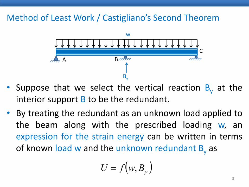
• Suppose that we select the vertical reaction By at theinterior support B to be the redundant.
• By treating the redundant as an unknown load applied tothe beam along with the prescribed loading w, an
i f h i b i iexpression for the strain energy can be written in termsof known load w and the unknown redundant By as
3
( )yBwfU ,=
Method of Least Work / Castigliano’s Second Theorem
• Above equation indicates symbolically that the strainenergy for the beam is expressed as a function of theknown external load w and the unknown redundant By.
Castigliano’s second theorem
“The partial derivative of the strain energy with respectto a force equals the deflection of the point of theapplication of the force along its line of action”application of the force along its line of action .
4
Method of Least Work / Castigliano’s Second Theorem
• Since the deflection at the point of application of theredundant By is zero, by applying the Castigliano’s secondtheorem, we can write
∂U 0=∂∂
yBU
• It should be realize that this equation represents thecompatibility equation in the direction of redundant By,and it can be solved for the redundantand it can be solved for the redundant.
• This equation states that the first partial derivative of thestrain energy with respect to the redundant must bestrain energy with respect to the redundant must beequal to zero.
5
Method of Least Work / Castigliano’s Second Theorem
• This implies that for the value of the redundant thatsatisfies the equations of equilibrium and compatibility,the strain energy of the structure is a minimum ormaximummaximum.
Si f li l l ti th i i l f• Since for a linearly elastic, there is no maximum value ofstrain energy, because it can be increased indefinitely byincreasing the value of the redundant we conclude thatincreasing the value of the redundant, we conclude thatfor the true value of the redundant the strain energymust be a minimum.
6
Method of Least Work / Castigliano’s Second Theorem
• This conclusion is known as Principle of Least Work.
“The magnitudes of the redundants of a staticallyindeterminate structure must be such that the strainenergy stored in the structure is a minimum (i.e., thei t l k d i th l t) ”internal work done is the least).”
If i i d i h h d h• If a structure is indeterminate to the nth degree, the nredundants are selected, and the strain energy for thestructure is expressed in terms of the known externalstructure is expressed in terms of the known externalloading and the n unknown redundants as
7

Method of Least Work / Castigliano’s Second Theorem
• If a structure is indeterminate to the nth degree, the nredundants are selected, and the strain energy for thestructure is expressed in terms of the known externalloading and the n unknown redundants asloading and the n unknown redundants as
( )nRRRRwfU ,....,,,, 321=
in which w represents all the known loads and R1, R2,…,R d t th d d tRn denote the n redundants.
8
Method of Least Work / Castigliano’s Second Theorem
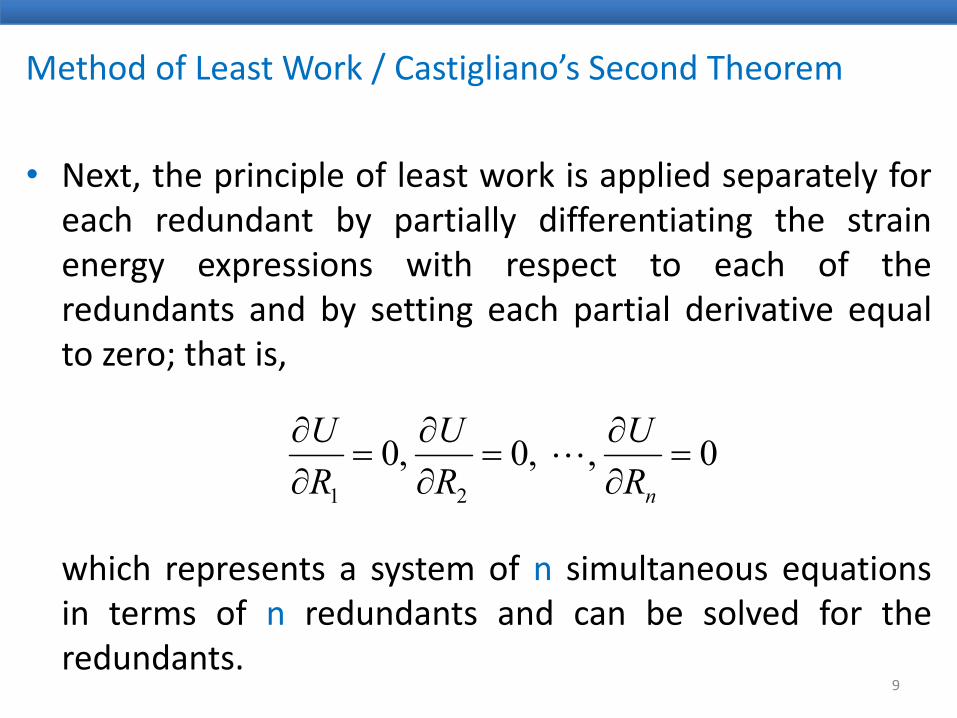
• Next, the principle of least work is applied separately foreach redundant by partially differentiating the strainenergy expressions with respect to each of theredundants and by setting each partial derivative equalredundants and by setting each partial derivative equalto zero; that is,
0 , ,0 ,021
=∂∂
=∂∂
=∂∂
nRU
RU
RU
L
which represents a system of n simultaneous equationsin terms of n redundants and can be solved for thein terms of n redundants and can be solved for theredundants.
9
Method of Least Work / Castigliano’s Second Theorem
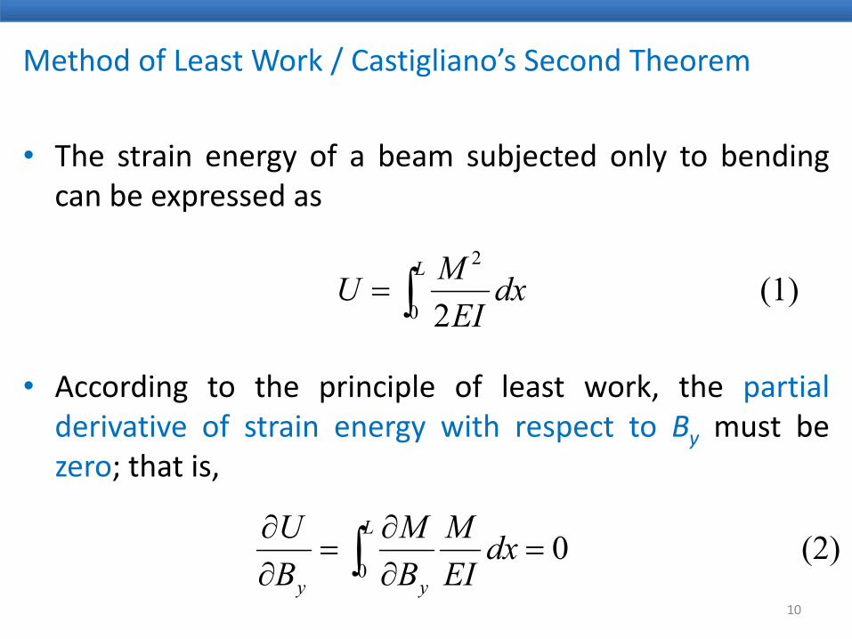
• The strain energy of a beam subjected only to bendingcan be expressed as
2ML
∫ (1) 20
dxEI
MUL
∫=
• According to the principle of least work, the partialderivative of strain energy with respect to By must be
h izero; that is,
(2)0dxMMU L
∫ =∂
=∂
10
(2) 00
dxEIBB yy
∫ =∂
=∂

Example 1
Determine the reactions for the beam shown in Fig., bythe method of least work. EI is constant.
1.6 k/ft
A B
30 ft
11

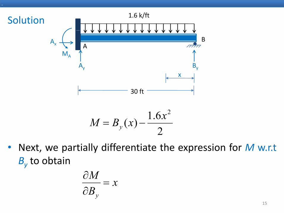
Solution
1.6 k/ft
ABAx
MA
30 ft
ByAy
MA
• The beam is supported by four reactions, so its degree ofpp y , gindeterminacy is equal to 1.
• The vertical reaction By, at the roller support B, isyselected as the redundant.
12

Solution
-
1.6 k/ft
ABAx
f
ByAy
MA
• We will evaluate the magnitude of the redundant by
30 ft
minimizing the strain energy of the beam with respect toBy.
• The strain energy of a beam subjected only to bendingcan be expressed as
2ML
∫13
(1) 20
dxEI
MUL
∫=

Solution
-
2ML
∫ (1) 20
dxEI
MU ∫=
• According to the principle of least work, the partialderivative of strain energy with respect to By must be
h izero; that is,
(2)0dxMMU L
∫ =∂
=∂ (2) 0
0dx
EIBB yy∫ =∂
=∂
• Using the x coordinate shown in Fig, we write theequation for bending moment, M, in terms of By, as
14
Solution
-
1.6 k/ft
ABAx
MA
30 ft
ByAy
x
30 ft
6.1)(2xxBM
• Next, we partially differentiate the expression for M w.r.t
2)(xBM y −=
, p y pBy to obtain
xM=
∂
15
xBy
=∂
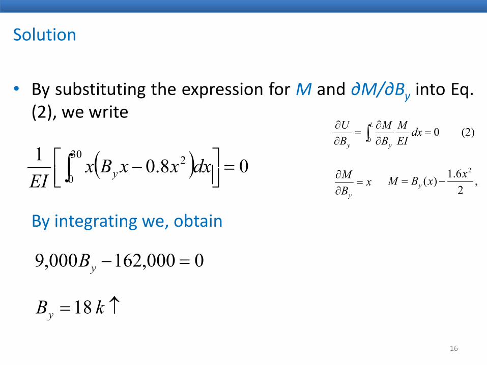
Solution
• By substituting the expression for M and ∂M/∂By into Eq.(2), we write
( )1 30 2 ∫(2) 0
0 dx
EIM
BM
BU L
yy∫ =∂∂
=∂∂
,26.1)(
2xxBM y −=xBM
y
=∂∂( ) 08.01 30
0
2 =
−∫ dxxxBx
EI y
By integrating we, obtain
00001620009 =B 0000,162000,9 =−yB
18 ↑= kB
16
18 ↑kBy
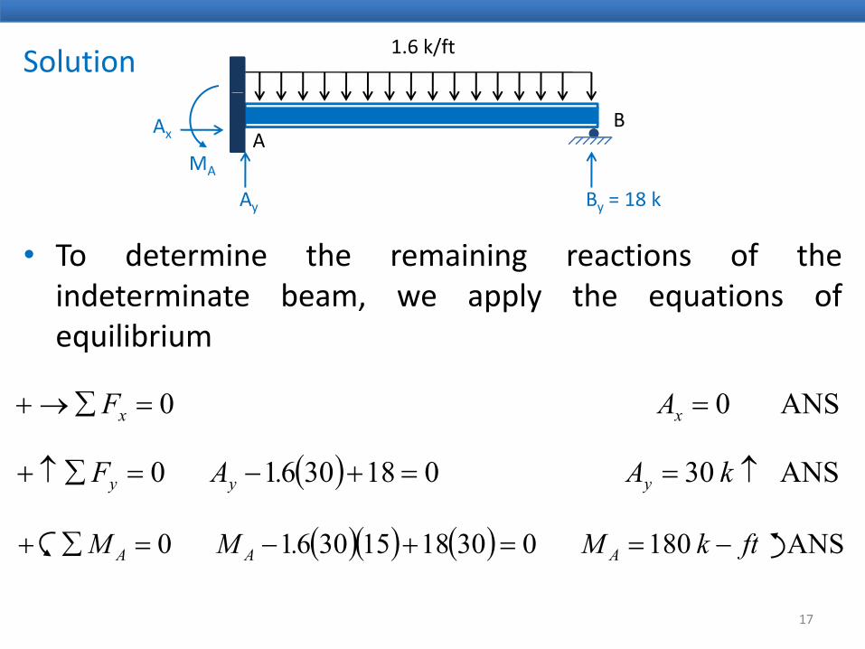
Solution 1.6 k/ft
ABAx
MA
• To determine the remaining reactions of the
By = 18 kAy
indeterminate beam, we apply the equations ofequilibrium
ANS 0 0 ==∑→+ xx AF
( ) ANS3001830610 ↑∑↑ kAAF ( ) ANS 30 01830610 ↑==+−=∑↑+ k A . AF yyy
( )( ) ( ) ANS 180030181530610 ftk M. MM AAA −==+−=∑+
17
( )( ) ( ) fAAA
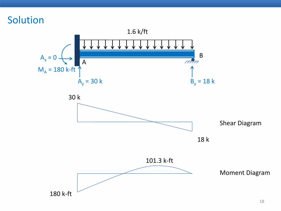
Solution1 6 k/ft
AB
1.6 k/ft
Ax = 0A
By = 18 kAy = 30 k
x
MA = 180 k‐ft
30 k
hShear Diagram
18 k
101.3 k‐ft
Moment Diagram
18
180 k‐ft
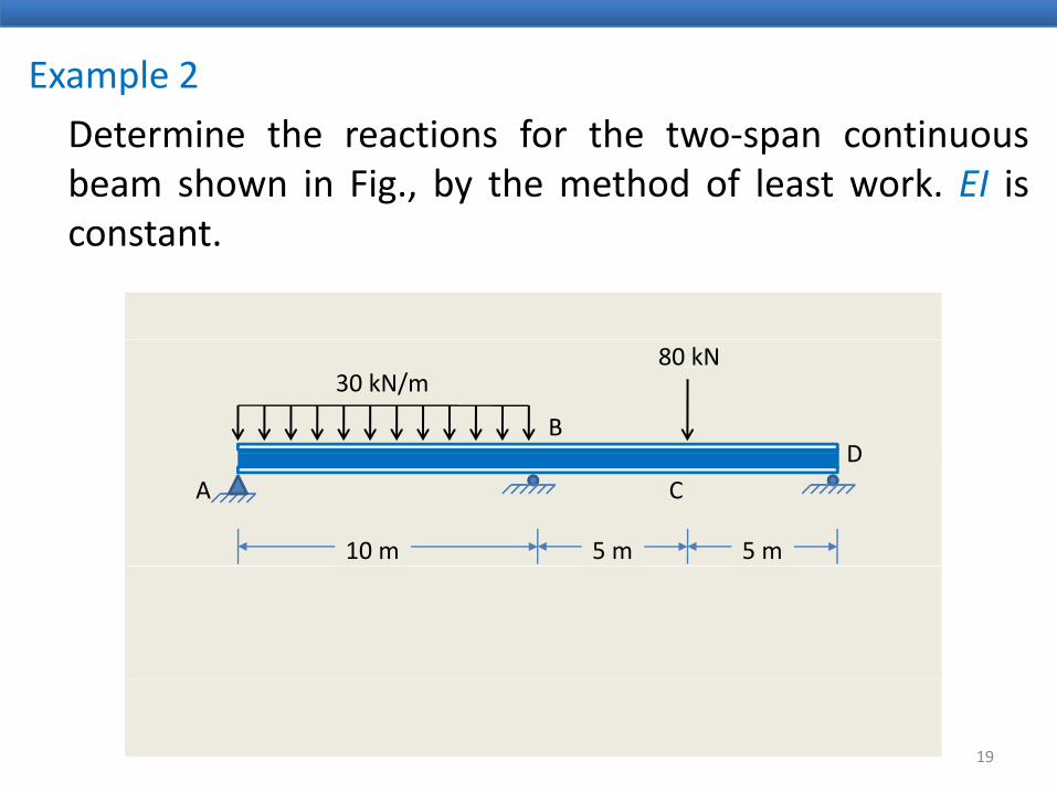
Example 2
Determine the reactions for the two‐span continuousbeam shown in Fig., by the method of least work. EI isconstantconstant.
D
30 kN/m80 kN
BD
10 m
CA
5 m 5 m
19
Solution80 kN
D
30 kN/m80 kN
BAx
CAx
Ay By Dy
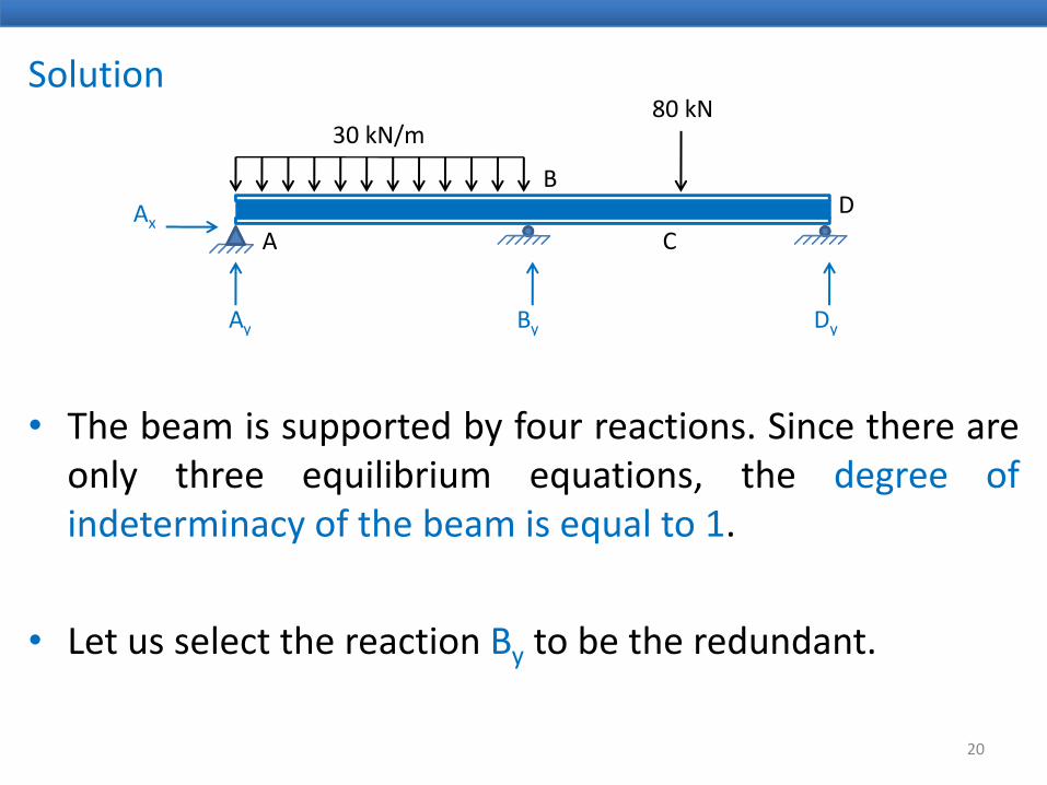
• The beam is supported by four reactions. Since there areonly three equilibrium equations, the degree ofindeterminacy of the beam is equal to 1.
• Let us select the reaction By to be the redundant.
20
Solution80 kN
D
30 kN/m80 kN
BAx
CAx
Ay By Dy
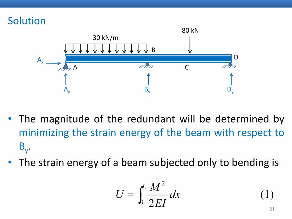
• The magnitude of the redundant will be determined byminimizing the strain energy of the beam with respect toBy.
• The strain energy of a beam subjected only to bending is
2ML
∫21
(1) 20
dxEI
MUL
∫=
Solution30 kN/m
80 kN
D
30 kN/m
C
B
AAx
Ay By Dy
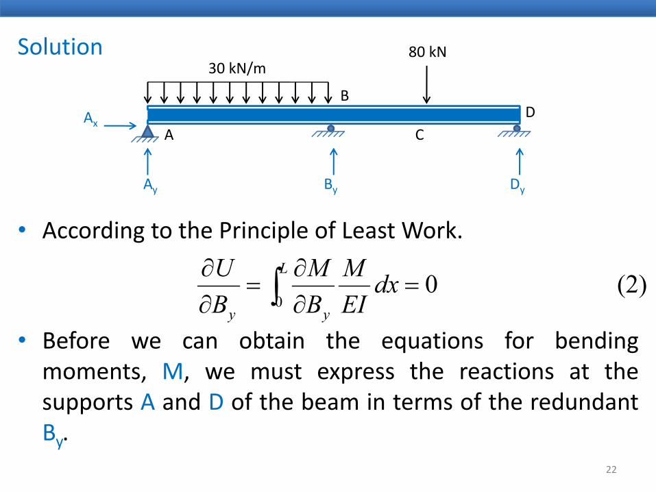
• According to the Principle of Least Work.
(2)0dxMMU L
∫∂∂
• Before we can obtain the equations for bending
(2) 00
dxEIBB yy
∫ =∂
=∂
q gmoments, M, we must express the reactions at thesupports A and D of the beam in terms of the redundantBy.
22
Solution30 kN/m
80 kN
D
30 kN/m
C
B
AAx = 0
Ay = 245 ‐ 0.5By By Dy = 135 ‐ 0.5By
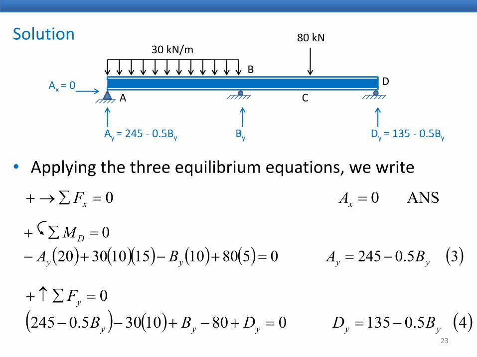
• Applying the three equilibrium equations, we write
ANS 0 0 ==∑→+ xx AF∑ xx
( ) ( )( ) ( ) ( ) ( )350245058010151030200 D
BABA M
++=∑+
( ) ( )( ) ( ) ( ) ( )3 5.0245 05801015103020 yyyy BA BA −==+−+−
0y F =∑↑+
23
( ) ( ) ( )4 5.0135 08010305.0245 yyyyy
y
BD DBB −==+−+−−
Solution30 kN/m
80 kN
D
30 kN/m
C
B
AAx = 0
Ay = 245 ‐ 0.5By By Dy = 135 ‐ 0.5By
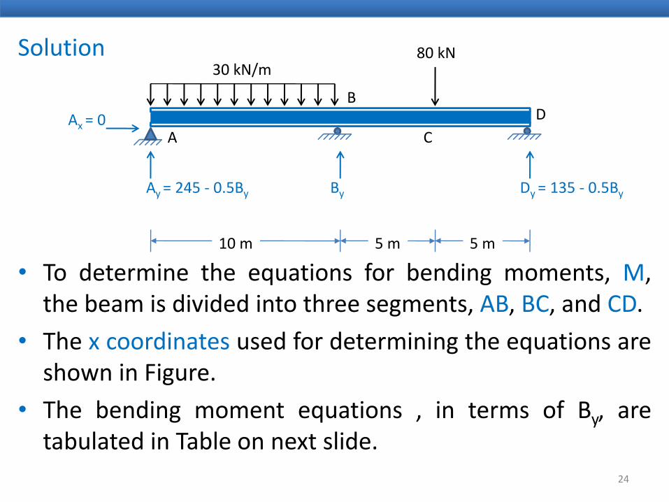
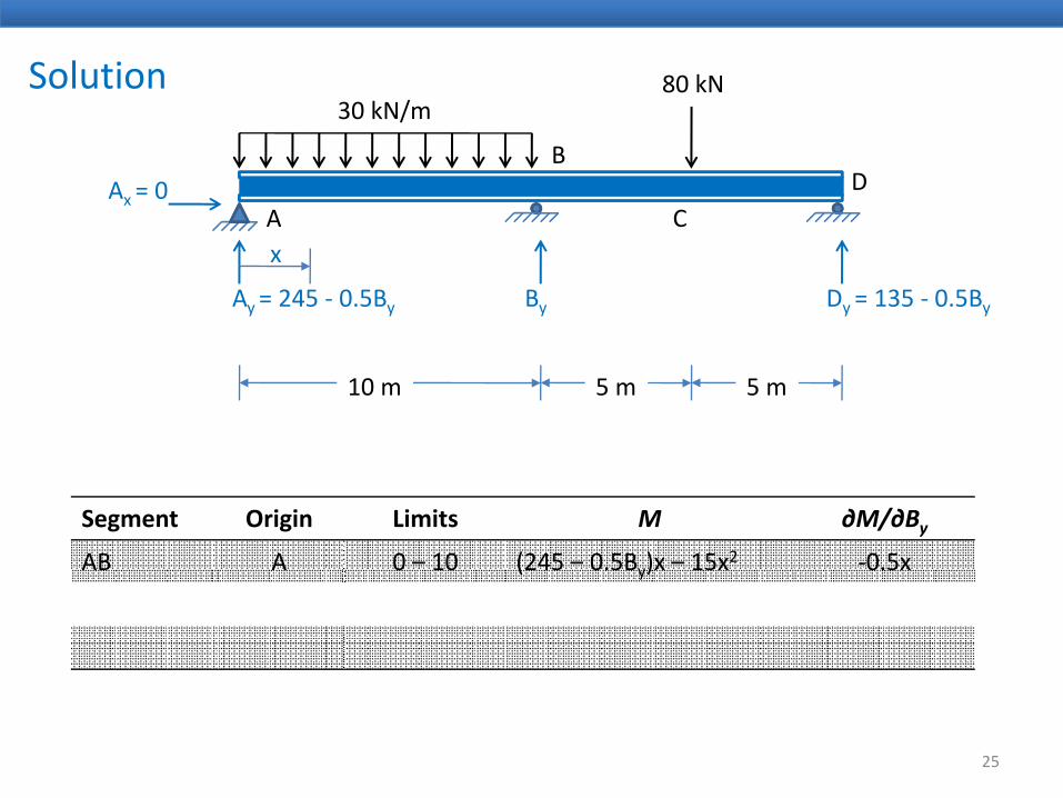
• To determine the equations for bending moments, M,10 m 5 m 5 m
the beam is divided into three segments, AB, BC, and CD.
• The x coordinates used for determining the equations areshown in Figure.
• The bending moment equations , in terms of By, aretabulated in Table on next slide.
24
Solution30 kN/m
80 kN
D
30 kN/m
C
B
AAx = 0
Ay = 245 ‐ 0.5By By Dy = 135 ‐ 0.5By
x
10 m 5 m 5 m
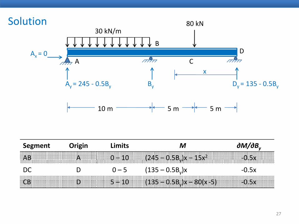
Segment Origin Limits M ∂M/∂ByAB A 0 – 10 (245 – 0.5By)x – 15x2 ‐0.5xAB A 0 10 (245 0.5By)x 15x 0.5x
25

Solution30 kN/m
80 kN
D
30 kN/m
C
B
AAx = 0
Ay = 245 ‐ 0.5By By Dy = 135 ‐ 0.5By
x
10 m 5 m 5 m
Segment Origin Limits M ∂M/∂ByAB A 0 – 10 (245 – 0.5By)x – 15x2 ‐0.5xAB A 0 10 (245 0.5By)x 15x 0.5x
DC D 0 – 5 (135 – 0.5By)x ‐0.5x
26
Solution30 kN/m
80 kN
D
30 kN/m
C
B
AAx = 0
Ay = 245 ‐ 0.5By By Dy = 135 ‐ 0.5By
x
10 m 5 m 5 m
Segment Origin Limits M ∂M/∂ByAB A 0 – 10 (245 – 0.5By)x – 15x2 ‐0.5xAB A 0 10 (245 0.5By)x 15x 0.5x
DC D 0 – 5 (135 – 0.5By)x ‐0.5x
CB D 5 – 10 (135 – 0.5By)x – 80(x ‐5) ‐0.5x
27
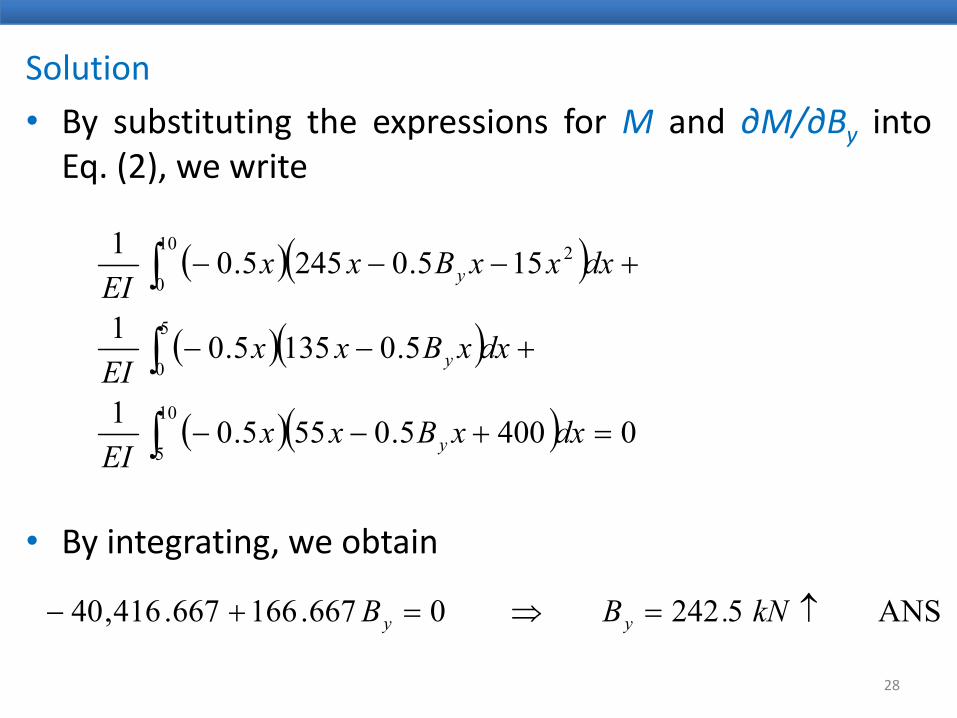
Solution
• By substituting the expressions for M and ∂M/∂By intoEq. (2), we write
( )( )155.02455.01 10
0
2 +−−−∫ dxxxBxxEI y
( )( )
( )1
5.01355.01
10
5
0+−−∫ dxxBxx
EI y
( )( ) 04005.0555.01 10
5=+−−∫ dxxBxx
EI y
• By integrating, we obtain
ANS5242066716666741640 ↑=⇒=+− kNBB
28
ANS 5242 0667.166667.416,40 ↑=⇒=+ kN.BB yy
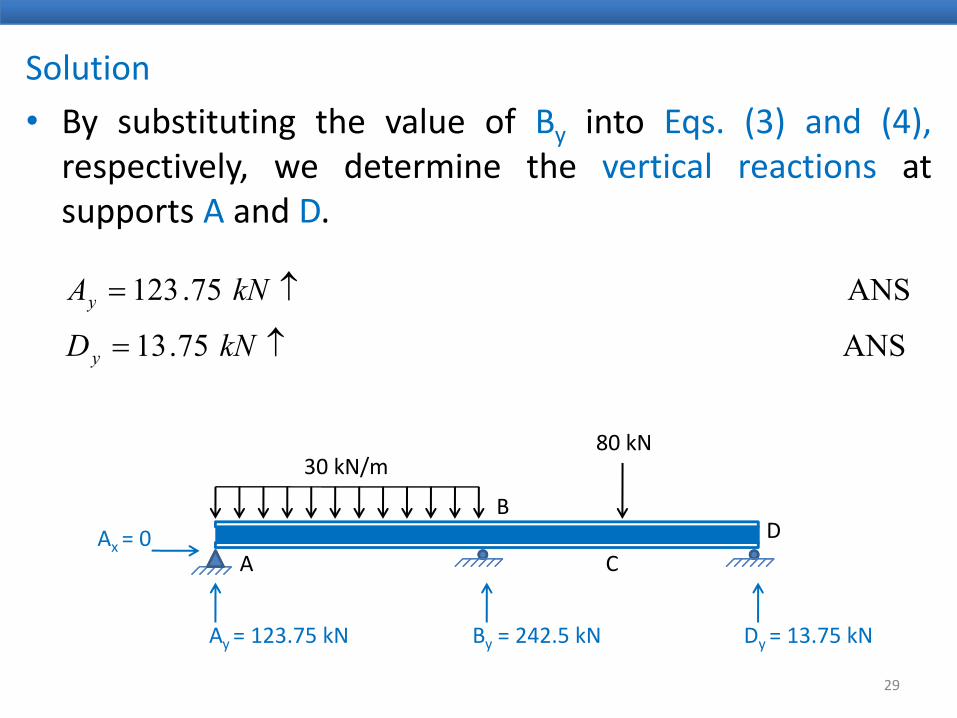
Solution
• By substituting the value of By into Eqs. (3) and (4),respectively, we determine the vertical reactions ats pports A and Dsupports A and D.
ANS 75.123 ↑= kNAy
ANS 75.13 ↑= kNDy
y
30 kN/m80 kN
BD
C
B
AAx = 0
29
Ay = 123.75 kN By = 242.5 kN Dy = 13.75 kN
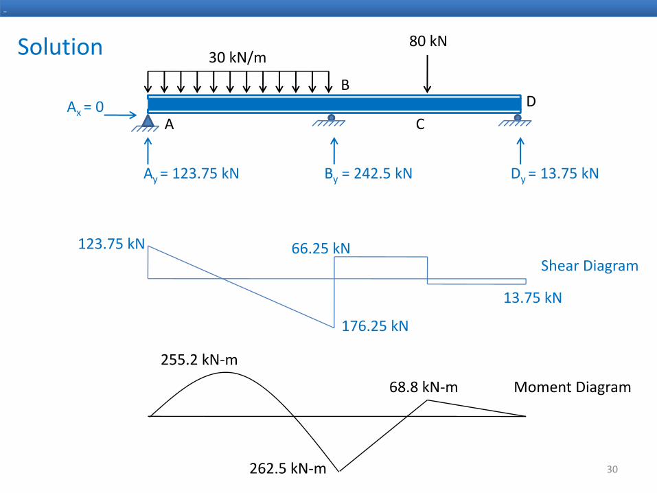
Solution
-
30 kN/m80 kN
DC
B
AAx = 0
Ay = 123.75 kN By = 242.5 kN Dy = 13.75 kN
123.75 kNShear Diagram
66.25 kN
176.25 kN
13.75 kN
Moment Diagram
255.2 kN‐m
68.8 kN‐m
30262.5 kN‐m
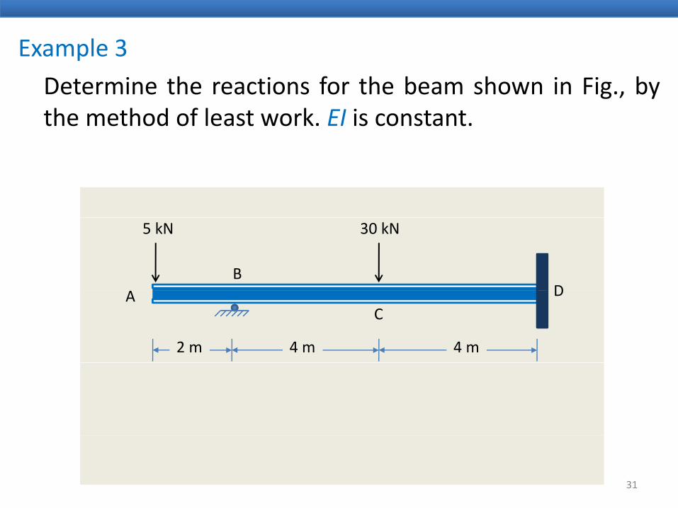
Example 3
Determine the reactions for the beam shown in Fig., bythe method of least work. EI is constant.
D
30 kN
B
5 kN
D
2 m
CA
4 m 4 m
31
Solution
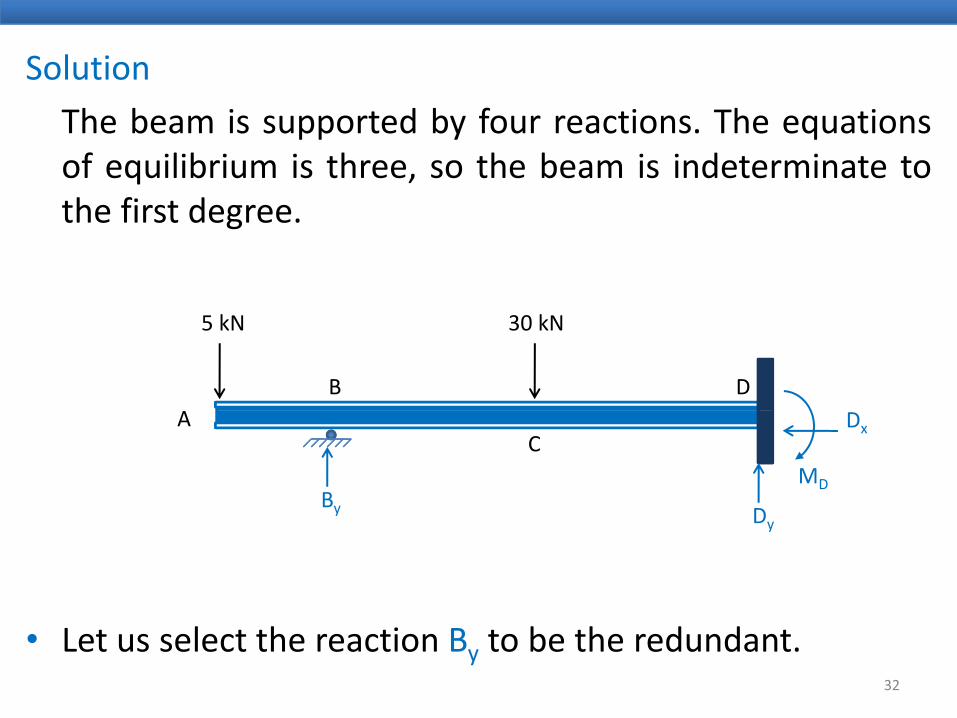
The beam is supported by four reactions. The equationsof equilibrium is three, so the beam is indeterminate tothe first degreethe first degree.
D
30 kN
B
5 kN
CA
By D
Dx
MD
y Dy
• Let us select the reaction By to be the redundant.32
Solution 30 kN5 kN
D
C
BA Dx
By Dy
MD
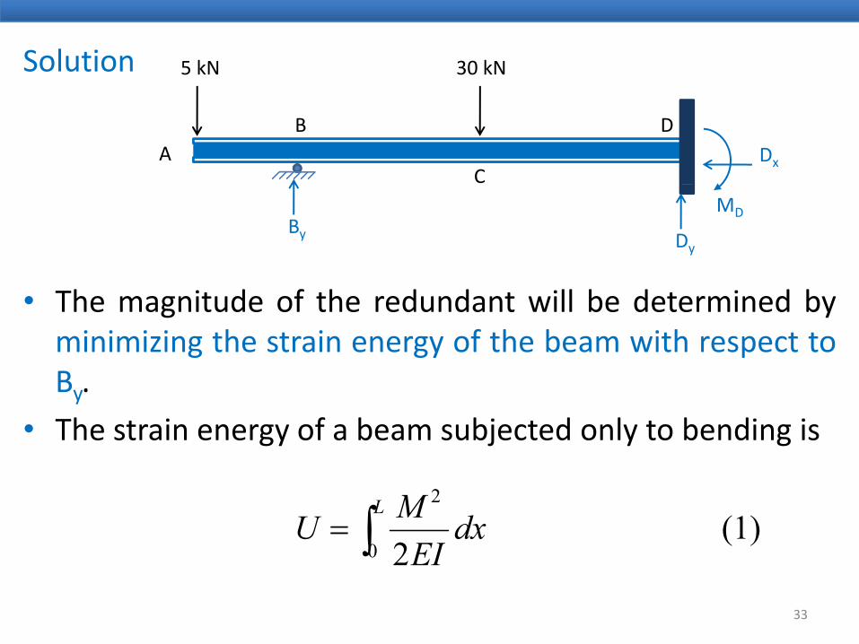
• The magnitude of the redundant will be determined byminimizing the strain energy of the beam with respect toBy.
• The strain energy of a beam subjected only to bending is
(1) 20
2
dxEI
MUL
∫=
33
20 EI∫
Solution 30 kN5 kN
D
C
BA Dx
By Dy
MD
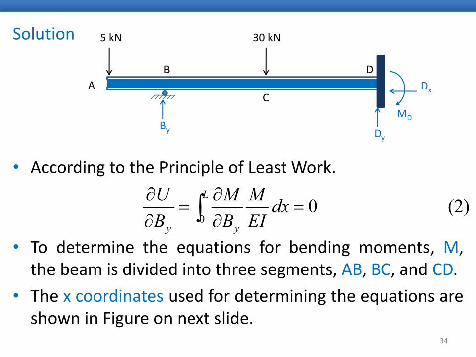
• According to the Principle of Least Work.
(2)0dxMMU L
∫∂∂
• To determine the equations for bending moments, M,
(2) 00
dxEIBB yy
∫ =∂
=∂
q g , ,the beam is divided into three segments, AB, BC, and CD.
• The x coordinates used for determining the equations areshown in Figure on next slide.
34
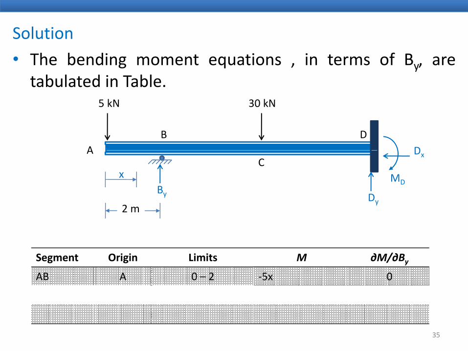
Solution
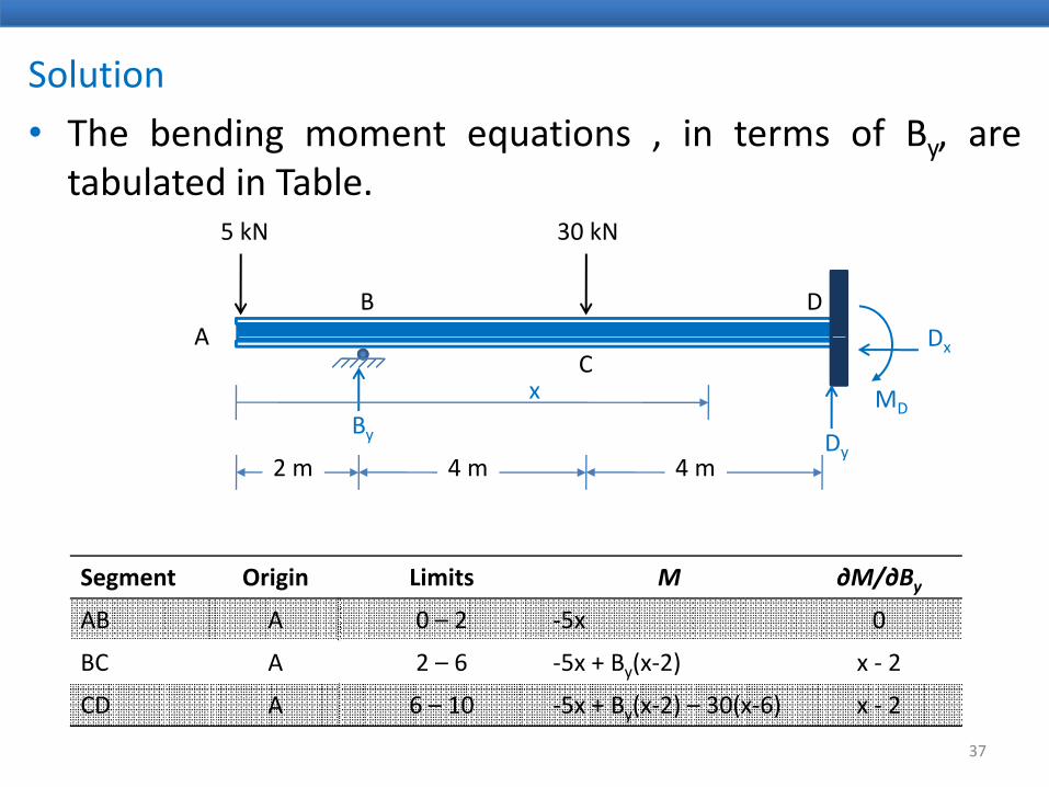
• The bending moment equations , in terms of By, aretabulated in Table.
30 kN5 kN
D
30 kN
BA
5 kN
DC
A
By Dy
Dx
MDx
Dy2 m
Segment Origin Limits M ∂M/∂ByAB A 0 – 2 ‐5x 0
35

Solution
• The bending moment equations , in terms of By, aretabulated in Table.
30 kN5 kN
D
30 kN
BA
5 kN
DC
A
By Dy
Dx
MDx
Dy2 m 4 m
Segment Origin Limits M ∂M/∂ByAB A 0 – 2 ‐5x 0
BC A 2 – 6 ‐5x + By(x‐2) x ‐ 2
36
y( )
Solution
• The bending moment equations , in terms of By, aretabulated in Table.
30 kN5 kN
D
30 kN
BA
5 kN
DC
A
By Dy
Dx
MDx
Dy2 m 4 m 4 m
Segment Origin Limits M ∂M/∂ByAB A 0 – 2 ‐5x 0
BC A 2 – 6 ‐5x + By(x‐2) x ‐ 2
37
y( )
CD A 6 – 10 ‐5x + By(x‐2) – 30(x‐6) x ‐ 2

Solution
• By substituting the expressions for M and ∂M/∂By intoEq. (2), we write
(2) 00
dxEIM
BM
BU L
yy∫ =∂∂
=∂∂
( )( ) ( )( )( )1
2251051 6
2
2
0+−−+−+− ∫∫ dxxxBx
EIdxx
EI y
( ) ( )( )( ) 02630251 10
6=−−−−+−∫ dxxxxBx
EI y
• By integrating, we obtain
ANS25160661703272773 ↑=⇒=+− kNBB
38
ANS 25.16 066.170327.2773 ↑=⇒=+ kNBB yy
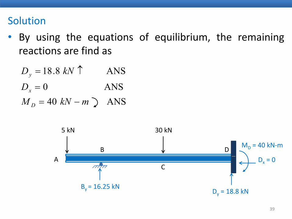
Solution
• By using the equations of equilibrium, the remainingreactions are find as
ANS 0
ANS 8.18
D kND
x
y
=
↑=
ANS 40 m kNM D −=
D
30 kN
B
5 kN
MD = 40 kN‐m
CA
B = 16 25 kN
Dx = 0
39
By = 16.25 kNDy = 18.8 kN
SolutionD
30 kN
B
5 kN
MD = 40 kN‐mD
C
BA Dx = 0
D
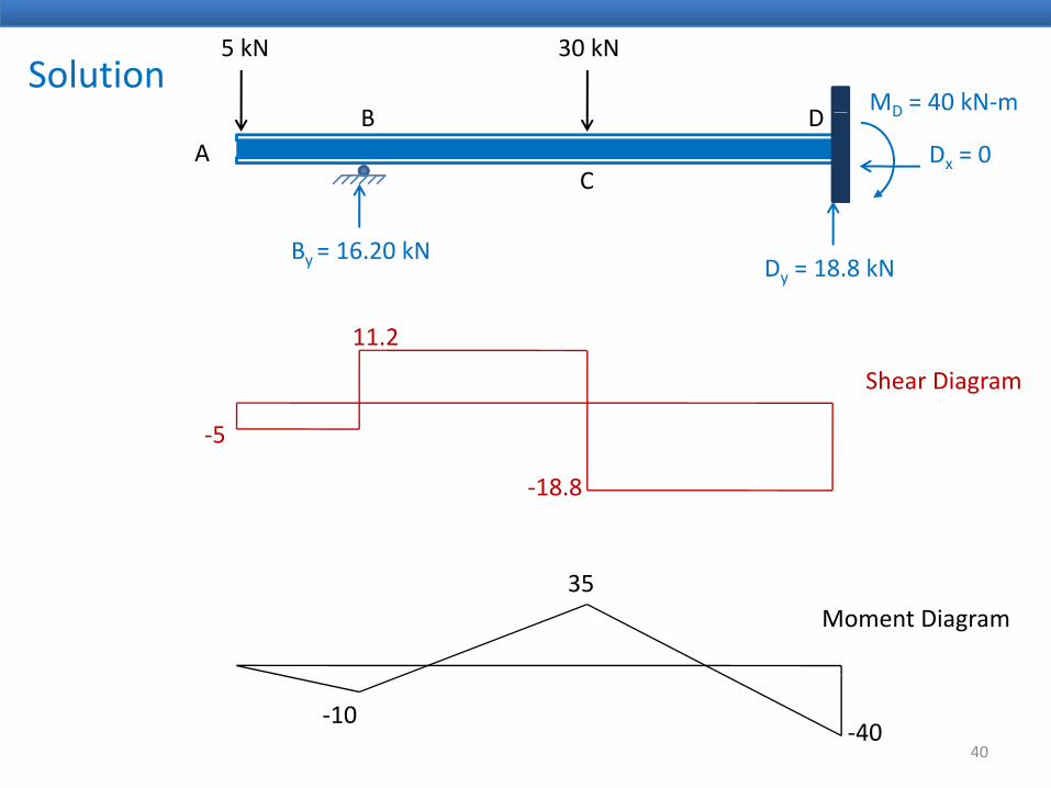
By = 16.20 kNDy = 18.8 kN
11 2
‐5
Shear Diagram
11.2
‐18.8
Moment Diagram35
40
‐10‐40
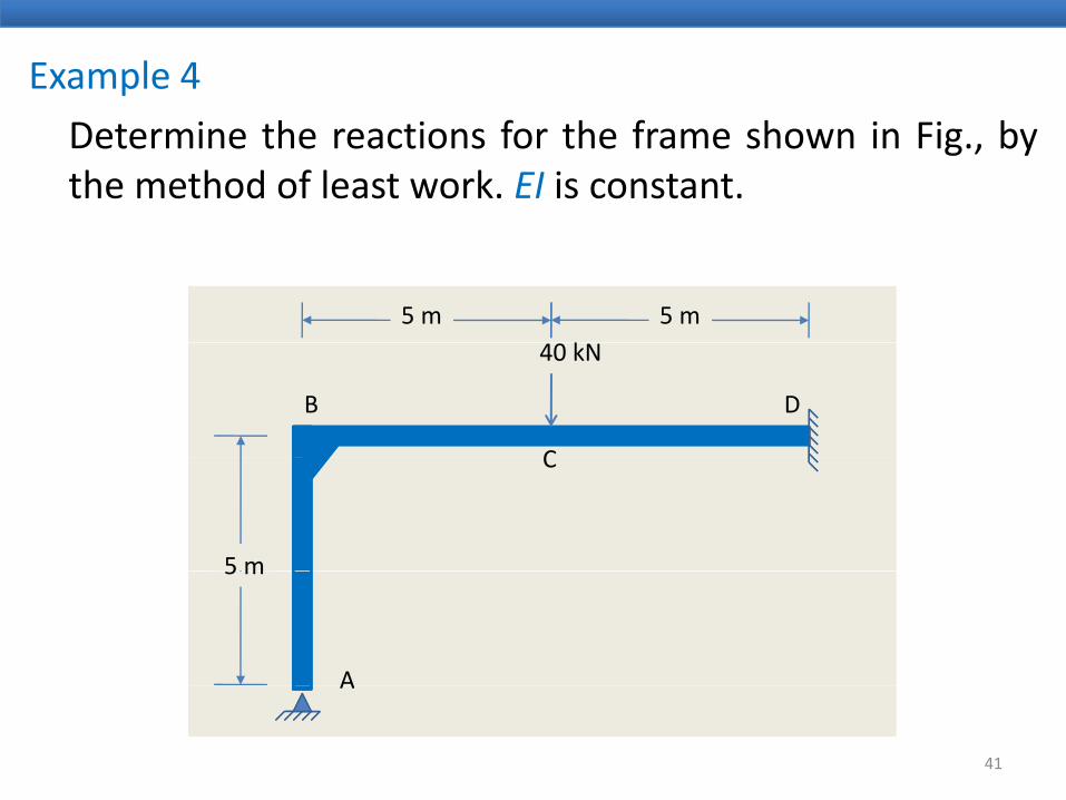
Example 4
Determine the reactions for the frame shown in Fig., bythe method of least work. EI is constant.
5 mk
5 m
B
40 kN
C
D
5 m
C
5 m
A
41
A

Solution
The structure is indeterminate to the 2nd degree. It hastwo redundant reactions.
40 kN
B
C
DHD
VD
MD
AR2
42
R1
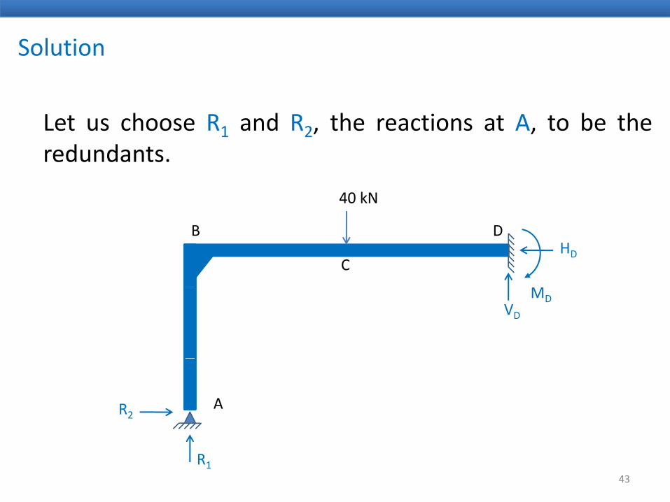
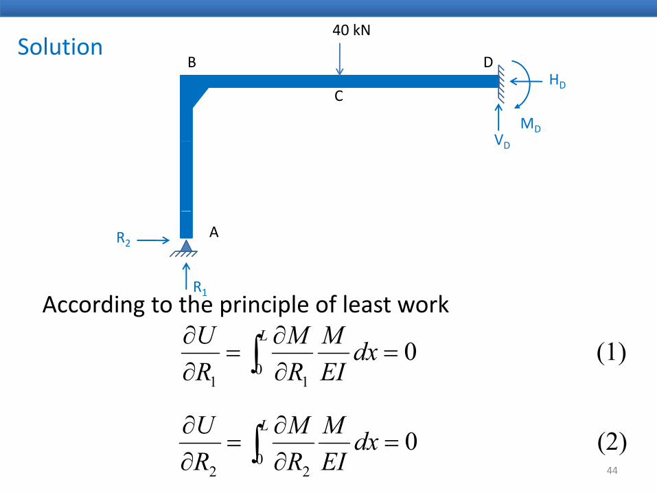
Solution
Let us choose R1 and R2, the reactions at A, to be theredundants.
40 kN
B
C
DHD
VD
MD
AR2
43
R1
SolutionB
40 kN
D
C
V
HD
MDVD
A
R
R2
According to the principle of least workR1
(1)0dxMMU L
∫ =∂
=∂ (1) 0
011
dxEIRR ∫ =
∂=
∂
MMU L ∂∂
44
(2) 00
22
dxEIM
RM
RU L
∫ =∂∂
=∂∂

SolutionB
40 kN
D
C
V
HD
MDVD
A
R
R2
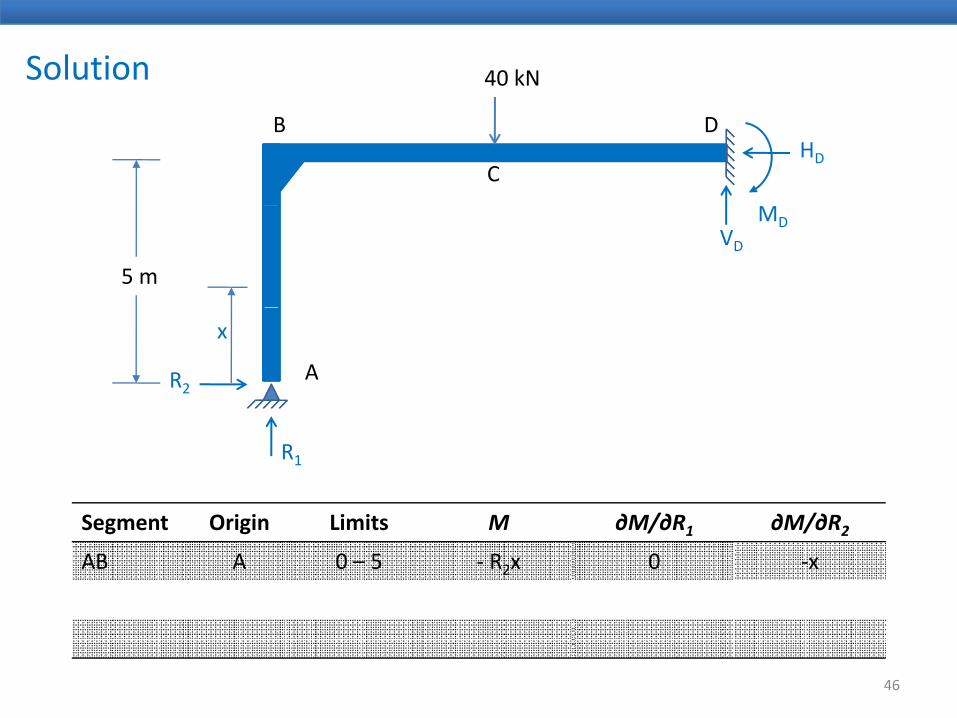
The expressions for moment and its derivative needed to
R1
psolve Eq. (1) & (2) are listed in the table on next slide.
45
Solution 40 kN
B
C
DHD
VD
MD
5 m
AR2
x
R1
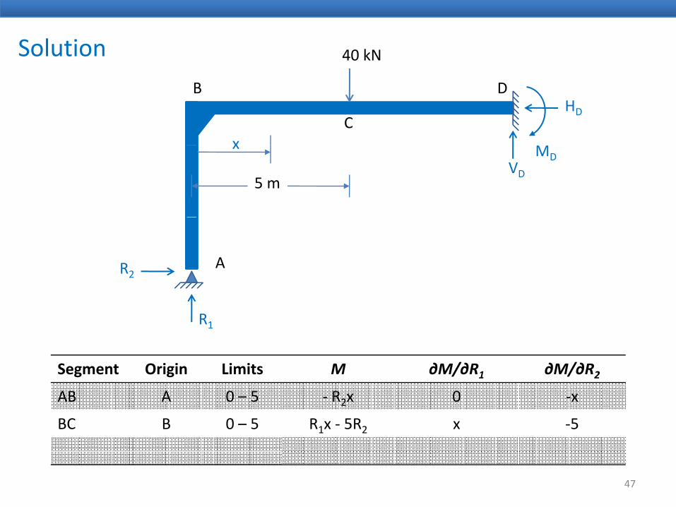
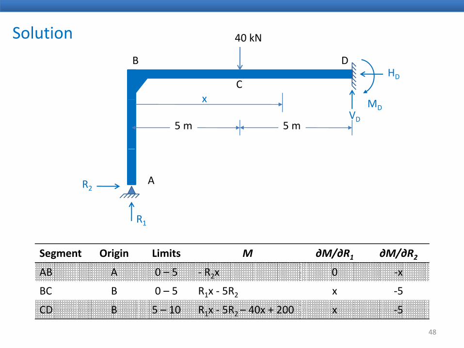
/ /Segment Origin Limits M ∂M/∂R1 ∂M/∂R2
AB A 0 – 5 ‐ R2x 0 ‐x
46
Solution 40 kN
B
C
DHD
x
VD
MDx
5 m
AR2
R1
/ /Segment Origin Limits M ∂M/∂R1 ∂M/∂R2
AB A 0 – 5 ‐ R2x 0 ‐x
BC B 0 – 5 R1x ‐ 5R2 x ‐5
47
Solution 40 kN
B
C
DHD
x
VD
MDx
5 m 5 m
AR2
R1
/ /Segment Origin Limits M ∂M/∂R1 ∂M/∂R2
AB A 0 – 5 ‐ R2x 0 ‐x
BC B 0 – 5 R1x ‐ 5R2 x ‐5
48
CD B 5 – 10 R1x ‐ 5R2 – 40x + 200 x ‐5
Solution
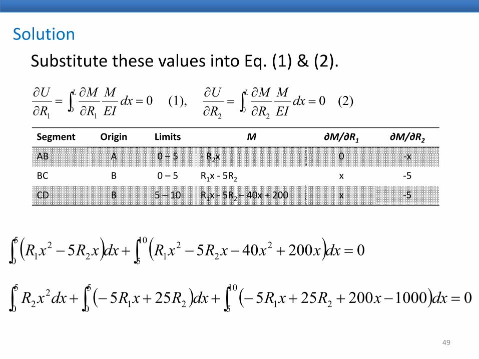
Substitute these values into Eq. (1) & (2).
(1)0dxMMU L
∫ =∂
=∂ (2)0dxMMU L
∫ =∂
=∂(1), 0
011
dxEIRR ∫ =
∂=
∂(2) 0
022
dxEIRR ∫ =
∂=
∂
Segment Origin Limits M ∂M/∂R1 ∂M/∂R2
AB A 0 5 R 0AB A 0 – 5 ‐ R2x 0 ‐x
BC B 0 – 5 R1x ‐ 5R2 x ‐5
CD B 5 – 10 R1x ‐ 5R2 – 40x + 200 x ‐5
( ) ( )∫∫ =+−−+−10 2
22
1
5
22
1 02004055 dxxxxRxRdxxRxR( ) ( )∫∫ 5 210 21
( ) ( )∫∫∫ =−++−++−+10
5 21
5
0 21
5
0
22 01000200255255 dxxRxRdxRxRdxxR
49
∫∫∫ 500

Solution
From which
04167250333 21 =−− RR0250029225004167250333
21
21
=++− RRRR
and
ANS06ANS 0.171
kNRkNR =
ANS 0.62 kNR =
50
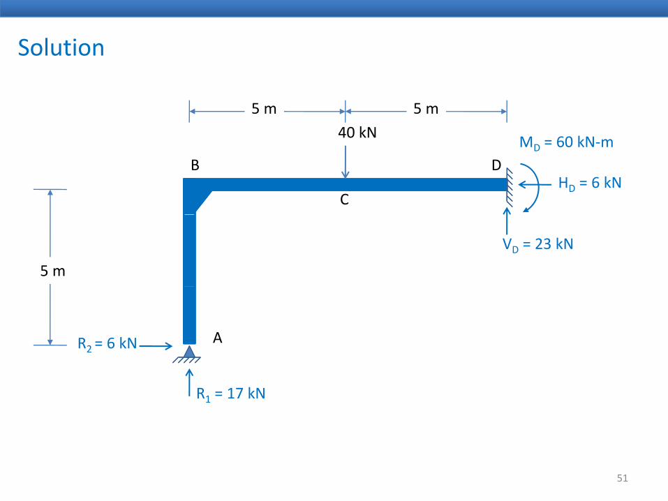
Solution
40 kN M = 60 kN‐m
5 m5 m
B
C
DHD = 6 kN
MD = 60 kN‐m
VD = 23 kN
5 m
AR2 = 6 kN
R1 = 17 kN
51
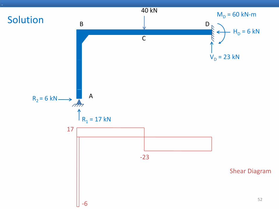
Solution
-
B
40 kN
DH 6 kN
MD = 60 kN‐m
C
VD = 23 kN
HD = 6 kN
D
A
R = 17 kN
R2 = 6 kN
R1 = 17 kN
17
Shear Diagram
‐23
52‐6
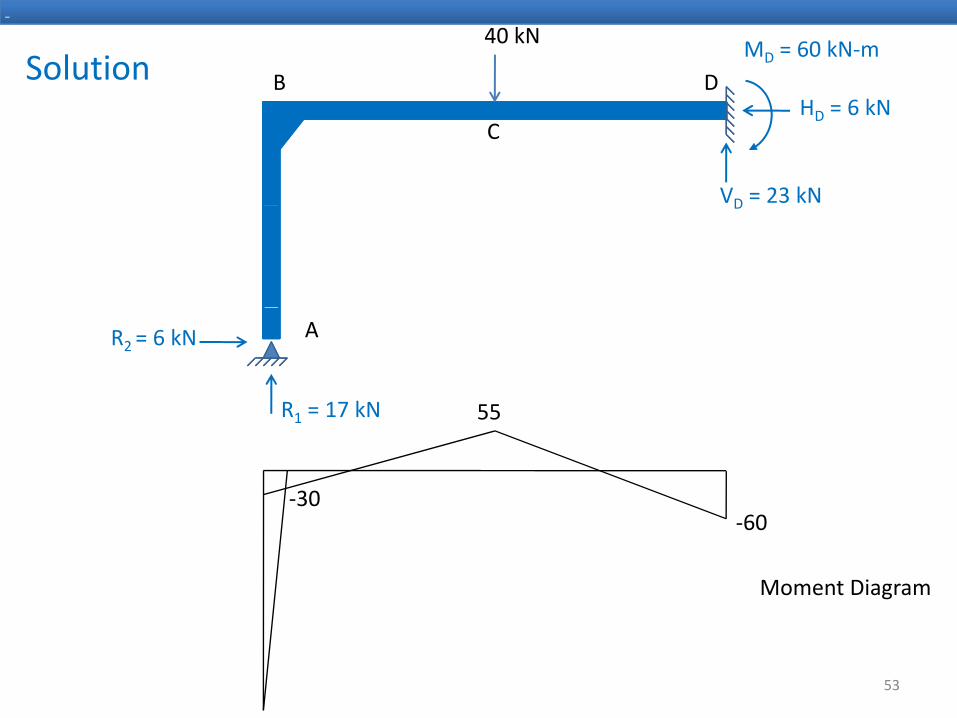
Solution
-
B
40 kN
DH 6 kN
MD = 60 kN‐m
C
VD = 23 kN
HD = 6 kN
D
A
R = 17 kN
R2 = 6 kN
55R1 = 17 kN
‐30
55
Moment Diagram
‐60
53

Example 5
University of Engineering & Technology, Taxila
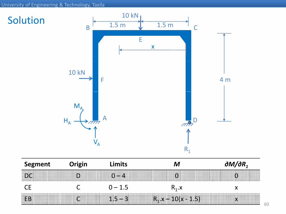
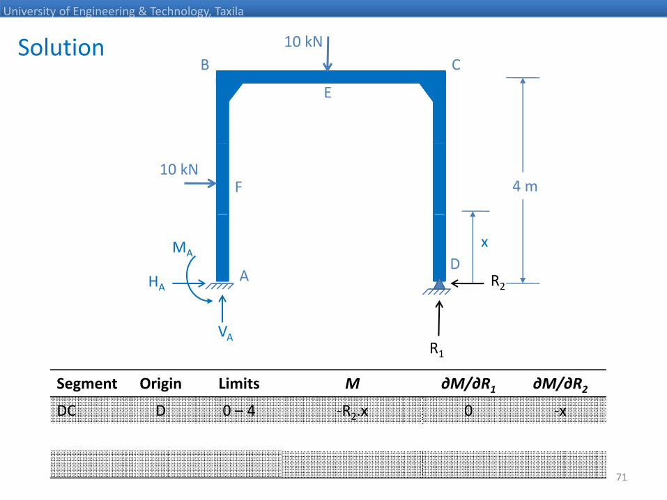
Determine the reactions for the frame shown in Fig., bythe method of least work. EI is constant.
B10 kN
C
E
2 m
10 kNF
2 m
DA
54
1.5 m 1.5 m
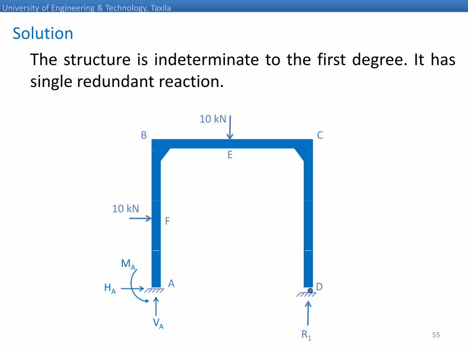
Solution
University of Engineering & Technology, Taxila
The structure is indeterminate to the first degree. It hassingle redundant reaction.
B10 kN
C
E
10 kNF
DAHA
MA
55R1
VA

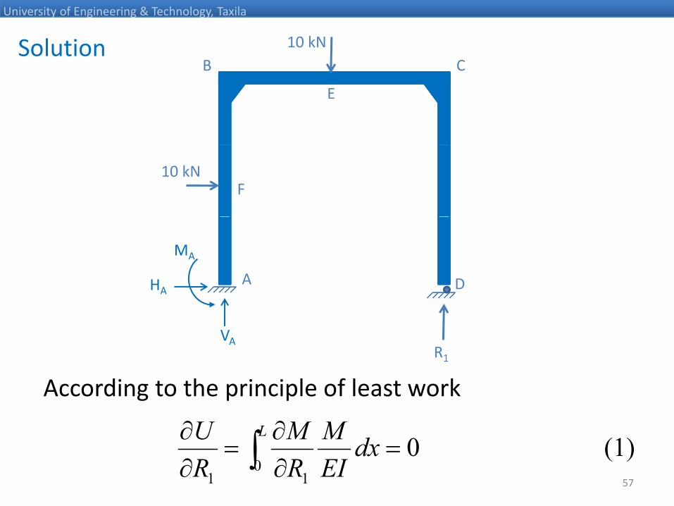
Solution
University of Engineering & Technology, Taxila
Let us choose R1, the reaction at D, to be the redundant.
B10 kN
C
E
10 kNF
DAHA
MA
56R1
VA
Solution
University of Engineering & Technology, Taxila
B10 kN
C
E
10 kNF
DAHA
MA
D
R1
VA
HA
According to the principle of least work
MMU L
∫∂∂
1
57
(1) 00
11
dxEIM
RM
RU L
∫ =∂∂
=∂∂

Solution
University of Engineering & Technology, Taxila
B10 kN
C
E
10 kNF 4 m
DAHA
MAx
D
R1
VA
HA
1
Segment Origin Limits M ∂M/∂R1
DC D 0 – 4 0 0
58
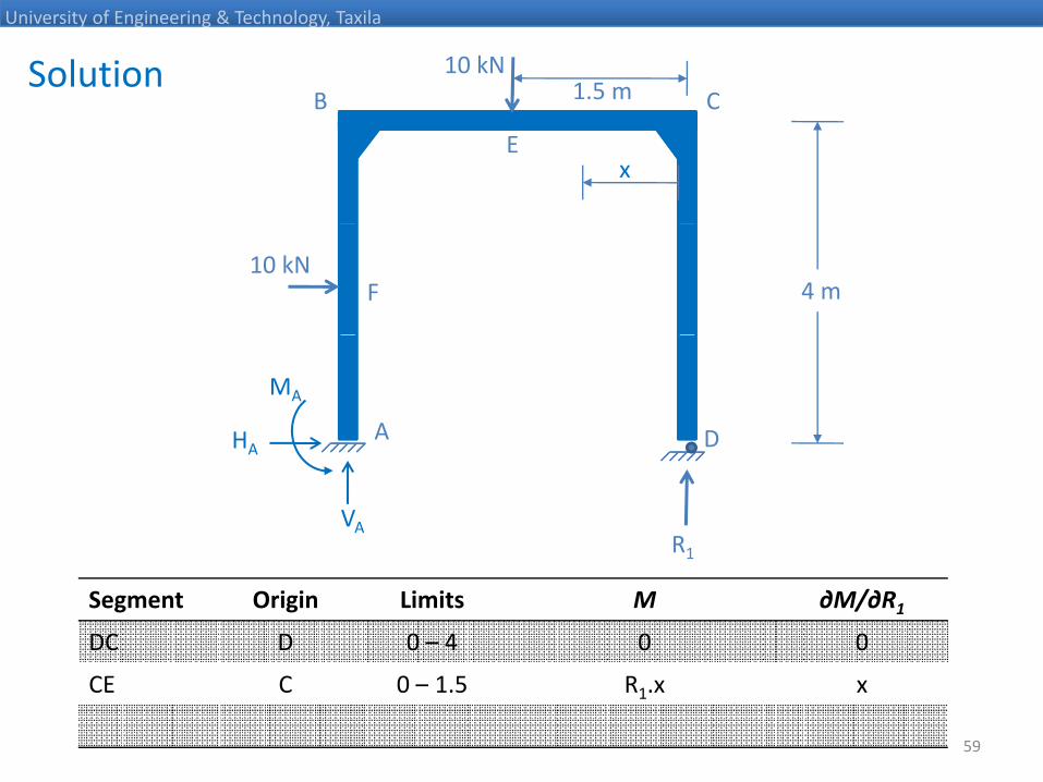
Solution
University of Engineering & Technology, Taxila
B10 kN
C1.5 m
Ex
10 kNF 4 m
DAHA
MA
D
R1
VA
HA
1
Segment Origin Limits M ∂M/∂R1
DC D 0 – 4 0 0
59
CE C 0 – 1.5 R1.x x
Solution
University of Engineering & Technology, Taxila
B
10 kN
C1.5 m1.5 m
Ex
10 kNF 4 m
DAHA
MA
D
R1
VA
HA
1
Segment Origin Limits M ∂M/∂R1
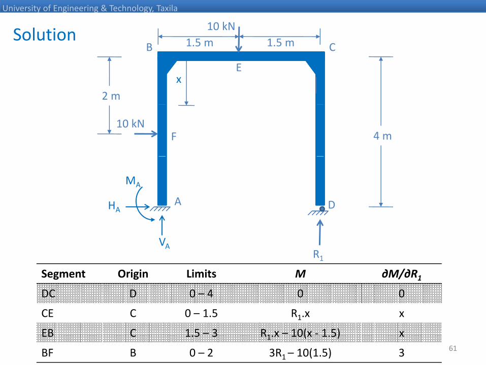
DC D 0 – 4 0 0
60
CE C 0 – 1.5 R1.x x
EB C 1.5 – 3 R1.x – 10(x ‐ 1.5) x
Solution
University of Engineering & Technology, Taxila
B
10 kN
C1.5 m1.5 m
Ex
2 m
10 kNF 4 m
DAHA
MA
D
R1
VA
HA
1
Segment Origin Limits M ∂M/∂R1
DC D 0 – 4 0 0
CE C 0 1 5 R x x
61
CE C 0 – 1.5 R1.x x
EB C 1.5 – 3 R1.x – 10(x ‐ 1.5) x
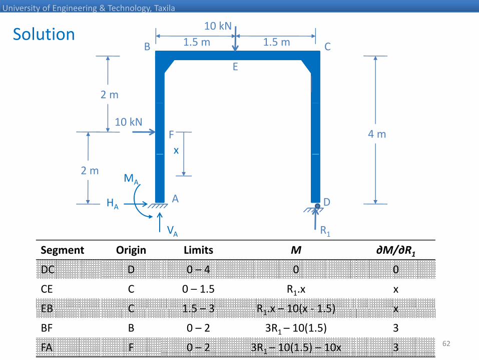
BF B 0 – 2 3R1 – 10(1.5) 3
Solution
University of Engineering & Technology, Taxila
B
10 kN
C1.5 m1.5 m
E
2 m
10 kNF 4 mx
DAHA
MA2 m
D
R1VA
HA
Segment Origin Limits M ∂M/∂R1
DC D 0 – 4 0 0
CE C 0 – 1.5 R1.x x
EB C 1 5 – 3 R x – 10(x 1 5) x
62
EB C 1.5 – 3 R1.x – 10(x ‐ 1.5) x
BF B 0 – 2 3R1 – 10(1.5) 3
FA F 0 – 2 3R1 – 10(1.5) – 10x 3

Solution
University of Engineering & Technology, Taxila
Segment Origin Limits M ∂M/∂R1
DC D 0 – 4 0 0
CE C 0 – 1.5 R1.x x1
EB C 1.5 – 3 R1.x – 10(x ‐ 1.5) x
BF B 0 – 2 3R1 – 10(1.5) 3
FA F 0 2 3R 10(1 5) 10x 3FA F 0 – 2 3R1 – 10(1.5) – 10x 3
( )[ ] ( ) ( )∫∫∫∫ ++++220.35.1 2 03045914591151011 dRdRdRdR ( )[ ] ( ) ( )∫∫∫∫ =−−+−++−+
0 10 15.1 10
21 0304594591510 dxxR
EIdxR
EIxdxxR
EIdxxR
EI
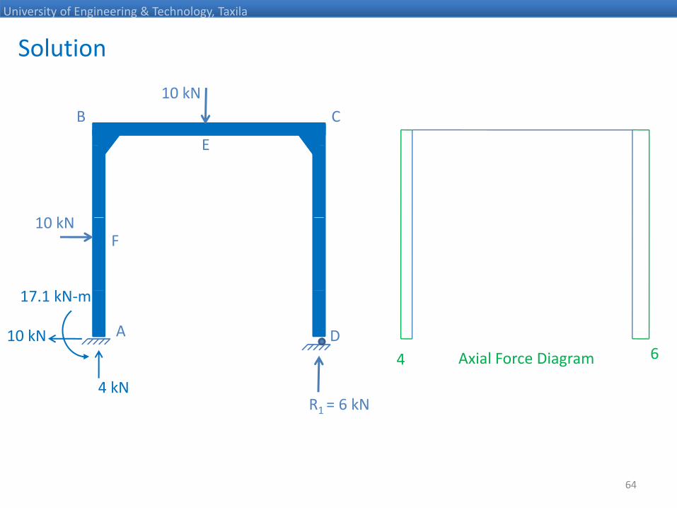
kNkNR 6958.51 ≅= kNkNR 6 958.51 ≅
63
Solution
University of Engineering & Technology, Taxila
B10 kN
C
E
10 kN
E
10 kNF
k
DA10 kN
17.1 kN‐m
4 6Axial Force Diagram
R1 = 6 kN4 kN
4 Axial Force Diagram
64

Solution
University of Engineering & Technology, Taxila
B10 kN
C
E
4
10 kN
E6
10 kNF
k
DA10 kN
17.1 kN‐m
10 Shear Force Diagram
R1 = 6 kNVA = 4 kN
10 Shear Force Diagram
65
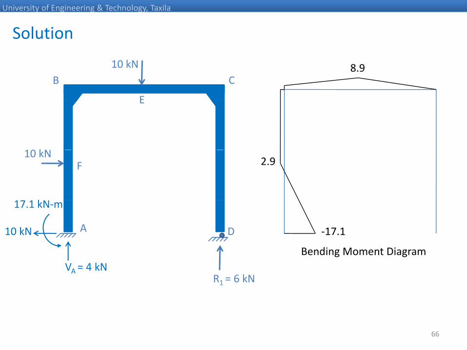
Solution
University of Engineering & Technology, Taxila
B10 kN
C
E
8.9
10 kN
E
10 kNF
k
2.9
DA10 kN
17.1 kN‐m
‐17.1
Bending Moment Diagram
R1 = 6 kNVA = 4 kN
Bending Moment Diagram
66
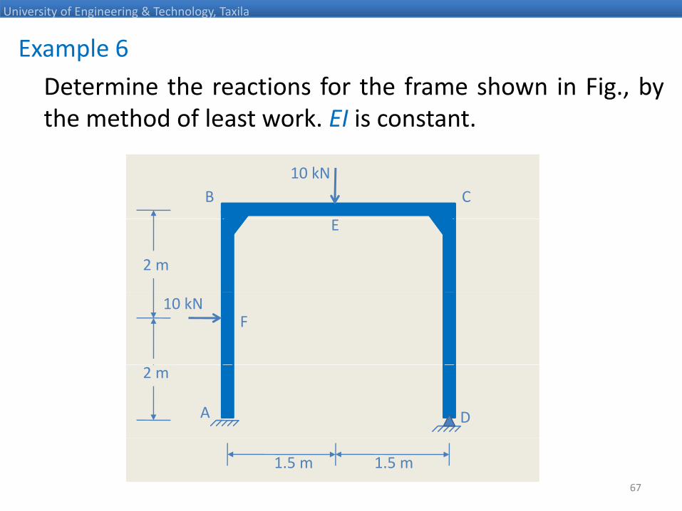
Example 6
University of Engineering & Technology, Taxila
Determine the reactions for the frame shown in Fig., bythe method of least work. EI is constant.
B10 kN
C
E
2 m
10 kNF
2 m
DA
67
1.5 m 1.5 m
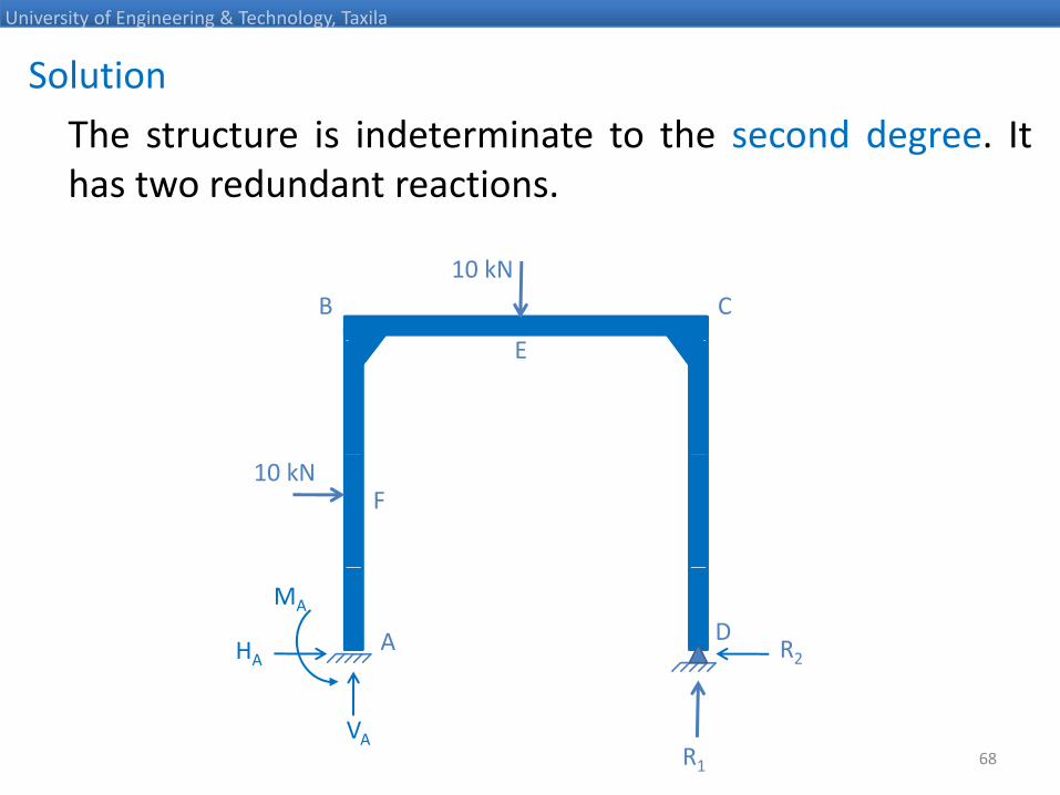
Solution
University of Engineering & Technology, Taxila
The structure is indeterminate to the second degree. Ithas two redundant reactions.
B10 kN
C
E
10 kNF
DAHA
MA
R2
68R1
VA

Solution
University of Engineering & Technology, Taxila
Let us choose R1, R2, the reaction at D, to be theredundant.
B10 kN
C
E
10 kNF
DAHA
MA
R2
69R1
VA
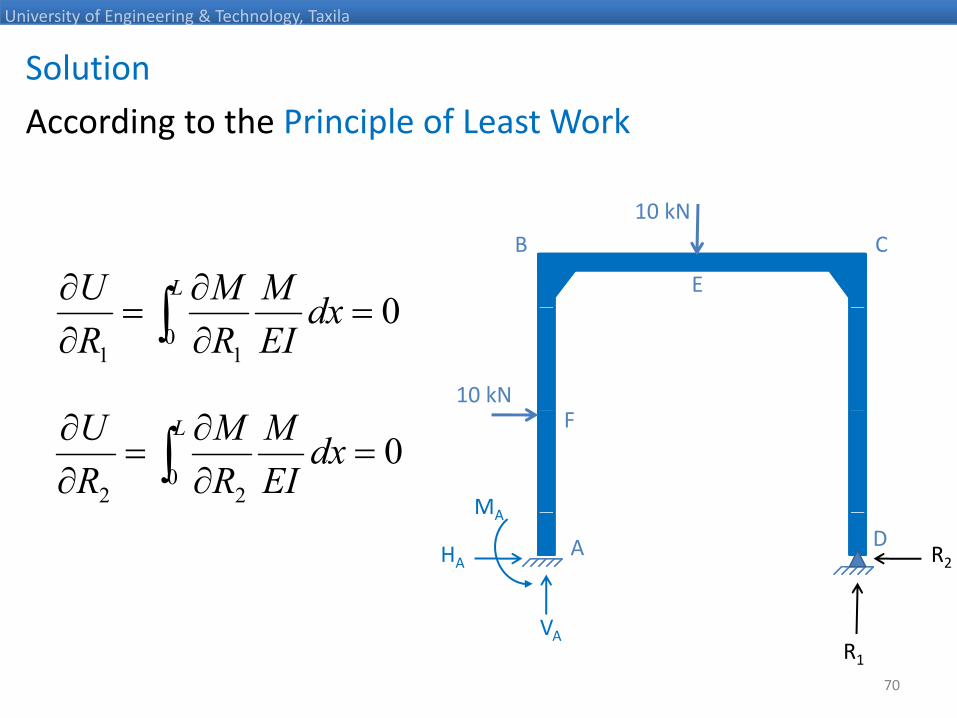
Solution
University of Engineering & Technology, Taxila
According to the Principle of Least Work
10 kNB
10 kNC
E
∫∂∂ L
dxMMU 0
10 kN
∫ =∂
=∂
dxEIRR 0
11
0
F
MA
∫ =∂∂
=∂∂ L
dxEIM
RM
RU
022
0
DAHA
MA
R2
70
R1
VA
Solution
University of Engineering & Technology, Taxila
B10 kN
C
E
10 kNF 4 m
DAHA
MAx
R2
VA
HA
R1
R2
Segment Origin Limits M ∂M/∂R1 ∂M/∂R2
DC D 0 – 4 ‐R2.x 0 ‐x
1
71

Solution
University of Engineering & Technology, Taxila
B10 kN
C1.5 m
Ex
10 kNF 4 m
DAHA
MA
R2
VA
HA
R1
R2
Segment Origin Limits M ∂M/∂R1 ∂M/∂R2
DC D 0 – 4 ‐R2.x 0 ‐x
1
72
CE C 0 – 1.5 ‐4R2 + R1.x x ‐4

Solution
University of Engineering & Technology, Taxila
B
10 kN
C1.5 m1.5 m
Ex
10 kNF 4 m
DAHA
MA
R2
VA
HA
Segment Origin Limits M ∂M/∂R ∂M/∂R
R1
R2
Segment Origin Limits M ∂M/∂R1 ∂M/∂R2
DC D 0 – 4 ‐R2.x 0 ‐x
CE C 0 – 1.5 ‐4R2 + R1.x x ‐4
73
EB C 1.5 – 3.0 ‐4R2 + R1.x ‐10(x‐1.5) x ‐4
Solution
University of Engineering & Technology, Taxila
B
10 kN
C1.5 m1.5 m
E
10 kNF 4 m
x
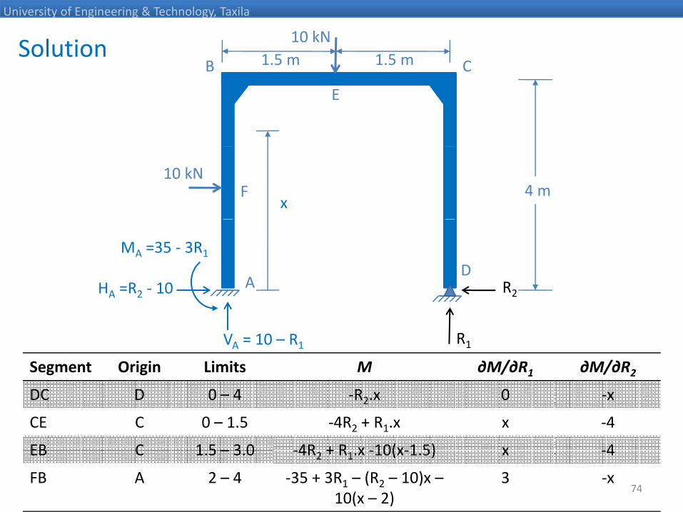
DAHA =R2 ‐ 10
MA =35 ‐ 3R1
R2
VA = 10 – R1
HA R2 10
Segment Origin Limits M ∂M/∂R ∂M/∂R
R1
R2
Segment Origin Limits M ∂M/∂R1 ∂M/∂R2
DC D 0 – 4 ‐R2.x 0 ‐x
CE C 0 – 1.5 ‐4R2 + R1.x x ‐4
74
EB C 1.5 – 3.0 ‐4R2 + R1.x ‐10(x‐1.5) x ‐4
FB A 2 – 4 ‐35 + 3R1 – (R2 – 10)x –10(x – 2)
3 ‐x
Solution
University of Engineering & Technology, Taxila
B
10 kN
C1.5 m1.5 m
E
10 kNF 4 m
DA R2
x
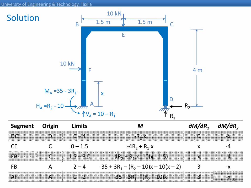
HA =R2 ‐ 10
MA =35 ‐ 3R1
Segment Origin Limits M ∂M/∂R1 ∂M/∂R2
DC D 0 4 R 0
R1
R2
VA = 10 – R1
HA R2 10
DC D 0 – 4 ‐R2.x 0 ‐x
CE C 0 – 1.5 ‐4R2 + R1.x x ‐4
EB C 1.5 – 3.0 ‐4R2 + R1.x ‐10(x ‐ 1.5) x ‐4
75
FB A 2 – 4 ‐35 + 3R1 – (R2 – 10)x – 10(x – 2) 3 ‐x
AF A 0 – 2 ‐35 + 3R1 – (R2 – 10)x 3 ‐x
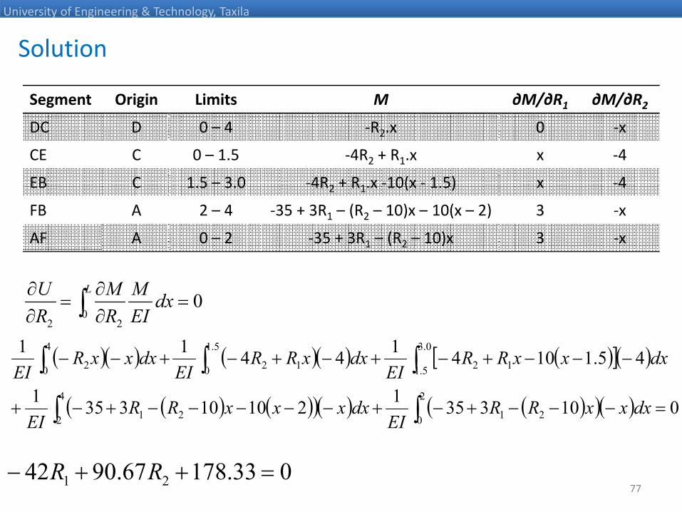
Solution
University of Engineering & Technology, Taxila
Segment Origin Limits M ∂M/∂R1 ∂M/∂R2
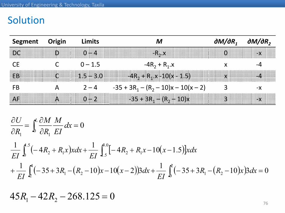
DC D 0 – 4 ‐R2.x 0 ‐x
CE C 0 – 1.5 ‐4R2 + R1.x x ‐4
EB C 1.5 – 3.0 ‐4R2 + R1.x ‐10(x ‐ 1.5) x ‐4
FB A 2 – 4 ‐35 + 3R1 – (R2 – 10)x – 10(x – 2) 3 ‐x1 2
AF A 0 – 2 ‐35 + 3R1 – (R2 – 10)x 3 ‐x
∫∂∂ L MMU
( ) ( )[ ]∫∫ −−+−++−0.3
12
5.1
12 5.1104141 xdxxxRRxdxxRR
∫ =∂∂
=∂∂ L
dxEIM
RM
RU
011
0
( ) ( )[ ]
( ) ( )( ) ( )( )∫∫
∫∫
=−−+−+−−−−+−+
+++
2
0 21
4
2 21
5.1 120 12
031033513210103351
5.11044
dxxRREI
dxxxRREI
xdxxxRREI
xdxxRREI
760125.2684245 21 =−− RR
Solution
University of Engineering & Technology, Taxila
Segment Origin Limits M ∂M/∂R1 ∂M/∂R2
DC D 0 – 4 ‐R2.x 0 ‐x
CE C 0 – 1.5 ‐4R2 + R1.x x ‐4
EB C 1.5 – 3.0 ‐4R2 + R1.x ‐10(x ‐ 1.5) x ‐4
FB A 2 – 4 ‐35 + 3R1 – (R2 – 10)x – 10(x – 2) 3 ‐x1 2
AF A 0 – 2 ‐35 + 3R1 – (R2 – 10)x 3 ‐x
∫∂∂ L MMU
( )( ) ( )( ) ( )[ ]( )∫∫∫ −−−+−+−+−+−−0.3
12
5.1
12
4
2 45.110414411 dxxxRRdxxRRdxxxR
∫ =∂∂
=∂∂ L
dxEIM
RM
RU
022
0
( )( ) ( )( ) ( )[ ]( )
( ) ( )( )( ) ( )( )( )∫∫
∫∫∫
=−−−+−+−−−−−+−+2
0 21
4
2 21
5.1 120 120 2
0103351210103351 dxxxRREI
dxxxxRREI
EIEIEI
77033.17867.9042 21 =++− RR
Solution
University of Engineering & Technology, Taxila
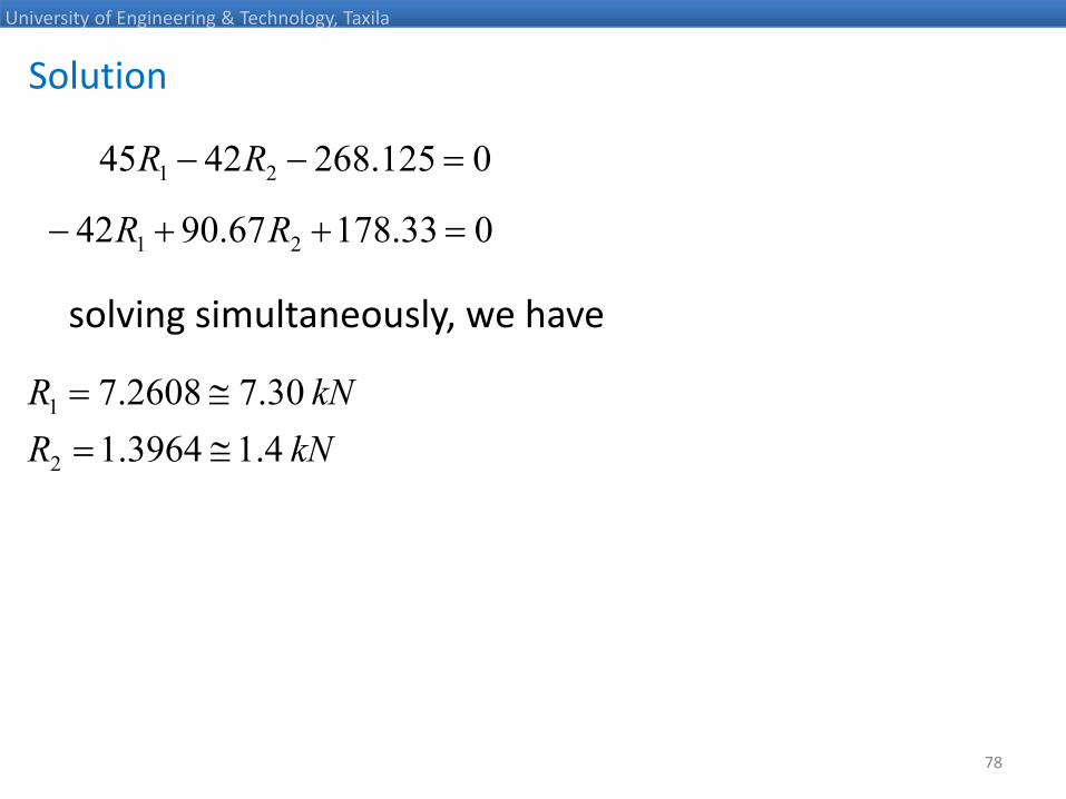
033178679042 =++ RR
0125.2684245 21 =−− RR
solving simultaneously, we have
033.17867.9042 21 =++− RR
kNRkNR
4139641 30.72608.7
2
1
≅=≅=
kNR 4.13964.12 ≅
78
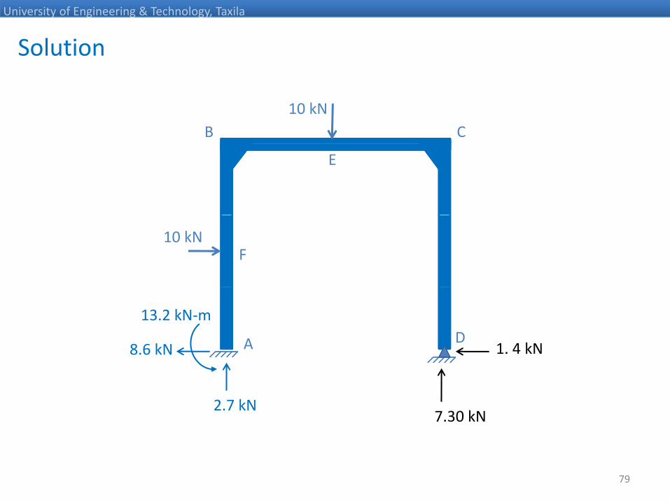
Solution
University of Engineering & Technology, Taxila
B10 kN
C
E
10 kNF
DA8.6 kN
13.2 kN‐m
1. 4 kN
7.30 kN2.7 kN
79
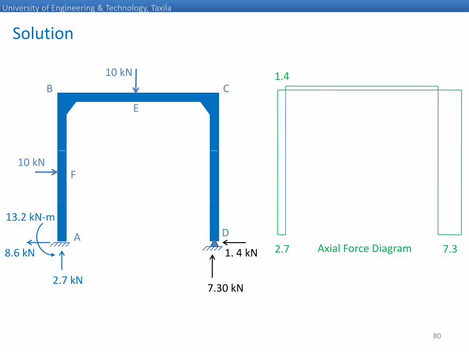
Solution
University of Engineering & Technology, Taxila
B10 kN
C1.4
E
10 kNF
2.7 7.3Axial Force DiagramDA
13.2 kN‐m
1 4 kN8 6 kN 2.7 7.3Axial Force Diagram
7.30 kN2.7 kN
1. 4 kN8.6 kN
80
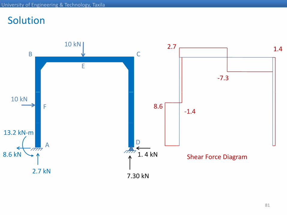
Solution
University of Engineering & Technology, Taxila
B10 kN
C2.7 1.4
E
‐7.3
10 kNF 8.6
‐1.4
DA
13.2 kN‐m
1 4 kN8 6 kN
7.30 kN2.7 kN
1. 4 kN8.6 kN Shear Force Diagram
81

Solution
University of Engineering & Technology, Taxila
B10 kN
C 1.194
5.3
E ‐5.6
10 kNF
3.983
‐13.2DA
13.2 kN‐m
1 4 kN8 6 kN Bending Moment Diagram
7.30 kN2.7 kN
1. 4 kN8.6 kN
82
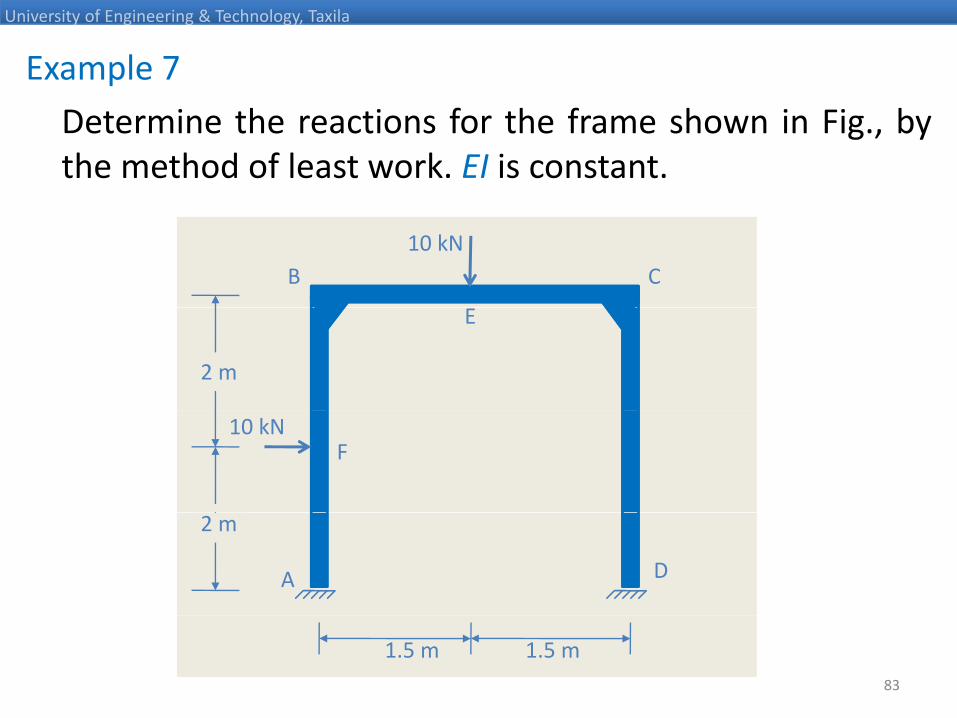
Example 7
University of Engineering & Technology, Taxila
Determine the reactions for the frame shown in Fig., bythe method of least work. EI is constant.
B10 kN
C
E
2 m
10 kNF
2 m
DA
83
1.5 m 1.5 m

Solution
University of Engineering & Technology, Taxila
The structure is determinate to the third degree. It hasthree redundant reactions.
B10 kN
C
E
2 m
10 kNF
2 m
DAHA
MA
R2
R3
84
1.5 m 1.5 mR1
VA
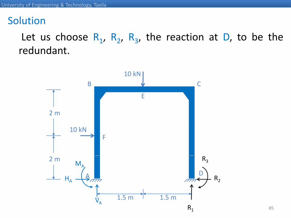
Solution
University of Engineering & Technology, Taxila
Let us choose R1, R2, R3, the reaction at D, to be theredundant.
B10 kN
C
E
2 m
10 kNF
2 m
DAHA
MA
R2
R3
85
1.5 m 1.5 mR1
VA
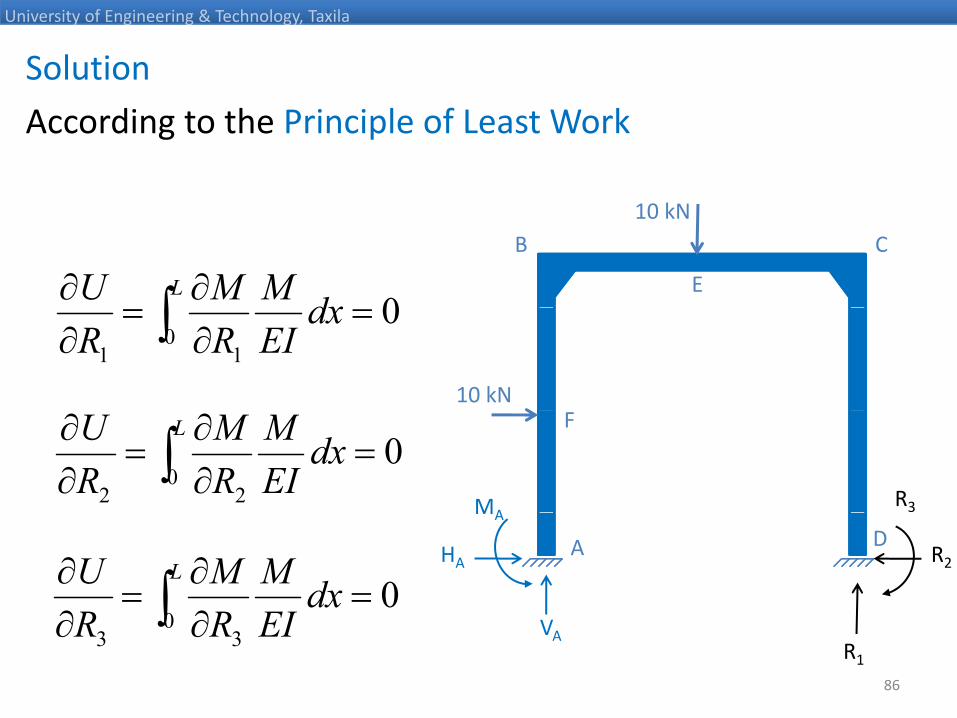
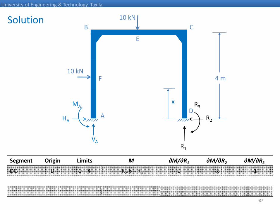
Solution
University of Engineering & Technology, Taxila
According to the Principle of Least Work
10 kNB
10 kNC
E
∫∂∂ L
dxMMU 0
10 kN
∫ =∂
=∂
dxEIRR 0
11
0
F
MA
∫ =∂∂
=∂∂ L
dxEIM
RM
RU
022
0R3
DAHA
MA
R2
∫ =∂∂
=∂∂ L
dxEIM
RM
RU
00
86
R1
VA∫ ∂∂ EIRR 0
33
Solution
University of Engineering & Technology, Taxila
B10 kN
C
E
10 kNF 4 m
DAHA
MAx
R2
R3
VA
HA
R1
R2
Segment Origin Limits M ∂M/∂R1 ∂M/∂R2 ∂M/∂R3
DC D 0 – 4 ‐R2.x ‐ R3 0 ‐x ‐1
1
87
Solution
University of Engineering & Technology, Taxila
B10 kN
C1.5 m
Ex
10 kNF 4 m
DAHA
MA
R2
R3
VA
HA
R1
R2
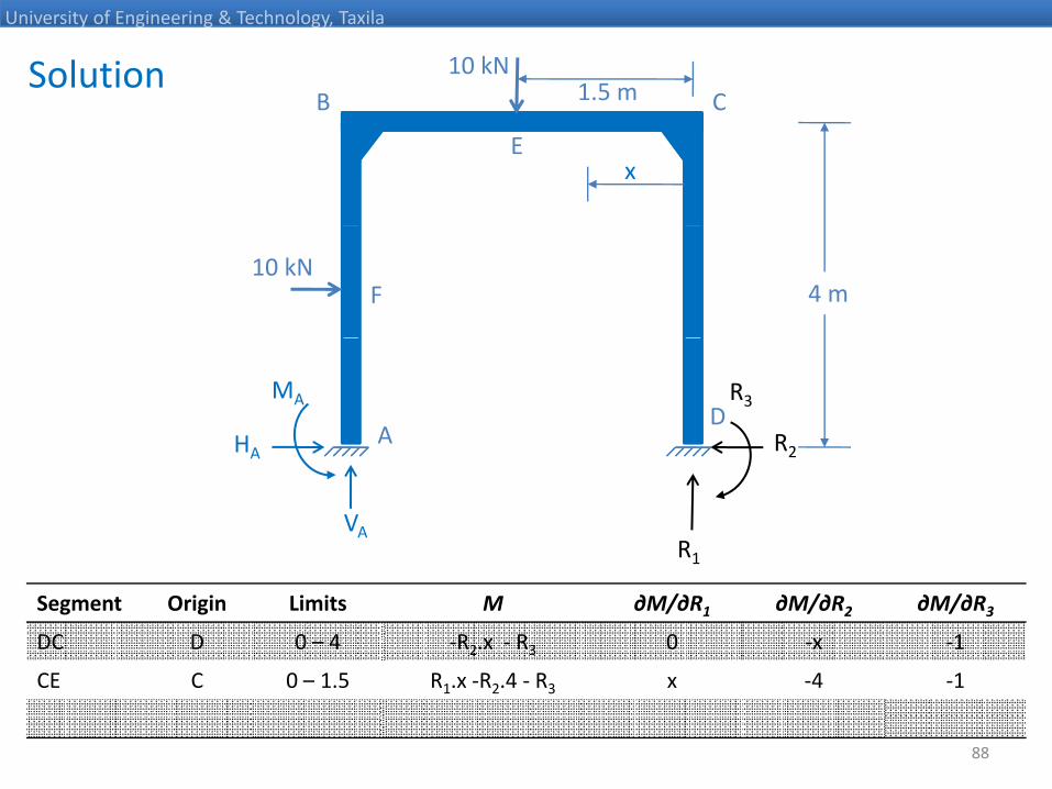
Segment Origin Limits M ∂M/∂R1 ∂M/∂R2 ∂M/∂R3
DC D 0 – 4 ‐R2.x ‐ R3 0 ‐x ‐1
CE C 0 1 5 R R 4 R 4 1
1
88
CE C 0 – 1.5 R1.x ‐R2.4 ‐ R3 x ‐4 ‐1

Solution
University of Engineering & Technology, Taxila
B
10 kN
C1.5 m1.5 m
Ex
10 kNF 4 m
DAHA
MA
R2
R3
VA
HA
R1
R2
Segment Origin Limits M ∂M/∂R1 ∂M/∂R2 ∂M/∂R3
DC D 0 – 4 ‐R2.x ‐ R3 0 ‐x ‐1
CE C 0 1 5 R R 4 R 4 1
1
89
CE C 0 – 1.5 R1.x ‐R2.4 ‐ R3 x ‐4 ‐1
EB C 1.5 – 3.0 R1.x ‐R2.4 ‐ R3 – 10(x – 1.5) x ‐4 ‐1
Solution
University of Engineering & Technology, Taxila
B
10 kN
C1.5 m1.5 m
E
10 kNF 4 m
x
DA R2
R3
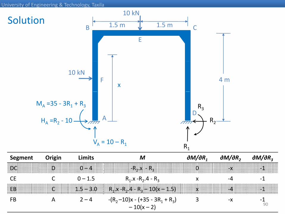
HA =R2 ‐ 10
MA =35 ‐ 3R1 + R3
R1
R2
VA = 10 – R1
HA R2 10
Segment Origin Limits M ∂M/∂R1 ∂M/∂R2 ∂M/∂R3
DC D 0 – 4 ‐R2.x ‐ R3 0 ‐x ‐1
CE C 0 – 1.5 R1.x ‐R2.4 ‐ R3 x ‐4 ‐1
90
EB C 1.5 – 3.0 R1.x ‐R2.4 ‐ R3 – 10(x – 1.5) x ‐4 ‐1
FB A 2 – 4 ‐(R2 –10)x ‐ (+35 ‐ 3R1 + R3) – 10(x – 2)
3 ‐x ‐1
Solution
University of Engineering & Technology, Taxila
B
10 kN
C1.5 m1.5 m
E
10 kNF 4 m
DA R2
R3x
HA =R2 ‐ 10
MA =35 ‐ 3R1 + R3
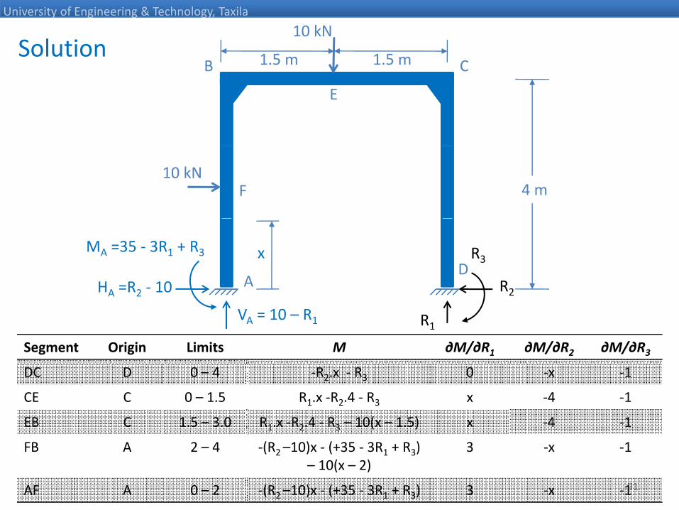
Segment Origin Limits M ∂M/∂R1 ∂M/∂R2 ∂M/∂R3
R1
R2
VA = 10 – R1
HA R2 10
DC D 0 – 4 ‐R2.x ‐ R3 0 ‐x ‐1
CE C 0 – 1.5 R1.x ‐R2.4 ‐ R3 x ‐4 ‐1
EB C 1.5 – 3.0 R1.x ‐R2.4 ‐ R3 – 10(x – 1.5) x ‐4 ‐1
91
FB A 2 – 4 ‐(R2 –10)x ‐ (+35 ‐ 3R1 + R3) – 10(x – 2)
3 ‐x ‐1
AF A 0 – 2 ‐(R2 –10)x ‐ (+35 ‐ 3R1 + R3) 3 ‐x ‐1

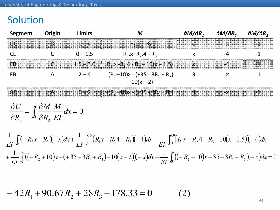
Solution
University of Engineering & Technology, Taxila
Segment Origin Limits M ∂M/∂R1 ∂M/∂R2 ∂M/∂R3
DC D 0 – 4 ‐R2.x ‐ R3 0 ‐x ‐1
CE C 0 – 1.5 R1.x ‐R2.4 ‐ R3 x ‐4 ‐1
EB C 1.5 – 3.0 R1.x ‐R2.4 ‐ R3 – 10(x – 1.5) x ‐4 ‐1
FB A 2 – 4 ‐(R2 –10)x ‐ (+35 ‐ 3R1 + R3) – 10(x – 2)
3 ‐x ‐1
( ) ( )AF A 0 – 2 ‐(R2 –10)x ‐ (+35 ‐ 3R1 + R3) 3 ‐x ‐1
∫ =∂∂
=∂∂ L
dxEIM
RM
RU
011
0
( ) ( )[ ]∫∫ −−−−+−−0.3
5.1 321
5.1
0 321 5.1104141 xdxxRRxREI
xdxRRxREI
∂∂ EIRR 11
( ) ( ) ( )( ) ( )( )∫∫ =−+−+−+−−+−+−+−+2
0 312
4
2 312 033351013210335101 dxRRxREI
dxxRRxREI
92(1) 0125.2685.164245 321 =−−− RRR
Solution
University of Engineering & Technology, Taxila
Segment Origin Limits M ∂M/∂R1 ∂M/∂R2 ∂M/∂R3
DC D 0 – 4 ‐R2.x ‐ R3 0 ‐x ‐1
CE C 0 – 1.5 R1.x ‐R2.4 ‐ R3 x ‐4 ‐1
EB C 1.5 – 3.0 R1.x ‐R2.4 ‐ R3 – 10(x – 1.5) x ‐4 ‐1
FB A 2 – 4 ‐(R2 –10)x ‐ (+35 ‐ 3R1 + R3) – 10(x – 2)
3 ‐x ‐1
( ) ( )AF A 0 – 2 ‐(R2 –10)x ‐ (+35 ‐ 3R1 + R3) 3 ‐x ‐1
∫ =∂∂
=∂∂ L
dxEIM
RM
RU
022
0
( )( ) ( )( ) ( )[ ]( )∫∫∫ −−−−−+−−−+−−−0.3
5.1 321
5.1
0 321
4
0 32 45.110414411 dxxRRxREI
dxRRxREI
dxxRxREI
∂∂ EIRR 22
( ) ( ) ( )( )( ) ( )( )( )∫∫ =−−+−+−+−−−+−+−+−+2
0 312
4
2 312 0335101210335101 dxxRRxREI
dxxxRRxREI
93(2) 033.1782867.9042 321 =+++− RRR
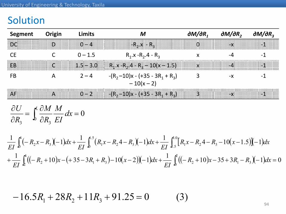
Solution
University of Engineering & Technology, Taxila
Segment Origin Limits M ∂M/∂R1 ∂M/∂R2 ∂M/∂R3
DC D 0 – 4 ‐R2.x ‐ R3 0 ‐x ‐1
CE C 0 – 1.5 R1.x ‐R2.4 ‐ R3 x ‐4 ‐1
EB C 1.5 – 3.0 R1.x ‐R2.4 ‐ R3 – 10(x – 1.5) x ‐4 ‐1
FB A 2 – 4 ‐(R2 –10)x ‐ (+35 ‐ 3R1 + R3) – 10(x – 2)
3 ‐x ‐1
( ) ( )AF A 0 – 2 ‐(R2 –10)x ‐ (+35 ‐ 3R1 + R3) 3 ‐x ‐1
∫ =∂∂
=∂∂ L
dxEIM
RM
RU
033
0
( )( ) ( )( ) ( )[ ]( )∫∫∫ −−−−−+−−−+−−−0.3
5.1 321
5.1
0 321
4
0 32 15.1104114111 dxxRRxREI
dxRRxREI
dxRxREI
∂∂ EIRR 33
( ) ( ) ( )( )( ) ( )( )( )∫∫ =−−+−+−+−−−+−+−+−+2
0 312
4
2 312 013351011210335101 dxRRxREI
dxxRRxREI
94(3) 025.9111285.16 321 =+++− RRR
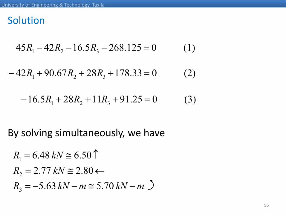
Solution
University of Engineering & Technology, Taxila
(1) 0125.2685.164245 321 =−−− RRR
(2) 033.1782867.9042 321 =+++− RRR
(3) 025.9111285.16 321 =+++− RRR
By solving simultaneously, we have
kNR ↑≅ 506486
kNkNRkNRkNR
≅←≅=↑≅=
705635 80.2 77.2
50.6 48.6
2
1
95
mkNmkNR −≅−−= 70.5 63.53
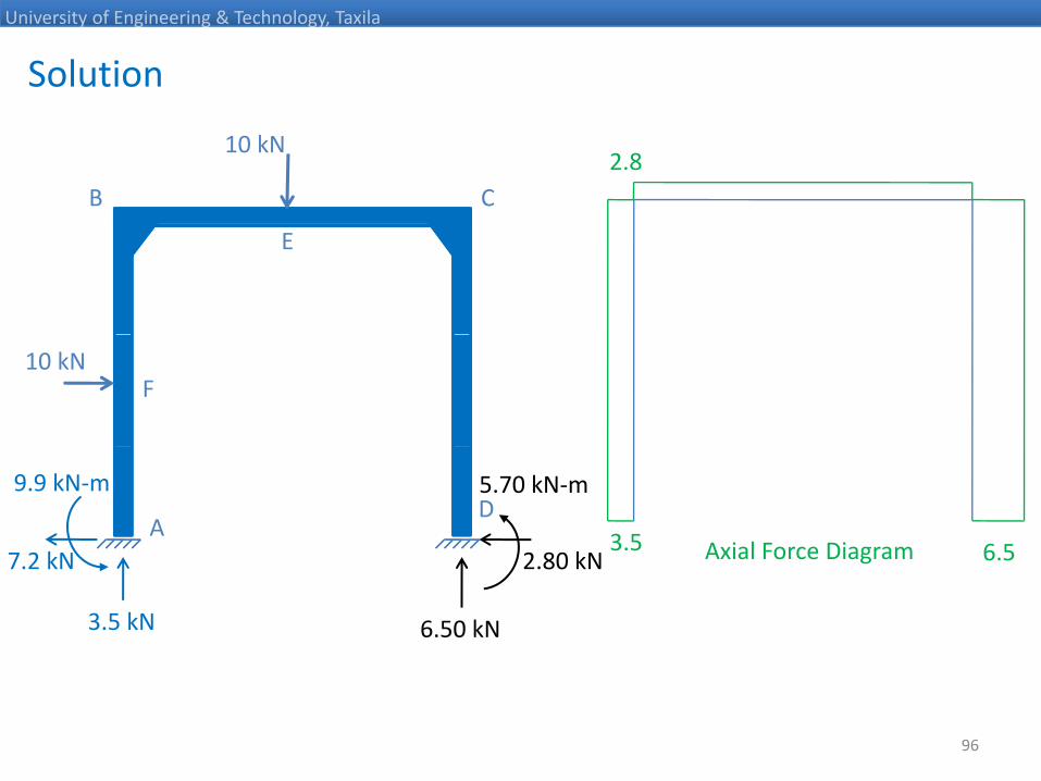
Solution
University of Engineering & Technology, Taxila
B
10 kN
C2.8
E
10 kNF
DA
2 80 kN
5.70 kN‐m
7 2 kN
9.9 kN‐m
3.5 6.5Axial Force Diagram
6.50 kN
2.80 kN
3.5 kN
7.2 kN 6.5Axial Force Diagram
96
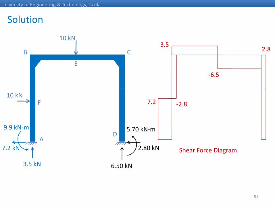
Solution
University of Engineering & Technology, Taxila
3.52.8B
10 kN
C
‐6.5
E
7.2 ‐2.810 kN
F
DA
2 80 kN
5.70 kN‐m
7 2 kN
9.9 kN‐m
Shear Force Diagram
6.50 kN
2.80 kN
3.5 kN
7.2 kN
97

Solution
University of Engineering & Technology, Taxila
B
10 kN
C
4.3
1E ‐5.5‐1
10 kNF
4.5
‐9.9D
A2 80 kN
5.70 kN‐m
7 2 kN
9.9 kN‐m
‐5.7Bending Moment Diagram
6.50 kN
2.80 kN
3.5 kN
7.2 kN
98