method to predict long time span of scour … · 1 method to predict long time span of scour around...

1

METHOD TO PREDICT LONG TIME SPAN OF SCOUR AROUND OFFSHORE WIND TURBINE FOUNDATIONS

Martin Dixen1, Iris P. Lohmann2 and Erik D. Christensen3

A new method to predict scour development around offshore structures has been developed. The method has been

tested on a monopile. The method consists of table of scour rates, which is used to predict the scour development

around the structure at different stages of the scour hole. The scour rate tables have been made based on full 3D

numerical simulations of the flow and sediment transport for fixed configurations of the scour hole. When changing

the governing parameters which are causing the scour development around the structure, the erosion rate or

backfilling rate can be calculated from the mass balance of the sediment. This leads to the scour rates tables that are

used to analyses the development of the scour hole under different current conditions. The method has been tested

against experimental scour data and showed very promising results.

Keywords: scour; monopile; CFD; current; sediment transport

INTRODUCTION

The foundation of wind turbines offshore is complex and makes up to around one third of the

overall investment. A complicating factor is that the seabed consists of loose material (sand, silt),

which moves under the influence of waves and currents. This leads to the seabed changes shape

(erosion even without wind turbines, under storms, travelling bed forms, etc.) and local erosion takes

place around the individual foundations. The latter is mainly caused by local increase of the near-bed

current speed because of the structure’s presence, and by an enhanced turbulence level generated

around the structure.

A large number of offshore wind farms are being planned. Many of these will be placed on a

seabed consisting of movable material such as sand and silt at water depths between 10 and 30 m. This

is a range where the wave and current interaction with the foundation has a significant effect on the

total load (up to around 50%). Being able to predict the exact scour/erosion depth will make the

maximum load and fatigue estimations much more accurate, which can lead to simpler and cheaper

designs; e.g. without scour protection. This will reduce investments and therefore make offshore wind

turbines a more competitive and viable alternative. Scour has been studied extensively during the past

10 to 15 years. However, work on the development of scour holes over time periods in the order of

magnitude of months/years, is sparse.

The idea behind this study is to develop a new method, which can be used to estimate the scour

and backfilling of a scour hole for any given structure. In this study the structure is taken as a monopile

due to the simple geometry and due to the fact that it is the most used foundation for offshore wind

turbines. The method which has been developed in the study can easily be used for any kind of offshore

and coastal structure where the development of scour over long time spans is a major issue.

Scour Around a Monopile

Scour around slender piles in a steady current has been investigated very extensively during the

last decades. Reviews of the subject can be found in Breusers, Nicollet & Shen (1977), Dargahi (1982),

Breusers & Raudkivi (1991), Richardson & Davies (1995), Hoffmans & Verheij (1997), Whitehouse

(1998), Melville & Coleman (2000) and Sumer & Fredsøe (2002) among others.

When a monopile is placed in the marine environment, the presence of the monopile will change

the flow pattern in the immediate neighbourhood resulting in the following phenomena

1. Contraction of the flow at the side of the monopile

2. Formation of a horseshoe vortex in front of the monopile

3. Formation of lee-wake vortices at the lee-side of the monopile

4. Generation of turbulence.

These changes will increase the local sediment transport in the case of an erodible bed, resulting in

a local scour around the monopile. For current the scour starts to develop at the upstream part of the

monopile, due to the increased sediment transport under the horseshoe vortex. The eroded sediment is

initially transported around the monopile and is deposited at the lee-side. As the scour continues to

develop the scour depth at the upstream side of the monopile increases and the scour hole starts to work

its way around the monopile to the lee-side. The sand which initially was deposited at the lee-side of

1 DHI, Agern Allé 5, 2970 Hørsholm, Denmark

2 DNV, Tuborg Parkvej 8, 2900 Hellerup, Denmark

3 Technical University of Denmark, Department of Mechanical Engineering, Nils Koppels Allé , Building 403, 2800 Lyngby, Denmark

COASTAL ENGINEERING 2012

2

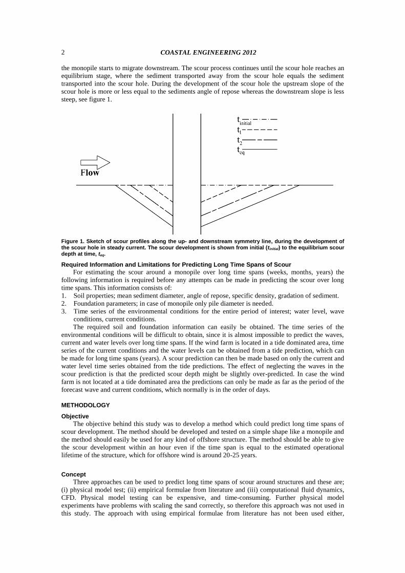
the monopile starts to migrate downstream. The scour process continues until the scour hole reaches an

equilibrium stage, where the sediment transported away from the scour hole equals the sediment

transported into the scour hole. During the development of the scour hole the upstream slope of the

scour hole is more or less equal to the sediments angle of repose whereas the downstream slope is less

steep, see figure 1.

Figure 1. Sketch of scour profiles along the up- and downstream symmetry line, during the development of the scour hole in steady current. The scour development is shown from initial (tinitial) to the equilibrium scour depth at time, teq.

Required Information and Limitations for Predicting Long Time Spans of Scour

For estimating the scour around a monopile over long time spans (weeks, months, years) the

following information is required before any attempts can be made in predicting the scour over long

time spans. This information consists of:

1. Soil properties; mean sediment diameter, angle of repose, specific density, gradation of sediment.

2. Foundation parameters; in case of monopile only pile diameter is needed.

3. Time series of the environmental conditions for the entire period of interest; water level, wave

conditions, current conditions.

The required soil and foundation information can easily be obtained. The time series of the

environmental conditions will be difficult to obtain, since it is almost impossible to predict the waves,

current and water levels over long time spans. If the wind farm is located in a tide dominated area, time

series of the current conditions and the water levels can be obtained from a tide prediction, which can

be made for long time spans (years). A scour prediction can then be made based on only the current and

water level time series obtained from the tide predictions. The effect of neglecting the waves in the

scour prediction is that the predicted scour depth might be slightly over-predicted. In case the wind

farm is not located at a tide dominated area the predictions can only be made as far as the period of the

forecast wave and current conditions, which normally is in the order of days.

METHODOLOGY

Objective

The objective behind this study was to develop a method which could predict long time spans of

scour development. The method should be developed and tested on a simple shape like a monopile and

the method should easily be used for any kind of offshore structure. The method should be able to give

the scour development within an hour even if the time span is equal to the estimated operational

lifetime of the structure, which for offshore wind is around 20-25 years.

Concept

Three approaches can be used to predict long time spans of scour around structures and these are;

(i) physical model test; (ii) empirical formulae from literature and (iii) computational fluid dynamics,

CFD. Physical model testing can be expensive, and time-consuming. Further physical model

experiments have problems with scaling the sand correctly, so therefore this approach was not used in

this study. The approach with using empirical formulae from literature has not been used either,


3

although it has shown very good predictions of scour around piles see Nielsen & Hansen (2007) and

Raaijmakers & Rudolph (2008). The reason for abandoning this approach was the lack of information

on scour for more complex structures, which would make it impossible to extend the method to more

complex structures. The approach using CFD was chosen, even though CFD calculations can be very

time-consuming especially if the entire scour development has to be simulated. Therefore, it was

decided to use CFD in a simplified way as follows. The flow around the monopile should be calculated

by CFD and the form of the scour hole should be taken as a fixed shape. This fixed shape should then

be used for simulating the scour development by using the fixed shape with different scour depths. For

each of these scour depths, a scour rate is obtained which describes how the fixed shape would move

(up/down) given a certain flow condition. By executing many simulations for all kinds of flow

conditions and different scour depths with the same fixed shape, it should be possible to set up tables

containing the flow condition and the scour rate. These tables are then used for table lookups where the

scour development rate easily and fast can be calculated by interpolation in the tables.

The Fixed Shape of the Scour Hole

By studying the shape and how the scour hole developed around a pile, a fixed shape for the scour

hole was chosen to be a frustum of a circular cone. The smallest radius, r, in the frustum was kept

constant and taken to be equal to the diameter of the monopile, see figure 2. The angle of the slope in

the frustum was taken to be equal to the sediments angle of repose, which in this study was taken to be

35 degree. By during so, the downstream angle of the slope was too steep compared to what has been

observed in experiments and from field data, see figure 2. There are several reasons not to choose a

fixed shape which fitted more correctly to the observed downstream slope of a scour hole in a constant

current. Firstly the shape should not only be valid for steady current, but also for other flow

configurations such as waves and wave-current. Secondly, the direction of marine and coastal currents

is not constant. Thirdly, the method should also be so robust that it can accommodate other types of

structures. For these more complex structures it might be difficult to know the “exact” shape of the

scour hole, so the idea was to see how well the scour predictions would be with a simple approximation

of the scour hole.

With the chosen fixed shape of the scour hole the scour depth could easily be changed, simply by

changing the height, h, of the frustum, since the slope angle and the small radius, r, was kept constant.

Figure 2. Sketch of the frustum of a circular cone, which was chosen as the fixed shape for the scour hole. The dashed line at the downstream side shows the angle of a typical downstream slope observed in model test and field data.

The CFD Flow Model

The CFD model which was used to calculate the flow around the monopile was the in-house CFD

model named NS3. NS3 is an advanced three-dimensional finite-volume Navier-Stoke solver, where

the time integrations are performed by application of the fractional step method. The model can be run

with a free surface, but it was not applied in this study. The turbulence was modelled with a k-ω, SST

(shear-stress transport) model, which was developed by Menter (1993) to improve Wilcox’s original

model so that an even higher sensitivity could be obtained for adverse-pressure-gradient flows. This is


4

a very important feature, since it is the advance-pressure-gradient that causes the boundary layer to

separate in front of the pile. The separated boundary layer subsequently rolls up to form a spiral vortex

around the pile, also known as the horseshoe vortex. As mentioned in the section Scour Around a

Monopile the horseshoe vortex plays a major role for the scouring around a monopile, and it is

therefore important that the model can capture this feature.

Sediment Transport Model

The CFD model was equipped with a sediment transport model that calculates the bed-load and

suspended sediment transport. The bed-load theory by Engelund and Fredsøe (1976) has been extended

to the case of an arbitrary sloping bed by using the vectorial approach of Kovacs and Parker (1994)

where the bed-load transport model is based on a fully nonlinear vectorial formulation for the force

balance on a sediment particle. From the vectorial force balance the following equation for the relative

velocity is obtained:

c

t

vpnμ

ktk

cθ

a

*ru

*ru

021 (1)

where ⃗ is the relative velocity vector, i.e. the difference between velocity of fluid and sediment

particle, the * implies that the given quantity is non-dimensionalised by √(g(s-1)ρ). Here g is the

acceleration of gravity, s is the relative density of sand, ρ is the density of water, a is a scaling

parameter between fluid velocity at the top of the bed-load layer and the friction velocity, θc0 is the

critical Shields parameter for initiation of sediment, ⃗ and ⃗ is the components normal and tangential

to the bed of the upwards pointing unit vector, μc is the dynamic friction factor and is a unit vector

of the direction of moving sediment particles. Eq. 1 is solved iteratively for the velocity vector of the

sediment particles:

rbp uuv (2)

where ⃗ is the near bed velocity vector. The vectorial bed-load transport, , is calculated from

*

3)1(p

b vgds

q

(3)

where ξ is the sediment content parameter, which by ways of Bagnold hypothesis reads:

sktk tvpnc

c

(4)

where is the bed shear stress vector which is obtained from the flow calculations. The suspended

sediment transport is calculated with the convection diffusion equation for suspended sediment

concentration:

z

c

z

c

y

c

y

c

x

c

x

c

z

cw

z

cw

y

cv

x

cu

t

cssss (5)

where c is concentration, t is the time, u, v and w is the velocity in x, y and z directions respectively, ws

is the fall velocity and εs is the sediment diffusion coefficient. The latter is taken to be equal to the fluid

turbulent diffusivity, νT, times a constant which is set equal to unity, i.e εs = νT.

The boundary conditions accompanying the suspended sediment concentration equation are:

At sediment free boundaries, e.g on the monopile a no-flux condition (Chauchy condition) is

imposed, i.e:

0)(

z

ccw Ts (6)

At lateral boundaries periodicity or inlet/outlet conditions are used.

At the bed boundary condition a Dirichlet conditions is used, i.e. a specification of bed

concentration c=cb(θ). In this study the Engelund-Fredsøe (1976) formula was applied.


5

Calculation of Scour Rate

The scour rate of each bed cell can be calculated from the Exner equation:

p

qf

t

hsr

bsusplb

1 (7)

where fsusp is the flux of sediment suspending or suspended sediment depositing, p is the porosity of the

sediment, hbl is the bed level measured normal to the bed and t is the time. The change in scour volume

per time is calculated by:

i

N

i

i AsrVol

0

(8)

where i is the index of the cells in the fixed scour hole, N is the total number of cells in the fixed scour

hole and Ai is the area of the i-th bed cell in the fixed scour hole. By adding the findings of Eq. 8 to the

initial volume of the fixed scour hole, Vinit, a new scour depth can be calculated. By subtracting this

new scour depth from the initial scour depth, Sinit (the height of the frustum) the change in scour depth

per time, which in this article is referred to as the scour rate of the entire scour hole, SRhole, can be

calculated for a given flow condition by:

rRRr

VolVSSR init

inithole

22

3

( 9)

where r is the radius of the monopile and R is the largest radius of the frustum, see figure 2.

Making the Scour Rate Tables

The scour rate tables have been set up for some of the most governing parameters for scour around

a pile in a steady current, which are the Shields parameter, θ, boundary layer depth to pile diameter

ratio, δ/D and the scour depth to pile diameter ratio, S/D. The procedure to obtain the scour rates which

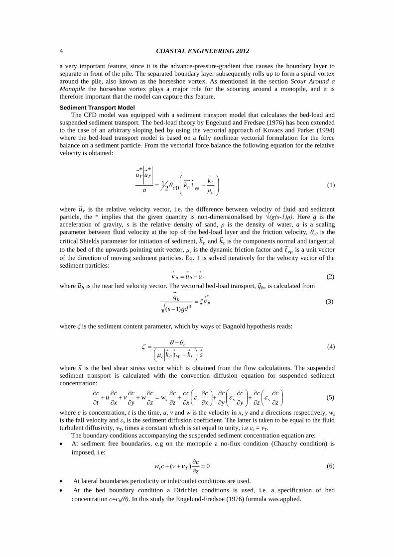
are feed into the tables was as follow. Nine grids were constructed each with a different scour depth

ranging from S/D = 0.0 to S/D=2.0, see figure 3, for each of these grids the same flow condition was

applied so the undisturbed θ value was the same in all nine simulations. The simulations were running

with a steady current. The simulations were stopped when the flow had developed and been steady for

some period of time. The scour rate, SRhole, was then calculated for each of the simulations by using Eq.

9. This procedure was applied for seven different Shields parameters, ranging from 0.04≤θ≤0.55 and

three different boundary layer depth to pile ratios, namely δ/D = 2, 3 and 4. A total of 189 simulations

were made.

Figure 3. Example of the mesh close to the monopile. The non-dimensional scour depth, S/D, is from left to right 0, 0.5, 1.0 and 1.5. (Top): Mesh seen from above. (Bottom): Mesh seen from the side.

Results

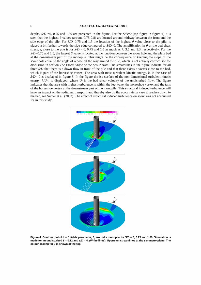
Figure 4 displays the contour of the Shields parameter and the upstream flow streamlines for the

simulation with an undisturbed Shields parameter of θ=0.12, and δ/D=4. Three non-dimensional scour


6

depths, S/D =0, 0.75 and 1.50 are presented in the figure. For the S/D=0 (top figure in figure 4) it is

seen that the highest θ values (around 0.75-0.8) are located around midway between the front and the

side edge of the pile. For S/D=0.75 and 1.5 the location of the highest θ value close to the pile, is

placed a bit further towards the side edge compared to S/D=0. The amplification in θ or the bed shear

stress, τ, close to the pile is for S/D = 0, 0.75 and 1.5 as much as 7, 3.5 and 1.3, respectively. For the

S/D=0.75 and 1.5, the largest θ value is located at the junction between the scour hole and the plain bed

at the downstream part of the monopile. This might be the consequence of keeping the slope of the

scour hole equal to the angle of repose all the way around the pile, which is not entirely correct, see the

discussion in section The Fixed Shape of the Scour Hole. The streamlines in the figure indicate for all

three S/D that there is a down-flow in front of the pile and that there exists a vortex close to the bed,

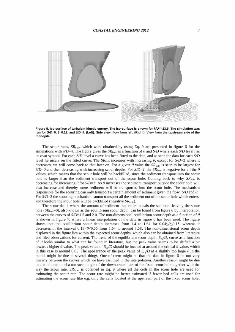
which is part of the horseshoe vortex. The area with most turbulent kinetic energy, k, in the case of

S/D= 0 is displayed in figure 5. In the figure the iso-surface of the non-dimensional turbulent kinetic

energy, k/Uf2, is displayed, where Uf is the bed shear velocity of the undisturbed flow. The figure

indicates that the area with highest turbulence is within the lee-wake, the horseshoe vortex and the tails

of the horseshoe vortex at the downstream part of the monopile. This structural induced turbulence will

have an impact on the sediment transport, and thereby also on the scour rate in case it reaches down to

the bed, see Sumer et al. (2003). The effect of structural induced turbulence on scour was not accounted

for in this study.

Figure 4. Contour plot of the Shields parameter, θ, around a monopile for S/D = 0, 0.75 and 1.50. Simulation is

made for an undisturbed θ = 0.12 and δ/D = 4. (White lines): Upstream streamlines at the symmetry plane. The

colour scaling for θ is shown at the top.


7

Figure 5. Iso-surface of turbulent kinetic energy. The iso-surface is shown for k/Uf

2=23.5. The simulation was

run for S/D=0, θ=0.12, and δ/D=4. (Left): Side view, flow from left. (Right): View from the upstream side of the

monopile.

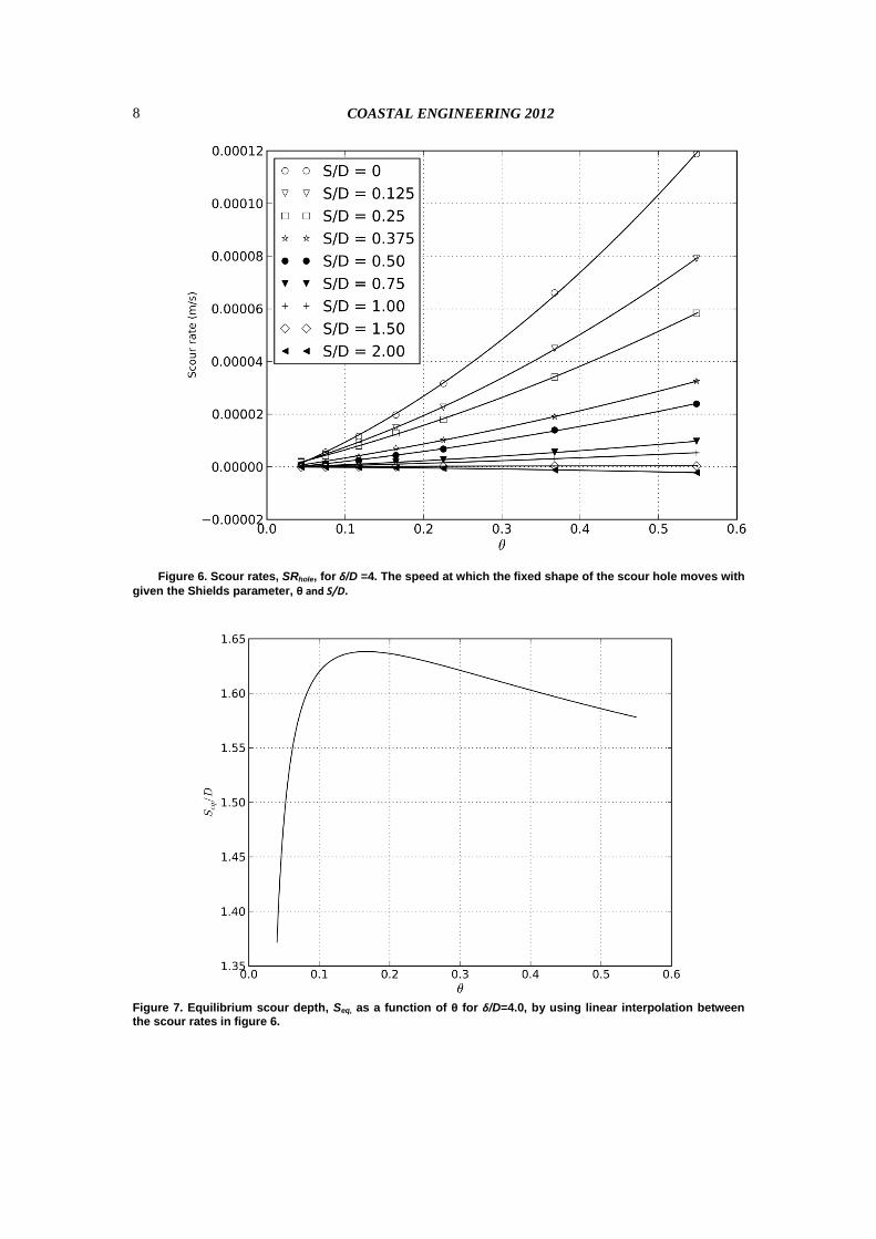
The scour rates, SRhole, which were obtained by using Eq. 9 are presented in figure 6 for the

simulations with δ/D=4. The figure gives the SRhole as a function of θ and S/D where each S/D level has

its own symbol. For each S/D level a curve has been fitted to the data, and as seen the data for each S/D

level lie nicely on the fitted curve. The SRhole increases with increasing θ, except for S/D=2 where it

decreases, we will come back to that later on. For a given θ value the SRhole is seen to be largest for

S/D=0 and then decreasing with increasing scour depths. For S/D=2, the SRhole is negative for all the θ

values, which means that the scour hole will be backfilled, since the sediment transport into the scour

hole is larger than the sediment transport out of the scour hole. Coming back to why SRhole is

decreasing for increasing θ for S/D=2: As θ increases the sediment transport outside the scour hole will

also increase and thereby more sediment will be transported into the scour hole. The mechanism

responsible for the scouring can only transport a certain amount of sediment given the flow, S/D and θ.

For S/D=2 the scouring mechanism cannot transport all the sediment out of the scour hole which enters,

and therefore the scour hole will be backfilled (negative SRhole).

The scour depth where the amount of sediment that enters equals the sediment leaving the scour

hole (SRhole=0), also known as the equilibrium scour depth, can be found from figure 6 by interpolation

between the curves of S/D=1.5 and 2.0. The non-dimensional equilibrium scour depth as a function of θ

is shown in figure 7, where a linear interpolation of the data in figure 6 has been used. The figure

shows that the equilibrium scour depth increases from 1.4 to 1.64 for 0.04≤θ≤0.15, whereas it

decreases in the interval 0.15<θ≤0.55 from 1.64 to around 1.58. The non-dimensional scour depth

displayed in the figure lies within the expected scour depths, which also can be obtained from literature

and filed observations for current. The trend of the equilibrium scour depth, Seq/D, curve as a function

of θ looks similar to what can be found in literature, but the peak value seems to be shifted a bit

towards higher θ value. The peak value of Seq/D should be located at around the critical θ value, which

in this case is around 0.05. The appearance of the peak value of Seq/D at a slightly too large θ in the

model might be due to several things. One of them might be that the data in figure 6 do not vary

linearly between the curves which we have assumed in the interpolation. Another reason might be due

to a combination of a too steep angle of the downstream part of the fixed scour hole together with the

way the scour rate, SRhole, is obtained in Eq. 9 where all the cells in the scour hole are used for

estimating the scour rate. The scour rate might be better estimated if fewer bed cells are used for

estimating the scour rate like e.g. only the cells located at the upstream part of the fixed scour hole.


8

Figure 6. Scour rates, SRhole, for δ/D =4. The speed at which the fixed shape of the scour hole moves with

given the Shields parameter, θ and S/D.

Figure 7. Equilibrium scour depth, Seq, as a function of θ for δ/D=4.0, by using linear interpolation between the scour rates in figure 6.


9

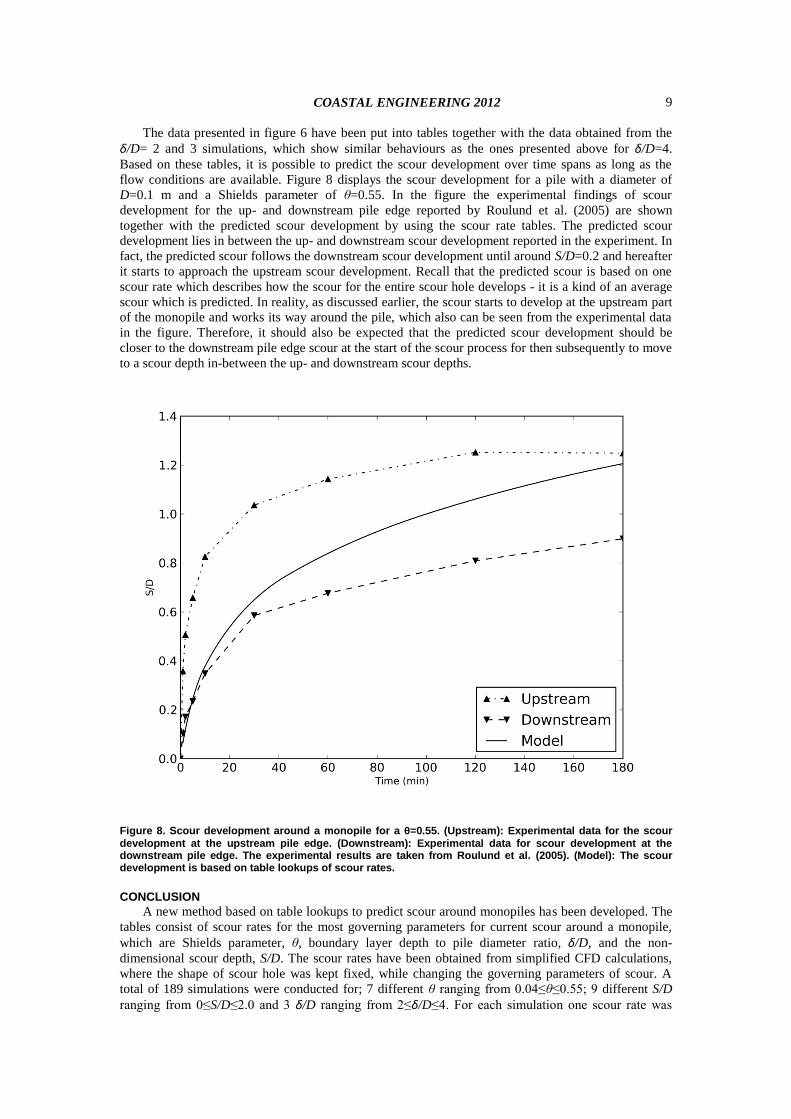
The data presented in figure 6 have been put into tables together with the data obtained from the

δ/D= 2 and 3 simulations, which show similar behaviours as the ones presented above for δ/D=4.

Based on these tables, it is possible to predict the scour development over time spans as long as the

flow conditions are available. Figure 8 displays the scour development for a pile with a diameter of

D=0.1 m and a Shields parameter of θ=0.55. In the figure the experimental findings of scour

development for the up- and downstream pile edge reported by Roulund et al. (2005) are shown

together with the predicted scour development by using the scour rate tables. The predicted scour

development lies in between the up- and downstream scour development reported in the experiment. In

fact, the predicted scour follows the downstream scour development until around S/D=0.2 and hereafter

it starts to approach the upstream scour development. Recall that the predicted scour is based on one

scour rate which describes how the scour for the entire scour hole develops - it is a kind of an average

scour which is predicted. In reality, as discussed earlier, the scour starts to develop at the upstream part

of the monopile and works its way around the pile, which also can be seen from the experimental data

in the figure. Therefore, it should also be expected that the predicted scour development should be

closer to the downstream pile edge scour at the start of the scour process for then subsequently to move

to a scour depth in-between the up- and downstream scour depths.

Figure 8. Scour development around a monopile for a θ=0.55. (Upstream): Experimental data for the scour

development at the upstream pile edge. (Downstream): Experimental data for scour development at the downstream pile edge. The experimental results are taken from Roulund et al. (2005). (Model): The scour development is based on table lookups of scour rates.

CONCLUSION

A new method based on table lookups to predict scour around monopiles has been developed. The

tables consist of scour rates for the most governing parameters for current scour around a monopile,

which are Shields parameter, θ, boundary layer depth to pile diameter ratio, δ/D, and the non-

dimensional scour depth, S/D. The scour rates have been obtained from simplified CFD calculations,

where the shape of scour hole was kept fixed, while changing the governing parameters of scour. A

total of 189 simulations were conducted for; 7 different θ ranging from 0.04≤θ≤0.55; 9 different S/D

ranging from 0≤S/D≤2.0 and 3 δ/D ranging from 2≤δ/D≤4. For each simulation one scour rate was


10

obtained which describes the speed at which the scour hole would develop. The scour rate can be seen

as an average speed at which the scour hole will develop given the initial scour depth and flow

conditions.

The method is based on a simple scour hole shape, which not totally resembles the real scour shape

around a monopile. The shape of a scour hole was taken as a frustum with side slopes equal to the

angle of repose, this is not entirely correct for the downstream slope of the scour hole which normally

is 10-15 degree less steep than the upstream slope. The purpose of choosing a shape of the scour hole

which does not entirely resemble the real scour shape was due to future perspectives of the method,

where the method should be used for more complex structures where the shape of the scour hole is not

as well-known as it is for the case of a monopile.

The scour can easily and fast be predicted by using the scour rate tables and the scour can be

predicted for time periods as far as the flow condition is known. The method has been tested against

experimental data for scour development around a pile. The predicted scour development showed very

promising results, the predicted scour development lay in between the experimental up- and

downstream scour development.

ACKNOWLEDGMENTS

This study was funded by the Danish Council for Strategic Research (DSF)/Energy and

Environment Program ''Seabed Wind Farm Interaction''

REFERENCES

Breusers, H. N. C., Nicollet, G. & Shen, H. W. 1977. Local scour around cylindrical piers. J. Hydraul.

Res. 15, 211–252.

Breusers, H. N. C. & Raudkivi, A. J. 1991. Scouring. A. A. Balkema, Rotterdam.

Dargahi, B. 1982. Local scour around bridge piers – A review of practice and theory. Bull. 114,

Hydraulics Laboratory, Royal Institute of Technology, Stockholm, Sweden.

Hoffmans, G. J. C. M. & Verheij, H. J. 1997. Scour Manual. A. A. Balkema, Rotterdam.

Kovacs, A., and Parker, G. (1994). A new vectorial bedload formulation and its application to the time

evolution of straight river channels. Journal of fluid Mechanics vol. 257, pp. 153-183

Melville, B. W. & Coleman, S. E. 2000 Bridge Scour. Water Resources, LLC, CO, USA

Menter, F. R. 1993 Zonal two equation k–ω turbulence models for aerodynamic flows. AIAA Paper

93-2906, AIAA 24th Fluid Dynamic Conference, July 6–9, 1993, Orlando, Florida.

Nielsen,. A.W. and Hansen, E.A., (2007): Time-varying wave and current-induced scour around

offshore wind turbines. Proceedings of the 26th International Conference on Offshore Mechanics

and Arctic Engineering, OMAE2007, June 10-15, 2007, San Diego, California, USA

Raaijmakers, T. and Rudolph, D. (2008): Time-dependent scour development under combined current

and waves conditions - laboratory experiments with online monitoring technique. Fourth

International Conference on scour and erosion, ICSE-4, 2008, Tokyo, Jaopan.

Richardson, E. V. & Davies, S. R. 1995 Evaluating Scour at Bridges. 3rd edn. US Department of

Transportation, HEC 18, FHWA-IP-90-017.

Roulund, A., Sumer, B.M., Fredsøe, J. and Michelsen, J. (2005). "Numerical and experimental

investigation of flow and scour around a circular pile", J. Fluid Mechanics,vol. 534, 351-401.

Sumer, B. M., Chua, L. H. C., Cheng, N.-S. Fredse, J. (2003). "The influence of turbulence on bedload

sediment transport", J. Hydraul. Engng ASCE 129(8).

Sumer, B. M. & Fredsøe, J. 1997 Hydrodynamics Around Cylindrical Structures. World Scientific.

Whitehouse, R. 1998 Scour at Marine Structures. Thomas Telford.

method to predict long time span of scour … · 1 method to predict long time span of scour around...

Documents