methodological and applicative problems of using pearson ... · methodological and applicative...
TRANSCRIPT

Romanian Statistical Review - Supplement nr. 2 / 2017148
Methodological and Applicative Problems of using Pearson Correlation Coeffi cient in the
Analysis of Socio-Economic Variables
Daniela-Emanuela Dănăcică
Faculty of Economics, Constantin Brâncuși University of Târgu-Jiu
Abstract
The aim of this paper is to focus on the methodological and applicative
problems that Pearson correlation coeffi cient may arise when used to
analyzing the relationship between socio-economic variables. Using real data
we empasized the effect of the most important factors infl uencing the size and
interpretation of Pearson coeffi cient and we presented the special cases of this
statistics and their usefulness.
Keywords: correlation, Pearson coeffi cient, size, linearity
JEL Classifi cation: C18, C01
1. Introduction
If we focus on the name of simple linear correlation coeffi cient,
known in the literature as “Pearson product-moment correlation coeffi cient”,
we could erroneously belive that the English mathematician and biostatistician
Karl Pearson developed this coeffi cient himself. In fact, it was Francis Galton
the man who fi rst conceived and formulated the concepts of correlation
and regression (Stanton, 2001). Later on, Bravais and Pearson elaborated a
rigourous mathematical approach for correlation and regression.
Pearson product-moment correlation coeffi cient is widely used in
economics, social sciences, medicine, etc., as a measure of linear relationship
between two variable X and Y. The mathematical formula for this coeffi cient
developed by Pearson in 1895 is:
� �
�
� �
�
��
��
��
�
�
�
��
�
�
�
�
��
����
����
' '
>'
'>
?;9;9@
;;99
���������������������������������������������������
�
�
(1)
Since :�� ���
����
���
�
�
� ;;99
;� ��9 '
��
��� ��/��+����, we have
���/��+����
��
���
��
��
;� ��9> � �������������������������������������������������9 (2)

Revista Română de Statistică - Supliment nr. 2 / 2017 149
therefore, as Rodgers and Nicewander (1988) underline, Pearson coeffi cient
can be described as a standardized covariance.
In statistics is widely used the following formula:
−
−
⋅−=
∑∑∑ ∑
∑∑ ∑
=== =
== =
n
i
i
n
i
i
n
i
n
i
ii
n
i
i
n
i
n
i
iii
xy
yynxxn
yxyxn
r
1
2
1
2
1 1
22
11 1/
)(
(3)
[ ]1,1/ −∈xyr . The closer the value of xyr / is to +1 or -1, the higher the
association between these two variables is; the closer the value of xyr / is to 0,
the weaker the strengh of the relationship is.
In many statistics textbooks the interval [-1, 1] is divided in subintervals;
the intensity of relationship between X and Y is interpreted depending on the
subintervals of which xyr / belongs. However, a specifi c value of Pearson
coeffi cient is difi cult to interpret. For example, it is diffi cult to interpret a
0.6 value of xyr / compared with a 0.7 value. Rinaman (1993) underlines that
there is no precise interpretation that could be attached to particular values of
Pearson correlation coeffi cient. Also, since ]1,0[/ ∈xyr there is a tendency
to mistakenly interpret its value as the proportion of identical ( ii yx , ) pairs, or
as the probability of a correct prediction (Falk and Well, 1997; Eisenbach and
Falk, 1984).
Although Pearson correlation is widely used by researchers from
many research areas and all the basic statistics textbooks cover the topic of
correlation, there are not so many studies focused on the subtle nuances of this
measure and on the atypical cases of Pearson coeffi cient and their usefulness.
Various analyzes about what is communicated using Pearson coeffi cient must
be carefully presented, because the similarities between some interpretation
are subject to specifi c constraints (Falk and Well, 1997). Each result obtained
using this statistics should be carefully checked if the intepretation is
appropriate to the used model; some interpretation of Pearson correlation
coeffi cient are valid only under certain particular circumstances.
The aim of this article is to emphasize the methodological and
applicative problems of using Pearson coeffi cient in the analysis of relationship
between socio-economic variables. Pearson coeffi cient is a versatile statistics
and it has many subtile shades. We will focus on the most important factors
affecting the value and interpretation of Pearson coeffi cient and on the
limitation of this statistics. We will discuss about particular cases when one or
both of the analyzed variables are dichotomous and we will present the special

Romanian Statistical Review - Supplement nr. 2 / 2017150
cases of Pearson coeffi cient and their particularities. To our knowledge, there
is no statistics textbooks in our country that cover aspects regarding factors
infl uencing the size and interpretation of Pearson coeffi cient, or aspects
regarding special cases of Pearson coeffi cient (other than Spearman and
Kendall coeffi cient). Thus this paper seeks to fi ll a gap in the existing literature
too.
2. Factors infl uencing the size and interpretation of Pearson correlation
coeffi cient
In this section of paper we will analyze the effect of main factors
infl uencing the size and interpretation of Pearson correlation coeffi cient.
The most important factors that have a signifi cant effect on the value and
interpretation of Pearson correlation coeffi cient are: the shape of distribution,
the size of sample, the aberrant values (outliers), the restriction of range and
nonlinearity, a third variable or more (Chen and Popovich, 2002; Goodwin
and Leech, 2006).
In every statistics textbooks it is written that Pearson correlation
coeffi cient has values within the [-1,1] interval. However, this is true only
if the distribution of exogenous X and endogenous Y are symmetrical and
has the same shape (Goodwin and Leech, 2006; Chen and Popovich, 2002;
Glass and Hopkins, 1996; Hays, 1994; Nunnally and Bernstein, 1994). If
the distribution of the analyzed variables does not share the same shape, the
increase of the exogenous X will not always be accompanied by the increase
of endogenous Y, in case of a positive relationship, or by the decrease of Y in
case of a negative relationship. According to Chen and Popovich (2002) and
Carrol (1961), the less similar the shape of distributions for both analyzed
variables, the smaller the maximum value of || / xyr will be. Goodwin and
Leech (2006) show that if the Pearson coeffi cient has the value xyr / =0,90
for two same-shaped distributions, changes in the form of one distribution
could decrease the value of Pearson coeffi cient from 0.80 to 0.70. However, if
we have a value of =xyr / 0,3 for two same-shaped distribution, even major
changes of the shape of one distribution will have a very low effect on the
estimated value of xyr / .
The size of sample for which Pearson correlation is estimated is
another important factor infl uencing its value and interpretation. The standard
error of xyr / is affected by the size of analyzed sample. According to Chen and
Popovich (2002), when the size of sample is equal with 20, approximately 95% of the correlation coeffi cients have their values in between [-0.47, 0.47]; when
the size of sample is of 102 empirical data, approximately 95% of coeffi cients
have values in between [-0.20, 0.20]. To emphasize the size effect on the

Revista Română de Statistică - Supliment nr. 2 / 2017 151
correlation coeffi cient we present the following example: we estimate the
relationship between unemployment duration, expressed in days (endogenous
variable) and the age variable, (exogenous) for the individuals registered
as unemployed at the National Agency of Employment Romania during 1
January 2008-31 December 20101 using Pearson correlation coeffi cient. First
we estimated Pearson correlation coeffi cient using SPSS 17.0 for the whole
dataset, namely 23762531 =N spells; the value is 325,0/1 =
xyr . If we use
a random sample of 10% from the initial dataset, we have 2377752 =N spells and 326,0/2 =
xyr . For a 5% random sample from the second dataset
we have 118443 =N spells and 313,0/3 =xy
r ; for a 5% random sample from the third dataset we have 6364 =N spells and 319,0/4 =
xyr ; for
a 18% random sample of the forth dataset we have 1135 =N spells and 208,0/5 =
xyr and for 3% random sample again from the forth dataset we have 216 =N 21 spells and 452,0/6 =
xyr (table 1). Therefore, we can notice
how the size of sample affects the value of Pearson correlation coeffi cient,
and implicit its interpretation. In conclusion, we must be very careful in
interpreting the Pearson coeffi cient estimated for a small sample data.
Different values of Pearson correlation coeffi cient for the relationship
between unemployment duration (days) and age, estimated for different
size of sample
Table 1Size of sample (number of spells) Pearson correlation Sig. (2-tailed)
2376253 of which 2079882 completed spells 0.325** 0.000237775 of which 207847 completed spells 0.326** 0.00011844 of which 10333 completed spells 0.313** 0.000636 of which 559 completed spells 0.319** 0.000113 of which 96 completed spells 0.208** 0.00021 of which 21 completed spells 0.452* 0.000**Correlation is signifi cant at the 0.01 level (2-tailed)* Correlation is signifi cant at the 0.05 level (2-tailed)
Outliers are extreme values of empirical data which can signifi cantly affect the value of Pearson correlation coeffi cient, especially if the size of sample is small (Chen and Popovich, 2002). An outlier is a value of a variable very small or very large than the rest of sample. Outliers can be found in the values of exogenous variable, of endogenous variable, or both analyzed
1. This dataset was gathered from National Agency of Employment Romania during the author postdoctoral stage and used for research in the thesis Dănăcică D.E., (2013), Cercetări privind
impactul factorilor ce infl uenţează durata șomajului şi probabilitatea (re)angajării în România,
Romanian Academy Publishing House, Bucharest.

Romanian Statistical Review - Supplement nr. 2 / 2017152
variables. The presence of outliers in the samples is due to the data collection errors, errors in registration or simply the occurrence of unusual value compared with the average of one variable values (Goodwin and Leech, 2006; Brase and Brase, 1999). To illustrate the effect of outliers on the size of Pearson coeffi cient we use a random sample of 39 records of registered
unemployed from the initial dataset above presented; 37 individuals are aged
in between 16 and 23 years, one individual is 56 years old and another one is
65 years old (table 2).
Unemployment duration (days) and age of 39 registered unemployed
Table 2Unemployment
duration (days)Age
Unemployment
duration (days)Age
Unemployment
duration (days)Age
44 16 79 18 87 2350 16 90 18 90 2367 18 90 23 181 2370 18 106 23 181 2374 18 110 23 181 2329 18 90 23 181 2350 18 97 23 182 2357 18 110 23 182 2370 18 68 23 100 2367 18 90 23 100 2391 18 98 23 104 2354 18 158 23 443 5657 18 89 23 365 65
We estimate Pearson coeffi cient as a measure of relationship between
unemployment duration (days) and age of each individual. In fi gure 1 is
presented the scatterplot of the empirical data. We can notice the two outliers,
age=56 years and age=65 years.
Scatterplot of unemployment duration (Y) and age (X)
Figure 1

Revista Română de Statistică - Supliment nr. 2 / 2017 153
Pearson correlation coeffi cient estimated with SPSS 17.0 for all the
39 cases has the value 890,0/ =xyr , which suggests a strong correlation
between two analyzed variables. If we drop the record of 56 years old person,
we have 827,0/ =xyr ; if we drop the record of 65 years old person, we have
890,0/ =xyr and if we drop to the both cases we have 669,0/ =xyr . As we can
notice from this example, the existence of „outliers” can easly change the size
of Pearson coeffi cient, especially for small sample. It can be possible to affect
even the direction of this statistics. In general, large samples enable a more
accurat estimation of Pearson coeffi cient, being less affected by outliers. As a
solution for „outliers” problem some authors suggest the removal of unusual
data from the sample and restoration of the regression model. However, this
option may lead to loss of important information, perhaps even decisive for
the examined process. Because of this, we must fi rst check if the outliers
occured as a reasult of measurement errors, if the outliers are irrelevant for the
case study, or if the outliers have a major effect on the regression model and
on the regression coeffi cients. Until now we don’t have a clear answer to the
question “what should we do with the outliers”. Several statistical techniques
for outliers identifi cation can be found in the literature (Neter, Wasserman şi
Kutner, 1986 or Orr, Sachett şi Dubois, 1991). However, we can not appreciate
which of these techniques are the best choice. It is diffi cult to know whether
the outliers are real, and must be taken into account, or are simply errors and
should be removed from the analysis. Kruskal (1990) suggest an analysis with
and without outliers in the sample.
Another two factors infl uencing the values of Pearson correlation coeffi cient and the intensity estimation of correlation between variables are
range restriction and nonlinearity. According to Chen and Popovich (2002),
range restriction of empirical data may occur when the measurement methods
are not sensitive enough to capture all the particularities of analyzed variables,
or when researchers are using relatively homogeneous samples for their
studies. This type of range restriction is known in the literature as “incidental
selection” (Glass and Hopkins, 1996). The size of Pearson coeffi cient may
increase or deacrese function of the type of empirical data and of their range;
generally they have the tendency to decrease if the range is restricted (a lower
value) and the sample is homogenous.
Using Pearson coeffi cient when the relationship between two variables
is not linear is a wrong decision; the resulted values led to wrong interpretation.
First is recommended to visualize the distribution of ),( ii yx pairs using the
scatterplot. If the relationship between variables is not linear, then we must
use the R correlation coeffi cient, to transform the data or to use the polinomial
regression (see Abrami et. al., 2001; Bobko, 1995; Pedhazur, 1973).

Romanian Statistical Review - Supplement nr. 2 / 2017154
Sometimes two variables are statistically correlated, but in reality there is no causal relationship between them. In the literature this relationship is called „spourious correlation” or „illusory correlation”. „Spuorious correlation” was in attention of well-known statisticians like Yule, Hans Zeisel, Kendall or Lazarfeld. The occurence of spourious correlation may be the result of the effect of one or more so-called „a third variable”. For example we can fi nd mentioned in the literature the positive relationship between
age and job satisfaction of a person. Studies show that people satisfi ed with
their job within a company stay a longer time in their company. However,
the positive link between the two variables above mentioned may occur due
to the infl uence of a third variable, namely job tenure (Chen and Popovich,
2002). Another example widely presented in the literature is the one refered
to the link between religion and the height of European population. If we
move from northern Europe to the south, the proportion of Roman Catholic
population increases, while there is a decrease in the average height of the
inhabitants. The empirical data may suggest a negative correlation between
the Roman Catholic population and the height of individuals that belong to
this population. In reality this relationship is an illusory one, the height of
population depending on entirely other factors. The conclusion is that the
association does not alway imply causation between variables. A carefull
statistician should always keep that in mind.
3. Special cases of Pearson correlation coeffi cient xyr /
In this section of paper we will focus on special cases of Pearson
correlation coeffi cients, namely the point-bisearial correlation coeffi cient, phi
coeffi cient, biserial coeffi cient, tetrachoric coeffi cient and eta coeffi cient.
Point-biserial coeffi cient (
����� �������)����� ����� ����#��
�� �������������� ��9 �� ;�������,� ���� �������.������� ����������� ����� �
�����������+����,����+��)��� �������)��+�����������
) is a special case of Pearson correlation
coeffi cient, used to assess the type, the direction and the intensity of a
relationship between a countinous variable and a true dichotomous one. An
interesting fact is that the inference of point-biserial coeffi cient
����� �������)����� ����� ����#��
�� �������������� ��9 �� ;�������,� ���� �������.������� ����������� ����� �
�����������+����,����+��)��� �������)��+�����������
gives the
same information as an independent two sample t test, even they have different
focus (Chen and Popovich, 2002).
In the following, using the point-biserial coeffi cient we will analyze
the potential differences between male and female students regarding
the given importance to study of a second foreign language during their
undergraduate studies; we use a sample of 30 students from the second and
third year undergraduate program from Faculty of Economics, Constantin
Brâncuși University of Târgu-Jiu, Romania. The score given by students is the endogenous variable (Y) and the gender is the exogenous one (X). We will highlight the link between the two sample t test and the point biserial
Revista Română de Statistică - Supliment nr. 2 / 2017 155
coeffi cient. We have in the sample 15 male students and 15 female students.
The gender variable was codifi ed as follows: 0- female students, 1- male
students. Students were asked to give a scor for the importance that they
perceive for studing a secong foreign language during their undergraduated
studies, using a scale from 1 to 10. The data are presented in table 3.
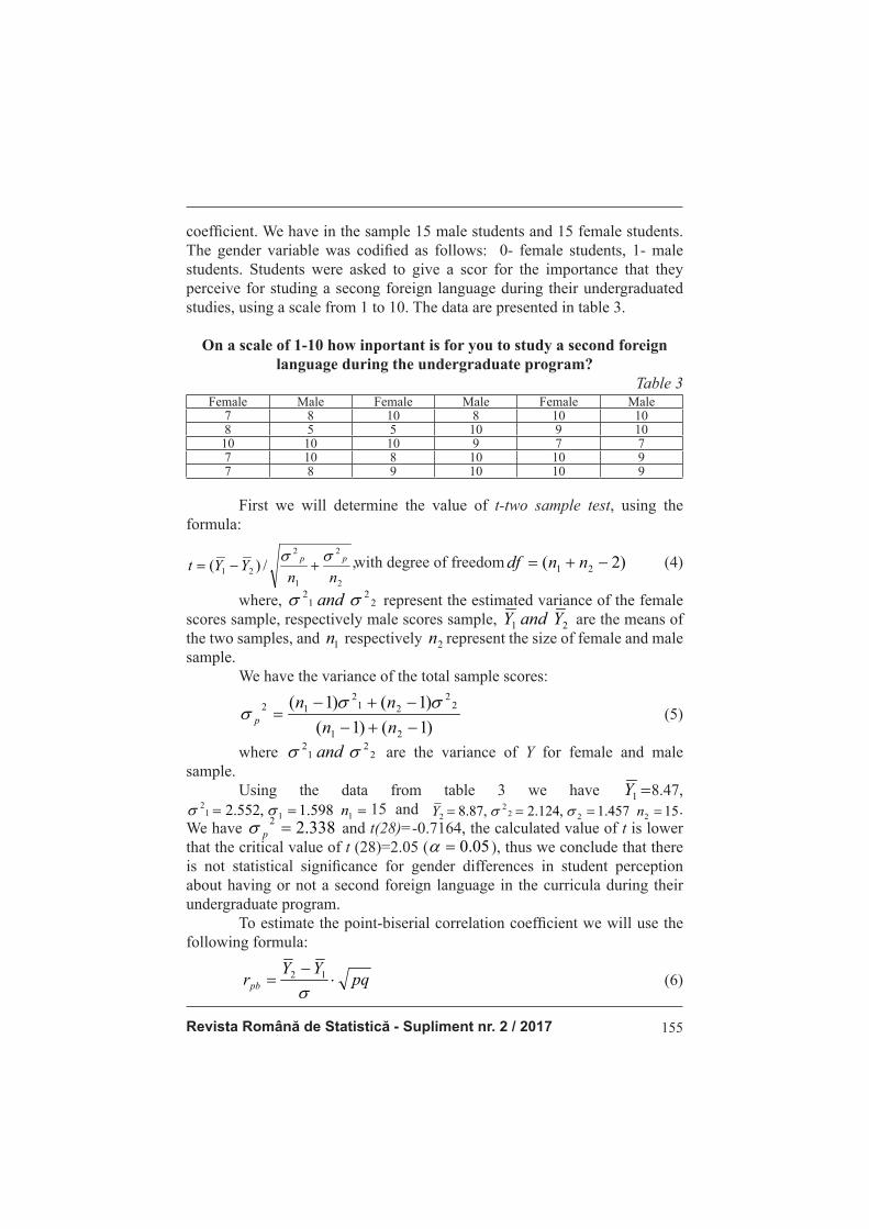
On a scale of 1-10 how inportant is for you to study a second foreign
language during the undergraduate program?
Table 3Female Male Female Male Female Male
7 8 10 8 10 108 5 5 10 9 10
10 10 10 9 7 77 10 8 10 10 97 8 9 10 10 9
First we will determine the value of t-two sample test, using the
formula:
2
2
1
2
21 /)(nn
YYtpp σσ
+−= ,with degree of freedom /��+�)�������������)�� ; 9 ' ��� ���� ��������������������������������������9!;���
�
�
�
%'(#'
�
(4)
where, 22
12 σσ and represent the estimated variance of the female
scores sample, respectively male scores sample, 21 YandY are the means of
the two samples, and 1n respectively 2n represent the size of female and male
sample.
We have the variance of the total sample scores:
)1()1(
)1()1(
21
22
212
12
−+−
−+−=
nn
nnp
σσσ (5)
where 22
12 σσ and are the variance of Y for female and male
sample.
Using the data from table 3 we have 81 =Y 8.47,
15598.1,552.2 1112 === nσσ 15 and '%!%F#'�' !# �2F#2
���� �� �� #�
�
%'(#'
�
.
We have 338.22 =pσ and t(28)=-0.7164, the calculated value of t is lower
that the critical value of t (28)=2.05 (� 9 2;K #$%�9 $%#$�� ;����� ���������)����,�� �,������-����+���������
�
�
%'(#'
�
), thus we conclude that there
is not statistical signifi cance for gender differences in student perception
about having or not a second foreign language in the curricula during their
undergraduate program.
To estimate the point-biserial correlation coeffi cient we will use the
following formula:
�-
���� �
��
�' ��������������������������������������������������� (6)

Romanian Statistical Review - Supplement nr. 2 / 2017156
where 1Y and 2Y have the above presented meaning, σ is the standard deviation of the whole sample, p and q represents the proportion of female and male students in the total sample.
For our study we have �����������)��/��+������ %#$%#$%'(#'
!F#22F#2��
���� K$#'& ����,������������ ��������+������������+��
�� �� �+���/��+� �+��5�� �����6�������)���9����$����';�� �� ������������+��� ��������+���������� ��)�
=0.132, a positive
association that suggest the fact that with the “increase” of gender (from 0 to 1), increase also the score for having a second foreign language in the undergraduate curricula. However, the difference is not statistical signifi cant.
The relationship between the point-biserial coeffi cient and the
estimated t statistics derived from the two-sample t test is given by the
relations (Chen and Popovich, 2002, p.28):
#; 9
'
JJ
'
' ���
�'����
� ��
��
��
�������
�� ��������������������������������������������������� (7)
Indeed we have 3�)��)�/�� +���� F'#$ '%'%;'& #$9'
'& #$
' '
����
�����
���
��
��� /+� +� �+�� ������ ���
;F'(!#$9�
�
which the value is of || t . And �#�G�)�
'
;F'(!#$9; '%'%9
;F'(!#$9
; 9 ����
��� ���
�K$#$'F==(�/+� +�����+�����������
�
which is the value of K$#$'F==(�/+� +�����+����������� �� #�
�
.
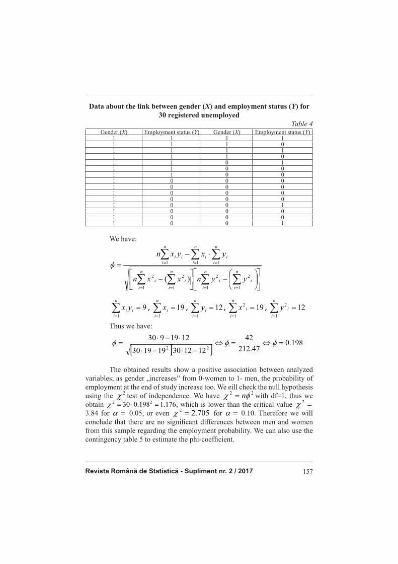
Phi coeffi cient (φ ) is another special case of Pearson correlation used
when both analyzed variables are naturally dichotomous. We will analyze in
this part of paper the association between gender of an individual (X) and his/
her employment status (employed/unemployed, Y), at the end of the observed
period. From the dataset gathered from National Agency of Romania, above
presented, we extracted a random sample of 30 individuals, from which 11
women (3 employed at the end of period) and 19 men (9 employed at the end
of period). Data are presented in table 4 and were coded as follows: 1- male
subjects, 0- female subjects, 1- employed, 0- unemployed.
Revista Română de Statistică - Supliment nr. 2 / 2017 157
Data about the link between gender (X) and employment status (Y) for
30 registered unemployed
Table 4Gender (X) Employment status (Y) Gender (X) Employment status (Y)
1 1 1 11 1 1 01 1 1 11 1 1 01 1 0 11 1 0 01 1 0 01 0 0 01 0 0 01 0 0 01 0 0 01 0 0 11 0 0 01 0 0 01 0 0 1
We have:
−
−
⋅−=
∑∑∑ ∑
∑∑ ∑
=== =
== =
n
i
i
n
i
i
n
i
n
i
ii
n
i
i
n
i
n
i
iii
yynxxn
yxyxn
1
2
1
2
1 1
22
11 1
)(
φ
='
���
�
�
�
� �� �� '='
���
�
�
�� �� ' '
���
�
�
�� �� '='
���
�
�
�� �� ' '
���
�
�
�� �
� Thus we have:
�
� �� �'=2#$
!F# '
!
' ' &$'='=&$
' '==&$
����
����
���� ��� �
�
�� ��
� �
�
�����
�
�
The obtained results show a positive association between analyzed variables; as gender „increases” from 0-women to 1- men, the probability of employment at the end of study increase too. We eill check the null hypothesis using the 2χ test of independence. We have 22 φχ n= with df=1, thus we obtain )�K'���+���/���-����� 'F(#''=2#$&$ ���� ��/+� +������/����+����+�� ���� ��������� 2!
�� ��
�
��
�
, which is lower than the critical value 32 =χ 3.84 for .0=α 0.05, or even 705.22 =χ for 0=α 0.10. Therefore we will conclude that there are no signifi cant differences between men and women
from this sample regarding the employment probability. We can also use the
contingency table 5 to estimate the phi-coeffi cient.
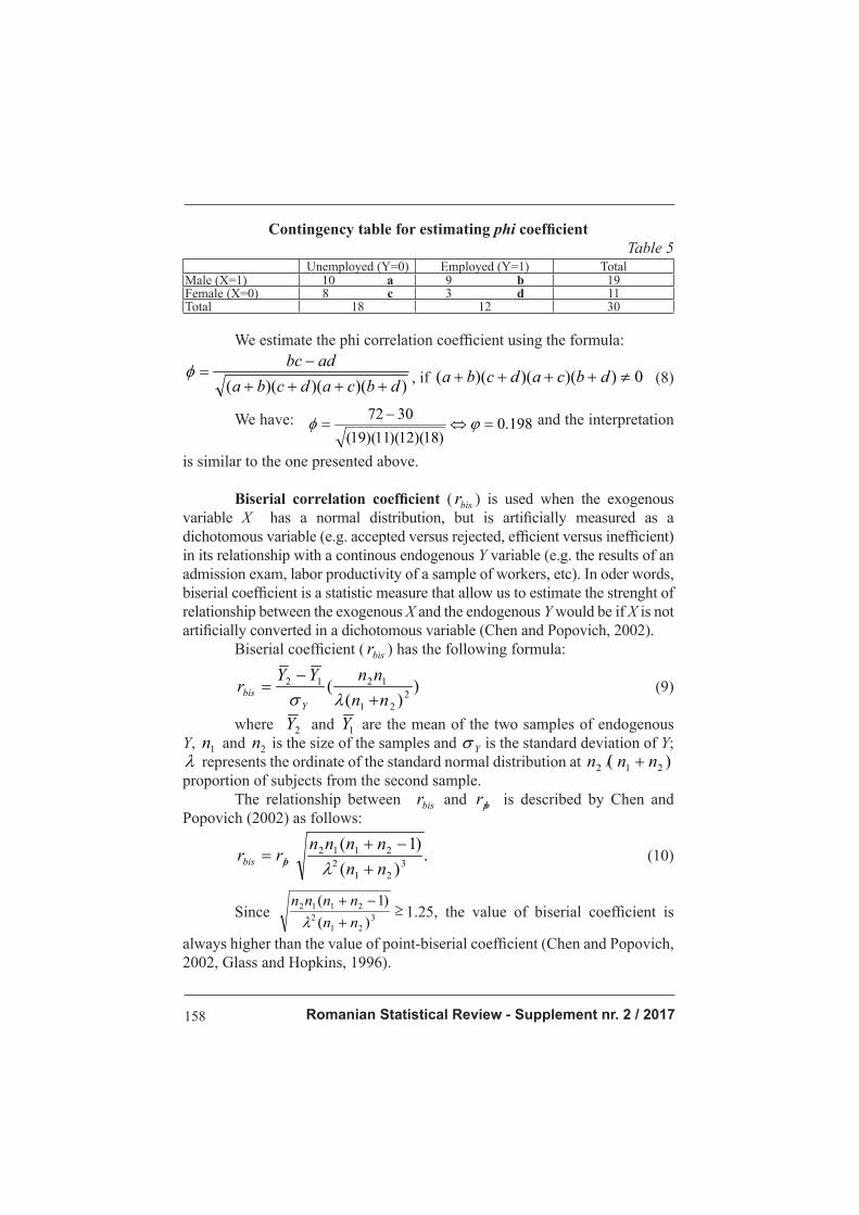
Romanian Statistical Review - Supplement nr. 2 / 2017158
Contingency table for estimating phi coeffi cient
Table 5Unemployed (Y=0) Employed (Y=1) Total
Male (X=1) 10 a 9 b 19Female (X=0) 8 c 3 d 11Total 18 12 30
We estimate the phi correlation coeffi cient using the formula:
;;9;9;99 �� �� ��
���
����
��� �����
&$F �
, if ;
������ $;;9;9;99 ����� �� �� �� �����������������������������������������92;�
�
�
(8)
We have: H�� +���1� '=2#$;'2;9' ;9'';9'=9
&$F ��
�� �� � � ��)� �+�� �����,��������� ��� ������� ��� �+�� ���� and the interpretation
is similar to the one presented above.
Biserial correlation coeffi cient ( bisr ) is used when the exogenous
variable X has a normal distribution, but is artifi cially measured as a
dichotomous variable (e.g. accepted versus rejected, effi cient versus ineffi cient)
in its relationship with a continous endogenous Y variable (e.g. the results of an
admission exam, labor productivity of a sample of workers, etc). In oder words,
biserial coeffi cient is a statistic measure that allow us to estimate the strenght of
relationship between the exogenous X and the endogenous Y would be if X is not
artifi cially converted in a dichotomous variable (Chen and Popovich, 2002).
Biserial coeffi cient ( bisr ) has the following formula:
))(
(2
21
1212
nn
nnYYr
Y
bis +
−=
λσ (9)
where 2Y and 1Y are the mean of the two samples of endogenous
Y, 1n and 2n is the size of the samples and Yσ is the standard deviation of Y;
λ represents the ordinate of the standard normal distribution at )/( 212 nnn +proportion of subjects from the second sample.
The relationship between bisr and pbr is described by Chen and
Popovich (2002) as follows:
.)(
)1(3
21
2
2112
nn
nnnnrr pbbis +
−+=
λ (10)
Since .1)(
)1(3
21
2
2112 ≥+
−+
nn
nnnn
λ1.25, the value of biserial coeffi cient is
always higher than the value of point-biserial coeffi cient (Chen and Popovich,
2002, Glass and Hopkins, 1996).

Revista Română de Statistică - Supliment nr. 2 / 2017 159
Tetrachoric coeffi cient, noted with tetr is used for estimating the relationship between two countinous variables X and Y, both of them artifi cially
transformed in dihotomous variables. In order to highlights how to use this
coeefi cient of correlation, we will estimate the intensity of relationship between
education (exogenous variable X) and unemployment duration (endogenous
variable Y) for a random sample of 30 unemployed subjects. The variable
education is expressed in number of study for each unemployed person. The
sample is extracted from the initial dataset of 2376253 unemployment spells.
The data are presented in table 6.
Data about the association between unemployment duration (days) and
education (years of study) for 30 registered unemployed persons
Table 6Nr. crt
Unemployment duration (days)
Education (years)
Nr.crt.
Unemployment duration (days)
Education (years)
Nr.crt
Unemployment duration (days)
Education (years)
1 365 8 11 260 8 21 140 132 20 16 12 300 10 22 156 123 270 10 13 240 12 23 30 164 190 12 14 190 14 24 32 165 60 18 15 195 16 25 67 186 360 4 16 40 18 26 12 207 90 6 17 10 16 27 300 98 180 12 18 185 12 28 23 129 181 12 19 360 4 29 180 13
10 182 14 20 365 12 30 181 14
As we can notice from table 6, both variables are continonus. We will
transform the education variable in a dichomotous variable with two categories,
„low-educated” (education<=12 years) and „good-educated” (education>12
years) and the duration of unemployment variable in a dichomotous variable
too, with the categories „short-term unemployment” (duration<180 days)
and „long-term unemployment” (duration>=180 zile). The initial data are
rearanged in table 7.
Contingency table for the link between unemployment duration and
education, 30 subjects sample
Table 7
Long-term
unemployment (Y=0)
Short-term
unemployment (Y=1)Total
Good-educated (X=1) 5 a 9 b 14 (a+b)Poor-educated (X=0) 13 c 3 d 16 (c+d)Total 18 (a+c) 12 (b+d) 30 (a+b+c+d)

Romanian Statistical Review - Supplement nr. 2 / 2017160
Tetrachoric coeffi cient is estimated as follows (Chen and Popovich,
2002, p.38):
�
���
��
�����
�� ���������������������������������������������������, (11)
where n is the size of sample, Xλ is the ordinate of the standardized
normal distribution at (a+b)/(a+b+c+d) proportion of subjects with X=1, Yλis the ordinate of the standardized normal distribution at (b+d)/(a+b+c+d)
proportion of subjects with Y=1.
Therefore we have: �+�������� /�� +���1� ($F#$
&$N&$
'
&$
'!
'%''F
�
�
����� #� �+��� ������ ��� ����� +��� � ����� �����
�
S���� S���+�
���,������������
��)�� S���+�
���,������������
$$$� &#$$� '� '(#F$� �
$$'� $#2$� '� '%#=$� �
$$ � F#!$� '� '=#($� �
$$&� %#'$� '� '(#%$� �
$$!� =#$$� '� 'F#2$� �
$$%� %#$$� '� 'F#!$� �
$$(� =#'$� '� 'F#F$� �
$$F� F#!$� '� 'F#&$� �
$$2� 2#&$� '� '%#'$� �
$$=� &'#($� '� 'F#&$� �
$'$� F#'$� '� '#'$� �
$''� &$#F$� '� #%$� �
$' � &'#'$� '� $#2$� �
$'&� &'#%$� '� #'$� �
$'!� &!# $� '� '#2$� �
$'%� =#!$� '� '=#F$� �
. This value of
tetrachoric coeffi cient suggests a positive and intense relationship between
education and unemployment duration. With the „increase” of X values, from
0 to 1 (from poor-educated to good-educated), the value of Y „increase” too,
from 0 to 1 (from long-term unemployment to short-term unemployment).
However, as Glass and Hopkins (1996) underline, the tetrachoric
coeffi cient is not a robust measure of correlation for smaller than 400
registration samples. Both biserial and tetrachoric coeffi cients are rarely used
in practice; their use and interpretation requires a special attention (Chen and
Popovich, 2002; Glass and Hopkins, 1996).
Eta coeffi cient of correlation, noted with η , is another special case
of Pearson coeffi cient used for estimate the intensity of association between
a multichotomous exogenous variable (X) with n distinct categories, and
an endogenous variable (Y) with intervals or ratio scores. Eta correlation
coeffi cient can be used for nonlinear relationship too. Eta coeffi cient is used
in the context of ANOVA analysis.
We will use eta coeffi cient to analyze if there are signifi cant statistical
difference between the dynamic of the ILO unemployment rate for of young
individuals aged in between 15 and 19 years (fi rst group), 20-24 years (second
group) and 25-29 years (third group), for the period 2000-2015. We use the
data offered by the National Statistical Institute, Tempo-Online database. The
unemployment rate of youth is coded as follows: 1 for 15-19 group, 2- for 20-
24 group and 3- for 25-29 group. The data are presented in table 8.
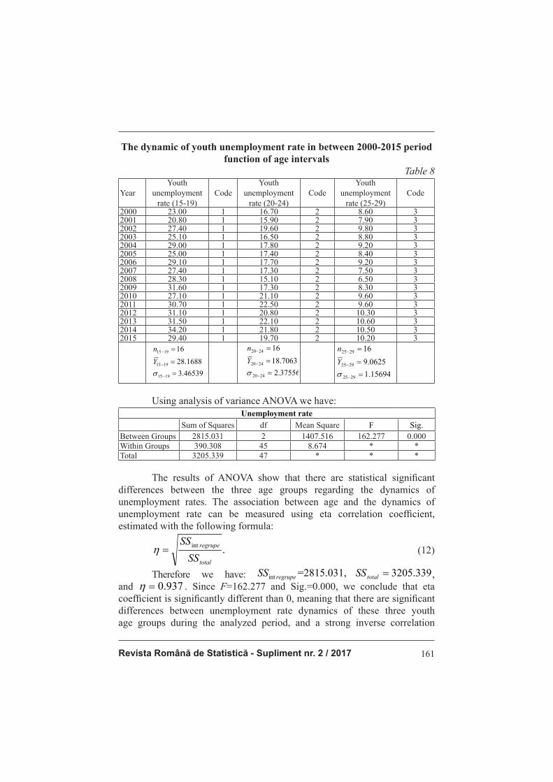
Revista Română de Statistică - Supliment nr. 2 / 2017 161
The dynamic of youth unemployment rate in between 2000-2015 period
function of age intervals
Table 8
YearYouth
unemployment rate (15-19)
CodeYouth
unemployment rate (20-24)
CodeYouth
unemployment rate (25-29)
Code
2000 23.00 1 16.70 2 8.60 32001 20.80 1 15.90 2 7.90 32002 27.40 1 19.60 2 9.80 32003 25.10 1 16.50 2 8.80 32004 29.00 1 17.80 2 9.20 32005 25.00 1 17.40 2 8.40 32006 29.10 1 17.70 2 9.20 32007 27.40 1 17.30 2 7.50 32008 28.30 1 15.10 2 6.50 32009 31.60 1 17.30 2 8.30 32010 27.10 1 21.10 2 9.60 32011 30.70 1 22.50 2 9.60 32012 31.10 1 20.80 2 10.30 32013 31.50 1 22.10 2 10.60 32014 34.20 1 21.80 2 10.50 32015 29.40 1 19.70 2 10.20 3�
&#!(%&=
2#'(22
'(
'='%
'='%
'='%
�
�
�
�
�
�
�
�
�
�
�
�
�
#&F%%(
'2#F$(&
'(
! $
! $
! $
�
�
�
�
�
�
�
�
��
�
�
#&F%%(
� �
'#'%(=!
=#$( %
'(
= %
= %
= %
�
�
�
�
�
�
�
�
�
��
�
Using analysis of variance ANOVA we have: Unemployment rate
Sum of Squares df Mean Square F Sig.Between Groups 2815.031 2 1407.516 162.277 0.000Within Groups 390.308 45 8.674 * *Total 3205.339 47 * * *
The results of ANOVA show that there are statistical signifi cant
differences between the three age groups regarding the dynamics of
unemployment rates. The association between age and the dynamics of
unemployment rate can be measured using eta correlation coeffi cient,
estimated with the following formula:
�������)�/��+��+�������/����������1�
#���
�����
�!���
&&
&&�� ��������������������������������������������������� (12)
Therefore we have: �+�������� /�� +���1� �!���&&��� K 2'%#$&'�� & $%#&&=������&& � ��)�
�
,
and 937.0=η . Since F=162.277 and Sig.=0.000, we conclude that eta
coeffi cient is signifi cantly different than 0, meaning that there are signifi cant
differences between unemployment rate dynamics of these three youth
age groups during the analyzed period, and a strong inverse correlation
Romanian Statistical Review - Supplement nr. 2 / 2017162
between age and unemployment rate of young people. If we use the mean values of unemployment rates instead of the codes 1, 2 and 3 (mean [15-19] unemployment rate= 28.1688 , mean [20-24] unemployment rate= 18.7063 and mean [25-34] unemployment rate=9.0625 ) and use the Pearson coeffi cient we get r= - 0,937, we observe that 937.0|| =r , which is exactly
the value of eta coeffi cient.
4. Conclusions
Pearson correlation coeffi cient is widely used in statistic analysis to
estimate the relationship between different variables; however its subtle nuances
and versatile nature are not generally well-known and are insuffi ciently investigated
in the literature. The aim of this paper was to analyze this complex measure and
to present its problems and limitations. We focused on the most important factors
infl uencing the size, direction and interpretation of Pearson coeffi cient; using real
data we proved that the interpretation of the values of Pearson coeffi cient must be
presented with caution. For each case we must check if the interpretation is in line
with the particularities of data and the used model. In all basic statistics textbooks
we can fi nd a chapter or a section devoted to simple linear correlation and Pearson
coeffi cient. However, only a few cover the topic of factors infl uencing the size
and interpretation of r (mostly the lack of linearity). To our knowledge, there is no
approach of these aspects in the Romanian basic statistics textbooks.
We focused also on particular cases when one or both of the analyzed
variables are naturally dichotomous or artifi cially converted as dichotomous
variable. Using real data we illustrated how to use the point-biserial coeffi cient,
phi coeffi cient, tetrachoric coeffi cient and eta coeffi cient and how to interpret
the obtained results. The issues presented in this paper can be useful to
researchers, tutors who teach statistics and students.
References
1. Abrami, P.C., Cholmsky, P., and Gordon, R. (2001), Statistical analysis for the
social sciences: An Interactive Approach. Needham Heights, MA: Allyn & Bacon. 2. Bobko, P. (1995), Correlation and Regression: Principles and Applications for
Industrial Organizational Psycology and Management, New York: Mc.Graw-Hill. 3. Brase, C.H. and Brase, C.P. (1999), Understanding statistics: Concepts and
Methods (6th ed.), Boston: Houghton Miffl in.
4. Cahan, S. (1965), On the Interpretation of the Product Moment Correlation
Coeffi cient as a Measure. Unpublished manuscript. The Hebrew University,
School of Education, Jerusalem, Israel.
4. Carroll, J. B. (1961), „The nature of the data, or how to choose a correlation
coeffi cient” Psychometrika, 26, pp. 247–272.
5. Chen, P.Y. and Popovich, P.M. (2002), Correlation: Parametric and Nonparametric
Measures. Sage University Papers Series on Quantitative Applications in the Social
Sciences, 07-139, Thousand Oaks, CA: Sage.
Revista Română de Statistică - Supliment nr. 2 / 2017 163
6. Dănăcică, D. (2013), Cercetări privind impactul factorilor ce infl uenţează durata
șomajului şi probabilitatea (re)angajării în România, Editura Academiei Române, București.
7. Eisenbach, R and Falk, R. (1984), „Association between Two Variables Measured
as Proportion of Loss Reduction”, Teaching Statistics, 6(2), pp. 47-52 8. Falk, R. and Well, A.D. (1996), „Correlation as Probability of Common Descent”,
Multivariate Behavavioral Research 31(2), pp.219-238. 9. Falk, R. and Well A.D. (1997), “Many Faces of the Correlation Coeffi cient”,
Journal of Statistics Education, 5 (3), pp. 1-12. 10. Glass, G.V. and Hopkins, K.D. (1996), Statistical Methods in Psychology and
Education (3rd ed.). Needham Heights, M.A.: Allyn and Bacon. 11. Goodwin, L.D. and Leech, N.L. (2006), “Understanding Correlation: Factors
that Affect the Size of r, The Journal of Experimental Education, 74(3), pp. 251-266.
12. Hays, W.L. (1994), Statistics (5th ed.), Forth Worth, TX: Harcourt Brace College Publishers.
13. Yule, G. U. and Kendall, M. G., (1950), An Introduction to the Theory of Statistics,
14th ed., rev. and enl. New York: Hafner. 14. Kruskal W.H. (1990), “Some remarks on wild observation”, Technometrics, 2,
pp.1-2. 15. Neter, J., Wasserman, W. and Kutner, M.H. (1989), Applied Linear Regressin
Mdels, Homewood, IL:Richard D. Irwin, Inc. 16. Nunnally, J. C., and Bernstein, I. H. (1994), Psychometric Theory (3rd ed.), New
York: McGraw-Hill. 17. Orr, J., Sackett P.R. and Dubois C. (2006), “Outlier Detectin and Treatment in
Psychology: A Survey of Researcher Beliefs and an Empirical Illustration”,
Personnel Psychology, Vol. 44, Issue 3, pp.473-486. 18. Ozer, D.J. (1985), “Correlation and the Coeffi cient of Determination”,
Psychological Bulletin, 97, pp.307-315. 19. Pearson, K. (1895), „Notes on the History of Correlation”, Biometrika, 13,
pp.25-45. 20. Pedhazur, E. J. (1973), Multiple Regression in Behavioral Research. New York:
Holt, Rinehart & Winston. 21. Rinaman, W.C. (1993), Foundation of Probability and Statistics, Fort Worth:
Saunders College Pub. 22. Rodgers,, J.L. and Nicewander, W.A. (1988), “Thirteen Ways to Look at the
Correlation Coeffi cient”, The American Statisticians, 42(1), pp.59-66. 23. Rovine, M. J., and von Eye, A. (1997), „A 14th Way to Look at a Correlation
Coeffi cient: Correlation as the Proportion of Matches”, The American Statistician, 51, pp. 42–46.
24. Stanton, J.M. (2001), “Galton, Pearson and the Peas: A Brief History of Linear
Regression for Statistics Instructors”, Journal of Statistics Education, 9 (3),
available at http://ww2.amstat.org/publications/jse/v9n3/stanton.html.