methods and techniques of complex system science
TRANSCRIPT
8/6/2019 Methods and Techniques of complex system science
http://slidepdf.com/reader/full/methods-and-techniques-of-complex-system-science 1/96
a r X i v : n l i n / 0 3
0 7 0 1 5 v 4 [ n l i n . A O
] 2 4 M a r 2 0 0 6
Chapter 1
METHODS AND TECHNIQUES OF COMPLEXSYSTEMS SCIENCE: AN OVERVIEW
Cosma Rohilla ShaliziCenter for the Study of Complex Systems, University of Michigan, Ann Arbor, MI 48109 USA
Abstract In this chapter, I review the main methods and techniques of complexsystems science. As a first step, I distinguish among the broad patternswhich recur across complex systems, the topics complex systems sciencecommonly studies, the tools employed, and the foundational science of complex systems. The focus of this chapter is overwhelmingly on thethird heading, that of tools. These in turn divide, roughly, into toolsfor analyzing data, tools for constructing and evaluating models, and
tools for measuring complexity. I discuss the principles of statisticallearning and model selection; time series analysis; cellular automata;agent-based models; the evaluation of complex-systems models; infor-mation theory; and ways of measuring complexity. Throughout, I giveonly rough outlines of techniques, so that readers, confronted with newproblems, will have a sense of which ones might be suitable, and whichones definitely are not.
1. Introduction
A complex system, roughly speaking, is one with many parts, whosebehaviors are both highly variable and strongly dependent on the be-havior of the other parts. Clearly, this includes a large fraction of the
universe! Nonetheless, it is not vacuously all-embracing: it excludes bothsystems whose parts just cannot do very much, and those whose partsare really independent of each other. “Complex systems science” is thefield whose ambition is to understand complex systems. Of course, this isa broad endeavor, overlapping with many even larger, better-establishedscientific fields. Having been asked by the editors to describe its meth-
8/6/2019 Methods and Techniques of complex system science
http://slidepdf.com/reader/full/methods-and-techniques-of-complex-system-science 2/96
2
Patterns
Topics Tools
Foundations
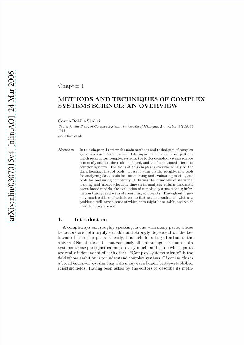
Figure 1.1. The quadrangle of complex systems. See text.
ods and techniques, I begin by explaining what I feel does not fall withinmy charge, as indicated by Figure 1.1.
At the top of Figure 1.1 I have put “patterns”. By this I mean more orless what people in software engineering do [1]: a pattern is a recurringtheme in the analysis of many different systems, a cross-systemic regu-larity. For instance: bacterial chemotaxis can be thought of as a way of resolving the tension between the exploitation of known resources, and
costly exploration for new, potentially more valuable, resources (Figure1.2). This same tension is present in a vast range of adaptive systems.Whether the exploration-exploitation trade-off arises among artificialagents, human decision-makers or colonial organisms, many of the issuesare the same as in chemotaxis, and solutions and methods of investiga-tion that apply in one case can profitably be tried in another [2, 3]. Thepattern “trade-off between exploitation and exploration” thus serves toorient us to broad features of novel situations. There are many othersuch patterns in complex systems science: “stability through hierarchi-cally structured interactions” [4], “positive feedback leading to highlyskewed outcomes” [5], “local inhibition and long-rate activation createspatial patterns” [6], and so forth.
At the bottom of the quadrangle is “foundations”, meaning attemptsto build a basic, mathematical science concerned with such topics asthe measurement of complexity [10], the nature of organization [11], therelationship between physical processes and information and computa-tion [12] and the origins of complexity in nature and its increase (ordecrease) over time. There is dispute whether such a science is possible,if so whether it would be profitable. I think it is both possible and use-
8/6/2019 Methods and Techniques of complex system science
http://slidepdf.com/reader/full/methods-and-techniques-of-complex-system-science 3/96
Overview of Methods and Techniques 3
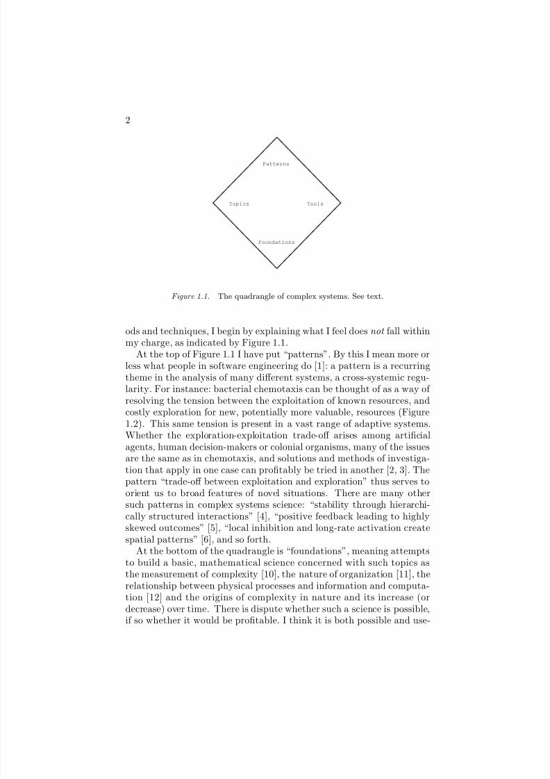
Figure 1.2. Bacterial chemotaxis. Should the bacterium (center) exploit thecurrently-available patch of food, or explore, in hopes of finding richer patches else-where (e.g. at right)? Many species solve this problem by performing a random walk(jagged line), tumbling randomly every so often. The frequency of tumbling increaseswhen the concentration of nutrients is high, making the bacterium take long steps inresource-poor regions, and persist in resource-rich ones [7–9].
ful, but most of what has been done in this area is very far from beingapplicable to biomedical research. Accordingly, I shall pass it over, withthe exception of a brief discussion of some work on measuring complexityand organization which is especially closely tied to data analysis.
“Topics” go in the left-hand corner. Here are what one might callthe “canonical complex systems”, the particular systems, natural, ar-tificial and fictional, which complex systems science has traditionallyand habitually sought to understand. Here we find networks (Wuchty,Ravasz and Barabasi, this volume), turbulence [13], physio-chemical pat-tern formation and biological morphogenesis [14, 15], genetic algorithms[16, 17], evolutionary dynamics [18, 19], spin glasses [20, 21], neuronalnetworks (see Part III, 4, this book), the immune system (see Part III,5, this book), social insects, ant-like robotic systems, the evolution of cooperation, evolutionary economics, etc.1 These topics all fall withinour initial definition of “complexity”, though whether they are studiedtogether because of deep connections, or because of historical accidentsand tradition, is a difficult question. In any event, this chapter will not describe the facts and particular models relevant to these topics.
Instead, this chapter is about the right-hand corner, “tools”. Some areprocedures for analyzing data, some are for constructing and evaluatingmodels, and some are for measuring the complexity of data or models.In this chapter I will restrict myself to methods which are generallyaccepted as valid (if not always widely applied), and seem promising for
8/6/2019 Methods and Techniques of complex system science
http://slidepdf.com/reader/full/methods-and-techniques-of-complex-system-science 4/96
4
biomedical research. These still demand a book, if not an encyclopedia,rather than a mere chapter! Accordingly, I will merely try to convey theessentials of the methods, with pointers to references for details. Thegoal is for you to have a sense of which methods would be good thingsto try on your problem, rather than to tell you everything you need toknow to implement them.
1.1 Outline of This Chapter
As mentioned above, the techniques of complex systems science can,for our purposes, be divided into three parts: those for analyzing data(perhaps without reference to a particular model), those for building
and understanding models (often without data), and those for measuringcomplexity as such. This chapter will examine them in that order.
The first part, on data, opens with the general ideas of statisticallearning and data mining (§1.2), namely developments in statisticsand machine learning theory that extend statistical methods beyondtheir traditional domain of low-dimensional, independent data. We thenturn to time series analysis (§1.3), where there are two importantstreams of work, inspired by statistics and nonlinear dynamics.
The second part, on modeling, considers the most important anddistinctive classes of models in complex systems. On the vital area of nonlinear dynamics, let the reader consult Socoloar (this volume).Cellular automata (
§1.4) allow us to represent spatial dynamics in a
way which is particularly suited to capturing strong local interactions,spatial heterogeneity, and large-scale aggregate patterns. Complemen-tary to cellular automata are agent-based models (§1.5), perhaps themost distinctive and most famous kind of model in complex systems sci-ence. A general section (1.6) on evaluating complex models, includ-ing analytical methods, various sorts of simulation, and testing, closesthis part of the chapter.
The third part of the chapter considers ways of measuring complexity.As a necessary preliminary, §1.7 introduces the concepts of informationtheory, with some remarks on its application to biological systems.Then §1.8 treats complexity measures, describing the main kindsof complexity measure, their relationships, and their applicability toempirical questions.
The chapter ends with a guide to further reading, organized by section.These emphasize readable and thorough introductions and surveys overmore advanced or historically important contributions.
8/6/2019 Methods and Techniques of complex system science
http://slidepdf.com/reader/full/methods-and-techniques-of-complex-system-science 5/96
Overview of Methods and Techniques 5
2. Statistical Learning and Data-Mining
Complex systems, we said, are those with many strongly interdepen-dent parts. Thanks to comparatively recent developments in statisticsand machine learning, it is now possible to infer reliable, predictive mod-els from data, even when the data concern thousands of strongly depen-dent variables. Such data mining is now a routine part of many indus-tries, and is increasingly important in research. While not, of course, asubstitute for devising valid theoretical models, data mining can tell uswhat kinds of patterns are in the data, and so guide our model-building.
2.1 Prediction and Model Selection
The basic goal of any kind of data mining is prediction: some vari-ables, let us call them X , are our inputs. The output is another variableor variables Y . We wish to use X to predict Y , or, more exactly, wewish to build a machine which will do the prediction for us: we will putin X at one end, and get a prediction for Y out at the other.2
“Prediction” here covers a lot of ground. If Y are simply other vari-ables like X , we sometimes call the problem regression. If they areX at another time, we have forecasting, or prediction in a strict senseof the word. If Y indicates membership in some set of discrete cate-gories, we have classification. Similarly, our predictions for Y can takethe form of distinct, particular values (point predictions), of ranges
or intervals we believe Y will fall into, or of entire probability distri-butions for Y , i.e., guesses as to the conditional distribution Pr(Y |X ).One can get a point prediction from a distribution by finding its meanor mode, so distribution predictions are in a sense more complete, butthey are also more computationally expensive to make, and harder tomake successfully.
Whatever kind of prediction problem we are attempting, and withwhatever kind of guesses we want our machine to make, we must be ableto say whether or not they are good guesses; in fact we must be able tosay just how much bad guesses cost us. That is, we need a loss functionfor predictions3. We suppose that our machine has a number of knobsand dials we can adjust, and we refer to these parameters, collectively,
as θ. The predictions we make, with inputs X and parameters θ, aref (X, θ), and the loss from the error in these predictions, when the actualoutputs are Y , is L(Y, f (X, θ)). Given particular values y and x, we have
the empirical loss L(y, f (x, θ)), or L(θ) for short4.Now, a natural impulse at this point is to twist the knobs to make
the loss small: that is, to select the θ which minimizes L(θ); let’s write
this θ = argminθ L(θ). This procedure is sometimes called empirical
8/6/2019 Methods and Techniques of complex system science
http://slidepdf.com/reader/full/methods-and-techniques-of-complex-system-science 6/96
6
risk minimization, or ERM. (Of course, doing that minimization canitself be a tricky nonlinear problem, but I will not cover optimizationmethods here.) The problem with ERM is that the θ we get from thisdata will almost surely not be the same as the one we’d get from thenext set of data. What we really care about, if we think it through, isnot the error on any particular set of data, but the error we can expect on new data, E [L(θ)]. The former, L(θ), is called the training or in-sample or empirical error; the latter, E [L(θ)], the generalization orout-of-sample or true error. The difference between in-sample andout-of-sample errors is due to sampling noise, the fact that our dataare not perfectly representative of the system we’re studying. There will
be quirks in our data which are just due to chance, but if we minimizeL blindly, if we try to reproduce every feature of the data, we will bemaking a machine which reproduces the random quirks, which do notgeneralize, along with the predictive features. Think of the empiricalerror L(θ) as the generalization error, E [L(θ)], plus a sampling fluctu-ation, ǫ. If we look at machines with low empirical errors, we will pickout ones with low true errors, which is good, but we will also pick outones with large negative sampling fluctuations, which is not good. Evenif the sampling noise ǫ is very small, θ can be very different from θmin.We have what optimization theory calls an ill-posed problem [22].
Having a higher-than-optimal generalization error because we paidtoo much attention to our data is called over-fitting. Just as we are
often better off if we tactfully ignore our friends’ and neighbors’ littlefaults, we want to ignore the unrepresentative blemishes of our sam-ple. Much of the theory of data mining is about avoiding over-fitting.Three of the commonest forms of tact it has developed are, in order of sophistication, cross-validation, regularization (or penalties) andcapacity control.
2.1.1 Validation. We would never over-fit if we knew howwell our machine’s predictions would generalize to new data. Since ourdata is never perfectly representative, we always have to estimate thegeneralization performance. The empirical error provides one estimate,but it’s biased towards saying that the machine will do well (since we
built it to do well on that data). If we had a second, independent set of data, we could evaluate our machine’s predictions on it, and that wouldgive us an unbiased estimate of its generalization. One way to do thisis to take our original data and divide it, at random, into two parts,the training set and the test set or validation set. We then use thetraining set to fit the machine, and evaluate its performance on the testset. (This is an instance of resampling our data, which is a useful trick
8/6/2019 Methods and Techniques of complex system science
http://slidepdf.com/reader/full/methods-and-techniques-of-complex-system-science 7/96
Overview of Methods and Techniques 7
in many contexts.) Because we’ve made sure the test set is independentof the training set, we get an unbiased estimate of the out-of-sampleperformance.
In cross-validation , we divide our data into random training andtest sets many different ways, fit a different machine for each trainingset, and compare their performances on their test sets, taking the onewith the best test-set performance. This re-introduces some bias —it could happen by chance that one test set reproduces the samplingquirks of its training set, favoring the model fit to the latter. But cross-validation generally reduces over-fitting, compared to simply minimizingthe empirical error; it makes more efficient use of the data, though it
cannot get rid of sampling noise altogether.
2.1.2 Regularization or Penalization. I said that the prob-lem of minimizing the error is ill-posed, meaning that small changes inthe errors can lead to big changes in the optimal parameters. A standardapproach to ill-posed problems in optimization theory is called regular-ization. Rather than trying to minimize L(θ) alone, we minimize
L(θ) + λd(θ) , (1.1)
where d(θ) is a regularizing or penalty function. Remember that
L(θ) = E [L(θ)] + ǫ, where ǫ is the sampling noise. If the penalty term
is well-designed, then the θ which minimizesE [L(θ)] + ǫ + λd(θ) (1.2)
will be close to the θ which minimizes E [L(θ)] — it will cancel out theeffects of favorable fluctuations. As we acquire more and more data, ǫ →0, so λ, too, goes to zero at an appropriate pace, the penalized solutionwill converge on the machine with the best possible generalization error.
How then should we design penalty functions? The more knobs anddials there are on our machine, the more opportunities we have to getinto mischief by matching chance quirks in the data. If one machinewith fifty knobs, and another fits the data just as well but has onlya single knob, we should (the story goes) chose the latter — becauseit’s less flexible, the fact that it does well is a good indication thatit will still do well in the future. There are thus many regularizationmethods which add a penalty proportional to the number of knobs, or,more formally, the number of parameters. These include the Akaikeinformation criterion or AIC [23] and the Bayesian information criterionor BIC [24, 25]. Other methods penalized the “roughness” of a model,i.e., some measure of how much the prediction shifts with a small change
8/6/2019 Methods and Techniques of complex system science
http://slidepdf.com/reader/full/methods-and-techniques-of-complex-system-science 8/96
8
Loss
Complexity
GeneralizationEmpirical
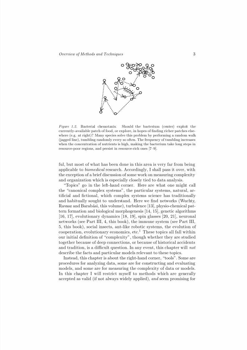
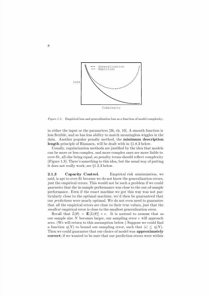
Figure 1.3. Empirical loss and generalization loss as a function of model complexity.
in either the input or the parameters [26, ch. 10]. A smooth function isless flexible, and so has less ability to match meaningless wiggles in thedata. Another p opular penalty method, the minimum descriptionlength principle of Rissanen, will be dealt with in §1.8.3 below.
Usually, regularization methods are justified by the idea that modelscan be more or less complex, and more complex ones are more liable to
over-fit, all else being equal, so penalty terms should reflect complexity(Figure 1.3). There’s something to this idea, but the usual way of puttingit does not really work; see §1.2.3 below.
2.1.3 Capacity Control. Empirical risk minimization, wesaid, is apt to over-fit because we do not know the generalization errors, just the empirical errors. This would not be such a problem if we couldguarantee that the in-sample performance was close to the out-of-sampleperformance. Even if the exact machine we got this way was not par-ticularly close to the optimal machine, we’d then be guaranteed thatour predictions were nearly optimal. We do not even need to guaranteethat all the empirical errors are close to their true values, just that thesmallest empirical error is close to the smallest generalization error.
Recall that L(θ) = E [L(θ)] + ǫ. It is natural to assume that asour sample size N becomes larger, our sampling error ǫ will approachzero. (We will return to this assumption below.) Suppose we could finda function η(N ) to bound our sampling error, such that |ǫ| ≤ η(N ).Then we could guarantee that our choice of model was approximatelycorrect; if we wanted to be sure that our prediction errors were within
8/6/2019 Methods and Techniques of complex system science
http://slidepdf.com/reader/full/methods-and-techniques-of-complex-system-science 9/96
Overview of Methods and Techniques 9
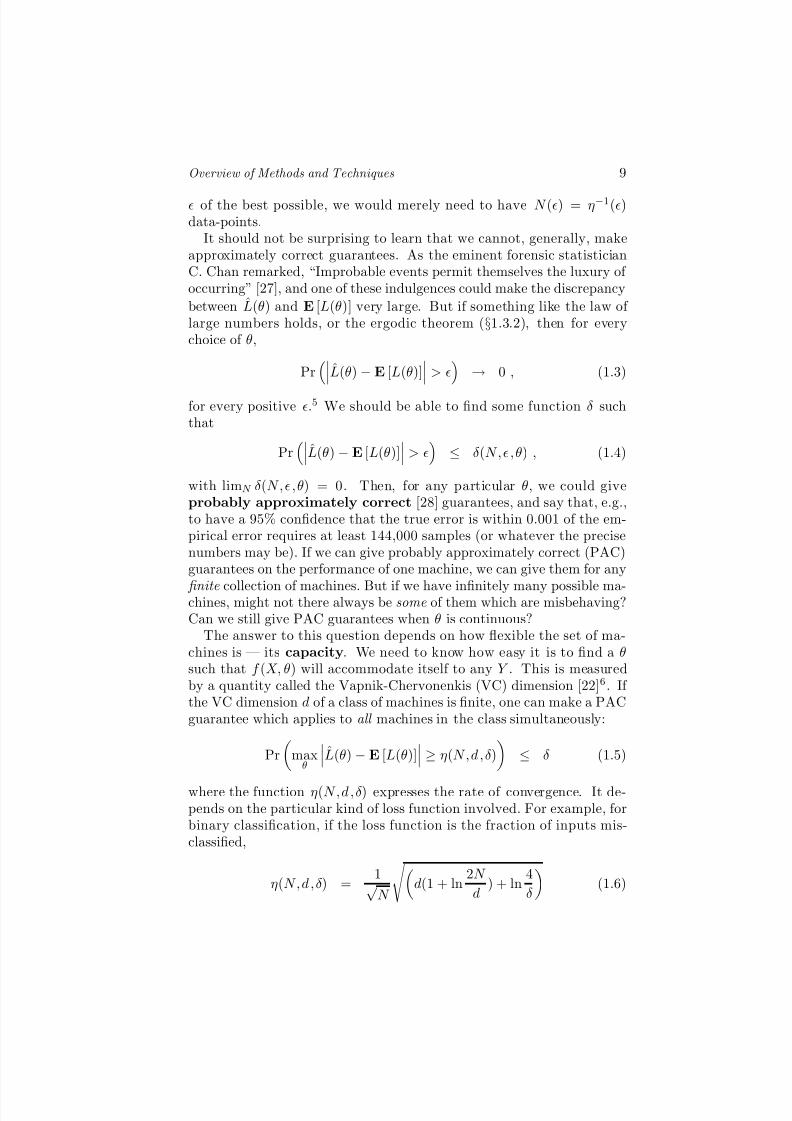
ǫ of the best possible, we would merely need to have N (ǫ) = η−1(ǫ)data-points.
It should not be surprising to learn that we cannot, generally, makeapproximately correct guarantees. As the eminent forensic statisticianC. Chan remarked, “Improbable events permit themselves the luxury of occurring” [27], and one of these indulgences could make the discrepancy
between L(θ) and E [L(θ)] very large. But if something like the law of large numbers holds, or the ergodic theorem (§1.3.2), then for everychoice of θ,
Pr L(θ) − E [L(θ)] > ǫ → 0 , (1.3)
for every positive ǫ.5 We should be able to find some function δ suchthat
PrL(θ) − E [L(θ)]
> ǫ
≤ δ(N,ǫ ,θ) , (1.4)
with limN δ(N,ǫ ,θ) = 0. Then, for any particular θ, we could giveprobably approximately correct [28] guarantees, and say that, e.g.,to have a 95% confidence that the true error is within 0.001 of the em-pirical error requires at least 144,000 samples (or whatever the precisenumbers may be). If we can give probably approximately correct (PAC)guarantees on the performance of one machine, we can give them for any
finite collection of machines. But if we have infinitely many possible ma-chines, might not there always be some of them which are misbehaving?Can we still give PAC guarantees when θ is continuous?
The answer to this question depends on how flexible the set of ma-chines is — its capacity. We need to know how easy it is to find a θsuch that f (X, θ) will accommodate itself to any Y . This is measuredby a quantity called the Vapnik-Chervonenkis (VC) dimension [22]6. If the VC dimension d of a class of machines is finite, one can make a PACguarantee which applies to all machines in the class simultaneously:
Pr
maxθ
L(θ) − E [L(θ)]
≥ η(N,d,δ)
≤ δ (1.5)
where the function η(N,d,δ) expresses the rate of convergence. It de-pends on the particular kind of loss function involved. For example, forbinary classification, if the loss function is the fraction of inputs mis-classified,
η(N,d,δ) =1√N
d(1 + ln
2N
d) + ln
4
δ
(1.6)
8/6/2019 Methods and Techniques of complex system science
http://slidepdf.com/reader/full/methods-and-techniques-of-complex-system-science 10/96
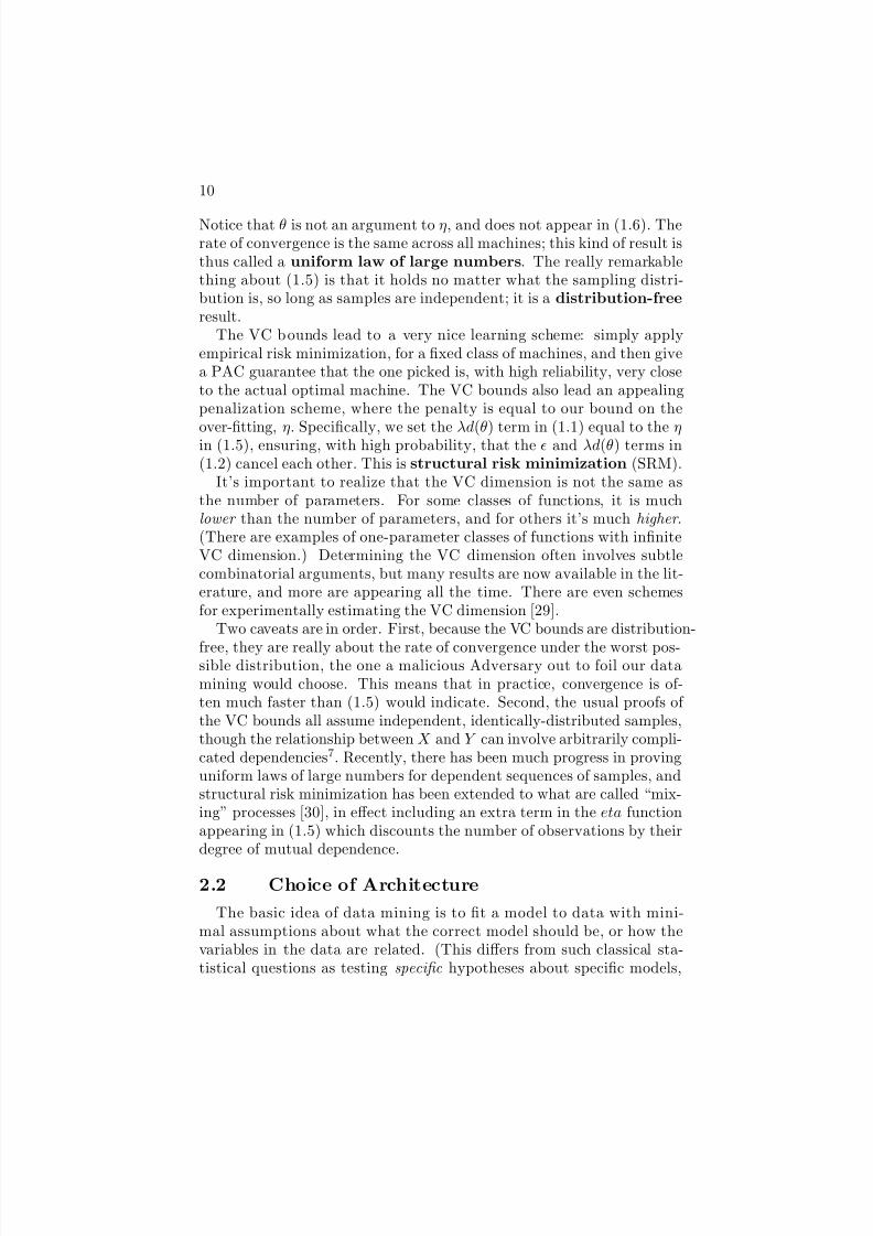
10
Notice that θ is not an argument to η, and does not appear in (1.6). Therate of convergence is the same across all machines; this kind of result isthus called a uniform law of large numbers. The really remarkablething about (1.5) is that it holds no matter what the sampling distri-bution is, so long as samples are independent; it is a distribution-freeresult.
The VC b ounds lead to a very nice learning scheme: simply applyempirical risk minimization, for a fixed class of machines, and then givea PAC guarantee that the one picked is, with high reliability, very closeto the actual optimal machine. The VC bounds also lead an appealingpenalization scheme, where the penalty is equal to our bound on the
over-fitting, η. Specifically, we set the λd(θ) term in (1.1) equal to the ηin (1.5), ensuring, with high probability, that the ǫ and λd(θ) terms in(1.2) cancel each other. This is structural risk minimization (SRM).
It’s important to realize that the VC dimension is not the same asthe number of parameters. For some classes of functions, it is muchlower than the number of parameters, and for others it’s much higher .(There are examples of one-parameter classes of functions with infiniteVC dimension.) Determining the VC dimension often involves subtlecombinatorial arguments, but many results are now available in the lit-erature, and more are appearing all the time. There are even schemesfor experimentally estimating the VC dimension [29].
Two caveats are in order. First, because the VC bounds are distribution-
free, they are really about the rate of convergence under the worst pos-sible distribution, the one a malicious Adversary out to foil our datamining would choose. This means that in practice, convergence is of-ten much faster than (1.5) would indicate. Second, the usual proofs of the VC bounds all assume independent, identically-distributed samples,though the relationship between X and Y can involve arbitrarily compli-cated dependencies7. Recently, there has been much progress in provinguniform laws of large numbers for dependent sequences of samples, andstructural risk minimization has been extended to what are called “mix-ing” processes [30], in effect including an extra term in the eta functionappearing in (1.5) which discounts the number of observations by theirdegree of mutual dependence.
2.2 Choice of Architecture
The basic idea of data mining is to fit a model to data with mini-mal assumptions about what the correct model should be, or how thevariables in the data are related. (This differs from such classical sta-tistical questions as testing specific hypotheses about specific models,

8/6/2019 Methods and Techniques of complex system science
http://slidepdf.com/reader/full/methods-and-techniques-of-complex-system-science 11/96
Overview of Methods and Techniques 11
such as the presence of interactions between certain variables.) This isfacilitated by the development of extremely flexible classes of models,which are sometimes, misleadingly, called non-parametric; a bettername would be megaparametric. The idea behind megaparametricmodels is that they should be capable of approximating any function, atleast any well-behaved function, to any desired accuracy, given enoughcapacity.
The polynomials are a familiar example of a class of functions whichcan perform such universal approximation. Given any smooth functionf , we can represent it by taking the Taylor series around our favoritepoint x0. Truncating that series gives an approximation to f :
f (x) = f (x0) +∞k=1
(x − x0)k
k!dkf dxk
x0
(1.7)
≈ f (x0) +nk=1
(x − x0)k
k!
dkf
dxk
x0
(1.8)
=nk=0
ak(x − x0)k
k!(1.9)
In fact, if f is an nth order polynomial, the truncated series is exact, notan approximation.
To see why this is not a reason to use only polynomial models, think
about what would happen if f (x) = sin x. We would need an infiniteorder polynomial to completely represent f , and the generalization prop-erties of finite-order approximations would generally be lousy: for onething, f is bounded between -1 and 1 everywhere, but any finite-orderpolynomial will start to zoom off to ∞ or −∞ outside some range. Of course, this f would be really easy to approximate as a superposition of sines and cosines, which is another class of functions which is capableof universal approximation (better known, perhaps, as Fourier analy-sis). What one wants, naturally, is to chose a model class which gives agood approximation of the function at hand, at low order . We want loworder functions, both because computational demands rise with modelorder, and because higher order models are more prone to over-fitting
(VC dimension generally rises with model order).To adequately describe all of the common model classes, or model
architectures, used in the data mining literature would require anotherchapter. ([31] and [32] are good for this.) Instead, I will merely name afew.
Splines are piecewise polynomials, good for regression on boundeddomains; there is a very elegant theory for their estimation [33].
8/6/2019 Methods and Techniques of complex system science
http://slidepdf.com/reader/full/methods-and-techniques-of-complex-system-science 12/96
12
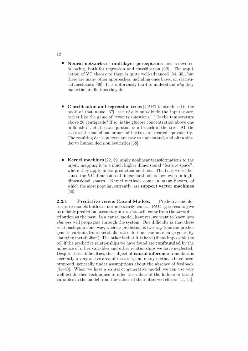
Neural networks or multilayer perceptrons have a devotedfollowing, both for regression and classification [32]. The appli-cation of VC theory to them is quite well-advanced [34, 35], butthere are many other approaches, including ones based on statisti-cal mechanics [36]. It is notoriously hard to understand why theymake the predictions they do.
Classification and regression trees (CART), introduced in thebook of that name [37], recursively sub-divide the input space,rather like the game of “twenty questions” (“Is the temperature
above 20 centigrade? If so, is the glucose concentration above onemillimole?”, etc.); each question is a branch of the tree. All thecases at the end of one branch of the tree are treated equivalently.The resulting decision trees are easy to understand, and often sim-ilar to human decision heuristics [38].
Kernel machines [22, 39] apply nonlinear transformations to theinput, mapping it to a much higher dimensional “feature space”,where they apply linear prediction methods. The trick works be-cause the VC dimension of linear methods is low, even in high-dimensional spaces. Kernel methods come in many flavors, of
which the most popular, currently, are support vector machines[40].
2.2.1 Predictive versus Causal Models. Predictive and de-scriptive models both are not necessarily causal. PAC-type results giveus reliable prediction, assuming future data will come from the same dis-tribution as the past. In a causal model, however, we want to know howchanges will propagate through the system. One difficulty is that theserelationships are one-way, whereas prediction is two-way (one can predictgenetic variants from metabolic rates, but one cannot change genes bychanging metabolism). The other is that it is hard (if not impossible) totell if the predictive relationships we have found are confounded by theinfluence of other variables and other relationships we have neglected.Despite these difficulties, the subject of causal inference from data iscurrently a very active area of research, and many methods have beenproposed, generally under assumptions about the absence of feedback[41–43]. When we have a causal or generative model, we can use verywell-established techniques to infer the values of the hidden or latentvariables in the model from the values of their observed effects [41, 44].
8/6/2019 Methods and Techniques of complex system science
http://slidepdf.com/reader/full/methods-and-techniques-of-complex-system-science 13/96
Overview of Methods and Techniques 13
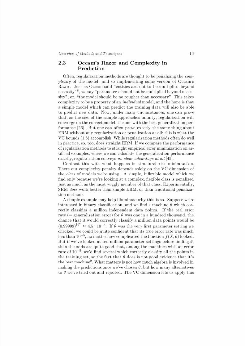
2.3 Occam’s Razor and Complexity inPrediction
Often, regularization methods are thought to be penalizing the com-plexity of the model, and so implementing some version of Occam’sRazor. Just as Occam said “entities are not to be multiplied beyondnecessity”8, we say “parameters should not be multiplied beyond neces-sity”, or, “the model should be no rougher than necessary”. This takescomplexity to be a property of an individual model, and the hope is thata simple model which can predict the training data will also be ableto predict new data. Now, under many circumstances, one can provethat, as the size of the sample approaches infinity, regularization will
converge on the correct model, the one with the best generalization per-formance [26]. But one can often prove exactly the same thing aboutERM without any regularization or penalization at all; this is what theVC bounds (1.5) accomplish. While regularization methods often do wellin practice, so, too, does straight ERM. If we compare the performanceof regularization methods to straight empirical error minimization on ar-tificial examples, where we can calculate the generalization performanceexactly, regularization conveys no clear advantage at all [45].
Contrast this with what happens in structural risk minimization.There our complexity penalty depends solely on the VC dimension of the class of models we’re using. A simple, inflexible model which wefind only because we’re looking at a complex, flexible class is penalized just as much as the most wiggly member of that class. Experimentally,SRM does work better than simple ERM, or than traditional penaliza-tion methods.
A simple example may help illuminate why this is so. Suppose we’reinterested in binary classification, and we find a machine θ which cor-rectly classifies a million independent data points. If the real errorrate (= generalization error) for θ was one in a hundred thousand, thechance that it would correctly classify a million data points would be
(0.99999)106 ≈ 4.5 · 10−5. If θ was the very first parameter setting wechecked, we could be quite confident that its true error rate was muchless than 10−5, no matter how complicated the function f (X, θ) looked.
But if we’ve looked at ten million parameter settings before finding θ,then the odds are quite good that, among the machines with an errorrate of 10−5, we’d find several which correctly classify all the points inthe training set, so the fact that θ does is not good evidence that it’sthe best machine9. What matters is not how much algebra is involved inmaking the predictions once we’ve chosen θ, but how many alternativesto θ we’ve tried out and rejected. The VC dimension lets us apply this
8/6/2019 Methods and Techniques of complex system science
http://slidepdf.com/reader/full/methods-and-techniques-of-complex-system-science 14/96
14
kind of reasoning rigorously and without needing to know the details of the process by which we generate and evaluate models.
The upshot is that the kind of complexity which matters for learning,and so for Occam’s Razor, is the complexity of classes of models, notof individual models nor of the system being modeled. It is importantto keep this point in mind when we try to measure the complexity of systems (§1.8).
2.4 Relation of Complex Systems Science toStatistics
Complex systems scientists often regard the field of statistics as irrel-
evant to understanding such systems. This is understandable, since theexposure most scientists have to statistics (e.g., the “research methods”courses traditional in the life and social sciences) typically deal withsystems with only a few variables and with explicit assumptions of inde-pendence, or only very weak dependence. The kind of modern methodswe have just seen, amenable to large systems and strong dependence,are rarely taught in such courses, or even mentioned. Considering theshaky grasp many students have on even the basic principles of statisti-cal inference, this is perhaps wise. Still, it leads to even quite eminentresearchers in complexity making disparaging remarks about statistics(e.g., “statistical hypothesis testing, that substitute for thought”), whileactually re-inventing tools and concepts which have long been familiarto statisticians.
For their part, many statisticians tend to overlook the very existenceof complex systems science as a separate discipline. One may hope thatthe increasing interest from both fields on topics such as bioinformaticsand networks will lead to greater mutual appreciation.
3. Time Series Analysis
There are two main schools of time series analysis. The older one,which has a long pedigree in applied statistics [46], and is prevalentamong statisticians, social scientists (especially econometricians) andengineers. The younger school, developed essentially since the 1970s,
comes out of physics and nonlinear dynamics. The first views time seriesas samples from a stochastic process, and applies a mixture of traditionalstatistical tools and assumptions (linear regression, the properties of Gaussian distributions) and the analysis of the Fourier spectrum. Thesecond school views time series as distorted or noisy measurements of an underlying dynamical system, which it aims to reconstruct.
8/6/2019 Methods and Techniques of complex system science
http://slidepdf.com/reader/full/methods-and-techniques-of-complex-system-science 15/96
8/6/2019 Methods and Techniques of complex system science
http://slidepdf.com/reader/full/methods-and-techniques-of-complex-system-science 16/96
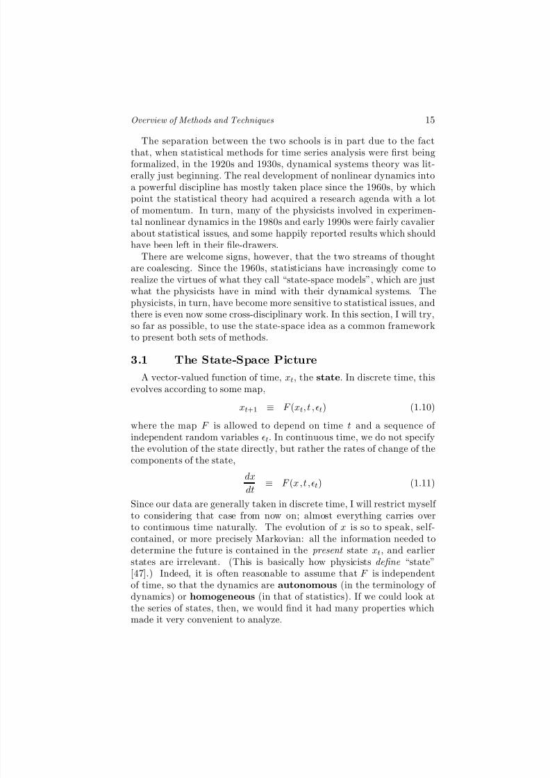
16
Sadly, however, we do not observe the state x; what we observe ormeasure is y, which is generally a noisy, nonlinear function of the state:yt = h(xt, ηt), where ηt is measurement noise. Whether y, too, hasthe convenient properties depends on h, and usually y is not convenient.Matters are made more complicated by the fact that we do not, in typicalcases, know the observation function h, nor the state-dynamics F , noreven, really, what space x lives in. The goal of time-series methods is tomake educated guess about all these things, so as to better predict andunderstand the evolution of temporal data.
In the ideal case, simply from a knowledge of y, we would be able toidentify the state space, the dynamics, and the observation function. As
a matter of pure mathematical possibility, this can be done for essen-tially arbitrary time-series [48, 49]. Nobody, however, knows how to dothis with complete generality in practice. Rather, one makes certain as-sumptions about, say, the state space, which are strong enough that theremaining details can be filled in using y. Then one checks the result foraccuracy and plausibility, i.e., for the kinds of errors which would resultfrom breaking those assumptions [50].
Subsequent parts of this section describe classes of such methods.First, however, I describe some of the general properties of time series,and general measurements which can be made upon them.
Notation. There is no completely uniform notation for time-series.
Since it will be convenient to refer to sequences of consecutive values.I will write all the measurements starting at s and ending at t as yts.Further, I will abbreviate the set of all measurements up to time t, yt−∞,as y−
t , and the future starting from t, y∞t+1, as y+
t .
3.2 General Properties of Time Series
One of the most commonly assumed properties of a time-series is sta-tionarity, which comes in two forms: strong or strict stationarity, andweak, wide-sense or second-order stationarity. Strong stationarity isthe property that the probability distribution of sequences of observa-tions does not change over time. That is,
Pr(Y t+ht ) = Pr(Y t+τ +ht+τ ) (1.12)
for all lengths of time h and all shifts forwards or backwards in timeτ . When a series is described as “stationary” without qualification, itdepends on context whether strong or weak stationarity is meant.
8/6/2019 Methods and Techniques of complex system science
http://slidepdf.com/reader/full/methods-and-techniques-of-complex-system-science 17/96
Overview of Methods and Techniques 17
Weak stationarity, on the other hand, is the property that the firstand second moments of the distribution do not change over time.
E [Y t] = E [Y t+τ ] (1.13)
E [Y tY t+h] = E [Y t+τ Y t+τ +h] (1.14)
If Y is a Gaussian process, then the two senses of stationarity are equiv-alent. Note that both sorts of stationarity are statements about the truedistribution, and so cannot be simply read off from measurements.
Strong stationarity implies a property called ergodicity, which ismuch more generally applicable. Roughly speaking, a series is ergodic if any sufficiently long sample is representative of the entire process. More
exactly, consider the time-average of a well-behaved function f of Y ,
f t2t1 ≡ 1
t2 − t1
t=t2t=t1
f (Y t) . (1.15)
This is generally a random quantity, since it depends on where the trajec-tory started at t1, and any random motion which may have taken placebetween then and t2. Its distribution generally depends on the precisevalues of t1 and t2. The series Y is ergodic if almost all time-averagesconverge eventually, i.e., if
limT →∞
f t+T t = f (1.16)
for some constant f independent of the starting time t, the startingpoint Y t, or the trajectory Y ∞t . Ergodic theorems specify conditionsunder which ergodicity holds; surprisingly, even completely deterministicdynamical systems can be ergodic.
Ergodicity is such an important property because it means that sta-tistical methods are very directly applicable. Simply by waiting longenough, one can obtain an estimate of any desired property which willbe closely representative of the future of the process. Statistical infer-ence is possible for non-ergodic processes, but it is considerably moredifficult, and often requires multiple time-series [51, 52].
One of the most basic means of studying a time series is to compute
the autocorrelation function (ACF), which measures the linear de-pendence between the values of the series at different points in time.This starts with the autocovariance function:
C (s, t) ≡ E [(ys − E [ys]) (yt − E [yt])] . (1.17)
(Statistical physicists, unlike anyone else, call this the “correlation func-tion”.) The autocorrelation itself is the autocovariance, normalized by
8/6/2019 Methods and Techniques of complex system science
http://slidepdf.com/reader/full/methods-and-techniques-of-complex-system-science 18/96
18
the variability of the series:
ρ(s, t) ≡ C (s, t) C (s, s)C (t, t)
(1.18)
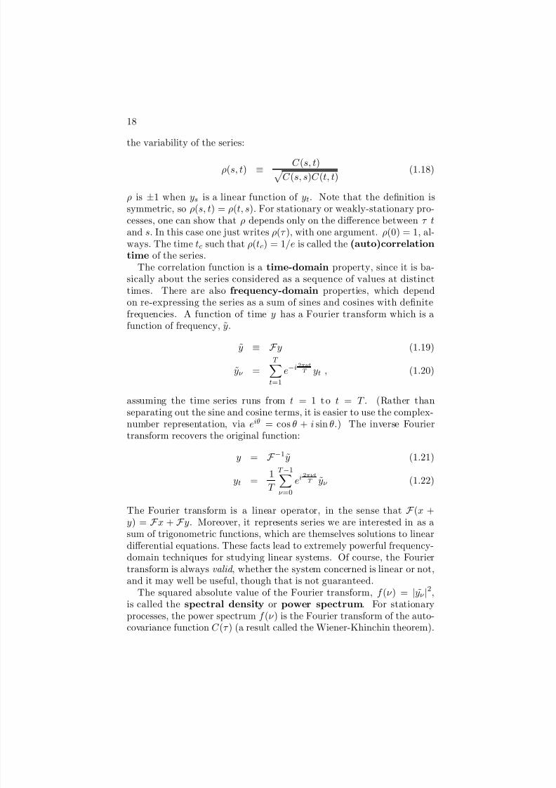
ρ is ±1 when ys is a linear function of yt. Note that the definition issymmetric, so ρ(s, t) = ρ(t, s). For stationary or weakly-stationary pro-cesses, one can show that ρ depends only on the difference between τ tand s. In this case one just writes ρ(τ ), with one argument. ρ(0) = 1, al-ways. The time tc such that ρ(tc) = 1/e is called the (auto)correlationtime of the series.
The correlation function is a time-domain property, since it is ba-
sically about the series considered as a sequence of values at distincttimes. There are also frequency-domain properties, which dependon re-expressing the series as a sum of sines and cosines with definitefrequencies. A function of time y has a Fourier transform which is afunction of frequency, y.
y ≡ F y (1.19)
yν =T t=1
e−i 2πνtT yt , (1.20)
assuming the time series runs from t = 1 t o t = T . (Rather than
separating out the sine and cosine terms, it is easier to use the complex-number representation, via eiθ = cos θ + i sin θ.) The inverse Fouriertransform recovers the original function:
y = F −1y (1.21)
yt =1
T
T −1ν =0
ei2πνtT yν (1.22)
The Fourier transform is a linear operator, in the sense that F (x +y) = F x + F y. Moreover, it represents series we are interested in as asum of trigonometric functions, which are themselves solutions to lineardifferential equations. These facts lead to extremely powerful frequency-domain techniques for studying linear systems. Of course, the Fouriertransform is always valid , whether the system concerned is linear or not,and it may well be useful, though that is not guaranteed.
The squared absolute value of the Fourier transform, f (ν ) = |yν |2,is called the spectral density or power spectrum. For stationaryprocesses, the power spectrum f (ν ) is the Fourier transform of the auto-covariance function C (τ ) (a result called the Wiener-Khinchin theorem).

8/6/2019 Methods and Techniques of complex system science
http://slidepdf.com/reader/full/methods-and-techniques-of-complex-system-science 19/96
Overview of Methods and Techniques 19
An important consequence is that a Gaussian process is completely spec-ified by its power spectrum. In particular, consider a sequence of inde-pendent Gaussian variables, each with variance σ2. Because they areperfectly uncorrelated, C (0) = σ2, and C (τ ) = 0 for any τ = 0. TheFourier transform of such a C (τ ) is just f (ν ) = σ2, independent of ν —every frequency has just as much p ower. Because white light has equalpower in every color of the spectrum, such a process is called whitenoise. Correlated processes, with uneven power spectra, are sometimescalled colored noise, and there is an elaborate terminology of red, pink,brown, etc. noises [53, ch. 3].
The easiest way to estimate the power spectrum is simply to take
the Fourier transform of the time series, using, e.g., the fast Fouriertransform algorithm [54]. Equivalently, one might calculate the autoco-variance and Fourier transform that. Either way, one has an estimateof the spectrum which is called the periodogram. It is unbiased, inthat the expected value of the periodogram at a given frequency is thetrue power at that frequency. Unfortunately, it is not consistent —the variance around the true value does not shrink as the series grows.The easiest way to overcome this is to apply any of several well-knownsmoothing functions to the periodogram, a procedure called windowing[55]. (Standard software packages will accomplish this automatically.)
The Fourier transform takes the original series and decomposes itinto a sum of sines and cosines. This is possible because any reasonable
function can be represented in this way. The trigonometric functions arethus a basis for the space of functions. There are many other possiblebases, and one can equally well perform the same kind of decompositionin any other basis. The trigonometric basis is particularly useful forstationary time series because the basis functions are themselves evenlyspread over all times [56, ch. 2]. Other bases, localized in time, are moreconvenient for non-stationary situations. The most well-known of thesealternate bases, currently, are wavelets [57], but there is, literally, nocounting the other possibilities.
3.3 The Traditional Statistical Approach
The traditional statistical approach to time series is to represent themthrough linear models of the kind familiar from applied statistics.
The most basic kind of model is that of a moving average, whichis especially appropriate if x is highly correlated up to some lag, say q,after which the ACF decays rapidly. The moving average model repre-sents x as the result of smoothing q + 1 independent random variables.

8/6/2019 Methods and Techniques of complex system science
http://slidepdf.com/reader/full/methods-and-techniques-of-complex-system-science 20/96
20
Specifically, the MA(q) model of a weakly stationary series is
yt = µ + wt +qk=1
θkwt−k (1.23)
where µ is the mean of y, the θi are constants and the wt are white noisevariables. q is called the order of the model. Note that there is nodirect dependence between successive values of y; they are all functionsof the white noise series w. Note also that yt and yt+q+1 are completelyindependent; after q time-steps, the effects of what happened at time tdisappear.
Another basic model is that of an autoregressive process, wherethe next value of y is a linear combination of the preceding values of y.Specifically, an AR( p) model is
yt = α + pk=1
φkyt−k + wt (1.24)
where φi are constants and α = µ(1− pk=1 φk). The order of the model,again is p. This is the multiple regression of applied statistics transposeddirectly on to time series, and is surprisingly effective. Here, unlike themoving average case, effects propagate indefinitely — changing yt canaffect all subsequent values of y. The remote past only becomes irrele-
vant if one controls for the last p values of the series. If the noise termwt were absent, an AR( p) model would be a pth order linear differenceequation, the solution to which would be some combination of exponen-tial growth, exponential decay and harmonic oscillation. With noise,they become oscillators under stochastic forcing [58].
The natural combination of the two types of model is the autore-gressive moving average model, ARMA( p,q):
yt = α + pk=1
φkyt−k + wt +qk=1
θkwt−k (1.25)
This combines the oscillations of the AR models with the correlateddriving noise of the MA models. An AR( p) model is the same as anARMA( p, 0) model, and likewise an MA(q) model is an ARMA(0, q)model.
It is convenient, at this point in our exposition, to introduce the notionof the back-shift operator B,
Byt = yt−1 , (1.26)

8/6/2019 Methods and Techniques of complex system science
http://slidepdf.com/reader/full/methods-and-techniques-of-complex-system-science 21/96
Overview of Methods and Techniques 21
and the AR and MA polynomials,
φ(z) = 1 − pk=1
φkzk , (1.27)
θ(z) = 1 +qk=1
θkzk , (1.28)
respectively. Then, formally speaking, in an ARMA process is
φ(B)yt = θ(B)wt . (1.29)
The advantage of doing this is that one can determine many properties
of an ARMA process by algebra on the polynomials. For instance, twoimportant properties we want a model to have are invertibility andcausality. We say that the model is invertible if the sequence of noisevariables wt can be determined uniquely from the observations yt; in thiscase we can write it as an MA(∞) model. This is possible just whenθ(z) has no roots inside the unit circle. Similarly, we say the model iscausal if it can be written as an AR(∞) model, without reference to any future values. When this is true, φ(z) also has no roots inside the unitcircle.
If we have a causal, invertible ARMA model, with known parameters,we can work out the sequence of noise terms, or innovations wt asso-ciated with our measured values y
t. Then, if we want to forecast what
happens past the end of our series, we can simply extrapolate forward,getting predictions yT +1, yT +2, etc. Conversely, if we knew the innova-tion sequence, we could determine the parameters φ and θ. When bothare unknown, as is the case when we want to fit a model, we need to de-termine them jointly [55]. In particular, a common procedure is to workforward through the data, trying to predict the value at each time on thebasis of the past of the series; the sum of the squared differences betweenthese predicted values yt and the actual ones yt forms the empirical loss:
L =T i=1
(yt − yt)2 (1.30)
For this loss function, in particular, there are very fast standard al-gorithms, and the estimates of φ and θ converge on their true values,provided one has the right model order.
This leads naturally to the question of how one determines the orderof ARMA model to use, i.e., how one picks p and q. This is preciselya model selection task, as discussed in §1.2. All methods describedthere are potentially applicable; cross-validation and regularization are
8/6/2019 Methods and Techniques of complex system science
http://slidepdf.com/reader/full/methods-and-techniques-of-complex-system-science 22/96
8/6/2019 Methods and Techniques of complex system science
http://slidepdf.com/reader/full/methods-and-techniques-of-complex-system-science 23/96
Overview of Methods and Techniques 23
is at least sometimes true even of turbulent flows [62, 63]; the generalityof such an approach is not known. Certainly, if you care only aboutpredicting a time series, and not about its structure, it is always a goodidea to try a linear model first, even if you know that the real dynamicsare highly nonlinear.
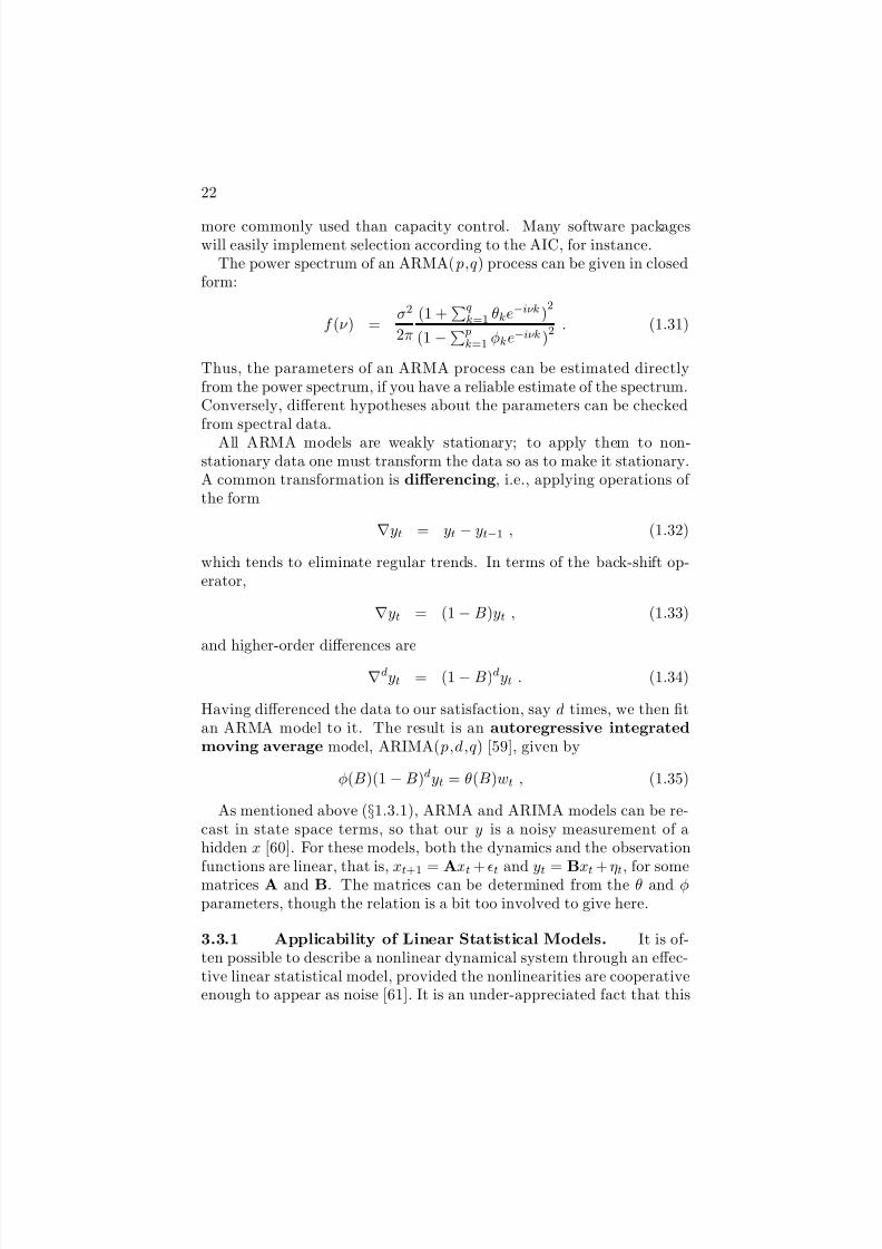
3.3.2 Extensions. While standard linear models are moreflexible than one might think, they do have their limits, and recognitionof this has spurred work on many extensions and variants. Here I brieflydiscuss a few of these.
Long Memory. The correlations of standard ARMA and ARIMAmodels decay fairly rapidly, in general exponentially; ρ(t) ∝ e−t/τ c ,where τ c is the correlation time. For some series, however, τ c is effectivelyinfinite, and ρ(t) ∝ t−α for some exponent α. These are called long-memory processes, because they remain substantially correlated oververy long times. These can still be accommodated within the ARIMAframework, formally, by introducing the idea of fractional differencing,or, in continuous time, fractional derivatives [64, 53]. Often long-memoryprocesses are self-similar, which can simplify their statistical estimation[65].
Volatility. All ARMA and even ARIMA models assume constant
variance. If the variance is itself variable, it can be worthwhile to modelit. Autoregressive conditionally heteroscedastic (ARCH) modelsassume a fixed mean value for yr, but a variance which is an auto-regression on y2
t . Generalized ARCH (GARCH) models expand theregression to include the (unobserved) earlier variances. ARCH andGARCH models are especially suitable for processes which display clus-tered volatility, periods of extreme fluctuation separated by stretchesof comparative calm.
Nonlinear and Nonparametric Models. Nonlinear models areobviously appealing, and when a particular parametric form of modelis available, reasonably straight-forward modifications of the linear ma-
chinery can be used to fit, evaluate and forecast the model [55, §4.9].However, it is often impractical to settle on a good parametric form be-forehand. In these cases, one must turn to nonparametric models, asdiscussed in §1.2.2; neural networks are a particular favorite here [35].The so-called kernel smoothing methods are also particularly well-developed for time series, and often perform almost as well as parametricmodels [66]. Finally, information theory provides universal prediction

8/6/2019 Methods and Techniques of complex system science
http://slidepdf.com/reader/full/methods-and-techniques-of-complex-system-science 24/96
24
methods, which promise to asymptotically approach the best possibleprediction, starting from exactly no background knowledge. This poweris paid for by demanding a long initial training phase used to infer thestructure of the process, when predictions are much worse than manyother methods could deliver [67].
3.4 The Nonlinear Dynamics Approach
The younger approach to the analysis of time series comes from nonlin-ear dynamics, and is intimately bound up with the state-space approachdescribed in §1.3.1 above. The idea is that the dynamics on the statespace can be determined directly from observations, at least if certain
conditions are met.The central result here is the Takens Embedding Theorem [68]; a
simplified, slightly inaccurate version is as follows. Suppose the d-dimensional state vector xt evolves according to an unknown but con-tinuous and (crucially) deterministic dynamic. Suppose, too, that theone-dimensional observable y is a smooth function of x, and “coupled”to all the components of x. Now at any time we can look not just atthe present measurement y(t), but also at observations made at timesremoved from us by multiples of some lag τ : yt−τ , yt−2τ , etc. If we usek lags, we have a k-dimensional vector. One might expect that, as thenumber of lags is increased, the motion in the lagged space will becomemore and more predictable, and perhaps in the limit k
→ ∞would be-
come deterministic. In fact, the dynamics of the lagged vectors becomedeterministic at a finite dimension; not only that, but the deterministicdynamics are completely equivalent to those of the original state space!(More exactly, they are related by a smooth, invertible change of coor-dinates, or diffeomorphism.) The magic embedding dimension k isat most 2d + 1, and often less.
Given an appropriate reconstruction via embedding, one can investi-gate many aspects of the dynamics. Because the reconstructed space isrelated to the original state space by a smooth change of coordinates,any geometric property which survives such treatment is the same forboth spaces. These include the dimension of the attractor, the Lyapunovexponents (which measure the degree of sensitivity to initial conditions)and certain qualitative properties of the autocorrelation function andpower spectrum (“correlation dimension”). Also preserved is the rela-tion of “closeness” among trajectories — two trajectories which are closein the state space will be close in the embedding space, and vice versa.This leads to a popular and robust scheme for nonlinear prediction, themethod of analogs: when one wants to predict the next step of the

8/6/2019 Methods and Techniques of complex system science
http://slidepdf.com/reader/full/methods-and-techniques-of-complex-system-science 25/96
Overview of Methods and Techniques 25
series, take the current point in the embedding space, find a similarone with a known successor, and predict that the current point will dothe analogous thing. Many refinements are possible, such as taking aweighted average of nearest neighbors, or selecting an analog at random,with a probability decreasing rapidly with distance. Alternately, one cansimply fit non-parametric predictors on the embedding space. (See [69]for a review.) Closely related is the idea of noise reduction, usingthe structure of the embedding-space to filter out some of the effects of measurement noise. This can work even when the statistical characterof the noise is unknown (see [69] again).
Determining the number of lags, and the lag itself, is a problem of
model selection, just as in §1.2, and can be approached in that spirit.An obvious approach is to minimize the in-sample forecasting error, aswith ARMA models; recent work along these lines [70, 71] uses the mini-mum description length principle (described in §1.8.3.1 below) to controlover-fitting. A more common procedure for determining the embeddingdimension, however, is the false nearest neighbor method [72]. Theidea is that if the current embedding dimension k is sufficient to resolvethe dynamics, k + 1 would be too, and the reconstructed state space willnot change very much. In particular, points which were close together inthe dimension-k embedding should remain close in the dimension-k + 1embedding. Conversely, if the embedding dimension is too small, pointswhich are really far apart will be brought artificially close together (just
as projecting a sphere on to a disk brings together points on the oppo-site side of a sphere). The particular algorithm of Kennel et al., whichhas proved very practical, is to take each point in the k-dimensional em-bedding, find its nearest neighbor in that embedding, and then calculatethe distance between them. One then calculates how much further apartthey would be if one used a k + 1-dimensional embedding. If this extradistance is more than a certain fixed multiple of the original distance,they are said to be “false nearest neighbors”. (Ratios of 2 to 15 arecommon, but the precise value does not seem to matter very much.)One then repeats the process at dimension k + 1, stopping when theproportion of false nearest neighbors becomes zero, or at any rate suf-ficiently small. Here, the loss function used to guide model selection is
the number of false nearest neighbors, and the standard prescriptionsamount to empirical risk minimization. One reason simple ERM workswell here is that the problem is intrinsically finite-dimensional (via theTakens result).
Unfortunately, the data required for calculations of quantities like di-mensions and exponents to be reliable can be quite voluminous. Approx-imately 102+0.4D data-points are necessary to adequately reconstruct an

8/6/2019 Methods and Techniques of complex system science
http://slidepdf.com/reader/full/methods-and-techniques-of-complex-system-science 26/96
8/6/2019 Methods and Techniques of complex system science
http://slidepdf.com/reader/full/methods-and-techniques-of-complex-system-science 27/96
Overview of Methods and Techniques 27
infinite number of dimensions, which is correct in a way, but definitelynot helpful.
These remarks should not be taken to belittle the very real powerof nonlinear dynamics methods. Applied skillfully, they are powerfultools for understanding the behavior of complex systems, especially forprobing aspects of their structure which are not directly accessible.
3.5 Filtering and State Estimation
Suppose we have a state-space model for our time series, and someobservations y, can we find the state x? This is the problem of filteringor state estimation. Clearly, it is not the same as the problem of
finding a model in the first place, but it is closely related, and also aproblem in statistical inference.
In this context, a filter is a function which provides an estimate xt of xt on the basis of observations up to and including10 time t: xt = f (yt0).A filter is recursive11 if it estimates the state at t on the basis of itsestimate at t − 1 and the new observation: xt = f (xt−1, yt). Recursivefilters are especially suited to on-line use, since one does not need toretain the complete sequence of previous observations, merely the mostrecent estimate of the state. As with prediction in general, filters can bedesigned to provide either point estimates of the state, or distributionalestimates. Ideally, in the latter case, we would get the conditional dis-tribution, Pr(X t = x
|Y t1 = yt1), and in the former case the conditional
expectation, x xPr(X t = x|Y t1 = yt1)dx.
Given the frequency with which the problem of state estimation showsup in different disciplines, and its general importance when it does ap-pear, much thought has been devoted to it over many years. The problemof optimal linear filters for stationary processes was solved independentlyby two of the “grandfathers” of complex systems science, Norbert Wienerand A. N. Kolmogorov, during the Second World War [78, 79]. In the1960s, Kalman and Bucy [80–82] solved the problem of optimal recur-sive filtering, assuming linear dynamics, linear observations and additivenoise. In the resulting Kalman filter, the new estimate of the state isa weighted combination of the old state, extrapolated forward, and thestate which would be inferred from the new observation alone. The re-quirement of linear dynamics can be relaxed slightly with what’s calledthe “extended Kalman filter”, essentially by linearizing the dynamicsaround the current estimated state.
Nonlinear solutions go back to pioneering work of Stratonovich [83]and Kushner [84] in the later 1960s, who gave optimal, recursive solu-tions. Unlike the Wiener or Kalman filters, which give point estimates,
8/6/2019 Methods and Techniques of complex system science
http://slidepdf.com/reader/full/methods-and-techniques-of-complex-system-science 28/96
28
the Stratonovich-Kushner approach calculates the complete conditionaldistribution of the state; point estimates take the form of the mean orthe most probable state [85]. In most circumstances, the strictly optimalfilter is hopelessly impractical numerically. Modern developments, how-ever, have opened up some very important lines of approach to practicalnonlinear filters [86], including approaches which exploit the geometryof the nonlinear dynamics [87, 88], as well as more mundane methodswhich yield tractable numerical approximations to the optimal filters[89, 90]. Noise reduction methods (§1.3.4) and hidden Markov models(§1.3.6) can also be regarded as nonlinear filters.
3.6 Symbolic or Categorical Time SeriesThe methods we have considered so far are intended for time-series
taking continuous values. An alternative is to break the range of thetime-series into discrete categories (generally only finitely many of them);these categories are sometimes called symbols, and the study of thesetime-series symbolic dynamics. Modeling and prediction then reducesto a (perhaps more tractable) problem in discrete probability, and manymethods can be used which are simply inapplicable to continuous-valuedseries [10]. Of course, if a bad discretization is chosen, the results of such methods are pretty well meaningless, but sometimes one gets datawhich is already nicely discrete — human languages, the sequences of bio-polymers, neuronal spike trains, etc. We shall return to the issue
of discretization below, but for the moment, we will simply considerthe applicable methods for discrete-valued, discrete-time series, howeverobtained.
Formally, we take a continuous variable z and partition its rangeinto a number of discrete cells, each labeled by a different symbol fromsome alphabet; the partition gives us a discrete variable y = φ(z). Aword or string is just a sequence of symbols, y0y1 . . . yn. A time serieszn0 naturally generates a string φ(zn0 ) ≡ φ(z0)φ(z1) . . . φ(zn). In general,not every possible string can actually be generated by the dynamics of the system we’re considering. The set of allowed sequences is called thelanguage. A sequence which is never generated is said to be forbidden.In a slightly inconsistent metaphor, the rules which specify the allowedwords of a language are called its grammar. To each grammar therecorresponds an abstract machine or automaton which can determinewhether a given word belongs to the language, or, equivalently, generateall and only the allowed words of the language. The generative versionsof these automata are stochastic, i.e., they generate different words withdifferent probabilities, matching the statistics of φ(z).
8/6/2019 Methods and Techniques of complex system science
http://slidepdf.com/reader/full/methods-and-techniques-of-complex-system-science 29/96
Overview of Methods and Techniques 29
By imposing restrictions on the forms the grammatical rules can take,or, equivalently, on the memory available to the automaton, we can di-vide all languages into four nested classes, a hierarchical classificationdue to Chomsky [91]. At the bottom are the members of the weakest,most restricted class, the regular languages generated by automatawithin only a fixed, finite memory for past symbols (finite state ma-chines). Above them are the context free languages, whose grammarsdo not depend on context; the corresponding machines are stack au-tomata, which can store an unlimited number of symbols in their mem-ory, but on a strictly first-in, first-out basis. Then come the context-sensitive languages; and at the very top, the unrestricted languages,
generated by universal computers. Each stage in the hierarchy can sim-ulate all those beneath it.We may seem to have departed very far from dynamics, but actually
this is not so. Because different languages classes are distinguished bydifferent kinds of memories, they have very different correlation prop-erties (§1.3.2), mutual information functions (§1.7), and so forth — see[10] for details. Moreover, it is often easier to determine these proper-ties from a system’s grammar than from direct examination of sequencestatistics, especially since specialized techniques are available for gram-matical inference [92, 93].
3.6.1 Hidden Markov Models. The most important special
case of this general picture is that of regular languages. These, we said,are generated by machines with only a finite memory. More exactly,there is a finite set of states x, with two properties:
1 The distribution of yt depends solely on xt, and
2 The distribution of xt+1 depends solely on xt.
That is, the x sequence is a Markov chain, and the observed y sequenceis noisy function of that chain. Such models are very familiar in signalprocessing [94], bioinformatics [95] and elsewhere, under the name of hidden Markov models (HMMs). They can be thought of as a gener-alization of ordinary Markov chains to the state-space picture describedin
§1.3.1. HMMs are particularly useful in filtering applications, since
very efficient algorithms exist for determining the most probable valuesof x from the observed sequence y. The expectation-maximization(EM) algorithm [96] even allows us to simultaneously infer the mostprobable hidden states and the most probable parameters for the model.
3.6.2 Variable-Length Markov Models. The main limita-tion of ordinary HMMs methods, even the EM algorithm, is that they

8/6/2019 Methods and Techniques of complex system science
http://slidepdf.com/reader/full/methods-and-techniques-of-complex-system-science 30/96
30
assume a fixed architecture for the states, and a fixed relationshipbetween the states and the observations. That is to say, they are notgeared towards inferring the structure of the model. One could applythe model-selection techniques of §1.2, but methods of direct inferencehave also been developed. A p opular one relies on variable-lengthMarkov models, also called context trees or probabilistic suffixtrees [97–100].
A suffix here is the string at the end of the y time series at a giventime, so e.g. the binary series abbabbabb has suffixes b, bb, abb, babb,etc., but not bab. A suffix is a context if the future of the series isindependent of its past, given the suffix. Context-tree algorithms try
to identify contexts by iteratively considering longer and longer suffixes,until they find one which seems to be a context. For instance, in a binaryseries, such an algorithm would first try whether the suffices a and b arecontexts, i.e., whether the conditional distribution Pr(Y t+1|Y t = a) canbe distinguished from Pr(Y t+1|Y t = a, Y −
t−1), and likewise for Y t = b. Itcould happen that a is a context but b is not, in which case the algorithmwill try ab and bb, and so on. If one sets xt equal to the context at timet, xt is a Markov chain. This is called a variable-length Markov modelbecause the contexts can be of different lengths.
Once a set of contexts has been found, they can be used for prediction.Each context corresponds to a different distribution for one-step-aheadpredictions, and so one just needs to find the context of the current time
series. One could apply state-estimation techniques to find the context,but an easier solution is to use the construction process of the contextsto build a decision tree (§1.2.2), where the first level looks at Y t, thesecond at Y t−1, and so forth.
Variable-length Markov models are conceptually simple, flexible, fast,and frequently more accurate than other ways of approaching the sym-bolic dynamics of experimental systems [101]. However, not every reg-ular language can be represented by a finite number of contexts. Thisweakness can be remedied by moving to a more powerful class of models,discussed next.
3.6.3 Causal-State Models, Observable-Operator Models,
and Predictive-State Representations. In discussing the state-space picture in §1.3.1 above, we saw that the state of a system is basi-cally defined by specifying its future time-evolution, to the extent thatit can be specified. Viewed in this way, a state X t corresponds to a dis-tribution over future observables Y +t+1. One natural way of finding suchdistributions is to look at the conditional distribution of the future obser-vations, given the previous history, i.e., Pr(Y +t+1|Y −
t = y−t ). For a given

8/6/2019 Methods and Techniques of complex system science
http://slidepdf.com/reader/full/methods-and-techniques-of-complex-system-science 31/96
Overview of Methods and Techniques 31
stochastic process or dynamical system, there will be a certain charac-teristic family of such conditional distributions. One can then considerthe distribution-valued process generated by the original, observed pro-cess. It turns out that the former has is always a Markov process, andthat the original process can be expressed as a function of this Markovprocess plus noise. In fact, the distribution-valued process has all theproperties one would want of a state-space model of the observations.The conditional distributions, then, can be treated as states.
This remarkable fact has lead to techniques for modeling discrete-valued time series, all of which attempt to capture the conditional-distribution states, and all of which are strictly more powerful than
VLMMs. There are at least three: the causal-state models or causal-state machines (CSMs)12 introduced by Crutchfield and Young [102],the observable operator models (OOMs) introduced by Jaeger [103],and the predictive state representations (PSRs) introduced by Littman,Sutton and Singh [104]. The simplest way of thinking of such objects isthat they are VLMMs where a context or state can contain more thanone suffix, adding expressive power and allowing them to give compactrepresentations of a wider range of processes. (See [105] for more on thispoint, with examples.)
All three techniques — CSMs, OOMs and PSRs — are basically equiv-alent, though they differ in their formalisms and their emphases. CSMsfocus on representing states as classes of histories with the same condi-
tional distributions, i.e., as suffixes sharing a single context. (They alsofeature in the “statistical forecasting” approach to measuring complex-ity, discussed in §1.8.3.2 b elow.) OOMs are named after the operatorswhich update the state; there is one such operator for each possible ob-servation. PSRs, finally, emphasize the fact that one does not actuallyneed to know the probability of every possible string of future obser-vations, but just a restricted sub-set of key trajectories, called “tests”.In point of fact, all of them can be regarded as special cases of moregeneral prior constructions due to Salmon (“statistical relevance basis”)[106, 107] and Knight (“measure-theoretic prediction process”) [48, 49],which were themselves independent. (This area of the literature is morethan usually tangled.)
Efficient reconstruction algorithms or discovery procedures ex-ist for building CSMs [105] and OOMs [103] directly from data. (Thereis currently no such discovery procedure for PSRs, though there areparameter-estimation algorithms [108].) These algorithms are reliable,in the sense that, given enough data, the probability that they build thewrong set of states becomes arbitrarily small. Experimentally, selecting
8/6/2019 Methods and Techniques of complex system science
http://slidepdf.com/reader/full/methods-and-techniques-of-complex-system-science 32/96
32
an HMM architecture through cross-validation never does better thanreconstruction, and often much worse [105].
While these models are more powerful than VLMMs, there are stillmany stochastic processes which cannot be represented in this form;or, rather, their representation requires an infinite number of states[109, 110]. This is mathematically unproblematic, though reconstructionwill then become much harder. (For technical reasons, it seems likelyto be easier to carry through for OOMs or PSRs than for CSMs.) Infact, one can show that these techniques would work straight-forwardlyon continuous-valued, continuous-time processes, if only we knew thenecessary conditional distributions [48, 111]. Devising a reconstruction
algorithm suitable for this setting is an extremely challenging and com-pletely unsolved problem; even parameter estimation is difficult, andcurrently only possible under quite restrictive assumptions [112].
3.6.4 Generating Partitions. So far, everything has assumedthat we are either observing truly discrete quantities, or that we have afixed discretization of our continuous observations. In the latter case, itis natural to wonder how much difference the discretization makes. Theanswer, it turns out, is quite a lot ; changing the partition can lead tocompletely different symbolic dynamics [113–115]. How then might wechoose a good partition?
Nonlinear dynamics provides an answer, at least for deterministic
systems, in the idea of a generating partition [10, 116]. Supposewe have a continuous state x and a deterministic map on the stateF , as in §1.3.1. Under a partitioning φ, each point x in the statespace will generate an infinite sequence of symbols, Φ(x), as follows:φ(x), φ(F (x)), φ(F 2(x)), . . .. The partition φ is generating if each pointx corresponds to a unique symbol sequence, i.e., if Φ is invertible. Thus,no information is lost in going from the continuous state to the discretesymbol sequence13. While one must know the continuous map F to de-termine exact generating partitions, there are reasonable algorithms forapproximating them from data, particularly in combination with em-bedding methods [75, 117, 118]. When the underlying dynamics arestochastic, however, the situation is much more complicated [119].
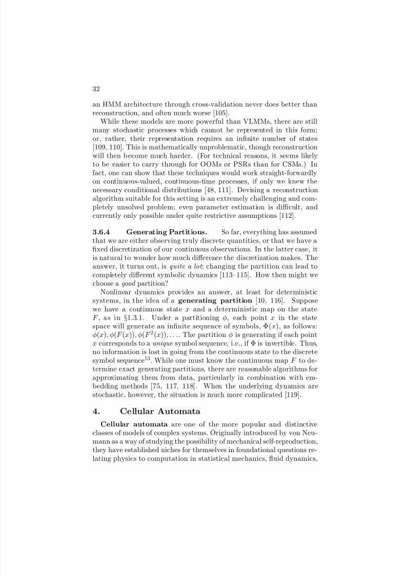
4. Cellular Automata
Cellular automata are one of the more popular and distinctiveclasses of models of complex systems. Originally introduced by von Neu-mann as a way of studying the possibility of mechanical self-reproduction,they have established niches for themselves in foundational questions re-lating physics to computation in statistical mechanics, fluid dynamics,

8/6/2019 Methods and Techniques of complex system science
http://slidepdf.com/reader/full/methods-and-techniques-of-complex-system-science 33/96
Overview of Methods and Techniques 33
and pattern formation. Within that last, perhaps the most relevant tothe present purpose, they have been extensively and successfully ap-plied to physical and chemical pattern formation, and, somewhat morespeculatively, to biological development and to ecological dynamics. In-teresting attempts to apply them to questions like the development of cities and regional economies lie outside the scope of this chapter.
4.1 A Basic Explanation of CA
Take a board, and divide it up into squares, like a chess-board orchecker-board. These are the cells. Each cell has one of a finite numberof distinct colors — red and black, say, or (to be patriotic) red, white
and blue. (We do not allow continuous shading, and every cell has justone color.) Now we come to the “automaton” part. Sitting somewhereto one side of the board is a clock, and every time the clock ticks thecolors of the cells change. Each cell looks at the colors of the nearby cells,and its own color, and then applies a definite rule, the transition rule,specified in advance, to decide its color in the next clock-tick; and all thecells change at the same time. (The rule can say “Stay the same.”) Eachcell is a sort of very stupid computer — in the jargon, a finite-stateautomaton — and so the whole board is called a cellular automaton,or CA. To run it, you color the cells in your favorite pattern, start theclock, and stand back.
Let us follow this concrete picture with one more technical and ab-
stract. The cells do not have to be colored, of course; all that’s importantis that each cell is in one of a finite number of states at any given time.By custom they’re written as the integers, starting from 0, but any “fi-nite alphabet” will do. Usually the number of states is small, underten, but in principle any finite number is allowed. What counts as the“nearby cells”, the neighborhood, varies from automaton to automa-ton; sometimes just the four cells on the principle directions, sometimesthe corner cells, sometimes a block or diamond of larger size; in principleany arbitrary shape. You do not need to stick to a chess-board; you canuse any regular pattern of cells which will fill the plane (or “tessellate”it; an old name for cellular automata is tessellation structures). Andyou do not have to stick to the plane; any number of dimensions is al-lowed. There are various tricks for handling the edges of the space; theone which has “all the advantages of theft over honest toil” is to assumean infinite board.
Cellular Automata as Parallel Computers. CA are syn-chronous massively parallel computers, with each cell being a finitestate transducer, taking input from its neighbors and making its own

8/6/2019 Methods and Techniques of complex system science
http://slidepdf.com/reader/full/methods-and-techniques-of-complex-system-science 34/96
34
state available as output. From this perspective, the remarkable thingabout CA is that they are computationally universal, able to calculateany (classically) computable function; one can use finite-state machines,the least powerful kind of computer, to build devices equivalent to Tur-ing machines, the most powerful kind of computer. The computationalpower of different physically-motivated CA is an important topic in com-plex systems [120, 121], though it must be confessed that CA with verydifferent computational powers can have very similar behavior in mostrespects.
Cellular Automata as Discrete Field Theories. From the per-
spective of physics, a CA is a “digitized” classical field theory, in whichspace, time and the field (state) are all discrete. Thus fluid mechan-ics, continuum mechanics, and electromagnetism can all be simulatedby CA14 typically, however, the physical relevance of a CA comes notfrom accurately simulating some field theory at the microscopic level,but from the large-scale phenomena they generate.
Take, for example, simulating fluid mechanics, where CA are alsocalled lattice gases or lattice fluids. In the “HPP” [122] rule, a typi-cal lattice gas with a square grid, there are four species of “fluid particle”,which travel along the four principal directions. If two cells moving inopposite directions try to occupy the same location at the same time,they collide, and move off at right angles to their original axis (Figure
1.4). Each cell thus contains only an integer number of particles, andonly a discrete number of values of momentum are possible. If one takesaverages over reasonably large regions, however, then density and mo-mentum approximately obey the equations of continuous fluid mechan-ics. Numerical experiments show that this rule reproduces many fluidphenomena, such as diffusion, sound, shock-waves, etc. However, withthis rule, the agreement with fluid mechanics is only approximate. Inparticular, the square lattice makes the large-scale dynamics anisotropic,which is unphysical. This in turn can be overcome in several ways — forinstance, by using a hexagonal lattice [123]. The principle here — getthe key parts of the small-scale “microphysics” right, and the interesting“macrophysics” will take care of itself — is extensively applied in study-
ing pattern formation, including such biologically-relevant phenomenaas phase separation [124], excitable media [125], and the self-assemblyof micelles [126, 127].
5. Agent-Based Models
If there is any one technique associated with complex systems science,it is agent-based modeling. An agent-based model is a computational
8/6/2019 Methods and Techniques of complex system science
http://slidepdf.com/reader/full/methods-and-techniques-of-complex-system-science 35/96
Overview of Methods and Techniques 35
Figure 1.4. Collisions in the HPP lattice gas rule. Horizontal collisions producevertically-moving particles (top) and vice versa (middle). Particles moving at rightangles pass by each other unchanged (bottom, omitting the reflections and rotationsof this figure).
model which represents individual agents and their collective behavior.What, exactly, do we mean by “agent”? Stuart Kauffman has offered15
the following apt definition: “An agent is a thing which does things tothings”. That is, an agent is a persistent thing which has some state we
find worth representing, and which interacts with other agents, mutu-ally modifying each others’ states. The components of an agent-basedmodel are a collection of agents and their states, the rules governingthe interactions of the agents, and the environment within which theylive. (The environment need not be represented in the model if its ef-fects are constant.) The state of an agent can be arbitrarily simple, say just position, or the color of a cell in a CA. (At this end, agent-basedmodels blend with traditional stochastic models.) States can also be ex-tremely complicated, including, possibly, sophisticated internal modelsof the agent’s world.
Here is an example to make this concrete. In epidemiology, there isa classic kind of model of the spread of a disease through a populationcalled an “SIR” model [128, §4.4]. It has three classes of people — thesusceptible, who have yet to be exposed to the disease; the infected,who have it and can pass it on; and the resistant or recovered, who havesurvived the disease and cannot be re-infected. A traditional approachto an SIR model would have three variables, namely the number of people in each of the three categories, S (t), I (t), R(t), and would havesome deterministic or stochastic dynamics in terms of those variables.

8/6/2019 Methods and Techniques of complex system science
http://slidepdf.com/reader/full/methods-and-techniques-of-complex-system-science 36/96
8/6/2019 Methods and Techniques of complex system science
http://slidepdf.com/reader/full/methods-and-techniques-of-complex-system-science 37/96
Overview of Methods and Techniques 37
Agent-based models steer you towards representing individuals, theirbehaviors and their interactions, rather than aggregates and their dy-namics. Whether this is a good thing depends, of course, on what youknow, and what you hope to learn. If you know a lot about individuals,agent-based models can help you leverage that knowledge into informa-tion about collective dynamics. This is particularly helpful if the pop-ulation is heterogeneous, since you can represent the different types of individuals in the population by different states for agents. This requiresa bit of effort on your part, but often not nearly so much as it wouldto represent the heterogeneity in an aggregated model. Conversely, if you think you have the collective dynamics down, an ABM will let you
check whether a candidate for an individual-level mechanism really willproduce them. (But see §1.6, below.)Ideally, there are no “mass nouns” in an ABM, nothing represented by
a smeared-out “how much”: everything should be represented by somedefinite number of distinctly-located agents. At most, some aggregatevariables may be stuffed into the environment part of the model, but onlysimple and homogeneous ones. Of course, the level of disaggregation atwhich it is useful to call something an agent is a matter for particularapplications, and need not be the same for every agent in a model.(E.g., one might want to model an entire organ as a single agent, whileanother, more interesting organ is broken up into multiple interactingagents, along anatomical or functional lines.) Sometimes it’s just not
practical to represent everything which we know is an individual thingby its own agent: imagine trying to do chemical thermodynamics bytracking the interactions of a mole of molecules. Such cases demandeither giving up on agent-based modeling (fortunately, the law of massaction works pretty well in chemistry), or using fictitious agents thatrepresent substantial, but not too large, collections of individuals.
Models describing the collective dynamics of aggregate variables aresometimes called “equation-based models”, in contrast to agent-basedmodels. This is sloppy, however: it is always possible, though gener-ally tedious and unilluminating, to write down a set of equations whichdescribe the dynamics of an agent-based model. Rather than drawinga false contrast between agents and equations, it would b e better to
compare ABMs to “aggregate models”, “collective models” or perhaps“factor models”.
8/6/2019 Methods and Techniques of complex system science
http://slidepdf.com/reader/full/methods-and-techniques-of-complex-system-science 38/96
38
5.1 Computational Implementation: Agents areObjects
The nicest way to computationally implement the commitment of dis-tinctly representing each agent, is to make agents objects, which are,to over-simplify slightly, data structures which have internal states, andinteract with each other by passing messages. While objects are not nec-essary for agent-based models, they do make programming them much easier, especially if the agents have much more state than, say, just aposition and a type. If you try to implement models with sophisticatedagents without using objects, the odds are good that you will find your-self re-inventing well-known features of object-oriented programming.
(Historically, object-oriented programming began with languages for sim-ulation modeling [131].) You might as well save your time, and do thosethings right , by using objects in the first place.
Generally speaking, computational implementations of ABMs containmany non-agent objects, engaged in various housekeeping tasks, or im-plementing the functions agents are supposed to perform. For instance,an agent, say a rat, might be supposed to memorize a sequence, sayof turns in a maze. One way of implementing this would be to use alinked list, which is an object itself. Such objects do not represent actualfeatures of the model , and it should be possible to vary them withoutinterfering with the model’s behavior. Which objects are picked out asagents is to some degree a matter of convenience and taste. It is common,for instance, to have mobile agents interacting on a static environment.If the environment is an object, modelers may or may not speak of itas an “environment agent,” and little seems to hinge on whether or notthey do.
There are several programming environments designed to facilitateagent-based modeling. Perhaps the best known of these is Swarm(www.swarm.org), which works very flexibly with several languages, isextensively documented, and has a large user community, though itpresently (2004) lacks an institutional home. RePast, while concep-tually similar, is open-source (repast.sourceforge.net ) and is asso-ciated with the University of Chicago. StarLogo, and it successor,NetLogo
(ccl.sesp.northwestern.edu/netlogo ), are extensions of the popular Logo language to handle multiple interacting “turtles”, i.e.,agents. Like Logo, children can learn to use them [132], but they arefairly easy for adults, too, and certainly give a feel for working withABMs.

8/6/2019 Methods and Techniques of complex system science
http://slidepdf.com/reader/full/methods-and-techniques-of-complex-system-science 39/96
8/6/2019 Methods and Techniques of complex system science
http://slidepdf.com/reader/full/methods-and-techniques-of-complex-system-science 40/96
40
a long tradition of using highly simplified models as caricatures of realsystems.
All three motives are appropriate, in their place. (i) is completely un-exceptionable; abstracting away from irrelevant detail is always worth-while, so long as it really is irrelevant. (ii) is also fair enough, thoughone should be careful that the mechanisms in one’s model can still gen-erate the phenomenon when they interact with other effects as well.(iii) works very nicely in statistical physics itself, where there are pow-erful mathematical results relating to the renormalization group [139]and bifurcation theory [14] which allow one to extract certain kinds of quantitative results from simplified models which share certain qualita-
tive characteristics with real systems. (We have seen a related principlewhen discussing cellular automata models above.) There is, however, lit-tle reason to think that these universality results apply to most complexsystems, let alone ones with adaptive agents!
6. Evaluating Models of Complex Systems
We do not build models for their own sake; we want to see what theydo, and we want to compare what they do both to reality and to othermodels. This kind of evaluation of models is a problem for all areas of science, and as such little useful general advice can be given. However,there are some issues which are peculiar to models of complex systems,or especially acute for them, and I will try to provide some guidance
here, moving from figuring out just what your model does, to comparingyour model to data, to comparing it to other models.
6.1 Simulation
The most basic way to see what your model does is to run it; to do asimulation. Even though a model is entirely a human construct, everyaspect of its behavior following logically from its premises and initialconditions, the frailty of human nature is such that we generally cannotperceive those consequences, not with any accuracy. If the model in-volves a large number of components which interact strongly with eachother — if, that is to say, it’s a good model of a complex system — our
powers of deduction are generally overwhelmed by the mass of relevant,interconnected detail. Computer simulation then comes to our aid, be-cause computers have no trouble remembering large quantities of detail,nor in following instructions.
6.1.1 Direct Simulation. Direct simulation — simply startingthe model and letting it go — has two main uses. One is to get a sense
8/6/2019 Methods and Techniques of complex system science
http://slidepdf.com/reader/full/methods-and-techniques-of-complex-system-science 41/96
Overview of Methods and Techniques 41
of the typical b ehavior, or of the range of behavior. The other, morequantitative, use is to determine the distribution of important quan-tities, including time series. If one randomizes initial conditions, andcollects data over multiple runs, one can estimate the distribution of de-sired quantities with great accuracy. This is exploited in the time seriesmethod of surrogate data (above), but the idea applies quite generally.
Individual simulation runs for models of complex systems can be rea-sonably expensive in terms of time and computing power; large numbersof runs, which are really needed to have confidence in the results, arecorrespondingly more costly. Few things are more dispiriting than toexpend such quantities of time and care, only to end up with ambigu-
ous results. It is almost always worthwhile, therefore, to carefully thinkthrough what you want to measure, and why, before running anything.In particular, if you are trying to judge the merits of competing models,effort put into figuring out how and where they are most different willgenerally be well-rewarded. The theory of experimental design offersextensive guidance on how to devise informative series of experiments,both for model comparison and for other purposes, and by and large theprinciples apply to simulations as well as to real experiments.
6.1.2 Monte Carlo Methods. Monte Carlo is the nameof a broad, slightly indistinct family for using random processes to es-timate deterministic quantities, especially the properties of probability
distributions. A classic example will serve to illustrate the basic idea,on which there are many, many refinements.Consider the problem of determining the area A under an curve given
by a known but irregular function f (x). In principle, you could integratef to find this area, but suppose that numerical integration is infeasiblefor some reason. (We will come back to this p oint presently.) A MonteCarlo solution to this problem is as follows: pick points at random,uniformly over the square. The probability p that a point falls in theshaded region is equal to the fraction of the square occupied by theshading: p = A/s2. If we pick n points independently, and x of them fallin the shaded region, then x/n → p (by the law of large numbers), ands2x/n
→A. s2x/n provides us with a stochastic estimate of the integral.
Moreover, this is a probably approximately correct (§1.2.1.3) estimate,and we can expect, from basic probability theory, that the standarddeviation of the estimate around its true value will be proportional ton−1/2, which is not bad16. However, when faced with such a claim, oneshould always ask what the proportionality constant is, and whether itis the best achievable. Here it is not: the equally simple, if less visual,
8/6/2019 Methods and Techniques of complex system science
http://slidepdf.com/reader/full/methods-and-techniques-of-complex-system-science 42/96
42
scheme of just picking values of x uniformly and averaging the resultingvalues of f (x) always has a smaller standard deviation [140, chapter 5].
This example, while time-honored and visually clear, does not showMonte Carlo to its best advantage; there are few one-dimensional inte-grals which cannot be done better by ordinary, non-stochastic numer-ical methods. But numerical integration becomes computationally in-tractable when the domain of integration has a large number of dimen-sions, where “large” begins somewhere between four and ten. MonteCarlo is much more indifferent to the dimensionality of the space: wecould replicate our example with a 999-dimensional hyper-surface in a1000-dimensional space, and we’d still get estimates that converged like
n
−1/2
, so achieving an accuracy of ±ǫ will require evaluating the functionf only O(ǫ−2) times.Our example was artificially simple in another way, in that we used
a uniform distribution over the entire space. Often, what we want isto compute the expectation of some function f (x) with a non-uniformprobability p(x). This is just an integral,
f (x) p(x)dx, so we could
sample points uniformly and compute f (x) p(x) for each one. But if somepoints have very low probability, so they only make a small contributionto the integral, spending time evaluating the function there is a bit of a waste. A b etter strategy would be to pick points according to theactual probability distribution. This can sometimes be done directly,especially if p(x) is of a particularly nice form. A very general and
clever indirect scheme is as follows [141]. We want a whole sequence of points, x1, x2, . . . xn. We pick the first one however we like, and afterthat we pick successive p oints according to some Markov chain: thatis, the distribution of xi+1 depends only on xi, according to some fixedfunction q(xi, xi+1). Under some mild conditions17, the distribution of xt approaches a stationary distribution q∗(x) at large times t. If we couldensure that q∗(x) = p(x), we know that the Markov chain was convergingto our distribution, and then, by the ergodic theorem, averaging f (x)along a trajectory would give the expected value of f (x). One way toensure this is to use the “detailed balance” condition of the invariantdistribution, that the total probability of going from x to y must equalthe total probability of going the other way:
p(x)q(x, y) = p(y)q(y, x) (1.39)
q(x, y)
q(y, x)=
p(y)
p(x)≡ h(x, y) (1.40)
So now we just need to make sure that (1.40) is satisfied. One wayto do this is to set q(x, y) = min(1, h(x, y)); this was the original pro-
posal of Metropolis et al . Another is q(x, y) = h(x,y)1+h(x,y) . This method
8/6/2019 Methods and Techniques of complex system science
http://slidepdf.com/reader/full/methods-and-techniques-of-complex-system-science 43/96
Overview of Methods and Techniques 43
is what physicists usually mean by “Monte Carlo”, but statisticians callit Markov chain Monte Carlo, or “MCMC”. While we can now es-timate the properties of basically arbitrary distributions, we no longerhave independent samples, so evaluating the accuracy of our estimatesis no longer a matter of trivial probability18. An immense range of re-finements have been developed over the last fifty years, addressing theseand other points; see the further reading section for details.
Keep in mind that Monte Carlo is a stochastic simulation method onlyin a special sense — it simulates the probability distribution p(x), not themechanism which generated that distribution. The dynamics of Markovchain Monte Carlo, in particular, often bear no resemblance whatsoever
to those of the real system
19
. Since the point of Monte Carlo is to tellus about the properties of p(x) (what is the expectation value of thisfunction? what is the probability of configurations with this property?etc.), the actual trajectory of the Markov chain is of no interest. Thispoint sometimes confuses those more used to direct simulation methods.
6.2 Analytical Techniques
Naturally enough, analytical techniques are not among the tools whichfirst come to mind for dealing with complex systems; in fact, they oftendo not come to mind at all. This is unfortunate, because a lot of intel-ligence has been devoted to devising approximate analytical techniquesfor classes of models which include many of those commonly used for
complex systems. A general advantage of analytical techniques is thatthey are often fairly insensitive to many details of the model. Since anymodel we construct of a complex system is almost certainly much sim-pler than the system itself, a great many of its details are just wrong. If we can extract non-trivial results which are insensitive to those details,we have less reason to worry about this.
One particularly useful, yet neglected, body of approximate analyticaltechniques relies on the fact that many complex systems models areMarkovian. In an agent-based model, for instance, the next state of anagent generally depends only on its present state, and the present statesof the agents it interacts with. If there is a fixed interaction graph,the agents form a Markov random field on that graph. There are nowvery powerful and computationally efficient methods for evaluating manyproperties of Markov chains [58, 142], Markov random fields [143], and(closely related) graphical models [144] without simulation. The recentbooks of Peyton Young [145] and Sutton [146] provide nice instancesof using analytical results about Markov processes to solve models of complex social systems, without impractical numerical experiments.

8/6/2019 Methods and Techniques of complex system science
http://slidepdf.com/reader/full/methods-and-techniques-of-complex-system-science 44/96
44
6.3 Comparisons with Data
6.3.1 General issues. We can only compare particular aspectsof a model of a system to particular kinds of data about that system.The most any experimental test can tell us, therefore, is how similar themodel is to the system in that respect . One may think of an experimentalcomparison as a test for a particular kind of error , one of the infinitenumber of mistakes which we could make in building a model. A goodtest is one which is very likely to alert us to an error, if we have madeit, but not otherwise [50].
These ought to be things every school-child knows about testing hy-potheses. It is very easy, however, to blithely ignore these truisms when
confronted with, on the one hand, a system with many strongly inter-dependent parts, and, on the other hand, a model which tries to mirrorthat complexity. We must decide which features of the model ought tobe similar to the system, and how similar. It is important not only thatour model be able to adequately reproduce those phenomena, but that itnot entail badly distorted or non-existent phenomena in other respects.
6.3.2 Two Stories and Some Morals. Let me give twoexamples from very early in the study of complex systems, which nicelyillustrate some fundamental points.
The first has to do with pattern formation in chemical oscillators [147].Certain mixtures of chemicals in aqueous solution, mostly famously the
Belusov-Zhabotinsky reagent, can not only undergo cyclic chemical re-actions, but will form rotating spiral waves, starting from an initial fea-tureless state. This is a visually compelling example of self-organization,and much effort has been devoted to understanding it. One of the morepopular early models was the “Brusselator” advanced by Prigogine andhis colleagues at the Free University of Brussels; many similarly-namedvariants developed. Brusselator-type models correctly predicted thatthese media would support spiral waves. They all, further, predictedthat the spirals would form only when the homogeneous configurationwas unstable, and that then they would form spontaneously. It provedvery easy, however, to prepare the Belusov-Zhabotisnky reagent in sucha way that it was “perfectly stable in its uniform quiescence”, yet stillable to produce spiral waves if excited (e.g., by being touched with ahot wire) [148]. The Brusselator and its variants were simply unableto accommodate these phenomena, and had to be discarded in favor of other models. The fact that these were qualitative results, rather thanquantitative ones, if anything made it more imperative to get rid of theBrusselator.
8/6/2019 Methods and Techniques of complex system science
http://slidepdf.com/reader/full/methods-and-techniques-of-complex-system-science 45/96
Overview of Methods and Techniques 45
The second story concerns the work of Varela and Maturana on “au-topoesis”. In a famous paper [149], they claimed to exhibit a computa-tional model of a simple artificial chemistry where membranes not onlyformed spontaneously, but a kind of metabolism self-organized to sus-tain the membranes. This work influenced not just complex systemsscience but theoretical biology, psychology, and even sociology [150].When, in the 1990s, McMullin made the first serious effort to reproducethe results, based on the description of the model in the paper, thatdescription proved not to match the published simulation results. Thediscrepancy was only resolved by the fortuitous rediscovery of a massof papers, including Fortran code, that Varela had left behind in Chile
when forced into exile by the fascist regime. These revealed a crucialchange in one particular reaction made all the difference between suc-cessful autopoesis and its absence. (For the full story, see [151, 152].)Many similar stories could be told of other models in complex systems[153]; this one is distinguished by McMullin’s unusual tenacity in tryingto replicate the results, Varela’s admirable willingness to assist him, andthe happy ending.
The story of autopoesis is especially rich in morals. (1) Replication isessential. (2) It is a good idea to share not just data but programs. (3)Always test the robustness of your model to changes in its parameters.(This is fairly common.) (4) Always test your model for robustness tosmall changes in qualitative assumptions. If your model calls for a given
effect, there are usually several mechanisms which could accomplish it.If it does not matter which mechanism you actually use, the result is thatmuch more robust. Conversely, if it does matter, the over-all adequacy of the model can be tested by checking whether that mechanism is actuallypresent in the system. Altogether too few people perform such tests.
6.3.3 Comparing Macro-data and Micro-models. Dataare often available only about large aggregates, while models, especiallyagent-based models, are about individual behavior. One way of compar-ing such models to data is to compute the necessary aggregates, fromdirect simulation, Monte Carlo, etc. The problem is that many differentmodels can give the same aggregated behavior, so this does not provide
a powerful test between different models. Ideally, we’d work back fromaggregate data to individual behaviors, which is known, somewhat con-fusingly, as ecological inference. In general, the ecological inferenceproblem itself does not have a unique solution. But the aggregate data,if used intelligently, can often put fairly tight constraints on the indi-vidual behaviors, and micro-scale can be directly checked against thoseconstraints. Much of the work here has been done by social scientists, es-
8/6/2019 Methods and Techniques of complex system science
http://slidepdf.com/reader/full/methods-and-techniques-of-complex-system-science 46/96
46
pecially American political scientists concerned with issues arising fromthe Voting Rights Act [154], but the methods they have developed arevery general, and could profitably be applied to agent-based models inthe biological sciences, though, to my knowledge, they have yet to be.
6.4 Comparison to Other Models
Are there other ways of generating the data? There generally are,at least if “the data” are some very gross, highly-summarized pattern.This makes it important to look for differential signatures, places wherediscrepancies between different generative mechanisms give one someleverage. Given two mechanisms which can both account for our phe-
nomenon, we should look for some other quantity whose behavior willbe different under the two hypotheses. Ideally, in fact, we would look forthe statistic on which the two kinds of model are most divergent. The lit-erature on experimental design is relevant here again, since it considerssuch problems under the heading of model discrimination, seekingto maximize the power of experiments (or simulations) to distinguishbetween different classes of models [155, 156].
Perhaps no aspect of methodology is more neglected in complex sys-tems science than this one. While it is always perfectly legitimate toannounce a new mechanism as a way of generating a phenomenon, itis far too common for it to be called the way to do it, and vanishinglyrare to find an examination of how it differs from previously-proposed
mechanisms. Newman and Palmer’s work on extinction models [157]stands out in this regard for its painstaking examination of the ways of discriminating between the various proposals in the literature.
7. Information Theory
Information theory began as a branch of communications engineering,quantifying the length of codes needed to represent randomly-varyingsignals, and the rate at which data can be transmitted over noisy chan-nels. The concepts needed to solve these problems turn out to be quitefundamental measures of the uncertainty, variability, and the interde-pendence of different variables. Information theory thus is an important
tool for studying complex systems, and in addition is indispensable forunderstanding complexity measures (§1.8).
7.1 Basic Definitions
Our notation and terminology follows that of Cover and Thomas’sstandard textbook [158].

8/6/2019 Methods and Techniques of complex system science
http://slidepdf.com/reader/full/methods-and-techniques-of-complex-system-science 47/96
Overview of Methods and Techniques 47
Given a random variable X taking values in a discrete set A, theentropy or information content H [X ] of X is
H [X ] ≡ −a∈A
Pr(X = a)log2 Pr(X = a) . (1.41)
H [X ] is the expectation value of − log2 Pr(X ). It represents the un-certainty in X , interpreted as the mean number of binary distinctions(bits) needed to identify the value of X . Alternately, it is the minimumnumber of bits needed to encode or describe X . Note that H [X ] = 0 if and only if X is (almost surely) constant.
The joint entropy H [X, Y ] of two variables X and Y is the entropy
of their joint distribution:
H [X, Y ] ≡ −
a∈A,b∈B
Pr(X = a, Y = b)log2 Pr(X = a, Y = b) .(1.42)
The conditional entropy of X given Y is
H [X |Y ] ≡ H [X, Y ] − H [Y ] . (1.43)
H [X |Y ] is the average uncertainty remaining in X , given a knowledgeof Y .
The mutual information I [X ; Y ] between X and Y is
I [X ; Y ]≡
H [X ]−
H [X |Y ] . (1.44)
It gives the reduction in X ’s uncertainty due to knowledge of Y and issymmetric in X and Y . We can also define higher-order mutual infor-mations, such as the third-order information I [X ; Y ; Z ],
I [X ; Y ; Z ] ≡ H [X ] + H [Y ] + H [Z ] − H [X,Y,Z ] (1.45)
and so on for higher orders. These functions reflect the joint dependenceamong the variables.
Mutual information is a special case of the relative entropy, alsocalled the Kullback-Leibler divergence (or distance). Given twodistributions (not variables), P and Q, the entropy of Q relative to P is
D(PQ) ≡x
P(x)logP(x)
Q(x)(1.46)
D measures how far apart the two distributions are, since D(P||Q) ≥ 0,and D(PQ) = 0 implies the two distributions are equal almost every-where. The divergence can be interpreted either in terms of codes (seebelow), or in terms of statistical tests [159]. Roughly speaking, given n

8/6/2019 Methods and Techniques of complex system science
http://slidepdf.com/reader/full/methods-and-techniques-of-complex-system-science 48/96
48
samples drawn from the distribution P, the probability of our acceptingthe false hypothesis that the distribution is Q can go down no fasterthan 2−nD(PQ). The mutual information I [X ; Y ] is the divergence be-tween the joint distribution Pr(X, Y ), and the product of the marginaldistributions, Pr(X )Pr(Y ), and so measures the departure from inde-pendence.
Some extra information-theoretic quantities make sense for time seriesand stochastic processes. Supposing we have a process X =. . . , X −2, X −1, X 0, X 1, X 2, . . ., we can define its mutual informationfunction by analogy with the autocovariance function (see §1.3.2),
I X(s, t) = I [X s; X t] (1.47)
I X (τ ) = I [X t; X t+τ ] (1.48)
where the second form is valid only for strictly stationary processes.The mutual information function measures the degree to which differentparts of the series are dependent on each other.
The entropy rate h of a stochastic process
h ≡ limL→∞
H [X 0|X −1−L] (1.49)
= H [X 0|X −1−∞] . (1.50)
(The limit always exists for stationary processes.) h measures the pro-
cess’s unpredictability, in the sense that it is the uncertainty which re-mains in the next measurement even given complete knowledge of itspast. In nonlinear dynamics, h is called the Kolmogorov-Sinai (KS)entropy.
For continuous variables, one can define the entropy via an integral,
H [X ] ≡ −
p(x)log p(x)dx , (1.51)
with the subtlety that the continuous entropy not only can be negative,but depends on the coordinate system used for x. The relative entropyalso has the obvious definition,
D(PQ) ≡ p(x)log p(x)
q(x)dx (1.52)
but is coordinate-independent and non-negative. So, hence, is the mu-tual information.
Optimal Coding. One of the basic results of information theoryconcerns codes, or schemes for representing random variables by bit
8/6/2019 Methods and Techniques of complex system science
http://slidepdf.com/reader/full/methods-and-techniques-of-complex-system-science 49/96
Overview of Methods and Techniques 49
strings. That is, we want a scheme which associates each value of arandom variable X with a bit string. Clearly, if we want to keep theaverage length of our code-words small, we should give shorter codesto the more common values of X . It turns out that the average code-length is minimized if we use − log Pr(x) bits to encode x, and it isalways possible to come within one bit of this. Then, on average, we willuse E [− log Pr(x)] = H [X ] bits.
This presumes we know the true probabilities. If we think the true dis-tribution is Q when it is really P, we will, on average, use E [− log Q(x)] ≥H [X ]. This quantity is called the cross-entropy or inaccuracy, andis equal to H [X ] + D(PQ). Thus, finding the correct probability dis-
tribution is equivalent to minimizing the cross-entropy, or the relativeentropy [160].
The Khinchin Axioms and Renyi Information. In 1953, A. I.Khinchin published a list of four reasonable-looking axioms for a mea-sure of the information H [X ] associated with a random variable X [161].He then proved that the Shannon information was the unique functionalsatisfying the axioms, up to an over-all multiplicative constant. (Thechoice of this constant is equivalent to the choice of the base for loga-rithms.) The axioms were as follows.
The information is a functional of the probability distribution of X , and not on any of its other properties. In particular, if f is anyinvertible function, H [X ] = H [f (X )].
The information is maximal for the uniform distribution, where allevents are equally probable.
The information is unchanged by enlarging the probability spacewith events of zero probability.
If the probability space is divided into two sub-spaces, so that X is split into two variables Y and Z , the total information is equalto the information content of the marginal distribution of one sub-space, plus the mean information of the conditional distribution of
the other sub-space: H [X ] = H [Y ] + E [H (Z |Y )].A similar axiomatic treatment can be given for the mutual informationand the relative entropy.
While the first three of Khinchin’s axioms are all highly plausible, thefourth is somewhat awkward. It is intuitively more plausible to merelyrequire that, if Y and Z are independent, then H [Y, Z ] = H [Y ] + H [Z ].If the fourth axiom is weakened in this way, however, there is no longer
8/6/2019 Methods and Techniques of complex system science
http://slidepdf.com/reader/full/methods-and-techniques-of-complex-system-science 50/96
50
only a single functional satisfying the axioms. Instead, any of the infinitefamily of entropies introduced by Renyi satisfies the axioms. The Renyientropy of order α, with α any non-negative real number, is
H α[X ] ≡ 1
1 − αlog
i: pi>0
pαi (1.53)
in the discrete case, and the corresponding integral in the continuouscase. The parameter α can be thought of as gauging how stronglythe entropy is biased towards low-probability events. As α → 0, low-probability events count more, until at α = 0, all possible events receiveequal weight. (This is sometimes called the topological entropy.) As
α → ∞, only the highest-probability event contributes to the sum. Onecan show that, as α → 1, H α[X ] → H [X ], i.e., one recovers the ordinaryShannon entropy in the limit. There are entropy rates corresponding toall the Renyi entropies, defined just like the ordinary entropy rate. Fordynamical systems, these are related to the fractal dimensions of theattractor [162, 163].
The Renyi divergences bear the same relation to the Renyi en-tropies as the Kullback-Leibler divergence does to the Shannon entropy.The defining formula is
Dα(P||Q) ≡ 1
α − 1log
qi
piqi
α(1.54)
and similarly for the continuous case. Once again, limα→1 Dα(P||Q) =D(P||Q). For all α > 0, Dα(P||Q) ≥ 0, and is equal to zero if and onlyif P and Q are the same. (If α = 0, then a vanishing Renyi divergenceonly means that the supports of the two distributions are the same.) TheRenyi entropy H α[X ] is non-increasing as α grows, whereas the Renyidivergence Dα(P||Q) is non-decreasing.
Estimation of Information-Theoretic Quantities. In applica-tions, we will often want to estimate information-theoretic quantities,such as the Shannon entropy or the mutual information, from empiricalor simulation data. Restricting our attention, for the moment, to thecase of discrete-valued variables, the empirical distribution will gener-ally converge on the true distribution, and so the entropy (say) of theempirical distribution (“sample entropy”) will also converge on the trueentropy. However, it is not the case that the sample entropy is an unbi-ased estimate of the true entropy. The Shannon (and Renyi) entropiesare measures of variation, like the variance, and sampling tends to reducevariation. Just as the sample variance is a negatively biased estimate of the true variance, sample entropy is a negatively-biased estimate of the
8/6/2019 Methods and Techniques of complex system science
http://slidepdf.com/reader/full/methods-and-techniques-of-complex-system-science 51/96
Overview of Methods and Techniques 51
true entropy, and so sample mutual information is a positively-biasedestimate of true information. Understanding and controlling the bias,as well as the sampling fluctuations, can be very important.
Victor [164] has given an elegant method for calculating the bias of the sample entropy; remarkably, the leading-order term depends only onthe alphabet size k and the number of samples N , and is (k − 1)/2N .Higher-order terms, however, depend on the true distribution. Recently,Kraskov et al. [165] have published an adaptive algorithm for estimatingmutual information, which has very good properties in terms of both biasand variance. Finally, the estimation of entropy rates is a somewhattricky matter. The best practices are to either use an algorithm of
the type given by [166], or to fit a properly dynamical model. (Fordiscrete data, variable-length Markov chains, discussed in §1.3.6.2 above,generally work very well, and the entropy rate can be calculated fromthem very simply.) Another popular approach is to run one’s time seriesthrough a standard compression algorithm, such as gzip, dividing thesize in bits of the output by the number of symbols in the input [167].This is an absolutely horrible idea; even under the circumstances underwhich it gives a consistent estimate of the entropy rate, it convergesmuch more slowly, and runs more slowly, than employing either of thetwo techniques just mentioned [168, 169].20
7.2 Applications of Information Theory
Beyond its original home in communications engineering, informa-tion theory has found a multitude of applications in statistics [159, 160]and learning theory [144, 170]. Scientifically, it is very natural to con-sider some biological systems as communications channels, and so ana-lyze their information content; this has been particularly successful forbiopolymer sequences [171] and especially for neural systems, where theanalysis of neural codes depends vitally on information theory [172, 173].However, there is nothing prohibiting the application of information the-ory to systems which are not designed to function as communicationsdevices; the concepts involved require only well-defined probability dis-tributions. For instance, in nonlinear dynamics [174, 175] information-theoretic notions are very important in characterizing different kinds of dynamical system (see also §1.3.6). Even more closely tied to complexsystems science is the literature on “physics and information” or “physicsand computation”, which investigates the relationships between the me-chanical principles of physics and information theory, e.g., Landauer’sprinciple, that erasing (but not storing) a bit of information at tem-

8/6/2019 Methods and Techniques of complex system science
http://slidepdf.com/reader/full/methods-and-techniques-of-complex-system-science 52/96
52
perature T produces kBT ln 2 joules of heat, where kB is Boltzmann’sconstant.
8. Complexity Measures
We have already given some thought to complexity, both in our ini-tial rough definition of “complex system” and in our consideration of machine learning and Occam’s Razor. In the latter, we saw that the rel-evant sense of “complexity” has to do with families of models: a modelclass is complex if it requires large amounts of data to reliably find thebest model in the class. On the other hand, we initially said that acomplex system is one with many highly variable, strongly interdepen-
dent parts. Here, we will consider various proposals for putting somemathematical spine into that notion of a system’s complexity, as well asthe relationship to the notion of complexity of learning.
Most measures of complexity for systems formalize the intuition thatsomething is complex if it is difficult to describe adequately. The firstmathematical theory based on this idea was proposed by Kolmogorov;while it is not good for analyzing empirical complex systems, it was veryimportant historically, and makes a good point of entry into the field.
8.1 Algorithmic Complexity
Consider a collection of measured data-values, stored in digitized form
on a computer. We would like to say that they are complex if theyare hard to describe, and measure their complexity by the difficulty of describing them. The central idea of Kolmogorov complexity (proposedindependently by Solomonoff [176] and Chaitin) is that one can describethe data set by writing a program which will reproduce the data. Thedifficulty of description is then measured by the length of the program.Anyone with much experience of other people’s code will appreciate thatit is always possible to write a longer, slower program to do a given job,so what we are really interested in is the shortest program that canexactly replicate the data.
To introduce some symbols, let x be the data, and |x| their size in bits.The Kolmogorov or algorithmic complexity of x, K (x), is the length of
the shortest program that will output x and then stop21. Clearly, thereis always some program which will output x and then stop, for instance,“print(x); end”. Thus K (x) ≤ |x|+c, where c is the length of the printand end instructions. This is what one might call a literal descriptionof the data. If one cannot do better than this — if K (x) ≈ |x| — thenx is highly complex. Some data, however, is highly compressible. For

8/6/2019 Methods and Techniques of complex system science
http://slidepdf.com/reader/full/methods-and-techniques-of-complex-system-science 53/96
Overview of Methods and Techniques 53
instance, if x consists of the second quadrillion digits of π, a very shortprogram suffices to generate it22.
As you may already suspect, the number of simple data sets is quitelimited. Suppose we have a data set of size n bits, and we want tocompress it by k bits, i.e., find a program for it which is n − k bits long.There are at most 2n−k programs of that length, so of all the 2n data setsof size n, the fraction which can be compressed by k bits is at most 2−k.The precise degree of compression does not matter — when we look atlarge data sets, almost all of them are highly complex. If we pick a largedata set at random , then the odds are very good that it will be complex.We can state this more exactly if we think about our data as consisting
of the first n measurements from some sequence, and let n grow. Thatis, x = xn1 , and we are interested in the asymptotic behavior of K (xn1 ). If the measurements xi are independent and identically distributed (IID),then K (xn1 )/|x| → 1 almost surely; IID sequences are incompressible.If x is a realization of a stationary (but not necessarily IID) randomprocess X , then [177, 10]
limn→∞
E
K (X n1 )
n
= h(X ) , (1.55)
the entropy rate (§1.7) of X . Thus, random data has high complexity,and the complexity of a random process grows at a rate which justmeasures its unpredictability.
This observation goes the other way: complex data looks random.The heuristic idea is that if there were any regularities in the data,we could use them to shave at least a little bit off the length of theminimal program. What one can show formally is that incompressiblesequences have all the properties of IID sequences — they obey the lawof large numbers and the central limit theorem, pass all statistical testsfor randomness, etc. In fact, this possibility, of defining “random” as“incompressible”, is what originally motivated Kolmogorov’s work [107,chapter 3].
Kolmogorov complexity is thus a very important notion for the foun-dations of probability theory, and it has extensive applications in theo-retical computer science [177] and even some aspects of statistical physics[178]. Unfortunately, it is quite useless as a measure of the complexityof natural systems. This is for two reasons. First, as we have just seen,it is maximized by independent random variables; we want strong depen-dence. Second, and perhaps more fundamental, it is simply not possibleto calculate Kolmogorov complexity. For deep reasons related to Godel’sTheorem, there cannot be any procedure for calculating K (x), nor arethere any accurate approximation procedures [177].

8/6/2019 Methods and Techniques of complex system science
http://slidepdf.com/reader/full/methods-and-techniques-of-complex-system-science 54/96
54
Many scientists are strangely in denial about the Kolmogorov com-plexity, in that they think they can calculate it. Apparently unawareof the mathematical results, but aware of the relationship between Kol-mogorov complexity and data compression, they reason that file com-pression utilities should provide an estimate of the algorithmic informa-tion content. Thus one finds many papers which might be titled “gzip
as a measure of complexity”23, and the practice is even recommendedby some otherwise-reliable sources (e.g., [73]). However, this is simply aconfused idea, with absolutely nothing to be said in its defense.
8.2 Refinements of Algorithmic Complexity
We saw just now that algorithmic information is really a measure of randomness, and that it is maximized by collections of independent ran-dom variables. Since complex systems have many strongly dependentvariables, it follows that the Kolmogorov notion is not the one we reallywant to measure. It has long been recognized that we really want some-thing which is small both for systems which are strongly ordered (i.e.,have only a small range of allowable behavior) and for those which arestrongly disordered (i.e., have independent parts). Many ways of mod-ifying the algorithmic information to achieve this have been proposed;two of them are especially noteworthy.
8.2.1 Logical Depth. Bennett [179–181] proposed the notion
of the logical depth of data as a measure of its complexity. Roughlyspeaking, the logical depth L(x) of x is the number of computationalsteps the minimal program for x must execute. For incompressible data,the minimal program is print(x), so L(x) ≈ |x|. For periodic data, theminimal program cycles over printing out one period over and over, soL(x) ≈ |x| again. For some compressible data, however, the minimalprogram must do non-trivial computations, which are time-consuming.Thus, to produce the second quadrillion digits of π, the minimal programis one which calculates the digits, and this takes considerably more timethan reading them out of a list. Thus, π is deep, while random orperiodic data are shallow.
While logical depth is a clever and appealing idea, it suffers from anumber of drawbacks. First, real data are not, so far as we know, actuallyproduced by running their minimal programs24, and the run-time of thatprogram has no known physical significance, and that’s not for lack of attempts to find one [182]. Second, and perhaps more decisively, thereis still no procedure for finding the minimal program.
8/6/2019 Methods and Techniques of complex system science
http://slidepdf.com/reader/full/methods-and-techniques-of-complex-system-science 55/96
Overview of Methods and Techniques 55
8.2.2 Algorithmic Statistics. Perhaps the most importantmodification of the Kolmogorov complexity is that proposed by Gacs,Tromp and Vitanyi [183], under the label of “algorithmic statistics”.Observe that, when speaking of the minimal program for x, I said noth-ing about the inputs to the program; these are to be built in to thecode. It is this which accounts for the length of the programs needed togenerate random sequences: almost all of the length of print(x) comesfrom x, not print(). This suggests splitting the minimal program intotwo components, a “model” part, the program properly speaking, andan “data” part, the inputs to the program. We want to put all the reg-ularities in x into the model, and all the arbitrary, noisy parts of x into
the inputs. Just as in probability theory a “statistic” is a function of thedata which summarizes the information they convey, Gacs et al. regardthe model part of the program as an algorithmic statistic, summa-rizing its regularities. To avoid the trivial regularity of print() whenpossible, they define a notion of a sufficient algorithmic statistic, basedon the idea that x should be in some sense a typical output of the model(see their paper for details). They then define the complexity of x, or, asthey prefer to call it, the sophistication, as the length of the shortestsufficient algorithmic statistic.
Like logical depth, sophistication is supposed to discount the purelyrandom part of algorithmic complexity. Unlike logical depth, it stayswithin the confines of description in doing so; programs, here, are just
a particular, mathematically tractable, kind of description. Unfortu-nately, the sophistication is still uncomputable, so there is no real wayof applying algorithmic statistics.
8.3 Statistical Measures of Complexity
The basic problem with algorithmic complexity and its extensions isthat they are all about finding the shortest way of exactly describing asingle configuration. Even if we could compute these measures, we mightsuspect, on the basis of our discussion of over-fitting in §1.2 above, thatthis is not what we want. Many of the details of any particular set of data are just noise, and will not generalize to other data sets obtainedfrom the same system. If we want to characterize the complexity of thesystem, it is precisely the generalizations that we want, and not the noisyparticulars. Looking at the sophistication, we saw the idea of picking out,from the overall description, the part which describes the regularities of the data. This idea becomes useful and operational when we abandonthe goal of exact description, and allow ourselves to recognize that the
8/6/2019 Methods and Techniques of complex system science
http://slidepdf.com/reader/full/methods-and-techniques-of-complex-system-science 56/96
8/6/2019 Methods and Techniques of complex system science
http://slidepdf.com/reader/full/methods-and-techniques-of-complex-system-science 57/96
Overview of Methods and Techniques 57
Regarded as a principle of model selection, MDL has proved verysuccessful in many applications, even when dealing with quite intricate,hierarchically-layered model classes. ([186] is a nice recent application toa biomedical complex system; see §1.3.4 for applications to state-spacereconstruction.) It is important to recognize, however, that most of thissuccess comes from carefully tuning the model-coding term D(θ, Θ) sothat models which do not generalize well turn out to have long encodings.This is perfectly legitimate, but it relies on the tact and judgment of thescientist, and often, in dealing with a complex system, we have no idea,or at least no good idea, what generalizes and what does not. If we weremalicious, or short-sighted, we can always insure that the particular data
we got have a stochastic complexity of just one bit
26
. The model whichgives us this complexity will then have absolutely horrible generalizationproperties27.
Whatever its merits as a model selection method, stochastic complex-ity does not make a good measure of the complexity of natural systems.There are at least three reasons for this.
1 The dependence on the model-encoding scheme, already discussed.
2 The log-likelihood term, L(x, θ) in C SC can be decomposed intotwo parts, one of which is related to the entropy rate of the data-generating process, and so reflects its intrinsic unpredictability.The other, however, indicates the degree to which even the mostaccurate model in Θ is misspecified. Thus it reflects our ineptnessas modelers, rather than any characteristic of the process.
3 Finally, the stochastic complexity reflects the need to specify someparticular model, and to represent this specification. While this isnecessarily a part of the modeling process for us, it seems to haveno physical significance; the system does not need to represent itsorganization, it just has it.
8.3.2 Complexity via Prediction.
Forecast Complexity and Predictive Information. Motivatedin part by concerns such as these, Grassberger [187] suggested a newand highly satisfactory approach to system complexity: complexity isthe amount of information required for optimal prediction. Let us firstsee why this idea is plausible, and then see how it can be implementedin practice. (My argument does not follow that of Grassberger particu-larly closely. Also, while I confine myself to time series, for clarity, theargument generalizes to any kind of prediction [188].)

8/6/2019 Methods and Techniques of complex system science
http://slidepdf.com/reader/full/methods-and-techniques-of-complex-system-science 58/96
58
We have seen that there is a limit on the accuracy of any predic-tion of a given system, set by the characteristics of the system itself (limited precision of measurement, sensitive dependence on initial con-ditions, etc.). Suppose we had a model which was maximally predictive,i.e., its predictions were at this limit of accuracy. Prediction, as I said,is always a matter of mapping inputs to outputs; here the inputs arethe previous values of the time series. However, not all aspects of theentire past are relevant. In the extreme case of independent, identically-distributed values, no aspects of the past are relevant. In the case of periodic sequences with period p, one only needs to know which of the p phases the sequence is in. If we ask how much information about the
past is relevant in these two cases, the answers are clearly 0 and log p,respectively. If one is dealing with a Markov chain, only the presentstate is relevant, so the amount of information needed for optimal pre-diction is just equal to the amount of information needed to specify thecurrent state. One thus has the nice feeling that both highly random(IID) and highly ordered (low-period deterministic) sequences are of lowcomplexity, and more interesting cases can get high scores.
More formally, any predictor f will translate the past of the sequencex− into an effective state, s = f (x−), and then make its prediction onthe basis of s. (This is true whether f is formally a state-space model ornot.) The amount of information required to specify the state is H [S ].We can take this to be the complexity of f . Now, if we confine our atten-
tion to the set M of maximally predictive models, we can define whatGrassberger called the “true measure complexity” or “forecast complex-ity” of the process as the minimal amount of information needed foroptimal prediction:
C = minf ∈M
H [f (X −)] (1.59)
Grassberger did not provide a procedure for finding the maximallypredictive models, nor for minimizing the information required amongthem. He did, however, make the following observation. A basic result of information theory, called the data-processing inequality, says thatI [A; B] ≥ I [f (A); B], for any variables A and B — we cannot get moreinformation out of data by processing it than was in there to begin with.Since the state of the predictor is a function of the past, it follows thatI [X −; X +] ≥ I [f (X −); X +]. Presumably, for optimal predictors, thetwo informations are equal — the predictor’s state is just as informativeas the original data. (Otherwise, the model would be missing somepotential predictive power.) But another basic inequality is that H [A] ≥I [A; B] — no variable contains more information about another thanit does about itself. So, for optimal models, H [f (X −)] ≥ I [X −; X +].

8/6/2019 Methods and Techniques of complex system science
http://slidepdf.com/reader/full/methods-and-techniques-of-complex-system-science 59/96
Overview of Methods and Techniques 59
The latter quantity, which Grassberger called the effective measurecomplexity, can be estimated purely from data, without interveningmodels. This quantity — the mutual information between the past andthe future — has been rediscovered many times, in many contexts, andcalled excess entropy (in statistical mechanics), stored information[189], complexity [190–192] or predictive information [193]; the lastname is perhaps the clearest. Since it quantifies the degree of statisticaldependence between the past and the future, it is clearly appealing as ameasure of complexity.
The Grassberger-Crutchfield-Young Statistical Complexity.
The forecasting complexity notion was made fully operational by Crutch-field and Young [102, 194], who provided an effective procedure for find-ing the minimal maximally predictive model and its states. They beganby defining the causal states of a process, as follows. For each his-tory x−, there is some conditional distribution of future observations,Pr(X +|x−). Two histories x−
1 and x−2 are equivalent if Pr(X +|x−
1 ) =Pr(X +|x−
2 ). Write the set of all histories equivalent to x− as [x−]. Nowwe have a function ǫ which maps each history into its equivalence class:ǫ(x−) = [x−]. Clearly, Pr(X +|ǫ(x−)) = Pr(X +|x−). Crutchfield andYoung accordingly proposed to forget the particular history and retainonly its equivalence class, which they claimed would involve no loss of predictive power; this was later proved to be correct [195, theorem 1].
They called the equivalence classes the “causal states” of the process,and claimed that these were the simplest states with maximal predictivepower; this is also was right [195, theorem 2]. Finally, one can show thatthe causal states are the unique optimal states [195, theorem 3]; anyother optimal predictor is really a disguised version of the causal states.Accordingly, they defined the statistical complexity of a process C asthe information content of its causal states.
Because the causal states are purely an objective property of the pro-cess being considered, C is too; it does not depend at all on our modelingor means of description. It is equal to the length of the shortest descrip-tion of the past which is relevant to the actual dynamics of the system.As we argued should be the case above, for IID sequences it is exactly
0, and for periodic sequences it is log p. One can show [195, theorems5 and 6] that the statistical complexity is always at least as large asthe predictive information, and generally that it measures how far thesystem departs from statistical independence.
The causal states have, from a statistical point of view, quite a numberof desirable properties. The maximal prediction property correspondsexactly to that of being a sufficient statistic [159]; in fact they are mini-

8/6/2019 Methods and Techniques of complex system science
http://slidepdf.com/reader/full/methods-and-techniques-of-complex-system-science 60/96
60
mal sufficient statistics [159, 195]. The sequence of states of the processform a Markov chain. Referring back to our discussion of filtering andstate estimation (§1.3.5), one can design a recursive filter which willeventually estimate the causal state without any error at all; moreover,it is always clear whether the filter has “locked on” to the correct stateor not.
All of these properties of the causal states and the statistical com-plexity extend naturally to spatially-extended systems, including, butnot limited to, cellular automata [196, 197]. Each point in space thenhas its own set of causal states, which form not a Markov chain but aMarkov field, and the local causal state is the minimal sufficient statistic
for predicting the future of that point. The recursion properties carryover, not just temporally but spatially: the state at one point, at onetime, helps determine not only the state at that same point at latertimes, but also the state at neighboring points at the same time. Thestatistical complexity, in these spatial systems, becomes the amount of information needed about the past of a given point in order to opti-mally predict its future. Systems with a high degree of local statisticalcomplexity are ones with intricate spatio-temporal organization, and,experimentally, increasing statistical complexity gives a precise formal-ization of intuitive notions of self-organization [197].
Crutchfield and Young were inspired by analogies to the theory of abstract automata, which led them to call their theory, somewhat con-
fusingly, computational mechanics. Their specific initial claims forthe causal states were based on a procedure for deriving the minimalautomaton capable of producing a given family of sequences28 known asNerode equivalence classing [198]. In addition to the theoretical develop-ment, the analogy to Nerode equivalence-classing led them to describea procedure [102] for estimating the causal states and the ǫ-machinefrom empirical data, at least in the case of discrete sequences. ThisCrutchfield-Young algorithm has actually been successfully used to an-alyze empirical data, for instance, geomagnetic fluctuations [199]. Thealgorithm has, however, been superseded by a newer algorithm whichuses the known properties of the causal states to guide the model dis-covery process [105] (see
§1.3.6.3 above).
Let me sum up. The Grassberger-Crutchfield-Young statistical com-plexity is an objective property of the system being studied. It reflectsthe intrinsic difficulty of predicting it, namely the amount of informationwhich is actually relevant to the system’s dynamics. It is low both forhighly disordered and trivially-ordered systems. Above all, it is calcula-ble, and has actually been calculated for a range of natural and math-ematical systems. While the initial formulation was entirely in terms
8/6/2019 Methods and Techniques of complex system science
http://slidepdf.com/reader/full/methods-and-techniques-of-complex-system-science 61/96
Overview of Methods and Techniques 61
of discrete time series, the theory can be extended straightforwardlyto spatially-extended dynamical systems [196], where it quantifies self-organization [197], to controlled dynamical systems and transducers, andto prediction problems generally [188].
8.4 Power Law Distributions
Over the last decade or so, it has become reasonably common tosee people (especially physicists) claiming that some system or otheris complex, because it exhibits a power law distribution of event sizes.Despite its popularity, this is simply a fallacy. No one has demonstratedany relation between power laws and any kind of formal complexity
measure. Nor is there any link tying power laws to our intuitive idea of complex systems as ones with strongly interdependent parts.
It is true that, in equilibrium statistical mechanics, one does not findpower laws except near phase transitions [200], when the system is com-plex by our standard. This has encouraged physicists to equate powerlaws as such with complexity. Despite this, it has been known for half a century [5] that there are many, many ways of generating power laws, just as there are many mechanisms which can produce Poisson distribu-tions, or Gaussians. Perhaps the simplest one is that recently demon-strated by Reed and Hughes [201], namely exponential growth coupledwith random observation times. The observation of p ower laws alonethus says nothing about complexity (except in thermodynamic equilib-
rium!), and certainly is not a reliable sign of some specific favored mech-anism, such as self-organized criticality [202, 203] or highly-optimizedtolerance [204–206].
8.4.1 Statistical Issues Relating to Power Laws. Thestatistics of power laws are poorly understood within the field of complexsystems, to a degree which is quite surprising considering how muchattention has been paid to them. To be quite honest, there is little reasonto think that many of the things claimed to be power laws actually aresuch, as opposed to some other kind of heavy-tailed distribution. Thisbrief section will attempt to inoculate the reader against some commonmistakes, most of which are related to the fact that a power law makesa straight line on a log-log plot. Since it would be impractical to citeall papers which commit these mistakes, and unfair to cite only someof them I will omit references here; interested readers will be able toassemble collections of their own very rapidly.
Parameter Estimation. Presuming that something is a powerlaw, a natural way of estimating its exponent is to use linear regression
8/6/2019 Methods and Techniques of complex system science
http://slidepdf.com/reader/full/methods-and-techniques-of-complex-system-science 62/96
62
to find the line of best fit to the points on the log-log plot. This is actu-ally a consistent estimator, if the data really do come from a power law.However, the loss function used in linear regression is the sum of thesquared distances between the line and the points (“least squares”). Ingeneral, the line minimizing the sum of squared errors is not a valid prob-ability distribution, and so this is simply not a reliable way to estimatethe distribution .
One is much better off using maximum likelihood to estimate the pa-rameter. With a discrete variable, the probability function is Pr(X =x) = x−α/ζ (α), where ζ (α) =
∞k=1 k−α is the Riemann zeta func-
tion, which ensures that the probability is normalized. Thus the max-
imum likelihood estimate of the exponent is obtained by minimizingthe negative log-likelihood, L(α) =i α log xi + log ζ (α), i.e., L(α) is
our loss function. In the continuous case, the probability density is(α − 1)cα−1/xα, with x ≥ c > 0.
Error Estimation. Most programs to do linear regression alsoprovide an estimate of the standard error in the estimated slope, and onesometimes sees this reported as the uncertainty in the power law. This isan entirely unacceptable procedure. Those calculations of the standarderror assume that measured values having Gaussian fluctuations aroundtheir true means. Here that would mean that the log of the empiricalrelative frequency is equal to the log of the probability plus Gaussian
noise. However, by the central limit theorem, one knows that the relativefrequency is equal to the probability plus Gaussian noise, so the formercondition does not hold. Notice that one can obtain asymptoticallyreliable standard errors from maximum likelihood estimation.
Validation; R2. Perhaps the most pernicious error is that of tryingto validate the assumption of a power law distribution by either eye-balling the fit to a straight line, or evaluating it using the R2 statistic,i.e., the fraction of the variance accounted for by the least-squares regres-sion line. Unfortunately, while these procedures are good at confirmingthat something is a power law, if it really is (low Type I error, or highstatistical significance), they are very bad at alerting you to things that
are not power laws (they have a very high rate of Type II error, or lowstatistical power). The basic problem here is that any smooth curvelooks like a straight line, if you confine your attention to a sufficientlysmall region — and for some non-power-law distributions, such “suffi-ciently small” regions can extend over multiple orders of magnitude.
To illustrate this last point, consider Figure 1.5, made by generating10,000 random numbers according to a log-normal distribution, with a
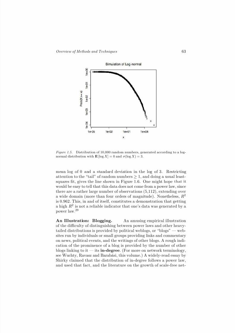
8/6/2019 Methods and Techniques of complex system science
http://slidepdf.com/reader/full/methods-and-techniques-of-complex-system-science 63/96
Overview of Methods and Techniques 63
Figure 1.5. Distribution of 10,000 random numbers, generated according to a log-normal distribution with E [logX ] = 0 and σ(logX ) = 3.
mean log of 0 and a standard deviation in the log of 3. Restricting
attention to the “tail” of random numbers ≥ 1, and doing a usual least-squares fit, gives the line shown in Figure 1.6. One might hope that itwould be easy to tell that this data does not come from a power law, sincethere are a rather large number of observations (5,112), extending overa wide domain (more than four orders of magnitude). Nonetheless, R2
is 0.962. This, in and of itself, constitutes a demonstration that gettinga high R2 is not a reliable indicator that one’s data was generated by apower law.29
An Illustration: Blogging. An amusing empirical illustrationof the difficulty of distinguishing between power laws and other heavy-tailed distributions is provided by political weblogs, or “blogs” — web-sites run by individuals or small groups providing links and commentaryon news, political events, and the writings of other blogs. A rough indi-cation of the prominence of a blog is provided by the number of otherblogs linking to it — its in-degree. (For more on network terminology,see Wuchty, Ravasz and Barabasi, this volume.) A widely-read essay byShirky claimed that the distribution of in-degree follows a power law,and used that fact, and the literature on the growth of scale-free net-
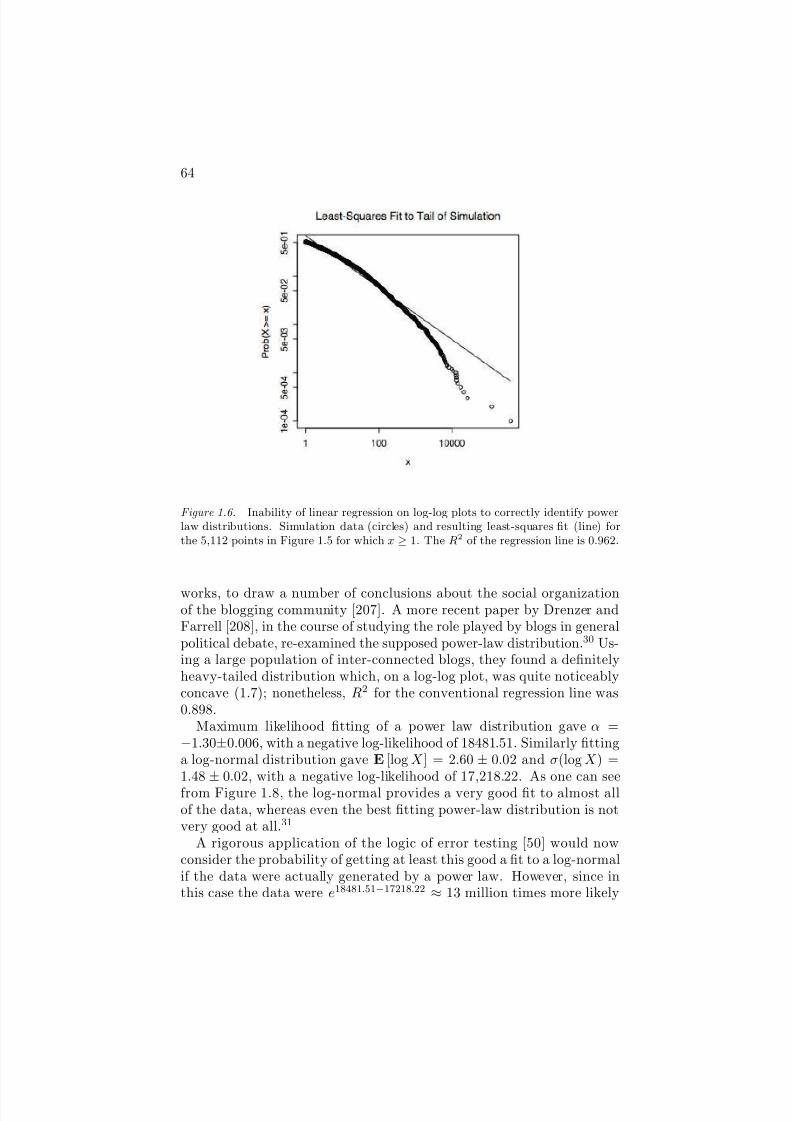
8/6/2019 Methods and Techniques of complex system science
http://slidepdf.com/reader/full/methods-and-techniques-of-complex-system-science 64/96
64
Figure 1.6. Inability of linear regression on log-log plots to correctly identify powerlaw distributions. Simulation data (circles) and resulting least-squares fit (line) forthe 5,112 points in Figure 1.5 for which x ≥ 1. The R2 of the regression line is 0.962.
works, to draw a number of conclusions about the social organizationof the blogging community [207]. A more recent paper by Drenzer andFarrell [208], in the course of studying the role played by blogs in generalpolitical debate, re-examined the supposed power-law distribution.30 Us-ing a large population of inter-connected blogs, they found a definitelyheavy-tailed distribution which, on a log-log plot, was quite noticeablyconcave (1.7); nonetheless, R2 for the conventional regression line was0.898.
Maximum likelihood fitting of a power law distribution gave α =−1.30±0.006, with a negative log-likelihood of 18481.51. Similarly fittinga log-normal distribution gave E [log X ] = 2.60 ± 0.02 and σ(log X ) =1.48
±0.02, with a negative log-likelihood of 17,218.22. As one can see
from Figure 1.8, the log-normal provides a very good fit to almost allof the data, whereas even the best fitting power-law distribution is notvery good at all.31
A rigorous application of the logic of error testing [50] would nowconsider the probability of getting at least this good a fit to a log-normalif the data were actually generated by a power law. However, since inthis case the data were e18481.51−17218.22 ≈ 13 million times more likely

8/6/2019 Methods and Techniques of complex system science
http://slidepdf.com/reader/full/methods-and-techniques-of-complex-system-science 65/96
Overview of Methods and Techniques 65
Figure 1.7. Empirical distribution of the in-degrees of political weblogs (“blogs”).Horizontal axis: number of incoming links d; vertical axis: fraction of all blogs withat least that many links, Pr(D ≥ d); both axes are on a log-log scale. Circles showthe actual distribution; the straight line is a least-squares fit to these values. Thisdoes not produce a properly normalized probability distribution but it does have anR2 of 0.898, despite the clear concavity of the curve.
under the log-normal distribution, any sane test would reject the power-law hypothesis.
8.5 Other Measures of Complexity
Considerations of space preclude an adequate discussion of furthercomplexity measures. It will have to suffice to point to some of theleading ones. The thermodynamic depth of Lloyd and Pagels [182]measures the amount of information required to specify a trajectoryleading to a final state, and is related both to departure from thermody-namic equilibrium and to retrodiction [209]. Huberman and Hogg [210],and later Wolpert and Macready [211] proposed to measure complexityas the dissimilarity between different levels of a given system, on thegrounds that self-similar structures are actually very easy to describe.(Say what one level looks like, and then add that all the rest are thesame!) Wolpert and Macready’s measure of self-dissimilarity is, in turn,closely related to a complexity measure proposed by Sporns, Tononi and
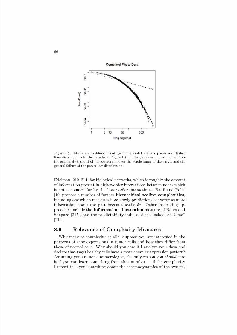
8/6/2019 Methods and Techniques of complex system science
http://slidepdf.com/reader/full/methods-and-techniques-of-complex-system-science 66/96
66
Figure 1.8. Maximum likelihood fits of log-normal (solid line) and power law (dashedline) distributions to the data from Figure 1.7 (circles); axes as in that figure. Notethe extremely tight fit of the log-normal over the whole range of the curve, and thegeneral failure of the power-law distribution.
Edelman [212–214] for biological networks, which is roughly the amountof information present in higher-order interactions between nodes whichis not accounted for by the lower-order interactions. Badii and Politi[10] propose a number of further hierarchical scaling complexities,including one which measures how slowly predictions converge as moreinformation about the past becomes available. Other interesting ap-proaches include the information fluctuation measure of Bates andShepard [215], and the predictability indices of the “school of Rome”[216].
8.6 Relevance of Complexity Measures
Why measure complexity at all? Suppose you are interested in thepatterns of gene expressions in tumor cells and how they differ fromthose of normal cells. Why should you care if I analyze your data anddeclare that (say) healthy cells have a more complex expression pattern?Assuming you are not a numerologist, the only reason you should careis if you can learn something from that number — if the complexityI report tells you something about the thermodynamics of the system,

8/6/2019 Methods and Techniques of complex system science
http://slidepdf.com/reader/full/methods-and-techniques-of-complex-system-science 67/96
Overview of Methods and Techniques 67
how it responds to fluctuations, how easy it is to control, etc. A goodcomplexity measure, in other words, is one which is relevant to manyother aspects of the system measured. A bad complexity measure lackssuch relevance; a really bad complexity measure would be positivelymisleading, lumping together things with no real connection or similarity just because they get the same score. My survey here has focused oncomplexity measures which have some claim to relevance, deliberatelyavoiding the large number of other measures which lack it [217].
9. Guide to Further Reading
9.1 General
There is no systematic or academically-detailed survey of the “pat-terns” of complex systems, but there are several sound informal discus-sions: Axelrod and Cohen [218], Flake [219], Holland [220] and Simon[221]. The book by Simon, in particular, repays careful study.
On the “topics”, the only books I can recommend are the ones by Boc-cara [222] and Flake [219]. The former emphasizes topics from physics,chemistry, population ecology and epidemiology, along with analyticalmethods, especially from nonlinear dynamics. Some sections will be eas-ier to understand if one is familiar with statistical mechanics at the levelof, e.g., [200], but this is not essential. It does not, however, describeany models of adaptation, learning, evolution, etc. Many of those topics
are covered in Flake’s book, which however is written at a much lowerlevel of mathematical sophistication.
On foundational issues about complexity, the best available surveys[10, 195] both neglect the more biological aspects of the area, and assumeadvanced knowledge of statistical mechanics on the part of their readers.
9.2 Data Mining and Statistical Learning
There are now two excellent introductions to statistical learning anddata mining, [223] and [31]. The former is more interested in computa-tional issues and the initial treatment of data; the latter gives more em-phasis to pure statistical aspects. Both are recommended unreservedly.Baldi and Brunak [95] introduces machine learning via its applicationsto bioinformatics, and so may be especially suitable for readers of thisbook.
For readers seriously interested in understanding the theoretical basisof machine learning, [224] is a good starting point. The work of Vapnik[22, 225, 226] is fundamental; the presentation in his [22] is enlivened bymany strong and idiosyncratic opinions, pungently expressed. [40] de-
8/6/2019 Methods and Techniques of complex system science
http://slidepdf.com/reader/full/methods-and-techniques-of-complex-system-science 68/96
68
scribes the very useful class of models called “support vector machines”,as well as giving an extremely clear exposition of key aspects of statisticallearning theory. Those interested in going further will find that most of the relevant literature is still in the form of journals — Machine Learning ,Journal of Machine Learning Research (free on-line at www.jmlr.org),Neural Computation — and especially annual conference proceedings —Computational Learning Theory (COLT), International Conference onMachine Learning (ICML), Uncertainty in Artificial Intelligence (UAI),Knowledge Discovery in Databases (KDD), Neural Information Process-ing Systems (NIPS), and the regional versions of them (EuroCOLT, Pa-cific KDD, etc.).
Much of what has been said about model selection could equally wellhave been said about what engineers call system identification, andin fact is said in good modern treatments of that area, of which [227]may be particularly recommended.
In many respects, data mining is an extension of exploratory dataanalysis; the classic work by Tukey [228] is still worth reading. Nodiscussion of drawing inferences from data would be complete withoutmentioning the beautiful books by Tufte [229–231].
9.3 Time Series
Perhaps the best all-around references for the nonlinear dynamics ap-proach are [69] and [232]. The former, in particular, succeeds in in-
tegrating standard principles of statistical inference into the nonlineardynamics method. [73], while less advanced than those two b ooks, is amodel of clarity, and contains an integrated primer on chaotic dynamicsbesides. Ruelle’s little book [162] is much more subtle than it looks,full of deep insights. The SFI proceedings volumes [233, 234] are veryworthwhile. The journals Physica D, Physical Review E and Chaos oftenhave new developments.
From the statistical wing, one of the best recent textbooks is [55];there are many, many others. That by Durbin and Koopman [60] isparticularly strong on the state-space point of view. The one by [235]Azencott and Dacunha-Castelle is admirably clear on both the aims of time series analysis, and the statistical theory underlying classical meth-ods; unfortunately it typography is less easy to read than it should be.[236] provides a comprehensive and up-to-date view of the statistical the-ory for modern models, including strongly non-linear and non-Gaussianmodels. While many of the results are directly useful in application, theproofs rely on advanced theoretical statistics, in particular the geometricapproach pioneered by the Japanese school of Amari et al. [237], This

8/6/2019 Methods and Techniques of complex system science
http://slidepdf.com/reader/full/methods-and-techniques-of-complex-system-science 69/96
Overview of Methods and Techniques 69
information geometry has itself been applied by Ay to the study of complex systems [238, 239].
At the interface between the statistical and the dynamical points of view, there is an interesting conference proceedings [240] and a usefulbook by Tong [241]. Pearson’s book [242] on discrete-time models isvery good on many important issues related to model selection, andexemplifies the habit of control theorists of cheerful stealing whateverseems helpful.
Filtering. Linear filters are well-described by many textbooks incontrol theory (e.g. [243]), signal processing, time series analysis (e.g.
[55]) and stochastic dynamics (e.g. [58]).[89] provides a readable introduction to optimal nonlinear estimation,draws interesting analogies to non-equilibrium statistical mechanics andturbulence, and describes a reasonable approximation scheme. [90] is anup-to-date textbook, covering both linear and nonlinear methods, andincluding a concise exposition of the essential parts of stochastic calculus.The website run by R. W. R. Darling, www.nonlinearfiltering.webhop.net ,provides a good overview and extensive pointers to the literature.
Symbolic Dynamics and Hidden Markov Models. On sym-bolic dynamics, formal languages and hidden Markov models generally,see [10]. [198] is a good first course on formal languages and automata
theory. Charniak is a very readable introduction to grammatical infer-ence. [244] is an advanced treatment of symbolic dynamics emphasizingapplications; by contrast, [116] focuses on algebraic, pure-mathematicalaspects of the subject. [163] is good on the stochastic properties of symbolic-dynamical representations. Gershenfeld [245] gives a good mo-tivating discussion of hidden Markov models, as does Baldi and Brunak[95], while [94] describes advanced methods related to statistical sig-nal processing. Open-source code for reconstructing causal-state modelsfrom state is available from http://bactra.org/CSSR .
9.4 Cellular Automata
General. There is unfortunately no completely satisfactory unifiedtreatment of cellular automata above the recreational. Ilachinski [246]attempts a general survey aimed at readers in the physical sciences, andis fairly satisfactory on purely mathematical aspects, but is more out of date than its year of publication suggests. Chopard and Droz [247] hasgood material on models of pattern formation missing from Ilachinski,but the English is often choppy. Toffoli and Margolus [248] is inspiringand sound, though cast on a piece of hardware and a programming
8/6/2019 Methods and Techniques of complex system science
http://slidepdf.com/reader/full/methods-and-techniques-of-complex-system-science 70/96
70
environment which are sadly no longer supported. Much useful materialon CA modeling has appeared in conference proceedings [249–251].
CA as Self-Reproducing Machines. The evolution of CA beginsin [252], continues in [253], and is brought up to the modern era in [254];the last is a beautiful, thought-provoking and modest book, sadly out of print. The modern era itself opens with [255].
Mathematical and Automata-Theoretic Aspects. Many of thepapers in [256] are interesting. Ilachinski [246], as mentioned, providesa good survey. The Gutowitz volume [250] has good material on thistopic, too. [257] is up-to-date.
Lattice gases. [124] is a good introduction, [258] somewhat moreadvanced. The pair of proceedings edited by Doolen [259, 260] describemany interesting applications, and contain useful survey and pedagogicalarticles. (There is little overlap between the two volumes.)
9.5 Agent-Based Modeling
There do not seem to be any useful textbooks or monographs onagent-based modeling. The Artificial Life conference proceedings, start-ing with [255], were a prime source of inspiration for agent-based mod-eling, along with the work of Axelrod [261]. [262] is also worth reading.
The journal Artificial Life continues to be relevant, along with the From Animals to Animats conference series. Epstein and Axtell’s book [263]is in many ways the flagship of the “minimalist” approach to ABMs;while the arguments in its favor (e.g., [264, 265]) are often framed interms of social science, many apply with equal force to biology32. [266]illustrates how ABMs can be combined with extensive real-world data.Other notable publications on agent-based models include [267], span-ning social science and evolutionary biology; [268] on agent-based modelsof morphogenesis; and [269] on biological self-organization.
[131] introduces object-oriented programming and the popular Javaprogramming language at the same time; it also discusses the roots of object-orientation in computer simulation. There are many, many other
books on object-oriented programming.
9.6 Evaluating Models of Complex Systems
Honerkamp [58] is great, but curiously almost unknown. Gershenfeld[245] is an extraordinary readable encyclopedia of applied mathematics,
8/6/2019 Methods and Techniques of complex system science
http://slidepdf.com/reader/full/methods-and-techniques-of-complex-system-science 71/96
Overview of Methods and Techniques 71
especially methods which can be used on real data. Gardiner [270] isalso useful.
Monte Carlo. The old book by Hammersley and Handscomb [140]is concise, clear, and has no particular prerequisites beyond a workingknowledge of calculus and probability. [271] and [272] are both good in-troductions for readers with some grasp of statistical mechanics. Thereare also very nice discussions in [58, 31, 142]. Beckerman [143] makesMonte Carlo methods the starting point for a fascinating and highly un-conventional exploration of statistical mechanics, Markov random fields,synchronization and cooperative computation in neural and perceptual
systems.
Experimental design. Bypass the cookbook texts on standarddesigns, and consult Atkinson and Donev [155] directly.
Ecological inference. [273] is at once a good introduction, andthe source of important and practical new methods.
9.7 Information Theory
Information theory appeared in essentially its modern form with Shan-non’s classic paper [274], though there had been predecessors in bothcommunications [275] and statistics, notably Fisher (see Kullback [159]
for an exposition of these notions), and similar ideas were developed byWiener and von Neumann, more or less independently of Shannon [56].Cover and Thomas [158] is, deservedly, the standard modern textbookand reference; it is highly suitable as an introduction, and handles al-most every question most users will, in practice, want to ask. [276] isa more mathematically rigorous treatment, now free on-line. On neuralinformation theory, [172] is seminal, well-written, still very valuable, andlargely self-contained. On the relationship between physics and informa-tion, the best reference is still the volume edited by Zurek [12], and thethought-provoking paper by Margolus.
9.8 Complexity Measures
The best available survey of complexity measures is that by Badiiand Politi [10]; the volume edited by Peliti and Vulpiani [277], whiledated, is still valuable. Edmonds [278] is an online bibliography, fairlycomprehensive through 1997. [195] has an extensive literature review.
On Kolmogorov complexity, see Li and Vitanyi [177]. While the ideaof measuring complexity by the length of descriptions is usually cred-

8/6/2019 Methods and Techniques of complex system science
http://slidepdf.com/reader/full/methods-and-techniques-of-complex-system-science 72/96
72
ited to the trio of Kolmogorov, Solomonoff and Chaitin, it is implicitin von Neumann’s 1949 lectures on the “Theory and Organization of Complicated Automata” [252, Part I, especially pp. 42–56].
On MDL, see Rissanen’s book [185], and Grunwald’s lecture notes[279]. Vapnik [22] argues that when MDL converges on the optimalmodel, SRM will too, but he assumes independent data.
On statistical complexity and causal states, see [195] for a self-containedtreatment, and [188] for extensions of the theory.
Acknowledgments
This work has been supported by a grant from the James S. McDon-
nell Foundation, and was finished while enjoying the hospitality of theInstitut des Systemes Complexes, the Laboratoire de l’Informatique duParalleisme and the Exystence Thematic Institute on Discrete and Com-putational Aspects of Complex Systems at the Ecole Normale Superierede Lyon. I am grateful to Michel Morvan and Cris Moore, organiz-ers of the “Science et Gastronomie 2003” workshop, for allowing me topresent some of this material there, and to my fellow participants fortheir critical comments. It is a pleasure to acknowledge discussions withDave Albers, Satinder Singh Baveja, Philippe Binder, Sven Bruckener,Sandra Chapman, Markus Christen, Michael Cohen, Jim Crutchfield,Gunther Eble, Dave Feldman, Walter Fontana, Peter Grassberger, RobHaslinger, John Holland, Herbert Jaeger, Jurgen Jost, Michael Lach-
mann, Alex Lancaster, Norm Margolus, Cris Moore, Mark Newman,Scott Page, Mitchell Porter, Kristina Shalizi, Carl Simon, Eric Smith,Ricard Sole, Bill Tozier, Erik van Nimwegen and Nick Watkins. Specialthanks to Prof. Cohen for permission to take a triangle he drew andadd a corner to it; to Profs. Drenzer and Farrell for permission to usetheir data on weblogs; to Bill Tozier for suggesting that the leitmotifs of complex systems are analysis patterns, and for advice on agents; to KaraKedi for daily validation of von Neumann’s remarks on the complexityof cats; to Mathew Dafilis and Nigel Phillips for spotting misprints; toKristina Shalizi for assistance on linear models of time series and forcareful reading of a draft; and to Kristina and Rob for resisting the ideathat there is such a thing as complex systems science. Finally, I wish toacknowledge the patience of the editors.
Notes1. Several books pretend to give a unified presentation of the topics. To date, the only
one worth reading is [222], which however omits all models of adaptive systems.
2. Not all data mining is strictly for predictive models. One can also mine for purely de-scriptive models, which try to, say, cluster the data points so that more similar ones are closer

8/6/2019 Methods and Techniques of complex system science
http://slidepdf.com/reader/full/methods-and-techniques-of-complex-system-science 73/96
Overview of Methods and Techniques 73
together, or just assign an over-all likelihood score. These, too, can be regarded as minimiz-ing a cost function (e.g., the dis-similarity within clusters plus the similarity across clusters).The important point is that good descriptions, in this sense, are implicitly predictive, eitherabout other aspects of the data or about further data from the same source.
3. A subtle issue can arise here, in that not all errors need be equally bad for us. Inscientific applications, we normally aim at accuracy as such, and so all errors are equally bad.But in other applications, we might care very much about otherwise small inaccuracies insome circumstances, and shrug off large inaccuracies in others. A well-designed loss functionwill represent these desires. This does not change the basic principles of learning, but it canmatter a great deal for the final machine [280].
4. Here and throughout, I try to follow the standard notation of probability theory, socapital letters (X, Y , etc.) denote random variables, and lower-case ones particular values orrealizations — so X = the role of a die, whereas x = 5 (say).
5. This is called the convergence i n probability of L(θ) to its mean value. For apractical introduction to such convergence properties, the necessary and sufficient conditions
for them to obtain, and some thoughts about what one can do, statistically, when they donot, see [51].
6. The precise definition of the VC dimension is somewhat involved, and omitted herefor brevity’s sake. See [224, 40] for clear discussions.
7. For instance, one can apply the independent-sample theory to learning feedback controlsystems [281].
8. Actually, the principle goes back to Aristotle at least, and while Occam used it often,he never used exactly those words [282, translator’s introduction].
9. This is very close to the notion of the power of a statistical hypothesis test [283], andalmost exactly the same as the severity of such a test [50].
10. One could, of course, build a filter which uses later y values as well; this is a non-
causal or smoothing filter. This is clearly not suitable for estimating the state in real time,but often gives more accurate estimates when it is applicable. The discussion in the textgenerally applies to smoothing filters, at some cost in extra notation.
11. Equivalent terms are future-resolving or right-resolving (from nonlinear dynamics)and deterministic (the highly confusing contribution of automata theory).
12. Early publications on this work started with the assumption that the discrete valueswere obtained by dividing continuous measurements into bins of width ǫ, and so called theresulting models “ǫ-machines”. This name is unfortunate: that is usually a bad way of discretizing data (§1.3.6.4), the quantity ǫ plays no role in the actual theory, and the nameis more than usually impenetrable to outsiders. While I have used it extensively myself, itshould probably be avoided.
13. An alternate definition [10] lo oks at the entropy rate (§1.7) of the symbol sequences: agenerating partition is one which maximizes the entropy rate, which is the same as maximizingthe extra information about the initial condition x provided by each symbol of the sequenceΦ(x).
14.Quantum versions of CA are an active topic of investigation, but unlikely to be of biological relevance [246].
15. In a talk at the Santa Fe Institute, summer of 2000; the formula does not seem to havebeen published.
16. A simple argument just invokes the central limit theorem. The number of points falling
within the shaded region has a binomial distribution, with success parameter p, so asymp-totically x/n has a Gaussian distribution with mean p and standard deviation
p(1 − p)/n.
A non-asymptotic result comes from Chernoff’s inequality [281], which tells us that, for all
n, Pr(|x/n− p| ≥ ǫ) < 2e−2nǫ2
.
17. The chain needs to be irreducible, meaning one can go from any point to any otherpoint, and positive recurrent, meaning that there’s a positive probability of returning to anypoint infinitely often.
18. Unless our choices for the transition probabilities are fairly perverse, the central limittheorem still holds, so asymptotically our estimate still has a Gaussian distribution around
8/6/2019 Methods and Techniques of complex system science
http://slidepdf.com/reader/full/methods-and-techniques-of-complex-system-science 74/96
74
the true value, and still converges as N −1/2 for large enough N , but determining what’s“large enough” is trickier.
19. An important exception is the case of equilibrium statistical mechanics, where thedynamics under the Metropolis algorithm are like the real dynamics.
20. For a p edagogical discussion, with examples, of how compression algorithms may bemisused, see http://bactra.org/notebooks/cep-gzip.html.
21.The issue of what language to write the program in is secondary; writing a programto convert from one language to another just adds on a constant to the length of the over-allprogram, and we will shortly see why additive constants are not important here.
22. Very short programs can calculate π to arbitrary accuracy, and the length of theseprograms does not grow as the number of digits calculated does. So one could run one of these programs until it had produced the first two quadrillion digits, and then erase the firsthalf of the output, and stop.
23. [167] is perhaps the most notorious; see [168] and especially [169] for critiques.
24.It is certainly legitimate to regard any dynamical process as also a computational
process, [284–286, 195], so one could argue that the data is produced by some kind of program.But even so, this computational process generally does not resemble that of the minimal,Kolmogorov program at all.
25. It is important to note [185, chapter 3] that if we allowed any possible model in Θ, findthe minimum would, once again, be incomputable. This restriction to a definite, perhapshierarchically organized, class of models is vitally important.
26. Take our favorite class of models, and add on deterministic models which produceparticular fixed blocks of data with probability 1. For any of these models θ, L(x, θ) is either0 (if x is what that model happens to generate) or ∞. Then, once we have our data, andfind a θ which generates that and nothing but that, re-arrange the coding scheme so thatD(θ,Θ) = 1; this is always possible. Thus, C SC(x,Θ) = 1 bit.
27. This does not contradict the convergence result of the last paragraph; one of the not-too-onerous conditions mentioned in the previous paragraph is that the coding scheme remainfixed, and we’re violating that.
28. Technically, a given regular language (§1.3.6).
29. If I replace the random data by the exact log-normal probability distribution over thesame range, and do a least-squares fit to that, the R2 actually increases, to 0.994.
30. Profs. Drenzer and Farrell kindly shared their data with me, but the figures and analysisthat follow are my own.
31.Note that the log-normal curve fitted to the whole data continues to match the datawell even in the tail. For further discussion, omitted here for reasons of space, seehttp://bactra.org/weblog/232.html.
32. In reading this literature, it may be helpful to bear in mind that by “methodologicalindividualism”, social scientists mean roughly what biologists do by “reductionism”.
References
[1] Erich Gamma, Richard Helm, Ralph Johnson, and John Vlissides.Design Patterns: Elements of Reusable Object-Oriented Software.
Addison-Wesley, Reading, Massachusetts, 1995.[2] Russell W. Anderson. Random-walk learning: A neurobiological
correlate to trial-and-error. In O. M. Omidvar and J. Dayhoff,editors, Progress in Neural Networks, pages 221–244. AcademicPress, Boston, 1988.
[3] S. Mueller, J. Marchettod, S. Airaghi, and P. Koumoutsakos. Op-timization based on bacterial chemotaxis. IEEE Transactions on
8/6/2019 Methods and Techniques of complex system science
http://slidepdf.com/reader/full/methods-and-techniques-of-complex-system-science 75/96
Overview of Methods and Techniques 75
Evolutionary Computation , 6:16–29, 2002.
[4] Herbert A. Simon. The architecture of complexity: Hierarchic sys-tems. Proceedings of the American Philosophical Society , 106:467–482, 1962. Reprinted as chapter 8 of [221].
[5] Herbert A. Simon. On a class of skew distribution functions.Biometrika , 42:425–440, 1955.
[6] Alan Turing. The chemical basis of morphogenesis. Philosophical Transactions of the Royal Society B , 237:37–72, 1952.
[7] S. P. Strong, B. Freedman, William Bialek, andR. Koberle. Adaptation and optimal chemotactic strat-
egy for e. coli . Physical Review E , 57:4604–4617, 1998.http://arxiv.org/abs/adap-org/9706001 .
[8] U. Alon, M. G. Surette, N. Barkai, and S. Leibler. Robustness inbacterial chemotaxis. Nature, 397:168–171, 1999.
[9] Tau-Mu Yi, Yun Huang, Melvin I. Simon, and John Doyle. Robustperfect adaptation in bacterial chemotaxis through integral feed-back control. Proceedings of the National Academy of Sciences,97:4649–4653, 2000.
[10] Remo Badii and Antonio Politi. Complexity: Hierarchical Struc-tures and Scaling in Physics. Cambridge University Press, Cam-bridge, 1997.
[11] Walter Fontana and Leo W. Buss. “The Arrival of the Fitest”: Towards a theory of biological organiza-tion. Bulletin of Mathematical Biology , 56:1–64, 1994.http://www.santafe.edu/∼walter/Papers/arrival.US.ps.gz.
[12] Wojciech H. Zurek, editor. Complexity, Entropy, and the Physicsof Information , Reading, Massachusetts, 1990. Addison-Wesley.
[13] Uriel Frisch. Turbulence: The Legacy of A. N. Kolmogorov . Cam-bridge University Press, Cambridge, England, 1995.
[14] Mark C. Cross and Pierre Hohenberg. Pattern formation out of equilibrium. Reviews of Modern Physics, 65:851–1112, 1993.
[15] Philip Ball. The Self-Made Tapestry: Pattern Formation in Nature.Oxford University Press, Oxford, 1999.
[16] John H. Holland. Adaptation in Natural and Artificial Systems:An Introductory Analysis with Applications to Biology, Control,and Artificial Intelligence. MIT Press, Cambridge, Massachusetts,2nd edition, 1992. First edition, Ann Arbor, Michigan: Universityof Michigan Press, 1975.
8/6/2019 Methods and Techniques of complex system science
http://slidepdf.com/reader/full/methods-and-techniques-of-complex-system-science 76/96
76
[17] Melanie Mitchell. An Introduction to Genetic Algorithms. MITPress, Cambridge, Massachusetts, 1996.
[18] Herbert Gintis. Game Theory Evolving: A Problem-Centered In-troduction to Modeling Strategic Interaction . Princeton UniversityPress, Princeton, 2000.
[19] Josef Hofbauer and Karl Sigmund. The Theory of Evolution and Dynamical Systems: Mathematical Aspects of Selection . Cam-bridge University Press, Cambridge, England, 1988.
[20] K. H. Fischer and J. A. Hertz. Spin Glasses. Cambridge Studiesin Magnetism. Cambridge University Press, Cambridge, 1988.
[21] Daniel L. Stein. Spin glasses: Still complex after all these years?In T. Elze, editor, Quantum Decoherence and Entropy in Complex Systems, Berlin, 2003. Springer-Verlag.
[22] Vladimir N. Vapnik. The Nature of Statistical Learning Theory .Springer-Verlag, Berlin, 2nd edition, 2000.
[23] Hirotugu Akaike. Information theory and an extension of the max-imum likelihood principle. In B. N. Petrov and F. Caski, editors,Proceedings of the Scond International Symposium on Informa-tion Theory , pages 267–281, Budapest, 1973. Akademiai Kiado.Reprinted in [287, pp. 199–213].
[24] Hirotugu Akaike. On entropy maximization principle. In P. R.
Krishnaiah, editor, Applications of Statistics, pages 27–41, Ams-terdam, 1977. North-Holland.
[25] G. Schwarz. Estimating the dimension of a model. The Annals of Statistics, 6:461–464, 1978.
[26] Sara van de Geer. Empirical Processes in M-Estimation . Cam-bridge University Press, Cambridge, England, 2000.
[27] Earl Derr Biggers. Behind That Curtain . Grosset and Dunlap,New York, 1928.
[28] Leslie G. Valiant. A theory of the learnable. Communications of the Association for Computing Machinery , 27:1134–1142, 1984.
[29] Xuhui Shao, Vladimir Cherkassky, and William Li. Measuring
the VC-dimension using optimized experimental design. Neural Computation , 12:1969–1986, 2000.
[30] Ron Meir. Nonparametric time series prediction through adaptivemodel selection. Machine Learning , 39:5–34, 2000.
[31] Trevor Hastie, Robert Tibshirani, and Jerome Friedman. The El-ements of Statistical Learning: Data Mining, Inference, and Pre-diction . Springer-Verlag, New York, 2001.
8/6/2019 Methods and Techniques of complex system science
http://slidepdf.com/reader/full/methods-and-techniques-of-complex-system-science 77/96
Overview of Methods and Techniques 77
[32] Brian D. Ripley. Pattern Recognition and Neural Networks. Cam-bridge University Press, Cambridge, England, 1996.
[33] Grace Wahba. Spline Models for Observational Data . Society forIndustrial and Applied Mathematics, Philadelphia, 1990.
[34] Martin Anthony and Peter L. Bartlett. Neural Network Learning:Theoretical Foundations. Cambridge University Press, Cambridge,England, 1999.
[35] Achilleas Zapranis and Apostolos-Paul Refenes. Principles of Neu-ral Model Identification, Selection and Adequacy: With Applica-tions to Financial Econometrics. Springer-Verlag, London, 1999.
[36] A. Engel and C. Van den Broeck. Statistical Mechanics of Learn-ing . Cambridge University Press, Cambridge, England, 2001.
[37] Leo Breiman, Jerome Friedman, R. Olshen, and C. Stone. Clas-sification and Regression Trees. Wadsworth, Belmont, California,1984.
[38] Gerd Gigerenzer, Peter M. Todd, and the ABC Research Group.Simple Heuristics That Make Us Smart . Oxford University Press,Oxford, 1999.
[39] Ralf Herbrich. Learning Kernel Classifiers: Theory and Algo-rithms. MIT Press, Cambridge, Massachusetts, 2002.
[40] Nello Cristianini and John Shawe-Taylor. An Introduction to Sup-port Vector Machines: And Other Kernel-Based Learning Methods.
Cambridge University Press, Cambridge, England, 2000.[41] Judea Pearl. Causality: Models, Reasoning, and Inference. Cam-
bridge University Press, Cambridge, England, 2000.
[42] Glenn Shafer. The Art of Causal Conjecture. MIT Press, Cam-bridge, Massachusetts, 1996.
[43] Peter Spirtes, Clark Glymour, and Richard Scheines. Causation,Prediction, and Search . MIT Press, Cambridge, Massachusetts,2nd edition, 2001.
[44] Peter Dayan, Geoffrey E. Hinton, Radford M.Neal, and Richard S. Zemel. The Helmholtzmachine. Neural Computation , 7:889–904, 1995.
http://www.cs.utoronto.ca/∼hinton/absps/helmholtz.htm.[45] Pedro Domingos. The role of Occam’s Razor in knowledge dis-
covery. Data Mining and Knowledge Discovery , 3:409–425, 1999.http://www.cs.washington.edu/home/pedrod/dmkd99.pz.gz .
[46] Judy L. Klein. Statistical Visions in Time: A History of TimeSeries Analysis, 1662–1938 . Cambridge University Press, Cam-bridge, England, 1997.
8/6/2019 Methods and Techniques of complex system science
http://slidepdf.com/reader/full/methods-and-techniques-of-complex-system-science 78/96
78
[47] P. A. M. Dirac. Principles of Quantum Mechanics. ClarendonPress, Oxford, 1935.
[48] Frank B. Knight. A predictive view of continuous time processes.The Annals of Probability , 3:573–596, 1975.
[49] Frank B. Knight. Foundations of the Prediction Process, volume 1of Oxford Studies in Probability . Clarendon Press, Oxford, 1992.
[50] Deborah G. Mayo. Error and the Growth of Experimental Knowl-edge. University of Chicago Press, Chicago, 1996.
[51] Robert M. Gray. Probability, Random Processes, and Ergodic Properties. Springer-Verlag, New York, 1988.http://ee-www.stanford.edu/
∼gray/arp.html.
[52] Ishwar V. Basawa and David John Scott. Asymptotic Optimal Inference for Non-Ergodic Models. Springer-Verlag, Berlin, 1983.
[53] Bruce J. West and Bill Deering. The Lure of Modern Science:Fractal Thinking . World Scientific, Singapore, 1995.
[54] William H. Press, Saul A. Teukolsky, William T. Vetterling, andBrian P. Flannery. Numerical Recipes in C: The Art of ScientificComputing . Cambridge University Press, Cambridge, England,2nd edition, 1992.
[55] Robert H. Shumway and David S. Stoffer. Time Series Analysisand Its Applications. Springer Texts in Statistics. Springer-Verlag,New York, 2000.
[56] Norbert Wiener. Cybernetics: Or, Control and Communication in the Animal and the Machine. MIT Press, Cambridge, Mas-sachusetts, 2nd edition, 1961. First edition New York: Wiley, 1948.
[57] Barbara B. Hubbard. The World According to Wavelets: The story of a mathematical technique in the making . A. K. Peters, Wellesley,Massachusetts, 1996.
[58] Josef Honerkamp. Stochastic Dynamical Systems: Concepts, Nu-merical Methods, Data Analysis. VCH, New York, 1994. Trans-lated by Katja Lindenberg.
[59] G. E. P. Box and G. M. Jenkins. Time Series Analysis, Forecasting,and Control . Holden-Day, Oakland, California, 1970.
[60] James Durbin and Siem Jam Koopman. Time Series Analysis by State Space Methods. Oxford University Press, Oxford, 2001.
[61] Gregory L. Eyink. Linear stochastic models of nonlinear dynamicalsystems. Physical Review E , 58:6975–6991, 1998.
[62] O. E. Barndorff-Nielsen, J. L. Jensen, and M. Sorensen. Parametricmodelling of turbulence. Philosophical Transactions of the Royal Society A, 332:439–455, 1990.
8/6/2019 Methods and Techniques of complex system science
http://slidepdf.com/reader/full/methods-and-techniques-of-complex-system-science 79/96
Overview of Methods and Techniques 79
[63] Gregory L. Eyink and Francis J. Alexander. Predictive turbulencemodeling by variational closure. Journal of Statistical Physics,91:221–283, 1998.
[64] Jan Beran. Statistics for Long-Memory Processes. Chapman andHall, New York, 1994.
[65] Paul Embrechts and Makoto Maejima. Selfsimilar processes.Princeton University Press, Princeton, New Jersey, 2002.
[66] Denis Bosq. Nonparametric Statistics for Stochastic Processes:Estimation and Prediction . Springer-Verlag, Berlin, 2nd edition,1998.
[67] Paul Algoet. Universal schemes for prediction, gambling andportfolio selection. The Annals of Probability , 20:901–941, 1992.See also an important Correction, The Annals of Probability , 23(1995): 474–478.
[68] Floris Takens. Detecting strange attractors in fluid turbulence. InD. A. Rand and L. S. Young, editors, Symposium on Dynamical Systems and Turbulence, pages 366–381, Berlin, 1981. Springer-Verlag.
[69] Holger Kantz and Thomas Schreiber. Nonlinear Time Series Anal-ysis. Cambridge University Press, Cambridge, England, 1997.
[70] Kevin Judd and Alistair Mees. Embedding as a modeling problem.
Physica D, 120:273–286, 1998.
[71] Michael Small and C. K. Tse. Optimal embedding parame-ters: A modelling paradigm. Physica D, 194:283–296, 2004.http://arxiv.org/abs/physics/0308114 .
[72] Matthew B. Kennel, R. Brown, and Henry D. I. Abarbanel. De-termining minimum embedding dimension using a geometric con-struction. Physical Review A, 45:3403–3411, 1992.
[73] Julien Clinton Sprott. Chaos and Time-Series Analysis. OxfordUniversity Press, Oxford, 2003.
[74] L. A. Smith. Intrinsic limits on dimension calculations. Physics
Letters A, 133:283–288, 1988.[75] Andrew M. Fraser and Harry L. Swinney. Independent coordinates
for strange attractors from mutual information. Physical Review A, 33:1134–1140, 1986.
[76] Christopher J. Cellucci, Alfonso M. Albano, and P. E. Rapp.Comparative study of embedding methods. Physical Review E ,67:062210, 2003.
8/6/2019 Methods and Techniques of complex system science
http://slidepdf.com/reader/full/methods-and-techniques-of-complex-system-science 80/96
80
[77] Christophe Letellier and Luis A. Aguirre. Investigating nonlineardynamics from time series: The influence of symmetries and thechoice of observables. Chaos, 12:549–558, 2002.
[78] Norbert Wiener. Extrapolation, Interpolation, and Smoothing of Stationary Time Series: With Engineering Applications. The Tech-nology Press of the Massachusetts Institute of Technology, Cam-bridge, Massachusetts, 1949.
[79] Andrei N. Kolmogorov. Interpolation und extrapolation von sta-tionaren zufalligen folgen. Bulletin of the Academy Sciences,USSR, Math., 3:3–14, 1941. In Russian with German summary.
[80] R. E. Kalman. A new approach to linear filtering and predic-
tion problems. ASME Transactions, Journal of Basic Engineering ,82D:35–50, 1960.
[81] R. E. Kalman and R. S. Bucy. New results in linear filtering andprediction. ASME Transactions, Journal of Basic Engineering ,83D:95–108, 1961.
[82] Richard S. Bucy. Lectures on Discrete Time Filtering . Springer-Verlag, Berlin, 1994.
[83] R. L. Stratonovich. Conditional Markov Processes and Their Ap-plication to the Theory of Optimal Control . American Elsevier,New York, second edition, 1968. Translated by R. N. and N. B.McDonough. Preface by Richard Bellman. Revised by the author.
First edition, Uslovnyye markovskiye protessy i ikh primeneiyek teorri optimal’nogo upravleniya , Msocow: Moscow UniversityPress, 1966.
[84] Harold J. Kushner. Dynamical equations for optimal nonlinearfiltering. Journal of Differential Equations, 3:179–190, 1967.
[85] Robert S. Lipster and Albert N. Shiryaev. Statistics of Random Processes. Springer-Verlag, Berlin, second edition, 2001. Two vol-umes. Trans. A. B. Aries. First English edition 1977–1978. Firstpublished as Statistika slucha inykh protessov , Moscow: Nauka,1974.
[86] Hisashi Tanizaki. Nonlinear Filters: Estimation and Applications.
Springer-Verlag, Berlin, second edition, 1996.[87] R. W. R. Darling. Geometrically intrinsic nonlinear recur-
sive filters I: Algorithms. Technical Report 494, Statis-tics Department, University of California-Berkeley, 1998.http://www.stat.berkeley.edu/tech-reports/494.abstract .
[88] R. W. R. Darling. Geometrically intrinsic nonlinear re-cursive filters II: Foundations. Technical Report 512,
8/6/2019 Methods and Techniques of complex system science
http://slidepdf.com/reader/full/methods-and-techniques-of-complex-system-science 81/96
Overview of Methods and Techniques 81
Statistics Department, University of California-Berkeley, 1998.http://www.stat.berkeley.edu/tech-reports/512.abstract .
[89] Gregory L. Eyink. A variational formulation of optimal nonlinearestimation. Methodology and Computing in Applied Probability ,submitted, 2000. http://arxiv.org/abs/physics/0011049 .
[90] N. U. Ahmed. Linear and Nonlinear Filtering for Scientists and Engineers. World Scientific, Singapore, 1998.
[91] Noam Chomsky. Three models for the description of language.IRE Transactions on Information Theory , 2:113–124, 1956.
[92] Eugene Charniak. Statistical Language Learning . MIT Press, Cam-
bridge, Massachusetts, 1993.[93] Christopher D. Manning and Hinrich Schutze. Foundations of Sta-
tistical Natural Language Processing . MIT Press, Cambridge, Mas-sachusetts, 1999.
[94] Robert J. Elliott, Lakhdar Aggoun, and John B. Moore. Hidden Markov Models: Estimation and Control , volume 29 of Applica-tions of Mathematics: Stochastic Modelling and Applied Probabil-ity . Springer-Verlag, New York, 1995.
[95] Pierre Baldi and Søren Brunak. Bioinformatics: The MachineLearning Approach . MIT Press, Cambridge, Massachusetts, secondedition, 2001.
[96] Radford M. Neal and Geoffrey E. Hinton. A view of the EMalgorithm that justifies incremental, sparse, and other variants. InJordan [144], pages 355–368.
[97] Jorma Rissanen. A universal data compression system. IEEE Transactions on Information Theory , 29:656–664, 1983.
[98] Frans Willems, Yuri Shtarkov, and Tjalling Tjalkens. The context-tree weighting method: Basic properties. IEEE Transactions on Information Theory , 41:653–664, 1995.
[99] Dana Ron, Yoram Singer, and Naftali Tishby. The power of amne-sia: Learning probabilistic automata with variable memory length.Machine Learning , 25:117–149, 1996.
[100] Peter Buhlmann and Abraham J. Wyner. Variable lengthMarkov chains. The Annals of Statistics, 27:480–513, 1999.http://www.stat.berkeley.edu/tech-reports/479.abstract1 .
[101] Matthew B. Kennel and Alistair I. Mees. Context-tree modeling of observed symbolic dynamics. Physical Review E , 66:056209, 2002.
[102] James P. Crutchfield and Karl Young. Inferring statistical com-plexity. Physical Review Letters, 63:105–108, 1989.

8/6/2019 Methods and Techniques of complex system science
http://slidepdf.com/reader/full/methods-and-techniques-of-complex-system-science 82/96
82
[103] Herbert Jaeger. Observable operator models for discretestochastic time series. Neural Computation , 12:1371–1398,2000. http://www.faculty.iu-bremen.de/hjaeger/pubs/
oom neco00.pdf.
[104] Michael L. Littman, Richard S. Sutton, and Satinder Singh.Predictive representations of state. In Thomas G. Di-etterich, Suzanna Becker, and Zoubin Ghahramani, edi-tors, Advances in Neural Information Processing Systems 14,pages 1555–1561, Cambridge, Massachusetts, 2002. MIT Press.http://www.eecs.umich.edu/∼baveja/Papers/psr.pdf.
[105] Cosma Rohilla Shalizi and Kristina Lisa Shalizi. Blind con-
struction of optimal nonlinear recursive predictors for discrete se-quences. In Max Chickering and Joseph Halpern, editors, Uncer-tainty in Artificial Intelligence: Proceedings of the Twentieth Con- ference, pages 504–511, Arlington, Virginia, 2004. AUAI Press.http://arxiv.org/abs/cs.LG/0406011 .
[106] Wesley C. Salmon. Statistical Explanation and Statistical Rele-vance. University of Pittsburgh Press, Pittsburgh, 1971. Withcontributions by Richard C. Jeffrey and James G. Greeno.
[107] Wesley C. Salmon. Scientific Explanation and the Causal Structureof the World . Princeton University Press, Princeton, 1984.
[108] Satinder Singh, Michael L. Littman, Nicholas K. Jong, David
Pardoe, and Peter Stone. Learning predictive state rep-resentations. In Tom Fawcett and Nina Mishra, edi-tors, Proceedings of the Twentieth International Conferenceon Machine Learning (ICML-2003), pages 712–719. AAAIPress, 2003. http://www.eecs.umich.edu/∼baveja/Papers/
ICMLfinal.ps.gz.
[109] Daniel R. Upper. Theory and Algorithms for Hidden Markov Models and Generalized Hidden Markov Mod-els. PhD thesis, University of California, Berkeley,1997. http://www.santafe.edu/projects/CompMech/
papers/TAHMMGHMM.html .
[110] P. Dupont, F. Denis, and Y. Esp osito. Links b e-
tween probabilistic automata and hidden Markov mod-els: Probability distributions, learning models and induc-tion algorithms. Pattern Recognition , forthcoming, 2004.http://www.info.ucl.ac.be/people/pdupont/pdupont/
postscript/Links PA HMM preprint.ps.gz.
[111] Herbert Jaeger. Characterizing distributions of stochas-tic processes by linear operators. Technical Report 62,

8/6/2019 Methods and Techniques of complex system science
http://slidepdf.com/reader/full/methods-and-techniques-of-complex-system-science 83/96
Overview of Methods and Techniques 83
German National Center for Information Technology,1999. http://www.faculty.iu-bremen.de/hjaeger/pubs/
oom distributionsTechRep.pdf.
[112] Herbert Jaeger. Modeling and learning continuous-valuedstochastic processes with ooms. Technical Report 102,German National Center for Information Technology,2000. http://www.faculty.iu-bremen.de/hjaeger/pubs/
jaeger.00.tr.contoom.pdf .
[113] James P. Crutchfield. Unreconstructible at any radius. PhysicsLetters A, 171:52–60, 1992.
[114] Erik M. Bollt, Theodore Stanford, Ying-Cheng Lai, and Karol Zy-czkowski. Validity of threshold-crossing analysis of symbolic dy-namics from chaotic time series. Physical Review Letters, 85:3524–3527, 2000.
[115] Erik M. Bollt, Theodore Stanford, Ying-Cheng Lai, and Karol Zy-czkowski. What symbolic dynamics do we get with a misplacedpartition? On the validity of threshold crossing analysis of chaotictime-series. Physica D, 154:259–286, 2001.
[116] Bruce P. Kitchens. Symbolic Dynamics: One-sided, Two-sided and Countable State Markov Shifts. Springer-Verlag, Berlin, 1998.
[117] Matthew B. Kennel and Michael Buhl. Estimating good
discrete partitions from observed data: symbolic false near-est neighbors. Physical Review Letters, 91:084102, 2003.http://arxiv.org/abs/nlin.CD/0304054 .
[118] Yoshito Hirata, Kevin Judd, and Devin Kilminster. Estimating agenerating partition from observed time series: Symbolic shadow-ing. Physical Review E , 70:016215, 2004.
[119] James P. Crutchfield and Norman H. Packard. Symbolic dynamicsof noisy chaos. Physica D, 7:201–223, 1983.
[120] Cristopher Moore. Majority-vote cellular automata, Ising dynam-ics, and P-completeness. Journal of Statistical Physics, 88:795–805,
1997. http://arxiv.org/abs/cond-mat/9701118 .[121] Cristopher Moore and Mats G. Nordahl. Lattice gas
prediction is P-complete. Electronic preprint, 1997.http://arxiv.org/abs/nlin.CG/9704001 .
[122] J. Hardy, Y. Pomeau, and O. de Pazzis. Molecular dynamics of a classical lattice gas: Transport properties and time correlationfunctions. Physical Review A, 13:1949–1960, 1976.
8/6/2019 Methods and Techniques of complex system science
http://slidepdf.com/reader/full/methods-and-techniques-of-complex-system-science 84/96

8/6/2019 Methods and Techniques of complex system science
http://slidepdf.com/reader/full/methods-and-techniques-of-complex-system-science 85/96
Overview of Methods and Techniques 85
[134] Eric Bonabeau, Marco Dorigo, and Guy Theraulaz. Swarm In-telligence: From Natural to Artificial Systems. Oxford UniversityPress, Oxford, 1999.
[135] Kristina Lerman. Design and mathematical analy-sis of agent-based systems. E-print, Information Sci-ences Institute, University of Southern California, 2000.http://www.isi.edu/∼lerman/papers/fmw00 abstract.html.
[136] Sascha Ossowski. Co-ordination in Artificial Agent Societies:Social Structure and Its Implications for Autonomous Problem-Solving Agents. Springer-Verlag, Berlin, 2000.
[137] Michael Wooldridge. Reasoning about Rational Agents. MIT Press,Cambridge, Massachusetts, 2000.
[138] Catholijn M. Jonker, Jacky L. Snoep, Jan Treur, Hans V. West-erhoff, and Wouter C. A. Wijngaards. Putting intentions into cellbiochemistry: An artificial intelligence perspective. Journal of The-oretical Biology , 214:105–134, 2002.
[139] Paul M. Chaikin and T. C. Lubensky. Principles of Condensed Matter Physics. Cambridge University Press, Cambridge, England,1995.
[140] J. M. Hammersley and D. C. Handscomb. Monte Carlo Methods.Chapman and Hall, London, 1964.
[141] N. Metropolis, A. W. Rosenbluth, M. N. Rosenbluth, A. H. Teller,and E. Teller. Equations of state calculations by fast computingmachines. Journal of Chemical Physics, 21:1087–1092, 1953.
[142] Pierre Bremaud. Markov Chains: Gibbs Fields, Monte Carlo Sim-ulation, and Queues. Springer-Verlag, Berlin, 1999.
[143] Martin Beckerman. Adaptive Cooperative Systems. Wiley, NewYork, 1997.
[144] Michael I. Jordan, editor. Learning in Graphical Models, Dor-drecht, 1998. Kluwer Academic.
[145] H. Peyton Young. Individual Strategy and Social Structure: An
Evolutionary Theory of Institutions. Princeton University Press,Princeton, 1998.
[146] John Sutton. Technology and Market Structure: Theory and His-tory . MIT Press, Cambridge, Massachusetts, 1998.
[147] Irving R. Epstein and John A. Pojman. An Introduction ot Non-linear Chemical Dynamics: Oscillations, Waves, Patterns, and Chaos. Oxford University Press, Oxford, 1998.
8/6/2019 Methods and Techniques of complex system science
http://slidepdf.com/reader/full/methods-and-techniques-of-complex-system-science 86/96
86
[148] Arthur T. Winfree. When Time Breaks Down: The Three-Dimensional Dynamics of Electrochemical Waves and Cardiac Ar-rhythmias. Princeton University Press, Princeton, 1987.
[149] Francisco J. Varela, Humberto R. Maturana, and R. Uribe. Au-topoiesis: The organization of living systems, its characterizationand a model. BioSystems, 5:187–196, 1974.
[150] Niklas Luhmann. Social Systems. Stanford University Press,Stanford, 1984/1995. Translated by John Bednarz, Jr., withDirk Baecker. Foreword by Eva M. Knodt. First published asSoziale Systeme: Grundriss einer allgemeinen Theorie, Frankfurtam Main: Suhrkamp-Verlag.
[151] Barry McMullin. The case of the independent test. Santa FeInstitute Bulletin , 12(2), 1997.
[152] Barry McMullin and Francisco J. Varela. Rediscovering compu-tational autopoesis. Technical Report 97-02-012, Santa Fe Insti-tute, 1997. http://www.santafe.edu/research/publications/
wpabstract/199702012 .
[153] Melanie Mitchell, Peter T. Hraber, and James P. Crutch-field. Revisiting the edge of chaos: Evolving cellular automatato perform computations. Complex Systems, 7:89–130, 1993.http://www.cse.ogi.edu/∼ mm/rev-edge.pdf.
[154] Alexander A. Schuessler. Ecological inference. Proceedings of the
National Academy of Sciences, 96:10578–10581, 1999.[155] A. C. Atkinson and A. N. Donev. Optimum Experimental Designs.
Clarendon Press, Oxford, 1992.
[156] Dale S. Borowiak. Model Discrimination for Nonlinear Regression Models. Marcel Dekker, New York, 1989.
[157] Mark E. J. Newman and Richard G. Palmer. Model-ing Extinction . Oxford University Press, Oxford, 2003.http://arxiv.org/abs/adap-org/9908002 .
[158] Thomas M. Cover and Joy A. Thomas. Elements of Information Theory . Wiley, New York, 1991.
[159] Solomon Kullback. Information Theory and Statistics. Dover
Books, New York, 2nd edition, 1968.[160] Rudolf Kulhavy. Recursive Nonlinear Estimation: A Geometric
Approach . Springer-Verlag, Berlin, 1996.
[161] Aleksandr Iakovlevich Khinchin. Mathematical Foundations of In- formation Theory . Dover, New York, 1957. Translated by R. A.Silverman and M. D. Friedman from two Russian articles in Us-pekhi Matematicheskikh Nauk, 7 (1953): 3–20 and 9 (1956): 17–75.
8/6/2019 Methods and Techniques of complex system science
http://slidepdf.com/reader/full/methods-and-techniques-of-complex-system-science 87/96
Overview of Methods and Techniques 87
[162] David Ruelle. Chaotic Evolution and Strange Attractors: The Sta-tistical Analysis of Time Series for Deterministic Nonlinear Sys-tems. Cambridge University Press, Cambridge, England, 1989.Notes prepared by Stefano Isola.
[163] Christian Beck and Friedrich Schlogl. Thermodynamics of ChaoticSystems: An Introduction . Cambridge University Press, Cam-bridge, England, 1993.
[164] Jonathan D. Victor. Asymptotic bias in information estimates andthe exponential (Bell) polynomials. Neural Computation , 12:2797–2804, 2000.
[165] Alexander Kraskov, Harald Stogbauer, and Peter Grassberger. Es-timating mutual information. Physical Review E , submitted, 2003.http://arxiv.org/abs/cond-mat/0305641 .
[166] I. Kontoyiannis, P. H. Algoet, Yu. M. Suhov, and A. J.Wyner. Nonparametric entropy estimation for stationaryprocesses and random fields, with applications to englishtext. IEEE Transactions on Information Theory , 44:1319–1327,1998. http://www.dam.brown.edu/people/yiannis/PAPERS/
suhov2.pdf.
[167] Dario Benedetto, Emanuele Caglioti, and Vittorio Loreto. Lan-guage trees and zipping. Physical Review Letters, 88:048702, 2002.http://arxiv.org/abs/cond-mat/0108530
.[168] Dmitry V. Khmelev and William J. Teahan. Comment on “Lan-
guage trees and zipping”. Physical Review Letters, 90:089803,2003. http://arxiv.org/abs/cond-mat/0205521 .
[169] Joshua Goodman. Extended comment on “Lan-guage trees and zipping”. Electronic pre-print, 2002.http://arxiv.org/abs/cond-mat/0202383 .
[170] David J. C. MacKay. Information Theory, Inference, and Learning Algorithms. Cambridge University Press, Cambridge, England,2003. http://www.inference.phy.cam.ac.uk/mackay/itprnn/
book.html.
[171] Richard Durbin, Sean Eddy, Anders Krogh, and Graeme Mitchi-son. Biological Sequence Analysis: Probabilistic Models of Proteinsand Nucleic Acids. Cambridge University Press, Cambridge, Eng-land, 1998.
[172] Fred Rieke, David Warland, Rob de Ruyter van Steveninck, andWilliam Bialek. Spikes: Exploring the Neural Code. MIT Press,Cambridge, Massachusetts, 1997.
8/6/2019 Methods and Techniques of complex system science
http://slidepdf.com/reader/full/methods-and-techniques-of-complex-system-science 88/96
8/6/2019 Methods and Techniques of complex system science
http://slidepdf.com/reader/full/methods-and-techniques-of-complex-system-science 89/96
Overview of Methods and Techniques 89
[187] Peter Grassberger. Toward a quantitative theory of self-generatedcomplexity. International Journal of Theoretical Physics, 25:907–938, 1986.
[188] Cosma Rohilla Shalizi. Causal Architecture, Complexity and Self-Organization in Time Series and Cellular Au-tomata . PhD thesis, University of Wisconsin-Madison, 2001.http://bactra.org/thesis/ .
[189] Robert Shaw. The Dripping Faucet as a Model Chaotic System .Aerial Press, Santa Cruz, California, 1984.
[190] Kristian Lindgren and Mats G. Nordahl. Complexity measuresand cellular automata. Complex Systems, 2:409–440, 1988.
[191] Wentien Li. On the relationship between complexity and entropyfor Markov chains and regular languages. Complex Systems, 5:381–399, 1991.
[192] Dirk Arnold. Information-theoretic analysis of phase transitions.Complex Systems, 10:143–155, 1996.
[193] William Bialek, Ilya Nemenman, and Naftali Tishby. Predictabil-ity, complexity and learning. Neural Computation , 13:2409–2463,2001. http://arxiv.org/abs/physics/0007070 .
[194] James P. Crutchfield and Karl Young. Computation at the onsetof chaos. In Zurek [12], pages 223–269.
[195] Cosma Rohilla Shalizi and James P. Crutchfield. Computa-tional mechanics: Pattern and prediction, structure and sim-plicity. Journal of Statistical Physics, 104:817–879, 2001.http://arxiv.org/abs/cond-mat/9907176 .
[196] Cosma Rohilla Shalizi. Optimal nonlinear prediction of random fields on networks. Discrete Mathematics and Theoretical Computer Science, AB(DMCS):11–30, 2003.http://arxiv.org/abs/math.PR/0305160 .
[197] Cosma Rohilla Shalizi, Kristina Lisa Shalizi, and RobertHaslinger. Quantifying self-organization with optimalpredictors. Physical Review Letters, 93:118701, 2004.http://arxiv.org/abs/nlin.AO/0409024 .
[198] Harry R. Lewis and Christos H. Papadimitriou. Elements of theTheory of Computation . Prentice-Hall, Upper Saddle River, NewJersey, second edition, 1998.
[199] Richard W. Clarke, Mervyn P. Freeman, and Nicholas W. Watkins.Application of computational mechanics to the analysis of nat-ural data: An example in geomagnetism. Physical Review E ,67:0126203, 2003. http://arxiv.org/abs/cond-mat/0110228 .
8/6/2019 Methods and Techniques of complex system science
http://slidepdf.com/reader/full/methods-and-techniques-of-complex-system-science 90/96
90
[200] David Chandler. Introduction to Modern Statistical Mechanics.Oxford University Press, Oxford, 1987.
[201] William J. Reed and Barry D. Hughes. From gene families andgenera to incomes and Internet file sizes: Why power laws are socommon in nature. Physical Review E , 66:067103, 2002.
[202] Per Bak, C. Tang, and Kurt Wiesenfeld. Self-organized criticality:An explanation of 1/f noise. Physical Review Letters, 59:381–384,1987.
[203] Henrik J. Jensen. Self-Organized Criticality: Emergent Complex Behavior in Physical and Biological Systems. Cambridge Univer-
sity Press, Cambridge, England, 1998.[204] Jean M. Carlson and John Doyle. Highly optimized tolerance: A
mechanism for power laws in designed systems. Physical Review E , 60:1412–1427, 1999.
[205] Jean M. Carlson and John Doyle. Highly optimized tolerance: Ro-bustness and design in complex systems. Physical Review Letters,84:2529–2532, 2000.
[206] Mark E. J. Newman, Michelle Girvan, and J. Doyne Farmer. Opti-mal design, robustness, and risk aversion. Physical Review Letters,89:028301, 2002. http://arxiv.org/abs/cond-mat/0202330 .
[207] Clay Shirky. Power laws, weblogs, and inequality. In
Mitch Ratcliffe and Jon Lebkowsky, editors, Extreme Democ-racy , forthcoming. First published online, February 2003,http://www.shirky.com/writings/powerlaw weblog.html.
[208] Daniel Drenzer and Henry Farrell. The power and pol-itics of blogs. Prespectives on Politics, submitted, 2004.http://www.utsc.utoronto.ca/∼farrell/blogpaperfinal.pdf.
[209] James P. Crutchfield and Cosma Rohilla Shalizi. Thermody-namic depth of causal states: Objective complexity via min-imal representations. Physical Review E , 59:275–283, 1999.http://arxiv.org/abs/cond-mat/9808147 .
[210] Bernardo A. Huberman and T. Hogg. Complexity and adaptation.
Physica D, 22:376–384, 1986.[211] David H. Wolpert and William G. Macready. Self-
dissimilarity: An empirically observable measure of com-plexity. In Yaneer Bar-Yam, editor, Unifying Themesin Complex Systems. Perseus Books, Boston, 2000.http://www.santafe.edu/research/publications/
wpabstract/199712087 .
8/6/2019 Methods and Techniques of complex system science
http://slidepdf.com/reader/full/methods-and-techniques-of-complex-system-science 91/96
Overview of Methods and Techniques 91
[212] Olaf Sporns, Giulio Tononi, and Gerald M. Edelman. Connec-tivity and complexity: the relationship between neuroanatomyand brain dynamics. Neural Networks, 13:909–992, 2000.http://php.indiana.edu/∼osporns/nn connectivity.pdf.
[213] Olaf Sporns, Giulio Tononi, and Gerald M. Edelman. Theoreticalneuroanatomy: Relating anatomical and functional connectivity ingraphs and cortical connection matrices. Cerebral Cortex , 10:127–141, 2000.
[214] Olaf Sporns and Giulio Tononi. Classes of networkconnectivity and dynamics. Complexity , 7:28–38, 2002.http://php.indiana.edu/
∼osporns/complexity 2002.pdf.
[215] John Bates and Harvey Shepard. Measuring complexityusing information fluctuation. Physics Letters A, 172:416–425, 1993. http://physics.unh.edu/people/profiles/
bates shepard.pdf.
[216] G. Boffetta, Massimo Cencini, Massimo Falcioni, andAngelo Vulpiani. Predictability: A way to character-ize complexity. Physics Reports, 356:367–474, 2002.http://arxiv.org/abs/nlin.CD/0101029 .
[217] David P. Feldman and James P. Crutchfield. Measures of sta-tistical complexity: Why? Physics Letters A, 238:244–252, 1998.http://hornacek.coa.edu/dave/Publications/MSCW.html .
[218] Robert Axelrod and Michael D. Cohen. Harnessing Complexity:Organizational Implications of a Scientific Frontier . Free Press,New York, 1999.
[219] Gary William Flake. The Computational Beauty of Nature: Com-puter Explorations of Fractals, Chaos, Complex Systems and Adap-tation . MIT Press, Cambridge, Massachusetts, 1998.
[220] John H. Holland. Emergence: From Chaos to Order . Addison-Wesley, Reading, Massachusetts, 1998.
[221] Herbert A. Simon. The Sciences of the Artificial . MIT Press,Cambridge, Massachusetts, third edition, 1996. First edition 1969.
[222] Nino Boccara. Modeling Complex Systems. Springer-Verlag,Berlin, 2004.
[223] David Hand, Heikki Mannila, and Padhraic Smyth. Principles of Data Mining . MIT Press, Cambridge, Massachusetts, 2001.
[224] Michael J. Kearns and Umesh V. Vazirani. An Introduction toComputational Learning Theory . MIT Press, Cambridge, Mas-sachusetts, 1994.
8/6/2019 Methods and Techniques of complex system science
http://slidepdf.com/reader/full/methods-and-techniques-of-complex-system-science 92/96
92
[225] Vladimir N. Vapnik. Estimation of Dependencies Based on Em-pirical Data . Springer-Verlag, Berlin, 1979/1982. Translated by
Samuel Kotz from Vosstanovlyenie Zavicimoste i po ´ Empiricheckim Dannim (Moscow: Nauka).
[226] Vladimir N. Vapnik. Statistical Learning Theory . Wiley, New York,1998.
[227] Oliver Nelles. Nonlinear System Identification: From Classical Ap-proaches to Neural Networks and Fuzzy Models. Springer-Verlag,Berlin, 2001.
[228] John W. Tukey. Exploratory Data Analysis. Addison-Wesley,
Reading, Massachusetts, 1977.[229] Edward R. Tufte. The Visual Display of Quantitative Information .
Graphics Press, Cheshire, Connecticut, 1983.
[230] Edward R. Tufte. Envisioning Information . Graphics Press,Cheshire, Connecticut, 1990.
[231] Edward R. Tufte. Visual Explanations: Images and Quantities,Evidence and Narrative. Graphics Press, Cheshire, Connecticut,1997.
[232] Henry D. I. Abarbanel. Analysis of Observed Chaotic Data .Springer-Verlag, 1996.
[233] Martin Casdagli and Stephen Eubank, editors. Nonlinear Modeling and Forecasting , Reading, Massachusetts, 1992. Addison-Wesley.
[234] A. S. Weigend and N. A. Gershenfeld, editors. Time Series Predic-tion: Forecasting the Future and Understanding the Past , Reading,Massachusetts, 1993. Addison-Wesley.
[235] Robert Azencott and Didier Dacunha-Castelle. Series of Irregular Observations: Forecasting and Model Building . Springer-Verlag,Berlin, 1984/1986. First published as Series d’Observations irreg-ulieres, Paris: Masson.
[236] Masanobu Taniguchi and Yoshihide Kakizawa. Asymptotic Theory of Statistical Inference for Time Series. Springer-Verlag, Berlin,
2000.[237] Shun-ichi Amari and Hiroshi Nagaoka. Methods of Information
Geometry . American Mathematical Society, Providence, RhodeIsland, 1993/2000. Translated by Daishi Harada. As Joho Kika noHoho, Tokyo: Iwanami Shoten Publishers.
[238] Nihat Ay. An information-geometric approach to a the-ory of pragmatic structuring. The Annals of Probability ,
8/6/2019 Methods and Techniques of complex system science
http://slidepdf.com/reader/full/methods-and-techniques-of-complex-system-science 93/96
Overview of Methods and Techniques 93
30:416–436, 2002. http://www.mis.mpg.de/preprints/2000/
prepr5200-abstr.html .
[239] Nihat Ay. Information geometry on complexity andstochastic interaction. Technical Report 95-2001,Max Planck Institute for Mathematics in the Sci-ences, 2001. http://www.mis.mpg.de/preprints/2001/
prepr9501-abstr.html .
[240] Colleen D. Cutler and Daniel T. Kaplan, editors. Nonlinear Dy-namics and Time Series: Building a Bridge between the Natural and Statistical Sciences, Providence, Rhode Island, 1997. Ameri-can Mathematical Society.
[241] Howell Tong. Non-Linear Time Series: A Dynamical Systems Ap-proach . Oxford University Press, 1990.
[242] Ronald K. Pearson. Discrete-Time Dynamic Models. Oxford Uni-versity Press, New York, 1999.
[243] Robert F. Stengel. Optimal Control and Estimation . Dover, NewYork, 1994. As Stochastic Optimal Control: Theory and Applica-tion , New York: Wiley, 1986.
[244] Douglas Lind and Brian Marcus. An Introduction to SymbolicDynamics and Coding . Cambridge University Press, Cambridge,England, 1995.
[245] Neil Gershenfeld. The Nature of Mathematical Modeling . Cam-bridge University Press, Cambridge, England, 1999.
[246] Andrew Ilachinski. Cellular Automata: A Discrete Universe.World Scientific, Singapore, 2001.
[247] Bastien Chopard and Michel Droz. Cellular Automata Modeling of Physical Systems. Cambridge University Press, Cambridge, Eng-land, 1998.
[248] Tommaso Toffoli and Norman Margolus. Cellular Automata Ma-chines: A New Environment for Modeling . MIT Press, Cambridge,Massachusetts, 1987.
[249] J. Doyne Farmer, Tommasso Toffoli, and Stephen Wolfram, edi-
tors. Cellular Automata: Proceedings of an Interdisciplinary Work-shop, Los Alamos, New Mexico 87545, USA, March 7–11, 1983 ,Amsterdam, 1984. North-Holland. Also published as Physica D10, nos. 1–2.
[250] Howard Gutowitz, editor. Cellular Automata: Theory and Experi-ment , Cambridge, Massachusetts, 1991. MIT Press. Also publishedas Physica D 45 (1990), nos. 1–3.

8/6/2019 Methods and Techniques of complex system science
http://slidepdf.com/reader/full/methods-and-techniques-of-complex-system-science 94/96
94
[251] Paul Manneville, Nino Boccara, Gerard Y. Vichniac, andR. Bidaux, editors. Cellular Automata and Modeling of Complex Systems: Proceedings of the Winter School, Les Houches, France,February 21–28, 1989 , Berlin, 1990. Springer-Verlag.
[252] John von Neumann. Theory of Self-Reproducing Automata . Uni-versity of Illinois Press, Urbana, 1966. Edited and completed byArthur W. Burks.
[253] Arthur W. Burks, editor. Essays on Cellular Automata , Urbana,1970. University of Illinois Press.
[254] William Poundstone. The Recursive Universe: Cosmic Complexity and the Limits of Scientific Knowledge. William Morrow, NewYork, 1984.
[255] Christopher G. Langton, editor. Artificial Life, Addison-Reading,Massachusetts, 1988. Addison-Wesley.
[256] Stephen Wolfram. Cellular Automata and Complexity: Col-lected Papers. Addison-Wesley, Reading, Massachusetts,1994. http://www.stephenwolfram.com/publications/books/
ca-reprint/.
[257] David Griffeath and Cristopher Moore, editors. New Constructionsin Cellular Automata , Oxford, 2003. Oxford University Press.
[258] Jean-Pierre Rivet and Jean-Pierre Boon. Lattice Gas Hydrody-
namics. Cambridge University Press, Cambridge, England, 2001.[259] Gary D. Doolen, editor. Lattice Gas Methods for Partial Differ-
ential Equations: A Volume of Lattice Gas Reprints and Articles,Reading, Massachusetts, 1989. Adidson-Wesley.
[260] Gary D. Doolen, editor. Lattice Gas Methods: Theory, Applica-tions, and Hardware, Cambridge, Massachusetts, 1991. MIT Press.Also published as Physica D 47 (1–2), 1991.
[261] Robert Axelrod. The Evolution of Cooperation . Basic Books, NewYork, 1984.
[262] Francisco J. Varela and Paul Bourgine, editors. Toward a Practiceof Autonomous Systems: Proceedings of the First European Con-
ference on Artificial Life, Cambridge, Massachusetts, 1992. MITPress.
[263] Joshua M. Epstein and Robert Axtell. Growing Artificial Soci-eties: Social Science from the Bottom Up. MIT Press, Cambridge,Massachusetts, 1996.
[264] Joshua M. Epstein. Agent-based computational models and gen-erative social science. Complexity , 4(5):41–60, 1999.
8/6/2019 Methods and Techniques of complex system science
http://slidepdf.com/reader/full/methods-and-techniques-of-complex-system-science 95/96
Overview of Methods and Techniques 95
[265] Michael W. Macy and Robert Willer. From factors to actors: Com-putational sociology and agent-based modeling. Annual Review of Sociology , 28:143–66, 2002.
[266] Randy Gimblett, editor. Integrating Geographic Information Sys-tems and Agent-Based Modeling Techniques for Understanding So-cial and Ecological Processes. Oxford University Press, Oxford,2001.
[267] Timothy A. Kohler and George J. Gumerman, editors. Dynamicsin Human and Primate Societies: Agent-Based Modeling of Social and Spatial Processes, Santa Fe Institute Studies in the Sciencesof Complexity, Oxford, 2000. Oxford University Press.
[268] Eric Bonabeau. From classical models of morphogenesis to agent-based models of pattern formation. Artificial Life, 3:191–211, 1997.
[269] Scott Camazine, Jean-Louis Deneubourg, Nigel R. Franks, JamesSneyd, Guy Theraulaz, and Eric Bonabeau. Self-Organization in Biological Systems. Princeton University Press, Princeton, NewJersey, 2001.
[270] C. W. Gardiner. Handbook of Stochastic Methods for Physics,Chemistry, and the Natural Sciences. Springer-Verlag, Berlin, 2ndedition, 1990.
[271] Mark E. J. Newman and G. T. Barkema. Monte Carlo Methods
in Statistical Physics. Clarendon Press, Oxford, 1999.[272] P. Kevin MacKeown. Stochastic Simulation in Physics. Springer-
Verlag, Singapore, 1997.
[273] Gary King. A Solution to the Ecological Inference Problem: Re-constructing Individual Behavior from Aggregate Data . PrincetonUniversity Press, Princeton, New Jersey, 1997.
[274] Claude E. Shannon. A mathematical theory of commu-nication. Bell System Technical Journal , 27:379–423, 1948.Reprinted in [288]. http://cm.bell-labs.com/cm/ms/what/
shannonday/paper.html .
[275] R. V. L. Hartley. Transmission of information. Bell System Tech-
nical Journal , pages 535–563, 1928.[276] Robert M. Gray. Entropy and Informa-
tion Theory . Springer-Verlag, New York, 1990.http://www-ee.stanford.edu/∼gray/it.html.
[277] Luca Peliti and Angelo Vulpiani, editors. Measures of Complexity:Proceedings of a Conference Held in Rome, September 30–October 2, 1987 . Springer-Verlag, Berlin, 1988.

8/6/2019 Methods and Techniques of complex system science
http://slidepdf.com/reader/full/methods-and-techniques-of-complex-system-science 96/96
96
[278] Bruce H. Edmonds. Hypertext bibliography of measures of com-plexity, 1997. http://www.cpm.mmu.ac.uk/∼bruce/combib/.
[279] Peter Grunwald. A tutorial introduction to the minimum de-scription length principle. In P. Grunwald, I. J. Myung, andM. Pitt, editors, Advances in Minimum Description Length: The-ory and Applications, Cambridge, Massachusetts, 2005. MIT Press.http://arxiv.org/abs/math.ST/0406077 .
[280] Spyros Skouras. Decisionmetrics: A decision-based approach toeconometric modeling. Technical Report 01-11-064, Santa Fe Insti-tute, 2001. http://www.santafe.edu/research/publications/
wpabstract/200111064 .
[281] Mathukumalli Vidyasagar. A Theory of Learning and Generaliza-tion: With Applications to Neural Networks and Control Systems.Springer-Verlag, Berlin, 1997.
[282] William of Ockham. Philosophical Writings: A Selection, Trans-lated, with an Introduction, by Philotheus Boehner, O.F.M., LateProfessor of Philosophy, The Franciscan Institute. Bobbs-Merrill,Indianapolis, 1964. first pub. various European cities, early 1300s.
[283] E. L. Lehmann. Testing Statistical Hypotheses. Springer Texts inStatistics. Springer-Verlag, Berlin, 2nd edition, 1997.
[284] Patricia S. Churchland and Terrence J. Sejnowski. The Computa-tional Brain . MIT Press, Cambridge, Massachusetts, 1992.
[285] Marco Giunti. Computation, Dynamics, and Cognition . OxfordUniversity Press, Oxford, 1997.
[286] Norman Margolus. Crystalline computation. In Anthony J. G.Hey, editor, Feynman and Computation: Exploring the Limitsof Computers, pages 267–305. Perseus Books, Reading, Mas-sachusetts, 1999. http://arxiv.org/abs/nlin.CG/9811002 .
[287] Hirotugu Akaike. Selected Papers of Hirotugu Akaike. Springer-V l B li 1998 Edit d b E l P K i T b