methods for calculation of physical effects · physical effects of accidental releases of hazardous...
TRANSCRIPT

PUBLICATIEREEKS
GEVAARLIJKE STOFFEN
Methods forthe calculation of physical effects
2

Publicatiereeks Gevaarlijke Stoffen 2
Methods for the calculationof Physical Effects
Due to releases of hazardousmaterials (liquids and gases)

I
Methods for the calculation ofphysical effects
– due to releases of hazardous materials (liquids and gases) –
‘Yellow Book’
CPR 14E
Editors: C.J.H. van den Bosch, R.A.P.M. Weterings
This report was prepared under the supervision of the Committee for thePrevention of Disasters and is published with the approval of
The Director-General for Social Affairs and EmploymentThe Director-General for Environmental ProtectionThe Director-General for Public Order and SecurityThe Director-General for Transport
The Hague, 1996
The Director-General for Social Affairs and Employment
Committee for the Prevention of Disasters
Third edition First print 1997Third edition Second revised print 2005
TNO
II
Research performed by TNO - The Netherlands Organization of Applied Scientific Research
List of authors
Chapter 1. General introduction Ir. C.J.H. van den BoschDr. R.A.P.M. Weterings
Chapter 2. Outflow and Spray release Ir. C.J.H. van den BoschIr. N.J. Duijm
Chapter 3. Pool evaporation Ir. C.J.H. van den Bosch
Chapter 4. Vapour cloud dispersion Dr. E.A. BakkumIr. N.J. Duijm
Chapter 5. Vapour cloud explosion Ir. W.P.M. MercxIr. A.C. van den Berg
Chapter 6. Heat flux from fires dIr. W.F.J.M. Engelhard
Chapter 7. Ruptures of vessels Mrs. Ir. J.C.A.M. van DoormaalIr. R.M.M. van Wees
Chapter 8. Interfacing of models Ir. C.J.H. van den Bosch
Annex Physical properties of chemicals Ir. C.J.H. van den Bosch
III
Contents
Preamble
Preface
Revision history
1. General introduction
2. Outflow and Spray release
3. Pool evaporation
4. Vapour cloud dispersion
5. Vapour cloud explosion
6. Heat flux from fires
7. Rupture of vessels
8. Interfacing of models
Annex Physical properties of chemicals
IV
Preamble
When the first edition of this ‘Yellow Book’ was issued, it containedcalculation methods to be performed on pocket calculators.Although the second edition in 1988 presumed that personal computers would beavailable to perform the required calculations, only part of the report was updated.Today more powerful computers are generally available, thus enabling the use ofmore complex and more accurate computing models.This third edition is a complete revision by TNO Institute of EnvironmentalSciences, Energy Research and Process Innovation. It is based on the use of thesepowerful PC’s and includes the application of proven computing models. Specialattention is paid to provide adequate directions for performing calculations and forthe coupling of models and calculation results.
The revision of the ‘Yellow Book’ was supervised by a committee in whichparticipated:
Dr. E.F. Blokker, chairman Dienst Centraal Milieubeheer RijnmondMr.Ir. K. Posthuma, secretary Ministerie van Sociale Zaken en WerkgelegenheidDr. B.J.M. Ale Rijksinstituut voor Volksgezondheid en MilieuDrs. R. Dauwe DOW Benelux N.V.Ir. E.A. van Kleef Ministerie van Binnenlandse ZakenMrs. Ir. M.M. Kruiskamp Dienst Centraal Milieubeheer RijnmondDr. R.O.M. van Loo Ministerie van Volkshuisvesting, Ruimtelijke
Ordening en MilieubeheerIng. A.J. Muyselaar Ministerie van Volkshuisvesting, Ruimtelijke
Ordening en MilieubeheerIng. H.G. Roodbol RijkswaterstaatDrs.Ing. A.F.M. van der Staak Ministerie van Sociale Zaken en WerkgelegenheidIng. A.W. Peters Ministerie van Verkeer en WaterstaatIr. M. Vis van Heemst AKZO Nobel Engineering B.V.
With the issue of this third edition of the ‘Yellow Book’ the Committee for thePrevention of Disasters by Hazardous Materials expects to promote the general useof standardised calculation methods of physical effects of the release of dangerousmaterials (liquids and gases).
The Hague, 1996
THE COMMITEE FOR THE PREVENTION OFDISASTERS BY HAZARDOUS MATERIALS,
Drs. H.C.M. Middelplaats, chairman

V
Preface to the PGS 2 edition of the Yellow Book
Starting from June 1
st
2004, the Advisory Council on DangerousSubstances (Adviesraad Gevaarlijke Stoffen - AGS) was installed by the Cabinet. Atthe same time the Committee for the Prevention of Disasters (Commissie voor dePreventie van Rampen- CPR) was abolished.
CPR issued several publications, the so-called CPR-guidelines (CPR-richtlijnen),that are often used in environmental permits, based on the Environmental ProtectionLaw, and in the fields of of labour safety, transport safety and fire safety.
The CPR-guidelines have been transformed into the Publication Series onDangerous Substances (Publicatiereeks Gevaarlijke Stoffen – PGS). The aim of thesepublications is generally the same as that of the CPR-guidelines. All CPR-guidelineshave been reviewed, taking into account the following questions:1. Is there still a reason for existence for the guideline or can the guideline be
abolished;2. Can the guideline be reintroduced without changes or does it need to be updated.
The first print (1997) of the 3
rd
edition Yellow Book contained typographical errorsthat occurred during the conversion of the Yellow Book documents from one wordprocessing system to another. Most of these conversion errors occurred especiallywith formulas, leading to erroneous and non-reproducible results when calculationexamples and formulas were recalculated.
This PGS 2 edition (2005) is a second print that has been thoroughly checked forerrors. Every chapter starts with a condensed summary of changes to give the user anidea about what was changed and where it was changed.
Despite all effort, it might be possible that errors still persist. If this is the case, or ifyou have any other remarks about the Yellow Book, please send a mail to:[email protected].
Hard copies of this PGS-2 edition can be obtained from Frank van het Veld, TNODepartment of Industrial & External Safety: [email protected], or fax +31 55 5493390.
Also on behalf of my colleagues at the Ministries of Transport, Social Affairs and ofthe Interior,The State Secretary of Housing Spatial Planning and the Environment (VROM).
Drs. P.L.B.A van Geel
november 2005

CPR 14ERevision history of the ‘Yellow Book’
Revision history
Date Release Comments
19 April 2005 3
rd edition 2
nd print, version 1 Please refer to the modification paragrahs of all chapters.
25 July 2005 3
rd edition 2
nd print, version 2 The appendix of chapter 6 was missing and has now been included. Table 6.A.2 and Figure 6.A.11 were not corresponding and has been corrected.

1.1
Chapter 1General introduction
C.J.H. van den Bosch, R.A.P.M. Weterings

1.2
Table of contents of chapter 1
1.1 Introduction to chapter 1 .............................................................. 1.31.2 Educational objectives and target groups ....................................... 1.41.3 Contents of the Revised Yellow Book ............................................ 1.5
1.3.1 General remarks ................................................................. 1.51.3.2 Remarks on the individual chapters ..................................... 1.6
1.4 User instructions .......................................................................... 1.81.5 References.................................................................................... 1.9
CPR 14EChapter 1 of the ‘Yellow Book’
1.3
1.1 Introduction to chapter 1
For designers, manufacturers of industrial equipment, operators andresponsible authorities it is essential to have models available for assessing thephysical effects of accidental releases of hazardous materials.For this purpose the handbook ‘Methods for the calculation of physical effects of therelease of dangerous materials (liquids and gases)’, was issued by the DirectorateGeneral of Labour in 1979.In the past decade the handbook has been widely recognised as an important tool tobe used in safety and risk assessment studies to evaluate the risks of activities involvinghazardous materials. Because of its yellow cover, the handbook is world-wide knownas the ‘Yellow Book’.
The ‘Yellow Book’, originating from 1979, was partially revised in 1988. However, itcan be stated that the Yellow Book issued in 1988 was almost entirely based onliterature published before 1979.The current version of the Yellow Book results from an extensive study andevaluation of recent literature on models for the calculation of physical effects of therelease of dangerous materials. The Committee for the Prevention of Disasters,Subcommittee Risk Evaluation started this project in June 1993 and it was completedin March 1996.
This project was carried out by TNO Institute of Environmental Sciences, EnergyResearch and Process Innovation, TNO Prins Maurits Laboratory and TNO Centrefor Technology and Policy Studies.
The project was supervised by a steering commitee with representatives fromgovernmental organisations and proces industries with the following members:B.J.M. Ale, E.F. Blokker (chairman), R. Dauwe, E.A. van Kleef, Mrs. M.Kruiskamp, R.O.M. van Loo, A.J. Muyselaar, A.W. Peters, K. Posthuma (secretary),H.G. Roodbol, A.F.M. van der Staak, M. Vis van Heemst.
The revision had the following three objectives:1. to update individual models from a scientific point of view, and to complete the
book with models that were lacking,2. to describe the interfacing (coupling) of models,3. to meet educational requirements.
This general introduction starts with a description of the educational objectivespursued by the Yellow Book. A general description of the target groups is envisioned(in section 1.2). The differences between this edition and the previous edition areelucidated in section 1.3. Finally (in section 1.4), guidance will be given to the readerregarding how to use the Yellow Book.

1.4
1.2 Educational objectives and target groups
In the first phase of the process of developing this update of the YellowBook, an educational framework was formulated [Weterings, 1993] and a set ofeducational objectives was defined. Studying the Yellow Book the reader may expectto:a. gain knowledge of the phenomena relevant to estimating the physical effects of the
release of hazardous materials,b. gain knowledge of the models that have been developed to describe these
phenomena,c. gain understanding of the general principles of the selection of these models, and
of the conditions under which these models can be applied,d. gain understanding of the procedure according to which the selected models
should be applied,e. be able to apply the selected models in practical situations, and to interface them
adequately to related models for estimating physical effects of hazardous releases,according to more complex release scenarios.
The Yellow Book has been written in such a manner as to meet the requirements of:
–
chemical industry,
–
technical consultancy bureaus,
–
engineering contractors,
–
authorities and government services (national and regional level),
–
institutes for advanced research and education.
It should be kept in mind that these target groups will use the models for estimatingphysical effects of hazardous releases for different purposes. Table 1.1 presents someof the purposes for which specialists from industry, government agencies orconsultancy may use the presented models. The number of stars gives someindication of the frequency in which the models are used in practice.
Table 1.1 Selected target groups and purposes in estimating physical effects
Purpose Target groups
Companies Authorities Consultants
Design of installations *** * **Quantified risk assessment *** ** ***Workers safety * *Emergency planning ** ** *
CPR 14EChapter 1 of the ‘Yellow Book’
1.5
1.3 Contents of the Revised Yellow Book
1.3.1 General remarks
In the past decade, considerable progress has been made in modellingphysical effects resulting from accidental releases of a hazardous material.The current revision has been based on available data in the open literature andknown state-of-the-art models, and maintains more or less the same structure as theformer version:
The strongly increased availability of powerful (personal) computers has caused ashift in the application of analytical models and physical correlations towards complexcomputerised numerical models. We aimed to collect models that combine a goodscientific performance with ease of application in practice.It appears that the optimal combination of models varies for different classes ofphysical effect models; some models are simple correlations, many models consist ofa straight forward numerical scheme, but few models are unavoidably complex as therelated physical phenomena have a complex nature.The selected models are described in a way to make computerisation by the readerpossible in principle, yet prices of available software packages are relatively low.
An inventory of the applicable models available in the field of safety and hazardassessment studies has shown the ‘white spots’ left in this area. Guidelines on how to deal with ‘white spots’ in the revised ‘Yellow Book’ have beenbased on engineering judgement, which may lead to simple rules of the thumb.
Chapter Author
1. General Introduction C.J.H. van den Bosch andR.A.P.M. Weterings
2. Outflow and Spray Release C.J.H. van den Bosch andN.J. Duijm
3. Pool Evaporation C.J.H. van den Bosch
4. Vapour Cloud Dispersion N.J. Duijm and E. Bakkum
5. Vapour Cloud Explosions W.P.M. Mercx and A.C. van den Berg
6. Heat Fluxes from Fires W.J.F.M. Engelhard
7. Ruptures of Vessels R.M.M. van Wees and J.C.A.M. van Doormaal
8. Interfacing of Models C.J.H. van den Bosch

1.6
Although the Yellow Book focuses on liquids and gases, under certain conditionssome models may be applied for solids. In particular, atmospheric dispersion modelsmay be used to estimate concentrations of non-depositing dust in the atmosphere, orconcentrations of volatile reaction products of burning solids.
1.3.2 Remarks on the individual chapters
Below, the major improvements and differences in this version of theYellow Book in relation to the former edition are outlined.
In chapter 2 ‘Outflow and Spray Release’ a rather fast model for two-phase flow inpipes is given as well as several models about non-stationary outflow from long pipelines. Much attention is given to the dynamic behaviour of the content of vessels dueto the release of material. An adequate model for spray release is presented, explaining amongst others why‘light gases’ such as ammonia can behave like a heavy gas under certaincircumstances.
In chapter 3 ‘Pool Evaporation’ a model for the evaporation of a (non-)spreadingboiling and non-boiling liquid pool on land or on water is described. This modelovercomes many numerical boundary problems encountered in the past, but is alsoquite complex. In addition a model for the evaporation of volatile solved chemicals inwater is given.
Chapter 4 ‘Vapour Cloud Dispersion’ reflects the major scientific progress that hasbeen made on modelling heavy gas dispersion. The plume rise model has beenextended for heavy gases. Also a new description is given for the atmosphericboundary layer stability.
In chapter 5 ‘Vapour Cloud Explosions’ a new method for the prediction of blastsresulting from confined vapour cloud explosions is described. This so-called Multi-Energy-Method is an improvement to earlier methods. Although not fully developedyet, it is able to incorporate results of future experiments on vapour cloud explosions.
In chapter 6 ‘Heat Fluxes from Fires’ a new model for gas flares and a model forconfined pool fires on land and water are included.
In chapter 7 ‘Ruptures of Vessels’ models are described for several different types ofvessel ruptures leading to blast and fragmentation. Although these models are muchmore adequate than previous models, they are not yet able to render very accuratepredictions.
In chapter 8 ‘Interfacing of Models’ attention is given to the interfacing of the physicaleffect models described in the previous chapters. Often (subsequent) physical effectsare involved in between the release of hazardous material and the actual impact onpeople and properties causing damage. So, physical effect models may have to be‘coupled’, meaning that their results, i.e. the predictions of these models (outputdata), have to be adapted and transferred to serve as input to other subsequent
CPR 14EChapter 1 of the ‘Yellow Book’
1.7
models. The procedure of adaptation and transfer of data is usually addressed by‘interfacing’.
The remainder of this chapter deals with the physical effects of BLEVE’s.A BLEVE (Boiling Liquid Expanding Vapour Explosion) causes several physicaleffects: heat radiation, pressure waves and fragmentation, that may cause damage.These phenomena will be treated in different chapters. In order to present an overallpicture of the BLEVE an integral calculation example is given in chapter 8.
1.8
1.4 User instructions
The educational design provides a framework according to which thisversion of the Yellow Book has been structured. This framework defines the topics tobe considered in separate sections, and reflects a causal chain of effects to be a logicalargument in determining the sequence in which these topics should be addressed. Asa result the Yellow Book starts with a section on outflow and spray release (chapter2), then addresses evaporation (chapter 3) and dispersion (chapter 4), beforeaddressing several other specific aspects, such as vapour cloud explosion (chapter 5),heat load (chapter 6) and the rupture of vessels (chapter 7). Finally a section oninterfacing related models (chapter 8) illustrates how to proceed in applying asequence of models in estimating physical effects, according to a few selectedscenarios.
Using the Yellow Book, it is helpful to keep in mind that all chapters are structuredin a similar manner. Each of the chapters 2 to 7 contains the following sections:
–
section 1 provides an
introduction
and positions the chapter in relation to otherchapters,
–
section 2 provides a general introduction and defines
relevant phenomena
,
–
section 3 gives a
general overview
of existing (categories) of models for thephenomena addressed,
–
section 4 describes
criteria
according to which a limited number of models hasbeen selected,
–
section 5 provides a detailed
description of the selected models
: the generalprinciples and assumptions on which they have been based, the procedureaccording to which these models should be applied as well as some considerationson their potential and limitations in practice,
–
section 6 illustrates the practical application of the selected models by means of
calculation examples
,
–
section 7 addresses relevant issues in relation to
interfacing
the selected modelswith other models,
–
section 8 provides some
discussion
on the state-of-the art in the field addressed,which is relevant in view of assumptions and limitations of the selected models.
In conclusion, for background information the reader is referred to the sections 1 to4 of each chapter. However, if the reader has already mastered the general principlesof the selected models, it is advised to concentrate on the sections 5 and 6 – and ifnecessary also sections 7 and 8 – in which a detailed description is given of how to usethe most relevant models for estimating the physical effects of hazardous releases.

CPR 14EChapter 1 of the ‘Yellow Book’
1.9
1.5 References
YellowBook (1988),Methods for the calculation of physical effects of the release of dangerous materials(liquids and gases) 2
nd
ed.,1988), published by Directorate General of Labour;English version, 1992).
Weterings (1993),R.A.P.M. Weterings, The revised Yellow Book - educational concept,TNO Centre for Technology and Policy Studies (STB), Apeldoorn, October 1993.
2.1
Chapter 2Outflow and Spray release
C.J.H. van den Bosch, N.J. Duijm


CPR 14EChapter 2 of the ‘Yellow Book’
2.3
Modifications to Chapter 2 (Outflow and Spray release) with respect to the first print (1997)
Numerous modifications were made concerning typographical errors. A list is givenbelow for the pages on which errors have been corrected.
In section 2.3.4.3 on page 2.36, as well as on page 2.87 and 2.89 the term ‘voidfraction’ has been replaced by ‘vapour mass fraction (or quality)’. The void fractionis a volume fraction, while the quality is a mass fraction, on which the two-phasedensity is based.
In section 2.4.3.4 and further onwards the name ‘LPG’ used with reference to themodels of Morrow and Tam has been replaced by ‘propane’, for which these modelsare derived.
In section 2.5.2.3 in equation (2.23) the erroneous = sign in front of
γ
has beenremoved.
In chapter 2 use is made of two different friction factors, viz. the Fanning factor f
F
and the Darcy factor f
D
, where f
D
= 4f
F
. As this has caused some confusion, f
D
hasreplaced almost all occurrences of 4f
F
.
In section 2.5.2.5 a closing bracket has been added to equation (2.35).In equation (2.47a) the leading and ending brackets are removed.
In section 2.5.3.2 some equations have been corrected, viz.:
–
In equation (2.58) the parameter
φ
m,e,1
has been removed, because its value equalsone according to the assumption of vapour outflow in step 1.
–
In equation (2.59) the parameter
ρ
V
is incorrect and has been replaced by
ρ
L
.
–
Equation (2.60c) denoting the surface tension has been added.
–
At the right hand side of equation (2.65) the parameter f
Φ
v2
is incorrect and hasbeen replaced by f
Φ
v1
.
–
In equation (2.68a) the first bracket under the square root sign has been replacedto in front of the gravitational acceleration g.
–
In equation (2.98) two brackets have been added.
–
On page 2.95 some correlations for the parameters CAr and CBr from the TPDISmodel have been added.
In section 2.5.3.6 the equations (2.118) have been modified and the constants C havebeen corrected. The same holds for equation (2.128b).
In section 2.5.4.2 the discharge coefficient for a ruptured pipe has been added(equation (2.197d)), as well as equation (4.198) denoting the pressure drop in a pipe.
In section 2.5.5 the equations (2.202) and (2.202a) have been modified by addingtwo brackets enclosing the last multiplication.

2.4
In chapter 2.6 (calculation examples) the results of some examples have beencorrected.In section 2.6.2.1 table 2.3 has been replaced.In section 2.6.2.2 the input parameter ‘Vessel volume’ has been added and theresulting mass flow at t equals zero seconds has been adjusted. Furthermore table 2.4,containing incorrect and irrelevant data, has been removed.In section 2.6.2.3 the input parameter ‘Initial density’ has been added and theresulting mass flows have been corrected. Furthermore all the computational stepsdescribed on page 2.132 have been corrected, i.e.– Equation (2.24) has been added.– Equations (2.40) and (2.41) have been corrected.– The equation in step 6 has been corrected; two minus signs were missing in the
exponents.In section 2.6.2.4 in the equation in the first step two brackets have been added.Furthermore the results have been adjusted.In section 2.6.3.2 the value for the surface tension has been corrected, as well as theoutput values. Equation (2.59) was incorrect and has been modified, cf. this equationon page 2.79. Furthermore table 2.6, containing incorrect and irrelevant data, hasbeen removed.In section 2.6.3.3 the resulting output values have been corrected and table 2.7 hasbeen removed. This table presented data from a rather slow iterative calculation,while it is preferred to search for the maximum using a maximum finder e.g. theGolden Section Search method.In section 2.6.3.4 table 2.5 has replaced the former incorrect table 2.8.In section 2.6.3.5 table 2.6 has replaced the former incorrect table 2.9. Furthermoreall calculation steps have been reviewed and the results have been corrected whereappropriate. The former figure 2.13 has been removed.Also in section 2.6.3.6 the various results in the calculation steps have been corrected.In section 2.6.4.1 the output results have been corrected and table 2.8 has replacedthe former incorrect table 2.11.In section 2.6.4.2 the computational procedure has been modified. The formerprocedure tried to find the actual liquid mass flow by iterating on the Reynoldsnumber. It is more straightforward to iterate on the mass flow itself, preferably usinga root finder. The new approach has been described. Furthermore the output resulthas been corrected and the former table 2.12 has been removed.
CPR 14EChapter 2 of the ‘Yellow Book’
2.5
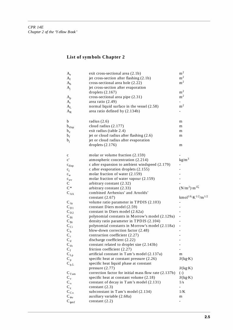
List of symbols Chapter 2
Ae exit cross-sectional area (2.1b) m2
Af jet cross-section after flashing (2.1b) m2
Ah cross-sectional area hole (2.22) m2
Aj jet cross-section after evaporationdroplets (2.167) m2
Ap cross-sectional area pipe (2.31) m2
Ar area ratio (2.49) -AL normal liquid surface in the vessel (2.58) m2
AR area ratio defined by (2.134b) -
b radius (2.6) mbdisp cloud radius (2.177) mbe exit radius (table 2.4) mbf jet or cloud radius after flashing (2.6) mbj jet or cloud radius after evaporation
droplets (2.176) m
c molar or volume fraction (2.159) -c' atmospheric concentration (2.214) kg/m3
cdisp c after expansion to ambient windspeed (2.179) -cj c after evaporation droplets (2.155) -cw molar fraction of water (2.159) -cwv molar fraction of water vapour (2.159) -C arbitrary constant (2.32) -C* arbitrary constant (2.33) (N/m2)⋅m3ζ
CAA combined Arrhenius’ and Arnolds’constant (2.67) kmol1/6⋅K1/2/m1/2
CAr volume ratio parameter in TPDIS (2.103) -CD1 constant Diers model (2.59) -CD2 constant in Diers model (2.62a) -CBi polynomial constants in Morrow’s model (2.129a) -CBr density ratio parameter in TPDIS (2.104) -CCi polynomial constants in Morrow’s model (2.118a) -Cb blow-down correction factor (2.48) -Cc contraction coefficient (2.27) -Cd discharge coefficient (2.22) -Cds constant related to droplet size (2.143b) -Cf friction coefficient (2.27) -CLp artificial constant in Tam’s model (2.137a) mCp specific heat at constant pressure (2.26) J/(kg⋅K)Cp,L specific heat liquid phase at constant
pressure (2.77) J/(kg⋅K)CTam correction factor for initial mass flow rate (2.137b) (-)Cv specific heat at constant volume (2.18) J/(kg⋅K)Cα constant of decay in Tam’s model (2.131) 1/sCε constant (2.3) -CCα subconstant in Tam’s model (2.134) 1/KCΦv auxiliary variable (2.68a) mCφmf constant (2.2) -
2.6
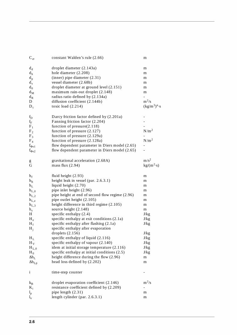
Cσ constant Walden’s rule (2.66) m
dd droplet diameter (2.143a) mdh hole diameter (2.208) mdp (inner) pipe diameter (2.31) mdv vessel diameter (2.68b) md0 droplet diameter at ground level (2.151) mdM maximum rain-out droplet (2.148) mdR radius ratio defined by (2.134a) -D diffusion coefficient (2.144b) m2/sDc toxic load (2.214) (kg/m3)n⋅s
fD Darcy friction factor defined by (2.201a) -fF Fanning friction factor (2.204) -F1 function of pressure(2.118) -F2 function of pressure (2.127) N/m2
F3 function of pressure (2.129a) -F4 function of pressure (2.128a) N/m2
fΦv1 flow dependent parameter in Diers model (2.65) -fΦv2 flow dependent parameter in Diers model (2.65) -
g gravitational acceleration (2.68A) m/s2
G mass flux (2.94) kg/(m2⋅s)
hf fluid height (2.93) mhh height leak in vessel (par. 2.6.3.1) mhL liquid height (2.70) mhL,0 pipe inlet height (2.96) mhL,2 pipe height at end of second flow regime (2.96) mhL,e pipe outlet height (2.105) mhL,3 height difference in third regime (2.105) mhs source height (2.148) mH specific enthalpy (2.4) J/kgHe specific enthalpy at exit conditions (2.1a) J/kgHf specific enthalpy after flashing (2.1a) J/kgHj specific enthalpy after evaporation
droplets (2.156) J/kgHL specific enthalpy of liquid (2.116) J/kgHV specific enthalpy of vapour (2.140) J/kgHL,0 idem at initial storage temperature (2.116) J/kgH0 specific enthalpy at initial conditions (2.5) J/kg∆hL height difference during the flow (2.96) m∆hLp head loss defined by (2.202) m
i time-step counter -
kB droplet evaporation coefficient (2.146) m2/sKi resistance coefficient defined by (2.209) -lp pipe length (2.31) mlv length cylinder (par. 2.6.3.1) m

CPR 14EChapter 2 of the ‘Yellow Book’
2.7
Lv heat of vaporisation (2.66) J/kgLv,w heat of vaporisation of water (2.161) J/kgLN(x) natural logarithm of argument x -10LOG(x) common logarithm of argument x -∆li distance along the pipe from rupture to
interface (2.126) m
n number of moles (2.9a) -Nt number of time-steps (2.12) -
p pressure ratio (2.47b) -pcr critical flow pressure ratio (2.47d) -pf final pressure ratio (2.47c) -P (absolute) pressure (2.8) N/m2
Pa ambient (atmospheric) pressure (2.1b) N/m2
Pc critical pressure of the chemical (2.11a) N/m2
Pe exit pressure in the pipe (2.1b) N/m2
Ph (hydraulic) liquid pressure (2.195) N/m2
Pi upstream pressure at interface (2.46) N/m2
PaL external pressure above liquid (2.195) N/m2
PR reduced pressure (2.11) -Pr Prandtl number (2.144c) -Pv˚ saturated vapour pressure (2.1d) N/m2
P0 initial pressure (2.95) N/m2
P* corrected pressure (2.118c) N/m2
∆P pressure drop (2.29a) N/m2
qS mass flow (discharge rate) (2.14) kg/sqS,e exit flow rate (2.121) kg/sqS,0 initial mass outflow (discharge) rate (2.35) kg/sqS,Φm=1 initial mass flow rate vapour only (2.82) kg/sQ (total) mass content (2.83) kgQH heat transferred into a system (2.18a) J/molQL liquid mass (2.71) kgQ0 initial total mass content (2.35) kgQV vapour mass (2.72) kgQV,0 initial vapour mass (2.81) kg
R gas constant (2.9a) J/(mol⋅K)Re Reynolds number (2.98) -RH relative humidity (2.157) -
sp circumference of a pipe (2.208) mSL specific entropy of liquid phase (2.111) J/(kg⋅K)SV specific entropy of vapour phase (2.111) J/(kg⋅K)
t time from the start of the outflow (2.12) st0 time when droplet reaches the ground (2.150) stv duration vapour blown-out (2.81) stB time constant in the Wilson model (2.35) stE maximum time validity model (2.42) s∆tE duration release remaining liquid (2.130b) s
2.8
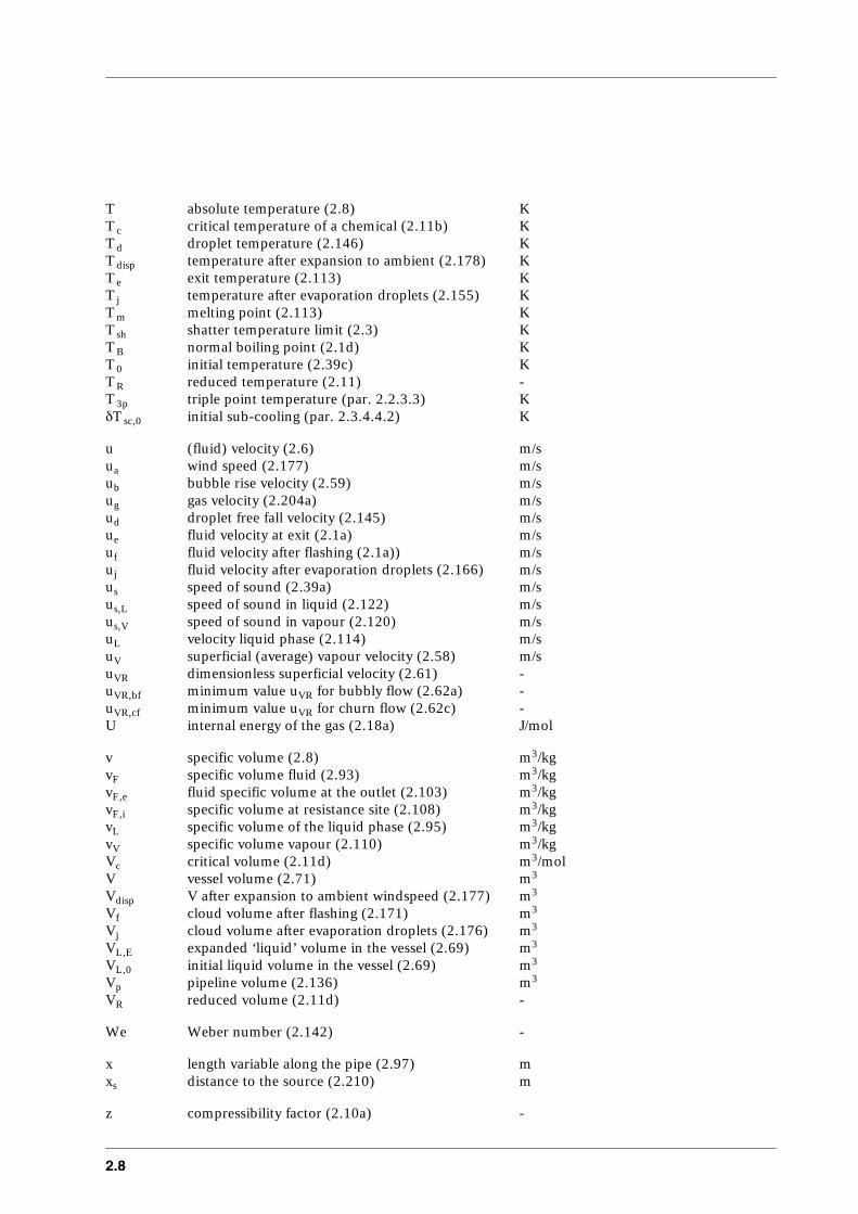
T absolute temperature (2.8) KTc critical temperature of a chemical (2.11b) KTd droplet temperature (2.146) KTdisp temperature after expansion to ambient (2.178) KTe exit temperature (2.113) KTj temperature after evaporation droplets (2.155) KTm melting point (2.113) KTsh shatter temperature limit (2.3) KTB normal boiling point (2.1d) KT0 initial temperature (2.39c) KTR reduced temperature (2.11) -T3p triple point temperature (par. 2.2.3.3) KδTsc,0 initial sub-cooling (par. 2.3.4.4.2) K
u (fluid) velocity (2.6) m/sua wind speed (2.177) m/sub bubble rise velocity (2.59) m/sug gas velocity (2.204a) m/sud droplet free fall velocity (2.145) m/sue fluid velocity at exit (2.1a) m/suf fluid velocity after flashing (2.1a)) m/suj fluid velocity after evaporation droplets (2.166) m/sus speed of sound (2.39a) m/sus,L speed of sound in liquid (2.122) m/sus,V speed of sound in vapour (2.120) m/suL velocity liquid phase (2.114) m/suV superficial (average) vapour velocity (2.58) m/suVR dimensionless superficial velocity (2.61) -uVR,bf minimum value uVR for bubbly flow (2.62a) -uVR,cf minimum value uVR for churn flow (2.62c) -U internal energy of the gas (2.18a) J/mol
v specific volume (2.8) m3/kgvF specific volume fluid (2.93) m3/kgvF,e fluid specific volume at the outlet (2.103) m3/kgvF,i specific volume at resistance site (2.108) m3/kgvL specific volume of the liquid phase (2.95) m3/kgvV specific volume vapour (2.110) m3/kgVc critical volume (2.11d) m3/molV vessel volume (2.71) m3
Vdisp V after expansion to ambient windspeed (2.177) m3
Vf cloud volume after flashing (2.171) m3
Vj cloud volume after evaporation droplets (2.176) m3
VL,E expanded ‘liquid’ volume in the vessel (2.69) m3
VL,0 initial liquid volume in the vessel (2.69) m3
Vp pipeline volume (2.136) m3
VR reduced volume (2.11d) -
We Weber number (2.142) -
x length variable along the pipe (2.97) mxs distance to the source (2.210) m
z compressibility factor (2.10a) -
CPR 14EChapter 2 of the ‘Yellow Book’
2.9
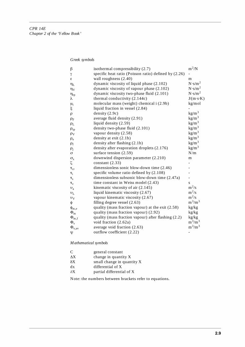
Greek symbols
β isothermal compressibility (2.7) m2/Nγ specific heat ratio (Poisson ratio) defined by (2.26) -ε wall roughness (2.40) mηL dynamic viscosity of liquid phase (2.102) N⋅s/m2
ηV dynamic viscosity of vapour phase (2.102) N⋅s/m2
ηtp dynamic viscosity two-phase fluid (2.101) N⋅s/m2
λ thermal conductivity (2.144c) J/(m⋅s⋅K)µi molecular mass (weight) chemical i (2.9b) kg/molξ liquid fraction in vessel (2.84) -ρ density (2.9c) kg/m3
ρF average fluid density (2.91) kg/m3
ρL liquid density (2.59) kg/m3
ρtp density two-phase fluid (2.101) kg/m3
ρV vapour density (2.58) kg/m3
ρe density at exit (2.1b) kg/m3
ρf density after flashing (2.1b) kg/m3
ρj density after evaporation droplets (2.176) kg/m3
σ surface tension (2.59) N/mσx downwind dispersion parameter (2.210) mζ constant (2.33) -τcr dimensionless sonic blow-down time (2.46) -τi specific volume ratio defined by (2.108) -τs dimensionless subsonic blow-down time (2.47a) -τv time constant in Weiss model (2.43) sυa kinematic viscosity of air (2.145) m2/sυL liquid kinematic viscosity (2.67) m2/sυV vapour kinematic viscosity (2.67) m2/sφ filling degree vessel (2.63) m3/m3
φm,e quality (mass fraction vapour) at the exit (2.58) kg/kgΦm quality (mass fraction vapour) (2.92) kg/kgΦm,f quality (mass fraction vapour) after flashing (2.2) kg/kgΦv void fraction (2.62a) m3/m3
Φv,av average void fraction (2.63) m3/m3
ψ outflow coefficient (2.22) -
Mathematical symbols
C general constant∆X change in quantity XδX small change in quantity Xdx differential of X∂X partial differential of X
Note: the numbers between brackets refer to equations.

2.10

CPR 14EChapter 2 of the ‘Yellow Book’
2.11
Glossary of terms
critical flow The critical (choked) outflow is reached whenthe downstream pressure is low enough for thestream velocity of the fluid to reach the sound ofspeed in the mixture, which is the maximumpossible flow velocity.
critical temperature The highest temperature at which it is possible tohave two fluid phases of a substance inequilibrium: vapour and liquid. Above thecritical temperature there is no unambiguousdistinction between liquid and vapour phase.
entropy Thermodynamic quantity which is the measureof the amount of energy in a system not availablefor doing work; the change of entropy of a systemis defined by ∆S = ∫ dq/T.
enthalpy Thermodynamic quantity that is the sum of theinternal energy of system and the product of itsvolume multiplied by its pressure: H = U + P⋅V.The increase in enthalpy equals the heatabsorbed at constant pressure when no work isdone other than pressure-volumetric work.
flashing or flash evaporation Part of a superheated liquid that evaporatesrapidly due to a relatively rapid depressurisation,until the resulting vapour/liquid-mixture hascooled below boiling point at the end pressure.
flow Transport of a fluid (gas or liquid or gas/liquid-mixture) in a system (pipes, vessels, otherequipment).
fluid Material of any kind that can flow, and whichextends from gases to highly viscous substances,such as gases and liquids and gas/liquid-mixtures; meaning not fixed or rigid, like solids.
head loss A measure for pressure drop related to thehydraulic liquid height.
physical effects models Models that provide (quantitative) informationabout physical effects, mostly in terms of heatfluxes (thermal radiation), blast due toexplosions, and environmental (atmospheric)concentrations.
piping Relatively short pipes in industrial plants.

2.12
pipelines Relatively long pipes for transportation of fluidchemicals.
pressurized liquified gas (pressure liquefied gas)Gas that has been compressed to a pressureequal to saturated vapour pressure at storagtemperature, so that the larger part hascondensed to the liquid state
quality The mass fraction of vapour in a liquid-vapourmixture (two-phase mixture).
release (synonyms: outflow, discharge, spill)The discharge of a chemical from itscontainment, i.e. the process and storageequipment in which it is kept.
saturation curve Saturation pressure as function of the (liquid)temperature.
saturation pressure The pressure of a vapour which is in equilibriumwith its liquid; also the maximum pressurepossible by vapour at given temperature.
source term Physical phenomena that take place at a releaseof a chemical from its containment beforeentering the environment of the failingcontainment, determining:– the amount of chemical entering the
surroundings in the vicinity of thecontainment, and/or release rate andduration of the release;
– the dimensions of the area or space in whichthis process takes place, including height ofthe source;
– the thermodynamic state of the releasedchemical, such as concentration, tempera-ture, and pressure;
– velocities of the chemical at the boundaries ofthe source region.
source term model Models that provide (quantitative) informationabout the source term, to be input into asubsequent physical effect model.
specific volume Volume of one kilogram of a substance;reciprocal of density ρ.
superheat The extra heat of a liquid that is available bydecreasing its temperature, for instance byvaporisation, until the vapour pressure equalsthat of its surroundings.
CPR 14EChapter 2 of the ‘Yellow Book’
2.13
triple point A point on a phase diagram representing a set ofconditions (pressure P3p and temperature T3p),under which the gaseous, liquid and solid phaseof a substance can exist in equilibrium. For apure stable chemical the temperature andpressure at triple point are physical constants.
two-phase flow Flow of material consisting of a mixture of liquidand gas, while the gas (vapour) phase isdeveloping due to the vaporisation of thesuperheated liquid during the flow, caused bydecreasing pressure along the hole or pipe due tothe pressure drop over the resistance.
vapour Chemical in the gaseous state which is inthermodynamic equilibrium with its own liquidunder the present saturation pressure at giventemperature.
void fraction The volume fraction of vapour in a liquid-vapourmixture (two-phase mixture).
Note: Some definitions have been taken from Jones [1992], AIChE [1989] andWebster [1981].

2.14
CPR 14EChapter 2 of the ‘Yellow Book’
2.15
Table of contents Chapter 2
Modifications to Chapter 2, Outflow and Spray release ......................3
List of symbols Chapter 2 ......................................................................5
Glossary of terms .................................................................................11
2 Outflow and Spray release...................................................................172.1 Introduction..................................................................................172.2 Phenomenon of outflow ................................................................19
2.2.1 Introduction to section 2.2...................................................192.2.2 Pressure and resistance ........................................................192.2.3 Thermodynamic state of the stored chemical ........................202.2.4 Release modes.....................................................................26
2.3 General overview of existing models...............................................292.3.1 Introduction to section 2.3...................................................292.3.2 Release modes.....................................................................292.3.3 Compressed gases................................................................312.3.4 Pressurised liquefied gases ...................................................322.3.5 Liquids ...............................................................................512.3.6 Friction factors ....................................................................532.3.7 Physical properties of chemicals ...........................................53
2.4 Selection of models .......................................................................552.4.1 Introduction to section 2.4...................................................552.4.2 Gases ..................................................................................552.4.3 Pressurised liquefied gases ...................................................562.4.4 Liquids ...............................................................................60
2.5 Description of models ...................................................................612.5.1 Introduction to section 2.5...................................................612.5.2 Compressed gases................................................................632.5.3 Pressurised liquefied gases ...................................................782.5.4 Liquids .............................................................................1182.5.5 Friction factors ..................................................................123
2.6 Application of the selected models: calculation examples ..............1272.6.1 Introduction to section 2.6.................................................1272.6.2 Compressed gases..............................................................1272.6.3 Pressurised liquefied gases .................................................1342.6.4 Liquids .............................................................................153
2.7 Interfacing to other models ..........................................................1572.7.1 Introduction to section 2.7.................................................1572.7.2 Interfacing to vapour cloud dispersion models ....................157
2.8 Discussion of outflow and spray release models ............................1672.8.1 Introduction to section 2.8.................................................1672.8.2 General remarks ................................................................1672.8.3 Single-phase (out)flow and vessel dynamics ........................1682.8.4 Pressurized liquified gases ..................................................1682.8.5 Spray release mode to reacting chemicals............................1692.8.6 ‘Epilogue’..........................................................................169
2.9 References ..................................................................................171

2.16
Appendix 2.1 Some properties of chemicals used in the TPDIS model [Kukkonen, 1990]
Appendix 2.2 Relations for changes in enthalpy and entropy
CPR 14EChapter 2 of the ‘Yellow Book’
2.17
2 Outflow and Spray release
2.1 Introduction
Many hazardous materials are stored and transported in large quantities ingaseous and, usually, in liquid form, refrigerated or under pressure.Incidental releases of hazardous materials can arise from failures in the process orstorage equipment in which the hazardous substance is kept in a safe condition. Initiating events are either system internal or system external. Internal causes may besubdivided into those arising from departures from design condition during operationand those from human error in operation. External causes could be, for instance,failure through mechanical impact, natural causes, corrosion and domino effectswhich are events arising at one plant affecting another. Releases may also be necessary for the operation of a process.The release of a material depends on:– the physical properties of the hazardous material;– the process or storage conditions;– the way the (accidental) decontainment takes place, and,– possible subsequent mechanical and physical interaction with the environment.
The state of aggregation of a chemical is determined by its physical properties, andthe process or storage conditions, i.e. pressure and temperature in the containment.For mixtures of chemicals also the composition has to be known.The Yellow Book deals with gases and liquids, so the following process conditions areconsidered, as usual:1. compressed gas,2. pressurised liquefied gases,3. liquids.
Incidental releases from containment systems range from slow discharge through asmall pinhole failure to rapid discharge resulting from a major rupture of acontainment; Jones [1992].
During and after a release, the released material, gas or liquid, may interact with theimmediate surroundings in its own specific way, also depending on the processconditions. These interactions have a direct effect on the (thermodynamic) state ofthe hazardous material entraining into the surroundings. The released material mayform a liquid pool, or may be dispersed into the atmosphere or into a water body, ormay be ignited immediately.
The models in this chapter ‘Outflow and Spray Release’ may act as a source termmodel to provide (quantitative) information about the so-called source term, such as:– the amount of material entering the surroundings in the vicinity of the failing
containment;– the dimensions of the area or space in which this process takes place;– the thermodynamic state of the released chemicals: concentration, temperature,
and pressure;– velocities of the outflowing chemical at the boundaries of the source region.
2.18
These results may be used for further calculations as input for subsequent physicaleffect models, described in chapter 3 ‘Pool evaporation’, in chapter 4 ‘Vapour CloudDispersion’, and in chapter 6 ‘Heat flux from fires’.
In the following sections, release phenomena of gases/vapours and liquids undervarious conditions will be addressed. Each section will treat the subject from anotherperspective.Section 2.2 provides the principles and basic understanding of the phenomena ofoutflow and spray release. It will address the applied thermodynamics and transportlaws.Section 2.3 provides an overview of methods and models published in open literatureregarding the estimation of the characteristics of releases: release rates, temperaturesof the released chemical, etc.In section 2.4 the considerations will be elucidated that have led to the selection ofthe recommended models.Section 2.5 provides complete detailed descriptions of the recommended models andmethods. Whenever calculations or analyses have to be made, all necessaryinformation can be found in this chapter, except for the physical properties of thechemical.Section 2.6 provides examples in using the selected models and methods.In section 2.7 the interfacing of other models, i.e. the necessary transformation of theresults, will be addressed.Finally, in section 2.8 general considerations are given about the models and methodspresented and present gaps in the knowledge about outflow and spray release.

CPR 14EChapter 2 of the ‘Yellow Book’
2.19
2.2 Phenomenon of outflow
2.2.1 Introduction to section 2.2
Section 2.2 provides the principles and basic understanding of thephenomenon of outflow (and spray release).The outflow through an opening in a containment is mainly controlled by:1. The pressure in the containment and the resistance to flow through the opening,
and,2. The state of aggregation of the chemical: gas, liquid, or vapour/liquid-mixture.
The different modes of a release can be divided in:1. Transient releases (outflow), and,2. Instantaneous releases.
The effect of pressure and resistance is briefly addressed in subsection 2.2.2.The influence of the aggregation state of the outflowing fluid chemical is explained insubsection 2.2.3.In subsection 2.2.4 mainly the distinction between stationary and non-stationaryoutflow is addressed in detail, determining the concept of modelling.
2.2.2 Pressure and resistance
The driving force for outflow of a material from a containment is thepressure difference between the containment and the ambient. Such overpressure may exist because of:1. gas compression,2. saturated vapour pressure at storage temperature, or, 3. hydraulic liquid height.
The pressure difference has to overcome the wall friction due to flow in pipes and pipefittings. Friction causes a pressure drop depending on the roughness of the pipe walland the shape of the pipe fittings. Friction factors relate the pressure drop caused byfriction to the characteristics of the pipe, such as pipe diameter and roughness of theinner pipe wall, and the flow velocity and the viscosity of the fluid.
In general the outflow rate of fluids will increase if the pressure difference over thehole or pipe increases, and thus also the stream velocity. Flow of compressible fluids,like gases and vapour/liquid-mixtures (two-phase mixtures) may become critical. The so-called critical (choked) outflow is reached when the downstream pressure islow enough for that the stream velocity of the fluid to reach the speed of sound in themixture, which is the maximum flow velocity possible. For a given constant upstreamstagnation state, further lowering of the downstream pressure does not increase themass flux, but will only lead to steep pressure drops in the opening to the ambient. When the upstream pressure increases, the critical mass flow rate (kg/s) will increasebut only due to the increasing density of the outflowing chemical.

2.20
If the pressure in the outlet is higher than the ambient pressure, the flow is calledchoked. If these pressures are (nearly) equal, the flow is non-choked. It is customaryto use ‘choked flow’ and ‘critical flow’ as synonyms.
2.2.3 Thermodynamic state of the stored chemical
The state of aggregation of a chemical is determined by its physicalproperties and the process or storage conditions, i.e. pressure and temperature in thecontainment. For mixtures of chemicals also the composition has to be known.
This book deals with gases and liquids, and so the following different processconditions are considered, as usual:1. compressed gas,2. pressurised liquefied gases,3. liquids.
2.2.3.1 Gases
‘State of aggregation of chemical or mixture of chemicals that is fully in thegaseous state under the present pressure and temperature; gases have neither independentshape nor volume [Webster, 1981].’
If the temperature T of a chemical is higher than its critical temperature Tc, it will bea gas. Below the critical temperature the chemical may still be a gas if the pressure Pis lower than the saturated vapour pressure Pv˚(T). Increasing the pressure above itssaturated vapour pressure at given temperature, forces the chemical to condensate.
2.2.3.2 Liquids
‘State of aggregation of a chemical or mixture of chemicals, in which it has adefinite volume but no definite form except that given by its container [Webster, 1981].’
If a chemical has a temperature between its boiling point TB(P) at given (partial)pressure P and its melting point Tm, it will be in the liquid state. Often these liquidsare called non-boiling liquids, to distinguish them from the liquid phase apparent instored pressurised liquefied gases.It must be mentioned, however, that the mere fact of boiling or not boiling of theliquid is not relevant for outflow. Just the fact that the vapour pressure of a (non-boiling) liquid may be neglected if it is less than atmospheric, is relevant.Refrigerated liquefied gases (just) below atmospheric pressure are also non-boilingliquids.
CPR 14EChapter 2 of the ‘Yellow Book’
2.21
2.2.3.3 Pressurised liquefied gases
‘Chemical in the liquid state which is in thermodynamic equilibrium with its ownvapour under the present saturation pressure at given temperature, higher than theatmospheric pressure.’
The usual term ‘pressurised liquefied gases’ refers to a state in which a liquidchemical, i.e. the condensed ‘gas’, is in thermodynamic equilibrium with its ownvapour, and thus at saturation pressure at given temperature: P=Pv˚(T).The use of the terminology about ‘gases’ and ‘vapours’ used in this respect may be alittle awkward, but will be maintained while commonly used in practice.
A so-called ‘pressurised liquefied gas’ is basically a two-phase system in which thevapour phase is in thermodynamic equilibrium with the liquid phase. This liquid-vapour equilibrium may exist along the saturation curve: the storage temperaturemust be between the critical temperature Tc and the triple point temperature T3p ofthe chemical.
2.2.3.4 Influence of thermodynamic state of the stored chemical
The different thermodynamic states a chemical can have, have a majorinfluence on the outflow in two ways. First, the magnitude of the mass outflow rateis very dependent on the aggregation state of the fluid. Secondly, the thermodynamicstate of the chemical in the vessel determines to a great extent the way in which thevessel will react to the loss of material resulting from the outflow.
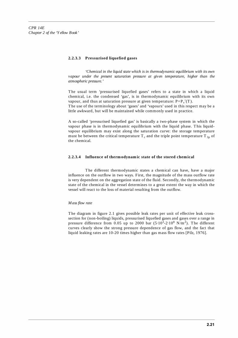
Mass flow rate
The diagram in figure 2.1 gives possible leak rates per unit of effective leak cross-section for (non-boiling) liquids, pressurised liquefied gases and gases over a range inpressure difference from 0.05 up to 2000 bar (5⋅103-2⋅108 N/m2). The differentcurves clearly show the strong pressure dependence of gas flow, and the fact thatliquid leaking rates are 10-20 times higher than gas mass flow rates [Pilz, 1976].
2.22
Figure 2.1 Mass flow rate versus pressure difference for flow of gases, vapours and liquids through an orifice [Pilz, 1976]
Two-phase flow
Beside gas flow and liquid flow, a so-called two-phase flow may be apparent. In general a ‘two-phase flow’ is basically a fluid flow consisting of a mixture of twoseparate phases, for instance water and oil, or water and air.In this chapter we consider only two-phase flows of a pure, single chemical. Such two-phase flows may develop when a pressurised liquefied gas flows through apipe and the local pressure in the pipe becomes lower than the saturation pressure ofthe flowing liquid, due to decrease of pressure along the pipe due to friction. Then the liquid becomes superheated and a gas phase may appear due to vaporisationof the liquid.
The most important factor in the two-phase flow is the volumetric void fraction ofvapour in the liquid (or its mass equivalent: quality). The quality determines to a largeextent the mass flow rate and the friction in the pipe.The largest possible discharge rate is obtained with a pure liquid phase flow. For atwo-phase discharge the mass flow rate may be substantially smaller, due to theincreased specific volume of the fluid.
Two-phase flow occurs if a pressurised liquefied gas is flowing in a pipe. This is acomplex physical process, and a concise description of the process will be given here.Liquid, from the liquid section of the vessel filled with pressurised liquefied gas,accelerates into the pipe entrance and experiences a pressure drop. Regarding initiallysaturated liquids which are per definition in thermodynamic equilibrium with theirvapour phase, this pressure drop creates a superheated state and nucleation bubblesare formed, when the pressure decreases below the saturation pressure.
CPR 14EChapter 2 of the ‘Yellow Book’
2.23
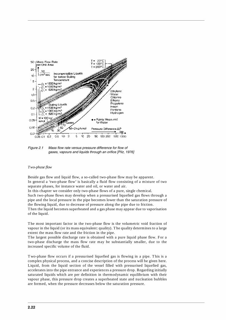
The (rapidly) vaporising liquid (flashing) is part of a bubble formation process inwhich subsequently the formation of vaporisation nuclei, bubble growth and bubbletransport take place. The flashing process is related to the vaporisation of liquidaround nuclei and the hydrodynamics of the liquid under thermodynamic non-equilibrium conditions. Vaporisation nuclei develop under the influence of micro-cavitation at the pipe surface on the inside, as shown in figure 2.2.
Figure 2.2 Flash vaporisation of a pressurised liquefied gas in a pipe [Yan, 1990]
The driving force for liquid evaporation is therefore its excessive temperature abovethe saturation curve corresponding to the local pressure. Evaporation is usuallyconsidered to occur at the liquid bubble interface, and bubbles may continue to formdownstream. Further continuous pressure losses arise due to liquid wall friction and,more importantly, due to the evaporation process. As a result, the degree of superheattends to increase and consequently also the evaporation rate. In addition, theexpanding bubbles begin to interact and coalesce and adopt different heat and masstransfer modes: bubble flow, churn turbulent flow.In many flows the evaporation proceeds to a point where the liquid is forced to thepipe walls and the gas occupies a rapidly moving core: annular flow.
2.24
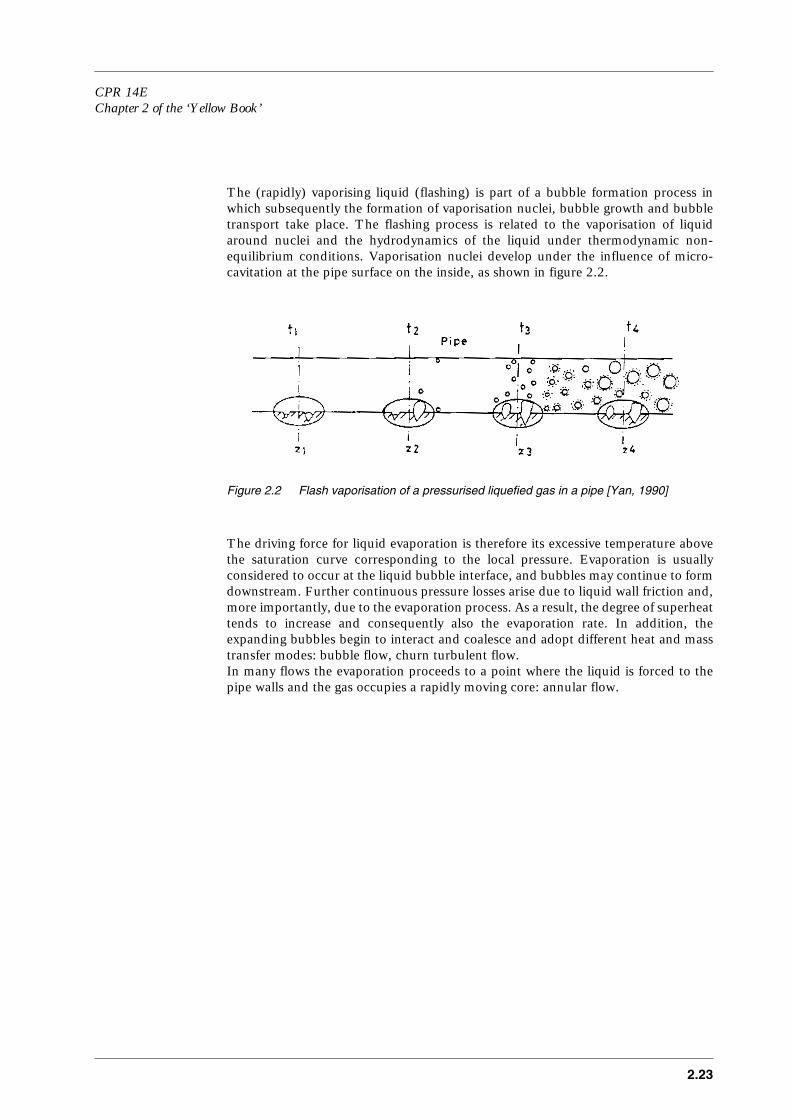
Figure 2.3 Schematic of superheated liquid pipe flow [Ewan, 1988]
In critical flows, the acceleration has progressed to the point where the flow is choked,which is characterised by very steep pressure gradients located at the pipe exit, wherethe pressure is above ambient.
The maximum fraction of pressurised liquefied gas that may flash (vaporise) occurswhen the final pressure is equal to the atmospheric pressure. During flashing, the totalentropy of the fluid is conserved. Often it is assumed that the fluid is in a saturatedstate initially and finally, and the fluid is initially pure liquid (quality Φm,0 = 0). Thefinal temperature of the fluid leaving the pipe, is the boiling point temperature.In choked isentropic pipe flow the vapour fraction of the fluid at the exit is alwayssmaller than the maximum flash fraction, because the exit pressure is higher than theatmospheric pressure for choked (critical) pipe flow. Small qualities correspond to apartial flashing process in which the exit pressure is substantial.

CPR 14EChapter 2 of the ‘Yellow Book’
2.25
Note that although the discharged fluid is mostly liquid on the basis of mass, it ismostly vapour on the basis of volume. The qualities of a few per cent correspond tovapour volume fractions larger than 90%. Clearly, this is due to the fact that thedensity of liquid is two to three hundred times higher than the density of vapour[Kukkonen, 1990].
Behaviour vessel content (‘vessel dynamics’)
For gases the position of the opening in the containment is irrelevant in general,although depressurising gas mixtures may partially condensate on the wall of thecontainment, resulting in a liquid pool at the bottom.
In case of a pressurised liquefied gas, a rapid depressurisation causes the liquid in thevessel to flash, which means that due to a relatively rapid depressurisation part of asuperheated liquid evaporates rapidly until the resulting vapour/mixture is cooledbelow boiling point at the end pressure. Due to the development of vapour bubblesin the stored liquid (‘champagne-effect’) the liquid phase seems to expand,necessitating a redefinition of liquid height. If the expanded liquid rises above the hole in the tank, a two-phase flow will beapparent through the hole in the tank. The level swell is illustrated in figure 2.4.
Figure 2.4 Illustration of level swell in a depressurizing vessel filled with pressurised liquefied gas [Wilday, 1992]
It might not be realistic to expect a homogeneous rise of the liquid level in the vessel.During the blow down of the vapour, initially apparent in the vapour section of thevessel, liquid might be dragged along through the opening.However, little data exist for the transient void fraction in the vent line during rapiddepressurisation. Experiments have been carried out in which the blow-down timeswere less than two seconds [Bell, 1993]. It was concluded that the quality inside thevent line, based on the calculated vessel-average values, was much less than theexperimentally determined values. This effect may compensate neglected apparent
2.26
liquid dragged along with the vapour stream.Altogether it may be concluded, that the some-what idealised approach of having ablow-off of the vapour initially apparent, until the swelled liquid has risen above theopening in the vessel, may be not too bad an approximation.So, for pressurised liquefied gases the relative height of the liquid level above theoutflow opening in the containment is a crucial factor in determining the initialquality of the outflowing material from the vessel:1. (Small) hole in vapour space of the vessel
well above liquid level: → vapour outflow2. Hole in vapour space just above liquid level: → two-phase flow3. Hole in liquid space well below liquid level: → liquid outflow
In case of pressurised liquefied gases and non-boiling liquids the shape of the vesselshould be taken into account for estimation of the liquid height. This height might beof importance for the relative height of the hole or pipe connection and the hydraulicpressure.Liquids will flow out as long as the liquid level is higher than the opening.
2.2.4 Release modes
Incidental releases from containment systems range from slow dischargethrough a small pinhole failure to rapid discharge resulting from a major rupture of acontainment [Jones,1992].
In case a vessel has been damaged to a minor extent, this results in a small openingto the environment leading to relatively small outflow rates compared to the totalamount of hazardous material in the process. This opening could be a crack or holein the vessel wall, or could be a rupture of connected piping with a relatively smalldiameter. Depending on the ratio between the (initial) transient outflow rate and thetotal mass of chemical stored, a transient outflow has to be regarded as non-stationaryor as (quasi-)stationary.
In general for outflow from vessels through a hole and through piping, the flow canbe considered to be stationary, meaning that the outflow is (fully) controlled by the(stagnant) upstream pressure and the downstream pressure.If the conditions upstream are changing gradually in time, the flow may be consideredquasi-stationary, meaning that the outflow rate is changing in time only because theconditions upstream are changing.
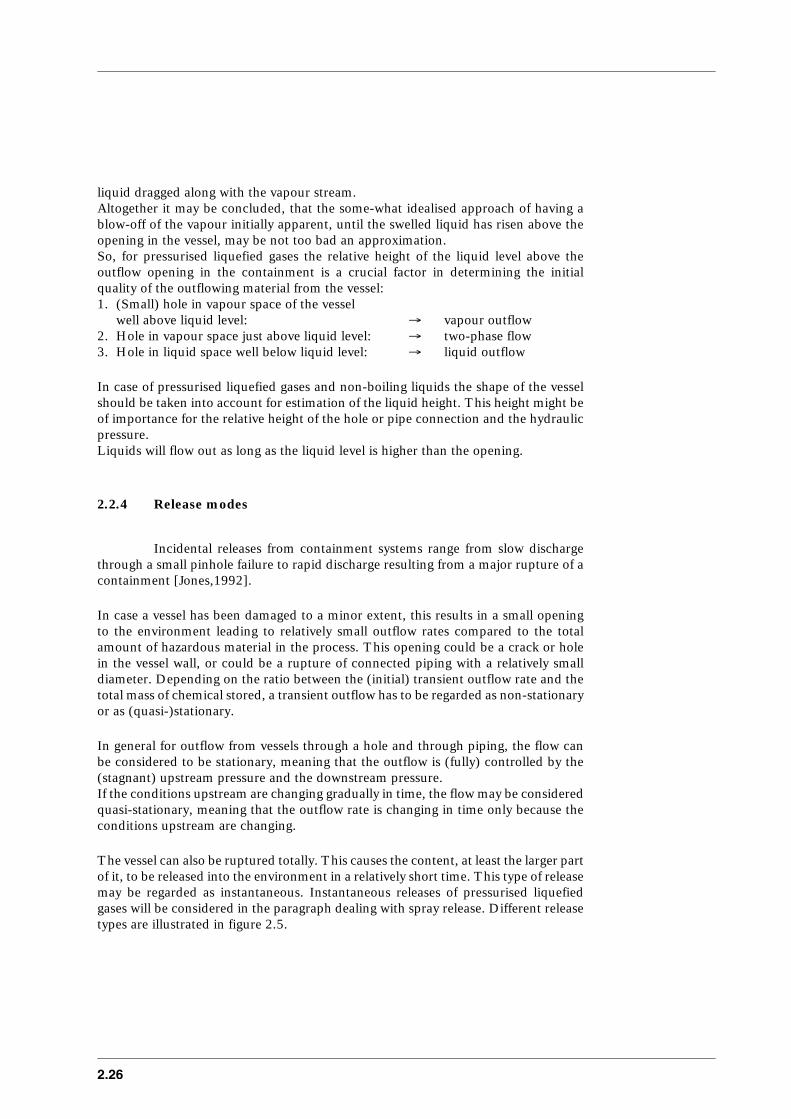
The vessel can also be ruptured totally. This causes the content, at least the larger partof it, to be released into the environment in a relatively short time. This type of releasemay be regarded as instantaneous. Instantaneous releases of pressurised liquefiedgases will be considered in the paragraph dealing with spray release. Different releasetypes are illustrated in figure 2.5.
CPR 14EChapter 2 of the ‘Yellow Book’
2.27
Figure 2.5 llustration of some conceivable release mechanisms [Kaiser, 1988]
In case of ruptured pipelines the flow in the pipeline will not be stationary during thelarger part of the outflow, meaning that the outflow is not being controlled by the(stagnant) conditions of both pipe ends only, but will also be a function of time afterthe rupture itself.

2.28
CPR 14EChapter 2 of the ‘Yellow Book’
2.29
2.3 General overview of existing models
2.3.1 Introduction to section 2.3
Section 2.3 provides an overview of methods and models for estimation ofthe characteristics of releases: release rate and thermodynamic state of the releasedchemical.
In the previous section the following different process conditions have beenconsidered:1. compressed gas,2. pressurised liquefied gases,3. (non-boiling) liquids.The main structure of this section will be along this classification.
In the previous section also the following release modes have been distinguished:1. outflow from vessels,2. outflow from pipelines,3. total rupture of vessels.For each process condition these three different release modes have to be addressed.
While the way of modelling of the different release modes is typical for every processcondition, the general features of the approaches concerning the different releasemodes will be explained in subsection 2.3.2 first.In subsection 2.3.3 the outflow of compressed gases will be explained, in subsection2.3.4 the outflow of pressurised liquefied gases and in subsection 2.3.5 the outflow of(non-boiling) liquids. In general physical properties are required to perform the calculations. For thecalculations of the mass flow rate for flow in pipes, friction factors are required.Finally, in subsections 2.3.6 and 2.3.7 these two topics will be briefly addressed.
2.3.2 Release modes
2.3.2.1 Quasi-stationary flow from vessels
For outflow through relatively small holes in a vessel wall or in piping theflow may be considered to be quasi-stationary, as the vessel conditions changerelatively gradually. Transient conditions in the hole or pipe may be neglected.The flow of a chemical out of a containment with a large capacity relative to theoutflow rate, can be described by two coupled independent sub-models:1. a sub-model ‘vessel dynamics’ that describes the dynamic behaviour of the
material stored in the containment,2. a sub-model ‘outflow’ that predicts the outflow rate and the conditions of the
outflowing material as function of the conditions in the containment.

2.30
The independency of the ‘outflow’ and the ‘vessel dynamics’, makes it possible toestimate the change of the vessel conditions, regardless whether:1. the outflow of materials goes through piping or through a hole in the vessel wall,2. the gas outflow is critical or sub-critical (choked or non-choked),3. the loss of containment is due to a one-phase outflow through a hole in the vessel
wall or a two-phase flow in a pipe, etc.
The sub-model ‘vessel dynamics’ covers the changes of pressure, temperature, andmass content in the vessel caused by the outflow of material.The changes of the conditions in the vessel may be estimated for small steps, i.e.sufficiently short periods of time, assuming the outflow rate and physical propertiesof the stored material to be constant. This approach accommodates handling of discontinuities in the behaviour of thevessel content, like the ‘sudden’ drop of the liquid level under the vessel hole or pipeconnection. In case the outflow rate effects the dynamic behaviour in the tank thenfor every time-step an iterative solution is still required.The dependency of physical properties of temperature and pressure in the vessel caneasily be taken into account, avoiding analytical approximations.Usual assumptions made are thermodynamic equilibrium, isentropic processes, andhomogeneous liquid and vapour or gas phases in the vessel.A process is called isentropic when it is adiabatic and thermodynamic reversible. Theassumption of adiabatic process may be a good approximation for relatively badlyisolated systems when the quantity of mass flowing through is so big that any heatexchange can be neglected.
2.3.2.2 Non-stationary flow from pipelines
In case of a rupture of a pipeline the flow in the pipe itself is non-stationary.The flow is controlled by the initial conditions in the pipeline apparent before therupture, the ambient conditions, and the time passing after the rupture.The models may be distinguished according to the different process conditions1. gas pipelines,2. liquid pipelines,3. pipelines with pressurised liquefied gases.For non-stationary flows the usual assumptions regarding thermodynamicequilibrium can not be made without careful examination.
2.3.2.3 Total rupture of vessels: instantaneous releases
The physical phenomena playing a roll with instantaneous release of gasesand (non-boiling) liquids are incorporated in ‘subsequent’ models, respectivelyvapour cloud dispersion (chapter 4) and pool evaporation (chapter 3), and will not beaddressed in this chapter. The instantaneous release of pressurised liquefied gases is not trivial and independentmodelling exist. This topic will be addressed in the subsection 2.3.4.7

CPR 14EChapter 2 of the ‘Yellow Book’
2.31
2.3.3 Compressed gases
2.3.3.1 Introduction to compressed gases
The (out-)flow of gases through holes and in pipes, and the dynamicbehaviour of a (adiabatic) expansion of a compressed gas in a vessel, have been wellestablished for many years. The governing equations can be found in any handbookon this matter.
2.3.3.2 Vessel dynamics compressed gas
Due to the outflow of gas out of a containment (vessels or pipelines), theremaining gas rapidly depressurises and will expand. This inevitably leads to areduction in the temperature of the gas and the vessel itself. In case of gas mixturesless volatile components may condensate [Haque, 1990].
Applying the first law of thermodynamics, using the definition of volumetric workdone by an expanding gas and of equations of state for (non-)perfect gases, enablesthe prediction of the decrease of pressure and temperature during the outflow.This will result in an adequate description of the vessel dynamics as will be describedin section 2.5.
2.3.3.3 Gas flow through holes and piping
Well-known relations for the stationary outflow through orifices andthrough pipes exist. In the previous edition [YellowBook,1988] models for criticaland non-critical gas flow through holes have been given, together with laminar andturbulent flow of fluids (i.e. gases and liquids). These models will be described insection 2.5.
Vapour flow
The models for outflow of gas through holes and through piping are also valid for purevapour flowing out of the vapour section in the containment for vaporisingpressurised liquefied gases.
2.3.3.4 Non-stationary gas flow in pipelines
Non-stationary gas flow after a full bore pipeline rupture
The previous edition of the YellowBook [1988] describes an approximate solution ofthe set differential equations governing the non-stationary gas flow after a full borepipeline rupture by linearisations and applying perfect gas law. The time-dependency

2.32
of the outflow is treated by assuming a so-called expansion zone which, after full borerupture, starts moving with the speed of sound in the pipeline in the opposite(upstream) direction. This model has not been validated.
Both Olorunmaiye [1993] and Lang [1991] describe two rather complex models withcorresponding numerical solution procedures. Assumptions made are: one-dimensional flow, friction term as in steady flow, isothermal or adiabatic flow, perfectgas.Lang [1991] describes the flow in the gas pipeline after breakage by solving the massbalance and momentum differential equation using the spectral method withLegrendre-polynomials. Olorunmaiye [1993] recognises the conservation equations for mass and momentumto form a set of hyperbolic partial differential equations, and solves them with anumerical method of characteristics.
Hanna [1987] gives the empirical correlation of Bell, as reformulated by Wilson. TheWilson model predictions for the mass flow rate of methane from a pipeline are quitesimilar to those of the Gasunie-model.
Non-stationary gas flow in pipelines through small holes
In Weiss [1988] an empirical correlation has been given for small leakages inpipelines, which has been validated against complex models. This correlation for small holes in pipelines is the only model found in open literature.
2.3.4 Pressurised liquefied gases
2.3.4.1 Introduction to pressurised liquefied gases
After a (sudden) depressurisation the liquid in the vessel will flash, and dueto the presence of vapour bubbles in the tank the liquid section will expand(‘champagne effect’), necessitating a redefinition of liquid height. When the expanded liquid rises above the hole in the tank a two-phase flow will beapparent through the opening in the tank, in stead of a pure vapour outflow.Qualitatively the following situations for outflow of pressurised liquefied gases from avessel may occur:1. (small) hole in vapour space of the vessel well
above liquid level: vapour outflow2. hole in vapour space near initial liquid level: two-phase flow3. hole in liquid space (well) below liquid level: liquid outflow
So, for pressurised liquefied gases the height of the liquid level relative to the outflowopening in the containment, is an important factor determining the initial state of theoutflowing material from the vessel, and thus the behaviour of the vessel content(‘vessel dynamics’). In order to determine which flow type will initially be at hand,the rise of the boiling liquid due to the bubble formation relative to the position of theopening in the vessel should be estimated first.

CPR 14EChapter 2 of the ‘Yellow Book’
2.33
Furthermore, the outflow from the vessel may be through a hole or short pipe, orthrough a pipe.In the scheme below a survey is given of the possible situations concerning the outflowof pressurised liquefied gas from a containment. The description of the varioussituations will be according to this diagram.
Diagram 2.1 Different situations concerning the outflow of pressurised liquefied gas from containment
In the following section the vessel dynamics of stored pressurised liquefied gases forthe different outflow types will be addressed first in paragraph 2.3.4.2.The outflow through holes and piping for each of the different flow types, will beaddressed in paragraphs 2.3.4.3 and 2.3.4.4 respectively.In paragraph 2.3.4.5 the two-phase flow in pipelines will be addressed.
2.3.4.2 Vessel dynamics pressurised liquefied gases
2.3.4.2.1 Flow type inside the vessel
Fauske [1988] gives simple criteria that may determine whether there existsa two-phase flow inside the vessel or not. Fauske has presented simple vapourdisengagement rules for determining the release type of non-foamy materials.Especially if the liquid is viscous (e.g. greater than 500 cP) or has a tendency to foam,two-phase flow in the containment will be apparent [AIChE, 1989].
Melhem [1993] describes a refined DIERS-method that distinguishes different waysof boiling in case of top venting, and relations to estimate the quality in the outflowopening for vertical vessels. From Sheppard [1993] it appears that the analytical
I) Quasi-stationary outflow from vessel:
1) Vapour outflow (2.3.4.2.3):a) Through hole in vessel wallb) Through piping
2) Two-phase outflow (2.3.4.2.4):a) Through hole in vessel wallb) Through piping
3) Liquid outflow (2.3.4.2.5):a) Through hole in vessel wallb) Through piping
II) Non-stationary outflow from pipeline (2.3.4.5):
a) Due to full bore ruptureb) Through hole in pipe wall

2.34
solution of the DIERS-model validates the Fauske correlation. This analyticalsolution has been shown to hold for varying cross-sectional vessels.
The DIERS-model SAFIRE [Skouloudis, 1990] is a complex model requiringextensive thermophysical data [AIChE, 1989]. However, in Sheppard [1994] it hasbeen concluded that the numerical DIERS-model underpredicts the void fraction forvertical vessels for bubbly flow.
2.3.4.2.2 Void fraction in the vessel
The expansion of a rapid boiling liquid depends on the ratio of the outflowrate and the size of the vaporisation area of the boiling liquid.Belore [1986] gives the correlation of Mayinger to estimate the void fraction in theexpanded liquid. The void fraction or hold-up in a flashing liquid due todepressurisation is calculated using Viecenz experimental correlation, as published byMayinger in 1981 [Belore, 1986].
For large atmospheric containers the liquid swell may be principally due to the boilingtwo-phase boundary layer, in the absence of vapour carry-under, so the major part ofthe bulk liquid remains bubble free. The two-phase flow effects for non-foamysubstances can be ignored as long as liquid entrainment at the interface is preventedensuring low vapour velocities. However, the present state of knowledge about theeffects of bulk liquid sub-cooling on mitigating the liquid swell permits only case bycase numerical solutions involving sizeable computer programs [Sallet, 1990,3].
The depressurisation of a pressurised liquefied gas causing bubble formation in theliquid and thus expansion of the boiling liquid is a rather complex phenomenon.A large computer model has been presented by Haque [1992]. Although it deals withgas-oil-water mixtures, it demonstrates the complexity of the process by showing thevarious factors that influence the behaviour of the boiling liquid in the vessel.For instance, the heat flux between the different phases and between the vessel andthe surroundings, are taken into account. During a ‘blow-down’ large temperaturegradients in the vessel may be apparent.
2.3.4.2.3 Vessel dynamics vapour outflow (quality=1)
Vessel dynamics are mainly controlled by the evaporation of the pressurisedliquefied gas, which is assumed to be at saturated vapour pressure initially.Due to the outflow of vapour the vessel depressurises. This causes the liquefied gasto evaporate, and subsequently the temperature will decrease and so will the saturatedvapour pressure. More details can be found in section 2.5.
2.3.4.2.4 Vessel dynamics two-phase outflow (0<quality<1)
The model for two-phase outflow from a vessel is similar to the one foroutflow of only vapour. Additional assumptions are that the two-phase mixture in the

CPR 14EChapter 2 of the ‘Yellow Book’
2.35
vessel is considered to be homogeneous, and that the quality of the outflowingmaterial is identical to that of the vessel. More details can be found in section 2.5.
The quality in the vessel, and so the ratio between the vapour and liquid mass,changes due to the evaporation of liquid in the vessel caused by the depressurisation.Sumathipala [1990] states that the average void fraction is not representative of thelocal void fraction in the vessel. The void fraction in the top of the vessel venting maybe much higher than the average value. This is demonstrated in the figure 2.6.Also Bell [1993] concludes that the void fraction in the vent line is much higher thanin the vessel. This corresponds to a lower mass flow rate and also to a highervolumetric flow rate. This criticism can only be coped with by applying verycomplicated models.
Figure 2.6 Top venting with flashing fluid [Bell, 1993]
2.3.4.2.5 Vessel dynamics of liquid outflow (quality=0)
In this case vessel dynamics are mainly controlled by saturated vapourpressure of the liquid at vessel temperature.Due to the outflow of liquid the vessel depressurises. While the density of the vapouris much lower than the liquid, a relatively small amount of liquid has to evaporate inorder to maintain the pressure, and the temperature drop will be relatively small.The model for liquid outflow from a vessel filled with pressurised liquefied gas is quitesimilar to the one for outflow of only vapour. Here it is assumed that the change ofvapour mass in the vessel is caused by evaporation of liquid only.The estimation of the vessel conditions is similar to the model for the vapour outflow.In addition, the new liquid height has to be estimated as a function of the remainingliquid mass.More details can be found in section 2.5.

2.36
2.3.4.3 Outflow of pressurised liquefied gas through a hole in vessels
Vapour outflow
The models for outflow of gas through holes are valid for pure vapour flowing out ofthe vapour section in the containment from vaporising pressurised liquefied gases.
Two-phase outflow through a hole: champagne outflow
In the previous edition of the [YellowBook, 1988] the outflow of a two-phase mixturethrough a hole has been described assuming a fluid having a density based on thevapour mass fraction or quality. This approach is commonly applied, WorldBank[1988].As a matter of fact the model is a particular solution for a two-phase flow, with thefollowing conditions:1. the two-phase flow is ‘frozen’ (see next paragraph),2. the outflow quality equals the quality in the vessel,3. the two-phase flow may be treated like a common liquid,4. the pipe length is zero.
Liquid outflow through a hole
The same approach as for champagne flow can be applied. The well-known relationsfor pure liquid flow through a hole can be applied, see paragraph 2.3.5.1.
2.3.4.4 Outflow of pressurised liquefied gas through piping
2.3.4.4.1 Vapour flow
The models for outflow of gas through piping are valid for pure vapourflowing out of the vapour section in the containment for vaporising pressurisedliquefied gases.
2.3.4.4.2 Two-phase flow
If a pure liquid is flowing out of a vessel through a pipe, then due to thepressure drop along the pipe caused by friction, the pressure will decrease below thesaturated vapour pressure, and part of the liquid will vaporise. The most importantfactor in the two-phase flow model is the volumetric void fraction of vapour in theliquid (or its mass equivalent: quality). The quality to a large extent determines themass flow rate and the friction in the pipe.
CPR 14EChapter 2 of the ‘Yellow Book’
2.37
Survey of models for two-phase flow in pipes
Much research has been carried out in the (recent) past on the subject of two-phaseflows through pipes. The following list has been taken from Melhem [1993] and Giot[1992]:– Fauske’s model– Ogasawara’s model– Separated phases model– Henry’s model– Chrisholm’s correlation– Leung and Grolmes (DIERS)– Sallet’s correlation– DISP [Kukkonen,1990]– Moody’s model– Levy’s model– AIChE-DIERS– Lackmé’s model– ENEA– Flinta’s model– Yan’s model
Giot et al. have carried out a benchmark on two-phase-flow models, within theEuropean Union program ‘Major Technological Hazards’, on the basis of selectedwell-documented and reliable data sets [Giot, 1992].A model classification has been made, based on the 3 criteria corresponding withdifferent physical regimes:
* lp/dp < 50 or > 50* Φm,0 < 0.01 or > 0.01* δTsc,0/T < 0.1 or > 0.1
with
lp = pipe length [m]dp = pipe diameter [m]Φm,0 = initial vapour fraction [-]δTsc,0 = initial sub-cooling [K]
In general most models from the list above are valid only for a specific physicalregime, i.e. one combination of criteria (ld/dp, Φm,0, δTsc,0/T).
Note that the pressurised liquefied gas is sub-cooled when the (vapour) pressure ishigher than the saturation pressure; this may be the case if the pressurised liquefiedgas is under pump pressure.
The following classifications put some order in the large number of models found inthe open literature.
In general the following categories of two-phase pipe flow models exist, based ondifferent physical assumptions:

2.38
1. Quasi-one-phase modelsThe two-phase-flow is being approximated by (standard) relations for liquid flow,taking into account an average density related to the vapour fraction.
2. Homogeneous equilibrium models (HEM)HEM assume equal flow velocities of both phases as well as thermodynamicequilibrium between the liquid and vapour phase. This means that the quality(vapour mass fraction) can be estimated by thermodynamic relations only.
3. Non-homogeneous modelsNon-homogeneous models do not assume equal flow velocities of liquid andvapour phases, but account for phase slip.
4. ‘Frozen’ models‘Frozen’ models assume equal flow velocities of both phases as well as a constantratio between the vapour and liquid fraction of the flowing fluid.
The following classes of two-phase pipe flow models exist, based on differentmathematical treatment [Giot, 1994]:
A. ‘Critical flow’ correlations.These models are hybrids in which theoretical inferred relations have been fittedby empirical correlations to improve the reproduction of experimental data.
B. ‘Critical flow’ models.These models consist of or are based on sets of differential equations, to describethe variation of physical flow quantities along the pipe. The models in thiscategory vary considerably in complexity [Nijsing, 1988].
Some categories of models for two-phase flow in pipes in more detail
1. ‘Homogeneous Equilibrium Models’
Homogeneous Equilibrium Models (HEMs) are generally accepted and are widelyused [Kukkonen, 1990]. The expert opinions about the predictive abilities of the mass flow rate by HEMs arequite diverse. Nyren [1987], Leung [1990], Leung and Nazario [1990], Morris[1990] and Nielsen [1991] report good agreement between HEM and experimentaldata.Many others emphasise underprediction by HEMs. For instance, in Nielsen [1991]underprediction of about 10% has been reported for those situations HEM issupposed to be valid. More recently in Giot [1994] considerable underprediction hasbeen reported. However according to Giot [1996] HEMs will give reasonable predictions if thequality Φm is larger than 1%, else HEMs will underpredict. Small vapour fractionsmay occur in case of sub-cooled liquid at the pipe inlet, or in case of relatively shortpipes. Ewan [1988], Kukkonen [1990] and Melhem [1993] state that after100 millimetres pipe length, thermodynamic equilibrium between vapour phase andliquid phase exists in the pipe. So, in case of saturated liquid upstream and pipesmuch longer than 0.1 metre, HEMs may be applied.
CPR 14EChapter 2 of the ‘Yellow Book’
2.39
Also in Leung [1989] underprediction has been reported, but this paper deals withdesigns of nozzles. Clearly the assumption of thermodynamical equilibrium, in caseof a minimum pipe length of 0.1 metre, is not valid here. The computer model TPDIS [Kukkonen, 1990] is a complete model including therequired thermodynamics supplied in the form of correlations for some chemicals.Nyren and Winter [Nyren, 1983] have done field experiments, using liquefiedammonia and sulphur dioxide, the objective being to test the TPDIS modelexperimentally. As reported in these references, the experimental results and modelpredictions were compatible within a reasonable accuracy. However, this comparisonwas based on a fairly limited set of data. Fletcher and Johnson have presented moreextensive experimental data in 1984, based on the studies of several investigators. Thedata include results of laboratory experiments using superheated refrigerant-ll, andlaboratory and large-scale experiments using superheated water. Suitable data forother substances are sparse. TPDIS predicts mass flow rates of about 10% higher than TRAUMA [Wheatley,1987].
In Ramskill [1987] a HEM has been presented to predict the maximum two-phaseoutflow rate in pipes, neglecting the flow resistance.
2. Non-homogeneous models
In [anonymus] a model is given for the prediction of the maximum two-phase outflowrate in pipes, neglecting the flow resistance, based on the work of Fauske.This model takes into account the phase slip. In general the model predicts mass flowrates that are about 1.4 higher than the HEM predictions.
3. ‘Frozen flow’
The relevancy of the ‘frozen flow model’ is emphasised in Sallet [1990,1] for theestimation of the mass flow rate through ‘nozzles’ and ‘valves’. In that case, the flowvelocities are so high that the time is simply to short to reach thermodynamicequilibrium, and ‘frozen flow’ may be assumed, meaning constant quality of the two-phase flow.In the model for champagne outflow described in the previous edition of the[YellowBook, 1988] the frozen flow assumption has been made implicitly.
4. ‘Critical flow’ correlations
Sallet pleads clearly for the use of correlations instead of flow rate models [Sallet,1990,2]. His arguments are as follows. In general the calculation of the critical massflux (Gcr) is a cumbrous task. The numerical procedure is necessary iterative, becausea priori the pressure in the pipe at the location where the mass flux Gcr becomescritical, is unknown. Furthermore, thermodynamic data for most chemicals areinsufficient to be able to make reasonably accurate estimations [Sallet, 1990,2].These inaccuracies may lead to deviations of 50-150% in the critical heat flux Gcr byHEMs. Sallet constructed generalised correlations for 10 industrial commodities.
However, these correlations deal with the release of pure vapour through vents,assuming that the phases are separated in the vessels, and no liquid flow through thevalve [Giot, 1996].

2.40
5. ‘Critical flow’ models
Within the European Union program ‘Major Technological Hazards’ the computermodel FLIERS has been developed for two-phase flows in pipes.Differential equations describe the conservation of mass, energy and momentum overthe two-phases, the behaviour of the bubbles, etc. The model is capable, besidesestimation of the critical mass flow rate, to calculate axial pressure and quality profilesin the pipe. The so-called Yan’s model [Giot, 1994] relates the flashing process withthe vaporisation of liquid around nuclei and the hydrodynamics of the liquid underthermodynamic non-equilibrium conditions. It accounts for the development ofvaporisation nuclei under the influence of micro-cavitation at the inside pipe surface.This model seems very complete from a theoretical scientific point, but requires largecomputational efforts, and may only run on ‘main frames’ requiring long response-times nevertheless. Yan’s model demonstrates clearly the dominating physicalphenomena along the pipe length, but also shows its limitations concerningapplication in practical situations. Similar developments are reported by Riznic [1989], where a new flashing model isdemonstrated based on the bubble formation process: vaporisation nuclei, bubblegrowth and bubble transport. These theories are under development, and obviouslynon-HEM.
Influence of pipe length
lp/dp-models
In earlier studies the flow type has been commonly correlated with the ratio of thepipe length and the pipe diameter (lp/dp). The flow is assumed to be pure liquid forsufficiently small lp/dp ratios, and two-phase fluid in equilibrium for sufficiently largelp/dp ratios. For intermediate values of lp/dp, a two-phase fluid in disequilibrium mayexist. Based on their experimental results with Freon 12, Fletcher and Johnson foundthat the mass flux density [kg/(s⋅m2)] of a two-phase pipe flow depends on the pipelength, but not on the pipe diameter. They concluded that the flow types should bedistinguished on the basis of the absolute length lp rather than the ratio lp/dp,[Kukkonen, 1990].
Two-phase flow in short piping
The rapid initial depressurisation during pipe flow may cause thermal andhydrodynamic non-equilibrium; these effects may be particularly important for shortpipe lengths. In certain two-phase flow regimes the temperature and velocity aredifferent for the vapour and the liquid phases, and the two-phase fluid is non-homogeneous. These effects may be important if the interfacial area of the phases issmall, i.e., for high-quality flow [Kukkonen, 1990].
As mentioned before, for two-phase pipe flows no thermodynamic equilibrium existsfor pipe lengths shorter than 100 millimetres [Melhem, 1993], [AIChE, 1989].Apparently, the release path must be sufficiently long to enable some degree ofinterphase mass transfer and equilibration. In Ewan [1988] a numerical flow modelhas been presented for two-phase flows for short pipes. In this paper it is advised touse specific correlations [AIChE, 1989], or to interpolate between the prediction of
CPR 14EChapter 2 of the ‘Yellow Book’
2.41
the one-phase-liquid approximation and HEM prediction. In Hardekopf [1988] the influence of other parameters than the pipe length, isdemonstrated. An interesting survey is given regarding the effect of geometry on thecritical mass flux.
2.3.4.5 Non-stationary two-phase flow in pipelines
The previous edition of the [YellowBook, 1988] describes an approximatesolution of the set differential equations governing the non-stationary two-phase flowafter a full bore pipeline rupture by linearisations, applying perfect gas law andapproximating thermodynamic relations.The time-dependency of the outflow is treated by assuming a so-called evaporationzone that, after the rupture, starts moving with the speed of sound in the pipeline inthe opposite (upstream) direction. No thermodynamic equilibrium andhomogeneous flow has been assumed, but the kinetic energy of the flow near thevaporisation zone is maximised. The model has been taken from ‘LPG a study’, TNO[1983].The model has not been validated. The numerical solution has appeared to be non-stable. So, the approach is more or less the same as the previous approach for non-stationary gas flow in pipelines, for which its bad performance has been shown(paragraph 2.3.3.4). Altogether the model is expected to give doubtful predictionsbecause two-phase flow is much more complex than gas flow.
Morrow [1983] describes a model specific for LPG pipelines, using an iterativenumerical procedure. The model is used for the entire region of two-phase flowwithin the pipeline. At the point of pipe rupture, the upstream and downstream endof the pipe are assumed to be totally separated so that the flow rates coming from theupstream and downstream pipe regions, are independent. The initial outflow is determined based on the assumption of choked flow at the pipeexit. As time progresses the flow rate diminishes until choking (equivalent to sonicflow in a perfect gas discharge) no longer occurs.The Fauske model for critical flow at the exit Gcr of a full pipe break is used. Awayfrom the point of rupture, the frictional pressure drop in the pipeline is given by thewell-known Darcy-Weisbach equation.An analysis of two-phase flow pressure gradient and void fraction (vapour volume)was developed to provide the mass depletion in the pipe as a function of exit flow rateand pressure. These correlations for exit flow and pipe flow together allowcorrelations for exit flow versus time after rupture.Although the authors had no opportunity to make detailed comparisons of methodsand accuracy assessments of the models, it is believed that these models will giveslightly conservative results.
Large-scale experimental data have been used to compare and derive simplemathematical models to describe the transient release rate of pressurised liquidpetroleum gas (LPG) from a ruptured pipeline if the fluid supply upstream of therupture location has been stopped [Tam,1990]. A simple exponential correlation hasbeen fitted against experiments with 100 metre LPG pipeline. The model is valid forsmall leaks as well as for a full bore rupture.

2.42
2.3.4.6 Finite duration spray release
Statement of the problem
This section considers releases from liquefied gases stored under pressure at atemperature above normal boiling point. If a breach or puncture in the containmentoccurs, the pressurised liquefied gas will flow out and ‘flash’, i.e. part of the liquidphase will evaporate, extracting heat from the liquid phase, until the vapour/liquidmixture is cooled below boiling point. (The difference between storage temperatureand boiling point is often called ‘superheat’). Flashing may (partly) occur upstreamthe release (e.g. in a long pipe between vessel and breach) or just downstream therelease. Flashing before the release and its consequences for the release rate are dealtwith in sections 2.3.3.2 and 2.3.3.3.After flashing, either a vapour jet with a droplet spray or a liquid jet with vapourbubbles develops. A droplet laden vapour jet will entrain air and the droplets in the jet evaporate. A partof the droplets may fall on the ground and form an (evaporating) liquid pool. A liquid jet with vapour bubbles will form an (evaporating) pool, and the flashedvapour in the bubbles has to be dealt with as originating from the pool. Evaporation from the pool is dealt with in chapter 3; the atmospheric dispersion ofthe single-phase jet and the vapour evaporating from a pool can be described usingthe models provided in chapter 4, Dispersion. In order to describe the whole evolution of the two-phase jet, separate descriptions ormodels are needed for the following phenomena taking place in the jet:– the flashing of the liquid phase after release, leading to the vapour mass fraction
and temperature in the jet; – the droplet size of the liquid fraction, the evaporation during sedimentation of the
droplets and the fraction deposited on the ground (rain-out fraction);– the evolution of velocity, concentration and width of the two-phase jet; and, – the evaporation of droplets in the two-phase jet due to air entrainment and the
thermodynamic state (temperature, density) of the mixture.Hereafter, the emphasis will be on droplet-laden vapour jets. The treatment of liquidjets is straightforward in that they will form a (spreading) pool.Figure 2.7 presents a schematic view of a two-phase jet. The jet shows three parts,divided by three cross-sections. Flashing occurs after the exit until the mixture iscooled to the boiling point. Then air is entrained, droplets may rain-out and/orevaporate due to the heat brought to the jet by air. Water vapour in the jet maycondense. Finally all chemical droplets evaporate and a single-phase jet, which stillmight contain condensed water vapour, remains. The single-phase jet will bedescribed in chapter 4, Vapour Cloud Dispersion; here emphasis is on the first twoparts of the jet. The relevant phenomena are summarised in Diagram 2.2. The firsttwo lines refer to the first part of the jet, the other three lines refer to the second partof the jet. Models and descriptions of these phenomena are discussed in the followingsections.
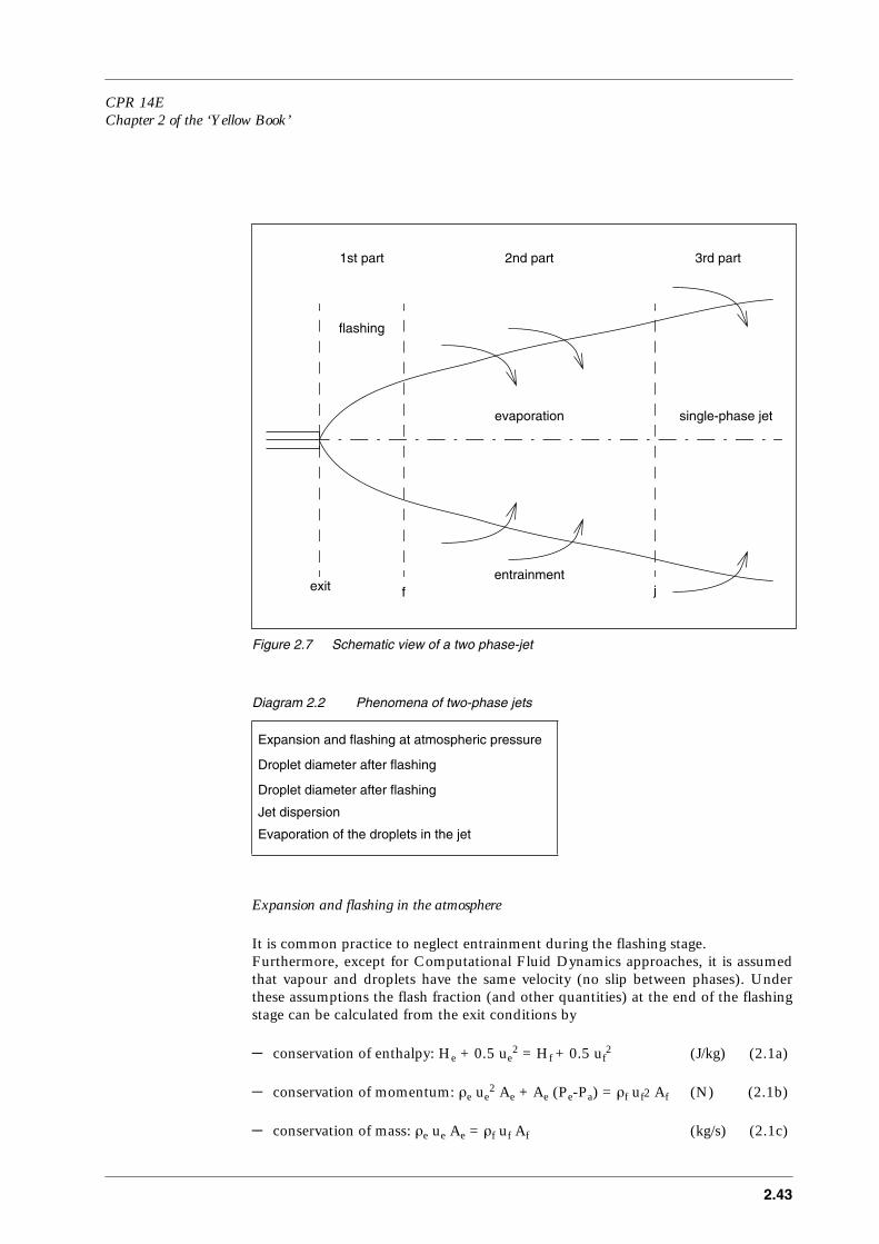
CPR 14EChapter 2 of the ‘Yellow Book’
2.43
Figure 2.7 Schematic view of a two phase-jet
Diagram 2.2 Phenomena of two-phase jets
Expansion and flashing in the atmosphere
It is common practice to neglect entrainment during the flashing stage.Furthermore, except for Computational Fluid Dynamics approaches, it is assumedthat vapour and droplets have the same velocity (no slip between phases). Underthese assumptions the flash fraction (and other quantities) at the end of the flashingstage can be calculated from the exit conditions by
– conservation of enthalpy: He + 0.5 ue2 = Hf + 0.5 uf
2 (J/kg) (2.1a)
– conservation of momentum: ρe ue2 Ae + Ae (Pe-Pa) = ρf uf2 Af (N) (2.1b)
– conservation of mass: ρe ue Ae = ρf uf Af (kg/s) (2.1c)
Expansion and flashing at atmospheric pressure
Droplet diameter after flashing
Droplet diameter after flashing
Jet dispersion
Evaporation of the droplets in the jet
evaporation
entrainment
single-phase jet
flashing
1st part 2nd part 3rd part
exit f j
2.44
– TB is the boiling temperature; Pv˚ (TB) = Pa (N/m2) (2.1d)
– an equation of state relating density to pressure, temperature, and quality. Thevapour density is a function of pressure and temperature (e.g. the perfect gas law),and the density of the liquid phase is a function of temperature alone.
– data on the enthalpies He and Hf as a function of pressure, temperature andquality.
This approach is in principle used in the Yellow Book [1988] and by many otherauthors, e.g. Wheatley [1987]. In his case he used the perfect gas properties and theClausius-Clapeyron relations in order to define the equation of state, the saturationpressure and the enthalpies (assuming isentropic evaporation to give a higher boundon the flash fraction).
Often, e.g. Yellow Book [1988] and Kukkonen [1990], the flash fraction is calculatedusing entropy relations.
In addition to the ‘conventional’ approach described above, some authors, e.g.Woodward [1993], state that equilibrium flash fractions are not established for orificedischarge or short nozzles and pipes. Instead one should use:
Φm,f = CΦmf × Φm,f,equilibrium (-) (2.2)
with
CΦmf = Φm,f,e/0.14 if Φm,f,e ≤ 0.14
CΦmf = 1.0 if Φm,f,e > 0.14
However other authors, e.g. Wheatley [1987], argue that the important parameter inreaching equilibrium is the path length of the flow since nucleation, and this can not,according to Wheatley, be estimated by simple expressions such as those mentionedabove.
Some alternative approaches towards determination of flash fractions and theconditions after flashing can be found. One such an alternative model is presented byWoodward [1993]. This model, which includes determination of critical flow rate,see ‘outflow’, is based on similarity of the two-phase discharge with underexpandedsingle-phase jets. The differences with the ‘conventional’ approach are considerable(higher jet velocities, less diameter expansion). Woodward [1993] states thatexperiments are necessary to decide which of the approaches is better. Another alternative is proposed by Vandroux-Koenig et al. [1991]. They estimate thediameter and velocity after flashing on isotropic increase of bubble size. Also in thatcase the jet velocity is higher and droplet diameters smaller than when using theconventional approach, but the momentum balance is neglected.

CPR 14EChapter 2 of the ‘Yellow Book’
2.45
Droplet diameters after flashing
A liquid jet (either or not flashing) may break-up into droplets due to:– the size of the nozzle (capillary break-up);– aerodynamic break-up of the jet;– shattering by flashing.
For capillary break-up and aerodynamic break-up the literature provides a number ofmodels and descriptions. Most of these descriptions are quite similar, (Tilton &Farley [1990], Wheatley [1987]). The summary of drop size correlations is providedby Tilton and Farley [1990]. This summary includes also correlations for the lengthbefore break-up (relevant to determine which process starts first, e.g. a sub-cooled jetmay break-up aerodynamically before being shattered by flashing, causing largerdrops).
The initial drops formed in the jet may break further by aerodynamic forces. Themaximum stable drop size can be determined using a critical Weber number. Thevalues of critical Weber numbers vary, and may be dependent on parameters notincluded in the Weber number, between 5 and 100, [Wierzba, 1990] but often usedvalues are between 10 and 20 [Tilton & Farley, 1990], Kocamustafaogullari et al.,[1994], Wheatley [1987], Appleton [1984].
Application of the above-mentioned correlations leads to a single number for the dropsize, not allowing for the variation of droplet sizes within a jet. Alternatively,Vandroux-Koenig et al. [1991] suggest assuming a droplet population using an upperlog-normal distribution of which the median is the largest hydro-dynamically stabledrop size.With respect to the effect of shattering, Appleton [1984] and Hague and Pepe [1990]conclude that shattering of the jet by flashing occurs if the exit temperature exceedsa ‘shatter’ temperature Tsh, which obeys
(-) (2.3)
Here TB is the boiling temperature and Cε is 0.07 - 0.1 (Appleton) or 0.1 (Hague andPepe).Estimates of drop size due to shattering are provided by Tilton & Farley [1990],Appleton [1984] and Vandroux-Koenig [1991]. The approach used by Vandroux-Koenig et al. [1991] requires an estimate of the rate of depressurisation in the flashingjet, which is not easy to obtain.
Most authors however, determine the drop size after flashing by using the criticalWeber number for aerodynamical break-up. In this way effects of coalescence ofdroplets (droplet growth) do not have to be dealt with separately and the methodexplains the experimental (low) fractions of rain-out satisfactorily.
Droplet evaporation and rain-out on the ground
Droplets will settle by gravity and they can fall on the ground, forming an(evaporating) pool.
Tsh TB–
Tsh-------------------- Cε=

2.46
The calculation of the trajectory of droplets is generally performed by assuming thatthe horizontal velocity of the droplet equals the horizontal jet velocity, and the verticalvelocity (settling velocity) follows from the aerodynamic drag force. The evaporation of droplets has been given much attention in recent research. In viewof differences in complexity, one has to distinguish between1. evaporation of a pure, single component droplet,2. evaporation of a binary (or multi) component droplet.The first approach is more simple and leads to more analytic or simple definiteconclusions.A simple approximate expression for the droplet diameter dm for which drying timeand settling time to the ground are equal, has been derived by Kukkonen et al.[1989]. Only droplets larger than dm will fall on the ground. Expressions describingthe change of droplet mass up to the moment the droplet falls on the ground can bederived using the basic model principles.The same principles are used by Papadourakis et al. [1991] and Woodward &Papadourakis [1991]. Droplet evaporation is combined with calculations of thedroplet trajectory in differential form. The calculations are combined with an integralplume trajectory model, and the difference between jet trajectory and droplettrajectory defines the ‘ambient’ droplet conditions for evaporation and drag. Allevaporated chemical is fed ‘back’ into the jet/plume model.
The evaporation of binary component droplets is described by Vesala [1990], Vesala& Kukkonen [1992] and Pattison [1992].Pattison attempts to include the binary component model in a jet/plume model framework comparable to Woodward & Papadourakis [1991] as described above, see alsoHewitt & Pattison [1992]. This leads to an extensive set of coupled ordinarydifferential equations.
In order to obtain some information about the relevance of the binary componentmodel compared to the single component droplet evaporation model, the evolutionof droplets was investigated by Vesala and Kukkonen [1992]: in 100% humid air, 20˚C ambient temperature, initial diameter 100 µm, the ‘drying’ time of a binaryammonia/water droplet is reduced by a factor 1.5 compared to a single componentammonia droplet in dry air (and thus ignoring ‘binary’ effects).
Jet dispersion
A droplet-laden two-phase jet is assumed to behave like a pure vapour jet. Accordingto Wheatley [1987], Kukkonen [1990], Webber et al. [1991], entrainment ratesidentical to those for pure vapour jets can be used. The jet model allows for predictionthe change of concentration, velocity and radius of the jet along the jet axis. Thefollowing section will address droplet evaporation in the jet.
Evaporation of the droplets in the jet
The rate of evaporation of droplets in the jet is dominated by the amount of entrainedair and the amount of heat brought into the jet by the entrained air. The calculationof droplet evaporation in the jet can be made by the enthalpy balance at any point inthe jet.

CPR 14EChapter 2 of the ‘Yellow Book’
2.47
A rigorous derivation of concentration, phase balance and enthalpy balance indifferential form, i.e. changes in properties related to small increases of entrained airin the jet, is provided by Webber et al. [1991]. Webber considers differentpossibilities: 1. Two-phase chemical dispersing in dry air.2. Two-phase chemical which is immiscible with water dispersing in moist air.3. Two-phase chemical which forms an ideal solution in water (i.e. the partial vapour
fraction of the chemical is linear to the molar fraction of chemical solved in water)dispersing in moist air.
4. NH3 dispersing in moist air.5. HF dispersing in moist air.
However, it is not always necessary to use a differential approach. In some cases it ispossible to make use of enthalpy- and phase balances at arbitrary positions in the jetwithout needing to solve differential equations. Examples of these methods areprovided by Kukkonen [1990], who treats the 2nd possibility from above, Wheatley[1987] (possibility 4), and Webber and Brighton [1989] (possibilities 2 to 4).
The latter calculate the temperature after entrainment by evaluating the enthalpychanges when a certain amount of moist air at Ta is mixed with chemical at flashingconditions (Xf, TB). The nett change of enthalpy is zero:
0 = ∆H = ∆Hchemical + ∆Hdry air + ∆Hwater vapour (J/kg) (2.4)
The individual enthalpy changes include the temperature change, both of liquid andvapour, and the heat of evaporation and/or condensation.If the chemical is soluble in water, the scheme remains the same, but the liquid phasewill be mixed. It also means that in most cases, if the chemical does not form an idealsolution in water, an additional term ∆Hmixing has to be added to the enthalpy balanceabove to account for the fact that chemicals dissolving in water produce heat (e.g.ammonia). Also the saturated vapour pressures of both water and chemical changeand become dependent on the mixture fraction in the droplet.Methods to calculate the mixing enthalpy and saturation pressures forammonia/water mixtures are provided on an empirical way by Wheatley [1987] andin a more general way by Vesala & Kukkonen [1992] If one is only interested in the situation at cross-section ‘j’ after complete evaporationof the chemicals, the nett mixing enthalpy equals zero.
The above-described approach assumes liquid and vapour to have the sametemperature, and no velocity difference between the phases. This is the so called‘homogeneous equilibrium’ theory (HE). According to Kukkonen [1990], atemperature difference, i.e. the ‘temperature depression’, is necessary to driveevaporation. By comparison with advanced models, Kukkonen [1993] concludes thatat least in clouds, HE theory can be used for droplets up to 100 µm. It is notnecessarily valid in the jet region where high entrainment occurs. Furthermore, itappeared that the results were not very sensitive to the thermodynamic properties, i.e.the differences between Wheatley’s [1990] and Vesala & Kukkonen’s [1992]expression.
2.48
2.3.4.7 Instantaneous releases pressurised liquefied gases
Statement of the problem
This section considers the release following a complete failure of a vessel containingliquefied gases stored under pressure at a temperature above normal boiling point.After failure, the liquid will flash and expand in all directions until the vapour/liquidmixture is cooled below boiling point.After flashing, the cloud will expand further and entrain ambient air. The entrainedair will cause further evaporation of liquid droplets in the cloud. Part of the dropletsmay fall on the ground and form an evaporating pool.For consequence analysis it is necessary to be able to describe the evolution of thecloud size and the concentration in the cloud after the release, before atmosphericdispersion takes over, and the fraction of the release that remains in the air comparedto the fraction that will form an evaporating liquid pool.In order to describe the evolution of the instantaneous release, separate descriptionsor models are needed for the following phenomena taking place in the expanding two-phase cloud:– the flashing of the liquid phase after release, leading to the vapour mass fraction
and temperature in the two-phase cloud; – the evolution of the size, expansion velocity and concentration of the two-phase
cloud;– the fraction deposited of liquid droplets on the ground (rain-out fraction);– the evaporation of droplets in the two-phase cloud due to air entrainment and the
thermodynamic state (temperature, density) of the mixture.
A division in three stages, similar to that used for continuous releases, can be made.First, the liquid flashes and expands without entrainment. Secondly, air is entrained,droplets may rain-out and/or evaporate due to entrained air. Finally all chemicaldroplets disappear and a single-phase cloud remains.
Again, emphasis will be on the first two stages. The phenomena are also summarisedin Diagram 2.3. The first two boxes refer to the first stage, the last two boxes to thesecond stage. Models and descriptions of the phenomena in Diagram 2.3 arediscussed in the following sections. A number of methodologies described in section2.3.4.6 (continuous releases) will also be applicable to instantaneous releases.
Diagram 2.3 Phenomena of instantaneous releases of pressurisedliquefied gases
Flashing and initial cloud expansion
Droplet size and rain-out on the ground
Expansion of the two-phase cloud during the entrainment phase
Evaporation of the droplets in the cloud

CPR 14EChapter 2 of the ‘Yellow Book’
2.49
The study of instantaneous releases is far less developed than the study of continuous(jet) releases. The largest scale experiments reported are those by British Gas[Johnson et al., 1990], involving a commercial storage vessel of 5.7 m3 filled with 2tonnes of butane (fill ratio 77% by volume). For this test only visual and LIDAR-dataof the expanding cloud is available.Other rather large-scale experiments are those of Hardee and Lee [1975] regarding450 kg of welding gas ‘MAPP’ and propane, and Giesbrecht et al. [1981] involving435 kg of propylene.Small-scale tests have been performed using refrigerants (Nolan et al. [1991] 1 litre,Schmidli et al. [1992] 2 litres, and HSE, Webber et al. [1991] 20 litres) and propane(Schmidli et al. [1992] 2 litres).With respect to the use and importance of small-scale experiments, Nolan et al.[1991] point out that a rigorous analysis of scaling aspects is necessary, but has notas yet been performed, in order to translate small-scale experiments to reality.Especially the rain-out behaviour of small-scale experiments is difficult to extrapolateto large-scale, and the older large-scale experiments provide no information on rain-out.
Flashing and initial cloud expansion
For the flashing stage immediately after the loss of containment it is reasonable toassume that no ambient air will entrain into the cloud, Webber et al. [1991].The conditions in the cloud just after complete flashing can be described by theenthalpy balance, taking into account the kinetic energy of the expanding cloud andthe work performed on the atmosphere [Melhem & Croce, 1993], [Nolan et al.,1991]:
H0 = Φm,f HV,f + (1-Φm,f) HL,f + 0.5 uf2 + (P0 - Pa)/ρ0 (J/kg) (2.5)
In order to calculate the unknown flash fraction Φm,f and the expansion velocity uf,the thermodynamic path between H0 and Hf needs to be known. Assuming anisentropic evaporation, an upper boundary for uf and a lower boundary for Φm,f canbe obtained.From experiments [Nolan et al., 1991], [Schmidli et al., 1992], [Webber et al., 1991]it is obvious that the expansion velocity is smaller than it would be by assumingisentropic evaporation and using the above mentioned enthalpy balance, but thedifferences in results and conclusions are large. Some researchers [Schmidli et al.,1992], [Webber et al., 1991] find expansion velocities of only 10% - 30% of thetheoretical, isentropic values. However the data from Nolan et al. [1991] leads toexpansion velocities which are about 60% - 80% of the theoretical, isentropic values(see also the analysis of Nolan et al.’s data by Melhem and Croce [1993]).The reasons for lower-than-theory expansion velocities are that part of the kineticenergy is transformed into turbulent kinetic energy, the evaporation and expansionprocess is not isentropic and during the flashing stage no equilibrium state is reached(Webber et al. [1991] describe non-equilibrium between temperature and pressureduring the HSE-experiments).Nevertheless, no simple relation between ‘theoretical’ and real expansion velocitiescan be derived.

2.50
Droplet size and rain-out on the ground
In order to estimate the possibility of liquid rain-out on the ground there is an interestin describing the droplet size in the aerosol cloud after flashing.Measurement and analysis of droplet size are reported by Nolan et al. [1991] andSchmidli et al. [1992]. Observed droplet sizes are (much) smaller than the maximumstable droplet diameter, using a critical Weber-number and the expansion velocity ofthe cloud (cf. section 2.3.4.6). No other droplet size theories have been published.
No physically sound models have been found to describe rain-out and dropletevaporation in instantaneous releases. The settling of aerosols depends on the height to which droplets are carried, and therate at which ambient air is mixed in the cloud in order to evaporate the droplet. It isreasonable to assume a dependence on the size of the release for droplet settling.Moreover, rain-out occurs not only by settling of aerosol in the cloud, but also byimpingement of droplets by the energy of the expanding cloud in the early stages ofexpansion.
Cavanaugh et al. [1994] suggest the assumption that all liquid will be emitted asaerosol if the storage temperature exceeds the boiling temperature by 10 K. Forboiling temperatures between 200-250 K, this corresponds to a ‘shattering’ criterion(see formula (2.3), section 2.3.4.6) in which Cε is less than 0.05. However,Cavanaugh’s assumption is supported neither by physical reasoning nor experimentaldata.
Only Schmidli et al. [1992] provide quantified experimental information on theamount of rain-out and pool formation for Refrigerants 12 and 114. Even for releasesexceeding the ‘shattering’ criterion with Cε=0.1, a significant amount of mass remainsin the pool. Impact of liquid on the ground during the early stage of expansion seemsto be the major cause. A reduced liquid fill level leads to increased pool formation asthe vapour above the liquid forces the liquid downwards during expansion.It is common practice to assume that twice the amount of the flashing liquid remainsairborne. This assumption provides a rough but reasonable approximation of theresult of Schmidli et al. Of course, such a simple rule does not account for probabledependency of rain-out on droplet diameter, release size or fill level.
Expansion of the aerosol cloud during the entrainment phase
No generally accepted model for the expansion of an instantaneous aerosol cloudexists. The models published by Giesbrecht et al. [1981] and Hardee & Lee [1975]for the expansion after flashing are very different in their approach. The model included in the Yellow Book [1988] and the ‘Worldbank’ model are basedon the work by Giesbrecht et al. [1981]. Webber et al. [1991], however, criticize theYellow Book [1988] model as it fails to reproduce the HSE experiments.The model by Hardee & Lee [1975] for the expansion rate of the cloud is based onconservation of momentum, but they assume no expansion in vertical direction, andthe release is not purely instantaneous, but a large puncture in a vessel.The simplest approach, using Hardee & Lee’s ideas, is to assume that during flashingthe expansion velocity is constant and that it can be calculated using formula (2.5),possibly with a correction for non-isentropy and turbulence. Afterwards an expandingcloud with a uniform concentration is assumed. The momentum which is contained
CPR 14EChapter 2 of the ‘Yellow Book’
2.51
in a segment of the (hemi-) spherical cloud at the moment when flashing is complete,will be conserved. From this and from neglecting the density difference between thecloud and the ambient air, one derives the uniform radial velocity in the cloud, whichis also assumed to be the expansion velocity:
u(t) = uf (bf/b(t))3 (m/s) (2.6)
Here, bf is the cloud radius at the moment when flashing is complete, and b the cloudradius at any moment thereafter. By stating u = db/dt, one can derive the evolutionof the cloud size with time.The expansion rate according to this simple model agrees fairly well with theexperimental results of Giesbrecht et al. [1981], assuming expansion in ahemispherical cloud at ground level. The model applies until the expansion velocity is of the same magnitude as theambient wind speed.
Evaporation of the droplets in the cloud
All statements made in section 2.3.4.6 for droplet evaporation in continuous releasesare applicable to the expanding aerosol cloud. No research is known towards theapplicability of the HE-assumptions for instantaneous clouds. In the later stage of thecloud, the expansion velocities become small and the HE approach may probably beapplied.
2.3.5 Liquids
The models for (non-boiling) liquids neglect the vapour pressure of theliquid, being not higher than atmospheric.Non-boiling liquids are liquids that have a normal boiling point higher than theambient temperature, or refrigerated liquefied gases at (nearly) atmospheric pressure.
2.3.5.1 Introduction to liquids
In general the hydraulic pressure of the liquid is the driving force of a flowof a non-boiling liquid out of a vessel. In case a liquid has been pressurised, the hydraulic pressure may be much smallerthan the storage pressure, and the effect of the decreasing liquid level may benegligible. This is also true if pressurised liquefied gas has been set under pressurehigher than the saturated vapour pressure.
The flow of liquids in orifices and in pipes, and the rather simple behaviour of liquidin a vessel, have been well established for many years. In the previous edition of the[YellowBook, 1988] models for liquid outflow through holes have been given, and sohave laminar and turbulent flows of fluids in pipes (i.e. gases ánd liquids).

2.52
2.3.5.2 Vessel dynamics liquids
Applying the basic law of conservation of mass, and taking into account thehydraulic pressure of a liquid column, will suffice for an adequate description of thevessel dynamics.The hydraulic pressure determining the mass flow rate depends on the liquid level inthe tank. The only slightly complicating factor may be the estimation of the liquidlevel as function of the filling degree and geometry of the vessel. For simplegeometries (sphere, cylinders) relations hL=F(VL) exist.
2.3.5.3 Liquid flow through holes and piping
Well-known relations for the stationary outflow through orifices andthrough pipes exist. In the previous edition [YellowBook, 1988] models for laminarand turbulent flow of fluids have been given. More details can be found in section 2.5.
Simple analytical expressions exist for predicting the outflow rate through small holesin the vessel wall (punctures), as functions of time, in case the vessel has a simplegeometric form. In Foster [1981], Lee [1987], Woodward [1991], Crowl [1993] andSommerveld [1993], analytical expressions are inferred to compute the time it takesto empty vessels of different shapes: vertical cylinders, cone, horizontal cylinders,spheres, and other. In Hart [1993], equations are given to estimate liquid dischargeamounts and rates from a flow opening at any arbitrary elevation. In figure 2.8 someexamples of these models have been given.
Figure 2.8 Time required to empty a vessel [Foster, 1981]
CPR 14EChapter 2 of the ‘Yellow Book’
2.53
2.3.5.4 Non-stationary liquid flow in pipelines
No model has been found in open literature except the model in theprevious edition of the [YellowBook, 1988]. This model is an approximate solutionof the mass balance (continuity equation) and the momentum balance governing theliquid flow in a horizontal pipeline. It has been assumed that after the full borerupture of the pipeline, a decompression wave is travelling upstream into the pipe.The liquid flow is assumed to be stationary between this upstream moving wave andthe downstream pipe end.
The average isothermal compressibility of liquids between 1 and 1000 bar (105-108 N/m2) is about:
β = 1.0 × 10⁻⁹ m2/N
with
β = - 1/V × (∂V/∂P)T (2.7)
This means that with pipe pressure below 200-300 bar (2-3 × 10⁷ N/m2), the liquidvolume has been compressed to a volume which is only a few percent smaller.Due to the minor compressibility of liquids in general, it is advised to set the massflow rate equal to the pump flow rate in case of a full bore rupture, taking into accountless friction due to a smaller pipe length until the breakage. In case of a relatively smallhole in the pipe wall, the outflow rate may be based on the initial pressure in thepipeline.
2.3.6 Friction factors
Friction factors have been given in the previous edition [YellowBook,1988]. Additional information can be found in, for instance Melhem [1993] andRadford [1990].The models for outflow through pipes have been developed for a pipe with no bends,reductions of cross-section or branches. If such fittings are present, they can beaccounted for by introducing either an equivalent pipe length or extra resistancecoefficients. In section 2.5 we put them together.
2.3.7 Physical properties of chemicals
Fluid flow and the vaporisation of liquids are controlled by thermodynamiclaws and laws governing physical transport phenomena. Relations for thermophysicalproperties have been given for well-known commodities in many publications.
2.54
Pressure, volume, temperature (PVT) relationships for gases and liquids, and alsosolids would preferably all be summarised in the form of equations of state of thegeneral type:
v = f(P,T) (m3/mol) (2.8)
where
v = specific volume [m3/mol]P = absolute pressure [N/m2]T = absolute temperature [K]
In theory it is possible to derive the thermodynamic properties from an equation ofstate, like:
Tfl = flash point [K]Cp = specific heat [J/(kg⋅K)]ρ = liquid density [kg/m3]P˚ = vapour pressure [N/m2]H = enthalpy [J/kg]S = entropy [J/(kg⋅K)]Lv = heat of vaporisation [J/kg]
Only in the case of gases there has been much progress in the development of thesestate equations. They are obtained by correlation of empirical PVT data, and alsofrom theoretical considerations based on atomic and molecular structure. Theequation of state of gases will be addressed in more detail in section 2.5.
For compressible chemicals, gases and two-phase mixtures with vapour, the densitydepends strongly on pressure and temperature.The physical properties of condensate phases, liquefied gases, liquids and solids, aswell as the other physical properties of gases do not vary much as a function ofpressure P at moderate pressures, and may be expressed as functions of temperatureonly. Temperature-dependent thermodynamic and physical transport properties ofpure chemicals will be addressed in the annex to this Yellow Book.
Multi-component systems that act as a multi-phase system at given pressure,temperature and composition will not be addressed because they demand specifictreatment. Mono-phase multi-component mixtures can be treated as quasi one-componentsystems only in case of ideal mixing, meaning using average values for the physicalproperties proportional to the weight fractions of the chemical in the mixture.

CPR 14EChapter 2 of the ‘Yellow Book’
2.55
2.4 Selection of models
2.4.1 Introduction to section 2.4
In section 2.4 the considerations which have led to the selection of themodels that are included in section 2.5, are explained. In section 2.5 these models willbe described in detail. In general the selection is based on the followingconsiderations.
Safety studies and hazard assessment require models that are reasonably accurate,demand little computational effort and not too much input. Larger computational demands of the model are acceptable only if the accuracy of thepredictions will be much greater and/or when the model has a (much) wider range ofapplicability.Needless complicated models that mainly make an additional scientific contributionshould be avoided, yet we must not close our eyes to future developments.
Leaving all models relying on computational fluid dynamics (CFD) behind, two mainpractical approaches may be distinguished:
1. Simple models, such as approximating analytical expressions and empiricalcorrelations, meant for predictions of maximum and averaged flow rates andduration of the outflow.
2. Numerical procedures without approximating sub-models, meant for predictionsof the outflow rate as function of time.
The analytical equations may be used to get a quick estimate of the magnitude of theoutflow rate. These models are based on simplifying assumptions like: perfect gasbehaviour, constant physical properties, and unchanged boundary conditions.A numerical approach takes into account changes of the physical properties as afunction of temperature and pressure, non-perfect gas and liquid behaviour, and‘sudden’ changes in boundary conditions.
The (specific) considerations that have lead to the selection of the models to bedescribed in section 2.5, are presented as follows:– sub-section 2.4.2 addresses models for gases;– sub-section 2.4.3 addresses models for releases of pressurised liquefied gases,
including spray releases;– sub-section 2.4.4 addresses models for releases of (non-boiling) liquids.
2.4.2 Gases
The well-known relations for the stationary critical and non-critical outflowof gases through orifices and through pipes are as in the previous edition of theYellowBook [1988].
2.56
There is not much discussion about applying standard thermodynamics for thedescription of vessel dynamics, as will be described in section 2.5. We have opted for numerical models, because these models are still relatively simple,and are able to cope with varying physical properties and sudden changes inconstraints.
The model for non-stationary gas flow in pipelines in the previous edition of the[YellowBook, 1988] was not validated, has a bad performance, and seemsnumerically unsound. The Wilson correlation has good performance and is rathersimple [Hanna, 1987]. This model will be described in section 2.5.
The Weiss correlation [Weiss, 1988] for small holes in pipelines is the only modelfound in open literature. Therefore it will be described in chapter 2.5.
No model to cope with crater formation, in case of leaks from buried pipelines, ispublicly available, therefore no model can be included in section 2.5.
Vapour outflow
The models for outflow of gas through holes and piping are valid for pure vapourflowing out of the vapour section in the containment for vaporising pressurisedliquefied gases.
2.4.3 Pressurised liquefied gases
2.4.3.1 Vessel dynamics pressurised liquefied gases
The depressurising of a pressurised liquefied gas causes bubble formationin the liquid and thus expansion of the boiling liquid is a rather complexphenomenon.A large computer model has been given in Haque [1992].Because other models are much more complex and obviously do not have a (much)better performance, it would be advisable to use the Fauske correlation to determinewhether there exists a two-phase flow inside the vessel or not [Fauske, 1988]. Thismodel is simple and based on experimental data for horizontal cylinders and spheres.In Melhem [1993] a refined DIERS-method has been described that distinguishesdifferent ways of boiling for top venting and relations to estimate the quality in theoutflow opening for vertical vessels. In Sheppard [1993] it appears that this analyticalsolution of the DIERS-method validates the Fauske correlation, but this analyticalsolution is also able to predict disengagement, regardless of vessel shape. So the DIERS-method is to be preferred, being more generally applicable and notmuch more complicated. In chapter 2.5 the analytical DIERS-method is described.
A comparison of the results of both models in Haque [1992] shows that thecorrelation of Mayinger [Belore, 1986] may well be used for the estimation of the voidfraction in relatively small vessels. The present state of knowledge about the effects ofbulk liquid sub-cooling on mitigating the liquid swell, permits only case by casenumerical solutions involving sizeable computer programs [Sallet, 1990,3].
CPR 14EChapter 2 of the ‘Yellow Book’
2.57
Therefore, due to lack of a better and also manageable model, it is advised to applythe correlation of Mayinger, also for larger vessels.
The fact that the void fraction in the top of the vessel venting may be much higherthan the average value, can only be coped with by applying very complicated models.Although the behaviour of a depressurising pressurised liquefied gas is a complexprocess, we choose to describe a model based on standard thermodynamics, takinginto account the criteria of DIERS and Mayinger. We have opted for a numerical model, instead of analytical solutions, because thesemodels are still relatively simple, but are able to cope with varying physical propertiesand sudden changes in constraints, predicted by the criteria of DIERS and Mayinger.This approach will be described in section 2.5.
2.4.3.2 Stationary outflow of vapour through holes and piping
The well-known relations for the stationary critical and non-critical outflowof gases through orifices and through pipes are valid for one-phase vapour flow, andwill be described in section 2.5.
2.4.3.3 Two-phase outflow through holes and piping
Giot et al. have carried out a benchmark on two-phase-flow models, withinthe European Union program ‘Major Technological Hazards’, on the basis ofselected well-documented and reliable data sets [Giot, 1992].The benchmark has led to the conclusion that most models presented in openliterature have a limited validity range.The main conclusions are:1. Only Flinta’s model has a acceptable performance on all ranges,2. ‘Homogeneous Equilibrium Models’ (HEMs) generally underpredict.However, a very limited number of data points related to fluids other than water wereincluded in the database and have been used for model validation [Giot,1992].
The TPDIS-model has been selected because of:1. HEM is broadly accepted, and according to Giot [1996] HEMs will give
reasonable predictions if the quality φm,e is larger than 1%,2. TPDIS is a complete model, well-described in open literature.
Flinta’s model has not been selected because of:1. Its general applicability has not been proven,2. Some quantities in the required formulae cannot be easily obtained or derived.
It is advised to use TPDIS and other HEMs for those situations for which they havebeen validated.

2.58
2.4.3.4 Non-stationary two-phase flow in pipelines
Having presumably a low accuracy and a not very robust numerical solutionprocedure, and not being validated, any simpler and validated model is to bepreferred to the previous Yellow Book model.
A generally applicable model is necessary. Therefore the model given in Morrow[1983] will be described in section 2.5. This model has been derived for propane, butcould be generalised by using appropriate physical properties.
While propane is often transported in pipelines, the specific correlation given in Tam[1990] will also be described in this section.
2.4.3.5 Finite duration spray releases
Expansion and flashing at atmospheric pressure
The selected model to calculate the conditions after flashing is based on theconventional, generally accepted model using the equations (2.1a-d) provided insection 2. No correction is applied for non-equilibrium flash fractions because of lackof consensus on this subject.
Droplet diameter after flashing
The proposed model for initial droplet size is based on the work by Appleton [1984]and presented by Wheatley [1987]. These expressions are relatively simple to use andAppleton [1984] compared the proposed dropsize correlations with availableexperimental data. He concludes (for his case, a water/steam mixture at 192 ˚C,0.8 mm orifice) that there is reasonable agreement between the correlations andexperimental data.The correlations are different for shattered and non-shattered jets. The criterion forshattering follows the suggestions by Appleton with Cε = 0.1.
Droplet evaporation and rain-out on the ground
The proposed methodology to predict droplet rain-out from a two-phase jet is:1. To refrain from the description of binary droplet evaporation in view of
uncertainty in exit droplet size and the moderate reductions in drying timesaccording to Vesala [1990];
2. First to determine whether droplets at the end of the flashing zone will reach theground using Kukkonen’s [1990] limiting radius;
3. If the droplets in the jet exceed the limiting droplet radius, then calculate theevaporated mass fraction until the droplet hits the ground. The deposited massfraction is subtracted from the liquid mass entering the vapour jet, and will forman evaporating pool. For these evaporation calculations, use is made of theexpressions by Kukkonen [1990] assuming evaporation in pure air. Only velocitydifferences between droplet and air due to settling are considered, the horizontalvelocity of the jet and the droplet are assumed to be the same.
CPR 14EChapter 2 of the ‘Yellow Book’
2.59
Jet dispersion
It is assumed that the two-phase jet after flashing can be treated as a single-phase jetwith respect to width, entrainment, and evolution of concentration and velocity onthe jet centre line. This leads to the conclusion that the single-phase vapour jet model as described inchapter 4 is applicable, using the jet diameter after flashing as the exit condition.
Evaporation of the droplets in the jet
The evaporation of droplets remaining in the jet due to the heat brought into the jetby entrained air is relevant to determine the density of the jet. In order to calculatethe conditions in the jet after evaporation of the aerosols, use will be made of thehomogeneous equilibrium model. It has been demonstrated that the homogeneousequilibrium model may be used for droplets less than 100 µm in clouds. The essenceof the homogeneous equilibrium method is the use of the integral balance for theenthalpy in the jet (2.4) in section 2.3.4.6, and neglecting temperature differencesbetween the two-phases.
2.4.3.6 Instantaneous release of pressurised liquefied gas
Flashing and initial cloud expansion
The flash fraction is calculated assuming isentropic flashing. The expansion velocityis calculated using the enthalpy balance (2.5), but multiplied by 0.8 to account forturbulence and non-isentropy. This factor is justified by the available experimentaldata.
Expansion of the aerosol cloud during the entrainment phase
For the evolution of cloud size the simple model as presented in section 2.3.4.7 isselected because there is no evidence that more complex and advanced modelsprovide better results compared to the scarce data. The concentration in the cloud isassumed to be uniform.
Droplet size and rain-out on the ground
By absence of alternatives and considering an instantaneous airborne vapour cloud togive conservative results, it is assumed that a total mass of twice the isentropic flashfraction (in addition to the initial vapour mass in storage) will remain airborne.This simple model makes no use of droplet diameter, so no model for calculating thedroplet diameter after flashing has been selected.

2.60
Evaporation of the droplets in the cloud
The conditions in the cloud at the moment when all aerosols have evaporated, arecalculated by using exactly the same methods as included in the two-phase jet model(section 2.3.4.6).The self-driven expansion of the cloud is assumed to have ended when all aerosolshave evaporated and the expansion velocity is equal to the ambient wind speed at theheight of the initially expanded cloud just before entrainment starts.
2.4.4 Liquids
Since there is not much discussion about which models to apply for liquidflow through holes and pipes, and the behaviour of liquid vessels, the standardapproach will be followed in section 2.5.
Most analytical models for liquid vessel dynamics suffice, although the expressionsare not always simple to calculate and integral tables might be needed. We have optedfor numerical models for the description of vessel dynamics in order to be able tomaintain the same approach as in the previous paragraphs.
A specific model for non-stationary liquid flow in pipelines is not considered relevant.
CPR 14EChapter 2 of the ‘Yellow Book’
2.61
2.5 Description of models
2.5.1 Introduction to section 2.5
Section 2.5 provides descriptions of the recommended models for releasesof compressed gases, pressurised liquefied gases and (non-boiling) liquids.It contains all necessary information to perform the calculations. For background ofthe models the reader may refer to section 2.3.Section 2.5 provides detailed descriptions of the models and methods for thefollowing releases:– subsection 2.5.2 addresses models for releases of gases;– subsection 2.5.3 addresses models for releases of pressurised liquefied gases,
including spray releases;– subsection 2.5.4 addresses models for releases of non-boiling liquids.Finally, friction factors for pipe flow will be given in subsection 2.5.5.
Guide to the calculations
First, the reader must determine the state of the chemical in its containment, bymeans of the criteria given in subsection 2.2.3 and summarised in the diagram 2.4.
Diagram 2.4 Thermodynamic states
Secondly, the reader should check the failure mode of the containment.
Thermodynamic state Physical conditions
I. compressed gas T > Tc or P < Pv˚(T)
II. pressurised liquefied gas P = Pv˚(T)
III. (non-boiling) liquid Tm < T < TB(P)
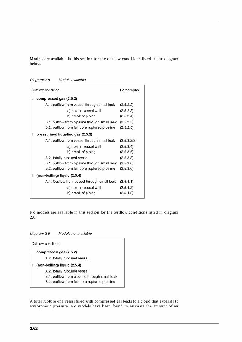
2.62
Models are available in this section for the outflow conditions listed in the diagrambelow.
Diagram 2.5 Models available
No models are available in this section for the outflow conditions listed in diagram2.6.
Diagram 2.6 Models not available
A total rupture of a vessel filled with compressed gas leads to a cloud that expands toatmospheric pressure. No models have been found to estimate the amount of air
Outflow condition Paragraphs
I. compressed gas (2.5.2)
A.1. outflow from vessel through small leak (2.5.2.2)
a) hole in vessel wall (2.5.2.3)b) break of piping (2.5.2.4)
B.1. outflow from pipeline through small leak (2.5.2.5)B.2. outflow from full bore ruptured pipeline (2.5.2.5)
II. pressurised liquefied gas (2.5.3)
A.1. outflow from vessel through small leak (2.5.3.2/3)
a) hole in vessel wall (2.5.3.4)b) break of piping (2.5.3.5)
A.2. totally ruptured vessel (2.5.3.8)B.1. outflow from pipeline through small leak (2.5.3.6)B.2. outflow from full bore ruptured pipeline (2.5.3.6)
III. (non-boiling) liquid (2.5.4)
A.1. Outflow from vessel through small leak (2.5.4.1)
a) hole in vessel wall (2.5.4.2)b) break of piping (2.5.4.2)
Outflow condition
I. compressed gas (2.5.2)
A.2. totally ruptured vessel
III. (non-boiling) liquid (2.5.4)
A.2. totally ruptured vesselB.1. outflow from pipeline through small leakB.2. outflow from full bore ruptured pipeline

CPR 14EChapter 2 of the ‘Yellow Book’
2.63
entrained during the expansion. Most atmospheric dispersion models assume that theinitial cloud has not been diluted.
A total rupture of a vessel filled with non-boiling liquid leads to a spreading pool onthe ground or on a water surface. The release phenomena are taken into account inthese pool spreading models.
In section 2.4.4 arguments were given for not describing models for (long) liquidpipelines. The equations given in subsection 2.5.4.2 may be used.
2.5.2 Compressed gases
2.5.2.1 Equation of state for gases
Because gases are compressible, the gas density ρ(P) as a function of the gaspressure P must be known.The equation of state of a perfect gas is given by:
P × V = n × R × T (J) (2.9a)
or
v = R × T/(P × µi) (m3/kg) (2.9b)
note that
v = 1/ρ (2.9c)
where
P = absolute gas pressure [N/m2]T = absolute temperature [K]R = gas constant [J/(mol⋅K)]n = number of moles [-]v = specific volume [m3/kg]V = volume [m3]µi = mol mass of gaseous chemical i [kg/mol]ρ = density [kg/m3]
The perfect gas equation describes the PVT behaviour of real gases only to a firstapproximation.
A way of showing the deviations from ideality is to write for the real gas:
P × V = z × n × R × T (J) (2.10a)
or
v = z × R × T/(P × µi) (m3/kg) (2.10b)

2.64
where
z = compressibility factor [-]
The factor z is called compressibility factor, although this might be confusing becausethe factor z has no relation with the compressibility of a gas. The German term‘Realgasfaktor’ is more plain [Gasunie, 1980]; the factor z expresses the departurefrom the perfect gas behaviour with one single factor.
The compressibility factor appears to be a universal function of the so-called reducedtemperature and pressure:
z = f(PR,TR) (-) (2.11)
with
PR = P/Pc (-) (2.11a)
TR = T/Tc (-) (2.11b)
where
PR = reduced pressure [-]Pc = critical pressure of the chemical [N/m2]TR = reduced temperature [-]Tc = critical temperature of the chemical [K]
Figure 2.9 Compressibility factor as function of reduced state variables by Gouq-Jen Su [Moore, 1972]
For perfect gases the compressibility factor z equals unity. It is noted that mostdeviation from perfect gas behaviour occurs near the thermodynamic critical pressure

CPR 14EChapter 2 of the ‘Yellow Book’
2.65
and critical temperature. In general for real gases the compressibility factor z is aboutunity for high temperature and low pressures.
Other classical equations of state for real gases are those by Van der Waals andBerthelot. The Van der Waals equation [Moore,1972] may be expressed as:
(PR + 3/VR2) × (VR-1/3) = 8/3 × TR (2.11c)
with
VR = V/Vc (-) (2.11d)
and
Vc = 3/8 × R × Tc/Pc (m3/mol) (2.11e)
where
Vc = critical volume [m3/mol]VR = reduced volume [-]
In Leung [1988] the Redlich-Kwong-equation of state for gases has been used. Also viral equations may be used to represent the behaviour of gases with greateraccuracy, having more adjustable coefficients.The Starling-Han equation and chemical dependent coefficients have been presentedin [Edminster, 1984]. In Morrow’s model the Starling equation is used, seeparagraph 2.5.3.6.
2.5.2.2 Vessel dynamics compressed gas
The modelling of the dynamics of compressed gas stored in a vessel aims atpredicting the decrease of pressure and temperature due to the outflow of gas.Due to the release of gas the remaining gas in the vessel will expand. This expansioncauses cooling and depressurisation.
The model is basically an iterative numerical procedure in which the outflow of gasout of a vessel is described in small steps. These steps should be small enough toconsider the conditions in the vessel to be constant during one time-step.First, the initial condition and termination condition of the numerical procedure willbe given. After this the model in the form of a numerical procedure is given. Thisnumerical procedure has to be repeated until the termination conditions will havebeen satisfied.Afterwards, the inference is given of the system equation governing the behaviour ofthe compressed gas in the vessel used in the model.
The initial and termination condition of the numerical procedure concerning gas outflow
The initial condition of the vessel is given by: P1, T1, ρ1, meaning i=1.The duration of δt may freely be chosen in principle, and depends of the number of

2.66
time-steps Nt. When one wishes to estimate the mass flow rate and vessel conditionsat time tend, then the size of time step δt is given by
δt = tend/Nt (s) (2.12)
t = time from the start of the outflow [s]
The larger the number of steps, the higher the accuracy of the model, but the moretime needed for the calculation. The choice Nt=50 will be appropriate for mostcalculations.
The numerical procedures given should be repeated as long as the constraints arevalid:
ti < tend P > Pa T > Tm (2.13)
The model for gas outflow: a numerical procedure
Starting every step at time ti in the iteration with a condition in the vessel given by Pi,Ti, ρi, the following procedure aims at calculation of the condition in the vessel at theend of the small time-step δt, given by Pi+1, Ti+1, ρi+1.
Let us say that the outflow rate qS,i is given by a generalised function f, depending onwhether the outflow is through a hole (see paragraph 2.5.2.3) or a pipe (see paragraph2.5.2.4)
qS,i = f(Pi,Ti,ρi,...) (kg/s) (2.14)
Due to the gas release in period δt, the density in the vessel decreases
δρ = - qS,i/V × δt (kg/m3) (2.15)
ρi+1 = ρi + δρ (kg/m3) (2.16)
ti+1 = t + δt (s) (2.17)
These steps should be small enough to consider the conditions in the vessel to beconstant during one time-step.
Due to the decrease of the gas density, the gas will expand and the gas temperaturewill decrease; applying the system equation (see Intermezzo below) gives
δT = Pi/( × Cv) × δρ (K) (2.18)
Ti+1 = Ti + δT (K) (2.19)
The change in density and temperature of the gas forces the pressure to adapt to thenew conditions according to the equation of state of (non-perfect) gases given byequation (2.10b)
ρi2

CPR 14EChapter 2 of the ‘Yellow Book’
2.67
Pi+1 = z × ρi+1 × R × Ti+1/µj (N/m2) (2.20)
with
z = z(PR,i,TR,i) (-) (2.21)
The new condition of the vessel at time ti+1 given by: Pi+1, Ti+1, ρi+1.As long as the termination condition has not been fulfilled, this procedure has to berepeated.
Intermezzo: inference of the system equation (2.18) for compressed gases
The equations without a reference number in this paragraph are only part of the inference of the systemequation that is required.Applying the first law of thermodynamics and using the definition of volumetric work done by anexpanding gas, gives
∆U = QH - ∫ P × dv (J/kg) (2.18a)
where
∆U = change in internal energy of the gas [J/kg]P = gas pressure [N/m2]v = specific volume of the gas [m3/kg]QH = heat transferred into 1 kg gas [J/kg]
Note that the internal energy U is given per unit mass in the vessel.
Assuming reversible adiabatic outflow results in
δU = P × δV (J/kg) (2.18b)
δX = small change in quantity X
Neglecting the internal pressure of non-perfect gases gives a relationship between the internal energy of gasand its temperature
δU = Cv(T) × δT (J/kg) (2.18c)
Cv = specific heat at constant volume the gas [J/(kg.K)]
Using the definition of density ρ and combining the equations leads to the system equation that governsthe behaviour of the gas in the vessel, namely
Cv × δT = P/ρ2 × δρ (J/kg) (2.18d)
ρ = density [kg/m3]
2.5.2.3 Gas outflow through holes
The modelling of the outflow of gas through holes aims at predicting themass flow rate as a function of pressure drop over the hole.
The mass flow rate for gas outflow through an orifice can be estimated by ageneralised equation
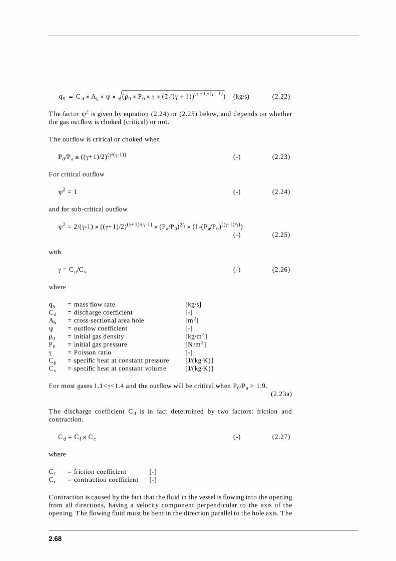
2.68
(kg/s) (2.22)
The factor ψ2 is given by equation (2.24) or (2.25) below, and depends on whetherthe gas outflow is choked (critical) or not.
The outflow is critical or choked when
P0/Pa ≥ ((γ+1)/2)(γ/(γ-1)) (-) (2.23)
For critical outflow
ψ2 = 1 (-) (2.24)
and for sub-critical outflow
ψ2 = 2/(γ-1) × ((γ+1)/2)(γ+1)/(γ-1) × (Pa/P0)2/γ × (1-(Pa/P0)((γ-1)/γ))(-) (2.25)
with
γ = Cp/Cv (-) (2.26)
where
qS = mass flow rate [kg/s]Cd = discharge coefficient [-]Ah = cross-sectional area hole [m2]ψ = outflow coefficient [-]ρ0 = initial gas density [kg/m3]P0 = initial gas pressure [N/m2]γ = Poisson ratio [-]Cp = specific heat at constant pressure [J/(kg⋅K)]Cv = specific heat at constant volume [J/(kg⋅K)]
For most gases 1.1<γ<1.4 and the outflow will be critical when P0/Pa > 1.9.(2.23a)
The discharge coefficient Cd is in fact determined by two factors: friction andcontraction.
Cd = Cf × Cc (-) (2.27)
where
Cf = friction coefficient [-]Cc = contraction coefficient [-]
Contraction is caused by the fact that the fluid in the vessel is flowing into the openingfrom all directions, having a velocity component perpendicular to the axis of theopening. The flowing fluid must be bent in the direction parallel to the hole axis. The
qS Cd A× h ψ ρ0 P0 γ 2 γ 1+( )⁄( ) γ 1+( )/ γ 1–( )×××( )××=

CPR 14EChapter 2 of the ‘Yellow Book’
2.69
inertia of the fluid results in the smallest cross-sectional area, with no radialacceleration, that is smaller than the area of the opening.For sharp orifices contraction plays a part and friction is negligible;The following value for the discharge coefficient is recommended [Beek, 1974]:
Cd ≈ 0.62 (2.28a)
For rounded orifices contraction does not play a part and friction is small;The following value for the discharge coefficient is recommended [Beek, 1974]:
Cd ≈ 0.95 - 0.99 (2.28b)
Vapour outflow
The models for outflow of gas from holes are valid for pure vapour flowing out of thevapour section in the containment for vaporising pressurised liquefied gases, as longas no condensation of the vapour occurs. This means that the pressure of the vapourmay not become higher than its saturation pressure at given temperature.
2.5.2.4 Gas outflow through piping
The modelling of the outflow of gas through piping aims at predicting themass flow rate as a function of the pressure drop over the piping. This mass flow rateis mainly determined by the overpressure in the vessel and the flow resistance.
Principles of the model for gas flow in piping
The total pressure drop ∆P between the vessel and the ambient is equal to thepressure drop over the pipe and the pressure drop over the downstream opening inthe pipe
∆P = P0 - Pa (N/m2) (2.29a)
= (P0 - Pe) - (Pe - Pa)
= ∆Ppipe - ∆Phole
with
∆Phole = Pe - Pa (N/m2) (2.29b)
∆Ppipe = P0 - Pe (N/m2) (2.29c)
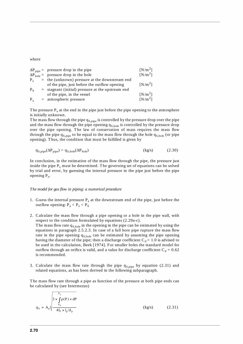
2.70
where
∆Ppipe = pressure drop in the pipe [N/m2]∆Phole = pressure drop in the hole [N/m2]Pe = the (unknown) pressure at the downstream end
of the pipe, just before the outflow opening [N/m2]P0 = stagnant (initial) pressure at the upstream end
of the pipe, in the vessel [N/m2]Pa = atmospheric pressure [N/m2]
The pressure Pe at the end in the pipe just before the pipe opening to the atmosphereis initially unknown. The mass flow through the pipe qS,pipe is controlled by the pressure drop over the pipeand the mass flow through the pipe opening qS,hole is controlled by the pressure dropover the pipe opening. The law of conservation of mass requires the mass flowthrough the pipe qS,pipe to be equal to the mass flow through the hole qS,hole (or pipeopening). Thus, the condition that must be fulfilled is given by
qS,pipe(∆Ppipe) = qS,hole(∆Phole) (kg/s) (2.30)
In conclusion, in the estimation of the mass flow through the pipe, the pressure justinside the pipe Pe must be determined. The governing set of equations can be solvedby trial and error, by guessing the internal pressure in the pipe just before the pipeopening Pe.
The model for gas flow in piping: a numerical procedure
1. Guess the internal pressure Pe at the downstream end of the pipe, just before theoutflow opening: Pa < Pe < P0
2. Calculate the mass flow through a pipe opening or a hole in the pipe wall, withrespect to the condition formulated by equations (2.29a-c).The mass flow rate qS,hole in the opening in the pipe can be estimated by using theequations in paragraph 2.5.2.3. In case of a full bore pipe rupture the mass flowrate in the pipe opening qS,hole can be estimated by assuming the pipe openinghaving the diameter of the pipe; then a discharge coefficient Cd = 1.0 is advised tobe used in the calculation, Beek [1974]. For smaller holes the standard model foroutflow through an orifice is valid, and a value for discharge coefficient Cd = 0.62is recommended.
3. Calculate the mass flow rate through the pipe qS,pipe by equation (2.31) andrelated equations, as has been derived in the following subparagraph.
The mass flow rate through a pipe as function of the pressure at both pipe ends canbe calculated by (see Intermezzo)
(kg/s) (2.31)qS Ap
2 ρ P( ) dP×P0
Pe
∫×
4fF lp/dp×-----------------------------------=

CPR 14EChapter 2 of the ‘Yellow Book’
2.71
with
ρ = C × (P/z)1/ζ (kg/m3) (2.32)
ζ = 1 + z × R/(Cv × µi) (-) (2.33)
where
C = constant
Note that for perfect gas behaviour (z=1)
ζ = γ (-) (2.33b)
The integral may be solved simply by numerical methods, but also analyticallyassuming constant compressibility factor, for instance z = 1, and constant specificheat at constant volume Cv:
(kg2/(m4⋅s2))(2.31a)
4. Compare those two mass flow rates qS(∆Ppipe) and qS(∆Phole). If not equal repeatprocedure.
A more convenient way to solve equation (2.30) is to use a root finding procedure bydefining
F(Pe) = qS,pipe(∆Ppipe) - qS,hole(∆Phole) (kg/s)
= qS,pipe(P0-Pe) - qS,hole(Pe-Pa) (kg/s) (2.30a)
The principle is still the same, but the determination of the right Pe is much quicker.
Intermezzo: inference of the equation (2.31) describing the mass flow rate of gas flow in a pipe
The total pressure drop for a stationary fluid flow (gases and fluids) in piping can be estimated by the well-known Darcy-Weisbach equation
∆P = fD × ρg/2 × ug2 × lp/dp (N/m2) (2.198a)
This relation does not account for the effect of the pressure drop on the density of the gas, whichconsequently will expand. In the following the equation will be inferred which relates the mass flow rate qS
of a gas in a pipe to the pressure drop in the pipe. Reformulated for the local pressure drop along the pipethe relation gives
δP/δlp = fD × ρg/2 × ug2/dp (N/m3) (2.198b)
ρ P( )P0
PE
∫ dP Po ρo ζ 1 ζ+( )⁄( )××≈× Pe Po⁄( ) 1 ζ+( ) ζ⁄( ) 1–( )×
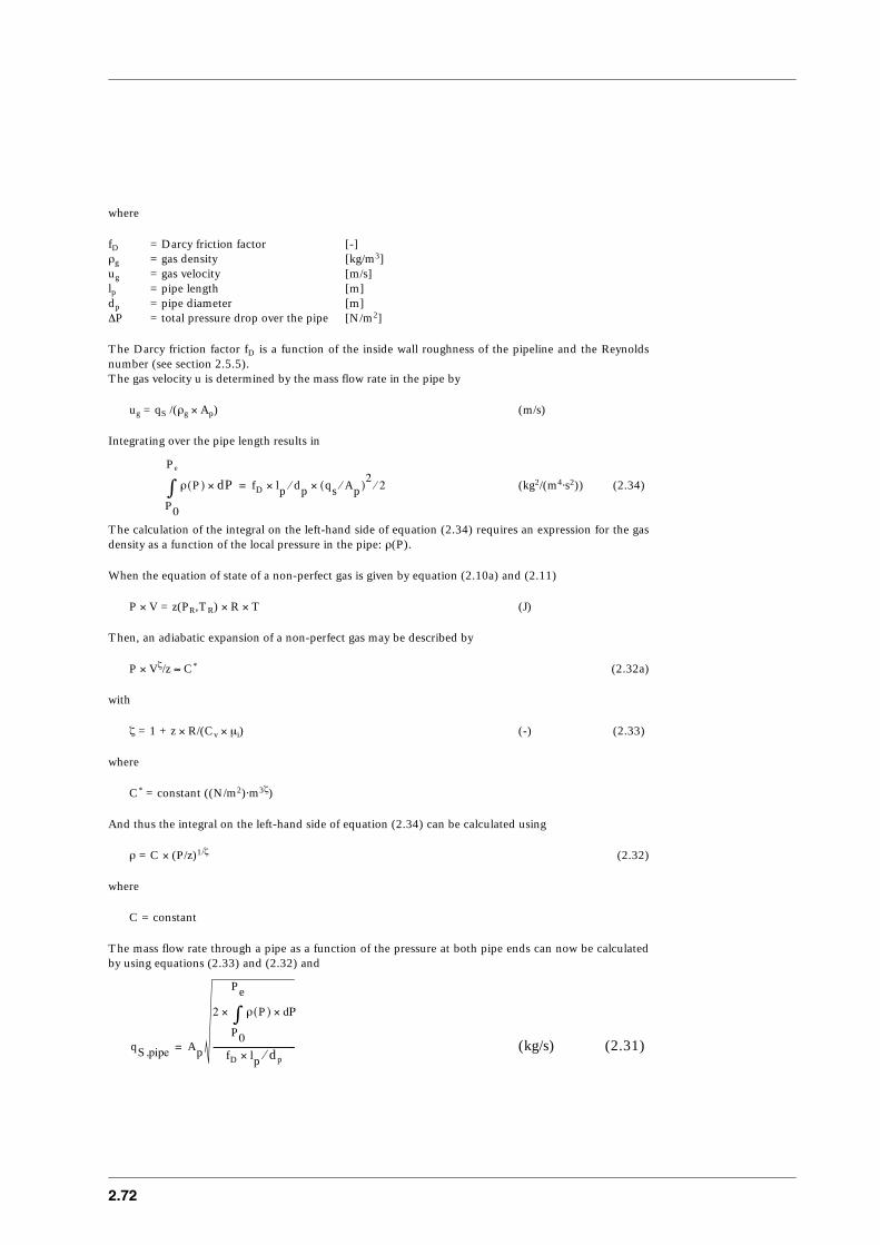
2.72
where
fD = Darcy friction factor [-]ρg = gas density [kg/m3]ug = gas velocity [m/s]lp = pipe length [m]dp = pipe diameter [m]∆P = total pressure drop over the pipe [N/m2]
The Darcy friction factor fD is a function of the inside wall roughness of the pipeline and the Reynoldsnumber (see section 2.5.5).The gas velocity u is determined by the mass flow rate in the pipe by
ug = qS /(ρg × Ap) (m/s)
Integrating over the pipe length results in
(kg2/(m4⋅s2)) (2.34)
The calculation of the integral on the left-hand side of equation (2.34) requires an expression for the gasdensity as a function of the local pressure in the pipe: ρ(P).
When the equation of state of a non-perfect gas is given by equation (2.10a) and (2.11)
P × V = z(PR,TR) × R × T (J)
Then, an adiabatic expansion of a non-perfect gas may be described by
P × Vζ/z ≈ C* (2.32a)
with
ζ = 1 + z × R/(Cv × µi) (-) (2.33)
where
C* = constant ((N/m2)⋅m3ζ)
And thus the integral on the left-hand side of equation (2.34) can be calculated using
ρ = C × (P/z)1/ζ (2.32)
where
C = constant
The mass flow rate through a pipe as a function of the pressure at both pipe ends can now be calculatedby using equations (2.33) and (2.32) and
(kg/s) (2.31)
ρ P( ) Pd×
P0
Pe
∫ fD lp dp qs Ap⁄( )2
2⁄×⁄×=
qS ,pipe Ap
2 ρ P( ) dP×
P0
Pe
∫×
fD lp× dp⁄--------------------------------------=
CPR 14EChapter 2 of the ‘Yellow Book’
2.73
Vapour outflow
The models for outflow of gas through piping are valid for pure vapour flowing out ofthe vapour section in the containment for vaporising pressurised liquefied gases, aslong as no condensation of the vapour occurs. This means the pressure of the vapourmay not become higher than its saturation pressure at given temperature.
2.5.2.5 Non-stationary gas flow in pipelines
After a sudden rupture at one end of the pipeline, a pressure wave will startmoving with the speed of sound in the pipeline in the opposite (upstream) direction.
Non-stationary gas flow in pipelines after a full bore rupture
The Wilson model of the outflow of gas through pipelines aims at predicting the massflow rate as a function of time depending on the initial conditions. The model assumes a compressor to trip when the decompression wave in thepipeline reaches the compressor station at the other pipe end.
The mass flow rate for a full bore ruptured pipeline according to the empirical modelof Wilson [Hanna, 1987] is given by
qS(t) = qS,0/(1+Q0/(tB × qS,0))×Q0/(tB × qS,0) × exp(-t/tB)+exp(-t × tB × (qS,0/Q0)2)(kg/s) (2.35)
where
qS,0 = initial mass flow (discharge) rate [kg/s]Q0 = initial total gas mass in the pipeline [kg]tB = time constant [s]
1. The initial total mass Q0 in the pipeline can be calculated by
Q0 = ρ0 × Ap × lp (kg) (2.36a)
with
Ap = π/4 × dp2 (m2) (2.36b)
2. The initial release rate qS,0 can be calculated by using the equations presented inparagraph 2.5.2.4
(kg/s) (2.37)
For outflow through the pipe opening in case of a full bore rupture it is advised to usethe following value for the discharge coefficient
Cd = 1.0 (-) (2.38)
qS ,0 Cd Ap ψ ρ0 P0 γ 2 γ 1+( )⁄( ) γ 1+( ) γ 1–( )⁄×××( )×××=
2.74
3. The sonic velocity in the gas us, assuming adiabatic expansion (∆S=0) is given by
us = √(dP/dρ)s (m/s) (2.39a)
Using the equations of state for non-perfect gases given in paragraph 2.5.2.4 results in
dρ/dP = ρ/(ζ × P) (s2/m2) (2.39b)
which results for non-perfect gases in
(m/s) (2.39c)
4. The Darcy friction factor may be calculated by the Colebrook-White equation,approximated for high Reynolds numbers, by
fD = 1/(-2 × 10log(ε/(3.715 × dp)) 2 (-) (2.40)
5. The time constant tB is given by
(s) (2.41)
6. Finally the mass flow rate qS(t) can be estimated at any time t after the full borerupture of the pipeline by the Wilson model given by equation (2.35).
7. Check the validity of the model.When the pressure wave travelling upstream reaches the opposite side of thepipeline the Wilson model is not valid any more. This is the case when
tE = lp/us (s) (2.42)
The following symbols used in this paragraph have not been mentioned earlier:
dp = pipe diameter [m]lp = pipe length [m]Q0 = initial mass content in the pipeline [kg]P0 = initial (operating) pressure in pipeline [N/m2]qS,0 = initial mass flow (discharge) rate [kg/s]T0 = initial temperature [K]t = time after rupture [s]tE = maximum time validity model [s]fD = Darcy friction factor [-]γ = specific heat ratio [-]ε = wall roughness [m]ζ = constant defined paragraph 2.5.2.4 [-]µi = molecular weight of substance i [kg/mol]ρ = density of the gas [kg/m3]ρ0 = initial density of the gas [kg/m3]
us ζ z R T0 µi⁄×××( )=
tB 2 3 lρ×⁄ us⁄ γ fD lρ dρ⁄××( )×=

CPR 14EChapter 2 of the ‘Yellow Book’
2.75
Non-stationary gas outflow from pipelines through small holes
The Weiss model of the outflow of gas from pipelines through punctures (small holes)aims at the estimation of the blow-down time (and not the mass flow rate as a functionof time).The model has been developed for blow-down riser design, but can be applied to asmall hole in a pipeline similarly.
The method for accurately predicting gas-pipeline blow-down times, involvesapplication of appropriate correction factors to a simple calculation that regards thepipeline as a volume. The correction factors apply to a wide range of length/diametervalues and the ratio of the main pipe area to the area of the small holes [Weiss, 1988].It is assumed that the gas within the pipeline expands isothermally.The effect of friction in the pipeline can have pronounced effects on the blow-downtime. The cross-area of a small hole is much smaller than the cross-section of thepipeline. Consequently the gas velocities in the pipeline are moderate and the flowmay be regarded as quasi-steady. In case the (fD × lp/dp)<40 the pipeline may beconsidered as a stagnant volume neglecting the effects of flow and friction in thepipeline.An attempt was made to formulate correction factors which could be applied to thevolume model calculations in order to provide better blow-time predictions.The result was a polynomial expression in (fD × lp/dp) and pipe to hole area(Ap/Ah⋅Cd)Note that the Darcy friction factor fD is explained in subsection 2.5.5.
Numerical procedure non-stationary blow-down time of pipelines through small holes
1. Determine the average speed of sound us and the Poisson ratio γ for the blow-down and calculate the time constant τv
τv = Vp × (s) (2.43)
(m/s) (2.44)
(m3) (2.45)
γ = Cp/Cv (-) (2.26)
2. Calculate the dimensionless sonic blow-down time
τcr = ln(Pi/Pa) - (γ/(γ-1)) × ln((γ+1)/2) (-) (2.46)
3. Calculate the dimensionless sub-sonic blow-down time τs by solving the followingequation by a standard numerical integration procedure (method by Simpson orRomberg)
(-) (2.47a)
γ 1+( )/2( ) γ 1+( )/ 2 γ 1–( )( )
us Ah Cd××-----------------------------------------------------
us z γ R T µi⁄×××( )=
Vpπ4---
dp2 lp××=
τs21/ γ 1–( ) γ 1–( )×
γ 1+( ) γ 1–( )/ 2 γ 1–( )×( )----------------------------------------------1
p p 2/γ– p γ 1+( )/γ––( )×------------------------------------------------
Pcr
Pf
∫×= dp×
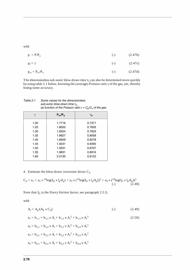
2.76
with
p = P/Pa (-) (2.47b)
pf = 1 (-) (2.47c)
pcr = Pcr/Pa (-) (2.47d)
The dimensionless sub-sonic blow-down time τs can also be determined more quicklyby using table 2.1 below, knowing the (average) Poisson ratio γ of the gas, yet, therebylosing some accuracy.
Table 2.1 Some values for the dimensionless sub-sonic blow-down time τs as function of the Poisson ratio γ = Cp/Cv of the gas
4. Estimate the blow-down correction factor Cb
Cb = a1 + a2 × 10log(fD × lp/dp) + a3 × (10log(fD × lp/dp))2 + a4 × (10log(fD × lp/dp))3
(-) (2.48)
Note that fD is the Darcy friction factor; see paragraph 2.5.5;
with
Ar = Ap/(Ah × Cd) (-) (2.49)
a1 = b1,1 + b1,2 × Ar + b1,3 × Ar2 + b1,4 × Ar
3 (2.50)
a2 = b2,1 + b2,2 × Ar + b2,3 × Ar2 + b2,4 × Ar
3
a3 = b3,1 + b3,2 × Ar + b3,3 × Ar2 + b3,4 × Ar
3
a4 = b4,1 + b4,2 × Ar + b4,3 × Ar2 + b4,4 × Ar
3
γ Pcr/Pa τs
1.20 1.7716 0.7371 1.25 1.8020 0.7605 1.30 1.8324 0.7833 1.35 1.8627 0.8058 1.40 1.8929 0.8278 1.45 1.9231 0.8495 1.50 1.9531 0.8707 1.55 1.9831 0.8916 1.60 2.0130 0.9122
CPR 14EChapter 2 of the ‘Yellow Book’
2.77
These coefficients have been matched with a numerical pipe model that correspondswell with experimental data.
(2.51)
b1,1 = 0.88107 b1,2 = -0.064749 b1,3 = 0.0067921 b1,4 = -0.00019302
b2,1 = 0.82784 b2,2 = 0.053443 b2,3 =-0.0088474 b2,4 = 0.00026646
b3,1 =-0.78302 b3,2 = -0.0086017 b3,3 = 0.0049027 b3,4 = -0.00016658
b4,1 = 0.34043 b4,2 = -0.032399 b4,3 = 0.0013735 b4,4 = -0.000023546
These correlations are valid for
4 ≤ Ar ≤ 16 (2.52)
The following correlations
a1 = c1,1 + c1,2 × (1/Ar) + c1,3 × (1/Ar)2 + c1,4 × (1/Ar)
3 (2.53)
a2 = c2,1 + c2,2 × (1/Ar) + c2,3 × (1/Ar)2 + c2,4 × (1/Ar)
3
a3 = c3,1 + c3,2 × (1/Ar) + c3,3 × (1/Ar)2 + c3,4 × (1/Ar)
3
a4 = c4,1 + c4,2 × (1/Ar) + c4,3 × (1/Ar)2 + c4,4 × (1/Ar)
3
with
c1,1 = 1.0319 c1,2 = -5.2735 c1,3 = 25.680 c1,4 = -38.409 (2.54)
c2,1 =-0.26994 c2,2 = 17.304 c2,3 =-86.415 c2,4 = 144.77
c3,1 = 0.24175 c3,2 =-12.637 c3,3 = 56.772 c3,4 = -88.351
c4,1 =-0.054856 c4,2 = 2.6258 c4,3 = -8.9593 c4,4 = 12.139
apply to a somewhat wider validity range
3 ≤ Ar ≤ 30 (2.55)
but may be not so good a fit in the middle range, and can best be used at theextremities of the range
3 ≤ Ar < 4 (2.56)
16 ≤ Ar ≤ 30

2.78
5. The duration of the outflow can be determined by
t = (τcr+τs) × τv × Cb (s) (2.57)
The following symbols have been used in this paragraph:
Ap = cross-sectional area pipeline [m2]Ah = cross-sectional area hole [m2]Cd = discharge coefficient hole [-]Cb = blow-down correction factor [-]dp = pipeline diameter [m]fD = Darcy friction factor [-]γ = Poisson ratio [-]lp = pipe length [m]P = (absolute) pressure [N/m2]p = pressure ratio (P/Pa) [-]pcr = critical flow pressure ratio [-]pf = final pressure ratio [-]Pa = atmospheric pressure [N/m2]P0 = initial pipeline pressure [N/m2]R = gas constant [J/(mol⋅K)]T = absolute temperature [K]τcr = dimensionless sonic blow time [-]τs = dimensionless subsonic blow time [-]us = speed of sound [m/s]V = pipeline volume [m3]z = compressibility factor [-]ρ = density [kg/m3]τv = time constant [s]
2.5.3 Pressurised liquefied gases
2.5.3.1 Introduction to pressurised liquefied gases
The modelling of the dynamics of a vessel filled with pressurised liquefiedgas aims at predicting the decrease in temperature and liquid mass during outflow.
The way the content in the vessel behaves (‘vessel dynamics’) is very much dependenton the type of outflow initially from the vessel:* outflow of pure vapour Φm = 1* two-phase outflow 0 < Φm< 1* liquid outflow Φm = 0Note that Φm is the quality or vapour mass fraction of the outflowing fluid.
In order to determine which flow type will be at hand, the swell of the boiling liquiddue to the bubble formation relative to the position of the opening inside the vesselshould be estimated first. The DIERS-criteria determine whether two-phase flow

CPR 14EChapter 2 of the ‘Yellow Book’
2.79
inside the vessel is apparent in case of top venting. In case of a release the rise of theliquid level can be estimated by the relation of Mayinger [Belore, 1986].
The model is basically an iterative numerical procedure in which the outflow of gasand liquid from a vessel is described in small steps. These steps should be smallenough to consider the conditions in the vessel to be constant during one time-step.
The outlines of the numerical procedure for the vessel dynamics concerning therelease of pressurised liquefied gas is somewhat different for each flow type.The procedure corresponding to the vessel dynamics resulting from outflow of purevapour (Φm=1) will be described first. The other procedures will be described as avariant of this procedure.
In the following, first the criteria for the flow type inside the vessel and the model forliquid level rise are given.Next, the initial and termination condition of the numerical procedure will be given. After this the model in the form of a numerical procedure is described. Every flowtype is related to its own variant of the basic procedure.The numerical procedure has to be repeated until the termination conditions willhave been satisfied, and as long as the initial flow type remains.
2.5.3.2 Determination outflow type from the vessel
Flow type inside the vessel
A detailed analytical method for predicting the flow regime for two-phase flows froma vertical vessel during depressurisation was developed by the Design Institute ofEmergency Relief Systems (DIERS) of the American Institute of Chemical Engineers(AIChE) [DIERS, 1986 and Melhem, 1993].
The DIERS-method proceeds as follows:
1. Determine the outflow rate qs,1, assuming vapour outflow at the exit, by using theequations presented in paragraphs 2.5.2.3 and 2.5.2.4.
2. Calculate the superficial vapour velocity inside the vessel
uV = qs,1 /(ρV × AL) (m/s) (2.58)
3. Calculate the bubble rise velocity
ub = CD1 × (g × σ × (ρL - ρV))0.25/√ρL (m/s) (2.59)
with
CD1 = 1.18 for bubbly flow (-) (2.60a)
CD1 = 1.53 for churn flow (extensive bubble coalescence) (-) (2.60b)
σ = surface tension (N/m) (2.60c)

2.80
In figure 2.3 (page 2.24) the bubble flow region and the churn turbulent flow regionhave been outlined.
4. The dimensionless superficial vapour velocity is given by
uVR = uV/ub (-) (2.61)
5. Calculate the characteristic dimensionless superficial velocity uVR for both typicaltwo-phase flow types.
For bubbly flow the dimensionless superficial velocity uVR must be greater than
uVR,bf = Φv × (1 - Φv)2/((1 - Φ3
v) × (1 - CD2 × Φv)) (-) (2.62a)
with
CD2 = 1.2 for bubbly flow (2.62b)
For churn flow the dimensionless superficial velocity must be greater than
uVR,cf = 2 × Φv/(1 - CD2 × Φv) (-) (2.62c)
with
CD2 = 1.5 for churn flow (2.62d)
The average void fraction Φv,av in the vessel is assumed to be given by
Φv,av = 1 - φ (m3/m3) (2.63)
6. Determination whether two-phase flow is apparent inside the vessel, if so than twophase outflow occurs.
Application of the criteria
uVR ≥ uVR,cf → two-phase churn flow (-) (2.64a)
uVR ≥ uVR,bf → two-phase bubbly flow (-) (2.64b)
uVR < uVR,bf and uVR < uVR,cf → vapour outflow (-) (2.64c)
Note that if both conditions (2.64a) and (2.64b) are satisfied that churn flow prevails.
If condition (2.64b) is satisfied while two-phase flow is in progress, disengagement ispredicted.
CPR 14EChapter 2 of the ‘Yellow Book’
2.81
7. If vapour outflow is predicted, then the procedure is finished. If two-phase flow ispredicted, the quality for top venting Φm,e,2 can be estimated by an implicitfunction
(-) (2.65)
The parameters fΦv1 and fΦv2 are flow dependent.For bubbly flow:
(-) (2.65a)
and
(-) (2.65b)
For churn flow:
(-) (2.65c)
and
(-) (2.65d)
Note: use the correct value for CD2.
Equation (2.65) has to be solved iteratively.
The outflow rate qs,2 in every iteration step, must be recalculated by the equations inparagraph 2.5.3.4 or 2.5.3.5, taking quality φm,e,2 into account.
WhereAL = vessel cross sectional area [m2]ub = bubble rise velocity [m/s]uV = superficial vapour velocity in vessel [m/s]uVR = dimensionless superficial velocity [-]uVR,bf = minimum dimensionless superficial [-]
velocity for bubbly flow uVR,cf = minimum dimensionless superficial [-]
velocity for churn flow φ = filling degree of vessel [m3/m3]Φm,e = quality (mass fraction vapour) at the exit [kg/kg]Φv,av = average void fraction in the vessel [m3/m3]
φm,e,2 qs ,2×
fΦv1 fΦv2 ub ρv AL××××----------------------------------------------------------
1
1 CD2 fΦv1× ρv/ρL( ) 1 φm,e,2–( )/φm,e,2××–----------------------------------------------------------------------------------------------------=
fΦv1 Φv av, 1 CD2– Φv av,×( )⁄=
fΦv2 1 Φv av,–( )2/ 1 Φv av,3–( )=
fΦv1 2 Φv av,× / 1 CD2 Φv av,×–( )=
fΦv2 1=
2.82
Rise liquid level
After a (sudden) depressurisation the liquid in the vessel will flash, and due to thepresence of vapour bubbles in the tank the liquid will expand, necessitating aredefinition of liquid height.The correlation of Mayinger [Belore, 1986] may be used for the estimation of the voidfraction in the liquid phase in vessels. The procedure may also be used to determinethe rise of the liquid level for outflow through the side wall of the vessel, in order tocheck if two-phase outflow will occur.
The void fraction or hold-up in a flashing liquid due to depressurisation is calculatedusing the following procedure [Belore,1986].
The superficial vapour velocity is given by
uV,0 = qS/(ρV × AL) (m/s) (2.58)
The surface tension at boiling point, may be calculated using Walden’s rule [Perry,1973]:
σ = Cσ × Lv(ΤΒ) × ρL (N/m) (2.66)
with
Cσ = 6.56 × 10⁻⁷ m
The ratio of the liquid kinematic viscosity to the gas kinematic viscosity at boilingpoint can be calculated by using Arrhenius’s relation for liquid viscosity [Perry, 1973]and Arnold’s correlation for gas viscosity [Perry, 1973], resulting in
υL/υV = CAA × (µi × 103)1/6 × ρV × (T+1.47 × TB) / (ρL7/6 × T3/2) (-) (2.67)
with
CAA = 37 [m-1/2⋅kmol1/6 K1/2]
For convenience we define
(m) (2.68a)
The void fraction is given by
Φv = 0.73 × (uV,02/(g × CΦv))
0.376 × (CΦv/dv)0.176 × (ρL/(ρL-ρV))0.585 × (υL/υV)0.256
(m3/m3)(2.68b)
The liquid with bubbles will expand to a new volume
VL,E = VL,0/(1-Φv) (m3) (2.69)
Cφv σ g ρL ρV–( )×( )⁄=

CPR 14EChapter 2 of the ‘Yellow Book’
2.83
The increased liquid height can be estimated by using the inverse function betweenliquid volume and liquid height for the specific geometry of the vessel (see paragraph2.5.4.1), written in generalised form
hL,i = F-1(VL,i) (m) (2.70)
Where
Φv = void fraction [m3/m3]qS = discharge rate [kg/s]AL = normal liquid surface in the vessel [m2]dv = vessel diameter [m]T = liquid/vapour temperature [K]µi = mol weight chemical i [kg/mol]ρL = liquid density [kg/m3]ρV = vapour density [kg/m3]Lv(ΤΒ) = heat of vaporisation at boiling point [J/kg]TB = normal boiling point [K]uV,0 = superficial vapour velocity [m/s]σ = surface tension [N/m]g = gravitational acceleration [m/s2]υL = liquid kinematic viscosity [m2/s]υV = vapour kinematic viscosity [m2/s]VL,E = expanded ‘liquid’ volume in the vessel [m3]VL,0 = initial liquid volume in the vessel [m3]
2.5.3.3 Vessel dynamics related to outflow type
The initial and termination conditions for all type of outflows from vessel filled withpressurised liquefied gas
The initial condition of the vessel (i=1) is given by its temperature T1, filling degreeφ, and vessel volume V.The initial vapour mass QV,1 and liquid mass QL,1 in the vessel can easily be derived,given the filling degree φ and the storage temperature, by
QL,1 = φ × V × ρL,1 (kg) (2.71)
QV,1 = (1-φ) × V × ρV,1 (kg) (2.72)
with
ρL,1 = ρL(T1)
ρV,1 = ρV(T1)
The duration of δt may be chosen freely in principle, and depends of the number oftime-steps Nt. When one wishes to estimate the mass flow rate and vessel conditionsat time tend, then the size of time step δt is given by
2.84
δt = tend/Nt (s) (2.12)
t = time from the start of the outflow [s]
The larger the number of steps, the higher the accuracy of the model, but the moretime needed for the calculation. The choice Nt=50 will be appropriate for mostcalculations.The numerical procedures given should be repeated as long as the constraints arevalid, namely
ti < tend P > Pa T > Tm (2.73a)
In case of liquid outflow, an additional constraint for the liquid level is active, namely
hL > hhole (2.73b)
Every time-step the criteria of DIERS and Mayinger should be checked. During theblow-down the amount of liquid may decrease so that the swelled liquid level willdrop and pure vapour outflow may become apparent again eventually. In case of topventing the churn flow may change into bubbly flow, or the two-phase flow maydisengage.
If the flow type changes during the outflow, then we have to switch to the appropriatevessel dynamics model. The calculation restarts with the vessel conditions at themoment of the switch.
1. Vessel dynamics pure vapour outflow (quality Φm=1)
This version of modelling of the dynamics of a vessel with pressurised liquefied gasaims at predicting the decrease in temperature and liquid mass during outflow of onlyvapour. The vessel dynamics are mainly controlled by the evaporation of thepressurised liquefied gas, which is assumed to be at saturated vapour pressureinitially.
In case no two-phase flow is apparent inside the vessel when top venting, or the riseof the expanded liquid is below the hole in the vessel wall, only vapour outflow willbe at hand. Due to the outflow of vapour the vessel depressurises. This causes theliquefied gas to evaporate, and subsequently the temperature will decrease and so willthe saturated vapour pressure.The basic assumptions of the model are:1. Liquid mass is removed by evaporation only.2. The vapour phase is in thermodynamic equilibrium with its liquid phase, which
means that the actual vapour pressure is equal to the saturated vapour pressure atliquid temperature.
3. The heat capacity and volumetric work done by the vapour is negligibly smallrelative to the heat of vaporisation.
4. The heat of vaporisation is drawn from the superheat of the pressurised liquefiedgas only: the heat capacity of the vessel is neglected.
5. The vapour and liquid phase are homogeneous.6. Pure vapour from the vapour section is flowing out of the vessel.
CPR 14EChapter 2 of the ‘Yellow Book’
2.85
The invariant condition controlling the numerical solution is set by the requirementthat the vapour volume and the liquid volume together equal the vessel volume. Thedensities of both phases and thus their temperatures at present vapour pressure haveto be adapted accordingly.
Numerical procedure: pure vapour outflow
Starting every step at time ti in the iteration with a condition in the vessel given by Ti,QL,i and QV,i, the following procedure aims at calculation of the condition in thevessel at the end of the small time-step δt, given by Ti+1, QL,i+1 and QV,i+1.
Assuming thermodynamic equilibrium, the pressure in the vessel can be estimated by
Pi = Pv(Ti) (N/m2) (2.74)
Let us say that the outflow rate qS,i is given by a generalised function f, depending onwhether the outflow is through a hole (see paragraph 2.5.2.3) or a pipe (see paragraph2.5.2.4)
qS,i = f(Pi,Ti,QL,i,QV,i,...) (kg/s) (2.75)
Guessing a new temperature Ti+1 results in a temperature decrease of
δT = Ti+1 - Ti (K) (2.76)
The law of heat conservation applied on the evaporation of liquid, results in
QL,i+1 = QL,i × (1-Cp,L/Lv × δT) (kg) (2.77)
Application of the law of conservation of mass gives
QV,i+1 = (QL,i-QL,i+1) + QV,i - qS,i × δt (kg) (2.78)
The new temperature Ti+1 for any time-step can be found by means of the invariantvessel volume.The evaporating liquid has to supply vapour to the vapour section in such an amountthat the following condition must be fulfilled
V = QL,i+1/ρL(Ti+1) + QV,i+1/ρV(Ti+1) (m3) (2.79)
If not, another guess for temperature Ti+1 should be made.The set of four equations (2.76 - 2.79) mentioned above can also be solved by a root-finding procedure
f(δT) = V - QL,i+1/ρL(Ti+1) + QV,i+1/ρV(Ti+1) → 0 (m3) (2.79a)
The temperature range in which the root Ti+1 can be found depends on the size of thetime-step. If the number of time-steps Nt=50, a value for δT≈10 will suffice.

2.86
The time from the start of the release must be increased with one time-step after everypass through this numerical procedure
ti+1 = ti + δt (s) (2.80)
The new condition of the vessel at time ti+1 is given by: Ti+1, QL,i+1 and QV,i+1
This numerical procedure has to be repeated until the termination conditions willhave been satisfied. Every time-step the flow type may be checked.
2. Vessel dynamics in case of (initially) two-phase outflow (quality 0<Φm<1)
This version of the modelling of the dynamics of a vessel with pressurised liquefiedgas aims at predicting the decrease in temperature and mass during the two-phaseoutflow.
In case two-phase flow is apparent inside the vessel when top venting, or the rise ofthe expanded liquid is above the hole in the vessel wall, see paragraph 2.5.3.2, two-phase outflow will be at hand. The two-phase outflow will start after the vent of thegas initially apparent in the vapour section. The vapour initially apparent above theliquid is assumed to be driven out by the rising liquid acting like a piston. Theduration of the blow-out of the vapour can be estimated by
tv = Qv,0/qS,Φm=1 (s) (2.81)
tv = duration vapour blowing out [s]Qv,0 = initial vapour mass in vessel [kg]
The initial mass flow rate of only vapour can be calculated by equation (2.22) fororifices and the set of equations of subsection 2.5.2.5. for pipes, based on thesaturated vapour pressure Pv˚ in the vessel.
qS,Φm=1 = qS(Pv˚) (kg/s) (2.82)
qS,Φm=1 = initial mass flow rate vapour only [kg/s]
The model for two-phase outflow from a vessel is quite similar to the one for outflowof pure vapour, except for the first assumption.
2a. Hole in side-wall
In case of a hole in the side-wall of the vessel the two-phase mixture inside the vesselis considered to be homogeneous, and the quality of the outflowing material isassumed to be identical to that of the vessel.This assumption forces the quality Φm, i.e. vapour and liquid mass ratio, to beconstant during the outflow. This leads to some additional statements to theprocedure for outflow of pure vapour.

CPR 14EChapter 2 of the ‘Yellow Book’
2.87
The basic assumptions of the model are:1. the quality of the two-phase outflow just leaving the vessel corresponds to the
average quality inside the vessel,2. the vapour phase is in thermodynamic equilibrium with its liquid phase, meaning
that the actual vapour pressure is equal to the saturated vapour pressure at liquidtemperature,
3. the heat capacity and volumetric work done by the vapour is negligibly smallrelative to the heat of vaporisation,
4. the heat of vaporisation is drawn from the super heat of the pressurised liquefiedgas only: the heat capacity of the vessel is neglected,
5. the expanded boiling liquid has a homogeneous void fraction.
Numerical procedure: two-phase outflow
Qi = QL,i + QV,i (kg) (2.83)
ξi = QL,i/Qi (-) (2.84)
Applying the law of conservation of mass gives simply
Qi+1 = Qi - qSδt (kg) (2.85)
Forcing initially the quality to be constant results in
QL,i+1 = Qi+1 × ξi (kg) (2.86I)
QV,i+1 = Qi+1 × (1-ξi) (kg) (2.87I)
Due to evaporation of liquid, the vapour mass fraction inside the vessel will change.The law of heat conservation applied to the evaporation of liquid results in anadaption of the earlier calculated (by equation (2.86)) liquid mass by
QL,i+1 = QL,i+1 × (1-Cp,L/Lv × δT) (kg) (2.88)
This set of equations replaces equations (2.77) and (2.78) in the numerical procedureconcerning vessel dynamics in case of a pure vapour outflow.The mass flow rate qS must be determined by the equations in paragraph 2.5.3.4 validfor champagne flow.The other steps are the same as in the case of outflow of pure vapour.
2b. Top venting
In case of top venting, the basic assumptions of the model are the same except for thefirst one:1. the quality of the two-phase outflow just leaving the vessel Φm,e is determined by
the outflow model.
In the numerical procedure, equations (2.83) - (2.85) are not relevant anymore, whileequations (2.86) and (2.87) have to be adapted.Applying the law of conservation of mass simply gives
QL,i+1 = QL,i - qs × (1 - Φm,e) × δt (kg) (2.86II)
2.88
QV,i+1 = QV,i - qs × Φm,e × δt (kg) (2.87II)
For this case equation (2.88) still holds.The mass flow rate qs must be determined by the equations in paragraph 2.5.3.4,valid for top venting.
3. Vessel dynamics liquid outflow (quality Φm=0)
This version of the modelling of the dynamics of a vessel with pressurised liquefiedgas aims at predicting the decrease in temperature and liquid mass during the outflowof a pressurised liquefied gas. The opening in the vessel should be under the(unexpanded) liquid level inside the vessel.
The model for two-phase outflow from a vessel is quite similar to the one for outflowof pure vapour, except for the first assumption.
The basic assumptions of the model are:1. vapour mass is added to the vapour section by evaporation of liquid, 2. the vapour phase is in thermodynamic equilibrium with its liquid phase, which
means that the actual vapour pressure is equal to the saturated vapour pressure atliquid temperature,
3. the heat capacity and volumetric work done by the vapour is negligible smallrelative to the heat of vaporisation,
4. the heat of vaporisation is drawn from the super heat of the pressurised liquefiedgas only: heat capacity of the vessel is neglected,
5. the vapour and liquid phase are homogeneous,6. pure liquid is flowing out of the liquid section of the vessel, i.e. the flashing of
liquid takes place outside the vessel.
Numerical procedure: liquid outflow
Because the liquid volume inside the vessel decreases, the enlarging vapour sectionhas to be refilled by vapour through evaporation of liquid
QV,i+1 = QV,i + QL,i × Cp,L/Lv × δT (kg) (2.89)
The conservation applied to the evaporation of liquid results in an adaption of theearlier calculated liquid mass, namely
QL,i+1 = QL,1 - qS × ∆t + (QV,i+1 - QV,i) (kg) (2.90)
The changes in liquid level can be calculated with the equations given for liquids inparagraph 2.5.4.1.
These equations replace equations (2.77) and (2.78) in the numerical procedureconcerning the vessel dynamics in case of a pure vapour outflow.The mass flow rate qS must be determined by the equations in paragraph 2.5.3.3 validfor two-phase flow in pipes (paragraph 2.5.3.4).The other steps are the same as in the case of outflow of pure vapour.
CPR 14EChapter 2 of the ‘Yellow Book’
2.89
2.5.3.4 Outflow of pressurised liquefied gas through holes
Vapour outflow
In case of pure vapour outflow from a vessel, the relation for gas flow through orificescan be applied (see paragraph 2.5.2.3).
Two-phase outflow through a hole: Champagne outflow
The standard relations for liquid flow through orifices can be applied; see paragraph2.5.4.2. However the fluid is assumed to have a density as a function of the vapourmass fraction [WorldBank, 1988].
So the mass flow rate can be estimated by
(kg/s) (2.91)
with
ρF = 1 / (Φm/ρV + (1-Φm)/ρL) (kg/m3) (2.92)
Φm = quality or vapour mass fraction in the two-phase flow [-]
ρF = average fluid density (kg/m3)
In case of liquid outflow from a vessel, the standard relations for liquid flow throughorifices can be applied (see paragraph 2.5.4.2).
2.5.3.5 Outflow of pressurised liquefied gas through piping
2.5.3.5.1 Vapour flow in piping
The relation for gas flow through piping can be applied (see paragraph 2.5.2.4).
2.5.3.5.2 Two-phase flow in piping: introduction
In general for those situations they have been validated for, the so-called‘Homogeneous Equilibrium Models’ (HEM) are generally accepted and are widelyused [Kukkonen, 1990]. In particular the homogeneous equilibrium model TPDIS[Kukkonen, 1990] will be described here in detail.
qS Cd A 2 P0 Pa–( ) ρF×( )××=
2.90
Two-phase flow in piping by HEM (TPDIS) [Kukkonen, 1990]
TPDIS is an acronym for ‘Two-Phase DIScharge of liquefied gases through a pipe’.The description of the TPDIS model has been taken from ‘Modelling source termsfor the atmospheric dispersion of hazardous substances’, Dissertations No. 34, TheFinnish Society of Sciences and Letters, 1990, by Kukkonen.The complete specification of the model will be concise and will use results that havebeen derived by others. References made in the original publication by Kukkonen,[Kukkonen, 1990] will not be repeated here.
The modelling of the two-phase flow in pipes aims at predicting the mass flow rate,the velocity, the mass fraction of vapour (the quality) and the thermodynamic state ofthe outflowing fluid as a function of the initial conditions at the upstream end of thepiping.The two-phase pipe flow model TPDIS has been generalised, in particular to allowfor the influence of gravity on two-phase flow and to include a more detaileddescription of the flow friction at pipe walls. Especially for refrigerated and semi-refrigerated kinds of storages gravity may be an important driving term.
TPDIS: basic assumptions
In the model the flow has been divided into three flow regimes: 1. superheated liquid,2. non-equilibrium evaporating and expanding two-phase fluid and,3. equilibrium two-phase fluid.
When the stagnant pressure in the vessel is higher than the saturation pressure atpresent temperature, the (sub-cooled) liquid will not vaporise in the pipe at first.Due to the pressure drop in the pipe the pressure will become lower than thesaturation pressure at some point in the pipe. Due to nucleating delay it will take sometime, and thus a certain length along the pipe, to reach thermodynamic equilibrium.Homogeneous equilibrium flow has been assumed in the third flow regime. Thisimplies that the fluid is a homogeneous mixture of vapour and liquid, and that thephases move with the same velocity. For long pipes, the length of the third regimemay be nearly equal to the pipe length.The process is assumed to be adiabatic. This is a reasonable assumption, as theoutflow is very rapid and the heat energy conducted through the pipe walls istherefore much less than the energy of the phase transitions.
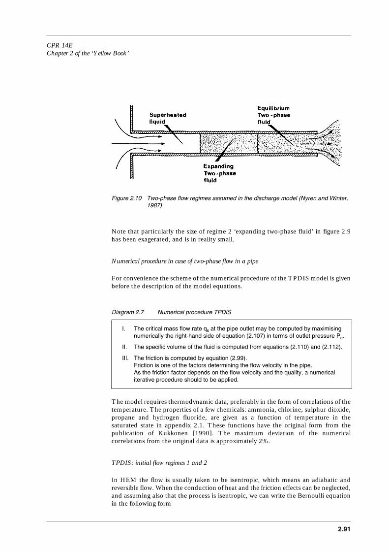
CPR 14EChapter 2 of the ‘Yellow Book’
2.91
Figure 2.10 Two-phase flow regimes assumed in the discharge model (Nyren and Winter, 1987)
Note that particularly the size of regime 2 ‘expanding two-phase fluid’ in figure 2.9has been exagerated, and is in reality small.
Numerical procedure in case of two-phase flow in a pipe
For convenience the scheme of the numerical procedure of the TPDIS model is givenbefore the description of the model equations.
Diagram 2.7 Numerical procedure TPDIS
The model requires thermodynamic data, preferably in the form of correlations of thetemperature. The properties of a few chemicals: ammonia, chlorine, sulphur dioxide,propane and hydrogen fluoride, are given as a function of temperature in thesaturated state in appendix 2.1. These functions have the original form from thepublication of Kukkonen [1990]. The maximum deviation of the numericalcorrelations from the original data is approximately 2%.
TPDIS: initial flow regimes 1 and 2
In HEM the flow is usually taken to be isentropic, which means an adiabatic andreversible flow. When the conduction of heat and the friction effects can be neglected,and assuming also that the process is isentropic, we can write the Bernoulli equationin the following form
I. The critical mass flow rate qs at the pipe outlet may be computed by maximising numerically the right-hand side of equation (2.107) in terms of outlet pressure Pe.
II. The specific volume of the fluid is computed from equations (2.110) and (2.112).
III. The friction is computed by equation (2.99).Friction is one of the factors determining the flow velocity in the pipe.As the friction factor depends on the flow velocity and the quality, a numerical iterative procedure should to be applied.
2.92
u2/2 = Cd2 × (∫ vF × dP + g × hf) (m2/s2) (2.93)
where
u = fluid flow velocity [m/s]Cd = discharge coefficient [-]vF = specific volume of the fluid [m3/kg]P = pressure [N/m2]g = gravitational acceleration [m/s2]hf = fluid height [m]
The discharge coefficient (Cd) is a measure for pressure loss of the liquid flow at thepipe inlet (not related to the outflow at the pipe exit). The pipe is assumed to have auniform bore. The ratio qS/Ap is called the mass flux G defined by
G = qS/Ap = u/vF (kg/(m2⋅s)) (2.94)
where
qS = mass flow rate (discharge rate) [kg/s]Ap = cross-sectional area of the pipe [m2]
For very short pipes, smaller than 0.1 m, the discharge of pressurised liquefied gasescan be assumed to remain in liquid form. For liquid flow, the fluid is incompressibleand the equation (2.93) reduces in flow regimes 1 and 2 to the form of
qS = Cd × Ap/vL × √(2(vL × (P0-P2)+g × ∆hL,2)) (kg/s) (2.95)
where
vL = specific volume of the liquid phase [m3/kg]P0 = initial pressure in the vessel [N/m2]P2 = pressure at the end of flow regime 2 [N/m2]∆hL,2 = liquid height difference in the flow regime 2 [m]
The vertical coordinate axis is chosen to be in the upward direction, and
∆hL,2 = hL,0 - hL,2 (m) (2.96)
where
hL,0 = liquid height pipe inlet [m]hL,2 = liquid height pipe at end of flow regime 2 [m]
Equation (2.95) gives the mass flow rate at the end of the flow regime 2. Thisequation can also be applied in estimating liquid discharges through breaches incontainer wall or through very short pipes.
CPR 14EChapter 2 of the ‘Yellow Book’
2.93
TPDIS: mass flux equation
In the third regime, the conservation of the total energy of the fluid gives
vF × dP + d(u2/2) + u2 × fD/(2 × dp) × dx + g × dhL = 0 (m2/s2) (2.97)
where
dp = inner pipe diameter [m]fD = friction factor [-]x = length variable along the pipe [m]vF = specific volume of the fluid [m3/kg]
The first term in equation (2.97) is the energy per unit mass due to change of state ofthe fluid. The second term is the kinetic energy, and the third term is the energy lossdue to flow friction at pipe walls and the fourth term is the potential energy.The third term in equation (2.97) can be derived from the theory of the turbulentboundary layer flows, applied to pipes by Landau and Lifschitz. It has been assumedthat the laminar friction forces are in general much smaller than the forces governingthe turbulent energy dissipation.The friction factor is a function of the roughness of the pipe divided by the pipediameter ε/dp, and the Reynolds number Re. The friction factor for turbulent flow in smooth and rough pipes can be computedfrom the Colebrook-White law for the transition zone
1/√fD = -2 × 10log(2.51/(Re × √fD) + ε/(3.715 × dp)) (-) (2.98)
Equation (2.98) is an implicit equation for fD. Chen has shown that the followingexplicit equation gives the same numerical results with an accuracy greater than 0.5%
(-) (2.99)
with
C1 = 3.7065C2 = 2.5226C3 = 1.1098C4 = 2.8257C5 = 5.8506C6 = 0.8981
This equation is valid for 4000 < Re <107. (2.100)
The Reynolds number is given by
Re = u × dp × ρtp/ηtp (-) (2.101)
1 fD⁄ 2.0ε
dp----- 1
C1------
2 C2×
Re--------------ε
dp-----
C3 1C4------
C5
ReC6-----------+×
log10
×–×
log10
×–=
2.94
where
u = fluid flow velocity [m/s]dp = pipe diameter [m]ρtp = density two-phase fluid [kg/m3]ηtp = dynamic viscosity two-phase fluid [N⋅s/m2]
The dynamic viscosity is given by
ηtp = ηL × (1-Φm × (1-(ηL/ηV))) (-) (2.102)
where
ηL = dynamic viscosity of liquid phase [N⋅s/m2]ηV = dynamic viscosity of vapour phase [N⋅s/m2]Φm = quality or mass fraction of vapour [-]
in two-phase mixture
Φm,e can be found by equation (2.112).
In integrating equation (2.97) over the third regime, unsolvable integrals of thespecific volume and the density appear. These integrals can be estimated as follows.We define the volume and density ratio parameters CAr and CBr
∫ vF × dx = CAr × vF,e × lp (m4/kg) (2.103)
- ∫ ρF⋅dhL = CBr × ρL × ∆hL,3 (kg/m2) (2.104)
with
∆hL,3 = hL,2-hL,e (m) (2.105)
where
vF,e = specific volume fluid at the outlet [m3/kg]ρF = density fluid [kg/m3]ρL = liquid density [kg/m3]lp = pipe length [m]hL,2 = height pipe at end of flow regime 2 [m]hL,e = height pipe outlet [m]∆hL,3 = height difference in third regime [m]
The volume and density ratio parameters are measures of the rate of evaporation inthe equilibrium flow regime. As the fluid is initially liquid and the specific volume ofthe fluid increases in the equilibrium flow regime, the following limits are obtained
if lp -> 0 then CAr and CBr -> 1.0 (2.106a)
if lp -> ∞ then CAr and CBr -> 0.5 (2.106b)

CPR 14EChapter 2 of the ‘Yellow Book’
2.95
The lower limits of CAr and CBr are only approximative; possible values for CAr andCBr are between these limits.If there is phase equilibrium in the tank and the pipe is relatively short, let us saywithin a few metres, the change in the specific volume of the fluid is relatively small.Numerical estimates show that the volume ratio parameter is in the range0.7<CAr<0.9. If there is phase equilibrium in the tank and the pipe is relatively long,0.5<CAr<0.7. If there is overpressure in the tank relative to the saturation vapourpressure, CAr≈1.0. These values apply approximately also for the density ratioparameter CBr. The ratio parameters CAr and CBr are computed in the model fromnumerical correlations, based on the values mentioned above.
The following correlations are suggested:
if 0 <= lp <= 3 CAr = CBr = 1 – 0.1 x lp (2.106c)
if 3 < lp <= 20 CAr = CBr = 0.7 – (lp – 3) x 0.2 / 17 (2.106d)
if lp > 20 CAr = CBr = 0.5 (2.106e)
Thus CAr and CBr decrease linearly from 1 to 0.7 over the first three meters pipelength (2.106c) and have a constant value of 0.5 above 20 meters (2.106e). Along theintermediate region the parameters decrease linearly from 0.7 to 0.5 (2.106d).
The values of the volume ratio parameter CAr are not known precisely in the model.However, it was found that the numerical results are not sensitive to variations in thisparameter; it can be shown that inaccuracies in estimating CAr cause only a few percent error in the mass flux values. The same result also applies to variations in thedensity ratio parameter CBr.
Equation (2.97) can now be integrated over regime 3, using the definitions (2.103)and (2.104). Finally, combination with equation (2.95) yields the following equationfor the mass flux density qS/Ap at the outlet
(kg2/(m4⋅s2)) (2.107)
with
τi = vF,i/vF,e (-) (2.108)
where
Ki = resistance coefficient [-]Pe = pressure at the pipe exit [N/m2]vvi = specific volume at resistance site pipe [m3/kg]vve = specific volume at the exit [m3/kg]τi = specific volume ratio [-]
qS Pe( )
Ap----------------- 2 P0 Pe–( )
gVL------- hL ,2 CBr hL ,3∆×+∆( )×+
vF ,e Pe( ) 1× lp fD CAr 2 dp×( )⁄××( ) Σ Ki τi 2⁄×( ) vL Pe( ) Cd⁄ 1 1 2 Cd×( )⁄–( )×–+ +[ ]---------------------------------------------------------------------------------------------------------------------------------------------------------------------------------------------------------------------------------=
2.96
The critical mass flow rate qs at the pipe outlet may be computed by numericallymaximising the right-hand side of equation (2.107) in terms of the outlet pressure Pe.
The values of the resistance coefficients are determined by the geometrical structureof the pipe system. In subsection 2.5.5 resistance coefficients have been given.
The gravity term increases the mass flux for a downward flow (hL>0, h2>0) anddecreases it for an upward flow. The parameter CBr describes the reduced effect ofgravity on two-phase flow, due to fluid vaporisation. The effective density of the fluidin regime 3 is given by CBr/vL
The influence of gravity on two-phase pipe flow depends on the height differenceduring flow, on the physical properties of the chemical and on the pressure in thecontainer. Clearly, gravity is more important for small container pressures. Forinstance, for chlorine releases at 15 ˚C, assuming pipe lengths of 1-5 m and pipeinclination angles from 10˚ to 20˚, the effect of gravity on the mass flux isapproximately 10%.
TPDIS: specific volume and the quality
The discharge rate can be solved from equation (2.107) using the critical flowcondition if the specific volume of the two-phase fluid as a function of pressure ve(Pe)is known. The mass flow rate is critical when
(dqS/dPe)c = 0 (m⋅s) (2.109)
The critical exit pressure is less than the reservoir stagnation pressure and higher thanthe ambient pressure at pipe exit.The specific volume of the two-phase fluid at the exit aperture can be written in termsof the vapour and liquid phase specific volumes by
vF,e(Pe) = Φm,e(Pe) × vVs(Pe) + (1-Φm,e(Pe)) × vLs(Pe) (m3/kg) (2.110)
where
Φm,e = vapour mass fraction (quality) at pipe outlet [-]vF,e = specific fluid volume at pipe outlet [m3/kg]vVs(Pe)= specific saturated vapour volume at pipe outlet [m3/kg]vLs(Pe)= specific saturated liquid volume at pipe outlet [m3/kg]
The compressibility of the vapour and liquid phases has also been taken into account,as the saturation state properties have been used.The mass fraction of vapour phase at the pipe outlet can be computed using theisentropic assumption
SL(T0,P0) = Φm,e(Pe) × SVs(Pe) + (1-Φm,e(Pe)) × SLs(Pe) (J/(kg⋅K)) (2.111)

CPR 14EChapter 2 of the ‘Yellow Book’
2.97
where
SL(T0,P0) = specific entropy liquid phase at initial conditions [J/(kg⋅K)]SLs(Pe) = specific entropy saturated liquid phase at pipe outlet [J/(kg⋅K)]SVs(Pe) = specific entropy saturated vapour phase at pipe outlet [J/(kg⋅K)]
In appendix 2.2 of this section entropy and enthalpy have been given for a fewcompounds as a function of temperature.
It can be shown that this yields
Φm,e(Pe) = Te,s(Pe)/Lv,e(Pe) × (SLs(P0)-SLs(Pe)) (-) (2.112)
where
Lv,e = heat of evaporation of the liquid at pipe outlet [J/kg]Te,s(Pe) = saturated fluid temperature at pipe outlet [K]
at exit pressure
The saturated fluid temperature at pipe outlet at given exit pressure Tes(Pe) can befound through the saturation curve. By the assumption of thermodynamicequilibrium the saturation pressure equals the exit pressure
P˚v(Te,s) = Pe (N/m2) (2.113)
It must be stated that the TPDIS model predicts rather high exit pressures.
The influence of the pipe geometry and the fluid properties on the mass flux
Figure 2.11 shows the influence of pipe length and pipe diameter on the mass flowrate. The ambient temperature has been set at 15 ˚C.
Figure 2.11 The mass flow rate versus pipe length in a chlorine discharge, for various pipe diameters [Kukkonen, 1990]
2.98
The decrease in mass flux with pipe length is mainly due to flow friction. The effectof flow friction depends on the relative roughness of the pipe wall (ε/dp), and on theReynolds number. The influence of flow friction on the mass flux is typically less than10% for short pipes (lp<2 m); however, its influence may be much greater forpipelines. Changing the roughness of the pipe wall in the range from 0.01 millimetreto 0.1 millimetre (the assumed value was 0.05 millimetre) causes a change ofapproximately 10% in the mass flow rate.
2.5.3.6 Non-stationary two-phase propane flow in pipelines
The modelling of the two-phase flow through pipelines aims at predictingthe mass flow rate as a function of time depending on the initial conditions.
Transient release from full bore ruptured pipelines
The model given by Morrow [1983] has been derived for propane, but could begeneralised by using appropriate physical properties. The model has been designed for initial pipeline pressures at the location of the breakthat are (much) higher than the saturation pressure [Dodge, 1996].The model estimates the mass flow rate from one side of the ruptured pipeline.This model is used for the entire region of two-phase flow within the pipeline. At thepoint of pipe rupture, the upstream and downstream end of the pipe are assumed tobe totally separated so that the flow rates coming from the upstream and downstreampipe regions are independent. Both flows are determined initially on the basis ofchoked flow at the pipe exit. As time progresses, the flow rate diminishes untilchoking (equivalent to sonic flow in a perfect gas discharge) no longer occurs.The model of Fauske is used to determine the correlation of pressure just inside thepipe exit and flow rate during choked flow. An analysis of two-phase flow pressuregradient and void fraction (vapour volume) has been developed to provide the massdepletion in the pipe as a function of exit flow rate and pressure. These correlationsfor exit flow and pipe flow together allow correlations for exit flow versus time afterrupture.
The basic assumptions are briefly as follows. The Fauske equation for critical flow atthe exit Gcr of a full pipe break is used.Away from the point of rupture, the frictional pressure drop of the pipeline is givenby the Fanning equation, which has been explained in subsection 2.5.5.The slip ratio used, i.e. the ratio of vapour velocity to liquid velocity, can be calculatedusing the relation of Fauske
uV/uL = √(ρL/ρV) (-) (2.114)
The thermodynamic properties HL,0, HL, Lv and vL are relatively insensitive tochanges in pressure. This makes it possible, though not necessary, to correlate someterms of the equations with a simple (intermediate) polynomial function Fi(P). Bydoing this, computation time can be saved. For propane the coefficients of thesecorrelations are given.
CPR 14EChapter 2 of the ‘Yellow Book’
2.99
Intermezzo
The Fauske equation for critical flow at the exit Gcr of a full pipe break is given byequation (2.115).Together with the subsequent equations up to and including equation (2.121) thecritical flow can be estimated as a function of the unknown exit pressure Pe.
1/Gcr2 = - dΦm/dP ×
-2vL + 2√(vL × vV) - 4Φm × √(vL × vV) + 2Φm × vL + 2Φm × vV
- dvV/dP × Φm × √(vL/vV) -Φm2 × √(vL/vV) +Φm
2 (2.115)
with
Φm = (HL,0-HL)/Lv (-) (2.116)
The derative of quality Φm with respect to pressure is found from the derative of liquidenthalpy, latent heat and vapour specific volume, by
dΦm/dP = - 1/Lv × dHL/dP + Φm × (dLv/dP) + 0.5 × Φm × uL2/vL × (dvV/dP)
(m2/N) (2.117)
The thermodynamic properties HL,0, HL, Lv and vL are relatively insensitive tochanges in pressure, so that
dΦm/dP ≈ - 0.5/Lv × Φm × uL2/vL × (dvV/dP) (m2/N) (2.117a)
A method for expressing uL as a function of pressure makes use of the slip ratio usedby Fauske. The following equation can be inferred:
F1(P) = (qS × vL/(A × uL))2
(-) (2.118)
The value of the bracketed term is influenced primarily by vV(P), the otherthermodynamic quantities are relatively insensitive to changes in pressure.Note that the right-hand term of equation (2.118) is dimensionless.
Coefficients Ci can be calculated by the polynomial approximation of theintermediate function F1(P) which includes only thermodynamic quantities:
F1(P) ≈ CC1 + CC2 × P + CC3 × P2 + CC4 × P3 (-) (2.118a)
For propane:
CC1 = -0.0081 [-] (2.118b)CC2 = 3.1785 × 10⁻⁷ [(m2/N)]CC3 = 1.8820 × 10⁻¹³ [(m2/N)2]CC4 = 9.4027 × 10⁻¹⁹ [(m2/N)3]
m4s2
kg2-----------
= Lv/ HL ,0 HL–( )( ) vL/vV( )×
1 Lv/ HL ,0 HL–( ) 1–( ) vL/vV( )×+------------------------------------------------------------------------------------
2
2.100
Equation (2.117) and (2.117a) contain a factor (dvV/dP).The non-stationary flow in a pipeline of a pressurized liquefied gas may be consideredas an adiabatic process. This means that we are looking for a function f(P,T) whichsatisfies the following equation
(dv/dP)s = f(P,T) (m4⋅s2/kg2) (2.119)
Combining equations (2.9c) and (2.39a) shows the relationship between thedifferential and the speed of sound in the vapour phase
(dv/dP)s = -1/(ρV × us,V)2 (m4⋅s2/kg2) (2.120)
By equation (2.39c) the speed of sound in the vapour phase can be estimated.However, being stored as a pressurized liquefied gas the approximation by perfect gasbehaviour may not be accurate. The introduction of the compressibility factor z fornon-ideal gases shifts the problem towards finding an expression for z=z(P,T).In the original publication Morrow [1983] referred to Starling [1983] who presentedan equation of state for several chemicals, like butane, carbon dioxide, ethane, ethene,hydrogen sulphide, methane, and propane. Data for other chemicals, like for instanceammonia, can be found in [Edminster, 1984].
The unknown exit pressure Pe can be estimated if a boundary condition for the massflow rate at the exit qs,e is given, which could be a function of the exit pressure Pe too.Then it is possible to calculate the exit pressure Pe corresponding to qs,e by arootfinding numerical routine, solving the following equation
Gcr - qS,e/Ap = 0 (2.121)
Note that exit pressure Pe will be somewhere between the ambient pressure Pa andthe saturation pressure Pv˚(T0).
Where
Ap = pipe cross-sectional area [m2]Gcr = critical mass flux at the exit [kg/(m2⋅s)]HL = specific enthalpy of saturated liquid [J/kg]HL,0 = specific enthalpy of saturated [J/kg]
liquid at initial storage temperatureLv = latent heat of vaporisation [J/kg]P = pressure [N/m2]Pa = ambient pressure [N/m2]Pe = exit pressure [N/m2]Pv˚(T)= saturation pressure [N/m2]qs = mass flow rate [kg/s]qs,e = mass flow rate at the exit [kg/s]uV = vapour velocity [m/s]uL = liquid velocity [m/s]us,V = speed of sound in vapour [m/s]T0 = initial temperature [K]Φm = quality [-]ρL = liquid density [kg/m3]ρV = vapour density [kg/m3]vL = specific volume saturated liquid [m3/kg]vV = specific volume vapour [m3/kg]
CPR 14EChapter 2 of the ‘Yellow Book’
2.101
Numerical procedure in case of two-phase propane flow from complete ruptured pipelines
1. When the initial pressure P0 in the pipeline is much higher than the saturationpressure, the initial discharge flow rate (t = 0) at the pipe break location can beestimated by assuming sonic liquid outflow through the end of the pipe [Dodge,1996]
qS,e,1 = Ap × (P0-Pe)/us,L (kg/s) (2.122)
whereP0 = initial pressure in the pipeline [N/m2]us,L = speed of sound in liquid [m/s]
The initial estimate of mass flow is based on an acoustic decompression of thecompressed liquid in the pipeline at the break location.
The speed of sound in chemicals that are commonly stored as a pressure liquefied gas,like propane, ammonia and chlorine, is not easily found in literature as is its pressuredependency.The speed of sound in the liquid phase of a few chemicals stored as a pressureliquefied gas at a temperature of 288.15 K [NIST] are presented in the table:
Most liquids have a speed of sound between 900 m/s and 1500 m/s, and on theaverage about 1250 m/s. Liquid propane and propene are both one of the exceptions.An increase of pressure will increase the speed of sound. In most cases a pressureincrease of about 100 bars will increase the speed of sound in liquids about 5-15%.So, when the initial mass flow rate calculated by equation (2.121) is based on thesound speed at moderate pressures conditions, the estimate will be somewhatconservative.
Use the scheme presented in the intermezzo above, equations (2.115-2.121), toestimate the unknown exit pressure, and the initial discharge flow rate qs,e,l implicitly.
In case of propane outflow a better estimate for the initial mass flow rate for moderatepressures could be calculated by Tam’s model, equation (2.137). For other chemicalsat moderate pressures the correction factor (2.137b) could be applied.
2. Assume a lower value for the exit mass flow rate
qS,e,2 = 0.95 × qS,e,1 (kg/s) (2.123)
chemical Pv˚(T)(105 ⋅ N/m2)
us,L(m/s)
propane 7.31 786.2propene 8.91 715.1ammonia 7.27 1361butane 1.82 950.6

2.102
3. Calculate the average flow rate at the exit
= 0.5⋅(qS,e,1+qS,e,2) (kg/s) (2.124)
4. Calculate the new exit pressure Pe corresponding to qS,e,2, by the schemepresented in the intermezzo, equations (2.115-2.121), using the followingboundary condition
Gcr = qS,e,2/Ap (kg/(m2⋅s)) (2.125)
5. Calculate the distance to the interface ∆li, from
∆li = (m) (2.126)
with intermediate correlation F2
F2(P) = C1 × P + C2/2 × P2 + C3/3 × P3 + C4/4 × P4 (N/m2) (2.127)
The upstream flow rate at interface where two-phase flow starts qS,us is set to be zeroafter the pumps are shut down.
Note that the intermediate function F2 is the integral of intermediate function F1given by equation (2.118a).
Where
dp = inner pipe diameter [m]fF = Fanning friction factor [-]uL = velocity liquid phase [m/s]∆li = distance from rupture to interface [m]
6. Neglecting the vapour density in comparison with liquid density, the massremoved from the pipeline Qyi,2 can be calculated by equation
Qyi,2 = (kg) (2.128)
with
F4(P) = CB1 × P + CB2/2 × P2 + CB3/3 × P3 + CB4/4 × P4 + CB5/5 × P5
(N/m2) (2.128a)
Qyi = quantity of mass removed from pipeline by void formation
Note that initially Qyi,1 = 0.
qS eav,
3 dp Ap2 F2 Pi( ) F2 Pe( )–[ ]×××
2 fF vL qS ,e2
2×××------------------------------------------------------------------------
3 dp Ap3 F4 Pi( ) F4 Pe( )–[ ]×××
2 fF vL2 qS ,e
2×××------------------------------------------------------------------------

CPR 14EChapter 2 of the ‘Yellow Book’
2.103
The coefficients CBi can be calculated by the polynomial approximation of theintermediate function F3(P) which includes only thermodynamic quantities.
F3(P) = Φv × F1
= F1 / [ 1 + (Lv/(HL,0-HL)-1) × √(vL/vV) ] (-) (2.129)
F3(P) ≈ CB1 + CB2 × P + CB3 × P2 + CB4 × P3 + CB5 × P4 (-) (2.129a)
The intermediate function F4 is the integral of intermediate function F3.Note that the right-hand term of equation (2.129) is dimensionless.The value of the bracketed term is influenced primarily by vV(P).
For propane:
CB1 = -5.5695 × 10⁻³ [-] (2.128b)CB2 = 2.94896 × 10⁻⁷ [(m2/N)]CB3 = -1.27218 × 10⁻¹³ [(m2/N)2]CB4 = 1.34158 × 10⁻¹⁸ [(m2/N)3]CB5 = -1.8414 × 10⁻²⁴ [(m2/N)4]
7. Calculate the time increment in step i for mass removed
∆ti = (Qyi,2 - Qyi,1)/qS,e,av (s) (2.130)
8. The exit mass flow rate at the beginning of the next time step qs,e,l must be setequal to the exit mass flow rate at the end of the previous time step qs,e,2.
Repeat the numerical procedure for each new time-step by starting again with step2, until the distance to the interface ∆li is larger than the pipelength Lp or if time tis smaller than the specified time for which the outflow rate or the conditions inthe pipeline must be estimated.
Note that the time after the rupture is given by
t = Σ∆ti (s) (2.130a)
By comparing the initial mass content in the pipeline with the mass removed Qyi,2 itmay appear that the pipeline is not empty after the last time step. If so, it isrecommended to continue the predicted mass flow rate of the last time step until allremaining mass will be removed. The duration of this stage of the release is given by
∆tE = (ρ0 × Ap × Lp - Qyi,2) / qs,e,2 (s) (2.130b)
where
∆tE = duration release remaining liquid [s]ρ0 = initial liquid density [kg/m3]

2.104
Remark
If the pipeline has been ruptured in the middle (‘double’ guillotine break), then theoverall mass flow rate from the pipeline is twice the calculated value by this model.
In case the rupture is near one of the pipe ends or an isolation valve, both parts of theoriginal pipeline should be regarded as two independent sources.
The way Morrow accounted for pumping rate in the pipeline apparent before thebreak, is not correct.Dodge [1996] has given several useful comments on Morrow’s model, amongstothers on how to cope with a pumping rate in the pipeline.In case of a ‘double’ guillotine break to the first order the pumping rate does notinfluence the venting rate, and to account for the pumping rate to consider secondorder effects would make the computational model much more complicated. In caseof a guillotine break the fluid vents from both the upstream and downstream sides ofthe guillotine break.On the upstream side, the pumping rate (which is in the same direction as the ventingflow) adds to the initial estimate of the venting rate, and thus it will increase all thesubsequent computations of upstream venting rate from Fauske’s model. On thedownstream side, the pumping rate (which is in the opposite direction as the ventingflow) subtracts from the initial estimate of the venting rate, and thus it will decreaseall the subsequent computations of downstream venting rate from Fauske’s model.The net effect is that the pumping rate tends to cancel out of the venting ratecalculations (but not quite) when the upstream and downstream venting rates areadded together.For this reason the pumping rate for the ‘double’ guillotine break case can beneglected, certainly at the early stages of the release.
Transient release from leaking or (partially) ruptured propane pipelines
A simple exponential correlation has been fitted against experiments with 100 metrepropane pipeline of 0.150 m diameter and 0.05 m diameter orifice plate [Tam, 1990].A characteristic of the transient releases in the test data was found to be that the totalmass of propane inside the test line decreases exponentially with time after a periodof flow establishment. The flow establishment lasted from less than 1 to about5 seconds, depending on the size of the test orifice. The release rate does not decayexponentially in this period. In the experiments the duration of the established flowwas 20 seconds or more, again depending on the orifice size.
The model for the transient releases rate is given by
d Q(t)/dt = -Cα × Q(t) (kg/s) (2.131)
where
Cα = constant of decay [1/s]Q = mass content pipeline [kg]t = time from the start of the release [s]
CPR 14EChapter 2 of the ‘Yellow Book’
2.105
While by definition the mass flow rate from the pipe is given by
qS(t) = - d Q(t)/dt (kg/s) (2.132)
the following equation can be inferred from the model as formulated by Tam [1990]
qS(t) = Cα × Q0 × e-Cα⋅t (kg/s) (2.133)
qS = mass flow rate [kg/s]
The main factors which affect the value of the exponential decay constant wereassessed using statistical analysis. These factors were the initial fluid conditions, suchas fluid temperature, and the test line configurations, such as pipe length and orificearea. The following regression was obtained from the data set
Cα = dR0.25 × (0.22 × AR - 0.13 × + CCα × (T0-288.15))
(1/s) (2.134)
with
dR = dp[m] / 0.05 [m] (-) (2.134a)
AR = Ah/Ap (-) (2.134b)
and
CCα = 0.00068 [K-1] (2.134c)
WhereAh = cross-sectional area hole [m2]Ap = cross-sectional area pipe [m2]AR = area ratio [-]dp = pipe diameter [m]dR = radius ratio [-]T0 = initial (absolute) temperature fluid [K]
The deviation between the predictions and the measured results is less than 20%.The experiments did not result in any significant correlation between the initialpressure and the value of the decay constant.
Range of experimental parameters:
Although the variation in length of the pipeline has been recognised by Tam as afactor governing the exponential decay of the transient release rate, no correlationbetween the mass flow rate and the pipe length was given.
Initial pressure P0 [N/m2] 7.5⋅105 - 22⋅105
Initial temperature T0 [K] 287.15 - 297.15Pipe diameter dp [m] 0.05 - 0.15Area ratio AR [m2/m2] 0.04 - 1.0
AR1.5
2.106
Note that equations (2.131) and (2.132) imply that the initial mass flow rate seemsto depend on the initial mass content of the pipe, and thus on the length of thepipeline, since
q0 = q(t=0)
= Cα × Q(t=0) (kg/s) (2.135)
with
Q0 = Q(t=0)
= ρL(T0) × Vp
= ρL,0 × π/4 × dp2 × Lp (kg) (2.136)
where
Q0 = initial mass content pipeline [kg]Lp = length pipeline [m]Vp = pipeline volume [m3]ρL,0 = density propane at initial temperature T0 [kg/m3]
This can not be true, which means that the model can not be used for pipe lengthsother than 100 m.However, the model can give a good impression of the magnitude of the initial flowrate after the flow establishment region by
q0 = Cα × CLp × ρL,0 × π/4 × dp2 (kg/s) (2.137)
with somewhat artificially
CLp = 100 m (2.137a)
It must be mentioned however, that the duration of the flow establishment will be afunction of the length of the pipeline.
In an engineering approach we could define a (general) correction factor CTam by
CTam = q0,Tam/q0,L (-) (2.137b)
with
q0,Tam = propane mass flow rate estimated by equation (2.137)q0,L = propane mass flow rate estimated by equation (2.199)
This correction factor can be used to improve the estimation of the initial mass flowrate for any pressure liquefied gas assuming pure liquid outflow.The latter two quantities should be calculated for the same conditions.

CPR 14EChapter 2 of the ‘Yellow Book’
2.107
2.5.3.7 Finite duration spray releases
This section provides the models to describe the behaviour of the two-phasejets into the atmosphere from pressurised liquefied gases. First, the effects associatedwith the depressurisation of the release to atmospheric pressure are described.Secondly, the possibility of rain-out of droplets to the ground (forming an evaporatingpool) is addressed. Therefore, the droplet size is estimated and the evaporation of adroplet falling through the air. Finally the effects of the evaporation of the dropletsremaining in the air are described, leading to an effective density and concentrationof the vapour/air mixture that will disperse in the atmosphere. The methodologies arepresented stepwise in Diagram 2.8.
Diagram 2.8 Stepwise overview of models to describe two-phase jets
In this section extensive use is made of thermodynamical properties of chemicals.Knowledge is required of the following material properties: density of liquid andvapour as a function of temperature and pressure, enthalpy as a function oftemperature, kinematic viscosity of the liquid phase, latent heat, surface tension of theliquid-vapour interface, molar weight, saturation pressure as a function oftemperature and the binary diffusion coefficient of the vapour in air. For a number ofchemicals these data are collected in the Annex of this Yellow Book. In some casese.g. (the binary diffusion coefficient) approximate values are presented in the text.
Step 1 - Calculate the conditions in the jet after flashing
The outflow conditions can be characterised by the following quantities:– the pressure at the exit Pe [N/m2],– the temperature at the exit Te (K),– the effective cross-section of the exit opening Ae [m
2],– the total mass flow rate qS,e [kg/s], which is the product of exit cross-section Ae
[m2] and mass flux [kg/(m2⋅s)], and– the vapour mass fraction (or ‘quality’) at the exit Φm,e (kg vapour per kg two-phase
mixture).
Step 1 Calculate the conditions in the jet after flashing in the atmosphere is complete: – flash fraction– jet velocity– radius and density of flashed jet
Step 2 Calculation of the droplet diameter after flashing
Step 3 Droplet evaporation and rain-out on the ground:First determine if droplets may reach the ground;If so, calculate the liquid mass fraction that will reach the ground.
Step 4 Calculate the conditions in the jet after evaporation of all airborne droplets: – concentration– jet velocity– radius and density of the single-phase jet

2.108
In case of outflow through a hole in a vessel wall the exit conditions are identical tothe (bulk) conditions in the vessel.In case of outflow from piping or pipeline the exit conditions refer to the conditionsin the pipe before the outflow opening.
The density at the exit ρe [kg/m3] can be calculated from the vapour density ρV,e at Peand Te, the liquid density ρL,e at Te and the quality Φm,e:
(m3/kg) (2.138)
After the exit the flow will depressurise to atmospheric pressure and liquid will flashto vapour until the two-phase mixture is at boiling temperature. From conservationof momentum and conservation of mass the jet velocity after flashing can becalculated:
(m/s) (2.139)
Here Pa is the ambient pressure, and ue is the velocity in the exit which follows fromthe exit density ρe and the mass flux. From the conservation of total energy the qualityafter flashing can be calculated:
(-) (2.140)
Here, HV,e and HV,f are the vapour enthalpies [J/kg] for the exit temperature andboiling temperature, respectively. Lv,e and Lv,f are the latent heat of evaporation atexit conditions and after flashing, respectively. The average jet density after flashingρf is calculated using (2.138) by changing in this formula lower index e by lower indexf. Now the increase of the jet cross-section Af and jet radius bf can be calculated fromconservation of mass:
(m2; m) (2.141)
Step 2 - Calculation of the droplet diameter after flashing
In order to estimate the possibility of rain-out (droplets from the jet falling to theground and not contributing directly to the amount of pollutant in the jet), it isnecessary to calculate the droplet diameter after flashing. In reality, all droplets have different diameters. Here, we only calculate a singledroplet diameter which will be assumed to be representative of all droplets.The droplet diameter depends on jet velocity, jet size, viscosity and surface tension.Therefore, use is made of two dimensionless numbers, the Reynolds number Ref andthe Weber number Wef. The Reynolds number characterises the balance betweenmomentum and kinematic viscosity ν, the Weber number characterises the balancebetween momentum and surface tension σs:
1ρe-----
1 Φm e,–( )
ρL e,------------------------
Φm e,
ρV e,-----------+=
ufPe Pa–( )Ae
qs e,--------------------------- ue+=
Φm f, 1HV f, HV e,– 1 Φm e,–( )Lv e,
12--
uf2 ue
2–( )+ +
Lv f,------------------------------------------------------------------------------------------------–=
Af
ρeue
ρfuf----------Ae bf
Af
π-----==

CPR 14EChapter 2 of the ‘Yellow Book’
2.109
(-;-) (2.142)
Here, bf is the jet radius and uf is the jet velocity after flashing, ρL,f is the density andνL is the kinematic viscosity of the liquid after flashing, and σs is the surface tensionbetween the liquid and the vapour.
The droplet size can now be estimated by the following correlations:
– If Wef < Ref-0.45 × 10⁶ and Te < 1.11TB (where TB is the normal boiling
temperature), then:
(m) (2.143a)
– Else:
(m) (2.143b)
Here ρa is the density of air (ambient gas).In the literature values for the constant Cds vary between 10 and 20. Here a value of15 is recommended. Large droplets falling to the ground will break-up according to the second of theabove correlations, inserting the free fall velocity ud for uf. This requires an iterativesolution using the above correlation and formula (2.145) for ud in the followingsection.
Step 3 - Droplet evaporation and rain-out on the ground
In this section, first an estimate is made whether droplets originating from the flashingcan fall to the ground. If this is the case, the total mass fraction that will fall on theground is calculated.The droplets are assumed to have the same diameter: the evolution of the singledroplet diameter due to evaporation is therefore assumed to be representative of alldroplets.Estimation of droplet rain-out requires calculation of the rate of evaporation ofindividual droplets. The evaporation is restricted by a heat flux from the ambient airto the droplet and by the mass flux from the droplet surface into the ambient air.Therefore, the problem depends on convection and diffusion of heat and mass in air.The relevant dimensionless numbers are the Reynolds number Red, based on therelative velocity of the droplet through the air, the Schmidt number Sc, the ratio ofviscosity to mass diffusion, and the Prandtl number Pr, the ratio between viscosityand heat diffusion. These numbers will be used in the following calculations. Thelatter two numbers only depend on the properties of air and the released chemical:
(-;-;-) (2.144a,b,c)
Ref
2bfuf
υL------------ Wef
2bfuf 2ρL f,
σs-----------------------==
dd 3.78bf 1 3Wef
1
2--
Ref----------+
=
dd Cds
σs
uf 2 ρa
-------------=
Reduddd
υa----------- Sc
υa
D----- Pr
Cpρaυa
λ-----------------===
2.110
In these definitions, ud is the relative velocity of the droplet in surrounding air. In thefollowing formulae, it is assumed that ud equals the free fall velocity of the droplet. νais the kinematic viscosity of the ambient air, dd is the droplet diameter. D is the binarydiffusion coefficient of the vapour through air. Cp is the specific heat, ρa the densityand λ is the conductivity of heat of the ambient air. For the Prandtl number in air atabout 288 K one can use Pr=0.71. If no data on the binary diffusion constant D areavailable, one can also assume Sc≈0.7.
The velocity ud is assumed to be the final free fall velocity. For small droplets, use canbe made of Stokes’ flow regime which is strictly valid for Red < 1, but the results arenot sensitive to this assumption:
(m/s) (2.145)
Here ρL,f is the density of the droplet at boiling temperature (i.e. the condition afterflashing), and g is the acceleration of gravity (g≈9.8ms-2).For the calculation of the evaporation from the droplet, first a coefficient kB is definedwhich governs the evaporation at the droplets’ surface:
(m2/s) (2.146)
Here, µi is the molar weight of the released chemicals, Pa is the ambient pressure, Rthe universal gas constant (R = 8.31434 J × mol-1K-1), Ta is the ambient temperature,and Pv˚(Td) is the saturation pressure of the released chemical at the droplettemperature.
Now, first the temperature difference between the ambient air and the droplet needsto be calculated. This so-called temperature depression maintains the required heatflux from the air to the droplet in order to enable the evaporation. This requires theiterative solution of the following equation. The solution needs to be iterative as thesaturation pressure Pv˚ as included in the evaluation of kB, is strongly dependent onthe droplet temperature Td. It is not necessary to evaluate the droplet density ρL andthe Reynolds number Red for each iteration:
(K) (2.147)
It is now possible to approximate the maximum diameter of a droplet that will rain-out from a release height hs above the ground:
(m) (2.148)
ud
ρL f, g
18υaρa----------------dd
2=
kB
4µiDPa
ρL f, RTa------------------- 1
Ps Td( )
Pa----------------–
ln=
Td Ta
Lv d, kBρL f, 1 0.28Red
1
2--Sc
1
3--
+
4λ 1 0.28Red
1
2--Pr
1
3--
+
---------------------------------------------------------------------–=
dM 2 9ρaυakBhs
2ρL f, g------------------------ 1 0.204Sc
1
3-- ρL f, g
18ρaυa2----------------
1
2--
72ρaυakBhs
ρL f, g-----------------------------–
3
8--
1–1
4--
=
CPR 14EChapter 2 of the ‘Yellow Book’
2.111
This approximation is applicable if Red (based on dM) < 4. Rain-out will only occurif the droplet size after flashing dd is larger than the maximum rain-out droplet dM.If dd is smaller than dM, and Red (based on dM) < 4, one may skip to the next section.
If dd is larger than dM or Red > 4, the total mass that will rain-out and the mass thatremains in the air need to be calculated. Therefore, a numerical integration needs tobe performed of the evolution of the diameter of the droplet as it evaporates whilefalling down. The evolution of the droplet diameter dd(t) can be calculated from thedifferential equation:
(m/s) (2.149)
Here Red depends on the droplet diameter according to (2.144) and (2.145). Theheight above the ground of the droplet is calculated by integrating the velocity ud,which also varies with time according to (2.145), over time. It is assumed that therelease is horizontal, and that there is no initial vertical velocity component. Theintegration is performed until the droplet hits the ground, i.e. h(t0)=0. Therefore, t0follows implicitly from the following expression:
(m) (2.150)
In practice, as ud depends on the droplet size, (2.149) and (2.150) are simultaneouslynumerically integrated until z=0. By comparing the droplet size d0 when the droplet hits the ground to the initialdroplet size after flashing, dd, the evaporated mass fraction while falling to the ground,can be calculated. This in turn will lead to the nett mass released to the air by the jet:
(kg/s) (2.151)
Here, qS,e is the mass flow rate through the release opening, and Φm,f the vapour massratio or quality after flashing. The first term refers to the vapour initially in the jetwhile the second term refers to the vapour released while the droplets fall to theground. The latter process leads to a cooling of the air entrained in the vapour/aerosolcloud. This cooling process will be described in the following section, but it requiresthe redefinition for the quality and the jet cross-section after flashing in case rain-outoccurs, i.e.:
(-) (2.152)
(m2; m) (2.153)
In case rain-out occurs, in the following sections Φm,f, Af, and qS,e should be replacedby Φm,f, rainout, Af, rainout, and qS,nett,air.
ddt-----dd
kB
dd----- 1 0.28Red
1
2--Sc
1
3--
+–=
0 h t0( ) hs u d td0
t0
∫–==
qs nett ,air, Φm f, qs e, 1 Φm f,–( ) 1d0
dd-----
3
– qs e,+=
Φm f rainout, ,
Φm f,
Φm f, 1 Φm f,–( ) 1d0
dd-----
3
– +
------------------------------------------------------------------=
Af rainout, Af
qs nett ,air,
qs e,--------------------- bf rainout,
Af rainout,
π---------------------==

2.112
Step 4 - Calculate the conditions in the jet after evaporation of all airbornedroplets
The evolution of a two-phase jets in terms of air entrainment, width, concentrationdecay and velocity decay is the same as the evolution of single-phase jets as describedin chapter 4.In order to perform subsequent dispersion modelling using dispersion models whichdo not account for two-phase effects in the plume or cloud, this section provides thetechnique to calculate the cooling of the single-phase jet after all airborne dropletshave evaporated. More details about coupling are provided in section 2.7.2.2.The concentration in the jet corresponding to the amount of air which has to beentrained into the jet in order to evaporate all aerosols, has to be calculated in aniterative way from the enthalpy balance. The total changes in enthalpy due totemperature change, evaporation of aerosol or condensation of ambient humidity,need to be zero:
(J/mol) (2.154)
The terms in the foregoing enthalpy balance will be evaluated separately below. The molar fraction cj of the vapour in the jet is equal to the partial vapour pressure.As long as droplets are present up to the moment when all liquid has just evaporated,the partial vapour pressure equals the saturation pressure at the jet temperature Tj:
(-) (2.155)
If all liquid aerosol has evaporated, the quality or vapour mass fraction Φm,j is zero.In that case the enthalpy change of the released chemical since flashing follows from:
(J/mol) (2.156)
Here, µs is the molar mass of the released chemical, Lv,f is the latent heat ofevaporation, and Hf and Hj the specific enthalpies at boiling temperature and jettemperature, respectively.The enthalpy changes of air depend on the humidity of the air. The mass fraction ofwater vapour in the ambient dry air (it is assumed no water droplets or mist arepresent in the ambient air) is given by:
(-) (2.157)
Here, RHa is the ambient relative humidity, Ps,w(Ta) is the saturation pressure ofwater at ambient temperature Ta, R is the gas constant, µw is the molar weight ofwater, and ρa is the density of ambient air.
∆ Hchemical( ) ∆ Hdry air( ) ∆ Hwater vapour( ) 0=+ +
cjPv
o Tj( )
Pa---------------=
∆ Hchemical( ) cjµs 1 Φm f,–( )Lv f,– Hf Hj–+[ ]=
mw
mda---------
RHaPv w,o Ta( )
R/µw( )Taρa--------------------------------=
CPR 14EChapter 2 of the ‘Yellow Book’
2.113
After the air in the jet has cooled down to jet temperature Tj, part of the water vapourmay condense. The remaining mass fraction of vapour is calculated by:
(-) (2.158)
The molar fraction of water vapour to dry air at ambient temperature and jettemperature, respectively, are:
(-) (2.159)
Here µa and µw are the molar weights of (dry) air and water, respectively (µa =28.96⋅10-3 kg/mol, µw = 18.02⋅10-3 kg/mol.The enthalpy change of entrained dry air can now be calculated by:
(J/mol) (2.160)
Here Cp is the specific heat of air.The enthalpy change of the water entrained with the air is:
(J/mol) (2.161)
Here, Lw,j is the latent heat of water at jet temperature, and Cp,w is the specific heatof water vapour.The jet temperature and molar fraction or volume concentration cj can be calculatediteratively from the expressions above. First, an initial temperature Tj is chosen forwhich the molar fraction cj can be calculated using (2.155). Then the contributionsT to the enthalpy balance can be evaluated and the total sum can be calculated from(2.154). By means of an iterative procedure (Regula Falsi) new values of Tj can beselected in order to minimise the sum of enthalpy changes.The situation in the jet just after complete evaporation of the liquid aerosols ofreleased material (note water aerosols are likely to be present), is relevant in order tocalculate the total (negative) buoyancy released to the air. The density of the jet canbe calculated as follows. First, the equivalent molar mass of the vapour mixtures iscalculated:
(kg/mol) 2.162)
The density of the vapour only follows from the perfect gas law:
(kg/m3) (2.163)
In order to account for the condensed water vapour, the additional water liquid molarfraction is calculated:
(-) (2.164)
mwv
mda---------
TaPv w,o Tj( )
RHaTjPv w,o Ta( )
--------------------------------------=
cw
mwµa
mdaµw--------------- cwv
mwvµa
mdaµw---------------==
∆ Hdry air,( )1 cj–( )
1 cwv+( )-------------------- Cpµa= Ta Tj–( )
∆ Hwater vapour( )1 cj–( )
1 cwv+( )--------------------µw Cp w, Ta Tj–( )[ ]=
µjd cjµs
1 cj–( )
1 cwv+( )-------------------- µa cwvµw+( )+=
ρjdPaµjd
R Tj------------=
cjL
1 cj–( )
1 cwv+( )-------------------- cw cwv–( )
µw
ujd------=
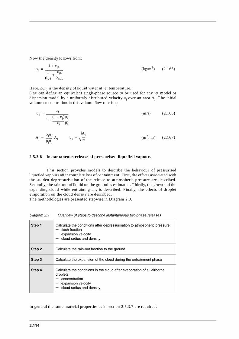
2.114
Now the density follows from:
(kg/m3) (2.165)
Here, ρw,L is the density of liquid water at jet temperature.One can define an equivalent single-phase source to be used for any jet model ordispersion model by a uniformly distributed velocity uj over an area Aj. The initialvolume concentration in this volume flow rate is cj:
(m/s) (2.166)
(m2; m) (2.167)
2.5.3.8 Instantaneous release of pressurised liquefied vapours
This section provides models to describe the behaviour of pressurisedliquefied vapours after complete loss of containment. First, the effects associated withthe sudden depressurisation of the release to atmospheric pressure are described.Secondly, the rain-out of liquid on the ground is estimated. Thirdly, the growth of theexpanding cloud while entraining air, is described. Finally, the effects of dropletevaporation on the cloud density are described. The methodologies are presented stepwise in Diagram 2.9.
Diagram 2.9 Overview of steps to describe instantaneous two-phase releases
In general the same material properties as in section 2.5.3.7 are required.
Step 1 Calculate the conditions after depressurisation to atmospheric pressure: – flash fraction– expansion velocity– cloud radius and density
Step 2 Calculate the rain-out fraction to the ground
Step 3 Calculate the expansion of the cloud during the entrainment phase
Step 4 Calculate the conditions in the cloud after evaporation of all airborne droplets:– concentration– expansion velocity– cloud radius and density
ρj1 cjL+
1ρj d,--------
cjL
ρw L,----------+
-------------------------=
ujuf
11 cj–( )
cj----------------+
µa
µs-----
------------------------------=
Aj
ρfuf
ρjuj--------- Af bj
Aj
π-----= =

CPR 14EChapter 2 of the ‘Yellow Book’
2.115
Step 1 - Calculate the conditions in the cloud after depressurisation
The storage conditions as they prevail in the containment prior to the release will beassumed to be input for the calculations.
These conditions are:
Storage temperature T0 (K)Pressure P0 (N/m)Total mass stored Q (kg)Vapour mass fraction Φm,0 (-) (to be derived from the fill level of the vessel)
The expansion to atmospheric pressure leads to flashing and evaporation of liquid.After flashing, the temperature TB equals the normal boiling temperature of thereleased chemical.The vapour mass fraction Φm,f after flashing can be calculated assuming isentropicflashing:
(-) (2.168)
Here Lv,0 and Lv,f are the latent heat of the chemical at storage and boilingtemperature, respectively, and S0,L and Sf,L are the entropy of the liquid chemical atstorage temperature and pressure and boiling temperature and ambient pressure,respectively. If no detailed data on entropies are available, this can be approximatedby:
(-) (2.169)
Here Cp,L is the specific heat of the liquid.It is assumed that the stored chemical is initially at rest. During flashing theliquid/vapour cloud will expand with a velocity which follows from the conservationof total energy during flashing. This energy balance also includes the work performedon the ambient air. The real expansion velocity will be about 20% lower than thevalue which follows directly from the energy balance because part of the kineticenergy will be transferred to turbulence and the flashing process will probably not beisentropic. So the expansion velocity uf is approximated by:
(m/s) (2.170)
Here H0,V and Hf,V are the vapour enthalpy of the released chemical at storagetemperature and boiling temperature, respectively. ρ0 is the average density of the
Φm f,
Φm 0,
Lv 0,
T0--------- S0 L, Sf L,–+
Lv f,
Tf--------
----------------------------------------------------=
Φm f, Φm 0, Tf
T0------
Tf
Lv f,--------+ Cp L,
T0
Tf------ln=
uf 0.8 2 H0 V, Hf V, 1 Φm f,–( )Lv f, 1 Φm 0,–( )Lv 0,
P0 Pa–
ρ0----------------––+–
=
2.116
chemical in the vessel, which can be calculated by (2.138), thereby changing index eto index 0.
The total volume Vf after flashing follows from
(m3) (2.171)
Here ρf is calculated by (2.138) thereby changing index e to index f. For a vessel onthe ground the expanding cloud will be a hemisphere. After flashing the radius of thehemisphere will be:
(m) (2.172)
Step 2 - Calculate the rain-out fraction to the ground
The amount of liquid raining out from the cloud depends on the flash fraction. If Φm,f< 0.5, twice the initial flash fraction will remain airborne, i.e.:
(kg) (2.173)
If Φm,f > 0.5, no rain-out is assumed. If rain-out occurs, the vapour mass fraction inthe cloud needs to be redefined. From the calculation of Qnett,air it follows that in thatcase always Φm,f,rainout=0.5. It is also necessary to redefine the cloud density ρf(formula 2.138 using Φm,f,rainout), Vf and bf. In the following sections one shouldreplace Q, Φm,f ρf, Vf and bf by these redefined values if rain-out occurs.The fraction of total mass not remaining in the air will form an evaporating pool onthe ground.
Step 3 - Calculate the expansion of the cloud during the entrainment phase
It is assumed that after flashing air is entrained in the cloud. The concentration of airand released chemical in the cloud are uniform throughout the cloud.If we define tf to be the time when flashing is complete, i.e. when the radius b equalsbf, the evolution with time after flashing of the radius and expansion velocity of thecloud can be calculated by:
(m) (2.174)
(m/s) (2.175)
VfQρf----=
bf
3Vf
2π--------
1 3/
=
Qnett ,air 2Φm f, Q=
b t( ) 4ufbf 3 t tf–( ) bf
4+[ ]
1
4--
=
u t( ) uf bf
b t( )---------
3
=

CPR 14EChapter 2 of the ‘Yellow Book’
2.117
Step 4 - Calculate the conditions in the cloud after evaporation of allairborne droplets
In order to calculate the extent of the two-phase cloud and to enable coupling withdispersion models which need an initial cloud size, this section provides the methodto determine the size of the cloud when all aerosol has evaporated and the expansionvelocity is reduced to the wind velocity at the cloud height after flashing bf.The determination of the amount of entrained air needed to evaporate all liquidaerosol (except condensed water from the water vapour contained in the air), or, inother words, the required concentration cj, is performed as described in section2.5.3.7, (2.154) to (2.165), reading ‘cloud’ for ‘jet’. These formulae also provide theaveraged cloud density ρj.The cloud volume Vj and radius bj at the moment all aerosol has evaporated areapproximately:
(m3; m) (2.176)
Here ρs,j is the density of the vapour of pure released chemical (i.e. it is not thecloud averaged density) at the cloud temperature Tj. The initial volumeconcentration in this cloud is cj. Subsequent dispersion modelling can now take place if the expansion velocity uj islower than the wind speed ua at the cloud height after flashing bf. uj can be calculatedusing (2.175) if bj is inserted for b(t).
If uj > ua(bf), the radius of the cloud bdisp and the volume Vdisp (input for dispersionmodelling) can be calculated from:
(m; m3) (2.177)
Assuming that the averaged molar specific heat of the cloud after evaporation is equalto the molar specific heat of air, the temperature Tdisp of the cloud of volume Vdispcan be calculated by:
(K) (2.178)
The molar or volume concentration cdisp at this stage of the cloud is:
(-) (2.179)
The cloud density ρdisp can be estimated (neglecting the effect of water vapour ordroplets) by formulae (2.162) and (2.163) (section 2.5.3.7), assuming cwv = 0 andinserting Tdisp and cdisp for Tj and cj, respectively.The initial clouds Vj or Vdisp (depending on whether the cloud expansion velocity ujexceeds the windspeed) can be used as initial conditions for dispersion models.
VjQ
cjρs j,----------- bj
3 Vj
2π---------
1
3--
==
bdisp bf uf
ua bf( )--------------
1
3--
Vdisp2
3--πb
3disp==
TdispTa
1Vj
Vdisp----------- 1 Ta
Tj------–
–----------------------------------------=
cdisp cjVj
Tdisp
VdispTj------------------=

2.118
2.5.4 Liquids
2.5.4.1 Vessel dynamics liquid
The modelling of the dynamics of a vessel filled with (non-boiling) liquidaims at predicting the decrease of liquid mass during the outflow of liquid.
The hydraulic pressure driving the mass flow rate depends on the liquid level in thetank; a constant pressure P by compression with inert gas may be taken into account.
Applying the basic law of conservation of mass, and taking into account the hydraulicpressure of a liquid column, will suffice for an adequate description of the vesseldynamics.
The model is basically an iterative numerical procedure in which the outflow of liquidout of a vessel is described in small steps. These steps should be small enough toconsider the conditions in the vessel to be constant during one time-step.
First, the initial condition and termination condition of the numerical procedure willbe given. Next, the model in the form of a numerical procedure is given. Thisnumerical procedure has to be repeated until the termination conditions have beensatisfied.Finally, equations relating the liquid height to the liquid volume in the vessel for fewvessel shapes are given.
Initial conditions and termination procedure (non-boiling) liquid outflow from a vessel
The initial condition of the vessel (i=1) is given by its filling degree φ, constanttemperature and vessel volume.The liquid mass in the vessel can easily be calculated given the (initial) filling degreeφ, by
QL,1 = φ × V × ρL(T) (kg) (2.180)
where
QL,1 = liquid mass initially in the vessel [kg]φ = filling degree [m3/m3]V = vessel volume [m3]ρL = liquid density at storage temperature [kg/m3]
The initial liquid volume can be estimated by
VL,1 = QL,1/ρL (m3) (2.181)
CPR 14EChapter 2 of the ‘Yellow Book’
2.119
The initial liquid height can be estimated by using the inverse function between liquidvolume and liquid height for the given geometry of the vessel (see next sub-paragraph:eq. (2.193a), (2.193b), (2.193c), expressed by
hL,1 = F-1(VL,1) (m) (2.182)
The duration of δt may be chosen freely in principle, and depends of the number oftime-steps Nt. The choice Nt=50 will be appropriate for most calculations. If onewishes to estimate the mass flow rate and vessel conditions at time tend, then the sizeof time-step δt is given by
δt = tend/Nt (s) (2.12)
The numerical procedures given should be repeated as long as the constraints arevalid
ti < tend hL > hhole (2.183)
The larger the number of steps, the higher the accuracy of the model, but the moretime needed for the calculation. The choice N=50 will be appropriate, for mostcalculations.
Numerical procedure non-boiling liquid outflow from a vessel
Starting every step at time ti in the iteration with a condition in the vessel given byQL,i the following procedure aims at calculation of the condition in the vessel at theend of the small time-step δt, given by QL,i+1.
Let us say that the outflow rate qS,i is given by a generalised function f, depending onwhether the outflow is through a hole or a pipe (see paragraph 2.5.4.2)
qS,i = f(hL,i,P,...) (kg/s) (2.184)
The conservation of mass leads very simply to
δQ = - qS,i × δt (kg) (2.185)
The liquid content will decrease with
δVL = δQ/ρL (m3) (2.186)
thus
VL,i+1 = VL,i + δVL (m3) (2.187)
For simple geometries equations are available to calculate the liquid volume and thesize of the liquid area as a function of the liquid level.In general the following formulation holds

2.120
AL,i = f(hL,i,...) (m2) (2.188)
Then the new liquid level can be calculated by
δhL = δVL/AL,i (m) (2.189)
hL,i+1 = hL,i + δhL (m) (2.190)
The time from the start of the release must be increased by one time-step after everypass through this numerical procedure
ti+1 = ti + δt (s) (2.191)
The new condition of the vessel at time ti+1 is given by: QL,i+1 or hL,i+1.This numerical procedure has to be repeated until the termination conditions havebeen satisfied.
Liquid height as a function of liquid volume
For simple geometries equations are available to calculate the liquid volume VL andthe size of the liquid surface in the vessel AL as a function of the liquid level hL, in thegeneralised form expressed by
AL = F(hL) (m2) (2.192)
VL = F(hL) (m3) (2.193)
For instance, the following relations hold for a few geometries
* sphere
AL = π × (r2-(r-hL)2) (m2) (2.192a)
VL = π/3 × h2Lf × (3 × r-hL) (m3) (2.193a)
* horizontal cylinder
AL = 2 × L × √((2 × r-hL) × hL) (m2) (2.192b)
VL = L × [r2 × acos(1-hL/r) - (r-hL) × √((2 × r-hL) × hL] (m3) (2.193b)
* vertical vessel
AL = Abase (m2) (2.192c)
VL = AL × hL (m3) (2.193c)
CPR 14EChapter 2 of the ‘Yellow Book’
2.121
Where
AL = liquid surface inside vessel [m2]Abase = base vertical cylinder [m2]hL = liquid height [m]VL = liquid volume in vessel [m3]r = radius of the sphere or cylinder [m]
2.5.4.2 Liquid outflow through holes and piping
The modelling of the outflow of liquid through holes and piping aims atpredicting the mass flow rate as a function of the pressure drop.
Liquid flow through holes or orifices
For liquids flowing through an orifice the Bernoulli equation can be applied.Neglecting the initial liquid velocity in the vessel, the mass flow rate can be estimatedby
(kg/s) (2.194)
with
P = Ph + PaL (N/m2) (2.195)
and
Ph = ρL × g × hL (N/m2) (2.196)
Ah = cross-sectional area of the hole [m2]Cd = discharge coefficient [-]g = gravitational acceleration [m/s2]hL = (relative) liquid height [m]P = total pressure at opening [N/m2]Ph = (hydraulic) liquid pressure [N/m2]PaL = external pressure above liquid [N/m2]Pa = atmospheric pressure [N/m2]qS = mass flow rate [kg/s] ρL = liquid density [kg/m3]
The following values for the discharge coefficients are recommended; Beek [1975].
For sharp orifices
Cd = 0.62 (-) (2.197a)
for straight orifices
Cd = 0.82 (-) (2.197b)
qs Cd Ah 2 P Pa–( ) ρL×( )××=
2.122
for rounded orifices
Cd = 0.96 (-) (2.197c)
and for a pipe rupture
Cd = 1.0 (-) (2.197d)
Liquid flow through pipes
The pressure drop for a stationary fluid flow in piping can be estimated by the well-known Darcy-Weisbach equation.
∆P = fD × ρf/2 × uf2 × lp/dp (N/m2) (2.198)
Using this equation, an expression for the (average) liquid flow velocity in the pipecan be inferred
(m/s) (2.199)
The mass flow rate in the pipe can be calculated by
qS = ρ × uL × Apipe (kg/s) (2.200)
where
dp = pipe diameter [m]fD = Darcy friction factor [-]lp = pipe length [m]uL = liquid flow velocity [m/s]∆P = pressure over the pipe [N/m2]ρL = liquid density [kg/m3]
According to the equations above, the mass flow rate through a pipe depends on thefriction in the pipe.In general the friction factor is a function of the Reynolds number (see paragraph2.5.5).The Reynolds number, depending on the flow velocity in the pipe, can be expressedas a function of the mass flow rate
Re = f(qS) (2.201)
For circular pipes
Re = (4/π) × qS/(dp × η) (-) (2.201a)
This means that the mass flow rate in the pipe has to be calculated by iteration.
uL 2 P lp dp fD ρL×( )⁄×⁄∆×( )=
CPR 14EChapter 2 of the ‘Yellow Book’
2.123
2.5.5 Friction factors
Fluid flows in pipes and pipe fittings are associated with friction. Thefriction causes a pressure drop depending on the roughness of the pipe wall and onthe shape of the pipe fitting.
Friction in straight pipes
The Colebrook-White law yields the friction factor as a function of pipe diameter,roughness of the inner pipe wall, flow velocity and viscosity.If used in combination with the Darcy-Weisbach equation, the two equations areconsidered by many authorities as the best equations available for determining thehead loss for turbulent flow in commercial pipes, as stated by Ackers in 1963[Radford,1990].
The Darcy friction factor fD can be predicted by the Colebrook-White law for thetransition zone
1/√fD = -2 × 10log(ε/(3.715 × dp) + 2.51/(Re × √fD)) (-) (2.202)
The Reynold’s number characterises the flow of fluids and is given by
Re = ρ × u × dp/η (-) (2.101)
Equation (2.201) can be solved by applying a root finding procedure, and defining anauxiliary function
F(fD) = 1/√fD + 2 × 10log(ε/(3.715 × dp) + 2.51/(Re × √fD)) (-) (2.202a)
The auxiliary function F(fD) equals zero for that fD which is the solution of equation(2.201), where
fD = Darcy friction factor [-]dp = pipe diameter [m]ε = wall roughness [m]Re = Reynolds number [-]uf = fluid flow velocity [m/s]ρf = fluid density [kg/m3]η = dynamic viscosity [N⋅s/m2]
The Darcy-Weisbach equation also predicts the head loss in the pipe
∆hLp = fD × lp × uf2/(2 × g × dp) (m) (2.198a)
Where
g = gravitational acceleration [m/s2]∆hLp = head loss [m]lp = pipe length [m]
2.124
The head loss ∆hLp and pressure drop are simply related
∆P = ρf × g × ∆hLp (N/m2) (2.203)
As apparent from equation (2.202) the Darcy factor is a function of the Reynoldsnumber and the relative wall roughness (the ratio between the wall roughness and thepipe diameter). For the wall roughness the values in the table below can be used.
Table 2.2 Some values for wall roughness for pipes
The pressure drop for a stationary fluid flow in piping is also often estimated by theDarcy Weisbach equation in which the Fanning friction factor is used
∆P = 4 × fF × ρf/2 × uf2 × lp/dp (N/m2) (2.204)
where
fF = Fanning friction factor for flow in pipes [-]
From the equations, (2.198) and (2.204) it easy to conclude that the Fanning frictionfactor is four times smaller than the Darcy friction factor
4 × fF = fD (m) (2.205)
When applying the equations from literature one should check which factor is referredto.
For the Darcy friction other equations and graphics are well-known.For laminar flow
fD = 64/Re if Re < 2000 (-) (2.206)
For turbulent flow and smooth pipe the Blasius equation holds
fD = 0.3164 × Re-0.25 if 4000 < Re < 105 (-) (2.207)
Friction is one of the factors determining the flow velocity in the pipe. As the frictionfactor depends on the Reynolds number being a function of velocity, in general aniterative procedure should to be applied to estimate the mass flow rate in the pipe.However, according to figure 2.12 ‘Friction factor for flow in pipes’ it appears thatthe friction factor is virtually constant for sufficiently high Reynolds numbers.
Material Wall roughness ε
Bronze, lead, glass 1.5 µmCommercial steel, wrought-iron 45 µmCast iron 250 µm
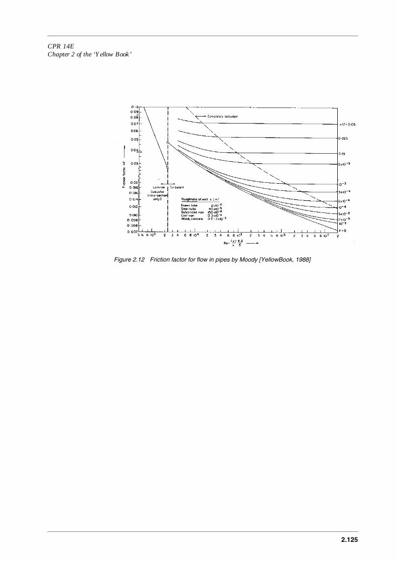
CPR 14EChapter 2 of the ‘Yellow Book’
2.125
Figure 2.12 Friction factor for flow in pipes by Moody [YellowBook, 1988]
2.126
Non-circular pipes
For non-circular pipes the so-called hydraulic diameter may be used which is definedas
dh = 4 × Ap/sp (m) (2.208)
where
Ap = cross-sectional area the pipe [m2]sp = wetted perimeter of the pipe [m]
Note that for circular tubes the hydraulic diameter is equal to the pipe diameter.
The use of Hazen-Williams and Manning relations should be discouraged, butempirical equations are quoted in text books and many people working in the field ofhydraulic engineering still prefer them [Radford, 1990]. Additional information can be found in for instance Melhem [1993] and Radford,[1990].
Frictional pressure drop in pipe fittings
The models for outflow through pipes are developed for a pipe with no bends,reductions of cross-section or branches. If such elements are present, they can beaccounted for by introducing an extra resistance coefficient.
The relation between the pressure drop and the kinetic energy per element of volumeof the transported product is called the friction or resistance coefficient
Ki = ∆P/(1/2 × ρf × u2) (-) (2.209)
where
Ki = resistance coefficient [-] ∆P = pressure drop due to friction [N/m2]ρf = density of the fluid [kg/m3]u = flow velocity of the fluid [m/s]
For pipe elements the resistance coefficient Ki has the following values
45˚-bend : 0.35 90˚-bend : 0.75 open spherical valve : 6.4 half-open spherical valve : 9.5 inlet piece with sharp edges : 0.5
CPR 14EChapter 2 of the ‘Yellow Book’
2.127
2.6 Application of the selected models: calculation examples
2.6.1 Introduction to section 2.6
The models presented in this chapter can be divided into iterative modelsand non-iterative models.Non-iterative models facilitate predictions by applying a set of equations once. Forthis type of model calculation examples have been worked out step by step.
Iterative models facilitate predictions only by repeating a (complex) numericalprocedure a (great) number of times. A step-by-step approach would not be practical.For this type of model the final results will be given only as a function of specifiedinput.
2.6.2 Compressed gases
2.6.2.1 Hydrogen outflow from a vessel through a hole in the vessel wall
The hydrogen outflow from of a vessel through a hole in the vessel wall canbe calculated by the models presented in paragraphs 2.5.2.2 and 2.5.2.3.
Input:
Initial pressure P0 = 50 barInitial temperature T0 = 288.15 KVessel volume V = 100 m3
Leak size dh = 0.1 m(cross-sectional area hole Ah = 7.854⋅10-3 m2)Discharge coefficient Cd = 0.62 -Time from start release t = 30 sThermodynamic model Adiabatic
Output:
Mass flow at 30 sec qS = 4.65 kg/sGas pressure at 30 sec P = 12.417 barGas temperature at 30 sec T = 193 K
Procedure
The number of time-steps Nt has been set to equal 50.By equation (2.22) the mass flow rate qs,i at the beginning of every time-step can becalculated. Because the pressure in the vessel is much larger than about 1.9⋅Pa, thegas flow is critical initially.

2.128
Using the equations (2.14) and (2.20) subsequently and assuming perfect gasbehaviour (z=1), the variation of the vessel conditions (Pi, Ti, ρi) due to the outflowcan be calculated.
In table 2.3 the variations in the physical quantities have been given.
Table 2.3
Time after rupture Flowrate Hole pressure Gas temperature Total mass release
[s] [kg/s] [bar] [°C] [kg]
0.00 15.31 50.000 15.00 0,00
0.60 14.92 48.494 12.47 9.07
1.20 14.53 47.037 9.97 17.90
1.35 14.44 46.681 9.35 20.07
1.50 14.34 46.328 8.74 22.23
1.80 14.16 45.630 7.51 26.51
2.10 13.98 44.945 6.29 30.73
2.40 13.80 44.271 5.08 34.89
2.70 13.62 43.609 3.87 39.00
3.00 13.45 42.959 2.67 43.06
3.30 13.27 42.319 1.48 47.07
3.60 13.10 41.690 0.30 51.03
3.90 12.94 41.072 -0.87 54.93
4.20 12.77 40.464 -2.04 58.79
4.50 12.61 39.867 -3.20 62.60
4.80 12.45 39.280 -4.35 66.36
5.10 12.30 38.702 -5.49 70.07
5.40 12.14 38.135 -6.63 73.74
5.70 11.99 37.576 -7.76 77.36
6.00 11.84 37.027 -8.88 80.93
6.30 11.69 36.488 -10.00 84.46
6.60 11.55 35.957 -11.11 87.95
6.90 11.40 35.435 -12.21 91.39
7.20 11.26 34.922 -13.30 94.79
7.50 11.12 34.417 -14.39 98.14
7.80 10.98 33.920 -15.47 101.46
8.10 10.85 33.432 -16.55 104.73
8.40 10.72 32.952 -17.61 107.97
8.70 10.58 32.479 -18.67 111.16
9.00 10.45 32.015 -19.73 114.32
9.30 10.33 31.558 -20.78 117.43
9.60 10.20 31.108 -21.82 120.51
9.90 10.08 30.666 -22.85 123.55
10.20 9.95 30.230 -23.88 126.56
10.50 9.83 29.802 -24.90 129.53
10.80 9.71 29.381 -25.92 132.46
11.10 9.60 28.967 -26.93 135.35
11.40 9.48 28.559 -27.93 138.22
11.70 9.37 28.158 -28.93 141.04
12.00 9.25 27.763 -29.92 143.83
12.30 9.14 27.375 -30.90 146.59
12.60 9.03 26.993 -31.88 149.32
12.90 8.92 26.617 -32.86 152.01
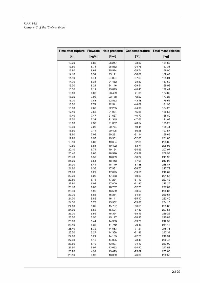
CPR 14EChapter 2 of the ‘Yellow Book’
2.129
13.20 8.82 26.247 -33.82 154.68
13.50 8.71 25.882 -34.78 157.31
13.80 8.61 25.524 -35.74 159.90
14.10 8.51 25.171 -36.69 162.47
14.40 8.41 24.824 -37.63 165.01
14.70 8.31 24.482 -38.57 167.52
15.00 8.21 24.146 -39.51 169.99
15.30 8.11 23.815 -40.43 172.44
15.60 8.02 23.489 -41.35 174.86
15.90 7.93 23.168 -42.27 177.25
16.20 7.83 22.852 -43.18 179.62
16.50 7.74 22.541 -44.09 181.95
16.80 7.65 22.235 -44.99 184.26
17.10 7.56 21.934 -45.88 186.55
17.40 7.47 21.637 -46.77 188.80
17.70 7.39 21.345 -47.66 191.03
18.00 7.30 21.057 -48.54 193.23
18.30 7.22 20.774 -49.41 195.41
18.60 7.14 20.495 -50.28 197.57
18.90 7.05 20.221 -51.14 199.69
19.20 6.97 19.951 -52.00 201.80
19.50 6.89 19.684 -52.86 203.88
19.80 6.81 19.422 -53.71 205.93
20.10 6.74 19.164 -54.55 207.97
20.40 6.66 18.910 -55.39 209.98
20.70 6.59 18.659 -56.22 211.96
21.00 6.51 18.413 -57.05 213.93
21.30 6.44 18.170 -57.88 215.87
21.60 6.36 17.931 -58.70 217.79
21.90 6.29 17.695 -59.51 219.69
22.20 6.22 17.463 -60.33 221.57
22.50 6.15 17.234 -61.13 223.42
22.80 6.08 17.009 -61.93 225.26
23.10 6.02 16.787 -62.73 227.07
23.40 5.95 16.569 -63.52 228.87
23.70 5.88 16.354 -64.31 230.64
24.00 5.82 16.141 -65.10 232.40
24.30 5.75 15.932 -65.88 234.13
24.60 5.69 15.727 -66.65 235.85
24.90 5.63 15.524 -67.42 237.54
25.20 5.56 15.324 -68.19 239.22
25.50 5.50 15.127 -68.95 240.88
25.80 5.44 14.933 -69.71 242.52
26.10 5.38 14.742 -70.46 244.15
26.40 5.32 14.553 -71.21 245.75
26.70 5.27 14.368 -71.96 247.34
27.00 5.21 14.185 -72.70 248.91
27.30 5.15 14.005 -73.43 250.47
27.60 5.10 13.827 -74.17 252.00
27.90 5.04 13.652 -74.90 253.52
28.20 4.99 13.479 -75.62 255.03
28.50 4.93 13.309 -76.34 256.52
Time after rupture Flowrate Hole pressure Gas temperature Total mass release
[s] [kg/s] [bar] [°C] [kg]

2.130
2.6.2.2 Carbon monoxide flow through hole in a pipe
The carbon monoxide outflow from a vessel through a pipe can becalculated by the model presented in paragraph 2.5.2.4.
Input:
Vessel volume V = 100 m3
Constant pressure upstream P0 = 15 barInitial temperature T0 = 288.15 KPipe length lp = 1000 mPipe diameter dp = 0.254 mInternal wall roughness pipe ε = 4.5⋅10-5 mLeak size dh = 0.1 m(cross-sectional area hole Ah = 7.854⋅10-3 m2)Discharge coefficient Cd = 0.62 -
Output:
Mass flow at t = 0 s qS = 15.615 kg/s
Procedure
The four steps of the numerical procedure given in paragraph 2.5.2.4. have to berepeated several times. By using equation (2.30a) the number of iterations can belimited by a root finding procedure.
28.80 4.88 13.142 -77.06 257.99
29.10 4.83 12.977 -77.77 259.44
29.40 4.77 12.814 -78.48 260.88
29.70 4.72 12.653 -79.19 262.31
30.00 4.67 12.495 -79.89 263.72
Time after rupture Flowrate Hole pressure Gas temperature Total mass release
[s] [kg/s] [bar] [°C] [kg]
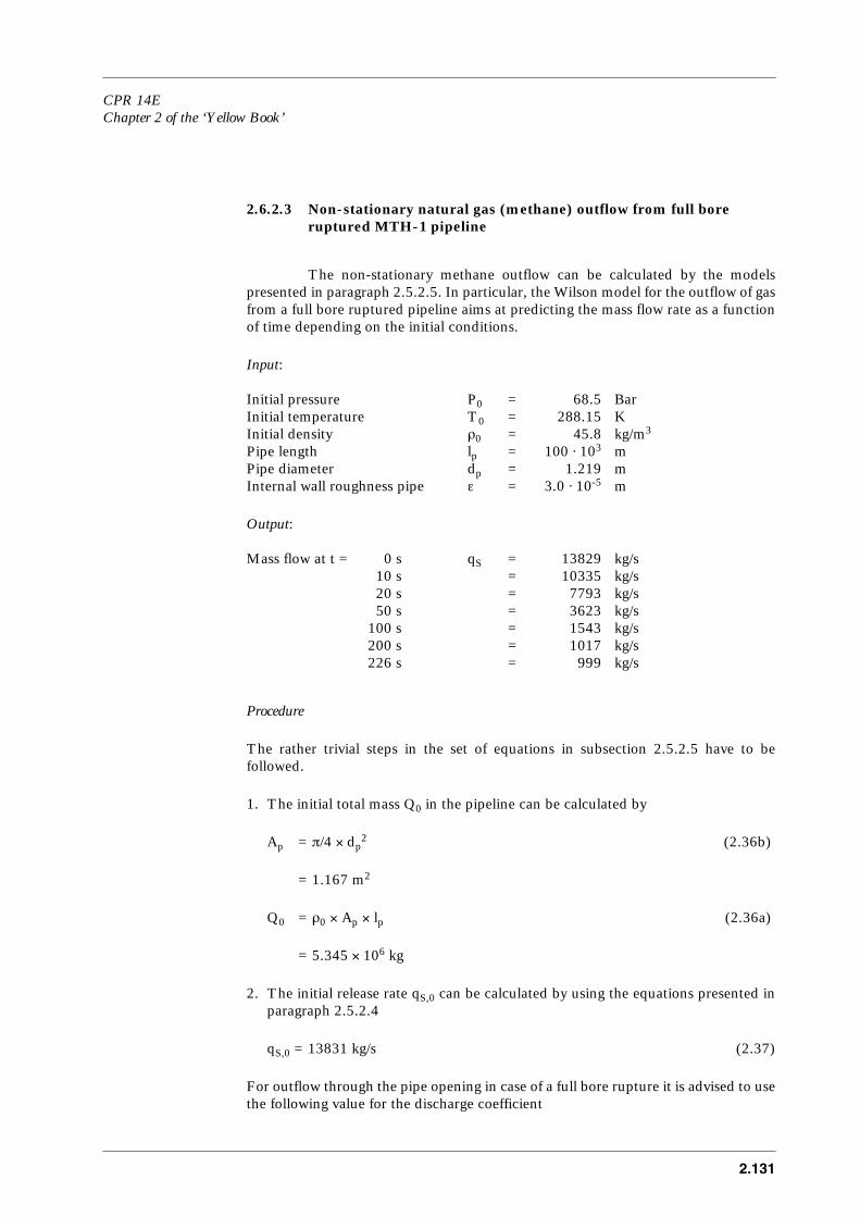
CPR 14EChapter 2 of the ‘Yellow Book’
2.131
2.6.2.3 Non-stationary natural gas (methane) outflow from full bore ruptured MTH-1 pipeline
The non-stationary methane outflow can be calculated by the modelspresented in paragraph 2.5.2.5. In particular, the Wilson model for the outflow of gasfrom a full bore ruptured pipeline aims at predicting the mass flow rate as a functionof time depending on the initial conditions.
Input:
Initial pressure P0 = 68.5 BarInitial temperature T0 = 288.15 KInitial density ρ0 = 45.8 kg/m3
Pipe length lp = 100 ⋅ 103 mPipe diameter dp = 1.219 mInternal wall roughness pipe ε = 3.0 ⋅ 10-5 m
Output:
Mass flow at t = 0 s qS = 13829 kg/s 10 s = 10335 kg/s 20 s = 7793 kg/s 50 s = 3623 kg/s100 s = 1543 kg/s200 s = 1017 kg/s226 s = 999 kg/s
Procedure
The rather trivial steps in the set of equations in subsection 2.5.2.5 have to befollowed.
1. The initial total mass Q0 in the pipeline can be calculated by
Ap = π/4 × dp2 (2.36b)
= 1.167 m2
Q0 = ρ0 × Ap × lp (2.36a)
= 5.345 × 10⁶ kg
2. The initial release rate qS,0 can be calculated by using the equations presented inparagraph 2.5.2.4
qS,0 = 13831 kg/s (2.37)
For outflow through the pipe opening in case of a full bore rupture it is advised to usethe following value for the discharge coefficient

2.132
Cd = 1.0 (2.38)
and ψ2 = 1 (2.24)
3. The sonic velocity in the gas us, assuming adiabatic expansion (∆S = 0), is givenfor perfect gases (z = 1, ζ = γ =1.31) and for methane (µi=16⋅10-3 kg/mol) by
(2.39c)
= 442.9 m/s
4. The Darcy friction factor may be calculated by the Von Karman equation
fD = 1./(-2 × 10log(ε/(3.715 × dp)))2 (2.40)
= 9.32 ⋅ 10-3
5. The time constant tB is given by
(2.41)
= 4764 sec
6. Finally the mass flow rate qS(t) can be estimated at any time t after the full borerupture of the pipeline by the Wilson model given by equation (2.35).
The mass flow rate for a full bore ruptured pipeline according to the model of Wilsonat t=100
qS(t)= qS,0/(1+Q0/(tB × qS,0)) × Q0/(tB × qS,0) × exp(-t/tB) + exp(-t × tB × (qS,0/Q0)2)
= 12793 kg/s × 7.944 ⋅ 10-2 + 4.118 ⋅ 10-2
= 1543 kg/s
7. Check the validity of the model.
When the pressure wave travelling upstream reaches the opposite side of the pipelinethe Wilson model is not valid any more. This occurs after
tE = lp/us (2.42)
= 1.00 ⋅ 105 m / 442.9 m/s
= 225.8 s
us ζ z R T0 µi⁄×××( )=
tB 2 3 lp us⁄×⁄ γ fD lp dp⁄××( )×=
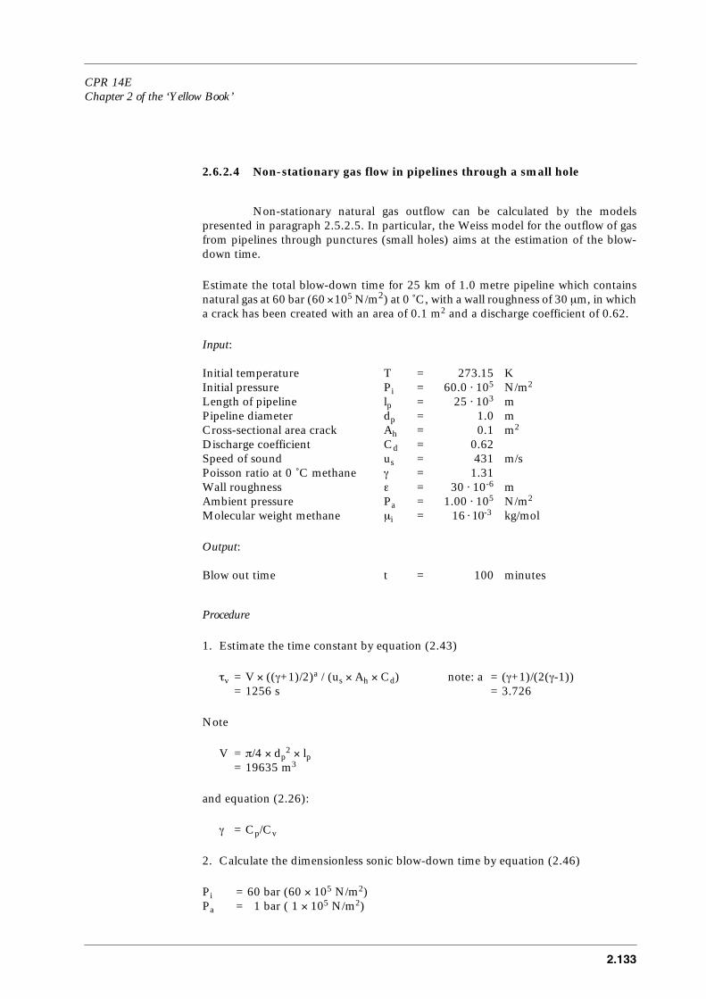
CPR 14EChapter 2 of the ‘Yellow Book’
2.133
2.6.2.4 Non-stationary gas flow in pipelines through a small hole
Non-stationary natural gas outflow can be calculated by the modelspresented in paragraph 2.5.2.5. In particular, the Weiss model for the outflow of gasfrom pipelines through punctures (small holes) aims at the estimation of the blow-down time.
Estimate the total blow-down time for 25 km of 1.0 metre pipeline which containsnatural gas at 60 bar (60 ×105 N/m2) at 0 C, with a wall roughness of 30 µm, in whicha crack has been created with an area of 0.1 m2 and a discharge coefficient of 0.62.
Input:
Initial temperature T = 273.15 KInitial pressure Pi = 60.0 ⋅ 105 N/m2
Length of pipeline lp = 25 ⋅ 103 mPipeline diameter dp = 1.0 mCross-sectional area crack Ah = 0.1 m2
Discharge coefficient Cd = 0.62Speed of sound us = 431 m/sPoisson ratio at 0 ˚C methane γ = 1.31Wall roughness ε = 30 ⋅ 10-6 m Ambient pressure Pa = 1.00 ⋅ 105 N/m2
Molecular weight methane µi = 16 ⋅ 10-3 kg/mol
Output:
Blow out time t = 100 minutes
Procedure
1. Estimate the time constant by equation (2.43)
τv = V × ((γ+1)/2)a / (us × Ah × Cd) note: a = (γ+1)/(2(γ-1))= 1256 s = 3.726
Note
V = π/4 × dp2 × lp
= 19635 m3
and equation (2.26):
γ = Cp/Cv
2. Calculate the dimensionless sonic blow-down time by equation (2.46)
Pi = 60 bar (60 × 105 N/m2)Pa = 1 bar ( 1 × 10⁵ N/m2)

2.134
So,
τcr = ln(Pi/Pa) - (γ/(γ-1)) × ln((γ+1)/2)
= 3.485
3. Calculate the dimensionless sub-sonic blow-down time by interpolating table 2.1
γ = 1.31
So,
τs = 0.79
4. Estimate the blow-down correction factor Cb by equations (2.48), (2.49), (2.50)and (2.51)
fD = 0.0964 (pipe wall roughness ε=0.00003)fD × lp/dp = 241Ap = π/4 × dp
2
= 0.785 m2
Ap/(Ah × Cd)= 12.67
So,
Cb = 1.12
5. Calculate the total blow-down time by equation (2.57)
t = (τcr+τs) × τv × Cb= (3.485+0.79) × 1256 × 1.12= 100 minutes
2.6.3 Pressurised liquefied gases
2.6.3.1 Champagne release of propane through a hole in the side-wall of vertical cylinder
Input:
Vessel volume Vv = 4.7 m3
Length cylinder lv = 2.0 m Filling degree φ = 0.95 m3/m3
Initial temperature T0 = 303.15 KLeak size dh = 0.1 mLeak height hh = 1.95 mDischarge coefficient Cd = 0.62
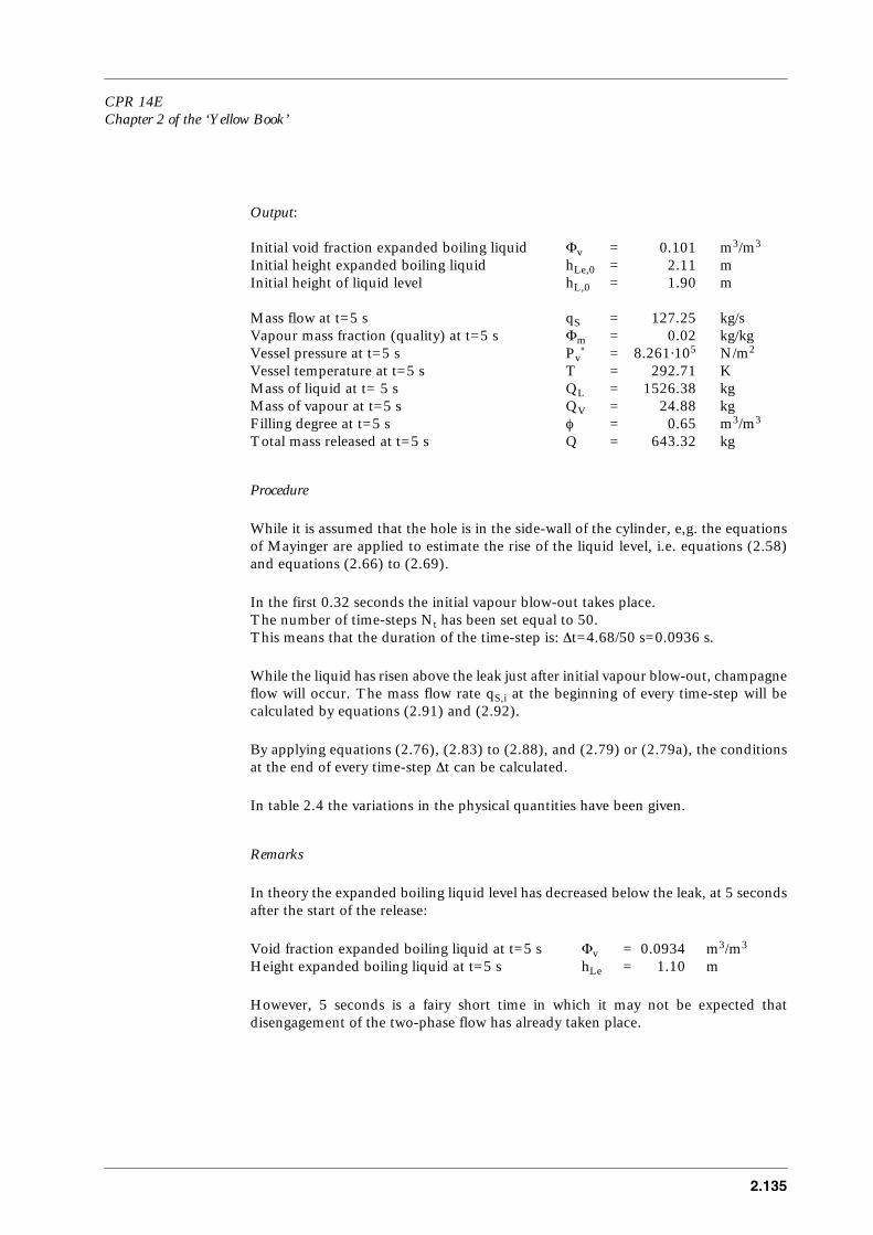
CPR 14EChapter 2 of the ‘Yellow Book’
2.135
Output:
Initial void fraction expanded boiling liquid Φv = 0.101 m3/m3
Initial height expanded boiling liquid hLe,0 = 2.11 m Initial height of liquid level hL,0 = 1.90 m
Mass flow at t=5 s qS = 127.25 kg/sVapour mass fraction (quality) at t=5 s Φm = 0.02 kg/kgVessel pressure at t=5 s Pv˚ = 8.261⋅105 N/m2
Vessel temperature at t=5 s T = 292.71 KMass of liquid at t= 5 s QL = 1526.38 kgMass of vapour at t=5 s QV = 24.88 kgFilling degree at t=5 s φ = 0.65 m3/m3
Total mass released at t=5 s Q = 643.32 kg
Procedure
While it is assumed that the hole is in the side-wall of the cylinder, e,g. the equationsof Mayinger are applied to estimate the rise of the liquid level, i.e. equations (2.58)and equations (2.66) to (2.69).
In the first 0.32 seconds the initial vapour blow-out takes place.The number of time-steps Nt has been set equal to 50.This means that the duration of the time-step is: ∆t=4.68/50 s=0.0936 s.
While the liquid has risen above the leak just after initial vapour blow-out, champagneflow will occur. The mass flow rate qS,i at the beginning of every time-step will becalculated by equations (2.91) and (2.92).
By applying equations (2.76), (2.83) to (2.88), and (2.79) or (2.79a), the conditionsat the end of every time-step ∆t can be calculated.
In table 2.4 the variations in the physical quantities have been given.
Remarks
In theory the expanded boiling liquid level has decreased below the leak, at 5 secondsafter the start of the release:
Void fraction expanded boiling liquid at t=5 s Φv = 0.0934 m3/m3
Height expanded boiling liquid at t=5 s hLe = 1.10 m
However, 5 seconds is a fairy short time in which it may not be expected thatdisengagement of the two-phase flow has already taken place.

2.136
Table 2.4
t qS T Φm,e φ QL QV Pv˚(T)
(s) (kg/s) (K) (kg/kg) (m3/m3) (kg) (kg) (N/m2)
0.00 13.92 303.15 0.0003 0.9500 2168.94 4.29 10.79⋅105
0.32 131.60 294.55 0.0017 0.9223 2165.26 3.68 8.67⋅105
0.41 131.27 294.40 0.0017 0.9155 2150.47 6.18 8.64⋅105
0.51 131.00 294.37 0.0029 0.9101 2137.81 6.58 8.63⋅105
0.60 130.89 294.35 0.0031 0.9046 2125.16 6.97 8.62⋅105
0.69 130.84 294.32 0.0033 0.8992 2112.51 7.37 8.62⋅105
0.79 130.78 294.29 0.0035 0.8937 2099.88 7.76 8.61⋅105
0.88 130.72 294.27 0.0037 0.8883 2087.24 8.15 8.61⋅105
0.97 130.67 294.24 0.0039 0.8828 2074.62 8.55 8.60⋅105
1.07 130.61 294.21 0.0041 0.8774 2062.00 8.94 8.59⋅105
1.16 130.55 294.19 0.0043 0.8719 2049.38 9.33 8.59⋅105
1.25 130.49 294.16 0.0045 0.8665 2036.78 9.72 8.58⋅105
1.35 130.43 294.13 0.0047 0.8611 2024.18 10.11 8.58⋅105
1.44 130.37 294.10 0.0050 0.8556 2011.58 10.49 8.57⋅105
1.54 130.31 294.08 0.0052 0.8502 1998.99 10.88 8.56⋅105
1.63 130.24 294.05 0.0054 0.8448 1986.41 11.27 8.56⋅105
1.72 130.18 294.02 0.0056 0.8393 1973.84 11.65 8.55⋅105
1.82 130.12 293.99 0.0059 0.8339 1961.27 12.04 8.54⋅105
1.91 130.05 293.96 0.0061 0.8285 1948.71 12.42 8.54⋅105
2.00 129.99 293.93 0.0063 0.8231 1936.16 12.81 8.53⋅105
2.10 129.92 293.90 0.0066 0.8177 1923.61 13.19 8.52⋅105
2.19 129.86 293.87 0.0068 0.8123 1911.07 13.57 8.52⋅105
2.28 129.79 293.84 0.0071 0.8069 1898.54 13.95 8.51⋅105
2.38 129.72 293.80 0.0073 0.8015 1886.01 14.33 8.50⋅105
2.47 129.65 293.77 0.0075 0.7961 1873.49 14.71 8.50⋅105
2.57 129.58 293.74 0.0078 0.7907 1860.98 15.09 8.49⋅105
2.66 129.51 293.71 0.0080 0.7853 1848.48 15.46 8.48⋅105
2.75 129.44 293.68 0.0083 0.7799 1835.98 15.84 8.47⋅105
2.85 129.37 293.64 0.0086 0.7745 1823.50 16.21 8.47⋅105
2.94 129.30 293.61 0.0088 0.7691 1811.02 16.59 8.46⋅105
3.03 129.22 293.57 0.0091 0.7638 1798.55 16.96 8.45⋅105
3.13 129.15 293.54 0.0093 0.7584 1786.08 17.33 8.44⋅105
3.22 129.07 293.51 0.0096 0.7530 1773.63 17.70 8.44⋅105
3.31 129.00 293.47 0.0099 0.7477 1761.18 18.07 8.43⋅105
3.41 128.92 293.43 0.0102 0.7423 1748.74 18.44 8.42⋅105
3.50 128.84 293.40 0.0104 0.7369 1736.31 18.81 8.41⋅105
3.60 128.76 293.36 0.0107 0.7316 1723.89 19.18 8.40⋅105
3.69 128.68 293.32 0.0110 0.7262 1711.47 19.54 8.40⋅105
3.78 128.60 293.29 0.0113 0.7209 1699.07 19.91 8.39⋅105
3.88 128.52 293.25 0.0116 0.7155 1686.67 20.27 8.38⋅105
3.97 128.43 293.21 0.0119 0.7102 1674.28 20.63 8.37⋅105
4.06 128.35 293.17 0.0122 0.7049 1661.91 20.99 8.36⋅105
4.16 128.26 293.13 0.0125 0.6995 1649.54 21.35 8.35⋅105
4.25 128.18 293.09 0.0128 0.6942 1637.18 21.71 8.35⋅105
4.34 128.09 293.05 0.0131 0.6889 1624.83 22.07 8.34⋅105
4.44 128.00 293.01 0.0134 0.6836 1612.49 22.42 8.33⋅105
4.53 127.91 292.97 0.0137 0.6783 1600.15 22.78 8.32⋅105
4.63 127.82 292.93 0.0140 0.6729 1587.83 23.13 8.31⋅105
4.72 127.73 292.88 0.0144 0.6676 1575.52 23.48 8.30⋅105
4.81 127.64 292.84 0.0147 0.6623 1563.22 23.83 8.29⋅105
4.91 127.54 292.80 0.0150 0.6570 1550.93 24.18 8.28⋅105
5.00 127.45 292.75 0.0154 0.6517 1538.65 24.53 8.27⋅105
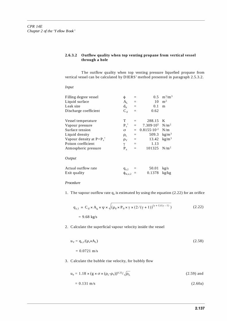
CPR 14EChapter 2 of the ‘Yellow Book’
2.137
2.6.3.2 Outflow quality when top venting propane from vertical vessel through a hole
The outflow quality when top venting pressure liquefied propane fromvertical vessel can be calculated by DIERS’ method presented in paragraph 2.5.3.2.
Input
Filling degree vessel φ = 0.5 m3/m3
Liquid surface AL = 10 m2
Leak size dh = 0.1 mDischarge coefficient Cd = 0.62
Vessel temperature T = 288.15 KVapour pressure Pv˚ = 7.309⋅105 N/m2
Surface tension σ = 0.8155⋅10-2 N/mLiquid density ρL = 509.3 kg/m3
Vapour density at P=Pv˚ ρV = 13.42 kg/m3
Poison coefficient γ = 1.13Atmospheric pressure Pa = 101325 N/m2
Output
Actual outflow rate qs,2 = 50.01 kg/sExit quality φm,e,2 = 0.1378 kg/kg
Procedure
1. The vapour outflow rate qs is estimated by using the equation (2.22) for an orifice
(2.22)
= 9.68 kg/s
2. Calculate the superficial vapour velocity inside the vessel
uV = qs,1/(ρv×AL) (2.58)
= 0.0721 m/s
3. Calculate the bubble rise velocity, for bubbly flow
ub = 1.18 × (g × σ × (ρL-ρV))0.25/ (2.59) and
= 0.131 m/s (2.60a)
qs ,1 Cd A× h ψ ρ0 P0 γ 2 γ 1+( )⁄( ) γ 1+( )/ γ 1–( )×××( )××=
ρL

2.138
and for churn flow
ub = 1.53 × (g × σ × (ρL-ρV))0.25/ (2.59) and
= 0.170 m/s (2.60b)
4. The dimensionless superficial vapour velocity is given by
uVR = uV/ub (2.61)
So, for bubbly flow
uVR = 0.549 m/s
and for churn flow
uVR = 0.424 m/s
5. Calculate the characteristic dimensionless superficial velocity uVR for both typicaltwo-phase flow types.
The void fraction in the vessel can be calculated by
Φv = 1 - φ (2.63)
= 0.5 m3/m3
uVR,bf = Φv × (1-Φv)2/((1- ) × (1-1.2 × Φv)) (2.62a,b)
= 0.357 m/s
uVR,cf = 2 × Φv/(1-1.5 × Φv) (2.62c,d)
= 4.00 m/s
ρL
Φv3

CPR 14EChapter 2 of the ‘Yellow Book’
2.139
6. Determination whether two-phase flow is apparent inside the vessel
Application the of criteria
uVR < uVR,cf → no churn flow (2.64c)
uVR ≥ uVR,bf → two-phase bubbly flow (2.64b)
7. The exit quality and outflow rate can be calculated by solving the set of equations(2.65), (2.65a) and (2.65b). The iteration can be carried out by a root findingprocedure.
For two-phase flow through a hole, the outflow rate can be calculated by
qs,2 = Cd × A × (2.91)
withρav = 1 / (Φm/ρV + (1-Φm)/ρL) (2.92)
The actual outflow rate qs,2 is given above at “Output”.
2.6.3.3 Stationary two-phase propane flow through full bore ruptured pipe
The stationary outflow of two-phase propane flow from a pipeline can becalculated by the TPDIS model presented in paragraph 2.5.3.5.
Input:
Pipe length lp = 100.0 mPipe diameter dp = 0.1 mWall roughness pipe ε = 4.5⋅10-5 mConstant up-stream temperature T0 = 288.15 KDischarge coefficient Cd = 1.0
Output:
Mass flow rate qS = 16.35 kg/sVapour mass fraction (quality) Φm,e = 0.0621 kg/kgExit temperature Te = 279.4 KConstant up-stream pressure Pv˚(T0) = 7.309⋅105 N/m2
2 P0 Pa–( ) ρav×( )
2.140
Procedure
The critical mass flow rate qs(Pe) at the pipe outlet may be computed by numericallymaximising the right-hand side of equation (2.107) in terms of outlet pressure Pe.The specific volume of the liquid is computed by equations (2.110) and (2.112).The friction is computed by equation (2.99), using the mass flow rate estimated inthe previous step.Note that SL(P0) = 4.39⋅103 J/(kg⋅K), and the values for the following parameters:CAr=0.5, CBr=0.5.
2.6.3.4 Non-stationary two-phase flow in pipelines
The modelling of the two-phase flow through pipelines aims at predictingthe mass flow rate as a function of time depending on the initial conditions.
Transient release from full bore ruptured pipelines
Non-stationary two-phase outflow through pipelines can be calculated by the modelspresented in paragraph 2.5.3.6.Morrow’s model can be used to estimate the mass flow rate caused by a full boreruptured propane-pipeline as a function of time.
Problem
A pipeline filled with propane is ruptured in the middle. Calculate the transient massflow rate as a function of time after the rupture.
Input:
Initial pipeline pressure P0 = 60⋅105 N/m2
Initial temperature T0 = 288.15 KPipe length Lp = 50⋅103 mPipe diameter dp = 0.254 m(cross-sectional area Ap = 0.05067 m2)Sound speed in propane liquid us,L = 864.9 m/s
Output:
Mass flow at 0 sec qS,e = 672.3 kg/sQuality at 0 sec Φm = 0.195 kg/kg
Mass flow at 4990 sec qS,e = 70.37 kg/sQuality at 4990 sec Φm = 0.298 kg/kg
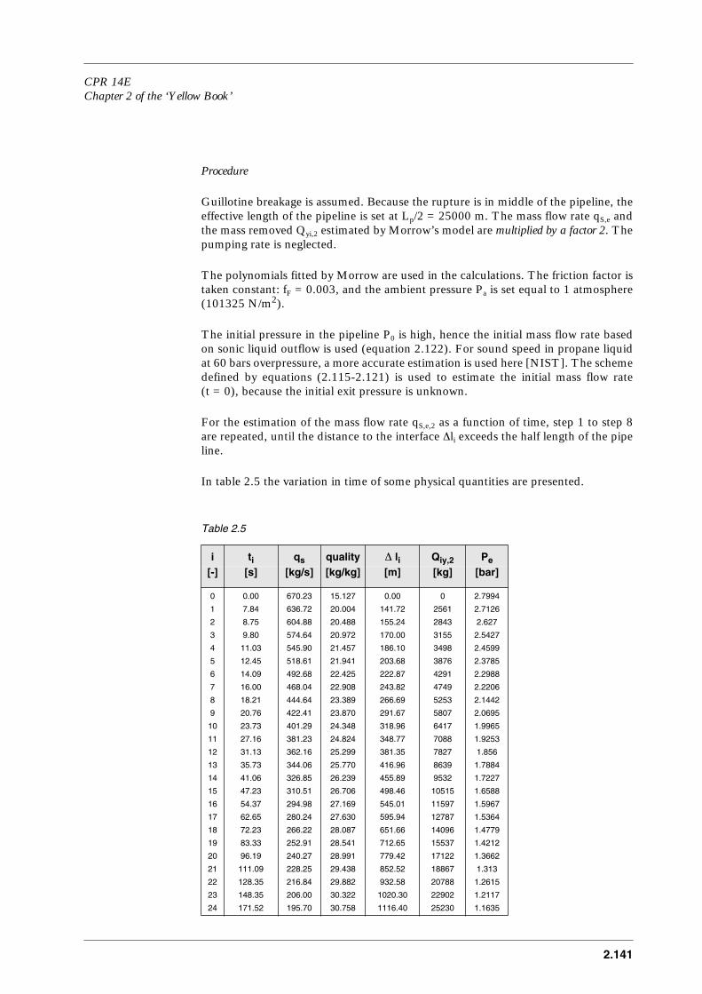
CPR 14EChapter 2 of the ‘Yellow Book’
2.141
Procedure
Guillotine breakage is assumed. Because the rupture is in middle of the pipeline, theeffective length of the pipeline is set at Lp/2 = 25000 m. The mass flow rate qS,e andthe mass removed Qyi,2 estimated by Morrow’s model are multiplied by a factor 2. Thepumping rate is neglected.
The polynomials fitted by Morrow are used in the calculations. The friction factor istaken constant: fF = 0.003, and the ambient pressure Pa is set equal to 1 atmosphere(101325 N/m2).
The initial pressure in the pipeline P0 is high, hence the initial mass flow rate basedon sonic liquid outflow is used (equation 2.122). For sound speed in propane liquidat 60 bars overpressure, a more accurate estimation is used here [NIST]. The schemedefined by equations (2.115-2.121) is used to estimate the initial mass flow rate(t = 0), because the initial exit pressure is unknown.
For the estimation of the mass flow rate qS,e,2 as a function of time, step 1 to step 8are repeated, until the distance to the interface ∆li exceeds the half length of the pipeline.
In table 2.5 the variation in time of some physical quantities are presented.
Table 2.5
i ti qs quality ∆ li Qiy,2 Pe
[-] [s] [kg/s] [kg/kg] [m] [kg] [bar]
0 0.00 670.23 15.127 0.00 0 2.7994
1 7.84 636.72 20.004 141.72 2561 2.7126
2 8.75 604.88 20.488 155.24 2843 2.627
3 9.80 574.64 20.972 170.00 3155 2.5427
4 11.03 545.90 21.457 186.10 3498 2.4599
5 12.45 518.61 21.941 203.68 3876 2.3785
6 14.09 492.68 22.425 222.87 4291 2.2988
7 16.00 468.04 22.908 243.82 4749 2.2206
8 18.21 444.64 23.389 266.69 5253 2.1442
9 20.76 422.41 23.870 291.67 5807 2.0695
10 23.73 401.29 24.348 318.96 6417 1.9965
11 27.16 381.23 24.824 348.77 7088 1.9253
12 31.13 362.16 25.299 381.35 7827 1.856
13 35.73 344.06 25.770 416.96 8639 1.7884
14 41.06 326.85 26.239 455.89 9532 1.7227
15 47.23 310.51 26.706 498.46 10515 1.6588
16 54.37 294.98 27.169 545.01 11597 1.5967
17 62.65 280.24 27.630 595.94 12787 1.5364
18 72.23 266.22 28.087 651.66 14096 1.4779
19 83.33 252.91 28.541 712.65 15537 1.4212
20 96.19 240.27 28.991 779.42 17122 1.3662
21 111.09 228.25 29.438 852.52 18867 1.313
22 128.35 216.84 29.882 932.58 20788 1.2615
23 148.35 206.00 30.322 1020.30 22902 1.2117
24 171.52 195.70 30.758 1116.40 25230 1.1635
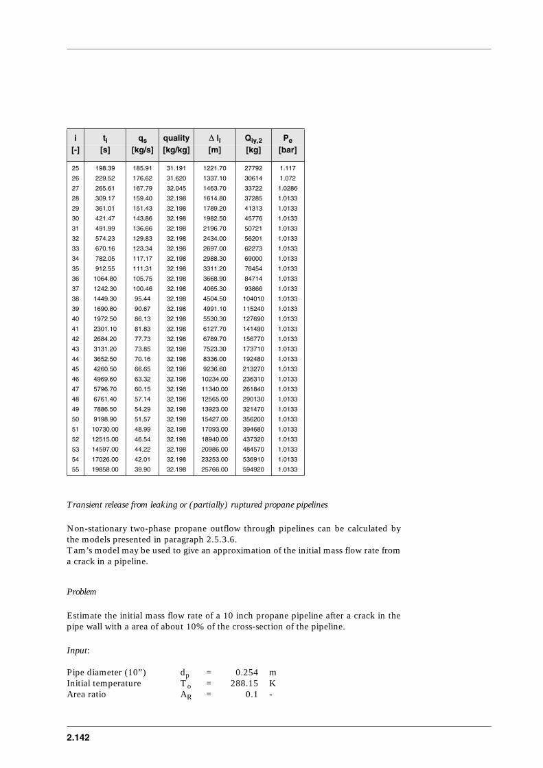
2.142
Transient release from leaking or (partially) ruptured propane pipelines
Non-stationary two-phase propane outflow through pipelines can be calculated bythe models presented in paragraph 2.5.3.6.Tam’s model may be used to give an approximation of the initial mass flow rate froma crack in a pipeline.
Problem
Estimate the initial mass flow rate of a 10 inch propane pipeline after a crack in thepipe wall with a area of about 10% of the cross-section of the pipeline.
Input:
Pipe diameter (10”) dp = 0.254 m Initial temperature To = 288.15 KArea ratio AR = 0.1 -
25 198.39 185.91 31.191 1221.70 27792 1.117
26 229.52 176.62 31.620 1337.10 30614 1.072
27 265.61 167.79 32.045 1463.70 33722 1.0286
28 309.17 159.40 32.198 1614.80 37285 1.0133
29 361.01 151.43 32.198 1789.20 41313 1.0133
30 421.47 143.86 32.198 1982.50 45776 1.0133
31 491.99 136.66 32.198 2196.70 50721 1.0133
32 574.23 129.83 32.198 2434.00 56201 1.0133
33 670.16 123.34 32.198 2697.00 62273 1.0133
34 782.05 117.17 32.198 2988.30 69000 1.0133
35 912.55 111.31 32.198 3311.20 76454 1.0133
36 1064.80 105.75 32.198 3668.90 84714 1.0133
37 1242.30 100.46 32.198 4065.30 93866 1.0133
38 1449.30 95.44 32.198 4504.50 104010 1.0133
39 1690.80 90.67 32.198 4991.10 115240 1.0133
40 1972.50 86.13 32.198 5530.30 127690 1.0133
41 2301.10 81.83 32.198 6127.70 141490 1.0133
42 2684.20 77.73 32.198 6789.70 156770 1.0133
43 3131.20 73.85 32.198 7523.30 173710 1.0133
44 3652.50 70.16 32.198 8336.00 192480 1.0133
45 4260.50 66.65 32.198 9236.60 213270 1.0133
46 4969.60 63.32 32.198 10234.00 236310 1.0133
47 5796.70 60.15 32.198 11340.00 261840 1.0133
48 6761.40 57.14 32.198 12565.00 290130 1.0133
49 7886.50 54.29 32.198 13923.00 321470 1.0133
50 9198.90 51.57 32.198 15427.00 356200 1.0133
51 10730.00 48.99 32.198 17093.00 394680 1.0133
52 12515.00 46.54 32.198 18940.00 437320 1.0133
53 14597.00 44.22 32.198 20986.00 484570 1.0133
54 17026.00 42.01 32.198 23253.00 536910 1.0133
55 19858.00 39.90 32.198 25766.00 594920 1.0133
i ti qs quality ∆ li Qiy,2 Pe
[-] [s] [kg/s] [kg/kg] [m] [kg] [bar]

CPR 14EChapter 2 of the ‘Yellow Book’
2.143
Output:
Initial mass flow qS = 69.4 kg/s
Procedure
The density of propane at initial temperature T0=15 ˚C (288.15 K) is
ρL,0 = 509.5 kg/m3
The radius ratio dR is given by
dR = dp[m] / 0.05 m
= 0.254m / 0.05 m
= 5.08
The area ratio has been given
AR = 0.1
So, the decay coefficient can be estimated by
Cα = dR0.25 × (0.22 × AR - 0.13 × AR
1.5 + 0.00068 × (T0-288.15)) (2.134)
= (5.08)0.25 × (0.22 × 0.1 - 0.13 × 0.11.5 + 0.)
= 0.0269 s-1
The (artificially) constant is set at
CLp = 100 m (2.137a)
The initial flow rate is given by
q0 = Cα × ρL,0 × π/4 × dp2 × CLp (2.137)
= 0.0269 × 509.5 × π/4 × 0.2542 × 100
= 69.4 kg/s
2.6.3.5 Finite duration spray releases
In order to demonstrate the calculation of a finite duration flashing release,the following situation has been selected: A 1000 m3 vessel is filled (fill level 50%)with butane at ambient temperature (288.15 K). At the bottom of the vessel a 3"

2.144
pipeline (76.2 mm diameter) is connected. 10 cm from the vessel connection, thispipeline breaks off completely. The breach is 1 m above the ground. This results in arelease of butane at a mass flow of about 41 kg s-1. The discharge coefficient is 0.8,so the effective exit area is 0.00365 m2. The flashing in the short pipe is negligible, sopure liquid flows out which flashes in the atmosphere. For the ambient humidity avalue of 63% is assumed. The input data and intermediate and final results aresummarised in Table 2.6.
Table 2.6 Input and output of the finite duration spray release example
Input Source heightEffective exit areaExit radiusMass flow rateVapour mass fractionExit temperatureExit pressureLiquid densityVapour densityAveraged densityExit velocityBoiling temperatureLatent heat
Vapour enthalpy
Ambient humidityAmbient temperature
hsAebeqS,eΦm,eTePeρe,Lρe,VρeueTBLv,eLv,fHe,VHf,VRHTa
10.003630.03441.340%288.15174549584.494.233584.4919.475272.736214037674047362242880663%288.15
mm2
mkg/s
KPakg/m3
kg/m3
kg/m3
m/sKJ/kgJ/kgJ/kgJ/kg
K
Afterflashing
Vapour mass fractionJet velocityLiquid densityVapour densityAveraged densityJet areaJet radius
Φm,fufρf,Lρf,VρfAfbf
0.1573225.91600.722.596416.130.0990.177
m/skg/m3
kg/m3
kg/m3
m2
m
Droplet diameter
Dynamic viscosity liquidSurface tensionJet Reynolds numberJet Weber numberDroplet diameter
νLσsRefWefdd
0.0001970.01594664890123390.29
N.s/m2
N/m
mm
Rain-out Kinematic viscosity airPrandtl number for airSchmidt number for butaneDroplet Reynolds numberFree fall velocityDroplet temperatureEvaporation coefficientNett mass released to the airNett vapour mass fraction Nett jet areaNett jet radius
νaPrScRedudTdkBqS,nett,airΦm,rainoutAf,rainoutbf,rainout
1.71·10-5
0.870.722.251.313215.092.87·10-8
41.340.157320.0990.177
m2/s
m/sKm2/skg/s
m2
m
Conditions after evaporation
Concentration after evaporationTemperature after evaporationMolar fraction of water vapour at ambient temperatureMolar fraction of water vapour at jet temperatureMolar fraction of condensed waterJet density after evaporationJet velocity after evaporationJet area after evaporationJet radius after evaporation
cjTjcw
cwv cjLρjujAjbj
0.138227.310.61
1.1582.445.1276.291.280.64
K
kg/m3
m/sm2
m
CPR 14EChapter 2 of the ‘Yellow Book’
2.145
The input listed in Table 2.6 includes the thermodynamic properties at the storageand boiling temperature: latent heat and the enthalpies (only enthalpy differencesbetween two temperatures and pressure levels are essential) as well as the densities.
Step 1 - Calculate the conditions in the jet after flashing
The outflow conditions Pe, Te, qS,e and Φm,e are listed in the Table 2.6. The densityat the exit follows from formula (2.138) (this formula will be used frequently tocalculate the density of two-phase mixtures at various stages throughout the jet):
(m3/kg)
ρe = 584.49 kg/m3
The jet velocity after flashing is calculated by formula (2.139):
(m/s)
uf = 25.91 m/s.
The vapour mass fraction after flashing is calculated by formula (2.140):
(-)
Φm,f = 0.15732
The jet cross section Af and jet radius bf can be calculated from (2.141).Here we need the averaged density ρf in the vessel, which can be calculated byformulae (2.138) from the vapour and liquid densities and the vapour mass fractionafter flashing.
(m2; m)
Af = 0.099 m2 ; bf=0.177 m.
1ρe-----
1 Φ– m e,( )
ρL e,------------------------
Φm e,
ρv e,-----------+=
ufPe Pa–( )Ae
qs e,--------------------------- ue+=
Φm f, 1HV f, HV e, 1 Φm e,+( )Lv e,
1
2-- uf
2 ue2–( )++–
Lv f,-------------------------------------------------------------------------------------------------–=
Af
ρeue
ρfuf---------- Ae bf
Af
π-----= =
2.146
Step 2 - Calculation of the droplet diameter after flashing
Next, the droplet diameter after flashing is calculated. First, the jet Reynolds numberand the jet Weber number are evaluated using formula (2.142):
(- ; -)
Ref = 46648Wef = 9012339
Then the droplet diameter is calculated by formulae (2.143a-b). It appears that in thiscase the second option (b) has to be used:
(m)
dd = 0.29 mm
Step 3 - Droplet evaporation and rain-out on the ground
Knowing the droplet diameter, it is possible to determine whether the droplets willfall on the ground. Therefore the free fall velocity of the droplet is estimated byformula (2.145).
(m/s)
ud = 1.313 m/s
This allows to evaluate the droplet Reynolds number Red.
Red = uddd/νRed = 22.25
Table 2.6 presents the values for the Schmidt and Prandtl numbers which depend onthe properties of butane and air only. In order to determine the evaporation coefficient kB (2.146), it is necessary todetermine the droplet temperature Td (2.147) in an iterative process usingintermediate values of kB at each iteration step. This results in Td = 215 K,kB = 2.87⋅10-8 m2/s.The approximate formula (2.148) for the maximum droplet diameter dM results in amaximum droplet of 47 mm. However, this is not a useful result, as the correspondingReynolds number using the free fall velocity, is 3671, which exceeds the range ofvalidity (Red < 4). Therefore it can not be avoided to integrate the differential equation (2.149) for theevolution of the droplet radius together with the descent of the droplet from therelease height to the ground (2.150):
Ref
2bfuf
νL------------ Wef
2bfuf2ρL f,
σs----------------------= =
dd 15σs
uf2ρa
----------=
ud
ρL f, g
18νaρa
----------------dd2=
CPR 14EChapter 2 of the ‘Yellow Book’
2.147
(m/s)
And found is that all droplets have evaporated before reaching the ground.
By means of formulae (2.151) to (2.153) the values of the airborne mass flow rate,vapour mass fraction, jet area and jet radius can be corrected for rain-out:
(kg/s)
qS,nett,air = 41.34 kg/s
(-)
Φm,f,rainout = 0.15732
(m2)
Af,rainout = 0.099 m2
bf,rainout = 0.177 m
Step 4 - Calculate the conditions in the jet after evaporation of all airbornedroplets
Finally, the effects of evaporation of droplets by entrained air on the bulk propertiesof the jet are calculated. Therefore, the enthalpy changes corresponding to thetemperature change and droplet evaporation of butane. The temperature change ofentrained air and the enthalpy change of ambient water, both due to condensationand temperature change, need to be calculated. This has to be done iteratively.Therefore an initial value of the jet temperature Tj is selected. A partial vapourpressure of butane corresponds to this temperature, and this leads to the molarfraction of butane in the jet by formula (2.155). Here we used:
logPs(Tj)=6.80896 - 935.860/(Tj + 238.73)
ddt-----dd
kB
dd----- 1 0.28 Red
1 2/ Sc1 3/+[ ]–=
0 h t0( ) hs ud td0
to
∫–= =
qs nett air,, Φm f, qs e, 1 Φm f,–( ) 1d0
dd-----
3
– qs e,+=
Φm f rainout, ,
Φm f,
Φm f, 1 Φm f,–( ) 1d0
dd
-----3
– +
------------------------------------------------------------------=
Af rainout, Af
qs nett air,,
qs e,--------------------=
2.148
With this information the enthalpy change of butane is calculated by (2.156). Thelatent heat after flashing Lv,f is listed in Table 2.6. The vapour enthalpy is calculatedfrom Cp⋅T, with:
Cp = -1.779 + 0.386961 × T - 193.255 × 10⁻⁶ × T2 + 348.326 × 10⁻¹⁰ × T3
Ambient humidity is transferred into a water mass fraction by using the relationbetween the saturation pressure of water as a function of temperature:
(-)
(-)
cw = 10.61
At the selected jet temperature this may lead to condensation: the remaining watervapour is calculated by means of (2.158). Now the enthalpy changes of dry air andwater can be calculated using (2.160) and (2.161), respectively. This process needsto be repeated until a jet temperature is reached at which the sum of the enthalpychanges is approximately zero. In this case one should find Tj = 227.3 K. Table 2.6presents the results as well as some thermodynamic properties at the final result forTj in this case.
Knowing the molar concentration, the amount of condensed water and thetemperature, it is possible to calculate jet density, jet velocity and jet dimensions byformulae (2.162) through (2.167):
(-)
cjL = 2.44
(kg/mol)
(kg/m3)
(kg/m3)
ρj = 5.127 (using ρj,L= 1000 kg/m3)The initial volume concentration in the volume flow rate is cj = 0.138:
(m/s)
mw
mda---------
RHaPv w,0 Ta( )
R µw⁄( )Ta ρa--------------------------------=
cwmwµa
mdaµw---------------=
cjL
1 cj–( )
1 cwv+( )-------------------- cw cwv–( )
µw
µjd------=
µjd cjµs
1 cj–( )
1 cwv–( )-------------------- µa cwv µw+( )+=
ρjdPa µjd
RTj--------------=
ρj1 cjL+
1ρj d,--------
cjL
ρw L,----------+
-------------------------=
ujuf
11 cj–( )
cj----------------
µa
µs-----+
------------------------------=
CPR 14EChapter 2 of the ‘Yellow Book’
2.149
uj = 6.29 m/s
(m2; m)
Aj = 1.28 m2
bj = 0.64 m
2.6.3.6 Instantaneous release
In order to demonstrate the calculation of an instantaneous flashing release,the following situation has been selected: A vessel is filled (fill level about 94%) with6 tonnes of propane at ambient temperature (291 K). This vessel fails completely.The ambient conditions are wind speed at 10 m height: 4 m/s, roughness length 0.03m (Flat land) and Monin-Obukhov length -21.7 m (sunny weather, slightly unstable:this meteorological condition is described in chapter 4, section 4.6.2.1). For theambient humidity a value of 63% is assumed. The input data and intermediate andfinal results are summarised in Table 2.7.
Aj
ρfuf
ρjuj--------- Af bj
Aj
π-----= =
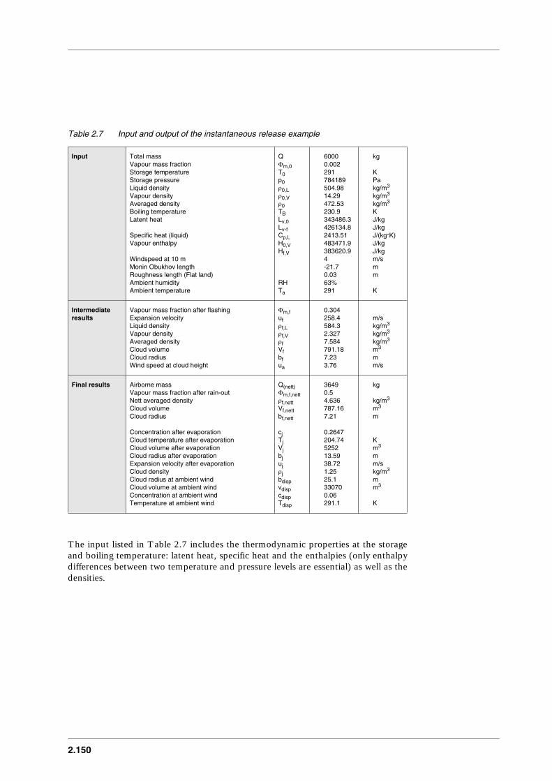
2.150
Table 2.7 Input and output of the instantaneous release example
The input listed in Table 2.7 includes the thermodynamic properties at the storageand boiling temperature: latent heat, specific heat and the enthalpies (only enthalpydifferences between two temperature and pressure levels are essential) as well as thedensities.
Input Total massVapour mass fractionStorage temperatureStorage pressureLiquid densityVapour densityAveraged densityBoiling temperatureLatent heat
Specific heat (liquid)Vapour enthalpy
Windspeed at 10 mMonin Obukhov lengthRoughness length (Flat land)Ambient humidityAmbient temperature
QΦm,0T0p0ρ0,Lρ0,Vρ0TBLv,0Lv,fCp,LH0,VHf,V
RHTa
60000.002291784189504.9814.29472.53230.9343486.3426134.82413.51483471.9383620.94-21.70.0363%291
kg
KPakg/m3
kg/m3
kg/m3
KJ/kgJ/kgJ/(kg⋅K)J/kgJ/kgm/smm
K
Intermediate results
Vapour mass fraction after flashingExpansion velocityLiquid densityVapour densityAveraged densityCloud volumeCloud radiusWind speed at cloud height
Φm,fufρf,Lρf,VρfVfbfua
0.304258.4584.32.3277.584791.187.233.76
m/skg/m3
kg/m3
kg/m3
m3
mm/s
Final results Airborne massVapour mass fraction after rain-outNett averaged densityCloud volumeCloud radius
Concentration after evaporationCloud temperature after evaporationCloud volume after evaporationCloud radius after evaporationExpansion velocity after evaporationCloud densityCloud radius at ambient windCloud volume at ambient windConcentration at ambient windTemperature at ambient wind
Q(nett)Φm,f,nettρf,nettVf,nettbf,nett
cjTjVjbjujρjbdispvdispcdispTdisp
36490.54.636787.167.21
0.2647204.74525213.5938.721.2525.1330700.06291.1
kg
kg/m3
m3
m
Km3
mm/skg/m3
mm3
K
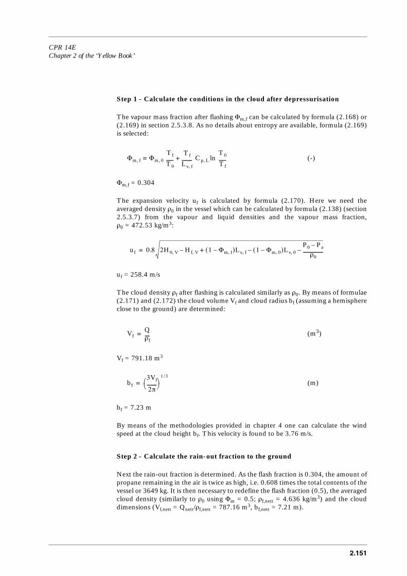
CPR 14EChapter 2 of the ‘Yellow Book’
2.151
Step 1 - Calculate the conditions in the cloud after depressurisation
The vapour mass fraction after flashing Φm,f can be calculated by formula (2.168) or(2.169) in section 2.5.3.8. As no details about entropy are available, formula (2.169)is selected:
(-)
Φm,f = 0.304
The expansion velocity uf is calculated by formula (2.170). Here we need theaveraged density ρ0 in the vessel which can be calculated by formula (2.138) (section2.5.3.7) from the vapour and liquid densities and the vapour mass fraction,ρ0 = 472.53 kg/m3:
uf = 258.4 m/s
The cloud density ρf after flashing is calculated similarly as ρ0. By means of formulae(2.171) and (2.172) the cloud volume Vf and cloud radius bf (assuming a hemisphereclose to the ground) are determined:
(m3)
Vf = 791.18 m3
(m)
bf = 7.23 m
By means of the methodologies provided in chapter 4 one can calculate the windspeed at the cloud height bf. This velocity is found to be 3.76 m/s.
Step 2 - Calculate the rain-out fraction to the ground
Next the rain-out fraction is determined. As the flash fraction is 0.304, the amount ofpropane remaining in the air is twice as high, i.e. 0.608 times the total contents of thevessel or 3649 kg. It is then necessary to redefine the flash fraction (0.5), the averagedcloud density (similarly to ρ0 using Φm = 0.5; ρf,nett = 4.636 kg/m3) and the clouddimensions (Vf,nett = Qnett/ρf,nett = 787.16 m3, bf,nett = 7.21 m).
Φm f, Φm 0,= Tf
T0------
Tf
Lv f,--------+ Cp L,
T0
Tf------ln
uf 0.8 2H0 V, Hf V, 1 Φm f,–( )Lv f, 1 Φm 0,–( )Lv 0,
P0 Pa–
ρ0----------------––+–=
VfQρf----=
bf
3Vf
2π--------
1 3/
=

2.152
Steps 3/4 Calculate the expansion of the cloud during the entrainmentphase and calculate the conditions in the cloud after evaporationof all airborne droplets
The amount of air that needs to be entrained in order to evaporate all propanedroplets in the cloud, is now calculated iteratively by means of formulae (2.154) to(2.161) from section 2.5.3.7. This will give the molar fraction of propane in the cloudcj, the cloud temperature Tj and the mass fraction of water droplets due tocondensation of ambient humidity. From this, one can also calculate the clouddensity ρj by formulae (2.162) to (2.167). This procedure has already beendemonstrated more extensively in the foregoing section. The results are presented inTable 2.7.In order to calculate the cloud volume it is necessary to calculate the vapour densityof the chemical at temperature Tj, ρs,j. In this case at 204.74 K the density of propaneis assumed to be 2.625 kg/m3. The cloud volume and radius follow from:
(m3; m)
Vj = 5252 m3 ; bj = 13.59 m
The expansion velocity of the cloud after evaporation follows from formula (2.175):uj = uf (bf/bj)
3
uj = 38.72 m/s
It appears that after evaporation the expansion velocity exceeds the ambient windspeed (38.72 m/s compared to 3.76 m/s). Therefore the cloud dimensions arecalculated when the expansion velocity equals the ambient wind speed by:
(m; m3)
bdisp = 25.1 m ; vdisp = 33070 m3
After the cloud has expanded to these dimensions, the temperature in the cloud Tc isapproaching the ambient temperature according to:
(K)
Tdisp = 291.1 K
The molar or volume concentration cdisp at this stage of the cloud is:
(-)
VjQ
cj ρs j,------------- bj
3Vj
2π--------
1 3/
= =
bdisp bf= uf
ua bf( )--------------
1 3/ Vdisp
2
3--πbdisp
3=
TdispTa
1 Vj
Vdisp----------- 1 Ta
Tj------
– –
----------------------------------------=
cdisp cj= VjTdisp
VdispTj-----------------

CPR 14EChapter 2 of the ‘Yellow Book’
2.153
cdisp = 0.06
The cloud density, calculated by means of (2.162) and (2.163) from section 2.5.3.4,is 1.25 kg/m3, which is about equal to the density of air at 15˚C (288.15 K).
2.6.4 Liquids
2.6.4.1 Stationary Acrylonitrile liquid outflow from a vessel through a hole in the vessel wall
The liquid outflow from of a vessel through a hole in the vessel wall can becalculated by the models presented in paragraphs 2.5.4.1 and 2.5.4.2.
Input:
Vessel volume V = 6600 m3
Vessel type vertical cylinderLength cylinder lv = 14 mFilling degree φ = 0.8 -Pressure above liquid p = 101325 N/m2
Leak size dh = 0.1 mHeight of leak hh = 0 mInitial temperature T0 = 288.15 KDischarge coefficient Cd = 0.62 -
Output:
Mass flow liquid at 500 sec qS = 58.44 kg/sFilling degree at 500 sec φ = 0.795 -Height of liquid at 500 sec hL = 11.12 mTotal mass released at 500 sec Q = 29416 kg
Procedure
The number of time-steps Nt has been set equal to 50.By equation (2.194), the mass flow rate qs,i at the beginning of every time-step can becalculated.
Using the equations (2.185) to (2.191) subsequently, the variation of the vesselconditions (Qi, hL,i) due to the outflow can be calculated.Note that the initial liquid mass in the tank is Q0, and that at a temperature ofT=15 ˚C (288.15) the density ρL of acrylonitrile are respectively
Q0(t=0) = 4290000 kg
ρL = 812.5 kg/m3
In table 2.8 the variations in the physical quantities have been given.

2.154
Table 2.8
Time after rupture
Mass flow rate
Fillingdegree
Total mass release
Liquid level in the vessel
[s] [kg/s] [%] [kg] [m]
0 60.915 80 0 11.20
2013 60.075 77.8 121790 10.89
4698 58.955 74.9 281550 10.49
7382 57.835 72.1 438300 10.10
10066 56.714 69.3 592050 9.71
12751 55.594 66.6 742790 9.33
15435 54.474 64.0 890520 8.96
18119 53.353 61.4 1035200 8.59
20804 52.233 58.8 1177000 8.23
23488 51.112 56.3 1315700 7.89
26172 49.991 53.9 1451400 7.54
28857 48.871 51.5 1584100 7.21
31541 47.750 49.2 1713700 6.88
34226 46.629 46.9 1840400 6.56
36910 45.508 44.7 1964100 6.25
39594 44.387 42.5 2084700 5.95
42279 43.266 40.4 2202400 5.65
44963 42.145 38.3 2317000 5.36
47647 41.023 36.3 2428600 5.08
50332 39.902 34.3 2537300 4.81
53016 38.780 32.4 2642900 4.54
55700 37.659 30.6 2745500 4.28
58385 36.537 28.8 2845000 4.03
61069 35.415 27.0 2941600 3.79
63753 34.293 25.4 3035200 3.55
66438 33.171 23.7 3125700 3.32
69122 32.049 22.1 3213300 3.10
71806 30.926 20.6 3297800 2.89
74491 29.803 19.2 3379300 2.68
77175 28.680 17.7 3457800 2.48
79860 27.557 16.4 3533300 2.29
82544 26.434 15.1 3605700 2.11
85228 25.310 13.8 3675200 1.93
87913 24.186 12.6 3741600 1.77
90597 23.062 11.5 3805000 1.61
93281 21.938 10.4 3865400 1.45
95966 20.813 9.3 3922800 1.31
98650 19.687 8.4 3977200 1.17
101330 18.562 7.4 4028500 1.04
104020 17.435 6.6 4076800 0.92
106700 16.308 5.7 4122100 0.80
109390 15.181 5.0 4164400 0.70
112070 14.053 4.3 4203600 0.60
114760 12.923 3.6 4239800 0.50
117440 11.793 3.0 4273000 0.42
120120 10.661 2.5 4303100 0.34
122810 9.528 2.0 4330200 0.27
125490 8.393 1.5 4354300 0.21
128180 7.255 1.1 4375300 0.16
130860 6.113 0.8 4393200 0.11

CPR 14EChapter 2 of the ‘Yellow Book’
2.155
2.6.4.2 Acrylonitrile liquid outflow from a pipe
The liquid outflow from a vessel through a pipe can be calculated by themodels presented in paragraphs 2.5.4.2 and 2.5.5.
Input:
Vessel volume V = 6600 m3
Vessel type vertical cylinderLength cylinder lv = 14 mFilling degree φ = 0.8 -Pressure above liquid P = 101325 PaPipe length lp = 100 mPipe diameter dp = 0.1 mWall roughness pipe ε = 4.5⋅10-5 mLeak size dh = 0.1 mHeight of leak hh = 0 mInitial temperature T0 = 288.15 KDischarge coefficient Cd = 1.0 -
Output:
Mass flow liquid at t = 0 s qS = 22.33 kg/s
Procedure
1. Calculate the total pressure at the opening using equations (2.195) and (2.196).2. Estimate the mass flow rate by equation (2.194). This value represents the
maximum of the mass flow rate, as frictional pressure loss is not taken intoaccount.
3. Calculate the Reynolds number using equation (2.201a).4. Calculate the Darcy friction factor fD by equation (2.202) or (2.207), or any other
suitable explicit formula.5. Calculate the frictional pressure loss using equation (2.198). 6. Due to this pressure loss the total pressure at the opening in equation (2.195) is
decreased and consequently the mass flow rate as obtained by equation (2.194).7. Hence the above steps 2 up to and including 6 should be repeated until the
difference between the updated mass flow rate and its previous value is sufficientlysmall.
133550 4.967 0.5 4408100 0.07
136230 3.812 0.3 4419900 0.04
138920 2.644 0.2 4428500 0.02
141600 1.442 0.0 4434000 0.01
Time after rupture
Mass flow rate
Fillingdegree
Total mass release
Liquid level in the vessel
[s] [kg/s] [%] [kg] [m]

2.156
The above procedure is most conveniently applied by using a suitable root findingprocedure, assuming a minimum mass flow rate of zero and a maximum valueaccording to step 2.

CPR 14EChapter 2 of the ‘Yellow Book’
2.157
2.7 Interfacing to other models
2.7.1 Introduction to section 2.7
The results from model predictions in this chapter ‘Outflow and SprayRelease’ may be used for further calculations as input for subsequent physical effectmodels, described in:
chapter 3 ‘Pool evaporation’, chapter 4 ‘Vapour cloud dispersion’, and chapter 6 ‘Heat flux from fires’.
The models in this chapter ‘Outflow and Spray Release’ may act as a source termmodel to provide (quantitative) information about:– the amount of material entering the surroundings in the vincinity of the failing
containment,– the dimensions of the area or space in which this process takes place,– the thermodynamic state of the released chemicals, such as concentrations,
temperature, and pressure,– velocities of the outflowing chemicals at the boundaries of the source region.
Interfacing to relevant models in chapter 3 ‘Pool evaporation’ and chapter 6 ‘Heatflux from fires’ is dealt with in those chapters
Interfacing to relevant models in chapter 4 ‘Vapour cloud dispersion’, will beaddressed in the following subsections.
2.7.2 Interfacing to vapour cloud dispersion models
2.7.2.1 Introduction
Most dispersion models given in chapter 4 ‘Vapour cloud dispersion’assume the source to be (semi-)continuous. In general the outflow models predict atime-varying mass flow rate. This brings up the problem how to translate the time-varying mass flow rate into asemi-continuous source strength.
According to equation 4.64a in chapter 4 ‘Vapour Cloud Dispersion’, time-varyingmass flow rates may be regarded as an instantaneous source for the estimation of theatmospheric concentration c at a distance xs and larger distances to the source, where
σx(xs) > 1.3 × ua × ts (m) (2.210)
2.158
with
σx = down-wind dispersion parameter [m]xs = distance to the source [m]ua = windspeed [m/s]ts = duration of the outflow or source duration [s]
This means that at a distance to the source xs which fulfils the requirement (2.210),the variations of the mass flow rate within a period ts can not be detected.So, the time-varying mass flow rate may always be averaged over a time period tav,sgiven by
tav,s = σx(xs) / 1.3 × ua (s) (2.211)
Note that tav,s(xs) is a function of the distance to the source.
If the actual duration of the source ts is greater than tav,s, a conservative estimate ofthe atmospheric concentration c(xs) at distance to the source xs may be given by usingthe maximum averaged mass flow rate at any time-averaged over a period tav,s, so
(kg/s) (2.212)
qs = mass flow rate of the source [kg/s]
<qs>max = maximum averaged mass flow rate at any [kg/s] time-averaged over a period tav,s
The total mass released can be kept the same and consequently the duration of thesource must be adapted by
ts,2 = qs/<qs>max × ts (s) (2.213)
where
ts,2 = adapted semi-continuous source duration [s]
This method also holds for conservative estimates of the dose Dc if the exponent n islarger than unity
Dc = ∫ c'(x,t)n × dt ((kg/m3)n⋅s) (2.214)
c' = atmospheric concentration [kg/m3]Dc = toxic load [(kg/m3)n × s]n = chemical dependent exponent [-]t = exposure time [s]
Note, that toxic load is usually given in non SI-units: [(mg/m3)n⋅min].
<qs>max MAX qs t( ) dt×
t tav ,s– 2⁄
t tav ,s+ 2⁄
∫=

CPR 14EChapter 2 of the ‘Yellow Book’
2.159
In case the actual time of arrival and departure of the cloud is of importance, then a(rather) conservative estimate can be made by keeping the actual duration of theoutflow ts as input for the dispersion model, and not replacing it by ts,2.
2.7.2.2 Compressed gases
The dispersion models: free jet model, SLAB, model by Britter and McQuaiddescribed in chapter 4 ‘Vapour Cloud Dispersion’ assume the gas(-mixture) from thesource to be incompressible, meaning that the static and dynamic pressure of thegases are more or less equal to the ambient atmosphere.
For unchoked conditions the source diameter input to the jet model will be thephysical source size or, if necessary, modified by a discharge coefficient.Most operational jet models are based on uniform atmospheric pressure throughout.Several methods exist in the literature that address the problem of determining theinput for a jet-dispersion model for a choked, underexpanded single-phase jet.In Britter [1994] an overview of methods has been given and it has been concludedthat little consistency exists among them.
However, for underexpanded jets the jet pressure is not atmospheric. There is a needfor the determination of a pseudo-source which is consistent with the jet model andmay be used to replace the complex flow when the jet expands to ambient pressureafter the release from the containment (vessel or pipe).In general, the pseudo-source area ASa is different from that of the physical break A0,i.e. pipe or vessel hole diameter. Also the pseudo-source gas velocities will be largerthan the speed of sound in the gas, but this is only for reasons of consistency.The jet models normally assume that there is no entrainment of ambient air prior tothe jet expansion to ambient pressure. All models in the literature allow expansion ofthe jet pressure to ambient conditions.
Usually three positions are considered:
Index used1. The storage reservoir X02. The exit plane Xe3. The ambient external state XSa
Note for outflow from a pipe that the initial conditions should in fact be based on theconditions at the end of the pipe before the pipe opening in stead of the conditions inthe storage reservoir.
The quantities in the plane where the gas jet has expanded to ambient pressure qS,usA, TsA or ρsA, and ASa or dSa are sufficient information about a gas release for anydispersion model, except for the source height.
ASa = cross-sectional area of the jet [m2]dSa = diameter of the jet [m]uSa = average gas velocity [m]ρSa = gas density [kg/m3]TSa = gas temperature [K]
2.160
In the absence of any frictional effects, all models assume an isentropic (reversible andadiabatic) expansion:
Pe = P0 × (2/(γ+1))γ/(γ-1) (N/m2) (2.215a)
Te = T0 × (2/(γ+1)) (K) (2.215b)
where
Pe = gas pressure in the jet at the exit plane [N/m2]P0 = initial gas pressure [N/m2]Te = temperature in the jet at the exit plane [K]T0 = initial gas temperature [K]γ = specific heat ratio (Poisson ratio) [-]
All models take the conditions at the orifice plane to be sonic conditions, so forperfect gases
ue = √(γ × R × Te/µi) (m/s) (2.44)
where
ue = average gas velocity in the jet at the exit plane [m/s]R = gas constant [J/(mol⋅K)]µi = molecular mass of the gaseous chemical i [kg/mol]
Note that the compressibility factor z has been taken equal to unity in equation(2.44).
The above equations are consistent with the steady flow energy equation for perfectgases
H + u2/2 = constant (m2/s2) (2.216a)
or
Cp × Te + 0.5 × γ × R × Te/µi = Cp × T0 (J/kg) (2.156b)
where
H = specific enthalpy [J/kg]u = average gas velocity [m/s]Cp = specific heat at constant pressure [J/(kg⋅K)]
Note that the enthalpy terms Cp⋅T used in equation (2.216b) are approximations:
H0 - He ≈ Cp × Te - Cp × T0 (J/kg) (2.216c)
CPR 14EChapter 2 of the ‘Yellow Book’
2.161
The accurate formulation is given by
(J/kg) (2.216d)
A better approximation would be
H0 - He ≈ Cp,av × (T0-Te) (J/kg) (2.216e)
with
(J/(kg⋅K) (2.216f)
where
Cp,av = average Cp [J/(kg⋅K)]
The exit area can be estimated by
Ae ≈ Cd × A0 (m2) (2.217)
when assuming negligible friction
Cf ≈ 1 (-) (2.218a)
and consequently by equation (2.27)
Cc ≈ Cd (-) (2.218b)
where
Ae = exit area [m2]A0 = area physical break [m2]Cc = contraction coefficient [-]Cd = discharge coefficient [-]Cf = friction coefficient [-]
The pseudo-source distinguishes between the jet expansion to ambient pressure andthe entrainment of ambient liquid. The following relates to the jet expansion toambient pressure only.
To set up a pseudo-source the relevant steady flow mass equation
ρe × Ae × ue = ρSa × ASa × uSa (kg/s) (2.219)
H0 He– Cp T( ) dT×
T0
Te
∫≈
Cp av,1
Te T0–----------------- Cp
T0
Te
∫ T( ) d× T=
Cp T0( ) Cp Te( )+( )≈ /2

2.162
the momentum equation
ρe × Ae × ue2 - ρSa × ASa × uSa
2 = (Pe - Pa) × Ae (N) (2.220)
and the energy equations must be satisfied. Only in case of reversible and frictionlessflow, the following equation holds
H0 + u02 = He + ue
2/2 = Ha + ua2/2 (m2/s2) (2.216h)
Note that for outflow from vessels it may be assumed that the initial flow velocity isnegligible u0 ≈ 0.
The steady flow momentum equation determines the velocity uSa unambiguouslywith no need for reference to any thermodynamic arguments or assumptions [Britter,1994].
ρe = gas density in the jet in the exit plane [kg/m3]Pa = ambient atmospheric pressure [N/m2]HSa = specific enthalpy jet at ambient pressure [J/(kg × K)]He = specific enthalpy jet in exit plane [J/(kg × K)]H0 = initial specific enthalpy jet [J/(kg × K)]
The quantities ue, Pe, Te, and Ae can be estimated by equations (2.215a), (2.215b),(2.44) and (2.217). Gas densities can be estimated by applying the perfect gas law, so
ρe = Pe × µi/(R × Te) (kg/m3) (2.221)
where
µi = molecular mass gaseous chemical i [kg/mol]
The average gas velocity in the plane where the jet has expanded to ambient pressureuSa can be calculated by the following equation, resulting from combiningconservation of mass and momentum
uaS = ue + (Pe-Pa)/(ρe × ue) (m/s) (2.222)
In case friction and the initial gas velocities are neglected, combining equations(2.226c) and (2.226h) gives the gas temperature TSa in the plane where the jet hasexpanded to ambient pressure
TSa = T0 - uSa2/(2 × Cp) (K) (2.227a)
If the initial gas velocities are not neglected, then
TSa = T0 - (uSa2-u0
2)/(2 × Cp) (K) (2.223b)
The cross-sectional area and diameter of the jet at ambient pressure are given by
ASa = qS/(ρSa × uSa) (m2) (2.224a)
CPR 14EChapter 2 of the ‘Yellow Book’
2.163
and
dSa = √(4 × ASa/π) (m) (2.224b)
with
ρSa = Pa × µi/(R × TSa) (kg/m3) (2.225)
where
qS = mass flow rate [kg/s]
This model will produce a jet with a velocity uSa larger than ue and an associatedreduction in enthalpy, the reduction being brought about by a reduction intemperature.
Birch Model
However, Birch et al. in 1987 [Britter,1994] and experiments carried out by TNO(confidential) point out that the temperature of the jet after the expansion is nearlyequal to the ambient temperature, quite contrary to equations (2.223a) and (2.223b)
TSa = T0 (K) (2.226)
This means that the friction can not be neglected or equivalently the expansion is notreversible; apparently mechanical energy is converted into heat in the expansion zoneof the jet.
Maintaining the conservation of mass and momentum and taking into account thedischarge coefficient, the following equations have been inferred by Birch.
The gas velocity of the pseudo source can be estimated by
uSa = ue × (Cd + (1-(Pa/P0) × (2/(γ+1))-γ/(γ-1))/(γ × Cd)) (m/s) (2.227)
Note that also in this model uSa may be larger or smaller than ue, larger at relativelyhigh storage pressure.
The diameter of the pseudo-source is given by
dSa/d0 = Cd × (P0/Pa) × (2/(γ+1))1/(γ-1) × ue/uSa (-) (2.228)
with
d0 = √(4 × A0/π) (m) (2.229)
and of course
ASa = π/4 × dSa2 (m2) (2.230)
2.164
where
d0 = (equivalent) diameter physical break [m]
If the discharge coefficient is approximately equal to unity Cd≈1 and the Poisson ratiois γ≈1.4, which holds for many gases, then
dSa/d0 ≈ √(0.264 × P0/Pa) (-) (2.228a)
The mass flow rate qS can be calculated by the appropriate outflow models given inthis chapter, and is required as input for dispersion models.
The other quantities characterising the pseudo source: usA, TsA, ρsA, and ASa or dSashould be estimated by the model developed by Birch, formulated by equations(2.217), (2.226), (2.220), (2.230) and (2.228) in this paragraph.
2.7.2.3 Pressurised liquefied gases
2.7.2.3.1 Introduction
If the outflow to the atmosphere is a two-phase outflow, then the results ofthe outflow model have to be interfaced to the spray release model first. If the vapourmass fraction is negligible, the same approach as for compressed gases can befollowed.
2.7.2.3.2 Interfacing of spray release model for finite duration release of pressurised liquefied gases
Note that in this section reference is made to symbols defined in chapters 2and 4.
The two-phase jet model can be interfaced with:– the free jet model (section 4.5.4.1);– the Gaussian Plume model (section 4.5.3);– the dense gas model of Britter and McQuaid (section 4.5.5.1);– the dense gas model SLAB (section 4.5.5.2).
The free jet model
The free jet model can be applied after flashing is complete. Therefore, in formulae4.76, 4.77, 4.81 and 4.82 bo should be replaced by bf,rainout which results from(2.153), section 2.5.3.7. However, for the evaluation of the Froude-number (4.72),the properties after complete evaporation should be used (during evaporation thetotal buoyancy of the jet is not conserved, see section 4.2.7.1 for an explanation). Soin formula (4.72) ρo should be replaced by ρj from (2.165), uo by uj from (2.166) and

CPR 14EChapter 2 of the ‘Yellow Book’
2.165
bo by bj from (2.167), section 2.5.3.7. The validity of the free jet model beyond theposition in the jet where evaporation of all droplets is complete, follows from (4.73).Note that the two-phase model is only valid for horizontal jets.
The Gaussian Plume Model
The Gaussian plume model (GPM, see section 4.5.3) can be applied if afterevaporation of the droplets the cloud or plume is neutrally or positively bouyant, i.e.if ρj from (2.165), section 2.5.3.7, is less than or equal to ρa.The input for the Gaussian Plume Model can be limited to the mass flow rate.Therefore the release rate q in (4.51) needs to be replaced by qS,nett,air according to(2.151). Then, use is made of (4.53a) and (4.57a). The initial size of the jet afterevaporation can be included in the GPM by replacing boy in (4.53b) and boz in(4.57b) by bj from (2.167).
The dense gas model of Britter and McQuaid
If the density after evaporation ρj > ρa a dense gas dispersion model is needed. Thesimplest model is the continuous release model by Britter and McQuaid, see section4.5.5.1. The input of this model is the effective gravity at the source, g'o and thevolume flow rate vo. The effective gravity needs to be calculated by replacing ρo in thedefinition (section 4.3.5.1) by ρj from (2.175), and the volume flow rate vo needs tobe calculated by multiplying uj with Aj, from (2.166) and (2.167), respectively.
SLAB model
Another dense gas dispersion model, SLAB, is described in section 4.5.5.2. Thismodel accounts for the evaporation of droplets. The source conditions are thereforethe conditions just after flashing and after accounting for rain-out. The following listpresents the input data that should be extracted from the spray release model, usingthe SLAB notations (see e.g. Table 4.21):– initial liquid mass fraction of the material CMEDO: Φm,f,rainout according to
(2.152);– temperature of the source material TS: boiling temperature TB;– mass flow rate of the source QS: qS,nett,air according to (2.151);– area of the source AS: Af,rainout according to (2.153).For this case only the horizontal jet option should be applied, i.e. IDSPL=2
2.7.2.3.3 Interfacing of spray release model for instantaneous release of pressurised liquefied gases
Note that in this section reference is made to symbols defined in chapters 2and 4.

2.166

CPR 14EChapter 2 of the ‘Yellow Book’
2.167
2.8 Discussion of outflow and spray release models
2.8.1 Introduction to section 2.8
In this section some general considerations on the models related to poolevaporation presented in this chapter are given and gaps in the descriptions of(out)flow and spray release are indicated.
2.8.2 General remarks
The standard approach for single-phase flows has been described, as well asmodels for non-stationary gas outflow through long pipelines. A rather fast model forstationary two-phase flow in pipes has been presented.Much attention has been given to the dynamic behaviour of vessels due to the releaseof material. An adequate model for the spray release is presented, explaining for instance why‘light gases’ like ammonia can behave like a heavy gas under certain circumstances.
Two types of models have been described:1. analytical or numerical models that are (mainly) based on physical laws,2. models consisting mainly on mathematical correlations of experimental data.
Also in the field of (out)flow and vessel dynamics, there is a tendency to develop morecomplex (numerical) models. However, analytical equations may be used to get aquick estimate of the order of magnitude of the outflow rate. These models are basedon simplifying assumptions like: ideal gas behaviour, constant physical properties,and unchanged boundary conditions.A numerical approach accommodates to take into account changes of the physicalproperties as a function of temperature and pressure, non-ideal gas and liquidbehaviour, and ‘sudden’ changes in boundary conditions.
A weakness of the chapter is that it has to rely for many situations on correlations,while other manageable models are lacking. Difficulties arise when predictions arerequired outside the validity ranges of the correlations based on limited experimentaldata. That is the reason why models based on general physical laws are generallyfavoured.
Analytical or numerical physical models have been presented for:– gas outflow, – liquid outflow,– stationary two-phase pipe flow [Kukkonen, 1990],– non-stationary two-phase pipe flow [Morrow, 1983],– vessel dynamics.
2.168
The correlations have been presented for:– non-stationary gas outflow from small holes in pipelines [Weiss, 1988],– non-stationary gas outflow from full bore ruptured pipelines [Hanna, 1987],– the void fraction in the expanded liquid, as described by Mayinger [Belore, 1986],– transient releases rate of pressurized liquid propane from a ruptured pipeline
[Tam, 1990],– the critical mass flux for two phase flow as a function only of the pressure and
temperature upstream of the pipe, as described by Flinta [Giot, 1992],– estimating the two-phase flow in a vessel, and the quality at the exit in case of top
venting for vertical vessels, as described by DIERS [Melhem, 1993].
No model to cope with crater formation, caused by ruptures or leakages ofunderground pipelines, appeared to be publicly available.
2.8.3 Single-phase (out)flow and vessel dynamics
The well-known relations for the stationary critical and non-critical outflowof gases through orifices and through pipes for gases and vapours are as in theprevious edition [YellowBook, 1988]. There is not much discussion about applying standard thermodynamics for thedescription of the behaviour of vessels filled with pressurized gas or (non-boiling)liquid only. For liquid flow through holes and pipes and the behaviour of liquidvessels the standard approach has been followed.
2.8.4 Pressurized liquified gases
Although the behaviour of a depressurizing pressurized liquified gas is acomplex process, we have choosen to describe a model based on standardthermodynamics, but have taken into account the criteria of DIERS [Melhem, 1993]and Mayinger [Belore, 1986].
Much research on two-phase (out)flow modelling has been carried out, but themodels appear only to be valid for specific situations. ‘Homogeneous EquilibriumModels’ (HEMs) can successfully be applied if the quality of the flow is larger than0.01 [Giot, 1996]. So, in case of saturated liquid entering the pipe and pipelinesmuch longer than 0.1 meter, HEMs may be applied, but not in the case of sub-cooledliquid upstream and/or relatively short pipelines.
The model for non-stationary two-phase flow in pipelines has been worked out forpropane only, but can be generalized to other chemicals [Morrow, 1983]. Morrow’smodel lacks extensive validation. The correlation by Tam is valid only for propane,and has limited validity within the range of the experiments [Tam, 1990].
No model for gas flow in pipes has been described that take into account thedifficulties that may arise if the gas temperature decreases below its criticaltemperature due to depressurization, and condensation might occur. This mayhappen for chemicals with critical temperatures around the ambient temperature, likefor instance ethene.

CPR 14EChapter 2 of the ‘Yellow Book’
2.169
2.8.5 Spray release mode to reacting chemicals
The models to describe the evolution of two-phase jets and the evaporationof droplets do not account for chemical reactions, e.g. like hydrogen fluoride (HF)forming oligomers in humid air. The evolution of chemically reacting two-phase jetscan only be treated by using a differential approach of the jet evolution in small stepsalong the flow direction, as described by Webber et al. [1991].
The common practice to assume that twice the flash fraction remains airborne in caseof instantaneous releases of pressurized liquefied gas, provides a rough approximationof Schmidli et al.’s results, but these are based on small-scale experiments only[Schmidli, 1992].
2.8.6 ‘Epilogue’
The correlations should be replaced by practical models based on soundphysical laws.
The modelling of non-stationary releases of pressurized liquified gases from pipelinesrequires additional research.
It is recommended to develop practical models for crater formation, caused byruptures or leakages of underground pipes.

2.170
CPR 14EChapter 2 of the ‘Yellow Book’
2.171
2.9 References
AIChE (1989),Chemical Process Quantitative Risk Analysis - guidelines for -,Center for Chemical Process Safety of the American Institute of Chemical Engineers, 1989.
Appleton, P.R. (1984),A study of axi-symmetric two-phase flashing jets,SRD report R 303, U.K. A.E.A., Culcheth, Warrington, Cheshire, U.K.
Beek (1975),W.J. Beek and K.M.K. MutzallTransport PhenomenaWiley, New York, 1975
Bell (1993),K. Bell, S.D. Morris and R. Oster,Ventline void fractions and mass flow rates during top venting of high viscosity fluids, J. Loss Prev. Process Ind., 1993, Vol 6, No 1.
Belore (1986),R. Belore and I. Buist, A computer model for predicting leak rates of chemicals from damaged storage and transportation tanks,S.L. Ross Environmental Research Lim. Ottawa, Ontario, Canada,1986.
Britter (1994),R.E. Britter, Dispersion of two phase flashing releases - FLADIS Field Experiment, The modelling of a pseudo source for complex releases, CERT Ltd. Cambridge.
Carter (1991),Aspects of risk assessments for hazardous pipelines containing flammable substances, J. Loss Prev. Process Ind.,1991, Vol. 4, January.
Cavanaugh II, T.A., Siegell, J.H., Steinberg, K.W. (1994),Simulation of vapor emissions from liquid spills, J. of Hazardous Materials,38 pp 41-63.
Commissie Preventie van Rampen door gevaarlijke stoffen (1988),Methoden voor het berekenen van fysische effekten, CPR-14.
Crowl (1993),D.A. Crowl, Liquid discharge from process and storage vessels,J. Loss Prev. Process Ind., 1993, Vol. 6, No 1.
DIERS (1986)Technology SummaryEmergency Relief Systems for Runaway Chemical Reactions and Storage Vessels:A Summary of Multiphase Flow ModelsAIChE/DIERS Publication, New York, 1986.

2.172
Dodge (1996),Personal communication with Dr. F.T. Dodge,South West Research Institute, San Antonio, Texas, USA 78228.
Edminster (1984),W.C. Edminster, B.I. Lee, Applied hydrocarbon thermodynamics, volume 1, second edition, 1984.
Ewan (1988),B.C.R. Ewan, K. Moodie and P.J. Harper,A study of two phase critical pipe flow models for superheated liquid releases,J. of Hazardous Materials, 20,1988) 273-286.
Fauske (1988),H.K. Fauske and M. Epstein,Source term considerations in connection with chemical accidents and vapour cloud modelling,J. Loss Prev. Process Ind.,1988, Vol. 1, April.
Foster (1981),T.C. Foster, Time to empty a Vessel,Chemical Engineering May 4 1981.
Gasunie (1980),Basisgegevens aardgassen,N.V. Nederlandse Gasunie, 1980.
Giesbrecht, H., Hess, K., Leuckel, W., Maurer, B. (1981),Analysis of explosions hazards on spontaneous release of inflammable gases into the atmosphere,Ger. Chem. Eng. 4, pp 305-314.
Giot (1992),M. Giot and A. Fritte,Preparation of a comprehensive computer program to predict choked multiphase flows through simple and complex geometries,Final report E.U. Environmental Research program EV4T0001-B(EDB), 1992.
Giot (1992),M. Giot et all.,Overall and detailed calculations of two-phase choked flows (FLIERS),Conference The Safe Handling of Pressure Liquefied Gases, 26/27 November 1992, London.
Giot (1994),M. Giot et all.,Two-phase releases,J. Loss Prev. Process Ind.,1994, Vol. 7, Number 2.
Giot (1996),M. Giot, Personal communication.
CPR 14EChapter 2 of the ‘Yellow Book’
2.173
Hague, W.J., Pepe, W. (1990),Flow chamber simulations of aerosol formation and liquid jet breakup for pressurised releases of hydrogen fluoride,Plant/Operations Progress 9/2, pp 125-127.
Hanna (1987),S.R. Hanna and P.J. Drivas,Vapor Cloud Dispersions Models, CCPS, 1987.
Hardee, H.C., Lee, D.O. (1975),Expansion of clouds from pressurised liquids,Accid. Anal. & Prev. 7, pp 91-102.
Hardekopf (1988),F. Hardekopf and D. Mewes, Critical ratio of two-phase flows,J. Loss Prev. Process Ind.,1988, Vol. 1, July.
Hart (1993),P.W. Hart and J.T. Sommerveld, Fluid discharge resulting from puncture of spherical process vessels,J. of Hazardous Materials, 33, 1993, 295-305.
Haque (1990),A. Haque, S. Richardson, G. Saville, G. Chamberlain, Rapid depressurization of pressure vessels,J. Loss Prev. Process Ind.,1990, Vol. 3, January.
Haque (1992),M.A. Haque, S.M. Richardson and G. Saville, Blow-down of pressure vessels,I. Computer Model, Trans IChemE, Vol. 70, Part B, February 1992.
Heuven (1985),J.W. van Heuven, Afblaassystemen voor chemische reactoren,TNO-rapport PML 1985-C-31.
Hewitt, G.F., Pattison, M.J. (1991),Modelling of release and flow of two-phase jets, presented at The safe handling of pressure liquefied gases (IBC),London, 26-27 Nov. 1992.
Johnson, D.M., Pritchard, M.J., Wickens, M.J. (1990),Large scale catastrophic releases of flammable liquids, British Gas Report under contract CEC EV4T.0014.UK(H), Midlands Research Station, Solihull, West Midlands, U.K.
Jones (1992),D. Jones, Nomenclature for hazard and risk assessment in the process industries, second edition 1992, Institution of Chemical Engineers U.K.
Kaiser (1988),G.D. Kaiser, A review of models for predicting the dispersion of ammonia in the
2.174
atmosphere,AIChE Ammonium Symposium Safety in Ammonia and Related Facilities,Denver, Colorado, August 1988.
Kocamustafaogullari, G., Smits, S.R., Razi, J. (1994),Maximum and mean droplet sizes in annular two-phase flow, Int. J. Heat Mass Transfer, 37/6 pp 955-965.
Kukkonen, J., Vesala, T., Kulmala, M. (1989),The interdependence of evaporation and settling for airborne freely falling droplets, J. Aerosol Sci. 20/7, pp 749-763
Kukkonen, J. (1990),Modelling source terms for the atmospheric dispersion of hazardous substances, Commentationes Physico-Mathematicae 115/1990, Finnish Society of Sciences and Letters, Helsinki.
Kukkonen, J., Kulmala, M., Nikmo, J., Vesala, T., Webber, D.M., Wren, T. (1993),Aerosol cloud dispersion and the suitability of the homogeneous equilibrium approximation, report AEA/CS/HSE R1003/R, AEA Technology, Warrington, Cheshire, U.K.
Lang (1991),E. Lang, Gas flow in pipelines following a rupture computed by a spectral method, Journal of Applied Mathematics and Physics (ZAMP) Vol. 42, March 1991.
Lee (1987),K.S. Lee, J.T. Sommerfeld, Maximum leakage times through puncture holes for process vessels of various shapes,J. of Hazardous Materials, 14, 1987) 365-386.
Leung (1987),J.C. Leung, M.A. Grolmes, The Discharge of Two-phase Flashing Flow in a Horizontal Duct,AIChE Journal March 1987 Vol. 33, No. 3
Leung (1988),J.C. Leung and M. Epstein, A Generalized Critical Flow Model for Non-ideal Gases, AIChE Journal Vol. 34, No. 9 September 1988.
Leung (1989),J.C. Leung and H.G. Fisher, Two-Phase flow venting from reactor Vessels,J. Loss Prev. Process Ind., 1989, Vol. 2, April.
Leung (Jan. 1990),J.C. Leung, Two-phase discharge in nozzles and pipes - a unified approach,J. Loss Prev. Process Ind.,1990, Vol. 3, January
Leung and Nazario (1990),J.C. Leung and F.N. Nazario, Two-phase flow methods and comparisons,J. Loss Prev. Process Ind.,1990, Vol. 3, April.

CPR 14EChapter 2 of the ‘Yellow Book’
2.175
Leung (May 1990),J.C. Leung, Similarity between Flashing and Non-flashing Two-Phase Flows,AIChE Journal May 1990 Vol. 36, No. 5
Leung (1991),J.C. Leung and M. Epstein, Including the Effects of Non-condensible Gases,Journal of Heat Transfer, February 1991, Vol. 113
Melhem (1993),G.A. Melhem, and P.A. Croce, Advanced Consequence Modelling Emission, Dispersion, Fires, and Explosions, second draft July, 1993, A.D. Little.
Melhem, G.A., Croce, P.A. (1993),Advanced consequence modelling: emission, dispersion, fires and explosions, 2nd draft, Van Nostrand Reinhold Inc., New York, USA.
Moore (1972),W.J. Moore, Physical Chemistry, fifth edition, Prentice-Hall, Inc.,New Jersey.
Morris (1990),S.D. Morris, Flashing flow through relief lines, pipe breaks and cracks,J. Loss Prev. Process Ind.,1990, Vol. 3, January.
Morrow (1983),T.B. Morrow, R.L. Bass, J.A. Lock., A LPG Pipeline Break Flow Model,Journal of Energy Resources Technology, September 1983, Vol. 105.
Nielsen (1991),D.S. Nielsen, Validation of two-phase outflow model,J. Loss Prev. Process Ind.,1991, Vol. 4, July.
Nijsing (1988),R. Nijsing, Treatment of moving phase boundaries and mixture-density discontinuities in axial two phase flow,Paper presented at the 1988 European Two Phase Flow Group Meeting at Brussels 30 May-1 June, 1988.
NIST (1993),NIST Thermodynamic Properties of Refrigerants and Refrigerant Mixtures,Version 5.0,National Institute of Standards and Technology 221/A320, Gaithersburg,MD 20897, USA.
Nolan, P.F., Hardy, N.R., Pettitt, G.N. (1991),The physical Modelling of two phase releases following the sudden failure of pressurised vessels,Int. Conf. and Workshop on modelling and mitigating the consequences of accidental releases of hazardous materials (AIChE), pp 125-146.
2.176
Nyren (1983),K. Nyren and S. Winter, Two phase discharge of liquefied gases through pipes, field experiments with ammonia and theoretical model,Symposium Series of the IChemE, Symposium on Loss Prevention, Harrogate, England, 1983.
Nyren (1987),K. Nyren and S. Winter, Discharge of condensed sulfur dioxide: a field test study of the source behaviour with different release geometries,J. of Hazardous Materials, 14, 1987, 365-386.
Olorunmaiye (1993),J.A. Olorunmaiye and N.E. Imide, Computation of natural gas pipeline rupture problems using the method of characteristics,J. of Hazardous Materials, 34,1993, 81-98.
Papadourakis, A., Caram, H.S., Barner, C.L. (1991),Upper and lower bounds of droplet evaporation in two-phase jets,J. Loss Prev. Process Ind., 4, pp 93-101.
Pattison, M.J. (1992),The behaviour of binary droplets, report MPS/15, CLOUD/1, Imperial College of Science, Technology and Medicine,Dept. of Chem. Eng. and Chem. Techn., London.
Perry (1973),R.H. Perry and C.H. Chilton, Chemical Engineers’Handbook, fifthe edition, McGraw-Hill Kogakusha LTD, 1973.
Pilz (1976),V. Pilz and W. van Herck, Chemical Engineering Investigations with respect to the safety of large chemical plants,Third symposium on large chemical plants, European Federation of Chemical Engineering, Antwerp, 1976.
Prins (1996),Personal communications with J. Prins at the Technical University of Delft, Holland.
Radford (1990),M.D. Radford, A comprehensive list of pipe coefficients of friction for the Hazen-Williams and Manning formulae derived from the Darcy-Weisbach formula and Colebrook-White transition law for roughness values (k),Water SA Vol. 16 No.4 October 1990.
Ramskill (1987),P.K. Ramskill, Discharge rate calculation methods for use in plant safety assessment, SRD R352, February 1987.
Riznic (1989),J.V. Riznic and M. Ishii, Bubble number density and vapor generation in flashing flow, Int. J. Heat Mass Transfer, No. 10.
CPR 14EChapter 2 of the ‘Yellow Book’
2.177
Sallet (1990,1),D.W. Sallet, Subcooled and saturated liquid flow through valves and nozzles, J. of Hazardous Materials, 25, 1990,2 181-191.
Sallet (1990,2),D.W. Sallet, Critical two-phase mass flow rates of liquefied gases,J. Loss Prev. Process Ind.,1990, Vol. 3, January, page 38-42.
Sallet (1990,3),D.W. Sallet, On the prevention of two-phase fluid venting during safety valve action, J. Loss Prev. Process Ind.,1990, Vol. 3, January, page 53-58.
Schmidli, J., Yadigaroglu, G., Banerjee, S. (1992),Sudden release of superheated liquids, HTD-Vol. 197,Two-phase flow and heat transfer 1992, ASME, pp 207-214.
Sheppard (1993),C.M. Sheppard, DIERS churn-turbulent disengagement correlation extended to horizontal cylinders and spheres,J. Loss Prev. Process Ind.,1993, Vol. 6, Number 3.
Sheppard (1994),C.M. Sheppard, DIERS bubbly disengagement extended to horizontal cylinders and spheres,J. Loss Prev. Process Ind.,1994, Vol. 7, Number 1.
Skouloudis (1990),A.N. Skouloudis, K. Bell, M. Kottowski, Venting of vessels containing reacting fluids: a parametric study with SAFIRE and DEERS, J. Loss Prev. Process Ind.,1990, Vol. 3, January.
Sommerfeld (1993),J.T. Sommerfeld and M.P. Stallybrass, Elliptic integral solutions for fluid discharge rates from puncture holes horizontal cylindrical vessels,J. Loss Prev. Process Ind., 1993, Vol. 6, No 1.
Starling (1973),K.E. Starling, Fluid Thermodynamic Properties for Light Petroleum Systems,Gulf Publishing Company, Houston, 1973.
Sumathipala (1990),K. Sumathipala, J.E.S. Venart and F.R. Steward, Two-Phase Swelling and entrainment during pressure relief valve discharges,J. of Hazardous Materials, 25, 1990, 219-236.
Tam (1990),V.H.Y. Tam and R.B. Higgins, Simple Transient release rate models for releases of pressurised liquid petroleum pipelines,J. of Hazardous Materials, 25,1990, 193-203.

2.178
Tilton, J.N., Farley, C.W. (1990),Predicting liquid jet breakup and aerosol formation during the accidental release of pressurised hydrogen fluoride,Plant/Operations Progress 9/2, pp 120-124
TNO (1983),LPG a study, May 1983, TNO, Apeldoorn, The Netherlands.
Vandroux-Koenig, S., Berthoud, G., Cordero, D., Kahn, H., Mercier, P. (1991),Modelling of multiphase jets in the immediate vicinity of a containment breach: application to a propane reservoir,note technique STR/LML/91-21, C.E.A Centre d’Etudes Nucleaires de Grenoble.
Vesala, T. (1990),Binary evaporation Report series in aerosol science No 13, Finnish association for aerosol research/University of Helsinki, Dept. of physics, Helsinki
Vesala, T., Kukkonen, J. (1992),A model for binary droplet evaporation and condensation, and its application for ammonia droplets in humid air, Atmospheric Environment, 26A/9 pp 1573-1581.
Webber, D.M., Brighton, P.W.M. (1989),Generalisation of the two-phase jet model TRAUMA to other substances than ammonia, report SRD/HSE/R494, SRD, Culcheth, Cheshire, U.K.
Webber, D.M., Tickle, G.A., Wren, T., Kukkonen, J. (1991),Mathematical modelling of two-phase release phenomena in hazard analysis,AEA Technology, Culcheth, Cheshire, U.K., report SRD/CEC/22939/01.
Webster (1981),Websters’ Third New International Dictionary, 1981.
Weiss (1988),M.N. Weiss, K.K. Botros, W.M. Jungowski, Simple method predicts gas-line blow-down times,Oil&Gas Journal, Dec. 12, 1988.
Wheatley, C.J. (1987),Discharge of liquid ammonia to moist atmospheres - survey of experimental data and model for estimating initial conditions for dispersion calculations, SRD, Culcheth, Cheshire, U.K., report SRD/HSE/R 410.
Wheatley (1987),C.J. Wheatley, A users guide to TRAUMA, SRD/HSE-report R394,April 1987.
Wierzba, A. (1990),Deformation and breakup of liquid drops in a gas stream at nearly critical Weber numbers,Experiments in Fluids 9, pp 59-64.

CPR 14EChapter 2 of the ‘Yellow Book’
2.179
Wilday (1992),A.J. Wilday, Pressure relief systems, Conference The Safe Handling of Pressure Liquefied gases,26/27 November 1992, London.
Woodward, J.L. (1993),Expansion zone modelling of two-phase and gas discharges,J. of Hazardous Materials, 33 pp 307-318.
Woodward, J.L., Papadourakis, A. (1991),Modelling of droplet entrainment and evaporation in a dispersing jet,Int. Conf. and Workshop on modelling and mitigating the consequences of accidental releases of hazardous materials.
Woodward (1991),J.L. Woodward and K.S. Modan, Liquid and gas discharge rates through holes in process vessels,J. Loss Prev. Process Ind.,1991, Vol. 4, April.
Worldbank (1988),Techniques for Assessing Industrial Hazards - A manual -,World Bank Technical Paper number 55, by Technica Ltd.
Yan (1990),F. Yan, M.Giot, L. Bolle, Modelling of flashing during adiabatic release through pipes, Unité Thermodynamique et Turbomachines, Université Catholique de Louvain, Louvain-la-Neuve, Belgium.
Yellow Book (1988),Methods for the calculation of physical effects of the escape of dangerous materials, CPR-14E, Ministery of Social Affairs and Employment, The Netherlands.

appendix 2.1-1
CPR 14EChapter 2 of the ‘Yellow Book’
Appendix 2.1 Some properties of chemicals used in the TPDIS model [Kukkonen, 1990]
Physical properties of air, water, ammonia, chlorine, sulphurdioxide, propane, hydrogen fluoride and water are given as a function of temperature,in the original form created by Kukkonen. The relations are based on data fromLandolt and Bornstein [1960], CRC Handbook [1984-85], Chlorine Institute[1981], Reid et al. [1987].
Subscripts:
xA : physical property x of ammoniaxAir : physical property x of airxCh : physical property x of chlorinexHF : physical property x of hydrogen fluoridexP : physical property x of propanexSD : physical property x of sulpher dioxidexW : physical property x of water
xV : vapour phasexL : liquid phase
The temperature values referred to by T, are given in degrees Kelvin. The followingnotations are used:
τ = T - 223.15
Saturation vapour pressure [Pa]:
PA = exp(23.32 - (2831/T))
PCH = exp(21.757 - (2446.3/T))
PSD = exp(23.164 - (3065/T))
PP = 98.04 × 10³ × exp(9.959 - (2293/T))
PHF = 133.3 × 10(8.3804-1952.6/(62.37+T))
PW = exp(77.345 - (7235/T) - 8.2 × ln(T) + 0.005711 × T)
The density of the vapour phase in saturated state [kg/m3]:
ρV,A = 1 / (-0.7974 × 10⁻⁵ × τ3 + 0.001472 × τ2 - 0.09552 × τ + 2.373)
ρV,C = 1 / (-0.143 × 10⁻⁵ × τ3 + 0.000271 × τ2 - 0.0185 × τ + 0.508)
ρV,SD = 1 / (-0.5043 × 10⁻⁵ × τ3 + 0.0009981 × τ2 - 0.07006 × τ + 1.849)

appendix 2.1-2
ρV,P = -0.586 × 10⁻⁶ × T3 + 0.00371 × T2 - 1.57 × T + 174
ρV,HF = 22.29 × (PHF(T)/(R × T) + 33.7)
R = 8.31434 J/(mol × K)
The density of the liquid phase in saturated state [kg/m3]:
ρL,A = -14.25 × 10⁻⁵ × τ3 + 0.01386 × τ2 - 1.613 × τ + 704.7
ρL,Ch = 106 / (18.23 × 10⁻⁶ × τ3 + 1.836 × 10⁻³ × τ2 + 0.9873 × τ + 625.6)
ρL,SD = 9.050 × 10⁻⁵ × τ3 - 0.01713 × τ2 - 1.642 × τ + 1549
ρL,P = 0.624 × 10⁻⁶ × T3 - 0.00395 × T2 + 0.635 × T + 639.0
ρL,HF = 3.125 × 10⁻³ × (τ-50)2 - 2.2625 × (τ-50) + 1002
The entropy of the vapour phase in saturated state [J/(kg ⋅ K)]:
SV,A = 1.407 × 10⁻⁴ × τ3 + 0.05444 × τ2 - 19.31 × τ + 6156
SV,Ch = -0.688 × 10⁻⁴ × τ3 + 0.02130 × τ2 - 3.98 × τ + 3090
SV,SD = -6.575 × 10⁻⁵ × τ3 + 0.01612 × τ2 - 5.486 × τ + 1834
SV,P = -8.163 × 10⁻⁷ × T3 + 5.173 × 10⁻³ × T2 - 4.670 × T + 6540
SV,HF = 5.192 × T + 7106
The entropy of the liquid phase in saturated state [J/(kg ⋅ K)]:
SL,A = 1.491 × 10⁻⁴ × τ3 - 0.04481 × τ2 + 20.09 × τ - 197.0
SL,Ch = -0.1567 × 10⁻⁴ × τ3 - 0.008123 × τ2 + 4.297 × τ + 1764
SL,SD = -1.122 × 10⁻⁴ × τ3 + 0.01232 × τ2 + 4.992 × τ - 52.73
SL,P = -2.202 × 10⁻⁷ × T3 - 1.359 × 10⁻³ × T2 + 10.16 × T + 1576
SL,HF = 8.981 × T + 1092
The heat of vaporisation in saturated state [J/kg]:
Lv,A = -0.03238 × τ3 - 6.131 × τ2 - 2700 × τ + 1418 × 103
Lv,Ch = -0.00639 × τ3 - 0.631 × τ2 - 547 × τ + 296 × 103

appendix 2.1-3
CPR 14EChapter 2 of the ‘Yellow Book’
Lv,SD = 0.02126 × τ3 - 9.951 × τ2 - 450.8 × τ + 421.0 × 10³
Lv,P = 5.862 × 10⁻⁴ × T3 - 3.689 × T2 + 583.8 × T + 481.5 × 10³
Lv,HF = 374 × 103
The enthalpy of the vapour phase in saturated state [J/kg]:
HV,A = 0.9139 × τ3 - 140.9 × τ2 + 7685 × τ + 1298 × 103
HV,Ch = -0.005212 × τ3 - 0.4526 × τ2 - 417.9 × τ + 518.1 × 10³
HV,SD = -0.02733 × τ3 - 1.753 × τ2 + 557.8 × τ + 410.3 × 10³
HV,P = -6.187⋅10-5 × T3 + 0.3908 × T2 + 951.3 × T + 87.92 × 10³
HV,HF = Lv,HF(T) + 1.272 × T2 + 1712 × T
Note: the liquid phase enthalpy is given by
HL = HV - Lv
Specific heat capacities at constant pressure are approximately constant in thetemperature range considered
Cp,W = 1860 J/(kg × K)
Cp,air = 1005 J/(kg × K)

appendix 2.2-1
CPR 14EChapter 2 of the ‘Yellow Book’
Appendix 2.2 Relations for changes in enthalpy and entropy
The following statements are valid for systems that performpressure-volumetric work (P⋅∆V) only; it may contain liquids, vapours and gases.
Changes in enthalpy
The change in enthalpy of any system is given by
dH = Cp × dT - [T × (∂v/∂T)p - v] × dP (J/kg)
Changes in enthalpy at constant pressure for any system is given by
dHp = Cp × dT (J/kg)
It can easily be inferred that for ideal gas the term between brackets is equal to zero.So, for ideal gases the following expression is valid for any change
dHv = Cp,v × dT (J/kg) (A.2.1)
which means that
∆Hv = Cp,v,av × (T2-T1) (J/kg) (A.2.2)
For real gases and vapours this relation may hold approximately.
The difference in enthalpy between the liquid and vapour phase at temperature T isalways equal to the negative heat of evaporation at that temperature, so
HL(T) = Hv(T) - Lv(T) (J/kg) (A.2.3)
Mostly we are only interested in changes of enthalpy. The expressions above lead tothe following expression for the change of enthalpy of a liquid
∆HL = ∆Hv - ∆Lv
≈ Cp,v,av × (T2-T1) - (Lv(T2) - Lv(T1)) (J/kg) (A.2.4)
Changes in entropy
The change in entropy of any system is given by
dS = Cp/T × dT - (∂v/∂T)p × dP (J/(kg⋅K))
Changes in entropy at constant pressure for any system is given by
dSp = Cp/T × dT (J/(kg⋅K))
appendix 2.2-2
It can easily be inferred that for ideal gas the following expression is valid for anychange of system
dSv = Cp,v/T × dT - R/P × dP (J/(kg⋅K))
which means that
∆Sv = Cp,v,av × ln(T2/T1) - R × ln(P2/P1) (J/(kg⋅K)) (A.2.5)
For real gases and vapours this relation may hold approximately.
The difference in entropy between the liquid and vapour phase at temperature T isalways equal to
SL(T) = Sv(T) - Lv(T)/T (J/(kg⋅K)) (A.2.6)
Mostly we are only interested in changes in enthalpy. The expressions above lead tothe following expression for the change in entropy of a liquid
∆SL = ∆Sv - ∆(Lv/T) (J/(kg⋅K)) (A.2.7)
≈ Cp,v,av × ln(T2/T1) - R × ln(P2/P1) - (Lv(T2)/T2 - Lv(T1)/T1)(J/(kg⋅K)) (A.2.8)
Where
Cp = specific heat at constant pressure [J/(kg × K)]Cp,av = temperature average Cp [J/(kg × K)]H = enthalpy [J/kg]Hv = enthalpy of vapour or gas [J/kg]HL = enthalpy of liquid [J/kg]Lv(T) = heat of vaporisation at temperature T [J/kg]P1 = start pressure of a system [K]P2 = end pressure of a system [K]S = entropy [J/(kg × T)]T1 = start temperature of a system [K]T2 = end temperature of a system [K]v = specific volume [m3/kg]
3.1
Chapter 3Pool evaporationC.J.H. van den Bosch

CPR 14EChapter 3 of the ‘Yellow Book’
3.3
Modifications to Chapter 3 (Pool Evaporation)with respect to the first print (1997)
Numerous modifications were made concerning typographical errors. A list is givenbelow for the pages on which errors have been corrected.
Page 3.19: Several symbols have been added in between the text to clarifythe equations on this page.
Page 3.20: Correction for the proper use of the english language in the firstsentence.
Page 3.22: Correction of the equations 3.7, 3.8 and 3.8a Page 3.23: Correction of the symbol Ta in Tw in the last sentence.
Page 3.25: Correction of the equation 3.10d and in theexplanation of the symbols. The explanation of the symbol Dahas been added.
Page 3.30: The symbol ci has been added in the text for clarification, andthe equation 3.14 has been corrected.
Page 3.34: The symbols in the text on this page have been better indicatedfor clarification.
Page 3.35: Correction of equation 3.18a (more scientific notation). Page 3.39: The symbol ci has been added in the text for clarification.Page 3.40: On this page, for the symbol of the radius of the liquid pool is
now used rp. Page 3.47 – 3.57: No modifications have been made to the User Manual of GASP.Page 3.58: Correction of the symbol Tqs in the equations 3.77 and 3.79.Page 3.62: Correction of the symbol for the subsoil surface temperature.Page 3.66: Page number added for the chapter on “Vapour Cloud
Dispersion”Page 3.67: Corrections made to the equations 3.120 and 3.122b.Page 3.68: Correction in the equation 3.123 (more scientific notation).Page 3.69: Correction in the equation 3.128 (more scientific notation).Page 3.72: Corrections for the proper use of the english language.Page 3.76: Correction in the equation 3.140 (more scientific notation),
First setence below equation 3.140 was corrected, equation3.122a has been extended and in Table 3.5 (last column) shouldread as x 10-7.
Page 3.78: Corrected for the reference to the heat balance in equation 3.4,updated the symbol Tp in equation 3.142a.
Page 3.79: Corrections in the equations 3.144, 3.145a and 3.145b (morescientific notation). Updated the symbol Tp in equation 3.145aand 3.145b.
Page 3.88: Updated NH3(l)+H2O(l)=NH4+
(aq)+OH-(aq).
Page 3.92: Thermal diffusivity as = 11 x 10-7 m2/s.

3.4
CPR 14EChapter 3 of the ‘Yellow Book’
3.5
List of symbols Chapter 3
a thermal diffusivity (3.6) m2/sagr thermal diffusivity gravel (3.128) m2/sas thermal diffusivity of subsoil (3.97) m2/sasi intrinsic permeability of soil (3.21b) m2
av thermal diffusivity of vapour (3.132) m2/saw thermal diffusivity of water (3.137) m2/s
A total liquid pool area (3.1) m2
As cross-sectional area river (3.154) m2
Atop liquid top area (3.29) m2
Ar Archimedes number (3.110) -
b half width of the river (3.146c) m
c* limiting concentration (3.160) kg/m3 ci concentration component i (3.2) kg/m3
ci,max maximum concentration (3.162) kg/m3
C Constant (3.64) -CA Antoine coefficient (3.85) KCB Antoine coefficient (3.85) KCC Antoine coefficient (3.85) KCDE constant defined by (3.156a) m1/6
Cd1 first order decay rate coefficient (3.146b) 1/sCf turbulent friction coefficient (3.70) -CF frictional resistance term (3.62) m/s2
CFL laminar expression for CF (3.64) m/s2
CFT turbulent expression for CF (3.70) m/s2
CH correlation coefficient (3.26) kg/(s⋅m2⋅k)Cm&m mass transfer coefficient of MacKay & Matsugu (3.24)
(m0.33/s0.22)CMRF Manning roughness factor (3.151) -Cp,a air specific heat (3.6a) J/(kg⋅K)Cp,L liquid specific heat (3.4) J/(kg⋅K)Cp,s specific heat of subsoil (3.121) J/(kg⋅K)Cp,ss specific heat of sand (3.20) J/(kg⋅K)Cp,v vapour specific heat (3.111) J/(kg⋅K)Cp,w specific heat of water (3.130a) J/(kg⋅K)CR correction factor defined by (3.124) -Cs arbitrary spreading constant (3.15) m/sEs
Cu* constant defined by (3.151a) m1/6
D dispersion coefficient (3.155) m2/sDa diffusion coefficient of air (3.10e) m2/sDv diffusion coefficient vapour in air (3.13) m2/sDx dispersion coefficient in downstream direction (3.146a) m2/sDy dispersion coefficient in cross-stream direction (3.146a) m2/sDz dispersion coefficient in depth direction (3.146a) m2/s
3.6
Es arbitrary spreading exponent (3.13) -
erfc* a modified complementary error function (3.102) -
f factor for the effect of radial water flow under pool (3.67) -fT function of temperature (3.135b) -f0 constant (3.84b) -f1 constant (3.84c) -f2 constant (3.84d) -f3 constant (3.84e) -
F1 function defined by (3.114) -F2 function defined by (3.115) -FN function implicitly, defined by (3.88) -Fo Fourier number (3.8c) -Fr modified Froude number (3.44) -Frrad Froude number for radial spread (3.74) -Fx function (3.146b) -Fy function (3.146c) -Fz function (3.146d) -
g acceleration due to gravity (3.11) m/s2
gg/gr g or reduced g (3.34) m/s2
G(eχ) Green’s function (3.80) defined in (3.84a) -G* Green’s function defined by (3.103) (m⋅s)-1 -Ga Galileo number (3.109) -
h mean liquid pool depth (3.4) mhc,∞ minimum depth spreading vaporising pool (3.11) mhd river depth (3.147a) mhe mean dynamic liquid pool depth (3.38) mhf liquid pool depth at the edge (3.42) mhgr height gravel layer (3.128) mhp mean puddle depth (3.38) mhr roughness scale (3.54) mh0,max = max (hσ,f, hc,∞) (3.49) mhσ,f frontal pool depth (3.48) m
H heat flux (3.20) J/(m2⋅s)Ha convected heat flux from air (3.4) J/(m2⋅s)Hc heat flux by conduction from the (3.5) J/(m2⋅s)
subsoil or convected from water bodyHc,n heat flux in the nucleate boiling regime (3.130a) J/(m2⋅s)Hc,m heat flux in the metastable boiling regime (3.135a) J/(m2⋅s)Hc,f heat flux in the film-boiling regime (3.132) J/(m2⋅s)Hc1 1-D approximation of Hc (3.97) J/(m2⋅s)Hc3 3-D formulation of Hc (3.105) J/(m2⋅s)Hcr critical heat flux for film-boiling (3.116) J/(m2⋅s)Hr total heat flux radiated into the pool (3.96) J/(m2⋅s)Hrl long-wave solar radiated heat flux (3.4) J/(m2⋅s)Hrs solar radiated heat flux (3.4) J/(m2⋅s)Hs/w heat flux from surface beneath (3.4) J/(m2⋅s)Hw heat flux by heat transfer from water (3.9) J/(m2⋅s)
CPR 14EChapter 3 of the ‘Yellow Book’
3.7
j(s) function (3.46) -jk clay volume fraction (3.126a-c) m3/m3
kH heat transfer coefficient (3.99) J/(m2⋅s⋅K)kH,a heat transfer coefficient to the atmosphere (3.10a) J/(m2⋅s⋅K)kH,w heat transfer coefficient on water (3.9) J/(m2⋅s⋅K)kH,f film-boiling heat transfer coefficient (3.112) J/(m2⋅s⋅K)km mass transfer coefficient related to concentration (3.2) m/skm,P mass transfer coefficient related to partial pressure (3.164) s/mK0 hydraulic conductivity soil at saturated conditions (3.21a) m/s
lc film-boiling critical length-scale (3.108) mlp length pool along-wind direction (3.23a) mlσ capillary depth parameter (par. 3.5.2.4) m
L characteristic length of the spill (3.168c) mLv(T) heat of vaporisation at temperature T (3.4) J/kgLvR dimensionless heat of evaporation (3.111) -
mw,ms weight (mass) fraction moist in subsoil (3.124) kg/kgmw,NH3 mass fraction solved ammonia in water (3.186) kg/kgmm molar fraction solved chemical in water (3.159) mol/molmm* limiting molar fraction solved chemical in water (3.172) mol/molmm,v mole fraction of vapour above liquid pool (3.80) mol/mol
n wind profile index (3.80) defined by (3.87) -
N function (3.52) -Nu Nusselt number (3.10b) -Nsteps number of steps in iteration (par. 3.6.4.6) -
Pa atmospheric pressure (3.86) N/m2
Pv vapour pressure (3.13) N/m2
Pv,i partial vapour pressure chemical i (3.164) N/m2
Pv,NH3 partial vapour pressure ammonia (3.186) N/m2
Pv,H2O partial vapour pressure water (3.186) N/m2
Pv˚(T) saturated vapour pressure at temperature T (3.3) N/m2
Pra Prandtl number of air (3.10b) -Prv Prandtl number of vapour (3.113) -
qch characteristic evaporation rate (3.174) -qd mass rate of spray deposition (3.187) kg/sqD drainage rate (3.32) kg/sqnett,air mass flow rate remaining airborne (3.188a) kg/sqR dimensionless evaporation rate (3.178) -qS liquid source discharge rate (3.11) kg/sqv liquid evaporation rate (3.1) kg/sq"v (mean) vaporisation mass flux (3.1) kg/(m2⋅s)
Q mass (3.31) kgQd mass deposited spray (3.189) kgQL mass of liquid spilt (3.1) kgQnett,air mass remaining airborne spray (3.189) kg
3.8
Qv mass of vapour evolved (3.177) kgQch characteristic vapour mass (3.177) kgQR dimensionless mass of evolved vapour (3.177) -Q''H total amount of heat conducted into the pool (3.7a) J/m2
r liquid pool radius (3.10c) mra semi-axis of the elliptic region on the water surface (3.160) mrb semi-axis of the elliptic region on the water surface (3.161) mrbody radius of the heat conducting body (3.8a) mrd drop radius (3.12) mrgr (average) radius gravel stones (3.128) mrh hydraulic radius defined by (3.148d) mri inner radius of annular liquid pool (3.45) m
R gas constant (3.13) J/(mol⋅K)Re Reynold’s number Re = ρ × u × (2 × r)/η (3.10b) -Reoa ambient roughness Reynolds number (3.92) -
s depth profile shape factor (3.42) -
Sc Schmidt number Sc = υ/D (3.14a) -Sct turbulent Schmidt number (3.80) -ScL laminar Schmidt number ScL = υL/Da (3.82) -Sh Sherwood’s number (3.22) -
t time after the start of the release (3.1) stc time noticeable concentrations near river banks (3.152) stc<lim time beyond which chemical concentration (3.163) s
everywhere is less than the limiting concentrationtH horizontal conduction time-scale (3.104) stI validity period for dispersion model (3.153) stsp arbitrary duration pool spreading (3.145) stz time of liquid penetration (3.21a) st0 heat transfer time-scale (3.100) s
T liquid pool temperature (3.4) KT0 initial liquid pool temperature (par. 3.6.2) KTa ambient temperature (3.10a) KTA a temperature scale constant (3.27) KTb (normal) boiling point liquid (3.20) KTc critical temperature spilt chemical (3.134) KTgr,0 initial gravel temperature (3.128) KTL liquid temperature (3.130a) KTs subsoil surface temperature (3.99) KTs,0 initial subsoil temperature (3.120) K
liquid source temperature (3.77) KTps liquid temperature at pool surface (3.13) KTp,a T or Ta (3.99) KTss,0 initial sand temperature (3.20) KTv vapour temperature (3.133) KTw water temperature (3.9) K
Tqs

CPR 14EChapter 3 of the ‘Yellow Book’
3.9
∆Tf,min minimum temperature difference film boiling (3.134) K∆Tn,max maximum temperature difference nucleate boiling (3.131) K
u radial liquid velocity at liquid pool edge (3.16) m/sua,10 wind velocity at 10 metres height (par. 3.2.6) m/sud,∞ terminal velocity of deformable drops (3.12) m/suf jet velocity after flashing (3.188) m/sup penetration velocity in the sand (3.20) m/surA liquid surface regression rate (3.29) m/sus mean stream velocity (3.146b) m/su* shear or friction velocity defined by (3.150) m/su*p friction velocity above liquid pool (3.80) m/su*a ambient friction velocity (3.89) m/suw wind speed (3.10d) m/suw,10 wind speed at standard 10 metres height (3.14) m/s
vo volume flow rate (3.191) m/s
V volume of liquid in pool (3.32) m3
Vd volume of liquid discharged (3.28) m3
Ve dynamic volume of liquid in liquid pool (3.39) m3
VE volume of vaporised liquid (3.29) m3
Vi initial spill volume (3.169) m3
We Weber number (3.12) -
x coordinate in wind or downstream direction (3.146b) mxc<lim distance downstream beyond which concentration
everywhere is less than the limiting concentration (3.185) my coordinate cross-stream direction (3.146c) mysp distance spill centre to river middle (3.146c) m
z coordinate in the depthwise or vertical direction (3.2) mzp depth of liquid penetration (3.21a) mzp,H heat penetration depth (3.8) mz0,p aerodynamic roughness of liquid pool (3.89) mz0,a aerodynamic roughness pool surroundings (3.90) mz10 standard height for meteorological measurements (3.91) m
Greek symbols
αw thermal expansivity of water (3.138) 1/Kα(s) a profile factor (3.71) -
β function of ScL and Sct (3.83) -β(s) a profile factor (3.64) -β1 intermediate (3.126a) J/(m⋅s⋅K)β2 intermediate (3.126a) J/(m⋅s⋅K)β3 intermediate (3.126c) -
γ Euler’s constant (3.81a) -
3.10
εp porosity (void fraction) sand (3.20) -ε 8 × u2/(g × a) (3.55) -
ηL dynamic liquid viscosity (3.21b) N⋅s/m2
ηa dynamic air viscosity (3.10d) N⋅s/m2
ηw dynamic water viscosity (3.69) N⋅s/m2
κ von Karman’s constant (3.80) -
λ thermal conductivity (3.5) J/(m⋅s⋅K)λa thermal conductivity of air (3.10c) J/(m⋅s⋅K)λgr thermal conductivity of gravel (3.128) J/(m⋅s⋅K)λL thermal conductivity of liquid (3.130) J/(m⋅s⋅K)λs thermal conductivity of subsoil (3.97) J/(m⋅s⋅K)λs,s thermal conductivity of (dry) sandy subsoil (par. 3.6.4.1) J/(m⋅s⋅K)λv thermal conductivity of vapour (3.112) J/(m⋅s⋅K)λw thermal conductivity of water (3.137) J/(m⋅s⋅K)
µi molecular weight of substance i (3.13) kg/molµL molecular weight of spilt liquid (3.159) kg/molµw molecular weight of water (3.159) kg/mol
υa kinematic air viscosity (3.10e) m2/sυL kinematic viscosity liquid chemical (3.11) m2/sυv kinematic vapour viscosity (3.14a) m2/sυw kinematic water viscosity (3.69) m2/s
ξ function (3.68) -
ρa air density (3.10d) kg/m3
ρL liquid density (3.4) kg/m3
ρs density of subsoil (3.121) kg/m3
ρs,s density of sand (3.20) kg/m3
ρV vapour density (3.108) kg/m3
ρV,0 vapour density at the source (3.192) kg/m3
ρw density of water (3.12) kg/m3
σ liquid pool surface tension (3.12) N/m
τ dimensionless time (3.176) -τ0 wall shear stress (3.150) N/m2
Φr reduced temperature variable (3.27) -Φ(s) function of s (3.63) -ΦT function of temperature T(t)-Ta (3.98) KΦ1(ε) function (3.54) -Φ2(ε) function (3.58) -Φ3(ε) function (3.59) -
χSc argument of (3.80) defined for UrA (3.81) -χPr argument of (3.118) defined for Ha (3.118a) -
CPR 14EChapter 3 of the ‘Yellow Book’
3.11
ψ auxiliary variable (3.97) s
ω temperature smoothing factor (3.79) -
Mathematical symbols
dX/dx differential of quantity X to x∂X/∂x partial differential of quantity X to xδx small change in quantity x∆x change in quantity x
Note: the numbers between brackets refer to equations.

3.12
CPR 14EChapter 3 of the ‘Yellow Book’
3.13
Glossary of terms
flash Part of a superheated liquid which evaporatesrapidly due to a relative rapid depressurisationuntil the resulting vapour/liquid-mixture hascooled below boiling point at the end pressure.
heat transfer Transport of heat due to difference intemperature caused by (a combination of)transport mechanism(s), such as conduction,convection, and radiation.
liquid pool Layer of liquid on a subsoil or water surface
physical effects models Models that provide (quantitative) informationabout physical effects, mostly in terms of heatfluxes (thermal radiation), blast due toexplosions, and environmental (atmospheric)concentrations.
pressurised liquefied gas Gas that has been compressed to a pressureequal to saturated vapour pressure at storagetemperature, so that the larger part hascondensed to the liquid state.
quality The mass fraction of vapour in a liquid vapourmixture (two-phase mixture).
rain out Dropping of the small liquid drops from thatfraction of the flashing liquid that remainsinitially suspended in the atmosphere.
regression rate The rate of decrease in depth of a liquid pool
source term Physical phenomena that take place at a releaseof a chemical from its containment beforeentering the environment of the failingcontainment, determining:– the amount of chemical entering the
surroundings in the vicinity of thecontainment,
– the dimensions of the area or space in whichthis process takes place,
– the thermodynamic state of the releasedchemical, like concentration, temperature,and pressure,
– velocities of the outflowing chemical at theboundaries of the source region.

3.14
source term model Models that provide (quantitative) informationabout the source term, to be input into asubsequent physical effect model.
specific volume Volume of one kilogram of a substance(chemical); reciprocal of density.
two-phase flow Flow of material consisting of a mixture of liquidand gas, while the gas (vapour) phase isdeveloping due to the vaporisation of thesuperheated liquid during the flow caused bydecreasing pressure along the hole or pipe due tothe pressure drop over the resistance.
vapour Chemical in the gaseous state which is inthermodynamic equilibrium with its own liquidunder the present saturation pressure at giventemperature.
void fraction The volume fraction of vapour in a liquid-vapourmixture (two-phase mixture).
Note: some definitions have been taken from [Jones, 1992], [AIChE, 1989],Webster [1981]

CPR 14EChapter 3 of the ‘Yellow Book’
3.15
Table of Contents
Modifications to Chapter 3: Pool Evaporation.....................................3
List of symbols Chapter 3 ......................................................................5
Glossary of terms .................................................................................13
3 Pool evaporation ..................................................................................173.1 Introduction..................................................................................173.2 Phenomenon of pool evaporation...................................................19
3.2.1 Introduction to section 3.2...................................................193.2.2 Heat balance .......................................................................203.2.3 Pool spreading.....................................................................263.2.4 Mass transfer.......................................................................30
3.3 General overview of existing models...............................................333.3.1 Introduction to section 3.3...................................................333.3.2 Heat balance .......................................................................333.3.3 Pool spreading.....................................................................343.3.4 Mass transfer.......................................................................393.3.5 Advanced integral models ....................................................41
3.4 Selection of models .......................................................................433.4.1 Introduction to section 3.4...................................................433.4.2 Pool evaporation on subsoil and on water surface..................433.4.3 Evaporation of chemicals mixed in water ..............................443.4.4 Evaporation of chemicals that sink in water ..........................443.4.5 Application of simple models ...............................................45
3.5 Description of models ...................................................................473.5.1 Introduction to section 3.5...................................................473.5.2 GASP [Webber, 1990] ........................................................473.5.3 Evaporation of cryogen (boiling liquid) on a permeable
subsoil ................................................................................663.5.4 Film and nucleate boiling on water surfaces..........................713.5.5 Simple models for evaporation within bunds.........................753.5.6 HACS-R.............................................................................79
3.6 Application of the selected models: calculation examples ................913.6.1 Introduction to section 3.6...................................................913.6.2 Calculation example GASP..................................................913.6.3 Calculation example HACS-R ...........................................1093.6.4 Supplementary models.......................................................110
3.7 Interfacing to other models ..........................................................1193.7.1 Introduction to section 3.7.................................................1193.7.2 Outflow and Spray Release ................................................1193.7.3 Vapour cloud dispersion ....................................................121
3.8 Discussion ..................................................................................1233.8.1 Introduction to section 3.8.................................................1233.8.2 General remarks ................................................................1233.8.3 Gasp .................................................................................1233.8.4 HACS-R...........................................................................1243.8.5 Epilogue............................................................................124
3.9 References ..................................................................................125

3.16
CPR 14EChapter 3 of the ‘Yellow Book’
3.17
3 Pool evaporation
3.1 Introduction
Many hazardous chemicals are stored and transported as liquids. Gasesmay be liquefied by pressurisation, like Liquefied Natural Gas (LNG) and LiquefiedPetroleum Gas (LPG), or by refrigeration, like ammonia (NH3). A release of volatile or cryogenic liquid may be hazardous to people outside the plantbecause the released liquid will evaporate while the evolving vapour will disperse intothe atmosphere and may reach population centres. Near the source releasedflammable liquid may be ignited leading to a pool fire.In case of sudden release of a pressurised liquefied gas, part of the flashing liquid mayrain out and form a liquid pool on the subsoil or on water surface. Then, theevolvement of vapour will be additive to the relative large amount of vapour resultingfrom the fast evaporation of liquid droplets in the air caused by the flashing of theliquid. This topic is described in chapter 2 ‘Outflow and Spray release’.
The principal purpose of liquid pool evaporation models is to give estimates of theevaporation rate, the duration of the vapour development and the maximum amountof vapour that can evolve. The pool evaporation models will act as a source term forsubsequent dispersion models or pool fire models.Evaporation models require definition of the spill rate, pool area for spills on subsoiland also subsoil density and thermal properties, roughnesses of the subsoil, andsubsoil temperature, water temperature and size and depth of the water body for spillonto water, atmospheric conditions like ambient temperature, wind speed and solarradiation. Furthermore, several physical properties of the spilt chemical like vapourpressure as function of temperature, heat capacity, heat of vaporisation, liquiddensity, viscosity and emissitivity are needed as input, [AIChE, 1989].
In the following sections pool evaporation phenomena will be addressed. Eachsection will treat the subject from another perspective.Section 3.2 provides the principles and basic understanding of the phenomenon ofpool vaporisation. It will address relevant thermodynamics and transport laws.Section 3.3 provides an overview of methods and models published in open literature,for the estimation of the characteristics of evaporating pools.In section 3.4 the considerations which have led to the selection of the recommendedmodels will be elucidated.Section 3.5 provides complete detailed descriptions of the recommended models andmethods. Whenever calculations or analyses have to be made, all necessaryinformation can be found in this chapter, except for the physical properties of thechemical.Section 3.6 provides examples in using the selected models and methods.In section 3.7 the interfacing to other models, i.e. the necessary transformation of theresults, will be addressed.Finally, in section 3.8 general considerations are given regarding the modelspresented and present gaps in the knowledge about pool evaporation.
Other evaporation phenomena that play a roll, for instance in two-phase pipe flowsor in spray releases, will be treated in chapter 2 ‘Outflow and Spray Release’.

3.18
CPR 14EChapter 3 of the ‘Yellow Book’
3.19
3.2 Phenomenon of pool evaporation
3.2.1 Introduction to section 3.2
A liquid spilt onto the subsoil or water surface will spread. Depending onthe properties of the liquid and ambient conditions, the pool will evaporate rapidly orslowly.In case the pool is confined to a bund, the surface area A of the pool is limited. If this is not the case (transport accidents), the liquid pool will spread and the surfacearea of the pool A(t) will be a function of time too.The larger the pool surface, the higher the emission rate, [Melhelm, 1993]. Once theevaporation of liquefied gases per unit of time and per unit of area has beenestablished, then the evaporation of the spreading pool can be calculated.
The decreasing liquid mass QL of an evaporating pool is depending on the mean localevaporation flux q"v and the (time-dependent) surface area A(t) of the liquid pool
dQL/dt = qv (kg/s) (3.1)
= q"v × A(t)
The mean local vaporisation flux q"v and the changing pool area A(t) due tospreading, can be considered almost independent, as is the common approach.The mean local vaporisation flux q"v is depending on the mass transfer coefficient kmand the atmospheric concentration ci just at the liquid pool surface
q"v = km × ci (z = 0) (kg/(m2⋅s)) (3.2)
The atmospheric concentration at the surface of the pool is depending on thesaturated vapour pressure Pv˚(T) and, therefore, on the liquid pool temperature
ci ~ Pv˚(T) (kg/m3) (3.3)
whereA(t) = surface area of the pool as a function of time [m2]ci = concentration component i [kg/m3]km = mass transfer coefficient related to concentration [m/s]Pv˚(T) = saturated vapour pressure at temperature T [N/m2]qv = liquid evaporation rate [kg/s]q"v = (mean) local vaporisation flux [kg/(m2⋅s)]QL = mass of liquid spilt [kg]t = time after the start of the release [s]T = liquid pool (surface) temperature [K]z = coordinate in vertical direction [m]
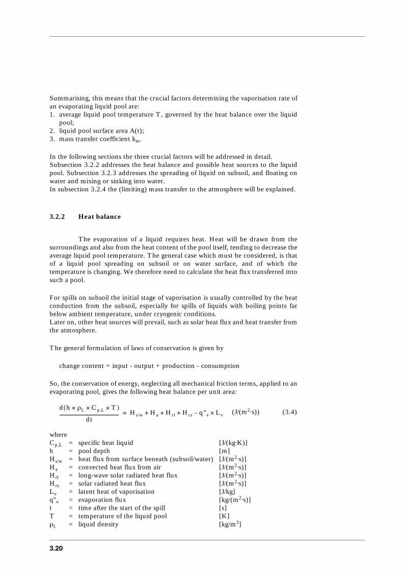
3.20
Summarising, this means that the crucial factors determining the vaporisation rate ofan evaporating liquid pool are:1. average liquid pool temperature T, governed by the heat balance over the liquid
pool;2. liquid pool surface area A(t);3. mass transfer coefficient km.
In the following sections the three crucial factors will be addressed in detail.Subsection 3.2.2 addresses the heat balance and possible heat sources to the liquidpool. Subsection 3.2.3 addresses the spreading of liquid on subsoil, and floating onwater and mixing or sinking into water.In subsection 3.2.4 the (limiting) mass transfer to the atmosphere will be explained.
3.2.2 Heat balance
The evaporation of a liquid requires heat. Heat will be drawn from thesurroundings and also from the heat content of the pool itself, tending to decrease theaverage liquid pool temperature. The general case which must be considered, is thatof a liquid pool spreading on subsoil or on water surface, and of which thetemperature is changing. We therefore need to calculate the heat flux transferred intosuch a pool.
For spills on subsoil the initial stage of vaporisation is usually controlled by the heatconduction from the subsoil, especially for spills of liquids with boiling points farbelow ambient temperature, under cryogenic conditions.Later on, other heat sources will prevail, such as solar heat flux and heat transfer fromthe atmosphere.
The general formulation of laws of conservation is given by
change content = input - output + production - consumption
So, the conservation of energy, neglecting all mechanical friction terms, applied to anevaporating pool, gives the following heat balance per unit area:
whereCp,L = specific heat liquid [J/(kg⋅K)]h = pool depth [m]Hs/w = heat flux from surface beneath (subsoil/water) [J/(m2⋅s)]Ha = convected heat flux from air [J/(m2⋅s)]Hrl = long-wave solar radiated heat flux [J/(m2⋅s)]Hrs = solar radiated heat flux [J/(m2⋅s)]Lv = latent heat of vaporisation [J/kg]q"v = evaporation flux [kg/(m2⋅s)]t = time after the start of the spill [s]T = temperature of the liquid pool [K]ρL = liquid density [kg/m3]
d h ρL× Cp ,L T××( )
dt------------------------------------------------ Hs/w Ha Hrl Hrs q"v Lv×–+ + += (3.4)(J/(m2⋅s))
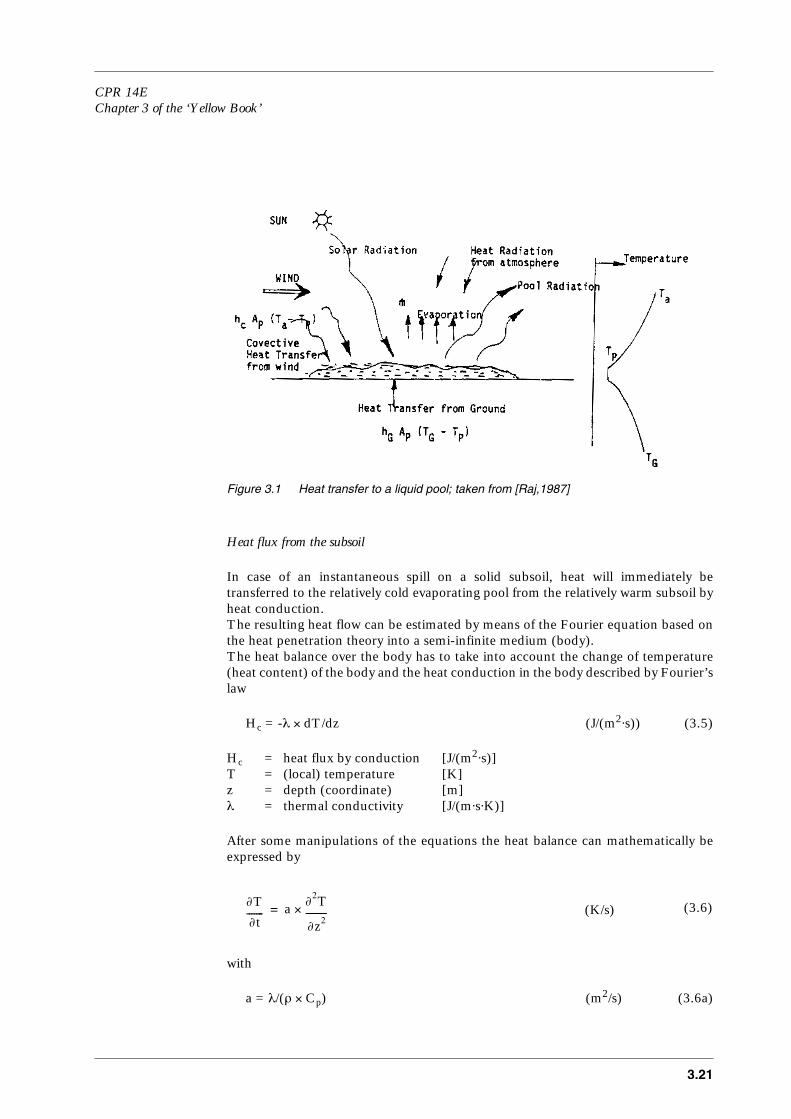
CPR 14EChapter 3 of the ‘Yellow Book’
3.21
Figure 3.1 Heat transfer to a liquid pool; taken from [Raj,1987]
Heat flux from the subsoil
In case of an instantaneous spill on a solid subsoil, heat will immediately betransferred to the relatively cold evaporating pool from the relatively warm subsoil byheat conduction.The resulting heat flow can be estimated by means of the Fourier equation based onthe heat penetration theory into a semi-infinite medium (body).The heat balance over the body has to take into account the change of temperature(heat content) of the body and the heat conduction in the body described by Fourier’slaw
Hc = -λ × dT/dz (J/(m2⋅s)) (3.5)
Hc = heat flux by conduction [J/(m2⋅s)]T = (local) temperature [K]z = depth (coordinate) [m]λ = thermal conductivity [J/(m⋅s⋅K)]
After some manipulations of the equations the heat balance can mathematically beexpressed by
with
a = λ/(ρ × Cp) (m2/s) (3.6a)
∂T
∂t------- a ∂2T
∂z2---------×= (3.6)(K/s)

3.22
wherea = thermal diffusivity [m2/s]Cp = specific heat [J/(kg⋅K)]
Assuming the following conditions: a. the body is initially at uniform temperature T0;b. resulting from a sudden fixed change in temperature at the outside to temperature
T1;c. due to the fact that the heat conducting medium is considered semi-infinite, the
temperature will not change at a very long (infinite) distance from the outside;
summarised mathematically:
a) initial condition: T(z,t) = T0 for z ≥ 0 at t = 0b) boundary condition: T(z,t) = T1 at z = 0 for t ≥ 0c) boundary condition: T(z,t) = T0 at z → ∞ for t > 0
whereT0 = initial temperature [K]T1 = new temperature [K]
By doing this the actual dimensions of finite heat conducting bodies are neglected,which leads to the remarkably simple analytical solution given by Fourier.Applied to the problem at hand this results in the time-dependent heat flux Hc(t)from the subsoil into the evaporating pool, and is given by
The total amount of heat conducted into the pool per square meter during the perioduntil time t, is given by
Q''H = 2 × Hc(t) × t (J/m2) (3.7a)
The denominator of the quotient , with dimension length, is often called‘heat penetration depth’, see Figure 3.2,
zp,H = (m) (3.8)
This penetration depth plays a roll in case the heat source can not be regarded assemi-infinite. In general the heat penetration theory may be applied if
zp,H = << rbody (m) (3.8a)
or
Fo < 0.2 (-) (3.8b)
with
Fo = a × t/rbody2 (-) (3.8c)
Hc t( ) λ– dT/dt z 0=×
λ T0 T1–( )×
a π t××( )-------------------------------= = (3.7)(J/(m2⋅s))
a π t××( )
a π t××( )
a π t××( )
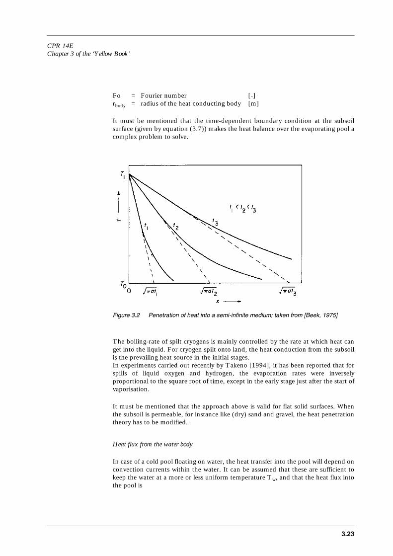
CPR 14EChapter 3 of the ‘Yellow Book’
3.23
Fo = Fourier number [-]rbody = radius of the heat conducting body [m]
It must be mentioned that the time-dependent boundary condition at the subsoilsurface (given by equation (3.7)) makes the heat balance over the evaporating pool acomplex problem to solve.
Figure 3.2 Penetration of heat into a semi-infinite medium; taken from [Beek, 1975]
The boiling-rate of spilt cryogens is mainly controlled by the rate at which heat canget into the liquid. For cryogen spilt onto land, the heat conduction from the subsoilis the prevailing heat source in the initial stages.In experiments carried out recently by Takeno [1994], it has been reported that forspills of liquid oxygen and hydrogen, the evaporation rates were inverselyproportional to the square root of time, except in the early stage just after the start ofvaporisation.
It must be mentioned that the approach above is valid for flat solid surfaces. Whenthe subsoil is permeable, for instance like (dry) sand and gravel, the heat penetrationtheory has to be modified.
Heat flux from the water body
In case of a cold pool floating on water, the heat transfer into the pool will depend onconvection currents within the water. It can be assumed that these are sufficient tokeep the water at a more or less uniform temperature Tw, and that the heat flux intothe pool is
3.24
Hw = kH,w × (Tw - T) (J/(m2⋅s)) (3.9)
where Hw = heat flux by heat transfer from water [J/(m2⋅s)]kH,w = heat transfer coefficient on water [J/(m2⋅s⋅K)]T = liquid pool temperature [K]Tw = water temperature [K]
For boiling on water surface three boiling regimes can be distinguished: nucleateboiling, transition boiling and film-boiling. The vapour bubble formation at the water liquid interfacing disturbs the heattransfer. The coalescence of bubbles may form an insulation layer between liquid andwater, leading to a decrease of heat transfer between water and liquid that results ina decrease of evaporation rate. This type of boiling is called metastable boiling. The heat transfer coefficient is different for each boiling regime.
If ice formation occured, this would have a considerable effect on the heat transferfrom the water body to the liquid pool.In the past ice formation was considered possible for releases of cryogens on still watersurfaces. The underlying references stem from 1975-1978. What is meant by the term‘still waters’ in this model remains unclear; for instance, it is unlikely that the depthof the water body would not be relevant.Zumsteg [1991] reports the formation of small ice particles under experimentalconditions, that were dragged by the evolving vapour due to a spill of cryogen ontowater. Chang [1982] also reported ice formation on the water surface in experimentson laboratory scale. A survey of experimental spills of cryogenic liquids is given inPrince [1985]; it appears that each cryogen behaves in its own typical way if spilt ontowater.However, there is experimental evidence that ice does not form at the water-cryogeninterface because of vigorous boiling. Water droplets may be carried into the evolvingvapour, [Melhelm, 1993]. Pool evaporation may be influenced by waves leading to a larger contact surface, andbetter mixing of the top layer of the water body. Webber assumes [Webber, 1990], that an ice crust will not be formed if cryogens arespilt on water. His model is intended for analyses of spills on large extents of waterand all evidence of ice formation seems to stem from small-scale experiments wherea limited amount of water was available as a heat source.
Heat flux from the atmosphere
The convected heat flux from air (Ha) is given by:
Ha = kH,a × (Ta - T) (J/(m2⋅s)) (3.10a)
wherekH,a = heat transfer coefficient to the atmosphere [J/(m2⋅s⋅K)]Ta = ambient temperature [K]

CPR 14EChapter 3 of the ‘Yellow Book’
3.25
The heat transfer coefficient kH,a may be estimated by assuming a turbulent flow overa flat plate by the following equations
Nu = 0.037 × Pra1/3 × Re0.8 (-) (3.10b)
for turbulent flow Re > 5 × 10⁵,
with
Nu = kH,a × (2 × rp)/λa (-) (3.10c)
Re = ρa × uw,10 × (2 × rp)/ηa (-) (3.10d)
Pra = υa/Da (-) (3.10e)
≈ 0.786
whererp = pool radius [m]Nu = Nusselt’s number [-]Pra = Prandtl’s number for air [-]Re = Reynolds’ number [-]uw,10 = wind speed at 10 metres height [m/s]ηa = dynamic viscosity air [N⋅s/m2]λa = thermal conductivity of air [J/(K⋅m⋅s)]ρa = density air [kg/m3]υa = kinematic viscosity of air [m2/s]Da = diffusion coefficient of air [m2/s]
Heat flux from radiation
The rate of long-wave radiation heat exchange (Hrl) between the pool surface and thesurroundings and the solar radiation (Hrs) can be calculated by equations (4.36) and(4.37) of the chapter Vapour cloud dispersion (page 4.62).
Heat transfer in the bulk of the pool
Studer [1988] states that a rigorous way to describe the evaporation of a liquid poolrequires an incorporation of all heat and mass transfer components, without ignoringthe impact of the intra-pool heat transfer resistance. This latter assumption isconsidered to be a conservative one, and often made implicitly by assuming a uniformliquid pool temperature.A deep pool, resulting from a major chemical release, behaves as if it consisted of twoseparate elements: a thin surface layer and the bulk liquid pool.Studer shows the effect of intra-pool heat transfer resistance can be ignored in casethe initial height of the instantaneous pool is about 4 metres. It may be expected, however, that the bulk heat transfer resistance will have asubstantial effect on spills in bunds with huge barriers, but not in case of unboundedspreading while the liquid height quickly diminishes in time.

3.26
3.2.3 Pool spreading
Released liquid will spread onto the subsoil or the water surface in the immediatevicinity of the failing containment.The spreading will continue unless the pool is contained by a dike or channelled intoa sump, or when the liquid has spread to such an extent that its thickness is of thesame magnitude as the subsoil roughness, or until the evaporation rate is equal to therelease rate so that the amount of liquid in the pool does not increase any more. The maximum pool diameter of a spreading liquid pool will depend on thetopography of the subsoil near the release point. In industrial plants often vessels havebeen placed in bunds (low walls or dikes). In case the pool is confined to a bund thesurface area of the pool is limited. If not, the liquid pool will spread and the surfacearea of the pool will be a function of time during a large part of the evaporation.
On subsoil most liquid spills at industrial plants will be confined, however not in thecase of transportation. Spills onto water will be unbounded, although the width of thewater body (channels) may act as a barrier. In practice, very often no barrier isprovided around storage tanks for gases liquefied by compression. This means thatfor the determination of the evaporation of released condensed gases, the spreadingof the liquid must be considered. The extent of spreading of an unconfined liquid spillis a key factor that effects the emission rate from the pool surface. As the liquid spreads, three flow regimes are recognised [Melhelm, 1993]:1. gravity - inertia regime: gravitational acceleration of the descending liquid mass is
counter-balanced by inertia,2. gravity - viscous regime: in which the gravitational spreading force is opposed by
friction at the liquid-subsoil interface,3. surface tension - viscous regime: in which for very thin liquid films, surface tension
replaces gravity as the driving force.
Cryogenic spills rarely reach the gravity-inertia regime because of their rapidevaporation. The surface tension – viscous regime is of importance for heavyhydrocarbons on water.For the calculation of the evaporation of liquefied gases on subsoil, a distinctionshould be made between a permeable and a non-permeable subsoil, as the spilt liquidmay sink into the ground.
3.2.3.1 Release on land within bunds
The presence of second containments (bunds) reduces the evaporation rateby limiting the pool area, and providing for longer contact times between liquid andsubsoil, leading to reduction of heat conduction from the subsoil to the evaporatingliquid [World Bank, 1988].In case the liquid is caught in a bund, the spreading of the spill will be limited. Themaximum pool size will be the size of the bund. Of course, this will only be the casewhen the dimensions of the bund are well designed. If the bund is too small, thereleased liquid will simply spill over the dike. Furthermore, bund overtopping due todynamic force may be the cause for secondary containments not to be able to copewith a sudden release of large amounts of liquid [Wilkinson, 1991].

CPR 14EChapter 3 of the ‘Yellow Book’
3.27
Also in Phelps [1992] a model based on computational fluid dynamics has beenpresented that is able to predict the behaviour of a running liquid against vertical orinclined walls.
3.2.3.2 Continuous release on land without a bund
The pool will stop spreading when the release of liquid has stopped due toa cut-off or exhaustion. Also when the evaporation rate of the pool equals the releaserate on the subsoil the pool will reach its maximum diameter.In case of a continuous release of liquid, the liquid pool will eventually reach a specificdepth, where evaporation through the surface balances the steady discharge into thecentre of the pool.
A simple model of viscous effects appears reasonably realistic [Webber, Apr. 1991]and leads to depth of order
whereg = acceleration due to gravity [m/s2]hc,∞ = minimum depth spreading and vaporising [m] liquid pool under a steady dischargeqS = liquid source discharge rate [kg/s]υL = kinematic liquid viscosity [m2/s]ρL = liquid density [kg/m3]
Experimentally, Moorhouse and Carpenter [Webber, Apr. 1991] have studiedcontinuous releases of LNG on smooth concrete, and concluded a spreading depthof around 1 centimetre.
3.2.3.3 Instantaneous release on land without a bund
In practical situations the pool will spread until it reaches some minimumthickness which is related to the surface roughness. As typical values a lower limit of5 millimetres for very smooth surfaces and for rough surfaces several centimetres weresuggested earlier, see table 3.1.Another suggestion is simply to assume a maximum pool area based on thetopography of the surroundings, according to the analyst’s judgement.
hc ,∞
6 υL qS××
ρL π g××( )---------------------------
0.25
= (3.11)(m)

3.28
Table 3.1 Characteristic average roughnesses of some subsoils
The pool area can be estimated conservatively by assuming that all of the releasedliquid spreads instantaneously to the minimum thickness, and reaches its maximumpool size immediately.This simplifying assumption leads to overpredictions for the vaporisation rate shortlyafter the spill. This can be neglected for non-boiling volatile liquids because of therelatively long duration of the evaporation at low evaporation flux q"v.
Low volatile liquid releases at ambient conditions evaporate at considerable rates onlywhen the pool surface is relatively large, compensating for a relatively lowvaporisation mass flux. This may be the case when large amounts of liquid run into alarge bund or can spread out to a large extent.
3.2.3.4 Evaporation of chemicals mixed in water [Raj, 1974]
When a soluble chemical water is spilt on water, it rapidly dissolves.Chemicals may not only be readily miscible with water, but may also have highvapour pressures at ambient temperature. When such liquids are spilt, vapour may begenerated. When a water-miscible liquid is spilt on a water surface, mixing takesplace, thereby diluting the spilt liquid. The mixing is caused by molecular diffusion in calm water and mass convection(turbulent diffusion) in streaming rivers. In rivers, the main cause for mixing is streamturbulence. Mixing may take place preferentially in one direction. It depends on flowconditions, flow geometry and water density gradients.In rivers, waves are not important. In general the effects of salinity-driven mixing canbe ignored.
3.2.3.5 Evaporation of chemicals that sink in water [Raj, 1974]
There are many liquid chemicals with densities larger than that of water,whose boiling point at atmospheric pressures are less than the water temperature, forinstance, chlorine. When such liquids are spilt on water, they may sink and vaporiseat the same time because of their low-boiling point. When a large mass (‘blob’) of a heavy liquid is spilt on the surface of water in a veryshort time, the liquid sinks ‘en masse’ only for a small depth. The increasing sinkingvelocity of the blob results in a pressure force on the front face. When this pressureforce exceeds the internal resistance of the blob, the blob will be broken into small-
Subsoil Average roughness(m)
Flat sandy soil, concrete, stones, industrial site 0.005Normal sandy soil, gravel, railroad yard 0.010Rough sandy soil, farmland, grassland 0.020Very rough, grown over sandy soil with pot-holes 0.025

CPR 14EChapter 3 of the ‘Yellow Book’
3.29
sized drops. Due to the break-up of the large blob of heavy liquid into smaller drops,the liquid will evaporate rapidly due to massive heat transfer from the surroundingwater.
Figure 3.3 Schematic illustration of the sequence of blob break-up into drops [Raj, 1974]
The parameter which determines the stability of a blob or a drop, or resistance tobreaking, is the Weber number, being the ratio of the pressure force to the surfacetension force:
We = ρw × ud,∞2 × rd/σ (-) (3.12)
We = Weber number [-]ρw = density water [kg/m3]ud,∞ = terminal velocity of deformable drops [m/s]rd = drop radius [m]σ = liquid surface tension [N/m]
Experimental evidence indicates that most liquids tend to break-up when the Webernumber is larger than about 10. It can be shown that the duration over which a largemass, such as occurs in a spill, breaks up into smaller drops, is very short.Experiments indicate that, when a big blob breaks up, drops of various sizes areformed with the drop-size distribution being a function of various physical properties,parameters such as the properties of the liquid and the medium, the agency whichcauses the break-up, and others.
3.30
3.2.4 Mass transfer
For liquids having normal boiling points near or above ambienttemperature, mass transfer by diffusion will be the limiting factor. The wind isremoving vapour from the pool surface, and due to the resulting concentrationgradient mass transfer is induced; liquid will evaporate in order to restore the partialpressure which is in thermodynamic equilibrium to the liquid in the pool at itstemperature.So, the evaporation of a non-boiling liquid depends mainly on the rate at which thevapour can be removed by the air flow above the pool. In case of boiling liquids with a mass transfer that is very fast, the mass transferresistance may be neglected as a reasonable first approximation.
When a volatile (non-boiling) soluble liquid is spilt into water, the vaporisation of thechemical takes place only at the water surface, and is caused by the difference in(partial) vapour pressure of the solved chemical at the water surface and in theatmosphere. The evaporation mass flux q"v depends on the mass transfer coefficient(km) and the vapour concentration (ci) at the liquid pool surface. The vapourconcentration is proportional with the saturated vapour pressure of the liquid at thepool surface, depending on its temperature. Applying the ideal gas law results to
q"v = Dv × dci/dz
= km × ci(z = 0)
≈ km × Pv(Tps) × µi/(R × Tps) (kg/(m2⋅s)) (3.13)
whereci = concentration component i [kg/m3]Dv = diffusion coefficient vapour in air [m2/s]km = mass transfer coefficient related to concentration [m/s]q"v = vaporisation mass flux [kg/(m2⋅s)]Pv(T) = vapour pressure at temperature T [N/m2]R = international gas constant [J/(mol⋅K)]Tps = liquid temperature at pool surface [K]z = coordinate in vertical direction [m]µi = molecular weight of substance i [kg/mol]
Several empirical correlations for estimation of the mass transfer coefficient have beenproposed in literature in the following generalised form
km = f (uw,10, rp, Sc) (m/s) (3.14)
with
Sc = υV/Dv (-) (3.14a)
whererp = liquid pool radius [m]Sc = Schmidt number [-]Dv = diffusion coefficient of vapour into air [m2/s]

CPR 14EChapter 3 of the ‘Yellow Book’
3.31
υV = kinematic viscosity vapour [m2/s]uw,10 = wind speed at standard 10 metres height [m/s]
A model for the mass transfer coefficient km based on a more up-to-dateunderstanding of the turbulent atmospheric flow has been developed by [Brighton,1987]. In this model molecular diffusion is incorporated in the boundary conditions.
Experimental data about mass transfer from evaporating liquid pools as reported inKawamura and MacKay [1987] are given below. Note that the wind velocity was notmade explicit in this publication.Note that the dimensions of the air temperature and vaporisation mass flux aredegrees Celsius ˚C and kg/(m2⋅h) respectively.
Table 3.2 Steady state evaporation rate of liquid pools (after 15 minutes), without subsoil conduction (insulated pan)
Chemical Tair(˚C)
q"v(kg/(m2⋅h))
1 Toluene 21 4.49 2 Toluene 29 3.39 3 Cyclohexane 24 5.89 4 Cyclohexane 25 5.89 5 Hexane -5 5.55 6 Hexane 22 10.88 7 Methanol 7 2.55
8 Dichloromethane -6 9.49 9 Dichloromethane 1 7.5310 Dichloromethane 21 16.2711 Dichloromethane 25 17.9812 Pentane 1 10.5213 Pentane 5 6.8414 Pentane 7 8.1315 Pentane 9 10.4116 Freon11 0 33.0117 Freon11 17 34.93

3.32
Table 3.3 Average evaporation rate of liquid pools during the experiment, with subsoil conduction.
Note that in conformity with the original publication the vaporisation mass flux has been given in kilogram per square metre per hour, and the temperature in degrees Celsius.
Chemical Tair(˚C)
q"v(kg/m2⋅h)
18 Toluene 25 3.9019 Cyclohexane 29 9.3820 Hexane 27 7.2821 Pentane 23 23.0022 Pentane 25 27.1023 Freon11 31 34.88
CPR 14EChapter 3 of the ‘Yellow Book’
3.33
3.3 General overview of existing models
3.3.1 Introduction to section 3.3
The various models for pool evaporation on subsoil or water surfacepresented in the open literature have a broadly similar structure [Webber, 1991].All models comprise a heat balance, pool spreading models, and correlations for thelocal vaporisation flux.The models differ in:– the number of heat sources taken into account;– the collection of selected submodels for spreading and mass transfer;– the way of approximation by analytical solutions (partially);– the degree of complexity due to ignoring effects;– the applied numerical methods to solve the set of equations.Most models have been based on the same limited number of publications dealingwith mass transfer to the atmosphere and pool spreading.
In general the classic models are based on the sharp distinction between boiling andnon-boiling liquids, on a non-adequate representation of the expected behaviour ofpools of different viscosity on different surfaces [Webber, 1991], and sometimes stillon the rather antique mass transfer relation of Sutton. Furthermore, simplifyingassumptions were made to describe the spreading of the pool. These models can be improved from a scientific viewpoint and from the viewpoint ofan adequate numerical solution. Advanced and complete but complex models havebeen found in recent literature. The pool evaporation model GASP has beendeveloped by SRD(AEA)/HSE. Similar models have been found in literature.
In the following section, submodels will be addressed first, dealing separately with theheat balance, mass transfer, or pool spreading.In this section the following themes are addressed:– subsection 3.3.2 addresses the submodelling of the heat balance;– subsection 3.3.3 addresses the submodelling of pool spreading;– subsection 3.3.4 addresses the submodelling of mass transfer;– subsection 3.3.5 addresses recent models, which solve the problem integrally.
3.3.2 Heat balance
Simple modelling is based on a sharp distinction between boiling and non-boiling liquids. A sudden switch between models have to be made when describingthe transition from boiling to non-boiling. This results in a rather unpleasantdiscontinuity in the evaporation rate at an arbitrary vapour pressure.In the modelling of evaporation of boiling liquids, only the heat conduction from thesubsoil or from the water surface has been taken into account.
In recent models [Webber, 1990], [Woodward, 1990], [SuperChems 4.0] thecomplete heat balance is taken into account and thus none of the heat sources areignored to simplify the model; see paragraph 3.2.2. No principal distinction is madebetween boiling and non-boiling pools.
3.34
3.3.2.1 Film and nucleate boiling on water surfaces
In the previous YellowBook a method has been described to estimate theboiling rate of a cryogen on a water surface, which has been recognised as meta-stableboiling for most industrial commodities [YellowBook, 1988].
In the GASP-model a more simplified approach has been chosen. It is assumed thatthe spilt chemical boils in the film-boiling regime when the heat flux into the liquidpool exceeds the so-called critical heat flux. If not, the heat flux into the pool isdescribed with a constant heat transfer coefficient.
3.3.3 Pool spreading
3.3.3.1 Pool spreading on land
Simple models for pool spreading on solid surface
Simple spreading models consist of simple mathematical expressions, mostly powerexpressions, that relate the radius of the spreading liquid pool to the time from thestart of the release
r(t) = Cs × tEs (m) (3.15)
r = radius of the spreading liquid pool [m]t = time from of the release [s]
The values for constant Cs and exponent Es differ for liquids spreading on land andfor liquids spreading on water. The constant Cs and exponent Es depend on the typeof release: continuous or instantaneous.An overview of these simple models can be found in Raj [1981], Raj [1987]. Othermodels have been given in Shaw [1978], WorldBank [1988], Melhelm [1993] andFrie [1992]. Most remarkable is that the model equations of the three groups differ, regardingwhich seem qualitatively the same spreading conditions.
Obviously, this varied collection of relations leads to the conclusion that correlationshave been made for different situations or have been based on different assumptions.Many previous analyses based on ordinary differential equations, have used thesimple assumption that the radial spreading rate (u) of a circular liquid pool isproportional to , where (g) is the acceleration due to gravity and (h) is themean pool depth. For pools spreading on water, this is valid for a restricted timeinterval after any initial radial acceleration phase and before the pool becomes thinenough for turbulent or viscous effects to become important. In this case (g) must bemultiplied by the relative density difference. In other circumstances the spreadingbehaviour is quite different and generally more complicated [Webber, Jan. 1991].
g h⋅( )
CPR 14EChapter 3 of the ‘Yellow Book’
3.35
The sharp distinctions between instantaneous and continuous releases, and betweenspreading liquid pools and fixed (confined) pools, are made to simplify the spreadingmodel. These rather academic idealisations always shift the problem to theapplication of the model in practical situations. Consequently, often these idealassumptions will not hold.
Shallow layer equations governing pool spreading on land
It should be noted that the sharp distinction between continuous and instantaneousreleases, which is basically made in the simple spreading models, puts forward thequestion what to choose in case of semi-continuous or time-dependent releases thatappear in reality. In the following a more general approach is made in order to coverthe whole range of different spreading regimes for different types of liquid releases.
If the horizontal dimension of the pool is much larger than its depth, the usual fluidequations may be reduced to the approximate form, the so-called ‘shallow layerequations’, [Webber, 1986]. In case of axial symmetry and instantaneous release,ignoring the vaporisation, the horizontal momentum equation may be expressed as
∂u/∂t + u × ∂u/∂r = -g × ∂h/∂r (m/s2) (3.16)
and secondly, the conservation of mass:
∂h/∂t + u × ∂h/∂r + h/r × ∂(r × u)/∂r = 0 (m/s) (3.17)
whereu = radial velocity [m/s]r = radius of the spreading liquid pool [m]h = liquid pool height [m]g = gravitational acceleration [m/s2]
Instead of the gravitational acceleration on subsoil, the reduced acceleration due togravity will be needed for pools spreading on water.The process of pool spreading is controlled by the gravitational acceleration of thedescending liquid mass and the surface tension, versus the inertia of the liquid massand the friction due to liquid viscosity.
The solutions that can be derived for the shallow layer equations will not be in theform of one simple power relation for the growth of the pool radius versus time:r(t) ≈ tn. However, the solution may be somewhat artificially split up into regimes.These regimes could be approximated by power relations r(t) ≈ tn, although these aremerely a tangent to the curve, [Webber and Brighton, 1987].For pools spreading on subsoil, the following approximating power relations could bedistinguished:
1a. inviscid or gravity-inertia regime: r(t) ≈ (m) (3.18a)
1b. gravity-turbulent regime: r(t) ≈ C2 × t2/7 (m) (3.18b)
2. gravity-viscous regime: r(t) ≈ C3 × t1/8 (m) (3.18c)
C0 C1 t2×+( )

3.36
Figure 3.4 A non-volatile pool spreading on subsoil; [Webber and Brighton 1987]
For spills onto water the density difference between water and the floating liquidshould be taken into account, and, furthermore, the motion of the water beneath thepool [Webber and Brighton, 1987]:
1a. inviscid or gravity-inertia regime: r(t) ≈ C4 × t1/2 (m) (3.19a)
1b. gravity-turbulent regime: r(t) ≈ C2 × t2/7 (m) (3.19b)
2. gravity-viscous regime: r(t) ≈ C5 × t1/4 (m) (3.19c)
Obviously one simple power relation between pool radius versus time can notdescribe the spreading of a pool on a flat surface for all regimes. This may explain whyso many spreading relations have been found in literature.
Evaporation of cryogen (boiling liquid) on a permeable subsoil
A spilt cryogen may soak into permeable subsoil. Freezing of water in the soil columnmay prevent the liquid from penetration into the subsoil. Obviously, the effect of percolation into the subsoil is more important for small spillsthan large spills where the liquid pool may be substantially thicker than thepenetration depth into the subsoil.
Models for evaporation of cryogens have been given earlier for dry and moist poroussubsoil and gravel layers [YellowBook, 1988]. These models are all based on thetime-dependent heat penetration theory as has been explained in paragraph 3.2.2.
In Takeno [1994], laboratory experiments have been reported in which cryogenicspills of oxygen on a dry sand layer, liquid oxygen was observed to vaporise while
CPR 14EChapter 3 of the ‘Yellow Book’
3.37
constantly soaking into and rolling up the upper section of the layer. The leading edgeof the rolled-up sand layer was observed to move downwards into the sand layer.
The evaporation rate was determined simply by the velocity of liquid penetration intothe dry sand layer, which was nearly independent of the liquid depth. This indicatesthat the evaporation rate is independent of time and that its rate can be determinedby the liquid penetration velocity alone, by
H = ρss × Cp,ss × (Tss,0 - Tb) × (1 - εp) × up (J/(m2⋅s)) (3.20)
H = heat flux [J/(m2⋅s)]ρss = density of sand [kg/m3]Cp,ss = specific heat of sand [J/(kg⋅K)]Tss,0 = initial sand temperature [K]Tb = boiling point liquid [K]εp = porosity (void fraction) sand [-]up = penetration velocity in the sand [m/s]
In the experiments the liquid penetration velocity was merely constant at about0.0014 m/s, regardless of the liquid depth. Unfortunately, Takeno [1994] does not supply a model for the calculation of thepenetration velocity in the sand up, and an additional submodel have to be taken fromelsewhere.
The penetration of fluids into soil is a complex phenomen which depends on the type,geometry and resistance properties of the soil, the penetrating material properties andambient conditions [Melhelm, 1992].The penetrating fluids into soil is governed by gravitational and capillary forces. Incase of low-boiling fluids and cryogens the evolving vapour will cause an oppositevapour flow against the soaking liquid. Apparently the upward force due to the out-blowing vapour due to vaporisation by extracting heat from the sand grains, is inequilibrium with gravitation. When the heat content of the sand at a certain height isexhausted, the liquid will sink deeper into the subsoil.A rather simplified model presented in Melhelm [1992] assumes liquid penetrationto behave as saturated piston flow, influenced by gravitational forces only. So, in thisapproach all effects of capillary forces, vaporisation of liquid, freezing of the moisturein the subsoil, lateral spreading and heat conduction, have been neglected. InMelhelm [1992] the penetration depth of liquid soaking into porous subsoil is givenby
zp = K0 × tz (m) (3.21a)
K0 = ρL × g × asi/ηL(Tb) (m/s) (3.21b)

3.38
So, that
up ≈ K0 (m/s) (3.21c)
whereasi = intrinsic permeability of the soil [m2]g = gravitational acceleration [m/s2]K0 = hydraulic conductivity of the soil [m/s] at saturated conditionstz = time of penetration [s]ρL(Tb) = liquid density at boiling point [kg/m3]zp = depth of liquid penetration [m]ηL(Tb) = dynamic viscosity liquid at boiling point [N⋅s/m2]
Some values for the intrinsic permeability have been given in Melhelm [1992].
Table 3.4 Intrinsic permeability for some subsoil types
The remarkably different outcome of both models in Yellow Book [1988] andTakeno [1994] concerning the time-dependency of the evaporation rate, might bedue to a difference in ratio between the initial liquid height and the height of the sandlayer.
3.3.3.2 Releases of non-floating chemicals on water
Mixers
HACS-R is an evaporation model for volatile water-soluble chemicals into water, likemethanol. It has been developed for U.S. Coast Guard by Raj and is described in aNTIS-report [Raj, 1974]. Dodge reported good model performance in 1982.It is assumed that the entire liquid spilt goes into solution in water first. Afterestimating the liquid concentration in the water, the vapour pressure on the watersurface of the chemical can be estimated, as well as the vaporisation rate. The model HACS-R has recently been applied with some modifications[Dharmavaram, 1994].
Subsoil type asi(m2)
coarse sand 10-9
silty sand 10-12
clay till 10-15

CPR 14EChapter 3 of the ‘Yellow Book’
3.39
Sinkers
In a NTIS-report [Raj, 1974] a model has been given describing the evaporationphenomena for liquids heavier than water with boiling temperatures less thanambient.An evaporative model has been worked out based on the assumption of dropformation when a blob of heavy, low-boiling-point liquid is spilt on a water surface.It has been assumed that the initial blob of liquid breaks up into uniform and equally-sized drops because of pressure forces and instability of the blob.The details of drag on a deformable drop have been included in the analysis tocalculate the terminal velocity of drops. A heat-mass similarity model is used topredict the vaporisation rate. In this model it is assumed that the liquid is immisciblewith water.
3.3.4 Mass transfer
The wind is removing vapour from the pool surface, and due to theresulting concentration gradient, mass transfer is induced; liquid will evaporate inorder to restore the partial pressure which is in thermodynamic equilibrium to theliquid in the pool at its temperature. Thus, the evaporation of a non-boiling liquiddepends mainly on the rate at which the vapour can be removed by the air flow abovethe pool.
The evaporation mass flux q"v depends on the mass transfer coefficient (km) and thevapour concentration ci at the liquid pool surface
q"v = km × ci(z = 0) (kg/(m2⋅s)) (3.2)
whereci = concentration component i [kg/m3]km = mass transfer coefficient [m/s]q"v = vaporisation mass flux [kg/(m2⋅s)]z = coordinate in vertical direction [m]
The dimensionless correlation of Raj & Morris for the mass transfer coefficient km, isbased on the heat-mass analogy [Raj, 1987], [Studer, 1988]
Sh = 0.037 × (Re0.8 - 15500) × Sc1/3 (-) (3.22)
with
Sh = km × lp/Dv (-) (3.23a)

3.40
and
Re = ρa × uw,10 × (2 × rp)/ηa (-) (3.23b)
whereRe = Reynold’s number [-]ρa = density air [kg/m3]uw,10 = wind speed at standard 10 metres height [m/s]ηa = dynamic viscosity air [N⋅s/m2]Sh = Sherwood’s number [-]km = mass transfer coefficient [m/s]lp = length pool along-wind direction [m]Dv = diffusion coefficient vapour in air [m2/s]
Note that Sherwood’s number Sh for mass transfer is on the analogy of the Nusselt’snumber Nu for heat transfer.
In the past the correlation of Sutton has been given for the mass transfer coefficientkm. This relation works well for laboratory experiments but the peculiardimensionality of the result makes extrapolation suspect [Webber, 1987].
A similar model has been given by MacKay & Matsugu [Kawamura, 1987] which hasbeen validated against a number of experiments
km = Cm&m × uw,100.78 × (2 × rp)-0.11 × Sc-0.67 (m/s) (3.24)
with
Sc = υV/Da (-) (3.25)
whereCm&m = 0.004786 [m0.33/s0.22]Da = diffusion coefficient vapour in air [m2/s]km = mass transfer coefficient [m/s]rp = radius of the liquid pool [m]uw,10 = wind speed at standard 10 metres height [m/s]Sc = Schmidt number [-]υV = kinematic viscosity vapour [m2/s]
Note that in general for gases and vapours, Sc ≈ 0.8. The original relation of MacKay& Matsugu was expressed in other dimensions.The correlations by Sutton, Raj and Kawamura have the Schmidt number incommon. In Brighton [1990] it is stated that the exponent is under dispute and is nosound basis for up-scaling the results derived from laboratory experiments only.The alternative model of Brighton is based on scientific knowledge about atmosphericturbulence [Brighton, 1987]. In this model molecular diffusion is incorporated in theboundary conditions. The model is valid for neutral atmospheric stability. Brighton’stheory can be matched with experiments although deviation between predictions andexperimental results is large.
CPR 14EChapter 3 of the ‘Yellow Book’
3.41
3.3.5 Advanced integral models
3.3.5.1 GASP
Quite recently, SRD/HSE developed the model GASP. GASP is anacronym for ‘Gas Accumulation over Spreading Pools’ [Webber, 1990]. GASP is anevaporation model that has incorporated all of the heat and mass transfercomponents. GASP solves the set of equations based on a complete heat balance andthe shallow water equations (3.16) and (3.17) governing the pool spreading both onsubsoil or water surface simultaneously. The mass transfer model is based on thework of Brighton [Brighton, 1987]. The model forces the transition of boiling to non-boiling to be smooth.
The model is able to give correct predictions [Webber, 1990]. The GASP model isonly able to cope with (spreading) pools on a subsoil and onto water surface. It is notable to deal with volatile soluble liquids into water, and boiling liquids heavier thanwater that will sink. The GASP model, and the research and data which it is basedupon, have been extensively given attention by several SRD/HSE-publications. The numerical procedure to solve the equations seems to be robust and does not taketoo much time on a 486-PC. The computerised model is commercially available.
3.3.5.2 LPOOL
In Woodward [1990] the model LPOOL is given. The model has beendeveloped by Technica Inc. The model is a complete pool evaporation model.
The model makes use of a grid of annular rings to solve the two-dimensional shallowlayer equations for radial flow over flat terrain (3.16) and (3.17). It relies on the masstransfer coefficient of MacKay and Matsugu, [Kawamura and MacKay, 1987]. Theheat transfer coefficient on water has been correlated to the heat of evaporation (noreferences)
kH,w = CH × Lv (J/(m2⋅K⋅s)) (3.26)
with
CH = 0.001
wherekH,w = heat transfer coefficient [J/(m2⋅K⋅s)]Lv = heat of evaporation [J/kg]CH = correlation coefficient [kg/(s⋅m2⋅K)]
Also numerical methods have been briefly addressed regarding how to solve the set ofequations. The solutions of the set formed by the continuity equation (mass balance)and (momentum balance) and submodels are found by using a Crowley second-orderfinite difference solution, superimposing the homogeneous and forced solution.
3.42
The spreading model has been validated against small-scale, low-release-rateexperiments of Belore and McBean who tested pool spread rates with water, and datafor crude oil spilt onto frozen arctic ground.The model has been computerised and is commercially available, though part of amuch larger software package [Technica, 1994].
3.3.5.3 SuperChems
The large software package SuperChems of A.D. Little comprises a poolevaporation model that is based on a time-dependent solution of the ‘shallow waterequations’ [Superchems 4.0]. It calculates the liquid regression rate for a spreadingpool on different soil types and water. Solubility of the chemical spilt in water isincorporated. The complete heat balance accounts for all possible heat sources. Thedifferent spreading regimes are also accounted for. The model accepts time-dependent release rates. The model is commercially available.

CPR 14EChapter 3 of the ‘Yellow Book’
3.43
3.4 Selection of models
3.4.1 Introduction to section 3.4
In section 3.4 the considerations which have led to the selection of themodels that are included in section 3.5, will be explained. In section 3.5 these modelswill be described in detail. In general the selection is based on the following considerations:1. The availability of powerful (personal) computers creates the opportunity to avoid
simplified (analytical) solutions, that are only able to cope with idealisedsituations.
2. Models based on computational fluid dynamics (CFD) can not be used in safetystudies and hazard assessment, due to the time-consuming data collection in orderto supply the required input and analysis of the results, and due to the largecomputer power they require.
3. Models should have been validated against unambiguous experimental data.4. Increased complexity of the model must result in more reliable predictions;
unnecessary complications should be avoided.5. The model should be available in literature; and preferably available in
computerised form at minimum cost
3.4.2 Pool evaporation on subsoil and on water surface
In addition the selection of liquid pool evaporation models has been basedon the following considerations:1. The heat balance should take into account all heat source terms;2. The artificial distinction between boiling and non-boiling liquids should be
avoided;3. The spreading of the liquids should be described by solutions of the shallow layer
equations, giving a general solution;4. The mass transfer should be modelled by a widely applicable model based on
experimental data.
Advanced and complete models have been found in recent literature.The pool evaporation model GASP has been developed by SRD(AEA)/HSE.Similar models have been found in literature: LPOOL [Woodward, 1990],SuperChems of A.D. Little [Superchems 4.0].The recent integral models are really a step forward in supplying a realistic descriptionof the pool evaporation. A major drawback is the relatively high cost of computerisedversions commercially available.Based on the accessibility of the model description in literature, and availability of thecomputer program, it was preferred to describe the GASP model in more detail in thefollowing section.The mass transfer model developed by Brighton [Brighton, 1987] is underdevelopment and has limited applicability. For practical situations it would beadvisable to use the correlation of MacKay and Matsuga, [Kawamura and MacKay,1987], because it is based on experiments carried out in the open. However, theGASP model uses Brighton’s model. For reasons of consistency, the description ofthe GASP model follows the original publications.

3.44
The GASP model is not able to predict evaporation rates of volatile soluble liquids inwater. However, the HACS-R model [Raj, 1974] is.
3.4.2.1 Boiling regimes
In literature a lot of attention is given to nucleate boiling and film-boiling.However, metastable boiling is often not taken into consideration, due to itscomplexity. Many common industrial liquefied gases will boil in the metastable boiling regime.So, the evaporation should be based on the model for metastable boiling. It must bementioned however that the selected GASP-model applies a somewhat simplifiedapproach to incorporate the effects of film-boiling.
3.4.2.2 Evaporation of cryogen on sand
Two remarkable different models have been encountered regarding theevaporation of cryogenes on sand.The approach by Takeno [1994] looks promising, but an adequate model to calculatethe penetration velocity of the boiling liquid into the subsoil is lacking and can noteasily be developed. Nevertheless, the extended model of Takeno has been addressedin detail in paragraph 3.3.3.1.While the model for liquid penetration is probably too simple, the TNO-model forevaporation on sand is to be preferred. It must be mentioned however, that the modelin YellowBook [1988] concerning evaporation in gravel layers ignores all kind ofcomplications, and may give unrealistically high evaporation rates. Therefore, someadditional criteria have to be added.
3.4.3 Evaporation of chemicals mixed in water
In the NTIS-report [Raj, 1974] a model has been given that describs theevaporation phenomena for volatile liquids which are soluble or miscible in water andhave a boiling point greater than the water temperature, but less than 100 ˚C. So, thechemical must have a considerable vapour pressure at water temperature. Because itis the only model found in literature to predict evaporation rates the HACS-R modelwill be described. In the literature it is reported that the HACS-R model has recently been used forprediction of the evaporation rate of an ammonia spill onto water [Dharmavaram,1994].
3.4.4 Evaporation of chemicals that sink in water
In the NTIS-report [Raj, 1974] a model has been given that describes theevaporation phenomena for liquids heavier than water with boiling temperatures lessthan ambient. The use of packed-bed correlation or single-sphere heat transfer

CPR 14EChapter 3 of the ‘Yellow Book’
3.45
correlations in the model leads to high evaporation rates. In general all of the spiltliquid is predicted to vaporise within a period of about 10 seconds. No experimental evidence is available to test the results of this theory. For dispersion predictions purposes, it is acceptable in most cases just to assume ainstantaneous release in case of a spill of a boiling liquid heavier than water. It maybe valid to use the spill rate itself as the evaporation rate in the case of semi-continuous spills. Therefore the model will not be included in section 3.5.
3.4.5 Application of simple models
The GASP-model is a very complex model and has to be computerisedbefore any prediction can be made.In case spreading of the liquid pool can be ignored, as may be the case forinstantaneous liquid releases in bunds, it is possible to use simple models to guess themagnitude of the evaporation rate, at least with some accuracy.So, for convenience, simple models will also be presented in section 3.5, though theGASP model is to be preferred from a scientific point of view.

3.46

CPR 14EChapter 3 of the ‘Yellow Book’
3.47
3.5 Description of models
3.5.1 Introduction to section 3.5
Section 3.5 provides descriptions of the recommended models andmethods for liquid pool evaporation. It contains all necessary information to performthe calculations. For background of the models the reader should review section 3.3.
Section 3.5 provides detailed descriptions of the models and methods regarding thefollowing topics. Subsection 3.5.2 gives a description of GASP valid for liquid pools(spreading) on subsoil and floating on water. Subsection 3.5.3 and 3.5.4 treat the evaporation of cryogenes on subsoil and water.Subsection 3.5.5 provides simple models for pool evaporation in bunds, for whichcomplicated calculations may be avoided without losing too much accuracy.Subsection 3.5.6 gives a description of HACS-R, valid for volatile (non-boiling)liquid chemicals into water. In section 3.8 some additional remarks on the limitations of the models presented aregiven.
3.5.2 GASP [Webber, 1990]
3.5.2.1 Introduction
GASP is an acronym for ‘Gas Accumulation over Spreading Pools’. Thedescription of the GASP model has been taken from ‘A model for pool spreading andvaporisation and its implementation in the computer code G*A*S*P’, by D.M.Webber [Webber, 1990]; courtesy AEA-technology.
The GASP model aims at the description of the spreading and vaporisation of aevaporating liquid pool to predict the evaporation rate and pool size.
The complete specification of the model will be concise and will use results that havebeen derived by others. References made in the original publication of Webber[Webber, 1990] will not be repeated here.The model will be defined with reference to the computational methods which areused to solve the equations, and relevant numerical aspects will be touched uponhere.
The model is able to predict the vaporisation rate of a circular liquid pool on subsoilor water. The surface onto which the liquid is spilt, is assumed to be flat, horizontaland statistically uniform. Subsoil may be ‘rough’ so liquid puddles may be formed.Liquid spills onto water are assumed to float on the water surface and not to mix withor to solve into the water.The pool may be retained within a bund, spread until it meets a bund, or becompletely unbunded. The liquid may be released instantaneously, or at a time-

3.48
dependent discharge rate. The vaporisation rate is controlled both by the atmosphericdispersion of the vapour and by the heat transfer to the pool. The model can be applied to any liquid, irrespective of its boiling point.
3.5.2.2 Model structure
The basic structure of the model is a set of coupled ordinary differentialequations for the bulk properties of the liquid pool. This scheme has to be solvedsimultaneously by a numerical method.
The equations are not easily to be solved numerically due to the large variety of time-scales introduced by the several physical phenomena modelled. Six ‘primary’ variables have been defined that are expressed by a differential equationas a function of time.
Scheme 1 Structure of the GASP-model
The model will be specified by defining the right-hand sides of these six equations interms of so-called ‘secondary’ variables, such as pool depth, pool area, meantemperature of the pool, vaporisation rate, and various contributions to the heat fluxinto the pool.
dr/dt = ... (3.60SW) and (3.61R)
du/dt = ... (3.62)
dV/dt = ... (3.32)
dΦr/dt = ... (3.79)
dVd/dt = ... (3.28)
dVE/dt = ... (3.29)
wherer = radius of the pool [m]u = radial liquid velocity at the edge [m/s]V = volume of liquid in the pool [m3]Φr = measure of pool temperature (3.27) [-]Vd = volume of liquid which has been [m3]
discharged into the poolVE = volume of vaporised liquid [m3]
CPR 14EChapter 3 of the ‘Yellow Book’
3.49
The set of differential equations can be solved by the so-called ‘variable-order variabletime-step Gear’s method’. Within this procedure the values of the six primaryvariables will be calculated simultaneously for every following time-step. In general the secondary variables are algebraic functions of the primary variables,except for the heat conducted into the pool from a solid subsoil. This is obtained froma Green’s function solution of the Fourier conduction equation in the solid, and isexpressed as an integral over time. In case of a spreading pool on the ground thisintegral has to be solved within every time-step.
The solution of the scheme requires:1. specification of the initial values of the six primary variables;2. constants, like ambient conditions;3. (time-dependent) discharge rate.
Some of the basic quantities have been transformed into functions that match therequirements of the numerical solution procedure. In the scheme Φr is used which is related to the liquid pool temperature T by thedefinition
T = Tb - TA × e-Φr (K) (3.27)
where Tb [K] is the boiling point and TA [K] is a suitable constant temperature scale.Any real value of Φr corresponds to a temperature below boiling point. By usingquantity Φr instead of temperature T, numerical problems can be avoided.
3.5.2.3 Release and Evaporation
First the three primary volume variables, the volume of the liquid in thepool V, the volume of liquid that has been discharged into the pool Vd, and thevolume of liquid that has vaporised VE, are considered.
dVd/dt = qS/ρL (m3/s) (3.28)
whereVd = liquid volume discharged into the pool [m3]ρL = density discharged liquid [kg/m3]qS = release rate liquid [kg/s]t = time from the start of the release [s]
where qS is the discharge rate which must be specified. The discharge rate qS may bezero for an instantaneous release, in which case Vd and V must initially be non-zeroand equal. Otherwise qS is a given function of time. There may or may not be liquidin the pool initially.

3.50
dVE/dt = urA × Atop (m3/s) (3.29)
where Atop = top area of the liquid [m2]urA = averaged liquid surface regression rate over the pool [m/s]VE = liquid volume that has vaporised [m3]
The area Atop may differ from the overall pool area A if the pool is not simplyconnected.
The regression rate urA is related to the evaporation mass flux density q"v and theliquid density ρL by
q"v = ρL × urA (kg/(m2⋅s)) (3.30)
and VE is related to the mass Q which has vaporised by
Q = ρL × VE (kg) (3.31)
whereρL = liquid density [kg/m3]
urA will be used as the standard measure of the vaporisation rate.The variations in the volume of liquid in the pool V can be described by
dV/dt = qS/ρL - urA × Atop - qD/ρL (m3/s) (3.32)
whereV = liquid volume in the pool [m3]qD = drainage rate [kg/s]
where qD is a ‘drainage’ rate which may account for loss of liquid other than byvaporisation seeping into porous subsoil or running into drains. This may also betime-dependent. Here only problems with no drainage (qD=0) will be considered, thus
V = Vd - VE (m3) (3.33)
This is a minor limitation of the GASP model, which could easily be overcome bytaking qD into account in the integration procedure.
The remaining features of the model can now split up into spreading phenomena(dr/dt, du/dt, A) and vaporisation phenomena (dΦr/dt, T, urA).
CPR 14EChapter 3 of the ‘Yellow Book’
3.51
3.5.2.4 Spreading of the liquid pool over a surface
Spreading on three possible surfaces will be considered:
(S): on smooth subsoil (R): on subsoil rough enough to retain liquid in puddles (W): on water
The spreading equations will be slightly different for each case.
The reduced acceleration due to gravity for pools spreading on water will be needed,where ρw is the density of the water and ρL is the density of the pool
gg/gr = g × (ρw - ρL)/ρw (m/s2) (3.34 W)
For spreading on subsoil the acceleration due to gravity will be
gg/gr = g (m/s2) (3.35 SR)
The depth profile and area of the pool
For spreading on smooth subsoil or on water the area of the pool A is, where r is theradius of the pool
A = π × r2 (m2) (3.36)
and the mean depth is h given by
h = V/A (m) (3.37)
For spreading on rough, puddle-forming subsoil two layers of liquid can bedistinguished: a ‘dynamic’ region of mean depth he over a ‘stagnant’ region within thedepressions of the subsoil. The mean depth of puddles, averaging over the entire subsoil surface, is defined as hp.
So for spreading on rough subsoil per definition
he = V/A - hp (m) (3.38 R)
Ve = V - hp × A (m3) (3.39 R)
and for spreading on smooth subsoil and water
he = h (m) (3.40 SW)
Ve = V (m3) (3.41 SW)
The depth hf at the edge of the pool is not in general equal to the mean depth h.

3.52
In an integral approach it is necessary to retain some measure of the depth profile inthe pool. This can be done by defining a dimensionless shape factor s
s = hf/h (-) (3.42)
Knowing s, the depth hf at the edge of the pool can be determined.The value of s will affect gravity spreading. For s < 1 the pool will spread outward onaverage, for s > 1 inward. In the following expressions for estimation the dimensionless shape factor s will bepresented.
Self-similar solutions of the shallow water equations for an instantaneously released,inviscid, non-volatile pool on subsoil or water can be found in which the pool has aparabolic surface. Self-similar solutions of the shallow water equations, are solutions described byfunctions of the same form but with a different scaling parameter.
Figure 3.5 Spreading liquid pools on subsoil and on water [Webber, 1990]
On smooth subsoil (see Figure 3.5) the pool has a convex surface and
s = 0 (3.43 S)
on water (see Figure 3.5) the front resistance leads to a concave surface (s > 1), andwith constant s given by
CPR 14EChapter 3 of the ‘Yellow Book’
3.53
s = u2/(Fr2 × gg/gr × h) (-) (3.44 W)
whereFr = Froude number [-]u = radial liquid spreading velocity [m/s]
Here 1/Fr2 can be regarded as a frontal drag coefficient and the expression for s canbe inferred from the requirement that a front resistance pressure of ρw × u2/(2 × Fr2)is sufficient to provide the hydrostatic pressure at the pool edge.These expressions for s must be modified to allow for surface tension and othereffects. In this simple paraboloid model, values of s greater than 2 correspond to an annularpool with inner radius ri given by
ri2 = r2 × (s - 2)/s if s > 2 (m2) (3.45)
= 0 if s < 2
If solutions are found where s > 2 for part of the flow, this may indicate pool break-up, rather than adherence to a literal interpretation of an annular pool.The model equations will not in general be analytic at s = 2, and it is convenient todefine a function j(s) by
j(s) = 1 if s > 2 (-) (3.46)
= 2/s if s < 2
For example the top area is given by
Atop = j(s) × A (m2) (3.47)
The shape factor s depends on a number of factors which are relevant to the frontaldepth hf.Surface tension is included in the model by setting the frontal depth to a constantvalue hσ,f at which surface tension may hold a pool against gravitational spread
hσ,f ≈ √(σ/(g × ρL)) (m) (3.48)
But its precise value will vary with the liquid and the surface on which it is spilt.Alternatively it has been estimated that viscous effects give rise to a minimum depthhc,∞ during a continuous discharge at (volumetric) rate qS (see subsection 3.2.3.2)
For whatever effect is the greater, the following definition holds
h0,max = max (hσ,f, hc,∞) (m) (3.49)
hc ,∞
6 υL qS××
ρL π g××( )---------------------------
0.25
= (3.11)(m)

3.54
Following the above, discussion on smooth subsoil is set
s = h0,max/h (-) (3.50 S)
and on water
s = N + √(N2 + (h0,max/h)2) (-) (3.51 W)
with
N = u2/(2 × Fr2 × gg/gr × h) if u > 0 (-) (3.52)
= 0 if u < 0 (3.53)
The expression for s on water is derived by assuming that surface tension and frontresistance forces combine additively to slow the spread of the pool.
In the case where subsoil roughness dominates
s = Φ1(ε) × hr/(2 × h) (-) (3.54 R)
with
ε = 8 u2/(g × hr) (-) (3.55)
and
Φ1(ε) =√(1 + ε) - 1 (-) (3.56)
where hr is the roughness scale.
In the model for pool spreading on rough subsoil the functions of ε allow for theremoval of mass and momentum from the dynamic part of the pool as it spreads overthe depressions.
A trivial example is that in which the pool is confined to a bund. In this case
s = 1 (-) (3.57)
For future reference the following functions are defined
Φ2(ε) = 1 - 2/ε × Φ1(ε) (-) (3.58)
Φ3(ε) = Φ2(ε) + 4/ε × Φ1(ε) - 2/√(1+ε) (-) (3.59)
CPR 14EChapter 3 of the ‘Yellow Book’
3.55
Pool spreading Equations
The radius of the pool for spreading on smooth subsoil or water is given by
dr/dt = u (m/s) (3.60 SW)
For spreading on rough subsoil it is modified to (see equation (3.58))
dr/dt = u × Φ2(ε) (m/s) (3.61 R)
The overall force balance on the pool is expressed by
du/dt = Φ(s) × (4 × gg/gr × he/r) - CF (m/s) (3.62)
where CF is a turbulent or viscous resistance term and the coefficient in the first Φ(s)gravity driving term is given by
Φ(s) = 1 - s if s < 2 (-) (3.63)= -s2/4 if s > 2
In the case of an inviscid (CF = 0), non-volatile pool, these equations summarise theresults of the self-similar analysis of the shallow-water equations discussed above.Note that the gravity driving force is directed outwards for a pool with a convex topsurface (s < 1) and inwards for a concave (s > 1) surface.The resistance forces depend on whether the flow is laminar or turbulent. The resistance to laminar flow will be modelled as
CFL = β(s) × (C × υL × u/he2) × (1 - f) (m/s2) (3.64)
where υL is the kinematic viscosity of the liquid, he is given by (3.38/40), and C is afactor determined by the vertical velocity profile in the pool;for on land
C = 3.0 (-) (3.65a SR)
and for on water
C = 0.66 (-) (3.65b W)
This has been derived from lubrication theory for spreading on subsoil, but involvesempirical knowledge for spreading on water.The coefficient β(s) given by
β(s) = 2.53 × j(s)2 (-) (3.66)
is a factor determined by radial profiles, and f is a factor which allows for the radialmotion of water under the pool. Specifically for spreading on subsoil
f = 0 (-) (3.67 LS)
3.56
whereas for spreading on water f is given by an implicit function
ξ × f3/2 = 1 - f (3.68 W)
with
ξ = ηL/ηw × √(u × h2/(υw × r) × (1/j(s)) (-) (3.69)
where ηL, ηw are the viscosities of the pool and the water beneath, and υw is thekinematic viscosity of the water.
The model for the resistance to turbulent flow is
CFT = α(s) × Cf × u2/he (m/s2) (3.70)
where CFT is a turbulent friction coefficient and
α(s) = 4.49 × j(s) (-) (3.71)
is a radial profile factor. The optimum value of Cf is in the region of 0.0015.The resistance term CF in (3.62) will be modelled as
CF = sign(u) × max (CFL,CFT) (m/s2) (3.72)
The transition from turbulent to laminar now is implicitly controlled by the Reynoldsnumber Re
Re = u × h/υ. (-) (3.73)
Constants
The constants which have appeared in the model description comprise:– well-defined physical properties of liquids;– factors arising as integrals over profiles of the relevant fields both radially and
vertically;– turbulent friction coefficient Cf;– puddle depth parameter hp;– capillary depth parameter lσ;– front resistance parameter Fr for spreading on water.
The constants lσ and hp depend on the nature of the surface on which the liquid isspreading and must therefore be estimated for any given application.Fr can be estimated from empirical observations of liquids spreading on water.
In case of an instantaneous release of a large amount of non-volatile liquid onto water,after the initial radial acceleration, there will be a phase where the resistance terms arenegligible compared to inertia and gravity forces.
CPR 14EChapter 3 of the ‘Yellow Book’
3.57
In this case the spreading equations for a spill on water are solved with constant V,and urA = 0 and CF = 0, to give spreading with pool area proportional to time
u = Frrad × √(gg/gr × h) (m/s) (3.74)
where Frrad is a Froude number given by
Frrad = 4 × Fr2/(4 - Fr2) (-) (3.75)
This spreading regime is well-established and an empirical value
Frrad = 1.64 (-) (3.76)
has been obtained in LNG experiments by Chang and Reid. Therefore the valueFr = 1.078 will be adapted. There is however some uncertainty introduced by theexistence of other experiments which measure this quantity, and which obtaindifferent values. It is important to emphasise that this spreading regime will be validonly for a limited time until viscous effects become important.
Remarks
The incorporated spreading model is derived from shallow-layer theory andlubrication theory for an instantaneously released, non-volatile pool where V isconstant. In fact it is implicitly assumed that the model is adequate when V is not constant dueto vaporisation and release of liquid into the pool. Vaporisation will only have a significant effect on the spreading behaviour when theradial velocity of the spreading liquid u has decreased to a magnitude comparablewith the liquid regression rate urA. For continuous releases the different time-scales implicit in the discharge rate and therate at which the pool wants to spread, make it much more difficult to solve theshallow-layer equations. However, by introducing a minimum pool depth h0, seebefore, it is possible to incorporate the limit at which the pool is large enough forvaporisation to balance discharge.

3.58
3.5.2.5 Evaporation
Pool Temperature
The pool temperature is described by the average liquid pool temperature Taccording to the following heat balance
where Atop = liquid top area [m2]Cp,L = specific heat of the liquid [J/(kg⋅K)]H = heat flux density from above and below [J/(m2⋅s)]Lv(T) = latent heat of vaporisation [J/kg]qS = liquid source discharge rate [kg/s]t = time from start release [s]T = (average) liquid pool temperature [K]
= liquid source temperature [K]urA = liquid surface regression rate [m/s]V = volume of liquid in pool [m3]ρL = liquid density [kg/m3]
Specifically for exp(H/ρL × urA × Lv) >>1 the solutions exhibit an almostinstantaneous transition from a regime where temperature increases as heat issupplied, to one where dT/dt = 0 very close to the boiling point. This problem can be overcome by defining
Φr = ln (TA/(Tb - T)) (-) (3.78)
where Tb is the boiling point and TA a arbitrary temperature scale, taken to be 1 K.So, the following equation can be written
ω = temperature smoothing factor [-]
For finite ω the transition from boiling to non-boiling is smoothed suitably fornumerical computation without otherwise affecting the results. The equation abovetherefore forms the basic temperature equation of the model. In practice ω should be chosen small enough to enable the stiffness of the problem tobe sufficiently mitigated to avoid numerical problems, but large enough so it does notsmooth the solution too much. A value of about 1000 seems to be sufficient.
dT
dt-------
Atop
Cp ,L ρL V××( )----------------------------------- H ρL urA Lv××–( )×
qs
ρL V×( )------------------- Tqs
T–( )×+=
(3.77)(K/s)
Tqs
dΦr
dt--------- ω eΦr ω2 e2Φr+( )××
1
TA------- × ×=
Atop
Cp ,L ρL V××( )----------------------------------- H ρL urA Lv××–( )×
qS
ρL V×( )------------------- Tqs
T–( )×+
(3.79)(1/s)
CPR 14EChapter 3 of the ‘Yellow Book’
3.59
Note that Φr → ∞ at the boiling point, which is never actually reached. This isreasonable as the existence of temperature gradients in a real evaporating liquid poolmeans generally that the average temperature is below the boiling point.
Transport of Vapour
The model for the liquid surface regression rate urA(T) is that of Brighton, and isgiven by
ura(T)=-µi×Pv(T)/(R×T)×(u*p/ρL)×(κ/Sct)×(1+n)×G(eχSc)/mm,v× ln(1-mm,v)
(m/s) (3.80)
whereµi = molecular weight liquid [kg/mol]G(eχSc) = function given by equation (3.84a) [-]mm,v = mole fraction of vapour above liquid pool surface [-]n = wind profile index [-]Pv(T) = vapour pressure above the pool [N/m2]R = gas constant [J/(mol⋅K)]Sct = turbulent Schmidt number (≈ 0.85) [-]κ = von Karman constant (≈ 0.4) [-]u*p = atmospheric friction velocity above the pool [m/s]ρL = liquid density [kg/m3]
The argument χSc is given by
χSc = 1/n + 2-γ + ln(2(1+ n)2) - (κ/Sct) × (1 + n) × β(ScL) (-) (3.81)
where γ is Euler’s constant and ScL is the (laminar) Schmidt number of the vapour inair, given by
γ ≈ 0.57722 (-) (3.81a)
ScL = υL/Dv (-) (3.82)
υL = kinematic vapour viscosity [m2/s]Dv = diffusion coefficient vapour in air [m2/s]
The function β(ScL) is given by
β(ScL) = 7.3 × Re00.25 × √ScL - 5 × Sct (-) (3.83a)
or
β(ScL) = (3.85 × ScL1/3 - 1.3)2 + (Sct/κ) × ln(0.13 × ScL) (-) (3.83b)
according to whether or not one considers the pool to be aerodynamically rough.Here Re0 is the roughness Reynolds number u* × z0/υa constructed from the frictionvelocity and the aerodynamic roughness length z0 of the pool.
3.60
The function G(eχ) is given by
G(eχ) = 0.5 - f0/π × atan(χ/π) + f1/(χ2 + π2) + f2 × χ/(χ2 + π2)2
+ f3 × (χ2 - π2/3)/(χ2 + π2)3 (-) (3.84a)
with
f0 = 1 (-) (3.84b)
f1 = 1 - γ ≈ 0.42278 (-) (3.84c)
f2 = f(γ) ≈ 2.824 (-) (3.84d)
f3 = f(γ) ≈ 1.025 (-) (3.84e)
For the vapour pressure Pv(T) the Antoine correlation is adopted, which may bewritten
mm,v = exp (CB × (T - Tb)/((T + CC) × (Tb + CC)) (mol/mol) (3.85)
with
Pv(T) = mm,v × Pa (N/m2) (3.86)
where Pa is atmospheric pressure, and mm,v is the mole fraction of the vapour justabove the liquid pool surface. Here CB and CC are Antoine coefficients and theAntoine A-coefficient (CA) has been eliminated in favour of the boiling point Tb.These coefficients can be found by fitting the Antoine correlation for vapourpressures predicted by the equations presented in the annex ‘Physical Properties ofChemicals’.
The vaporisation of liquid depends on how fast the atmospheric flow can removevapour from the surface. The state of the atmosphere is modelled as a function of thefriction velocity u* and an effective wind speed index n.The latter arises from Brighton’s approximation of the wind profile by a power law,which allows the derivation of (3.80). The index n which best approximates alogarithmic profile over the pool is given by
1/n = FN × (√A/z0,p) × (κ2/Sct) × (e-(1 + γ)) (-) (3.87)
where FN(ξ) is a function given implicitly by
FN × eFN = ξ (-) (3.88)
The index n depends to a small extent on the pool size.
The friction velocity u*p above the pool may be different from u*a well upwind of thepool, if the pool roughness length z0,p is different from, z0,a of the surroundings. Inthis case an inner boundary layer grows over the pool and it can be found followingHunt and Simpson.

CPR 14EChapter 3 of the ‘Yellow Book’
3.61
u*p = u*a × (ξ/(ξ + ln (z0,a/z0,p)) (m/s) (3.89)
with
ξ = FN(κ2 × √A/z0,a) (-) (3.90)
where √A is a measure of the pool size. Thus the friction velocity u* also depends onthe pool size, as this determines how far the boundary layer over the pool hasdeveloped, but only weakly for most cases of interest. The ambient friction velocity isfound from the wind speed at standard 10 metres height uw,10 and the roughnesslength z0,a assuming a neutral boundary layer
u*a = κ × uw,10/ln (z10/z0,a) (m/s) (3.91)
with
z10 = 10 m.
Alternatively, if one wishes to assume an aerodynamically smooth surface, then aneffective z0,a can be found by taking the Reynolds number equal to
Re0a = u*a × z0,a/υa ≈ 0.13 (-) (3.92)
in which υa is the kinematic viscosity of the air.
This gives
u*a = 0.13 × υa/z10 × FN(κ × uw,10 × z10/(0.13 × υa)) (m/s) (3.93)
z0,a = z10/FN(κ × uw,10 × z10/(0.13 × υa)) (m) (3.94)
If the pool is considered aerodynamically smooth, then u* and an effective z0 arefound by solving (3.89) together with
u* × z0 = 0.13 × υa (m2/s) (3.95)
This can be done in terms of the function FN defined above.
The heat flux into the pool
The term heat flux into the pool H in (3.77) is the sum of three contributions1. heat Hc conducted from the subsoil or convected from the water beneath;2. heat Ha convected from the air above;3. heat Hr radiation.
H = Hc + Ha + Hr (J/(m2⋅s)) (3.96)

3.62
Liquid in contact with the surface beneath
First the heat transfer from below is considered when film-boiling is not taking place.An approximation which is in many cases quite accurate, is to neglect thosecomponents of heat transfer within the subsoil which are parallel to the surface.A boundary condition can be defined, stating that the subsoil temperature is T(t)under the surface of the spreading pool A(t), and Ta elsewhere. The subsoil isassumed initially to be uniform at temperature Ta, except on the part of the surfacein contact with the pool.
In this approximation the mean heat flux density into the pool is given by
Hc1(t) = -λs × ΦT(t)/√(π × as × t) - (J/(m2⋅s)) (3.97)
λs/√(4π × a) × [(t - Ψ)-3/2 × ΦT(t) × A(t)- Φ(Ψ) × A(Ψ)/A(t)] × dΨ
with
ΦT(t) = (T(t) - Ta) (K) (3.98)
whereλs = thermal conductivity of the subsoil [J/(m⋅s⋅K)]as = thermal diffusivity of the subsoil [m2/s]
This result holds provided only that the pool spreads in such a way that an area ofsubsoil once covered by liquid, remains covered. The heat flux density is in this modelnot dependent on the shape of the pool. In an isothermally-bunded process this reduces to the familiar 1/√t law based on thepenetration theory, see equation 3.7.
Again neglecting horizontal conductions, at boundary conditions the heat flux densityH at the surface is assumed to obey
H = kH × (Tp,a - Ts) (J/(m2⋅s)) (3.99)
where Ts = subsoil surface temperature [K]kH = heat transfer coefficient [J/(m2⋅s⋅K)]Ta = ambient temperature [K]Tp,a = T or Ta [K]
Note that Tp,a is equal to the pool temperature T where liquid is on the surface andis equal to the ambient temperature Ta elsewhere.In this case the result corresponding to (3.97) is
Hc1(t) = -λs × ΦT(t)/√(as × t0) × erfc*(√(t/t0)) -
λs × [G*(t - Ψ) × ΦT(t) × A(t)-Φ(Ψ) × A(Ψ)/A(t)] × dΨ (J/(m2⋅s)) (3.100)
0
t
∫
0
t
∫
CPR 14EChapter 3 of the ‘Yellow Book’
3.63
where t0 is the heat transfer time-scale
t0 = λs2/(as × kH
2) (s) (3.101)
and erfc* is defined in terms of the usual complementary error function erfc by
erfc*(ξ) = exp(ξ2).erfc(ξ) (-) (3.102)
and G* is a Green’s function
G*(t) = 1/√(as × t03) × √(t0/(π × t)) - erfc*(√(t/t0)) (-) (3.103)
Note that the integral term in the right-hand side of equation (3.100) has to be solvedwithin every time-step. This can be done by the Romberg’s integration method.
Note that (3.100) reduces to (3.97) as t0 → 0. This means that the two formulaeprovide comparable results for t larger than the order of t0. In the computerimplementation GASP of this model, both options are available.Returning to the solution of the full three-dimensional conduction problem. Thehorizontal conduction time-scale tH is defined by
tH = A/(4 × π × a) (s) (3.104)
It has been shown that the uni-directional conduction approximation used above, isvalid for t smaller than the order of tH. Whilst this can be shown for constant A, it isexpected that this conclusion even holds for time-dependent A.
The solution of the full conduction equation is difficult, even for circular pools. It has been estimated that for t >> tH, where three-dimensional conduction effects aremost important, and for constant A and T, the heat flux density Hc3 tends to
Hc3 = -2/π × 1/√(as × tH) × λs × ΦT(t) ((J/(m2⋅s)) (3.105)
To improve the accuracy of the uni-directional approximation an ad hoc pragmaticapproach is adopted in order to get a smooth transition to the asymptotic value(3.105) which respects the sign of the heat flux, by
Hc = (Hc13 + Hc3
3)1/3 ((J/(m2⋅s)) (3.106)
In the case of a cold pool floating on water, the heat transfer into the pool will dependon convection currents within the water. It is assumed that these are sufficient to keepthe water at a more or less uniform temperature Tw, and that the heat flux into thepool is given by
Hc = kH,w × (Tw - T) ((J/(m2⋅s)) (3.107)
where kH,w = heat transfer coefficient on water [J/(m2⋅s⋅K)]

3.64
There is some experimental evidence to indicate kH,w is of order 500 J/(m2⋅s⋅K) forbutane pools, but this may be substance-dependent.
Film-boiling
Concerning film-boiling, the model/correlation of Klimenko will be used which maybe summarised briefly as follows.The length-scale lc for vapour bubble formation is defined as
lc = 2π × √(σ/(g × (ρL - ρV))) (m) (3.108)
and also a Galileo number
Ga = g × lc3/υv
2 (-) (3.109)
and an Archimedes number
Ar = Ga × (ρL - ρV)/ρV (-) (3.110)
whereσ = liquid surface tension [N/m]ρL = liquid density [kg/m3]ρV = vapour density [kg/m3]υv = kinematic viscosity vapour [m2/s]
Other dimensionless numbers which are required are the Prandtl number of thevapour Prv and the dimensionless heat of vaporisation LvR given by
where Lv(Tb) = heat of vaporisation at boiling point [J/kg]Cp,v = specific heat of the vapour [J/(kg⋅K)]Tw = water temperature [K]Tb = liquid boiling point [K]
The heat transfer coefficient kH,f for film-boiling is related to a Nusselt number Nu by
kH,f = λv/lc × Nu (J/(m2⋅s⋅K)) (3.112)
where λv = thermal conductivity of the vapour [J/(m⋅s⋅K)]
Klimenko has correlated the Nusselt number Nu as a function of other dimensionlessnumbers, the Archimedes number Ar and the dimensionless heat of evaporation LR
LvRLv Tb( )
Cp ,v Tw Tb–( )×( )-------------------------------------------= (3.111)(-)

CPR 14EChapter 3 of the ‘Yellow Book’
3.65
Nu = 0.19 × (Ar × Prv)1/3 × F1(LvR) if Ar < 108 (-) (3.113)
= 0.0086 × √Ar × Prv1/3 × F2(LvR) if Ar > 108
with
F1(LvR) = 1 if LvR < 1.4 (-) (3.114)
= (LvR/1.4)1/3 if LvR > 1.4
and
F2(LvR)= 1 if LvR < 2.0 (-) (3.115)
= √(LvR/2) if LvR > 1.4
Film-boiling will take place when exceeding the so-called critical heat flux density.Based on the work of Zuber, as reviewed by Kenning, the critical heat flux density isgiven by
If the heat flux density Hc calculated for a pool on water according to (3.107) appearsto be greater than Hcr, then Hc is replaced by
Hc = kH,f × (Tw - T) (J/(m2⋅s)) (3.117)
The heat transfer model has been simplified by neglecting the effect of metastableboiling. Webber expects that the approximation should not be too bad within theoverall framework of the model. The computer implementation GASP allows one the option of simply using eitherkH,f or kH,w in order to test the importance of film-boiling effects.
Heat transfer from the atmosphere
Heat transfer from the air is modelled similarly to the mass transfer model, asformulated by equations (3.80/81). The heat flux density is given by
Ha=ρa×Cp,a×u*×(Ta-T)×(κ/Sct)×(1+n)×G(eχPr)/mm,v×(mm,v - 1)× ln(1 - mm,v)
(J/(m2⋅s)) (3.118)
where the argument χPr is given by
χPr = 1/n + 2 - γ + ln(2(1+n)2) - (κ/Sct) × (1 + n) × β(Pr) (-) (3.118a)
Note that the laminar Schmidt number Sc has been replaced by the (laminar) Prandtlnumber Pr.
Hcr 0.18 ρV Lv Tb( ) σ gρL ρV–( )
ρV ρL ρV+( )×( )--------------------------------------××
×××1/4
= (3.116)(J/(m2⋅s))
3.66
Heat radiation from the atmosphere
The total heat flux Hr radiated from the surroundings into the pool is considered tobe constant in the model. The rate of long-wave radiation heat exchange (Hrl)between the pool surface and the surroundings and the solar radiation (Hrs) can becalculated by equations 4.36 and 4.37 of chapter ‘Vapour Cloud Dispersion’ (page4.63).
Hr = Hrl + Hrs (J/(m2⋅s)) (3.119)
3.5.2.6 Numerical methods
The computer implementation GASP uses the ‘variable step variable orderGear’s numerical method’, in order to cope with sudden changes in the solution.The model of heat transfer to a pool spreading on subsoil implies that the equationsbeing solved are integro-differential equations. Measures have been taken to evaluatethe integral Hc efficiently without loss of accuracy, but still requiring substantialcomputational effort.
3.5.2.7 Remarks
The model described in the previous subsections is based on an improvedunderstanding of spreading phenomena, vaporisation, and by treating transitionsbetween slow evaporation (non-boiling) and vigorous boiling by means of ageneralised approach.
The model can still be improved on the following topics:– incorporating dense gas effects in the vaporisation model, while density effects
may not be neglected;– the effects of waves on the pool surface;– the effect of sloping or porous subsoil;– multi-component liquid pools
and– extended for permeable subsoils;– including meta-stable boiling regimes.
3.5.3 Evaporation of cryogen (boiling liquid) on a permeable subsoil
A spilt liquid may sink into the subsoil. Freezing of water in thesoil column may prevent the liquid from penetration into the subsoil. On the basis ofdata available in literature, the following cases will be considered:
a. dry porous subsoil (mw,ms = 0);b. moist porous subsoil (mw,ms ≥ 8);c. gravel-bed.
CPR 14EChapter 3 of the ‘Yellow Book’
3.67
mw,ms = the weight fraction of moist in the subsoil [kg/kg]
No sufficient data are available in literature to enable a proper description for therange (0 < mw,ms < 0.08).
3.5.3.1 Evaporation of a cryogen on a dry porous subsoil
The theoretical evaporation flux for LPG on sand, approximated as a flatsolid surface, appears to be a factor 8 smaller than the experimentally determinedvalue for a LPG-spill on sand [YellowBook, 1988].This can be explained by the influence of the penetration of the evaporating liquidinto the subsoil. On the basis of experimental data, it can be expected that this factorwill also approximately apply to the evaporation of propane and butane on dry sand.So, a factor of about 8 must be introduced for the calculation of the evaporation on adry and porous medium [YellowBook, 1988].Neglecting all other heat sources, the evaporation mass rate qv at time t of boilingliquid may be estimated as long as it boils, by
Hc(t) = 8 × λs × (Ts,0 - Tb)/ (J/(m2⋅s)) (3.120)
with
as = λs/(ρs × Cp,s) (m2/s) (3.121)
and
qv(t) = Hc(t)/Lv(Tb) × A (kg/s) (3.122a)
Referring to equation (3.7a), the total amount of vapour evolved from the boilingpool at time t after the release, may be estimated by
Qv(t) = 2 × qv(t) × t (kg) (3.122b)
whereas = thermal diffusivity of subsoil [m2/s]A = liquid pool areaCp,s = specific heat of subsoil [J/(kg⋅K)]Hc = heat flux by conduction [J/(m2⋅s)]Lv(Tb) = heat of vaporisation at Tb [J/kg]qv = evaporation rate [kg/s]t = time from the start of the release [s]Ts,0 = initial subsoil temperature [K]Tb = (normal) boiling point liquid [K]λs = thermal conductivity of subsoil [J/(m⋅s⋅K)]ρs = subsoil density [kg/m3]
as π t××( )

3.68
3.5.3.2 Evaporation of a cryogen on a moist porous subsoil
Evaporation experiments with spilt cryogenes have shown that water in thesubsoil freezes when the weight fraction of moist is larger than 8%, preventing thevaporising liquid to penetrate into the capillaries. Then, the evaporation of boilingliquids on the moist porous subsoil can be calculated by modifying the thermalconductivity coefficient of the subsoil, to account for the freezing of the water presentin the subsoil. For the calculation of the evaporation of cooled liquefied gases on amoist and permeable soil, i.e mw,ms > 0.08, the non-stationary heat conduction theorycan still be applied. The results obtained in this manner appear to be in good agreement with theexperimental results. Also in Takeno [1994] reported laboratory tests, when wet sand(mw,ms = 7%) was used, liquid oxygen or hydrogen did not soak into the subsoil,because the frozen layer of water between the liquid and the sand layer acted as abarrier. These experiments showed that for spills of liquid oxygen and hydrogen, theevaporation rates were indeed inversely proportional to the square root of time,except in the early stage just after the start of vaporisation.
Besides variations of the moist content, the heat conductivity of the subsoil can varysubstantially due to other factors, e.g.: – composition of the subsoil (particle size distribution);– density of the dry soil.
For the calculation of the heat flux from the subsoil into the liquid pool the followingrelations can be used. The correction term CR reflects the influence of the freezing ofthe water in the subsoil
Hc(t)= CR × λs × (Ts,0 - Tb)/ (J/(m2⋅s)) (3.123)
with
CR = 1.0 + 1.4 × mw,ms - 3.0 × mw,ms2 (-) (3.124)
λs = (β1 × 10log(mw,ms)+β2) × 10β3 (J/(m2⋅s⋅K) (3.125)
β1 = 0.14 - 0.05 × jk (3.126a)
β2 = 0.33 - 0.12 × jk (3.126b)
β3 = 0.0006 m3/kg × ρs,dry (3.126c)
and
as = CR × λs/(ρs × Cp,s) (m2/s) (3.127a)
ρs = (1.0 + mw,ms) × ρs,dry (kg/m3) (3.127b)
Cp,s = (Cp,s,dry + mw,ms × Cp,ice)/(1.0 + mw,ms) (J/(kg⋅K)) (3.127c)
as π t××( )
CPR 14EChapter 3 of the ‘Yellow Book’
3.69
So, the vaporisation mass rate can be estimated by
qv(t) = Hc(t)/Lv(Tb) × A (kg/s) (3.122a)
whereCR = correction factor [-]jk = clay volume fraction [m3/m3]β1 = intermediate [J/(m⋅s⋅K)]β2 = intermediate [J/(m⋅s⋅K)]β3 = intermediate [-]mw,ms = weight fraction moist in subsoil [kg/kg]
This empiric relation applies to LNG. In YellowBook [1989] no validity ranges havebeen given for the moist weight fraction. Apparently, the conduction coefficientpredicted by equation (3.124), increases with increasing moist content, as might beexpected, however, until mw,ms ≈ 0.23. While the free volume of a ‘close packing ofspheres’ is about 26%, and remembering the density of water to be lower than forsand, it is reasonable to conclude that the upper limit for mw,ms is indeed 23%.The relation for the thermal conductivity for sandy/clay subsoil is also an empiricequation. The effects of the particle size distribution have implicitly been taken into account bydistinguishing the following subsoil types:1. sand: diameter between 0.002 and 2 millimetres;2. clay: diameter < 0.002 millimetres.Particles bigger than 2 millimetres are neglected.
Takeno [1994] reported from experiments with liquid hydrogen, that the liquid didnot soak into the dry sand layer, and the evaporation mechanism seemed to be thesame as that for the wet layer, because the air contained within the inter-particlecavities in the dry sand layer solidifies at the boiling point of liquid hydrogen.
3.5.3.3 Evaporation of a cryogen in a gravel-bed
In bunds gravel may cover the subsoil. A separate model can be given forthe evaporation of cryogens on a gravel-bed. Implicitly assuming a loose stacking ofstones and the total outer surface of gravel stones wetted by the evaporating liquid,the evaporation mass flux at time t can be estimated by the heat-penetration theory
Hc(t) = 0.89 × hgr/rgr × λgr × (Tgr,0 - Tb)/ ((J/(m2⋅s)) (3.128)
with
qv(t) = Hc(t)/Lv(Tb) × A (kg/s) (3.122a)
whereagr = thermal diffusivity gravel [m2/s]qv = vaporisation mass rate [kg/s] hgr = height gravel layer [m]Hc = heat flux [J/(m2⋅s)]
agr t×( )
3.70
Lv = heat of evaporation [J/kg]rgr = average radius gravel stones [m]Tgr,0 = initial gravel temperature [K]Tb = normal boiling point spilt liquid [K]t = time from spill [s]λgr = thermal conductivity of gravel [J/(K⋅m⋅s)]
The gravel stones have been regarded as a semi-infinite medium, thus the Fouriersolution can only be applied to short durations. With respect to the maximum heatcontent of the stone, equation (3.128) can be applied for times less than
t < 0.085 × rgr2/agr (s) (3.129a)
In this approach the main problem is the assumption of fully wetted gravel stonesurface in the bed. The penetration of liquid into the gravel-bed will be hindered bythe generated vapour which may be blown out of the gravel-bed; see subsection3.3.3.1.
It might be reasonable to expect that equation (3.120) will act as an upper limit forthe evaporation rate in gravel-beds, while sand can be regarded as tiny gravel stones.Comparing equation (3.128) with (3.120), based on the thermal conductivity andthermal diffusivity of gravel, this assumption means that equation (3.128) holds if
thus
Also the spreading of the liquid in the bund determines the speed by which the gravelstones are wetted. Unrealistic predictions of the evaporation rate, especially for shortperiods from the start of the spill, might relate to a doubtful approximation of therelease being instantaneous.
3.5.3.4 Evaporation of a non-boiling liquid in a gravel-bed
It can be expected that the evaporation of non-boiling liquids in gravel willdecrease due to partial coverage of the liquid surface. No model has been derived for the evaporation of non-boiling liquids in gravel. Fewdata has been reported about experiments related to this topic.An investigation has been carried out by TNO, with the purpose of determining theinfluence of partial coverage of a petrol pool on the evaporation. In this research in awind tunnel, the surface of the liquid was covered with a layer of polypropylene balls,with a diameter of 10-40 millimetres. The results indicated a reduction of theevaporation rate by 60% to 85% depending on wind velocity [Nievergeld, 1978].For large spills, where the liquid pool may be substantially thicker than the gravellayer, the effects of the penetration into the layer will be small.
0.89 πhgr
rgr------×× 8≤
hgr
rgr------ 3< (3.129b)
CPR 14EChapter 3 of the ‘Yellow Book’
3.71
3.5.4 Film and nucleate boiling on water surfaces
Shortly after a cryogen spill onto water the liquid will boil vigorously, dueto the relative large temperature difference between water and released liquid.
Pool boiling is defined as boiling from a heated surface submerged in a large volumeof stagnant liquid. In general three boiling regimes can be distinguished: nucleateboiling, transition boiling and film-boiling. In Figure 6 a qualitative correlationbetween these boiling regimes and the temperature difference ∆T between liquid andwater is given. The trajectory from the origin until point 3.1 in Figure 6, is characterised by nucleateboiling. Nucleate boiling is the generation of vapour around nuclei. Thesenoncondensable small gas bubbles or foreign bodies held in suspension in the fluid,together with gas or vapour-filled cracks or cavities in solid surfaces (known asnucleation sites), normally provide ample nuclei to act as centres of vapour formation.
Due to the temperature difference between liquid and water, vapour bubbles aregenerated around evaporation nuclei at the interfacing surface between liquid andwater. These bubbles grow bigger due to evaporation and finally come loose. This bubble formation will increase with an increasing temperature differencebetween liquid and water. Beyond the temperature difference ∆T1 between liquid andwater, the bubble formation will accelerate so that it will disturb the heat transfer fromthe water surface to the liquid. The coalescence of bubbles will form an insulationlayer (vapour blanket) between liquid and water, leading to a decrease in heat transferbetween water and liquid resulting in a decrease in evaporation rate. This type ofboiling is called metastable boiling. Neglecting the additional thermal resistance between the liquid and subsoil may leadto conservative estimates of the heat flux for spilt cryogens.
At a certain temperature difference the boiling rate has reached a (local) maximumvalue (point 1), which may be considered the end of the nucleate boiling regime.Further increase of the temperature difference ∆T between liquid and water willdecrease the heat transfer within the metastable boiling regime.

3.72
Figure 3.6 Schematic representation of the boiling curve of liquids
At a specific temperature difference between liquid and water ∆T2, the so-calledLeidenfrost temperature, the vaporising liquid becomes completely separated fromthe water by a vapour film. This regime is called film-boiling.It appears from the work of Moorhouse and Carpenter that film-boiling can only beachieved on an unheated surface if it is a highly conductive, uncoated metal surface[Webber, 1990]. So, it will be assumed that film-boiling does not take place in thecase of a pool on a solid surface. Consideration of film-boiling, then, will be forcryogens floating on water. It must be mentioned however, that in Takeno [1994] ithas been reported that liquid oxygen spillt on concrete vaporised above the concretesurface.As the subsoil surface temperature decreases, the evaporation will become lessviolent, and so the contact between liquid and subsoil will become better and heattransfer will occur faster in the nucleate boiling regime.
The following method enables the estimation of the boiling rate in the metastableboiling regime [YellowBook, 1988].The heat flux for nucleate boiling can be estimated by
with
Hc ,n 4.1 1 10ρV
ρL ρV–( )---------------------
2/3
×+ ×
3
∆T3/×=
σ TbυL
λL---------
10
ρw Cp ,w λw××( )------------------------------------------+
××2
1 10ρL Cp ,L λL××( )
ρw Cp ,w λw××( )--------------------------------------×+
×
(3.130)(J/(m2⋅s))

CPR 14EChapter 3 of the ‘Yellow Book’
3.73
∆T = (Tw - Tb) (K) (3.130a)
whereCp,L = specific heat liquid [J/(kg⋅K)]Cp,w = specific heat water [J/(kg⋅K)]Hc,n = heat flux in nucleate boiling regime [J/(m2⋅s)]Tw = surface temperature water body [K]Tb = normal boiling point [K]∆T = temperature difference [K]λL = thermal conductivity of liquid [J/(m⋅s⋅K)]λw = thermal conductivity of water [J/(m⋅s⋅K)]ρL = liquid density [kg/m3]ρV = vapour density [kg/m3]ρw = water density [kg/m3]υL = kinematic viscosity liquid [m2/s]σ = liquid surface tension [N/m]
The maximum heat flux for nucleate boiling Hc,n,max can be estimated by
Hc,n,max = 0.16 × Lv × √ρV × (σ × g × (ρL - ρV))1/4 (J/(m2⋅s)) (3.131)
whereg = acceleration due to gravity [m/s2]Lv = heat of vaporisation [J/kg]Hc,n,max = maximum heat flux for nucleate boiling [W/m2]∆Tn,max = (Tb - Tw) corresponding with Hc,n,max [K]
From these two equations, the temperature difference ∆Tn,max between theevaporating liquid and the water surface for nucleate boiling, at which the heat flux isat maximum, can be estimated.
For the minimum heat flux for film-boiling, Hc,f,min can be estimated by
Hc,f,min = 0.18 × λv × ∆Tf,min × (g/(υv × av)) × (ρL/ρV,av-1)1/3
(J/(m2⋅s)) (3.132)
with
Tv,av = (Tb + Tw)/2 (K) (3.133)
whereλv = thermal conductivity vapour [J/(m⋅s⋅K)]av = thermal diffusivity vapour [m2/s]υv = kinematic viscosity vapour [m2/s]ρV,av = vapour density at average temperature [kg/m3]Tv,av = average vapour temperature [K]Hc,f,min = minimum heat flux for film-boiling

3.74
and the temperature difference ∆Tf,min between the evaporating liquid and the watersurface at which film-boiling occurs can be estimated by
whereTc = critical temperature spilt chemical [K]∆Tf,min = (TL-Tw) corresponding with Hc,f,min [K]
The heat flux during metastable boiling, Hc,m can be calculated by means of thefollowing relation
Hc,m = Hc,n,max × fT + (1 - fT) × Hc,f,min (J/(m2⋅s)) (3.135a)
with
if
∆Tn,max < ∆T < ∆Tf,min (K) (3.136)
wherefT = function of temperature [-]Hc,m = heat flux during metastable boiling [W/m2]
The factor f represents an average value which indicates which portion of the heatedsurface is wetted by the evaporating liquid. For the case f = 1, the water surface iscompletely wetted by the boiling liquid and nucleate boiling takes place. For f = 0 itis film-boiling. The calculated values for liquids with low-boiling temperatures are ingood agreement with some of the scarce experimental results reported in literature.
If ∆T < ∆Tn,max then use equation (3.130). If ∆T > ∆Tf,min then use equation (3.107)or (3.117).
For liquids with a boiling temperature close to the water temperature, such as butaneand ethylene oxide, the calculated evaporation rates are unrealistically high. For thoseliquids the following relation has been suggested, assuming heat transfer byconvection in the water
∆Tf ,min Tc Tb–( ) 0.16 2.4ρL Cp ,L λL××( )
ρw Cp ,w λw××( )--------------------------------------×+
×1/4
= (3.134)(K)
fT 1∆T ∆Tn ,max–( )
∆Tf ,min ∆Tn ,max–( )--------------------------------------------–
7
= (3.135b)(-)
Hc 0.085 λw
g αw ∆T4××
υw aw×( )------------------------------
××
1/3
= (3.137)(J/(m2⋅s))

CPR 14EChapter 3 of the ‘Yellow Book’
3.75
with
αw = 1/V × (∂V/∂T)P (1/K) (3.138a)
and again
qv = Hc/Lv(Tb) × A (kg/s) (3.122a)
whereαw = thermal expansivity of water [1/K]λw = thermal conductivity of water [J/(m⋅s⋅K)]υw = kinematic viscosity of water [m2/s]aw = thermal diffusivity of water [m2/s]
Note The thermal expansivity of water at a temperature of 300 K is equal to2⋅0⋅10-4 1/K [Bolz, 1972].
Note In Webber [1990] the problem has been simplified by neglectingmetastable boiling, with the argument that this approximation should notbe too bad within the overall framework of the pool evaporation model; seesection 3.5.2.5.
3.5.5 Simple models for evaporation within bunds
3.5.5.1 Boiling liquids
A pool can be considered boiling when the normal boiling point of the spiltchemical is lower than the temperature of the subsoil or the temperature of the waterbody which it is spilt on. Cryogen will boil off quickly after the release extracting heatmainly from the subsoil. Spilt cryogens boil at a rate mainly controlled by the rate atwhich heat can get into the liquid from the environment supplying the latent heat ofvaporisation. Later on, other heat sources will prevail, like solar heat flux and heattransfer from the atmosphere, but then the liquid pool is not boiling any more.
The simplified approach was based on the following arguments. As long as the liquidpool is boiling, its (average) temperature is remaining constant at normal boilingpoint, and no latent heat of the pool is withdrawn. Compared to rapid boiling,diffusion of vapour from the liquid into the atmosphere is relatively small. The heatconduction flux from the subsoil at the initial stage is much larger than the heat fluxdue to other sources. So, by neglecting the small terms in the heat balance, and useof the heat penetration theory, results for instantaneous releases of cryogens ontosubsoil in:
1
ρ--- ∂ρ ∂T⁄( )P×= (3.138b)

3.76
0 = Hc - q"v × Lv (J/(m2⋅s)) (3.139)
with
Hc(t) = λs × (Ts,0 - Tb)/ (J/(m2⋅s)) (3.140)
Ts,0 = initial subsoil temperature [K]Tb = normal boiling point spillt liquid [K]
In this simple model the heat balance acts as service-hatch: the evaporation flux fromthe boiling liquid can directly be related to the time-dependent heat flux from thesubsoil.
This one-dimensional model is generally applied. In Webber [1987] it isdemonstrated that the implicit assumption of heat transport in the vertical directionis only justified for practical situations.
Note that the effect of spreading, causing the contact between cold liquid and warmsubsoil not to be instantaneously established, has been neglected. To avoid anunrealistic high predicted evaporation rate in the initial stages of the spill t ≈ 0, somedelay has to be assumed. It could be a guess how long it will take the liquid to reachthe wall of the bund.
When the surface liquid pool A is considered constant, then the evaporation rate attime t can simply be estimated by
qv(t) = qv"(t) × A = Hc(t)/Lv(Tb) × A (kg/s) (3.122a)
Some heat properties of several materials have been given in the table below.
Table 3.5 Heat conduction properties of various materials; note that the italic numbers have been calculated using equation (3.6a): a = λ/(ρ⋅Cp)(3.6a)
Material λs (J/(s⋅m⋅K))
ρs(kg/m3)
Cp,s(J/(kg⋅K))
as × 10-7
(m2/s)
Isolation concrete 0.207 900 920 2.5 Light concrete 0.418 1800 920 2.5 Heavy concrete 1.3 2400 920 5.9 Clinkers 0.7 2000 836 4.2 Average subsoil 8 wt% moist 0.9 2500 836 4.3 Dry sandy subsoil 0.3 1600 799 2.0 Wet sand 8 wt% moist / clay 0.6 1940 937 3.3 Wood 0.2 550 2300 1.6 Gravel 2.5 2000 1140 11 Carbon steel 46 7840 460 128
as π t××( )
CPR 14EChapter 3 of the ‘Yellow Book’
3.77
3.5.5.2 Non-boiling liquids
After a release of a chemical with a normal boiling point higher than thesubsoil temperature or the temperature of the water surface which it is spilt on, theresulting liquid pool will be non-boiling.The evaporation of (boiling) liquids having normal boiling points near or belowambient temperature, will become non-boiling after the initial boiling stages of therelease.The evaporation of non-boiling liquid pools depends mainly on the rate at which thevapour can be removed by the wind above the pool. Thus, for non-boiling liquids themass transfer by diffusion will be the limiting factor, especially after the initial stagesof the spill.
The simplified approach presented in this paragraph is based on the argument thatfor relative long duration pool evaporation, the spreading of the liquid pool can beignored thus assuming the pool reaches its maximum area A immediately. Thisapproach may be a good approximation in case of second containments: bunds. The heart of the resulting pool evaporation model consists of a relatively simple lineardifferential equation, which describes the change of the average pool temperature intime.
The vaporisation mass flow rate qv can be estimated by the equations (3.13), (3.24),and (3.25), i.e. the model by MacKay & Matsugu, [Kawamura and Mackay, 1978]
qv = q"v × A (kg/s) (3.141)
with
q"v = km × Pv(Tps) × µi/(R × Tps) (kg/(m2⋅s)) (3.13)
and
km = Cm&m × uw,100.78 × (2 × r)-0.11 × Sc-0.67 (m/s) (3.24)
with
Sc = υV/Da (-) (3.25)
≈ 0.8
whereCm&m = 0.004786 [m0.33/s0.22]Da = diffusion coefficient vapour in air [m2/s]km = mass transfer coefficient related to concentration [m/s]Pv(T) = vapour pressure at temperature T [N/m2]r = liquid pool radius [m]R = international gas constant [J/(mol⋅K)]Sc = Schmidt number [-]Tps = liquid temperature at pool surface [K]uw,10 = wind speed at standard 10 metres height [m/s]µi = molecular weight of substance i [kg/mol]υV = kinematic viscosity vapour [m2/s]
3.78
It is assumed that the surface temperature of the pool Tps is equal to the temperatureof the bulk of the liquid Tp in the pool.
Assuming the specific heat and the liquid density to change little when the liquid pooltemperature decreases, the heat balance (3.4) results in
ρL × Cp,L × h × δTp/δt ≈ ΣH - q"v × Lv (J/(m2⋅s)) (3.142a)
with
Σ H = Hc + Ha + Hrl + Hrs (J/(m2⋅s)) (3.142b)
so that
δTp = (ΣH - q"v × Lv)/(h × ρL × Cp,L) × δt (K) (3.142c)
Note, that the temperature Tp after a time-step δt, is given by
Tp(t + δt) = Tp(t) + δTp (K) (3.142d)
whereCp,L = specific heat liquid [J/(kg⋅K)]h = pool depth [m]Hc = heat flux from subsoil [J/(m2⋅s)]Ha = convected heat flux from air [J/(m2⋅s)]Hrl = long-wave solar radiated heat flux [J/(m2⋅s)]Hrs = solar radiated heat flux [J/(m2⋅s)]Lv = latent heat of vaporisation [J/kg]q"v = evaporation flux [kg/(m2⋅s)]t = time from the start of the spill [s]δt = small time-step [s]Tp = temperature of the liquid pool [K]δTp = small temperature step [K]ρL = liquid density [kg/m3]
While the pool surface area A is constant, application of the mass balance results in
δh = - q"v/ρL × δt (m) (3.143a)
Note that the pool height h after a time-step δt, is given by
h(t + δt) = h + δh (m) (3.143b)
whereδh = small change in pool depth [m]
The heat flux from the atmosphere: by convection Ha, and solar radiated heat fluxHrs, Hrl can be estimated by the methods addressed in paragraph 3.2.2.The estimation of the instationary heat flux from the ground Hc encounters somedifficulties. First, the liquid temperature Tp is not constant.
CPR 14EChapter 3 of the ‘Yellow Book’
3.79
But, due to the relatively fast (negative) heat penetration into the subsoil, thetemperature decrease of the pool may be neglected, so applying equation (3.7) resultsin
Hc(t) = λs × (Ts - Tp(t))/ (J/(m2⋅s)) (3.144)
Ts = initial subsoil temperature [K]as = thermal diffusivity subsoil [m2/s]λs = thermal conductivity subsoil [J/(m⋅s⋅K)]
Equation (3.144) above predicts unrealistically high vaporisation fluxes for timesshortly after the start of the release, causing numerical difficulties. Furthermore, theassumption of reaching its final pool diameter instantaneously, is not physicallyrealistic.A practical solution is to define a time tsp necessary for the liquid to spread, let us saytsp ≈ 20 s. For times shorter than this spreading time, the heat flux is per definitionequal to the heat flux half-way the spreading, so
Hc(t) = λs × (Ts - Tp(t))/ for t < tsp (J/(m2⋅s)) (3.145a)
Hc(t) = λs × (Ts - Tp(t))/ for t ≥ tsp (J/(m2⋅s)) (3.145b)
3.5.5.3 Transition boiling to non-boiling
Due to the decreasing temperature of the subsoil the effect of heat conduction fromthe subsoil will diminish in time. The initially boiling liquid pool will stop boilingeventually. During the transition neither the control by the rate at which heat can getinto the liquid from the environment supplying the latent heat of vaporisation, nor therate at which the vapour can be removed by the air flow above the pool, will bedominant. This is also the case for substances which boil close to ambienttemperature like butane.Both mechanisms for evaporation, controlled by heat transfer and controlled bydiffusion, will in fact always be apparent. The first mechanism is dominant in case ofa cryogenic spill just after the release, and the second will be dominant in case of aspill of a volatile liquid after quite some time after the release or in case of non-volatilespills.
3.5.6 HACS-R
3.5.6.1 Introduction
When a soluble chemical is spilt on water, it may rapidly dissolve.Chemicals may not only be miscible with water, but may also maintain high vapourpressures at ambient temperature. When such liquids are spillt vapour may begenerated from the water surface.
as π t××( )
as π t× sp/× 2( )
as π t××( )

3.80
The objective of the model HACS-R is to predict the vaporisation rate, the area andthe duration over which the vapour evolvement takes place, if a highly water-soluble,high-vapour-pressure liquid is spillt on a water surface in a non-tidal river.
The description of the model has been taken from the NTIS-report ‘AssessmentModels in support of the Hazard assessment handbook, by Ph.K. Raj, et al., [1974].
It is assumed that the entire liquid spillt goes into solution in water first. Afterestimating the liquid concentration in the water, the vapour pressure on the watersurface of the chemical can be estimated, as well as the vaporisation rate. The vaporisation of the chemical takes place only at the water surface, and is causedby the difference in the (partial) vapour pressure of the solved chemical at the watersurface and in the atmosphere.
The model is based on the following assumptions:1. The spill will be considered as an instantaneous point source.2. The entire mass of the liquid spill goes into solution with water. 3. The chemical spillt reaches the temperature of the water immediately after the
spill.4. Heat transfer, chemical reaction, or phase change effects will not be considered,
the total mass of the liquid which is mixing with water remains constant.5. Settling of liquid due to higher density effects will be ignored
The following data are required to calculate the vapour evolvement rate in a non-tidalriver:1. Mass of liquid spillt.2. Saturated vapour pressure at water temperature.3. Vapour pressure as a function of the concentration of liquid data, if Raoult’s law
(equation 3.166) doesn’t hold.4. River characteristics like depth, width, mean stream velocity and roughness factor.
3.5.6.2 Model description
Introduction
First, a more general model for mixing and dilution in a uniform river is described. Itmust be mentioned that in general the vapour pressures of solved volatile non-boilingchemicals are so low, that in the far field only very low atmospheric concentrationsabove the water surface can be expected.Nevertheless the so-called far field approximation has been given also in order tosupply a full description of water dispersion in a river. Secondly, the model for vapour evolvement from the water surface is described,related to near field approximation.
Mixing and dilution model in a uniform river
The aim of the dispersion submodel is to provide a method for the estimation of liquidconcentrations in water in the initial stages after the spill of a water-miscible liquid.The model cannot be applied to lakes, tidal rivers, estuaries, and open sea.
CPR 14EChapter 3 of the ‘Yellow Book’
3.81
The phenomenon of mixing is generally described theoretically by the classicaldiffusion equations with one or more dispersion coefficients. The models describedare valid for the dispersion of neutrally buoyant liquids that dissolve in water.Harleman has correlated from experimental data dispersion coefficients fordispersion of pollutants in rivers. These correlations are presented here.
For an instantaneous spill on the surface in the middle of the river at the point (0,b,0),the concentration is given by
with
whereb = half width of the river [m]ci = concentration chemical i in water [kg/m3]Cd1 = first order decay coefficient [1/s]Di = dispersion coefficient along the i-coordinate [m2/s]QL = mass spillt chemical [kg]us = mean stream velocity [m/s]ysp = distance spill centre to river middle [m]t = time from the instantaneous release [s]x = coordinate along-stream [m]y = coordinate across-stream [m]z = coordinate in depthwise direction [m]
Equation (3.146a) implicitly assumes that there is no loss of solved chemical throughthe banks of the river. For the initial stages of dispersion, this so-called near-field approximation, thefollowing holds. Harleman has given the following turbulent dispersion coefficientsfor narrow and wide rivers.
ci x,y,z,t( )2 QL×
4π t×( )( 3/2 Dx Dy Dz××( ))×------------------------------------------------------------------------- Fx Fy Fz×××=
(3.146a)(kg/m3)
Fx Cd1 tx us t×–( )2
4 Dx t××( )---------------------------–×–
exp= (3.146b)(-)
Fyy ysp–( )2
4 Dy t××( )---------------------------–
y ysp 2 b×––( )2
4 Dy t××( )--------------------------------------–
+exp+exp=
y ysp 2 b×–+( )2
4 Dy t××( )--------------------------------------–
exp (3.146c)(-)
Fzz2
4 Dz t××( )--------------------------–
z 2 hd×–( )2
4 Dz t××( )----------------------------–
exp+exp= (3.146d)(-)
3.82
Dispersion coefficients for very wide rivers (2 × b/hd > 100)
Dz = 0.067 × u* × hd (m2/s) (3.147a)
Dx = 0.1 × Dz (m2/s) (3.147b)
Dy = 0.1 × Dz (m2/s) (3.147c)
Dispersion coefficients for narrow rivers (2 × b/hd < 100)
Dz = 0.067 × u* × rh (m2/s) (3.148a)
Dx = 0.1 × Dz (m2/s) (3.148b)
Dy = 0.23 × u* × rh (m2/s) (3.148c)
with
rh = hd × b/(hd + 2 × b) (m) (3.148d)
whereu* = shear velocity [m/s]rh = hydraulic radius river [m]hd = river depth [m]
Note, that the value Dz is the mean of the vertical distribution given by
Dz = 0.4 u* × hd × (z/hd) × (1 - z/hd) (m2/s) (3.149)
The type of river influences the dispersion of a solved chemical. The estimation ofdispersion coefficient Dy depends on the shear velocity u* which is related to the so-called Manning roughness factor CMRF. The shear velocity is by definition equal to
u* = √τ0/ρL (m/s) (3.150)
whereτ0 = wall shear stress [N/m2]ρL = density chemical [kg/m3]
and can be calculated by
u* = Cu* × CMRF × us/rh1/6 (m/s) (3.151)
with
Cu* = 3.115 m1/6 (3.151a)
whereCMRF = Manning roughness factor [-]
CPR 14EChapter 3 of the ‘Yellow Book’
3.83
In the table below some Manning roughness factors are listed.
Table 3.6 Manning roughness factor for several natural stream channels
It is assumed that the spreading model is valid until a noticeable concentration willbe apparent near the river banks. The time tc for this to happen will be approximately
tc = b2/Dy (s) (3.152)
The ‘initial period’ tI is defined as the period up to which equation (3.146a) can beused to predict the concentration
tI = 0.3 × tc (s) (3.153)
Equation (3.146a) might be used for periods larger than the initial period when termsare included related to the influence of image source terms in the equations, toprevent dispersion through the boundaries.For periods of time larger than tI the one-dimensional analysis to describe the meanconcentration is used; this is the so-called ‘far field approximation’. Theconcentration is then derived from
∂ci/∂t + us × ∂ci/∂x = 1/As × ∂(D × As × ∂ci/∂x)/∂x (kg/(m3⋅s)) (3.154)
As = cross-sectional area river [m2]
For an instantaneous spill the local concentration at any time is given by
Cd1 = first order decay coefficient [1/s]D = dispersion coefficient [m2/s]
For convenience the decay coefficient is introduced in the equation to account forpossible unstable or reactive spillt chemicals.Elder’s equation gives the dispersion coefficient D as functions of the rivercharacteristics
D = CDE × n × us × rh5/6 for 2 × b/hd > 100 (m2/s) (3.156)
Natural stream channels CMRF
clean, straight bank, full stage 0.030 winding, some pools and shoals 0.040 same, but with stony sections 0.055 sluggish reaches, very deep pools, very weedy 0.070 - 0.125
ci x,t( )QL
As 4π D t××( )×( )------------------------------------------------ Cd1 t
x us t×–( )2
4 D t××( )---------------------------–×–
exp×=
(3.155)(kg/m3)

3.84
with
CDE = 63 m1/6 (3.156a)
and lacking velocity distribution of the river in general, as a first approximation
D/(rh × u*) ≈ 225 for 2 × b/hd < 100 (-) (3.157)
Vapour evolvement from the water surface
The calculation procedure is illustrated by the scheme below.
1. Input:a. Properties of chemicalb. Environmental conditionsc. Spill quantity
2. Calculation mass transfer coefficient3. Calculation of characteristic parameters4. Calculation of non-dimensional evaporation rates5. Integration by Simpson rule
6. Result:a. Total mass of vapour evolvedb. Vaporisation ratec. Maximum duration vapour evolvement
Neglecting the contribution from image sources and decay of the spillt chemical, thenear field model for dispersion in water can be described by
ci(x,y,z,t) = 2 × QL/((4π × t)3/2 × √(Dx × Dy × Dz)) ×
where ci = concentration chemical i in water [kg/m3]Di = dispersion coefficient along the i-coordinate [m2/s]QL = mass spillt chemical [kg]us = steam velocity [m/s]t = time from the instantaneous release [s]x = coordinate along-stream [m]y = coordinate across-stream [m]z = coordinate in depthwise direction [m]
Remark: the origin of the coordinate system lies in middle of the river at the watersurface.
x us t×–( )2
4 Dx t××( )---------------------------– y2
4 Dy t××( )---------------------------– z2
4 Dz t××( )--------------------------–
exp
(3.158)(kg/m3)
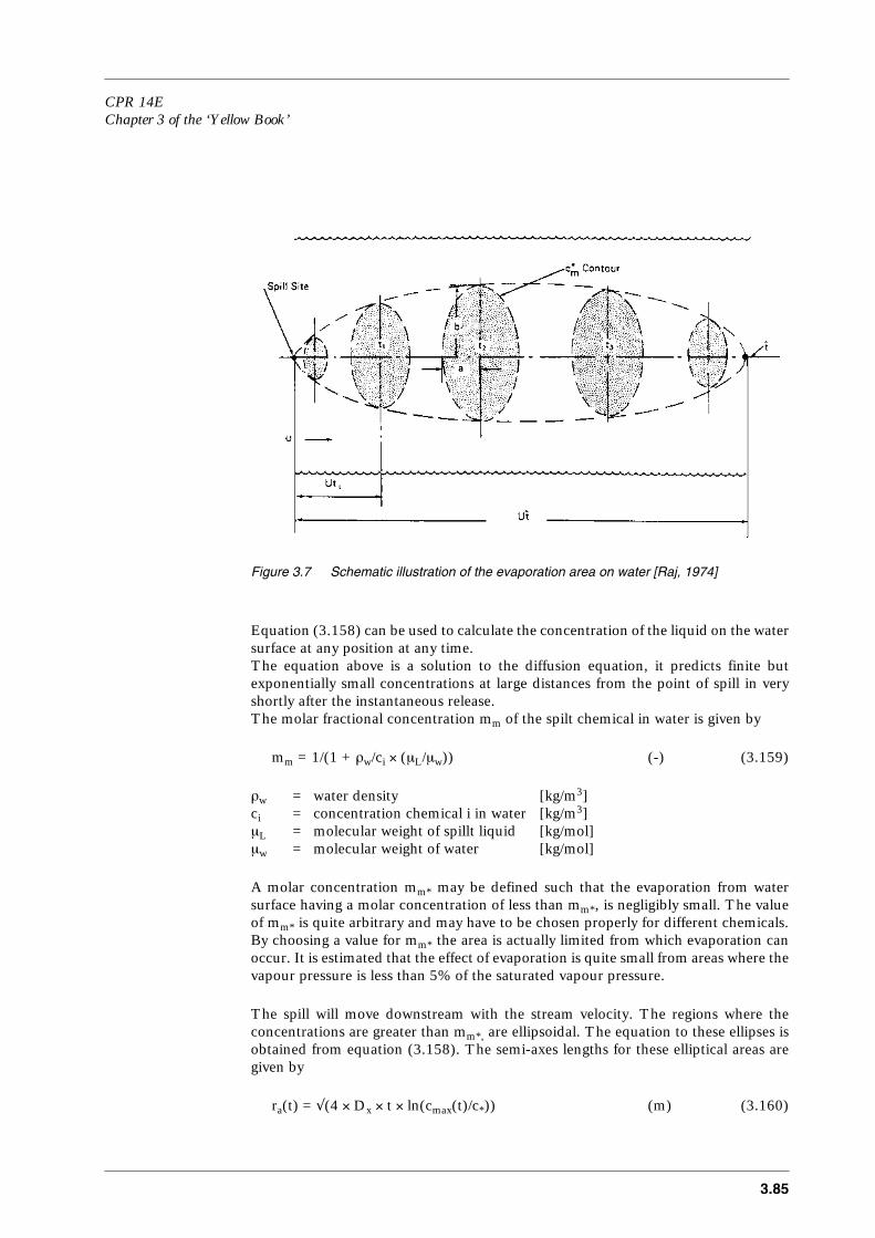
CPR 14EChapter 3 of the ‘Yellow Book’
3.85
Figure 3.7 Schematic illustration of the evaporation area on water [Raj, 1974]
Equation (3.158) can be used to calculate the concentration of the liquid on the watersurface at any position at any time. The equation above is a solution to the diffusion equation, it predicts finite butexponentially small concentrations at large distances from the point of spill in veryshortly after the instantaneous release. The molar fractional concentration mm of the spilt chemical in water is given by
mm = 1/(1 + ρw/ci × (µL/µw)) (-) (3.159)
ρw = water density [kg/m3]ci = concentration chemical i in water [kg/m3]µL = molecular weight of spillt liquid [kg/mol]µw = molecular weight of water [kg/mol]
A molar concentration mm* may be defined such that the evaporation from watersurface having a molar concentration of less than mm*, is negligibly small. The valueof mm* is quite arbitrary and may have to be chosen properly for different chemicals.By choosing a value for mm* the area is actually limited from which evaporation canoccur. It is estimated that the effect of evaporation is quite small from areas where thevapour pressure is less than 5% of the saturated vapour pressure.
The spill will move downstream with the stream velocity. The regions where theconcentrations are greater than mm*, are ellipsoidal. The equation to these ellipses isobtained from equation (3.158). The semi-axes lengths for these elliptical areas aregiven by
ra(t) = √(4 × Dx × t × ln(cmax(t)/c*)) (m) (3.160)
3.86
rb(t) = √(4 × Dy × t × ln(cmax(t)/c*)) (m) (3.161)
where c* is the limiting concentration in units of mass/volume, which is a more or lessarbitrarily value that may be related to flammability limits or toxicity limits.
At the centre of the elliptical area the concentration is a maximum and is given by
If now tc < lim is set equal to the time beyond which the concentration in water of theliquid spilt is below mm* everywhere in the water, then the so-called characteristictime can be calculated by
tc<lim = 1/(4 × π) × (2 × QL/(c* × √(Dx × Dy × Dz)))2/3 (s) (3.163)
The rate of evaporation per unit area q"v may be expressed by
q"v = km,P × Pv,i (3.164)
wherekm,p = mass transfer coefficient related to partial pressure [s/m]
note that
q"v = km × ci (kg/(m2⋅s))
wherekm = mass transfer coefficient related to concentration [m/s]
Applying ideal gas law, it can easily be derived that
km,P = km × µi/(R × T) (s/m) (3.165)
It is assumed that the vapour pressure of the solved chemical follows Raoult’s law bywhich the (partial) vapour concentration is proportional with the molar fraction of thediluted chemical in the water
Pi = mm × Pv˚(T) (N/m2) (3.166)
where Pi is the partial pressure of the vapour of the liquid spillt at the water surface,and Pv˚(T) is the saturated vapour pressure at temperature T.Raoult’s law is quite close to the actual relationship for most chemicals.
So, that
q"v = km,P × mm × Pv˚(T) (kg/(m2⋅s)) (3.167)
ci max, t( )2 QL×
4 π t××( )3/2 Dx Dy Dz××( )×--------------------------------------------------------------------------= (3.162)(kg/m3)

CPR 14EChapter 3 of the ‘Yellow Book’
3.87
The mass transfer coefficient for surface evaporation is estimated from forcedconvection boundary layer theory. The heat mass transfer analogy yields the followingequations for flow over a flat plate
km × L/Da = 1.328 × Sc1/3 × Re1/2 for laminar flow (Re < 5 × 10⁵) (3.168a)
km × L/Da = 0.037 × Sc1/3 × Re0.8 for turbulent flow (Re > 5 × 10⁵) (3.168b)
with
Re = ρa × uw,10 × L/ηa (-) (3.168c)
Sc = υV/Dv (-) (3.25)
≈ 0.8
whereci = atmospheric vapour concentration just [kg/m3] at the evaporating pool surfaceDa = diffusion coefficient chemical in air [m2/s]km = mass transfer coefficient related to concentration [m/s]L = characteristic length of the spill [m]Re = Reynold number [-]Sc = Schmidt number [-]υV = kinematic vapour viscosity [m2/s]
The characteristic length used here is the length of spill which is defined by
L = Vi1/3 (m) (3.169)
where Vi is the initial spill volume. It is assumed that the mass transfer will not changein spite of the fact that the pool is expanding.
Integrating equation (3.167) over the vaporisation area (3.160/161) results in anexpression for the total evaporation rate at any instant
The integral should be taken over the elliptical area on whose boundary theconcentration is mm*. It can be shown that
with
mm,mean = (mm,max - mm)/ln(mm,max/mm*) (-) (3.172)
qv km ,P Pv0 mm dA×
0
A
∫××= (3.170)(kg/s)
mm dA×
0
A
∫ π ra rb mmmean×××= (3.171)(m2)
3.88
Note that ra and rb, representing the dimensions of the ellipsoidal evaporation area onthe water surface, are given by equations (3.160/161).
Combining equations (3.170) and (3.171) yields
qv = π × km,P × Pv˚ × ra × rb × mm,mean (kg/s) (3.173)
Defining the following characteristic values
qch = 4 × π × tc<lim × √(Dx × Dy) × km,P × Pv˚(T) (kg/s) (3.174)
Qch = qch × tc<lim (kg) (3.175)
τ = t/tc<lim (-) (3.176)
QR = Qv/Qch (-) (3.177)
Qv = mass of vapour evolved [kg]Qch = characteristic vapour mass [kg]QR = dimensionless mass of evolved vapour [-]
and noting that
qR = qv/qch (-) (3.178)
qR = dimensionless evaporation rate [-]qch = characteristic evaporation rate [kg/s]qv = liquid evaporation rate [kg/s]
Using equations (3.173), (3.160/161), and (3.163), results in
qR(τ) = -3/2 × τ × ln(τ) × mm,mean(τ) (-) (3.179)
The total mass of vapour Qv evolved up to time tc<lim is given by
Qv = QR × Qch (kg) (3.180)
with
QR = qR × dτ = -3/2 × τ × ln(τ) × mm.mean(τ) × dτ (3.181)
The evaluation of the integral in equation (3.181) has to be done numerically becauseof the complicated nature of the integral. However, certain observations can be madefrom the equation.
It is evident that mm,mean ≥ mm*, so that replacing the value of mm,mean by mm* resultsin a minimum value for m
QR,min = 3/8 × mm* (-) (3.182)
0
1
∫0
1
∫
CPR 14EChapter 3 of the ‘Yellow Book’
3.89
Similarly, by replacing mm,mean by mm,max corresponding to the maximum molarconcentration, the maximum value for QR can be shown to be
QR,max = -3/2 × τ × ln(τ)/1 + ρw × µL × τ3/2/(c* × µw) × dτ (-) (3.183)
If mm,mean is replaced by 1, which would be the absolute maximum value forconcentration, then the maximum evaporation m would be equal to 3/8. Then themaximum possible evaporation is set by
Qv = 3/8 × Qch (kg) (3.184)
The maximum distance where vapour may evolve from the water surface having aconcentration larger than the limiting concentration mm*, is given by
xc<lim = u × tc<lim (m) (3.185)
3.5.6.3 Remarks
The model given is based on mixing and dilution in water of a spillt liquidand a relatively small amount of evaporation caused by the difference of vapourconcentration at the water surface and the atmosphere. It has been assumed that allof the liquid would go into solution. This assumption is valid because it appears thatthe total vapour generated is a small fraction of the mass spillt. This is because even though the evaporation is high, in case of a high partial vapourpressure of the spillt chemical, the duration for which vaporisation can occur isprimarily determined by the rapidity of mixing of the liquid in water. The moreturbulent a stream is, the better the mixing, and the quicker the time in which theconcentration everywhere in the water is less than the critical. In reality the release of chemical takes place in a finite period. Since even in the caseof an instantaneous spill, the mass of vapour evolved appears a small fraction of themass spillt, the predictions can be regarded safely as the worst case for long durationspills. It should be kept in mind that any vaporisation of the spillt liquid during therelease process before water contact, has not been taken into account.
3.5.6.4 Releases of ammonia
Ammonia is an industrial commodity soluble in water, but the release ofammonia onto water can not be expected to solve in the water to the full amount ofthe release.Ammonia spillt onto water will solve or react to ammonium hydroxide (matter ofdefinition) generating a relatively large amount of heat, by the reaction
+ H2O(l) = (NH4+)aq + (OH-)aq
According to Raj and Reid, for an instantaneous ammonia release, about 30% of thespill will evolve from the water surface immediately due to vigorous boiling caused bythe reaction heat or mixing heat generated [Melhelm, 1993].
0
1
∫
NH3 l( )
3.90
However, this was based on small-scale experiments. But according to Raj in hischapter ‘Volatile liquids’ in the Hazardous Material Spills Handbook, part 4‘Ammonia’, in larger spills approximately 50 percent of the spillt liquid vaporised.
This indicates the effects of the dynamics of a spill on vaporisation.So, it is advisable to assume that on average about 40% of a spill will evaporateimmediately. This fraction has been used in other studies that are not publiclyavailable.The remaining 60% of the spill will solve into the water, and will evaporate gradually,and model HACS-R may be applied for this part of the ammonia spill. Note that theammonium hydroxide solution will be warm, and will disperse in the water as a stablystratified fluid. This effect has not been taken into account in the model. Perhapsneedless to say, that for short duration releases the flashing of the cryogen ammoniafrom the water surface has to be taken into account.
Proper estimation of vapour pressures of the components in the solution is critical,since this property has a large and direct effect on the evaporation rate. In multi-component spills the partial vapour pressure depends on the composition of themixture.For multi-component liquid pools the evaporation rate will decrease in time also dueto the change in composition, while the most volatile components will evaporate first.So, the vapour pressure is dependent on the composition.For an ammonia-water mixture the following correlations have been derived[Mikesell, 1993]:
ln(Pv,NH3/101325.) = 17.17 - 4294/T + 0.1370 × mw,NH3 - 0.00347 × mw,NH32
+ 23.01 × mw,NH3 /T (-) (3.186a)
ln(Pv,H2O/101325.) = 18.37 - 4552/T + 0.1477 × mw,NH3 - 0.00081 × ww,NH32
- 43.53 × mw,NH3 /T (-) (3.186b)
mw,NH3 = mass fraction solved ammonia in water [kg/kg]T = absolute temperature ammonia-water mixture [K]Pv,NH3 = partial vapour pressure ammonia [N/m2]Pv,H2O = partial vapour pressure water [N/m2]
Note1 atm = 101325 N/m2.

CPR 14EChapter 3 of the ‘Yellow Book’
3.91
3.6 Application of the selected models: calculation examples
3.6.1 Introduction to section 3.6
Some models presented in subsection 3.5, HACS-R and especially GASP,are rather complex models. It is practically not possible to perform the calculationsby hand or step by step.
Section 3.6 provides examples using the models and methods described in section3.5. Subsection 3.6.2 provides example calculations with the GASP model for thespreading of liquids on solid subsoil and water, presented in 3.5.2.Subsection 3.6.3 provides example calculations with the HACS-R model for spills ofvolatile liquids that solve in water, as presented in 3.5.6.Subsection 3.6.4 provides example calculations for various supplementary models ashas been addressed in section 3.5.
3.6.2 Calculation example GASP
Introduction
GASP models an instantaneous spill of liquid chlorine released from a tank railwaywagon onto land. The pool spread is unrestricted.The initial, cylindrical, pool of chlorine has a radius of 9.16 m (area 263.597 m2) andvolume 65.95 m3 (implying a depth of 0.250192 m). The rate at which the pool willevaporate is calculated by GASP from knowledge of the ground properties and theatmospheric conditions. The release temperature (239.12 K) is also important. Heatis being transfered from the ground (conductivity 2.5 W/(m⋅K), diffusivity 11 m2/s)into the pool. Perfect thermal contact is assumed.The atmospheric temperature is 15 ˚C and the windspeed is 1.5 m/s.The net solar radiation can be estimated by equations (4.36) and (4.37) presented inchapter 4 ‘Vapour cloud dispersion’.However, for the sake of simplicity a value of 100 kW/m2 has been chosen.
Initial pool conditions
Initial volume of pool V = 65.95 m3
Initial radius of pool r = 9.160 mInitial depth of pool h = 0.2502 mInitial front velocity u = 0.0000 m/sInitial temperature T0 = 238.1 K
Atmospheric conditions
Wind speed at 10 metres ua,10 = 1.500 m/sAmbient temperature Ta = 288.2 KAtmospheric friction velocity u* = 8.6859E-02 m/sRoughness length z0,a = 1.0000E-02 mThe pool has roughness length z0,p = 2.3000E-04 m
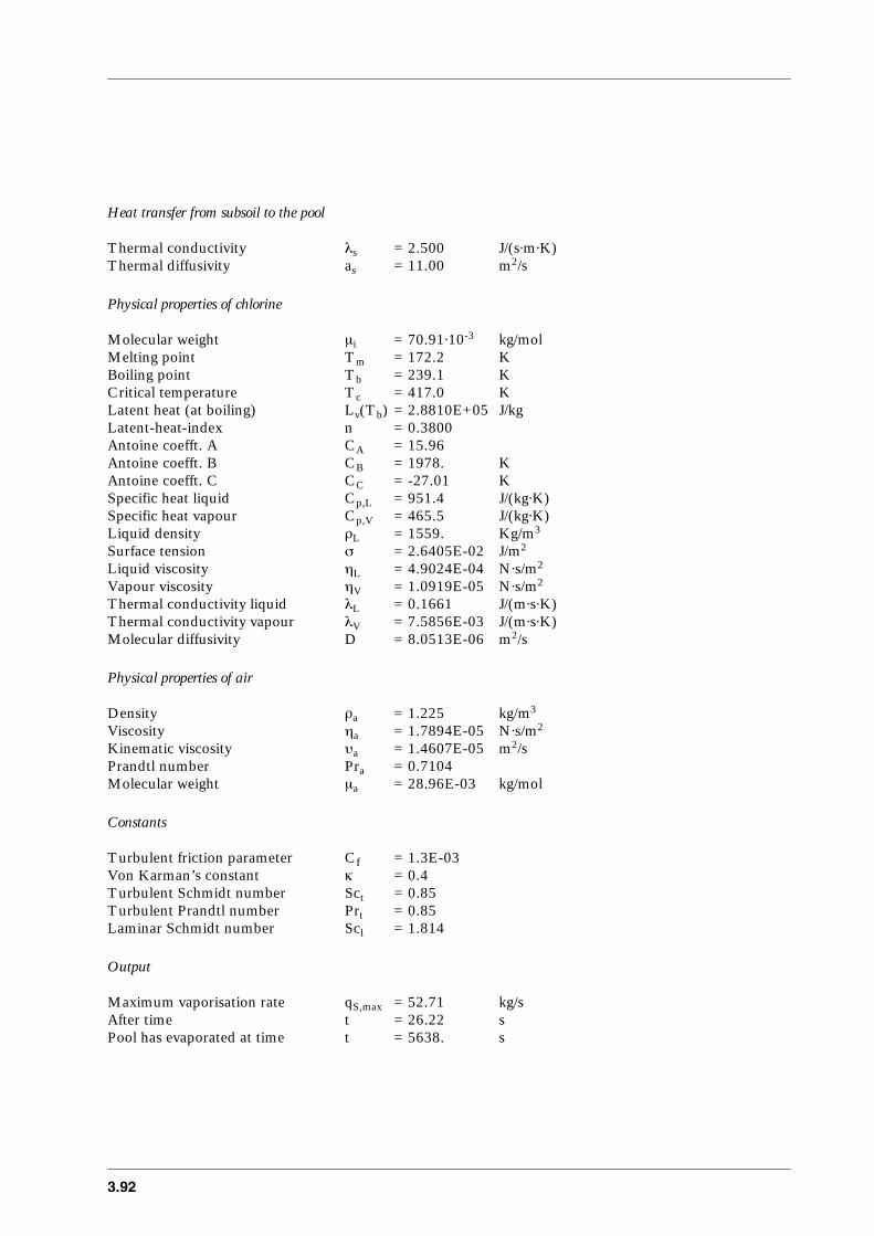
3.92
Heat transfer from subsoil to the pool
Thermal conductivity λs = 2.500 J/(s⋅m⋅K)Thermal diffusivity as = 11.00 m2/s
Physical properties of chlorine
Molecular weight µi = 70.91⋅10-3 kg/molMelting point Tm = 172.2 KBoiling point Tb = 239.1 KCritical temperature Tc = 417.0 KLatent heat (at boiling) Lv(Tb) = 2.8810E+05 J/kgLatent-heat-index n = 0.3800Antoine coefft. A CA = 15.96Antoine coefft. B CB = 1978. KAntoine coefft. C CC = -27.01 KSpecific heat liquid Cp,L = 951.4 J/(kg⋅K)Specific heat vapour Cp,V = 465.5 J/(kg⋅K)Liquid density ρL = 1559. Kg/m3
Surface tension σ = 2.6405E-02 J/m2
Liquid viscosity ηL = 4.9024E-04 N⋅s/m2
Vapour viscosity ηV = 1.0919E-05 N⋅s/m2
Thermal conductivity liquid λL = 0.1661 J/(m⋅s⋅K)Thermal conductivity vapour λV = 7.5856E-03 J/(m⋅s⋅K)Molecular diffusivity D = 8.0513E-06 m2/s
Physical properties of air
Density ρa = 1.225 kg/m3
Viscosity ηa = 1.7894E-05 N⋅s/m2
Kinematic viscosity υa = 1.4607E-05 m2/sPrandtl number Pra = 0.7104Molecular weight µa = 28.96E-03 kg/mol
Constants
Turbulent friction parameter Cf = 1.3E-03Von Karman’s constant κ = 0.4Turbulent Schmidt number Sct = 0.85Turbulent Prandtl number Prt = 0.85Laminar Schmidt number Scl = 1.814
Output
Maximum vaporisation rate qS,max = 52.71 kg/sAfter time t = 26.22 sPool has evaporated at time t = 5638. s

CPR 14EChapter 3 of the ‘Yellow Book’
3.93
t(s)
r(m)
Qv(kg)
h(m)
Vd(m3)
0.0000 9.160 0.0000 0.2502 65.952.8482E-07 9.160 1.9688E-06 0.2502 65.955.6965E-07 9.160 3.9377E-06 0.2502 65.958.5447E-07 9.160 5.9065E-06 0.2502 65.953.5060E-06 9.160 2.4235E-05 0.2502 65.956.1575E-06 9.160 4.2563E-05 0.2502 65.958.8090E-06 9.160 6.0891E-05 0.2502 65.952.4248E-05 9.160 1.6761E-04 0.2502 65.953.9687E-05 9.160 2.7433E-04 0.2502 65.955.5125E-05 9.160 3.8105E-04 0.2502 65.951.1684E-04 9.160 8.0767E-04 0.2502 65.951.7856E-04 9.160 1.2343E-03 0.2502 65.952.4028E-04 9.160 1.6609E-03 0.2502 65.954.2861E-04 9.160 2.9627E-03 0.2502 65.956.1694E-04 9.160 4.2645E-03 0.2502 65.958.0527E-04 9.160 5.5664E-03 0.2502 65.951.2764E-03 9.160 8.8229E-03 0.2502 65.951.7475E-03 9.160 1.2079E-02 0.2502 65.952.2186E-03 9.160 1.5336E-02 0.2502 65.953.2082E-03 9.160 2.2177E-02 0.2502 65.954.1979E-03 9.160 2.9017E-02 0.2502 65.955.1875E-03 9.160 3.5858E-02 0.2502 65.957.0839E-03 9.160 4.8966E-02 0.2502 65.958.9802E-03 9.160 6.2074E-02 0.2502 65.951.0877E-02 9.160 7.5182E-02 0.2502 65.951.2773E-02 9.160 8.8290E-02 0.2502 65.951.7217E-02 9.160 0.1190 0.2502 65.952.1662E-02 9.160 0.1497 0.2502 65.952.6106E-02 9.160 0.1804 0.2502 65.953.0551E-02 9.161 0.2112 0.2502 65.953.9682E-02 9.161 0.2743 0.2501 65.954.8813E-02 9.161 0.3374 0.2501 65.955.7944E-02 9.162 0.4005 0.2501 65.956.7076E-02 9.162 0.4636 0.2501 65.958.2946E-02 9.164 0.5734 0.2500 65.959.8816E-02 9.165 0.6831 0.2499 65.950.1147 9.167 0.7929 0.2498 65.950.1306 9.169 0.9027 0.2497 65.950.1594 9.174 1.102 0.2494 65.950.1882 9.179 1.302 0.2492 65.950.2170 9.185 1.502 0.2488 65.950.2458 9.192 1.702 0.2484 65.950.2746 9.200 1.902 0.2480 65.950.3227 9.216 2.237 0.2472 65.95
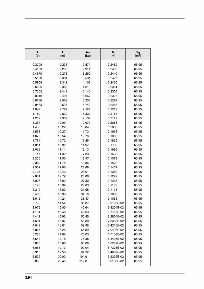
3.94
0.3708 9.233 2.574 0.2462 65.950.4189 9.253 2.911 0.2452 65.950.4670 9.276 3.250 0.2440 65.950.5150 9.301 3.591 0.2427 65.950.5868 9.342 4.103 0.2405 65.950.6585 9.389 4.619 0.2381 65.950.7302 9.441 5.140 0.2355 65.950.8019 9.497 5.667 0.2327 65.950.8736 9.559 6.200 0.2297 65.950.9453 9.625 6.740 0.2266 65.951.047 9.727 7.522 0.2218 65.951.150 9.839 8.322 0.2168 65.951.252 9.959 9.139 0.2117 65.951.354 10.09 9.977 0.2063 65.951.456 10.22 10.84 0.2008 65.951.558 10.37 11.72 0.1953 65.951.676 10.54 12.76 0.1889 65.951.794 10.72 13.85 0.1825 65.951.911 10.92 14.97 0.1762 65.952.029 11.11 16.13 0.1699 65.952.147 11.32 17.33 0.1638 65.952.265 11.53 18.57 0.1578 65.952.382 11.75 19.86 0.1520 65.952.559 12.08 21.88 0.1437 65.952.735 12.43 24.01 0.1359 65.952.881 12.72 25.86 0.1297 65.953.027 13.02 27.80 0.1238 65.953.173 13.32 29.83 0.1183 65.953.319 13.62 31.95 0.1131 65.953.465 13.93 34.16 0.1082 65.953.612 14.24 36.47 0.1035 65.953.758 14.54 38.87 9.9198E-02 65.953.976 15.00 42.64 9.3204E-02 65.954.194 15.46 46.63 8.7755E-02 65.954.412 15.92 50.85 8.2804E-02 65.954.631 16.37 55.30 7.8305E-02 65.954.849 16.81 59.98 7.4216E-02 65.955.067 17.25 64.89 7.0496E-02 65.955.285 17.68 70.03 6.7108E-02 65.955.543 18.18 76.38 6.3495E-02 65.955.800 18.66 83.06 6.0249E-02 65.956.058 19.13 90.04 5.7326E-02 65.956.315 19.58 97.32 5.4689E-02 65.956.572 20.02 104.9 5.2302E-02 65.956.830 20.45 112.8 5.0138E-02 65.95
t(s)
r(m)
Qv(kg)
h(m)
Vd(m3)
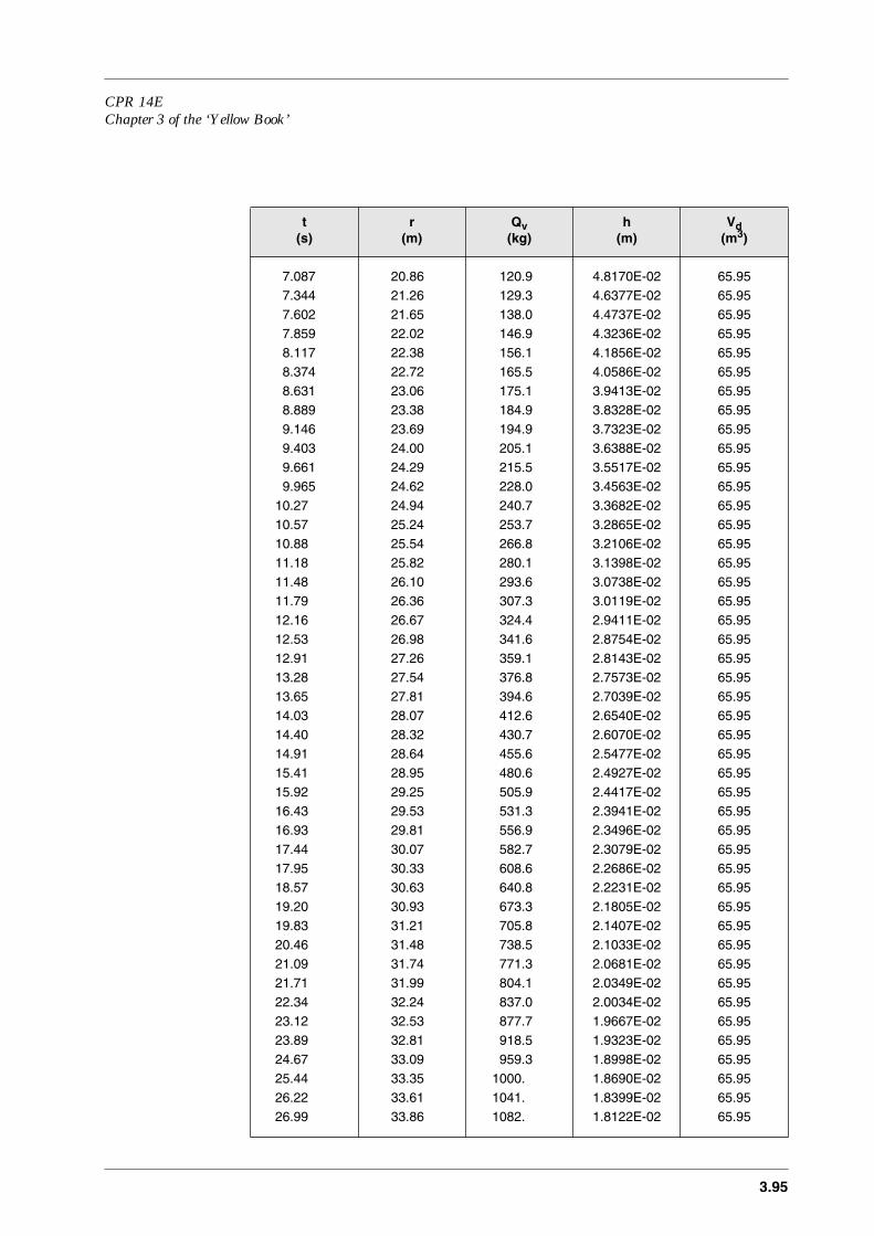
CPR 14EChapter 3 of the ‘Yellow Book’
3.95
7.087 20.86 120.9 4.8170E-02 65.957.344 21.26 129.3 4.6377E-02 65.957.602 21.65 138.0 4.4737E-02 65.957.859 22.02 146.9 4.3236E-02 65.958.117 22.38 156.1 4.1856E-02 65.958.374 22.72 165.5 4.0586E-02 65.958.631 23.06 175.1 3.9413E-02 65.958.889 23.38 184.9 3.8328E-02 65.959.146 23.69 194.9 3.7323E-02 65.959.403 24.00 205.1 3.6388E-02 65.959.661 24.29 215.5 3.5517E-02 65.959.965 24.62 228.0 3.4563E-02 65.95
10.27 24.94 240.7 3.3682E-02 65.9510.57 25.24 253.7 3.2865E-02 65.9510.88 25.54 266.8 3.2106E-02 65.9511.18 25.82 280.1 3.1398E-02 65.9511.48 26.10 293.6 3.0738E-02 65.9511.79 26.36 307.3 3.0119E-02 65.9512.16 26.67 324.4 2.9411E-02 65.9512.53 26.98 341.6 2.8754E-02 65.9512.91 27.26 359.1 2.8143E-02 65.9513.28 27.54 376.8 2.7573E-02 65.9513.65 27.81 394.6 2.7039E-02 65.9514.03 28.07 412.6 2.6540E-02 65.9514.40 28.32 430.7 2.6070E-02 65.9514.91 28.64 455.6 2.5477E-02 65.9515.41 28.95 480.6 2.4927E-02 65.9515.92 29.25 505.9 2.4417E-02 65.9516.43 29.53 531.3 2.3941E-02 65.9516.93 29.81 556.9 2.3496E-02 65.9517.44 30.07 582.7 2.3079E-02 65.9517.95 30.33 608.6 2.2686E-02 65.9518.57 30.63 640.8 2.2231E-02 65.9519.20 30.93 673.3 2.1805E-02 65.9519.83 31.21 705.8 2.1407E-02 65.9520.46 31.48 738.5 2.1033E-02 65.9521.09 31.74 771.3 2.0681E-02 65.9521.71 31.99 804.1 2.0349E-02 65.9522.34 32.24 837.0 2.0034E-02 65.9523.12 32.53 877.7 1.9667E-02 65.9523.89 32.81 918.5 1.9323E-02 65.9524.67 33.09 959.3 1.8998E-02 65.9525.44 33.35 1000. 1.8690E-02 65.9526.22 33.61 1041. 1.8399E-02 65.9526.99 33.86 1082. 1.8122E-02 65.95
t(s)
r(m)
Qv(kg)
h(m)
Vd(m3)

3.96
27.77 34.10 1123. 1.7858E-02 65.9528.73 34.39 1174. 1.7546E-02 65.9529.70 34.68 1224. 1.7251E-02 65.9530.66 34.95 1275. 1.6972E-02 65.9531.63 35.22 1326. 1.6706E-02 65.9532.59 35.48 1376. 1.6453E-02 65.9533.56 35.73 1427. 1.6211E-02 65.9534.53 35.98 1477. 1.5980E-02 65.9535.68 36.27 1537. 1.5716E-02 65.9536.84 36.56 1598. 1.5465E-02 65.9538.00 36.83 1657. 1.5225E-02 65.9539.16 37.10 1717. 1.4997E-02 65.9540.32 37.36 1777. 1.4778E-02 65.9541.48 37.62 1836. 1.4568E-02 65.9542.63 37.87 1895. 1.4367E-02 65.9544.24 38.21 1977. 1.4101E-02 65.9545.84 38.54 2058. 1.3849E-02 65.9547.45 38.86 2138. 1.3610E-02 65.9549.05 39.18 2219. 1.3382E-02 65.9550.66 39.48 2299. 1.3164E-02 65.9552.26 39.78 2378. 1.2956E-02 65.9553.86 40.08 2457. 1.2758E-02 65.9555.94 40.45 2558. 1.2513E-02 65.9558.01 40.81 2659. 1.2281E-02 65.9560.08 41.16 2759. 1.2061E-02 65.9562.15 41.50 2858. 1.1851E-02 65.9564.23 41.83 2956. 1.1651E-02 65.9566.30 42.16 3054. 1.1461E-02 65.9568.37 42.48 3151. 1.1278E-02 65.9571.12 42.89 3278. 1.1048E-02 65.9573.87 43.29 3405. 1.0830E-02 65.9576.61 43.68 3530. 1.0624E-02 65.9579.36 44.06 3653. 1.0428E-02 65.9582.11 44.44 3776. 1.0241E-02 65.9584.86 44.80 3897. 1.0064E-02 65.9587.60 45.15 4017. 9.8940E-03 65.9591.17 45.60 4171. 9.6850E-03 65.9594.73 46.04 4324. 9.4875E-03 65.9598.29 46.46 4474. 9.3004E-03 65.95
101.9 46.88 4622. 9.1228E-03 65.95105.4 47.28 4769. 8.9541E-03 65.95109.0 47.68 4914. 8.7934E-03 65.95112.6 48.06 5057. 8.6402E-03 65.95117.2 48.55 5241. 8.4506E-03 65.95121.9 49.03 5423. 8.2715E-03 65.95
t(s)
r(m)
Qv(kg)
h(m)
Vd(m3)
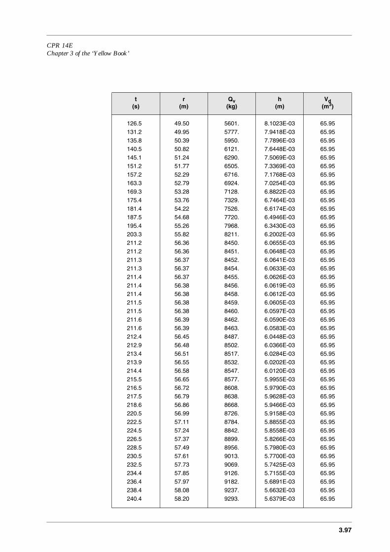
CPR 14EChapter 3 of the ‘Yellow Book’
3.97
126.5 49.50 5601. 8.1023E-03 65.95131.2 49.95 5777. 7.9418E-03 65.95135.8 50.39 5950. 7.7896E-03 65.95140.5 50.82 6121. 7.6448E-03 65.95145.1 51.24 6290. 7.5069E-03 65.95151.2 51.77 6505. 7.3369E-03 65.95157.2 52.29 6716. 7.1768E-03 65.95163.3 52.79 6924. 7.0254E-03 65.95169.3 53.28 7128. 6.8822E-03 65.95175.4 53.76 7329. 6.7464E-03 65.95181.4 54.22 7526. 6.6174E-03 65.95187.5 54.68 7720. 6.4946E-03 65.95195.4 55.26 7968. 6.3430E-03 65.95203.3 55.82 8211. 6.2002E-03 65.95211.2 56.36 8450. 6.0655E-03 65.95211.2 56.36 8451. 6.0648E-03 65.95211.3 56.37 8452. 6.0641E-03 65.95211.3 56.37 8454. 6.0633E-03 65.95211.4 56.37 8455. 6.0626E-03 65.95211.4 56.38 8456. 6.0619E-03 65.95211.4 56.38 8458. 6.0612E-03 65.95211.5 56.38 8459. 6.0605E-03 65.95211.5 56.38 8460. 6.0597E-03 65.95211.6 56.39 8462. 6.0590E-03 65.95211.6 56.39 8463. 6.0583E-03 65.95212.4 56.45 8487. 6.0448E-03 65.95212.9 56.48 8502. 6.0366E-03 65.95213.4 56.51 8517. 6.0284E-03 65.95213.9 56.55 8532. 6.0202E-03 65.95214.4 56.58 8547. 6.0120E-03 65.95215.5 56.65 8577. 5.9955E-03 65.95216.5 56.72 8608. 5.9790E-03 65.95217.5 56.79 8638. 5.9628E-03 65.95218.6 56.86 8668. 5.9466E-03 65.95220.5 56.99 8726. 5.9158E-03 65.95222.5 57.11 8784. 5.8855E-03 65.95224.5 57.24 8842. 5.8558E-03 65.95226.5 57.37 8899. 5.8266E-03 65.95228.5 57.49 8956. 5.7980E-03 65.95230.5 57.61 9013. 5.7700E-03 65.95232.5 57.73 9069. 5.7425E-03 65.95234.4 57.85 9126. 5.7155E-03 65.95236.4 57.97 9182. 5.6891E-03 65.95238.4 58.08 9237. 5.6632E-03 65.95240.4 58.20 9293. 5.6379E-03 65.95
t(s)
r(m)
Qv(kg)
h(m)
Vd(m3)

3.98
242.4 58.31 9348. 5.6130E-03 65.95244.4 58.42 9403. 5.5887E-03 65.95246.4 58.53 9458. 5.5648E-03 65.95248.3 58.63 9512. 5.5415E-03 65.95251.7 58.81 9604. 5.5028E-03 65.95255.1 58.98 9695. 5.4654E-03 65.95258.5 59.15 9785. 5.4292E-03 65.95261.8 59.31 9875. 5.3941E-03 65.95265.2 59.47 9963. 5.3601E-03 65.95268.6 59.63 1.0052E+04 5.3272E-03 65.95274.0 59.87 1.0191E+04 5.2764E-03 65.95279.4 60.10 1.0329E+04 5.2279E-03 65.95284.8 60.33 1.0465E+04 5.1815E-03 65.95290.2 60.54 1.0600E+04 5.1371E-03 65.95295.6 60.75 1.0732E+04 5.0943E-03 65.95300.9 60.95 1.0864E+04 5.0533E-03 65.95308.7 61.23 1.1050E+04 4.9969E-03 65.95316.4 61.50 1.1233E+04 4.9434E-03 65.95324.2 61.76 1.1413E+04 4.8924E-03 65.95331.9 62.01 1.1590E+04 4.8438E-03 65.95339.7 62.25 1.1764E+04 4.7973E-03 65.95347.4 62.48 1.1936E+04 4.7528E-03 65.95356.6 62.75 1.2137E+04 4.7023E-03 65.95365.8 63.00 1.2334E+04 4.6542E-03 65.95374.9 63.25 1.2528E+04 4.6082E-03 65.95384.1 63.49 1.2720E+04 4.5642E-03 65.95393.3 63.72 1.2908E+04 4.5219E-03 65.95402.5 63.94 1.3094E+04 4.4813E-03 65.95411.6 64.15 1.3277E+04 4.4422E-03 65.95426.4 64.49 1.3568E+04 4.3822E-03 65.95441.2 64.80 1.3852E+04 4.3255E-03 65.95455.9 65.11 1.4132E+04 4.2718E-03 65.95470.7 65.40 1.4406E+04 4.2208E-03 65.95485.5 65.68 1.4677E+04 4.1722E-03 65.95500.2 65.95 1.4943E+04 4.1258E-03 65.95515.0 66.20 1.5205E+04 4.0814E-03 65.95532.7 66.50 1.5515E+04 4.0306E-03 65.95550.5 66.79 1.5821E+04 3.9822E-03 65.95568.2 67.06 1.6123E+04 3.9361E-03 65.95585.9 67.32 1.6421E+04 3.8919E-03 65.95603.6 67.58 1.6715E+04 3.8496E-03 65.95621.4 67.82 1.7007E+04 3.8089E-03 65.95639.1 68.06 1.7296E+04 3.7698E-03 65.95653.6 68.25 1.7531E+04 3.7388E-03 65.95668.2 68.43 1.7765E+04 3.7086E-03 65.95
t(s)
r(m)
Qv(kg)
h(m)
Vd(m3)
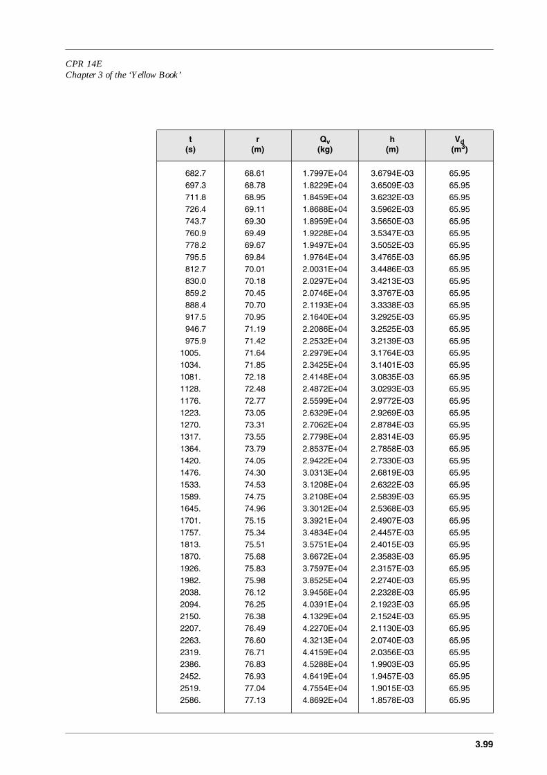
CPR 14EChapter 3 of the ‘Yellow Book’
3.99
682.7 68.61 1.7997E+04 3.6794E-03 65.95697.3 68.78 1.8229E+04 3.6509E-03 65.95711.8 68.95 1.8459E+04 3.6232E-03 65.95726.4 69.11 1.8688E+04 3.5962E-03 65.95743.7 69.30 1.8959E+04 3.5650E-03 65.95760.9 69.49 1.9228E+04 3.5347E-03 65.95778.2 69.67 1.9497E+04 3.5052E-03 65.95795.5 69.84 1.9764E+04 3.4765E-03 65.95812.7 70.01 2.0031E+04 3.4486E-03 65.95830.0 70.18 2.0297E+04 3.4213E-03 65.95859.2 70.45 2.0746E+04 3.3767E-03 65.95888.4 70.70 2.1193E+04 3.3338E-03 65.95917.5 70.95 2.1640E+04 3.2925E-03 65.95946.7 71.19 2.2086E+04 3.2525E-03 65.95975.9 71.42 2.2532E+04 3.2139E-03 65.95
1005. 71.64 2.2979E+04 3.1764E-03 65.951034. 71.85 2.3425E+04 3.1401E-03 65.951081. 72.18 2.4148E+04 3.0835E-03 65.951128. 72.48 2.4872E+04 3.0293E-03 65.951176. 72.77 2.5599E+04 2.9772E-03 65.951223. 73.05 2.6329E+04 2.9269E-03 65.951270. 73.31 2.7062E+04 2.8784E-03 65.951317. 73.55 2.7798E+04 2.8314E-03 65.951364. 73.79 2.8537E+04 2.7858E-03 65.951420. 74.05 2.9422E+04 2.7330E-03 65.951476. 74.30 3.0313E+04 2.6819E-03 65.951533. 74.53 3.1208E+04 2.6322E-03 65.951589. 74.75 3.2108E+04 2.5839E-03 65.951645. 74.96 3.3012E+04 2.5368E-03 65.951701. 75.15 3.3921E+04 2.4907E-03 65.951757. 75.34 3.4834E+04 2.4457E-03 65.951813. 75.51 3.5751E+04 2.4015E-03 65.951870. 75.68 3.6672E+04 2.3583E-03 65.951926. 75.83 3.7597E+04 2.3157E-03 65.951982. 75.98 3.8525E+04 2.2740E-03 65.952038. 76.12 3.9456E+04 2.2328E-03 65.952094. 76.25 4.0391E+04 2.1923E-03 65.952150. 76.38 4.1329E+04 2.1524E-03 65.952207. 76.49 4.2270E+04 2.1130E-03 65.952263. 76.60 4.3213E+04 2.0740E-03 65.952319. 76.71 4.4159E+04 2.0356E-03 65.952386. 76.83 4.5288E+04 1.9903E-03 65.952452. 76.93 4.6419E+04 1.9457E-03 65.952519. 77.04 4.7554E+04 1.9015E-03 65.952586. 77.13 4.8692E+04 1.8578E-03 65.95
t(s)
r(m)
Qv(kg)
h(m)
Vd(m3)
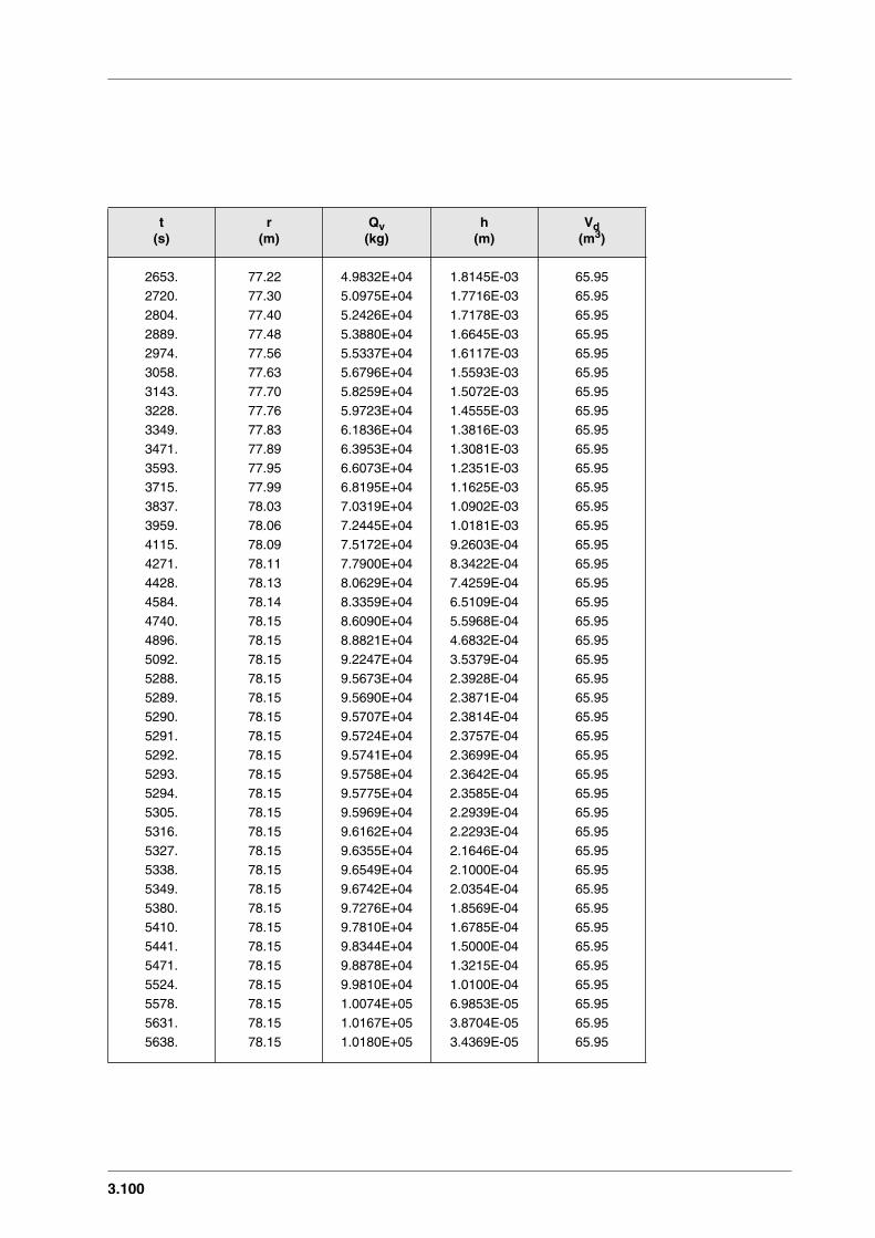
3.100
2653. 77.22 4.9832E+04 1.8145E-03 65.952720. 77.30 5.0975E+04 1.7716E-03 65.952804. 77.40 5.2426E+04 1.7178E-03 65.952889. 77.48 5.3880E+04 1.6645E-03 65.952974. 77.56 5.5337E+04 1.6117E-03 65.953058. 77.63 5.6796E+04 1.5593E-03 65.953143. 77.70 5.8259E+04 1.5072E-03 65.953228. 77.76 5.9723E+04 1.4555E-03 65.953349. 77.83 6.1836E+04 1.3816E-03 65.953471. 77.89 6.3953E+04 1.3081E-03 65.953593. 77.95 6.6073E+04 1.2351E-03 65.953715. 77.99 6.8195E+04 1.1625E-03 65.953837. 78.03 7.0319E+04 1.0902E-03 65.953959. 78.06 7.2445E+04 1.0181E-03 65.954115. 78.09 7.5172E+04 9.2603E-04 65.954271. 78.11 7.7900E+04 8.3422E-04 65.954428. 78.13 8.0629E+04 7.4259E-04 65.954584. 78.14 8.3359E+04 6.5109E-04 65.954740. 78.15 8.6090E+04 5.5968E-04 65.954896. 78.15 8.8821E+04 4.6832E-04 65.955092. 78.15 9.2247E+04 3.5379E-04 65.955288. 78.15 9.5673E+04 2.3928E-04 65.955289. 78.15 9.5690E+04 2.3871E-04 65.955290. 78.15 9.5707E+04 2.3814E-04 65.955291. 78.15 9.5724E+04 2.3757E-04 65.955292. 78.15 9.5741E+04 2.3699E-04 65.955293. 78.15 9.5758E+04 2.3642E-04 65.955294. 78.15 9.5775E+04 2.3585E-04 65.955305. 78.15 9.5969E+04 2.2939E-04 65.955316. 78.15 9.6162E+04 2.2293E-04 65.955327. 78.15 9.6355E+04 2.1646E-04 65.955338. 78.15 9.6549E+04 2.1000E-04 65.955349. 78.15 9.6742E+04 2.0354E-04 65.955380. 78.15 9.7276E+04 1.8569E-04 65.955410. 78.15 9.7810E+04 1.6785E-04 65.955441. 78.15 9.8344E+04 1.5000E-04 65.955471. 78.15 9.8878E+04 1.3215E-04 65.955524. 78.15 9.9810E+04 1.0100E-04 65.955578. 78.15 1.0074E+05 6.9853E-05 65.955631. 78.15 1.0167E+05 3.8704E-05 65.955638. 78.15 1.0180E+05 3.4369E-05 65.95
t(s)
r(m)
Qv(kg)
h(m)
Vd(m3)
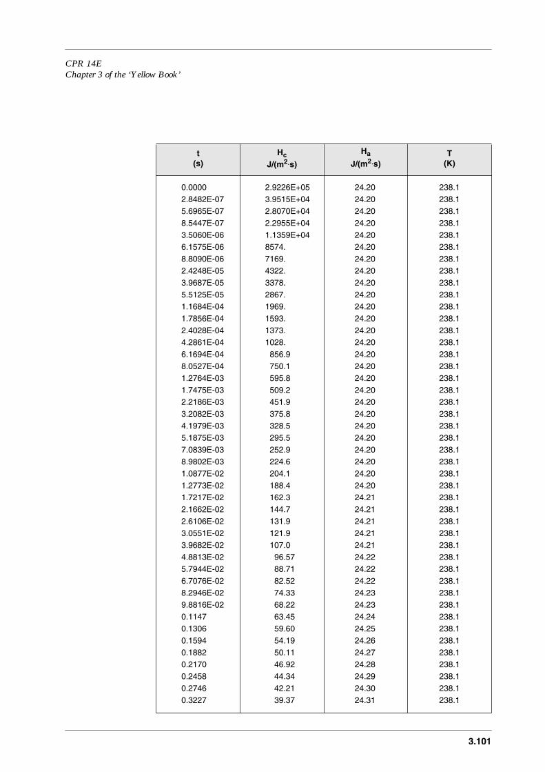
CPR 14EChapter 3 of the ‘Yellow Book’
3.101
t(s)
Hc
J/(m2⋅s)
Ha
J/(m2⋅s)T
(K)
0.0000 2.9226E+05 24.20 238.12.8482E-07 3.9515E+04 24.20 238.15.6965E-07 2.8070E+04 24.20 238.18.5447E-07 2.2955E+04 24.20 238.13.5060E-06 1.1359E+04 24.20 238.16.1575E-06 8574. 24.20 238.18.8090E-06 7169. 24.20 238.12.4248E-05 4322. 24.20 238.13.9687E-05 3378. 24.20 238.15.5125E-05 2867. 24.20 238.11.1684E-04 1969. 24.20 238.11.7856E-04 1593. 24.20 238.12.4028E-04 1373. 24.20 238.14.2861E-04 1028. 24.20 238.16.1694E-04 856.9 24.20 238.18.0527E-04 750.1 24.20 238.11.2764E-03 595.8 24.20 238.11.7475E-03 509.2 24.20 238.12.2186E-03 451.9 24.20 238.13.2082E-03 375.8 24.20 238.14.1979E-03 328.5 24.20 238.15.1875E-03 295.5 24.20 238.17.0839E-03 252.9 24.20 238.18.9802E-03 224.6 24.20 238.11.0877E-02 204.1 24.20 238.11.2773E-02 188.4 24.20 238.11.7217E-02 162.3 24.21 238.12.1662E-02 144.7 24.21 238.12.6106E-02 131.9 24.21 238.13.0551E-02 121.9 24.21 238.13.9682E-02 107.0 24.21 238.14.8813E-02 96.57 24.22 238.15.7944E-02 88.71 24.22 238.16.7076E-02 82.52 24.22 238.18.2946E-02 74.33 24.23 238.19.8816E-02 68.22 24.23 238.10.1147 63.45 24.24 238.10.1306 59.60 24.25 238.10.1594 54.19 24.26 238.10.1882 50.11 24.27 238.1 0.2170 46.92 24.28 238.10.2458 44.34 24.29 238.10.2746 42.21 24.30 238.10.3227 39.37 24.31 238.1

3.102
0.3708 37.17 24.33 238.10.4189 35.41 24.35 238.10.4670 33.98 24.36 238.10.5150 32.79 24.38 238.10.5868 31.37 24.40 238.10.6585 30.25 24.43 238.10.7302 29.35 24.45 238.10.8019 28.61 24.47 238.10.8736 28.01 24.50 238.10.9453 27.51 24.52 238.11.047 26.93 24.56 238.11.150 26.47 24.59 238.11.252 26.09 24.63 238.11.354 25.79 24.66 238.11.456 25.53 24.70 238.11.558 25.32 24.74 238.11.676 25.11 24.78 238.11.794 24.92 24.82 238.11.911 24.76 24.87 238.12.029 24.61 24.92 238.12.147 24.47 24.97 238.12.265 24.33 25.02 238.02.382 24.19 25.07 238.02.559 23.99 25.16 238.02.735 23.78 25.25 238.02.881 23.60 25.33 238.03.027 23.42 25.41 238.03.173 23.22 25.50 238.03.319 23.02 25.59 238.03.465 22.82 25.68 238.03.612 22.61 25.78 238.03.758 22.39 25.89 238.03.976 22.05 26.05 238.04.194 21.71 26.23 238.04.412 21.35 26.41 238.04.631 21.00 26.61 237.94.849 20.64 26.82 237.95.067 20.28 27.04 237.95.285 19.92 27.26 237.95.543 19.50 27.55 237.95.800 19.09 27.84 237.96.058 18.69 28.15 237.86.315 18.29 28.48 237.86.572 17.91 28.81 237.86.830 17.53 29.16 237.8
t(s)
Hc
J/(m2⋅s)
Ha
J/(m2⋅s)T
(K)
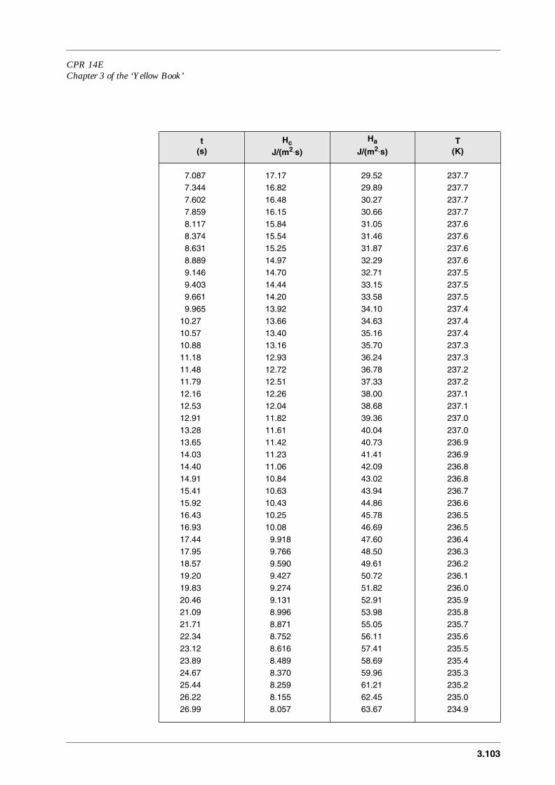
CPR 14EChapter 3 of the ‘Yellow Book’
3.103
7.087 17.17 29.52 237.77.344 16.82 29.89 237.77.602 16.48 30.27 237.77.859 16.15 30.66 237.78.117 15.84 31.05 237.68.374 15.54 31.46 237.68.631 15.25 31.87 237.68.889 14.97 32.29 237.69.146 14.70 32.71 237.59.403 14.44 33.15 237.59.661 14.20 33.58 237.59.965 13.92 34.10 237.4
10.27 13.66 34.63 237.410.57 13.40 35.16 237.410.88 13.16 35.70 237.311.18 12.93 36.24 237.311.48 12.72 36.78 237.211.79 12.51 37.33 237.212.16 12.26 38.00 237.112.53 12.04 38.68 237.112.91 11.82 39.36 237.013.28 11.61 40.04 237.013.65 11.42 40.73 236.914.03 11.23 41.41 236.914.40 11.06 42.09 236.814.91 10.84 43.02 236.815.41 10.63 43.94 236.715.92 10.43 44.86 236.616.43 10.25 45.78 236.516.93 10.08 46.69 236.517.44 9.918 47.60 236.417.95 9.766 48.50 236.318.57 9.590 49.61 236.219.20 9.427 50.72 236.119.83 9.274 51.82 236.020.46 9.131 52.91 235.921.09 8.996 53.98 235.821.71 8.871 55.05 235.722.34 8.752 56.11 235.623.12 8.616 57.41 235.523.89 8.489 58.69 235.424.67 8.370 59.96 235.325.44 8.259 61.21 235.226.22 8.155 62.45 235.026.99 8.057 63.67 234.9
t(s)
Hc
J/(m2⋅s)
Ha
J/(m2⋅s)T
(K)

3.104
27.77 7.965 64.88 234.828.73 7.858 66.36 234.629.70 7.758 67.83 234.530.66 7.665 69.28 234.331.63 7.578 70.70 234.232.59 7.496 72.11 234.033.56 7.419 73.50 233.934.53 7.346 74.88 233.735.68 7.264 76.50 233.636.84 7.188 78.10 233.438.00 7.116 79.67 233.239.16 7.049 81.22 233.040.32 6.986 82.75 232.941.48 6.926 84.26 232.742.63 6.870 85.74 232.544.24 6.796 87.77 232.345.84 6.728 89.75 232.047.45 6.664 91.70 231.849.05 6.604 93.62 231.650.66 6.548 95.50 231.352.26 6.496 97.35 231.153.86 6.446 99.16 230.955.94 6.386 101.5 230.658.01 6.330 103.7 230.360.08 6.278 105.9 230.062.15 6.229 108.1 229.764.23 6.183 110.2 229.466.30 6.140 112.3 229.168.37 6.099 114.3 228.871.12 6.048 117.0 228.473.87 6.001 119.6 228.176.61 5.957 122.1 227.779.36 5.916 124.6 227.382.11 5.877 127.0 227.084.86 5.840 129.4 226.687.60 5.806 131.7 226.391.17 5.764 134.6 225.894.73 5.725 137.4 225.498.29 5.688 140.2 224.9
101.9 5.654 142.9 224.5105.4 5.621 145.6 224.1109.0 5.591 148.1 223.6112.6 5.562 150.6 223.2117.2 5.526 153.8 222.7121.9 5.493 156.9 222.2
t(s)
Hc
J/(m2⋅s)
Ha
J/(m2⋅s)T
(K)
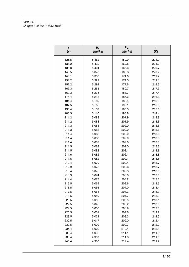
CPR 14EChapter 3 of the ‘Yellow Book’
3.105
126.5 5.462 159.9 221.7131.2 5.432 162.8 221.2135.8 5.404 165.6 220.7140.5 5.378 168.3 220.2145.1 5.353 171.0 219.7151.2 5.322 174.3 219.1157.2 5.292 177.6 218.5163.3 5.265 180.7 217.9169.3 5.238 183.7 217.4175.4 5.213 186.6 216.8181.4 5.189 189.4 216.3187.5 5.166 192.1 215.8195.4 5.137 195.5 215.1203.3 5.110 198.8 214.4211.2 5.083 201.9 213.8211.2 5.083 201.9 213.8211.3 5.083 202.0 213.8211.3 5.083 202.0 213.8211.4 5.083 202.0 213.8211.4 5.083 202.0 213.8211.4 5.082 202.0 213.8211.5 5.082 202.0 213.8211.5 5.082 202.1 213.8211.6 5.082 202.1 213.8211.6 5.082 202.1 213.8212.4 5.079 202.4 213.7212.9 5.078 202.6 213.7213.4 5.076 202.8 213.6213.9 5.074 203.0 213.6214.4 5.073 203.2 213.6215.5 5.069 203.6 213.5216.5 5.066 204.0 213.4217.5 5.063 204.3 213.3218.6 5.059 204.7 213.3220.5 5.052 205.5 213.1222.5 5.045 206.2 213.0224.5 5.038 206.9 212.8226.5 5.031 207.6 212.7228.5 5.024 208.3 212.5230.5 5.017 209.0 212.4232.5 5.009 209.7 212.2234.4 5.002 210.4 212.1236.4 4.995 211.1 211.9238.4 4.987 211.8 211.8240.4 4.980 212.4 211.7
t(s)
Hc
J/(m2⋅s)
Ha
J/(m2⋅s)T
(K)

3.106
242.4 4.973 213.1 211.5244.4 4.965 213.8 211.4246.4 4.958 214.4 211.3248.3 4.951 215.0 211.1251.7 4.939 216.1 210.9255.1 4.927 217.2 210.7258.5 4.916 218.2 210.5261.8 4.904 219.2 210.3265.2 4.893 220.2 210.0268.6 4.882 221.2 209.8274.0 4.866 222.7 209.5279.4 4.850 224.2 209.2284.8 4.834 225.7 208.9290.2 4.820 227.1 208.6295.6 4.806 228.5 208.3300.9 4.793 229.8 208.0308.7 4.775 231.7 207.6316.4 4.757 233.5 207.2324.2 4.741 235.2 206.8331.9 4.726 236.8 206.4339.7 4.712 238.4 206.1347.4 4.698 240.0 205.7356.6 4.683 241.7 205.3365.8 4.668 243.4 205.0374.9 4.654 245.0 204.6384.1 4.641 246.5 204.2393.3 4.628 248.0 203.9402.5 4.616 249.4 203.6411.6 4.605 250.7 203.3426.4 4.587 252.7 202.8441.2 4.570 254.6 202.3455.9 4.554 256.4 201.9470.7 4.539 258.1 201.5485.5 4.525 259.7 201.2500.2 4.511 261.1 200.8515.0 4.498 262.5 200.5532.7 4.482 264.0 200.1550.5 4.467 265.4 199.8568.2 4.453 266.7 199.5585.9 4.439 267.9 199.2603.6 4.426 269.0 198.9621.4 4.412 270.1 198.6639.1 4.400 271.0 198.4653.6 4.389 271.7 198.2668.2 4.379 272.4 198.0
t(s)
Hc
J/(m2⋅s)
Ha
J/(m2⋅s)T
(K)
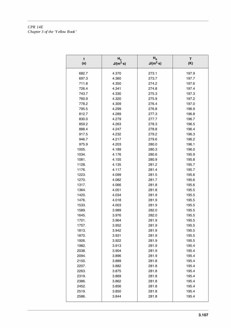
CPR 14EChapter 3 of the ‘Yellow Book’
3.107
682.7 4.370 273.1 197.9697.3 4.360 273.7 197.7711.8 4.350 274.2 197.6726.4 4.341 274.8 197.4743.7 4.330 275.3 197.3760.9 4.320 275.9 197.2778.2 4.309 276.4 197.0795.5 4.299 276.8 196.9812.7 4.289 277.3 196.8830.0 4.279 277.7 196.7859.2 4.263 278.3 196.5888.4 4.247 278.8 196.4917.5 4.232 279.2 196.3946.7 4.217 279.6 196.2975.9 4.203 280.0 196.1
1005. 4.189 280.3 196.01034. 4.176 280.6 195.91081. 4.155 280.9 195.81128. 4.135 281.2 195.71176. 4.117 281.4 195.71223. 4.099 281.5 195.61270. 4.082 281.7 195.61317. 4.066 281.8 195.61364. 4.051 281.8 195.51420. 4.034 281.9 195.51476. 4.018 281.9 195.51533. 4.003 281.9 195.51589. 3.989 282.0 195.51645. 3.976 282.0 195.51701. 3.964 281.9 195.51757. 3.952 281.9 195.51813. 3.942 281.9 195.51870. 3.931 281.9 195.51926. 3.922 281.9 195.51982. 3.913 281.9 195.42038. 3.904 281.9 195.42094. 3.896 281.9 195.42150. 3.889 281.8 195.42207. 3.882 281.8 195.42263. 3.875 281.8 195.42319. 3.869 281.8 195.42386. 3.862 281.8 195.42452. 3.856 281.8 195.42519. 3.850 281.8 195.42586. 3.844 281.8 195.4
t(s)
Hc
J/(m2⋅s)
Ha
J/(m2⋅s)T
(K)
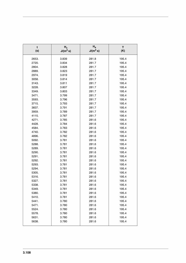
3.108
2653. 3.839 281.8 195.42720. 3.834 281.7 195.42804. 3.828 281.7 195.42889. 3.823 281.7 195.42974. 3.819 281.7 195.43058. 3.814 281.7 195.43143. 3.811 281.7 195.43228. 3.807 281.7 195.43349. 3.803 281.7 195.43471. 3.799 281.7 195.43593. 3.796 281.7 195.43715. 3.793 281.7 195.43837. 3.791 281.7 195.43959. 3.789 281.7 195.44115. 3.787 281.7 195.44271. 3.785 281.6 195.44428. 3.784 281.6 195.44584. 3.783 281.6 195.44740. 3.782 281.6 195.44896. 3.782 281.6 195.45092. 3.781 281.6 195.45288. 3.781 281.6 195.45289. 3.781 281.6 195.45290. 3.781 281.6 195.45291. 3.781 281.6 195.45292. 3.781 281.6 195.45293. 3.781 281.6 195.45294. 3.781 281.6 195.45305. 3.781 281.6 195.45316. 3.781 281.6 195.45327. 3.781 281.6 195.45338. 3.781 281.6 195.45349. 3.781 281.6 195.45380. 3.781 281.6 195.45410. 3.781 281.6 195.45441. 3.780 281.6 195.45471. 3.780 281.6 195.45524. 3.780 281.6 195.45578. 3.780 281.6 195.45631. 3.780 281.6 195.45638. 3.780 281.6 195.4
t(s)
Hc
J/(m2⋅s)
Ha
J/(m2⋅s)T
(K)
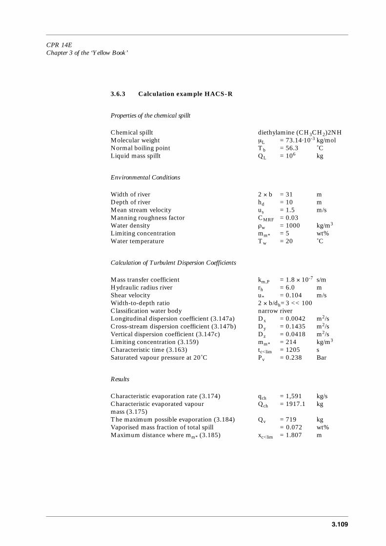
CPR 14EChapter 3 of the ‘Yellow Book’
3.109
3.6.3 Calculation example HACS-R
Properties of the chemical spillt
Chemical spillt diethylamine (CH3CH2)2NHMolecular weight µL = 73.14⋅10-3 kg/molNormal boiling point Tb = 56.3 ˚CLiquid mass spillt QL = 106 kg
Environmental Conditions
Width of river 2 × b = 31 mDepth of river hd = 10 mMean stream velocity us = 1.5 m/sManning roughness factor CMRF = 0.03Water density ρw = 1000 kg/m3
Limiting concentration mm* = 5 wt%Water temperature Tw = 20 ˚C
Calculation of Turbulent Dispersion Coefficients
Mass transfer coefficient km,P = 1.8 × 10⁻⁷ s/mHydraulic radius river rh = 6.0 mShear velocity u* = 0.104 m/sWidth-to-depth ratio 2 × b/dh=3 << 100 Classification water body narrow riverLongitudinal dispersion coefficient (3.147a) Dx = 0.0042 m2/sCross-stream dispersion coefficient (3.147b) Dy = 0.1435 m2/sVertical dispersion coefficient (3.147c) Dz = 0.0418 m2/sLimiting concentration (3.159) mm* = 214 kg/m3
Characteristic time (3.163) tc<lim = 1205 sSaturated vapour pressure at 20˚C Pv = 0.238 Bar
Results
Characteristic evaporation rate (3.174) qch = 1,591 kg/sCharacteristic evaporated vapour Qch = 1917.1 kgmass (3.175)The maximum possible evaporation (3.184) Qv = 719 kgVaporised mass fraction of total spill = 0.072 wt%Maximum distance where mm* (3.185) xc<lim = 1.807 m

3.110
3.6.4 Supplementary models
3.6.4.1 Evaporation of ammonia on a dry sandy subsoil
The model has been explained in paragraph 3.5.3.1.
Input
Chemical spilt ammonia (NH3)Total liquid mass released in the bund QL = 1000 kgBund area A = 100 m2
Initial temperature subsoil Ts,0 = 288.15 K
Physical properties
Normal boiling point Tb = 239.72 KHeat of vaporisation at boiling point Lv(Tb) = 1.209⋅106 J/kgtable 3.5:Thermal diffusivity (dry) sandy subsoil as,s = 2⋅10-7 m2/sThermal conductivity (dry) sandy subsoil λs,s = 0.3 J/(s⋅m⋅K)
Output
Heat flux conducting into the pool after 20 s Hc = 3.28⋅103 J/(m2⋅s)Vaporisation rate after 20 s qv = 2.71 kg/sTotal amount of vapour evolved after 20 s Qv = 108 kg
Procedure
The heat flux at time t = 20 s, from sandy subsoil can be estimated by equation(3.120). The momentaneous vaporisation rate can be estimated by equation(3.122a).The total amount of vapour evolved after 20 seconds can be estimated by equation(3.122b), which can not be more than the total mass of liquid ammonia mass releasedin the bund.
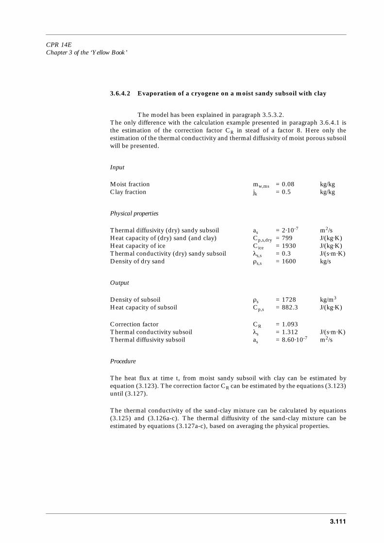
CPR 14EChapter 3 of the ‘Yellow Book’
3.111
3.6.4.2 Evaporation of a cryogene on a moist sandy subsoil with clay
The model has been explained in paragraph 3.5.3.2. The only difference with the calculation example presented in paragraph 3.6.4.1 isthe estimation of the correction factor CR in stead of a factor 8. Here only theestimation of the thermal conductivity and thermal diffusivity of moist porous subsoilwill be presented.
Input
Moist fraction mw,ms = 0.08 kg/kgClay fraction jk = 0.5 kg/kg
Physical properties
Thermal diffusivity (dry) sandy subsoil as = 2⋅10-7 m2/sHeat capacity of (dry) sand (and clay) Cp,s,dry = 799 J/(kg⋅K)Heat capacity of ice Cice = 1930 J/(kg⋅K)Thermal conductivity (dry) sandy subsoil λs,s = 0.3 J/(s⋅m⋅K)Density of dry sand ρs,s = 1600 kg/s
Output
Density of subsoil ρs = 1728 kg/m3
Heat capacity of subsoil Cp,s = 882.3 J/(kg⋅K)
Correction factor CR = 1.093Thermal conductivity subsoil λs = 1.312 J/(s⋅m⋅K)Thermal diffusivity subsoil as = 8.60⋅10-7 m2/s
Procedure
The heat flux at time t, from moist sandy subsoil with clay can be estimated byequation (3.123). The correction factor CR can be estimated by the equations (3.123)until (3.127).
The thermal conductivity of the sand-clay mixture can be calculated by equations(3.125) and (3.126a-c). The thermal diffusivity of the sand-clay mixture can beestimated by equations (3.127a-c), based on averaging the physical properties.
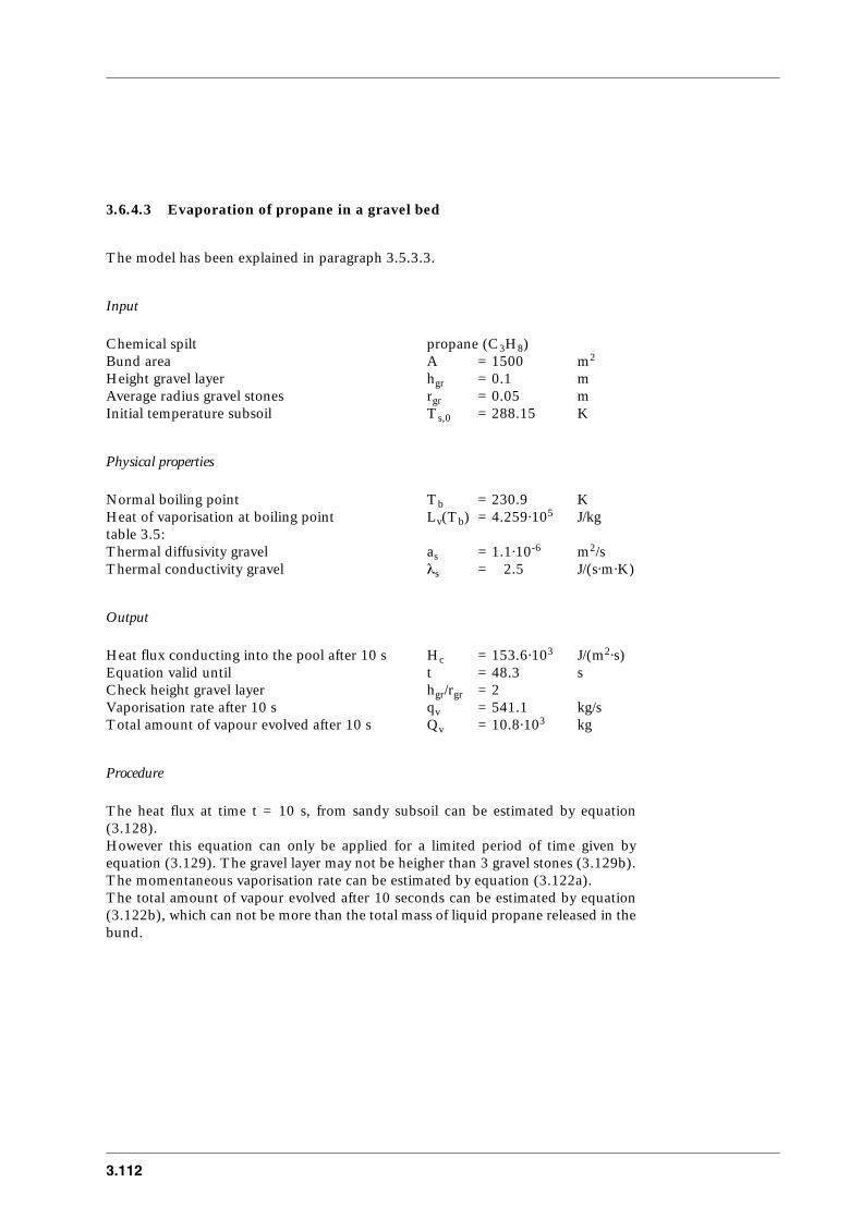
3.112
3.6.4.3 Evaporation of propane in a gravel bed
The model has been explained in paragraph 3.5.3.3.
Input
Chemical spilt propane (C3H8)Bund area A = 1500 m2
Height gravel layer hgr = 0.1 mAverage radius gravel stones rgr = 0.05 mInitial temperature subsoil Ts,0 = 288.15 K
Physical properties
Normal boiling point Tb = 230.9 KHeat of vaporisation at boiling point Lv(Tb) = 4.259⋅105 J/kgtable 3.5:Thermal diffusivity gravel as = 1.1⋅10-6 m2/sThermal conductivity gravel λs = 2.5 J/(s⋅m⋅K)
Output
Heat flux conducting into the pool after 10 s Hc = 153.6⋅103 J/(m2⋅s)Equation valid until t = 48.3 sCheck height gravel layer hgr/rgr = 2Vaporisation rate after 10 s qv = 541.1 kg/sTotal amount of vapour evolved after 10 s Qv = 10.8⋅103 kg
Procedure
The heat flux at time t = 10 s, from sandy subsoil can be estimated by equation(3.128).However this equation can only be applied for a limited period of time given byequation (3.129). The gravel layer may not be heigher than 3 gravel stones (3.129b).The momentaneous vaporisation rate can be estimated by equation (3.122a).The total amount of vapour evolved after 10 seconds can be estimated by equation(3.122b), which can not be more than the total mass of liquid propane released in thebund.
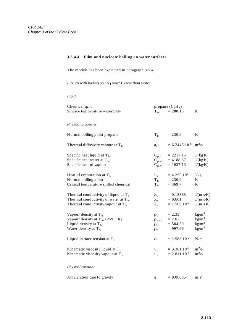
CPR 14EChapter 3 of the ‘Yellow Book’
3.113
3.6.4.4 Film and nucleate boiling on water surfaces
The models has been explained in paragraph 3.5.4.
Liquids with boiling points (much) lower than water
Input
Chemical spilt propane (C3H8)Surface temperature waterbody Tw = 288.15 K
Physical properties
Normal boiling point propane Tb = 230.9 K
Thermal diffusivity vapour at Tb av = 6.2445⋅10-6 m2/s
Specific heat liquid at Tb Cp,L = 2217.15 J/(kg⋅K)Specific heat water at Tw Cp,w = 4188.67 J/(kg⋅K)Specific heat of vapour Cp,V = 1037.13 J/(kg⋅K)
Heat of evaporation at Tb Lv = 4.259⋅106 J/kgNormal boiling point Tb = 230.9 KCritical temperature spilled chemical Tc = 369.7 K
Thermal conductivity of liquid at Tb λL = 0.13365 J/(m⋅s⋅K)Thermal conductivity of water at Tw λw = 0.601 J/(m⋅s⋅K)Thermal conductivity vapour at Tb λv = 1.509⋅10-2 J/(m⋅s⋅K)
Vapour density at Tb ρV = 2.33 kg/m3
Vapour density at Tav (259.5 K) ρV,av = 2.07 kg/m3
Liquid density at Tb ρL = 584.30 kg/m3
Water density at Tw ρw = 997.66 kg/m3
Liquid surface tension at Tb σ = 1.588⋅10-2 N/m
Kinematic viscosity liquid at Tb υL = 3.361⋅10-7 m2/sKinematic viscosity vapour at Tb υv = 2.811⋅10-6 m2/s
Physical constant
Acceleration due to gravity g = 9.80665 m/s2
3.114
Output
Maximum heat flux for nucleate boiling Hc,n,max = 3.21⋅106 J/(m2⋅s)(TL-Tw) corresponding with Hc,n,max ∆Tn,max = 12.9 KMinimum heat flux for film boiling Hc,f,min = 8.21⋅103 J/(m2⋅s)(TL-Tw) corresponding with Hc,f,min ∆Tf,min = 56.0 KActual heat flux Hc = 2.86⋅104 J/(m2⋅s)
Procedure
The heat flux for nucleate boiling can be estimated by equation (3.130), and can beexpressed as
Hc,n = 1510 × ∆T3 (J/(m2⋅s)) (3.130b)
The maximum heat flux for nucleate boiling Hc,n,max can be estimated by equation(3.131).From this two equations the temperature difference ∆Tn,max between the evaporatingliquid and the water surface for nucleate boiling, at which the heat flux is atmaximum, can be estimated.The minimum heat flux for film boiling Hc,f,min can be estimated by equations (3.132)and (3.133).The temperature difference ∆Tf,min between the evaporating liquid and the watersurface at which film boiling occurs can be estimated by equation (3.134).The heat flux during metastable boiling Hc,m could be calculated by means ofequation (3.130a), (3.135) and (3.136) in principle. However, the presenttemperature difference between water and propane ∆T = 57.3 K is larger than∆Tc,f,min. This means that the propane is fully film boiling. The actual heat flux Hchave been calculated by equation (3.107). The vaporisation mass rate could becalculated by equation (3.122).
Liquids with boiling points close to water
Input
Chemical spilt n-butane (C4H10)Surface temperature waterbody Tw = 288.15 K
Physical properties
Normal boiling point butane Tb = 272.7 KHeat capacity of water at Tw Cp,w = 4188.67 J/(kg⋅K)Thermal conductivity of water at Tw λw = 0.601 J/(m⋅s⋅K)Kinematic viscosity of water at Tw υw = 1.1168⋅10-6 m2/sThermal diffusivity of water at Tw aw = 1.4382⋅10-7 m2/sThermal expansivity of water at Tw αw = 2.0⋅10-4 1/K
Output
Heat flux Hc = 4.53⋅103 J/(m2⋅s)

CPR 14EChapter 3 of the ‘Yellow Book’
3.115
Procedure
The thermal diffusivity of water aw can be calculated by equation (3.6a).The (constant) heat flux can be estimated by equation (3.137).The vaporisation mass rate could be calculated by equation (3.122a).
3.6.4.5 Simple model non-boiling liquid in bund
The model has been explained in paragraph 3.5.5.2.
Input
Chemical spillt GasolineTotal mass released QL = 100000 kgInitial liquid temperature TL,0 = 288.15 KFixed pool surface A = 1500 m2
Initial temperature subsoil Ts,0 = 288.15 KWind velocity uw = 2 m/s
Isolation concrete:Thermal conductivity λs = 0.207 J/(m⋅s⋅K)Thermal diffusity as = 2.5⋅10-7 m2/s
Ambient temperature Ta = 288.15 KThermal conductivity air λa = 0.0257 J/(m⋅s⋅K)Prandtl number air Pra = 0.786Viscosity air ηa = 1.65⋅10-5 N⋅s/m2
Output
Evaporation rate at 600 sec qv = 10.25 kg/sTemperature of liquid at 600 sec TL = 273.06 K
Procedure1. The heat flux from the atmosphere: by convection Ha and solar radiated heat flux
Hrs, Hrl can be estimated by the methods addressed in paragraph 3.2.2.2. The unstationary heat flux from the ground Hc can be estimated by equations
(3.145a) and (3.145b).3. The vaporisation rate qv can be estimated by equations (3.141), (3.13), (3.21) and
(3.22) on the basis of the conditions of the pool at time t.4. The changing liquid pool temperature Tp can be determined by the equations
(3.142a) to (3.142d) and equation (3.143).5. The decreasing liquid height h can be determined by the equations (3.143a) and
(3.143b).
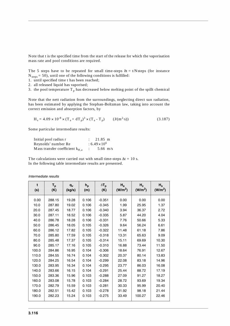
3.116
Note that t is the specified time from the start of the release for which the vaporisationmass rate and pool conditions are required.
The 5 steps have to be repeated for small time-steps δt = t/Nsteps (for instanceNsteps = 50), until one of the following conditions is fulfilled:1. until specified time t has been reached;2. all released liquid has vaporised;3. the pool temperature Tp has decreased below melting point of the spillt chemical
Note that the nett radiation from the surroundings, neglecting direct sun radiation,has been estimated by applying the Stephan-Boltzman law, taking into account thecorrect emission and absorption factors, by
Hs = 4.09 × 10⁻⁸ × (Ta + dTp)3 × (Ta - Tp) (J/(m2⋅s)) (3.187)
Some particular intermediate results:
Initial pool radius r : 21.85 mReynolds’ number Re : 6.49 × 10⁶ Mass transfer coefficient kH,a : 5.66 m/s
The calculations were carried out with small time-steps ∆t = 10 s.In the following table intermediate results are presented.
Intermediate results
t Tp qv hp δTp Ha Hc Hs
(s) (K) (kg/s) (m) (K) (W/m2) (W/m2) (W/m2)
0.00 288.15 19.28 0.106 -0.351 0.00 0.00 0.00 10.0 287.80 19.02 0.106 -0.345 1.99 25.95 1.37 20.0 287.45 18.77 0.106 -0.340 3.94 36.37 2.72 30.0 287.11 18.52 0.106 -0.335 5.87 44.20 4.04 40.0 286.78 18.28 0.106 -0.331 7.76 50.66 5.33 50.0 286.45 18.05 0.105 -0.326 9.64 56.24 6.61 60.0 286.12 17.82 0.105 -0.322 11.48 61.18 7.86 70.0 285.80 17.59 0.105 -0.318 13.31 65.63 9.09 80.0 285.48 17.37 0.105 -0.314 15.11 69.69 10.30 90.0 285.17 17.16 0.105 -0.310 16.88 73.44 11.50100.0 284.86 16.95 0.104 -0.306 18.64 76.91 12.67110.0 284.55 16.74 0.104 -0.302 20.37 80.14 13.83120.0 284.25 16.54 0.104 -0.299 22.08 83.18 14.96130.0 283.95 16.34 0.104 -0.295 23.77 86.03 16.08140.0 283.66 16.15 0.104 -0.291 25.44 88.72 17.19150.0 283.36 15.96 0.103 -0.288 27.09 91.27 18.27160.0 283.08 15.78 0.103 -0.284 28.72 93.69 19.34170.0 282.79 15.59 0.103 -0.281 30.33 95.99 20.40180.0 282.51 15.42 0.103 -0.278 31.92 98.18 21.44190.0 282.23 15.24 0.103 -0.275 33.49 100.27 22.46
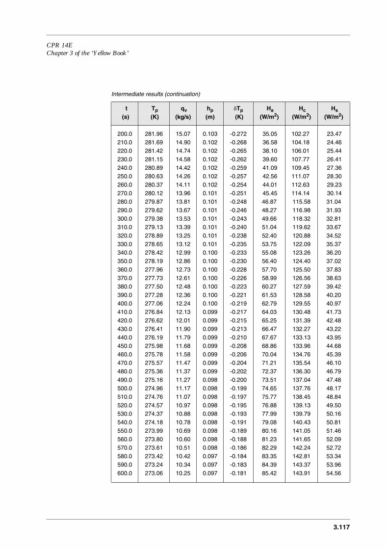
CPR 14EChapter 3 of the ‘Yellow Book’
3.117
200.0 281.96 15.07 0.103 -0.272 35.05 102.27 23.47210.0 281.69 14.90 0.102 -0.268 36.58 104.18 24.46220.0 281.42 14.74 0.102 -0.265 38.10 106.01 25.44230.0 281.15 14.58 0.102 -0.262 39.60 107.77 26.41240.0 280.89 14.42 0.102 -0.259 41.09 109.45 27.36250.0 280.63 14.26 0.102 -0.257 42.56 111.07 28.30260.0 280.37 14.11 0.102 -0.254 44.01 112.63 29.23270.0 280.12 13.96 0.101 -0.251 45.45 114.14 30.14280.0 279.87 13.81 0.101 -0.248 46.87 115.58 31.04290.0 279.62 13.67 0.101 -0.246 48.27 116.98 31.93300.0 279.38 13.53 0.101 -0.243 49.66 118.32 32.81310.0 279.13 13.39 0.101 -0.240 51.04 119.62 33.67320.0 278.89 13.25 0.101 -0.238 52.40 120.88 34.52330.0 278.65 13.12 0.101 -0.235 53.75 122.09 35.37340.0 278.42 12.99 0.100 -0.233 55.08 123.26 36.20350.0 278.19 12.86 0.100 -0.230 56.40 124.40 37.02360.0 277.96 12.73 0.100 -0.228 57.70 125.50 37.83370.0 277.73 12.61 0.100 -0.226 58.99 126.56 38.63380.0 277.50 12.48 0.100 -0.223 60.27 127.59 39.42390.0 277.28 12.36 0.100 -0.221 61.53 128.58 40.20400.0 277.06 12.24 0.100 -0.219 62.79 129.55 40.97410.0 276.84 12.13 0.099 -0.217 64.03 130.48 41.73420.0 276.62 12.01 0.099 -0.215 65.25 131.39 42.48430.0 276.41 11.90 0.099 -0.213 66.47 132.27 43.22440.0 276.19 11.79 0.099 -0.210 67.67 133.13 43.95450.0 275.98 11.68 0.099 -0.208 68.86 133.96 44.68460.0 275.78 11.58 0.099 -0.206 70.04 134.76 45.39470.0 275.57 11.47 0.099 -0.204 71.21 135.54 46.10480.0 275.36 11.37 0.099 -0.202 72.37 136.30 46.79490.0 275.16 11.27 0.098 -0.200 73.51 137.04 47.48500.0 274.96 11.17 0.098 -0.199 74.65 137.76 48.17510.0 274.76 11.07 0.098 -0.197 75.77 138.45 48.84520.0 274.57 10.97 0.098 -0.195 76.88 139.13 49.50530.0 274.37 10.88 0.098 -0.193 77.99 139.79 50.16540.0 274.18 10.78 0.098 -0.191 79.08 140.43 50.81550.0 273.99 10.69 0.098 -0.189 80.16 141.05 51.46560.0 273.80 10.60 0.098 -0.188 81.23 141.65 52.09570.0 273.61 10.51 0.098 -0.186 82.29 142.24 52.72580.0 273.42 10.42 0.097 -0.184 83.35 142.81 53.34590.0 273.24 10.34 0.097 -0.183 84.39 143.37 53.96600.0 273.06 10.25 0.097 -0.181 85.42 143.91 54.56
Intermediate results (continuation)
t Tp qv hp δTp Ha Hc Hs
(s) (K) (kg/s) (m) (K) (W/m2) (W/m2) (W/m2)

3.118

CPR 14EChapter 3 of the ‘Yellow Book’
3.119
3.7 Interfacing to other models
3.7.1 Introduction to section 3.7
The results from model predictions in this chapter ‘Pool Evaporation’ maybe used for further calculations as input for subsequent physical effect models,described in:
chapter 4 ‘Vapour Cloud Dispersion’, and chapter 6 ‘Heat flux from fires’.
The models in this chapter ‘Pool Evaporation’ may act as a source term model toprovide (quantitative) information about:– the amount of material entering the atmosphere by evaporation;– the dimensions of liquid pool;– the thermodynamic state of the evaporating liquids, such as concentrations,
temperature, and pressure.
Vapour cloud dispersion will occur when vapours are entering the atmosphere. Thepool evaporation models are able to determine the amount of vapour entering theatmosphere and the dimensions of the source.
On the other hand, the results from model predictions in chapter ‘Outflow and SprayRelease’ may provide the required input for pool evaporation models.
Interfacing to the relevant models in chapter 2 ‘Outflow and Spray Release’ andchapter 4 ‘Vapour Cloud Dispersion’ will be addressed in the following paragraphs.
Pool fires may occur after the ignition of a (spreading or shrinking) liquid pool.Models in this chapter ‘Pool evaporation’ can be addressed to estimate the initialdimensions of the pool before ignition. Interfacing to the relevant models in chapter6 ‘Heat flux from fires’ will be treated there.
Vapour cloud explosion can only occur after dispersion of flammable material in theatmosphere. After having estimated the characteristics of the evaporating liquid pool,models in chapter 4 ‘Vapour Cloud Dispersion’ have to be addressed first.
3.7.2 Outflow and Spray Release
3.7.2.1 Introduction
There are two ways by which liquid released from its containment can fallonto the ground or onto the water surface:1. rain out from airborne droplets may occur in case of a two-phase release;2. the liquid jet flows or falls directly onto the ground in case of a release of a ‘non-
boiling’ liquid.

3.120
3.7.2.2 Spray Release
3.7.2.2.1 Interfacing of spray release model for finite duration release of pressurised liquified gases
The mass flow rate of droplets falling onto the ground or onto the watersurface can be obtained from equation (2.161) in section 2.5.3.7
qd = qS - qnett,air (kg/s) (3.188a)
qd = mass rate of spray deposition [kg/s]qnett,air = mass flow rate remaining airborne [kg/s]qS = liquid source discharge rate [kg/s]
The distance from the source where the droplets will fall onto the ground or onto thewater surface will be less
x(t0) = uf × t0 (3.188b)
where t0, the time needed by a droplet to fall onto the ground or onto the watersurface, following from equation (2.160), and uf is the jet velocity after flashing,following from equation (2.149) This method provides an upper limit of x(t0) as inpractice the horizontal velocity will decrease due to resistance of the ambient air whenthe droplets fall.
3.7.2.2.2 Interfacing of spray release model for instantaneous release of pressurised liquified gases
The fraction of the release that will be deposited onto the ground or ontothe water surface follows from equation (2.183) in section 2.5.3.8.
Qd = Q - Qnett,air (kg) (3.189)
Qd = mass deposited spray [kg]Qnett,air = mass remaining airborne spray [kg]
The chemical will be deposited onto the ground or onto the water surface in the directvicinity of the two-phase release.
3.7.2.3 Liquid release
The interfacing of models predicting the (finite) mass flow rate isstraightforward. The (time-dependent) mass flow rate predicted by the models inparagraph 2.5.4 can be used without modification.

CPR 14EChapter 3 of the ‘Yellow Book’
3.121
For instantaneous liquid releases the total mass released provides sufficientinformation for the pool evaporation models.
3.7.3 Vapour cloud dispersion
3.7.3.1 Introduction
The predicted liquid pool evaporation rate qv will vary in time. For theatmospheric dispersion models requiring a (semi-)continuous source strength, thesame averaging method as described in paragraph 2.7.2.1 can be applied.
Both SLAB and GPM require dimensions of the source. By an integration over timeGPM can cope with varying source dimensions in principle. However, for SLABthese dimensions have to be constant. Note that in general the dimensions of the evaporating pool become less important ata greater distance from the pool, but are important at smaller distances.
For liquid releases within bunds, the dimensions of the bund can be used as sourcediameter, as the time for the pool to reach its maximum diameter is relatively short.
For durations after the initially spreading pool has reached its maximum diameter,the maximum pool diameter can be used as vapour source diameter for estimating themaximum concentration.
For spreading pools the matter is more complicated.Using the maximum dimensions of the spreading pool for the predictions of theatmospheric concentration at any time, would lead to underpredictions for neutralgases. Also the average pool diameter would underestimate the concentrations forshort durations after the start of the liquid release.Neglecting the pool dimensions as such, but not the (increasing) evaporation rate,would lead to overpredictions regarding the wind axis.Physically the concentration at the source can never be higher than the maximumconcentration based on the partial vapour pressure at the pool surface
ci,max < P˚(Ts) × µi/(R × Ts) (kg/m3) (3.190)
whereci,max = maximum concentration vapour [kg/m3]P˚ = vapour pressure as function temperature [N/m2]R = gas constant [J/(mol⋅K)]Ts = surface tempe rature pool [K]µi = mol mass vapour [kg/mol]
The diameter of the source might have an effect on the way heavy gas dispersionmodels predict the dispersion in the initial stage, where gravity slumping plays a role.Therefore, a smaller source diameter might lead to underpredictions under specificcircumstances.
3.122
Altogether we suggest to use the time-averaged pool diameter for the prediction of themaximum atmospheric concentrations at the wind axis during the spreading of thepool.
When estimating the concentration as a function of time, the travelling time t = x/uaof the vapour must be taken into account when switching the diameter of the liquidpool from the time-averaged pool diameter to the maximum (final) pool diameter.
3.7.3.2 Gaussian Plume Model
The Gaussian plume model (GPM, see section 4.5.3) can be applied if theevaporation results in neutrally or positively buoyant cloud.The input for the Gaussian Plume Model can be limited to the evaporation rate q in(4.51) and the dimensions of the pool by and bx.
3.7.3.3 The dense gas model of Britter and McQuaid
If the density after evaporation ρj > ρa, a dense gas dispersion model isneeded. The simplest model is the continuous release model by Britter and McQuaid,see section 4.5.5.1. Input of this model is volume flow rate vo. The volume flow ratevo can be calculated by
vo = qS/ρo (m3/s) (3.191)
with
ρV,0 = Pa × µi/(R × Ts) (kg/m3) (3.192)
wherePa = ambient atmospheric pressure [N/m2]qS = evaporation rate [kg/s]v0 = volume flow rate [m/s]ρV,0 = vapour density at the source [kg/m3]
3.7.3.4 SLAB model
Another dense gas dispersion model, SLAB, is described in section 4.5.5.2. The source conditions are using the SLAB notations (see e.g. Table 4.21):– Temperature of the source material TS: surface temperature liquid pool Ts.– Vaporisation flow rate of the source QS: qS.– Area of the source AS: appropriate pool area.
For this case the pool evaporation option should be applied, i.e. IDSPL=1
CPR 14EChapter 3 of the ‘Yellow Book’
3.123
3.8 Discussion
3.8.1 Introduction to section 3.8
In this section some general considerations on the models related to poolevaporation presented in this chapter are given and gaps in the description of poolevaporation are indicated.
3.8.2 General remarks
This chapter presents supplementary models for the evaporation inpermeable subsoil and different boiling regimes.A weakness of this chapter is that the supplementary models were not integrated intothe more general GASP model.To avoid inconsistencies and unforeseen numerical problems, the GASP model hasbeen copied unchanged, and it follows the original publications, although in ouropinion some sub-models are not optimal.
Models for pool evaporation from porous media are not well developed or based onlimited experimental data.No sufficient data are available in literature to enable a proper description of moistporous subsoil for the range (0 < mw,ms < 0.08).
The evidence that no substantial ice crust will be formed in case of a spill of cryogenon water, is not too strong.Limited information could be presented about chemicals that react with water, likeammonia and phosgene. The fraction of instantaneously spilt liquid ammonia onwater that is supposed to evolve from the water surface directly, is a rough estimatebased on limited evidence.No model for boiling liquids heavier than water, like chlorine, has been incorporatedinto this chapter.
3.8.3 Gasp
The GASP model describes pool evaporation of spreading boiling orvolatile liquids on land or floating on water.It is based on improved understanding of spreading phenomena, described by the so-called 'shallow layer equations', and of vaporisation, and the model forces thetransition of boiling to non-boiling to be smooth.The model turned out to be unavoidably complex as the simultaneous spreading,evaporating and (time-dependent) heat transfer, taking all heat sources into account,is a complex problem to solve.
3.124
In the model the mass transfer model is based on the theoretical work of Brighton[Brighton,1987]. For practical situations it is advisable to use the correlationKawamura & MacKay, based on experiments carried out in the open.
The description of the boiling process in GASP has been simplified by neglecting themetastable boiling regime, and by applying a somewhat simplified approach byassuming film boiling or a constant heat transfer coefficient.In literature a lot of attention is given to nucleate boiling and film boiling. Manycommon industrial liquefied gases will boil in the metastable boiling regime. So, theevaporation should be based on the model for metastable boiling.
The GASP model can still be approved regarding the following topics: dens gasbehaviour of the vapour, effects of pool surface waves, the effects of sloping andporous subsoil and multi-component liquid pools [Webber,1990].
The GASP-model has to be computerised before any prediction can be made. In casethe spreading of the liquid pool can be ignored, as may be the case for instantaneousliquid releases in bunds, it is possible to use simple models to guess the order ofmagnitude of the evaporation rate, at least with some accuracy. These models shouldbe used with care. Some rules of the thumb for their applicability and validity havebeen given.
3.8.4 HACS-R
The HACS-R model is able to predict the evaporation of soluble volatilechemicals caused by an instantaneous release.It has been assumed that all of the liquid goes into solution. This assumption is validbecause it appears that the total vapour generated is a small fraction of the mass spilt.In reality the release of chemicals takes place over a finite period. Since even in thecase of an instantaneous spill, the mass of vapour evolved appears a small fraction ofthe mass spilt, the predictions can be safely regarded as the worst case for longduration spills.
3.8.5 Epilogue
The gaps in the modelling of pool evaporation indicated here, leave plentyof room for further scientific research.
CPR 14EChapter 3 of the ‘Yellow Book’
3.125
3.9 References
AIChE (1989)Chemical Process Quantitative Risk Analysis - guidelines for -, Center for Chemical Process Safety of the American Institute of Chemical Engineers, 1989.
Aloha (1988)Aloha - Areal Locations of Hazardous Atmospheres Version 4.0 - Technical Appendix, Nat. Oceanic & Atmospheric Administration, USA, 1988.
Beek (1975)W.J. Beek and K.M.K. Muttzall, Transport Phenomena, J. Wiley and Sons Ltd, 1975.
Blanken (1980)J.M. Blanken, Behavior of Ammonia in the Event of a Spillage, American Institute of Chemical Engineers, 1980.
Bolz (1972)R.E. Bolz and G.L.T. Tuve, CRC Handbook of tables for Applied Engineering Science, 2nd Edition, 1972.
Brighton (1987)P.W.M. Brighton, Evaporation from a Plane Liquid Surface into a Turbulent Boundary Layer, SRD/HSE-report R375, January 1987.
Brighton (1990)P.W.M. Brighton, Further verification of a theory for mass and heat transfer from evaporating pools, J. of Hazardous Materials, 23 ,1990) 215-234.
Cavanaugh (1994)T.A. Cavanaugh, J.H. Siegell, K.W. Steinberg, Simulation of vapor emissions from liquid spills, J. of Hazardous Materials, 38 ,1994) 41-63.
Chang (1982)H.R. Chang and R.C. Reid, Spreading-boiling model for instantaneous spiulls of liquefied petroleum gas (LPG) on water, J. of Hazardous Materials, 25 ,1982) 19-35.
Dharmavaram (1994)S. Dharmavaram, J.N. Tilton, R.J. Gardner, Fate and transport of ammonia spilt from a barge, J. of Hazardous Materials, 37 ,1994) 475-487.
Frie (1992)J.L. Frie, G.A. Page, V. Diaz, J.J. Kives, Evaporation of containes and uncontained spills of multicomponent nonideal solutions, 7th Int. Symp. on Loss Prevention and Safety Promotion in the Process Industries, Taormina Italy 4-8 May 1992.
Jones (1992)D. Jones, Nomenclature for hazard and risk assessment in the process industries, second edition 1992, Institution of chemical Engineeers U.K.
3.126
Kawamura and MacKay (1987)P.I. Kawamura and D. MacKay, The Evaporation of volatile liquids, J. of Hazardous Materials, 15 ,1987) 365-376.
Melhelm (1993)G.A. Melhelm, and P.A. Croce, Advanced Consequence Modelling Emission, Dispersion, Fires, and Explosions, second draft July, 1993, A.D. Little.
Mikesell (1991)J.L. Mikesell, A.C. Buckland, V. Diaz and J.J. Kives, Evaporation of Contained Spills of Multicomponent Non-ideal Solutions, presented at Int. Conf. and Workshop on Modelling and Mittigating the Consequences of Accidental Releases of hazardous materials, May 20-24 1991, New Orleans, USA.
Nievergeld (1978)P. Nievergeld, W.F.Salitatu, Reduction of gasoline evaporation by a partially coverage of the surface of the liquid pool, TNO-CTI-report 78-01601 ,1978).
Phelps (1992)P.J. Phelps, R. Jureidine, The computer modelling of tank spills and containment overflows, 7th Int. Symp. on Loss Prevention and Safety Promotion in the Process Industries, Taormina Italy 4-8 May 1992.
Prince (1981)A.J. Prince, A users manual to spill, SRD/HSE-report R210, July 1981.
Prince (1985)A.J. Prince, Details and results of spill experiments of cryogenic liquids onto land and water, SRD-report R324, April 1985.
Raj (1974)Ph. K. Raj et al, Assessment models in support of the hazard assessment handbook, NTIS, January 1974.
Raj (1981)Ph. K. Raj, Models for cryogenic liquid spill behavior on land and water, J. of Hazardous Materials, 5 ,1981) 111-130.
Raj (1987)Ph. K. Raj and A.J. Morris, Source Characterisation and Heavy Gas Dispersion Models for Reactive Chemicals, Report AFGL-TR-88-0003(I) for the USA Air Force Geophysics Laboratory, Dec. 1987.
Raj (1991)Ph. K. Raj, Chemical Release/Spill Source Models - A review, presented at Int. Conf. and Workshop on Modelling and Mittigating the Consequences of Accidental Releases of hazardous materials, May 20-24 1991, New Orleans, USA.
Shaw (1978)P. Shaw and F. Briscoe, Evaporation from spills of hazardous liquids on land and water, SRD/HSE-report R100, May 1978.

CPR 14EChapter 3 of the ‘Yellow Book’
3.127
Stramigioli (1992)C. Stramigioli, G. Spadoni, Vaporisation from multicomponent liquid spills,7th Int. Symp. on Loss Prevention and Safety Promotion in the Process Industries, Taormina Italy 4-8 May 1992.
Studer (1988)D.W. Studer, B.A. Cooper and L.C. Doelp, Vaporisation and Dispersion Modelling of Contained Refrigerated Liquid Spills, Plant/Operations Progress, Vol. 7, No. 2, April, 1988.
SuperChems 4.0Superchems - A detailed Consequence Modelling Package -, A.D. Little, Inc, Cambridge, Massachusetts, USA.
Takeno (1994)K. Takeno, T. Ichinose, Y. Hyodo, H. Nakamura, Evaporation rates of liquid hydrogen and liquid oxygen spilt onto the ground, J. Loss Prev. Process Ind, 1994, Vol 7., Number 5.
Technica (1994)Personal communications with DNV Technica London.
Webber (1986)D.M. Webber and P.W.M. Brighton, Similarity solutions for the spreading liquid pools, SRD/HSE-report R371, July 1986.
Webber and Brighton (1987)D.M. Webber and P.W.M. Brighton, An integral model of spreading vaporising pools, SRD/HSE-report R390, August 1987.
Webber (1987)D.M. Webber, Heat conduction under a spreading pool, SRD/HSE-report R421, October 1987.
Webber (1988)D.M. Webber, A model for the evaporation and boiling of liquid pools, SRD/HSE-report R404, February 1988.
Webber and Jones (1988)D.M. Webber and S.J. Jones, A model of spreading vaporising pools, paper presented at the Int. Conference Cloud Modelling 1988.
Webber (1990)D.M. Webber, Model for Pool Spreading and Vaporisation and its Implementation in the Computer Code GASP, SRD/HSE-report R507, September 1990.
Webber (Jan. 1991)D.M. Webber, Source terms, J. Loss Prev. Process Ind, 1991, Vol 4., January.
3.128
Webber (Apr. 1991)D.M. Webber, A model of steady discharge into a vaporising pools, SRD/HSE-report R493, April 1991.
Webster (1981)Websters’ Third New International Dictionary, 1981.
Wilkinson (1991)A. Wilkinson, Bund overtopping - the consequences following catastrophic failure of large volume liquid storage vessels, SRD/HSE-report R530, October 1991.
Woodward (1990)J.L. Woodward, A integrated model for discharge rate, pool spread, and dispersion from punctured vessels, J. Loss Prev. Process Ind., 1990, Vol 3, January.
WorldBank (1988)Technica, Ltd., Techniques for Assessing Industrial Hazards, World Bank technical paper number 55.
YellowBook (1988)Methods for the calculation of physical effects of the release of dangerous materials (liquids and gases) 2nd ed., 1988), publ. by (Dutch) Directorate General of Labour; English version ,1992).
Zumsteg (1991)F. Zumsteg anf T.K. Fannalöp, Experiments on the Evaporation of Liquefied Gas over Water, presented at Int. Conf. and Workshop on Modelling and Mittigating the Consequences of Accidental Releases of hazardous materials, May 20-24 1991, New Orleans, USA.

4.1
Chapter 4Vapour cloud dispersionE.A. Bakkum, N.J. Duijm

CPR 14EChapter 4 of the ‘Yellow Book’
4.3
Modifications to Chapter 4 (Vapour Cloud Dispersion)with respect to the first print (1997)
Numerous modifications were made concerning typographical errors. A list is givenbelow for the pages on which errors have been corrected.
Some figures in this chapter were poorly printed; viz. figures 4.5, 4.16 and 4.18 aswell as the scheme in section 4.5.1. These prints have been improved.
Equation (4.51) on page 4.70 is a general expression for a continuous release.
In section 4.5.3.3 the equations (4.60) and (4.61) describe short duration releasesinstead of semi-continuous releases.In equation (4.60b)
σ
x
(x) has been replaced by
σ
x
(u
a
t).Below equation (4.61c) a sentence has been added concerning linear interpolation on
σ
x
for values of x less than 50 m.In section 4.5.3.6 it has been added that the proposed simplifications will introduceconsiderable continuity problems in calculating the concentration.
In section 4.5.4.1 describing the free turbulent jet model, equation (4.71) has beenreplaced and (4.73) has been removed. Hence all subsequent equations in chapter 4have been renumbered.
The constant in equation (4.79) has been adjusted, as well as the empirical constantsC
u
and C
c
in table 4.10.
The dispersion parameters were changed into the values of the 2
nd
edition ofCPR14E.
In section 4.5.4.2 the equations (4.83) and (4.84) have been adjusted, as well as theconstants in equations (4.87) and (4.92).In equation (4.149) an ending bracket just before the division line has been added.
In section 4.6.3 concerning application of the Gaussian plume model, the exampleshave been updated.Now subsection 4.6.3.1 describes the calculation of a plume and subsection 4.6.3.2shows the calculation of explosive mass of an instantaneous puff.Hence table 4.14 and figures 4.19 up to and including 4.21 have been replaced.
In subsection 4.6.4.1 the example on the free jet model has been corrected and figure4.22 has been replaced.
Section 4.6.5 describes example calculations for four source term submodels in theSLAB model. Some errors in the SLAB model have been corrected. All calculationsare updated and figures 4.23 up till and including 4.25 are replaced, whereas figure4.27 has been added. Furthermore the values for the Concentration averaging timeand Stability class in table 4.23 have been adjusted.

4.4

CPR 14EChapter 4 of the ‘Yellow Book’
4.5
List of symbols Chapter 4
Α cross-flow area of cloud or plume (4.26) m2
b half-width radius of jet or plume (4.16) mbo source radius (section 4.3.5.1.) mbox, boy, boz source half dimensions in down-wind,
cross-wind and vertical direction,respectively (4.62) m
bx, by half-width of cloud in down-wind andcross-wind direction, respectively (4.114) m
by,m effective plume half-width includingmeandering (4.145) m
bz cloud height (4.23) m
C general constants, to be defined in the textc(...) concentration as a function of the parts per unit volume
terms between brackets (4.5) or kg m-3
co concentration at source (4.25) p. p. u. v. or kg m-3
cc concentration at jet, plume or cloudcentre-line (4.28) p. p. u. v. or kg m-3
cr, cg peak concentration at maximum plume heightand plume touch-down, respectively (4.85) p. p. u. v. or kg m-3
cmax maximum concentration (Section 4.3.5.1) p. p. u. v. or kg m-3
cmean time-averaged concentration (Section 4.3.5.1) p. p. u. v. or kg m-3
cp specific heat at constant pressure (4.1) J kg-1 K-1
cp,a ambient specific heat at constant pressure (4.115) J kg-1 K-1
clfl, cufl lower and upper flammability concentration,respectively (4.66) p. p. u. v. or kg m-3
d particle diameter (4.4) m
e albedo (4.37) -Egh ground heat (4.115) J m-1 s-1
Epc phase change energy (4.115) J m-1 s-1
f ( ) general function, to be defined in the text,of the terms between brackets
f Coriolis parameter (4.8) s-1
fx, fy, fz drag term in down-wind, cross-wind andvertical direction, respectively kg s-2
F buoyancy flux factor (4.20) m4 s-3
Fo buoyancy flux factor at source (4.21) m4 s-3
Fd dry deposition flux (4.5) kg m-2 s-1
Fn wet deposition flux (4.6) kg m-2 s-1

4.6
Fx(..), Fy(..), Fz(..) expressions which account for along-wind, lateral,and vertical dispersion, respectively (4.28) m-1
Fr Froude number (4.17) -
g acceleration of gravity (4.1) m s-2
g' effective gravity g.(ρ - ρa)/ρa (4.20) m s-2
go' effective gravity at source g.(ρo - ρa)/ρa(section 4.3.5.1.) m s-2
h height of plume or cloud centre-line (4.11) mhi mixing height (4.9) mhs source height (4.86) m∆hr final plume rise (4.84) m∆hB plume rise due to buoyancy (4.88) m∆hM plume rise due to momentum (4.92) m
H0 sensible heat flux (4.1) J m-2 s-1
Hr net radiation heat flux (4.37) J m-2 s-1
Hrs incoming solar radiation (4.36) J m-2 s-1
Hri isothermal net radiation heat flux (4.41) J m-2 s-1
Hg ground heat flux (4.39) J m-2 s-1
Hl latent heat flux (4.39) J m-2 s-1
∆H heat of condensation (4.144b) J kg-1
I rain intensity (4.6) mm per hour
K reaction coefficient (4.3) -ks transfer coefficient (4.45) -
L Monin-Obukhov length(stability parameter) (4.1) m
Ls constant mLb buoyancy length-scale (4.101) m
m mass fraction of concentration (4.107) kg kg-1
Mo momentum from source (4.17) kg m s-2
N cloud cover (4.36) -
p (partial) pressure (4.142) N m-2
pa atmospheric pressure (4.143) N m-2
ps saturation pressure (4.143) N m-2
q mass flow rate (4.11) kg s-1
Q released mass (4.52) kg
r radial distance (4.23) m

CPR 14EChapter 4 of the ‘Yellow Book’
4.7
R gas constant (4.142) J mol-1 K-1
s coordinate along jet or plumecentre-line (4.16) m
sl length-scale parameter (4.71) mslfl distance to LFL (4.80) msh maximum jet height (4.79) mss length of potential core (Table 4.10) mso distance between real source and
virtual source (Table 4.10) m
t time (4.12) stav averaging-time (4.15) stmin minimum averaging-time (4.131) stL integral time-scale of atmospheric
turbulence (4.13) sti integral time-scale of dispersion (4.54) str release duration (4.60) stpk time to peak concentration (4.155) s
T temperature (4.138) KTa ambient temperature
(at screen height, about 2 m) (4.1) KTr upper level ambient
temperature (50 m) (4.41) KTo ambient temperature at
roughness height (4.40) KTs surface or sea temperature (4.40) KTw wet bulb temperature
(at screen height) (4.45) K
T* turbulent temperature scale (4.34) K
u (down-wind) velocity ofdispersing material (4.18) m s-1
ua ambient wind velocity (4.11) m s-1
uc velocity at jet or plume centre-line (4.73) m s-1
uo velocity at source (4.17) m s-1
uy, uz lateral and vertical velocity of dispersingmaterial, respectively (4.18) m s-1
u* surface friction velocity (4.1) m s-1
vo initial volume flow rate (4.100) m3 s-1
ve entrainment term (4.159) m3 s-1
V cloud volume (4.25) m3
Vo initial volume (4.25) m3
ws sedimentation velocity (4.4) m s-1
wd deposition velocity (4.5) m s-1
we entrainment velocity (4.16) m s-1

4.8
we,t top entrainment velocity (4.23) m s-1
we,e edge entrainment velocity (4.23) m s-1
we,x down-wind entrainment velocity (4.161) m s-1
we,y cross-wind entrainment velocity (4.161) m s-1
wH effective heat transfer velocity (4.136) m s-1
x down-wind horizontal coordinate m
xb shape parameter (4.168) mxc down-wind distance to centre of
mass of cloud (4.156) mxlfl, xufl down-wind distance to lower and upper
flammability level, respectively (4.66) mxu upwind extension of a
dense plume (4.101) mxr distance to maximum plume rise (4.83) mxg distance to plume touch-down (4.86) mxv, xvy, xvz virtual distances to account for finite source
dimensions during evaluation of plume size(4.68) m
y cross-wind horizontal coordinate (4.2) mylfl, yufl cross-wind distance to lower and upper
flammability limit, respectively (4.65) myb shape parameter (4.147) m
z vertical (upward) coordinate (4.2) mzb shape parameter (4.147) mzo surface roughness length (4.7) mzs constant (4.47) mzlfl height to lower flammability limit (4.65) m
Greek symbols
α moisture availability constant (4.38) -αl vapour mass fraction coefficient (4.138) -
γ ratio of specific heat of air to latentheat of water divided by rate ofchange (derivative) of saturation specifichumidity with temperature (4.38) -
γl liquid mass fraction coefficient (4.138) -
Γd dry adiabatic lapse rate (4.33) 0.011 K m-1
κ von Karman constant (4.1) 0.4
Λ wash-out coefficient (4.6) s-1 per (mm per hour)
µa molar weight of dry air (4.108) kg mol-1
µs molar weight of dispersing material (4.108) kg mol-1

CPR 14EChapter 4 of the ‘Yellow Book’
4.9
µmoist molar weight of moist air (4.139) kg mol-1
ν kinematic viscosity (4.4) m2 s-1
ρ density (4.2) kg m-3
ρa ambient density (4.1) kg m-3
ρp density of particle (4.4) kg m-3
ρs density of dispersing material (4.141) kg m-3
σ Stefan Boltzmann constant (4.37) 5.67.10-8 W m-2 K-4
σx, σy, σz down-wind, cross-wind and verticaldispersion parameters of cloud (4.11) m
σyi dispersion parameter of instantaneousplume width (4.56) m
σv, σw standard deviation of turbulent velocitiesin cross-wind and vertical direction,respectively (4.13) m s-1
φ conserved quantity (4.18) arbitrary
ϕ earth’s latitude (4.8) ˚N
χ solar elevation (4.36) ˚
ψ earth’s longitude (appendix 1) ˚W
Ψ stability function (4.32) -
Ω earth’s rotational speed (4.8) 7.27 . 10-5 s-1
Note: the numbers between brackets refer to equations.

4.10
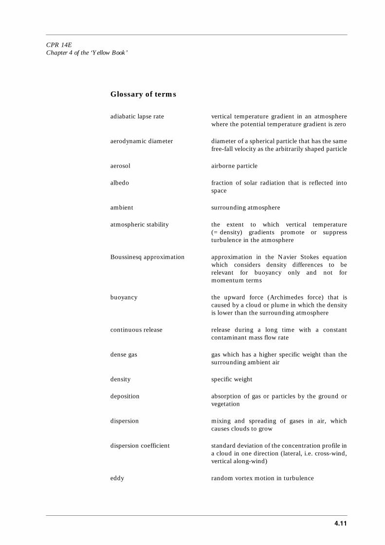
CPR 14EChapter 4 of the ‘Yellow Book’
4.11
Glossary of terms
adiabatic lapse rate vertical temperature gradient in an atmospherewhere the potential temperature gradient is zero
aerodynamic diameter diameter of a spherical particle that has the samefree-fall velocity as the arbitrarily shaped particle
aerosol airborne particle
albedo fraction of solar radiation that is reflected intospace
ambient surrounding atmosphere
atmospheric stability the extent to which vertical temperature(= density) gradients promote or suppressturbulence in the atmosphere
Boussinesq approximation approximation in the Navier Stokes equationwhich considers density differences to berelevant for buoyancy only and not formomentum terms
buoyancy the upward force (Archimedes force) that iscaused by a cloud or plume in which the densityis lower than the surrounding atmosphere
continuous release release during a long time with a constantcontaminant mass flow rate
dense gas gas which has a higher specific weight than thesurrounding ambient air
density specific weight
deposition absorption of gas or particles by the ground orvegetation
dispersion mixing and spreading of gases in air, whichcauses clouds to grow
dispersion coefficient standard deviation of the concentration profile ina cloud in one direction (lateral, i.e. cross-wind,vertical along-wind)
eddy random vortex motion in turbulence
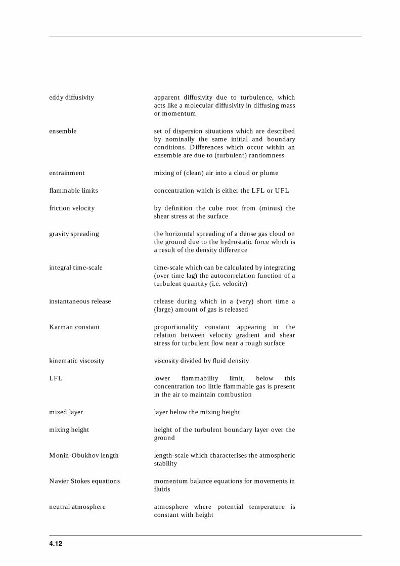
4.12
eddy diffusivity apparent diffusivity due to turbulence, whichacts like a molecular diffusivity in diffusing massor momentum
ensemble set of dispersion situations which are describedby nominally the same initial and boundaryconditions. Differences which occur within anensemble are due to (turbulent) randomness
entrainment mixing of (clean) air into a cloud or plume
flammable limits concentration which is either the LFL or UFL
friction velocity by definition the cube root from (minus) theshear stress at the surface
gravity spreading the horizontal spreading of a dense gas cloud onthe ground due to the hydrostatic force which isa result of the density difference
integral time-scale time-scale which can be calculated by integrating(over time lag) the autocorrelation function of aturbulent quantity (i.e. velocity)
instantaneous release release during which in a (very) short time a(large) amount of gas is released
Karman constant proportionality constant appearing in therelation between velocity gradient and shearstress for turbulent flow near a rough surface
kinematic viscosity viscosity divided by fluid density
LFL lower flammability limit, below thisconcentration too little flammable gas is presentin the air to maintain combustion
mixed layer layer below the mixing height
mixing height height of the turbulent boundary layer over theground
Monin-Obukhov length length-scale which characterises the atmosphericstability
Navier Stokes equations momentum balance equations for movements influids
neutral atmosphere atmosphere where potential temperature isconstant with height
CPR 14EChapter 4 of the ‘Yellow Book’
4.13
partial pressure fraction of total pressure due to the presence of agas; total pressure is the sum of all partialpressures of the gases present in a mixture
passive dispersion dispersion solely caused by atmosphericturbulence
phenomenological models models which present an empirical relationbetween initial and boundary conditions andobserved phenomena, without tempting todescribe the physical relationships
precipitation rain, snow, etc.
pure jet jet which is only driven by momentum
pure plume plume which is only driven by buoyancy
plume rise the ascent of a plume in the air due to verticalmomentum at the source or buoyancy
puff cloud spreading in all directions due to aninstantaneous release
regula falsi method to find a root of a function
roughness length artificial length-scale appearing in relationsdescribing the wind speed over a surface, andwhich characterises the roughness of the surface.Note the sizes of the elements causing theroughness can be more than ten times larger thanthe roughness length
saturation pressure pressure of a gas at saturated state. It depends ontemperature only; above the saturation pressurethe gas will condense
saturation specific humidity specific humidity of air with saturated watervapour, a function of temperature and, to a lesserextent, total pressure
sedimentation the deposition of particles on the ground due totheir free-fall velocity
4.14
semi-continuous release with a constant contaminant mass flowrate during a finite time
shear vertical velocity gradient
shear stress stress exerted by the wind on the ground surfacedue to friction
specific humidity humidity expressed as mass fraction of watervapour in air
stable atmosphere where potential temperatureincreases with height
still air air without detectable wind speed or direction
turbulence random motions in a fluid due to instabilities ofa large-scale flow
two-phase flow flow in which two phases are present, e.g. gas andliquid droplets or liquid with gas bubbles
UFL upper flammability limit, above thisconcentration too little oxygen is available tomaintain combustion
unstable atmosphere where potential temperaturedecreases with height
wash-out absorption of gas or particles in rain-drops fallingthrough a gas cloud or plume
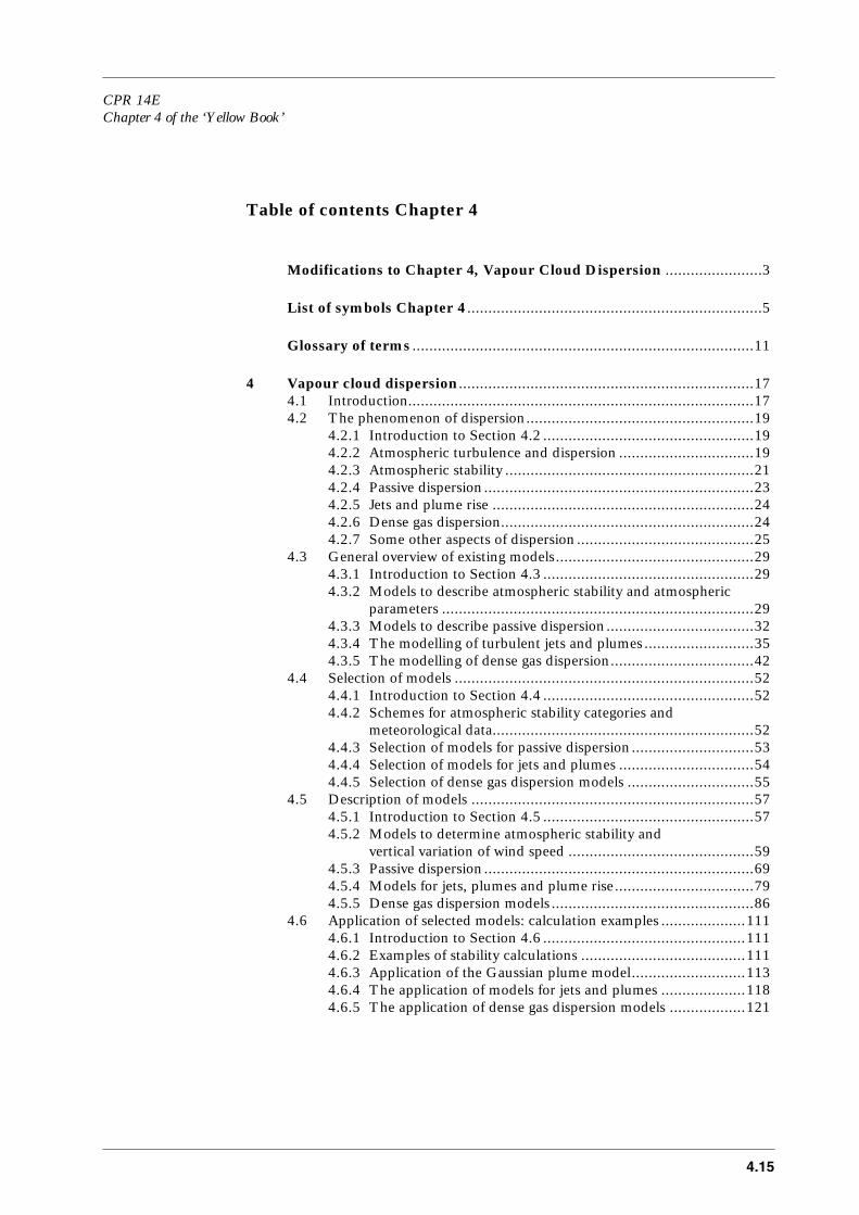
CPR 14EChapter 4 of the ‘Yellow Book’
4.15
Table of contents Chapter 4
Modifications to Chapter 4, Vapour Cloud Dispersion .......................3
List of symbols Chapter 4 ......................................................................5
Glossary of terms .................................................................................11
4 Vapour cloud dispersion......................................................................174.1 Introduction..................................................................................174.2 The phenomenon of dispersion......................................................19
4.2.1 Introduction to Section 4.2 ..................................................194.2.2 Atmospheric turbulence and dispersion ................................194.2.3 Atmospheric stability ...........................................................214.2.4 Passive dispersion ................................................................234.2.5 Jets and plume rise ..............................................................244.2.6 Dense gas dispersion............................................................244.2.7 Some other aspects of dispersion ..........................................25
4.3 General overview of existing models...............................................294.3.1 Introduction to Section 4.3 ..................................................294.3.2 Models to describe atmospheric stability and atmospheric
parameters ..........................................................................294.3.3 Models to describe passive dispersion...................................324.3.4 The modelling of turbulent jets and plumes ..........................354.3.5 The modelling of dense gas dispersion..................................42
4.4 Selection of models .......................................................................524.4.1 Introduction to Section 4.4 ..................................................524.4.2 Schemes for atmospheric stability categories and
meteorological data..............................................................524.4.3 Selection of models for passive dispersion .............................534.4.4 Selection of models for jets and plumes ................................544.4.5 Selection of dense gas dispersion models ..............................55
4.5 Description of models ...................................................................574.5.1 Introduction to Section 4.5 ..................................................574.5.2 Models to determine atmospheric stability and
vertical variation of wind speed ............................................594.5.3 Passive dispersion ................................................................694.5.4 Models for jets, plumes and plume rise.................................794.5.5 Dense gas dispersion models ................................................86
4.6 Application of selected models: calculation examples ....................1114.6.1 Introduction to Section 4.6 ................................................1114.6.2 Examples of stability calculations .......................................1114.6.3 Application of the Gaussian plume model...........................1134.6.4 The application of models for jets and plumes ....................1184.6.5 The application of dense gas dispersion models ..................121

4.16
4.7 Discussion.................................................................................. 1304.7.1 Introduction to Section 4.7 ............................................... 1304.7.2 Changes in atmospheric conditions.................................... 1304.7.3 Still air ............................................................................. 1304.7.4 Accuracy of the Gaussian plume model.............................. 1304.7.5 Dispersion over obstacles .................................................. 1314.7.6 Concentration fluctuations ................................................ 1314.7.7 Removal processes ............................................................ 132
4.8 Literature ................................................................................... 133
Appendix 4.1 A method for estimating the solar elevation
CPR 14EChapter 4 of the ‘Yellow Book’
4.17
4 Vapour cloud dispersion
4.1 Introduction
Hazardous material that is released in the atmosphere will be transportedand diluted by the wind. This chapter will provide models that enable the predictionof this transportation and dilution process for various release scenarios andconditions. The output of these models are concentrations (as a function of time) atany location surrounding the release (up to several kilometres). Moreover, the totalamount of hazardous material in a flammable vapour cloud between the upper andlower flammability limits will be predicted.
Dispersion will be restricted to dispersion within the atmospheric mixed layer in astationary state. This means that down-wind distances are restricted to typically10 km.
The input of the models described herein will be the results of the source term model,described in chapters 2 (Outflow and spray release) and 3 (Evaporation). Once thecloud, plume or jet interacts with the ambient air the dispersion processes describedin this chapter are to be applied.
The Sections 4.2 through 4.5 in this chapter will each address all of the four mainthemes of this chapter viz. atmospheric stability; passive dispersion; jets, plumes, andplume rise; and dense gas dispersion. However, each section will treat the topics witha different aim:
Section 4.2 provides the essential and basic understanding of the phenomena ofinterest. It provides information on atmospheric turbulence in general, and addressesshortly some topics beyond the main themes, viz. deposition, chemical reactions andobstacle effects.
Section 4.3 provides a general overview of the currently available methods andmodels for the main themes, which enable quantified analysis. It includes somephysical/mathematical background to models. The aim of the section is also toposition the models selected for detailed description among other existing models.
Section 4.4 presents the considerations which led to the selection of models which arefound to be acceptable for use and which are selected for detailed description.
Section 4.5 provides the detailed and complete description of the selected models.Whenever calculations or analyses have to be made, all necessary information can befound in this chapter. It is recommended to read the considerations presented insection 4.7 concerning validity and applicability of the models, before stating thecalculations.
Section 4.6 gives examples of the use of the models presented in section 4.5.

4.18
Finally, section 4.7 provides some information on general restrictions on the use ofmodels. It includes in some cases suggestions regarding methods to overcome theserestrictions or it recommends alternative approaches.
CPR 14EChapter 4 of the ‘Yellow Book’
4.19
4.2 The phenomenon of dispersion
4.2.1 Introduction to Section 4.2
This section provides the essential and basic understanding of thephenomenon of dispersion.– Section 4.2.2 introduces atmospheric turbulence and dispersion.– Section 4.2.3 explains atmospheric stability and the important parameters that
describe stability.– Section 4.2.4 describes the origin and effects of jets and plume rise.– Section 4.2.6 describes the basic phenomenon of dense gas dispersion.– Section 4.2.7 discusses some topics related to dispersion, viz. heat transfer,
chemical reaction, deposition and effects of obstacles.
4.2.2 Atmospheric turbulence and dispersion
The lower part of the atmosphere in which the releases take place is calledthe mixed layer. The height of the mixed layer (the mixing height) varies mostlybetween 200 and 2000 m. The wind flow in this mixed layer is almost alwaysturbulent, i.e. the movement of the air fluctuates continuously in velocity anddirection due to the presence of eddies. These turbulent eddies are very effective indispersing material through the air, a factor of at least 1000 more effective thanmolecular diffusion.
Turbulent flows are generally described in statistical terms, i.e. by a time-averagedmean velocity and a time-averaged standard deviation of velocity fluctuations aroundthis mean value.
Even for still-air, stable conditions turbulence is present due to temperaturedifferences in the atmosphere which cause movements of air.According to Hanna [1990], the standard deviations of horizontal turbulent velocitiesare not lower than 0.5 m/s (with a scatter of ± 0.3 m/s).
Turbulence is generated in two ways viz.:
1. Mechanically through the resistance of the earth’s surface on the wind. Thiscauses a decrease of wind speed to the surface (velocity gradient or shear). Thisshear causes turbulence due to flow instabilities, and a downward turbulent fluxof momentum to compensate the resistance force. The wind shear depends mainlyon the upper wind speed and the surface roughness.
2. Thermally due to heating of the surface (mainly by the sun). Hot patches of airnear the surface start to rise. This causes an upward turbulent flux of heat.
Without any generation of turbulence, turbulence will die due to viscous dissipation.Much more important in the atmosphere is the suppression of turbulence in steadily

4.20
stratified layers of air, i.e. in layers in which temperature increases upwards. Verticalmovements of air are suppressed.
An important aspect of atmospheric turbulence is the large range of sizes of theturbulent eddies, from several hundreds of metres diameter down to millimetres. Thedifferent sizes of eddies act differently in diffusing a puff of gas, see Figure 4.1.Turbulent eddies smaller than the size of the puff will uniformly disperse material andincrease the size of the puff (Figure 4.1a). Turbulent eddies much larger than thesize of the puff will only displace the puff without changing its size or geometry(Figure 4.1b). Eddies comparable to the size of the puff will change its geometry andincrease its contour (Figure 4.1c). These aspects are also relevant to theunderstanding of concentration fluctuations. At a certain position one will observefluctuations of concentrations due to meandering of the whole puff, and due todeformation of the puff. The concentration fluctuations are suppressed by smalleddies within the puff.As the puff grows, it is apparent that the number of eddies contributing to meanderingwill decrease, whereas ‘sub-puff’ eddies will contribute more and more to dispersion.The nature of turbulent dispersion changes during the life-time of the puff.
Figure 4.1 Dispersion of a puff of material under three turbulence conditions:(a) Puff embedded in a field in which the turbulent eddies are smaller than the puff.(b) Puff embedded in a field in which the turbulent eddies are larger than the puff.(c) Puff embedded in a field in which the turbulent eddies are comparable in size to the puff [Seinfeld, 1986]
(a)
(b)
(c)
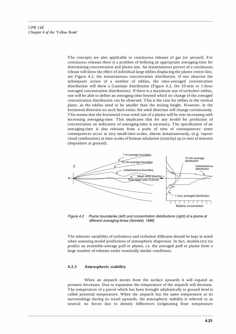
CPR 14EChapter 4 of the ‘Yellow Book’
4.21
The concepts are also applicable to continuous releases of gas (or aerosol). Forcontinuous releases there is a problem of defining an appropriate averaging-time fordetermining concentration and plume size. An instantaneous picture of a continuousrelease will show the effect of individual large eddies displacing the plume centre-line,see Figure 4.2, the instantaneous concentration distribution. If one observes thesubsequent action of a number of eddies, the time-averaged concentrationdistribution will show a Gaussian distribution (Figure 4.2, the 10-min or 1-houraveraged concentration distribution). If there is a maximum size of turbulent eddies,one will be able to define an averaging-time beyond which no change of the averagedconcentration distribution can be observed. This is the case for eddies in the verticalplane, as the eddies need to be smaller than the mixing height. However, in thehorizontal direction no such limit exists: the wind direction will change continuously.This means that the horizontal cross-wind size of a plume will be ever increasing withincreasing averaging-time. This implicates that for any model for prediction ofconcentration an indication of averaging-time is necessary. The specification of anaveraging-time is also relevant from a point of view of consequences: someconsequences occur at very small-time-scales, almost instantaneously, (e.g. vapourcloud combustion) at time-scales of human inhalation (toxicity) up to tens of minutes(deposition at ground).
Figure 4.2 Plume boundaries (left) and concentration distributions (right) of a plume at different averaging-times [Seinfeld, 1986]
The inherent variability of turbulence and turbulent diffusion should be kept in mindwhen assessing model predictions of atmospheric dispersion. In fact, models (try to)predict an ensemble-average puff or plume, i.e. the averaged puff or plume from alarge number of releases under nominally similar conditions.
4.2.3 Atmospheric stability
When an airpatch moves from the surface upwards it will expand aspressure decreases. Due to expansion the temperature of the airpatch will decrease.The temperature of a parcel which has been brought adiabatically to ground level iscalled potential temperature. When the airpatch has the same temperature as itssurroundings during its travel upwards, the atmospheric stability is referred to asneutral: no forces due to density differences (originating from temperature
y
x
1 hr average boundary
10 min average boundary
instantaneous boundary
Mean wind direction =Time mean axis of plume
Relative concentration
10 min averagedistribution
instantaneousdistribution
1 hour averaged distribution

4.22
differences) are exerted on the patch. If the temperature of the airpatch becomeslower than its surroundings, the atmosphere is stable; the airpatch is forceddownward. If on the contrary the temperature becomes higher than its surroundings,the atmosphere is unstable: the airpatch will accellerate upwards.
The vertical gradients of temperature are illustrated in Figure 4.3. From thermo-dynamics one calculates the dry adiabatic lapse rate to be -0.01 K/m. For saturatedair, the condensation of water vapour reduces the cooling of the air and the decreaseof temperature with height is less. This is the wet adiabatic lapse rate. For surfacetemperatures of about 290 K, the wet adiabatic lapse rate is about -0.005 K/m. (Dueto the change of saturation pressure, the difference between the dry and wet adiabaticlapse rate is larger at higher temperatures.) For temperature gradients between thetwo, the atmosphere is stable for dry air and unstable for saturated air. This regime iscalled conditionally unstable.
Figure 4.3 Temperature gradients and stability regimes in the atmosphere
During unstable conditions there is a heat flux from the surface upwards (this occursas the surface is heated by the sun). During stable condition the heat flux isdownwards (the surface is cooled at night by heat radiation to the sky). The stabilityof the mixed layer is determined by the ratio of turbulence generated by thetemperature gradient and the turbulence generated mechanically by wind shear at thesurface. This ratio can be expressed by a characteristic length-scale, the Monin-Obukhov length, which is defined as:
600
500
400
300
200
100
0283 284 285 286 287 288 289 290 291 292 293
temperature (K)
unstable
dry adiabaticlapse rate
wet adiabaticlapse rate
conditionallyunstable
stableheig
ht (
m)
L ρ
a c
p T
a u
*3
κ
gH
o
---------------------- –= (4.1)(m)
CPR 14EChapter 4 of the ‘Yellow Book’
4.23
The friction velocity u
*
is by definition the square root of the shear stress divided bythe density of air at the surface. H
o
is the sensible heat flux (see Section 4.5.2). In(4.1)
ρ
a
, c
p
, and T are the density, specific heat, and near surface temperature of theair, respectively.
κ
is the so-called Von Karman constant (
κ
≈
0.4) and g thegravitational acceleration.The Monin-Obukhov length provides a measure of stability of the mixed layer. L canbe interpreted as the height above the ground where turbulence generated by windshear equals the turbulence dissipated by the heat flux. In unstable conditions thereis not such an equilibrium, and this length is negative:
L > 0 stable (H
o
< 0)L < 0 unstable (H
o
> 0)L =
∞
neutral (H
o
= 0)
Table 4.1 Interpretation of the Monin-Obukhov length L with respect to atmospheric stability
Qualitative schemes to characterise stability are often used, e.g. the Pasquill scheme,which rates from class A (unstable) through D (neutral) to F (stable). Methods todetermine atmospheric stability and the relation with the Pasquill scheme aredescribed in Section 4.3.2.
4.2.4 Passive dispersion
Situations where the dispersion of a puff or cloud of material is governedsolely by the atmospheric turbulence are called passive dispersion. The state of theatmosphere is not changed by the presence of the material in the air.Assuming homogeneous turbulence and wind speed (i.e. the turbulence and windspeed are the same at all locations in the air) one can derive that the concentrationdistribution of an initially small puff of material becomes Gaussian in shape. Inpractice it appears that one observes a Gaussian distribution of concentration in verymany occasions. Many dispersion models are based on this Gaussian distribution;these will be discussed in more detail in Section 4.3.3.
L Stability condition
Small negative - 100 m < L < 0 Very unstableLarge negative - 10
5
m < L < - 100 m UnstableVery large (positive or negative) |L| > 10
5
m NeutralLarge positive 10 m < L < 10
5
m StableSmall positive 0 < L < 10 m Very stable

4.24
4.2.5 Jets and plume rise
4.2.5.1 Jets
Gases which are released with high velocity will cause jets. As long as thevelocity inside the jet is high compared to velocities in the ambient air, the extent andmixing in the jet is only affected by the properties of the jet itself.The velocity difference between the jet and the (assumed quiescent) surrounding airgenerates fine scale turbulence which causes the jet to spread sideways. The velocityin the jet reduces (about inversely proportional to the distance to the point of release).Finally the velocity will be reduced to such extent that passive dispersion takes over.
Models for free jets in still air and jets in cross-flow (wind) are discussed in Sections4.3.4.1 and 4.3.4.2 respectively.
4.2.5.2 Plume rise
Material released in the atmosphere may rise because:1. the material is less dense (buoyant) compared to the surrounding air and/or2. the material contains upward momentum.
Theoretically, in a neutrally or unstably stratified atmosphere, the material will riseindefinitely. However, due to mixing, the volume over which buoyancy and/ormomentum is distributed increases, and this causes the rate of plume rise to decreaserapidly. When vertical motion of the plume is of the same magnitude as the turbulentmotion of the plume one assumes the plume or puff to be at its final height.
In case the atmosphere is steadily stratified, there is a height at which the releasedmaterial, taking into account mixing during plume rise, will be in equilibrium with thedensity of the air at that height, which then is assumed to present the final plume rise.
After the plume has reached final plume rise, dispersion may be assumed to bepassive.For continuous releases from small source areas (stacks, vent pipes) a large numberof models for plume rise exist. These will be discussed in Section 4.3.4.2 to 4.3.4.3.
4.2.6 Dense gas dispersion
Releases of material denser than the ambient air introduce some specialeffects which affect the dispersion.The released material will descent to the surface and, once on the ground, spreadradially under influence of the gravitational forces. This self-induced flow produces ashallow cloud with increased horizontal extent. At the front of the so-called ‘gravity-current’ a head will develop with a strong vorticity (see Figure 4.4). This velocity fieldis deterministic in nature and will replace, for the duration of the gravity spreading,

CPR 14EChapter 4 of the ‘Yellow Book’
4.25
the random atmospheric turbulence. The self-induced flow will increase mixing,especially just behind the gravity head.
After gravity spreading has finished, the vertical variation of density in the cloud willcause a stable stratification in the cloud which reduces dispersion in vertical direction.Finally the effects of density will be dispersed and negligible and dispersion willbecome passive.
Dense gas dispersion models will be discussed in Section 4.3.5.
Figure 4.4 Gravity spreading of a dense gas cloud
4.2.7 Some other aspects of dispersion
In this section some aspects of dispersion are discussed that will not bediscussed separately or in detail in the remainder of this chapter. These are: heattransfer, chemical reactions, deposition, and obstacle effects.
4.2.7.1 Heat transfer and change of buoyancy
Often the total buoyancy in a cloud, either negative (dense cloud) orpositive, remains constant during the dispersion process. This is referred to by sayingbuoyancy is conserved.For an instantaneous release this can be expressed as:
Here,
ρ
(x,y,z) denotes the density in the cloud and
ρ
a
(z) denotes the density of theambient air at the same height.
head head
air
vortex
gravityspreading
ρ x,y,z( ) ρa z( )– dx dy dz ∫∫∫ cons ttan =
all space
(4.2)(kg)

4.26
However, some processes in the cloud may change the total buoyancy:
–
heat transfer from the surface to the cloud;
–
vaporisation of liquid aerosol in the cloud;
–
condensation and evaporation of water vapour aerosol in the cloud;
–
chemical reactions which change the number of moles and/or which areendothermic or exothermic.
Heat transfer from the surface is relevant to cold plumes, originating e.g. fromreleases of cryogenic gases. The warm surface heats the cold gas, which can changefrom negatively buoyant to positively buoyant, causing the cloud to lift from theground.Depending on the velocity of the cloud over the surface and the temperaturedifference, heat transfer is dominated by forced convection or by free convection. Forforced convection, the heat flux from the surface is about proportional to the frictionvelocity and the temperature difference. For free convection, the heat flux isindependent of velocity and about proportional to the temperature difference to thepower 4/3 rd.
Vaporisation of liquid aerosol, during releases of e.g. pressurised liquified gases, willcool down the air/gas mixture in the cloud, increasing its negative buoyancy.
The ambient air contains always some water vapour. For releases of cold material, thewater vapour mixed into the cloud may condensate, thereby increasing the buoyancy.At a later stage, the condensed water may well evaporate again, cooling down thecloud, but these effects often happen at a distance or travel time from the release,where density effects are no longer relevant.
If the released material reacts with components in the air during which the numberof molecules change, the total buoyancy is no longer conserved. If the number ofmolecules decreases, the cloud will become denser and vice versa. The heat producedor required by the chemical reaction will change the total buoyancy as is the case withcondensation or evaporation of water.
4.2.7.2 Chemical reactions
Chemical reactions will also convert the initialy released substance intoanother secondary substance. From a point of view of hazards one might be interestedin the primary substance or in the secondary.In general, a reaction of the form
A + B
→
C + D
is controlled by a reaction constant K which determines equilibrium between thesubstances A, B, C and D:
K A[ ] B[ ]
C[ ] D[ ]------------------ (K can be zero or infinite)= (4.3)(-)
CPR 14EChapter 4 of the ‘Yellow Book’
4.27
([A], [B], etc, denote concentrations of the substances A, B, etc.)
Local deviations from equilibrium are due to finite reaction rates and, relevant nearthe release, to concentration fluctuations inside the cloud.
4.2.7.3 Deposition
Material can be removed from the cloud by deposition of material on theground. One may discriminate the following deposition mechanisms:
–
sedimentation of aerosols;
–
dry deposition of gases and aerosols at the surface;
–
wet deposition by precipitation (rain, snow) of gases and aerosols from the cloud.
All particles in the air have a finite sedimentation velocity. The sedimentation velocityw
s
can be approximated by Stokes law:
Here d is the (aerodynamic) diameter of the particle and the specific density of theparticle,
ρ
a
the density of air, g is gravitational acceleration, and
ν
is the kinematicviscosity of air.In practice one may assume that the sedimentation velocity of particles smaller than10 diameter (w
s
< 0.02 m/s) is negligible, and that dispersion of these particles issimilar to dispersion of gas.
Dry deposition of aerosols and gases can be described as a deposition flux F
d
whichis the product of a deposition velocity w
d
and a concentration c at some referenceheight above the surface.
F
d
= w
d
c (kg m
-2
s
-1
) (4.5)
The deposition velocity is the inverse of the sum of three resistances; viz. anaerodynamic resistance dominated by turbulence and stability of the atmospherebetween the surface and the reference height; a resistance which is caused by the flowaround structures at the surface (surface induced resistance), dominated by thefriction velocity and surface roughness, and a surface resistance, which depends onthe properties of the substance (e.g. solubility in water) and the type of surface(vegetation).The aerodynamic resistance can change from about 1000 s/m (stable conditions,smooth surface and low wind speed) down to 3 (high-wind speed, rough surface).Typical values for the surface induced resistance are in the order of 10 s/m. Surfaceresistances can vary from order of 10 to more than 1000 s/m.
Wet deposition only occurs during precipitation, but it can be much moreeffective than dry deposition. Wet deposition can be described by a wash-out
ws1
18-----d2g
ρp
ρaν--------= (4.4)(m s-1)
ρp
µm
4.28
coefficient (s
-1
per mm precipitation per hour)
1)
and an intensity of precipitation I(mm/hour)
1)
. The wet deposition flux F
n
can be written as:
Here, c(z) is the concentration in the cloud. For aerosol is typically 4.10
-4
s
-1
fora precipitation of 1 mm per hour.
4.2.7.4 Obstacle effects
Dispersion over flat terrain with homogeneous roughness of which theindividual roughness elements are smaller than the height of the cloud is rather wellunderstood. The flow and dispersion around individual obstacles or arrays ofobstacles is difficult to describe and to quantify in a general way (for a number ofspecific situations approximate solutions have been found).Obstacle effects however are important. A rule of thumb to estimate when to accountfor obstacles is that the smaller value of height or width (in cross-wind direction) islarger than 0.5 to 1. times the local cloud height.Behind obstacles a so-called recirculation zone exists. This zone may extend to about10 times the obstacle height [Duijm and Webber, 1993]. Due to increased turbulencein the wake of the obstacle, the maximum groundlevel concentration down-wind ofthe recirculation is lower than in the absence of the obstacle. Nearer to obstacles nogeneral trend can be indicated: an increase of concentration is possible and increasesby a factor of 2 have been reported.
1)
Λ
and I are usually expressed in these non-SI units.
Λ
Fn ΛI c z( )dzsurface
cloudheight
∫= (4.6)(kg m-2 s-1)
ΛI
CPR 14EChapter 4 of the ‘Yellow Book’
4.29
4.3 General overview of existing models
4.3.1 Introduction to Section 4.3
Section 4.3 provides an overview of methods and models used fordispersion calculations. It presents alternative methods and provides shortdescriptions of the contents of the main types of models in a general way.In this section the following themes are discussed:
–
Section 4.3.2 presents atmospheric stability schemes and methods to predictcharacteristics of the atmosphere.
–
Section 4.3.3 presents passive dispersion models with emphasis on the Gaussianplume models.
–
Section 4.3.4 presents models for jets and plumes in still air and in ambient wind,and simple models for plume rise.
–
Section 4.3.5 presents various types of dense gas dispersion models.
4.3.2 Models to describe atmospheric stability and atmospheric parameters
4.3.2.1 Atmospheric stability classifications
All models used to describe or predict atmospheric dispersion needinformation about the stability of the atmosphere, mainly to define the rate at whichthe material is passively dispersed by atmospheric turbulence. This information canbe obtained through various methods:
–
Direct measurement of the intensity of wind direction fluctuations in lateral andvertical direction [Erbrink, 1991]. This method requires measurements which arenot routinely carried out. The link with alternative schemes (e.g. the Pasquillscheme, see below) is difficult. However, the results can be directly applied tocalculate the dispersion parameters (plume widths) for the Gaussian plumemodel.
–
Classification of horizontal wind direction traces as defined by Singer and Smith71953], the so-called Brookhaven Gustiness Classes, changing from Class A(unstable) to Class D (stable). It is not clear whether this scheme can representstability adequately over different types of terrain and different climates.
–
Classification of atmospheric stability from routine meteorological data, such asthe well-known Pasquill scheme [Pasquill and Smith, 1983] which is based onobservations of wind speed, cloud cover and time of day. The Pasquill scheme iscurrently the most applied scheme.
–
Direct measurement of friction velocity u
*
and Monin-Obukhov lenght L, whichprovides an unambiguous measure of stability in the lower part of the atmosphericboundary layer (see Section 4.2.2). These measurements are not routinely carriedout. The link to e.g. the Pasquill scheme can be made.

4.30
–
Calculation of friction velocity and Monin-Obukhov length from routinemeteorological data and terrain specification as by Holtslag, Nieuwstadt and VanUlden [Holtslag, 1984; van Ulden and Holtslag, 1985; Holtslag and Nieuwstadt,1986; Holtslag and de Bruin, 1987; Holtslag, 1987]. The link to the Pasquillscheme can be made.
Most widely-used dispersion models make use of the Pasquill stability categories(A-unstable to F-stable) and parametrisations of the local lateral and vertical plumewidth (
σ
y
and
σ
z
) corresponding to Pasquill-Gifford, Briggs, Smith, etc. (see e.g.Seinfeld [1986], pp 577).
However, better results can be obtained if the qualitative schemes are exchanged infavour of schemes using quantifications of physical parameters of the boundary layer(such as roughness length z
o
, heat flux H
o
, friction velocity u
*
, and Monin-Obukhovlength L).A complete scheme using routinely meteorological data has been developed byHoltslag, Nieuwstad and Van Ulden. The scheme is based on providing an estimateof the surface heat budget, i.e.:
sensible heat flux + latent heat flux + heat flux into the soil =
net radiation =
(1 - albedo) * solar radiation + incoming long wave radiation
- outgoing long wave radiation
The sensible heat flux determines the stability of the atmosphere. Holtslag’s schemeprovides methods of estimating all terms in the equation above based on routinelyavailable data and information of the local situation (e.g. surface roughness, albedoand solar elevation). Holtslag’s scheme is described in Section 4.5.2.
It is possible to link the Pasquill stability scheme to the Monin-Obukhov lengthdepending on local surface roughness by a graph proposed by Golder [1972]. Thismethod is included in Section 4.5.2 (see Figure 4.11).
The stability over extended water surfaces (seas) depends mainly on the temperaturedifferences between the air and the water. From the temperature difference one cancompute the sensible heat flux which, together with the friction velocity, determinesstability. Hsu [1992] developed a simple scheme (nomogram) to relate the stability interms of Monin-Obukhov length and Pasquill classes to the temperature differencebetween the water surface and the air and the wind speed, which are routinelyavailable data, see Section 4.5.2.4 and Figure 4.12.
CPR 14EChapter 4 of the ‘Yellow Book’
4.31
4.3.2.2 Other atmospheric characteristics
Almost all characteristics of the mixing layer can be expressed in terms ofstability parameters (friction velocity u* and Monin-Obukhov length L). Quantitiesrelevant to dispersion are:– vertical variation of wind speed; – vertical variation of standard deviations of turbulent velocities in cross-wind and
vertical direction (σv and σw respectively);– mixing height.
Variation of wind speedThe vertical variation of wind speed is often approximated by a power law.Alternatively, wind speed ua can be described by relations which follow fromsimilarity theory in the surface layer:
ua(z) = f(z/zo, z/L) (m s-1) (4.7)
Here f(z/zo, z/L) is an empirical function, u* the friction velocity and κ the VonKarman constant. This relation is adequate up to a height of about 100 m abovewhich the vertical variation of wind speed can be neglected. Well-known suggestionsfor the function f are from Businger and Dyer and Bradley and can be found in thetext books Pasquill and Smith [1983], Seinfeld [1986], Panofsky and Dutton [1984],and Stull [1988]. More details can be found in Section 4.5.2.
Turbulence parametersValues for standard deviations of turbulent velocities in the surface layer are providedby Panofsky and Dutton [1984]. Proposals for formulae describing the verticalvariation of these quantities can be found in Gryning et al. [1987], Seinfeld [1986]and Stull [1988]. More information is provided in Sections 4.4.2 and 4.5.2.
Mixing heightThe mixing height depends on:– height of inversion layers;– surface friction velocity;– Monin-Obukhov length;– latitude of position on earth.
The height of inversion layers is very often dominated by advection of large-scale airmasses in which these inversion layers are present. These have little relation with thelocal situation of the mixing layer at any given moment. In The Netherlands themixing height is dominated by these inversion layers about one third of the time. Thissituation will be different in other areas, depending on location on earth, proximity toseas and oceans, etc.
If no inversion layers are present, one might estimate the local mixing height from u*,L and the Coriolis parameter f, which is defined as:
f = 2 Ω sin ϕ (s-1) (4.8)
u*κ-----

4.32
with Ω the earth rotation (7.27 . 10-5 s-1) and φ the latitude of position on earth (about51˚ for The Netherlands).For purely neutral conditions, the mixing height can be calculated as (see e.g.Panofsky and Dutton, [1984]):
For stable conditions one may write for stationary conditions [Panofsky and Dutton,1984, Pasquill and Smith, 1983]:
No stationary solution exists for the mixing height in unstable conditions. The mixingheight at a certain time of day can be calculated from the vertical temperature profileat sunrise and the time integrated heat flux since sunrise.
Statistical information about mixing heights can also be estimated frommeteorological data. This information accounts for the effects of elevated inversions,but it can not be applied to all positions on earth. For calculations involving unstableconditions without information of time, this is the only applicable method.Suggestions for mixing height predictions, based on statistical meteorologicalinformation and formulae (4.9) and (4.10) above, are presented in Section 4.5.2.
4.3.3 Models to describe passive dispersion
Passive dispersion is governed by atmospheric turbulence. Atmosphericturbulence is determined by the stability of the atmosphere and the height above thesurface. Gryning et al. [1987] have defined scaling regions in the atmosphere(Figure 4.5).
Gaussian plume models have been used extensively for all regions mentioned inFigure 4.5. The basic expression for the Gaussian plume model for a continuousrelease is:
hi 0.2 u * f ⁄ = (4.9)(m)
hi 0.4u*
f----- L = (4.10)(m)
c x,y,z( )q
2π u a σ y σ z ------------------------ . exp y
2
2
σ
y
2
-------- –
. exp h z – ( ) 2
2
σ
y
2
----------------- –
= (4.11)(kg m -3 )

CPR 14EChapter 4 of the ‘Yellow Book’
4.33
Figure 4.5 The scaling regions of the atmospheric boundary layer shown as function of the dimensionless height z/h
i
, and the stability parameter h
i
/L. A detailed discussion can be found in Holtslag and Nieuwstadt [1986]. When used to determine dispersion regions, the dimensionless height is replaced by h/h
i
where h is the source height.
The equivalent expression for an instantaneous release is written as:
In (4.11) and (4.12) c(x,y,z) is the concentration at position x,y,z. Q and q are thetotal released mass and release rate, respectively. u
a
is the ambient velocity at whichthe plume or puff is advected by the wind.
σ
x
,
σ
y
, and
σ
z
are the so-called dispersionparameters in along-wind, cross-wind, and vertical direcion, respectively. The heightof the plume centre-line is denoted by h.For plumes near the ground or near the mixing height additional terms appear in(4.11) and (4.12) to account for ‘reflection’ of material against the surface or themixing height.
Within the framework of the Gaussian plume models, differences may appear in:
–
the choice of the plume averaged transport velocity u
a
: and
–
the choice of the dispersion parameters
σ
x
,
σ
y
, and
σ
z
.
In most applications of the Gaussian plume model the transport velocity is taken asthe wind speed at plume height h, with a minimum of h for surface releases.
Entrainment layer
Mixed layer Near neutralupper layer
z-less scaling layer
Intermittencylayer
Localscaling layer
Surface layerSurface layer
Freeconvectionlayer
1.2
0.8
zhi
0.1
0.01
-100 hi
L-10
unstable
-1
neutral
0 1 5 10hi
L
N.n
eu.u
p.la
yer
stable
c x,y,z,t( )Q
2π( )3/2σxσyσz
-------------------------------- . expx u
a .t– ( )
2
2
σ
x
2
----------------------- – . exp y
2
2
σ
y
2
-------- – .=
exp h z–( )2
2σz2
-----------------–
(4.12)(kg m-3)

4.34
With respect to the dispersion parameters
σ
x
,
σ
y
, and
σ
z
different approaches can befollowed, two of which are mentioned here. The fundamentals of the differentapproaches are discussed in Pasquill and Smith [1983].
The first approach is based on the statistical theory of dispersion in homogeneousturbulence. This leads to expressions in which the spread (i.e. the dispersionparameter) in any direction is proportional to the intensity of velocity fluctuations inthat direction times a function of travel time t and some integral time-scale of theturbulence t
L
:
σ
x
=
σ
u
f (t,t
L
);
σ
y
=
σ
v
f (t,t
L
);
σ
z
=
σ
w
f (t,t
L
) (m) (4.13)
Several proposals for the function f (t,t
L) for σy and σz have been suggested, see e.g.Pasquill and Smith [1983], Panofsky and Dutton [1984], Stern et al. [1984], andSeinfeld [1986]. The function as suggested by Draxler [Stern et al., 1984] for σy andσz is widely used.
The other approach is to provide fits to experimental data without a link to theoreticalconsiderations. This leads to expressions of the form:
σx = f (x); σy = f (x); σz = f (x) (m) (4.14)
Widely-used suggestions for the function f(x) for σy and σz are those of Pasquill-Gifford, M.E. Smith and Briggs [Pasquill and Smith, 1983; Stern et al., 1984;Panofsky and Dutton, 1984]. Seinfeld [1986] also includes the suggestions by Klugas incorporated in German guidelines for stack plume dispersion modelling.
Strictly speaking, the Gaussian plume model can not be used for description ofpassive dispersion in the surface layer because the vertical variations of wind speedand turbulence intensity in the surface layer cause the vertical concentrationdistribution to deviate from a normal distribution. Based on similarity theory and theconcept of eddy-diffusivity one is able to provide analytical solutions orapproximations for the vertical concentration distribution [Pasquill and Smith, 1983;Van Ulden, 1991, Gryning et al., 1987].
Little information is available on the along-wind dispersion parameter σx for (near)instantaneous releases. Not only turbulence in along-wind direction contributes tothe increase of σx, but also the vertical variation of wind speed contributes to anincrease of σx. Van Ulden [1991] provides a scheme for σx which accounts for botheffects.
Schemes to estimate the cross-wind dispersion parameter σy need to indicate theaveraging-time for which they are valid. In order to transfer σy-values to otheraveraging-times a power law expression with an exponent between 0.1 and 0.5 isgenerally accepted [Guinnup, 1992]. An exponent of 0.2 is widely used [Ermak,1990];
σy ,t1 σy ,t2
tav 1,
tav 2,---------
0.2
= (4.15)(m)

CPR 14EChapter 4 of the ‘Yellow Book’
4.35
Here σy,t1 and σy,t2 refer to a horizontal dispersion parameters for an averaging-timeof tav,1 and tav,2, respectively.
Relations for cross-wind spread of instantaneous releases are provided by Pasquill andSmith [1983], Panofsky and Dutton [1984] and Van Ulden [1991]. These should beused as minimum values for short-term exposure.
The selection of methods for description in the Yellow Book is justified in Section4.4.3. The description of selected methods is provided in Section 4.5.3.
4.3.4 The modelling of turbulent jets and plumes
4.3.4.1 Jets and plumes in still air
The formalism for the modelling of free turbulent jets has been developedalready several decades ago. It is the aim of this section to present the backgroundinformation of the jet model, which is needed in gas dispersion calculations. Theplume model, which is similar in many aspects, is also discussed. The aim of therecent scientific work has not been to make further improvements to the theory, butis concerned mainly with the collection of experimental data to determine theempirical constants in the formalism. The monograph of Chen and Rodi [1980] onthe subject contains an outstanding and extensive compilation of the experimentalresults. Their recommended values of model parameters are discussed in Section4.5.4.1.
Within the context of the Yellow Book, the definition of a pure jet is: a source ofmomentum and energy in the atmospheric environment. The fluid motion in a jetrelease is governed by the inertial forces. When the density of the released compoundis different from the density of air, the buoyancy force will compete with the inertialforce. The jet is called a positively buoyant jet when the inertial force and thebuoyancy force act in the same direction; for a negatively buoyant jet the directionsare opposite. Examples of buoyant jet releases are releases of vent stacks, exhausts,safety valves and punctures in pipes and reservoirs. All positively buoyant jetseventually become plumes. The jet momentum is continuously increased bybuoyancy, and at some point sufficiently far above the source the momentum of thejet is largely independent of the initial momentum. This represents the fundamentalproperty of a (pure) plume: it is a source of buoyancy. The pure plume can alsoemerge from a source release without initial momentum. e.g. heat diffusers, coolingtowers, chimneys, burners, pool fires and evaporating liquid spills.
The analysis of jets in this section is made under the following simplifyingassumptions:– The release of the chemical compound consists of a turbulent outflow of gases.
Two-phase releases are discussed in chapter 2 of this book.– The source is axially symmetric, with a uniform outflow. These conditions provide
a good approximation for the description of a wide class of controlled or accidentalgas releases.

4.36
– It is assumed that buoyancy can either be neglected, or the buoyancy force isparallel to the inertial forces. In the latter case the release is in vertical direction,since the buoyancy force is caused by gravitation.
– The analysis is only valid when there are no large density differences between thejet and the surrounding atmosphere. This is called the Boussinesq approximation.The restriction is not severe, since jets and plumes which violate the Boussinesqapproximation soon mix by entrainment of the surrounding air.
– The atmospheric environment consists of quiescent air at ambient conditions.The environment is neutrally stratified. It does not contain walls or otherobstacles.
– Compressibility effects are neglected. In situations where the chemical compoundis stored under high pressure a source model must be used to describe the initialexpansion of the pressurised release (see Chapter 2), before using the jet model.
A turbulent jet (or plume) consists of 3 regions (see Figure 4.6): an initial region, atransition region, and the fully developed jet. The initial region consists of the coreflow and a surrounding shear layer, which forms the boundary with the quiescent air.For a uniform exit velocity the core flow is nearly free of shear. In the transitionregion, the jet entrains air by the turbulent eddies in the shear layer, and the detailsof the exit core flow become obliterated. The resultant eddy-dominated flow is calledfully developed.
Figure 4.6 The development of a turbulent jet in still air
Non-buoyant jetsThe analysis in this section aims to describe the distributions of velocity andconcentration in the third region of a fully developed jet. Since the jet develops freeof externally applied constraints, the distribution functions are dynamically similar ifall quantities are nondimensionalised by local length and time-scales. It is convenient
fullydeveloped
region
transitionregion
initialregion
shearlayer
core
2 bo

CPR 14EChapter 4 of the ‘Yellow Book’
4.37
to relate length and time-scales to the axial distance s from the origin of the jet and tothe exit velocity uo. In this approach it is assumed that the origin of the jet is a virtualpoint source instead of a finite circular source. In other words, the dimension of thesource is neglected. The virtual point source does not necessarily coincide with thereal source. However, experimental studies have shown that the separation distanceis small, so s is approximately the distance from the real source exit.
The mass flow q(s) in the jet increases with the axial distance:
dq/ds = 2 π b ρa we (kg m-1 s-1) (4.16).
b is an estimate of the radius between the jet centre-line and the boundary surface ofthe jet; ρa is the ambient density. Equation 4.16 defines the entrainment velocity we.The physical interpretation is that an air flow passes through the boundary surface ofthe jet with a velocity we. A dimensional analysis shows that we is proportional to thejet centre-line velocity uc. The ratio of these velocities is a measure of the dilution ofthe jet and is called the entrainment coefficient. The dynamic similarity of the non-buoyant jet in the region of fully developed flow has several other implications for thephysical properties:– The decay of the centre-line velocity uc and of the centre-line concentration cc of
the chemical compound are both proportional to the inverse of the axial distance s.– In lateral direction, perpendicular to the jet centre-line, the velocity and the
concentration are only a function of the non-dimensional coordinate y/s, where yis the radial distance from the centre-line. Thus, the width b of the jet isproportional to the axial distance s, and the jet shape is conical with the origin, forwhich b is equal to zero, located at the virtual point source.
Note that the concentration of the compound is defined in parts per unit volumerelative to the atmospheric level, i.e. it is the difference between the local value andthe value in air.
Buoyant jetsThe physical properties of the non-buoyant jet are determined by the cross-sectionintegrated axial momentum Mo and by the ambient density ρa. For the pure, non-buoyant jet the density ratio ρo/ρa of the initial chemical compound and ambient airis unity. In the description of a buoyant jet, the buoyancy flux factor Fo of thechemical compound and ambient air appears as a third parameter. It can be shown[Chen and Rodi, 1980] that dynamic similarity can not exist for buoyant jets, so it isnot possible to derive simple relations for the flow quantities, as in the case of the non-buoyant jet. In situations where the buoyant term in the momentum equations of thejet are of minor importance, the non-buoyant relations are approximately valid. Thevalidity depends on the axial distance s, since for large s the buoyant force alwaysbecomes competitive with the inertial force. A negatively buoyant jet will rise to amaximum height under its inital momentum and then fall back on itself. A positivelybuoyant jet will gradually change into a pure plume. The properties of a pure plumeare discussed below. Chen and Rodi define in their monograph length-scales thatdetermine the regions of non-buoyant and pure plume behaviour.

4.38
Pure plumesA plume is a buoyant jet whose initial momentum is nearly zero. For convenience itis assumed in this text that:– The plume weighs less per unit volume than air, so the plume is driven upward
under the pressure of the surrounding air.– Molecular diffusion is negligible compared with turbulent transport.It can be shown [Chen and Rodi, 1980] that with these assumptions the pure plumeis self-preserving, or in other words, dynamically similar. The flow quantities can bederived by performing a dimensional analysis, which begins with the definition of theFroude number:
Here, uo is the exit velocity from the source, bo is the radius of the real axial jet source,ρo is the density of the released material and ρa is the ambient density. It can be shownthat the centre-line velocity uc and the centre-line concentration cc of the chemicalcompound are dependent on the Froude number and decay, respectively, as s-1/3 ands-5/3. Chen and Rodi have compared the simple relations of non-buoyant jets and pureplumes with experimental data, and determined the values of the model parametersin the equations. This is discussed in section 4.5.4.1.
4.3.4.2 Jets and plumes in cross-wind
The properties of jet and plume releases into a quiescent atmosphere havebeen discussed in the previous section. In the applications in industry andenvironmental problems, the release is usually deflected under the action of ambientwind. This configuration, which is called a jet in a cross-flow, is addressed in thepresent section. The dispersion of the chemical compound in the jet can be calculatedwith models which solve the full set of conservation equations of the relevant physicalquantities. The review of Ooms and Duijm [1984] on the modelling of the dispersionof dense gas stack plumes has not lost its actuality and is used as the basis for thepresent general discussion of the formalism. A list of the most prominent models isgiven in this section, and one of these models is treated in detail in Section 4.5.4.2.An easier, although less accurate, way to calculate the plume dispersion is to apply thesimple Gaussian plume model. In this case a correction must be made for the initialrise of the released compound due to momentum and density effects. Severalmathematical expressions have been derived by Briggs [1969] to model the height ofthe total plume rise. The present section discusses the mathemathics of the model,and in doing so follows an approach that was originally adopted by Davidson [1989].Section 4.5.4.3 gives recommendations on the application of Briggs’ formulae.
The analysis of jets and plumes in a cross-flow starts from the same simplifyingassumptions as given in the introduction of Section 4.3.4.1, with two modifications:– The atmosphere is not quiescent, but the ambient air is moving as a uniform
horizontal turbulent flow.– In the discussion of integral trajectory models, the Boussinesq approximation is
not used.
Frρo
ρa ρo–------------------
uo2
2bog-----------= (4.17)(-)
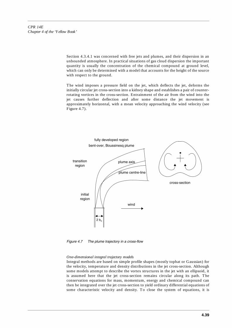
CPR 14EChapter 4 of the ‘Yellow Book’
4.39
Section 4.3.4.1 was concerned with free jets and plumes, and their dispersion in anunbounded atmosphere. In practical situations of gas cloud dispersion the importantquantity is usually the concentration of the chemical compound at ground level,which can only be determined with a model that accounts for the height of the sourcewith respect to the ground.
The wind imposes a pressure field on the jet, which deflects the jet, deforms theinitially circular jet cross-section into a kidney shape and establishes a pair of counter-rotating vortices in the cross-section. Entrainment of the air from the wind into thejet causes further deflection and after some distance the jet movement isapproximately horizontal, with a mean velocity approaching the wind velocity (seeFigure 4.7).
Figure 4.7 The plume trajectory in a cross-flow
One-dimensional integral trajectory modelsIntegral methods are based on simple profile shapes (mostly tophat or Gaussian) forthe velocity, temperature and density distributions in the jet cross-section. Althoughsome models attempt to describe the vortex structures in the jet with an ellipsoid, itis assumed here that the jet cross-section remains circular along its path. Theconservation equations for mass, momentum, energy and chemical compound canthen be integrated over the jet cross-section to yield ordinary differential equations ofsome characteristic velocity and density. To close the system of equations, it is
fully developed region
bent-over, Boussinesq plume
transitionregion
initialregion
wind
plume axis
plume centre-line
2 bo
cross-section

4.40
necessary to make further assumptions about the entrainment of air into the jet. Theintegral equations are of the form:
In the equation s is the axial coordinate of the jet or plume, and y is the radialcoordinate, perpendicular to the axis. ρ is the density and u the flow velocity in thejet, b is the width parameter of the jet and ρa is the density of ambient air. The termwe(s) can be interpreted as the entrainment velocity (cf. equation 4.16) and containscontributions from 3 processes:– Jet entrainment occurs due to the shear stress with the atmosphere.– Air is entrained by the velocity component of ambient wind, perpendicular to the
jet axis.– Entrainment due to atmospheric turbulence can be neglected close to the stack,
but not at larger distances where it becomes the dominant process.The functions φ and φa, represent the conserved physical quantity in the jet and inambient air. It can be equal to 1 (unity), or the horizontal velocity ux, or theconcentration c or the heat content cp ⋅∆T, leading to the conservation equations of,respectively, the total mass, the horizontal momentum, the chemical compound massand the thermal energy. The function f(s) is non-zero only in the momentumequation, where it represents a drag term which takes into account changes inmomentum due to the pressure field. It is a point of controversy whether the inclusionof drag forces in the momentum equation is really necessary. The set of equations iscompleted with the conservation equation for vertical momentum, in which case φequals uz, and the right-hand side of equation 4.18 includes the influence of thegravitational force.
In the equation the stratification of the atmosphere is not specified. The simplestplume trajectory models introduce two additional assumptions:– The distributions of physical quantities within the plume are constant (tophat
shape) at any given distance from the source.– The atmosphere is not stratified.The simplifications allow for an integration of the conservation equations over thewhole plume cross-section. The integrated version of equation 4.18 is:
Since by definition ∆Ta = 0 in an unstratified atmosphere, the integrated conservationequation of thermal energy implies that the buoyancy flux factor F is a conservedquantity, see also Section 4.2.7.1 and formula (4.2). It is a measure of the densitydifference between the jet and ambient air, and defined as:
d
ds----- ρ u φ 2 π y dy
o
2
b
∫ 2 π b ρ a φ a w e s ( ) f s ( ) += (4.18). φ kg m 1– s
1– ( )
d
ds----- ρu φ b 2 [ ] 2 π b ρ a φ a w e s ( ) f s ( ) += (4.19) φ kg m
1– s
1– ( )
F g ' u b 2 .= (4.20)(m 4 s -3 )
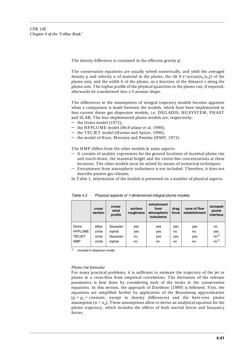
CPR 14EChapter 4 of the ‘Yellow Book’
4.41
The density difference is contained in the effective gravity g'.
The conservation equations are usually solved numerically, and yield the averageddensity
ρ
and velocity u of material in the plume, the tilt
θ
(=arctan(u
z
/u
x
)) of theplume axis, and the width b of the plume, as a function of the distance s along theplume axis. The tophat profile of the physical quantities in the plume can, if required,afterwards be transformed into a Gaussian shape.
The differences in the assumptions of integral trajectory models become apparentwhen a comparison is made between the models, which have been implemented infour current dense gas dispersion models, i.e. DEGADIS, HGSYSTEM, PHASTand SLAB. The four implemented plume models are, respectively:
–
the Ooms model (1972),
–
the HFPLUME model (McFarlane et al. 1990),
–
the TECJET model (Havens and Spicer, 1990),
–
the model of Hoot, Meroney and Peterka (HMP, 1973).
The HMP differs from the other models in some aspects:
–
It consists of analytic expressions for the ground locations of maximal plume riseand touch-down, the maximal height and the centre-line concentrations at theselocations. The other models must be solved by means of numerical techniques;
–
Entrainment from atmospheric turbulence is not included. Therefore, it does notdescribe passive gas releases.
In Table 1, information of the models is presented on a number of physical aspects.
Table 4.2 Physical aspects of 1-dimensional integral plume models
Plume rise formulae
For many practical problems, it is sufficient to estimate the trajectory of the jet orplume in a cross-flow from empirical correlations. The derivation of the relevantparameters is best done by considering each of the terms in the conservationequations. In this section, the approach of Davidson [1989] is followed. First, theequations are simplified further by application of the Boussinesq approximation(
ρ
=
ρ
a
= constant, except in density differences) and the bent-over plume
assumption (u = u a ). These assumptions allow to derive an analytical equation for theplume trajectory, which includes the effects of both inertial forces and buoyancyforces.
crosssection
cross-wind
profile
surfaceroughness
entrainmentfrom
atmosphericturbulence
dragforce
zone of flowestablishment
slumpedplume
interface
Ooms ellips Gaussian yes yes yes yes no
HFPLUME circle tophat yes yes no no yes
TECJET circle Gaussian no yes yes yes no
1)
1)
Included in dispersion model.
HMP circle tophat no no no no no
1)
4.42
Since the Boussinesq approximation and the bent-over plume approximation areused in the derivation of the trajectory equation, it is not intended for the calculationof properties close to the source. The plume rise due to initial momentum M
o
andinitial buoyancy F
o
contribute with a down-wind dependency of x
1/3
and x
2/3
,respectively. This implies that at distances further away from the source, the buoyantplume rise is the dominating term.
The formalism of Davidson is incomplete in the sense that it does not treat the effectsof atmospheric stratification and stability. As a consequence, the equations predict aninfinite plume rise, whereas in reality it is observed that the plume levels off at acertain height, after which it is influenced almost solely by the atmosphericconditions.
Assuming that the transition to a horizontal plume occurs at a down-wind distance x
r
and that the plume rise due to the initial momentum is relatively small, the finalplume rise is equal to
∆
h
r
= constant F
o1/3
/ u
a
(m) (4.21).
In equation 4.21, F
o
is the buoyancy flux factor of the source (defined by 4.20 withu
o
, g
o
' and b
o
). The constant has dimension (m
2/3
). It has been shown by Briggs[1969] that experimental observations of plume rise from tall stacks can be describedby equation 4.21, provided that the constant is a function of F and also of theatmospheric stability. Briggs has also derived expressions for momentum-dominatedplume rise, of the form
Here the constant has dimension (m
2/3
s
-2/3
).Many models of final plume rise have been proposed by Briggs and by other authors,and most of them assume the functional behaviour which is given in the aboveequations. They differ mainly in the way that the effects of atmospheric stability aretreated. A well-established model is presented in section 4.5.4.3
4.3.5 The modelling of dense gas dispersion
Our interest is in catastrophic releases of a chemical compound, with a largevolume or volume flow rate. Many hazardous volatile materials are heavier than air,for one or more of the following reasons:
–
The molecular weight of the chemical compound is higher than that of air.Examples are: LPG, cyclohexane, freon and chlorine.
–
The chemical compound is released as a cold gas, or cooled due to the evaporationprocess. Examples are: LNG, ammonia and hydrogen fluoride.
–
In case of a flashing release, the cloud is a mixture of aerosols and vapour. This isoften seen in ammonia releases.
–
Chemical reactions occur which are endothermic or result in the pick-up ofatmospheric water vapour. Reactive chemical compounds are ammonia, hydrogenfluoride and nitrogen tetroxide.
∆hr cons t / u a 2/3 tan = (4.22).(m)
CPR 14EChapter 4 of the ‘Yellow Book’
4.43
The temporal behaviour of the dispersion process is determined by the failure mode:
–
In an instantaneous release, a volume of gas is released in a very short time.Examples of instantaneous sources are severely ruptured vessels or rapidlyemptying pressurised tanks.
–
In a time-varying release the volume flow continues over a long period in anirregular way. An example is a liquid pool which is both spreading andvapourising.
–
A continuous release is characterised by a constant volume flow rate with asufficiently long duration for a steady state to be formed. Examples of this sourcetype are steady-state liquid pools and small ruptures in pipes and vessels.
The instantaneous release type differs from the other two in that along-winddispersion plays an important role in the dilution of the cloud.During the dispersion process of a dense (negatively buoyant) gas cloud, 4consecutive phases are observed:
–
The initial phase. The fluid motion is a strong function of the release conditions.
–
The gravity spreading phase. The entrainment is mainly due to the turbulencegeneration by the gravity-induced motion of the cloud.
–
An intermediate phase. Entrainment is due to an interplay between theatmospheric turbulence and gravitational forces.
–
The passive (neutrally buoyant) dispersion phase.The gravity spreading phase (see also Section 4.2.6) provides a good illustration ofthe effects which are typical for dense gas:
–
The density gradient induces gravity spreading in the horizontal direction. Thesegravity currents drive the flow within the cloud, independent of the atmosphericwind.
–
Mixing is primarily through the self-generated vortices at the edge of the cloud(also called gravity-front).
– Mixing by atmospheric turbulence at the top of the cloud is suppressed by thedensity gradient.
–
Turbulence within the cloud is reduced due to the stable stratification (i.e. anegative vertical density gradient) of the dense gas layer.
As a consequence, a dense gas cloud remains in the lower part of the atmosphere, witha large spread in the lateral direction. Meandering due to atmospheric turbulence isless than for passive clouds. Attempting to describe dense gases by adapting Gaussianmodels suitable for passive clouds is inherently inadequate, because the Gaussianmodels do not account for the momentum and energy effects.Present dense gas dispersion models can be roughly divided into 3 classes:
–
Phenomenological models, in which the dispersion behaviour is described by aseries of nomograms.
–
Intermediate models, such as box models and grounded plume models.
–
Advanced models which solve the Navier-Stokes equations.Except for models solving the three dimensional Navier-Stokes equations none of themodels describe the internal flow in the cloud, such as the vortex in the gravity front.A general description of the models in the 3 classes is given in the Sections 4.3.5.1-4.3.5.3.
4.44
4.3.5.1 Empirical relations of dense gas dispersion
Empirical relations between the observed physical quantities in dense gasdispersion experiments originate from laboratory simulations on a small-scale, orfrom field tests, or from both. Simple formulae based on dimensional arguments canexplain many observations of dense gas dispersion. It is, in general, not necessary tospecifically model the detailed flows inside the gas cloud, since the gross entrainmentintegrated over the cloud is important. The starting-point is an inventory of theindependent variables that are relevant in dense gas dispersion. They are:
–
The mean wind velocity u
a
.
–
The initial volume V
o
of the chemical compound (in case of an instantaneousrelease), or the volume flow rate v
o
(for time-varying releases).
–
The dimension b
o
of the source.
–
The density
ρ
o
of the chemical compound and ambient density
ρ
a
.Other variables, such as the atmospheric stability, the local roughness length and thesource geometry, are less important. A dimensional analysis yields the parametersthat determine the dispersion process:
x/b
o
, y/b
o
, z/b
o
, u
a
t/b
o
, u
a2
/(gb
o
),
ρ
o
/
ρ
a
, and either v
o
/(u
a
b
o2
) or V
o1/3
/b
o
.
Here x is the down-wind distance, y is the lateral coordinate, z is the height, t is thetime and g is the gravity constant. The number of parameters can be reduced furtherby: (1) considering only ground level concentrations, (2) assuming that at any down-wind distance the maximum concentration occurs on the centre-line, and (3)employing the Boussinesq approximation. In the Boussinesq approximation theparameters u
a2
/(gb
o
) and
ρ
o
/
ρ
a
can be replaced by a single parameter u
a2
/(g
o
'b
o
),
where g o ' = g( ρ o - ρ a )/ ρ a is the effective gravity at the source.
In an instantaneous release, the important dependent (output) variable is theconcentration of the chemical compound at the time of arrival of the cloud. Theconcentration attains its maximum value c
max
at that moment, and subsequentlydecreases with time as the cloud is advected past the point.
c
max
is made non-dimensional with the initial concentration c
o
expressed as thevolume of chemical compound per unit volume. For a source with an approximatelyspherical or cubic shape, the dimension b
o
of the source is proportional to V
o1/3
, andc
max
/c
o
depends on only 2 parameters: x/V
o1/3
and u
a2
/(g'
o
V
o1/3
).
In a time-varying or continuous release, the important dependent variable is the time-averaged concentration c
mean
.
The source dimension b
o
is less important further away from the source, as the plumeforgets its past history. Then c
mean
/c
o
again depends on 2 parameters: and.
The functional behaviour of the concentration values can be derived fromexperimental data and the resulting correlations can then be reproduced innomograms. This approach has been followed by Britter and McQuaid in theirWorkbook (1988), and also in the VDI Guideline 3783 part 2 (1990).
x ua/vo( )ua
5/2/ g'o vo( )
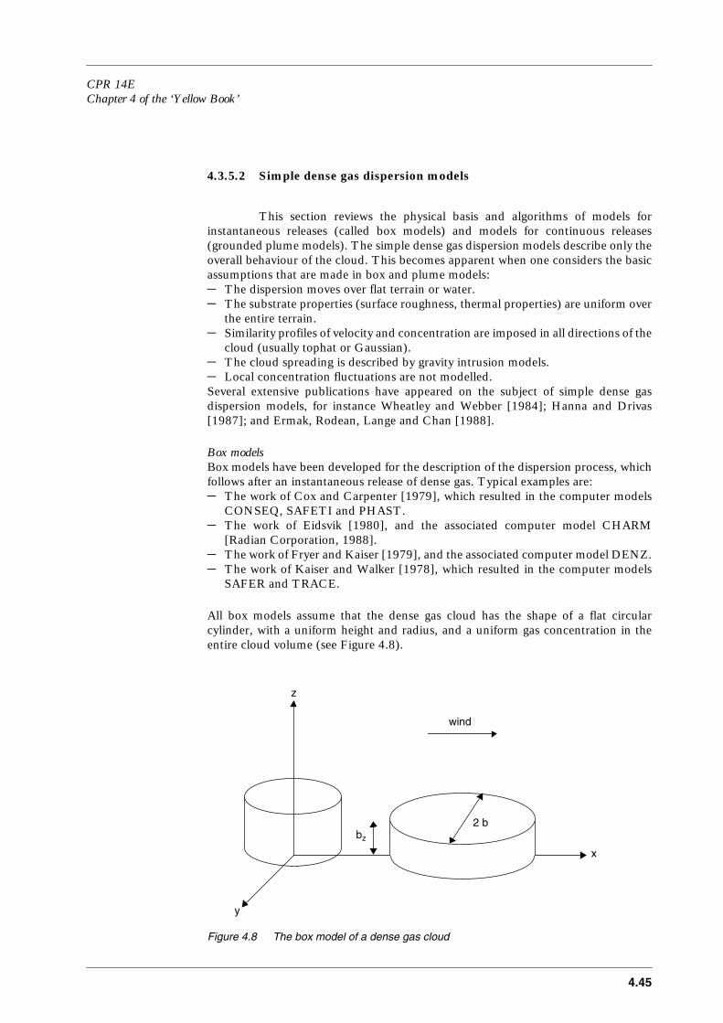
CPR 14EChapter 4 of the ‘Yellow Book’
4.45
4.3.5.2 Simple dense gas dispersion models
This section reviews the physical basis and algorithms of models forinstantaneous releases (called box models) and models for continuous releases(grounded plume models). The simple dense gas dispersion models describe only theoverall behaviour of the cloud. This becomes apparent when one considers the basicassumptions that are made in box and plume models:– The dispersion moves over flat terrain or water.– The substrate properties (surface roughness, thermal properties) are uniform over
the entire terrain.– Similarity profiles of velocity and concentration are imposed in all directions of the
cloud (usually tophat or Gaussian).– The cloud spreading is described by gravity intrusion models.– Local concentration fluctuations are not modelled.Several extensive publications have appeared on the subject of simple dense gasdispersion models, for instance Wheatley and Webber [1984]; Hanna and Drivas[1987]; and Ermak, Rodean, Lange and Chan [1988].
Box modelsBox models have been developed for the description of the dispersion process, whichfollows after an instantaneous release of dense gas. Typical examples are:– The work of Cox and Carpenter [1979], which resulted in the computer models
CONSEQ, SAFETI and PHAST.– The work of Eidsvik [1980], and the associated computer model CHARM
[Radian Corporation, 1988].– The work of Fryer and Kaiser [1979], and the associated computer model DENZ.– The work of Kaiser and Walker [1978], which resulted in the computer models
SAFER and TRACE.
All box models assume that the dense gas cloud has the shape of a flat circularcylinder, with a uniform height and radius, and a uniform gas concentration in theentire cloud volume (see Figure 4.8).
Figure 4.8 The box model of a dense gas cloud
2 b
wind
bz
x
z
y
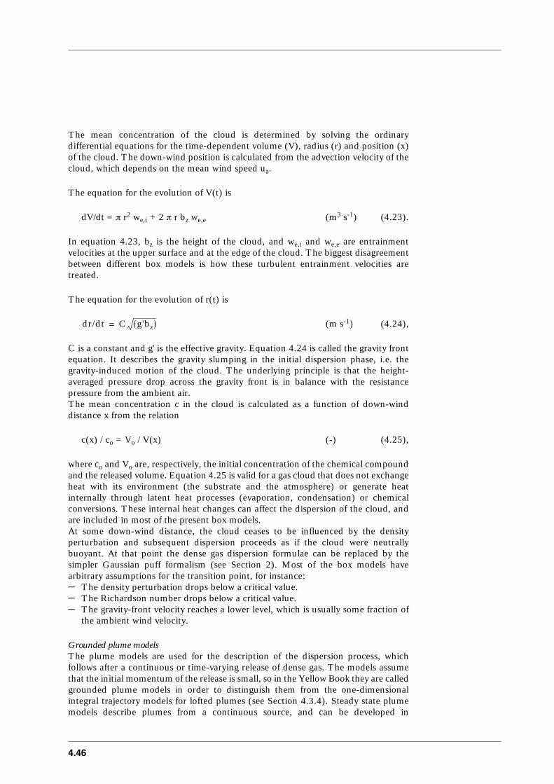
4.46
The mean concentration of the cloud is determined by solving the ordinarydifferential equations for the time-dependent volume (V), radius (r) and position (x)of the cloud. The down-wind position is calculated from the advection velocity of thecloud, which depends on the mean wind speed ua.
The equation for the evolution of V(t) is
dV/dt = π r2 we,t + 2 π r bz we,e (m3 s-1) (4.23).
In equation 4.23, bz is the height of the cloud, and we,t and we,e are entrainmentvelocities at the upper surface and at the edge of the cloud. The biggest disagreementbetween different box models is how these turbulent entrainment velocities aretreated.
The equation for the evolution of r(t) is
(m s-1) (4.24),
C is a constant and g' is the effective gravity. Equation 4.24 is called the gravity frontequation. It describes the gravity slumping in the initial dispersion phase, i.e. thegravity-induced motion of the cloud. The underlying principle is that the height-averaged pressure drop across the gravity front is in balance with the resistancepressure from the ambient air.The mean concentration c in the cloud is calculated as a function of down-winddistance x from the relation
c(x) / co = Vo / V(x) (-) (4.25),
where co and Vo are, respectively, the initial concentration of the chemical compoundand the released volume. Equation 4.25 is valid for a gas cloud that does not exchangeheat with its environment (the substrate and the atmosphere) or generate heatinternally through latent heat processes (evaporation, condensation) or chemicalconversions. These internal heat changes can affect the dispersion of the cloud, andare included in most of the present box models.At some down-wind distance, the cloud ceases to be influenced by the densityperturbation and subsequent dispersion proceeds as if the cloud were neutrallybuoyant. At that point the dense gas dispersion formulae can be replaced by thesimpler Gaussian puff formalism (see Section 2). Most of the box models havearbitrary assumptions for the transition point, for instance:– The density perturbation drops below a critical value.– The Richardson number drops below a critical value.– The gravity-front velocity reaches a lower level, which is usually some fraction of
the ambient wind velocity.
Grounded plume modelsThe plume models are used for the description of the dispersion process, whichfollows after a continuous or time-varying release of dense gas. The models assumethat the initial momentum of the release is small, so in the Yellow Book they are calledgrounded plume models in order to distinguish them from the one-dimensionalintegral trajectory models for lofted plumes (see Section 4.3.4). Steady state plumemodels describe plumes from a continuous source, and can be developed in
dr/dt C g 'bz( )=
CPR 14EChapter 4 of the ‘Yellow Book’
4.47
one-to-one correspondence with the already discussed box models, by replacing thetime variable t with the down-wind distance x from the source. A typical example isthe work of Jagger [1983]. This model employs the entrainment coefficients of Fryerand Kaiser [1979]. A computer model, CRUNCH, was also developed. The morerecent computer models (e.g. PHAST [Hanna et al., 1991], DRIFT [Webber et al.,1992], etc.) contain the box module and the plume module within a single package.In grounded plume models, it is assumed that a plume has a rectangular cross-sectionof height bz(x) and half-width b(x) (see Figure 4.9).
Figure 4.9 The grounded plume model of a continuous dense gas plume
The concentration c of the chemical compound and the advection velocity u areuniform over the entire area A(x) of the cross-section, and in general an empiricalrelation is assumed between this averaged value of u and the plume height bz.
The equation for the increase of total mass is
d(ρ u A)/dx = 2 ρa b we,t + 2 ρa bz we,e (kg m-1 s-1) (4.26).
ρ and ρa are, respectively, the densities of the plume gas and of ambient air. we,t andwe,e are entrainment velocities at the upper surface and at the edge of the plume.Because of the similarity between the equations 4.23 and 4.26, a plume modelequivalent can be built for each box model, by assuming the same closure relationsfor the entrainment. The equation for the evolution of b(x) is
C is a constant, and g' is the effective gravity. It should be noted that gravitationalslumping, and also mixing, in the longitudinal direction is neglected in the steady-state plume model. This is justifiable in sufficiently high-wind conditions.The concentration decay as a function of down-wind distance is obtained by solvingthe equation of compound species flux simultaneously with the equations 4.26 and
2 b
wind
bz
x
z
u db/dx C g ' b z ( ) = (4.27),(m s -1 )

4.48
4.27. It is noted that, for simplicity, the internal heat changes have been neglected inthe equations, whereas they are incorporated in most of the present steady stateplume models.If the plume material is removed from the source at a lesser rate than the flow ratefrom the source, then plume material is accumulated at the source. The accumulationis accompanied by horizontal, buoyancy-induced motions providing a much largerplume area near the source. As a result the effective source size can be much largerthan the physical source size. Most of the present plume models contain an algorithmto describe the formation of the secondary source blanket.A different technique to simulate a steady release is to divide the total release into anumber of puffs, each of which is considered as a separate release. This technique isused in the CHARM computer model.
Generalised plume models
Generalised steady state plume models give greater structure to the spatial variationsof the dense gas concentration than merely assuming a rectangular or Gaussianprofile. This enables a greater range of physical processes to be modelled, and certainprocesses to be more realistically modelled. A well-known example is the model ofColenbrander [1980], where similarity forms for the concentration profiles presentthe plume as a horizontally homogeneous centre section with Gaussian concentrationprofile edges (see Figure 4.10).
Figure 4.10 The down-wind development of the concentration profiles in vertical and lateral direction, in a generalised plume model. The dashed curve is the LFL isoconcentration contour
wind
c
z
1
clfl clfl clfl
1 1
c
y
1
clfl clfl clfl
1 1
x
x
CPR 14EChapter 4 of the ‘Yellow Book’
4.49
In formula:
c(x,y,z) = c
c
(x) F
y
(y) F
z
(z), (kg m
-3
or parts per unit volume)
F
y
(y) = 1 for
y
≤
b,
F
y
(y) = exp(-(
y
-b(x))
2
/
σ
y
(x)
2
) for
y
> b,
F
z
(z) = exp(-(z /
σ
z
(x))
2
) (4.28).
The model is formulated in terms of eddy-diffusivities rather than entrainmentvelocities. This means that the diffusion equation is solved in the vertical and lateraldirection.
This way of formulating the plume model guarantees that the transition to passivebehaviour in the edge entrainment and lateral spreading is continuous. The model ofColenbrander has been implemented in computer models such as HEGADAS[McFarlane et al., 1990] and DEGADIS [Havens, 1989].
Time-varying releases
In some cases (e.g. a spreading and vaporising liquid pool) the volume flow rate of therelease will show variations with time, and this will also affect the concentration levelsin the resulting plume. Colenbrander [1980] has proposed to describe a time-varyingrelease with the concept of travelling observers. The concept consists of 4 steps:
–
Observers travel at a series of times with the wind, starting upwind of the pool.
–
The pool data observed by each observer are determined.
–
For each observer, the concentration is computed via a steady state plume model,adopting the observed pool data. The concentration at time t for a certain down-wind distance is determined by calculating the positions of observers at times t.
–
At time t, the actual concentration is determined from a Gaussian integration withrespect to down-wind distance of all observer concentrations. The Gaussianintegration involves the longitudinal diffusion by means of a down-winddispersion coefficient
σ
x
.In formula:
(u
a
t) is the position at time t of an observer travelling with the wind in the down-winddirection. At this position the observer observes the concentration c
c
(u
a
t), which isobtained from a steady state plume model. An often used expression for thedispersion coefficient is
σ
x
(x) = 0.13 x (see also Sections 4.3.3 and 4.5.3.3 on theGausian plume model).
cc x,t( ) c∫ c uat( )/ 2π( )σx uat( )( ) exp 0.5 x uat – ( ) – 2
/ σ x uat ( ) 2 ( ) duat = (4.29).

4.50
4.3.5.3 The conservation equations for a dense gas release
The full equations describing the release of a dense gas are the Navier-Stokes equations for the instantaneous velocity and density fields. The Navier-Stokesequations are partial differential equations expressing the conservation of total massand the conservation of compound species (the continuity equations), theconservation of enthalpy, and a 3-vector equation of motion. An equation of state isalso required. The equations are averaged to obtain equations for the mean fields. Inthe application of the Navier-Stokes equations to gas dispersion processes, aconvenient set of independent fields is formed by the velocity, the temperature, thedensity and the concentration of the chemical compound. The pressure field is notincluded, since the mixture of air and dense gas is assumed to be incompressible. Aturbulence closure scheme is needed for the description of correlations of fluctuatingquantities.There are dispersion models which attempt to solve, by means of numericaltechniques, the Navier-Stokes equations in 3 dimensions, but their development isnot at a sufficiently advanced stage that the models can be used routinely. At themoment, the 3-dimensional models can best be viewed as a research tool in the studyof the flow field of dispersed clouds. The costs of undertaking a fully 3-dimensionalsimulation also tend to be significantly greater than the costs of using simpledispersion models. For these reasons the 3-dimensional models are excluded from adiscussion in the Yellow Book. An overview of 3-dimensional dense gas dispersionmodels can be found in the study of Ermak et al. [1988].
The shallow layer theory is related to the 3-dimensional approach. It is based on thefull set of conservation equations, but advantage is taken of the simple structure ofdense gas clouds in cross-wind planes. The computational effort is greatly reduced byregarding the cross-wind variables as depending only on time and down-winddistance.
Zeman [1982] has developed the formalism to describe the dispersion of a dense gasrelease in the presence of wind by means of a 1-dimensional shallow layer model. Arecent computer implementation based on the formalism is the SLAB model [Ermak,1990]. The discussion in this section starts with the shallow layer formulation for acontinuous grounded plume, and subsequently treats the case of an instantaneouscloud.
The shallow layer plume model
The fields of physical quantities in a plume are regarded as depending only on down-wind distance x, and are averaged in the cross-wind direction. The conservationequations in the shallow layer plume model are equivalent to the equations for a 1-dimensional integral plume model, with additional terms in the former set ofequations for the description of the gravitational slumping on the ground. The maindifference between the two sets is that the averaging of the fields in the integral plumemodels is done over the plume cross-sections, and in the shallow layer theory it isdone over the cross-wind cross-sections. This implies that the shallow layer equationscan be used for lofted plumes in the region where the plume has been bent-over bythe wind.The shallow layer plume model and the steady state grounded plume model, whichwas discussed in the previous section, differ in their treatment of momentumconservation. In the shallow layer approach, the vector equation of momentum

CPR 14EChapter 4 of the ‘Yellow Book’
4.51
conservation is solved, whereas the steady state grounded plume model solves thegravity slumping equation (4.27).
The shallow layer cloud model
In the shallow layer model of Zeman [1982], the puff is treated as a grounded cloudwith a half-length b
x
, a half-width b
y
and a height b
z
. The independent variable is thedown-wind travel time t of the cloud centre-of-mass. The fields of physical quantitiesin the cloud are averaged over the cloud volume V = 4b
x
b
y
b
z
.Air is entrained in the down-wind and cross-wind sides of the cloud, with differententrainment rates, and at the upper surface of the cloud. The difference between theshallow layer formalism and the box formalism is in the description of gravityslumping. The shallow layer approach solves a vector equation of motion forthe gravity spreading, whereas the box models are based on the gravity frontequation (4.24).The shallow layer cloud model can also be applied to releases above ground level. Theterms in the conservation equations for gravity spreading must then be replaced byterms which describe a sinking cloud.
4.52
4.4 Selection of models
4.4.1 Introduction to Section 4.4
In Section 4.4 the considerations which have led to the selection of modelswhich are included in Section 4.5, are explained. In general the selection is based onconsiderations with respect to:
–
The degree to which a model is able to describe the physical phenomena correctly(validation and verification).
–
The general acceptance of a model.
–
The degree to which a model is flexible to input and output requirements(applicability and ease of use).
–
The transparency and internal consistency of a model (i.e. the consequent use ofclear principles and assumptions).
These considerations are presented as follows:
–
Section 4.4.2 addresses methods to calculate atmospheric stability and quantitiesin the mixed layer such as wind speed and turbulence.
–
Section 4.4.3 addresses selection of dispersion parameters in Gaussian plumemodels for passive dispersion.
–
Section 4.4.4 addresses mainly the selection of integral models for jets and plumesin ambient wind.
– Section 4.4.5 addresses the selection of dense gas dispersion models.
4.4.2 Schemes for atmospheric stability categories and meteorological data
4.4.2.1 Atmospheric stability catagories
Most widely-used dispersion models make use of the Pasquill-Giffordstability categories (A-unstable to F-stable) and parametrisations of the local lateraland vertical plume width (σy and σz).However, already Pasquill and Smith [1983] point out the restrictions of thesequalitative schemes in favour of schemes using quantifications of physical parametersof the boundary layer. At the European Workshop ‘Objectives for Next Generationof Practical Short-Range Atmospheric Dispersion Models’ [Olesen, 1992] it wasgenerally agreed that up-to-date models should use these types of stability schemes.Such a scheme is the scheme developed by Holtslag et. al. (see Section 4.3.2).This scheme can be coupled directly with calculation of dispersion parameters as afunction of Monin-Obukhov length, plume height and down-wind distance or traveltime. This approach leads to good agreement with observations [Gryning et. al.,1987].There is a number of additional advantages of the ‘Holtslag’-scheme and the relatedmethodology for calculation of dispersion parameters:– The scheme is applicable to all climatological zones;– The calculation of dispersion parameters can be extended to very low wind speed
conditions.
CPR 14EChapter 4 of the ‘Yellow Book’
4.53
However, we have to acknowledge the fact that long-term meteorological data is veryoften available in terms of Pasquill stability classes. Therefore use will be made ofGolder’s scheme [1972], see Figure 4.11, to relate Pasquill classes to roughnesslength and Monin-Obukhov length and vice versa.
For stability over sea the scheme by Hsu [1992], see Figure 4.12, will be adopted.
4.4.2.2 Variation of wind speed
All dispersion models (passive dispersion models and dense gas dispersionmodels) need information about the vertical variation of wind speed. For wind speedsin the surface layer the use of the Businger-Dyer relations is selected [Panofsky andDutton, 1984]. These relation use roughness length and Monin-Obukhov length asinput.
4.4.2.3 Variation of turbulence
Some application of dispersion parameters for Gaussian plume modelsrequire the standard deviation of turbulent velocities in cross-wind and verticaldirection. From available suggestions to calculate the variation of these turbulentquantities the expressions by Gryning et. al. [1987] are selected with a change of theproportionality constant in order to make them consistent with the surface-layer dataof turbulence provided by Panofsky and Dutton [1984].
4.4.2.4 Determination of mixing height
No selection of mixing height can be made which is valid for all locations.For applications in the Netherlands the expressions for stable conditions aspresented in Section 4.3.2.2 are selected. For near neutral conditions (Pasquillclass D) a combination is selected from the expression in Section 4.3.2.2 and a fixedvalue of 500 m. For Pasquill class C a value of 1000 m and for Pasquill A and Ba value of 1500 m is used.
4.4.3 Selection of models for passive dispersion
4.4.3.1 Selection of model type
For passive dispersion the use of the Gaussian plume model is selected forall scaling regions in the mixing layer (Figure 4.5). For the surface layer and themixing layer other models provide better agreement with reality, but they are muchless flexible with respect to source height, source dimensions and output.
4.54
4.4.3.2 Dispersion parameters
Gaussian plume models make use of two (for continuous releases) or three(for instantaneous releases) dispersion parameters σx, σy, σz.
The dispersion parameters σx, σy, σz of the 2nd edition of CPR14E are used (see section4.5.3.4).
4.4.4 Selection of models for jets and plumes
This section indicates which jet and plume models have been selected fromthe survey in Section 4.3.4.
Jets and plumes in still airThe theory of jets and plumes is based on similarity principles. The fixation of theempirical constants in the expressions by Chen and Rodi [1980] and their usage ofGaussian profiles for the physical distribution functions in a cross-section havebecome widely-accepted, and is therefore selected for a more detailed discussion.
One-dimensional integral trajectory modelsAt present it is not possible to make a conclusive statement which of the various1-dimensional integral plume models is preferable. However, in many cases themodel will be used as a front-end module to a dense gas dispersion model, and thecoupling of the models will impose additional model requirements. If the loftedplume model has to be coupled to a grounded steady plume model, which can onlytreat surface area sources, then the plume touch-down and slumping have to bemodelled separately. On the other hand, if the lofted plume model acts as a front-endmodule to a model that is based on solving the conservation equations, then it issufficient for the lofted plume model to describe the initial phase of plume rise anddown-wind bending of the plume. The dense gas dispersion model, which isdiscussed in Section 4.5.5, is of the last-mentioned type. The model of Hoot et al.[1973] is easy to couple to this dense gas dispersion model, and it is one of thesimplest integral trajectory models, and for these reasons is treated in greater detail.
Plume rise formulaeThe selected plume rise formulae are based on an early publication of Briggs [1969],which has become widely-accepted. During the development of the ‘Dutch NationalModel’ [Dutch committee on the dispersion of air pollution, 1984] some additionswere made in order to extend the validity to tall stacks and to all atmospheric stabilityconditions. These additions deal 1) with the criterium for final plume rise in neutralatmosphere, and 2) with plume rise in stable atmosphere. The adaptions areincorporated in the set of selected formulae.
CPR 14EChapter 4 of the ‘Yellow Book’
4.55
4.4.5 Selection of dense gas dispersion models
Criteria for model selectionThe criteria for selection of a dense gas dispersion model relate to three aspects, i.e.operational requirements (ease of use), physical plausibility, and educational aspects(transparency of the model).
The operational requirements are:I The model is usable in operational conditions. Constraints on cost and time are
imposed by the operational environment, and the sophistication and efficiency ofthe algorithms in the physical model should be compatible with these constraints.It is emphasised that it is not the intention to evaluate the user-friendliness of thesoftware implementations of models. There is a continuous improvement in thisarea, and available computer models can be adapted to the needs of the userwithout great effort.
II The model is current. In other words, the model is supported by an organisation,and the model is widely used. Currency of usage can for instance be assessed fromthe frequency of references in the recent (1983-1993) scientific literature.
III The model allows for coupling of source term models and explosion/fire models.
It is desirable that the model is based on plausible physical assumptions. For densegas modelling, Wheatley and Webber [1984] have formulated this in terms of 3objectives:I In the model, the transition between the dense gas phase and passive phase of
dispersion should be continuous.II The model should include all turbulent dilution mechanisms (jet entrainment,
shear production and enhanced entrainment from gravity spreading, convection).III The modelling of entrainment should be consistent with results of laboratory
experiments on entrainment in stratified flows.Concerning output requirements, within its range of validity the model should give afair description of the actual gas dispersion in a realistic release situation. This isformulated by Wheatley and Webber as a 4th objective:IV The model should realistically describe the ensemble-average spatial
concentration distribution in both the dense gas phase and in the passive phase ofdispersion.
From an educational point of view, it is preferred to have a few models with wideapplicability instead of many models with restricted applicability.
The selection procedureDense gas dispersion models for operational use can be divided into 2 classes:I Phenomenological models, in which the dispersion behaviour is described by a
series of nomograms (see Section 4.3.5.1);II Intermediate models, such as box models and models based on shallow layer
theory (see Sections 4.3.5.2 and 4.3.5.3).Many of the models are available as computer codes; they often contain source andjet models to describe the initial phase of the dense gas release. The selection ofsource models is not part of the present chapter; this topic is discussed in theChapters 2 and 3 of the Yellow Book. The selection of jet models is discussed inSection 4.4.4.

4.56
A useful reference document for the assessment of models is the report of Hanna etal. [1991] on an extensive model evaluation project of 14 dispersion models. Theproject was initiated because there were no standard objective quantitative means ofevaluating the dense gas dispersion models.In the project of Hanna et al. a system has been developed to evaluate theperformance of microcomputer-based dispersion models that are applicable tochemical releases into the atmosphere. The study is better than previous dense gasdispersion model evaluation projects because a method was developed which givesconclusive results. Following this work, Hanna and Chang [1992] have reviewed theHGSYSTEM package in the same way as the other 14 models.
The Workbook of Britter and McQuaid [1988] is widely-accepted as a reference textfor dense gas dispersion. The nomograms in the book were evaluated by Hanna andturned out to give a good description of experimental data sets.Therefore, the Workbook is selected in the Yellow Book as a representative of class Imodels. A detailed discussion of the Britter and McQuaid model is presented inSection 4.5.5.1.
In the reports of Hanna et al. it is concluded that HEGADAS (and also theHGSYSTEM package, which contains HEGADAS as a module) has a goodperformance for continuous dense gas and passive releases, but it is not intended formodelling instantaneous releases.The models CHARM, PHAST and SLAB have an acceptable performance for all ofthe gas releases included in the study of Hanna (i.e. continuous and instantaneousdense gas releases, and continuous passive gas releases). CHARM and PHAST areproprietary models, HEGADAS and SLAB are publicly available.Since the performances of HEGADAS, CHARM, PHAST and SLAB are allacceptable, the selection of a model for a more detailed discussion was based oneducational aspects. The SLAB computer model makes use of shallow layer theory(see Section 4.3.5.3), which has the advantage that the physical processes of densegas dispersion are formulated in a transparent way. The SLAB model is describedextensively in Section 4.5.5.2, as a representative of class II models.It should be mentioned that, compared with the other 3 acceptable models, SLABmight underpredict concentrations near to the source [Hanna et. al., 1991].
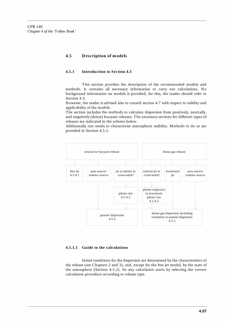
CPR 14EChapter 4 of the ‘Yellow Book’
4.57
4.5 Description of models
4.5.1 Introduction to Section 4.5
This section provides the description of the recommended models andmethods. It contains all necessary information to carry out calculations. Nobackground information on models is provided, for this, the reader should refer toSection 4.3.However, the reader is advised also to consult section 4.7 with respect to validity andapplicability of the models.The section includes the methods to calculate dispersion from positively, neutrally,and negatively (dense) buoyant releases. The necessary sections for different types ofreleases are indicated in the scheme below.Additionally one needs to characterise atmospheric stability. Methods to do so areprovided in Section 4.5.2.
4.5.1.1 Guide to the calculations
Initial conditions for the dispersion are determined by the characteristics ofthe release (see Chapters 2 and 3), and, except for the free jet model, by the state ofthe atmosphere (Section 4.5.2). So any calculation starts by selecting the correctcalculation procedure according to release type.
neutral or buoyant release dense gas release
free jet area source/volume source
jet or plume incross-wind?
plume rise
passive dispersiondense gas dispersion includingtransition to passive dispersion
vertical jet incross-wind?
horizontaljet
area source/volume source
plume trajectoryto maximumplume rise
4.5.4.1
4.5.4.2
4.5.5
4.5.4.2
4.5.3

4.58
Step 1
Has the release a high initial momentum?– Yes: Use the free jet model in Section 4.5.4.1. Check the validity of the model
1) by applying the conditions provided in formulae (4.71-4.72), and 2) byensuring cross-wind (for vertical jets) has not bent the plume over in theregion of interest (jet velocity should exceed ambient velocity by a factor of10). If the model is not valid, proceed with steps 2, 3, 4 or 5.If beyond the jet region atmospheric dispersion is of interest, proceed alsowith steps 2, 3, 4 or 5.
Step 2
– Determine the roughness length of the area of interest, using Table 4.3, Section4.5.2.1.
Step 3
– Determine stability of the atmosphere by calculating the Monin Obukhov lengthand the friction velocity according to Sections 4.5.2.2, 4.5.2.3 and 4.5.2.4. Itmight be necessary to use the expressions provided in Section 4.5.2.1.
Step 4
Determine whether the release will lead to a cloud denser than the ambient air.– No: Proceed with step 5.– Yes: Step 4.1
Is the release instantaneous?– Yes: Decide whether a fast solution or a complex solution is preferred.
For a fast solution, proceed by using the Britter and McQuaidnomogram Figure 4.15 and Diagram 4.1, Section 4.5.5.1.Otherwise, use the SLAB-model, Section 4.5.5.2, Diagram 4.10.
– Step 4.2Is the release continuous?– Yes: Step 4.2.1.
Is the release a vertical jet and this jet be ignored?– Yes: Use the HMP-model, Section 4.5.4.2, to determine
maximum plume rise and concentration.Thereafter, couple the results with the SLAB-model(formulae 4.107-4.112, Diagram 4.6, Section 4.5.5.2),and proceed the calculation with the continuous SLAB-model (Diagram 4.4).
– No: Decide whether a fast solution or a complex solution ispreferred. For a fast solution, proceed by using theBritter and McQuaid nomogram Figure 4.17 andDiagram 4.2, Section 4.5.5.1.Otherwise, use the SLAB-model, Section 4.5.5.2,Diagram 4.4.

CPR 14EChapter 4 of the ‘Yellow Book’
4.59
– Step 4.3Is the release of finite duration?– Yes: Decide whether a fast solution or a complex solution is preferred.
For a fast solution, use the Britter and McQuaid nomograms andfollow the instructions at the end of Section 4.5.4.1.Otherwise, use the SLAB-model, Section 4.5.4.2, and follow theinstructions related to Diagram 4.9.
Step 5
The release is non-buoyant or positively buoyant.– Step 5.1
Is the release instantaneous?– Yes: Apply the Gaussian model as introduced in formula 4.52 and use
Sections 4.5.3.1, 4.5.3.2, and 4.5.3.3. If necessary, apply formula 4.65numerically to calculate flammable mass.
– Step 5.2Is the release continuous?– Yes: Apply the Gaussian model as introduced by formula 4.51 and use
Sections 4.5.3.1, 4.5.3.2, and, if necessary, 4.5.3.4. Applyapproximations 4.66-4.70 to calculate flammable mass.
– Step 5.3The release is time-dependent.– Apply the Gaussian model as introduced in formulae 4.51 and 4.52. Use
Sections 4.5.3.1, 4.5.3.2, and 4.5.3.3, but note the Sections 4.5.3.5 and4.5.3.6. Use formula 4.65 numerically to calculate the flammable mass.
4.5.2 Models to determine atmospheric stability and vertical variation of wind speed
Atmospheric stability is determined by the Monin-Obukhov length Land/or the Pasquill stability class.This section provides techniques to calculate Monin-Obukhov length L from routinemeteorological data (Section 4.5.2.2), from Pasquill stability class (Section 4.5.2.3),and over sea (Section 4.5.2.4).First, however, in Section 4.5.2.1, methods to determine vertical variation of velocityand other relevant characteristics will be presented, as these are to be used during thecalculation of stability in Section 4.5.2.2 and for application in dispersion models.Additional properties of the atmosphere are presented in Sections 4.5.2.5 through4.5.2.6.
4.5.2.1 Calculation of vertical variation of velocity and temperature
The necessary data to calculate the vertical variation of wind speed are:– wind speed at specified height z (e.g. at 10 m height);– surface roughness length zo, using Table 4.3;– an estimate of the Monin-Obukhov length L, from Section 4.5.2.2.

4.60
The roughness length should be representative for the whole area over whichdispersion calculations are performed. Of course, different values for zo may be usedfor different wind directions. It should also be noted that the upwind area has aninfluence on the turbulence characteristics of the atmosphere. The atmosphere is inequilibrium with the (new) roughness length over a height of approximately one tenthof the down-wind distance from a change in roughness length.
The surface friction velocity u* can be calculated from velocity ua(z) at specifiedheight z as follows:
(if z > 100 m; use z = 100 m)
(the determination of L and u* is coupled. Section 4.5.2.2 provides methods tocalculate u* and L iteratively)and inversely the velocity at an arbitrarily height z from the friction velocity:
(if z > 100 m; ua(z) = ua(100 m))
κ is the Von Karman constant; κ = 0.4. The function f(z/zo,L) is defined as:
u* κ . u
a
z
( )
f z / z
o
,L
( )
-------------------- = (4.30)(m s -1 )
ua z( )u*
κ----- . f z / z o ,L ( ) = (4.31)(m s -1 )
f z/zo,L( ) ln z
zo---- 5
z zo–( )
L----------------+= for 1/L > 0
f z/zo,L( ) ln z
zo---- Ψ–
z
L---- Ψ
zo
L---- +=
(4.32)
for 1/L ≤ 0
(-)
Here Ψ z
L--- 2 ln
1
Ψ
'
+
2 ------------- ln
1
Ψ
'
2
+
2 ----------------
2 arctan Ψ ' ( ) – π
2
--- + +=
Ψ' 1 16z
L---–
1/4
=

CPR 14EChapter 4 of the ‘Yellow Book’
4.61
Table 4.3 Terrain classification in terms of aerodynamical roughness length z
o
,by Wieringa, [Holtslag, 1987])
For stable conditions, Section 4.5.2.2, it is necessary to calculate temperaturedifferences in the surface layer. These are calculated as follows (for 1/L > 0):
Γ
d
is the dry adiabatic lapse rate (0.011 K m
-1
).
Τ
*
is the turbulent temperature scale,to be calculated from the Monin-Obukhov length-scale L and surface frictionvelocity:
Here T
a
is temperature at about 2 m height (K).
Note that these formulae are valid for let say z > 10
⋅
z
o
, meaning that u
a
> u
*
inpractical situations.
4.5.2.2 Calculation of Monin-Obukhov length from routine meteorological data
The input for calculation of Monin-Obukhov length L requires:
–
cloud cover N;
–
wind speed at specified height z
u
(normally 10 m), u
a
(z
u
);
–
temperature at specified height z
T
(normally 2 m) T
a
;
–
roughness length z
o
;
–
solar elevation
χ
(from position, latitude and longitude, date and time, seeAppendix 1);
–
wet bulb temperature at z
T
(only for night-time condition) T
w
.
Class Short terrain description z
o
(m)
1 Open water, fetch
1)
at least 5 km
1)
The upwind length over water should be at least 5 km.
0.00022 Mud flats, snow; no vegetation, no obstacles 0.0053 Open flat terrain; grass, few isolated obstacles 0.034 Low crops; occasional large obstacles, x/h > 20
2)
2)
Here x is a typical upwind obstacle distance and h the height of the corresponding major obstacles.
0.105 High crops; scattered obstacles, 15 < x/h < 20
2)
0.256 Parkland, bushes; numerous obstacles, x/h < 15
2)
0.57 Regular large obstacle coverage (suburb, forest) (1.0)
3)
3)
These values are rough indications. The presented dispersion models do not account for obstacle effects. The reader should also consult section 4.7.5.
8 City center with high- and low-rise buildings (3)
3)
Ta z2( ) Ta z1( )–T*
κ------ln
z2
z1
---- 5
z2 z1–
L--------------+
Γd z2 z1–( )–= (4.33)(K)
T*
u*2 . T a
κ g L ---------------
=
(4.34)(K)

4.62
The Monin-Obukhov length can be calculated from the sensible heat flux H
o
whenthe surface friction velocity u
*
is known. (Normally, L and u
*
need to be calculatediteratively.)
(m) (4.35)
The next subsections will provide methods to estimate the sensible heat flux.Alternatively, L can be determined from a Pasquill stability class (Section 4.5.2.3), ortemperature difference with sea water (Section 4.5.2.4).
Estimate of sensible heat flux for day-time conditions
During day-time conditions, i.e. between local sunrise and sunset (where sunrise andsunset may be later or earlier, respectively, than the astronomical times due to shadingby mountains), the sensible heat flux H
o
is dependent on the net radiative heat fluxH
r
at the surface. Therefore first the incoming solar radiation H
rs
is to be calculateddepending on solar elevation
χ
and cloud cover N:
H
rs
= (C
1
. sin
χ
- C
2
) . (1 - 0.75 . N
3.4
) (J m
-2
s
-1
) (4.36)
Here C
1
= 990 J m
-2
s
-1
, and C
2
= 30 J m
-2
s
-1
.Including incoming and outgoing long wave radiation the net radiation H
r
iscalculated as
H
r
= (1 - e) . H
rs
+ C
3
T
a6
-
σ
. T
a4
+ C
4
. N/1.12 (J m
-2
s
-1
) (4.37)
Here
σ
is the Stefan-Boltzmann constant (5.67.10
-8
W m
-2
K
-4
), C
3
= 5.31.10
-13
J K
-6
m
-2
s
-1
, C
4
= 60 J m
-2
s
-1
, and e the albedo. Values of e are tabulated inTable 4.4.
Table 4.4 Albedo for various surfaces from Byrne et al. [1992]
Surface Albedo e
Soils (Dark, wet - Light, dry) 0.05 - 0.40Desert 0.20 - 0.45Grass (Long [1.0 m] - Short [0.02 m]) 0.16 - 0.26Agricultural crops 0.18 - 0.25Orchards 0.15 - 0.20Forests Decious (bare-leaved) 0.15 - 0.20 Coniferous 0.05 - 0.15Water 0.03 - 1.00Snow (Old - Fresh) 0.40 - 0.95Ice Sea 0.30 - 0.45 Glacier 0.20 - 0.40Tarmac, Asphalt 0.05Buildings 0.20 - 0.45
L ρacp T a u *
3
κ g H o -------------------------
–=
p

CPR 14EChapter 4 of the ‘Yellow Book’
4.63
The soil heat flux is estimated to be 10% of the net radiative heat flux; the remainingheat flux is divided between latent heat flux and sensible heat flux.
The sensible heat flux then reads:
Here C
5
= 20
J m
-2
s
-1
, and
γ
is the ratio of specific heat of air at constant pressure tolatent heat of evaporation of water, and to the rate of change of the saturation specifichumidity with temperature (values of
γ
are tabulated in Table 4.5).
Table 4.5 The dependency of the ratio
γ
on temperaturefor standard pressure (= 1000 mbar)
α
, the moisture availability constant, depends on the surface moisture condition (0
≤α ≤
1). If sufficient moisture is available for evaporation, like a grass-covered surfacein The Netherlands,
α
= 1; for dry bare soil
α
= 0.
When temperature T
a
and sensible heat flux H
o
are known, L and u
*
can be solvedby iteration. The iteration starts by calculating u
*
for 1/L = 0 (neutral condition).Normally 3 iterations are sufficient to achieve an accuracy of 5% in L.
Estimate of sensible heat flux for night-time conditions
Estimates of Monin-Obukhov length L and friction velocity u
*
for night-timeconditions are also based on the surface heat fluxes. In this case the four terms in theheat balance, viz. the net long wave radiation H
r
; the sensible heat flux H
o
; the latentheat flux H
l
; and the ground heat flux H
g
, which are all direct or indirect functions ofL and/or u
*
, are to be calculated. The total sum of heat fluxes needs to be zero, thus:
T
a
(˚C)
γ
-5 2.010 1.445 1.06
10 0.7915 0.6020 0.4525 0.3530 0.2735 0.21
H o 1
α
–
( ) γ
+
1
γ
+ ------------------------ 0.9 H r ( ) C 5 α –= (4.38)(J m -2 s -1 )
Ho Hl Hg Hr–+ + 0= (4.39)(J m-2 s-1)

4.64
This can only be obtained by an iterative procedure, e.g. the method of regula falsi,for which 1/L = 0 (neutral conditions) and 1/L = 1 (extremely stable) are appropriatestarting values.
For each step in the iterative procedure, u
*
and T
*
need to be calculated by means offormulae (4.30) and (4.34) from Section 4.5.2.1 above, using the current estimate ofL and using measured values of wind speed u
a , roughness length z
o , and temperature
at so-called screen height (about 2 m).The scheme requires introduction of temperatures at different levels:T
a
: temperature at ‘screen height’ (about 2 m).T
w
: wet bulb temperature at 2 m.T
r
: temperature at reference height of 50 m.T
o
: temperature at height of roughness length z
o
.T
s
: surface (vegetation) temperature.
T
r
and T
o
are calculated using the relation (4.33) from Section 4.5.2.1T
s
can be calculated over land from:
Here C
6
= 4.2 m s
-1
.Now the expressions for the four heat fluxes used in formula (4.39) will be given. Itis useful to define an intermediate step, the so-called isothermal net long waveradiation H
ri
:
where
σ
is the Stefan Boltzmann constant, C
7
= 9.35.10
-6
K
-2
, C
8
= 60 J m
-2
s
-1
, andN cloud cover.
The net long wave radiation H
r
is then:
The sensible heat flux H
o
follows from (4.34) and (4.35):
Here
ρ
a
is the density and c
p
the specific heat of air.
The ground heat flux H
g
follows from:
Ts To T*– 10C6
u*------+
= (4.40)(K)
Hri σ T r 4 1 C 7 T r
2 ⋅ – ( ) – C 8 N+= (4.41)(J m
-2 s -1 )
Hr Hri 4σ T r 3 T r T s – ( ) += (4.42)(J m -2 s -1 )
Ho ρ a c p – u * T * = (4.43)(J m -2 s
-1 )
Hg 1.2 H
ri
3 -------
H
o 4
------ – = (4.44)(J m -2 s -1 )

CPR 14EChapter 4 of the ‘Yellow Book’
4.65
Finally, the latent heat flux is calculated by:
Here C
9
= 500 m
-1
s
, γ
follows from Table 4.5 and the transfer coefficient k
s
is definedby:
Now all terms in formula (4.39) are defined.
4.5.2.3 Calculation of Monin-Obukhov length from Pasquill-stability categories
Golder [1972] has developed a scheme to relate Pasquill stability categoriesA-F to Monin-Obukhov length L, using local surface rougness length. This relationis presented in a graph (Figure 4.11).
Numerically, the Monin-Obukhov length can be calculated from the Pasquill stabilitycategories as follows:
For 0.001
≤
z
o
≤
0.5 m L
s
and z
s
are constants, depending on the Pasquill stabilityclass according to Table 4.6. For z
o
> 0.5 m, the Monin-Obukhov length calculatedfor z
o
= 0.5 m should be used. For Pasquill stability class D, formula 4.47 leads to1/L = 0.
Hl
11 γ+----------- Hr Hg–( ) ρacp Ta Tw–( ) K s u * +
1
C
9
γ
1
γ
+
-----------
+ k s u *
-----------------------------------------------------------------------------------------
=
(4.45)(J m
-2
s
-1
)
ksT*
Ta Ts–-----------------= (4.46)(-)
1/L1
Ls----- . log 10
z
o z
s
---- = (4.47)(m
-1 )
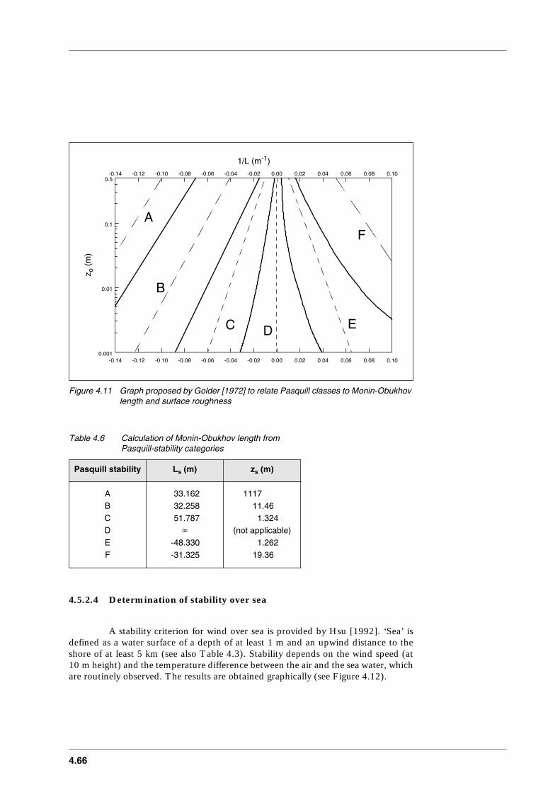
4.66
Figure 4.11 Graph proposed by Golder [1972] to relate Pasquill classes to Monin-Obukhov length and surface roughness
Table 4.6 Calculation of Monin-Obukhov length fromPasquill-stability categories
4.5.2.4 Determination of stability over sea
A stability criterion for wind over sea is provided by Hsu [1992]. ‘Sea’ isdefined as a water surface of a depth of at least 1 m and an upwind distance to theshore of at least 5 km (see also Table 4.3). Stability depends on the wind speed (at10 m height) and the temperature difference between the air and the sea water, whichare routinely observed. The results are obtained graphically (see Figure 4.12).
Pasquill stability L s (m) z s (m)
A 33.162 1117B 32.258 11.46C 51.787 1.324D
∞
(not applicable)E -48.330 1.262F -31.325 19.36
-0.14 -0.12 -0.10 -0.08 -0.06 -0.04 -0.02 0.00 0.02 0.04 0.06 0.08 0.10
-0.14 -0.12 -0.10 -0.08 -0.06 -0.04 -0.02 0.00 0.02 0.04 0.06 0.08 0.10
1/L (m-1)
0.001
0.01
0.1
0.5
A
B
C D E
F
z o (
m)

CPR 14EChapter 4 of the ‘Yellow Book’
4.67
Figure 4.12 Graph proposed by Hsu [1992] to relate Pasquill stability classes and Monin-Obukhov length over sea to the temperature difference between the air and the sea water
4.5.2.5 Mixing height
Mixing height h
i
depends on stability. The recommendations for mixing height are
summarised in Table 4.7. Use needs to be made of the so-called Coriolis parameterf, defined as:
with
Ω
the earth’s rotation (7.27 . 10
-5
s
-1
) and
ϕ
the latitude of position on earth(about 51˚ for The Netherlands).
Also the friction velocity u
*
and Monin-Obukhov length L need to be known. Themixing height is then given by Table 4.7.
-12 -10 -8 -6 -4 -2 0 2 4 6 8 10 12
Temperature difference Tair - Tsea (K)
0
2
4
6
8
10
12
14
1/L=-0.04
DE
C
B F1/L=-0.1
1/L=0.04
1/L=0.1
Win
d sp
eed
at 1
0 m
hei
ght (
m/s
)
f 2 Ω sin ϕ = (4.48)(s -1 )
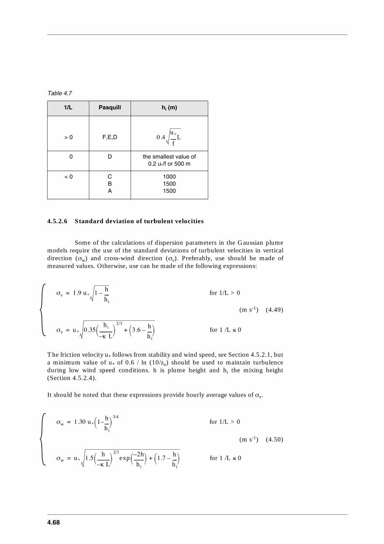
4.68
Table 4.7
4.5.2.6 Standard deviation of turbulent velocities
Some of the calculations of dispersion parameters in the Gaussian plumemodels require the use of the standard deviations of turbulent velocities in verticaldirection (
σ
w
) and cross-wind direction (
σ
v
). Preferably, use should be made ofmeasured values. Otherwise, use can be made of the following expressions:
The friction velocity u
*
follows from stability and wind speed, see Section 4.5.2.1, but
a minimum value of u * of 0.6 / ln (10/z o ) should be used to maintain turbulenceduring low wind speed conditions. h is plume height and h
i
the mixing height
(Section 4.5.2.4).
It should be noted that these expressions provide hourly average values of
σ
v
.
1/L Pasquill h
i
(m)
> 0 F,E,D
0 D the smallest value of0.2 u
*
/f or 500 m
< 0 CBA
100015001500
0.4u*
f-----L
σv 1.9 u * 1 h
h
i
---- –= for 1/L > 0
σv u* 0.35hi
κ– L-----------
2/3
3.6
h
h i ----
–
+=
(4.49)
for 1 /L
≤
0
(m s
-1
)
σw 1.30 u * 1 h
h
i
---- –
3/4 = for 1/L > 0
σw u* 1.5h
κ L– -----------
2/3
exp
2
h
–
h i ---------
1.7
h
h i ----
–
+=
for 1 /L ≤ 0
(4.50)(m s
-1
)
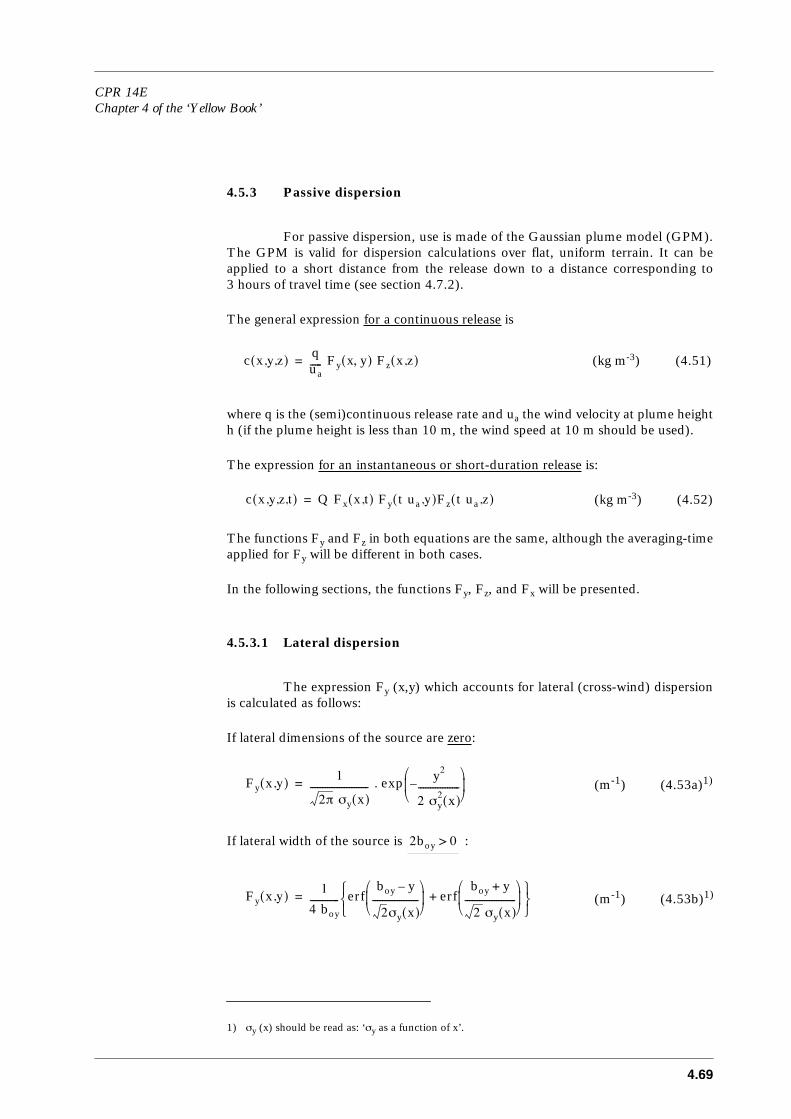
CPR 14EChapter 4 of the ‘Yellow Book’
4.69
4.5.3 Passive dispersion
For passive dispersion, use is made of the Gaussian plume model (GPM).The GPM is valid for dispersion calculations over flat, uniform terrain. It can beapplied to a short distance from the release down to a distance corresponding to3 hours of travel time (see section 4.7.2).
The general expression for a continuous release is
where q is the (semi)continuous release rate and u
a
the wind velocity at plume heighth (if the plume height is less than 10 m, the wind speed at 10 m should be used).
The expression for an instantaneous or short-duration release is:
The functions F
y
and F
z
in both equations are the same, although the averaging-timeapplied for F
y
will be different in both cases.
In the following sections, the functions F
y
, F
z
, and F
x
will be presented.
4.5.3.1 Lateral dispersion
The expression F
y
(x,y) which accounts for lateral (cross-wind) dispersionis calculated as follows:
If lateral dimensions of the source are zero:
If lateral width of the source is :
1)
σ
y
(x) should be read as: ‘
σ
y
as a function of x’.
c x,y,z( )qua----- F y x y ,( ) F z x ,z ( ) = (4.51)(kg m -3 )
c x,y,z,t( ) Q F x x ,t ( ) F y t u a ,y ( ) F z t u a ,z ( ) = (4.52)(kg m -3 )
Fy x,y( )1
2π σ y x ( ) ------------------------ . exp y
2
2 σ y
2 x ( ) -----------------
–
=
(4.53a)
1)
(m
-1
)
2boy > 0
Fy x,y( )1
4 b oy ------------ erf
b
oy
y
–
2 σ y
x ( ) -------------------
erf
b
oy
y
+
2 σ y x ( ) ---------------------
+
=
(4.53b)
1)
(m
-1
)
4.70
The error function erf(x) is defined as erf(x) = .Numerical approximate solutions can be found for instance in Press et al. [1986]. Anreasonable analytical approximation is given by
4.5.3.2 Vertical dispersion
The expression F
z
(x,z) which accounts for vertical dispersion is calculatedas follows:
If vertical dimensions of the source are zero and if
If the vertical dimension of the source is and
If
1)
σ
z
(x) should be read as: ‘
σ
z
as a function of x’.
2/ π -t2( )exp tdox∫
erf x( )x
x -------- 1 e
4x
2
π--------–
–⋅≈
σz x( ) < 0.6 . h i 1 h /h i – :
Fz x,z( )1
2π σ z x ( ) ------------------------ . exp
z h
–
( )
2
2 σ z
2 x ( )
-----------------
–
exp
z h
+
( )
2
2 σ z 2 x ( )
-----------------
–
+
=
(4.57a)
1)
(m
-1
)
2.boz > 0
σz x( ) ≤ 0.6 h i 1 h h i ⁄ – :
Fz x,z( )1
4 b oz ------------ erf
b
oz
z
–
h
+
2 σ z x ( ) ------------------------
erf
b
oz
z h
–+
2 σ z x ( ) ------------------------
+ +=
+ erfb
oz
z
–
h
–
2 σ z x ( ) -----------------------
erf
b
oz
z h
+ +
2 σ z x ( ) ------------------------
+
(4.57b)
1)
(m
-1
)
0.6 h i 1 h /h i – < σ z x ( )≤ 1.6 h i :
Fz x,z( )1
2π σ z x ( ) ------------------------ exp
2
h
i
h
–
z
–
( )
2
2 σ z 2 x ( )
------------------------------
–
exp
2
h
i
h
–
z
+
( )
2 σ z 2 x ( )
----------------------------
–
2
+
=
+ exp 2
h
i
h z
–+
( )
2
2 σ z
2 x ( ) ------------------------------
–
exp
2
h
i
h z
+ +
( )
2
2 σ z 2 x ( )
-------------------------------
–
+
(4.57c)
1)
(m
-1
)
+ exp z h – ( )
2
2 σ z
2 x ( )
-----------------
–
exp
z h
+
( )
2
2 σ z 2 x ( )
-----------------
–
+

CPR 14EChapter 4 of the ‘Yellow Book’
4.71
If :
Formula (4.57c) accounts for reflection of plume material at the mixing height,formula (4.57d) assumes the plume material to be uniformly distributed in the mixedlayer. In these cases the effects of finite source dimensions are negligible.
4.5.3.3 Along-wind dispersion
For
instantaneous releases
at time t = 0, the term F
x
which accounts foralong-wind dispersion is calculated as follows:
If longitudinal dimensions of the source are zero:
If longitudinal dimension of the source is :
(here, t is time since release)
For
short duration releases
with total emission Q during a release time from t = 0to t = t
r
, Bianconi and Tamponi [1993] derived the following approximate solution(the solution is exact in case the dispersion parameters are proportional to the squareroot of diffusion constant times travel time):
for :
1)
σ
z
(x) should be read as: ‘
σ
z
as a function of x’.2) Here
σ
x
(u
a
t) should be read as: ‘
σ
x
as a function of u
a
.t’3) Here
σ
x
(x) should be read as: ‘
σ
x
as a function of x’
σz x( ) > 1.6 h i
Fz x,z( ) 1
hi----= (4.57d)1)(m-1)
Fx x,t( )1
2π σ x u a t ( ) ----------------------------- exp
x u
a t
–
( )
2
2
σ
x
2
u
a
t
( )
---------------------- –
= (4.59a) 2) (m -1 )
2 b ox > 0
Fx x,t( )1
4box---------- erf
box x– uat+
2 σ x u a t ( ) ----------------------------
erf
b
ox
x u
a
–
t
+
2 σ x u a t ( ) --------------------------
+
=
(4.59b)
2)
(m
-1
)
0 < t < t r
Fx x,t( )1
2 u a t r ------------- erf x
2 σ x x ( ) ---------------------
–
=
erfx uat–
2 σ x x ( ) ---------------------
(4.60a)
3)
(m
-1
)

4.72
For :
4.5.3.4 Dispersion parameters
Continuous source
1. Practical formulae for
σ
y
and
σ
z
For practical calculations
σ
y
and
σ
z
are approximated as follows [Commissie TNO,1976]:
(adjusted for 100 to 10
4
m)
For a,b,c and d the values according to Table 4.8 are applicable:
Notes:
1.
σ
y
to be taken as 10-minutes average
2.
σ
z
for z
0
= 0.1 m and h < 20 m
3.
x,
σ
y
,
σ
z
in meters
Nb: If it is necessary to consider distances smaller than 100 meters in thecalculation, it is best to interpolate linearly between 0 and the value of
σ
at 100meters.
Table 4.8 Parameters for the calculation of
σ
y
and
σ
z
, adjusted according to ref. 1,2,3.
a b c d
Very unstable (A) 0.527 0.865 0.28 0.90
Unstable (B) 0.371 0.866 0.23 0.85
Slightly unstable (C) 0.209 0.897 0.22 0.80
Neutral (D) 0.128 0.905 0.20 0.76
Stable (E) 0.098 0.902 0.15 0.73
Very stable (F) 0.065 0.902 0.12 0.67
t tr≥
erfx uat–
2 σ x u a t ( ) --------------------------
(4.60b)(m
-1
)
Fx x,t( )1
2 u a t r ------------- erf
x u
a
t t
r
–
( )
–
2 σ x u a t ( ) ----------------------------
–
=
σy x( ) a xb⋅=
σz x( ) c xd⋅=

CPR 14EChapter 4 of the ‘Yellow Book’
4.73
2. Correction for the roughness length z
0
Reference [Pasquill and Smith, 1983] gives a method for taking into account theroughness of the earth’s surface and, in particular, the effect of it on the dispersion inthe z-direction.
The roughness also includes overgrowth, cultivations and building. In Table 4.9;
σ
z
is given for z
0
= 0.1 m. For other roughness lengths a correction factor according toref. [Pasquill and Smith, 1983] is used. However, the calculation is made with the aidof a formula according to ref. [Commissie TNO, 1976]:
Table 4.9 gives some representative values for z
0
.
Since C
z0
depends on x, it will be easier and even necessary, for most applications, tocalculate, for a given value of z
0
, new values for c and d, so that with equation:
σ
z
(x)
= c . x
d
one can immediately obtain the corrected values of
σ
z
(see Table 4.9).
Nb: All of the values can be approximated by the use of the two equations below:
Flat land (f.i. polder land with few trees) z
0
= ca. 0.03 m
Farm land (f.i. airfield, aqricultural land, polder with many trees) z
0
= ca. 0.10 m
Cultivated land (f.i. glass-house land, open area with much overgrowth, scattered houses)
z
0
= ca. 0.30 m
Residential land (f.i. area with densely located but low buildings, wooded area, industrial area with obstacles which are not to high)
z
0
= ca. 1.0 m
Urban land (f.i. a big city with high buildings, industrial area with high obstacles)
z
0
= ca. 3.0 m
Table 4.9 Values of c
'
and d
'
for various values of z
0
.
z
0
= 0.03 m z
0
= 0.1 m z
0
= 0.3 m z
0
= 1 m z
0
= 3 m
Very unstable (A) 0.193 0.932 0.28 0.90 0.383 0.873 0.550 0.842 0.760 0.814
Unstable (B) 0.160 0.881 0.23 0.85 0.317 0.822 0.455 0.792 0.631 0.763
Slightly unstable (C) 0.155 0.830 0.22 0.80 0.308 0.771 0.441 0.740 0.612 0.712
Neutral (D) 0.139 0.791 0.20 0.76 0.276 0.732 0.395 0.701 0.548 0.673
Stable (E) 0.104 0.761 0.15 0.73 0.207 0.702 0.296 0.671 0.411 0.643
Very stable (F) 0.083 0.701 0.12 0.67 0.164 0.642 0.236 0.611 0.327 0.583
Cz010 z0⋅( )0.53 x
0.22–⋅=
σz x( ) Cz0c x⋅ d⋅=
c' d' c' d' c' d' c' d' c' d'
c' c 1.9810 z0⋅( )log
⋅=
d' d 0.059– 10 z0⋅( )log⋅=

4.74
The new values of c and d will be then called and in the text, whereby thefollowing applies to
σ
z
:
3. Correction for the mean time of a measurement
If we take a snap shot of a smoke plume we see a band winding erratically (as thehatched part in Figure 4.13). If, however, we were to take an exposure lasting, let ussay, 10 minutes, much of the effort of the winding (the ‘meandering’) would be“averaged out” and we would see a much broader and more regular plume.
Figure 4.13 Schematic representation of a plume. The hatched part is a snap-shot, the wider contour an average over 10 minutes.
This effort influences measurements and the quantity which a person breathes-in. Ifa short-duration measurement is taken in an instantaneous position of the plume, ahigh concentration is registered. If, however, an average value is determined at thesame location over a period of, for instance, 10 minutes or an hour, the concentrationwill be substantially lower. This can be approximately brought into the calculation byintroducing a correction factor C
t'
as follows:
Nb: This correction is consequently only applicable to
σ
y
.σy cannot, however, be smaller than the value for an instantaneous source (see next section). The factor Ct' has a minimum value of about 0.5.
c' d'
σz x( ) c' xd'⋅=
Ct't'
600--------
0.2
t' in seconds( )=
σy x( ) Ct' a xb⋅ ⋅=

CPR 14EChapter 4 of the ‘Yellow Book’
4.75
Instantaneous source
4. Practical formulae for σxI, σyI and σzI
σxI, σyI and σzI are described by the equations:
The data in the literature for these variables are clearly scarcer than those forcontinuous sources. Values for σxI, determined partly theoretically, partlyexperimentally, are given in the references [Beals, 1971], [Drivas and Shair, 1974],[Saffman, 1962], [Tyldesley and Wallington, 1965] and [Chatwin, 1968]. In view ofthe limited nature of the data, it is all put together by taking the same σxI for allstability classes (= 0.13·x). The values of σyI are in the initial stage based on reference[Slade, 1968], with a small adjustment in order to avoid discrepancies with the valuefor σy in case of an continuous source. The value of σzI is chosen equal to the one ofa continuous source, since the correction for the average-time hardly plays a role inthis case and because of the fact that close to the ground the vertical “meandering” isrepressed by the presence of the ground surface. In reference [Hanna, Briggs andHosker, 1982] a comparison is made between continuous and instantaneous sources.There it is found that the standard radial deviation of the concentration (σ) of aninstantaneous cloud is proportional to the age of the cloud increased by the power of3/2. For large times σ (instantaneous) approaches the value of σ (continuous), so thatthe values of the sigmas previously described and practical to apply can be used.
Consequently, we arrive at the following values for the constants:
eI = 0.13 fI = 1
aI = a/2 bI = b
cI = c dI = 1
The correction factor Ct' is obviously hereby not applicable. The correction factor Cz0for σz is applicable. The values obtained with the help of the above constants areapplicable at ground level. For σxI, in particular, it must be considered that σxI isstrongly dependent on the height of the source since it is primarily influenced by theincrease of the wind with the height. Also hereby it is more practical, in most cases,for the z0 from which we want to initiate our calculations, to determine first thecorrected values of cI and dI.
σxI x( ) eI xfI⋅=
σyI x( ) aI xbI⋅=
σzI x( ) cI xdI⋅=

4.76
4.5.3.5 Sources with finite dimensions
In Sections 4.5.3.1 and 4.5.3.2 solutions are presented for situations inwhich a continuous source has merely cross-wind or vertical dimensions.
For merely along-wind dimensions 2 box, the GPM-solution (Gaussian PlumeModel) for a continuous release is:
It appears that already at a short distance the effect of box becomes small.
For line sources which are not oblique or parallel to the wind, the line source shouldbe discretised in a large number of point sources.
For area sources with arbitrary shapes, the area can be divided into a number of cross-wind line sources.
4.5.3.6 Sources with time-dependent release rates
A source for which the release rate varies with time can be dealt with byintegrating a series of instantaneous releases with a released mass q(t)dt over the timeof release:
4.5.3.7 Considerations with respect to semi-continuous or time-dependent releases
At a short distance from a release which has a constant release rate q over afinite release time tr, one will observe for a certain time a plume as if it were acontinuous release with the same release rate q.In contrast, at a large distance, even a release over a fairly long period will be observedas a single ‘puff’.Although the expressions (4.60a,b) and (4.63) are correct and applicable to alldistances, one may simplify the calculations, as in the former ‘Yellow Book’, by usingthe formula (4.51) for continuous sources up to a down-wind distance where
σx(x) < 0.13 ua tr (m) (4.64a),
c x,y,z( )q
2boxua---------------- F y x
' ,y ( ) F z x ' ,z ( ) dx
'
x b
ox
–
( )
x b
ox
+
( )
∫ = (4.62)(kg m -3 )
c x,y,z,t( ) q t'( )Fx x,t t'–( )Fy t t'–( )ua,y( ) Fz t t'–( )ua,z( )dt'
0
∞
∫=
(kg m-3) (4.63)

CPR 14EChapter 4 of the ‘Yellow Book’
4.77
whereas formula (4.52) for pure instantaneous releases may be used for distancesbeyond where
σ
x
(x) > 1.3 u
a
t
r
(m) (4.64b)
These simplifications reduce the complexity and time consumption of thecalculations but introduce considerable continuity problems for C (x, y, z, t) in thedown-wind axis (0 < x <
∞
).
4.5.3.8 Calculation of the total mass of contaminant between Lower and Upper Flammability Limit
In order to assess the impact of delayed ignition of a cloud of inflammablematerial, it is necessary to calculate the total mass of inflammable material betweenLFL and UFL.
The general methodology for any type of source or release is as follows:
where the function f (x,y,z,t) is defined as follows:
f (x,y,z,t) = c (x,y,z,t) if LFL < c (x,y,z,t) < UFL
f (x,y,z,t) = 0 elsewhere.
(For continuous releases, the dependency on time vanishes.)Here, the concentration has to be calculated by the appropriate representation,depending release mode and source dimensions. For these calculations the lateraldispersion parameter
σ
y
(x) for instantaneous plume cross-sections must be used!
In general, this integral needs to be solved numerically, in discretised form. Theevaluation of the integral of (4.65) starts in practice by finding the maximum LFL-distance x
lfl
, the maximum cloud width to LFL, y
lfl
, and the maximum cloud heightto LFL, z
lfl
. In order to obtain practical values for these upper boundaries forintegration, some methods will be provided to estimate the contour to the LFL, byuse of approximate analytical solutions.
For a continuous point source at ground level, the down-wind distance to the LFLcan be calculated as:
Qex t( ) f x ,y,z,t ( ) dxdydz ,
0
z
lfl
∫
-
y
lfl
y
lfl
∫
0
x
lfl
∫ = (4.65)(kg)
xlfl ,groundq
π 0.3 σ v f z 1 z o L ,( ) c lfl ---------------------------------------------------
1
f
z
2
L
( )
1+
-----------------------
=
(4.66a)(m)

4.78
Here c
lfl
denotes the LFL concentration, f
z1
(z
o
,L) and f
z2
(L) follow from (4.58).
It should be noted that for an elevated plume which has not yet touched the ground,the LFL at centre-line is reached at a shorter distance:
For plumes which have touched the ground, x
lfl
will be between x
lfl,elevated
andx
lfl,ground
.
Note that we consider the plume to touch the ground if 2
×
σ
z
> h.
The cross-wind distance to LFL at the ground can be calculated for elevated plumesand plumes at the ground by:
where c(x,0,0) is the concentration at ground level below the plume centre-line.
In the previous approximations of LFL-contours, one may include initial sourcedimensions by means of a virtual source distance. The virtual source distances x
vy
andx
vz
follow from the implicit relations:
A conservative estimate for x
lfl
can be obtained by substracting the smaller value ofx
vy
or x
vz
from x
lfl,ground
or x
lfl,elevated
. y
lfl
(x) can be obtained by using
σ
y
(x+x
vy
) and
σ
z
(x+x
vz
) instead of
σ
y
(x) and
σ
z
(x) in (4.67) (including in the calculation ofc(x,0,0)).
For continuous point sources, the mass Q
ex
between UFL and LFL can be obtainedfrom an approximate analytical solution:
x
ufl
can be calculated similar as x
lfl
.
1)
σ
y
(x) should be read as: ‘
σ
y
as a function of x’.
xlfl ,elevated xlfl ,ground1
2--
1
fz2 L( )---------------
= (4.66b)(m)
ylfl x( ) σy x( ) 2 ln c x ,0,0 ( ) c
lfl
------------------ = (4.67) 1) (m)
σy xvy( )boy
2.15--------- , σ z x vz ( )
b
oz 2.15
--------- == (4.68)
Qex
q--------
fz2 L( ) 1+
fz2 L( ) 2+----------------------
x lfl
x
ufl –
u
a
-------------------- = (4.69)(s)
CPR 14EChapter 4 of the ‘Yellow Book’
4.79
For sources with initial dimension, but for which x
vy
∼
x
vz
= x
v
, this solution is:
Note that Q
ex
/q = 0 if x
lfl
= 0, which will be the case when the initial concentration islower than x
lfl
.
4.5.4 Models for jets, plumes and plume rise
4.5.4.1 The free turbulent jet model
The aim of this section is to explain the jet model of Chen and Rodi [1980],which has been selected for the description of gas releases in a uniform quiescentatmosphere. The source is axially symmetric, with a radius b
o
and a uniform outflowvelocity u
o
in vertical direction. The model is valid for gases which can beapproximated to be incompressible, i.e. the release velocity should be less than aboutone-third of the speed of sound under ambient pressure. In cases where buoyancy canbe neglected, the requirement on the initial direction of the release can be omitted.The formulation of flow development is based on the self-preserving properties of jetreleases, which is discussed in Section 4.3.4. In a self-preserving flow, simpleexpressions exist for the centre-line velocity and concentration of the releasedchemical compound. Chen and Rodi determine common values for the empiricalconstants in the expressions. They define empirical conditions under which a jetmodel is applicable, and give expressions for the distribution functions of physicalquantities in the lateral cross-sections of the flow (i.e., perpendicular to the mean flowaxis).The dynamical similarity of positively buoyant jets is a good approximation as long as
where Fr is the (densimetric) Froude number,
ρ
o
and
ρ
a
are the densities ofrespectively the initial chemical compound and air, b
o
is the radius of the source ands is the axial distance to the hypothetical point source with the same flowcharacteristics as the real source. The Froude number was already defined in Section4.3.4 as a measure for the relative importance of initial momentum and weight deficit.
Qex
q--------
1
ua-----
fz2 L( ) 1+( )
fz2 L( ) 2+--------------------------- x lfl x ufl – ( )
x
v
f
z
2
L
( )
2+
( )
f
z
2
L
( )
2+
---------------------- 1
x
ufl
f
z
2
L
( )
1+
( )
---------------------- 1 x
lflf
z
2
L
( )
1+
( )
---------------------- –
–
=
if x
ufl
> 0
Qex
q--------1ua-----=
fz2 L( ) 1+( )
fz2 L( ) 2+--------------------------- x lfl x v
x
v
f
z
2
L
( )
2+
( )
f
z
2
L
( )
2+
( )
x
lfl
f
z
2
L
( )
1+
( )
-------------------------------------------------- +–
(4.70)
if x ufl = 0
(s)
s 0.5 b⋅ o Fr ρ o / ρ a ( ) 1/4 < (4.71),(m)
Frρo
ρa ρo–------------------
u
o
2
2
b
o
g
----------- = (4.72).(-)
4.80
Here u
o
is the exit velocity from the source.
The condition (4.71) implies that the model is only usable in cases in which inertialforces dominate over buoyant forces.The no wind condition of the free jet model applied to vertical or cross-wind releasesis equivalent to assuming that the centre-line velocity is much larger than the ambientwind velocity, typically by a factor of 10. In other situations, simple expressions forthe flow quantities do not exist, and calculations have to be done with plume riseformulae (see Section 4.5.4.2), the Gaussian plume model (Section 4.5.3) andintegral models like the SLAB computer model (Section 4.5.5.2).
The distribution functions, or profiles, are functions only of the nondimensionalcross-flow coordinate y/s. The experimental observations show that the velocity andconcentration profiles are approximately Gaussian after the potential core at adistance s
s
(see Table 4.10) has disappeared:
u(y/s) / u
c
(s) = exp(-C
yu
(y/s)
2
) (-) (4.73),
c(y/s) / c
c
(s) = exp(-C
yc
(y/s)
2
) (-) (4.74).
u
c
(s) and c
c
(s) are the centre-line values, and C
yu
and C
yc
are empirical constants thatdetermine the profile width. The concentration of the chemical compound is definedin parts per unit volume relative to atmospheric level, i.e. it is the difference betweenthe local value and the value in air. The width constants turn out to be different forjets and plumes.
Non-buoyant jets
Non-buoyant jets are defined as releases of a chemical compound whose density
ρ
o
isequal to the density
ρ
a
of ambient air. The collection of experimental data sets in thereview of Chen and Rodi consists mainly of this type of release. Some typical aspectswere observed in the data sets:
–
In most of the experiments, the locations of the real (circular) source and thevirtual point source of the model do not coincide, i.e. the real source is located ata distance +(s
o
). A good approximation is to take s
o
= 0.
–
In lateral direction, the concentration profiles are broader than the correspondingvelocity profiles.
–
Close to the source, the potential core is still visible in the jet profile. The distances
s
from the origin to the region of established flow can be derived from thelocation, where the jet profiles in lateral direction become Gaussian and (4.73)and (4.74) become valid. A good approximation is to take S
s
/b
o
= 25.The jet flow in the region of established flow is described by the set of equations
u
c
(s)/u
o
= C
u
b
o
/s (-) (4.75).
c
c
(s)/c
o
= C
c
b
o
/s (-) (4.76).
c
o
is the concentration of the initial chemical compound. A number of empiricalconstants occur in the model: C
u
, C
c
, C
yu
, C
yc
, s
o
and s
s
, and their values are given inTable 4.10 for the non-buoyant jet model of Chen and Rodi. The values for C
u ,C
c ,
C
yu
and C
yc
are recommendations, whereas for s
o
and s
s
also the range of observedvalues is indicated.

CPR 14EChapter 4 of the ‘Yellow Book’
4.81
Buoyant jets
Buoyant jets have an initial density
ρ
o
which is different from the density
ρ
a
ofambient air. The expressions 4.74-4.77 are still valid as long as condition 4.73 issatisfied. The empirical constants C
u
, C
c
, C
yu
and C
yc
can then be obtained from thevalues for a non-buoyant jet in Table 4.10. Chen and Rodi [1980] suggest in theirmonograph to correct the constants for density effects:
A vertical negatively buoyant jet rises to a maximum height s
h
and then falls back onitself. Chen and Rodi give an equation for the height:
Also for negatively buoyant jets the formulae 4.74-4.79 are valid as long as s < s
h
.
Table 4.10 Empirical constants in the non-buoyant jet model of Chen and Rodi [1980]
Zone limits for ignition and explosive contents
The limiting distances for the ignition of a jet release are determined by the upper andlower flammability level of the chemical compound. A conservative estimate of thesafe distance is obtained by equating the concentration on the jet axis to the lowerflammability level c
lfl
. The safe distance s
lfl
for jets and plumes can then be derivedfrom the equation 4.76, and taking into account (4.79):
non-buoyant jet
Cu 6.2Cc 5Cyu 94Cyc 57so/bo 0 (range -6 to 6)ss/bo 25 (range 20 to 30)
Cu'
ρo
ρa----- C u = (-) (4.77)
Cc'
ρa
ρo----- C c = (-) (4.78).
sh 4.11 Fr b o = (4.79).(m)
slf1 min boCc'
co
clfl------ , sh
= (4.80)(m)
4.82
The width of the lower flammability level isocontour can be derived from theequations 4.74, and 4.73. For jets they are given by
Note that the equation is invalid in the region of flow establishment, close to thesource (s < s
s
).The explosive contents of jets and plumes is obtained by integrating over the volumebetween the upper and lower flammability isocontours. The mathematicalformulation for the mass contents of the chemical compound is
Note, that in this paragraph c o , c ufl and c lfl are to be used in parts per unit volume.If c
o
< c
ufl
the last term between the brackets vanishes. If c
o
< c
lfl
then Q
ex
= 0.
4.5.4.2 Models for jets and plumes in ambient wind
This section discusses the model of Hoot, Meroney and Peterka [HMP,1973] for the dispersion of negatively buoyant plumes, and Briggs formulae [1969]regarding positively buoyant plumes. The models describe the plume trajectory, withemphasis on the development in the region of plume rise. The discussion is based onthe one-dimensional integral plume theory, and on the analytical expressions whichare derived from simplified versions of this theory. The basic assumptions of thetheory are explained in Section 4.3.4. The model is valid for gases which can beapproximated to be incompressible, i.e. the release velocity should be less than one-third of the speed of sound under ambient pressure.
The model of Hoot, Meroney and Peterka
Negatively buoyant jets and plumes injected vertically into a cross-wind initially loftto some maximum height, subsequently descend to the ground, impact to the groundwith a nearly circular cross-sectional configuration, and then spread laterally as theydisperse down-wind (see Figure 4.14).
ylfl,jet s( ) s/ Cyc( ) lnbo
s-----Cc
' co
clfl------
= (4.81)(m)
Qex
πρobo3 Cc
'( )3co
6Cyc--------------------------------
co
clfl------
2 co
cufl-------
2
–= (4.82).(kg)
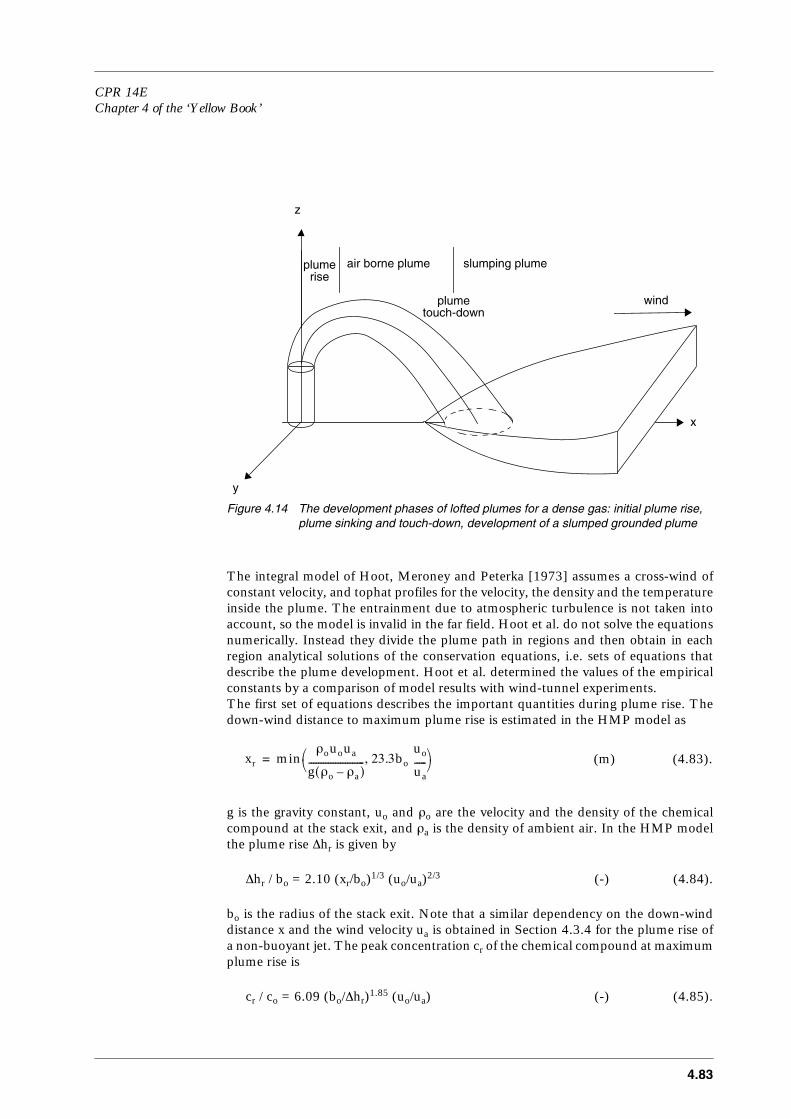
CPR 14EChapter 4 of the ‘Yellow Book’
4.83
Figure 4.14 The development phases of lofted plumes for a dense gas: initial plume rise, plume sinking and touch-down, development of a slumped grounded plume
The integral model of Hoot, Meroney and Peterka [1973] assumes a cross-wind ofconstant velocity, and tophat profiles for the velocity, the density and the temperatureinside the plume. The entrainment due to atmospheric turbulence is not taken intoaccount, so the model is invalid in the far field. Hoot et al. do not solve the equationsnumerically. Instead they divide the plume path in regions and then obtain in eachregion analytical solutions of the conservation equations, i.e. sets of equations thatdescribe the plume development. Hoot et al. determined the values of the empiricalconstants by a comparison of model results with wind-tunnel experiments.The first set of equations describes the important quantities during plume rise. Thedown-wind distance to maximum plume rise is estimated in the HMP model as
g is the gravity constant, u
o
and
ρ
o
are the velocity and the density of the chemicalcompound at the stack exit, and
ρ
a
is the density of ambient air. In the HMP modelthe plume rise
∆
h
r
is given by
∆
h
r
/ b
o
= 2.10 (x
r
/b
o
)1/3 (uo/ua)2/3 (-) (4.84).
bo is the radius of the stack exit. Note that a similar dependency on the down-winddistance x and the wind velocity ua is obtained in Section 4.3.4 for the plume rise ofa non-buoyant jet. The peak concentration cr of the chemical compound at maximumplume rise is
cr / co = 6.09 (bo/∆hr)1.85 (uo/ua) (-) (4.85).
x
z
wind
y
plumerise
air borne plume slumping plume
plumetouch-down
xr minρououa
g ρo ρa–( )----------------------- 23.3bo
uo
ua-----,
= (4.83).(m)
4.84
The second set of equations in the HMP model describes the important quantitiesduring plume touch-down to the ground. The location xg of the maximal groundconcentration is given in the HMP model by
hs is the height of the stack. At touch-down the surface peak concentrations cg are ofthe order
cg / co = 9.4 (bo/(hs + 2∆hr))1.95 (uo/ua) (-) (4.87).
The surface concentration decreases from the touch-down value as the plumematerial is transported down-wind and gradually approaches the behaviour of aground source.
The Briggs formulae for plume riseIn the simplified integral trajectory theory discussed by Davidson [1989] the rise of apositively buoyant plume, neglecting momentum rise, is related to the down-winddistance (x) by a 2/3-power law. Briggs [1969] has derived the empirical constants inthe plume rise relations by measuring plume rises from conventional stacks in calmand windy, thermally stratified atmospheres. The equation for the plume trajectoryaccording to Briggs is
∆hB(x) = 1.60 Fo1/3 x2/3 / ua (m) (4.88).
Here, ua is the wind speed at release height, with a minimum of 10 m.Fo is the buoyancy flux factor, defined as
(m4 s-3) (4.89),
Briggs states that in a neutral or unstable atmosphere (Pasquill-classes A, B, C andD) the plume final rise occurs at
xr = C1 . Fo5/8 if Fo ≤ 55 m4/s3
(m) (4.90)xr = C2 . Fo
2/5 if Fo > 55 m4/s3
Here, C1 = 49 m-3/2 s15/8, and C2 = 119 m-3/5 s6/5.
The plume final rise is obtained by substitution of the equation 4.90 (xr) in equation4.88.
For a release in a stable atmosphere (Pasquill-classes E and F) it is advised to employa relation from the Dutch National Model. The National Model states that full riseoccurs at
xr = C3 ua (m) (4.91).
Here, C3 = 87 s.
xg xr– 0.28 hs 2∆hr+( )3 ∆hr3–( )/bo( )
1/2ρa/ρo( )1/2 xr/bo( )1/2 ua/u0( )=
(4.86).(m)
Fo gbo2 u o 1
ρ
o ρ
a
----- – =

CPR 14EChapter 4 of the ‘Yellow Book’
4.85
Equation 4.91 is valid as long as the vertical temperature gradient at heights between10 and 200 m in the atmosphere is on average -0.0065 K/m, which corresponds to atemperature gradient as observed under neutral conditions (Pasquill-class D) in TheNetherlands.
For low wind velocities in a neutral or unstable atmosphere, the calculation of theplume rise with the equations 4.88-4.90 gives values which are larger than themeasured values. Therefore a rule of thumb has been set, stating that in neutral orunstable conditions the calculated plume rise must not exceed the plume risecalculated for stable conditions. In cases where the rule is violated, the equation 4.91for stable conditions should be applied.
Briggs [1969] has also derived expressions for plume rise dominated by momentumforces, under conditions of neutral atmospheric stability. They are:
∆
h
M
= 6 b
o
u
o
/ u
a
(m) (4.92).
and
x
r
= 23.3 b
o
u
o
/ u
a
In cases where both the initial momentum and buoyancy contribute to the final plumerise, it is calculated according to
Trajectory and dilution predictions from simple integral plume theory
The flow diagram in Section 4.5.1 shows that plume rise formulae are used to providethe initial conditions for more complex dispersion models. In some cases it will benecessary to predict the concentration distribution of the release during plume rise.This can be calculated in a 3-step procedure with the simple model discussed byDavidson [1989].
First, the plume trajectory is calculated for all down-wind distances x during plumerise, by means of equation 4.84 for negatively buoyant jets and by means of equations4.92 (for plume rise
∆
h
M
due to momentum), 4.88 and 4.93 for neutral or positivelybuoyant jets. The local height h(x) - h
s
is obtained from these equations by replacingx
r
by x.
The radius at other down-wind distances can be calculated by:
Finally, for a concentration distribution with a tophat shape the cross-sectionalaveraged concentration can be calculated by:
c(x)/c
o
= (b
o
/b(x))
2
(u
o
/u
a
) (-) (4.95).
(Note the similarity of the model equation 4.95 with the empirical equations 4.85 and4.88 for the peak concentrations in the HMP model).
∆hr ∆hB3 ∆hM
3+( )1/3
= (4.93).(m)
b x( ) bo
ρouo
ρaua----------- 0.41 h x( ) hs–( )+= (4.94).(m)

4.86
The total mass of inflammable material can be calculated by the general expression4.65.
4.5.5 Dense gas dispersion models
The purpose of this section is 3-fold:1. To give a scientific description of 2 models for dense gas dispersion, i.e. the
Workbook of Britter and McQuaid [1988], and the SLAB computer model[Ermak, 1990]. The description treats the scientific aspects in detail, or refers tothe open literature in cases where such a treatment would be too extensive.
2. To indicate the sensitivity, robustness, reliability and restrictions of the algorithmsin the 2 models.
3. To provide the user with the same information in order to allow for an effectiveuse of the model, including the preparation of input data and interpretation of themodel output.
In other words, the contents of the section is an assessment of the algorithms in themodels from a physical point of view, and a discussion of the connection between thein/output parameters of the models and the physical concepts in dense gasatmospheric dispersion.The 2 models are developed for use in different situations:
–
The Britter and McQuaid Workbook contains a set of nomograms whichrepresent the concentration decay in releases from a continuous point source andan instantaneous cubic source, as a function of down-wind distance. It is usefulfor calculations with an indicative purpose.
–
The SLAB computer code should be applied in more advanced dense gasdispersion studies. It describes the concentration in a cloud or plume by solving a1-dimensional set of conservation equations for mass, chemical compoundconcentration, energy and the 3 components of momentum. The source can be ahorizontal or vertical jet, a steady state surface area source, or an instantaneousrelease.
4.5.5.1 The Britter and McQuaid model
The model of Britter and McQuaid consists of empirical correlationsbetween a set of independent variables that determine the gross properties of thedense gas dispersion process. The correlations are presented in an extensiveWorkbook which has been written by Britter and McQuaid [1988] in order to enablenon-specialists to prepare estimates of the dispersion of pollutant dense gasemissions. The simplicity of the model imposes restrictions on its applicability. Theprimary aim of the model is to enable estimates of:
–
average concentration levels along the plume axis, for continuous releases, and
–
maximum concentration levels along the down-wind cloud path, forinstantaneous releases.
In addition, Britter and McQuaid give rules of thumb to estimate isoconcentrationcontours.The correlations are based on the method of dimensional analysis which has beenpresented in Section 4.3.5.1. It is shown there that the dimensional analysis gives themost compact results when the continuous and instantaneous releases are treatedseparately. This approach is also followed in the Britter and McQuaid (BM) model.

CPR 14EChapter 4 of the ‘Yellow Book’
4.87
Figure 4.15 Nomograms for instantaneous releases, according to the Workbook of Britter and McQuaid. Note: the curves correspond to the indicated values of c
max
/c
o
.
Correlations for instantaneous releases
The BM model consists of a collection of curves for down-wind maximumconcentrations c
max
/c
o
in the range between 0.001 and 0.1, which provide thefunctional behaviour of x/V
o1/3
versus u
a2
/(g
o'
V
o1/3
):
The symbols in equation 4.96 have already been defined in Section 4.3.5.1.Figure 4.15 is a graphical presentation of the curves, or nomograms, in the BMmodel. The nomograms were derived from widely-accepted field test data (usuallyreferred to as ‘Porton Down’ and ‘Thorney Island’) and from windtunnel data (seethe Workbook of Britter and McQuaid, for more detailed information).
go' Vo
1/3
ua2--------------
1/2
x/Vo
1/3
(-)
(-)
x / V o 1/3 f i g
o ' V o
1/3 / u a 2 ( )[ ] = (4.96).(-)

4.88
It is noted that the dimensionless parameter u
a2
/(g
o'
V
o1/3
) is transformed in equation4.96 so that its range of values for the used field and laboratory experimental data isof the order of unity: 0.7 < < 10.The reference wind velocity u
a
is taken at a height of 10 m. Concentration values areintended to be valid for the ensemble-average of the maximum of short-time (0.6s)mean concentrations. Here ‘ensemble-average’ means that the fluctuations, whichoccur between successive experiments due to changes in the atmospheric conditionsand in the in-cloud conditions, are averaged out.
As already mentioned in the introduction, the BM cloud model was developed inorder to calculate the down-wind maximum concentration values on the path of thecloud centre. This enables a conservative estimate to be made of the safe distance forignition or intoxication in all directions. The Workbook of Britter and McQuaiddescribes another procedure in order to determine the safe distances (in other words,the isocontours) with greater precision. It consists of 3 steps:
Figure 4.16 Approximations for isoconcentration contours of instantaneous releases, according to the Workbook of Britter and McQuaid
1. Calculate the down-wind distance x to the safe concentration level with thenomograms of the BM cloud model;
2. Calculate the arrival time t of the cloud at x from the relation
x = 0.4u
a
t + b(t) (m) (4.97),
where 0.4u
a
is an empirical estimate of the advection velocity, and b is the cloud
radius. It is given by
go' Vo
1/3/ua2( )
b
bo
x(t)x
b x( ) bo2 3 x/ua( ) go
' Vo+=
wind
y
b t( ) bo2 1.2t go
' V o ( ) += (4.98).(m)
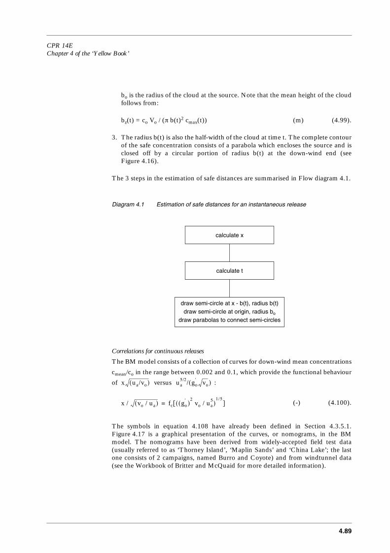
CPR 14EChapter 4 of the ‘Yellow Book’
4.89
b
o
is the radius of the cloud at the source. Note that the mean height of the cloudfollows from:
b
z
(t) = c
o
V
o
/ (
π
b(t)
2
c
max
(t)) (m) (4.99).
3. The radius b(t) is also the half-width of the cloud at time t. The complete contourof the safe concentration consists of a parabola which encloses the source and isclosed off by a circular portion of radius b(t) at the down-wind end (seeFigure 4.16).
The 3 steps in the estimation of safe distances are summarised in Flow diagram 4.1.
Diagram 4.1 Estimation of safe distances for an instantaneous release
Correlations for continuous releases
The BM model consists of a collection of curves for down-wind mean concentrations
c
mean
/c
o
in the range between 0.002 and 0.1, which provide the functional behaviour
of versus :
The symbols in equation 4.108 have already been defined in Section 4.3.5.1.Figure 4.17 is a graphical presentation of the curves, or nomograms, in the BMmodel. The nomograms have been derived from widely-accepted field test data(usually referred to as ‘Thorney Island’, ‘Maplin Sands’ and ‘China Lake’; the lastone consists of 2 campaigns, named Burro and Coyote) and from windtunnel data(see the Workbook of Britter and McQuaid for more detailed information).
calculate x
calculate t
draw semi-circle at x - b(t), radius b(t)draw semi-circle at origin, radius bo
draw parabolas to connect semi-circles
x ua/vo( ) ua5/2/ go
' vo( )
x / v o / u a ( ) f c g o ' ( )
2 v o / u a
5 ( ) 1/5
[ ] = (4.100).(-)

4.90
Figure 4.17 Nomograms for continuous releases, according to the Workbook of Britter and McQuaid. Note: the curves correspond to the indicated values of c
mean
/c
o
.
It is noted that the dimensionless parameter is transformed in equation4.100 so that its range of values for the used field and laboratory experimental data isof the order of unity: 0 < ((g o
' )
2 v o / u a
5 )
1/5 < 4. The reference wind velocity u a is taken
at a height of 10 m. Concentration values are long-time (order of 10 min) averages,so greater concentrations are possible over short times due to fluctuations inconcentration. Britter and McQuaid suggest that short-duration averagedconcentrations can be a factor 1.6 higher than C
mean
.A conservative estimate of the safe distance for ignition or intoxication in alldirections is obtained by calculating the down-wind mean concentration values onthe plume axis. The Workbook of Britter and McQuaid describes another procedurein order to determine the safe distances with greater precision. It describes the plumeby means of empirical expressions for the cross-wind plume area, and consists of 3steps:
go'2vo
ua5
-----------
1/5
x/vo
ua-----
1/2
(-)
(-)
ua5/2/ go
' vo( )

CPR 14EChapter 4 of the ‘Yellow Book’
4.91
Figure 4.18 Approximations for isoconcentration contours of continuous releases, according to the Workbook of Britter and McQuaid
1. Calculate the down-wind distance x to the safe concentration level with thenomograms of the BM plume model,
2. Calculate the upwind extension x
u
of the plume, given by
x
u
= b
o
+ 2 L
b
(m) (4.101).
where b
o
is the source radius.
L
b
= v
o
g
o'
/ u
a3
(m) (4.102).
3. The down-wind growth of the lateral plume width b(x) is given by
b(x) = 2 b
o
+ 8 L
b
+ 2.5 L
b1/3
x
2/3
(m) (4.103).
The isocontour can then be calculated from equation 4.103, with an upwind cut-off at x
u
, and a down-wind cut-off at x
(see Figure 4.18).
The 3 steps in the estimation of safe distances are summarised in flow diagram 4.2.
xu
wind
x
b
x
y
2 xu + 4 Lb
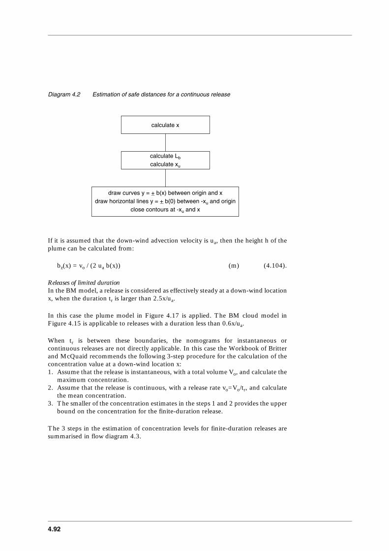
4.92
Diagram 4.2 Estimation of safe distances for a continuous release
If it is assumed that the down-wind advection velocity is u
a
, then the height h of theplume can be calculated from:
b
z(x) = vo / (2 ua b(x)) (m) (4.104).
Releases of limited durationIn the BM model, a release is considered as effectively steady at a down-wind locationx, when the duration tr is larger than 2.5x/ua.
In this case the plume model in Figure 4.17 is applied. The BM cloud model inFigure 4.15 is applicable to releases with a duration less than 0.6x/ua.
When tr is between these boundaries, the nomograms for instantaneous orcontinuous releases are not directly applicable. In this case the Workbook of Britterand McQuaid recommends the following 3-step procedure for the calculation of theconcentration value at a down-wind location x:1. Assume that the release is instantaneous, with a total volume Vo, and calculate the
maximum concentration.2. Assume that the release is continuous, with a release rate vo=Vo/tr, and calculate
the mean concentration.3. The smaller of the concentration estimates in the steps 1 and 2 provides the upper
bound on the concentration for the finite-duration release.
The 3 steps in the estimation of concentration levels for finite-duration releases aresummarised in flow diagram 4.3.
calculate x
calculate Lb
draw curves y = + b(x) between origin and xdraw horizontal lines y = + b(0) between -xu and origin
close contours at -xu and x
calculate xu
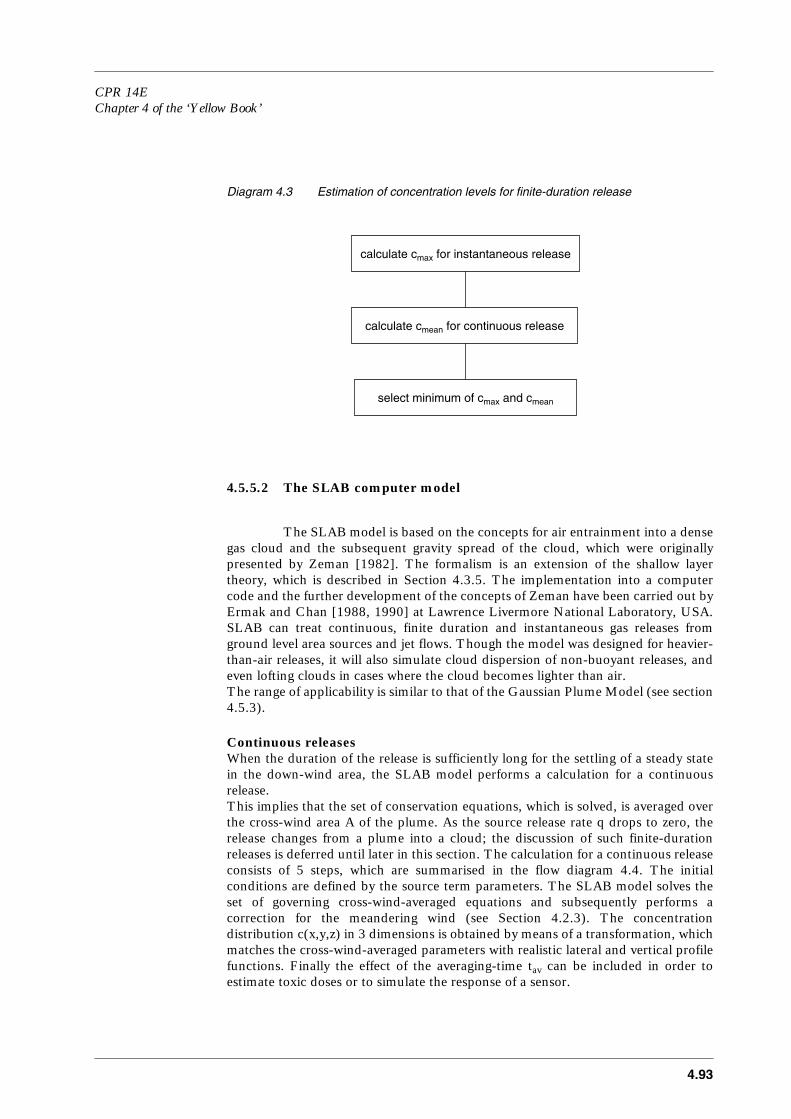
CPR 14EChapter 4 of the ‘Yellow Book’
4.93
Diagram 4.3 Estimation of concentration levels for finite-duration release
4.5.5.2 The SLAB computer model
The SLAB model is based on the concepts for air entrainment into a densegas cloud and the subsequent gravity spread of the cloud, which were originallypresented by Zeman [1982]. The formalism is an extension of the shallow layertheory, which is described in Section 4.3.5. The implementation into a computercode and the further development of the concepts of Zeman have been carried out byErmak and Chan [1988, 1990] at Lawrence Livermore National Laboratory, USA.SLAB can treat continuous, finite duration and instantaneous gas releases fromground level area sources and jet flows. Though the model was designed for heavier-than-air releases, it will also simulate cloud dispersion of non-buoyant releases, andeven lofting clouds in cases where the cloud becomes lighter than air.The range of applicability is similar to that of the Gaussian Plume Model (see section4.5.3).
Continuous releasesWhen the duration of the release is sufficiently long for the settling of a steady statein the down-wind area, the SLAB model performs a calculation for a continuousrelease.This implies that the set of conservation equations, which is solved, is averaged overthe cross-wind area A of the plume. As the source release rate q drops to zero, therelease changes from a plume into a cloud; the discussion of such finite-durationreleases is deferred until later in this section. The calculation for a continuous releaseconsists of 5 steps, which are summarised in the flow diagram 4.4. The initialconditions are defined by the source term parameters. The SLAB model solves theset of governing cross-wind-averaged equations and subsequently performs acorrection for the meandering wind (see Section 4.2.3). The concentrationdistribution c(x,y,z) in 3 dimensions is obtained by means of a transformation, whichmatches the cross-wind-averaged parameters with realistic lateral and vertical profilefunctions. Finally the effect of the averaging-time tav can be included in order toestimate toxic doses or to simulate the response of a sensor.
calculate cmax for instantaneous release
calculate cmean for continuous release
select minimum of cmax and cmean
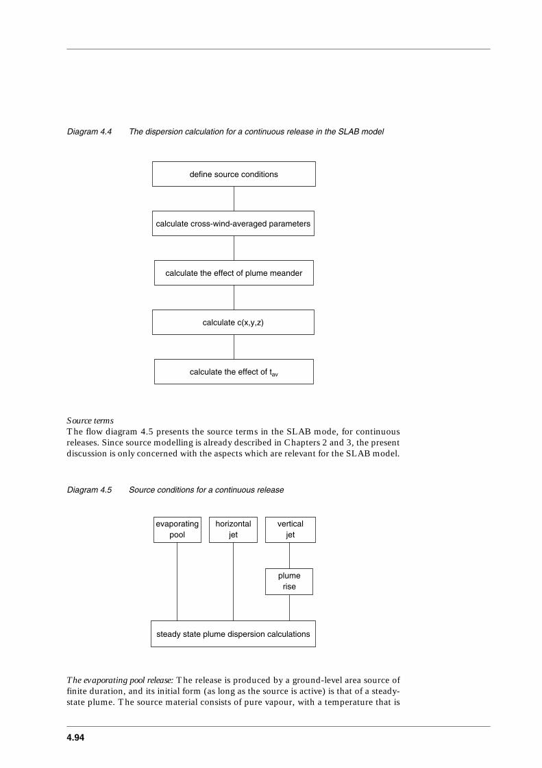
4.94
Diagram 4.4 The dispersion calculation for a continuous release in the SLAB model
Source termsThe flow diagram 4.5 presents the source terms in the SLAB mode, for continuousreleases. Since source modelling is already described in Chapters 2 and 3, the presentdiscussion is only concerned with the aspects which are relevant for the SLAB model.
Diagram 4.5 Source conditions for a continuous release
The evaporating pool release: The release is produced by a ground-level area source offinite duration, and its initial form (as long as the source is active) is that of a steady-state plume. The source material consists of pure vapour, with a temperature that is
define source conditions
calculate cross-wind-averaged parameters
calculate the effect of plume meander
calculate c(x,y,z)
calculate the effect of tav
evaporatingpool
plumerise
steady state plume dispersion calculations
horizontaljet
verticaljet

CPR 14EChapter 4 of the ‘Yellow Book’
4.95
equal to the boiling point of the chemical compound. In cases where the source areaA is not known, it is calculated from the evaporation rate uo using the equation
A = q / (ρo uo) (m2) (4.105).
q is the input mass source rate and ρo is the vapour density at the boiling pointtemperature of the chemical compound.The horizontal jet: The source is an area perpendicular to the ambient wind direction,and its outflow direction is pointing down-wind. The source material consists of asingle chemical compound, which may be partially liquid and partially vapour. Thevapour fraction is input. The jet temperature is also input, but this may not be belowthe boiling point of the chemical compared. The height of the source is an inputparameter.The vertical jet: The source is an area source and the source velocity is vertical, inupward direction. The source material consists of a single chemical compound, whichmay be partially liquid and partially vapour, similar to the horizontal jet. The heightof the source is an input parameter. Since the SLAB dispersion model can not handlecross-wind releases, the initial rise and down-wind bending of the jet release issimulated with the 1-dimensional integral model of Hoot, Meroney and Peterka[Hoot, 1973]. The shallow layer dispersion algorithm is used to describe the sinkingof the bent-over lofted plume, the touch-down phase, the slumped plume phase andthe far field behaviour. The procedure in SLAB to couple the HMP model outputresults to the input requirements of the shallow layer plume dispersion algorithm ispresented below. Note that it is different, and more complex, than the procedurerecommended in Section 4.5.4.2, formula (4.95).The procedure consists of 3 steps:– The peak concentration cr at maximal plume rise is calculated with the HMP
model, and then the cross-wind-averaged concentration c(xr) is obtained from theequation (note here c is to be expressed in parts per unit volume):
c(xr) = (0.524 (1-cr) + cr) cr (-) (4.106)
In the derivation of this equation it is assumed that the concentration profile isGaussian, so that the cross-wind-averaged concentration is 0.524 times the peakvalue. The additional terms in the equation are needed to ensure that c ≤ 1 forlarge values of cr.
– The HMP model assumes that the velocity of the bent-over plume is equal to theambient wind velocity ua. A correction is applied in SLAB for high densityreleases, where the down-wind plume velocity can be considerably smaller than ua.It is:
u(xr) = 0.5ua (1 - m - 2Cf + ((1-m)2 + 4mCf)1/2) / (1-Cf) (m s-1) (4.107),
Cf is a friction coefficient, with a value of 0.02, and m is the mass concentration,defined as:
m = µs c(xr) / (µa + (µs - µa) c(xr)) (-) (4.108).
µs and µa are molecular weights of the chemical compound and ambient airrespectively. The conversion from volume concentration c (m3/m3) to mass

4.96
concentration in (kg/kg) is needed because the internal calculations in SLAB aredone in ‘m’.
– To complete the description of the plume at the point of maximum plume rise, theplume half-width b, the height and centre height h need to be determined. Firstthe area of the plume cross-section at maximum plume rise is obtained from theequation
Ar = q / (ρ u m) (m2) (4.109).
q is the mass flow rate of the source. It is assumed that the half-height is 60% ofthe half-width:
by = 1.2 b (m) (4.110).
The plume centre height at maximal plume rise is h(xr) = hs + ∆hr.
The procedure is summarised in the Flow diagram 4.6.
In the region of plume rise, the trajectory (x,zc) of the plume centre is described bythe equation of an ellipse:
(1 - x/xr)2 + (h/∆hr - hs/∆hr)
2 = 1 (-) (4.112).
Diagram 4.6 Coupling of the HMP-model and the SLAB-model
For dispersion calculations of non-buoyant or positively buoyant releases it ispreferred to use the simple Gaussian plume model (Section 4.5.3), possibly incombination with Briggs plume rise formulae (Section 4.5.4), instead of thealgorithms in the SLAB model.
by max Ar / 2.4 ( ) , b o ( ) = (4.111).(m)
calculate c(xr)
apply correction for u(xr)
calculate b, bz and h(xr)
CPR 14EChapter 4 of the ‘Yellow Book’
4.97
The equations for a continuous release
The cross-wind-averaged plume properties are calculated in the SLAB model bynumerical integration of the governing equations.The set of equations consists of:
–
Cross-wind-averaged conservation equations of the total mass, the mass of thereleased chemical compound material, the momentum vector and the energy.
–
Equations for the width and height of the plume.
–
The equation of state, and other thermodynamic equations.The equations are solved by an integration in discrete steps in the down-windcoordinate. Since the temperature, the density and the vapour/liquid fraction in theplume are highly coupled quantities, the conservation equation of energy and thethermodynamic equations are solved together. This is done using Newton’s iterationmethod for each step of the integration in space. The other conservation equationsand the equations for the plume dimensions are ordinary differential equations. Theycan be solved by numerical integration using the Runge-Kutta method. Theevaluation of averaged quantities such as the average wind speed acting on the plumecan be done with Simpson’s rule.
The cross-wind-averaged conservation equations
For a plume the conservation equations of chemical compound material, total massand energy are:
d (m
ρ
uA) / dx = 0 (kg m
-1
s
-1
) (4.113),
d (
ρ
u A) / dx = 2
ρ
a
(b
y
w
e,t
+ b
z
w
e,e
) (kg m
-1
s
-1
) (4.114),
d (
ρ
u A c
p
T) / dx = 2
ρ
a
(b
y
w
e,t
+ b
z
w
e,e
) c
p,a
T
a
+ E
pc
+ E
gh
(J m
-1
s
-1
) (4.115).
The conservation equations of momentum are the equation for the down-wind plumevelocity u:
d (
ρ
u
2
A) / dx = -
ρ
a
d(g' Ab
z
) / dx + 2
ρ
a
u
a
(b
y
w
e,t
+ b
z
w
e,e
) + f
x
(N m
-1
) (4.116),and the equation for lateral gravity slumping u
y
:
For a lofted plume, the descent of plume height h is described with the momentumequation
The equation for gravity slumping in the y-direction is not needed in the lofted plumecalculation; then u
y
= 0. A lofted plume becomes grounded when h
≤
b
z
/2.The symbols for physical quantities and expressions used in 4.114-4.119 aresummarised in Table 4.11, which also includes the reference to the formulae wherethe expressions are evaluated.
d ρu u y A ( ) / dx 2 g ' ρ a b z 2 f y += (4.117),(N m
-1 )
d ρu u z A ( ) / dx – g ' ρ a A f z += (4.118),(N m -1 )

4.98
Table 4.11 Symbols in the conservation equations
Note that for the range of x-values that covers the source area, an additional term, thesource flux, must be included on the right-hand side of the mass and energyequations. For a surface source, when the chemical compound is released with avertical velocity u
o
, the surface flux term in the mass equations is given by 2
ρ
o
u
o
b
o
.
Ifthe temperature and the specific heat of the chemical compound at the source aredenoted by, respectively, T
o
and c
p,o
, then the surface flux term in the energyequation is given by 2
ρ
o
u
o
b
o
c
p,o
T
o
.
Ambient wind velocity profile
The entrainment velocities and the flux terms (friction terms, ground heat flux) arefunctions of the ambient wind. In the SLAB model the ambient wind velocity profileis derived from the gradient:
du
a
/dz = (u
*
/ (
κ
z)) f
m
(z/L) f
i
(z/h
i
) (s
-1
) (4.119),
u
a
is the ambient wind velocity, u
*
is the ambient friction velocity,
κ
= 0.41 is VonKarman’s constant, z is the height, L is the Monin-Obukhov length, h
i
is the heightof the mixing layer, f
m
is the momentum Monin-Obukhov function and f
i
(z/h
i
) is amixing layer function. The mixing layer function in SLAB is
Equation
x, y, z Spatial coordinates in down-wind direction and the horizontal and vertical cross-wind directions.
ρ
,
ρ
a
The densities in the plume and in ambient air. 4.138
T, T
a
The temperatures in the plume and in ambient air. 4.115, 4.136, 4.144b
m The mass concentration of the chemical compound. 4.113
u The down-wind plume velocity. 4.116
u
y
, u
x
1)
1)
u
x
appears in the instantaneous release model (4.163).
The velocities of plume spreading in the cross-wind directions.
4.117
u
z
Vertical velocity of the lofted plume 4.118
b
y
, b
z
, A The half-width, height and area (= 2b
y
b
z
) of the plume. 4.114, 4.117, 4.152
c
p
, c
p,a
The specific heats of the gas in the plume and of ambient air.
w
e,e
, w
e,t
The entrainment velocities at the edges and at the upper surface of the plume.
4.124-4.131
E
pc
The phase change energy per unit plume length. 4.144b
E
gh
The ground heat flux per unit plume length. 4.136-4.137
f
x
, f
y
, f
z
The friction terms in the 3 spatial directions. 4.132-4.135
g' The effective gravity g' = g
(ρ
o
-
ρ
a
)/ρa.
CPR 14EChapter 4 of the ‘Yellow Book’
4.99
fi(z/hi) = 1 - z / hi (-) (4.120a).
The substitution of the expressions for fm and fi, followed by an integration ofequation 4.119, yields
ua = (u* / κ) [ln(z/zo) + f(z/zo, z/L, z/hi)] (m s-1) (4.121).
f is a complicated function of its parameters. Section 4.5.2.1 provides a detaileddescription of the variation of ua with height. The computerised SLAB code uses asomewhat different but more complex function, which leads to only small differencesin ua above 100 m height. Near the ground, equation 4.119 gives meaningless results,so for small heights (z < 2.72 zo) ua is approximated by a polynomial:
ua = C1 z + C2 z2 (m s-1) (4.122).
The constants C1 and C2 are obtained by requiring that ua and dua/dz are continuousat the transition point z = 2.72.zo.
The average ambient wind velocity experienced by the dense gas cloud is
The integral can be calculated with Simpson’s rule.
Entrainment ratesWhile the entrainment concept is essential for the SLAB model, the choice of aparticular entrainment (sub)model is not an essential aspect of the model. Differentsubmodels could be used without changing the whole model. In the past years, theentrainment algorithms in SLAB have undergone several improvements. The versionwhich is discussed here [Ermak, 1990], distinguishes between vertical entrainment atthe top, and cross-wind and down-wind entrainment at the sides of the cloud (orplume).The vertical entrainment rate is defined to be
(u*)ic is the in-cloud value of the friction velocity, fi is the mixing layer function(4.120a) and fh is a Monin-Obukhov profile function. It is defined likewise as fm as
fm z/L( ) 1 5 z
L---+= (L ≥ 0)
fm z/L( ) 1/ 1 16z
L---–
1/2
= (L < 0) (-) (4.120b)
<ua> 1/bz ua z( ) dz
o
b
z
∫ = (4.123).(m s -1 )
we t, 1.5 3 κ u * ( ) ic f i b z / h i ( ) / f h b z /L ( ) = (4.124),(m s -1 )

4.100
f
h
(b
z
/L) = 1 + 5 b
z
/L (L
≥
0)
f
h
(b
z
/L) = 1/(1 - 16 b
z
/L)
1/2
(L < 0) (-) (4.125)
The friction velocity (u
*
)
ic
is calculated from a complicated mathematical expression,which is summarised in Diagram 4.7
Diagram 4.7 Calculation of the incloud friction velocity (u
*
)
ic
The horizontal cross-wind and down-wind entrainment rates are in the form(for continuous plumes only cross-wind entrainment is needed)
The term w
e,e,s
is a shear term. For cross-wind entrainment it is due to shear betweenthe cloud and the ambient atmosphere, and given by
w
e,e,s
= 0.209
κ
∆
u (m s
-1
) (4.127).
calculate
calculate
calculate
calculate
calculate
∆uρa
ρ-----<ua> u–( )=
u*( )mg2 u*/<ua>( )2 u 2 u y 2 /4+ ( ) 1/2+ u o u a =
u
*
( )
mh
2
0.0195
∆
u
2
ρ
a
ρ
-----u
y
2
+
/4=
u
*
( )
t
3
0.28 g u
*
< u a
> ------------ b z u * ( ) mg
T
a T
–
T
a
T
+
---------------- =
u
*
( )
ic
2
u
*
( )
mg
2
u
*
( )
mh
2
u
*
( )
t
2
+ +=
we,e 3 we,e,s2 we,e,t
2+( )( )1 2⁄
= (4.126).(m s-1)
CPR 14EChapter 4 of the ‘Yellow Book’
4.101
Here
∆
u is the velocity difference between plume and ambient air as defined inDiagram 4.7.
For down-wind entrainment the shear term is due to the increase in ambient velocitywith height. It is calculated from a complicated mathematical expression
The functions f
m
and f
i
have been defined in the discussion on the ambient windprofile (4.120a and 4.120b).The term w
e,e,t
describes the entrainment due to atmospheric turbulence and isidentical for the cross-wind and down-wind direction. It is given by
w
e,e,t
= 0.08 u (f
s
(L) f
p
(t
av
))
2
/ (f
s
(L) f
p
(t
av
) + 0.00144 b) (m s
-1
) (4.129).
t
av
is the averaging-time and b is either equal to b
x
(down-wind case for time-dependent cloud) or b
y
(cross-wind case). The functions are
Here, C
3
= 34.1 m.
The minimum averaging-time t
min
is 10 seconds. The normalisation time t
i
is takento be 900 seconds, which is the averaging-time that is assumed to apply to thestandard dispersion curves for passive gas.
In the limiting case of a passive gas release where all dense gas effects are negligible,SLAB yields a cloud concentration and size that correspond to the values fromstandard dispersion calculations.
Momentum flux terms
The velocity flux terms (or drag terms) that appear in the momentum equations ofthe SLAB model are adapted from the work of Zeman [1982]. They are needed inorder to determine the velocities and gravity currents u, u
x
(in an instanteous cloudonly), u
y
and u
z
in the dispersing release. The horizontal velocity fluxes f
x
and f
y
areboth composed of a term due to friction with the ground and a drag term at the topof the release. They are calculated from the equations:
f
x
= -2
ρ
b
y
((u
*
/<u
a
>)
2
[(u - ∆u)2 - <ua>2]+ 0.0195 ∆u2) (N m-1) (4.132)
we,e,s 0.6u*
κ----- f m
h
0.5
σ
z +
L
a
--------------------- f i
h
0.5
σ
z +
h
i
--------------------- = (4.128).(m s -1 )
fs L( )=1C3
L------
u*
<ua>------------– L < 0
fs L( )=1/ 1C3
L------
u*
<ua>-----------+
(4.130)(-)L > 0
fp tav( ) tav tminexp tav/tmin–( )+( )/ti( )0.2= (4.131).(-)
4.102
f
y
= -0.5
ρ
b
y
u
y2
[(u
*
/<u
a
>)
2
+ 0.0195 (
ρ
a
/
ρ
)
2
] (N m
-1
) (4.133).
The use of the equations is slightly different for plumes and clouds. For a plume, thevelocity flux term f
x
applies to down-wind movement of the dense gas in the plume,and the f
y
term determines the horizontal cross-wind gravity spreading. For a cloud,the f
x
term determines the average down-wind velocity u of the cloud as a whole, andthe f
y
term determines the gravity spreading with respect to the moving cloud centre,
both in down-wind and cross-wind direction. The term f z
due to vertical movementis not relevant for grounded releases, because the vertical velocity can be calculateddirectly from other quantities, without solving the vertical momentum equation.The SLAB model can also be applied to lofted plumes and clouds, but then there isno gravity spreading in the horizontal plane, so u
x
(in an instantaneous cloud) and u
y
are equal to zero. The movement of the cloud centre is affected only by drag due toshear with the surrounding air, so equation 4.130 applies without the ground frictionterm:
f
x
= -0.039
ρ
(2b
y
+ b
z
) (u
*
/<u
a
>)2 ∆u2 (N m-1) (4.134).
The vertical movement uz of the lofted plume or cloud is calculated by solving themomentum equation, with a drag term given by
fz = 0.039 ρ bz uz2 (N m-1) (4.135).
As explained before, fy is not needed for lofted plumes.
Heat flux termThe heat flux term is also obtained from the work of Zeman [1982]. The heat transferbetween the dense gas and the ground is represented in the energy equation by a term
Egh = 2 ρ by wH cp · (Ta - T) (J m-1 s-1) (4.136).
The effective heat transfer velocity wH is an empirical velocity, which also appears inother quantities such as the in-cloud friction velocity (u*)ic. It is given by
(u*)mg is defined in Diagram 4.7. For a lofted cloud Egh is, of course, equal to zero.
The thermodynamic modelThe SLAB computer model contains a submodel for the thermodynamic processeswhich occur during the dispersion of a mixture of liquids and vapours in theatmosphere. The submodel is restricted in the sense that it allows only phase changesof the released chemical compound and of ambient water vapour that enters therelease. The inclusion of moist air effects into the SLAB model requires thatadditional mass conservation equations are added for dry air and water. The equationof state for the complete system is
ρ = ρa Ta / (αl T + γl Ta) (kg m-3) (4.138),
wH = u
*
< u
a
>
------------ u * ( ) mg (4.137)(m s -1 )

CPR 14EChapter 4 of the ‘Yellow Book’
4.103
The coefficients
α
l
and
γ
l
are determined by the equations
α
l
=
µ
moist
(m
a
/
µ
a
+ m
w,v
/
µ
w
+ m
s,v
/
µ
s
) (-) (4.139),
µ
moist
= 1 / ((1 - m
w,va
)/
µ
a
+ m
w,va
/
µ
w
) (kg mol
-1
) (4.140),
γ
l
= (
ρ
a
/
ρ
w,l
)m
w,l
+ (
ρ
a
/
ρ
s,l
)m
s,l
(-) (4.141).
m is the mass concentration and
µ
is the molecular weight. The quantities are labeledwith 2 subscripts. The first subscript is either ‘a’, ‘w’ or ‘s’, and indicates whether thematerial is dry air, water or the chemical compound. The second subscript, separatedby the first subscript with a comma, is ‘v’ or ‘l’ and indicates the phase of the material,i.e. whether it is a vapour or a liquid. A superscript labels the material of theenvironment. Example: m
w,va
is the mass concentration of water vapour in ambientair. The vapour concentration is calculated separately for the chemical compoundand for water by using the condition of local equilibrium. This means that the partialpressure of the vapour phase of each material is equal to the smaller of 2 pressures:(1) the saturation pressure, or (2) the partial pressure when the total mass fraction isin the vapour phase.
For a single material the partial pressure after complete vaporisation (m
1
= 0) is
R is the gas constant. The saturation pressure is expressed in the form
p
a
is ambient pressure. C
A
, C
B
and C
C
are saturation pressure constants, which arebasic properties of the material. The constants C
B
and C
C
are required as inputparameters of the SLAB computer model. Then C
A
is calculated from 4.144 and the
boiling temperature (input to SLAB).
If the total mass concentration is denoted by m, then the local equilibrium conditionexpresses the vapour concentration as
m
v
= m (p < p
s
)
m
v
= m
⋅
(p > p
s
) (-) (4.144).
The procedure to evaluate the equation of state is summarised in Diagram 4.8.
Through the dependence of p
s
on the cloud temperature T, there is a strong couplingbetween the energy balance equation (4.115) and the thermodynamic state equations(4.138 - 4.144). The linking term is the phase change energy E
pc
, which depends onthe change of liquid material in the plume per down-wind distance (for thecontinuous release) or time (for the instantaneous release) integration step. For thecontinuous release E
pc
is described by:
p m
µ---- ρ RT / 1
ρ
ρ
a
----- γ l – = (4.142).(N m -2 )
ps pa exp C A C
B
T C
C
+
----------------- – = (4.143),(N m -2 )
ps
p----
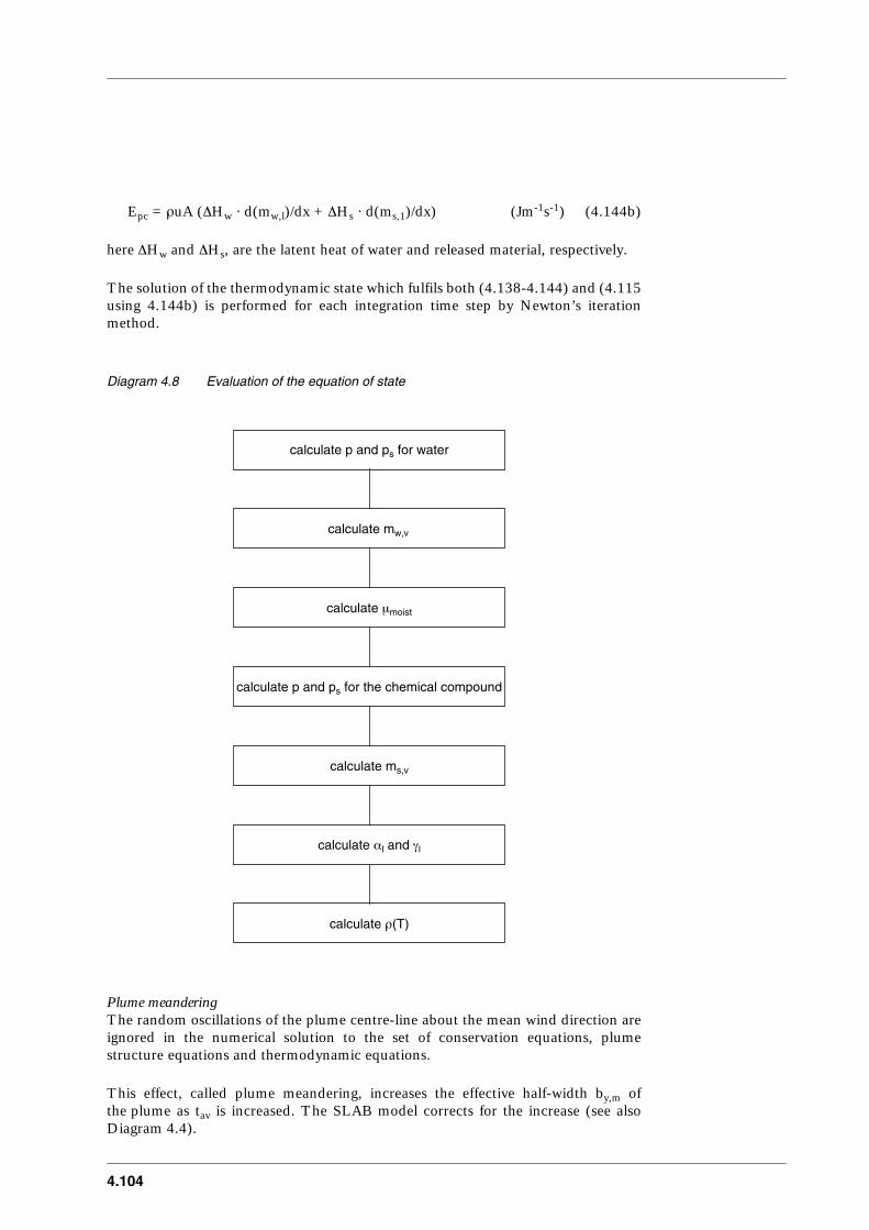
4.104
E
pc
=
ρ
uA (
∆
H
w
· d(m
w,l
)/dx +
∆
H
s
· d(m
s,1
)/dx) (Jm
-1
s
-1
) (4.144b)
here
∆
H
w
and
∆
H
s
, are the latent heat of water and released material, respectively.
The solution of the thermodynamic state which fulfils both (4.138-4.144) and (4.115using 4.144b) is performed for each integration time step by Newton’s iterationmethod.
Diagram 4.8 Evaluation of the equation of state
Plume meandering
The random oscillations of the plume centre-line about the mean wind direction areignored in the numerical solution to the set of conservation equations, plumestructure equations and thermodynamic equations.
This effect, called plume meandering, increases the effective half-width b
y,m
ofthe plume as t
av
is increased. The SLAB model corrects for the increase (see alsoDiagram 4.4).
calculate p and p
s
for water
calculate m
w,v
calculate p and p
s
for the chemical compound
calculate m
s,v
calculate
µ
moist
calculate
α
l
and
γ
l
calculate
ρ
(T)

CPR 14EChapter 4 of the ‘Yellow Book’
4.105
b
y,m2
= b
y2
+ 3 (r
2
(C
av
) - 1)
σ
y2
(t
av
) (m
2
) (4.145).
σ
y
is the standard deviation for a passive gas plume in the absence of plumemeandering. The averaging parameter C
av
is defined as
C
av
= (t
av
+ t
min
exp(-t
av
/t
min
) / t
min
)
0.2
(-) (4.146).
The exponential function exp is needed in order to guarantee that the averagingparameter becomes unity as t
av
approaches zero, because in this limit b
y,m
and b
y
should become equal. The exponent k is set equal to 0.2, in accordance with commonconventions. The effective minimum averaging-time t
min
is set equal to 10 seconds,since this has proven to give good results [Ermak, 1990].
The spatial concentration distribution in 3 dimensions
The SLAB plume model calculates only cross-wind-averaged properties, andcharacterises the shape by the height b
z
and the cross-wind half-width b
y
. Theparameters b
y
and b
z
do not correspond to a particular concentration level, butdescribe a surface which encloses the bulk of the dense gas. This means that the usercan implement a submodel of the concentration distributions which best fits hispurpose. In an early study of steady-state releases, Ermak et al. [1982] have used aquadratic distribution, but exponential or Gaussian distributions are otherpossibilities. The SLAB version, which is discussed here, assumes that thedistribution is Gaussian in the horizontal and vertical cross-sections:
c(x,y,z) = 2 b
y
b
z
c(x) F
y
(y,y
b
,C
y
) F
z
(z,h,
σ
z
) (parts per unit volume) (4.147),
The average volume concentration c(x) is related to the mass concentration by
c(x) = µa m(x) / (µs + (µa - µs) m(x)) (parts per unit volume) (4.148),
µs and µa are respectively the molecular weights of the chemical compound andambient air. The function Fy(y,yb,Cy) is defined as
erf denotes the error function, and yb and Cy are shape parameters. The shapeparameters are related: . yb follows from (4.153) below. Thefunction Fz(z,h,σz) is defined as
Fy y,yb,Cy( ) erf y yb+( )/ 2Cy( )( ) erf y yb–( )/( 2Cy( ) )–( )/ 4 y b ( ) =
(4.149),(m
-1
)
Cy2 1
3--by
2 yb2–( )=
Fz z,h,σz( ) exp z h–( )2/ 2σz2( )–( ) exp z h+( )2/ 2σz
2( )–( )+( )/ 2πσz2( )=
(4.150).(m-1)
4.106
h is the height parameter and σz is the vertical half-width parameter. The verticalprofile function allows for both grounded releases (h ≤ 0.5bz) and elevated releases(h > 0.5bz), with a width defined as
A number of additional cloud structure equations are needed in order to obtain acomplete description of the concentration distribution. They are, for a dispersingplume,
u dby/dx = (ρa/ρ) we,e + uy (m s-1) (4.152),
udyb/dx = uy yb/by (m s-1) (4.153),
u dh/dx = -uyh/by (m s-1) (4.154).
The initial conditions of by and h follow from the source dimensions bo and hs or theplume rise functions ((4.84) and (4.111)). The initial condition for yb is 0.9 times theinitial condition of by (to avoid Cy to become zero).
The equations can be solved with the Runge-Kutta method.
The effect of time-averagingThe last step in the Flow diagram 4.4 is to take a time-average at locations (x,y,z) overa duration of time tav. The averaging-time tav is an input parameter, in order to allowthe performance of calculations of the average concentration level for different timesof exposure. The time-averaged volume concentration cav is determined by averagingthe volume concentration c(x,y,z,t) over time:
The integration boundaries are tpk ± 0.5tav, where tpk is the time of peakconcentration. For a steady-state calculation, time-averaging has no effect.
This completes the description of the SLAB model in steady-state mode.
Finite-duration sources with a constant emission rateThe released gas of a finite-duration source is eventually advected down-wind as acloud instead of a plume, and this imposes different requirements on the dispersionalgorithms. The most important difference is that the governing equations arespatially averaged over the cloud volume instead of cross-wind-averaged. For a finite-duration release, SLAB starts in the plume submodel, and makes a transition to thepuff submodel at the time tr when the release is terminated. Thus, the calculation isperformed in 2 steps:
σz bz h–( )/ 3= (grounded)
σz 0.5 b z / 3= (lofted) (4.151).(m)
cmean x,y,z( ) 1/tav c x,y,z,t( ) dt ∫ = (4.155).(parts per unit volume)

CPR 14EChapter 4 of the ‘Yellow Book’
4.107
1. A calculation with the plume model is done, and the location x
c
(t) of thecorresponding cloud centre-of-mass at a time t is obtained by travelling down-wind until a location x
c
is reached where the plume contains half of the totalamount of dense gas, released during this time t. The cloud half-length is obtainedby a linear interpolation:
b
x
(t) = b
x
(0) + (b
x
(t
r
)-b
x
(0)) (x
c
(t)-x
c
(0)) / (x
c
(t
r
)-x
c
(0)) (m) (4.156).
x
c
(0) and b
x
(0) are the initial location of the centre-of-mass and the initial cloudhalf-length, which are determined by the source geometry. The half-width b
x
(t
r
)at the point of transition is calculated in step 2.
2. At the time t
r
the volume-averaged (puff) cloud properties are calculated from thecross-wind-averaged plume properties at the location x
c
(t
r
). It is assumed that themass fraction and the density are continuous at the transition, and then the cloudhalf-length is
b
x
(t
r
) = 0.5 u(x
c
) t
r
(m) (4.157),
where u(x
c
) is the down-wind cloud velocity at location x
c
.The cloud properties (u, T, b
y
, b
z,
etc.) are required to be equal to the plumeproperties at x = x
c
.The procedure is summarised in Flow diagram 4.9. The transformation is needed tostart the cloud calculation at t = t
r
, and it can also be applied to obtain cloudparameters for t < t
r
.
Diagram 4.9 Transformation of plume parameters to cloud parameters
Instantaneous releases
The SLAB model treats sources which inject a dense gas into the atmoshere at asteady rate, but during a finite time, as a cloud. The limiting case is an instantaneousrelease, for instance due to a tank failure. The calculation is performed with the puff
determine x
c
determine u(x
c
)
calculate b
x
equate m,
ρ
, u, T, b
y
, b
z
, ... at x = x
c

4.108
submodel, using a procedure consisting of 5 steps (see Flow diagram 4.10). The stepsdiffer from the procedure of the plume submodel (see Flow diagram 4.4) in a numberof aspects, which are discussed in the remainder of this Section.
Diagram 4.10 The dispersion calculation for an instantaneous release in the SLAB model
The instantaneous or short-duration evaporating pool:
Although the source is of theground-level area type, it differs from the previous types in that the release occursinstantaneously or in a very short time. The amount of released chemical compoundis not characterised by the mass rate q, but by the total mass Q. This type of releaseis usually accompanied by compressibility effects (see chapter 2), but the source termmodel in SLAB assumes that the cloud is fully expanded and that the pressure hasbeen reduced to the ambient atmospheric level. The source material consists of purevapour.
The equations for an instantaneous release
The conservation equations, the cloud structure equations and the thermodynamicequations are solved by an integration in discrete steps in the time coordinate. Thenumerical techniques which were indicated in the discussion of the plume model, areequally applicable to the puff model.
The volume-averaged conservation equations
For a cloud the conservation equations of species, mass and energy are:
d (m
ρ
V) / dt = 0 (kg s
-1
) (4.158),
define source conditions
calculate average parameters for the cloud volume
calculate the effect of cloud meander
calculate c(x,y,z,t)
calculate the effect of tav
CPR 14EChapter 4 of the ‘Yellow Book’
4.109
d (
ρ
V) / dt =
ρ
a
v
e
(kg s
-1
) (4.159),
d (
ρ
V c
p
T) / dt =
ρ
a
v
e
c
pa
T
a
+ 2 b
x
(E
pc
+ E
gh
) (J s
-1
) (4.160),
v
e
= 4 (b
y
b
z
w
e,x
+b
x
b
z
we,y + bx by we,t) (m3 s-1) (4.161).
The down-wind entrainment velocity we,x and the cross-wind entrainment velocitywe,y are obtained from equation 4.126. The vertical entainment velocity we,t isobtained from equation 4.124.
The momentum equation for the centre-of-mass of the cloud is
d (ρ u V) / dt = ρa ve ua + 2 bx fx (N) (4.162).
The gravity slumping equations for a grounded cloud are
For a lofted cloud, the equations 4.163-4.164 are replaced by the momentumequation of vertical momentum:
The spatial concentration distribution in 3 dimensionsThe characterisation of the cloud shape requires a third parameter, the down-windhalf-length bx, in addition to by and bz.They are obtained by solving the cloud structure equations:
dby/dt = (ρa/ρ) we,y + uy (m/s) (4.166),
dyb/dt = uy yb / by (m/s) (4.167).
Since a cloud has a finite extension at each location x in the down-wind direction, theterm c(x) in the 3-dimensional concentration distribution c(x,y,z,t) contains a down-wind profile function. It is defined as
c(x) = 2 bx c(t) Fx(x-xc,xb,Cx) (parts per unit volume) (4.168),
where the average volume concentration c(t) is related to m(t) through equation4.148, and the profile function Fx is equal to Fy as defined in equation 4.149, theposition of the centre-of-mass of the cloud, xc is calculated by integrating u from(4.162) to time t. Cx follows from . The cloud structure equationsfor bx and xb are
dbx/dt = (ρa/ρ) we,x + ux (m s-1) (4.169),
d ρ u x V ( ) / dt g ' ρ a b x b z 2 2 b x f y += (4.163),(N)
d ρ u y V ( ) / dt g ' ρ a b y b z 2 2 b x f y += (4.164).(N)
d ρ u z V ( ) / dt g – ' ρ a V 2+ b x f z = (4.165).(N)
Cx2 1
3-- bx
2 xb2–( )=

4.110
dx
b
/dt = u
x
x
b
/ b
x
(m s
-1
) (4.170).
The equations can be solved with the Runga-Kutta method.The initial conditions for b
x
follow from the source dimensions or equation 4.157.The initial condition for x
b
is 0.9 times the initial condition of b
x
.
The effect of time-averaging
The calculation of the time-averaged volume concentration c
av
(x,y,z) requires theevaluation of the time-integral.An analytical expression can be derived:
t
pk
is the time of peak concentration. The terms F
y
and F
z
are spatial distributionfunctions, which were defined in the discussion of continuous releases.
This ends the discussion of instantaneous releases in the SLAB model.
cav x,y,z( ) 4 b x b y b z c t pk ( ) f av x b , C x , t av ( ) F y y , y b , C y ( ) F z z , h , σ z ( ) =
(4.171),(parts per unit volume)
fav xb,Cx,tav( )Cx
2 x b u t av -------------------------- x
1 erf x 1 ( ) x 2 erf x 2 ( ) –
1
π ------ e
x
12
–
e x
22
–
– +
=
(4.172),(m
-1
)
x1 xb1
2--u t av +
/ 2 C x ( ) = (4.173),(-)
x2 xb1
2--– u t av
/ 2 C x ( ) = (4.174).(-)

CPR 14EChapter 4 of the ‘Yellow Book’
4.111
4.6 Application of selected models: calculation examples
4.6.1 Introduction to Section 4.6
Section 4.6 provides examples on the use of models described inSection 4.5.Section 4.6.2 provides examples on stability calculations using the Holtslag schemeas presented in Section 4.5.2.Section 4.6.3 considers the use of the Gaussian plume model for continuous andinstantaneous releases as described in Section 4.5.3.Section 4.6.4 provides examples on the calculation of free jets, plume rise and theplume trajectory model (HMP-model) as described in Section 4.5.4.Section 4.6.5 provides examples on the use of the SLAB model as described inSection 4.5.5.
4.6.2 Examples of stability calculations
This section provides examples on the use of the Holtslag scheme, Section4.5.2. In Section 4.6.2.1 the application of the day-time scheme and in Section4.6.2.2 the application of the night-time scheme is presented.
4.6.2.1 Application of the day-time scheme
The site for which the stability is to be established is somewhere in TheNetherlands: 51˚ N, -5˚ W.The day is the 20
st
of June (in a non-leap year), the time 9.40 UTC locally beforenoon.The weather is overcast with broken clouds, N = 6/8, and the air temperature is about20 ˚C.The wind speed at 10 m height is 4 m/s. The terrain is flat, grass-covered, withoutobstacles; the roughness length z
o
is estimated to be 0.01 m, see Table 4.3.The albedo is estimated from Table 4.4 and found to be 0.2; the moisture availabilityis set at 1.From Appendix I, we calculate the Julian day to be 171, and the solar elevation 48.6˚;(the solar longitude SL = 7.87, the solar declination SD = 0.409, and
α
= -0.704). Byuse of formulae (4.36) to (4.38) the sensible heat flux is calculated to be 72.9 W/m
2
. Iteratively we calculate L and u
*
: L = -21.7 m and u
*
= 0.260 m/s by use of (4.35).Observing Golder’s graph (Figure 4.11) we find that the unstable situation is to beclassified as Pasquill C, so the mixing height is set at 1000 m.
For these calculations we have used c
p,a
= 1000 W/kg K,
ρ
a
at 293 K = 1.2 kg/m
3
and
γ
= 0.45 (Table 4.5).
The input, output and intermediate results are summarised in the following table:

4.112
Table 4.12 Day-time stability calculation
4.6.2.2 Application of the night-time scheme
For this example the same site as used in Section 4.6.2.1 is selected.The sky is clear (N = 0); the wind speed is now 4.5 m/s at 10 m height. Thetemperature is 20 ˚C (293 K) and the wet bulb temperature is 18 ˚C (291 K).By use of formulae (4.40) to (4.46) we iteratively find the sum of heat fluxesminimised by using a Monin-Obukhov length L = 17.3 m. The friction velocityu
*
= 0.184 m/s. For this situation we find the following heat fluxes:
This situation can be classified as Pasquill E, see Figure 4.11.For the mixing height we need to calculate the Coriolis parameter f for conditions inThe Netherlands: latitude 51˚. This leads to f = 1.13 . 10
-4
s
-1
. By use of Table 4.7the mixing height is calculated to be 291 m.Input and output are summarised in Table 4.13.
Input positiondaytimecloud cover Nwind speed U
a
(10)roughness length z
o
albedo emoisture availability
α
51˚ N -5˚ WJune 20st9.40 UTC6/84 m/s0.01 m0.21
Intermediate results solar radiation H
rs
Net radiation H
r
511.9 W/m
2
332.7 W/m
2
Output sensible heat flux H
o
Monin-Obukhov length Lfriction velocity u
*
Pasquill classmixing height h
i
72.9 W/m
2
-21.7 m0.260 m/sC1000 m
net radiation H
r
= -51.3 W/m
2
sensible heat flux H
o
= -23.2 W/m
2
ground heat flux H
g
= -25.3 W/m
2
latent heat flux H
l
= -2.8 W/m
2
balance: -51.3 -51.3 W/m
2
CPR 14EChapter 4 of the ‘Yellow Book’
4.113
Table 4.13 Night-time stability calculation
4.6.3 Application of the Gaussian plume model
In this section two examples are discussed. The concentration below anelevated plume and the LEL contour is calculated for a continuous release and thecalculation of the time series and explosive content for an instantaneous release offinite dimensions are shown.
4.6.3.1 Calculations of a plume
In this example the meteorological situation is described using Pasquillstability class, with a neutral atmosphere (class D) and the surroundings of the sitecan be described as “habitated land”.
Natural gas (methane) is released continuously at a release rate of 20 kg/s and wewant to know the 10-minute averaged concentration at 1.5m height below the plumecenterline and the contour defined by the LEL concentration.
Input cloud cover Nwind speed u
a
(10)roughness length z
o
T
a
(2 m)T
w
(2m)
04.5 m/s0,01 m293 K291 K
Intermediate results T
*
T
r
(50 m)T
o
(z
o
)T
s
H
ri
H
r
H
o
H
g
K
s
H
l
0.086 K294.4 K291.8 K289.3 K-80.7 W/m
2
-51.3 W/m
2
-23.2 W/m
2
-25.3 W/m
2
0.0236-2.8 W/m
2
Output sensible heat flux H
o
Monin-Obukhov length Lfriction velocity u
*
Pasquill classmixing height h
i
-23.2 W/m
2
43 m0.223 m/sE291 m
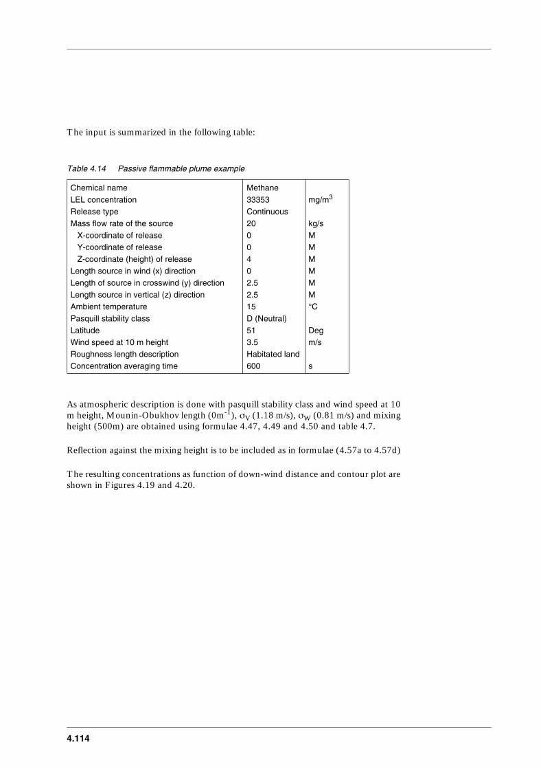
4.114
The input is summarized in the following table:
Table 4.14 Passive flammable plume example
As atmospheric description is done with pasquill stability class and wind speed at 10m height, Mounin-Obukhov length (0m
-1
),
σ
V
(1.18 m/s),
σ
W
(0.81 m/s) and mixingheight (500m) are obtained using formulae 4.47, 4.49 and 4.50 and table 4.7.
Reflection against the mixing height is to be included as in formulae (4.57a to 4.57d)
The resulting concentrations as function of down-wind distance and contour plot areshown in Figures 4.19 and 4.20.
Chemical name Methane LEL concentration 33353 mg/m
3
Release type Continuous Mass flow rate of the source 20 kg/s X-coordinate of release 0 M Y-coordinate of release 0 M Z-coordinate (height) of release 4 MLength source in wind (x) direction 0 MLength of source in crosswind (y) direction 2.5 MLength source in vertical (z) direction 2.5 MAmbient temperature 15 °CPasquill stability class D (Neutral) Latitude 51 DegWind speed at 10 m height 3.5 m/sRoughness length description Habitated land Concentration averaging time 600 s

CPR 14EChapter 4 of the ‘Yellow Book’
4.115
Figure 4.19 Concentration [mg/m
3 ] as function of down-wind distance [m] at
y = 0m and z = 1.5m
Figure 4.20 Concentration contour plot for LEL [33353 mg/m
3
] at 1.5m heightt
Down-wind distance [m]250240230220210200190180170160150140130120110100908070605040302010
Con
cent
ratio
n [m
g/m
3]66,000
64,000
62,000
60,000
58,000
56,000
54,000
52,000
50,000
48,000
46,000
44,000
42,000
40,000
38,000
36,000
34,000
32,000
30,000
28,000
26,000
24,000
22,000
20,000
18,000
16,000
14,000
12,000
10,000
8,000
6,000
4,000
2,000
0
Distance down-wind (x) [m]353025201510
Dis
tanc
e cr
oss-
win
d (y
) [m
]
4
3
2
1
0
-1
-2
-3
-4

4.116
4.6.3.2 Calculation of explosive mass of an instantaneous puff
For this example use is made of the same meteorological and site conditionsas for the previous one: pasquill class D, wind speed of 3.5m/s and habitated land.
The source is assumed to be a cube with sides of 21m, originating from e.g. an initiallyexpanding cloud. This initial cube contains 6000kg of natural gas (methane) atnormal ambient conditions (1 atm, 15˚C). For the calculation, the source parametersare represented by b0x = b0y = b0z =10.5m; h = 10.5m.
The input is summarized in Table 4.15
Table 4.15 Input for instantaneous release example
The resulting concentration as function of time at a position and explosive massevolution are shown in Figures 4.21 and 4.22.
The explosive contents are calculated with a numerical 3D integration of one of thehalves of the cloud, as this one is symmetric with respect of the xz plane at 0 crosswinddistance.
Chemical name MethaneRelease type InstantaneousTotal mass released 6000 KgLength source in wind (x) direction 21 MLength of source in crosswind (y) direction 21 MLength source in vertical (z) direction 21 MAmbient temperature 15 °CPasquill stability class D (Neutral)Latitude 51 DegWind speed at 10 m height 3.5 m/sRoughness length description Habitated land
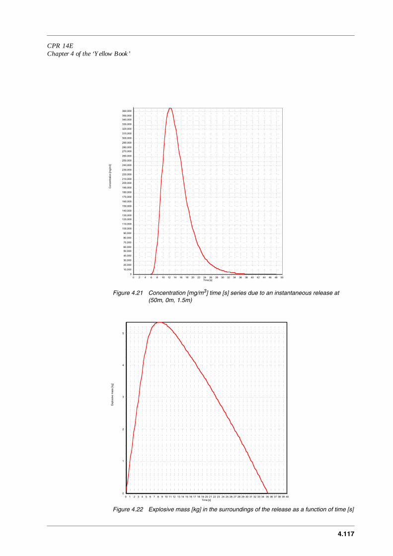
CPR 14EChapter 4 of the ‘Yellow Book’
4.117
Figure 4.21 Concentration [mg/m3] time [s] series due to an instantaneous release at (50m, 0m, 1.5m)
Figure 4.22 Explosive mass [kg] in the surroundings of the release as a function of time [s]
Time [s]50484644424038363432302826242220181614121086420
Con
cent
ratio
n [m
g/m
3]360,000
350,000
340,000
330,000
320,000
310,000
300,000
290,000
280,000
270,000
260,000
250,000
240,000
230,000
220,000
210,000
200,000
190,000
180,000
170,000
160,000
150,000
140,000
130,000
120,000
110,000
100,000
90,000
80,000
70,000
60,000
50,000
40,000
30,000
20,000
10,000
0
Time [s]403938373635343332313029282726252423222120191817161514131211109876543210
Exp
losi
ve m
ass
[kg]
5
4
3
2
1
0
4.118
There is a quick dilution of the cloud even in neutral atmospheric conditions due toa relative high wind speed and to the type of land (habitated), which increases theturbulence at ground level; the maximum explosive mass is 5.35kg just 8.35s after therelease.
4.6.4 The application of models for jets and plumes
4.6.4.1 The free jet model
The example calculation to illustrate the use of the free jet formalism is apositively buoyant jet in vertical, upward direction, in a homogeneous atmospherewith zero wind speed. A release of this type could occur due to:– A punctured vessel or a ruptured pipeline, at a small containment overpressure,
since the outflow is subsonic.– A sonic release from a punctured or ruptured container at a high pressure, when
the source parameters are derived in the region after the initial expansion toambient pressure. The procedures which allow to obtain subsonic sourceparameters from a sonic source configuration are discussed in chapter 2.
The input data for a typical case, a natural gas (NG) jet, are summarised inTable 4.17, although, it must be mentioned that the exit velocity is about one thirdof the speed of sound. The calculation consists of 3 steps:– Calculate the Froude number of the source to determine at what range of down-
stream distances the jet model can be applied, and where the release should betreated as a plume (4.71-4.72).
– Evaluate the axial concentration decay, and correct for density effects (4.76,4.78).
– Calculate isocontours and the NG contents in the flammable part (4.81, 4.82).The numbers in parentheses indicate the relevant equations. The results of thecalculations are presented in Figure 4.23. The NG flammable contents is 7.5 kg.
CPR 14EChapter 4 of the ‘Yellow Book’
4.119
Figure 4.23 Example of concentration contours (UFL and LFL) of a free jet, see Section 4.5.4.1
Table 4.16 Input data for the free jet model
4.6.4.2 The application Briggs plume rise formulae
The Briggs formulae are intended for plume rise predictions of the hotgases, which are emitted from tall stacks. In such cases the temperature differencebetween the pollutant and the surrounding air is large, and the dispersing plume hasa large buoyancy flux factor. Within the framework of the Yellow Book, a possibleapplication of the Briggs formulae is the dispersion of smoke plumes from fires. Theexample to illustrate the formalism is a vertical upward plume of hot air, which isreleased from a circular source in a neutral atmosphere.The input data of the example are summarised in Table 4.18. The calculationconsists of 3 steps:– Calculate the buoyancy flux factor and the distance to final plume rise (4.88-
4.91). Note that the plume rise is limited by (4.91).
source diameter [m]exit velocity [m/s]NG density [kg/m3]ambient density [kg/m3]UFL [%]LFL [%]
2 bo
uo
ρo
ρa
--
0.2150
0.781.21
155.3
LEL UEL
Axial Distance [m]1211109876543210
Rad
ial d
ista
nce
[m]
0.5
0
-0.5

4.120
– Calculate the contributions of initial momentum and buoyancy to the total plumerise (4.88, 4.92).
– Calculate the total plume rise by adding the third powers of the 2 contributions.In general the release of large sources is buoyancy-dominated due to thex2/3-dependency, as opposed to the x1/3-dependency of the momentum-contribution (4.93).
According to the Briggs formulae the down-wind distance to final plume rise is348 m. The contributions of initial momentum and buoyancy to the plume rise are,respectively, 30 m and 97 m. So the total plume rise is equal to 98 m.
Table 4.17 Input data for Briggs plume rise formulae
4.6.4.3 The integral model of Hoot, Meroney and Peterka
This section contains an example to illustrate the use of the 1-dimensionalintegral model of Hoot, Meroney and Peterka [HMP, 1973]. The release is anegatively buoyant jet in vertical, upward direction, and the environment is ahomogeneous atmosphere. The input data of the example, a release of chlorine atambient conditions, are summarised in Table 4.19.
Table 4.18 Input data for the HMP model
It can be calculated from the equations in Section 4.5.4 (4.83 and 4.84, using g =9.81 m/s2) that the plume rise is at its maximum (∆hr = 11.6 m) at a down-winddistance xr of 6.9 m. The peak concentration of chlorine at maximum plume rise is11.4% (formula 4.86).The plume starts to descend from the point of maximal plume rise, because the plumematerial is still heavier than air. The HMP model contains formulae to calculate thedown-wind distance of plume touch-down and the approximate concentration at thatpoint (roughly 7% at xg = 49 m), but the user of the Yellow Book is advised toperform the calculations of the plume sinking, touch-down and possiby slumpingwith the SLAB computer model (see the Section 4.5.5.2), or with the simple
source diameter [m]exit velocity [m/s]density of air (150 ˚C) [kg/m3]ambient density [kg/m3]wind velocity m/s]
2 bo
uo
ρo
ρa
ua
4100.841.204
source diameter [m]exit velocity [m/s]source height [m]chlorine density [kg/m3]ambient density [kg/m3]wind velocity m/s]
2 bo
uo
hs
ρo
ρa
ua
125203.001.214

CPR 14EChapter 4 of the ‘Yellow Book’
4.121
Gaussian plume model. The SLAB model contains the HMP model as a submodel,so the whole calculation, including initial plume rise, can be done with SLAB.
4.6.5 The application of dense gas dispersion models
The SLAB computer model can be applied to dense gas releases from long-duration pool evaporation, from horizontal and vertical two-phase jets, and fromshort-duration or instantaneous pool releases. The present section contains anexample calculation for each of these four source term submodels, in order toillustrate the use of the SLAB model. The examples of the long- and short-durationpool evaporation are also used to illustrate the use of Britter and McQuaid’snomograms.
4.6.5.1 Long-duration pool evaporation
The example to illustrate the pool evaporation source type is a liquid poolof chlorine, caused by a leaking storage drum. The source characteristics were alreadydiscussed as an example in Chapter 3. The release disperses as a plume over an area,which is overgrown with low crops. The input data for the SLAB computer model aresummarised in Table 4.20. The values for the chlorine source material have beenobtained from the table of material properties in the SLAB user manual [Ermak,1990]. The duration of 200 seconds is sufficient to obtain, for the present range ofdown-wind distances (1 km), a steady-state solution with the SLAB computer model.
4.122
Table 4.19 SLAB input for a long-duration evaporating pool of chlorine
An isocontour of the chlorine concentration of 15 g/m3, corresponding to a molarfraction of 0.5%, at a height of 1.5 m above ground-level (i.e. at inhalation level) att = 200 s after the start of the evaporation, has been calculated with SLAB, and theresults are shown in Figure 4.24.
Definition of source term: evaporating pool, long-duration
IDSPL = 1
Definition of numerical step: largest step size NCALC = 1Molecular weight of source material [kg]: 0.070906 (chlorine) WMS = 0.070906Vapor heat capacity of source material at constant pressure [J/kg K]:
498.1 (chlorine) CPS = 498.1
Boiling point temperature of source gas [K]: 239.1 (chlorine) TBP = 239.10Initial liquid mass fraction of source material: 1.0 (liquid) CMEDO = 1.0Heat of vaporisation of the source material at the boiling point temperature [J/kg]:
287840.0 (chlorine) DHE = 287840.
Liquid specific heat of the source material [J/kg K]: 962.35 (chlorine) CPSL = 962.35Liquid density of the source material [kg/m3]: 1574.0 (chlorine) RHOSL = 1574.0First saturation constant of source material [-]: 1978.34 (chlorine) SPB = 1978.34Second saturation constant of source material [K]: -27.01 (chlorine) SPC = -27.01Temperature of the source material [K]: 239.1 TS = 239.1Mass flow rate of the source [kg/s]: 5.0 QS = 5.0Area of the source [m2]: 100.0 AS = 100.0Duration of the release, for a finite-duration source [s]:
200. TSD = 200.
Source mass, for an instantaneous release [kg]: 0 QTIS = 0Height of the source [m]: 0. HS = 0Concentration averaging-time [s]: 60. TAV = 60Maximum down-wind distance in the calculation [m]:
1000. XFFM = 10000
First height where the concentration is calculated [m]:
1.5 ZP(1) = 1.5
Second height where the concentration is calculated (is used only when ZP(1) > 0) [m]:
0. ZP(2) = 0
Third height where the concentration is calculated (is used only when ZP(1:2) > 0) [m]:
0. ZP(3) = 0
Fourth height where the concentration is calculated (is used only when ZP(1:3) > 0) [m]:
0. ZP(4) = 0
Surface roughness height [m]: 0.1 (low crops) Z0 = 0.1Measurement height of ambient parameters [m]: 10. ZA = 10Ambient wind speed [m/s]: 5. UA = 5Temperature of ambient air [K]: 288.15 TA = 288.15Relative humidity of ambient air [%]: 70. RH = 70Stability class: 4 (Pasquill class D) STAB = 4
CPR 14EChapter 4 of the ‘Yellow Book’
4.123
Figure 4.24 Contour of a concentration of 15 g/m3 chlorine due to an evaporating pool
The chlorine concentration was also estimated with the model of Britter andMcQuaid. The nomogram for continuous releases should be read with the parameter((go
')2vo/ua5)1/5 = 0.697 along the horizontal axis, and along the
vertical axis (see Section 4.5.4.1, the density of chlorine at boiling point is3.61 kg/m3). The largest distance to c = 0.5% is about 210 m. The difference withSLAB might be due to heat transfer effects.
4.6.5.2 Horizontal jet
The example to illustrate the horizontal jet source type is a jet of propane,of pure vapour, emerging from a ruptured pipeline of a railway tank wagon. Thesource characteristics were already discussed as an example in Chapter 2. The releasedisperses as a plume over an area, which is overgrown with low crops. The input datafor the SLAB computer model are summarised in Table 4.21. The values for thepropane source material have been obtained from the table of material properties inthe SLAB user manual.
Distance down-wind (x) [m]5550454035302520151050
Dis
tanc
e cr
oss-
win
d (y
) [m
]
8
6
4
2
0
-2
-4
-6
-8
x/ vo/ua( ) 1.9 x=

4.124
Table 4.20 SLAB input for a horizontal propane jet
The isocontour of the propane concentration of 9.3 g/m3 (molar fraction 0.5%) at aheight of 1.5 m above ground-level at t = 1500 s after the start of the release, has beencalculated with SLAB, and the results are shown in Figure 4.25.
Definition of source term: horizontal jet IDSPL = 2
Definition of numerical step: largest step size NCALC = 1
Molecular weight of source material [kg/mol]: 0.044097 (propane) WMS = 0.044097
Vapor heat capacity of source material at constant pressure [J/kg K]:
1678. (propane) CPS = 1678.
Boiling point temperature of source gas [K]: 231.09 (propane) TBP = 231.09
Initial liquid mass fraction of source material: 0 (pure vapour) CMEDO = 0
Heat of vaporisation of the source material at the boiling point temperature [J/kg]:
425740. (propane) DHE = 425740.
Liquid specific heat of the source material[J/kg K]:
2520. (propane) CPSL = 2520.
Liquid density of the source material [kg/m3]: 500.5 (propane) RHOSL = 500.5
First saturation constant of source material [-]: 1872.46 (propane) SPB = 1872.46
Second saturation constant of source material [K]: -25.16 (propane) SPC = -25.16
Temperature of the source material [K]: 231.1 TS = 231.1
Mass flow rate of the source [kg/s]: 7.85 QS = 7.85
Area of the source [m2]: 3.14 AS = 3.14
Duration of the release, for a finite-duration source [s]:
1500 TSD = 1500
Source mass, for an instantaneous release [kg]: 0. QTIS = 0
Height of the source [m]: 3.0 HS = 3
Concentration averaging-time [s]: 0.1 TAV = 0.1
Maximum down-wind distance in the calculation [m]:
500. XFFM = 1000
First height where the concentration is calculated [m]:
0. ZP(1) = 0.
Second height where the concentration is calculated (is used only when ZP(1) > 0) [m]:
0. ZP(2) = 0
Third height where the concentration is calculated (is used only when ZP(1:2) > 0) [m]:
0. ZP(3) = 0
Fourth height where the concentration is calculated (is used only when ZP(1:3) > 0) [m]:
0. ZP(4) = 0
Surface roughness height [m]: 0.1 (low crops) Z0 = 0.1
Measurement height of ambient parameters [m]: 10. ZA = 10
Ambient wind speed [m/s]: 2. UA = 2
Temperature of ambient air [K]: 288.15 TA = 288.15
Relative humidity of ambient air [%]: 70. RH = 70
Stability class: 6 (Pasquill class F) STAB = 6
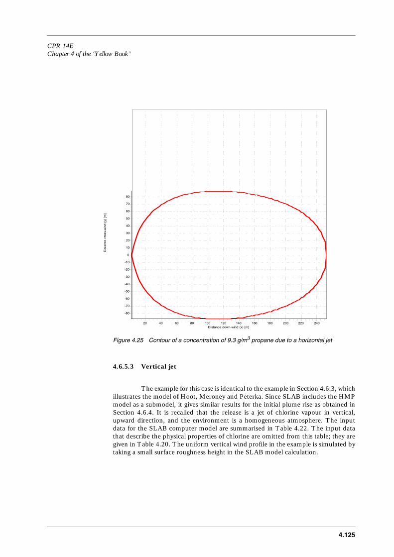
CPR 14EChapter 4 of the ‘Yellow Book’
4.125
Figure 4.25 Contour of a concentration of 9.3 g/m3 propane due to a horizontal jet
4.6.5.3 Vertical jet
The example for this case is identical to the example in Section 4.6.3, whichillustrates the model of Hoot, Meroney and Peterka. Since SLAB includes the HMPmodel as a submodel, it gives similar results for the initial plume rise as obtained inSection 4.6.4. It is recalled that the release is a jet of chlorine vapour in vertical,upward direction, and the environment is a homogeneous atmosphere. The inputdata for the SLAB computer model are summarised in Table 4.22. The input datathat describe the physical properties of chlorine are omitted from this table; they aregiven in Table 4.20. The uniform vertical wind profile in the example is simulated bytaking a small surface roughness height in the SLAB model calculation.
Distance down-wind (x) [m]24022020018016014012010080604020
Dis
tanc
e cr
oss-
win
d (y
) [m
]
80
70
60
50
40
30
20
10
0
-10
-20
-30
-40
-50
-60
-70
-80

4.126
Table 4.21 SLAB input for a vertical chlorine jet
The output results show that the region of maximal plume rise appears at down-winddistances between 6.1 and 7.6 m, with a final rise of 9.7 m and a cross-wind-averagedconcentration of 8.3%. It is noted that these results are slightly different from thecalculation in Section 4.6.3, because the surface roughness in SLAB introduces anon-constant vertical wind profile. In the SLAB model simulation, the plume touch-down occurs at a down-wind distance of 43 m, with a cross-wind-averagedconcentration of 4.6%. Upon touch-down of the plume, a transition occurs from anairborne plume with a diameter of 8 m to a slumped plume with a height of 2.8 monly. Pressure forces develop during the transition which are converted intohorizontal momentum, mainly in the cross-wind direction, resulting in a rapidbroadening of the slumped plume. Ultimately differences in velocity between theplume and ambient atmosphere become negligible, and the dispersion processresembles that of a steady plume. Figure 4.26 shows an isocontour of the chlorineconcentration (15 g/m3 corresponding to a molar fraction of 0.5%) at ground level,at t = 600 s after the start of the release calculated with SLAB.
Definition of source term: vertical jet IDSPL = 3Definition of numerical step: largest step size NCALC = 1Temperature of the source material [K]: 293.1 TS = 293.1Mass flow rate of the source [kg/s]: 58.9 QS = 58.9Area of the source [m2]: 0.785 AS = 0.785Duration of the release, for a finite-duration source [s]: 600. TSD = 600Source mass, for an instantaneous release [kg]: 0 QTIS = 0Height of the source [m]: 20. HS = 20Concentration averaging-time [s]: 0.1 TAV = 0.1Maximum down-wind distance in the calculation [m]: 500. XFFM = 1000First height where the concentration is calculated [m]: 0. ZP(1) = 0Second height where the concentration is calculated(is used only when ZP(1) > 0) [m]:
0. ZP(2) = 0
Third height where the concentration is calculated(is used only when ZP(1:2) > 0) [m]:
0. ZP(3) = 0
Fourth height where the concentration is calculated(is used only when ZP(1:3) > 0) [m]:
0. ZP(4) = 0
Surface roughness height [m]: 0.03 (smooth) Z0 = 0.03Measurement height of ambient parameters [m]: 10. ZA = 10Ambient wind speed [m/s]: 4. UA = 4Temperature of ambient air [K]: 293.1 TA = 293.1Relative humidity of ambient air [%]: 0. RH = 0Stability class: 4 (neutral) STAB = 4

CPR 14EChapter 4 of the ‘Yellow Book’
4.127
Figure 4.26 Isocontour of 15 g/m3 due to a vertical jet release of chlorine
4.6.5.4 Short-duration or instantaneous pool release
The example to illustrate this source type is an instantaneous release ofpropane, possibly by a BLEVE accident. The release forms a cloud of pure propanegas at ambient conditions. The input data for the SLAB computer model aresummarised in Table 4.23, with the exception of the physical properties of propane,which are already given in Table 4.21.
Distance down-wind (x) [m]220200180160140120100806040
Dis
tanc
e cr
oss-
win
d (y
) [m
]
7570
65605550
454035302520
1510
50
-5
-10-15-20-25
-30-35
-40-45-50-55
-60-65-70-75

4.128
Table 4.22 SLAB input for an instantaneous release
Definition of source term: instantaneous release
IDSPL = 4
Definition of numerical step: largest step size NCALC = 1Temperature of the source material [K]: 288.15 TS = 230.9Mass flow rate of the source [kg/s]: 0. QS = 0.Area of the source [m2]: 400. AS = 652.8Duration of the release, for a finite-duration source [s]:
0. TSD = 0
Source mass, for an instantaneous release [kg]: 14.600 QTIS = 14.600Height of the source [m]: 0. HS = 9.61Concentration averaging-time [s]: 3600 TAV = 3600Maximum down-wind distance in the calculation [m]: 500. XFFM = 10.000First height where the concentration is calculated [m]:
0. ZP(1) = 0
Second height where the concentration is calculated (is used only when ZP(1) > 0) [m]:
0. ZP(2) = 0
Third height where the concentration is calculated(is used only when ZP(1:2) > 0) [m]:
0. ZP(3) = 0
Fourth height where the concentration is calculated (is used only when ZP(1:3) > 0) [m]:
0. ZP(4) = 0
Surface roughness height [m]: 0.03 (grass) Z0 = 0.03Measurement height of ambient parameters [m]: 10. ZA = 10Ambient wind speed [m/s]: 4. UA = 4Temperature of ambient air [K]: 288.15 TA = 288.15Relative humidity of ambient air [%]: 0. RH = 0.7Stability class: 6 (Pasquill class F) STAB = 6
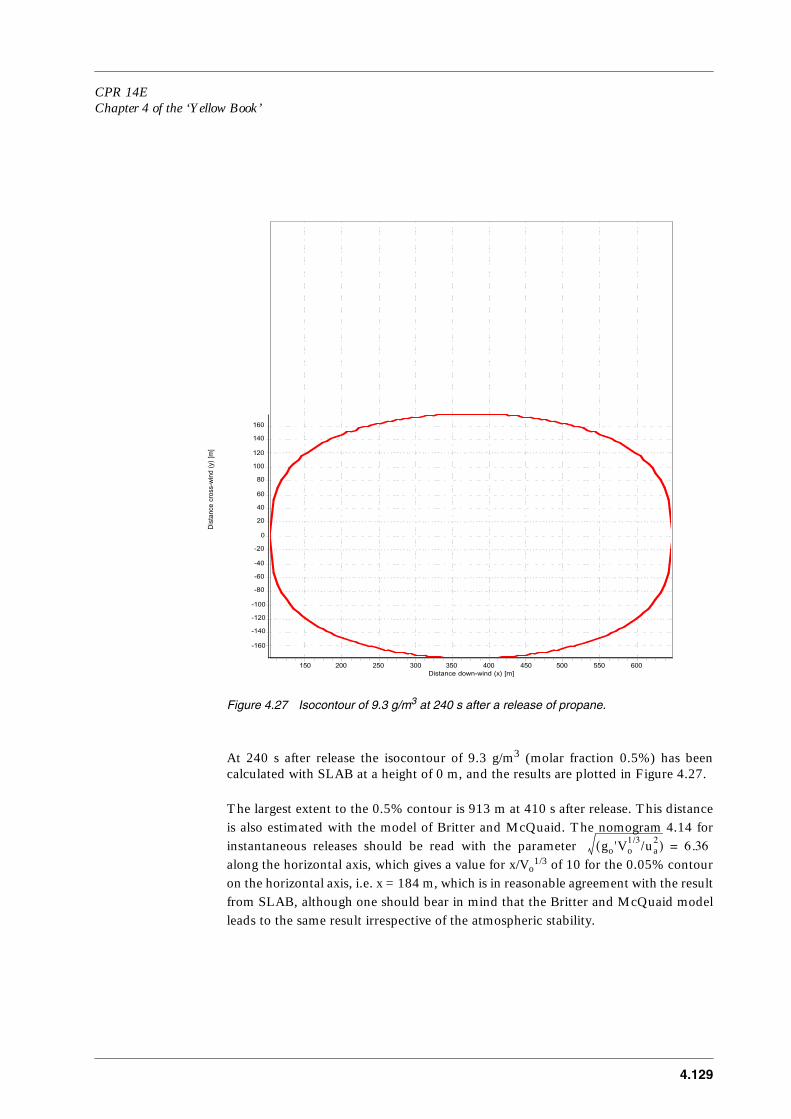
CPR 14EChapter 4 of the ‘Yellow Book’
4.129
Figure 4.27 Isocontour of 9.3 g/m3 at 240 s after a release of propane.
At 240 s after release the isocontour of 9.3 g/m3 (molar fraction 0.5%) has beencalculated with SLAB at a height of 0 m, and the results are plotted in Figure 4.27.
The largest extent to the 0.5% contour is 913 m at 410 s after release. This distanceis also estimated with the model of Britter and McQuaid. The nomogram 4.14 forinstantaneous releases should be read with the parameter along the horizontal axis, which gives a value for x/Vo
1/3 of 10 for the 0.05% contouron the horizontal axis, i.e. x = 184 m, which is in reasonable agreement with the resultfrom SLAB, although one should bear in mind that the Britter and McQuaid modelleads to the same result irrespective of the atmospheric stability.
Distance down-wind (x) [m]600550500450400350300250200150
Dis
tanc
e cr
oss-
win
d (y
) [m
]
160
140
120
100
80
60
40
20
0
-20
-40
-60
-80
-100
-120
-140
-160
go 'Vo1/3/ua
2( ) 6.36=

4.130
4.7 Discussion
4.7.1 Introduction to Section 4.7
This section provides additional information on limitations of selectedmodels, alternative solutions, and gaps of knowledge at present.
4.7.2 Changes in atmospheric conditions
Both the Gaussian plume model as the selected dense gas dispersion modeldescribe dispersion for stationary atmospheric conditions. The models are not ableto describe phenomena during changes in the boundary layer meteorology, such aspassage of fronts, diurnal variation of wind speed and wind direction near coasts, etc.As the meteorological conditions change continuously, the total travel time for whichthe models are valid needs to be maximised to about 3 hours. The maximum traveldistance is thus about 104 . ua m. For larger distances use needs to be made ofdedicated long range dispersion models.
4.7.3 Still air
Gaussian plume models are normally excluded for use in still air. Byminimising σv in formula (4.49) the range of applicability is extended compared toconventional Gaussian plume models. This minimum value of σv is probably small,thus conservative from a point of view of maximum concentration.For continuous releases during very low wind speed for which ua < 2 . σv,accumulation of plume material at the source will appear (upwind dispersion by windfluctuations becomes of the same order of magnitude as down-wind convection bywind speed), and the source need to be treated as a series of instantaneous releaseswhere σx is calculated (also in the surface layer) by formula (4.61d), and the argumentua .t in the function Fz (ua . t, z) is replaced by x for surface layer releases.
4.7.4 Accuracy of the Gaussian plume model
In Figure 4.6 regions of atmospheric conditions are indicated. The use ofthe Gaussian plume model is well assessed for the ‘near neutral upper layer’. Asdiscussed in Section 4.3.2, vertical dispersion in the surface layer, although notstrictly Gaussian, is also well understood.Dispersion in the ‘mixed layer’ and ‘free convection layer’ is proven to be notGaussian in nature. For the ‘local scaling layer’, ‘z-less scaling layer’, and‘intermittency layer’ no alternative for Gaussian plume modelling has been suggestedso far.The Gaussian plume model will at best have an accuracy of a factor of 2 for the nearneutral upper layer [Olesen et al., 1992].
CPR 14EChapter 4 of the ‘Yellow Book’
4.131
4.7.5 Dispersion over obstacles
Neither the Gaussian plume model, jet and plume models, nor the densegas models as presented in the previous sections allow predictions to be made whichtake into account the effects of obstacles. It is not allowed to introduce obstacle effectsby increasing the roughness length for the calculation: in effect, the height of thecloud should always exceed (except for very near to the source) the roughness lengthby an order of magnitude. As discussed in Section 4.2.7, effects of obstacles shouldbe taken into account if the smaller value of height or width of the obstacle(s) is largerthan the local cloud height.
Obstacle effects can be treated in a few ways. For passive dispersion some simplemodels exist for dispersion in the wake of single buildings for which the ratio of width-to-height does not exceed about 5 [Duijm and Webber, 1993]. These models assumea uniform distribution of concentration in the wake of a building. However,differences of a factor 10 are often observed.Some progress is being made in developing simple models for (dense) gas dispersionover simple obstacle arrays, such as fences perpendicular to the wind, uniformlydistributed blocks, and ‘street-canyon’ like situation [Duijm and Webber, 1993; VDI,1990].
For situations for which no such specific ‘simple’ model exists, one needs to use eitherphysical modelling by means of atmospheric boundary-layer wind or water tunnels,or computational fluid dynamic codes (CFD). For passive dispersion in near neutralconditions, for which plume rise or plume descent is not relevant, wind tunnelsimulations are as yet unsurpassed for costs and accuracy.For buoyant or dense releases, additional scaling parameters need to be used in windtunnels which lead to compromises between viscous effects and density effects. Theseeffects need to be assessed carefully for each case.CFD-modelling as yet needs approximations with respect to the representation ofturbulence. Here again these approximations should be assessed carefully for eachcase, the situations with stable stratification (either atmospheric or from the dense gascloud) being the most critical.
4.7.6 Concentration fluctuations
The selected models account for different averaging-times and‘instantaneous’ lateral plume widths. These plume widths need to be considered asso-called ensemble-averaged width and these calculations do not exclude fluctuationsof plume width and concentrations to occur.The last decade much attention has been paid to develop general models that describeconcentration fluctuations (or at least statistics of concentration fluctuations) inpassive and dense gas clouds and plumes.As yet no generalised model for concentration fluctuations is available. There isevidence that quantities of instantaneous dense and passive releases, such as dose andmaximum concentration, are log-normally distributed over the ensemble ofrealisations. For continuous releases less definite conclusions with respect todistribution functions can be given, partly because here intermittency masks part ofthe observations.
4.132
4.7.7 Removal processes
In Sections 4.2.8 and 4.2.9 some attention is paid to chemical reactions anddeposition, respectively. The selected models do not account for these processes. Forslow chemical reactions and wet deposition, one may write a first order decrease ofmaterial in the plume:
where q (x) is the source strength to be used in the (Gaussian) plume model atdistance x, and C some constant, depending on the chemical reaction or the wash-out rate.For dry deposition at the ground one may calculate the total flux by integration of(4.5) over the plume width and decrease q (x) in the plume model by this loss ofmaterial (source depletion model). However, dry deposition will affect theconcentration near the ground, thus changing the vertical distribution of material. Amodel to describe this phenomenon was developed by Rao [1981]. Although notstrictly correct, it provides sufficiently accurate predictions for practical values ofdeposition velocities and wind speeds [Bakkum, 1993].
d q x ( )
dx----------------
C q (x)–= (4.175)(kg/(m ⋅ s)) ◊

CPR 14EChapter 4 of the ‘Yellow Book’
4.133
4.8 Literature
Bakkum, E.A. (1993),Een numeriek algoritme voor de berekening van droge depositie en uitwassing van emissies in de atmosfeer (in Dutch),TNO-IMET report 93-211..
Beals G.A., (1971)Guide to local diffusion of air pollutants, tech. report 214 Weather Services USAF, NTIS, AD 726984.
Beljaars, A.C.M., A.A.M. Holtslag (1990),A software library for the calculation of surface fluxes over land and sea, Environmental software,
5
, pp 60-68.
Bianconi, R., M. Tamponi (1993),A mathematical model of diffusion from a steady source of short-duration in a finite mixing layer,Atmospheric Environment
27A
, pp 781-792,
Blackmore D.R. et al. (1982),Heavy gas dispersion models,Journal of Hazardous Materials 6 (1982) 107.
Briggs, G.A. (1969),Plume rise,U.S. Atomic Energy Commission Report TID-25075.
Britter, R.E. and McQuaid, J. (1988),Workshop on the dispersion of dense gases,HSE Contract Research Report No 17.
A.J. Byrne, S.J. Jones, S.C. Rutherford, G.A. Tickle, D.M. Webber (1992),
Description of ambient atmospheric conditions for the computer code DRIFT
,
SRD/HSE R553, SRD, Culcheth, U.K.
Chatwin P.C. (1968), The dispersion of a puff of passive contaminant in the constant stress region, Quart. J. R. Met. Soc., 94, pp. 350-360.
Chen, C.J. and Rodi, W. (1980),Vertical turbulent buoyant jets,Pergamon Press, Oxford.
Colenbrander, G.W. (1980),A mathematical model for the transient behaviour of dense vapour clouds,3rd Int. Symp. on Loss Prevention and Safety Promotion in the Process Industry (Basle).

4.134
Commissie TNO voor het onderzoek ten dienste van het Milieubeheer (1976)Modellen voor de berekening van de Verspreiding van Luchtverontreiniging, Staatsuitgeverij 1976.
Cox, R.A., and Carpenter, R.J. (1979),Further developments of a dense vapour cloud dispersion model for hazard analysis,Proceedings of the symposium on heavy gas dispersion, Frankfurt.
Davidson, G.A. (1989),Simultaneous trajectory and dilution predictions froma simple integral plume model,Atmospheric Environment 23, 341.
Deaves, D.M. (1992),Dense gas dispersion modelling,Journal of loss prevention in the process industry 4 (1992) 219.
Drivas P.J. and Shair F.H. (1974), Dispersion of an instantaneous crosswind line source of tracer released from an Urban highway, Atm. Env. 8, pp. 475-485.
Duijm, N.J., Webber, D.M (1993 or 1994),Dispersion in the presence of buildings, Problem Clouds - II, April 15/16, 1993, Amsterdam, The Netherlands and accepted for publication in J. of Los Prevention in the Process Industries, 1993 or 1994.
Eidsvik, K.J. (1980),A model for heavy gas dispersion in the atmosphere,Atmospheric Environment 14, 769.
Erbrink, J.J. (1991),A practical model for the calculation of
σ
y
and
σ
z
for use in an on-line Gaussian dispersion model for tall stacks, based on wind fluctuations,Atm. Env.,
25A
, 2, pp 277-283.
Ermak, D.L. et al. (1982),A comparison of dense gas dispersion model simulations with Burro series LNG spill test results,Journal of Hazardous Materials 6 (1982) 129.
Ermak, D.L., Rodean, H.C., Lange, R. and Chan, S.T. (1988),A survey of denser-than-air atmospheric dispersion models,LLNL Report under contract W-7405-ENG-48.
Ermak, D.L. (1990),User’s manual for SLAB: an atmospheric dispersion model for denser-than-air releases, Lawrence Livermore National Laboratory, California 94550.
CPR 14EChapter 4 of the ‘Yellow Book’
4.135
Fryer, L.S. and Kaiser, G.D. (1979),DENZ, a computer program for the calculation of the dispersion of dense toxic or explosive gases in the atmosphere,Report UKAEA SRD R/52.
Golder, D. (1972),Relations among stability parameters in the surface layer,Boundary-Layer Met.,
3
, pp 47-58.
Gryning, S.E., A.A.M. Holtslag, J.S. Irwin, B. Sivertsen (1987),Applied Dispersion modelling based on meteorological scaling parameters, Atmospheric Environment
21
/1, pp 79-89.
Guinnup, D. (1992),Non-buoyant Puff and Plume Dispersion Modelling Issues,Plant/Operations Progress
11
/1, pp 12-15.
Hanna S.R., Briggs G.A. en Hosker Jr. R.P. (1982), Handbook of Atmospheric Diffusion, DOE/TIC-11223 (DE 82002045), 1982.
Hanna, S.R. and Drivas, P.J. (1987),Guidelines for the use of vapor cloud dispersion models,CCPS American Institute of Chemical Engineers New York.
Hanna, S.R., Strimaitis, D.G., and Chang, J.C. (1991),Evaluation of commonly-used hazardous gas dispersion models,Final Report under contract FO8635-89-C-0136,Sigma Research Corporation, Concord.
Hanna, S.R. (1990),Lateral Dispersion in Light Wind Stable Conditions, Proceedings of the EURASAP Meeting and GNFAO/CNR Workshop on Atmospheric Dispersion in Low Wind speeds and Foggy Conditions, Torino, Sept. 5-7, 1989, ed. D. Anfossi & A. Longhetto, Il Nuova Cimento della società italiana di fisica vol. 13 C, num. 6,pp. 889-894.
Hanna, S.R. and Chang, J.C. (1992),Evaluation of commonly-used hazardous gas dispersion models,Addition of the HGSYSTEM model,Final Report A232-300, Sigma Research Corporation, Concord.
Havens, J. (1989),DEnse GAs DISpersion version 2.1.
Havens, J. and Spicer, T. (1990),TECJET: An atmospheric dispersion model,Risk Analysis 10 (1990) 459.

4.136
Havens, J. (1992),Review of dense gas dispersion field experiments,Journal of loss prevention in the process industry 1 (1992) 28.
Holtslag, A.A.M. (1984),Estimates of diabatic wind speed profiles from near-surface weather observations, Boundary-Layer Meteorology
29
, pp 225-250.
Holtslag, A.A.M., and F.T.M. Nieuwstadt (1986),Scaling the atmospheric boundary layer,Boundary-Layer Meteorology
36
, pp 201-209.
Holtslag, A.A.M. (1987),
Surface fluxes and boundary layer scaling - model and applications
,
KNMI WR-no 87-2, De Bilt.
Holtslag, A.A.M., and H.A.R. de Bruin (1987),Applied modelling of the night-time surface energy balance over land, submitted to J. of Climate and Applied Meteor.
Hoot, T.G., Meroney, R.N. and Peterka, J.A. (1973),Wind tunnel tests of negatively buoyant plumes,NTIS Report PB-231-590.
Hsu, S.A. (1992),An overwater stability criterion for the offshore and coastal dispersion model (research note), Boundary-Layer Met.,
60
, pp 397-402.
Jagger, S.F. (1983),Development of CRUNCH: a dispersion model for continuous releases ofdenser-than-air vapour into the atmosphere,Report UKAEA SRD R 229.
Jones, S.J., Mercer, A., Tickle, G.A., Webber, D.M. and Wren, T. (1991),Initial verification and validation of DRIFT,Report SRD/HSE/R580.
Kaiser, G.D. and Walker, B.C. (1978),Releases of anhydrous ammonia from pressurised containers and the importance of denser than air mixtures,Atmospheric Environment 12, 2289.
KNMI (1974), Luchtverontreiniging en Weer, Staatsuitgeverij, The Hague.
KNMI (1979),Luchtverontreiniging en weer, 2e druk,Staatsuitgeverij, ’s Gravenhage.

CPR 14EChapter 4 of the ‘Yellow Book’
4.137
Li, X., Leijdens, H. and Ooms, G. (1986),An experimental verification of a theoretical model for the dispersion of a stack plume heavier than air,Atmospheric Environment 20.
McFarlane, K., Prothero, A., Puttock, J.S., Roberts, P.T. andWitlox, H.W.M. (1990),Development and validation of atmospheric dispersion models for ideal gases and hydrogen fluoride,Technical Reference Manual Shell Reseach Report TNER.90.015.
Mercer, A. et al. (1993),Comparison of heavy gas dispersion models for instantaneous releases,to be published in Journal of Hazardous Materials (1993).
Olesen, H.R., T. Mikkelsen, eds (1992),
Proceedings of the workshop Objectives for Next Generation of Practical Short-Range Atmospheric Dispersion Models
,
NERI, Roskilde, Denmark.
Ooms, G. (1972),A new method for the calculation of the plume path of gases emitted by a stack,Atmospheric Environment 6, 899.
Ooms, G. and Duijm, N.J. (1984),Dispersion of a stack plume heavier than air,IUTAM Symposium, Springer Verlag.
Panofsky, H.A., and J.A. Dutton (1984),
Atmospheric Turbulence
, John Wiley & Sons, New York.
Pasquill F. and Smith F.B., (1983)Atmospheric Diffusion, Ellis Horwood Ltd., Chichester.
Pasquill, F. and F.B. Smith (1983),
Atmospheric Diffusion
, 3rd ed., Ellis Horwood, Chichester.
Peterson, R.L. (1978),Plume rise and dispersion for varying ambient turbulence, thermal stratification and stack exit conditions,PhD Thesis, Colorado State University.
Press, W.H. et al. (1986),Numerical Recipes – The Art of Scientific Computing, Cambridge University Press, Cambridge.
Puttock, J.S. et al. (1991),Dispersion models and hydrogen fluoride predictions,Journal of loss prevention in the process industry 4 (1991) 16.
4.138
Rao, K.S. (1981),Analytical solutions of a gradient-transfer model for plume deposition and sedimentation,NOAA technical memorandum ERL-ARL-109, NTIS, U.S. Dept. of Commerce. PB 82-215153.
Radian Corporation (1988),Description of the Radian complex hazardous air release model.
Saffman P.G. (1962), The effect of wind shear on horizontal spread from an instantaneous ground source, Quart. J. R. Met. Soc., 88, pp. 382.
Seinfeld, J.H. (1986),
Atmospheric Chemistry and Physis of Air Pollution
,John Wiley & Sons, New York.
Slade D.H. (1968), Meteorology and Atomic Energy, U.S. Atomic Energy Commission.
Singer, I.A., Smith, M.E. (1953),J. Meteorol.,
10
, 2, pp 92-114.
Stern, A.C., R.W. Boubel, D.B. Turner, D.L. Fox (1984),
Fundamentals of Air Pollution
,2nd ed., Academic Press, London.
Stull, R.B. (1988),
An Introduction to Boundary Layer Meteorology
,Atmospheric Sciences Library, Kluwer Academic Publishers, Dordrecht.
Tyldesley J.B. and Wallington C.E. (1965),The effect of wind shear and vertical diffusion on horizontal dispersion, Quart. J. R. Met. Soc., 91, pp. 158-174 (1965).
Ulden, A.P. van, and A.A.M. Holtslag (1985),Estimation of Atmospheric Boundary Layer Parameters for Diffusion Applications, Journal of Climate and Applied Meteorology,
24
, pp 1196-1207.
Ulden, A.P. van (1991),A surface-layer similarity model for the dispersion of a skewed passive puff near the ground, Atmospheric Environment
26A
/4, pp 681-692.
VDI Richtlinie 3783 Blatt 2 (1990),Ausbreitung von storfallbedingten Freisetzungen schwererGase - Sicherheitsanalyse,Beuth Verlag GmbH, Berlin.
CPR 14EChapter 4 of the ‘Yellow Book’
4.139
Webber, D.M. et al. (1992),A model of a dispersing dense gas cloud, and thecomputer implementation DRIFT,UKAEA Report SRD/HSE R586-587.
Werkgroep Verspreiding Luchtverontreiniging (1984),Parameters in the long-term model ofair pollution Dispersion - New recommendations,TNO-SCMO, P.O. Box 186, 600 AD Delft, The Netherlands.
Wheatley, C.J. and Webber, D.M. (1984),Aspects of the dispersion of denser-than-air vapours relevant togas cloud explosions,Final Report SR/007/80/UK/H UK Atomic Energy Authority.
Witlox, H.W.M. et al. (1990),HGSYSTEM user/technical manuals,References to chapter 4, Vapour Cloud Dispersion.
Zeman, O. (1982),The dynamics and modelling of heavier-than-air cold gas releases,Atmospheric Environment 16, 741.
CPR 14EChapter 4 of the ‘Yellow Book’
appendix
4.1-1
Appendix 4.1 A method for estimating the solar elevation
A4.1 The Julian day number
The Julian day number, J
n
, can be defined as the number of days elapsedsince the first of January.
For a date of the form DD-MM-YYYY, YYYY is first examined to see if it is a leapyear.
The following table is used for the calculation
J
n
= DD + X
MM-1
(a1.1)
in non-leap years, and up to February in all years, and
J
n
= DD + X
MM-1
+ 1 (a1.2)
in leap years after February.
A4.2 The solar elevation
In this section, all arguments of goniometrical functions are in radians.From J
n
the solar longitude (SL) can be evaluated by,
SL = 4.871 + 0.0175 J
n
+ 0.033 sin(0.0175 J
n
) (rad) (a1.3)
where SL is in radians. The solar declination (SD) follows from
SD = arc sin(0.398 sin(SL)) (rad) (a1.4)
These three quantities are used to compute the smallest angle through which theearth must turn to bring the meridian of the given location directly under the sun
MM 1 2 3 4 5 6 7 8 9 10 11 12
Jan Feb Mar Apr May Jun Jul Aug Sep Oct Nov Dec
X 031 059 090 120 151 181 212 243 273 304 334 365
α ψwπ
180-------- 0.043 2 SL⋅( ) 0.033 0.0175Jn( ) π tu/12 1–( )⋅+sin–sin+⋅= (a1.5)
appendix
4.1-2
where
ψ
w
is the western longitude (˚W) of the location and t
u
is the universal time inhours.
the solar elevation,
χ
, is given in radians by:
where
ϕ
is the latitude of the location (˚N). This scheme provides an estimate for
χ
with an accuracy of within 0.05 rad.
χ arc SD( ) ϕπ
180--------
SD( ) ϕπ
180--------
α( )cos⋅cos⋅cos+sin⋅sin
sin= (a1.6)

5.1
Chapter 5Vapour cloud explosionsW.P.M. Mercx, A.C. van den Berg

CPR 14EChapter 5 of the ‘Yellow Book’
5.3
Modifications to Chapter 5 (Vapour cloud explosions)with respect to the first print (1997)
Numerous modifications were made concerning typographical errors. A list is givenbelow for the pages on which errors have been corrected.
At page 5.24: the declaration of variable EmTNT (TNT blast energy) is corrected,and values currently in use for this variable are added.
In the calculation examples of the application of selected methods: calculationexamplesA lot of numbers are refined, and values are more accurately read from plots andfigures. The values of Tables 5.6, 5.7A, 5.7B have been replaced by refined values.

5.4
CPR 14EChapter 5 of the ‘Yellow Book’
5.5
List of symbols Chapter 5
Af,rainout Jet cross-section after flashing and rainout (5.10) m2
aa Speed of sound in ambient air (5.4) m⋅s-1
bf,rainout Jet radius after flashing and rainout (5.10) mbi Dimension of a box mcp Specific heat at constant pressure J⋅kg-1⋅K-1
cs Stoichiometric concentration (5.7) %D1 Smallest dimension of obstacle perpendicular to flame
propagation direction mD2 Dimension of obstacle parallel to flame propagation
direction mdc Diameter of a cylinder mds Diameter of a sphere mE Total combustion energy (5.2) JEm Combustion energy per unit mass (5.1) J⋅kg-1 Emf Combustion energy of fuel per unit mass (5.1) J⋅kg-1 EmTNT Combustion energy of TNT per unit mass (5.1) J⋅kg-1 Ev Combustion energy per unit volume (5.9) J⋅m3
is Positive side-on impulse of blast-wave (5.6) Pa⋅sPsc Overpressure in vapour cloud PaPs Peak side-on overpressure of blast-wave (5.3) PaPs' Scaled peak side-on overpressure of blast-wave (5.3) -pa Ambient pressure (5.2) Papdyn Peak dynamic pressure in blast-wave (5.5) Pa pdyn' Scaled dynamic pressure in blast-wave (5.5) -pCJ ‘Chapman-Jouguet’ peak detonation pressure Pa pvN ‘Von Neumann’ peak detonation pressure Pa Qex Mass quantity of flammable part of the cloud (5.7) kgQf Mass of fuel involved (5.1) kg QTNT Equivalent mass of TNT (5.1) kg r Distance to explosion centre (5.2) mr' Scaled distance (5.2) -ro Radius of flammable cloud (5.9) m ro' Scaled radius of flammable cloud -Te Temperature of combustion products KTi Temperature at start of combustion KTa Ambient temperature Ktp Positive phase duration of blast-wave (5.4) stp' Scaled positive phase duration of blast-wave (5.4) -V Volume m3
Vc Volume of vapour cloud at stoichiometricconcentration (5.8) m3
Vgr Volume of vapour within obstructed region (5.8) m3
Vo Volume of unobstructed part of the cloud (5.8) m3
Vr Free volume of the obstructed region m3
αe TNT equivalency based on energy (5.1) -αm TNT equivalency based on mass (5.1) -ρ Density (5.7) kg/m3
Note: the numbers between brackets refer to equations.

5.6

CPR 14EChapter 5 of the ‘Yellow Book’
5.7
Glossary of terms
blast (wave) a rapidly propagating pressure or shock-wave inatmosphere with high pressure, high density andhigh particle velocity
burning velocity the velocity of a propagating flame, measuredrelative to the unburnt gases immediately aheadof the flame front
deflagration a propagating chemical reaction of a substance inwhich the propagation of the reaction front isdetermined by conduction and moleculardiffusion
detonation a propagating chemical reaction of a substance inwhich the propagation of the reaction front isdetermined by compression beyond the auto-ignition temperature
explosion a sudden release of energy that causes a blast
flammable limits the upper and lower concentration limit ofcombustible material in a homogeneous mixturewith a gaseous oxidiser that will propagate aflame
impulse a measure used to quantify the consequences ofa short duration pressure pulse. It is calculatedby integration of the pressure-time history
laminar flame propagation propagation of a flame in a laminar flow,characterised by a very thin flamefront with asmooth surface that can be curved
pressure wave rapidly propagating wave in atmosphere causinga gradual change in gas-dynamic-state: highdensity, pressure and particle velocity
separation distance the minimal distance between two congestedareas at which the areas can be considered as twoseparate explosion sources
shock-wave rapidly propagating wave in atmosphere causinga instantaneous change in gas-dynamic-state:high density, pressure and particle velocity
side-on overpressure the pressure experienced by an object as a blast-wave passes by
5.8
stoichiometric ratio the ratio characterised by, or being, a proportionof chemicals exactly right for a combustion withno excess of flammable material or oxygen
TNT-equivalence the amount of TNT (trinitrotoluene) that wouldproduce observed damage levels similar to thoseof the explosion under consideration
turbulent flame propagation propagation of a flame in a turbulent flow,characterised by a rough combustion zone ratherthan by a thin and smooth flame front
vapour cloud explosion the explosion resulting from an ignition of apremixed cloud of flammable vapour, gas orspray with air, in which flames accelerate tosufficiently high velocities to produce significant overpressure
volume blockage fraction the ratio of the volume of the obstructed areaoccupied by obstacles to the total volume of theobstructed area itself

CPR 14EChapter 5 of the ‘Yellow Book’
5.9
Table of contents Chapter 5
Modifications to Chapter 5, Vapour cloud explosions .........................3
List of symbols Chapter 5 ......................................................................5
Glossary of terms ...................................................................................7
5 Vapour cloud explosions......................................................................115.1 Introduction .................................................................................115.2 The phenomenon of a vapour cloud explosion................................13
5.2.1 Introduction to vapour cloud explosions ...............................135.2.2 Combustion modes .............................................................155.2.3 Ignition ...............................................................................195.2.4 Gas explosion mechanism....................................................195.2.5 Deflagration to detonation transition (DDT) ........................205.2.6 Blast ...................................................................................21
5.3 General overview of existing vapour cloud explosion blast models..........................................................................................235.3.1 Introduction to section 5.3...................................................235.3.2 Methods based on TNT charge blast....................................235.3.3 Methods based on fuel-air charge blast .................................26
5.4 Selection of a model ......................................................................295.5 Description of model.....................................................................33
5.5.1 Introduction to the Multi-Energy concept ............................335.5.2 Discussion...........................................................................395.5.3 Procedure for the division of an area into obstructed and
unobstructed regions ...........................................................445.5.4 Procedure for the application of the Multi-Energy
method ...............................................................................465.6 Application of selected models: calculation examples ......................53
5.6.1 Introduction to section 5.6...................................................535.6.2 Definition of an obstructed region ........................................535.6.3 Vapour cloud explosion .......................................................605.6.4 Determination of obstructed region......................................65
5.7 Interfacing to other models ............................................................755.8 Literature......................................................................................77

5.10
CPR 14EChapter 5 of the ‘Yellow Book’
5.11
5 Vapour cloud explosions
5.1 Introduction
One of the physical phenomena that may occur after the accidental releaseof dangerous goods is a vapour cloud explosion. A vapour cloud can be created byeither the release of a gas from a containment or by the evaporation of a liquid thatwas released from a containment. A ‘Source Term’ calculation, in most casesfollowed by a ‘Dispersion’ calculation, will be performed usually prior to a ‘VapourCloud Explosion’ calculation.
Not all gases or vapours are flammable and if they are, they are not flammable underall circumstances. If however, the vapour cloud is flammable, or part of the cloud isflammable, a vapour cloud explosion may occur. At least, the cloud will burn after itis ignited. Other conditions described in this chapter are required to turn the burn ofa cloud into a devastating explosion.
The phenomenon of a ‘Vapour Cloud Explosion’ (VCE) is described in this chapter.An ‘effect’ model for the determination of the ‘blast’ resulting from a VCE is selected,described and elucidated with some examples. Results of this vapour cloud explosionblast model can be used as input to subsequent consequence models for thedetermination of damage to structures and injury to people. These models can befound in CPR-16E [1990].
The phenomenon of a vapour cloud explosion is presented in section 5.2. There, alsobasic features of vapour cloud explosions are explained.Knowledge of the basic features and the explosion phenomenon is necessary to selecta model for blast prediction.
Section 5.3 describes the existing models for vapour cloud explosion blast predictionand a discussion is presented regarding advantages and disadvantages of groups ofmodels. After having motivated the preference for a specific group of models, onemodel out of this group is selected in section 5.4.
The model is presented by discussing the underlying physical features in section 5.5.There, also model deficiencies and available guidance to cover these deficiencies arediscussed. Recommendations are made to cover deficiencies in a safe andconservative approach. Two procedures are presented, one for the determination ofobstructed regions and one for the application of the Multi-Energy method.
The concept of the Multi-Energy method is generally accepted as the practical modelrepresenting best the mechanics of an unconfined vapour cloud explosion. Theapplication in practice though is hampered due to the lack of appropriate guidancefor application as some aspects are still not yet fully described due to the lack ofexperimental data.Current internationally performed research aims at, amongst other things, improvingpractical prediction models and derivation of guidance for application. Additionalinformation will become available from the EU sponsored projects MERGE(Modelling and Experimental Research into Gas Explosions) and EMERGE

5.12
(Extended MERGE). The project GAME (Guidance for the Application of theMulti-Energy method) and its successor GAMES (GAME Second phase) willprovide valuable information for estimating the class of the source strength.Additional research should however be initiated to obtain knowledge on separationdistances between obstructed regions.
As this information is not available presently it is advised to choose a source strengthclass number 10. The result will be conservative as the class number is lower in almostall cases. The result will be better in comparison with the TNT equivalency methodas the basic mechanism of a gas explosion is recognised, to wit: pressure is generatedonly in those areas where the flame is accelerated by turbulence generated by theinteraction of the expansion flow ahead of the flame and obstacles present in the flamepath.
Examples for becoming familiarised with the procedures are presented in section 5.6.
The last section deals with interfacing to other models (section 5.7).

CPR 14EChapter 5 of the ‘Yellow Book’
5.13
5.2 The phenomenon of a vapour cloud explosion
5.2.1 Introduction to vapour cloud explosions
Major industrial accidents like the explosion at the caprolactam plant ofNypro Ltd in Flixborough (United Kingdom) on June 1, 1974 and the explosion atthe naphtha cracking unit of DSM in Beek (The Netherlands) on September 15,1975 demonstrate the enormous impact VCE’s can have.These two examples are often quoted to give an impression of a typical VCE as theyare well-known and well-documented. Although these two major accidents occurredseveral years ago, this does not imply that VCE’s are ruled out due to the enormousamount of safety precautions that have been developed and implemented since then.More recent accidents include Celanese (1987), Shell (1988), Phillips (1989) andExxon (1989) in the USA and Total (1991) near Marseille in France. The lastcausing window pane breakage at a distance of more than four kilometres.
All VCE’s result from the ignition of a flammable cloud which was formed due to therelease of a large quantity of flammable vaporising liquid or gas from a storage tank,a process or transport vessel, or a pipeline. However, not all of these releases will necessarily lead to a VCE.Generally speaking, several conditions need to be present for a vapour cloudexplosion with damaging overpressure to occur.
First, the released material must be flammable and at suitable conditions of pressureor temperature. Examples of suitable materials are liquefied gases under pressure(propane, butane), ordinary flammable liquids particularly at high temperatures and/or pressures (cyclohexane, naphtha), and non-liquefied flammable gases (methane,ethene, acetylene).
Secondly, a cloud must be formed prior to ignition (dispersion phase). Should ignitionoccur instantly at the release, a flare - in itself causing extensive localised heatradiation damage - will occur. However, significant blast pressures causingwidespread damage are not likely to occur. Should the cloud be allowed to form overa period of time within a process area and subsequently ignite, blast pressurespropagating away from the cloud centre can result in extensive damage over a widearea. Ignition delays from one to five minutes are considered the most probable ofgenerating a vapour cloud explosion, although major incidents with ignition delays aslow as a few seconds and higher than 30 minutes have been documented.
Thirdly, a part of the cloud must be within the flammable range of the material. Avapour cloud will generally have three regions - a rich region near the point of release,a lean region at the edge of the cloud and a region in between that is within theflammable range. The percentage of the vapour cloud in each region varies,depending on a great deal of different factors, including type and amount of thematerial released, pressure at release, size of release opening (all of them sourceterms), degree of confinement of the cloud, and wind, humidity and otherenvironmental effects [Hanna and Drivas, 1987].
Fourthly, the blast effects produced by vapour cloud explosions are determined by thespeed of flame propagation. The faster the flame propagates through the flammable
5.14
cloud, the higher the overpressure in the cloud will be, which will increase the blasteffects outside the cloud. This implies that the mode of flame propagation is veryimportant. In general, the mode of flame propagation will be a deflagration. Underextraordinary conditions a detonation might occur.Section 5.2.2 discusses the modes of combustion in more detail.
When ignition occurs in a flammable cloud at rest, the flame will start to propagateaway from the ignition point. The combustion products expand causing flow aheadof the flame. Initially this flow will be laminar. Under laminar or near-laminarconditions the flame speeds for normal hydrocarbons are in the order of 5 to 30 m/swhich is too low to produce any significant blast overpressure. Under theseconditions, that is, should the combustion rate not be intensified, the vapour cloudwill simply burn and the event is described as a large flash fire.
Therefore, an additional condition is necessary for vapour cloud explosions withpressure development: the presence of turbulence. Research testing has shown thatturbulence will significantly enhance the combustion rate in deflagrations.
Turbulence may arise in a vapour cloud explosion accident scenario in various ways,namely:– by the release of flammable material itself, for instance a jet release or a
catastrophic failure of a vessel resulting in a explosively dispersed cloud,– by the interaction of the expansion flow ahead of the flame with obstacles present
in a congested area, for instance, in industrial installations.
Both mechanisms may cause very high flame speeds and, as a result, strong blastpressures. The generation of high combustion rates is limited to the release area or to congestedareas respectively. As soon as the flame enters an area without turbulence due to therelease, or enters an area without obstruction, the combustion rate will drop as wellas the pressure generation.Of course, both mechanisms may also occur simultaneously, as with a jet releasewithin a congested area.
In the extreme, the turbulence can cause the flame propagation mode to changesuddenly from deflagration into detonation. This mode of flame propagation isattended by propagation speeds in excess of the speed of sound (twice to 5 times thespeed of sound) and maximum overpressures of about 18 bar (18 × 105 Pa). Tomaintain its speed of propagation, turbulence is no longer necessary, which meansthat unobstructed and/or quiescent flammable parts of a cloud may also participatein the production of blast. It should, however, be emphasised that for a detonation topropagate, experimental indications suggest that the flammable part of the cloudmust be rather homogeneously mixed. For this reason a vapour cloud detonation ofthe cloud as a whole, is a most unlikely phenomenon to occur.
The likelihood of occurrence of deflagration and a detonation is also influenced bythe ignition process. Hydrocarbon-air mixtures need a high-explosive charge as theignition source for direct initiation of a detonation. Therefore, deflagrations are themost common combustion mode and detonations arise from a Deflagration toDetonation Transition (DDT).
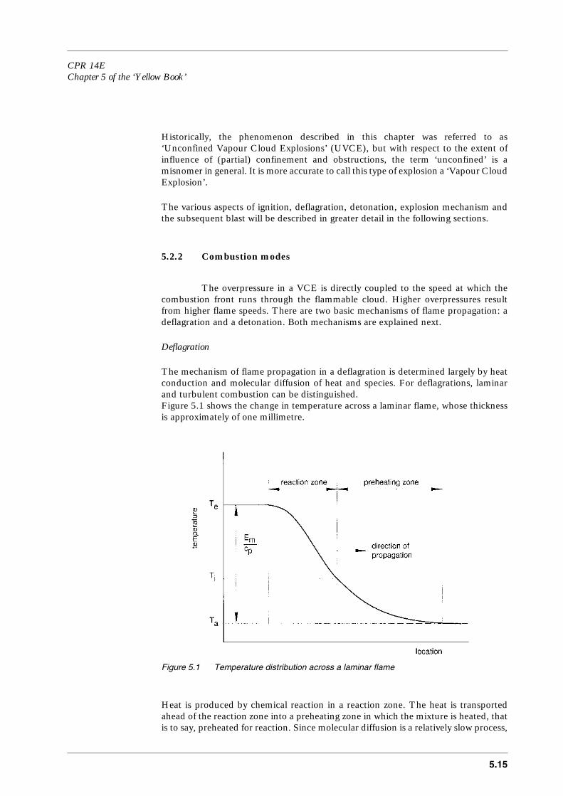
CPR 14EChapter 5 of the ‘Yellow Book’
5.15
Historically, the phenomenon described in this chapter was referred to as‘Unconfined Vapour Cloud Explosions’ (UVCE), but with respect to the extent ofinfluence of (partial) confinement and obstructions, the term ‘unconfined’ is amisnomer in general. It is more accurate to call this type of explosion a ‘Vapour CloudExplosion’.
The various aspects of ignition, deflagration, detonation, explosion mechanism andthe subsequent blast will be described in greater detail in the following sections.
5.2.2 Combustion modes
The overpressure in a VCE is directly coupled to the speed at which thecombustion front runs through the flammable cloud. Higher overpressures resultfrom higher flame speeds. There are two basic mechanisms of flame propagation: adeflagration and a detonation. Both mechanisms are explained next.
Deflagration
The mechanism of flame propagation in a deflagration is determined largely by heatconduction and molecular diffusion of heat and species. For deflagrations, laminarand turbulent combustion can be distinguished.Figure 5.1 shows the change in temperature across a laminar flame, whose thicknessis approximately of one millimetre.
Figure 5.1 Temperature distribution across a laminar flame
Heat is produced by chemical reaction in a reaction zone. The heat is transportedahead of the reaction zone into a preheating zone in which the mixture is heated, thatis to say, preheated for reaction. Since molecular diffusion is a relatively slow process,
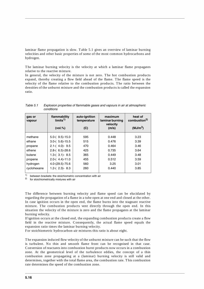
5.16
laminar flame propagation is slow. Table 5.1 gives an overview of laminar burningvelocities and other basic properties of some of the most common hydrocarbons andhydrogen.
The laminar burning velocity is the velocity at which a laminar flame propagatesrelative to the reactive mixture. In general, the velocity of the mixture is not zero. The hot combustion productsexpand, thereby creating a flow field ahead of the flame. The flame speed is thevelocity of the flame relative to the combustion products. The ratio between thedensities of the unburnt mixture and the combustion products is called the expansionratio.
Table 5.1 Explosion properties of flammable gases and vapours in air at atmospheric conditions
The difference between burning velocity and flame speed can be elucidated byregarding the propagation of a flame in a tube open at one end and closed at the other.In case ignition occurs in the open end, the flame burns into the stagnant reactivemixture. The combustion products vent directly through the open end. In thissituation the velocity of the mixture is zero and the flame propagates at the laminarburning velocity. If ignition occurs at the closed end, the expanding combustion products create a flowfield in the reactive mixture. Consequently, the actual flame speed equals theexpansion ratio times the laminar burning velocity.For stoichiometric hydrocarbon-air mixtures this ratio is about eight.
The expansion induced flow velocity of the unburnt mixture can be such that the flowis turbulent. No thin and smooth flame front can be recognised in that case.Conversion of reactants into combustion burnt products now occurs in a combustionzone. At the geometrical level of the turbulence eddies, the concept of a thincombustion zone propagating at a (laminar) burning velocity is still valid anddetermines, together with the total flame area, the combustion rate. This combustionrate determines the speed of the combustion zone.
gas orvapour
flammabilitylimits1)
(vol.%)
1) between brackets: the stoichiometric concentration with air
auto-ignitiontemperature
(C)
maximum laminar burning
velocity(m/s)
heat of combustion2)
(MJ/m3)
2) for stoichiometrically mixtures with air
methane 5.0-( 9.5)-15.0 595 0.448 3.23ethane 3.0-( 5.6)-15.5 515 0.476 3.39propane 2.1-( 4.0)- 9.5 470 0.464 3.46ethene 2.8-( 6.5)-28.6 425 0.735 3.64butane 1.3-( 3.1)- 8.5 365 0.449 3.48propene 2.0-( 4.4)-11.0 455 0.512 3.59hydrogen 4.0-(29.5)-75.6 560 3.25 3.01cyclohexane 1.2-( 2.3)- 8.3 260 0.440 3.85

CPR 14EChapter 5 of the ‘Yellow Book’
5.17
Without change in the basic mechanism of a deflagration, flame speeds can have allvalues between very low (a few metres per second) and high (more than 1000 metresper second) with accompanying increasing overpressures from a few to more than athousand kiloPascals.
Detonation
In detonative combustion the reaction front is propagated by a shock-wave whichcompresses the mixture beyond its auto-ignition temperature. At the same time, theshock is maintained by the heat released from the combustion reaction.Some basic features must be understood to understand the behaviour of a detonation.Surprisingly accurate values of overall properties of a detonation, including wavespeed and pressure, may be computed from the Chapman-Jouguet (CJ) model[Nettleton, 1987]. In this model, a detonation wave is simplified as a reactive shockin which instantaneous shock compression and the instantaneous reaction at thecombustion front coincide. For stoichiometric hydrocarbon-air mixtures, thedetonation wave speed is in the range of 1700-2100 m/s and correspondingdetonation wave overpressures are in the range of 18-22 bars (18 × 105 - 22 × 105 Pa).A slightly more realistic concept from the point of view that it reflects more than whatis actually occurring in the detonation, is the Zel’dovich-Von Neumann-Döhring(ZND) model. In this model, the fuel-air mixture does not react on shockcompression beyond auto-ignition conditions before a certain induction period haselapsed (Figure 5.2).
Figure 5.2 The ZND model for a detonation
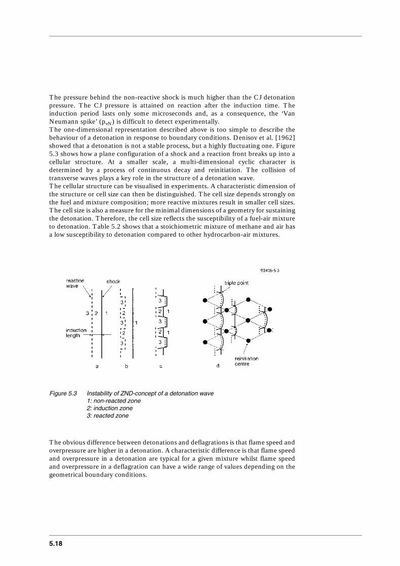
5.18
The pressure behind the non-reactive shock is much higher than the CJ detonationpressure. The CJ pressure is attained on reaction after the induction time. Theinduction period lasts only some microseconds and, as a consequence, the ‘VanNeumann spike’ (pvN) is difficult to detect experimentally.The one-dimensional representation described above is too simple to describe thebehaviour of a detonation in response to boundary conditions. Denisov et al. [1962]showed that a detonation is not a stable process, but a highly fluctuating one. Figure5.3 shows how a plane configuration of a shock and a reaction front breaks up into acellular structure. At a smaller scale, a multi-dimensional cyclic character isdetermined by a process of continuous decay and reinitiation. The collision oftransverse waves plays a key role in the structure of a detonation wave.The cellular structure can be visualised in experiments. A characteristic dimension ofthe structure or cell size can then be distinguished. The cell size depends strongly onthe fuel and mixture composition; more reactive mixtures result in smaller cell sizes.The cell size is also a measure for the minimal dimensions of a geometry for sustainingthe detonation. Therefore, the cell size reflects the susceptibility of a fuel-air mixtureto detonation. Table 5.2 shows that a stoichiometric mixture of methane and air hasa low susceptibility to detonation compared to other hydrocarbon-air mixtures.
Figure 5.3 Instability of ZND-concept of a detonation wave1: non-reacted zone2: induction zone3: reacted zone
The obvious difference between detonations and deflagrations is that flame speed andoverpressure are higher in a detonation. A characteristic difference is that flame speedand overpressure in a detonation are typical for a given mixture whilst flame speedand overpressure in a deflagration can have a wide range of values depending on thegeometrical boundary conditions.

CPR 14EChapter 5 of the ‘Yellow Book’
5.19
5.2.3 Ignition
Ignition can lead to either of the two combustion modes, deflagration ordetonation, depending on source properties. Ignition energies leading to deflagrationsare in the order of 10-4 J, whereas direct initiation of detonation requires an energy ofapproximately 106 J. Table 5.2 gives minimum ignition energies for deflagration anddetonation for some fuel-air mixtures. Considering the high energy required fordetonation, a direct initiation of a detonation is a very unlikely occurrence.In practice, vapour cloud ignition can be the result of a sparking electric apparatus orhot surfaces present in a chemical plant, such as extruders, hot steam lines or frictionbetween moving parts of a machine. Another common source of ignition is open fireand flame, for instance, in furnaces and heaters. Mechanical sparks, for example,from the friction from moving parts of a machine and falling objects, are also frequentsources of ignition. Many metal-to-metal combinations result in mechanical sparksthat are capable of igniting gas or vapour-air mixtures.In general, ignition sources must be assumed to be present in industrial installations.
Table 5.2 Characteristic detonation cell size and ignition energies for deflagration and detonation for some stoichiometric fuel-air mixtures
5.2.4 Gas explosion mechanism
Research during the last twenty-five years has revealed the mechanism bywhich a slow-burning flame is transformed into an intense blast generating processlike a vapour cloud explosion.When a flammable vapour cloud is ignited, initially a thin laminar flame with asmooth surface will start to propagate away from the ignition location. Due to theintrinsic unstable nature of a flame, flame instabilities will wrinkle the flame surface,thereby enlarging the flame surface and thus the combustion rate. This results in anincreased expansion which pushes the flame to a larger speed. Effective burningvelocities are not much higher than the laminar burning velocity, and overpressuresgenerated are in the order of some hundreds of Pascals.
Due to the expansion of the reacted products, a flow field is created ahead of theflame. If this field is disturbed, for instance due to shear layers occurring in the flowat solid boundaries or, more important, if the flow pattern is changed by the presence
fuel cell size
(mm)
minimum ignition energy for
deflagration detonation
(mJ) (mJ)
methane 300 0.28 2.3 × 10¹¹
propane 55 0.25 2.5 × 10⁹
propene 55 0.28 7.6 × 10⁸
ethene 25 0.07 1.2 × 10⁸
acetylene 10 0.007 1.29 × 10⁵

5.20
of obstacles, the shape of the flame is changed. The flame will be stretched andwrinkled, as a result its surface is enlarged and the combustion rate is increased.As more fuel is converted into combustion products per unit of volume and time,expansion flow becomes stronger. Again, the flame surface area is enlarged and thewhole process is accelerated. At a certain velocity the flow becomes turbulent and thecombustion front breaks up in a combustion zone. In a turbulent mixture combustiontakes place in an extended zone in which combustion products and unreacted mixtureare intensely mixed. High combustion rates can result because, within thecombustion zone, the reacting interface between combustion products and reactantscan become very large.Higher combustion rates produce stronger expansion, i.e. higher flow velocities withan increased level of turbulence. This process feeds on itself, a positive feedbackcoupling comes into action (Figure 5.4).
Figure 5.4 Positive feedback, the basic mechanism of a gas explosion
The obstacles and structures present in the vapour cloud, acting as turbulencegenerators, play a very important role in the development of the process. A change ofthe obstacle configuration in the flow path changes the acceleration process. Anabsence of turbulence generators will lead to a reduction in flow speed and willdecelerate the flame. Acceleration of the flame is influenced also by the measure ofobstruction and confinement of the expansion flow. Due to the restricted expansionpossibilities of the combustion products a one-dimensional flow (in a pipe) causesmore acceleration than a two-dimensional (between parallel plates) or a three-dimensional flow with no confinement at all.
5.2.5 Deflagration to detonation transition (DDT)
If the positive feedback process described in the previous paragraphcontinues to accelerate the flame, the combustion mode may suddenly changedrastically. The reactive mixture just in front of the turbulent combustion zone ispreconditioned for reaction by a combination of compression and heating byturbulent mixing with combustion products. If turbulent mixing becomes too intense,the combustion reaction may quench locally as the chemical process of combustioncan not cope with the physical process of turbulence. A very local, non-reacting buthighly reactive mixture of reactants and hot products is the result. The intensity of
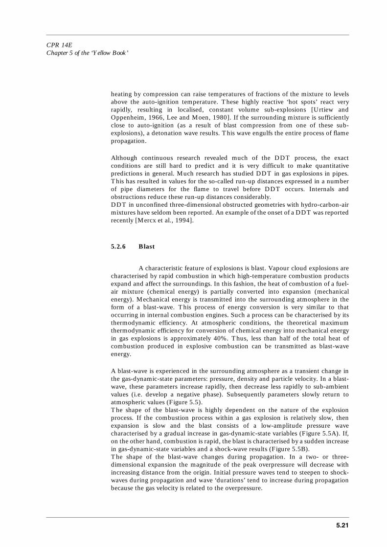
CPR 14EChapter 5 of the ‘Yellow Book’
5.21
heating by compression can raise temperatures of fractions of the mixture to levelsabove the auto-ignition temperature. These highly reactive ‘hot spots’ react veryrapidly, resulting in localised, constant volume sub-explosions [Urtiew andOppenheim, 1966, Lee and Moen, 1980]. If the surrounding mixture is sufficientlyclose to auto-ignition (as a result of blast compression from one of these sub-explosions), a detonation wave results. This wave engulfs the entire process of flamepropagation.
Although continuous research revealed much of the DDT process, the exactconditions are still hard to predict and it is very difficult to make quantitativepredictions in general. Much research has studied DDT in gas explosions in pipes.This has resulted in values for the so-called run-up distances expressed in a numberof pipe diameters for the flame to travel before DDT occurs. Internals andobstructions reduce these run-up distances considerably. DDT in unconfined three-dimensional obstructed geometries with hydro-carbon-airmixtures have seldom been reported. An example of the onset of a DDT was reportedrecently [Mercx et al., 1994].
5.2.6 Blast
A characteristic feature of explosions is blast. Vapour cloud explosions arecharacterised by rapid combustion in which high-temperature combustion productsexpand and affect the surroundings. In this fashion, the heat of combustion of a fuel-air mixture (chemical energy) is partially converted into expansion (mechanicalenergy). Mechanical energy is transmitted into the surrounding atmosphere in theform of a blast-wave. This process of energy conversion is very similar to thatoccurring in internal combustion engines. Such a process can be characterised by itsthermodynamic efficiency. At atmospheric conditions, the theoretical maximumthermodynamic efficiency for conversion of chemical energy into mechanical energyin gas explosions is approximately 40%. Thus, less than half of the total heat ofcombustion produced in explosive combustion can be transmitted as blast-waveenergy.
A blast-wave is experienced in the surrounding atmosphere as a transient change inthe gas-dynamic-state parameters: pressure, density and particle velocity. In a blast-wave, these parameters increase rapidly, then decrease less rapidly to sub-ambientvalues (i.e. develop a negative phase). Subsequently parameters slowly return toatmospheric values (Figure 5.5).The shape of the blast-wave is highly dependent on the nature of the explosionprocess. If the combustion process within a gas explosion is relatively slow, thenexpansion is slow and the blast consists of a low-amplitude pressure wavecharacterised by a gradual increase in gas-dynamic-state variables (Figure 5.5A). If,on the other hand, combustion is rapid, the blast is characterised by a sudden increasein gas-dynamic-state variables and a shock-wave results (Figure 5.5B).The shape of the blast-wave changes during propagation. In a two- or three-dimensional expansion the magnitude of the peak overpressure will decrease withincreasing distance from the origin. Initial pressure waves tend to steepen to shock-waves during propagation and wave ‘durations’ tend to increase during propagationbecause the gas velocity is related to the overpressure.
5.22
Figure 5.5 Blast-waves overpressure historiesA: pressure waveB: shock-wave
The loading of a structure due to blast depends on the interaction between the blast-wave and the structure itself as the interaction changes the blast-wave parameters.This phenomenon of explosion blast is not the subject of this chapter but is describedin detail in, for instance, CPR-16E [1990].
CPR 14EChapter 5 of the ‘Yellow Book’
5.23
5.3 General overview of existing vapour cloud explosion blast models
5.3.1 Introduction to section 5.3
Basically there are two groups of models for describing explosion blast. Thefirst group of models quantifies the source as an equivalent quantity of highexplosives, generally TNT, in order to be able to apply known TNT blastcharacteristics. Historically, these types of models are widely-used and well-accepted.During the last decade, the process of pressure development in a vapour cloudexplosion has been the subject of intense international research after discovering theimpossibility to describe some major vapour cloud explosion incidents with availablemethods at that time. This research effort resulted in methods which take intoaccount the different behaviour of a vapour cloud explosion with respect to a high-explosives detonation. This second group of models will be referred to as fuel-aircharge blast models. This type of models is being applied more and more, althoughsome lack of data hinders a general acceptation.The differences between the models in a group result from the differences in guidancein the application the concept and from differences in the used blast distancerelations.
The two groups of models are discussed in the next two sections.
5.3.2 Methods based on TNT charge blast
The military have always been interested in the destructive potential ofhigh-explosives. Consequently, the relationship between damage and high-explosiveshas been available for many years [e.g. Robinson 1944, Schardin 1954, Glasstone andDolan 1977 and Jarrett 1968]. Therefore, it is an understandable approach to relatethe explosive power of an accidental explosion to an equivalent TNT-charge. In thisway, damage patterns observed in many major vapour cloud explosion incidents wererelated to equivalent TNT-charge weights.Because the need to quantify the potential explosive power of fuels arose long beforethe mechanisms of blast generation in vapour cloud explosions were fully understood,the TNT-equivalency concept was also utilised to make predictive estimates, i.e. toassess the potential damage effects from a given amount of fuel. Basically, the use ofTNT-equivalency methods for blast predictive purposes is very simple. The availablecombustion energy in a vapour cloud is converted into an equivalent charge weight ofTNT according to:
QTNT αe
Qf × Emf
EmTNT-----------------------× αm Qf×= = (5.1)(kg)
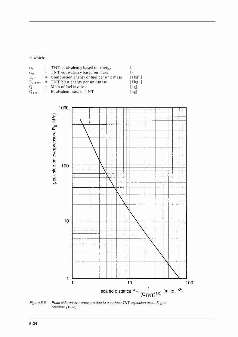
5.24
in which:
αe = TNT equivalency based on energy [-]αm = TNT equivalency based on mass [-]Emf = Combustion energy of fuel per unit mass [J⋅kg-1]EmTNT = TNT blast energy per unit mass [J⋅kg-1]Qf = Mass of fuel involved [kg]QTNT = Equivalent mass of TNT [kg]
Figure 5.6 Peak side-on overpressure due to a surface TNT explosion according to Marshall [1976]

CPR 14EChapter 5 of the ‘Yellow Book’
5.25
Values of EmTNT currently in use range from 4.19 to 4.65 MJ/kg [Brasie and Simpson,1968].The TNT-equivalency is also indicated in literature as the equivalency factor, yieldfactor, efficiency factor or efficiency.Knowing the TNT-charge weight, the blast characteristics in terms of the peak side-on overpressure of the blast-wave dependent on the distance to the charge and thecorresponding damage pattern, are known. They can be read from a chart containinga scaled graphical representation of experimental data. For this purpose various datasets are available, Figure 5.6 gives an example.
Strictly speaking, TNT-equivalency methods reduce the problem of vapour cloudexplosion blast modelling to the determination of an appropriate value for the TNT-equivalency.
Reported values for the TNT-equivalency, deduced from the damage observed inmany vapour cloud explosion incidents, range from a fraction of one per cent up tosome tens of per cent. This is reflected in the TNT-equivalence factors adopted inTNT blast charge methods.A brief overview of these methods is given next. It should to be kept in mind thatTNT-equivalence factors given have to be used with particular methods to quantifythe amount of fuel involved and with particularly mentioned TNT blast charts.All TNT-equivalence factors given are based on energy.
Brasie and Simpson [1968] and Brasie [1976]
They recommend TNT equivalencies of 2% for near-field and 5% for far-field effectsin combination with a method to quantify the amount of fuel released.
Eichler and Napadensky [1977]
Because of the distance dependency of the TNT-equivalence factor they recommend20% for the 1 psi (6.9 kPa) overpressure level only.
Health Safety Executive [1979 and 1986]
They recommend a value of 3% for gases with average reactivity (methane), 6% forabove average gases (propene oxide) and 10% for very reactive gases (ethene oxide).The mass of fuel in the cloud is taken as twice the theoretical flash of the amountreleased, in order to account for spray and aerosol formation.The maximum overpressure in the cloud is taken as 1 bar (100 kPa). The duration ofthe blast-wave should be chosen between 100 and 300 ms.
Exxon [CCPS, 1994]
Exxon provides guidance to determining the quantity of material in the cloud andadvises TNT-equivalencies of 3% for a vapour cloud covering an open terrain and10% for a vapour cloud that is partially confined or obstructed.
Industrial Risk Insurers [1990]

5.26
IRI present two credible incidents to determine the quantity of fuel in the cloud anduses a TNT-equivalence factor of 2%.
Factory Mutual Research [1990]
FMR notes that history shows TNT-equivalence factors as high as 50% but most fallin a range between 10%. Like HSE they recommend factors depending on thereactivity of the fuel involved. Factors are assigned to three classes: low-reactive 5%,average-reactive 10% and high-reactive 15%.
CPR-14E [1988]
One of the two models given in this version of the ‘Yellow Book’ relates the availableexplosion energy directly to damage circles (correlation model). In fact, this is aTNT-equivalence model. A ‘yield’ (TNT-equivalence factor) of 10% is used.
British Gas [Harris and Wickens, 1989]
Their method is intended for a non-detonating cloud of natural gas (mostlymethane). Their approach is not based on the total amount of fuel released but on themass of the material which can be contained in stoichiometric proportions in anyseverely congested region in the cloud. An overpressure of four bars (4⋅106 Pa) isassumed within the confined part. A TNT-equivalence factor of 20% should be usedfor the total congested mass. They state that the method predicts significantly lowerfar-field overpressures in cases where there is little obstruction and that in manycircumstances the possibility of VCE’s with significant overpressures can bediscounted.
Direction des etudes et Recherches, France [Van den Berg and Lannoy, 1993]
The value of the TNT equivalence factor [Van den Berg and Lannoy, 1993] has beendiscussed by Lannoy. He refers to a statistical analysis of 120 damage points of23 accidents showing a wide distribution of TNT equivalencies (0.02%-15.9%) witha medium of 3%. Of the cases 97% was covered by a TNT equivalence lower than orequal to 10% while the mean value observed was an equivalency of 4% covering 60%of the cases. He states that TNT equivalence methods for VCEs should only be usedfor the assessment of far-field blast effects where the levels are less than 30 kPa.Otherwise the methods lead to overdesigned structures. Attention is drawn to theFrench situation where the French Authority Safety Rule [1982] recommends the10% equivalency for safety factors and that the French Chemical Industry [1986]recommends the 4% equivalency, both based on the full amount of fuel released.
5.3.3 Methods based on fuel-air charge blast
So far, vapour cloud explosion blast has been modelled without consideringa major feature of gas and vapour explosions, namely, that their strength is a variable.In addition, TNT blast characteristics do not correspond properly to vapour cloudexplosion blast characteristics. This is demonstrated by the distance dependentTNT-equivalency observed in vapour cloud explosion blast. In particular, the blast

CPR 14EChapter 5 of the ‘Yellow Book’
5.27
from relatively mild (low strength) vapour cloud explosions can not be represented byTNT-blast in a satisfactory way. Therefore, the need for a blast model which reflectsmore basic gas explosion blast characteristics, was felt.
Munday [1976] developed a method to match the gas dynamics produced byspherical flame propagation to far-field TNT-blast characteristics.Baker et al. [1983] recommended the use of computational data on gas explosionblast for vapour cloud explosion blast modelling. The data were generated with theCLOUD-code. Spherical steady flame speed gas explosions were numericallysimulated [Luckritz, 1977 and Strehlow et al. 1979]. The blast effects werecondensed in a graphical representation of the distribution of the most importantblast parameters in the vicinity of a spherical fuel-air charge. The above references,however, did not give suggestions for using these tools for a predictive estimate of avapour cloud’s explosive potential. Vapour cloud explosion blast prediction methods,using fuel-air blast data, are presented next.
Wiekema [1980]
Wiekema [1980] used the gas dynamics induced by a spherical expanding piston as amodel for vapour cloud explosion blast [CPR-14E, 1988]. A piston blast model offersthe possibility to introduce a variable initial strength of the blast. This approach enables modelling vapour cloud explosion blast by considering the twomajor characteristics of gas explosion blast:– the scale, determined by the combustion energy of the total cloud inventory, and– the initial strength, determined largely by the combustion rate in the explosion
process for which three reactivity classes are defined. Some influence ofobstruction is taken into account.
Output parameters are peak overpressure and positive phase duration.
The Multi-Energy method [Van den Berg, 1985]
Experimental research during the last decade showed clearly that deflagrativecombustion generates blast only in those parts of a quiescent vapour cloud which aresufficiently obstructed and/or partially confined [Zeeuwen et al., 1983, Harrison andEyre, 1987, Harris and Wickens, 1989 and Van Wingerden, 1989].This feature is the basis of the Multi-Energy method and underlies the method ofblast modelling. Contrary to the TNT-blast models (except the one from Harris and Wickens) and themodel of Wiekema [1980], in which the contributing energy is based on the totalenergy content of the cloud, the Multi-Energy method takes into account the totalcombustion energy of those parts of the cloud that are located in obstructed and/orpartly confined areas. An obstructed area is an area where obstacles are present in aconfiguration suited to accelerate a flame if the area is engulfed by a flammable gasmixture. Each obstructed area should be treated separately as a blast source in casetheir relative separation distance is large enough. Otherwise, all the individual sourceenergies should be added and the explosion manifests itself as a single event.
An idealised gas explosion blast model was generated by computation and presentedin three non-dimensionalised graphs from which the most important parameters canbe determined (peak overpressure, positive phase duration, shape of the blast-waveand dynamic peak pressure). Steady flame speed gas explosions were numerically
5.28
simulated with the BLAST-code [Van den Berg, 1980] and their blast effects wereregistered.These blast charts should be used for calculating the blast from each explosionsource.
Although in the Multi-Energy method a fuel-air charge blast model is recommendedfor the representation of blast effects, a TNT-blast model may be used as well. It canbe demonstrated that the blast resulting from a TNT explosion with a 20% TNTequivalency of the energy will correspond closely to the blast as predicted with theMulti-Energy severest blast curve in the overpressure range of 10 to 100 kPa.Overpressure according to the Multi-Energy method will be higher in the far field dueto the specific nature of a VCE.This TNT-equivalency approach within the Multi-Energy framework, however, lacksthe basic possibilities for a further refinement in the specification of an initial blaststrength.
Shell [Cates, 1991]
Cates [1991] has proposed a methodology comparable with the Multi-Energymethod. He claims that, due to the pressure decay law used, in the Multi-Energy method,overpressures in the far-field are underpredicted by the Multi-Energy used, althoughstill higher predictions are made compared to the TNT equivalence methods. He alsoclaims that, from a comparison with experiments, the Multi-Energy methodoverestimates the near field overpressure, even if the overpressure measured in thecloud is used.As a number of questions are still unanswered a simple acoustic law is preferred todetermine peak overpressure.Another adaptation is that the volume of the cloud to be taken into account shouldbe extended to 2 m outside the obstructed region. The reason is that due to ventingof unburnt gases out of the obstructed area during combustion, part of theunobstructed volume near to the obstructed part will be very turbulent and thuscontribute to overpressure generation.A decision tree is presented to estimate a source overpressure.
Mobil Research/Baker Engineering [Baker et al., 1994]
The method of Baker et al. [1994] consists of a combination of the Multi-Energymethod and the blast curves of Strehlow [1979], with peak overpressures and impulseas output parameters. The blast curves of Strehlow were appreciated more than thoseof the Multi-Energy method because Strehlow gives a graph with curves for theimpulse. A more basic reason to choose for the Strehlow curves is that each curve isbased on a certain flame speed reached in the VCE. Based on an extensive survey of all available experimental investigations on VCE,guidance has been derived for a proper choice of the maximum flame speed to beexpected. Although a method is given to determine the source strength in terms of flame speed,still judgements and assumptions have to be made to determine the obstacle density,reactivity and flame diversion.Baker et al. [1994] provide some guidance.
CPR 14EChapter 5 of the ‘Yellow Book’
5.29
5.4 Selection of a model
TNT charge blast models
The basic assumption in TNT charge blast models, a proportional relation betweenthe amount of fuel available in the cloud and the TNT-charge weight expressing thecloud’s explosive potential, is most questionable. This is reflected by the wide rangeof equivalencies found if a large number of vapour cloud explosion incidents,involving only fuels whose heats of combustion are of the same magnitude as those ofhydrocarbons, is analysed.Nevertheless, the TNT-equivalency concept makes it possible to model the blasteffects of a vapour cloud explosion in a very simple and practical way. Theattractiveness of these methods is the very direct, empirical relation between a chargeweight of TNT and the resulting structural damage. Therefore, the TNT-equivalencyseems to be a useful tool if the property damage potential of vapour cloud explosionis the major concern.
Values for the TNT-equivalency are deduced by statistical analysis from the damageobserved in a limited number of major vapour cloud explosion incidents. For the widerange of equivalencies observed, characteristic values such as an average (4%) and anapproximate upper limit (10%) were recommended to be used for predictivepurposes. The average value is very near the TNT equivalency in the distributionwhere the majority of cases are found, i.e. an equivalency of 4% corresponds to ‘anaverage major incident’. Undoubtedly, ‘an average major incident’ represents asituation in which an accidental release of fuel is most likely such as, for instance, thesite of a refinery or chemical plant or the site of a crowded marshalling yard duringoperations. Strictly speaking, by using an average value of the TNT-equivalency,‘average major incident conditions’ are extrapolated to an actual situation. Therefore,TNT-equivalency methods give a reasonable estimate of far-field blast effects only ifthe actual conditions correspond more or less to ‘average major incident conditions’.
TNT blast is a poor model for vapour cloud explosion blast. While a TNT chargeproduces a shock-wave of a very high amplitude and a short duration, a vapour cloudexplosion produces a blast-wave, often shocks, of lower amplitude and longerduration. If the blast modelling is the starting point for the computation of structuralresponse, for instance, the design of blast resistant structures like control rooms,TNT blast will be a less satisfactorily model. Then, the shape and the positive phaseduration of the blast-wave are important parameters which should be considered andthe use of a more appropriate blast model is recommended.A practical value for TNT-equivalency is an average, based on a wide statisticaldistribution found in practice. As a consequence, a predictive estimate with TNT-equivalency on the basis of an average value has a very limited statistical reliability. Amore deterministic estimate of blast effects is possible if a parameter could be foundwhich correlates with the process of blast generation in vapour cloud explosions. In the alternative group of models, the fuel-air charge blast models, such a parameteris introduced.
5.30
In summary, TNT equivalency models:– state a proportional relationship between charge weight and cloud energy content,– use a TNT equivalence factor(proportionality) based on incident statistics which
shows very wide and flat distribution. This bad correlation contradicts the basicassumption of proportionality,
– have therefore a poor statistical reliability,– do not take into account the variability of explosion strengths,– do not match with vapour cloud explosion blast characteristics (distance
dependant efficiency factor),– overpredict near-by pressure effects,– predict only overpressures (not duration and blast-wave shape),– are simple and easy to apply,– are commonly used although there is common dissatisfaction.
Fuel-air charge blast models
The fuel-air charge blast model in CPR-14E [1988] takes reactivity of the cloud asthe parameter determining overpressure in the cloud. Furthermore the model basesthe combustion energy on the total inventory of the cloud. A large amount ofexperimental data became available after the release of the model and proved thisconcept wrong. Reactivity plays a role, certainly, but turbulence is the key parameterdetermining overpressure generation. As the interaction of the expanding flow aheadof the flame with obstacles is a very effective turbulence generator, overpressure ismainly produced in partially confined and obstructed regions in the vapour cloud.This basic mechanism is underlying the Multi-Energy concept.
The blast characteristics, peak overpressure, duration, impulse and wave shapedepend on the ‘source strength’ of each explosion centre. The blast charts of theMulti-Energy method as well as the blast charts of Strehlow (Mobil/Baker method)cover this basic feature of a vapour cloud explosion.Selection of the ‘source strength’ is based on overpressure with the Multi-Energymethod and on flame speed with the Mobil/Baker method. As both parameters canbe coupled there is no reason to select between both models regarding this aspect.Preference could be given to the Multi-Energy blast charts as the curves are smoothedfor practical application and extend to larger scaled distances than the Strehlow blastcurves. Furthermore, the Multi-Energy blast charts provide the shape of the blast-wave, which is important when the results are coupled to consequence models forcalculation of damage to structures and injury to people [CPR-16E, 1990].
Conservative application of both models in a sense that always the most severeoverpressure is selected will result in overpressure distance relations comparable tothose predicted with TNT-equivalence models, with equivalence factors as high as20%, for the intermediate field, if the combustion energy of the partially confinedareas is taken into account. In fact, this is exactly the concept of the TNT charge blast method of Harris andWickens [1989].Even in these cases, the set blast parameters of the fuel charge blast models will be inbetter compliance with actual vapour cloud explosion blast.From a comparison with experiments it appeared that even if the measuredoverpressure in the cloud is taken as the source strength, the blast overpressuresresulting from the appropriate curve results in overpredictions of the actual measuredvalues for most cases.
CPR 14EChapter 5 of the ‘Yellow Book’
5.31
Guidance to selecting less conservative estimates for the source strength is increasing[Kinsella, 1993, Baker et al., 1994, Cates, 1991] but is still incomplete, and still userjudgement is required. Furthermore, validation with experimental data isacknowledged but not published. This guidance should therefore be applied withcare.
In summary, fuel-air charge blast models:– acknowledge the basic gas explosion mechanism,– are based on boundary conditions rather than on cloud volume,– are deterministic, not statistical,– do not use statistics but actual conditions to determine blast,– take into account a variety of explosion strengths,– all combinations of overpressure, duration and blast-wave shapes are possible,– give all input variables requested by ‘Green Book’ damage models,– are rather easy to apply if used in a conservative manner,– are widely accepted as a better alternative,– application in a less conservative manner is hindered by lack of guidance,– available guidance is not properly supported,– have all possibilities for further refinement.
It will be obvious from the discussion of the various models that preference is givento fuel-air charge blast models.
Within the group of fuel-air charge blast models the Multi-Energy method ispreferred because:– the fuel-air charge blast model of CPR 14-E [1988] is not acceptable as it uses
reactivity as the basic parameter rather than boundary conditions,– the Mobil/Baker method is even more a concept and less worked out than the
Multi-Energy method.

5.32
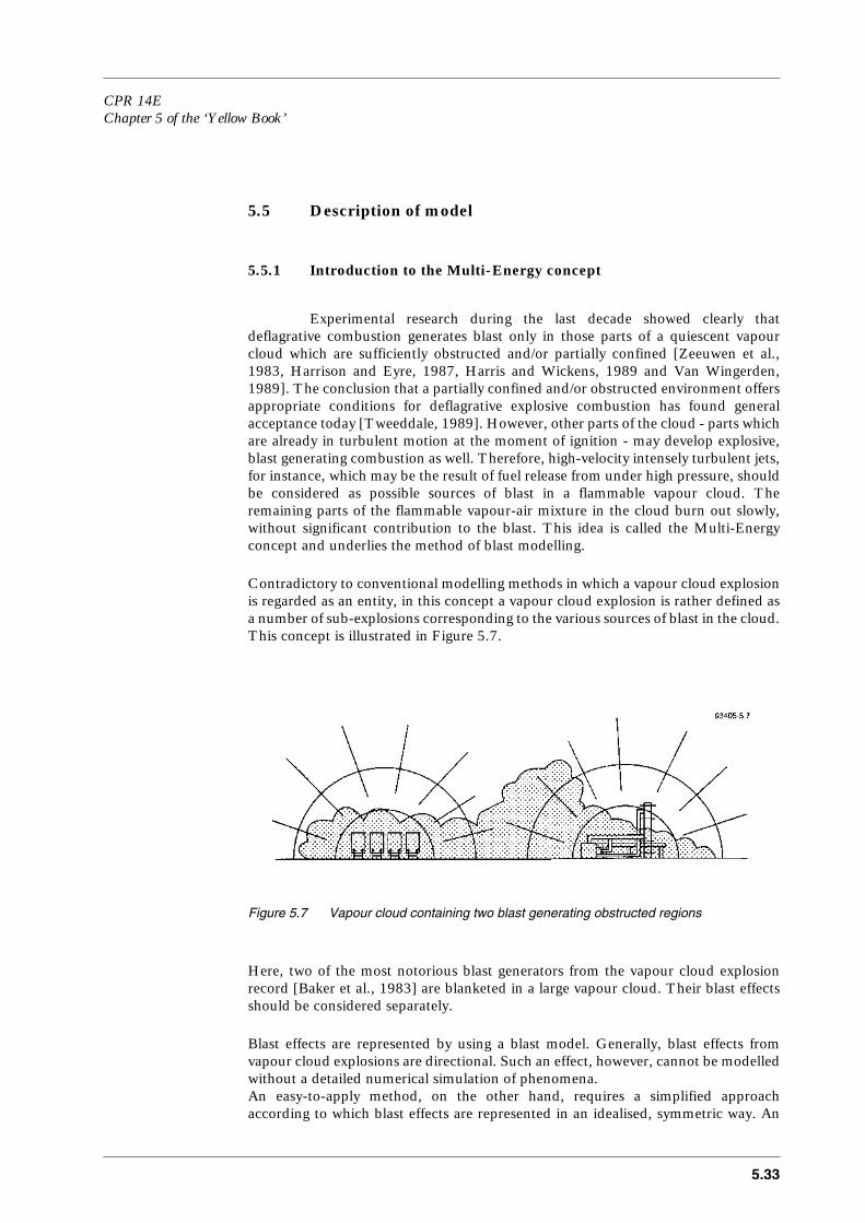
CPR 14EChapter 5 of the ‘Yellow Book’
5.33
5.5 Description of model
5.5.1 Introduction to the Multi-Energy concept
Experimental research during the last decade showed clearly thatdeflagrative combustion generates blast only in those parts of a quiescent vapourcloud which are sufficiently obstructed and/or partially confined [Zeeuwen et al.,1983, Harrison and Eyre, 1987, Harris and Wickens, 1989 and Van Wingerden,1989]. The conclusion that a partially confined and/or obstructed environment offersappropriate conditions for deflagrative explosive combustion has found generalacceptance today [Tweeddale, 1989]. However, other parts of the cloud - parts whichare already in turbulent motion at the moment of ignition - may develop explosive,blast generating combustion as well. Therefore, high-velocity intensely turbulent jets,for instance, which may be the result of fuel release from under high pressure, shouldbe considered as possible sources of blast in a flammable vapour cloud. Theremaining parts of the flammable vapour-air mixture in the cloud burn out slowly,without significant contribution to the blast. This idea is called the Multi-Energyconcept and underlies the method of blast modelling.
Contradictory to conventional modelling methods in which a vapour cloud explosionis regarded as an entity, in this concept a vapour cloud explosion is rather defined asa number of sub-explosions corresponding to the various sources of blast in the cloud.This concept is illustrated in Figure 5.7.
Figure 5.7 Vapour cloud containing two blast generating obstructed regions
Here, two of the most notorious blast generators from the vapour cloud explosionrecord [Baker et al., 1983] are blanketed in a large vapour cloud. Their blast effectsshould be considered separately.
Blast effects are represented by using a blast model. Generally, blast effects fromvapour cloud explosions are directional. Such an effect, however, cannot be modelledwithout a detailed numerical simulation of phenomena. An easy-to-apply method, on the other hand, requires a simplified approachaccording to which blast effects are represented in an idealised, symmetric way. An
5.34
idealised gas explosion blast model was generated by computation and is representedin Figures 5.8 A, B and C. Steady flame speed gas explosions were numericallysimulated with the BLAST-code [Van den Berg, 1980] and their blast effects wereregistered.The blast charts were composed for vapour cloud explosions having a combustionenergy Ev of 3.5 MJ/m3 which is the combustion energy for most hydrocarbonmixtures at stoichiometric concentration with air.
Only the most significant blast-wave parameters such as the side-on peakoverpressure, peak dynamic pressure and positive phase duration of the blast-wave,are represented dependent on the distance to the blast centre for a hemi-sphericalfuel-air charge of radius ro on the earth’s surface. The data are reproduced in a fullynon-dimensional (Sach’s-scaled) representation so that the blast parameters can beread off in any consistent set of units.
The initial strength of the blast is indicated by a number ranging from 1, for very low,up to 10, for detonative strength. The initial blast strength is defined as acorresponding set of blast-wave parameters at the location of the charge radius ro. Inaddition, a rough indication for the shape of the blast-wave is given. Detonative blastconsists of a shock-wave which is represented by solid lines. Pressure waves of lowinitial strength are indicated by dotted lines. Pressure waves may steepen to shock-waves in the far-field. In between, there is a state of transition indicated by dashedlines. The pictures show the characteristic behaviour of gas explosion blast. Pressurewaves, produced by a fuel-air charge of low strength, show an acoustic overpressuredecay behaviour and a constant duration in the positive phase. A much faster decayof the overpressure and a substantial increase of the positive phase duration isobserved for shock-waves in the vicinity of a charge of high initial strength.Eventually, the high-strength blast develops a more or less acoustic decay in the farfield.
Before the Multi-Energy method can be applied, the volume and the location of theflammable vapour cloud must be known or assumed. For this, source term modelsand dispersion models may be applied. Furthermore, the lay-out, or at least a roughimpression of the build-up area where the cloud is located, must be available in orderto determine the location, the number and the volume of the obstructed regionswithin the cloud. Then, the blast charts belonging to the Multi-Energy method canbe applied to obtain values for the most important blast parameters.

CPR 14EChapter 5 of the ‘Yellow Book’
5.35
Figure 5.8A Multi-Energy method blast chart: peak side-on overpressure

5.36
Figure 5.8B Multi-Energy method blast chart: peak dynamic pressure

CPR 14EChapter 5 of the ‘Yellow Book’
5.37
Figure 5.8C Multi-Energy method blast chart: positive phase duration and blast-wave shape
The blast parameters are read off the blast charts (Figures 5.8):
– calculate the scaled distance r’ which is the distance r of the location underconsideration to the centre of the explosion divided by the energy available E andthe ambient pressure pa:
r’ = r/(E/pa)1/3 (-) (5.2)
– assume an explosion strength (class 1 to 10) and read off the charts the scaled peakside-on overpressure Ps’, the scaled peak dynamic pressure pdyn’ and the scaledpositive phase duration tp’
– calculate the peak overpressure Ps from:
Ps = Ps’ × pa (Pa) (5.3)
5.38
– calculate the positive phase duration tp from:
tp = tp’ × (E/pa)1/3/aa (s) (5.4)
– calculate the peak dynamic pressure pdyn from:
pdyn = pdyn’ × pa (Pa) (5.5)
– determine the shape of the blast-wave from Figure 5.8C
– calculate the positive impulse is by integrating the overpressure variation duringthe positive phase resulting in multiplying the side-on overpressure with thepositive phase duration and with a factor 1/2:
is = 1/2 × Ps × tp (Pa⋅s) (5.6)
An interesting feature is that at a distance larger than about 10 charge radii from thecentre, the blast is independent on whether the explosion was a strong deflagration(higher than, or equal to, number 6) or a detonation (see Figure 5.8). Using thishemi-spherical fuel-air charge blast model, the blast produced by the various sourcesin the cloud can be modelled.
Contrary to more conventional methods, in the Multi-Energy concept the explosionhazard is not primarily determined by the fuel-air mixture itself, but above all by theenvironment in which the vapour disperses - the boundary conditions to thecombustion process. If somewhere a release of fuel is anticipated, the explosionhazard assessment can be limited to an investigation of the environment on potentialblast generative capabilities.
Today, it is recognised more and more that it is very unlikely to have a detonation ina fuel-air cloud originating from an accidental release in the open. The point is thatthe inhomogeneity of the fuel-air mixture in the cloud, which is inherent to theprocess of atmospheric turbulent dispersion, generally prevents a possible detonationfrom propagating [Van den Berg et al., 1987]. The heavy explosion on December 7,1970 at Port Hudson, MO., where almost all of a large unconfined vapour clouddetonated, should be blamed on an exceptional coincidence of circumstances.Lingering in a shallow valley under calm atmospheric conditions, a dense propane-aircloud had the opportunity to homogenise sufficiently by molecular diffusion duringan exceptionally long ignition delay [NTSB, 1972 and Burgess and Zabetakis, 1973].This incident is unprecedented, to our knowledge.Therefore, in a vast majority of cases the assumption of deflagrative combustion is asufficiently safe approach in a vapour cloud explosion hazard assessment.Deflagrative overpressures in a confined area, however, can lead to blast comparableto blast from a detonation.
CPR 14EChapter 5 of the ‘Yellow Book’
5.39
5.5.2 Discussion
Deficiencies of the model
The Multi-Energy method is expected to reasonably match reality, wearing the abilityto predict high, respectively low, overpressures in cases where they may be expected. Nevertheless, some deficiencies still exist and these should be covered before a solidprocedure for the application method is possible.These deficiencies concern:– the overpressure in an obstructed region (the ‘source strength’ or ‘class number’),– the definition of an obstructed region,– the minimal distances between potential explosion sources for which these sources
can be assumed to act independently (the ‘separation distance’).
Available guidance on the choice for the source strength
Since the introduction of the Multi-Energy method [Van den Berg, 1985], especiallythe lack of guidance in the choice of the source strength has been recognised and sincethen some guidance has become available. This is summarised next.
SRD, AEA Technology [Kinsella, 1993]
Kinsella [1993] provides guidance, based on a review of major accidents, to how toaccount, in the Multi-Energy method, for the influence of:– degree of obstruction by obstacles inside the vapour cloud,– ignition energy,– degree of confinement.
These three blast source strength factors are defined as follows.
– Obstruction:– High
Closely packed obstacles within gas cloud giving an overall volume blockagefraction (i.e. the ratio of the volume of the obstructed area occupied by theobstacles and the total volume of the obstructed area itself) in excess of 30%and with spacing between obstacles less than 3 m.
– LowObstacles in gas cloud but with overall blockage fraction less than 30% and/orspacing between obstacles larger than 3 m.
– NoneNo obstacles within gas cloud.
– Parallel plane confinement:– Yes
Gas clouds, or parts of it, are confined by walls/barriers on two or three sides.– No
Gas cloud is not confined, other than by the ground.
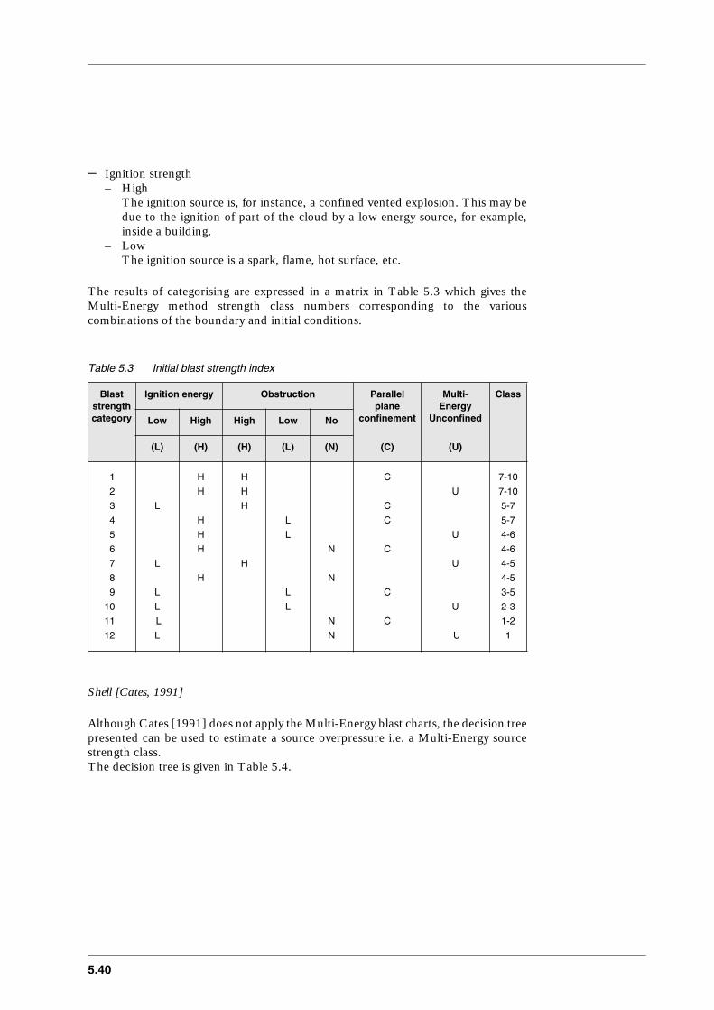
5.40
– Ignition strength– High
The ignition source is, for instance, a confined vented explosion. This may bedue to the ignition of part of the cloud by a low energy source, for example,inside a building.
– LowThe ignition source is a spark, flame, hot surface, etc.
The results of categorising are expressed in a matrix in Table 5.3 which gives theMulti-Energy method strength class numbers corresponding to the variouscombinations of the boundary and initial conditions.
Table 5.3 Initial blast strength index
Shell [Cates, 1991]
Although Cates [1991] does not apply the Multi-Energy blast charts, the decision treepresented can be used to estimate a source overpressure i.e. a Multi-Energy sourcestrength class.The decision tree is given in Table 5.4.
Blaststrengthcategory
Ignition energy Obstruction Parallel plane
confinement
(C)
Multi-Energy
Unconfined
(U)
Class
Low High High Low No
(L) (H) (H) (L) (N)
1 H H C 7-10
2 H H U 7-10
3 L H C 5-7
4 H L C 5-7
5 H L U 4-6
6 H N C 4-6
7 L H U 4-5
8 H N 4-5
9 L L C 3-5
10 L L U 2-3
11 L N C 1-2
12 L N U 1
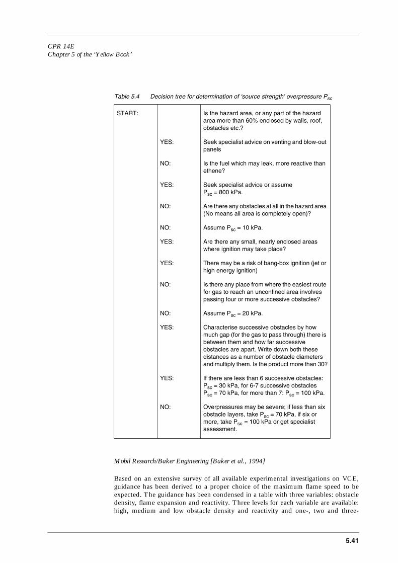
CPR 14EChapter 5 of the ‘Yellow Book’
5.41
Table 5.4 Decision tree for determination of ‘source strength’ overpressure Psc
Mobil Research/Baker Engineering [Baker et al., 1994]
Based on an extensive survey of all available experimental investigations on VCE,guidance has been derived to a proper choice of the maximum flame speed to beexpected. The guidance has been condensed in a table with three variables: obstacledensity, flame expansion and reactivity. Three levels for each variable are available:high, medium and low obstacle density and reactivity and one-, two and three-
START: Is the hazard area, or any part of the hazard area more than 60% enclosed by walls, roof, obstacles etc.?
YES: Seek specialist advice on venting and blow-out panels
NO: Is the fuel which may leak, more reactive than ethene?
YES: Seek specialist advice or assumePsc = 800 kPa.
NO: Are there any obstacles at all in the hazard area (No means all area is completely open)?
NO: Assume Psc = 10 kPa.
YES: Are there any small, nearly enclosed areas where ignition may take place?
YES: There may be a risk of bang-box ignition (jet or high energy ignition)
NO: Is there any place from where the easiest route for gas to reach an unconfined area involves passing four or more successive obstacles?
NO: Assume Psc = 20 kPa.
YES: Characterise successive obstacles by how much gap (for the gas to pass through) there is between them and how far successive obstacles are apart. Write down both these distances as a number of obstacle diameters and multiply them. Is the product more than 30?
YES: If there are less than 6 successive obstacles: Psc = 30 kPa, for 6-7 successive obstaclesPsc = 70 kPa, for more than 7: Psc = 100 kPa.
NO: Overpressures may be severe; if less than six obstacle layers, take Psc = 70 kPa, if six or more, take Psc = 100 kPa or get specialist assessment.
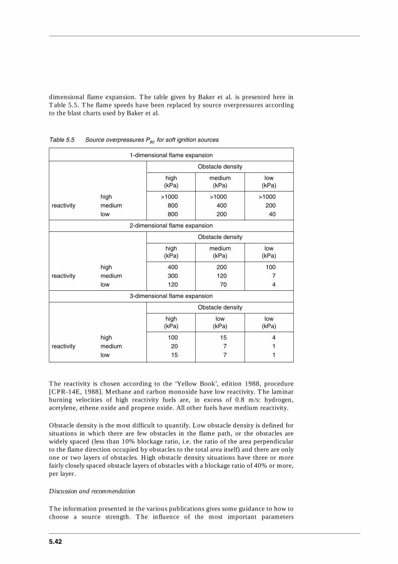
5.42
dimensional flame expansion. The table given by Baker et al. is presented here inTable 5.5. The flame speeds have been replaced by source overpressures accordingto the blast charts used by Baker et al.
Table 5.5 Source overpressures Psc for soft ignition sources
The reactivity is chosen according to the ‘Yellow Book’, edition 1988, procedure[CPR-14E, 1988]. Methane and carbon monoxide have low reactivity. The laminarburning velocities of high reactivity fuels are, in excess of 0.8 m/s: hydrogen,acetylene, ethene oxide and propene oxide. All other fuels have medium reactivity.
Obstacle density is the most difficult to quantify. Low obstacle density is defined forsituations in which there are few obstacles in the flame path, or the obstacles arewidely spaced (less than 10% blockage ratio, i.e. the ratio of the area perpendicularto the flame direction occupied by obstacles to the total area itself) and there are onlyone or two layers of obstacles. High obstacle density situations have three or morefairly closely spaced obstacle layers of obstacles with a blockage ratio of 40% or more,per layer.
Discussion and recommendation
The information presented in the various publications gives some guidance to how tochoose a source strength. The influence of the most important parameters
1-dimensional flame expansion
Obstacle density
high(kPa)
medium(kPa)
low(kPa)
high >1000 >1000 >1000reactivity medium 800 400 200
low 800 200 40
2-dimensional flame expansion
Obstacle density
high(kPa)
medium(kPa)
low(kPa)
high 400 200 100reactivity medium 300 120 7
low 120 70 4
3-dimensional flame expansion
Obstacle density
high(kPa)
low(kPa)
low(kPa)
high 100 15 4reactivity medium 20 7 1
low 15 7 1
CPR 14EChapter 5 of the ‘Yellow Book’
5.43
obstruction and confinement is shown. Kinsella [1993] takes into account theignition strength while Baker [1994], and to some extent Cates [1991], addsreactivity.Obstruction is characterised by either an obstacle volume blockage or an obstacle areablockage. Furthermore, the distance between obstacles for flame acceleration ismaximised. This guidance demonstrates the influence of the most importantparameters involved.
It should be emphasised though that application of this guidance is highlyquestionable. Still large uncertainties exist (as mentioned by the authors of thesearticles also) and absolute values for parameters should be distrusted. Results fromexperiments show that the actual overpressure can easily be underestimated by afactor 10 (or even up to a factor 30) when using this guidance [Mercx et. al., 1994].
It is therefore recommended to be conservative in the choice of a source strength forthe initial blast and not to use this guidance at all.
The problems to quantify the influence of obstruction do not exist for thequantification of the reactivity. Based on scaling laws it is possible to predict theinfluence on the explosion effect if the type of gas is changed [Mercx et. al., 1994]. Itis possible to obtain a relative rating with these laws. However, a reference is requiredfor an absolute quantification and for that the influence of obstruction should bequantified too. One could decide on the maximum overpressure of methane forinstance. British Gas assumes a maximum overpressure of four bars (4⋅105 Pa)[Harris and Wickens, 1989], (see 5.3.2). This value complies with an explosion classof almost nine. Starting with this reference excludes the possibility of reactivityclassification as most gases are more reactive than methane. This would lead toexplosion class nine and ten only.Therefore, the lack of knowledge of how to classify obstructions prohibits theclassification for reactivity.
As a result, a proper choice for the initial strength of the blast-wave from anobstructed region cannot be motivated presently. It is recommended:– to differentiate between obstructed and non-obstructed regions,– to choose a high initial blast strength for each obstructed region: number 10,– to choose a low initial blast strength for the remaining unobstructed region:
number 1. In case initial low turbulence motion is expected in non-obstructedregions, for instance, due to the momentum of the fuel release, a number of 3 isadvised,
– not to differentiate between reactivities.
If such a safe and conservative approach results in unacceptably high overpressures,a more accurate estimate for the initial blast strength may be found by consulting thegrowing body of experimental data on gas explosions, or by performing an experimenttailored to the situation in question.Another possibility is numerical simulation with advanced computational fluiddynamic codes such as FLACS [Hjertager, 1982 and 1989], PHOENIX [Kjäldmanand Huhtanen, 1985] or REAGAS [Van den Berg, 1989]. A way in which such codescould be utilised for vapour cloud explosion blast modelling has been demonstratedby Van den Berg et al. [1991]. The initial strength of the blast, however, is still a major issue of research.

5.44
It should be noted that applying the Multi-Energy method with an explosion classnumber 10, the overpressures will be similar to those obtained by applying the TNT-equivalence method with an efficiency factor of 20% to the obstructed part of thecloud (and not to the whole cloud).
5.5.3 Procedure for the division of an area into obstructed and unobstructed regions
A procedure to subdivide a region into obstructed and unobstructed partsis presented next.
The procedure given is thought to be safe and conservative in the sense that alwaystoo large a volume of the obstructed region will be selected. The procedure offers apossibility for optimisation, i.e. reduction, of the obstructed volume. Thisoptimisation procedure can be followed but obviously requires more time. Theoptimisation procedure in itself will not lead to unsafe situations.
The procedure to build-up an obstructed region is based on the effect obstacles haveon the generation of turbulence in the expansion flow ahead of the flame. A zone withobstacle induced turbulence will exist behind an obstacle. The length of this zone isrelated to a characteristic dimension of the obstacle. However, if the scale of anobstacle becomes larger, it is assumed that the length of the influenced zone isbounded by an upper value.
The procedure is as follows.
Step 1: break-down structures into basic geometrical structural shapes
Structures in a potential hazardous area like an industrial site may be considered asbeing composed of (or fairly well bounded by) basic geometrical shapes:– cylinders with length lc and diameter dc– boxes with dimensions b1, b2, b3– spheres with diameter ds
Step 2: assume an ignition location
After ignition of a flammable cloud in a congested area the flame will travel outwardso the orientation with respect to the flame propagation direction of each obstacle isknown.
Step 3: determine obstacle orientation
Take the smallest dimension oriented in a plane perpendicular to the flamepropagation direction to be D1, then:
D1 = lc or dc for a cylinderD1 = smallest of b1 and b2, b2 and b3, or b1 and b3 for a boxD1 = ds for a sphere
Take the obstacle dimension parallel to the flame propagation direction to be D2.

CPR 14EChapter 5 of the ‘Yellow Book’
5.45
Step 4: build-up of obstructed region
An obstacle belongs to an obstructed region if the distance from its centre to thecentre of any obstacle in the obstructed region is smaller than 10 times D1 or 1.5 timesD2 of the obstacle under consideration in the obstructed region (D1 and D2 belongingto any obstacle in the obstructed region).If the distance between the outer boundary of the obstructed region and the outerboundary of the obstacle is larger than 25 m, then the obstacle does not belong to thatobstructed region.
Note there are values given to three factors. These are a factor times D1 and a factortimes D2 (respectively 10 and 1.5) for obstacle distances, and a value (25 m) for thedistance between obstructed region and obstacle to determine if the obstacle is partof that obstructed region. It is not yet possible to quantify these values accurately. Thevalues given are thought to be safe though.
Step 5: defining a box containing the obstructed region
The obstructed region is defined as a box that contains all the obstacles in theobstructed region,including: the space between a confining surface and an obstructed region in case
the distance between that surface and any obstacle in the obstructedregion is less than 10 times D1 or 1.5 times D2 (for instance the earth’ssurface)
excluding: parts of cylinders or boxes that clearly do not belong to the obstructedregion, such as upper parts of chimneys, distillation columns (verticallyoriented cylinders) or pipes (horizontally oriented cylinders) connecting,for instance, chemical units, each potentially being an obstructed region,at a chemical plant.The excluded parts may form an obstructed region in themselves.
The free volume of the obstructed region Vr is de volume of the box minus the spaceoccupied by the obstacles. In case it is not possible to calculate or estimate the volumeoccupied by the obstacles, assume Vr equals the total volume of the box.
Step 6: subdivision into multiple boxes
The box containing the obstructed region smooths the outer boundary of the actualobstacle boundaries, thereby including additional space free of obstacles. In case thisfree space is not included in the obstructed region by the procedure for building-upthe obstructed region but by drawing the box around the obstructed region, sub-division into multiple directly adjacent boxes is acceptable for reducing the volume ofthe obstructed region.
Step 7: define additional obstructed regions if appropriate
In case not all obstacles present are inside the obstructed region, possibly moreobstructed regions within the cloud can be defined.In that case, the region where ignition occurs is called the ‘donor’ region, the otherregions are ‘acceptor’ regions.

5.46
The direction of flame propagation, required for the orientation of the obstacles in theacceptor region, depends on the orientation of the acceptor region with respect to thedonor region.
If separate obstructed regions are located close to each other, they may be initiatedmore or less at the same time. The coincidence of their blasts in the far-field may notbe ruled out and the respective blasts should be superposed.Presently there is no guidance to the minimum distance between donor and acceptorregions at which they can be assumed to be separate explosions. Due to this lack, agreat possibility of reducing the hazards of a vapour cloud explosion can not berealised. The procedure for applying the Multi-Energy method described in the nextsection contains a safe and conservative approach to cover this deficiency.
Remarks
Due to the choice of having a high initial blast strength for an obstructed region, theneed for having a clear definition of an obstructed region grows.The exact boundaries of an obstructed region are in fact not very important to thedetermination of blast. According to the blast charts (Figure 5.8), the energy E has tobe raised to the power of 1/3.
The subdivision of a hazardous site into obstructed and unobstructed regions and theattribution of a source strength to each region is a major issue in ongoing research. Asa simplified Multi-Energy method is applied here, a simplified procedure for thesubdivision into obstructed and unobstructed regions is adapted.
In order to obtain a rather straightforward, easy to apply and fully closed procedure,a number of influences which lead to reduction of the explosion severity, have beenneglected. This indicates that further optimisation is possible but that this should beobtained through consultation of experts.
5.5.4 Procedure for the application of the Multi-Energy method
The procedure of vapour cloud explosion blast modelling according to theMulti-Energy concept can be subdivided into a number of steps. Figure 5.9 showsthese successive steps.
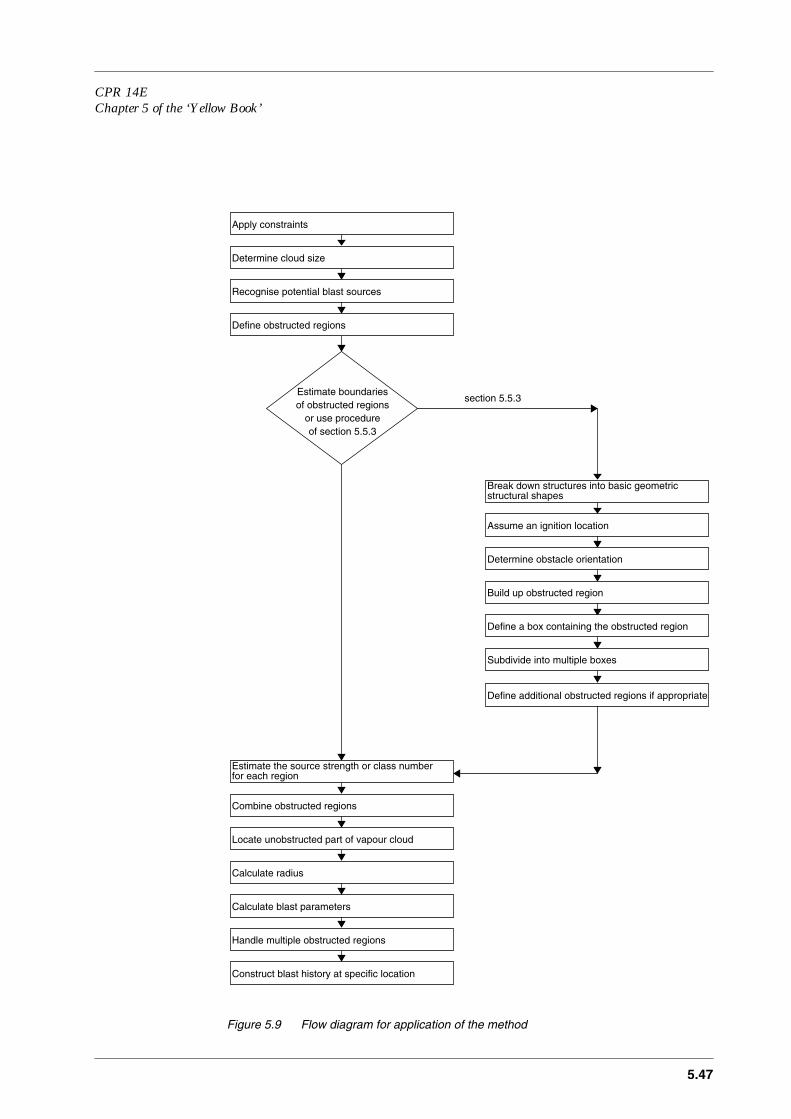
CPR 14EChapter 5 of the ‘Yellow Book’
5.47
Figure 5.9 Flow diagram for application of the method
Apply constraints
Determine cloud size
Recognise potential blast sources
Define obstructed regions
Break down structures into basic geometric
Assume an ignition location
Determine obstacle orientation
Build up obstructed region
Define a box containing the obstructed region
Subdivide into multiple boxes
Define additional obstructed regions if appropriate
Estimate the source strength or class number
Combine obstructed regions
Locate unobstructed part of vapour cloud
Calculate radius
Calculate blast parameters
Handle multiple obstructed regions
Construct blast history at specific location
for each region
structural shapes
Estimate boundaries
or use procedureof obstructed regions
of section 5.5.3
section 5.5.3
5.48
Step 1: application constraints
– Realise that the Multi-Energy method is used for determination of the blastparameters from ‘unconfined’ vapour cloud explosions. Blast from vented vapourcloud explosions and from internal explosions should be assessed using othermethods. These methods can be either semi-emperical like the methods of Bradleyand Mitcheson [Harris, 1983] or deterministic like the computational fluiddynamics (CFD) codes AutoReaGas, FLACS, EXSIM and others.
– Realise that the Multi-Energy method is a simplification of reality. It does not takeinto account directional blast effects due to the inhomogeneous distribution ofconfinement and obstruction of the vapour cloud or due to the non-point-symmetrical shape of the vapour cloud. Use more sophisticated models, like theCFD codes mentioned above, to assess these aspects.
– Assume that blast modelling on the basis of deflagrative combustion is asufficiently safe and conservative approach. Keep in mind that unconfined vapourcloud detonation is extremely unlikely and has only a single precedent, to ourpresent knowledge.
Step 2: determination of cloud size
– Determine the mass quantity after an accidental release that can contribute to theformation of a flammable cloud.
In general, a dispersion calculation will preceed the explosion calculation. Seesection 5.7 on how to calculate the flammable mass quantity within a cloud.In case no dispersion calculation is made, the mass quantity has to be estimated. In asafe approach one could assume that the whole mass inventory contained within theprocess unit under consideration, contributes to the formation of a flammable cloud.In case of pool evaporation one could multiply the evaporation rate by a certain timeperiod to come up with a mass quantity.
– Calculate the volume Vc of a cloud with a density ρ containing the flammable massquantity Qex at stoichiometric concentration cs (cs in vol.%) with:
Vc = Qex/(ρ × cs) (m3) (5.7)
Step 3: recognition of potential blast sources
– Identify potential sources of blast in the vicinity of a postulated location of thecentre of the cloud.
Potential sources of strong blast are, for example:– extended spatial configuration of objects, e.g. process equipment at chemical
plants or refineries piles of crates,– the space between extended parallel planes, e.g.
– underneath groups of closely parked cars on parking lots or marshalling yards,– open buildings, e.g. multi-story parking garages,
– the space in tubelike structures, e.g.– tunnels, bridges, corridors,– sewage systems, culverts,
– an intensely turbulent fuel-air mixture in a jet due to release at high pressure.

CPR 14EChapter 5 of the ‘Yellow Book’
5.49
Step 4: define obstructed regions
– Define obstructed regions using the procedure given in the previous section orestimate boundaries of obstructed regions and determine the free volume Vr ofeach obstructed region.
– Determine the maximum part of the cloud Vgr that can be inside the obstructedregions.
– Calculate the volume Vo of the unobstructed part of the vapour cloud with:
Vo = Vc - Vgr (m3) (5.8)
– Calculate the energy E of each region, obstructed as well as unobstructed, bymultiplying Vgr and Vo by the combustion energy per unit volume.
Step 5: estimate the source strength or class number for each region
As has been explained before, a conservative approach would be to choose a classnumber of 10 for each obstructed region. Other numbers may be chosen based onadditionally obtained information if required. Choose a low initial blast strength forthe remaining unobstructed regions: number 1. In case initial low turbulence motionis expected in unobstructed regions, for instance, due to the momentum of the fuelrelease, a number of 3 is advised.
Step 6: combination of obstructed regions
In case more than one obstructed region has to be considered:– Define an additional blast source (obstructed region) by adding all energies of the
separate blast sources together and by assuming a centre for the additional blastsource. This centre can be determined by considering the centres of the separateblast sources and their respective energies.
Step 7: location of unobstructed part of vapour cloud
– Determine a centre for the unobstructed vapour cloud volume. This centre can bedetermined by considering the centres of the separate unobstructed regions andtheir respective energies.
Now, a certain number of explosion centres and their respective energies E have beendetermined. For each centre the blast parameters as a function of distance to itscentre can be calculated using the blast charts given in Figure 5.8.
Step 8: calculate radius
– Model the blast from each source by the blast from an equivalent hemi-sphericalfuel-air charge of volume E/Ev m
3 (Ev = 3.5 MJ/m3 is an average value for mosthydrocarbons at stoichiometric concentration). Form an impression of the scaleby calculation the radius ro for each blast source from:
ro = (3/2 × E/(Ev × π))1/3 (m) (5.9)
5.50
Step 9: calculate blast parameters
The blast parameters at a specific distance r from a blast source can be read off Figure5.8 A, B and C after calculating the scaled distance r’.
– Calculate the scaled distance r’ with:
r’ = r/(E/pa)1/3 (-) (5.2)
– Depending on the class number 1, 3 or 10, read the scaled peak side-onoverpressure Ps’, the scaled dynamic peak pressure pdyn’ and the scaled positivephase duration tp’ off the respective blast charts in Figure 5.8.
– Calculate the peak side-on overpressure Ps, the peak dynamic pressure pdyn andthe positive phase duration tp with:
Ps = Ps’ × pa (Pa) (5.3)
pdyn = pdyn’ × pa (Pa) (5.5)
tp = tp’ × (E/pa)1/3/aa (s) (5.4)
– Determine the shape of the blast-wave from the Figure 5.8.
– Calculate the positive impulse is by integrating the overpressure variation over thepositive phase which can be approximated by multiplying the side-on overpressurewith the positive phase duration and with a factor 1/2:
is = 1/2 × Ps × tp (Pa⋅s) (5.6)
Step 10: handling of multiple obstructed regions
If separate blast sources are located close to each other, they may be initiated more orless at the same time. The coincidence of their blasts in the far-field may not be ruledout and the respective blasts should be superposed. This should be accomplished bytaking the respective quantities of combustion energy of the sources in questiontogether. To determine the parameters in the blast-wave at a specific distance, one should usethe blast source as defined in step 6.
Step 11: construct the blast history at a specific location
Combustion in the unobstructed region is considerably different from combustion inan obstructed region. Blast from an obstructed region will result in sharp andrelatively short peaks (shock-waves). The relatively slow combustion in anunobstructed region will result in pressure waves of long duration. Due to theinfluence of the respective energies, however, either of the blast-waves can be ofimportance at a specific location.

CPR 14EChapter 5 of the ‘Yellow Book’
5.51
It may be assumed that the blast history at a specific location consists of the blastparameters and blast shape resulting from the obstructed region on which the blastparameters of the unobstructed region are superposed.

5.52

CPR 14EChapter 5 of the ‘Yellow Book’
5.53
5.6 Application of selected models: calculation examples
5.6.1 Introduction to section 5.6
Examples are given to show how the procedures described in this chapterwork.In section 5.6.2 the procedure of defining and refining of an obstructed region iselucidated for a specific hazardous site.In section 5.6.3 ignition of a specific vapour cloud located in the hazardous site ofsection 5.6.2 is postulated and the blast parameters are determined. Two situations are considered in section 5.6.3. One in which the obstructed region islarger and one in which the obstructed region is smaller than the vapour cloud volume(respectively 5.6.3.1 and 5.6.3.2).Section 5.6.4 gives the determination of the obstructed region for a more complexlay-out.
5.6.2 Definition of an obstructed region
The boundaries of obstructed regions can be chosen by carefullyconsidering the lay-out of a hazardous site. In case of doubt or in case a more precisedefinition is required, the more time consuming procedure of section 5.5.3 can befollowed. This procedure will be followed here.
As an example for the build-up of obstructed regions on a hazardous site, an LPGstorage and distribution centre is chosen. The picture in Figure 5.10 shows anoverview. Figure 5.11 gives a map from which it becomes clear that the LPGinstallation at San Juan Ixhuatepec near Mexico City was the basis for this example[Pietersen, 1985].
The facility comprises 6 spherical storage tanks, 4 with a volume of 1600 m3 and 2with a volume of 2400 m3. An additional 48 horizontal cylindrical bullet tanks aresituated near the large spheres.The total storage capacity of about 16000 m3.The storage is subdivided into 6 zones, see Figure 5.12.Horizontal distances are given in Figure 5.13.
Additional dimensions are:– the minimum height underneath the bullet tanks is 2 m;– the minimum height underneath the spheres is 2 m;– additional pipework on top of cylinders and spheres has a height of 0.5 m;– the storage area is surrounded by an open corridor of 30 m width;– alongside the length of the outer cylinders, stairs with a width of 1.5 m are
situated.

5.54
Figure 5.10 Picture of LPG storage facility
From the first glance it will be clear that any of the groups of cylinders or spheres arean obstructed region.
Step 1: break-down of structures into basic geometrical structural shapes
The structures exist of big spheres and cylinders. Other structures like stairs,walkways, supports, pipes will not be considered here. This is a valid approach: thedimensions of the large obstacles will dominate the process of building an obstructedregion: 10 times D1 of a big obstacle will override 10 times D1 of a small obstaclelocated near the larger one (step 4). Figure 5.12 shows all major basic geometricalstructural shapes.
Step 2: assume an ignition location
Assume ignition in the centre of the southern group of cylinders in zone 4(figure 5.13).
The build-up of the obstructed region is started by taking the cylinder west of theignition location as a start (marked as 1).
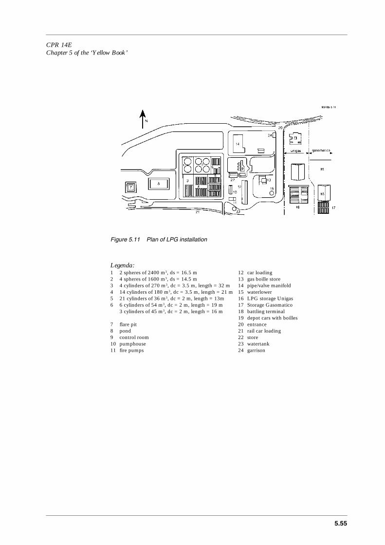
CPR 14EChapter 5 of the ‘Yellow Book’
5.55
Figure 5.11 Plan of LPG installation
Legenda:1 2 spheres of 2400 m3, ds = 16.5 m 12 car loading2 4 spheres of 1600 m3, ds = 14.5 m 13 gas boille store3 4 cylinders of 270 m3, dc = 3.5 m, length = 32 m 14 pipe/valve manifold4 14 cylinders of 180 m3, dc = 3.5 m, length = 21 m 15 waterlower5 21 cylinders of 36 m3, dc = 2 m, length = 13m 16 LPG storage Unigas6 6 cylinders of 54 m3, dc = 2 m, length = 19 m 17 Storage Gasomatico
3 cylinders of 45 m3, dc = 2 m, length = 16 m 18 battling terminal19 depot cars with boilles
7 flare pit 20 entrance8 pond 21 rail car loading9 control room 22 store10 pumphouse 23 watertank11 fire pumps 24 garrison
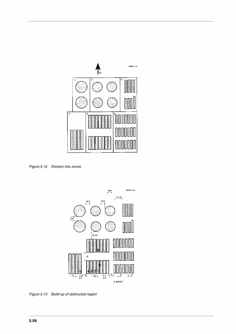
5.56
Figure 5.12 Division into zones
Figure 5.13 Build-up of obstructed region
CPR 14EChapter 5 of the ‘Yellow Book’
5.57
Step 3: determine obstacle orientation
In order to decide whether cylinder 2 is part of the obstructed region, values for D1and D2 have to be determined. Following the direction of flame propagation from theignition location, via cylinder 1 towards cylinder 2, the orientation of the axis ofcylinder 1 is perpendicular to the direction of flame propagation. Therefore both D1and D2 equal the diameter 3.5 m in this case.
Step 4: build-up of obstructed region
The distance between cylinder 1 and the adjacent, cylinder 2 is 1.5 m. This distanceis smaller than 10 times D1 and also smaller than 1.5 times D2. Thus, cylinder 2 ispart of the obstructed region.
The obstructed region is enlarged to include now cylinder 1 and 2.
It is obvious that all seven cylinders of the southern group in zone 4 are within oneobstructed region.
The distance between the east cylinder in zone 3 (number 5) and the west cylinder ofthe obstructed region (number 4) is 11.5 m. D1 and D2 both equal still 3.5 m. Thuscylinder 5 belongs to the obstructed region too.It is can be easily derived that all 4 cylinders of zone 3 belong to the obstructed regionalso.
The distance between the northern and southern group of cylinders in zone 4 is 13 m.In this case D1 = 3.5 m and D2 = 21 m. The distance of 13 m is smaller than 10 timesD1 and 1.5 times D2. Thus, cylinder 6 and all other cylinders in that group are partof the obstructed region.
Repeating the procedure for the other cylinder groups as well as the spheres, resultsin one obstructed region covering all cylinders and spheres. Additional pipework and stairs located within a distance of D1 or D2 from a sphere orcylinder belongs to the obstructed region too.
Step 5: define box containing the obstructed region
A box containing all obstacles in the obstructed region has the following dimensionslength: 108.5 m, width 110 m, and height 19.5 m (Figure 5.14, 19.5m is the heightof the highest cylinder including pipework on top).The space underneath the obstacles is part of the obstructed region too, the distanceof 2m to a confining surface (the earth) is smaller than 10 times D1 or 1.5 D2, or allbig obstacles.
A single big box in this case includes large volumes of free space, due to the largevariation in height between cylinders and spheres. A sub-division into multipledirectly adjacent boxes is therefore beneficial.
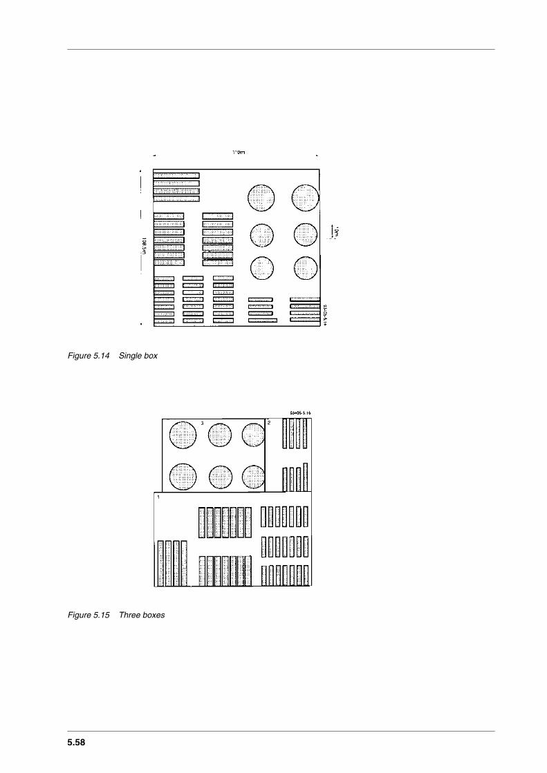
5.58
Figure 5.14 Single box
Figure 5.15 Three boxes
CPR 14EChapter 5 of the ‘Yellow Book’
5.59
Step 6: subdivision in multiple boxes
A first subdivision into 3 boxes is shown in Figure 5.15Box 1: contains the cylinders in zones 3,4 and 5;
dimensions: length 108.5 m, width 65 m and height 6 m.Box 2: contains the cylinders in zone 6;
dimensions: length 45 m, width 31.25 m and height 4.5 m.Box 3: contains all spheres in zone 1 and 2;
dimensions: length 65.5 m, width 45 m, height 19.5 m.
A second further subdivision is possible as the free space in box 1 north of zone 3 doesnot belong to the obstructed region. All other free space between groups of cylindersare part of the obstructed region and can therefore not be excluded by furthersubdivision into multiple boxes.
Figure 5.16 Four boxes
We now have four boxes (Figure 5.16):Box 1: contains the cylinders in zone 3 and the space between zones 3 and 4;
dimensions: length 32 m, width 31.5 m, height 6 m.Box 2: contains the cylinders in zones 4 and 5 and the space between zones 4 and
2, and 5 and 6;dimensions: length 77 m, width 65 m and height 6 m.
Box 3: contains the cylinders in zone 6;dimensions length 45 m, width 31.25 m and height 4.5 m.
Box 4: contains all spheres in zone 1 and 2;dimensions: length 65.5 m, width 45 m, height 19.5 m.

5.60
The volume of the obstructed region is the sum of the volumes of the four boxesminus the space occupied by the obstacles:Box 1: 32 × 31.5 × 6 = 6048 m3
Box 2: 77 × 65 × 6 = 30030 m3
Box 3: 45 × 31.25 × 4.5 = 6328 m3
Box 4: 65.5 × 45 × 19.5 = 57476 m3
Total volume = 99882 m3
The volume of the cloud inside the obstructed region is determined by deduction ofthe volume of the cylinders and spheres of the volume of the obstructed region.
The storage capacity is 16000 m3 which is assumed to equal the volume of the storagevessels.
So: Vgr = 99882 - 16000 = 83882 m3
Obviously, further subdivision is possible and acceptable as long as the rules forsubdivision are followed. One has to balance the benefit from further subdivision(which can be rather small) with the required time to perform the subdivision (whichcan be rather long) in order to decide to which level of detail subdivision is carriedout.
Step 7: define additional obstructed regions if appropriate
As all obstacles present are inside the one obstructed region defined, no additionalobstructed regions are requested.
5.6.3 Vapour cloud explosion
Vapour cloud smaller than obstructed region
The blast parameters resulting from a vapour cloud explosion located in the LPGstorage facility of the example in section 5.6.2 will be determined. A table will becomposed showing at what distances a specific side-on overpressure is expected tooccur. The other blast parameters are calculated at these distances.
Step 1: application constraints
The incident of an accidental release of flammable material will probably have anumber of effects with a number of consequences. Due to the explosion, dominoeffects are expected. Pressurised vessels may be shifted and damage and even fail,creating physical explosions, BLEVES, fires and missiles.The Multi-Energy method is to be used for the determination of the blast parametersas a result of a relatively large and initially non-turbulent flammable fuel-air cloud.Determination of blast as a result of bursting vessels is treated in chapter 7 ‘Ruptureof Vessels’.

CPR 14EChapter 5 of the ‘Yellow Book’
5.61
Step 2: determination of cloud size
Due to a failure of a feed pipe to one of the cylindrical vessels, a certain amount ofliquid propane is spilt in the bunt underneath the vessels. The spill starts to evaporateand a fuel-air cloud is generated which fills the space between the storage tanks. It isassumed that at the moment of ignition 4750 kg liquid propane has evaporated.
It is assumed that the evaporated propane has mixed with air stoichiometrically (4%)and that the temperature of the mixture is 15 ˚C.The density of propane vapour at 15 ˚C is 1.86 kg/m3 so the volume of the cloudequals
Vc = 100/4 × 4750/1.86 = 63844 m3
Step 3: recognition of potential blast sources
Here, only blast sources relating to a vapour cloud explosion are at issue.According to the guidance given in section 5.5.4, potential blast sources areunderneath all cylinders and spheres.
Step 4: define obstructed regions
The example in section 5.6.2 defines a single obstructed region comprising fourboxes. It is calculated there that
Vgr = 83882 m3
The volume of the vapour that can be contained in the obstructed region is larger thanthe volume of the assumed cloud. Therefore Vgr is reduced to Vc:
Vgr = Vc = 63844 m3
The centre of the vapour cloud is taken as the approximate centre of the obstructedregion: the north end of the most eastern cylinder in the northern cylinder group ofzone 4 see Figure 5.16.
The volume of the unobstructed part of the cloud is zero:
Vo = 0 m3
The heat of combustion of a stoichiometric propane air mixture is 3.46 MJ/m3 so theenergy E of the blast source is:
E = 3.46 × 106 × 63844 = 221 GJ
Step 5: estimate the source strength
A strength number 10 is selected.

5.62
Step 6: combination of obstructed regions
Not applicable.
Step 7: location of unobstructed part of the cloud
Not applicable.
Step 8: calculate radius
From equation (5.9):
follows: ro = 31 m
Step 9: calculate blast parameters
In case one wants to know at which distance a specific overpressure occurs (forinstance Ps = 10 kPa):
The dimensionless peak side-on overpressure is:
Ps’ = Ps/pa = 10/100 = 0.1
Select on the vertical axis of Figure 5.8C the value 0.1 and pick the point where thepressure decay line belonging to a class strength of 10 crosses this value. Select on thehorizontal axis the value of the scaled distance that belongs to the scaled pressure of0.1 and the class 10 line.
It is found that:
r’ = 3
The actual distance equals:
r = r’ × (E/pa)1/3 = 3 × (221 × 109/1 × 105)1/3 = 3 × 128 = 385 m
The other blast parameters at that distance are calculated as follows:
The positive phase duration tp at a distance of 390 m is:
r’ = 3
From Figure 5.8C:
tp’ = 0.38 (class 10)
tp = tp’ × (E/pa)1/3 /aa = 0.38 × (221 × 109/1 × 105)1/3 / 340 = 0.146 s = 146 ms
ro3
2 π×----------- 63844×
1/3
=
CPR 14EChapter 5 of the ‘Yellow Book’
5.63
The positive impulse:
is = 1/2 × Ps × tp = 1/2 × 104 × 0.146 = 730 Pa⋅s
The peak dynamic pressure, use figure 5.8B:
at r’ = 3:
pdyn’ = 0.003 (class 10)
pdyn = pdyn’ × pa = 0.003 × 1 × 105 = 300 Pa
The shape of the blast-wave:
The pressure decay line belonging to class 10 is solid, which means the shape of theblast is that of a shock-wave.
To get an impression of distances and blast parameters, Table 5.6 shows the result ofsome calculations.
Table 5.6 Distances for specific blast overpressures and remaining blast parameters
Vapour cloud larger than obstructed region
The hazardous location is now assumed to consists only of the cylindrical vessels ofzone 4 (Figure 5.12). All other data remains similar to that in section 5.6.2.
A table will be composed similar to Table 5.6 in order to get an impression of thereduction in distance at which a specific side-on overpressure is expected to occur.Also, the effect of the unobstructed part of the cloud is demonstrated.
Only the appropriate steps are addressed here:
Step 2:
Vc = 63844 m3
Ps r' r tp' tp pdyn is shape
(kPa) (-) (m) (-) (ms) (kPa) (Pa*s)
100 0.7 92 0.18 68 23 3403 shock-wave50 1 131 0.23 87 7.1 2184 shock-wave20 1.8 229 0.32 122 1.3 1210 shock-wave10 3 385 0.38 146 0.3 730 shock-wave5 5.2 682 0.44 168 < 0.01 419 shock-wave
5.64
Step 4:
The obstructed area is now a box enclosing all vessels, stairs and pipework in zone 4.The box has dimensions: length 37.5 m, width 55 m and height 6 m.
Vr = 37.5 × 55 × 6 = 12375 m3
Vgr = 37.5 × 55 × 6 - 14 × 180 = 9855 m3
Vgr < Vc
Vo = Vc - Vgr = 63844 - 9855 = 53989 m3
Obstructed region: E = 9855 × 3.46 × 106 = 34 GJ.Unobstructed region: E = 53989 × 3.46 × 106 = 187 GJ.
Step 5:
Class number for obstructed region is taken to be 10.Class number for unobstructed region is taken to be 3.
Step 7:
The location of the centre of both the obstructed and unobstructed region is taken tobe the centre of zone 4.
Step 8:
Obstructed region: ro = 16.8 m.Unobstructed region: ro = 29.5 m.
Step 9:
The blast parameters for the obstructed and unobstructed region are determined forspecific values of the peak side-on overpressure (Table 5.7A).For the distances r belonging to specific peak side-on overpressures, the blastparameters for the unobstructed region have been determined (Table 5.7B)

CPR 14EChapter 5 of the ‘Yellow Book’
5.65
Table 5.7A Distances for specific blast overpressures and remaining blast parameters (obstructed region, class 10)
Table 5.7B Distances for specific blast overpressures and remaining blast parameters (unobstructed region, class 3)
5.6.4 Determination of obstructed region
The lay-out of the previous example, the LPG storage and distributioncentre, was quit straightforward. Therefore, another example is given regardingdetermination of the obstructed region for a more complicated case.
Description of the site
Figure 5.17A shows a three-dimensional view of the chemical unit underconsideration. There only equipment is shown. Supporting structures and somebuildings were omitted for visuality. Figure 5.17B shows the floor plan at groundlevel. The unit is located on a rectangular site of 120 x 50 m.In order to get a better impression of the unit, additional Figures (5.17C through G)are added showing side-views from various locations. These locations are indicated inFigure 5.17A by C through G.The area is sub-divided into two small and two large sections by two perpendicularpipebridges (Figure 5.17H), both having a width of 8m, a height of 10m and lengthsof 100 and 50 m respectively. The main items within each sector are given next:
The two smaller sections consist of:– I: a storage area with the tanks AD16 and AD26, diameter 8m, height 12m.
total area 25 x 21 m2 (Figure 5.17 C);
Ps r' r tp' tp pdyn is shape
(kPa) (-) (m) (-) (ms) (kPa) (Pa*s)
100 0.7 50 0.18 37 22 1800 shock-wave50 1 70 0.23 47 7.2 1173 shock-wave20 1.7 122 0.32 65 1.3 653 shock-wave10 2.9 206 0.38 78 0.3 390 shock-wave5 5.2 365 0.44 90 < 0.01 225 shock-wave
Ps r' r tp' tp pdyn is shape
(kPa) (-) (m) (-) (ms) (kPa) (Pa*s)
5 0.58 72 2 734 0.73 1834 pressure wave4 0.81 100 2 734 0.3 1467 pressure wave3 1.1 136 2 734 0.12 1100 pressure wave2 1.7 204 2 734 < 0.1 733 pressure wave1 3.4 415 2 734 < 0.1 367 pressure wave
5.66
– II: substation #92, height 10m, total area 25 x 21 m2.
The two larger sections consist of vertical columns and installations on multi-levelsupporting structures: – III: columns AT3 diameter 5m, height 40m, with adjacent support structure
height 16m (Figure 5.17E);AT8 diameter 2.5m, height 12m (Figure 5.17E);AT4 diameter 5.8m, height 50m (Figure 5.17D);AD-433 diameter 4m, height 6m (Figure 5.17D);multi-level structure 25 x 15 m2 of variable height 16.5, 33 and 45m(Figure 5.17D);total area 87 x 21 m2;
– IV: columns AF1 average diameter 6m, height 40m (Figure 5.17G);AT5 diameter 5m, height 30m (Figure 5.17F);AT6 diameter 2.5m, height 15m (Figure 5.17F);multi-level structure 20 x 15 m2, with columns AR2A and AR2B diameter5m, height 20m (Figure 5.17F);total area 87 x 21 m2.
Determination of obstructed region
The flow diagram of section 5.5.4 gives the possibility to determine the volume of thecongested regions in two ways: by rough estimation or by the procedure of section5.5.3 in case such a procedure may be required.
Estimation of volume:
The average height of the site is assumed to be 15m. Together with outer dimensionsof 120 x 50 m, this leads to a volume of the obstructed region of 90000 m3.
Application of procedure:
Step 1: break-down structures into basic geometrical shapes
The installation consists of a combination of horizontally and vertically orientatedcylinders supported by elements such as beams and columns. There are some box-type shapes the largest of which is sub-station#92 in section I. The open multi-levelsupporting structures should be considered as composed of a number of smallergeometrical shapes, rather than one big shape. There are no spheres.The dimensions of the bigger obstacles are given next as it will appear (step 4) thatonly those are decisive for the build-up of the obstructed region:

CPR 14EChapter 5 of the ‘Yellow Book’
5.67
– Cylinder AD16, dc: 8 m, lc: 12 m;– Cylinder AD26, dc: 8 m, lc: 12 m;– Box #92, b1: 20 m, b2: 15 m, b3: 10 m;– Cylinder AT3, dc: 5 m, lc : 40 m;– Cylinder AT8, dc: 2.5 m, lc: 12 m;– Cylinder AT4, dc: 5.8 m, lc: 50 m;– Cylinder AF1, dc: 6 m, lc: 40 m;– Cylinder AD-433, dc: 4 m, lc: 6 m;– Cylinder AT5, dc: 5 m, lc: 30 m;– Cylinder AT6, dc: 2.5 m, lc: 15 m;– Cylinders AR-2A and B, dc: 4 m, lc: 20 m.
Step 2: assume ignition location
Ignition is assumed to occur in between the multi-level structure and AT3 in sectionIII. It is not expected that variation of the ignition location will result in variabledimensions of the congested region. The location has to be chosen for starting thebuild-up of the obstructed region in step 4.
Step 3: determine obstacle orientation
The flame will mainly propagate horizontally. Horizontal dimensions of the site arelarger than the vertical ones. The flame will pass more obstacles in the horizontalplane.For all vertical cylinders: D1 = dc and D2 = lc.
Step 4: build-up of obstructed region
The nearest large obstacle to the ignition location is AT3. It forms a congested regionwith all obstacles within a distance smaller than 10 x D1 or 25m. The latter value isdecisive in this case. This implies that the whole multi-level support structure insection III, the long pipebridge separating section III and IV, the multi-level supportstructure in sector IV and the area around AT8 is part of the obstructed region.
A big cylinder located in the multi-level structure in sector III is AD-433. Within10 x D1 (40m) or 25m of this cylinder, AT4 is located. So AT4 is also part of theobstructed region. Sector I and II as well as the shorter pipebridge are located within10 x D1 (58m) or 25m of AT4, so they are part of the obstructed region too.
AT6 is within 25m of AR-2B and AT5 is close to AT6, so these are included as wellas is AF1 which is located about 20m from AR-2A.
Some smaller horizontal oriented cylinders located along the long edges of the site(Figure 5.17A and B) are also within the obstructed region.
The procedure leads to the result that the whole site is part of the obstructed region.
The volume of the vapour cloud inside the obstructed region Vgr is to be determinedfrom the comparison of the free volume in the obstructed region Vr (step 5 fromparagraph 5.5.3) and the volume of a cloud with stoichiometric concentration Vc(step 2 of paragraph 5.5.4).

5.68
Step 5: defining a box containing the obstructed region
Step 6: subdivision into multiple boxes
A box containing the obstructed region has the dimensions of the site: 120 x 50m witha height equal to the highest vertical cylinder (50m, AT4).Subdivision into multiple boxes is done by reducing the height where possible, i.e.where the distance between obstacles is larger than 25m. A result is shown in Figure 5.17I. This figure shows the subdivision of the obstructedregion into multiple boxes. The height as well as the volume of each particular box isgiven. The boundary of the obstructed region is also indicated in Figures 5.17Cthrough G. Further subdivision is possible but will require considerable effort.
The total volume of the obstructed region equals 82421 m3.
Figure 5.17A Three-dimensional view of plant

CPR 14EChapter 5 of the ‘Yellow Book’
5.69
Figure 5.17B Horizontal cross-section
Figure 5.17C View from location C-C

5.70
Figure 5.17D View from location D-D

CPR 14EChapter 5 of the ‘Yellow Book’
5.71
Figure 5.17E View from location E-E

5.72
Figure 5.17F View from location F-F

CPR 14EChapter 5 of the ‘Yellow Book’
5.73
Figure 5.17G View from location G-G
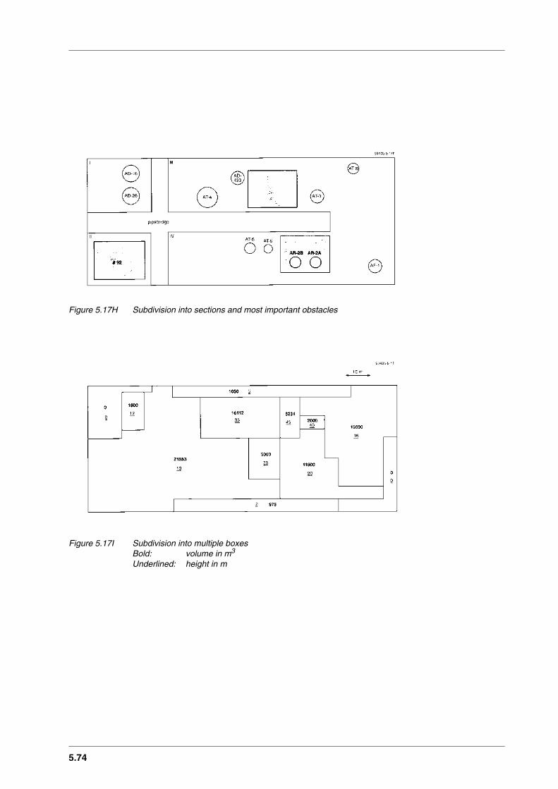
5.74
Figure 5.17H Subdivision into sections and most important obstacles
Figure 5.17I Subdivision into multiple boxesBold: volume in m3
Underlined: height in m
CPR 14EChapter 5 of the ‘Yellow Book’
5.75
5.7 Interfacing to other models
Input variables
The vapour cloud explosion blast model presented in this chapter describes thephysical effect of an explosion that may occur after ignition of a flammable vapourcloud. What is needed as input is:– the combustion energy involved in the explosion,– the location of the cloud at the moment of the explosion.
According to the Multi-Energy method, the combustion energy involved in theexplosion is the combustion energy of the confined fraction of the cloud. In order todetermine this fraction one has to determine the flammable mass quantity of thecloud.
Equations with which the flammable mass quantity of the cloud can be calculated aregiven in chapter 2 ‘Outfow and Spray Release’ and chapter 4 ‘Vapour clouddispersion’.
Entrainment with air is necessary to create a flammable cloud. Entrainment with airis calculated for:– a free jet (section 4.5.4.1),– a finite duration spray release (section 2.5.3.7),– an instantaneous release (section 2.5.3.8),– passive dispersion (section 4.5.3).
The flammable contents of the cloud created by the free jet is calculated usingequation (4.83).
The condition of the cloud for the finite duration spray release after flashing includingthe effects of rain-out are described by step 2 of the procedure given insection 2.5.3.7. Equation (2.164) provides a value for Af,rain-out. Af,rain-out togetherwith:
bf,rain-out = (Af,rain-out/π)1/2 (m) (5.10)
is the input for equations (4.81) and (4.82). The explosive content, including dropletsnot rained out, then follows from equation (4.83).
Instantaneous release is described in section 2.5.3.8. The concentration in the cloudis homogeneously distributed. The cloud is therefore flammable when thisconcentration is in between the lower and upper flammability limit. The explosivemass of the cloud can be calculated using equation (2.183).
Both the combustion energy involved and the cloud location can be determinedfollowing a dispersion calculation (chapter 4, section 4.5.3.7). Equation (4.65) of thatsection provides the mass of the flammable part of the cloud.

5.76
The flammable mass calculated using either of the above equations, is to bemultiplied by the combustion energy per unit volume. Table 5.1 gives this propertyfor some gases.
Output variables
The output of the model consists of the most important parameters to characterisethe blast-wave at a specific distance from the explosion centre for free field conditions.In order to gain knowledge about damage to structures and injury to people,additional models should be applied using the blast parameters as input. Models thatcan be used are described in CPR-16E [1990] chapters 2 and 3.
CPR 14EChapter 5 of the ‘Yellow Book’
5.77
5.8 Literature
Baker W.E., Cox P.A., Westine P.S., Kulesz J.J. and Strehlow R.A. (1983),Explosion hazards and evaluation,Fundamental studies in engineering, Vol.5, Elsevier Scientific Publishing Company, Amsterdam.
Baker Q.A., M.J. Tang and E Scheier (1994),Vapor cloud explosion analysis,AIChE 28th Loss Prevention Symposium, Atlanta, Georgia, USA, April 1994.
Brasie W.C. and Simpson D.W. (1968),Guidelines for estimating explosion damage,63rd National AIChE meeting, St Louis (MO), USA.
Brasie W.C. (1976),The hazard potential of chemicals,AIChE Loss Prevention, Vol.10, pp.135-140.
Burgess D.S. and Zabetakis M.G. (1973),Detonation of a flammable cloud following a propane pipeline break:the December 9, 1970, explosion in Port Hudson (MO),Bureau of Mines Report of Investigations No. 7752, United States Department of the Interior.
Cates A.T (1991),Fuel Gas explosion guidelines,Conference on fire and explosion hazards, Moreton-in-Marsh, April 1991.
CCPS (1994),Guidelines for evaluating the characteristics of vapor cloud explosions, flash fires and bleves, Center for Chemical Pocess Safety of the American Institute of Chemical Engineers.
CPR-14E (1988),Methods for the calculation of physical effects of the escape of dangerous materials,Ministry of Social Affairs and Employment, The Netherlands.
CPR-16E (1990),Methods for the calculation of possible damage to people and goods due to the physical effects of the escape of dangerous materials, Ministry of Social Affairs and Emplyoment, Voorburg, The Netherlands.
Desinov Yu. N., Shchelkin K.I. and TroshinYa.K. (1962),Some questions of analogy between combustion in a thrust chamber and a detonation wave,8th Int. Symp. on Combustion, Pittsburgh, PA, pp 1152-1159.

5.78
Eichler T.V. and Napadensky H.S. (1977),Accidental vapor phase explosions on transportation routes near nuclear power plants, IIT Research Institute final report no. J6405, Chicago (IL), USA.
Factory Mutual Research (1990),Private Communication.
French Authority Safety Rule (1982),Regle fondamentele de Surete I.2.d Prise en compte des risques lies a l’environnement industriel et aux voies de communication,Ministere de l’industrie, Paris.
French Chemical Industry (1986),Cahier de securite: Explosion de gaz en milieu confine,Union des Industries Chimiques.
Glasstone S. and Dolan P.J. Ed. (1977),The effects of nuclear weapons,US Dept.of Defence and US Dept.of Energy.
Gugan K. (1979),Unconfined vapour cloud explosions,The Institution of Chemical Engineers, UK.
Hanna S.R. and Drivas P.J. (1987),Guidelines for Use of Vapour Cloud Dispersion Models,AIChE, CCPS, New. York.
Harris R.J. (1983),The investigation and control of gas explosions in buildings and heating plant,E & F Spon Ltd, London, UK, 1983.
Harris R.J. and Wickens M.J. (1989),Understanding vapour cloud explosions - an experimental study,55th Autumn Meeting of the Institution of Gas Engineers, Kensington, UK.
Harrison A.J. and Eyre J.A. (1987),The effect of obstacle arrays on the combustion of large premixed gas/air clouds,Combustion Science and Technology, Vol.52, pp 121-137.
Hjertager B.H. (1982),Simulation of transient compressible turbulent flows, Combustion Science and Technology, Vol.27, pp 159-170.
Hjertager B.H. (1989),Simulation of gas explosions, Modeling, Identification and Control , Vol.10, No.4, pp 227-247.

CPR 14EChapter 5 of the ‘Yellow Book’
5.79
Health and Safety Executive (1979),Second Report Advisory Committee Major Hazards, U.K. Health and Safety Commission.
Health and Safety Executive (1986), The effect of explosions in the process industries,Loss Prevention Bulletin, No.68, pp 37-47.
Hopkinson B. (1915),British Ordnance Board Minutes 13565.
Industrial Risk Insurers (1990),Oil and Chemical Properties Loss Potential Estimation Guide,IRI-Information February 1.
IChemE (1994),Explosions in the Process Industries, Rugby, UK.
Jarrett D.E. (1968),Derivation of the British explosives safety distances, Anuals of the New York Academy of Sciences, Vol.152.
Kinsella K.G. (1993),A rapid assessment methodology for the prdiction of vapour cloud explosion overpressure, proceedings of the International Conference and Exhibition on Safety, Health and Loss Prevention in the Oil, Chemical and Process Industries, Singapore.
Kjäldman L. and R. Huhtanen (1985),Simulation of flame acceleration in unconfined vapour cloud explosions, Research report No 357, Technical Research Centre of Finland.
Lee J.H.S and Moen I.O. (1980),The mechanism of transition from deflagration to detonation in vapor cloud explosions, Prog. Energy Combustion Science, vol. 6 pp 359-389.
Luckritz R.T. (1977),An investigation of blast-waves generated by constant velocity flames, Aeronautical and Astronautical Engineering Department, University of Illinois, Urbana,Il ,USA, Technical report no. AAE 77-2.
Marshall V.C. (1976),The siting and construction of control buildings - a strategic approach, I.Chem.E.Symp.Series, No.47.
Mercx W.P.M., Johnson D.M. and Puttock J. (1994),Validation of scaling techniques for experimental vapour cloud explosion investigations, AIChE Loss Prevention Symposium, Atlanta, Georgia, USA, April 1994.

5.80
Munday G. (1976),Unconfined vapour-cloud explosions: A reappraisal of TNT equivalence, Inst. Chem. Eng. Symposium Series No.47, pp 19-38.
Nettleton M.A. (1987),Gaseous detonations, their nature, effects an control, Chapman and Hall, New York.
NTSB (1972),Pipeline Accident Report, Phillips Pipe Line Company propane gasexplosion, Franklin County (MO), December 9, 1970, National Transportation Safety Board, Washington (DC), report no. NTSB-PAR-72-1.
Pietersen C.M. and Cendejas Huerta S. (1985),Analysis of the LPG incident in San Juan Ixhuatepec, Mexico City, 19 November 1984, TNO report ref. 85-0222, May 1985, The Netherlands.
Robinson C.S. (1944),Explosions, their anatomy and destructiveness, McGraw-Hill, New York.
Sachs R.G. (1944),The dependence of blast on ambient pressure and temperature, BRL report No. 466, Aberdeen Proving Ground, Maryland, USA.
Schardin H. (1954),Ziviler Luftschutz, No.12, pp 291-293.
Strehlow R.A., Luckritz R.T., Adamczyk A.A. and Shimpi S.A. (1979),The blast-wave generated by spherical flames, Combustion and Flame, Vol.35, pp 297-310.
Tweeddale M. (1989),Conference report on the 6th Int.Symp. on Loss Prevention and Safety Promotion in the Process Industries, Journal of Loss Prevention in the Process Industries, Vol.2, No.4, pp 241.
Urtiew P.A. and Oppenheim A.K. (1966),Experimental observations of the transition to detonation in an explosive gas, Proceedings Royal Society London, A295:13-28.
Van den Berg A.C. (1980),BLAST - a 1-D variable flame speed blast simulation code using a ‘Flux-Corrected Transport’ algorithm, Prins Maurits Laboratory TNO report no.PML 1980-162, The Netherlands.

CPR 14EChapter 5 of the ‘Yellow Book’
5.81
Van den Berg A.C. (1985),The Multi-Energy method - A framework for vapour cloud explosion blastprediction, Journal of Hazardous Materials, Vol.12, pp 1-10.
Van den Berg A.C., Van Wingerden C.J.M., Zeeuwen J.P. and Pasman H.J. (1987),Current research at TNO on vapor cloud explosion modeling, Int.Conf.on Vapor Cloud Modeling, Cambridge (MA), USA, pp 687-711, AIChE, New York.
Van den Berg A.C. (1989),REAGAS - a code for numerical simulation of 2-D reactive gas dynamics in gas explosions, TNO Prins Maurits Laboratory report no. PML1989-IN48, The Netherlands.
Van den Berg A.C., Van Wingerden C.J.M. and The H.G. (1991),Vapor cloud explosion blast modeling, International Conference and Workshop on Modeling and Mitigation the Consequences of Accidental Releases of Hazardous materials, May 21-24, New Orleans, USA.
Van den Berg A.C. and A. Lannoy (1993),Methods for vapour cloud explosion blast modelling, Journal of Hazardous Materials, Vol 34, pp 151-171.
Van Wingerden C.J.M. (1989),Experimental investigation into the strength of blast-waves generated by vapour cloud explosions in congested areas, 6th Int. Symp. on Loss Prevention and Safety Promotion in the Process Industries, Oslo, Norway, pp 26-1,26-16.
Wiekema B.J. (1980),Vapour cloud explosion model, Journal of Hazardus Materials, Vol.3, pp 221-232.
Zeeuwen J.P. Van Wingerden C.J.M. and Dauwe R.M. (1983),Experimental investigation into the blast effect produced by unconfined vapour cloud explosions,4th Int. Symp. on Loss Prevention and Safety Promotion in the Process Industries, Harrogate, UK, ChemE Symp.Series No.80, pp D20-D29.

6.1
Chapter 6Heat flux from firesW.F.J.M. Engelhard

CPR 14EChapter 6 of the ‘Yellow Book’
6.3
Modifications to Chapter 6 (Heat Flux from Fires)with respect to the first print (1997)
Numerous modifications were made concerning typographical errors. A list is givenbelow for the pages on which errors have been corrected.
Page 6.19: Corrected the sentence that in the appendix formulae a given tocalculate the view factor for all types of fires.
Page 6.29: Corrected the sentence above equation 6.5. The equations 6.5and 6.6 have been extended for readability in a more scientificway.
Page 6.33: Corrected the symbol a’, b’, c’ and d’ in the text.Page 6.34: Updated the symbols below equation 6.14. Corrected the last
sentence on the page wrt. the reference to the equations.Page 6.38: Updated the explanation of the symbols below equation 6.21.Page 6.47: Updated the equations 6.25 and 6.26.Page 6.53: Equation 6.35 for Mj for choked flow has been written down in
a more scientific way. The equation for Mj in case of unchokedflow has been added and also an explanation of the used symbolsin these equations.
Page 6.55: Included a note wrt. the constant 2.85 in the value for Cc. Theequation 6.44 has been updated and also the explanation of thesymbol Θjv.
Page 6.56: Updated equation 6.46 and 6.47 and the explanation of thesymbols below equation 6.47.
Page 6.57: Inserted the correct formulae for the calculation of the lift-off ofthe flame (b) in equation 6.49. Added below equation 6.49 theequation to calculate the value of (K) in equation 6.49.Corrected the equation 6.54
Page 6.65: Included a list of symbol explanations below equation 6.67.Noted below equation 6.13 that according to Mudan [84] u*<1
u*=1. In equation 6.12 the scaled wind velocity should beraised to the power of –0.21.
Page 6.87: In table 6.11, the values for LNG on water and land wereinterchanged.
Page 6.97 – 6.121: The calculation examples have been fully corrected foraccording to the above changes.
Appendix 6.1-7: Equation 6.14 has been updated for the typographical error !Appendix 6.1-9: The Figure 6.A.7 is for an elevated flame wrt. the target.Appendix 6.1-11: Below equation 6.A.30 an equation for B has been inserted.Appendix 6.1-12: The numerical values in Table 6.A.2 have been corrected and
updated. Appendix 6.1-13: Figure 6.A.11 has been updated wrt the values in Table 6.A.2.

6.4
CPR 14EChapter 6 of the ‘Yellow Book’
6.5
List of symbols Chapter 6
a Acceleration (6.76) m/s2
a Constant in Appendix (6.A.15) -a' Constant (6.16) -A Surface area of the flame (6.2) m2
A Constant in Appendix (6.A.8) -A0 Surface area of the leak (6.76) m2
Ap Surface area of the pool (6.7) m2
At Cross-sectional area of the tank (6.76) m2
dA1 Infinitesimal surface area (6.A.13) m2
dA2 Infinitesimal surface area (6.A.13) m2
b Frustum lift-off height (6.49) mb Constant in Appendix (6.A.15) -b In Appendix, the width of a flat radiator (6.A.28) mb' Constant (6.16) -B Constant in Appendix (6.A.9) -Bc ‘Spalding’ convection mass transfer number (6.88)c Variable tanΘ/cosΘ (6.70) -c' Constant (6.16) -c1 Constant (6.6) (m1.22⋅s0.61)/kg0.61
c2 Constant (6.10) sc3 Constant (6.19) J/(m2⋅s)c4 Constant (6.19) J/(m2⋅s)c5 Constant (6.19) m-1
c6 Constant (6.21) (N/m2)-0.32
c7 Constant (6.29) (N/m2)0.09⋅m0.09
c8 Constant (6.67) kg/(m2⋅s)c9 Constant (6.90) m/kg0.325
c10 Constant (6.91) s/kg0.26
C Constant in Appendix (6.A.15) -C' Factor (6.53) -Ca Constant (6.42) -Cb Constant (6.42) -Cc Constant (6.42) -Cp Specific heat capacity at constant pressure (6.9) J/(kg⋅K)Cv Specific heat capacity at constant volume (6.32) J/(kg⋅K)C0 Flow coefficient for fluids through a circular -
hole (6.75)d' Constant (6.17) -dh Diameter of the hole of the release point (6.83) mdj Diameter of the jet at the exit hole (6.41) mD Pool diameter (6.6) mD Constant in Appendix (6.A.15) -D' Actual elongated flame base diameter (6.18) mDmax Maximum diameter of pool fire (6.78) mDs Effective hole diameter (6.39) mDw The maximum pool dimension in the direction
of the wind (6.18) me' Constant (6.17) -E Constant in Appendix (6.A.15) -

6.6
f Fraction of the volume of the pressure tank, filledwith the flammable liquefied pressurised gas (6.89) -
f' Constant (6.17) -F Constant in Appendix (6.A.15) -Fh Geometrical view factor for the horizontal plane
of the radiated object (6.A.18) -Fmax Maximum geometrical view factor of the radiated
object (6.A.18) -Fs Fraction of the generated heat radiated from the flame
surface (6.3) -Fv Geometrical view factor for the vertical plane of
the radiated object (6.A.18) -Fview Geometric view factor (6.4) -Fr Froude number U2/(g × D) (6.15) -Fr10 Froude number for wind velocity at a height of
10 metres (6.68) -g Gravitational acceleration 9.81 (6.14) m/s2
g' Constant (6.18) -G Constant in Appendix (6.A.17) -h Heat transfer coefficient (6.88) J/(m2⋅s⋅K)h' Constant (6.18) -hi Initial height of the liquid above the release
point (6.75) mhr Ratio between the flame length L (or Lb or Lf) and
the radius of the flame R (6.A.6) -H Constant in Appendix (6.A.17) -Hbleve Height from the centre of the fire ball to the ground
under the fire ball (6.22) mi' Constant (6.18) -I Constant in Appendix (6.A.17) -k Absorption extinction coefficient of the flame (6.8) m-1
L Average flame height (6.6) mL1 Lift-off height of the fire (6.A.20) mL2 Flame length (6.A.21) mLb Flame length, flame tip to centre of exit plane (6.44) mLb0 Flame length, in still air (6.43) mLf Frustum (flame) length mm Mass of the flammable material (6.89) kgm' Mass flow rate (6.39) kg/smh' Burning rate at still weather conditions (6.5) kg/sm" Burning flux at still weather conditions (6.6) kg/(m2⋅s)m"wind Burning flux under windy weather conditions (6.10) kg/(m2⋅s)m∞" see m", for D → ∞ (6.66) kg/(m2⋅s)Mj Mach number of the expanding jet (6.35) -n1 Normal vector on the receiving surface area (6.A. fig. 6) -n2 Normal vector at a certain point on the radiating
(6.A. fig. 6) surface area -pc Vapour pressure of carbon-dioxide (6.26) N/m2
pw Partial vapour pressure of water in air at a relativehumidity of RH (6.25) N/m2
Saturated vapour pressure of water in air (6.73) N/m2
Pair Atmospheric pressure (6.33) N/m2
Pc Static pressure at the hole exit plane (6.34) N/m2
pwo
CPR 14EChapter 6 of the ‘Yellow Book’
6.7
Pc* Reduced pressure of carbon-dioxide (6.25) N/m2
Pinit Initial pressure (6.33) N/m2
Psv Vapour pressure of flammable material inside thevessel (6.21) N/m2
Pw* Reduced vapour pressure of water (6.25) N/m2
q" Heat flux (6.4) J/(m2⋅s)
qrw" Radiant heat flux to the pool burning surface J/(m2⋅s)
Q' Combustion energy per second (6.2) J/srfb Radius of the fire ball (6.22) mR Radius of the pool or flame (6.73) mRc Gas constant (6.32) J/(mol⋅K)Rl Length of the frustum (6.45) mRmax Maximum radius of the pool fire (6.78) mRw Ratio of wind speed to the jet speed (6.38) -Re Reynolds number (6.15) -RH Relative Humidity (6.72) -Ri(Ds) Richardson number based on Ds (6.52) -Ri(Lb0) Richardson number based on Lb0 (6.45) -Sp Pool perimeter (6.7) mSEP Surface emissive power (6.1) J/(m2⋅s)
SEPact Actual surface emissive power, SEP, which isthe average radiation emittance (emissive power)of the flame surface (6.4) J/(m2⋅s)
SEPmax Maximum surface emissive power (6.3) J/(m2⋅s)
SEPsoot The surface emissive power of soot, which is about20·103 (6.20) J/(m2⋅s)
SEPtheor Theoretical Surface Emissive Power (6.2) J/(m2⋅s)
t Time (6.73) stmax Time at which the pool (fire) reaches its maximum
diameter (6.77) strel Total release time (6.87) sttot Total duration of the fire (6.87) stD Time at which a tank has been released sT Temperature KTa Ambient temperature (6.1) KTair Air temperature (6.38) KTb The liquid boiling temperature (6.9) KTf Temperature of the radiator surface of the flame (6.1) KTj Temperature of the gas in the jet (6.33) KTl Ambient combustion temperature KTs Initial gas temperature (6.33) Kuw Wind velocity (6.10) m/su* Scaled wind velocity (6.12) -uc Characteristic wind velocity (6.13) m/suj Jet velocity (6.36) m/sv0 Initial outflow velocity (6.74) m/svf Discharge velocity of the liquid from a tank (6.73) m/sV Tank volume m3
Vrel Amount of LPG which will be released in case ofcomplete tank failure (6.89) m3
W Stoichiometric mass fraction (6.30) -W1 Width of frustum base (6.54) mW2 Width of frustum tip (6.55) m

6.8
Wair Molecular weight air (6.38) kg/molWg Molecular weight of gas (6.30) kg/molx Distance from the surface area of the flame to the
object (6.30) mx1 The projection of the elongated centreline of an
elevated flame and the flame length, orDistance between the centre of the flame and theobject at a certain elevation in a plane (at thatelevation) parallel to the ground (6.A.19) m
xbleve Distance measured over the ground from the projectedcentre of the fire ball on the ground under the fire ball,and the object (6.92) m
xr Ratio between the distance from the centre of theflame to radiated object X and the radius of theflame R (6.A.5) -
X Distance from the centre of the flame (fireball) to theradiated object (6.5) m
X' Distance from the centre of the bottom plane of alifted-off flame and the object (6.61) m
Xm The projected distance from the elongatedcentreline to the ground of an elevated flame and theflame length (A.6. fig. 7) m
Y Variable (6.42) -z Elevation of the flame base in Appendix (6.A.19) mα Angle between hole axis and flame axis (6.46) ˚αc Absorption factor for carbon dioxide (6.24) -αw Absorption for water vapour (6.24) -β Mean-beam-length corrector (6.8) -β1 Angle between the normal vector of the receiving
surface area and a line directed from the receiving areato a certain point on the radiating surface area (6.A.13) rad
β2 Angle between the normal vector of the radiatingsurface area at a certain point and a line directedfrom the radiating surface area to the receiving surfacearea (6.A.13) rad
β' Inverse of the non-dimensional time -γ Ratio of specific heats, Poisson constant (6.32) -δ Pool thickness (6.65) m∆H Net available heat (6.94) J/kg∆Hc Combustion heat of the flammable material at its
boiling point (6.5) J/kg∆Hv Vaporisation heat of the flammable material at its
boiling point (6.9) J/kg∆T Temperature difference between flame and ambient
temperature K
Greek symbols
ε Emittance factor (emissivity) (6.1) -εw Emission factor for the water reduced vapour
pressure (6.28) -
CPR 14EChapter 6 of the ‘Yellow Book’
6.9
εc Emission factor for the reduced carbondioxidepressure (6.27) -
ς The fraction of the surface that is covered bysoot (6.20) -
Θ Tilt angle of the flame, which is the angle between thecentre line of the flame and the normal vectorperpendiculum to the horizontal plane (6.15) ˚
θ Orientation angle in Appendix (6.A.1) radΘ' Angle between the centreline of a lifted-off flame and
the plane between the centre of the bottom of thelifted-off flame and the object (6.62) ˚
Θj Angle between hole axis and the horizontal in thevertical plane (6.44) ˚
Θjv Angle between hole axis and the horizontal in thedirection of the wind (6.64) ˚
υ Kinematic viscosity of air (6.69) m2/sρ Density of liquid (6.73) kg/m3
ρair Density of air (6.11) kg/m3
ρj Density of gas in the jet (6.40) kg/m3
ρlpg Density of lpg (6.89) kg/m3
ρmat Density of the flammable material in the pressuretank (6.89) kg/m3
ρv Vapour density flammable material (6.15) kg/m3
σ Constant of Stefan-Boltzmann, which is5.6703·10-8 (6.1) J/(m2⋅s⋅K4)
τ Dimensionless time (6.77) -τa Atmospheric transmissivity (6.4) -τD Dimensionless time at which a tank has been released
(6.83) -τi Dimensionless time at the moment of ignition (6.82) -τmax Dimensionless time at a maximum pool diameter (6.84) -Φ Normalised pool area (6.79) -φ Half of the view angle, in Appendix (6.A.1) radΦi Normalised pool area at ignition (6.81) -Φmax Maximum normalised pool area at τmax (6.82) -Ω Angle between the wind direction and normal
vector perpendicular to the pipeline in the horizontalplane (6.47) ˚
Note: the numbers between brackets refer to equations.

6.10
CPR 14EChapter 6 of the ‘Yellow Book’
6.11
Glossary of terms
Absorptivity The ratio of the radiant energy absorbed by anysurface or substance, to that absorbed under thesame conditions by a black body.
BLEVE Boiling Liquid Expanding Vapour Explosion;results from the sudden failure of a vesselcontaining a pressurized liquid at a temperaturewell above its normal (atmospheric) boilingpoint.
Burning rate The linear rate of evaporation of material from aliquid pool during a fire, or the mass rate ofcombustion of a gas or solid. The context inwhich the term is used should be specified.
Emissivity The ratio of the radiation emitted by any surfaceor substance to that emitted by a black body atthe same temperature.
Field model A field model is a mathematical model that usesas its framework the solution of the Navier-Stokes equations for time-averaged fluid flow.Additional sub-models are necessary to describeturbulence and combustion. There is nothingnecessarily fundamental about field modelling.The sub-models can range from beingcompletely empirical and very limited ‘fits’through to rigorous and soundly basedapproaches capable of further development. Afield model used for fire prediction is only asstrong as its sub-models.
Fire A process of combustion characterized by heat orsmoke or flame or any combination of these.
Fireball A fire, burning sufficiently rapidly for theburning mass to rise into the air as a cloud orball.
Fire prevention Measures taken to prevent outbreaks of fire at agiven location.
Fire protection Design features, systems or equipment intendedto reduce the damage from a fire at a givenlocation.
6.12
Fire storm An extremely large area fire resulting in atremendous inrush of air which may reachhurricane force.
Fire temperature A term best avoided wherever possible. Firetemperature only has a conventional meaning foran idealised, isotropic, isothermal, hot gas andsoot mixture that is optically thick at allwavelengths. In this report the term is used onlyin this sense as far as possible. Other uses arequalified.
Flame front The boundary between the burning and unburntportions of a flammable vapour and air mixture,or other combusting system.
Flash fire The combustion of a flammable vapour and airmixture in which flame passes through thatmixture at less than sonic velocity, such thatnegligible damaging overpressure is generated.
Flow Transport of a fluid (gas or liquid or gas/liquid-mixture) in a system (pipes, vessels, otherequipment).
Flow coefficient The flow coefficient is the product of acontraction and a friction factor. For a sharp-edged orifice the friction factor is nearly 1 andthe value of the flow coefficient is fullydetermined by the contraction factor. In generalthe value of the flow coefficient is between 0.6and 0.8.
Fluid Material of any kind that can flow, which mayextend to gases to highly viscous substances, likegases and liquids and gas/liquid-mixtures;meaning not fixed or rigid, like solids.
Frustum The part of a cone-shaped solid next to the baseand formed by cutting off the top by a plan-parallel to the base.
Gas State of aggregation of chemical or mixture ofchemicals that is fully in the gaseous state underthe present pressure and temperature; gasesneither have independent shape nor volume.
CPR 14EChapter 6 of the ‘Yellow Book’
6.13
Integral model An integral model is a mathematical modelformulated in exactly the same way as a fieldmodel. It solves equations that describe theconservation of mass, momentum and scalarquantities within a flow, and contains sub-models of the turbulence structure andcombustion and heat transfer processes.In integral models however, the cross-streamvariation of the flow and scalar variables isassumed to be self similar so that the partialdifferential equations used in the field modelscan be reduced to form ordinary differentialequations. Entrainment laws are required todescribe how air gets into the flame. Thesemodels demand far less computer time than fieldmodels.
Jet flame The combustion of material emerging withsignificant momentum from an orifice.
LFL (LEL) The Lower Flammability Limit (LowerExplosion Limit) is the concentration in air of aflammable material below which combustionwill not propagate.
Mass burning rate The mass burning rate of a pool fire is the massof fuel supplied to the flame per unit time, perunit area of the pool.
Multi-component rate For the purposes of this report, a multi-component fuel has been made of a number ofdifferent hydrocarbons which have differentboiling points. Thus, when heated, a multi-component fuel can fractionate and the vapourdriven off can have a different composition ofhydrocarbons.
Optical thickness A gas/soot layer is optically thick when anyfurther increase in the layer thickness does notproduce an increase in emitted radiation.
Physical effects Physical phenomena that occur during or after arelease of hazardous chemicals.
Physical effects models Models that provide (quantitative) informationabout physical effects, mostly in terms of heatfluxes (thermal radiation), blast due toexplosions, and environmental (atmospheric)concentrations.

6.14
Pool fire The combustion of material evaporating from alayer of liquid at the base of the fire.
Pressurised liquefied gas Gas that has been compressed to a pressureequal to saturated vapour pressure at storagetemperature, so that the larger part hascondensed to the liquid state.
Semi-empirical model A semi-empirical model is a mathematical modelthat uses as its framework simple physicalarguments and empirical correlations fitted todata from experiments which are very similar, interms of scale, fuel type, etc., to the situationwhich is to be modelled.
SEP The SEP or Surface Emissive Power of a flame isthe heat radiated outwards per unit surface areaof the flame. There is considerable confusion inthe literature about the meaning of theseempirical parameters characterising flameradiation.
Surface flux The radiation power emanating from a flame orother source per unit surface, also known assurface emissive power (SEP).
Transmissivity The fraction of incident thermal radiationpassing unabsorbed through a path of unit lengthof a medium.
UFL (UEL) The Upper Flammability Limit (UpperExplosion Limit) is the concentration in air of aflammable material above which combustion willnot propagate; UEL ≡ UFL.
Vapour Chemical in the gaseous state which is inthermodynamic equilibrium with its own liquidunder the present saturation pressure at a giventemperature.

CPR 14EChapter 6 of the ‘Yellow Book’
6.15
View factor The view factor quantifies the geometricrelationship between the emitting and receivingsurfaces; it describes how much of the field ofview of the receiving surface is filled by the flame.The view factor is equal to unity if the flamecompletely fills the field of view of the receivingsurface, otherwise it is a fraction of unity. Theview factor depends on the dimensions, shape ofthe flame, the distance and the orientation of thereceiving object.
Note: Some definitions have been taken from Jones [1992], AIChE [1989] andWebster [1993].

6.16

CPR 14EChapter 6 of the ‘Yellow Book’
6.17
Table of contents Chapter 6
Modifications to Chapter 6: Heat Flux from Fires...............................3
List of symbols Chapter 6 ......................................................................5
Glossary of terms .................................................................................11
6 Heat flux from fires..............................................................................196.1 Introduction..................................................................................196.2 Phenomenon of heat transfer from a fire.........................................21
6.2.1 Introduction........................................................................216.2.2 Surface emissive power ........................................................216.2.3 Heat flux at a distance from the fire......................................22
6.3 General overview of existing models for heat radiation and heat transfer .........................................................................................236.3.1 Introduction........................................................................236.3.2 Jet flames ............................................................................256.3.3 Impinging fires ....................................................................276.3.4 Pool fires on land.................................................................286.3.5 Pool fires on water...............................................................376.3.6 Fire balls .............................................................................38
6.4 Selection of models .......................................................................416.4.1 Introduction........................................................................416.4.2 Jet flames ............................................................................416.4.3 Heat impact of impinging fires .............................................416.4.4 Pool fires on land.................................................................426.4.5 Pool fires on water...............................................................436.4.6 Fire balls .............................................................................43
6.5 Description of selected models.......................................................456.5.1 Introduction........................................................................456.5.2 Surface emissive power ........................................................456.5.3 Jet flames ............................................................................506.5.4 Pool fires on land.................................................................616.5.5 Pool fire on land (unconfined) .............................................746.5.6 Pool fires on water...............................................................846.5.7 Fire balls .............................................................................88
6.6 Application of selected models: calculation example .......................976.6.1 Introduction........................................................................976.6.2 Jet flames ............................................................................976.6.3 Pool fires on land (confined) ..............................................1056.6.4 Pool fires on land (unconfined) ..........................................1106.6.5 Fire balls ...........................................................................118
6.7 Interface with the other models....................................................1236.7.1 Introduction......................................................................1236.7.2 Jet flames ..........................................................................1236.7.3 Pool fires on land...............................................................1236.7.4 Pool fires on water.............................................................1236.7.5 Fire balls ...........................................................................123
6.18
6.8 Discussion.................................................................................. 1256.8.1 Introduction ..................................................................... 1256.8.2 Jet flames.......................................................................... 1256.8.3 Pool fires on land.............................................................. 1256.8.4 Pool fires on water ............................................................ 1266.8.5 Fire balls .......................................................................... 126
6.9 Literature ................................................................................... 127
Appendix 6.1 View factors for some radiation configurations

CPR 14EChapter 6 of the ‘Yellow Book’
6.19
6 Heat flux from fires
6.1 Introduction
If flammable liquids and gases are released, there is the possibility of a fireafter ignition. Heat transfer from a fire causes a heat flux with the potential to causedamage to objects in the surrounding area.This heat flux can be estimated with the formulae presented in this chapter.Before the heat flux can be determined it is necessary to estimate the released amount.For gas and liquid the release rate can be calculated with models from chapter 2. Forliquids the release duration is an important parameter for the pool size. Calculationsto determine the pool size can be found in chapter 3.
In chapter 6 the following types of fire will be discussed:– jet flames– impinging fires– pool fires on land– pool fires on water– fire ballsExcept for impinging fires, heat radiation is the most important phenomenon in heattransfer. In case of an impinging fire also heat convection and heat conductionthrough the vessel wall have to be taken into account.
The heat radiated to objects in the surroundings of a fire is determined by thedimensions and shape of the surface area of the fire, the heat generated due tocombustion, the fraction of heat which is emitted as heat radiation, produced sootwhich screens the luminous parts of the flame, water vapour and carbon-dioxyde inthe air which absorbs the radiation, and the position of the object.
Chapter 6 has been structured in such a way that in chapter 6.2 first a generaloverview of all important physical phenomena with respect to heat radiation has beengiven.In chapter 6.3 an overview of all existing and available models has been presented,based on literature search.Because much literature has been published about models for each type of fire, aselection has been made, which is presented in chapter 6.4.In chapter 6.5 the selected models are described. In some cases the whole recipe hadto be followed to make clear what is in the model. Where possible a calculationschedule is given.In chapter 6.6 calculation examples are given for the selected models. Thecalculations have been made in steps, in order to show which formulae have to beused with the correct figures and dimensions.In chapter 6.7 the interface between models, used in chapter 6, and models in theother chapters of the Yellow Book, are given.Ultimately the limitations of the selected models, described in Chapter 6, arediscussed in chapter 6.8. Literature references can be found in chapter 6.9.The Appendix gives formulae to calculate the view factors for all types of fires.Because the formulae for the cylinder and the flat plate are rather complicated,calculation results are presented in tables which can be used if the shape of the modelhas been determined.

6.20
CPR 14EChapter 6 of the ‘Yellow Book’
6.21
6.2 Phenomenon of heat transfer from a fire
6.2.1 Introduction
The flames of a hydrocarbon fire consist of high-temperature combustionproducts with a radiation temperature between 800 and 1600 K. Flame temperatureand radiation spectrum of the flame are important for the determination of the heatflux. Because of the temperature difference between the hot gases of the flame andobjects in the surroundings, heat will be transferred.In general the combustion energy in the flames can be transferred by heat radiation,heat convection and heat conduction.At some metres distance from the fire, heat radiation is predominant in heat transfer.If objects are engulfed by a fire, heat convection and heat conduction have to be takeninto account.Heat conduction is only a relevant heat transport phenomenon in the material itself.
6.2.2 Surface emissive power
The Surface Emissive Power is the heat flux due to heat radiation at thesurface area of the flame in W/m2.In principle the heat rate from a radiating surface of a flame can be calculated withthe Stefan-Bolzmann equation, which, for a so-called grey radiator (with 0 < ε < 1) is:
SEP = ε × σ × (Tf4 - Ta
4) (J/(m2⋅s)) (6.1)
in which:
SEP = Surface Emissive Power, in J/(m2⋅s)ε = Emittance factor (emissivity)σ = Constant of Stefan-Boltzmann, which is 5.6703·10-8 J/(m2⋅s⋅T4)Tf = Temperature of the radiator surface of the flame, in KTa = Ambient temperature, in K
If ε = 1, the radiator is called a ‘black radiator’. The SEP calculated is the theoreticallymaximum heat flux which can be achieved. However, the flame temperature isdifficult to determine because the flame temperature over the flame surface is nothomogeneous and the flame in general is not a black radiator. In practice, the Stefan-Bolzmann equation is of limited use for calculation of the surface emissive power offlames.Therefore the so-called ‘solid flame’ approach is used, which means that part of thecombustion heat is radiated through the visible flame surface area of the flame.However, flames do not really emit radiation from their surface area only. Theemitted heat flux varies with the distance over which emission occurs. Thus the useof SEPs is a two-dimensional simplification of a very complex three-dimensional heatradiation phenomenon [Cowley, 1991].The heat which passes through the visible ‘surface’ of the flame comes from thegaseous combustion products, hot fuel vapour and incandescent soot deep within theflame.

6.22
SEPtheor , can be estimated from the combustion energy generated per second, whichcan be determined from the combustion burning-rate, the heat of combustion of thematerial and the surface area of the flame.
SEPtheor = Q'/A J/(m2⋅s) (6.2)
in which:SEPtheor = Theoretical Surface Emissive Power, in J/(m2⋅s)Q' = Combustion energy per second, in J/sA = Surface area of the flame, in m2
SEPmax can be calculated from SEPtheor and the fraction of the generated heat radiatedfrom the flame surface. Hereby it is necessary to select a value of the radiation fractionFs (some values of Fs are given in table 6.6 and in formulae (6.21) and (6.59)):
SEPmax = Fs × SEPtheor J/(m2⋅s) (6.3)
in which:SEPmax = The maximum Surface Emissive Power from a flame without soot
production, in J/(m2⋅s)Fs = Fraction of the combustion energy radiated from the flame surface
The Fs factor, in formula (6.3), gives the fraction of the generated heat in the firewhich is emitted by the flame surface in the form of heat radiation. This fractiondiffers per type of fire, such as jet flame, pool fire and fire ball, but also depends onthe type of combustible material.Black smoke or soot produced in the flame can absorb a large part of the radiation.So the actual value of SEPact has to be introduced which can be calculated fromSEPmax and SEPsoot.
6.2.3 Heat flux at a distance from the fire
The heat flux q" at a certain distance from the fire, which is experienced bythe receiver per unit area, can be calculated by:
q" = SEPact × Fview × τa J/(m2⋅s) (6.4)
in which:q" = Heat flux at a certain distance, in J/(m2⋅s)SEPact = Actual surface emissive power, in J/(m2⋅s)Fview = View factorτa = Atmospheric transmissivity
Formula (6.4) shows the relationship between the heat flux and the surface emissivepower, view factor and the heat transmissivity, which are discussed in chapter 6.5.For an impinging fire calculation the heat flux on the surface subjected to the fire iscomplicated, because it includes terms such as heat conduction in the vessel wall andheat transfer inside and outside the vessel.

CPR 14EChapter 6 of the ‘Yellow Book’
6.23
6.3 General overview of existing models for heat radiation and heat transfer
6.3.1 Introduction
The objective of this section is to give an overview of all existing modelsfound in literature about jet flames, pool fires on land, pool fires on water, impingingjets and fire balls. In some occasions only the results of experiments are given withoutanalytical correlations in order to check the order of magnitude of the calculatedresults, because in some cases the calculations are inaccurate.In this section the principles of the models will be explained. If more models exist todescribe the same phenomenon, similarities and differences will be explained.
The mathematical tools for predicting the heat flux at a distance, associated with jetflames, in subsections 6.3.2, and pool fires on land, in subsection 6.3.4, can bedivided broadly into three classes:
1. Semi-empirical models2. Field models3. Integral models
1. Semi-empiricalSemi-empirical modelling is a relatively simple technique for providing models forpredicting the heat flux at a distance, associated with jet flames and pool fires.Because of their simplicity, semi-empirical models are usually designed only topredict quantities such as flame shape and radiative, rather than to provide a detaileddescription of the fire itself.Most semi-empirical modelling of jet flames and pool fires has focused on theprediction of flame shapes and heat fluxes to external objects. There are two types ofmodels:
1. Point source models, which do not attempt any shape prediction and assume thatthe source of the heat radiation is a point;
2. Surface emitter models, which assume that heat is radiated from the surface of asolid object (usually tilted cone or cylinder).
By their nature, semi-empirical models depend heavily on experimental data.Correlations may describe the gross features of the fire. For example, to represent thelocation of a fire in space, correlations for the flame length and the trajectory of thecentre line of the fire may be derived. Alternatively the fire may be represented bycoupling the fire geometry obtained from such correlations with secondarycorrelations for surface emissive power or the fraction of combustion energy input tothe flame that is emitted as radiation.
Semi-empirical models are ideally suitable for routine hazard assessment purposesbecause they are mathematically simple, and hence easily understood. A prerequisiteof any semi-empirical model is that it provides reliable prediction. Moreover it maybe important that models are readily embodied in simple computer programs with

6.24
short run times. Thus, they can only be applied to the specific type of fire examinedin the experiments which form the basis of the model. Also, although dimensionalanalysis may have been used in deriving the correlations within the model, the rangeover which those correlations apply will be limited (e.g. in terms of flammablematerial, mass flow rate, etc.).
2. Field modelsField models are based on solutions of the time-averaged Navier-Stokes- equations offluid flow. These are equations that describe, in partial differential form, theconservation of mass, momentum and scalar quantities in flowing fluid. In generalmost field models are good at predicting fluid flow when no combustion is involved.Combustion problems are much more difficult to model. Additional sub-modelsmust be included to describe the important physical and chemical processes whichoccur in such flows. Field models are mathematically complex, embodied in largecomputer programs and have significant run times on large computer systems.
3. Integral modelsIntegral models are a compromise between semi-empirical models and field models.The models that incorporate a more rigorous description of the physics permit themto be used over a wider range of circumstances than semi-empirical models. Integralmodels are formulated mathematically in the same way as field models. They solveequations that describe the conservation of mass, momentum and scalar quantitieswithin a flow, and can in principle contain sub-models of the turbulence structure andcombustion and heat transfer process. These equations are, expressed in a simplifiedform, namely in integral models, such that their solution is demanding far lesscomputer time than for field models.
In the integral approach, the partial differential equations, used in the field models,can be integrated (hence the name) and reduced to form ordinary differentialequations with the downstream coordinate being the independent variable.Therefore, in formulating such a model it is essential to identify the flow propertieswhich are self-similar and to choose an appropriate cross-stream profile to representthem.
Some of the models require advanced computer programs for the calculations. It isnot the intention to describe these models. Only the general approach, if possible, willbe touched. These models will be mentioned just to inform the reader.Although the overview of types of models has to be as complete as possible in thischapter, the semi-emperical models suit the purpose of the Yellow Book best.Therefore most of the attention will be given to the semi-empirical models.
For pool fires on land and water a lot of experimental data is available. However, insome cases models have not been developed. More information can be found inchapter 6.5.

CPR 14EChapter 6 of the ‘Yellow Book’
6.25
6.3.2 Jet flames
6.3.2.1 Introduction
Jet flames can fully develop in an unconfined environment. At first, theinfluence of wind is disregarded to estimate its shape in idealised conditions. Theflame shape is usually defined as the envelope of the visible flame.The characteristic flame shapes can be determined by the jet length and diameter. Ifthere is a curvature in the flame, calculation of the heat flux at a certain distance hasto be done numerically.When jet flames can be approximated by a cone or a cylinder shape, the view factorcan be determined analytically.
In the past the turbulent free jet was mentioned as a valid model to estimate thedimensions of a jet flame by using the lean-limit-approach of Brzustowski, whichmeans that the contours of the flame are similar to the contours of the lower explosionlimit. The turbulent free jet is a very simple model which does not take into accountlift-off of a flame, the influence of the wind and the effect of the increasingtemperature due to the heat of combustion. Furthermore no description was givenhow the model should be used to estimate the view factor.
6.3.2.2 Semi-empirical models for jet flames
The most important consideration when assessing the relevance andapplicability of any such model, is the range of the experimental data used in itsderivation.
There are three types of models which can be distinguished:
1. Point source models, which do not attempt any shape prediction and assume thatthe source of the heat radiation is a point;
The only single point source model identified was the API-model which wasoriginally developed for designing vertical flare stacks producing subsonic flares.
2. Multiple point source models, which attempt to model the effect of flame shapeon the radiated heat flux by distributing radiating point sources along a modelledflame centre line trajectory.
Some multiple point source models attempt to take into account the flamegeometry by employing multiple radiation sources, for example, a number ofpoints along a predicted flame axis. Some of the models assume a number ofequidistant point sources along the flame axis. In the model it is also assumed thateach of the points represent an equal part of the total radiation.
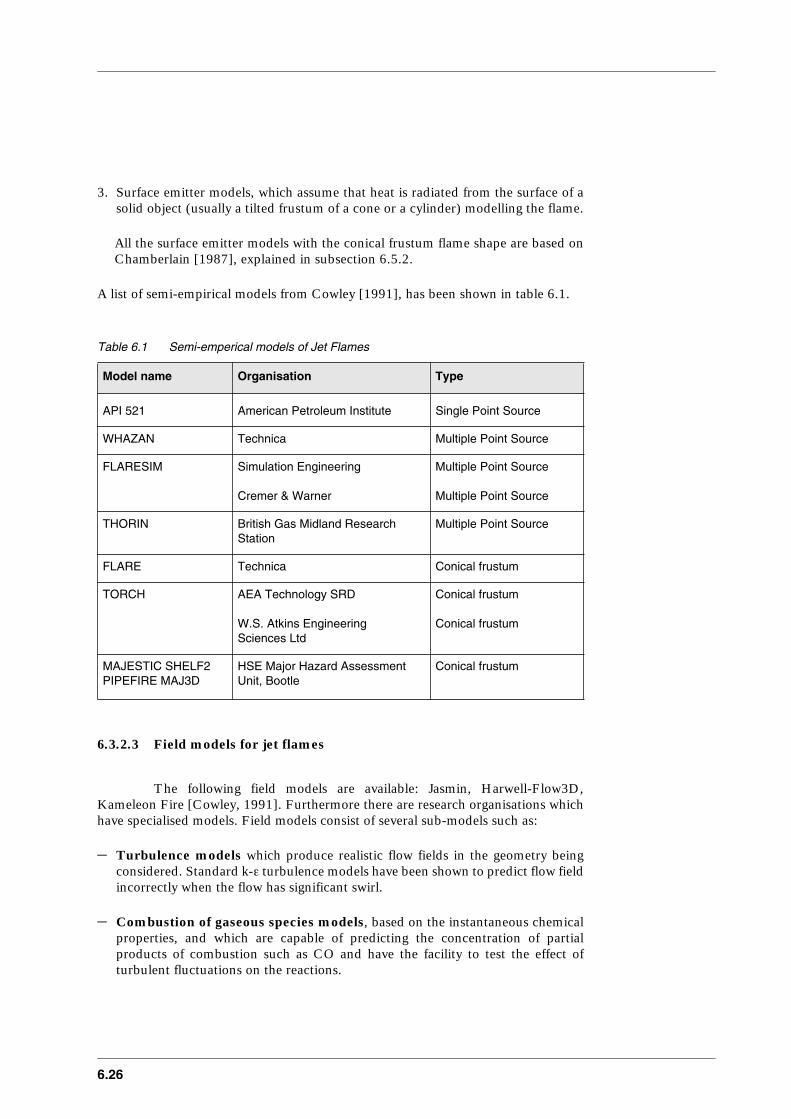
6.26
3. Surface emitter models, which assume that heat is radiated from the surface of asolid object (usually a tilted frustum of a cone or a cylinder) modelling the flame.
All the surface emitter models with the conical frustum flame shape are based onChamberlain [1987], explained in subsection 6.5.2.
A list of semi-empirical models from Cowley [1991], has been shown in table 6.1.
Table 6.1 Semi-emperical models of Jet Flames
6.3.2.3 Field models for jet flames
The following field models are available: Jasmin, Harwell-Flow3D,Kameleon Fire [Cowley, 1991]. Furthermore there are research organisations whichhave specialised models. Field models consist of several sub-models such as:
– Turbulence models which produce realistic flow fields in the geometry beingconsidered. Standard k-ε turbulence models have been shown to predict flow fieldincorrectly when the flow has significant swirl.
– Combustion of gaseous species models, based on the instantaneous chemicalproperties, and which are capable of predicting the concentration of partialproducts of combustion such as CO and have the facility to test the effect ofturbulent fluctuations on the reactions.
Model name Organisation Type
API 521 American Petroleum Institute Single Point Source
WHAZAN Technica Multiple Point Source
FLARESIM Simulation Engineering
Cremer & Warner
Multiple Point Source
Multiple Point Source
THORIN British Gas Midland Research Station
Multiple Point Source
FLARE Technica Conical frustum
TORCH AEA Technology SRD
W.S. Atkins EngineeringSciences Ltd
Conical frustum
Conical frustum
MAJESTIC SHELF2PIPEFIRE MAJ3D
HSE Major Hazard Assessment Unit, Bootle
Conical frustum

CPR 14EChapter 6 of the ‘Yellow Book’
6.27
– Soot production and oxidation models, based on instantaneous speciesconcentrations derived from the gaseous combustion model, hence therequirement to predict partial products of combustion such as OH, which plays amajor role in soot oxidation. Since the timescales of soot reactions are muchlonger than the timescale of gas reactions, the effect of residence time should beincluded in the soot model. Finally, the effects of turbulent fluctuations should betested.
– Radiative heat transfer models, capable of handling non-isothermal, non-homogeneous species distributions, reabsorption of radiation within the flame andthe effect of turbulent fluctuations which are tested.
The requirements for these models are:– The boundary conditions on surfaces and openings should be defined for all the
variables.– Boundary conditions, such as pressure conditions, at openings should not produce
unphysical behaviour in the flow variables.– In most combustion problems, it is necessary to extend the computational grid
well outside the area of interest because of ventilation flows and flame extensions.– Numerical methods should be tested for convergence of computational solutions
and numerical accuracy.
6.3.2.4 Integral models
Earlier integral models ignore the unmixedness of turbulent jet diffusionflames, [Cowley, 1991]. At a given axial position both the flammable material and theair can coexist at the same time in separate turbulent eddies without reacting untilthey are mixed together. The key sub-models in jet fire integral models are similar tothe sub-models for field models of jet fires.Integral models of jet fires from Cowley [1991] are: UPMFIR, TORCIA, THRAINand Cook’s model.Of the integral models only Cook’s model has been validated against large scaleflames. However, even Cook’s integral model does not have its sub-models’validation against data from large-scale experiments because no such data exists.
6.3.3 Impinging fires
6.3.3.1 Introduction
The past 5 to 10 years much attention has been paid to heat impact ofimpinging flames. Two types of impinging jet flames are recognised in literature, viz.the situation in which the object does not perturb the flame, and the situation inwhich the object causes a strong distortion of the flame.
In the literature an overview of appraised work on jet flame impingement up to 1986could be found. Much of the work has been conducted on laboratory flames, burnersand furnaces.

6.28
Cowley (1991) states that soundly based information on heat transfer from large jetfires to engulf objects is lacking. Whilst theoretical models are now beginning toaddress these problems, currently the only reliable method for obtainingimpingement heat flux is direct measurement in flames of adequate size.
6.3.3.2 Fire engulfment of tanks
In the publications Ramskill [1988] and Ramskill [1989] a description ofthe ‘Engulf-II’ is given. In Ramskill [1989] the description was detailed containing allthe mathematical formulae. The models described show that differential equationshave to be solved simultaneously. In the ENGULF-code a fourth order Runge-Kuttaalgorithm is used to calculate the wall temperatures and the bulk vapour and liquidtemperatures.The present code ‘Engulf-II’, can model either total or partial fire engulfment of aLPG-tank, including jet flame impingement. Other features available within the codeare the treatment of safety relief vent valves, bulk boiling of liquid contents, externaltank wall thermal insulation by water spray cooling, tank failure prediction and themodelling of a gas or petrol filled tank. According to Ramskill (1988) the codepredictions have to be in agreement with available experimental data.No field tests were performed but the basics of the models presented are useful.
Computational Fluid Dynamics (CFD) field modelling approaches are particularlyunder development. It is possible that this method is capable of predicting a widerange of impingement conditions. CFD is a sophisticated and powerful technique inwhich the basic physics and chemistry of a flowing fluid can be solved in space andtime. However, there are a large number of unknowns that can only be solved withthe aid of practical data. Run times of these models are in the order of hours. CFDmethods must be regarded as useful adjuncts to the experimental work.
6.3.4 Pool fires on land
6.3.4.1 Introduction
A pool fire can be defined as a turbulent diffusion fire burning above ahorizontal pool vaporising flammable material under conditions where the flammablematerial has zero or very low initial momentum, Cowley [1991].
A key feature of these fires is that there is a degree of feedback between the fire andthe flammable material. To a greater or lesser extent, there is a heat transfer back fromthe fire to the pool that influences or even controls the rate of evaporation and hencethe fire size and other characteristics.The pool with flammable material is not necessarily static. It may be spreading orcontracting. Additional flammable material could be coming from a leak. Depletionof the local flammable material supply can occur via drainage or overflow to otherareas - perhaps giving tide to running liquid fires.The most important parameters for a burning pool which determine the flame shapeare the flame length, flame tilt and the flame drag. The aspect of influence of the wind
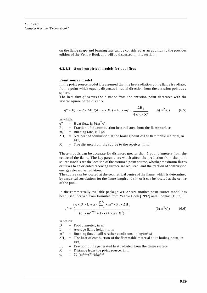
CPR 14EChapter 6 of the ‘Yellow Book’
6.29
on the flame shape and burning rate can be considered as an addition to the previousedition of the Yellow Book and will be discussed in this section.
6.3.4.2 Semi-empirical models for pool fires
Point source modelIn the point source model it is assumed that the heat radiation of the flame is radiatedfrom a point which equally disperses in radial direction from the emission point as asphere.The heat flux q" versus the distance from the emission point decreases with theinverse square of the distance.
q" = Fs × mh' × ∆Hc/(4 × π × X2) = Fs × mh' × (J/(m2⋅s)) (6.5)
in which:q" = Heat flux, in J/(m2⋅s)Fs = Fraction of the combustion heat radiated from the flame surfacemh' = Burning rate, in kg/s∆Hc = Net heat of combustion at the boiling point of the flammable material, in
J/kgX = The distance from the source to the receiver, in m
These models can be accurate for distances greater than 5 pool diameters from thecentre of the flame. The key parameters which affect the prediction from the pointsource models are the location of the assumed point source, whether maximum fluxesor fluxes to an oriented receiving surface are required, and the fraction of combustionenergy released as radiation.The source can be located at the geometrical centre of the flame, which is determinedby empirical correlations for the flame length and tilt, or it can be located at the centreof the pool.
In the commercially available package WHAZAN another point source model hasbeen used, derived from formulae from Yellow Book [1992] and Thomas [1963].
(J/(m2⋅s)) (6.6)
in which:D = Pool diameter, in mL = Average flame height, in mm" = Burning flux at still weather conditions, in kg/(m2⋅s)∆Hc = The heat of combustion of the flammable material at its boiling point, in
J/kgFs = Fraction of the generated heat radiated from the flame surfaceX = Distance from the point source, in mc1 = 72 (m1.22⋅s0.61)/kg0.61
∆Hc
4 π X2××-----------------------
q''π D L π
D2
4------×+××
m× '' Fs ∆Hc××
c1 m''0.61 1+×( ) 4 π X2××( )×----------------------------------------------------------------------------------------=
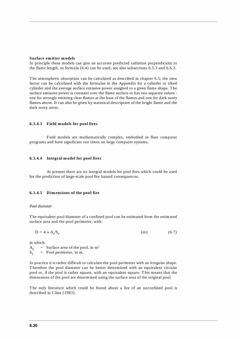
6.30
Surface emitter modelsIn principle these models can give an accurate predicted radiation perpendicular tothe flame length, so formula (6.4) can be used; see also subsections 6.5.3 and 6.6.2.
The atmospheric absorption can be calculated as described in chapter 6.5; the viewfactor can be calculated with the formulae in the Appendix for a cylinder or tiltedcylinder and the average surface emissive power assigned to a given flame shape. Thesurface emissive power is constant over the flame surface or has two separate values -one for strongly emitting clear flames at the base of the flames and one for dark sootyflames above. It can also be given by statistical description of the bright flame and thedark sooty areas.
6.3.4.3 Field models for pool fires
Field models are mathematically complex, embodied in flare computerprograms and have significant run times on large computer systems.
6.3.4.4 Integral model for pool fires
At present there are no integral models for pool fires which could be usedfor the prediction of large-scale pool fire hazard consequences.
6.3.4.5 Dimensions of the pool fire
Pool diameter
The equivalent pool diameter of a confined pool can be estimated from the estimatedsurface area and the pool perimeter, with:
D = 4 × Ap/Sp (m) (6.7)
in which:Ap = Surface area of the pool, in m2
Sp = Pool perimeter, in m.
In practice it is rather difficult to calculate the pool perimeter with an irregular shape.Therefore the pool diameter can be better determined with an equivalent circularpool or, if the pool is rather square, with an equivalent square. This means that thedimensions of the pool are determined using the surface area of the original pool.
The only literature which could be found about a fire of an unconfined pool isdescribed in Cline [1983].
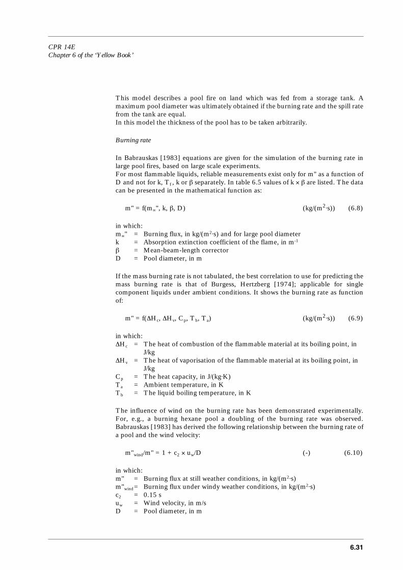
CPR 14EChapter 6 of the ‘Yellow Book’
6.31
This model describes a pool fire on land which was fed from a storage tank. Amaximum pool diameter was ultimately obtained if the burning rate and the spill ratefrom the tank are equal.In this model the thickness of the pool has to be taken arbitrarily.
Burning rate
In Babrauskas [1983] equations are given for the simulation of the burning rate inlarge pool fires, based on large scale experiments.For most flammable liquids, reliable measurements exist only for m" as a function ofD and not for k, Tf , k or β separately. In table 6.5 values of k × β are listed. The datacan be presented in the mathematical function as:
m" = f(m∞", k, β, D) (kg/(m2⋅s)) (6.8)
in which:m∞" = Burning flux, in kg/(m2⋅s) and for large pool diameterk = Absorption extinction coefficient of the flame, in m-1
β = Mean-beam-length correctorD = Pool diameter, in m
If the mass burning rate is not tabulated, the best correlation to use for predicting themass burning rate is that of Burgess, Hertzberg [1974]; applicable for singlecomponent liquids under ambient conditions. It shows the burning rate as functionof:
m" = f(∆Hc, ∆Hv, Cp, Tb, Ta) (kg/(m2⋅s)) (6.9)
in which:∆Hc = The heat of combustion of the flammable material at its boiling point, in
J/kg∆Hv = The heat of vaporisation of the flammable material at its boiling point, in
J/kgCp = The heat capacity, in J/(kg⋅K)Ta = Ambient temperature, in KTb = The liquid boiling temperature, in K
The influence of wind on the burning rate has been demonstrated experimentally.For, e.g., a burning hexane pool a doubling of the burning rate was observed.Babrauskas [1983] has derived the following relationship between the burning rate ofa pool and the wind velocity:
m"wind/m" = 1 + c2 × uw/D (-) (6.10)
in which:m" = Burning flux at still weather conditions, in kg/(m2⋅s)m"wind= Burning flux under windy weather conditions, in kg/(m2⋅s)c2 = 0.15 suw = Wind velocity, in m/sD = Pool diameter, in m
6.32
According to Babrauskas [1983] this is the best available formula, with the restrictionthat it is not applicable for alcohols, nor for conditions under which a fire is blown out(wind velocity > approximately 5 m/s).
Babrauskas [1983] made some remarks on the experimental data which show a slightdecrease in burning rate of very large pools with diameters larger than 5 to 10 metres.It seems that not enough systematic and precise data exist to provide a numericalmodel here, assuming independence of m" on D in this regime. Qualitatively this ispresumed to be due to poorer mixing, leading to a larger cool vapour zone, lowerflame temperatures, and cooler smoke (which can act to shield a fire base from itsflames). In any case, this effect is likely to be larger than about 20%.
Flame length
Many models are proposed in literature. In general for visible flame, length withoutany influence of wind is estimated by the equation from Thomas (1963):
L/D = f(m", ρair, D) (-) (6.11)
in which:m" = Burning rate at still weather conditions, in kg/(m2⋅s)ρair = Density of air, in kg/m3
D = Pool diameter, in m
Under wind blow conditions formula (6.11) becomes a function of u*:
L/D = f(m", ρair, D, u*) (-) (6.12)
with
u* = uw/uc (-) (6.13)
uc = (g × m" × D/ρair)1/3 (m/s) (6.14)
in which:D = pool diameter, in mg = Gravitational acceleration, in m/s2.m" = Burning rate at still weather conditions, in kg/(m2⋅s)ρair = Density of air, in kg/m3
uw = Wind velocity, in m/suc = Characteristic wind velocity, in m/su* = Scaled wind velocity
If uw is less than uc then u* is assigned the value of unity. For wind velocities up to thecharacteristic value, the flame length therefore remains constant whilst at highervalues flame shortening occurs.
It seems that the influence of the wind velocity on the burning rate, as indicated inBabrauskas (1983) has already been incorporated in the Thomas equations. So in theThomas equations the burning rate in still air (uw = 0 m/s) has to be used.
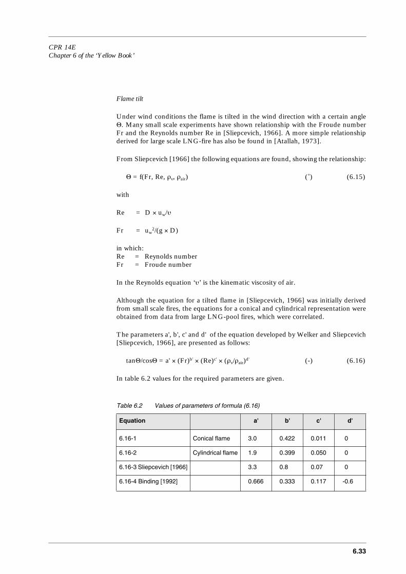
CPR 14EChapter 6 of the ‘Yellow Book’
6.33
Flame tilt
Under wind conditions the flame is tilted in the wind direction with a certain angleΘ. Many small scale experiments have shown relationship with the Froude numberFr and the Reynolds number Re in [Sliepcevich, 1966]. A more simple relationshipderived for large scale LNG-fire has also be found in [Atallah, 1973].
From Sliepcevich [1966] the following equations are found, showing the relationship:
Θ = f(Fr, Re, ρv, ρair) (˚) (6.15)
with
Re = D × uw/υ
Fr = uw2/(g × D)
in which:Re = Reynolds numberFr = Froude number
In the Reynolds equation ‘υ’ is the kinematic viscosity of air.
Although the equation for a tilted flame in [Sliepcevich, 1966] was initially derivedfrom small scale fires, the equations for a conical and cylindrical representation wereobtained from data from large LNG-pool fires, which were correlated.
The parameters a', b', c' and d' of the equation developed by Welker and Sliepcevich[Sliepcevich, 1966], are presented as follows:
tanΘ/cosΘ = a' × (Fr)b' × (Re)c' × (ρv/ρair)d' (-) (6.16)
In table 6.2 values for the required parameters are given.
Table 6.2 Values of parameters of formula (6.16)
Equation a' b' c' d'
6.16-1 Conical flame 3.0 0.422 0.011 0
6.16-2 Cylindrical flame 1.9 0.399 0.050 0
6.16-3 Sliepcevich [1966] 3.3 0.8 0.07 0
6.16-4 Binding [1992] 0.666 0.333 0.117 -0.6
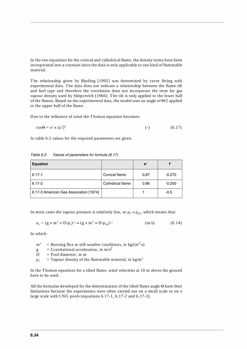
6.34
In the two equations for the conical and cylindrical flame, the density terms have beenincorporated into a constant since the data is only applicable to one kind of flammablematerial.
The relationship given by Binding [1992] was determined by curve fitting withexperimental data. The data does not indicate a relationship between the flame tiltand fuel type and therefore the correlation does not incorporate the term for gasvapour density used by Sliepcevich [1966]. The tilt is only applied to the lower halfof the flames. Based on the experimental data, the model uses an angle of Θ/2 appliedto the upper half of the flame.
Due to the influence of wind the Thomas equation becomes:
cosΘ = e' × (u*)f' (-) (6.17)
In table 6.3 values for the required parameters are given.
Table 6.3 Values of parameters for formula (6.17)
In most cases the vapour pressure is relatively low, so ρv ≈ ρair, which means that:
uc = (g × m" × D/ρv)1/3 ≈ (g × m" × D/ρair)1/3 (m/s) (6.14)
In which:
m" = Burning flux at still weather conditions, in kg/(m2⋅s)g = Gravitational acceleration, in m/s2
D = Pool diameter, in mρv = Vapour density of the flammable material, in kg/m3
In the Thomas equations for a tilted flame, wind velocities at 10 m above the groundhave to be used.
All the formulae developed for the determination of the tilted flame angle Θ have theirlimitations because the experiments were often carried out on a small scale or on alarge scale with LNG pools (equations 6.17-1, 6.17-2 and 6.17-3).
Equation e' f'
6.17-1 Conical flame 0.87 -0.272
6.17-2 Cylindrical flame 0.86 -0.250
6.17-3 American Gas Association [1974] 1 -0.5

CPR 14EChapter 6 of the ‘Yellow Book’
6.35
Flame drag correlation
Due to wind the flame tilts and spills over the edge of a pool or storage tank.Consequently, the flame surface approaches any nearby object on the leeward of thepool, increasing the heat flux of thermal radiation. If wind is hard enough, the flamemay impinge on, for instance, an adjacent tank.
Figure 6.1 shows a schematic representation of the pool diameter D, the flame heightL, and the flame base D' which is elongated due to the effect of wind.
Figure 6.1
Correlation resulting for flames with a conical representation from Moorhouse(1982):
D'/Dw = g' × (Fr)h' × (ρv/ρair)i' (-) (6.18)
In table 6.4 values for the required parameters are given.
Table 6.4 Values of parameters of formula (6.18)
Equation g' h' i'
6.18-1 Conical flame 1.6 0.061 0
6.18-2 Cylindrical flame 1.5 0.069 0
6.18-3 Sliepcevich [1966] 2.1 0.21 0.48
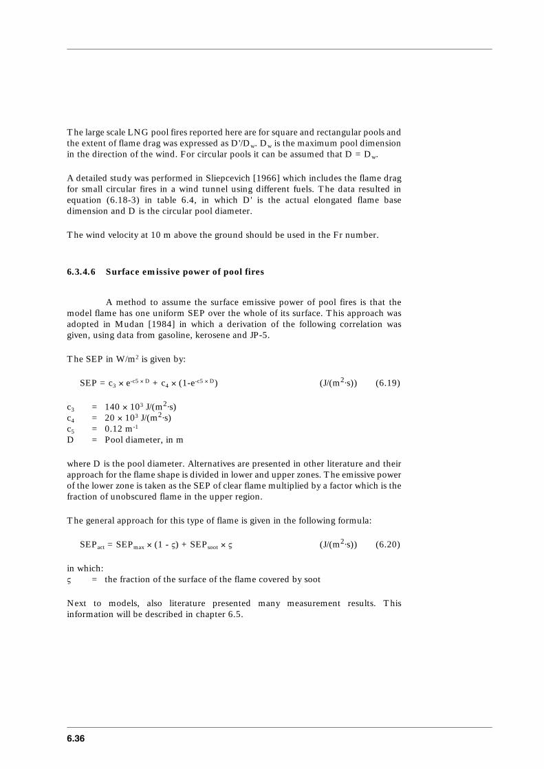
6.36
The large scale LNG pool fires reported here are for square and rectangular pools andthe extent of flame drag was expressed as D'/Dw. Dw is the maximum pool dimensionin the direction of the wind. For circular pools it can be assumed that D = Dw.
A detailed study was performed in Sliepcevich [1966] which includes the flame dragfor small circular fires in a wind tunnel using different fuels. The data resulted inequation (6.18-3) in table 6.4, in which D' is the actual elongated flame basedimension and D is the circular pool diameter.
The wind velocity at 10 m above the ground should be used in the Fr number.
6.3.4.6 Surface emissive power of pool fires
A method to assume the surface emissive power of pool fires is that themodel flame has one uniform SEP over the whole of its surface. This approach wasadopted in Mudan [1984] in which a derivation of the following correlation wasgiven, using data from gasoline, kerosene and JP-5.
The SEP in W/m2 is given by:
SEP = c3 × e-c5 × D + c4 × (1-e-c5 × D) (J/(m2⋅s)) (6.19)
c3 = 140 × 103 J/(m2⋅s)c4 = 20 × 103 J/(m2⋅s)c5 = 0.12 m-1
D = Pool diameter, in m
where D is the pool diameter. Alternatives are presented in other literature and theirapproach for the flame shape is divided in lower and upper zones. The emissive powerof the lower zone is taken as the SEP of clear flame multiplied by a factor which is thefraction of unobscured flame in the upper region.
The general approach for this type of flame is given in the following formula:
SEPact = SEPmax × (1 - ς) + SEPsoot × ς (J/(m2⋅s)) (6.20)
in which:ς = the fraction of the surface of the flame covered by soot
Next to models, also literature presented many measurement results. Thisinformation will be described in chapter 6.5.

CPR 14EChapter 6 of the ‘Yellow Book’
6.37
6.3.5 Pool fires on water
6.3.5.1 Introduction
Studies to model the effects of pool fires on water have, in the first place,been undertaken to evaluate the safety associated with transportation and storage offlammable materials, such as LNG and LPG. More recent studies have been directedtowards the evaluation of combustion of spills of crude and fuel oils on water.
Many additional studies have been undertaken concerning specific topics, such asignition, rate of flame spreading, burning rate and external factors which affectburning rate, effect of weathering and evaporation, heat transfer mechanisms andmodelling. All these studies have generated qualitative results.One model could be found to calculate the burning rate of hydrocarbons on water.
6.3.5.2 Burning rate
Extensive testing was carried out on water to determine the effect of thepool diameter on the burning rate of several crude oils. A compromise was that theoil was burnt in a pan floating in water, so the effect of spreading was neglected.For all fuels tested, the burning rate initially decreased reaching a minimum point andfinally rose to a constant value with an increasing test pan diameter. A constantburning rate was observed for pan diameters > 1 m.
In Petty [1983] seven different crude oils were combusted. The average burning ratein a 2 metre-diameter pans was determined at 5.8·10-2 kg/(m2⋅s). The average burningrates between crude oils do not appear to be a function of a crude oil’s overall specificgravity.
From the test results, a formula was derived to calculate the burning rate; this formulais given in chapter 6.5.
The wind influence on the burning rate was also determined in one of theexperiments and resulted in an increase of the burning rate with a factor 2.
6.3.5.3 Pool diameter
This model of Cline [1983] as mentioned in subsection 6.3.4.5 is intendedfor unconfined pool fires on land.It is assumed that the burning rate in kg/(m2⋅s) is constant; normally the burning rateis a function of the pool diameter.No other models were found in literature, all data describe result of experiments.
6.38
6.3.5.4 Flame height
In Aravamudan [1979] an analytical expression was given to calculate theflame height. However, this equation does not correspond well with the figurespresented.
6.3.5.5 Surface emissive power
For the surface emissive power for pool fires only test results were given.This data was not correlated with formulae.
6.3.6 Fire balls
6.3.6.1 Introduction
In Bagster [1989] an overview was given of the available models for theBLEVE’s with a fireball. The models are exponential relationships to determine thefireball’s diameter and duration. The TNO-model showed the best overall curve fitof the results.The exponent of the relationships seems not to differ too much and is more or lessdependent on the scale of the experiments. A graphical comparison between anumber of models was made with results of accidents and experiments. In somecases, the quantity involved may be overestimated because of prior combustion orleakage.A new development for the calculation of the fraction of generated heat which isradiated is given in subsection 6.3.6.2.
6.3.6.2 Fraction of the generated heat which is radiated
In [Roberts, 1982] the thermal radiation output from a fireball wascharacterised in terms of the fraction of combustion energy released throughradiation, and its dependence on the release pressure. The following relation wasobtained:
Fs = c6 × (Psv)0.32 (-) (6.21)
in which:Fs = Fraction of the generated heat radiated from the flame surfacec6 = 0.00325 (N/m2)0.32
Psv = Saturated vapour pressure before the release, in N/m2
CPR 14EChapter 6 of the ‘Yellow Book’
6.39
6.3.6.3 Lift height of the fire ball
In Cowley [1991] and Bagster [1989] the fireball models have beenevaluated in order to find the best available model. The TNO-model showed the bestoverall curve fit of the results. The formulae include the maximum diameter, durationand the centre height of the fire ball.

6.40
CPR 14EChapter 6 of the ‘Yellow Book’
6.41
6.4 Selection of models
6.4.1 Introduction
In chapter 6.3 all models for the different fire types are addressed.Sometimes a number of different models were found for the same fire type or for thecalculation of different aspects or parameters; in some cases the model is completelynew to the previous edition of the Yellow Book and in other cases it is only an additionor extension.In this chapter 6.4 the selection is made for those models mentioned in chapter 6.3.A choice between models means that criteria have to be used. These criteria are:– degree of validation of the model against experimental data;– complexity of the model.
6.4.2 Jet flames
For jet flames two models were considered because both were validatedwith large scale experiments.One of the models is a centreline trajectory model which is fully described in [Cook,1987]. The model uses difference equations in order to calculate the size and shapeof the flame in small steps. Therefore a computer is necessary to calculate the heatradiation numerically; an analytical solution does not exist for flame models with thecentre line trajectory. This computer model is commercially available as ‘Thorin’.
The other model is a geometric solid flame shape from [Chamberlain, 1987] which isalso validated with large scale experiments, however, it can be programmed moreeasily than the centre line trajectory model. In principle the heat radiation model fora frustum can be calculated analytically. In order to simplify calculations for the viewfactor, the shape of the frustum can even be approximated by a cylinder, by using theaverage diameter of the frustum.
Although the centre line trajectory models may approach the real flame shape betterthan the geometric models, the difference in heat radiation results at a distance seemsto be minor.Both models were validated for a wide range of natural gas experiments, so argumentsof non- or limited validation cannot be used for the selection. Because the calculationof the geometric solid flame model can be made with less computational effort, thismodel has been chosen.
6.4.3 Heat impact of impinging fires
Until now no simple models were available for impinging fires to determinethe heat flux and the temperature rise in steel walls and surfaces exposed to fire.
A thorough description of the heat impact of impinging and engulfing flames has beenpresented in [Ramskill, 1988]. At this moment ‘ENGULF’ can be considered as the
6.42
best attempt to model impingement and engulfment of tanks and vessels. However,other literature sources indicate that there are a large number of unknowns that canonly be clarified by experimental data.
The current results of the tests show until now that the current knowledge andunderstanding in combusting flows is essentially qualitative.At this moment there are no validated predictive tools available that can accuratelydescribe the extent of engulfment and the heat flux distribution over fire impingedobjects.
The model ‘ENGULF’ has not been incorporated, because it is a 3-D model andbecause it has not been validated until now.
6.4.4 Pool fires on land
For heat radiation calculations of a stationary flame shape, the ‘Thomas’-equation (6.11) and the equation (6.9) of Burgess, Hertzberg [1974] can still be used.The ‘Thomas’-equation appears to be adequate for predicting the flame length ofpool fires with a diameter of up to 20 m. The relations which take the influence ofwind into account can be added.
As indicated in Yellow Book [1992] the equivalent diameter of an irregular pool shapecan be determined with the surface area of the pool and the perimeter. It is difficultto estimate the perimeter and therefore it is proposed to calculate the pool diameter,by assuming a circular pool with the same surface area as the original pool. If theshape of the irregular pool can be better compared with a square, then the length ofone side can be calculated.
The equations to calculate Θ (angle of tilting of the flame) are different. The Thomas-equations (6.17-1) and (6.17-2) consistently underpredicts the experimentallyobtained flame tilt angle while equation (6.17-3) tends to overpredict. The equations(6.17-1) and (6.17-2) in table 6.3 are for small scale experiments and equation (6.17-3) is only applicable to large scale LNG fires.
The equations (6.16-1), (6.16-2) and (6.16-3) in table 6.2 for conical and cylindricalflames are based on small scale experiments with different types of flammablematerials, whereas equation (6.16-4) is determined by fitting of experimental data.The data does not incorporate the term for the gas vapour density used by Sliepcevich(1966).In general, equation (6.16-4) is preferred for calculations because it fits experimentaldata.
With equation (6.19) the surface emissive power SEP can be calculated. This formulatakes into account the influence of soot. It has been validated for gasoline, keroseneand JP-5 pool fires. The SEP seems only dependent of the pool diameter.
The view factor for conical and cylindrical flames can be analytically described. In theAppendix the graphical representation as well as the analytical equation arepresented.

CPR 14EChapter 6 of the ‘Yellow Book’
6.43
Furthermore, some experimental results were found in literature and are given inchapter 6.5.
Unconfined poolThe only model for pool fires on land [Cline, 1983], could also be applicable to poolfires on water. With the models the maximum diameter of spreading pool fires can becalculated. The model has not been validated for large scale situations on land.However, it seems to match the small scale measurements well.Some equations (6.78), (6.80) and (6.82) will be given, despite limited validation.
6.4.5 Pool fires on water
No data could be found on the calculation of the flame height. Formulae(6.11) and (6.12) for pool fires on land will be used for pool fires on water.Furthermore, some experimental results were found in literature and are given inchapter 6.5.
6.4.6 Fire balls
In Cowley [1991] and Bagster [1989] fireball models have been evaluatedin order to find the best available model. It can be concluded that (6.90) shows thebest prediction for the whole range of data available from small scale fireballs to largeones. Equations (6.90) and (6.91) which are required for calculation of the fireballdiameter and duration respectively, seem to match the available accidental data offireballs well. The centre height of the fire ball, which belongs to these selectedformulae, is
Hbleve = 2 × rfb (6.22)
according to Bagster [1989].
Equation (6.21) for the calculation of the fraction of the generated heat which isrelated to the saturated vapour pressure, is a useful extension to this model.

6.44

CPR 14EChapter 6 of the ‘Yellow Book’
6.45
6.5 Description of selected models
6.5.1 Introduction
In this chapter, for all fire types a description of the selected models is given.The objective of the selected models is to estimate the heat flux onto an object at acertain distance.The formulae are presented in steps and where necessary an explanation has beengiven. If required, experimental data in tables and figures is given.
6.5.2 Surface emissive power
The important parameters for heat radiation which contribute to the heatload of an object, are:
– Surface Emissive Power (SEP) is the heat radiated outwards per surface area ofthe flame, including the influence of the soot formation (subsection 6.5.2.2).
– View factor Fview (subsection 6.5.2.3) which takes into account:– The shape of the fire, including the influence of wind– Distance of receptor to the outside surface of the fire,– Orientation of the receiving surface (horizontal, vertical and maximum value).
– Atmospheric transmissivity τa (subsection 6.5.2.4).
6.5.2.1 Released heat from combustion
The heat which is generated in a fire depends on the burning rate and theheat of combustion of the flammable material.For modelling a static situation, the shape and the dimensions of the fire are takenconstant, which implies that the supply rate of flammable material is equal to thecombustion rate. The burning rate differs for the various fire types, for instance:
Jet flame: the burning rate under stationary conditions is equal to the release ratein kg/s of the flammable material.
Pool fire: the evaporation rate from the pool is equal to the burning rate.Fire ball: the burning rate is equal to the total amount of flammable material
divided by the duration of the fire ball (which is in fact also the supplyrate).
6.5.2.2 Fraction of the heat radiated
The radiation emittance of materials for which SEPmax has not beenmeasured can be estimated from the combustion energy generated per second, whichcan be determined from the combustion burning-rate and the heat of combustion ofthe material, the surface area of the flame and a fraction of the generated heat which
6.46
is radiated. Hereby it is necessary to select a value of the radiation fraction Fs. Acareful estimation departs from the maximum value found in literature for Fs (see forsome values of Fs in table 6.6 and formulae (6.21) and (6.59)):
SEPmax = Fs × SEPtheor (J/(m2⋅s)) (6.3)
SEPmax = Fs × Q'/A (J/(m2⋅s)) (6.23)
in which:SEPmax = Maximum Surface Emissive Power from a flame without soot
production, in J/(m2⋅s)Q' = Combustion energy per second, in J/sFs = Fraction of the combustion energy radiated from the flame surfaceA = Surface area of the flame, in m2
The Fs factor, in formula (6.3), gives the fraction of the generated heat in the fireemitted by the flame surface in the form of heat radiation. This fraction differs pertype of fire, such as jet flame, pool fire and fire ball, but also depends on the type ofcombustible material.
In contrast to formula (6.3), however, it appears from experiments that the emissivitydecreases with an increase of the flame diameter. Mudan [1984] attributes this to anincreasing formation of black smoke at the flame boundary, such as has beenestablished by hydrocarbons with a molecular ration of carbon: hydrogen bigger than0.3. This black smoke or soot can absorb a great part of the radiation. So the actualvalue of SEPact is less than SEPtheor and SEPmax.
The following formula can be used:
SEPact = SEPmax × (1 - ς) + SEPsoot × ς (J/(m2⋅s)) (6.20)
in which:ς = Fraction of the surface of the flame covered by soot
Hägglund [1976] has found for smoke SEPsoot ≈ 20 × 103 J/(m2⋅s) (in agreement withT ≈ 800 K). Only when such a smoke is not present, the value of SEP calculated fromthe flame temperature must be approximated with formula (6.1).
Mudan [1984] proposes to estimate the emittance of sooting flame surface, assumingthat the major part of the flame (for instance 80%) is enveloped by black smoke andthat there are only certain spots (20%) in which the emittance is maximal.
6.5.2.3 View factor
The geometrical view factor is the ratio between the received and theemitted radiation energy per unit area.The factor is determined by the flame dimensions and shape, and by the relativeposition and orientation of the receiving object.
CPR 14EChapter 6 of the ‘Yellow Book’
6.47
In general, simple flame shapes are taken for the calculations such as sphere, cylinderand flat plate.The view factor of a cylinder can be used for a circular pool fire and a flat plate for asquare or rectangular pool fire. The view factor of a sphere can be used for a fire ball.Practical data and theoretical background of these view factor are given in Appendix.The formula of the view factor becomes more complicated for e.g. a tilted flame, dueto wind influence. For this type of fire a rather complicated analytical solution exists.
6.5.2.4 Atmospheric transmissivity
The atmospheric transmissivity (τa) accounts for the fact that the emittedradiation is partly absorbed by the air present between the radiator and the radiatedobject. The factor is equal to 1 minus the absorption factor, the value which dependson the absorbing properties of the components of the air in relationship to theemission spectrum of the fire. Since water vapour and carbon-dioxide are the mainabsorbing components within the wave length area of the heat radiation, the followingapproximating expression can be given:
τa = 1 - αw - αc (-) (6.24)
Both factors depend on the partial vapour pressure, length L covered by the radiation,the radiator temperature and the ambient temperature. The partial vapour pressureof carbon-dioxide in the atmosphere is normally 30 N/m2, however, the partialvapour pressure of water depends always on the temperature and the relativehumidity.
The absorption takes place in some absorption bands of which the major ones are:
water: 1.8 µm, 2.7 µm, 6.3 µm carbon-dioxide: 2.7 µm, 4.3 µm, 14.4 - 20 µm
Since the energy distribution of the radiation depends on the radiator temperature,the absorption will also be dependent on it. An exact calculation of τa is complicated.
An approximation method on the basis of emission factors given by Hottel [1967] andsummarized by Mudan [1984] is only outlined here:
a. determine the partial vapour pressure of water pw and the length x to be coveredby the radiation in the flame.
b. calculate the reduced vapour pressures.
Pw* = pw × (N/m2) (6.25)
Pc* = pc × (N/m2) (6.26)
in which Tf is the flame or radiator surface temperature and Ta the ambienttemperature.
Tf
Ta------
Tf
Ta------
6.48
c. Determine the emission factors εw (for water vapour) and εc (for carbon-dioxide)for these reduced vapour pressures from the graphs from Hottel [1967], notincluded in this paragraph.
d. Calculate the absorption factors αw (for water vapour) and αc (for carbon-dioxide)from the preceding, in accordance with Welker [1982]:
αw = εw × (Ta/Tf)0.45 (-) (6.27)
αc = εc × (Ta/Tf)0.65 (-) (6.28)
From equations (6.25) and (6.27) we obtain αw as function of Pw* × x, in which x isthe distance from the surface area of the flame to the object, in m; from equations(6.26) and (6.28) we obtain αc, as function of Pc* × x. In order to be able to convertthese functions into values of: αw, as function of pw × x, and αc, as function of pc × x,the temperature Tf must be known.In table 6.5 a number of typical flame temperatures can be found. These values varybetween 800 and 1600 K.If no data is available an average temperature of 1200 K is recommended.
However, for temperatures Tf αw and αc can be estimated directly using the graphsfrom Hottel [1967] which are given in Figures 6.2 and 6.3.The transmissivity τa can be calculated as a function of x, the distance betweenradiator surface and object.
For relative humidities (RH) of 0.4 and 1 and an ‘average’ radiation temperature of1200 K, the transmissivity in Figure 6.4 (in this subsection) has been calculated.
It can be seen from this that differences in relative humidity have little influence on τa
provided τa is expressed as a function of pw × x. The relationship shown is in relativelygood agreement with the graphs given by Raj [1977], which in turn are derived for aradiator temperature of 1150 ˚C, disregarding the carbon-dioxide absorption.
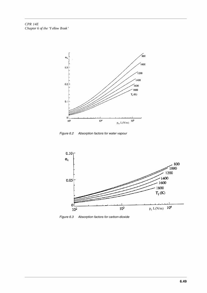
CPR 14EChapter 6 of the ‘Yellow Book’
6.49
Figure 6.2 Absorption factors for water vapour
Figure 6.3 Absorption factors for carbon-dioxide
pw L(N/m)
pc L(N/m)

6.50
Figure 6.4 Transmissivity as a function of the product water vapour pressure pw and length x (radiator temperature 1200 K)
A simple formula was produced [Bagster, 1989], based on data of Figure 6.4, tocalculate the atmospheric transmissivity for all types of fire.
τa = c7 × (pw × x)-0.09 (-) (6.29)
in which:c7 = 2.02 (N/m2)0.09⋅m0.09
pw = Partial water vapour pressure of water in air at a relative humidity RH, inN/m2
x = Distance from the surface area of the flame to the object, in m
This formula can only be used for calculations in the range between:
104 < pw × x < 105 N/m.
In all other cases it is not advised to use (6.29).
6.5.3 Jet flames
In this subsection the model from Chamberlain [1987] has been described.This model, also called ‘Thornton-model’, predicts the flame shape and radiationfield of flares from flare stacks and flare booms. This model has been developed inseveral years of research and has been validated with wind tunnel experiments andfield tests both onshore and offshore. The model represents the flame as a frustum ofa cone, radiating as a solid body with a uniform surface emissive power. Correlationdescribing the variation of flame shape and surface emissive power under a wide rangeof ambient and flow conditions. By increasing the gas exit velocity, the fraction of heatreleased as radiation and the levels of received radiation are reduced. Correlation oflaboratory data and field experience has shown that flames are fully stable under a
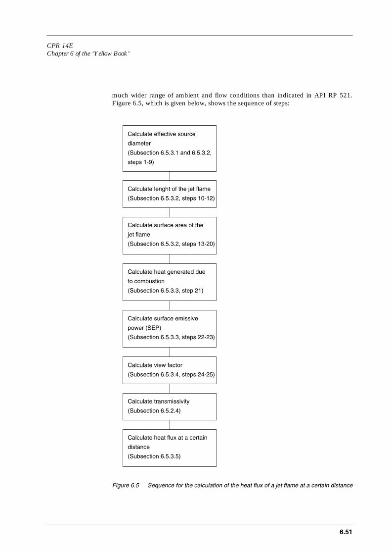
CPR 14EChapter 6 of the ‘Yellow Book’
6.51
much wider range of ambient and flow conditions than indicated in API RP 521.Figure 6.5, which is given below, shows the sequence of steps:
Figure 6.5 Sequence for the calculation of the heat flux of a jet flame at a certain distance
Calculate effective source
diameter
(Subsection 6.5.3.1 and 6.5.3.2,
Calculate lenght of the jet flame
(Subsection 6.5.3.2, steps 10-12)
Calculate surface area of the
jet flame
(Subsection 6.5.3.2, steps 13-20)
Calculate heat generated due
to combustion
(Subsection 6.5.3.3, step 21)
Calculate surface emissive
power (SEP)
(Subsection 6.5.3.3, steps 22-23)
Calculate view factor
(Subsection 6.5.3.4, steps 24-25)
Calculate transmissivity
(Subsection 6.5.2.4)
Calculate heat flux at a certain
distance
(Subsection 6.5.3.5)
steps 1-9)

6.52
The flow diagram for the calculation of the heat flux at a certain distance of a jet flamecan be divided into five parts, viz.:
– Calculation of the exit velocity of the expanding jet;– Calculation of the dimension of the flame;– Calculation of the surface emissive power (SEP);– Calculation of the view factor;– Calculation of the heat flux at a certain distance.
6.5.3.1 Calculation of the exit velocity of the expanding jet
Step 1 to 6 show the calculation of the exit velocity of an expanding jet. Thisexit velocity is an important parameter for the calculation of the flame length, lift-offand the widths of the frustum. First the properties of the flammable material arerequired for the calculation of the exit velocity of the gas, i.e.: molecular weight, thePoisson constant and the storage conditions of the gas, such as temperature andpressure.
Step 1Determine the mass fraction of flammable material in a stoichiometric mixture withair:
W = Wg/(15.816 × Wg + 0.0395) (-) (6.30)
in which:Wg = Molecular weight of gas, in kg/mol
Step 2Calculate Poisson constant γ
γ = Cp/Cv (-) (6.31)
For a so-called ‘ideal gas’
Cv = Cp - Rc/Wg (J/(kg⋅K)) (6.32)
in which:Cp = Specific heat capacity at constant pressure, in J/(kg⋅K)Cv = Specific heat capacity at constant volume, in J/(kg⋅K)Rc = Gas constant 8.314 J/(mol⋅K)
However, for high pressure gas, it is necessary to calculate γ more accurately by usingequation (6.31).
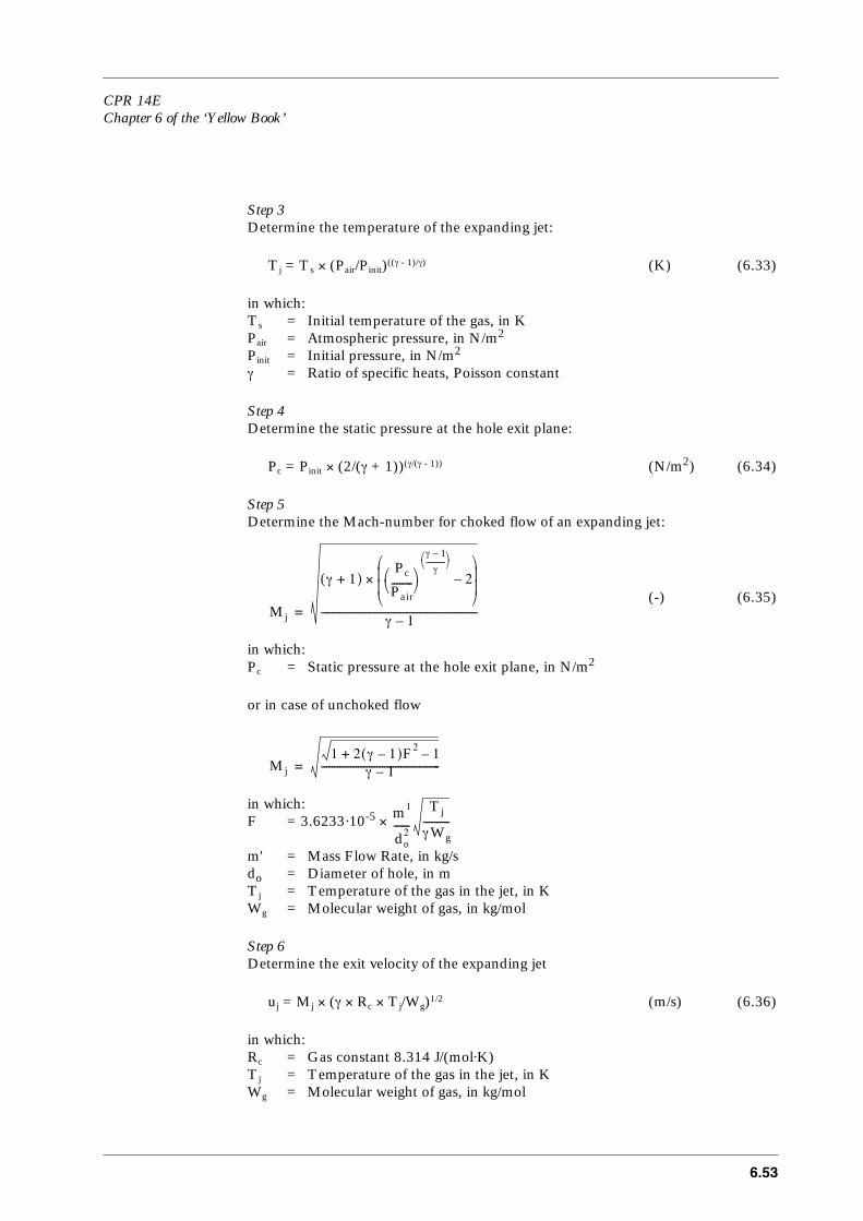
CPR 14EChapter 6 of the ‘Yellow Book’
6.53
Step 3Determine the temperature of the expanding jet:
Tj = Ts × (Pair/Pinit)((γ - 1)/γ) (K) (6.33)
in which:Ts = Initial temperature of the gas, in KPair = Atmospheric pressure, in N/m2
Pinit = Initial pressure, in N/m2
γ = Ratio of specific heats, Poisson constant
Step 4Determine the static pressure at the hole exit plane:
Pc = Pinit × (2/(γ + 1))(γ/(γ - 1)) (N/m2) (6.34)
Step 5Determine the Mach-number for choked flow of an expanding jet:
(-) (6.35)
in which:Pc = Static pressure at the hole exit plane, in N/m2
or in case of unchoked flow
in which:F = 3.6233·10-5 ×
m' = Mass Flow Rate, in kg/sdo = Diameter of hole, in mTj = Temperature of the gas in the jet, in KWg = Molecular weight of gas, in kg/mol
Step 6Determine the exit velocity of the expanding jet
uj = Mj × (γ × Rc × Tj/Wg)1/2 (m/s) (6.36)
in which:Rc = Gas constant 8.314 J/(mol⋅K)Tj = Temperature of the gas in the jet, in KWg = Molecular weight of gas, in kg/mol
Mj
γ 1+( )Pc
Pair--------
γ 1–
γ----------
2–
×
γ 1–-----------------------------------------------------------=
Mj
1 2 γ 1–( )F2 1–+γ 1–---------------------------------------------=
m1
do2
------Tj
γWg
----------
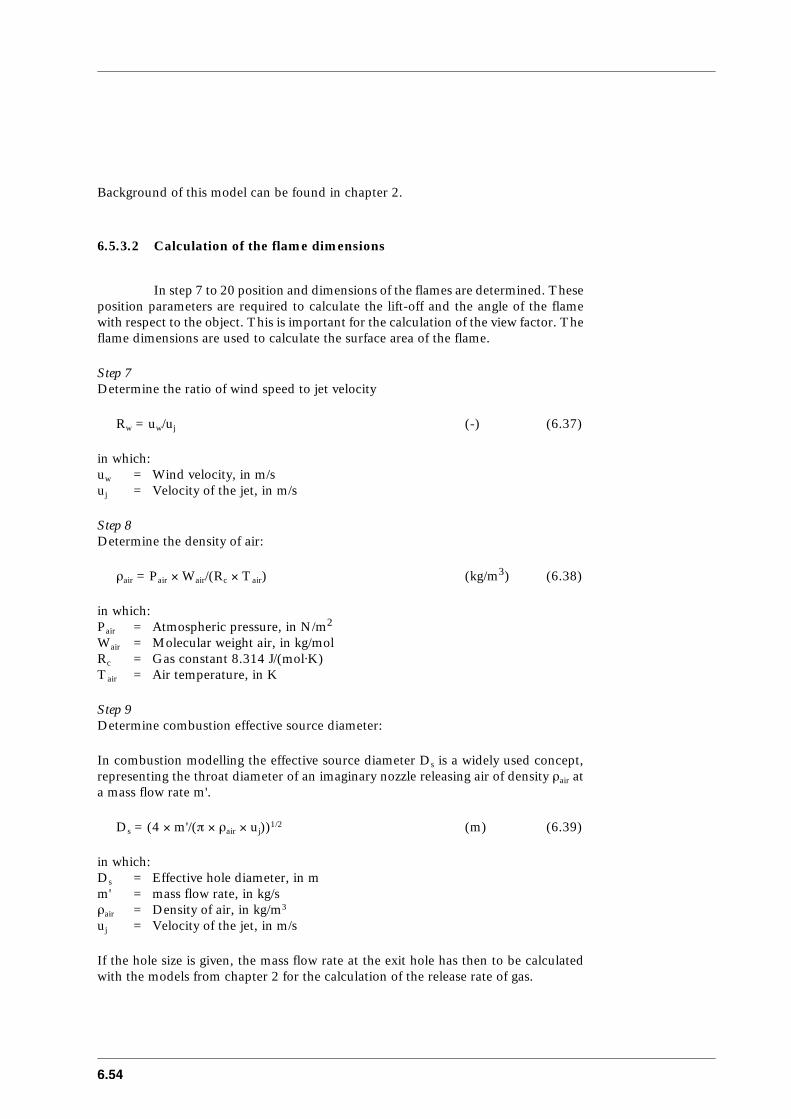
6.54
Background of this model can be found in chapter 2.
6.5.3.2 Calculation of the flame dimensions
In step 7 to 20 position and dimensions of the flames are determined. Theseposition parameters are required to calculate the lift-off and the angle of the flamewith respect to the object. This is important for the calculation of the view factor. Theflame dimensions are used to calculate the surface area of the flame.
Step 7Determine the ratio of wind speed to jet velocity
Rw = uw/uj (-) (6.37)
in which:uw = Wind velocity, in m/suj = Velocity of the jet, in m/s
Step 8Determine the density of air:
ρair = Pair × Wair/(Rc × Tair) (kg/m3) (6.38)
in which:Pair = Atmospheric pressure, in N/m2
Wair = Molecular weight air, in kg/molRc = Gas constant 8.314 J/(mol⋅K)Tair = Air temperature, in K
Step 9Determine combustion effective source diameter:
In combustion modelling the effective source diameter Ds is a widely used concept,representing the throat diameter of an imaginary nozzle releasing air of density ρair ata mass flow rate m'.
Ds = (4 × m'/(π × ρair × uj))1/2 (m) (6.39)
in which:Ds = Effective hole diameter, in mm' = mass flow rate, in kg/sρair = Density of air, in kg/m3
uj = Velocity of the jet, in m/s
If the hole size is given, the mass flow rate at the exit hole has then to be calculatedwith the models from chapter 2 for the calculation of the release rate of gas.
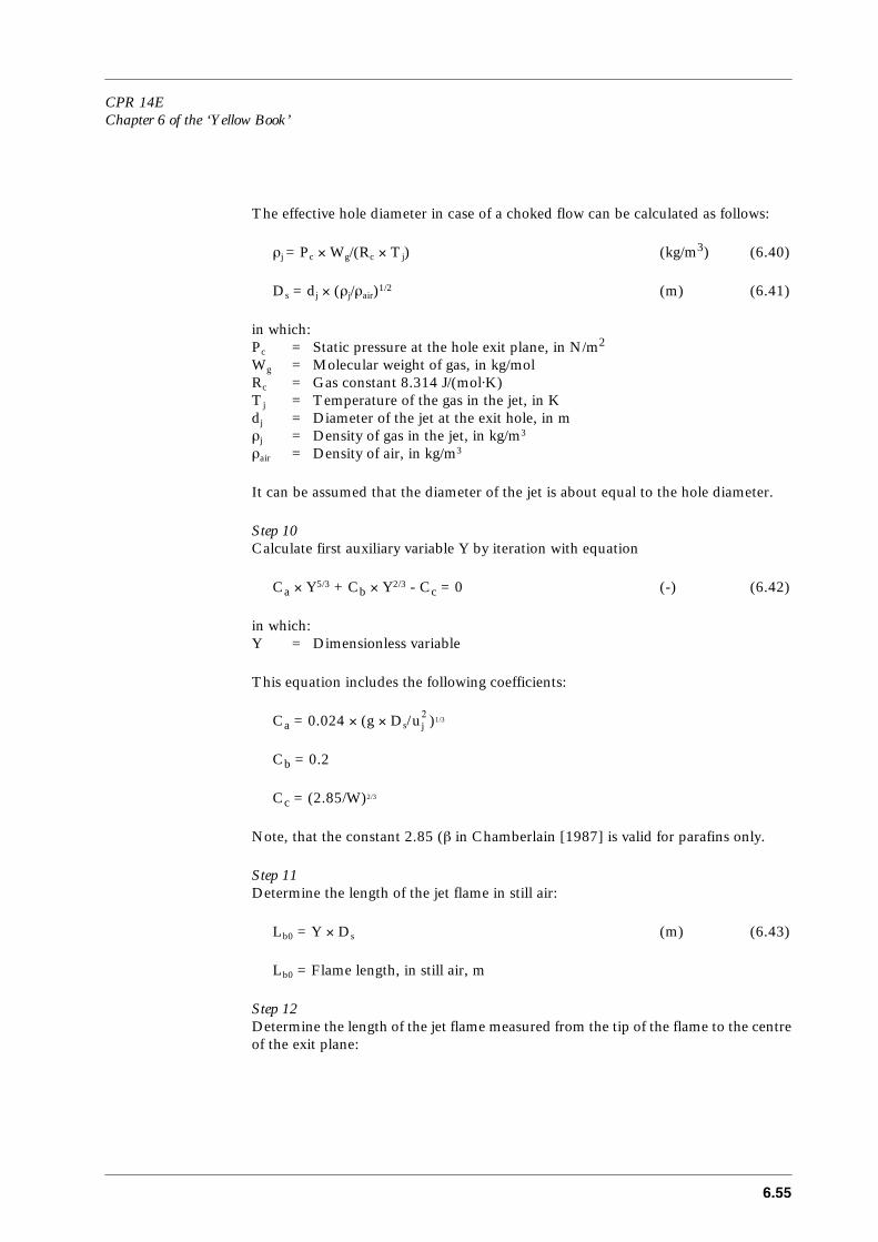
CPR 14EChapter 6 of the ‘Yellow Book’
6.55
The effective hole diameter in case of a choked flow can be calculated as follows:
ρj = Pc × Wg/(Rc × Tj) (kg/m3) (6.40)
Ds = dj × (ρj/ρair)1/2 (m) (6.41)
in which:Pc = Static pressure at the hole exit plane, in N/m2
Wg = Molecular weight of gas, in kg/molRc = Gas constant 8.314 J/(mol⋅K)Tj = Temperature of the gas in the jet, in Kdj = Diameter of the jet at the exit hole, in mρj = Density of gas in the jet, in kg/m3
ρair = Density of air, in kg/m3
It can be assumed that the diameter of the jet is about equal to the hole diameter.
Step 10Calculate first auxiliary variable Y by iteration with equation
Ca × Y5/3 + Cb × Y2/3 - Cc = 0 (-) (6.42)
in which:Y = Dimensionless variable
This equation includes the following coefficients:
Ca = 0.024 × (g × Ds/ )1/3
Cb = 0.2
Cc = (2.85/W)2/3
Note, that the constant 2.85 (β in Chamberlain [1987] is valid for parafins only.
Step 11Determine the length of the jet flame in still air:
Lb0 = Y × Ds (m) (6.43)
Lb0 = Flame length, in still air, m
Step 12Determine the length of the jet flame measured from the tip of the flame to the centreof the exit plane:
uj2
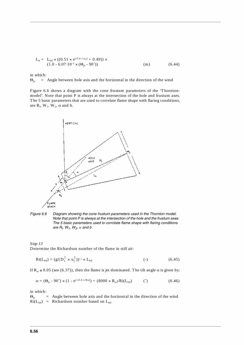
6.56
Lb = Lb0 × ((0.51 × e(-0.4 × uw) + 0.49)) ×(1.0 - 6.07·10-3 × (Θjv - 90˚)) (m) (6.44)
in which:Θjv = Angle between hole axis and the horizontal in the direction of the wind
Figure 6.6 shows a diagram with the cone frustum parameters of the ‘Thornton-model’. Note that point P is always at the intersection of the hole and frustum axes.The 5 basic parameters that are used to correlate flame shape with flaring conditions,are Rl, W1, W2, α and b.
Figure 6.6 Diagram showing the cone frustum parameters used in the Thornton model. Note that point P is always at the intersection of the hole and the frustum axes. The 5 basic parameters used to corrolate flame shape with flaring conditions are Rl, W1, W2, α and b
Step 13Determine the Richardson number of the flame in still air:
Ri(Lb0) = (g/( × ))1/3 × Lb0 (-) (6.45)
If Rw ≤ 0.05 (see (6.37)), then the flame is jet dominated. The tilt angle α is given by:
α = (Θjv - 90˚) × (1 - e(-25.6 × Rw)) + (8000 × Rw)/Ri(Lb0) (˚) (6.46)
in which:Θjv = Angle between hole axis and the horizontal in the direction of the windRi(Lb0) = Richardson number based on Lb0
Lb
Rl
Ds2 uj
2
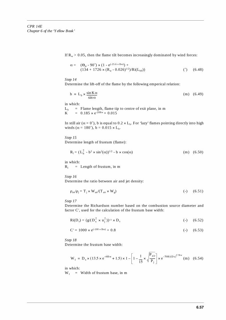
CPR 14EChapter 6 of the ‘Yellow Book’
6.57
If Rw > 0.05, then the flame tilt becomes increasingly dominated by wind forces:
α = (Θjv - 90˚) × (1 - e(-25.6 × Rw)) +(134 + 1726 × (Rw - 0.026)1/2)/Ri(Lb0)) (˚) (6.48)
Step 14Determine the lift-off of the flame by the following emperical relation:
(m) (6.49)
in which:Lb = Flame length, flame tip to centre of exit plane, in mK = 0.185 × e-20Rw + 0.015
In still air (α = 0˚), b is equal to 0.2 × Lb. For ‘lazy’ flames pointing directly into highwinds (α = 180˚), b = 0.015 × Lb.
Step 15Determine length of frustum (flame):
Rl = ( - b2 × sin2(α))1/2 - b × cos(α) (m) (6.50)
in which:Rl = Length of frustum, in m
Step 16Determine the ratio between air and jet density:
ρair/ρj = Tj × Wair/(Tair × Wg) (-) (6.51)
Step 17Determine the Richardson number based on the combustion source diameter andfactor C', used for the calculation of the frustum base width:
Ri(Ds) = (g/( × ))1/3 × Ds (-) (6.52)
C' = 1000 × e(-100 × Rw) + 0.8 (-) (6.53)
Step 18Determine the frustum base width:
(m) (6.54)
in which:W1 = Width of frustum base, in m
b LbKαsinαsin
---------------×=
Lb2
Ds2 uj
2
W1 Ds 13.5 e 6Rw– 1.5+×( ) 1 11
15-----
Pair
Pj--------×– e 70Ri Ds( )
C'Rw–×–××=
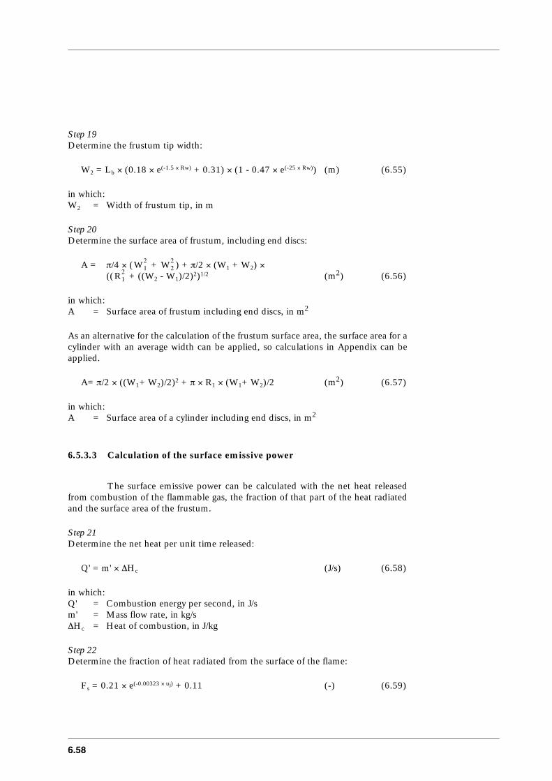
6.58
Step 19Determine the frustum tip width:
W2 = Lb × (0.18 × e(-1.5 × Rw) + 0.31) × (1 - 0.47 × e(-25 × Rw)) (m) (6.55)
in which:W2 = Width of frustum tip, in m
Step 20Determine the surface area of frustum, including end discs:
A = π/4 × ( + ) + π/2 × (W1 + W2) ×(( + ((W2 - W1)/2)2)1/2 (m2) (6.56)
in which:A = Surface area of frustum including end discs, in m2
As an alternative for the calculation of the frustum surface area, the surface area for acylinder with an average width can be applied, so calculations in Appendix can beapplied.
A= π/2 × ((W1+ W2)/2)2 + π × R1 × (W1+ W2)/2 (m2) (6.57)
in which:A = Surface area of a cylinder including end discs, in m2
6.5.3.3 Calculation of the surface emissive power
The surface emissive power can be calculated with the net heat releasedfrom combustion of the flammable gas, the fraction of that part of the heat radiatedand the surface area of the frustum.
Step 21Determine the net heat per unit time released:
Q' = m' × ∆Hc (J/s) (6.58)
in which:Q' = Combustion energy per second, in J/sm' = Mass flow rate, in kg/s∆Hc = Heat of combustion, in J/kg
Step 22Determine the fraction of heat radiated from the surface of the flame:
Fs = 0.21 × e(-0.00323 × uj) + 0.11 (-) (6.59)
W12 W2
2
R12
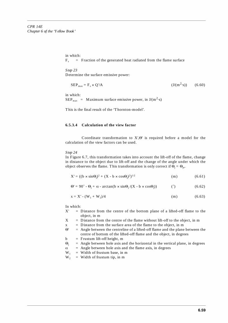
CPR 14EChapter 6 of the ‘Yellow Book’
6.59
in which:Fs = Fraction of the generated heat radiated from the flame surface
Step 23Determine the surface emissive power:
SEPmax = Fs × Q'/A (J/(m2⋅s)) (6.60)
in which:SEPmax = Maximum surface emissive power, in J/(m2⋅s)
This is the final result of the ‘Thornton-model’.
6.5.3.4 Calculation of the view factor
Coordinate transformation to X',Θ' is required before a model for thecalculation of the view factors can be used.
Step 24In Figure 6.7, this transformation takes into account the lift-off of the flame, changein distance to the object due to lift-off and the change of the angle under which theobject observes the flame. This transformation is only correct if Θj = Θjv.
X' = ((b × sinΘj)2 + (X - b × cosΘj)2)1/2 (m) (6.61)
Θ' = 90˚ - Θj + α - arctan(b × sinΘj /(X - b × cosΘj)) (˚) (6.62)
x = X' - (W1 + W2)/4 (m) (6.63)
In which:X' = Distance from the centre of the bottom plane of a lifted-off flame to the
object, in mX = Distance from the centre of the flame without lift-off to the object, in mx = Distance from the surface area of the flame to the object, in mΘ' = Angle between the centreline of a lifted-off flame and the plane between the
centre of bottom of the lifted-off flame and the object, in degreesb = Frustum lift-off height, mΘj = Angle between hole axis and the horizontal in the vertical plane, in degreesα = Angle between hole axis and the flame axis, in degreesW1 = Width of frustum base, in mW2 = Width of frustum tip, in m

6.60
Figure 6.7 Distances, lengths and angles required for the calculation of a lifted-off flame
Step 25Atallah et.al. [1990] show the mathematical formula to calculate the maximum viewfactor of a tilted cylinder at a lift in the direction of the cylinder’s central axis. Thefrustum can be approximated by a cylinder, using the average diameter of thefrustum. In the formulae of the Appendix the value of Θ' and X' can be used in Θ andX to calculate the view factor of a tilted cylinder with the formulae in the Appendix.If the tilt angle of the flame, the radius of the pool/flame, the flame length and thedistance from the flame centre to the object are known, the maximum view factor canbe calculated.It is not allowed to position the object above or under the lifted cylinder, so thedistance of the object from the centre of the flame should be greater than the radiusof the cylinder.
6.5.3.5 Calculation of the heat flux at a certain distance
With the dimensions of the flame and the view factor the thermal heat fluxat a certain distance x from the heat source can be calculated, with:
q"(x) = SEPact × Fview × τa (J/(m2⋅s)) (6.4)
The SEPact is the result of the calculations executed in step 23 in this chapter. Thevalue of the view factor of a tilted cylinder can be calculated with the formulae inAppendix.Both the transmissivity factor τa and the view factor Fview are distance dependent.
frustum
x'
x
b
Θj
Θ'
α
object

CPR 14EChapter 6 of the ‘Yellow Book’
6.61
6.5.4 Pool fires on land
For pool fires on land a number of calculation steps can be distinguished,as is shown in Figure 6.8.
In the heat radiation calculations for pool fire the following main steps can bedistinguished:– Calculation of the liquid pool diameter;– Calculation of the burning rate;– Calculation of the flame dimensions of a pool fire;– Calculation of the surface emissive power;– Calculation of the heat flux at a certain distance.
These steps have been shown in fig. 6.8.
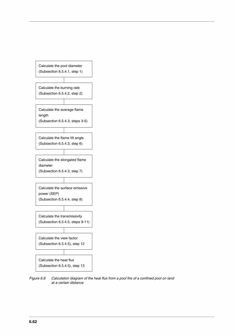
6.62
Figure 6.8 Calculation diagram of the heat flux from a pool fire of a confined pool on land at a certain distance
Calculate the pool diameter
(Subsection 6.5.4.1, step 1)
Calculate the burning rate
(Subsection 6.5.4.2, step 2)
Calculate the average flame
length
(Subsection 6.5.4.3, steps 3-5)
Calculate the flame tilt angle
(Subsection 6.5.4.3, step 6)
Calculate the elongated flame
diameter
(Subsection 6.5.4.3, step 7)
Calculate the view factor
(Subsection 6.5.4.5), step 12
Calculate the surface emissive
power (SEP)
(Subsection 6.5.4.4, step 8)
Calculate the transmissivity
(Subsection 6.5.4.5, steps 9-11)
Calculate the heat flux
(Subsection 6.5.4.5), step 13

CPR 14EChapter 6 of the ‘Yellow Book’
6.63
6.5.4.1 Calculation of the liquid pool diameter
In reality liquid pools will have an irregular shape. In this section themethod is given for transferring this shape into a circular or rectangular pool, whichis required for the calculation of the view factor.
Step 1Determine the pool diameter
For circular pools the heat source can be considered to be cylindrical. In case of arectangular or a nearly rectangular pool, for a ratio length/width smaller than 2, anequivalent or effective pool diameter D can be calculated, which is defined as follows:
Pools with an irregular shape from which the surface area can be determined, can betransformed into a circular pool. The pool diameter can then be calculated with:
D = (4 × Ap/π)1/2 (m) (6.64)
in which:D = Pool diameter, in mAp = Surface area of the pool, in m2
For a length/width ratio larger than 2 (a gutter), an equivalent diameter has to becalculated. The pool fire can thereafter be considered as a flat radiator. The Appendixincludes formulae, numeric values and graphs of the geometric view factor for someradiator configurations.If the released volume and the thickness of the pool can be determined, the circularpool diameter can also be calculated with:
D = (4 × V/(π × δ))1/2 (m) (6.65)
in which:V = Volume of the released liquid, in m3
δ = Thickness of the pool, in m
If the pool is confined in a bund, surface area, length and width are known. This canbe used for calculation of the equivalent pool diameter or the side of an equivalentsquare.
6.5.4.2 Calculation of the burning rate
The burning rate is a function of the pool diameter. However, the influenceof the diameter is only relevant for pools with a diameter smaller than 1 metre.Furthermore the flammable component will have an influence on the amount ofabsorption.Table 6.5 shows burning rates of particular flammable components for largepoolfires. The burning rate of single component liquid flammable material can becalculated with formula (6.9) in step 2a.
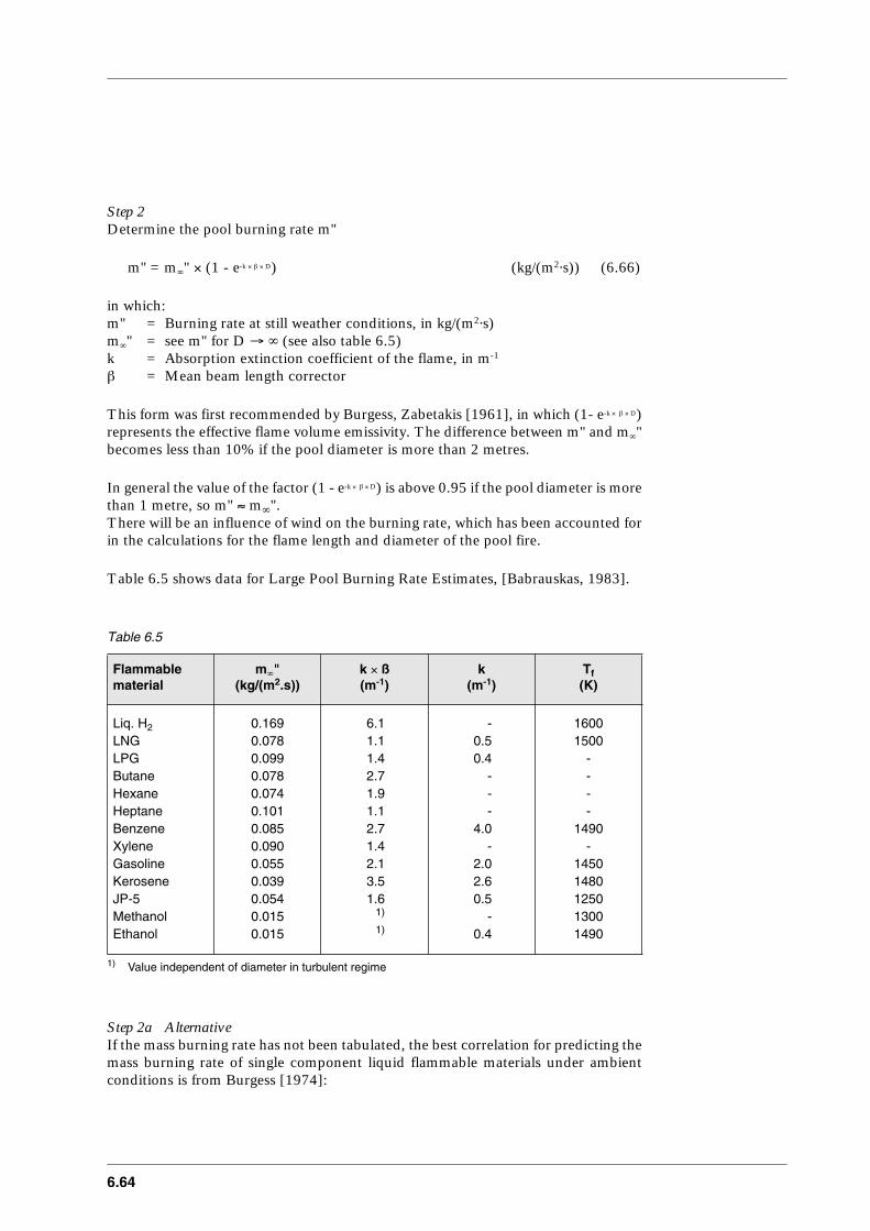
6.64
Step 2Determine the pool burning rate m"
m" = m∞" × (1 - e-k × β × D) (kg/(m2⋅s)) (6.66)
in which:m" = Burning rate at still weather conditions, in kg/(m2⋅s)m∞" = see m" for D → ∞ (see also table 6.5)k = Absorption extinction coefficient of the flame, in m-1
β = Mean beam length corrector
This form was first recommended by Burgess, Zabetakis [1961], in which (1- e-k × β × D)represents the effective flame volume emissivity. The difference between m" and m∞"becomes less than 10% if the pool diameter is more than 2 metres.
In general the value of the factor (1 - e-k × β × D) is above 0.95 if the pool diameter is morethan 1 metre, so m" ≈ m∞".There will be an influence of wind on the burning rate, which has been accounted forin the calculations for the flame length and diameter of the pool fire.
Table 6.5 shows data for Large Pool Burning Rate Estimates, [Babrauskas, 1983].
Table 6.5
Step 2a AlternativeIf the mass burning rate has not been tabulated, the best correlation for predicting themass burning rate of single component liquid flammable materials under ambientconditions is from Burgess [1974]:
Flammable material
m∞"(kg/(m2.s))
k × ß(m-1)
k(m-1)
Tf(K)
Liq. H2
LNGLPGButaneHexaneHeptaneBenzeneXyleneGasolineKeroseneJP-5MethanolEthanol
0.1690.0780.0990.0780.0740.1010.0850.0900.0550.0390.0540.0150.015
6.11.11.42.71.91.12.71.42.13.51.6
1)
1)
1) Value independent of diameter in turbulent regime
-0.50.4
---
4.0-
2.02.60.5
-0.4
16001500
----
1490-
14501480125013001490

CPR 14EChapter 6 of the ‘Yellow Book’
6.65
m" = c8 × ∆Hc/(∆Hv + Cp × (Tb - Ta)) (kg/(m2⋅s)) (6.67)
in which:c8 = 0.001 kg/(m2⋅s)∆Hc = The heat of combustion of the flammable material and its boiling point in
J/kg∆Hv = The heat of vaporisation of the flammable material and its boiling point,
in J/kgCp = The heat capacity in J/(kg⋅K)Tb = The liquid boiling temperature, in KTa = Ambient temperature in K
6.5.4.3 Calculation of the flame dimensions of a pool fire (confined)
The diameter of a pool, which is in first approximation equal to thediameter of the fire, has been calculated in subsection 6.5.4.1. The other dimensionsof a flame will be calculated in this subsection. The influence of wind on flamedimensions will also be considered here. A number of equations have been introducedin this chapter which take that influence into account, so length of the tilted cylinder,the tilt angle of the cylinder and the change of the flame basis are calculated here. Instep 3 to 7 the formulae are given to calculate the dimensions. In step 7 there are twopossibilities given to calculate the flame basis, viz. for a conical and a cylindricalflame.
Step 3Determine the characteristic wind velocity uc
uc = (g × m" × D/ρair)1/3 (m/s) (6.14)
in which:uc = Characteristic wind velocity, in m/sg = Gravitational acceleration 9.81 m/s2
m" = Burning flux in still weather conditions, in kg/(m2⋅s)D = Pool diameter, in m
Step 4Determine the scaled wind velocity u*
u* = uw/uc (-) (6.13)
in which:uw = Wind velocity at height of 10 metres, in m/s
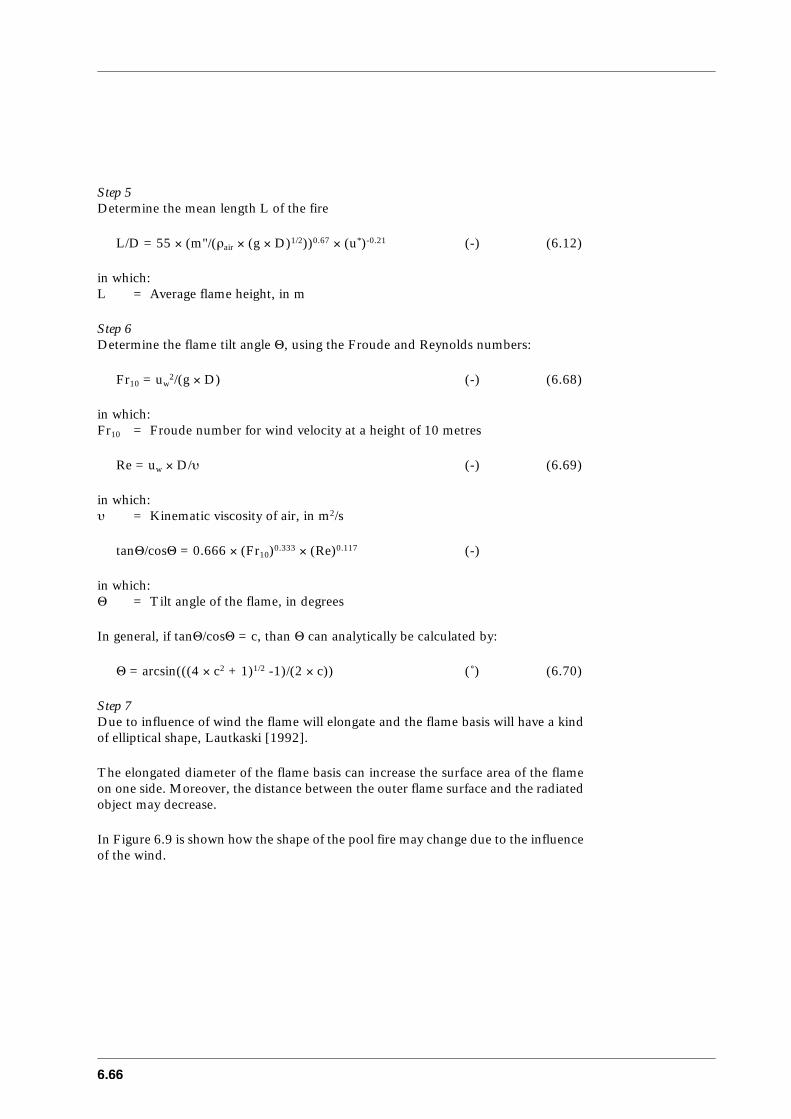
6.66
Step 5Determine the mean length L of the fire
L/D = 55 × (m"/(ρair × (g × D)1/2))0.67 × (u*)-0.21 (-) (6.12)
in which:L = Average flame height, in m
Step 6Determine the flame tilt angle Θ, using the Froude and Reynolds numbers:
Fr10 = uw2/(g × D) (-) (6.68)
in which:Fr10 = Froude number for wind velocity at a height of 10 metres
Re = uw × D/υ (-) (6.69)
in which:υ = Kinematic viscosity of air, in m2/s
tanΘ/cosΘ = 0.666 × (Fr10)0.333 × (Re)0.117 (-)
in which:Θ = Tilt angle of the flame, in degrees
In general, if tanΘ/cosΘ = c, than Θ can analytically be calculated by:
Θ = arcsin(((4 × c2 + 1)1/2 -1)/(2 × c)) (˚) (6.70)
Step 7Due to influence of wind the flame will elongate and the flame basis will have a kindof elliptical shape, Lautkaski [1992].
The elongated diameter of the flame basis can increase the surface area of the flameon one side. Moreover, the distance between the outer flame surface and the radiatedobject may decrease.
In Figure 6.9 is shown how the shape of the pool fire may change due to the influenceof the wind.

CPR 14EChapter 6 of the ‘Yellow Book’
6.67
Figure 6.9 Three common pool geometries with a(a) cylindrical flame, (b) conical flame,(c) cylindrical flame with elongated flame base diameter
Step 7a)
D'/D = 1.6 × (Fr10)0.061 (-) (6.18-1)
for a conical flame presentation
Step 7b)
D'/D = 1.5 × (Fr10)0.069 (-) (6.18-2)
for a cylindrical flame presentation
in which:D = Pool diameter, in mD' = Actual elongated flame base diameter, in m
6.5.4.4 Calculation of the surface emissive power
If the flame dimensions have been determined as well as the heat generatedin the flame due to combustion, the surface emissive power can be calculated.Formula (6.19) is an empirical relationship between the diameter and the surfaceemissive power. In tables 6.7 and 6.8 the surface emissive power has been shown forliquid pools of different components, as well as the ratio of the flame height and thepool diameter. Also the influence of the pool diameter on the surface emissive poweris shown.
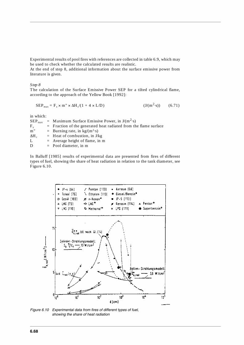
6.68
Experimental results of pool fires with references are collected in table 6.9, which maybe used to check whether the calculated results are realistic.At the end of step 8, additional information about the surface emissive power fromliterature is given.
Step 8The calculation of the Surface Emissive Power SEP for a tilted cylindrical flame,according to the approach of the Yellow Book [1992]:
SEPmax = Fs × m" × ∆Hc/(1 + 4 × L/D) (J/(m2⋅s)) (6.71)
in which:SEPmax = Maximum Surface Emissive Power, in J/(m2⋅s)Fs = Fraction of the generated heat radiated from the flame surfacem" = Burning rate, in kg/(m2⋅s)∆Hc = Heat of combustion, in J/kgL = Average height of flame, in mD = Pool diameter, in m
In Balluff [1985] results of experimental data are presented from fires of differenttypes of fuel, showing the share of heat radiation in relation to the tank diameter, seeFigure 6.10.
Figure 6.10 Experimental data from fires of different types of fuel, showing the share of heat radiation

CPR 14EChapter 6 of the ‘Yellow Book’
6.69
There are, however, two effects which have an impact on the fraction of the generatedcombustion heat, Fs, which is radiated:
a. for small diameters, Fs is clearly smaller than 1,b. for large diameters, soot formation is possible in case of a limited air supply.
In both these cases the SEP will be smaller. It is, therefore rather remarkable that thecombustible substances investigated by Burgess, Hertzberg [1974] (table 6.6):methanol, methane and benzene have a radiation fraction which is practicallyindependent of the pool diameter.
In table 6.6 some experimental values of the fraction of the radiated heat are given.
Table 6.6 Radiation fraction Fs for various poolfires, Burgess, Hertzberg [1974]
The radiation fraction is a factor which generally can only be given with littlecertainty. Its value appears to range between 0.1 and 0.4.
In literature ς = 80% has been found as a representative figure for pool fires of oilproducts
SEPact = SEPmax × (1 - ς) + SEPsoot × ς (J/(m2⋅s)) (6.20)
Substance Pool diameter(m)
Radiation fraction Fs(-)
methanol
methane
butane
gasoline
benzene
0.0760.1521.22
0.3050.761.533.056.10
0.3050.4570.76
1.221.533.05
0.0760.4570.761.22
0.1620.1650.177
0.210.230.15-0.240.24-0.340.20-0.27
0.1990.2050.269
0.30-0.400.16-0.270.13-0.14
0.3500.3450.3500.360
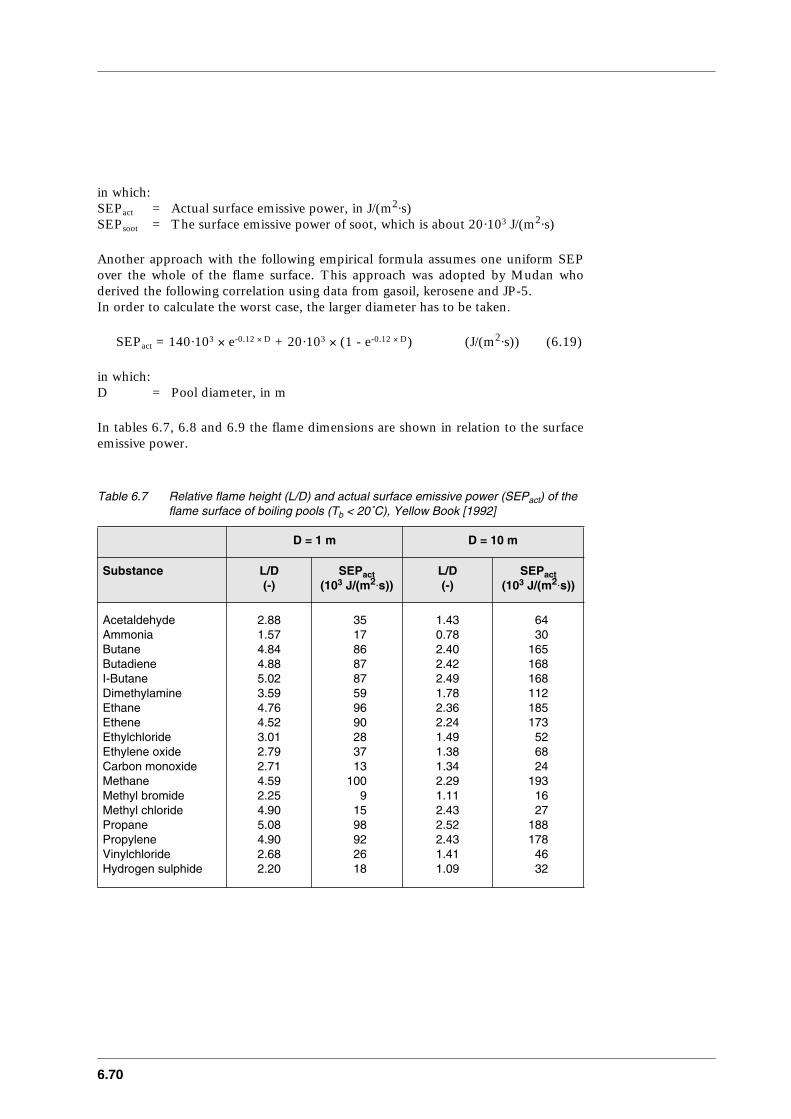
6.70
in which:SEPact = Actual surface emissive power, in J/(m2⋅s)SEPsoot = The surface emissive power of soot, which is about 20·103 J/(m2⋅s)
Another approach with the following empirical formula assumes one uniform SEPover the whole of the flame surface. This approach was adopted by Mudan whoderived the following correlation using data from gasoil, kerosene and JP-5.In order to calculate the worst case, the larger diameter has to be taken.
SEPact = 140·103 × e-0.12 × D + 20·103 × (1 - e-0.12 × D) (J/(m2⋅s)) (6.19)
in which:D = Pool diameter, in m
In tables 6.7, 6.8 and 6.9 the flame dimensions are shown in relation to the surfaceemissive power.
Table 6.7 Relative flame height (L/D) and actual surface emissive power (SEPact) of the flame surface of boiling pools (Tb < 20˚C), Yellow Book [1992]
D = 1 m D = 10 m
Substance L/D(-)
SEPact(103 J/(m2⋅s))
L/D(-)
SEPact(103 J/(m2⋅s))
AcetaldehydeAmmoniaButaneButadieneI-ButaneDimethylamineEthaneEtheneEthylchlorideEthylene oxideCarbon monoxideMethaneMethyl bromideMethyl chloridePropanePropyleneVinylchlorideHydrogen sulphide
2.881.574.844.885.023.594.764.523.012.792.714.592.254.905.084.902.682.20
3517868787599690283713
1009
1598922618
1.430.782.402.422.491.782.362.241.491.381.342.291.112.432.522.431.411.09
6430
165168168112185173526824
1931627
1881784632
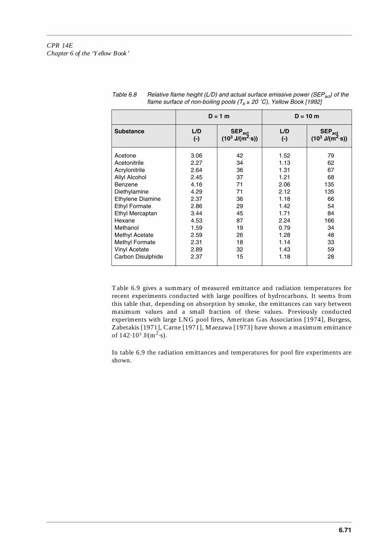
CPR 14EChapter 6 of the ‘Yellow Book’
6.71
Table 6.8 Relative flame height (L/D) and actual surface emissive power (SEPact) of the flame surface of non-boiling pools (Tb ≥ 20 ˚C), Yellow Book [1992]
Table 6.9 gives a summary of measured emittance and radiation temperatures forrecent experiments conducted with large poolfires of hydrocarbons. It seems fromthis table that, depending on absorption by smoke, the emittances can vary betweenmaximum values and a small fraction of these values. Previously conductedexperiments with large LNG pool fires, American Gas Association [1974], Burgess,Zabetakis [1971], Carne [1971], Maezawa [1973] have shown a maximum emittanceof 142·103 J/(m2⋅s).
In table 6.9 the radiation emittances and temperatures for pool fire experiments areshown.
D = 1 m D = 10 m
Substance L/D(-)
SEPact(103 J/(m2⋅s))
L/D(-)
SEPact(103 J/(m2⋅s))
AcetoneAcetonitrileAcrylonitrileAllyl AlcoholBenzeneDiethylamineEthylene DiamineEthyl FormateEthyl MercaptanHexaneMethanolMethyl AcetateMethyl FormateVinyl AcetateCarbon Disulphide
3.062.272.642.454.164.292.372.863.444.531.592.592.312.892.37
4234363771713629458719 26183215
1.521.131.311.212.062.121.181.421.712.240.791.281.141.431.18
79626768
135135665484
1663448335928
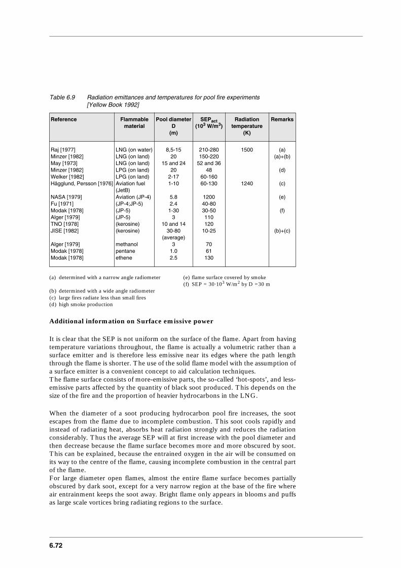
6.72
Table 6.9 Radiation emittances and temperatures for pool fire experiments[Yellow Book 1992]
(a) determined with a narrow angle radiometer (e) flame surface covered by smoke(f) SEP = 30·103 W/m2 by D =30 m
(b) determined with a wide angle radiometer (c) large fires radiate less than small fires(d) high smoke production
Additional information on Surface emissive power
It is clear that the SEP is not uniform on the surface of the flame. Apart from havingtemperature variations throughout, the flame is actually a volumetric rather than asurface emitter and is therefore less emissive near its edges where the path lengththrough the flame is shorter. The use of the solid flame model with the assumption ofa surface emitter is a convenient concept to aid calculation techniques.The flame surface consists of more-emissive parts, the so-called ‘hot-spots’, and less-emissive parts affected by the quantity of black soot produced. This depends on thesize of the fire and the proportion of heavier hydrocarbons in the LNG.
When the diameter of a soot producing hydrocarbon pool fire increases, the sootescapes from the flame due to incomplete combustion. This soot cools rapidly andinstead of radiating heat, absorbs heat radiation strongly and reduces the radiationconsiderably. Thus the average SEP will at first increase with the pool diameter andthen decrease because the flame surface becomes more and more obscured by soot.This can be explained, because the entrained oxygen in the air will be consumed onits way to the centre of the flame, causing incomplete combustion in the central partof the flame.For large diameter open flames, almost the entire flame surface becomes partiallyobscured by dark soot, except for a very narrow region at the base of the fire whereair entrainment keeps the soot away. Bright flame only appears in blooms and puffsas large scale vortices bring radiating regions to the surface.
Reference Flammable material
Pool diameterD
(m)
SEPact(103 W/m3)
Radiationtemperature
(K)
Remarks
Raj [1977]Minzer [1982]May [1973]Minzer [1982]Welker [1982]Hägglund, Persson [1976]
NASA [1979]Fu [1971]Modak [1978]Alger [1979]TNO [1978]JISE [1982]
Alger [1979]Modak [1978]Modak [1978]
LNG (on water)LNG (on land)LNG (on land)LPG (on land)LPG (on land)Aviation fuel(JetB)Aviation (JP-4)(JP-4;JP-5)(JP-5)(JP-5)(kerosine)(kerosine)
methanolpentaneethene
8,5-1520
15 and 2420
2-171-10
5.82.4
1-303
10 and 1430-80
(average)3
1.02.5
210-280150-220
52 and 3648
60-16060-130
120040-8030-50110120
10-25
7061130
1500
1240
(a)(a)+(b)
(d)
(c)
(e)
(f)
(b)+(c)
CPR 14EChapter 6 of the ‘Yellow Book’
6.73
For LPG the average surface emissive power from the present fire was48·103 J/(m2⋅s), only a third of that from the LNG fire. This low average value wasentirely attributable to the soot-masking of the luminous flame. The larger value ofabout 80·103 J/(m2⋅s) was previously obtained from a 1.8 m diameter LPG fire. Thissuggests that the maximum average surface flux for LPG fires occurs close to the pooldiameter at which black soot formation starts to be significant. Further increases inpool diameter will then produce more soot and hence lower average surface fluxes.This was demonstrated more clearly for kerosine. In experiments it was demonstratedthat the SEP of a small kerosine fire of 2 m diameter was about 130·103 J/(m2⋅s) whilethe soot produced in a 10 m pool reduced the SEP to 60·103 J/(m2⋅s). More recentresearch showed for a 20 m pool fire that the SEP reduced to 35·103 J/(m2⋅s), Minzer[1982].
The clear flame length is assumed to be 30% of the total flame length for the pooldiameters larger than 5 m. For pools larger that 25 m in diameter the whole of theflame is assumed to be partially obscured by soot, Cowley [1991].
6.5.4.5 Calculation of the heat flux at a certain distance
For the calculation of the heat flux the transmissivity in the air has to bedetermined. This can be done with the formulae given in subsection 6.5.2.4. First therelative humidity has to be determined. Also formula (6.29) can be used to estimatethe decrease in heat radiation at a certain distance. This is shown in step 11.
Step 9Determine absorption factor for water vapour αw for an average flame temperaturefrom Figure 6.2 (subsection 6.5.2.4), at a certain distance x, between the flamesurface and the object.
Calculate the partial vapour pressure of water pw at Ta and a relative humidity RH.
pw = RH × (N/m2) (6.72)
in which:RH = Relative humidity, fraction between 0 and 1
= Saturated vapour pressure of water in air, in N/m2
Calculate pw × x
From Figure 6.2 αw in relation to pw × x can be found
Step 10Determine the absorption coefficient for carbon-dioxide αc for an average flametemperature from Figure 6.3 (subsection 6.5.2.4) and a distance x, between the flamesurface and target.
Calculate pc × x
From Figure 6.3 αc in relation to pc × x can be found
pwo
pwo

6.74
Step 11Determine the atmospheric transmissivity
τa = 1 - αw - αc (-) (6.24)
or τa can directly be read from Figure 6.4 in subsection 6.5.2.4, or can be calculatedwith:
τa = 2.02 × (pw × x)-0.09 (-) (6.29)
Because pc is constant in air, this can be eliminated in the formula (6.29) as a variableand is included in the constants of the formula.
Step 12Calculate the view factor with the formulae in Appendix. Use the calculated flamedimensions and the distance from the flame to the radiated object as input.
Step 13Calculate the maximum heat flux at a certain distance.
q" = SEPact × Fview × τa (J/(m2⋅s)) (6.4)
6.5.5 Pool fire on land (unconfined)
For unconfined pool fires on land a number of calculations steps can bedistinguished, as shown in Figure 6.11.
In the heat radiation calculations for pool fire the following main steps can bedistinguished:
– Calculation of the liquid pool diameter;– Calculation of the burning rate;– Calculation of the flame dimensions of a pool fire;– Calculation of the surface emissive power;– Calculation of the heat flux at a certain distance.

CPR 14EChapter 6 of the ‘Yellow Book’
6.75
Figure 6.11 Calculation diagram of the heat flux from a pool fire of an unconfined pool on land at a certain distance
Calculate the pool diameter
(Subsection 6.5.5.2, steps 1-10)
Calculate the burning rate
(Subsection 6.5.5.3, steps 12 or
Calculate the average flame
length
(Subsection 6.5.5.3, steps 13-15)
Calculate the flame tilt angle
(Subsection 6.5.3.3, step 16)
Calculate the elongated flame
diameter
(Subsection 6.5.5.3, step 17)
Calculate the surface emissive
(Subsection 6.5.5.4, step 18)
Calculate the transmissivity
(Subsection 6.5.5.5, steps 19-21)
Calculate the view factor
(Subsection 6.5.5.5, step 22)
12a)
power (SEP)
Calculate the heat flux
(Subsection 6.5.5.5, step 23)
Calculate the total release time
and duration of the fire
(Subsection 6.5.5.2, step 11)
6.76
6.5.5.1 Description of the model
In Cline [1983] the pool diameter can be calculated for a burning poolwhich is fed from a storage tank. In the first instance pool diameter and surface areawill increase. The burning rate will also increase with the surface area. At a certainmoment the burning rate is equal to the release rate from the tank, which alsodetermines the maximum pool diameter.This maximum pool diameter can be used for the calculation of the flame height.
The model in its general form is:
2 × π × R × δ × ρ × dR/dt = ρ × A × vf - π × m" × R2 (kg/s) (6.73)
The discharge velocity vf is controlled by the hydrostatic pressure of the fluid level inthe tank. Assuming the fuel tank to discharge through an orifice permits the time-dependent flow velocity to be described by the following relationship:
vf = v0 - a × t (m/s) (6.74)
for: 0 ≤ t ≤ tD,
with
v0 = C0 × (2 × g × hi)1/2 (m/s) (6.75)
where
a = (C0 × A0/At)2 × g (m/s2) (6.76)
In this expression At denotes the cross-sectional area of the tank while hi is the levelof the fluid in the tank in relation to the location of the release area. The burning rateof the liquid m" can be calculated by using the formulae in subsection 6.5.4.2. Theequation above was made dimensionless, using the non-dimensional time τ definedas:
τ = m" × t/(ρ × δ) (-) (6.77)
The dependent variable R can be similarly expressed in a dimensional form as follows:
Φ = m" × π × R2/(ρ × A0 × v0) (-) (6.78)
The non-dimensional form of the pool spread differential equation is:
dΦ/dτ + Φ = 1 - β' × τ (-) (6.79)
The non-dimensional parameter, β', is given by the following relationship:
β' = (a × δ × ρ/(v0 × m")) (-) (6.80)

CPR 14EChapter 6 of the ‘Yellow Book’
6.77
Physically, β' represents the inverse of the non-dimensional time required to dischargethe available fuel load in the tank, i.e., β' = 1/τD.It is important to note that the non-dimensional equation is valid only for thetime interval in which the fuel pool is burning and the tank is releasing fuel, that is τi ≤τ ≤ τD. The lower bound of the time domain, τi, represents an initial condition on thespill at the onset of ignition. The initial condition on the non-dimensional equation istaken as:
Φ(τi) = Φi (-) (6.81)
where Φi is the normalsed pool area at ignition. Solving the non-dimensional equationin conjunction with this condition, leads to the following solution for the transientgrowth of the burning pool fire:
Φ(τ) = 1 + β' × (1 - τ) - [1 - Φi + β' × (1 - τi)] × e-(τ - τi) (-) (6.82)
for: τi ≤ τ ≤ τD
Two situations can be distinguished:1. a fuel pool initially burning, Φ(τi = 0) = 02. a fuel pool with a delayed ignition.For both situations a solution has been given. In case of a fuel pool initially burning,the size of the pool initially increases and after having reached a maximum it willdecrease in size owing to the continually decreasing fuel discharge from the sourcetank. The interior sections of the fuel pool are ‘re-supplied’ with fuel whereas theoutermost edges of the pool become depleted. To satisfy mass conservation the edgesof the pool turn back, resulting in a decrease in pool size. This is presented inFigure 6.12.
Figure 6.12 Normalised Radial Pool Fire Growth - Initially Ignited Pool Fire
'

6.78
Figure 6.13 shows the analytical solution of the ignited pool fire.
Figure 6.13 Normalised Radial Pool Fire Growth - Delayed Ignited Pool Fire
Experiments were carried out to demonstrate the relationship between fuel dischargeand fire size suggested by the present theory. A series of experiments were conductedto measure the time-dependent growth of an unconfined spill fire. Although theexperiments were carried out on a small scale using JP-4 as a fuel, the experimentsshowed that the model described the situation well.No large scale experiments were carried out to validate the model.
6.5.5.2 Calculation of the pool diameter of a pool fire
The following input has been used for the calculation example:At = the cross-sectional area of the tank, in m2
hi = the initial height of the liquid above the release point, in mg = gravitational constant is 9.81 m/s2
C0 = flow coefficient of fluids through a circular holedh = hole diameter of the release point, in mδ = a thickness of the petrol layer on the groundm" = the mass burning flux m" of the petrol at still weather conditions, in
kg/(m2⋅s)ρ = density of petrol, in kg/m3
Φ(τi = 0) = 0, which means that the ignition took place at the beginning of therelease while no liquid pool was present before the release.
Step 1Calculate the surface area A0 of the hole:
'

CPR 14EChapter 6 of the ‘Yellow Book’
6.79
A0 = π/4 × (m2) (6.83)
in which:dh = hole diameter of the release point, in m
Step 2Calculate the initial outflow velocity v0:
v0 = C0 × (2 × g × hi)1/2 (m/s) (6.75)
in which:C0 = flow coefficient of fluids through a circular holeg = gravitational constant is 9.81 m/s2
hi = the initial height of the liquid above the release point, in m
The flow coefficient C0 is the product of a contraction and a friction factor. For asharp-edged orifice the friction factor is nearly 1 and the value of the flow coefficientis fully determined by the contraction factor. In general the value of the flowcoefficient is between 0.6 and 0.8
Step 3Calculate the acceleration constant a:
a = (C0 × A0/At)2 × g (m/s2) (6.76)
in which:At = the cross-sectional area of the tank
Step 4The mass burning rate m" in kg/(m2⋅s) at still weather conditions can be taken fromtable 6.5, or can be calculated with formula (6.66) in subsection 6.5.4.2.
Step 5Calculate the dimensionless parameter τ with:
τ = m" × t/(ρ × δ) (-) (6.77)
in which t remains a variable.
Step 6Calculate the dimensionless parameter Φ with:
Φ = m" × π × R2/(ρ × A0 × v0) (-) (6.78)
in which R remains a variable.
dh2

6.80
Step 7Calculate the dimensionless parameter β' with:
β' = (a × δ × ρ/(v0 × m")) (-) (6.80)
in which:δ = pool thickness, in mρ = liquid density, in kg/m3
Step 8Use the non-dimensional form of the pool spread differential equation, which isapplicable for τi ≤ τ ≤ τD; it is assumed that there is a fire when the release has started,thus Φ(τi = 0) = 0 or Figure 6.12 can be used:
Φ(τ) = 1 + β'(1 - τ) - [1 - Φi + β' (1 - τi)] e-(τ - τi) (-) (6.82)
Step 9Determine the time at which the pool diameter will be maximal.This can be derived from formula (6.82), if dΦ/dτ = 0 is taken. This results in:
τmax = ln((1+β')/β') (-) (6.84)
Furthermore
τ = m" × t/(ρ × δ) (-) (6.77)
in which t remains a variable.
Rearranging formula (6.77) gives:
tmax = τmax × ρ × δ/m" (s)
Step 10Determine the maximum pool diameter at τi = 0 and Φi = 0 and using formula (6.82).
Φmax = 1 + β' × (1 - τmax) - (1 + β') × e-τmax (-) (6.82)
With formula (6.82) the maximum pool radius can be calculated, with:
Φmax = m" × π × /(ρ × A0 × v0) (m) (6.78)
and
Dmax = 2 × Rmax (m)
Now the same calculations can be applied from subsection 6.5.4 to calculate theflame height and the heat flux at a certain distance from the tank.
Rmax2
CPR 14EChapter 6 of the ‘Yellow Book’
6.81
Step 11Determination of the total release time trel and duration of the fire ttot.
The total time of the petrol release from the tank will be:
trel = (At/(C0 × A0)) × (2 × hi/g)1/2 (s) (6.85)
which can be solved from the differential equation:
At × dh/dt = - C0 × A0 × (2 × g × h)1/2 (m3/s)
with h = hi at time t = 0.
The total duration of the fire will be the release time plus the time to burn the petrolin the pool completely.
The time to burn the pool completely after the release has stopped can be derivedfrom:
π × R2 × m" × t = π × R2 × δ × ρ (kg)
which results in
t = δ × ρ/m" (s) (6.86)
ttot = trel + t
ttot = trel + δ × ρ/m" (s) (6.87)
6.5.5.3 Calculation of the flame dimensions of a pool fire
The flame dimension can be calculated in the following steps.
Step 12Determine the pool burning rate m" at still weather conditions
m" = m∞" × (1 - e-k × β × D) (kg/(m2⋅s)) (6.66)
In general the value of the factor (1 - e-k × β × D) is above 0.95 if the pool diameter is morethan 1 metre, so m" ≈ m∞".
Step 12aIf the mass burning rate was not tabulated, the best correlation to use for predictingthe mass burning rate of single component fuels which are liquids under ambientconditions is that of Burgess, Hertzberg [1974]:
m" = 0.001 × ∆Hc/(∆Hv + Cp × (Tb - Ta)) (kg/(m2⋅s)) (6.67)
6.82
Step 13Determine the characteristic wind velocity uc
Uc = (g × m" × D/ρair)1/3 (m/s) (6.14)
Step 14Determine the dimensionless wind velocity u*
u* = uw/uc (-) (6.13)
Step 15Determine the mean fire length
L/D = 55 × (m"/(ρair × (g × D)1/2))0.67 × (u*)0.21 (-) (6.12)
The flame length can now be calculated because D is known.
Step 16Determine the flame tilt angle Θ:
Fr10 = uw2/(g × D) (-) (6.68)
Re = uw × D/υ (-) (6.69)
tanΘ/cosΘ = 0.666 × (Fr10)0.333 × (Re)0.117 (-) (6.16)
In general, if tanΘ/cosΘ = c, then Θ can analytically be calculated by:
Θ = arcsin(((4 × c2 + 1)1/2 -1)/(2 × c)) (˚) (6.70)
Step 17Determine the actual elongated flame base dimension
Step 17a)
D'/D = 1.6 × (Fr10)0.061 (-) (6.18-1)
for a conical flame presentation.
D' can now be calculated, because D is known.
Step 17b)
D'/D = 1.5 × (Fr10)0.069 (-) (6.18-2)
for a cylindrical flame presentation.

CPR 14EChapter 6 of the ‘Yellow Book’
6.83
6.5.5.4 Calculation of the surface emissive power
Step 18Calculate the Surface Emissive Power SEPtheor for a tilted cylindrical flame
SEP = 140·103 × e-0.12 × D + 20·103 × (1 - e-0.12 × D) (J/(m2⋅s)) (6.19)
Table 6.6 can be used to estimate Fs.
SEPmax= Fs × m" × ∆Hc/(1 + 4 × L/D) (J/(m2⋅s)) (6.71)
SEPact = SEPmax × (1 - ς) + SEPsoot × ς (J/(m2⋅s)) (6.20)
6.5.5.5 Calculation of the heat flux at a certain distance
Step 19Determine absorption factor for water vapour αw for an average flame temperature ofTf from Figure 6.2 and for a distance x from the flame surface.
Calculate the partial vapour pressure of water pw at 15 C and a relative humidity RH.
pw = RH × (N/m2) (6.72)
Now pw × x can be calculated.
Figure 6.2 has to be used to find αw.
Step 20Determine the absorption coefficient for carbon-dioxide αc for an average flametemperature of Tf K from Figure 6.3. and a distance x from the flame surface.
Now pc × x can be calculated.
Figure 6.3 has to be used to find αc.
Step 21The calculation with formula (6.24) is generally much more accurate. If the value ofpw × x is between 104 and 105 N/m, formula (6.29) can be used.
Determine the atmospheric transmissivity.
τa = 1 - αw - αc (-) (6.24)
pwo

6.84
Step 22Calculate the view factor with the formulae, shown in Appendix, section 3
a = L/R (-)
b = X/R (-)
A =
B =
C =
D =
E = (a × cos θ)/(b - a × sin θ)
F =
The maximum view factors Fh and Fv can now be calculated with formulae (6.A.14)and (6.A.15), respectively.The maximum view factor can be calculated with formula (6.A.18).
Step 23Calculate the maximum heat flux at a certain distance x
q" = SEPact × Fview × τa (J/(m2⋅s)) (6.4)
6.5.6 Pool fires on water
For pool fires on water a number of calculation steps can be distinguished,as shown in Figure 6.14.
a( 2 b( 1 )+ +2
2 a b 1+( ) θ )sin×××–
a( 2 b 1–( )+2
2 a b 1–( ) θ )sin×××–
1 b2 1–( )+ cos2θ×( )
b 1–( )/ b 1+( )( )
b2 1–( )
Fmax F( v2 Fh
2 )+= (6.A.18)(-)

CPR 14EChapter 6 of the ‘Yellow Book’
6.85
Figure 6.14 Calculation diagram for the heat flux from a pool fire on water at a certain distance
In the heat radiation calculations for pool fire the following steps can bedistinguished:
Calculate the pool diameter
(Subsection 6.5.6.1)
Calculate the burning rate
(Subsection 6.5.6.2)
Calculate the average flame
lenght
(Subsection 6.5.6.3)
Calculate the flame tilt angle
(Subsection 6.5.6.3)
Calculate the elongated flame
diameter
(Subsection 6.5.6.3)
Calculate the surface emissive
(Subsection 6.5.6.4)
Calculate the transmissivity
(Subsection 6.5.6.4)
Calculate heat flux at a certain
distance
(Subsection 6.5.6.4)
power (SEP)
Calculate the view factor
(Subsection 6.5.6.4)

6.86
– Calculation of the liquid pool fire diameter;– Calculation of the burning rate;– Calculation of the flame dimensions of the pool fire;– Calculation of the surface emissive power;– Calculation of the heat flux at a certain distance.
6.5.6.1 Calculation of the liquid pool fire diameter
No models could be found about calculation of the diameter of the liquidpool fire. If the pool on water is confined the equivalent diameter can be calculatedwith equation (6.64). A confined pool can be formed if the perimeter and the surfacearea of the pool do not change in time. This will occur in e.g. harbours when the spillis enclosed by oil booms.
6.5.6.2 Burning rate
In general liquid pools will spread. However, measurements on burningrate are made in controlled conditions with fixed pool diameters.
From literature Petty [1983] the following experimental data have been published intable 6.10.

CPR 14EChapter 6 of the ‘Yellow Book’
6.87
Table 6.10 Mass burning fluxes of flammable materials on water from experiments
Few models can be found in literature about the burning flux of pool fires in water.Most of the available literature is about experimental data.A comparison between the burning flux of crude oils and gasoline in pool fires on landand water does not show much difference.For LPG on water the burning flux is about twice as high as for LPG on land and forLNG this is about three times higher. The differences between the burning flux forthe water and land situation are presented in the following table 6.11.
Table 6.11 Mass burning fluxes for several flammable materials vs. pool diameter and water and land
Flammable material on water
Pool diameter
(m)
Mass burning flux
(kg/(m2⋅s))
Temperature of theflammable material
(˚C)
LPG
LNG
GasolineCrude oil:- Saharan
- Attaka- El Sider- Labuan
- Ekofisk- Isthmus/mayan
- North Slope
- Diesel- Bunker C fuel oil
10.412.916.9
16.8
28.2
2222222222222
0.6290.2400.175
0.255
0.054
0.0560.0470.0570.0480.0430.0430.0650.0730.0470.0690.0610.0510.031
30 5
303030 5
3030 5
30555
Flammable material in water
Pool diameter(m)
Mass burning flux(kg/(m2⋅s))
LPG on land
LPG on water
LNG on landLNG on water
20.012.210.412.914.916.9
up to 16.8up to 13.7
20.035.0
0.130.1360.6290.240.2950.1750.2550.0940.1060.14
6.88
For the calculation of the burning flux on water the following equation can be usedfrom Petty [1983]:
m" = [qrw"/(Q × ln[Bc + 1])] + [(h/Cp) × ln(Bc + 1)] (kg/(m2⋅s)) (6.88)
in which:m" = burning flux in kg/(m2⋅s)qrw"= radiant heat flux to the pool burning surface in J/(m2⋅s).Q = heat of vaporisation in J/kgBc = ‘Spalding’ convection mass transfer numberh = heat transfer coefficient in W/(m2⋅K)Cp = heat capacity in J/(kg⋅K)
The value of Bc ranged from 10.17 to 15.12, so the term ln(Bc+1) varies between 2.41to 2.78, which is a variation of 13%. In general 2.6 can be taken for calculations.
6.5.6.3 Calculation of the flame dimension
The formulae for the calculation of the flame height of a confined pool fireon land, as described in subsection 6.5.4, can be used.
6.5.6.4 Calculation of the heat flux at a certain distance
The heat flux can be calculated in a similar way as for pool fires on land. Inliterature only experimental data could be found with respect to the surface emissivepower. This showed much scatter in the measured SEP’s. No significant differencein SEP between the land and the water situation could be found.The calculations for heat flux at a distance, as described in subsection 6.5.5, can beused.
6.5.7 Fire balls
The calculation steps for the heat flux of a fire ball caused by a BLEVE canbe carried out in four steps, starting from the estimation of the amount of LPG whichwould be involved in a BLEVE.
For the calculation of a fire ball from a BLEVE the following calculation steps arerequired, see Figure 6.15.
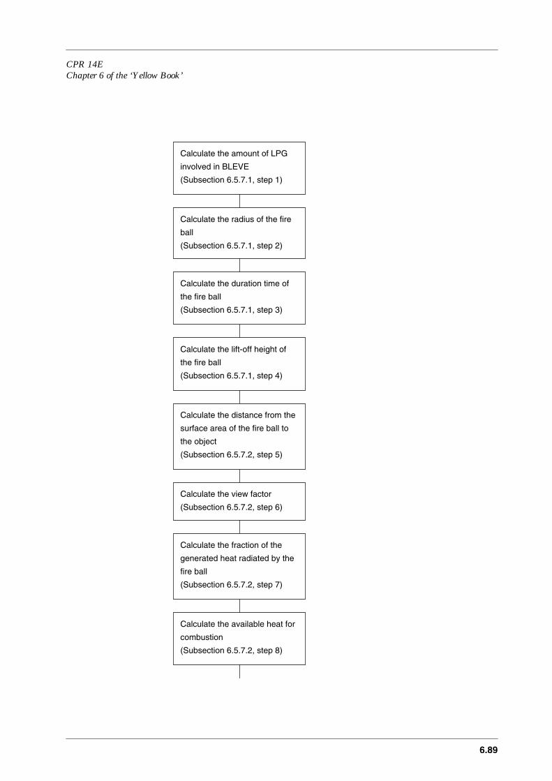
CPR 14EChapter 6 of the ‘Yellow Book’
6.89
Calculate the amount of LPG
involved in BLEVE
(Subsection 6.5.7.1, step 1)
Calculate the radius of the fire
(Subsection 6.5.7.1, step 2)
Calculate the duration time of
the fire ball
(Subsection 6.5.7.1, step 3)
Calculate the lift-off height of
the fire ball
(Subsection 6.5.7.1, step 4)
Calculate the distance from the
(Subsection 6.5.7.2, step 5)
Calculate the view factor
(Subsection 6.5.7.2, step 6)
Calculate the available heat for
combustion
(Subsection 6.5.7.2, step 8)
ball
surface area of the fire ball to
the object
Calculate the fraction of the
(Subsection 6.5.7.2, step 7)
generated heat radiated by the
fire ball

6.90
Figure 6.15 Calculation diagram for the heat flux from a fire ball at a certain distance from the fire ball
6.5.7.1 Calculation of the dimensions, duration and lift-off height
The formulae used for the calculation are given below. In step 2 the releasedamount is ignited and the radius of the fireball can be determined with (6.90); in step3 the duration of a fireball with (6.91) can be calculated and step 4 the centre heightis calculated with equation (6.22). All equations are from TNO [1983].
Step 1Calculate the amount of LPG release in case of a complete failure of the tank
m = Vrel × ρmat = f × V × ρmat (kg) (6.89)
m = Mass of the flammable material, in kgf = Fraction of the volume of the pressure tank, filled with the flammable
liquefied pressurised gasV = Volume of the tank, in m3
Vrel = Amount of e.g. LPG which will be released in case of a complete tank failureρmat = Density of the flammable material in the pressure tank, in kg/m3
Calculate the surface emissive
power (SEP)
(Subsection 6.5.7.2, step 9)
Calculate the distance from the
(Subsection 6.5.7.2, step 10)
Calculate the heat flux at a
certain distance
(Subsection 6.5.7.2, step 14)
centre of the fire ball to the
object
Calculate the transmissivity
(Subsection 6.5.7.2, steps 11-13)
CPR 14EChapter 6 of the ‘Yellow Book’
6.91
Step 2The radius of the fireball can be calculated from the quantity of combusting material:
rfb = c9 × m0.325 (m) (6.90)
In which:c9 = 3.24 m/kg0.325
rfb = Radius of the fireball, in mm = Mass of the flammable material, in kg
Step 3The duration of the fireball is:
t = c10 × m0.26 (s) (6.91)
in which:c10 = 0.852 s/kg0.26
t = Duration of the fireball, in sm = Mass of the flammable material, in kg
Step 4The lift-off height of the fire ball:
Hbleve = 2 × rfb (m) (6.22)
in which:Hbleve = Height from the centre of the fire ball to the ground under the fire ball, in m
6.5.7.2 Calculation of the heat flux at a certain distance
In most literature a uniform heat radiation is assumed. In reality theradiative emission from a fireball varies over its surface. It was found that peakemissions came from areas at the top of the expanding fireball whereas the emissionwas lower from lower portions of the fireball because of increased soot shielding andpoorer mixing with ambient air. They also noted a time dependence of the surfaceemissive power. After an initial period of intense emission there was a gradualdecrease in the SEP. The SEP also varies with fuel type.
For the calculation of the heat flux at a certain distance, parameters such as viewfactor, fraction of the radiated heat and the surface emissive power, are required. Inthe view factor the effects of the distance from the object to the centre of the flameare taken into account.In step 6 the view factor, in step 7 the fraction of the generated heat and in steps 9 theemissive power of the fire ball can be calculated.The heat flux at a certain distance as a result of the calculations can be obtained instep 14.
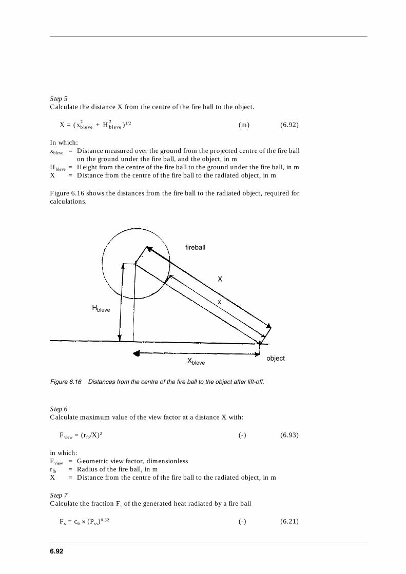
6.92
Step 5Calculate the distance X from the centre of the fire ball to the object.
X = ( + )1/2 (m) (6.92)
In which:xbleve = Distance measured over the ground from the projected centre of the fire ball
on the ground under the fire ball, and the object, in mHbleve = Height from the centre of the fire ball to the ground under the fire ball, in mX = Distance from the centre of the fire ball to the radiated object, in m
Figure 6.16 shows the distances from the fire ball to the radiated object, required forcalculations.
Figure 6.16 Distances from the centre of the fire ball to the object after lift-off.
Step 6Calculate maximum value of the view factor at a distance X with:
Fview = (rfb/X)2 (-) (6.93)
in which:Fview = Geometric view factor, dimensionlessrfb = Radius of the fire ball, in mX = Distance from the centre of the fire ball to the radiated object, in m
Step 7Calculate the fraction Fs of the generated heat radiated by a fire ball
Fs = c6 × (Psv)0.32 (-) (6.21)
xbleve2 Hbleve
2
fireball
Xbleve
Hbleve
object
X
x

CPR 14EChapter 6 of the ‘Yellow Book’
6.93
in which:c6 = 0.00325 (N/m2)0.32
Psv = Vapour pressure of flammable material inside the vessel, in N/m2
Step 8Calculate the nett available heat for radiation
∆H = ∆Hc - ∆Hv - Cp × ∆T (J/kg) (6.94)
in which:∆H = Nett available heat, in J/kg∆Hc = Combustion heat of the flammable material at its boiling point, in J/kg∆Hv = Vaporisation heat of the flammable material at its boiling point, in J/kgCp = Specific heat capacity at constant pressure, J/(kg⋅K)∆T = Temperature difference between flame and ambient temperature, in K
Assume ∆T = 1700 K
Step 9Calculate the Surface Emissive Power SEPact
If it is assumed that there is no soot formation, then SEPact = SEPmax
SEPact = ∆H × m × Fs/(4 × π × × t) (J/(m2⋅s)) (6.95)
in which:SEPact = Actual Surface Emissive Power, SEP, in J/(m2⋅s), which is the average
radiation emittance (emissive power) of the flame surface.SEPmax = Maximum Surface Emissive Power, in J/(m2⋅s).
From the few measurements of the surface emissive powers of fireballs it is reportedthat butane fireballs typically have average SEP values of the visible flame between300·103 and 350·103 J/(m2⋅s). Spot SEPs from highly emissive areas at the top of thefireballs are up to 500·103 J/(m2⋅s).
Step 10Calculate the actual path length between the surface area of the fire ball and theobject.
The actual path length x of radiation from a fire ball is the difference from the centreof the fire ball of the radiated object and distance minus the BLEVE-radius.
x = X - rfb (m) (6.96)
in which:x = Distance from the surface area of the flame to the object, in m
rfb2
6.94
Step 11Determine absorption factor for water vapour αw for an average flame temperature ofTf in K from Figure 6.2, in subsection 6.5.2.4, and for a distance x from the flamesurface.
Calculate the partial vapour pressure of water pw at t ˚C and a relative humidity RH.
pw = RH × (N/m2) (6.72)
Now pw × x can be calculated.
Figure 6.2 has to be used to find αw.
Step 12Determine the absorption coefficient for carbon-dioxide αc for an average flametemperature of Tf in K from Figure 6.3, in subsection 6.5.2.4, and a distance x fromthe flame surface.
Now pc × x can be calculated.
Figure 6.3 has to be used to find αc.
Step 13The calculation with formula (6.24) in general is much more accurate. If the value ofpw × x is between 104 and 105 N/m, formula (6.29) can be used.
Determine the atmospheric transmissivity with
τa = 1 - αw - αc (-) (6.24)
or use Figure 6.4 in subsection 6.5.2.4
Step 13aCalculate the partial vapour pressure of water pw at t ˚C and a relative humidity RH.
pw = RH × (N/m2) (6.72)
An alternative for the calculation of the atmospheric transmissivity τa is formula(6.29)
τa = c7 × (pw × x)-0.09 (-) (6.29)
in which:c7 = 2.02 (N/m2)0.09⋅m0.09
pw = Partial vapour pressure of water in air at a relative humidity RH, in N/m2
x = Distance from the surface area of the flame to the object in m
This formula can only be used for calculations in the range between:
104 < pw × x < 105 N/m.
pwo
pwo

CPR 14EChapter 6 of the ‘Yellow Book’
6.95
Step 14Calculate the heat flux at a certain distance from the centre of fire ball
q" = SEPact × Fview × τa (J/(m2⋅s)) (6.4)
in which:q" = Heat flux at a certain distance, in J/(m2⋅s)τa = Atmospheric transmissivity
For the calculation of the Fview the distance X from the centre of the fire ball to theobject should be used and for the calculation τa the distance x, calculated with (6.96)from the surface area of the fire ball should be used.

6.96

CPR 14EChapter 6 of the ‘Yellow Book’
6.97
6.6 Application of selected models: calculation example
6.6.1 Introduction
In this chapter examples are given of the selected models described inchapter 6.5 of the jet flame, pool fire on land and on water and for the fire ball.The examples are chosen in such a way that these reflect as much as possible theactual situation.The examples are presented in steps in a logical order so the approach can easily betranslated to a computer program.
6.6.2 Jet flames
In this calculation example the heat flux is calculated in 30 steps for anobject at a certain distance from a jet flame.The following input data has been used for the calculation example of a high pressurepipeline (Hole Diameter 100 mm, choked flow) with methane gas:
Wg = 16.042 kg/kmol = 0.016042 kg/molWair = 0.02896 kg/molTs = 15 ˚C = 288.15 KTf = 1200 K = 926.15 °CPair = 1.01325⋅105 N/m2 (1 Bar)Pinit = 107 N/m2 = Pa = 100 BarCp = 2201.6 J/kg⋅KRc = 8.31451 J/mol⋅Kg = 9.80665 m/guw = 5 m/sm' = 30 kg/sΘj = 85˚Θjv = [Θj ≤ Θjv ≤ 90˚], assumption Θjv = 85˚ and wind ⊥ pipe∆Hc = 50·106 J/kgRH = 0.7pw = 1705 N/m2 at 15 ˚Cpc = 30.3975 N/m2 in air (0.03% CO2 in atmosphere)Ta = Ambient temperature 15 ˚C = 288 Kς = 0 (it is assumed that there is no soot formation)X =150 m (Distance release point to receiver)
First the flame dimensions will be calculated and the Surface Emmisive Power (SEP).With this data the maximum heat load at a certain distance of the flame can bedetermined.
6.98
Step 1Determine the mass fraction of fuel in a stoichiometric mixture with air:
W = Wg/(15.816 × Wg + 0.0395) (6.30)= 0.0186/(15.816 × 0.016042 + 0.0395)= 0.05471
Step 2Calculate the Poisson constant γ
Combining formulae (6.31) and (6.32) γ can be calculated with:
γ = (1 - Rc/(Cp × Wg))-1
= (1 - 8.31451/(2201.6 × 0.016042))-1
= 1.30788
(this number will be used in the calculations).
Step 3Determine the temperature of the expanding jet:
Tj = Ts × (Pair/Pinit)((γ - 1)/γ) (6.33)= 288.15 × (1.01325·105/107)((1.30788 - 1)/1.30788)
= 97.758 K
Step 4Determine the static pressure at the hole exit plane:
Pc = Pinit × (2/(γ + 1))(γ/(γ - 1)) (6.34)= 107 × (2/(1.30788 + 1))(1.30788/(1.30788 - 1))
= 5.443070·106 N/m2
Step 5Determine the Mach-number of the expanding jet:
Mj = (((γ + 1) × (Pc/Pair)((γ - 1)/γ) - 2)/(γ - 1))1/2 (6.35)= (((1.30788 + 1) × (5.443·106 N/m2/1.01325·105)((1.30788 - 1)/1.30788) - 2)/(1.30788 - 1))1/2
= 3.55688
Step 6Determine the exit velocity of the expanding jet
uj = Mj × (γ × Rc × Tj/Wg)1/2 (6.36)= 3.55688 × (1.30788 × 8.31451 × 97.758/0.016042)1/2
= 915.60648 m/s

CPR 14EChapter 6 of the ‘Yellow Book’
6.99
Step 7Determine the ratio of wind speed to jet velocity
Rw = uw/uj (6.37)= 5/915.60648= 0.00546
Step 8Determine the density of air:
ρair = (Pair × Wair)/(Rc × Tair) (6.38)= (1.01325·105 × 0.02896)/(8.31451 × 288.15)= 1.224785 kg/m3
Calculate the density in the jet:
Pj = Pc × Wg/(Rc × Tj)= 5.443070·106 × 0.016042/(8.31451 × 97.758) (6.40)= 107.43 kg/m3
Step 9Determine combustion source diameter (choked):
Ds =
= 0.1 (= 100 mm) -
= 0.93656 m
Step 10Calculate first Y by iteration with the equation
Ca × Y5/3 + Cb × Y2/3 - Cc = 0 (6.42)
This involves the following coefficients:
Ca = 0.024 × (g × Ds/ )1/3
= 0.024 × (9.80665 × 0.93656/(915.606482)1/3
= 5.33·10-4
Cb = 0.2
Cc = (2.85/W)2/3
= (2.85/0.05471)2/3
= 13.9482
5.33 ·10-4 × Y5/3 + 0.2 × Y2/3 - 13.9482 = 0
as a result of an iteration, becomes Y = 262.716
dj
Pj
ρair--------×
107.43
1.224785--------------------
uj2
6.100
Step 11Determine the length of the jet flame in still air:
Lb0 = Y × Ds (6.43)= 262.716 × 0.93656= 246.05056 m
Step 12Determine the length of the jet flame measured from the tip of the flame to the centreof the exit plane:
Lb = Lb0 × ((0.51 × e(-0.4 × uw) + 0.49)) × (1.0 - 6.07·10-3 × (Θj - 90˚))= 246.05056 × ((0.51 × e(-0.4 × 5) + 0.49)) × (1.0 - 6.07·10-3 × (85˚ - 90˚))= 141.72199 m (6.44)
Step 13Determine the Richardson number on the flame in still air:
Ri(Lb0) = (g/( × ))1/3 × Lb0 (6.45)Ri(246.05056) = (9.80665/(0.93656)2 × (915.60648)2))1/3 × 246.05056
= 5.8349
Because Rw ≤ 0.05, the flame is jet dominated, and the tilt angle α is given by:
α = (Θjv - 90˚) × (1 - e(-25.6 × Rw)) + 8000 × Rw/Ri(Lb0) (6.46)= (85˚ - 90˚) × (1 - e(-25.6 × 0.00546)) + 8000 × 0.00546/5.8349)= 6.8348
Step 14Determine the lift-off of the flame (b):
K = 0.185 × e-20 Rw+ 0.015= 0.185 × e-20 × 0.0546 + 0.015 = 0.180859
b = Lb × (6.49)
= 141.72199 × =
= 25.69
for α = 0˚ or 180˚ than b is equal to 0.2 × Lb in still air (α = 0˚),or b = 0.015 for ‘lazy’ flames pointing directly into high winds (α = 0˚)
Step 15Determine length of frustum (flame):
Rl = ( - b2 × sin2(α))1/2 - b × cos(α) (6.50)
= =
= 116.18097 m
Ds2 uj
2
Kαsinαsin---------------
0.180859 6.8348×( )sin
6.8348sin-----------------------------------------------------
Lb2
141.72199( )2 25.69( )2– sin2 6.8348( )× 25.69 6.8348( )cos×–
CPR 14EChapter 6 of the ‘Yellow Book’
6.101
Step 16Determine the ratio between air and jet density:
ρair/ρj = Tj × Wair/(Tair × Wg) (6.51)= 97.758 × 0.02896/288.15 × 0.0160428= 0.612424
Step 17Determine the Richardson number based on the combustion source diameter andfactor C', used in calculating the frustum base width:
Ri(Ds) = (g/( × )) × Ds (6.52)Ri(0.1958) = (9.80665/(0.93656)2 × (915.60648)2) × 0.93656
= 0.0222
C' = 1000 × e(-100 × Rw) + 0.8 = 1000 × e-100 × 0.0062 + 0.8 = 580.0123431 (6.53)
Step 18Determine frustum base width:
W1 = Ds × (13.5 × e(-6 × Rw) + 1.5) × (1 - (1 - (ρair/ρj)1/2/15) × )= 0.93656 × (13.5 × e(-6 × 0.00546) + 1.5) × (1 - (1 - (0.6124)1/2/15)
× = 0.71691 m (6.54)
Step 19Determine frustum tip width:
W2 = Lb × (0.18 × e(-1.5 × Rw) + 0.31) × (1 - 0.47 × e(-25 × Rw))= 141.72199 × (0.18 × e(-1.5 × 0.00546) + 0.31) × (1 - 0.47 × e(-25 × 0.00546))= 40.84751 m (6.55)
Step 20Determine the surface area of the frustum, including end discs:
A = π/4 × ( + ) + π/2 × (W1 + W2) × ( + ((W2 - W1)/2)2)1/2
= 3.1416/4 × (0.716912 + 40.847512) + 3.1416/2 ×(0.71691 + 40.84751) × (116.18097)2 + ((40.84751 - 0.71691)/2)2)1/2
= 9008.52 m2 (6.56)
Step 20 aDetermine the surface area of a cylinder with the average of the widths
A = π/2 × ((W1 + W2)/2)2 + π × R1 × (W1 + W2)/2 (6.57)= 3.1416/2 × ((0.71691 + 40.84751)/2)2 + 3.1416 × 116.18097 ×
(0.71691 + 40.84751)/2= 8263.79 m2
Ds2 uj
2 1 3⁄
1 3⁄
e 70 Ri× Ds( )C' Rw×
–
e 70 0.0222×–( )580.01 0.00546×
)
W12 W2
2 R12

6.102
Step 21Determine the net heat released:
Q' = m' × ∆Hc (6.58)= 30 × 50⋅106
= 1.5⋅109 J
Step 22Determine the fraction of heat radiated from the flame surface:
Fs = 0.21 × e(-0.00323 × uj) + 0.11 (6.59)= 0.21 × e(-0.00323 × 915.6064) + 0.11= 0.12091
Step 23Determine the theoretical Surface Emissive Power SEPact:
SEPact = Fs × Q'/A (6.60)
= 0.12091 ×
≈ 21.951⋅103 J/m2⋅s
= 21.951 kW/m2
Step 24Calculate the transformation parameters X', Θ' and x
X' = ((b × sinΘj)2 + (X - b × cosΘj)2)1/2 (6.61)= ((25.69 × sin(85˚))2 + (150 - 25.69 × cos(85˚))2)1/2
= 149.96 m
Θ' = 90˚ - Θj + α - arctan(b × sinΘj /(X - b × cosΘj)) (6.62)= 90˚ - 85 + 6.8348 - arctan(25.69 × sin 85˚/(150 - 25.69 × cos 85˚))= 2.00843
x = X' - (W1 + W2)/4 (6.63)
= 149.96 -
= 139.5698 m
Step 25Calculate the value of the view factor with the formulae presented in Appendix,Section 3, for a tilted cylinder. A tilted cylinder matches the shape of the flame.
At a distance of 46.7 metres from the flame and Θ' of 8.7˚, a view factor of 0.0672 canbe calculated with the formulae from Appendix (see also step 29).
1.5 109⋅
8263.79------------------
0.71691 40.84751+( )
4------------------------------------------------

CPR 14EChapter 6 of the ‘Yellow Book’
6.103
Step 26Calculate the actual Surface Emissive Power SEPact, assuming for a methane flamehardly any soot formation. This means that ς = 0, then
SEPact = SEPmax × (1 - ς) + SEPsoot × ς (6.20)
becomes
SEPact = SEPmax
= 21.951 J/m2⋅s
Step 27Determine absorption factor for water vapour αw for an average flame temperature of1200 K from Figure 6.2 and a distance x of 46.7 metres.
Calculate the partial vapour pressure of water pw at 15 ˚C and a relative humidity RHof 0.7
pw = RH × (6.72)= 0.7 × 1705= 1193.5
pw × x = 1193.5 × 139.5698 = 16.6576·104 N/m
From Figure 6.2, subsection 6.5.2.4, it can be found that αw = 0.2776
Step 28Determine the absorption coefficient for carbon-dioxide αc for an average flametemperature of 1200 K from Figure 6.3 and a distance x of 46.7 metres
pc × x = 30.3975 × 139.5698 = 4.242·103 N/m
From Figure 6.3, subsection 6.5.2.4, it can be found that αc = 0.04941
Step 28aDetermine the atmospheric transmissivity
τa = 1 - αw - αc (6.24)
τa = 1 - 0.2776 - 0.04941 = 0.67302
or Figure 6.4, in subsection 6.5.2.4 can be used
Step 28bAn alternative way of calculating the atmospheric transmissivity
τa = 2.02 × (pw × x)-0.08 (6.29)= 2.02 × (16.6576·104)-0.08
= 0.772
pwo

6.104
There is some difference with the calculated atmospheric transmissivity in step 28b.It is decided that the result of step 28 will be taken for the calculation of the maximumheat flux in step 30.
Step 29Calculate the view factor Fview with the formulae in Appendix, section 3.1
R = (W1 + W2)/4 = (0.71691 + 40.84751)/4 = 10.3911 mX = X' = 149.96 mL = Rl = 116.18097 mΘ = Θ' = 2.00843˚
a = L/R= 116.18097/10.3911 = 11.18
b = X/R= 149.96/10.3911 = 14.43166
A =
=
= 18.736
B =
=
= 17.1724
C =
=
= 14.4228
D =
=
= 0.93295
E = (a × cos θ)/(b - a × sin θ)= (11.18 × cos(2.00843˚))/(14.43166 - 11.18 × sin(2.00843˚))= 0.79587
a2 b 1+( )2 2 a b 1+( ) θsin×××–+( )
11.182 14.43166 1+( )2 2 11.18 14.43166 1+( )× 2.00843˚( )sin××–+( )
a2 b 1–( )2 2 a b 1–( ) θsin×××–+( )
11.182( 14.43166 1–( )2 2 11.18 14.43166 1–( ) 200843˚( ) )sin×××–+
1( b2 1–( ) cos2θ )×+
1( 14.431662 1–( ) cos2 2.00843°( ) )×+
b 1–( )/ b 1+( )( )
14.43166 1–( )( )/ 14.43166 1+( ) )
CPR 14EChapter 6 of the ‘Yellow Book’
6.105
F =
=
= 14.3969
The maximum view factors Fh and Fv can now be calculated with formulae (6.A.14)and (6.A.15), respectively.
Fv = 0.02665
Fh = 0.00934
The maximum view factor can be calculated with formula (6.A.18).
Fmax = (6.A.18)
=
= 0.0282
Step 30Calculate the maximum heat flux at a distance of 49.8 metres from the centre of theflame to the radiated object.
q" = SEPact × Fview × τa (6.4)= 2.1951·104 × 0.0282 × 0.673= 417.236 J/m2s = 0.417 kW/m2
6.6.3 Pool fires on land (confined)
In this calculation example the heat flux is calculated in 13 steps for anobject at a certain distance from a confined pool fire on land.
In this example we consider a pool caused by a release of 28.3 m3 of benzeen with athickness of about 0.02 m.
The following input has been used for the calculation example:
m = ρ⋅V = 882 × 28.3 = 24960 kguw = 5 m/sm∞" = 0.085 kg/m2⋅s (from table 6.2)k × β = 2.7 m-1
υ = kinematic viscosity of air at 15 ˚C, 7.5133·10-6 m2/s (from Annex 1)g = 9.80665 m/s
V = 28.3 m3
δ = 0.02 mA = 1415 m2
b2 1–( )
14.431662 1–( )
F( v2 Fh
2 )+
0.026652 0.009342+( )
6.106
RH = 0.7 = 70%= 1705 N/m2 (RH = 1) at 15 ˚C
pc = 30.3975 N/m2 in air (0.03% CO2 in atmosphere)Ta = Ambient temperature 15 ˚C = 288.15 Kς = 0.8 = 80%∆Hc = 4.015·107 J/kgTb = 80.056 ˚C (= 353.206 K)ρair = 1.2243 kg/m3
x = 100 m (from centre of pool)SEPsoot = 20·103 J/m2·s
Step 1Determine the circular pool diameter:
D = (4 × V/(π × δ))1/2 (6.64)= (4 × 28.3/(3.1416 × 0.02))1/2
= 42.445 m
Step 2Determine the pool burning rate m" at still weather conditions
m" = m∞" × (1 - e-k × β × D) (6.66)= 0.085 × (1 - e- 2.7 × 42.445)= 0.085 kg/(m2⋅s)
In general the value of the factor (1 - e-k × β × D) is above 0.95 if the pool diameter is morethan 1 metre, so m" ≈ m∞".In Annex 1 data can be found to calculate the burning rate of some singlecomponents, which can be used in the calculation of step 2a.
Step 3Determine the characteristic wind velocity uc
uc = (g × m" × D/ρair)1/3 (6.14)= (9.80665 × 0.085 × 42.445/1.2243)1/3
= 3.06866 m/s
Step 4Determine the dimensionless wind velocity u*
u* = uw/uc (6.13)= 5/3.06866= 1.62937
Step 5Determine the mean length of the fire
L/D = 55 × (m"/(ρair × (g × D)1/2))0.67 × (u*)-0.21 (6.12)= 55 × (0.085/(1.2243 × (9.80665 × 42.445)1/2))0.67 × 1.62937-0.21
= 1.101938
pwo
CPR 14EChapter 6 of the ‘Yellow Book’
6.107
L = 1.101938 × D= 1.101938 × 42.445= 46.7725 m
Step 6Determine the flame tilt angle Θ:
Fr10 = uw2/(g × D) (6.68)
= 52/(9.80665 × 42.445)= 0.0545
Re = uw × D/υ (6.69)= 5 × 42.445/7.5133·10-6
= 2.824·107
tanΘ/cosΘ = 0.666 × (Fr10)0.333 × (Re)0.117 (6.16)= 0.666 × (0.0545)0.333 × (2.824·107)0.117
= 1.94315
In general, if tanΘ/cosΘ = c, then Θ can analytically be calculated by:
Θ = arcsin(((4 × c2 + 1)1/2 -1)/(2 × c)) (6.70)= arcsin(((4 × 1.943152 + 1)1/2 -1)/(2 × 1.94315))= 50.8286˚
Step 7Determine the actual elongated flame base dimension
Step 7a)
D'/D = 1.6 × (Fr10)0.061 for a conical flame presentation (6.18-1)= 1.6 × (0.0545)0.061
= 1.3398
D' = 1.3398 × 42.445= 56.867 m
Step 7b)
D'/D = 1.5 × (Fr10)0.069 for a cylindrical flame presentation (6.18-2)= 1.5 × (0.0545)0.069
= 1.2272
D' = 1.2272 × 42.445= 52.0869 m

6.108
Step 8Calculate the Surface Emissive Power SEPtheor for a tilted cylindrical flame
SEP = 140·103 × e-0.12 × D + 20·103 × (1 - e-0.12 × D) (6.19)= 140·103 × e-0.12 × 42.445 + 20·103 × (1 - e-0.12 × 42.445)= 21·103 W/m2
From table 6.6, Fs has been estimated at 0.40
SEPmax = Fs × m" × ∆Hc/(1 + 4 × L/D) (6.71)= 0.40 × 0.085 × 4.015·107/(1 + 4 × 1.101938)= 25.24·104 J/m2⋅s
In literature ς = 80% has been found
SEPact = SEPmax × (1 - ς) + SEPsoot × ς (6.20)= 25.24·104 × (1 - 0.8) + 20·103 × 0.8= 6.6·104 J/m2⋅s
Step 9Determine absorption factor for water vapour αw for an average flame temperature of1200 K from Figure 6.2, in subsection 6.5.2.4, and for a distance x of 50 m from theflame surface.
Calculate the partial vapour pressure of water pw at 15 ˚C and a relative humidity RHof 0.7.
pw = RH × (6.72)= 0.7 × 1705= 1193.5 N/m2
pw × x = 1193.5 × 100= 11.93·104 N/m
From Figure 6.2 it can be found that αw = 0.24513
Step 10Determine the absorption coefficient for carbon-dioxide αc for an average flametemperature of 1200 K from Figure 6.3, subsection 6.5.2.4, and a distance x of 50metres
pc × x = 30.3975 × 100= 3.03975·103 N/m
From Figure 6.3 it can be found that αc = 0.0401285
pwo

CPR 14EChapter 6 of the ‘Yellow Book’
6.109
Step 11The calculation with formula (6.24) is generally much more accurate. If the value ofpw × x is between 104 and 105 N/m, formula (6.29) can be used.
Determine the atmospheric transmissivity
τa = 1 - αw - αc (6.24)= 1 - 0.24513 - 0.0401285= 0.71474
or use Figure 6.4 in subsection 6.5.2.4.
Step 12Calculate the view factor with the formulae from Appendix, section 3
a = L/R= 46.7725/21.222= 2.20396
b = X/R= 100/21.222= 4.712
A =
=
= 4.2384
B =
=
= 2.439498
C =
=
= 3.07555
D =
=
= 0.806135
a2 b 1+( )2 2 a b 1+( ) θsin×××–+( )
2.20396( 2 4.712 1+( )+2
2 2.20396⋅ 4.712 1+( ) 50.8286˚( ) )sin××–
a( 2 b 1–( )2 2 a b 1–( ) θ )sin×××–+
2.20396( 2 4.712 1–( )2 2 2.20396 4.712 1–( ) 50.8286˚( )sin×××–+ )
1( b2 1–( ) cos2θ )×+
1( 4.7122 1–( ) cos2 50.8286˚( ) )×+
b 1–( )/ b 1+( )( )
4.712( 1–( )/ 4.712 1+( ) )
6.110
E = (a × cos θ)/(b - a × sin θ)= (2.20396 × cos(50.8286˚))/(4.712 - 2.20396 × sin(50.828˚))= 0.4635
F =
=
= 4.60457
The maximum view factors Fh and Fv can now be calculated with formulae (6.A.14)and (6.A.15), respectively.
Fv = 0.091915
Fh = 0.029146
The maximum view factor can be calculated with formula (6.A.18).
Fmax = (6.A.18)
=
= 0.0964
Step 13Calculate the maximum heat flux at a distance of 50 metres
q" = SEPact × Fview × τa (6.4)= 6.6·104 × 0.0964 × 0.71474= 4.581·103 J/m2⋅s
6.6.4 Pool fires on land (unconfined)
In this calculation example the heat flux is calculated in 22 steps for anobject at a certain distance from an unconfined pool fire on land.
In this calculation example, we consider a pool caused by an open 4" valve which isconnected with a 196 m3 benzeen storage tank.At some distance of the tank the benzeen is released at ground level. It is assumed thatthe flow resistance in the pipe can be neglected.
b2 1–( )
4.7122 1–( )
F( v2 Fh
2 )+
0.091915( 2 0.029146 )2+
CPR 14EChapter 6 of the ‘Yellow Book’
6.111
The following input has been used for the calculation example:At = 19.63 m2 (diameter of the tank is 5 metres) =
m = ρ·V = 882 × 196 = 172872 kghi = 196 m3/19.6 m2 = 9.98 mg = 9.80665 m/s2
C0 = 0.7dh = 0.1 m = 100 mmm" = m"∞ = 0.085 kg/m2⋅sk × β = 2.7 m-1
ρ = 882 kg/m3
δ = 0.02 m (assumed thickness) = 20 mmΦ(τi = 0) = 0, which means that the ignition took place at the beginning of the
release while no liquid pool was present before the release.υ = 7.513·10-6 m2/s )uw = 5 m/sTf = 1200 KPair = 1.0133·105 N/m2
Pinit = 107 N/m2
γ = 1.4RH = 0.7 = 70%
= 1705 N/m2 (RH = 1) at 15 ˚Cpc = 30.3975 N/m2 (0.03% CO2 in atmosphere)Ta = Ambient temperature 15 ˚C = 288.15 KTb = 80.056 °C (= 353.206 K)ς = 0.8 = 80%∆Hc = 4.015·107 J/kgρair = 1.2243 kg/m3
x = 100 m (from centre of pool)SEPsoot = 20·103 J/m2.s
Step 1Calculate the surface area A0 of the hole:
A0 = π/4 × = 3.1416/4 × 0.12 = π/4 × 0.12
= 0.0079 m2
Step 2Calculate the initial outflow velocity v0:
v0 = C0 × (2 × g × hi)1/2 (6.75)= 0.7 × (2 × 9.80665 × 9.98)1/2
= 9.7935 m/s
π r2⋅ πd
2--- ×
2
π5
2--
2
⋅= =
pwo
dh2

6.112
Step 3Calculate the acceleration constant a:
a = (C0 × A0/At)2 × g (6.76)= (0.7 × 0.0079/19.63)2 × 9.80665= 7.827·10-7 m/s2
Step 4The mass burning rate m" of the petrol at still weather conditions is taken fromtable 6.5.
m" = 0.085 kg/m2⋅s
Step 5Calculate τ
τ = m" × t/(ρ × δ) (6.77)= 0.085 × t/(882 × 0.02)= 4.8185·10-3 × t
Step 6Calculate Φ
Φ = m" × π × R2/(ρ × A0 × v0) (6.78)= 0.085 × 3.1416 × R2/(882 × 0.0079 × 9.7935)= 3.913·10-3 × R2
Step 7Calculate β'
β' = (a × δ × ρ/(v0 × m")) (6.80)= (7.7827·10-7 × 0.02 × 882/(9.7935 × 0.085))= 1.649·10-5
Step 8Use the non-dimensional form of the pool spread differential equation, which isapplicable for τi ≤ τ ≤ τD; it is assumed that there is a fire when the release has started,thus Φ(τi = 0) = 0:
Φ(τ) = 1 + β'(1 - τ) - [1 - Φi + β'( 1 - τi)] e-(τ - τi) (6.82)= 1 + 1.649·10-5 × (1 - τ) - (1 + 1.649·10-5) × e-τ
Step 9Determine the time at which the pool diameter will be maximal.This will be obtained, if dΦ/dτ = 0 and means that:
τmax = ln((1+β')/β') (6.84)= ln((1 + 1.649·10-5)/1.649·10-5)= 11.0128

CPR 14EChapter 6 of the ‘Yellow Book’
6.113
Furthermore
τ = 4.8185·10-3 × t (6.77)
tmax = 11.0128/4.8185·10-3
= 2285 s= 0.63 h
Step 10Determine the maximum pool diameter.
Φmax = 1 + (1.649·10-5 × (1 - 11.0128)) - (1 + 1.649·10-5) × e-11.0128 (6.82)= 1 - 1.6511·10-4 - 1.6489·10-5
= 0.9998
Rmax = (Φ/3.913·10-3)1/2 (6.78)= (0.9998/3.913·10-3)1/2
= 15.985 m
Dmax = 2 × Rmax = 2 × 15.985= 31.97 m
Now the same calculations from subsection 6.6.3 can be applied to calculate theflame height and the heat flux at a certain distance from the tank.
Step 11Determine of the total release time trel and duration of the fire ttot.
The total time of the benzene release from the tank will be:
trel = (At/(C0 × A0)) × (2 × hi/g)1/2 (6.85)= (19.63/(0.7 × 0.0079)) × (2 × 9.98/9.80665)1/2
= 5064 s= 1.41 h
This means that:
τ = 4.8185·10-3 × t (6.77)= 4.8185·10-3 × 5064= 24.40
Formula 6.82 can now be filled in, giving the following result:
Φ = 1 + (1.649·10-5·(1-24.4)) - (1 + 1.649·10-5)e-24.4
= 1 - 3.85866·10-4 - 2.53·10-11 = 0.9996
Because R = (Φ/3.913·10-3)1/2 it means that the pool diameter will not decreasesignificantly between 0.63 and 1.41 h.

6.114
The total duration of the fire will be the release time plus the time to burn the benzenein the pool completely.
ttot = trel + δ × ρ/m" (6.87)= 5064 + 0.02 × (882/0.085)= 5271.5 s= 1.46 h
Step 12Determine the characteristic wind velocity uc
uc = (g × m" × D/ρair)1/3 (6.14)= (9.80665 × 0.085 × 31.97/1.2243)1/3
= 2.792 m/s
Step 13Determine the dimensionless wind velocity u*
u* = uw/uc (6.13)= 5/2.792= 1.79
Step 14Determine the mean length of the fire
L/D = 55 × (m"/(ρair × (g × D)1/2))0.67 × (u*)-0.21 (6.12)= 55 × (0.085/(1.2243 × (9.80665 × 31.97)1/2))0.67 × (1.79)-0.21
= 1.1857
L = 1.1857 × D= 1.1857 × 31.97= 37.91 m
Step 15Determine the flame tilt angle Θ:
Fr10 = uw2/(g × D) (6.68)
= 52/(9.80665 × 37.91)= 0.00799
Re = uw × D/υ (6.69)= 5 × 37.91/7.513·10-6
= 2.12·107
tanΘ/cosΘ = 0.666 × (Fr10)0.333 × (Re)0.117 (6.16)= 0.666 × (0.0799)0.333 × (2.12·107)0.117
= 2.0669

CPR 14EChapter 6 of the ‘Yellow Book’
6.115
In general, if tanΘ/cosΘ = c, then Θ can analytically be calculated by:
Θ = arcsin(((4 × c2 + 1)1/2 -1)/(2 × c)) (6.70)= arcsin(((4 × 2.06692 + 1)1/2 -1)/(2 × 2.0669))= 51.9˚
Step 16Determine the actual elongated flame base dimension
Step 16a)
D'/D = 1.6 × (Fr10)0.061 for a conical flame presentation (6.18-1)= 1.6 × (0.0799)0.061
= 1.371
D' = 1.371 × 31.97= 43.84 m
Step 16b)
D'/D = 1.5 × (Fr10)0.069 for a cylindrical flame presentation (6.18-2)= 1.5 × (0.0799)0.069
= 1.2599
D' = 1.2599 × 31.97= 40.28 m
Step 17Calculate the Surface Emissive Power SEPmax for a tilted cylindrical flame
SEPact = 140·103 × e-0.12 × D + 20·103 × (1 - e-0.12 × D) (6.19)= 140·103 × e-0.12 × 31.97 + 20·103 × (1 - e-0.12 × 31.97)= 3019.96 + 19568.6 = 22.59·103 J/m2⋅s
From table 6.6, Fs has been estimated at 0.40
SEPmax = Fs × m" × ∆Hc/(1 + 4 × L/D) (6.71)= 0.4 × 0.085 × 4.0185·107/(1 + 4 × 1.1857)= 23.72·104 J/m2⋅s
In literature ς = 80% has been found
SEPact = SEPmax × (1 - ς) + SEPsoot × ς (6.20)
becomes
= 23.72·104 × (1 - 0.8) + 20·103 × 0.8
= 6.34·104 J/m2⋅s
6.116
Step 18Determine absorption factor for water vapour αw for an average flame temperature of1200 K from Figure 6.2, subsection 6.5.2.4, and for a distance x of 100 m from theflame surface.Calculate the partial vapour pressure of water pw at 15 ˚C and a relative humidity RHof 0.7.
pw = RH × (6.72)= 0.7 × 1705= 1193.5 N/m2
pw × x = 1193.5 × 100= 119350 N/m
From Figure 6.2 it can be found that αw = 0.2497
Step 19Determine the absorption coefficient for carbon-dioxide αc for an average flametemperature of 1200 K from Figure 6.3, in subsection 6.5.2.4, and a distance x of100 metres
pc × x = 3039.75 N/m
From Figure 6.3 it can be found that αc = 0.04
Step 20The calculation with formula (6.24) is generally much more accurate. If the value ofpw × x is between 104 and 105 N/m, formula (6.29) can be used.
Determine the atmospheric transmissivity
τa = 1 - αw - αc (6.24)= 1 - 0.2497 - 0.04= 0.71
or Figure 6.4 in subsection 6.5.2.4 can be used.
Step 21Calculate the view factor with the formulae from Appendix, section 3
a = L/R= 37.91/15.985= 2.377
b = X/R= 100/15.985= 6.271
pwo

CPR 14EChapter 6 of the ‘Yellow Book’
6.117
A =
=
= 5.595
B =
=
= 3.703
C =
=
= 3.949
D =
=
= 0.851
E = (a × cos θ)/(b - a × sin θ)= (2.377 × cos(51.9˚))/(6.271 - 2.377 × sin(51.9˚))= 0.333
F =
=
= 6.191
The maximum view factors Fh and Fv can now be calculated with formulae (6.A.14)and (6.A.15), respectively.
Fv = 0.0466
Fh = 0.00977
a2 b 1+( )2 2 a b 1+( ) θsin×××–+( )
2.3772 6.271 1+( )2 2 2.377 6.271 1+( ) 51.9˚( )sin××–+( )
a2 b 1–( )2 2 a b 1–( ) θsin×××–+( )
2.3772 6.271 1–( )2 2 2.377 6.271 1–( ) 51.9˚( )sin××–+( )
1 b2 1–( ) cos2θ×+( )
1 6.2712 1–( ) cos2 51.9˚( )×+( )
b 1–( )/ b 1+( )( )
6.271 1–( )/ 6.271 1– 1+( )( )
b2 1–( )
6.2712 1–( )
6.118
The maximum view factor can be calculated with formula (6.A.18).
Fmax = (6.A.18)
=
= 0.0476
Step 22Calculate the maximum heat flux at a distance of 25 metres from the flame surface.
q" = SEPact × Fview × τa (6.4)= 6.34·104 × 0.0476 × 0.71= 2.141·103 J/m2⋅s
6.6.5 Fire balls
In this calculation example the heat flux is calculated in 14 steps for anobject at a certain distance from a fire ball.
Calculate the heat flux of a fire ball after a BLEVE of a road tanker with a capacityof 45 m3, at a distance of 200 m. Tank is filled for 85% with propane.
The following input is required for the calculation:V = Capacity of the tank, is 45 m3
f = Filling degree, is 0.85 = 85%ρlpg = Density of LPG is 517 kg/m3 (propane) (±9 °C)Psv = 16·105 N/m2 = Pa = 16 Bar∆Hc = 46.013·106 J/kg∆Hv = 0.426134·106 J/kgCp = 2.582·103 J/kg⋅K (±9 °C)∆T = 1717 K (assumed Tf = 2000 K; Tambient = 10 °Cxbleve = 200 mPw° = 17.05 N/m2
Pc = 30.3975 N/m2 (0.03% CO2 in atmosphere)Tboil = 230 K = -43 °C
Step 1Calculate the amount of LPG release in case of a complete failure of the tank
Vrel = f × V= 0.85 × 45= 38.25 m3
m = f × V × ρlpg (6.89)= Vrel × ρlpg
= 38.25 × 517= 19775 kg
F( v2 Fh
2 )+
0.04662 0.009772+( )

CPR 14EChapter 6 of the ‘Yellow Book’
6.119
Step 2
The radius of the fireball can be calculated from the quantity of combusting material:
rfb = 3.24 × m0.325 (6.90)= 3.24 × 197750.325
= 80.68 m
Step 3The duration of the fireball is:
t = 0.852 × m0.26 (6.91)= 0.852 × 197750.26
= 11.15 s
Step 4The lift-off height of the fire ball, measured from the centre of the fire ball to theground underneath the fire ball.
Hbleve = 2 × rfb (6.22)= 2 × 80.68= 161.366 m
Step 5Calculate the distance X from the centre of the fire ball to the object.
X = ( + )1/2 (6.92)
=
= 256.98 m
Step 6Calculate maximum Fview at a distance X.
Fview = (rfb/X)2 (6.93)= (80.68/256.98)2
= 0.09856
Step 7Calculate the fraction Fs of the generated heat radiated by a fire ball.
Fs = 0.00325 × (Psv)0.32 (6.21)= 0.00325 × (16·105)0.32
= 0.314
xbleve2 Hbleve
2
200ˆ2
161.3662+
6.120
Step 8Calculate the heat available for combustion and radiation.
∆H = ∆Hc - ∆Hv - Cp × ∆T (6.94)= 4.6013·107 - 0.426134·106 - 2.582·103 × 1717= 41.153·106 J/kg
Step 9Calculate the Surface Emissive Power SEPact
Assume that there is no soot formation, so SEPact = SEPmax
SEPact = ∆Hc × m × Fs/(4 × π × × t) (6.95)= 41.153·106 × 19775 × 0.314/(4 × π × 80.682 × 11.15)= 28.02·104 J/m2⋅s
Step 10Calculate the actual path length between the surface area of the fire ball and theobject.
The actual path length x of radiation from a fire ball surface is the hypothenuse minusthe BLEVE-radius.
x = X - rfb (6.96)= 256.98 - 80.68= 176.296 m
This is the distance between the surface area of the fire ball and the object and has tobe used in the calculation of τa.
Step 11Calculate the partial vapour pressure of water pw at 15 ˚C and a relative humidity RHof 0.7.
pw = RH × (6.72)= 0.7 × 1705= 1193.5 N/m2
pw × x = 1193.5 × 176.296= 21.04·104 N/m
From Figure 6.2, αw = 0.223 can be found.
Step 12Determine the absorption coefficient for carbon-dioxide αc for an average flametemperature of Tf in 1200 K from Figure 6.3 and a distance x from the flame surface.
Now pc × x can be calculated.
pc × x = 30.3976 × 176.296 = 5.358·103 N/m
rfb2
pwo

CPR 14EChapter 6 of the ‘Yellow Book’
6.121
From Figure 6.3, αc = 0.0435 can be found.
Step 13Determine the atmospheric transmissivity
τa = 1 - αw - αc (6.24)= 1 - 0.223 -0.0435= 0.7335
The calculation with formula (6.24) is generally much more accurate. If the value ofpw × x is between 104 and 105 N/m, formula (6.29) can be used.
Step 13aAn alternative for the calculation of the atmospheric transmissivity τa
τa = c7 × (pw × x)-0.09 (6.29)
This formula can only be used for calculations in the range between:
104 < pw × x < 105 N/m.
τa = 2.02 × (pw × x)-0.09
= 2.02 × (21.04⋅104)-0.09
= 0.67
Step 14Calculate the heat flux at 200 metres from the road tanker
q" = SEPact × Fview × τa (6.4)= 28.02·104 × 0.09856 × 0.7335= 20.361⋅103 J/m2⋅s

6.122
CPR 14EChapter 6 of the ‘Yellow Book’
6.123
6.7 Interface with the other models
6.7.1 Introduction
In this chapter the interface between other models in the Revised YellowBook is given. A chapter has been dedicated to each model.
6.7.2 Jet flames
In the jet flame model of Chamberlain the released amount has beencalculated with the models that can be found in chapter 2, subsection 2.5.2, about gasreleases through orifices and piping.These formulae are all added to this chapter to be able to render a complete model,as presented in Chamberlain [1987].
6.7.3 Pool fires on land
For pool fires on land, confined and unconfined pool can be distinguished.In chapter 2, subsection 2.5.4, attention has been paid to outflow and in chapter 3,subsection 3.3.3, to the increase in size of an unconfined pool. However, spreadingof an unconfined burning pool as presented in this chapter, also includes theparameter burning rate. So the models about spreading pools presented in thischapter 6, subsection 6.5.5, differ from models presented in chapter 3, subsection3.3.3.1.
6.7.4 Pool fires on water
No models could be found for pool fires on water.
6.7.5 Fire balls
For the fire balls an instantaneous release has been assumed. No input fromother chapters is required.

6.124

CPR 14EChapter 6 of the ‘Yellow Book’
6.125
6.8 Discussion
6.8.1 Introduction
In this chapter strengths and, limitations of the models are given, as well asunknown areas, which need to be investigated. If possible, it is indicated whetherresearch or development is required.
6.8.2 Jet flames
The model from Chamberlain [1987] for a fire jet of gas has been validatedfor a great number of experiments. The model is only applicable to gas. Theexperiments where carried out for natural gas flares and cover a range of gas velocitiesfrom Mach 0.006 to Mach 1.53.When the flow becomes choked, the expansion beyond the exit hole is idealised as ifit takes place in a convergent-divergent nozzle, using standard orifice equations forisentropic flow. This idealisation is probably a weakness in the theoretical modelbecause this assumption can only be made under certain conditions, such as regardsa Laval-tube. On the basis of this assumption all results of the measurements werematched, and will not have an impact on the end results.The lift-off of a flame, due to the hot flame and a density of the flame tip lower thanair has been incorporated in the model.
6.8.3 Pool fires on land
Confined poolFor confined pool fires many experiments were carried out with all types ofhydrocarbons, including crude oil and liquefied gases.All relevant parameters are determined for the calculation of the shape. Phenomenasuch as flame drag and flame tilt, as well as different flame shapes, are described inliterature. However, little attention has been given how to use these parameters in thecalculation of the view factor, and in heat radiation calculations in general.
Unconfined poolFor unconfined pool fires on land many experiments were carried out to measureflame dimensions, the burning rate of the released material, and the influence ofwind. Only one theoretical model was found in literature to determine the variationof the diameter of a circular burning pool versus time. The pool was fed from astorage tank. Small-scale measurements were carried out to validate the model butshowed incorrect results in the curves, so conclusions drawn should be consideredwith care. No further measurements were carried out to determine the flame height,flame shape and influence of wind in relation to this type of pool fire. In the modelthe pool thickness is taken as input parameter, though nothing is said about a goodchoice of value.
6.126
The situation of an unconfined pool described in the model can only occur in casethe distance to the tank and the circular pool is large enough, so the pool can fullydevelop. Also the effect of resistance of the pipe on the flow rate should be taken intoaccount for the feed rate to the pool.In the study no attention has been paid to the maximum diameter and thickness ofthe pool. More measurements are required to determine the effects of an unconfinedpool. The experiments should be carried out for larger-scale experiments in order toobtain more data about this subject.
6.8.4 Pool fires on water
Publications about measurements regarding pool fire on water have notpaid attention to e.g. growth of the pool; only stationary situations were considered.In reality pool fires on water will show more or less the characteristics of unconfinedpool fires on land. It should be further investigated whether models proposed for poolfires for an unconfined pool on land can be used for water, since the burning rate ofcrude oil and other hydrocarbons on water seems to be equal to the burning rate onland. The remarks made for an unconfined pool fire in subsection 6.8.2 are alsoapplicable to this type of fire.
6.8.5 Fire balls
No new developments in modelling the dimension of a fireball were foundin literature.

CPR 14EChapter 6 of the ‘Yellow Book’
6.127
6.9 Literature
AIChE (1989),Chemical Process Quantitative Risk Analysis - guidelines for -, Center for Chemical Process Safety of the American Institute of Chemical Engineers, 1989.
Alger (1979),Alger, R.S., Corlett, R.C., Gorden, A.S., Williams, F.A.,Some aspects of turbulent pool fires,Fire Tech. 15 (2), 142-146 (1979).
American Gas Association (1974),LNG Safety Program - Interim Report on Phase II WorkReport no. IS-3-1 (July 1974).
Aravamudan (1979),Aravamudan, Krishna, Moussa, A.N., Raj, P.P.K.,Experiments involving pool and vapor fires from spills if liquefied natural gas onwater,US Department of Transportation, Report No. C6-D-55-79, March 1979.
Atallah (1973),Atallah, R.,LNG Safety Program Phase II - Consequences of LNG spills on land,American Gas Association, November 1973, Project 1S-3-1.
Atallah (1990),Atallah, S. and Shah., J.N.,LNG FireA thermal radiation model for LNG fires,Topical report GRI-89/0176, GRI, 1990.
Babrauskas, (1983)Babrauskas, V.,Estimating Large Pool Fire Burning Rates,Fire Technology, 1983, pp. 251-261.
Bagster (1989),Bagster, D.G. and Pittblado, R.M.,Thermal Hazards in the Process Industry,Chemical Engineering Progress, July 1989, pp. 69-75.
Balluff (1985),Balluff, C., Brötz, W., Göck, D., Schieß, N., Schönbucher, A.,Erforschung von Schadefeuern flüssiger Kohlenwasserstoffe als Beitrage zursicherheit von Chemieanlagen,Chem. -Ing.-Tech. 57 (1985) nr. 10, S. 823-834.
6.128
Binding (1992),Binding, T.M. and Pritchard, M.J.,Fire 2: A new Approach for predicting Thermal Radiation Levels from HydrocarbonPool Fires,I.Chem E Symposium Series No. 130., Volume 3, 1992.
Brzustowski (1973),Brzustowski, T.A. and Sommer, E.C.,Predicting Radiant Heating from Flares,Proceedings API Division of Refining, 1973, 53, pp. 865-893.
Burgess (1974),Burgess, D.S. and Herzberg, M.,Advances in thermal engineering,J. Wiley and Sons, Chichester, UK,Chapter 27, p 413, 1974.
Burgess, Hertzberg (1974),Burgess, D., Hertzberg, M.,Radiation from pool flamesChapter 27 from: Heat Transfer in Flames (N.H. Afgan and J.M. Beer ed.)(1974)
Burgess, Zabetakis (1961),Burgess, D.S. and Zabetakis, M.G.,Research on the Hazards Associated with the Production and Handling of liquidHydrogen,R.I. 5707, Bureau of Mine, Pittsburgh (1961).
Burgess, Zabetakis (1971),Burgess, D.S. and Zabetakis, M.G.,Fire and explosion hazards associated with liquefied natural gasBureau of Mines, Report no. 6099, U.S. Department Division, London (December1971)
Buschman Jr. (1961),Buschman Jr., A.J. and Pittman, C.M.,Configuration factors for exchange of radiant energy between antisymmetricalsections of cylinders, cones, and hemispheres and their bases, NASA, Technical NoteD 944 (Oct. 1961).
Carne (1971),Carne, M.,Buxton-Bund Fire TestsReport by the Gas Council, Research and Development Division, London(December 1971)
Chamberlain (1987),Chamberlain, G.A.,Development in design methods for predicting thermal radiation from flares,Chem. Eng. Res. Des. Vol. 65. July 1987, pp. 299-309.

CPR 14EChapter 6 of the ‘Yellow Book’
6.129
Cline (1983),Cline, D.D. and Koenig, L.N.,The transient Growth of an Unconfined Pool Fire,Fire Technology, Pool fire, pp. 149-162, 1983.
Cowley (1991), Cowley, L.T. and Johnson, A.D.,Blast and Fire Engineering Project for Topside Structures,Fl1 Oil and gas Fires: Characteristics and Impact.
Cook (1987),Cook, D.K., Fairweather, M., Hammonds, J., Hughes, D.J.,Size and radiative Characteristics of Natural Gas Flares,Part 2: Empirical Model,Chem. Eng. Res. Des. Vol. 65. July 1987, pp. 318-325.
Cunningham (1961),Cunningham, F.G.,Power input to a small flat plate from a diffusively radiating sphere, with applicationto earth satellites NASA, Technical Note D-710 (Aug. 1961).
Fu (1971),Fu, T.T.,Heat radiation from fires of aviation fuels,Fire Technology, 7 (1), 47-56 (1971).
Hägglund (1976),Hägglund, B. and Persson, L.E.,The heat radiation from petroleum fires,FOA Rapport C201126-D6 (July 1976).
Hottel (1967),Hottel, H.C., Saforim, A.F.,Radiative transferMcGraw Hill, New York (1967)
JISE (1982),Japan Institute for Safety Engineering,Report on burning of petroleum fires,1982, (in Japans).
Jones (1992),Jones, D.,Nomenclature for hazard and risk assessment in the process industryInstitute of Chemical Engineers, second edition, 1992.
Lautkaski (1992),Lautkaski, R.,Validation of flame drag correlations with data from large pool fires,J. Loss Prev. Process Ind., 1992, Vol 5, no 3, pp. 175-180.

6.130
Love (1968),Love, T.J.,Radiative Heat Transfer,C.E. Merrill Publishing Company, Columbus, Ohio (1968).
Maezawa (1973),Maezawa, M.,Experiments onfire hazards of liquefied flammable gasesJapan Society of Safety Engineering (May 1973)
May (1973),May, W.G. and McQueen, W.,Radiation from large LNG fires,Combustion Science Technology, 7 (2), 51-56 (1973).
Minzer (1982),Minzer, G.A. and Eyre, J.A.,Large - scale LNG and LPG pool fires,I. Chem. Eng. Symposium Series, 71, 147-163 (1982).
Modak (1978),Modak, A.,Radiation from products of combustion,Tech. Rep. OAOE6, BU-1, Factory Mutual Research Corp.,Nordwood, Mass., USA (1978).
Moorhouse (1982),Moorhouse, J.,Scaling Criteria for pool fires derived from large scale experiments,I. Chem. E. Symposium Series No. 71, (1982), pp. 165-179.
Mudan (1984),Mudan, K.S.,Thermal Radiation Hazards from Hydrocarbon Pool Fires,Prog. Energy Comb. Science 10,pp. 59-80, 1984.
Mudan (1987),Mudan, K.S.,Geometric view factors for thermal radiation hazard assessment,Fire Safety Journal, 12:89-96, 1987.
NASA (1979),NASA,On the experiments with 7.5 m and 15 m JP-4 fuel pool fire measurements, to bepublished by Dr. Mansfield, NASA Ames Research Centre, Moffet Field, California, USA (1979).
Petty (1983),Petty, S.E.,Combustion of Crude Oil on water,Fire Safety Journal, 5 (1983) pp. 123-134.
CPR 14EChapter 6 of the ‘Yellow Book’
6.131
Raj (1977),Raj, P.K.,Calculations of thermal radiation hazards from LNG fires, a review of the state of theart,A.G.A. Transmission Conference, T135-148 (May 1977).
Ramskill (1988),Ramskill, P.K.,A description of the ‘Engulf’ computer codes - codes to model the thermal responseof an LPG tank either fully or partially engulfed by fire,Journal of Hazardous Materials, 20 (1988) pp. 177-196.
Ramskill (1989),Ramskill, P.K.,Engulf-II - A Computer Code to the thermal response of a tank partially or totallyengulfed in fire,SRD/HSE/R480, July 1989.
Roberts (1982),Roberts, A.F.,Thermal radiation hazard from releases of LPG from pressurised storage,Fire Safety Journal, 4, pp. 197-212, 1982.
Sliepcevich (1966),Sliepcevich, C.M. and Welker, J.R.,Bending of wind-blow flames from liquid pools,Fire Technology 2, 1966, pp. 127-135.
Sparrow (1970),Sparrow, M.E. and Cess, R.D.,Radiation Heat Transfer,Brooks/Cole Publishing Company, Belmont, California (1970).
Thomas (1963),Thomas, P.H.The size of flames of natural fires.Nineth Symposium on Combustion, Academic Press, New York, p 844-859 (1963).
TNO (1978),TNO-meting,TNO, Hoofdafdeling Maatschappelijke Technologie, memo 78-04889, (juni 1978).
TNO (1983),LPG, A studyComparative risk analysis for the storage, handling, transport and use of LPG andPetrol,Subreport 1112, 1983.

6.132
Yellow Book (1992),Methods for the calculation of physical effectsresulting from releases of hazardous materials (liquids and gases)Second Edition 1992, CPR 14 E
Webster (1993),Webster Third New International Dictionary of the English Language UnabridgedMerriam-Webster Inc., PublishersSpringfield, Massachusetts, USA
Welker (1982),Welker, J.R.,Radiation from LPG fires,Western States Section, Combustion Institute Spring Meeting, (1982).
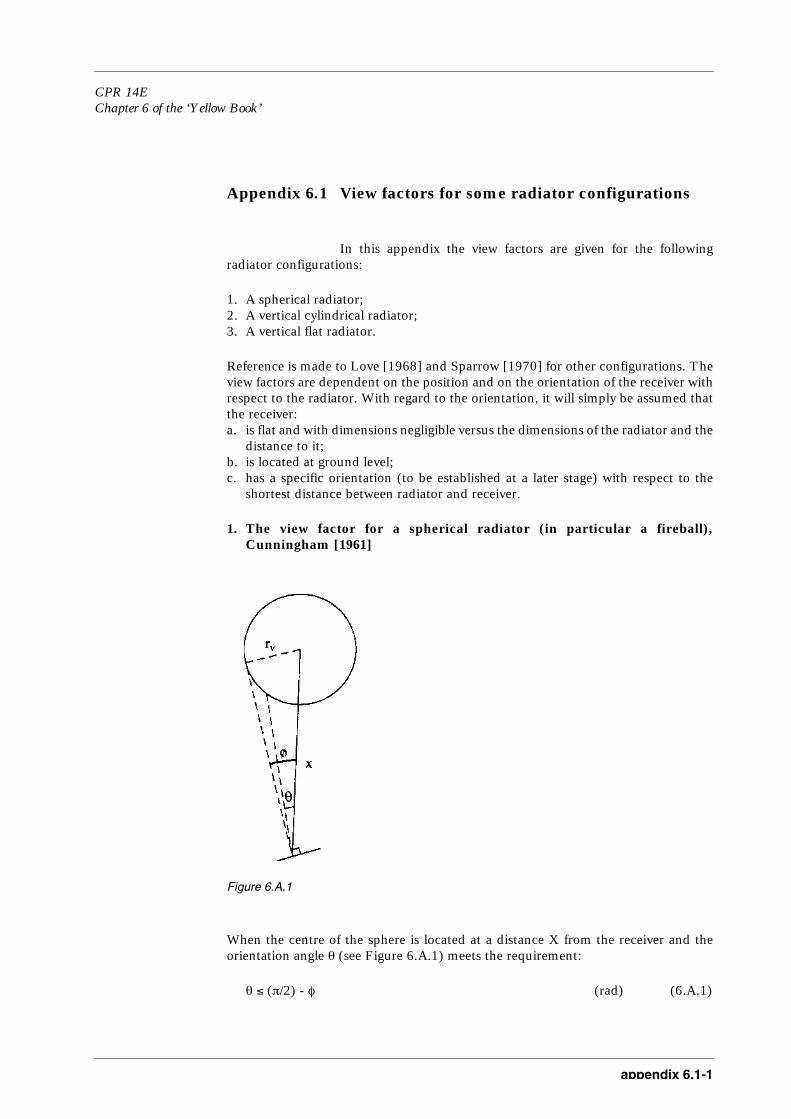
appendix 6.1-1
CPR 14EChapter 6 of the ‘Yellow Book’
Appendix 6.1 View factors for some radiator configurations
In this appendix the view factors are given for the followingradiator configurations:
1. A spherical radiator; 2. A vertical cylindrical radiator; 3. A vertical flat radiator.
Reference is made to Love [1968] and Sparrow [1970] for other configurations. Theview factors are dependent on the position and on the orientation of the receiver withrespect to the radiator. With regard to the orientation, it will simply be assumed thatthe receiver: a. is flat and with dimensions negligible versus the dimensions of the radiator and the
distance to it; b. is located at ground level; c. has a specific orientation (to be established at a later stage) with respect to the
shortest distance between radiator and receiver.
1. The view factor for a spherical radiator (in particular a fireball),Cunningham [1961]
Figure 6.A.1
When the centre of the sphere is located at a distance X from the receiver and theorientation angle θ (see Figure 6.A.1) meets the requirement:
θ ≤ (π/2) - φ (rad) (6.A.1)

appendix 6.1-2
in which φ is half the view angle, the view factor is simply given by:
Fview = (rfb/X)2 × cos θ (-) (6.A.2)
The sphere, in this case, is completely visible.
When the orientation angle is so wide that the sphere is not completely visible, whichis the case if:
θ > π/2 - φ (Rad) (6.A.3)
the view factor is then given by:
(6.A.4)
in which:
xr = X/rfb (-) (6.A.5)
In Figure 6.A.2 the view factors, in accordance to (6.A.4) are given for someorientation angles θ.
Figure 6.A.2 View factors for a spherical radiator as function of the ratio distance/radius (incomplete view)
Fview1
2--
1
π---– sin 1–
xr2 1–( )1/2
xr sin θ----------------------
1
πxr2
-------- cos θ cos 1– xr2 1–( )– 1/2 cot θ[ ]+=
1
πxr2-------- xr
2 1–( )1/2 1 xr2 cos2 θ–( )1/2–
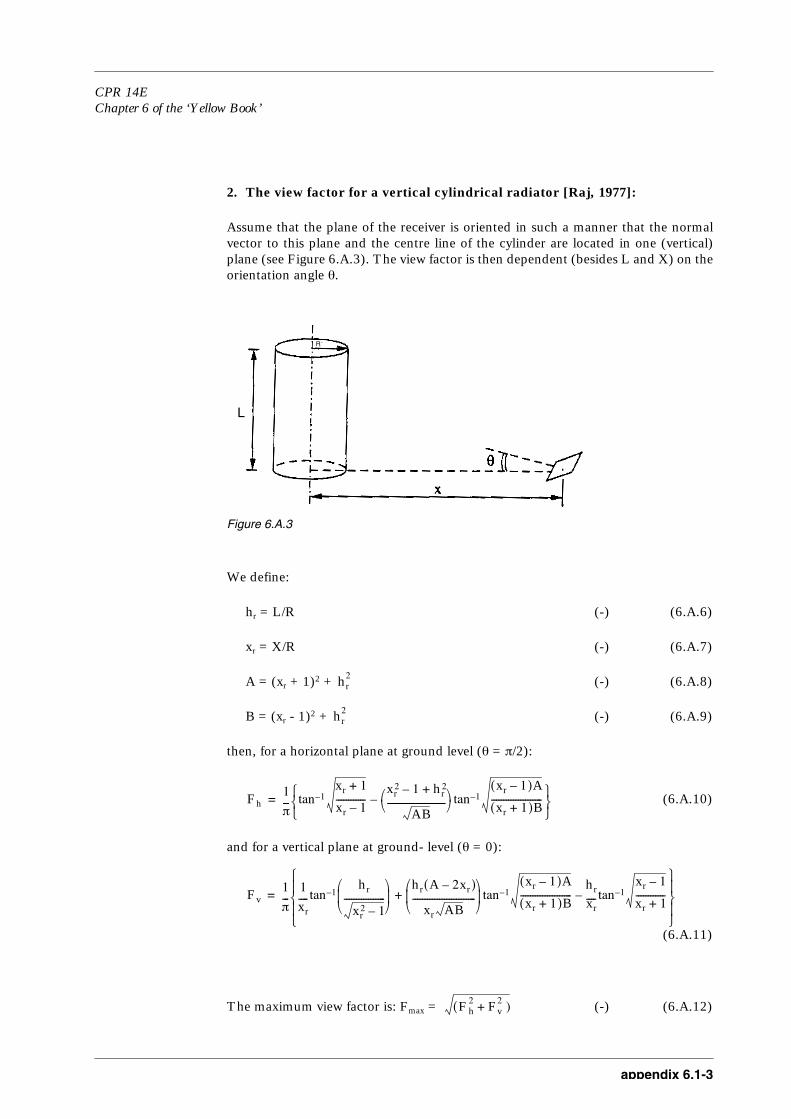
appendix 6.1-3
CPR 14EChapter 6 of the ‘Yellow Book’
2. The view factor for a vertical cylindrical radiator [Raj, 1977]:
Assume that the plane of the receiver is oriented in such a manner that the normalvector to this plane and the centre line of the cylinder are located in one (vertical)plane (see Figure 6.A.3). The view factor is then dependent (besides L and X) on theorientation angle θ.
Figure 6.A.3
We define:
hr = L/R (-) (6.A.6)
xr = X/R (-) (6.A.7)
A = (xr + 1)2 + (-) (6.A.8)
B = (xr - 1)2 + (-) (6.A.9)
then, for a horizontal plane at ground level (θ = π/2):
(6.A.10)
and for a vertical plane at ground- level (θ = 0):
(6.A.11)
The maximum view factor is: Fmax = (-) (6.A.12)
L
R
hr2
hr2
Fh1
π--- tan 1–
xr 1+
xr 1–------------
xr2 1– hr
2+
AB------------------------ tan 1––
xr 1–( )A
xr 1+( )B---------------------
=
Fv1
π---
1
xr----tan 1–
hr
xr2 1–
----------------- hr A 2xr–( )
xr AB--------------------------
tan 1–xr 1–( )A
xr 1+( )B---------------------
hr
xr----tan 1–
xr 1–
xr 1+------------–+
=
F( h2 Fv
2 )+
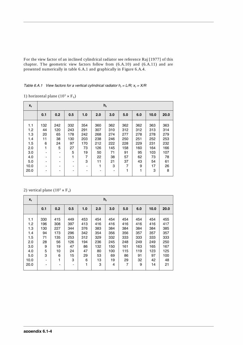
appendix 6.1-4
For the view factor of an inclined cylindrical radiator see reference Raj [1977] of thischapter. The geometric view factors follow from (6.A.10) and (6.A.11) and arepresented numerically in table 6.A.1 and graphically in Figure 6.A.4.
Table 6.A.1 View factors for a vertical cylindrical radiator hr = L/R; xr = X/R
1) horizontal plane (103 × Fh)
2) vertical plane (103 × Fv)
xr hr
0.1 0.2 0.5 1.0 2.0 3.0 5.0 6.0 10.0 20.0
1.11.21.31.41.52.03.04.05.0
10.020.0
13244201161-----
2421206538245-----
332243178130972751---
354291242203170731973--
3603072682382121265022111-
3623102742462221457138213-
36231227725022815891573771
36231227825122916095624391
3633132782522311641037354173
3633142792532321661077861268
xr hr
0.1 0.2 0.5 1.0 2.0 3.0 5.0 6.0 10.0 20.0
1.11.21.31.41.52.03.04.05.0
10.020.0
330196130947128953--
41530822717313556191061-
4493973442962531264724153-
45341337634231219486472961
4544163833543292361328053133
45441638435633224515010069194
45441638435633324816111586297
45441638435733324916311991329
454416384357333249165123974214
4554173853573332501671251004821
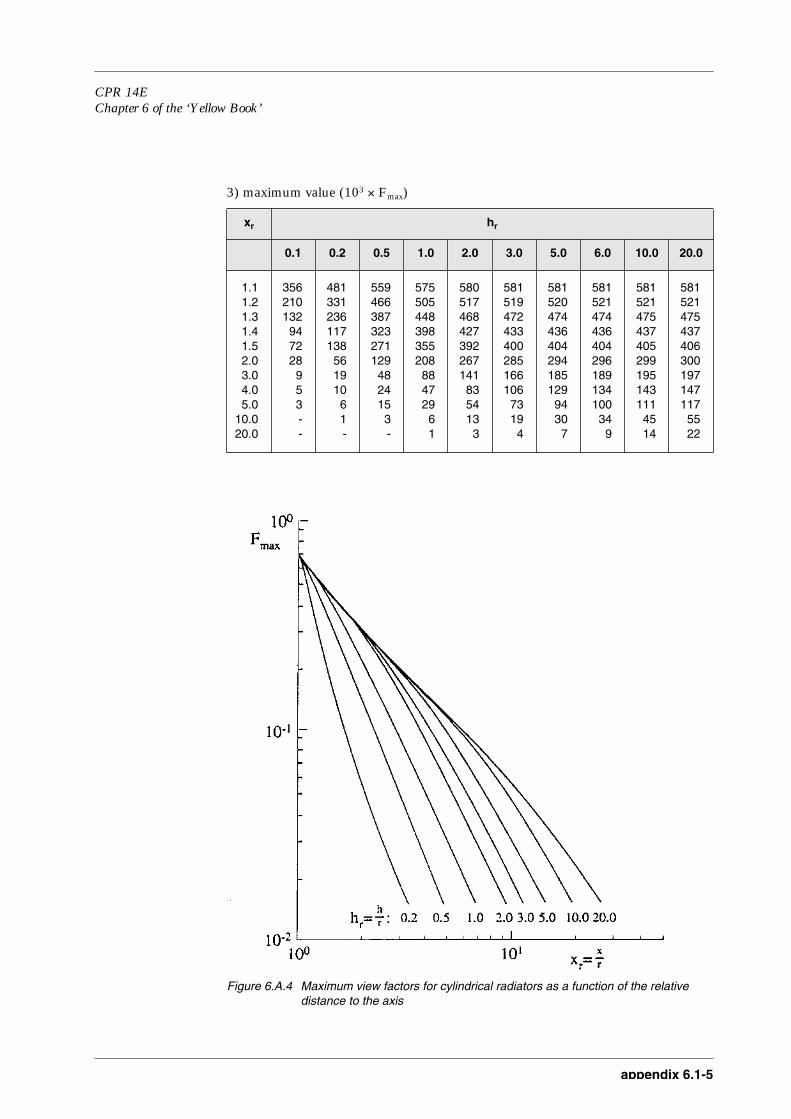
appendix 6.1-5
CPR 14EChapter 6 of the ‘Yellow Book’
3) maximum value (103 × Fmax)
Figure 6.A.4 Maximum view factors for cylindrical radiators as a function of the relative distance to the axis
xr hr
0.1 0.2 0.5 1.0 2.0 3.0 5.0 6.0 10.0 20.0
1.11.21.31.41.52.03.04.05.0
10.020.0
356210132947228953--
48133123611713856191061-
5594663873232711294824153-
57550544839835520888472961
5805174684273922671418354133
58151947243340028516610673194
58152047443640429418512994307
581521474436404296189134100349
5815214754374052991951431114514
5815214754374063001971471175522
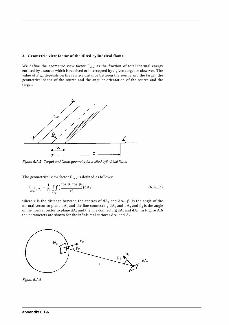
appendix 6.1-6
3. Geometric view factor of the tilted cylindrical flame
We define the geometric view factor Fview as the fraction of total thermal energyemitted by a source which is received or intercepted by a given target or observer. Thevalue of Fview depends on the relative distance between the source and the target, thegeometrical shape of the source and the angular orientation of the source and thetarget.
Figure 6.A.5 Target and flame geometry for a tilted cylindrical flame
The geometrical view factor Fview is defined as follows:
(6.A.13)
where x is the distance between the centres of dA1 and dA2, β1 is the angle of thenormal vector to plane dA1 and the line connecting dA1 and dA2 and β2 is the angleof the normal vector to plane dA2 and the line connecting dA1 and dA2. In Figure A.6the parameters are shown for the infinisimal surfaces dA1 and A2.
Figure 6.A.6
FdA1 A2,1π---
∫ β1 β2coscos
x2------------------------------- A2d∫=
view A2
x
n2
β2
β1
n1
dA1
dA2

appendix 6.1-7
CPR 14EChapter 6 of the ‘Yellow Book’
Mudan [1987] derived analytical geometrical view factor expressions for horizontaland vertical receiving targets for simple fire geometries including cylinder andrectangular parallelepiped.
3.1 Cylindrical flames
Consider a cylindrical approximation to the tilted flame as shown by Figure 6.A.5.The vertical and horizontal area view factors are given by the following expressions(also see Atallah [1990]):
a = L/R (Lb/R or Lf/R) (-)
b = X/R (-)
A = (-)
B =
C = (-)
D = (-)
E = (a × cos θ)/(b - a × sin θ) (-)
F = (-)
Lf is the tilted flame length. The angle of tilt θ is measured with respect to the verticaland is positive for targets located downwind from the source and negative for targetslocated upwind from the source.Additional forms are derived from calculating the view factors for a target in thecrosswind direction, i.e. whose direction is perpendicular to the tilt angle:
(6.A.14)
πFv E tan 1– D– E a2 b 1+( )2 2b 1 a sin θ+( )–+
AB--------------------------------------------------------------------- tan 1 – AD
B-------- +=
cos θ
C------------ tan 1–
ab F2 sin θ–
FC------------------------------ tan 1–
F2 sin θ
FC------------------ ++
6.A.15)
πFh tan 1– 1
D---- sin θ
C---------- tan 1–
ab F2 sin θ–
FC------------------------------ tan 1 – F2 sin θ
FC------------------ ++=
a2 b 1+( )2 2 b 1 ab sin θ+ +( )–+
AB----------------------------------------------------------------------------- tan 1–
AD
B--------
a2 b 1+( )2 2 a b 1+( ) θsin×××–+( )
a2 b 1–( )2 2 a b 1–( ) θsin×××–+( )
1 b2 1–( ) cos2θ×+( )
b 1–( )/ b 1+( )( )
b2 1–( )

appendix 6.1-8
where
G = (-)
H = a2 + (b + 1)2 (-)
I = (-)
The maximum view factor is estimated from the vector sum of Fh and Fv:
Fmax = (-) (6.A.18)
With minor modifications, Equations (6.A.14) and (6.A.15) can be used to estimatethe view factors when the flame base is elevated with respect to the target as shown inFigure 6.A.7, when the target is elevated with respect to the flame base as shown inFigure 6.A.8 and when the target is in the shadow of the flame as shown inFigure 6.A.9.
2πFh 2tan 1– D=
+F sin θ
I---------------- tan 1–
ab
F------ sin θ+
I-----------------------
tan 1–
ab
F------ sin – θ
I--------------------
2tan 1–– sin θ
I---------- –
(6.A.16)a2 b2 1–+
G------------------------ – tan 1–
HD 2a sin θ–
G------------------------------- tan 1– HD 2a sin θ+
G---------------------------------- +
(6.A.17)
2πFva2 sin θ cos θ
2 a2 sin2 θ b2+( )--------------------------------------
a2 b2 1– 2a Fb--- sin θ–+
a2 b2 1 2aFb---
sin θ+–+------------------------------------------------------ln–=
+ cos θ
I----------- tan 1–
ab
F------ sin θ+
I-----------------------
tan 1–+
ab
F------ sin – θ
I--------------------
+ ab cos θ
b2 a2 sin2 θ+-------------------------------
a2 b2 1+ +
G------------------------ tan 1–
HD 2a sin θ–
G--------------------------------- tan 1– HD 2a sin θ+
G--------------------------------- +
2ab cos θ
b2 a2 sin2 θ+------------------------------ – tan 1– D
a2 b2 1+ +( )(2
4 b2 a2 sin2θ×+( ) )×–
b2 sin2θ–( )
F( v2 Fh
2 )+

appendix 6.1-9
CPR 14EChapter 6 of the ‘Yellow Book’
Figure 6.A.7 Elevated flame with respect to target
Figure 6.A.8 Elevated target with respect to flame
Figure 6.A.9 Target in flame shadow
For an elevated flame base we modify the flame length and the target location:
x1 = X + z × tan θ (m) (6.A.19)

appendix 6.1-10
L1 = z/cos θ (m) (6.A.20)
L2 = L + L1 (m) (6.A.21)
The view factors are then calculated as follows:
Fv = Fv(L2) - Fv(L1) (-) (6.A.22)
Fh = Fh(L2) - Fh(L1) (-) (6.A.23)
The view factors are calculated in a similar fashion when the target is elevated withrespect to the flame base:
x1 = X - z × tan θ (m) (6.A.24)
L1 = z/cos θ (m) (6.A.25)
L2 = L - L1 (m) (6.A.26)
When the observer is in the flame shadow, the vertical view factor must be calculatedwith a truncated flame length:
L1 = X/sin θ (m) (6.A.27)
The horizontal view factor is unchanged.
4. The view factor for a vertical flat radiator, Raj [1977], Love [1968],Sparrow [1970]
It will be assumed here that the crossing lines of, respectively, the radiator with theground and the receiver with the ground, are parallel. The view factor will thenbe calculated as the sum of the factors for plane part I and plane part II (seeFigure 6.A.10). For each of these parts the following is defined:
Figure 6.A.10
L

appendix 6.1-11
CPR 14EChapter 6 of the ‘Yellow Book’
hr = L/b (-) (6.A.28)
xr = X/b (-) (6.A.29)
A = 1/ (-) (6.A.30)
B = hr/ (-) (6.A.31)
We have for horizontal plane at ground level (θ = π/2):
(6.A.32)
For a vertical plane at ground level (θ = 0):
(6.A.33)
The maximum view factor is given by:
Fmax = (-) (6.A.34)
It should be noted (except if bI = bII) that this is not the maximum view factor of aplane at a distance X from the radiator; this because of the restriction which is madewith respect to the orientation of the receiver. The view factors Fh, Fv and Fmax of theradiator can now be obtained simply by adding the values for plane part I and planepart II. Numerical values are given in table 6.A.2, and, Fmax versus xr is representedgraphically in Figure 6.A.10.
h( r2 xr
2 )+
1 xr2+
Fh1
2π------= tan 1– 1
xr---- A xrtan 1– A–
Fv1
2π------= hrA tan 1– A B
hr---- tan 1– B+
F( h2 Fv
2 )+
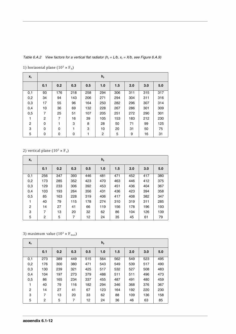
appendix 6.1-12
Table 6.A.2 View factors for a vertical flat radiator (hr = L/b, xr = X/b, see Figure 6.A.9)
1) horizontal plane (103 × Fh)
2) vertical plane (103 × Fv)
3) maximum value (103 × Fmax)
xr hr
0.1 0.2 0.3 0.5 1.0 1.5 2.0 3.0 5.0
0,1 93 176 218 258 294 306 311 315 3170,2 34 94 143 206 271 294 304 311 3160,3 17 55 96 164 250 282 296 307 3140,4 10 36 69 132 228 267 286 301 3090,5 7 25 51 107 205 251 272 290 3011 2 7 16 39 105 153 183 212 2302 0 1 3 8 28 50 71 99 1253 0 0 1 3 10 20 31 50 755 0 0 0 1 2 5 9 16 31
xr hr
0.1 0.2 0.3 0.5 1.0 1.5 2.0 3.0 5.0
0,1 256 347 393 446 481 471 452 417 3800,2 173 285 352 423 470 463 446 412 3750,3 129 233 306 392 453 451 436 404 3670,4 103 193 264 356 431 436 423 394 3580,5 85 163 228 319 406 417 408 382 3471 40 79 115 178 274 310 319 311 2852 14 27 41 66 119 156 178 196 1933 7 13 20 32 62 86 104 126 1395 2 5 7 12 24 35 45 61 79
xr hr
0.1 0.2 0.3 0.5 1.0 1.5 2.0 3.0 5.0
0,1 273 389 449 515 564 562 549 523 4950,2 176 300 380 471 543 549 539 517 4900,3 130 239 321 425 517 532 527 508 4830,4 104 197 273 379 488 511 511 496 4730,5 86 165 234 337 455 487 491 480 4591 40 79 116 182 294 346 368 376 3672 14 27 41 67 123 164 192 220 2303 7 13 20 33 62 88 109 136 1585 2 5 7 12 24 36 46 63 85

appendix 6.1-13
CPR 14EChapter 6 of the ‘Yellow Book’
Figure 6.A.11 Maximum view factors of flat radiators as a function of the relative distance to the radiator
Maximum view factors of flat radiators as a function of the relative distance to the radiator
1,0E+01
1,0E+02
1,0E+03
1,0E-01 1,0E+00 1,0E+01Xr
Fmax
hr=0,1
hr=0,2
hr=0,3
hr=0,5
hr=1
hr=2
hr=5
7 1
Chapter 7Rupture of vesselsJ.C.A.M. van Doormaal, R.M.M. van Wees

CPR 14EChapter 7 of the ‘Yellow Book’
7.3
Modifications to Chapter 7 (Rupture of Vessels)with respect to the first print (1997)
Numerous modifications were made concerning typographical errors. A list is givenbelow for the pages on which errors have been corrected.
In the section on initial fragment velocity calculations a scaled velocity correctionfactor graph is added.
Correction of Formula 7.19
Application of selected methods: calculation examplesA lot of numbers are refined, for example the ambient pressure of 0.1*106 is replacedby 1.01325*105, and values are more accurately read from plots and figures.
A large adjustment is made in step 12 in the calculation examples, in the 3rd editionit was accounted for that the vessel was slightly elevated using values of table 7.4, inthe fourth edition this has been removed.

7.4

CPR 14EChapter 7 of the ‘Yellow Book’
7.5
List of symbols of chapter 7
aa speed of sound in ambient air (7.9) m/sal speed of sound in compressed gas
(section 7.5.3, step 3b1) m/sAD exposed area in plane perpendicular to
trajectory (7.22) m2
AL exposed area in plane parallel to trajectory (7.22) m2
Aplate area of plate-like fragment (Table 7.8) m2
Asb constant for surface burst (7.7) -Ake fraction of available energy that goes into
kinetic energy of the fragments (7.15) -AM constant for Moore’s method (7.19) -CD drag coefficient (7.22) -CL lift coefficient (7.22) -dv vessel diameter (section 7.5.3, step 3b3) meav specific liberated energy (7.4) J/kgEav liberated or available energy (7.1) JEex explosion energy or blast wave energy (7.7) Jg acceleration of gravity (7.22) m/s2
h specific enthalpy (enthalpy per unit mass) (7.2) J/kg
h1 specific enthalpy in initial state (= at failure) (section 7.5.2, step 4b) J/kg
h2 specific enthalpy in final state(section 7.5.2, step 4c) J/kg
hf specific enthalpy of saturated liquid (7.3) J/kghg specific enthalpy of saturated vapour (7.3) J/kgis positive impulse of blast wave (7.14) Pa.sI non-dimensional impulse of blast wave (7.14) -Lv vessel length (section 7.5.3, step 3b3) mMv mass of empty vessel (7.15) kgMc total mass of vessel contents (7.6) kgMfl mass of released phase or component of the fluid
(7.5) kgMcap mass of end cap of cylindrical vessel
(Table 7.6) kgMf fragment mass (Table 7.6) kgnf number of fragments (section 7.5.3, step 2) -p absolute pressure (7.2) Papa ambient pressure (7.1) Pap1 vessel’s internal pressure (absolute) at
failure (7.1) PaP1 scaled pressure (7.16) -ps peak side-on pressure (absolute) of blast wave
(7.13) Papso peak shock pressure directly after burst
(7.12) Pa
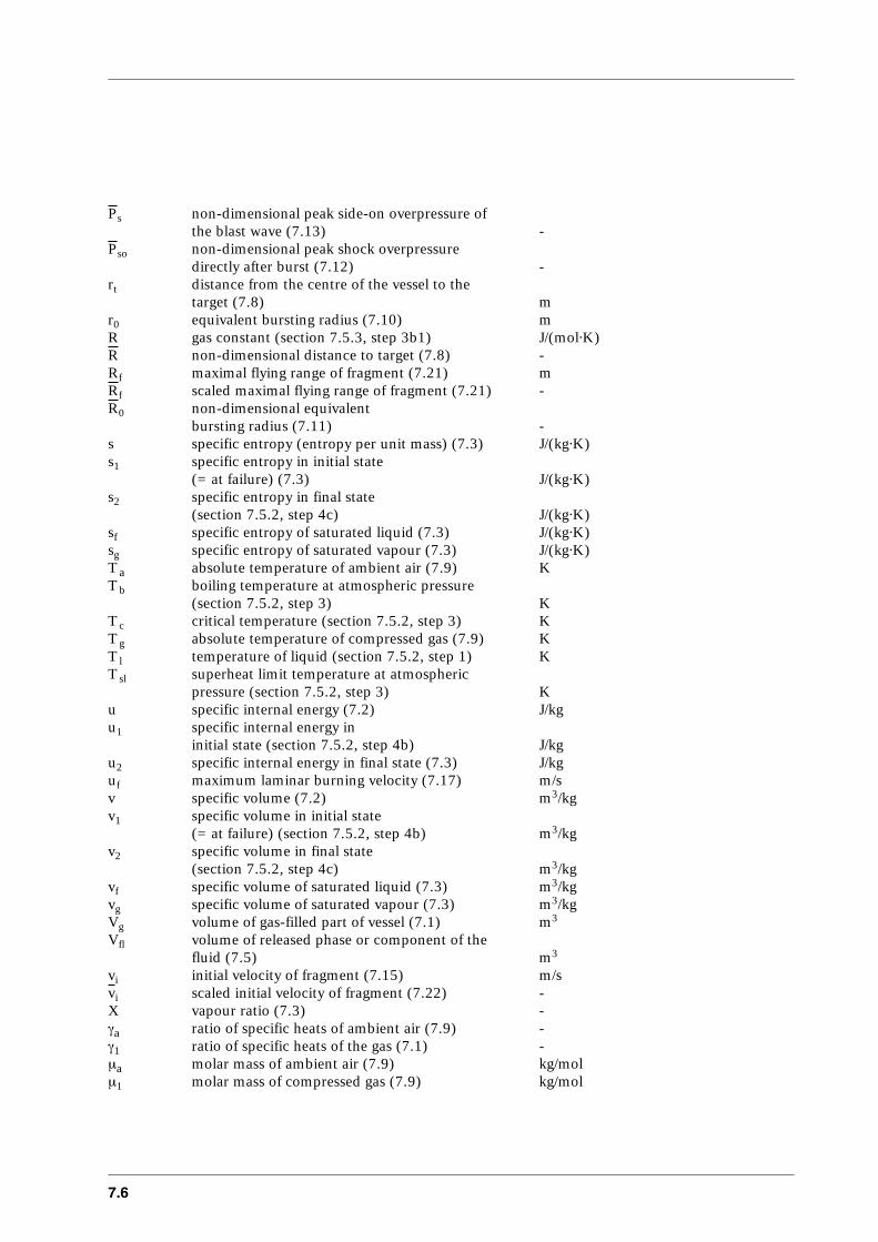
7.6
Ps non-dimensional peak side-on overpressure of the blast wave (7.13) -
Pso non-dimensional peak shock overpressure directly after burst (7.12) -
rt distance from the centre of the vessel to the target (7.8) m
r0 equivalent bursting radius (7.10) mR gas constant (section 7.5.3, step 3b1) J/(mol⋅K)R non-dimensional distance to target (7.8) -Rf maximal flying range of fragment (7.21) mRf scaled maximal flying range of fragment (7.21) -R0 non-dimensional equivalent
bursting radius (7.11) -s specific entropy (entropy per unit mass) (7.3) J/(kg⋅K)s1 specific entropy in initial state
(= at failure) (7.3) J/(kg⋅K)s2 specific entropy in final state
(section 7.5.2, step 4c) J/(kg⋅K)sf specific entropy of saturated liquid (7.3) J/(kg⋅K)sg specific entropy of saturated vapour (7.3) J/(kg⋅K)Ta absolute temperature of ambient air (7.9) KTb boiling temperature at atmospheric pressure
(section 7.5.2, step 3) KTc critical temperature (section 7.5.2, step 3) KTg absolute temperature of compressed gas (7.9) KTl temperature of liquid (section 7.5.2, step 1) KTsl superheat limit temperature at atmospheric
pressure (section 7.5.2, step 3) Ku specific internal energy (7.2) J/kgu1 specific internal energy in
initial state (section 7.5.2, step 4b) J/kgu2 specific internal energy in final state (7.3) J/kguf maximum laminar burning velocity (7.17) m/sv specific volume (7.2) m3/kgv1 specific volume in initial state
(= at failure) (section 7.5.2, step 4b) m3/kgv2 specific volume in final state
(section 7.5.2, step 4c) m3/kgvf specific volume of saturated liquid (7.3) m3/kgvg specific volume of saturated vapour (7.3) m3/kgVg volume of gas-filled part of vessel (7.1) m3
Vfl volume of released phase or component of the fluid (7.5) m3
vi initial velocity of fragment (7.15) m/svi scaled initial velocity of fragment (7.22) -X vapour ratio (7.3) -γa ratio of specific heats of ambient air (7.9) -γ1 ratio of specific heats of the gas (7.1) -µa molar mass of ambient air (7.9) kg/molµ1 molar mass of compressed gas (7.9) kg/mol

CPR 14EChapter 7 of the ‘Yellow Book’
7.7
Φ dimensionless parameter that characterises theenergy release (7.17) -
ρa density of ambient air (7.21) kg/m3
∆Hf heat of reaction per kg product (7.6) J/kg
Note: the numbers betwen brackets refer to equations.

7.8
CPR 14EChapter 7 of the ‘Yellow Book’
7.9
Glossary of terms
blast Rapidly propagating pressure or shock wave inatmosphere with high pressure, high density andhigh particle velocity.
BLEVE Boiling Liquid Expanding Vapour Explosion: Atvessel rupture the liquefied contents of the vesselboil and flash instantaneously, causing aconsiderable blast. When the contents areflammable a large fireball can be formed.
explosion A sudden release of energy that causes a blast.
fragment range Distance a fragment can fly.
impulse A measure used to quantify the consequences ofa short duration pressure pulse. It is calculatedby the integration of the pressure-time curve.
pressure vessel burst Vessel burst of a pressurised container (notnecessarily a true pressure vessel).
pressure wave Rapidly propagating wave in atmosphere causinga gradual change in gas-dynamic-state: highpressure, high density and high particle velocity.
primary effects Effects that occur in the first instance and thatoriginate from the source itself: blast wave,fragments of vessel.
secondary effects Effects that occur in the second instance and/orthat originate from other sources: e.g. fireball,debris picked up by blast wave.
shock wave Rapidly propagating wave in atmosphere causingan instantaneous change in gas-dynamic-state:high pressure, high density and high particlevelocity.
side-on pressure or impulse The pressure or impulse experienced by anobject as a blast wave passes by.

7.10
CPR 14EChapter 7 of the ‘Yellow Book’
7.11
Table of contents of chapter 7
Modifications to Chapter 7, Rupture of Vessels ...................................3
List of symbols of chapter 7 ...................................................................5
Glossary of terms ...................................................................................9
7 Rupture of vessels ................................................................................137.1 Introduction..................................................................................137.2 The phenomenon of vessel rupture ................................................15
7.2.1 Effects.................................................................................157.2.2 Causes of vessel ruptures .....................................................167.2.3 Types of bursts....................................................................17
7.3 General overview of existing methods.............................................197.3.1 Introduction to section 7.3...................................................197.3.2 Methods for blast effects ......................................................197.3.3 Methods for fragmentation effects ........................................21
7.4 Selection of methods .....................................................................257.4.1 Introduction to section 7.4...................................................257.4.2 Methods for blast effects ......................................................257.4.3 Methods for fragment velocity and range ..............................26
7.5 Description of selected methods.....................................................277.5.1 Introduction to section 7.5...................................................277.5.2 Methods for calculating the blast effects ...............................277.5.3 Methods for fragmentation effects ........................................44
7.6 Application of selected methods: calculation examples ....................597.6.1 Introduction to section 7.6...................................................597.6.2 Example 1: blast effects .......................................................597.6.3 Example 2: fragments ..........................................................69
7.7 Interfacing with other models ........................................................737.8 Discussion ....................................................................................757.9 Literature......................................................................................77

7.12

CPR 14EChapter 7 of the ‘Yellow Book’
7.13
7 Rupture of vessels
7.1 Introduction
A vessel rupture is coupled with the release of the contents and the releaseof the internal energy. Depending on the characteristics of the material in the vessel,the released contents can cause a buoyant fireball, a vapour cloud explosion, a flashfire or toxic gases. The sudden release of energy can give rise to damaging blast wavesand high velocity fragments.This chapter presents methods that enable the prediction of the blast waves, vesselfragmentation and fragment velocities. The other effects mentioned are treated inother chapters, see section 7.7.
A basic understanding of the phenomena of vessel burst is necessary before one canstart with any calculations. One must be able to identify the problem underconsideration. All types of vessel bursts can be divided into five categories: pressurevessel bursts with non-reactive contents, BLEVEs, runaway reactions, decompositionof energetic materials and internal explosions. For each category the approach tocalculate the effects is different.Section 7.2 provides the essential and basic understanding of the phenomena.Anyone who is not familiar with the subject is advised to start by reading this section.
Section 7.3 provides a general overview of the currently available methods for aquantified analysis. It includes some background to the methods. The aim of thesection is also to position the methods selected for detailed description among otherexisting methods.
Section 7.4 presents the considerations which led to the selection of methodsdescribed in this chapter.
Section 7.5 provides the detailed and complete description of the selected methods.
Section 7.6 presents examples of the use of the methods presented in section 7.5.
Section 7.7 directs the user to other chapters for effects of vessel rupture other thanblast waves and fragmentation.
Finally section 7.8 provides some information on general restrictions regardingapplication of the methods.

7.14

CPR 14EChapter 7 of the ‘Yellow Book’
7.15
7.2 The phenomenon of vessel rupture
7.2.1 Effects
A vessel can rupture due to several causes, but in all situations the effectsare similar. Vessel rupture produces three primary effects:1. release of vessel contents,2. fragmentation of the vessel coupled with missile effects, and3. blast due to the expansion of the pressurised contents.
The release of the vessel contents can cause so-called secondary effects, such as abuoyant fireball with heat radiation, a vapour cloud explosion, a flash fire ordispersion of a toxic substance. Whether these secondary effects will occur dependsamong others on the flammability and toxicity of the contents. The above-mentionedsecondary effects are the subject of other chapters and hence not considered here.The fragments of the vessel can become missiles with high velocities that will bepropelled for a long distance and that will hit anything they find on their way. Theinternal energy of the vessel’s contents is partly converted into kinetic energy of thefragments.Another part of the internal energy is converted into expansion of the contents of thevessel. This form of mechanical energy is transmitted to the surrounding atmospherein the form of a blast wave.In the surrounding atmosphere, a blast wave is experienced as a transient change ingas-dynamic-state parameters: pressure, density and particle velocity. This meansthat a blast wave has the potential to crush objects due to the overpressure or to blowthem over due to wind force. Generally the parameters increase rapidly orinstantaneously after which they decrease gradually to sub-ambient values, i.e. anegative phase is developed. Subsequently, the parameters slowly return toatmospheric values. Rapid and slow are relative terms here. Generally, a blast wavelasts a fraction of a second.Figure 7.1 shows two examples of very common shapes of a blast wave. The shapehighly depends on the nature of the expansion process. In case of a slow expansionprocess, the blast consists of a low-amplitude pressure wave that is characterised by agradual increase in pressure (Figure 7.1a). If, on the other hand, expansion is rapid,the blast is characterised by a steep increase, the so-called shock (Figure 7.1b). Themost important shock wave parameters are the peak overpressure ps and the positiveimpulse is, which is calculated by integration of the pressure-time curve.
Figure 7.1 Blast wave shapes
a) b)
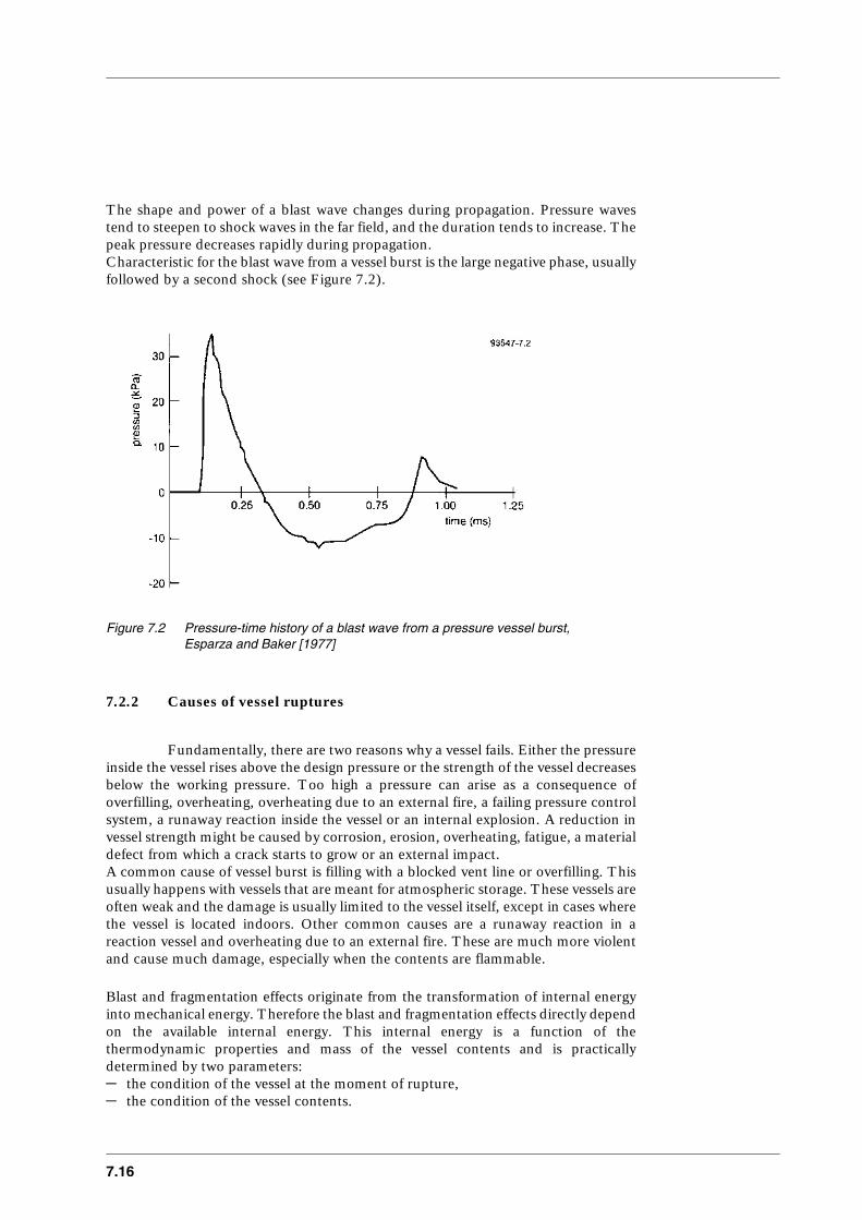
7.16
The shape and power of a blast wave changes during propagation. Pressure wavestend to steepen to shock waves in the far field, and the duration tends to increase. Thepeak pressure decreases rapidly during propagation.Characteristic for the blast wave from a vessel burst is the large negative phase, usuallyfollowed by a second shock (see Figure 7.2).
Figure 7.2 Pressure-time history of a blast wave from a pressure vessel burst,Esparza and Baker [1977]
7.2.2 Causes of vessel ruptures
Fundamentally, there are two reasons why a vessel fails. Either the pressureinside the vessel rises above the design pressure or the strength of the vessel decreasesbelow the working pressure. Too high a pressure can arise as a consequence ofoverfilling, overheating, overheating due to an external fire, a failing pressure controlsystem, a runaway reaction inside the vessel or an internal explosion. A reduction invessel strength might be caused by corrosion, erosion, overheating, fatigue, a materialdefect from which a crack starts to grow or an external impact.A common cause of vessel burst is filling with a blocked vent line or overfilling. Thisusually happens with vessels that are meant for atmospheric storage. These vessels areoften weak and the damage is usually limited to the vessel itself, except in cases wherethe vessel is located indoors. Other common causes are a runaway reaction in areaction vessel and overheating due to an external fire. These are much more violentand cause much damage, especially when the contents are flammable.
Blast and fragmentation effects originate from the transformation of internal energyinto mechanical energy. Therefore the blast and fragmentation effects directly dependon the available internal energy. This internal energy is a function of thethermodynamic properties and mass of the vessel contents and is practicallydetermined by two parameters:– the condition of the vessel at the moment of rupture,– the condition of the vessel contents.

CPR 14EChapter 7 of the ‘Yellow Book’
7.17
The condition of vessel and contents relate to the cause of container failure. In caseof a fire near/below vessels filled with pressurised liquefied gases for instance, directflame impingement will weaken the container walls. The pressure at which thecontainer fails will usually be about equal to the pressure at which the safety valveoperates. The temperature of the contents will usually be considerably higher than theambient temperature.If a vessel ruptures as a result of excessive internal pressure, its bursting overpressuremay be several times higher than its design overpressure. However, if the rupture isdue to corrosion or mechanical impact, bursting pressure is approximately equal tothe working pressure. The temperature in these situations will depend on processconditions.
7.2.3 Types of bursts
The calculation of blast and fragmentation effects of vessel bursts canroughly be divided into two steps. In the first step the available energy is calculated,in the second step the effects are based on the energy resulting from the first step. Thissecond step is principally the same for all types of vessel bursts. In the first stephowever, distinction must be made between various types of vessel bursts. Differentmethods must be used for each way in which the internal energy can be liberated fortransformation into mechanical energy. In relation to the liberation of the internalenergy all types of vessel bursts can be subdivided into the following six groups:– pressure vessel bursts with ideal gas,– pressure vessel bursts with non-ideal gas or vapour,– BLEVEs,– (exothermic) runaway reaction,– decomposition of energetic materials,– internal explosion.
Pressure vessel bursts concern vessels containing a pressurised gas or vapour. Theonly source of energy for blast and fragmentation is the expansion of the gas orvapour. The liquid does not or only slowly flash, so that it will not supply a significantamount of energy. There is no fundamental difference in behaviour between vesselsfilled with ideal or non-ideal gases. Only the calculation methods that are to be usedfor the energy differ.
A BLEVE is an explosion resulting from the failure of a vessel containing a liquid ata temperature significantly above its boiling point at normal atmospheric pressure,e.g. pressure liquefied gases. The fluid in the vessel is usually a combination of liquidand vapour. Before rupture, the liquid contained is more or less in equilibrium withthe saturated vapour. If the vessel ruptures, vapour is vented and the pressure in theliquid drops sharply. Upon loss of equilibrium, liquid flashes at the liquid-vapourinterface, the liquid-container-wall interface, and, depending on temperature,throughout the liquid.Instantaneous boiling throughout the liquid will occur whenever the temperature ofthe liquid is higher than the superheat temperature (nucleation temperature).Microscopic vapour bubbles begin to form and grow, generally at submicronnucleation sites such as impurities, crystals or ions. Through this process, a largefraction of the liquid can vaporise within milliseconds. The liberated energy in suchcases is very high, causing high blast pressures and generation of fragments with high
7.18
initial velocities, and resulting in propulsion of fragments over long distances. Noboiling occurs if the temperature is below the boiling temperature. Between thesetemperatures, the liquid may boil instantaneously under certain conditions,Venart et al. [1992].
Runaway reactions can occur in a vessel if the heat of reaction or decompositionexceeds the cooling capacity of the vessel. The runaway itself is characterised by anexponential increase of temperature with time. The pressure increases due to theformation of non-condensable gases and/or an increasing vapour pressure of theliquid components. This process can only be controlled by a properly dimensionedpressure relief device, like a rupture disc or pressure relief valve. If these devicesmalfunction or if the reaction is faster than foreseen, the pressure may continue to riseuntil the vessel fails.
Materials can decompose so fast and release so much energy that a transition from arunaway reaction to a deflagration or even a detonation can occur. These materialsare called energetic materials. The contents of the vessel may decompose withinmilliseconds and the reaction of the entire contents may even be completed before thevessel bursts open. The explosions they cause are more like explosions from highexplosives than like pressure vessel bursts. In fact, many of these energetic materialscan also be made to detonate outside a vessel.
Internal explosions typically occur in storage or transport tanks when a flammablevapour-air or dust-air mixture is ignited, e.g. by a spark. This mixture burns in a fewtenths of a second. Since many of these explosions occur during filling or cleaning,they often cause no more than a jet fire through the opened hatch, but sometimes thevessel ruptures.
For the pressure vessel burst and the BLEVE, the vessel rupture can be due to anexcessive pressure or a weakening of the vessel. A runaway reaction and an internalexplosion on the other hand, are due to an excessive pressure. In these two situations,energy is not only released by the expansion of the contents of the vessel. Anadditional source of energy can be respectively the chemical reaction or thecombustion, which may continue after failure of the vessel.

CPR 14EChapter 7 of the ‘Yellow Book’
7.19
7.3 General overview of existing methods
7.3.1 Introduction to section 7.3
The scope of this section is to give an overview of the existing methods forpredicting the blast fragmentation effects of a vessel burst.Little research has been carried out to bursting vessels. The number of methods forcalculating the effects is therefore limited. Most of the research deals with pressurevessels with ideal gases. Just a few studies have been devoted to vessels filled with non-ideal gases and liquids. Little has been done in the field of vessel ruptures due to arunaway reaction or an internal explosion.
7.3.2 Methods for blast effects
Methods for calculating blast effects of pressure vessel bursts can roughlybe divided into two categories:1. Methods solving the set of differential equations of fluid mechanics by which the
shock wave can be described.2. Generalised methods based on thermodynamic terms and the available energy for
blast generation.
Methods to solve the equations of fluid mechanics
The differential equations that describe the shock wave are non-steady and non-linear. Numerical integration techniques are necessary to solve the equations unlessmany simplifications are allowed. With these simplifications it may be possible tosolve the equations analytically.
Analytical work is scarce. A valuable study is the analytical analysis of a burstingmembrane in a shock tube with a one-dimensional technique by Liepmann andRoshko [1967]. As a result of this analysis, a relationship for the initial overpressureat the shock front has been obtained, which is valid for all types of pressure vesselbursts. The initial overpressure depends on the pressure in the sphere, the speed ofsound and the ratio of specific heats. The equation of Liepmann and Roshko is animplicit equation which can be solved by iteration.
Many numerical methods have been proposed for solving the differential equationsand calculating the blast effects, most of them finite-difference methods. Most workin this area reported in open literature concerns ideal gas. See for instance Baker etal. [1977], Boyer et al. [1958], Huang and Chou [1968] and Guirao et al. [1979],who used several types of methods.Specialised commercial computer programs for numerical calculation of blast effectsfrom a vessel burst are not available. Some general purpose Eulerian-Lagrangiancodes, like Autodyn or MSC Pisces, may be used to predict blast and fragmentvelocities. Within these codes one has to set up the problem oneself. For that purposeone needs to have knowledge of the chosen code and also of vessel bursts.

7.20
Methods based on thermodynamics
In the second category of the generalised methods, based on thermodynamics, thedifferent states of the vessel contents before the start and after the completion of theexplosion process are compared. The explosion energy can thus be calculated. Thisexplosion energy is an appropriate quantity for comparing the vessel burst with well-known and well-defined explosions, so that the characteristics of the blast wave canbe estimated.
There are two methods that belong to this category. These are the TNT-equivalencemethod and a method developed by Baker et al. [1977].The TNT-equivalence method is often-used for blast calculations, since the blasteffects from TNT have been well studied and are well-known. Therefore, thisapproach gives the user access to a large body of blast field, blast-structure interactionand structural response data. Based on the available energy an equivalent amount ofTNT, for which the blast effects are known, can be calculated.One should be well aware of the fact that compared to a TNT-explosion, the shockwave produced by bursting vessels has lower initial overpressures, a slower decay ofthe overpressure with distance, longer positive phase durations, much larger negativephases and strong secondary shocks. Therefore, the TNT-equivalence method givesonly reasonable results for far range, which definition is related to the explosionenergy. Usually, one can speak of far range at a distance of 10 to 20 times the vesseldiameter or more.
Pressure vessel bursts
The method proposed by Baker et al. [1977] has been developed for pressure vesselbursts with an ideal gas and was later extended for vessels with non-ideal gases. Themethod differs from the TNT-equivalence method in the distinction between far andclose range for vessels. For far range, the method makes use of the similarity with highexplosives, in this case Pentolite. For close range, the method is based on results fromnumerical calculations on vessel bursts with an ideal gas. These numericalcalculations were verified by experiments. The close range modification is onlyapplicable to vessels with ideal gases.
In addition to the blast calculation method, Baker gives a simple correction methodfor including the influence of a nearby surface and a correction method for acylindrical vessel instead of a spherical one.The correction method for a nearby surface is based on experimental results with free-air explosions of a high explosive. It was not experimentally validated for pressurevessel bursts by Baker. Later Cain et al. [1992] showed the validity of the method witha limited number of tests. Other methods are not found in literature. The influenceof a nearby surface appeared to have received little attention. Pittmann [1976] didstudy the influence of a nearby surface using a two-dimensional code. His results,however, were inconclusive because of the small number of cases studied and thecoarse grid used in the code.The correction method for cylindrical vessels is based on knowledge of non-sphericalexplosions of high explosives and on qualitative knowledge of cylindrical vessel burstsonly. Although several researchers studied the effects of cylindrical vessel bursts, thisdid not result in methods for calculating the effects. Only qualitative knowledge has
CPR 14EChapter 7 of the ‘Yellow Book’
7.21
been gained, for instance that the shock wave along the axis of the vessel is initiallyconsiderably weaker than the wave normal to the axis.
BLEVEs
The work done in the field of BLEVEs is much more limited. Most studies onlyproduced qualitative knowledge about BLEVEs.There is the theoretical work of Reid [1976] and some experimental work by Venartet al. [1992], which increases the understanding of the phenomenon of a BLEVE andwhich gives a method to predict whether a BLEVE will occur or not, but the effectsof a BLEVE have not been considered. This theory is in most cases applicable.The only method for blast predictions for these situations is given by Baker et al.[1977]. Baker’s method includes a modification for vessels with flashing liquids,similar to the method for non-ideal gases.
Runaway reactions
Heemskerk [1995] conducted a study into the blast effects of runaway reactions. Heconcluded that reaction rates are too low to raise the pressure inside the vessel abovethe failure pressure during the failure process of the vessel. The energy of the ongoingreaction after the moment the vessel ruptures hardly contributes to the blast effects.For blast calculations a vessel burst due to a runaway reaction can therefore be treatedsimilar to a pressure vessel burst with ideal or non-ideal gases.
Internal explosions
The same is likely to be true for internal explosions, but this has not been studied. Aconservative approach is to assume that the combustion is complete and use Baker’smethod.
Decomposition of energetic materials
The decomposition of energetic materials is always approached with TNT-equivalency methods. A main point of discussion is the fraction of energy whichcontributes to the blast, because often a part of the contents of the vessel does notdecompose or decomposes too slowly to be able to fully contribute to the blast. Theresearch effort on energetic materials focuses on the question of explosiveness ofmaterials, Yoshida [1987], Heemskerk [1995]. This is outside the scope of thischapter.
7.3.3 Methods for fragmentation effects
The fragmentation of the vessel is coupled with missile effects. These so-called primary missile effects (= missiles that originate from the source itself) aredetermined by number, mass, shape, velocity and trajectory of the fragments.Secondary missiles, objects in the environment of the vessel that are picked up by theblast wave, are not considered.
7.22
Methods for calculating fragment velocity
The methods available for calculating the initial fragment velocity can be divided intothree groups:1. kinetic energy methods,2. methods based on theoretical considerations,3. empirical formulae.
The first group of methods is based on the assumption that a particular fraction of theenergy will be transferred into kinetic energy of the fragments. The differencebetween the various methods in this group lies in the difference in definition of thefragment energy. As for blast effects, it is not known which measure for the kineticenergy is most suitable. Some definitions prescribe all or almost all internal energy forthe calculation. It may be obvious that an upper limit will be found. Other definitionsprescribe a part of all internal energy, based on experimental observations. In casessimilar to the experiments these definitions may give a very good result. In other casesthey may over- or underestimate the kinetic energy.Theoretically, these methods are applicable to all types of vessel bursts, except tovessels filled with energetic materials, but it is not always simple to define the kineticenergy.
The second group of methods for estimating the fragment velocity is based ontheoretical considerations.A method for pressure vessels filled with ideal gas was introduced by Grodzovskii andKukanov [1965] and improved by various researchers. This method takes intoaccount gas flow through the ever-increasing gaps between fragments. Baker et al.[1983] used such a theoretical method to perform a parameter study and to composewith the results a diagram which can be used to determine initial fragment velocity forbursting pressurised vessels filled with ideal gas. The diagram is only applicable tospherical vessels or cylindrical vessels with a length-to-diameter ratio of 10, that havea uniform thickness and contain ideal gases. Furthermore, the diagram has beenobtained for vessels bursting into equal fragments. Therefore, one must be careful toapply the diagram for unequal fragments.
A second method belonging to the group of methods based on theoreticalconsiderations is given by Gel’fand et al. [1989]. Gel’fand et al. composed somedimensionless diagrams which can be used to determine the velocity of fragments inthe rupture of spherical and cylindrical vessels containing an inert or a reactive gasmixture. For the reactive mixture two situations are considered: a runaway reactionand a combustion.The diagrams are based upon a set of differential equations describing the motion ofthe fragments, the gas state, the energy of the mixture and the kinetics of the chemicalreaction. The flow of gas through gaps between the fragments is taken into account.The set has been solved by applying the Runge-Kutta numerical integration method.The method of Gel’fand is based on, first, the assumption that non-uniformdistribution of parameters with regard to the fragmentation effects may be ignoredand, secondly, on the assumption of isentropic flow. These assumptions are allowedin case of large fragments.Only the results for the inert mixture were compared with a limited number ofexperimental results and did correspond well. Gel’fand et al. state that the velocityestimate in case of a reactive mixture is conservative, whereas the velocity in case ofan inert mixture is underestimated by no more than 5%.
CPR 14EChapter 7 of the ‘Yellow Book’
7.23
The third group contains empirical relations for the initial velocity for vessels filledwith ideal gases. Moore [1967] presents an empirical relation which distinguishesspherical and cylindrical vessels. The relation is derived for fragments acceleratedfrom high explosives packed in a casing. Therefore, this equation predicts velocitieshigher than actual, especially for low vessel pressures and few fragments.Baum [1987] gives a set of empirical relations to calculate an upper value for theinitial fragment velocity from a spherical or cylindrical vessel burst, filled with an idealgas or a flashing liquid (BLEVEs), into a small or large number of fragments. Someof the equations are based on a very small number of experiments.
For internal explosions and runaway reactions, only Gel’fand et al. [1989] present amethod (see above).
The method of Gurney [Brown, 1985], and its adaptation by Moore (see above)could be considered for vessels filled with energetic materials. Gurney’s method wasderived for cased high explosives.
Methods to calculate fragment ranges
For the methods to calculate the fragment ranges (= flying distance), it is not requiredto distinguish between the four types of vessel bursts. The fragment range iscalculated given the initial velocity and the mass of the fragment.
The forces that act upon fragments during their flight are gravity and dynamic fluidforces. The latter can be subdivided into drag and lift components, i.e. friction anduplift.The simplest method to calculate the fragment range is by neglecting the dynamicfluid forces. Then the range only depends on the initial velocity and the initialtrajectory angle. With this method the fragment range is usually considerablyoverestimated, but when lift forces are high it can also be underestimated.
Baker et al. [1983] solved a set of differential equations for the fragment range whichincluded the fluid-dynamic forces by assuming that the orientation of a fragmentduring its flight remains the same with respect to its trajectory. They plotted theresults in a diagram for practical use. The curves were generated by maximisation ofrange through variation of the initial trajectory angle. The curves concern similar lift-to-drag ratios which are not always easy to determine, because these ratios vary withthe angle of attack and during the flight. A method to calculate the ratios is also given.
In some accidents rocketing effects are developed. Large fragments are propulsed forunexpectedly long distances. Baker et al. [1978] provided (1) equations for asimplified rocketing problem and (2) a computer program for a rocketing problem,but they stated that the method was not yet ready to be used for range prediction.Ranges for rocketing fragments can also be calculated from guide-lines by Baum[1987]. The difference between this approach and Baker’s approach appear to besmall.

7.24
Mass and range distributions of fragments
The methods presented previously give no information on distributions of mass,velocity and range of fragments, and no information on the number of fragments tobe expected. There are no methods that consider these parameters.Some information might be found in the analysis of results of accidental explosions.Vital information is, however, lacking for most of such events. A pragmatic approach,based on the small amount of information available, is proposed by us to overcomethis problem.Baker et al. [1978] analysed 25 accidental vessel explosions for mass and rangedistribution, number of fragments and fragment shape, divided into six groups of likeevents. With statistical analyses estimates of range distributions for the six groups andfragment-mass distributions for three of the six groups were obtained and plotted indiagrams. With these figures it is possible to estimate the percentage of all thefragments which would have a range or mass smaller than, or equal to, a certain value.This is only valid for cases exactly the same as studied. The quantitative informationcannot be generalised because of lacking data.
CPR 14EChapter 7 of the ‘Yellow Book’
7.25
7.4 Selection of methods
7.4.1 Introduction to section 7.4
In the field of vessel bursts sometimes only one method is available or evennone. When there are more methods, in this section the considerations will beexplained for the selection of the methods which will be included in section 7.5.In general the selection is based on the following criteria:1. The method should give accurate results.2. The method should be based on plausible physical assumptions.3. The method should be easy to apply, also for someone not familiar with the field.4. The method should preferably be widely applicable.5. The limits for the applicability of the method should be well defined.
The considerations will be presented as follows:1. Section 7.4.2 addresses the methods for predicting the blast effects.2. Section 7.4.3 addresses the methods for predicting the fragment velocity and other
fragmentation effects.
7.4.2 Methods for blast effects
For the description in section 7.5 a method based on thermodynamics hasbeen chosen. The limitation of methods of this category, that the energy available forblast is not well-known and that therefore the method is not very accurate, isoutreached by the simpleness of the method and its broad applicability. For thesereasons these methods have been used widely. No specialist knowledge of vesselbursts is necessary to use the method, the opposite of which is true when solving thedifferential equations of fluid mechanics. Moreover, although the blast energy is notwell-known, it is possible to define a conservative approach.
In this category there are only two methods which are more or less generallyapplicable. These two methods are:– TNT-equivalence method;– Baker’s method.
Both methods are comparable, except that Baker’s method distinguishes betweenclose and far range for pressure vessel bursts with ideal gas. For these scenariosBaker’s method is more accurate. Therefore, Baker’s method is described in section7.5.The method can be used for all six types of vessel bursts with a different definition forthe available energy for each type of burst.
7.26
7.4.3 Methods for fragment velocity and range
In section 7.5 the kinetic energy method is described because it provides avery simple method to obtain a rough estimate of the fragment velocity. The methodis always applicable, to each type of vessel burst and regardless of the number offragments.
Other, more accurate, methods are: (1) Baker’s method for rupture of vessels withinert gases into many fragments, (2) Baker’s and Gel’fand’s method for rupture ofvessels with inert gases into a few fragments, (3) Baum’s empirical relation forBLEVEs, (4) Gel’fand’s method for runaway reactions and internal explosions.
For pressure vessel ruptures into many fragments, Baker’s method and Baum’sempirical relation give similar results. The same holds for Baker’s and Gel’fand’smethod for rupture of vessels into a few fragments. For BLEVEs, runaway reactionsand internal explosions there is no choice. One can only dispose of Baum’s empiricalrelation, Baker’s method and Gel’fand’s method.To be able to calculate the fragment velocity for any situation (except for BLEVEs)it is necessary to describe at least two methods. No method covers all possiblesituations. There are two possibilities: Gel’fand’s and Baker’s method, or Gel’fand’sand Baum’s method. The first option has been chosen because these two methods aresimilar which makes the application simple for the user. Baum’s empirical relationsdo not give extra information.
Moore’s method is included as a check to guarantee that the previous methods arenot applied beyond their limits. Furthermore, it is the most appropriate method forvessels filled with very high pressure gas and for vessels filled with energetic materials.
For calculating fragment ranges, the method of Baker has been included. For chunkyfragments the method is very easy to use. For plate-like fragments, for which the liftcoefficient is very important, it takes some additional effort to use the method, butthere is no acceptable alternative.
Only qualitative remarks can be made about other fragmentation effects, such as thenumber of fragments and the distribution of mass and range, by way of a pragmaticapproach and for a few special situations with use of Bakers statistical analysis.It is no use describing Baker’s statistical approach here. It can scarcely be used. It isonly applicable to the same situations, same vessels with same contents, as in the casesstudied. The pragmatic approach, proposed by us, is more widely applicable. It is alsobased on the qualitative data from Baker’s statistical analysis. This approach istherefore described in section 7.5.

CPR 14EChapter 7 of the ‘Yellow Book’
7.27
7.5 Description of selected methods
7.5.1 Introduction to section 7.5
In this section the recommended methods to calculate the blast effects andthe fragmentation effects are described. It contains all necessary information toperform calculations. No background information on the methods is provided. Forthis, the reader should refer to section 7.3, whereas the limitations of the methods arediscussed in section 7.8.The reader should have a little basic understanding of the phenomena of a vesselburst. Therefore, anyone who is unfamiliar with the subject is advised to read section7.2 first.The methods to calculate the blast effects are described in section 7.5.2. Methods tocalculate the fragmentation effects are given in section 7.5.3.
7.5.2 Methods for calculating the blast effects
The blast effects can be calculated with the procedure described below.First, information on the problem must be gathered. With the data the blast energymust be calculated. Finally the properties of the blast wave at the location of interestare determined.
Step 1 Collect data
Collect the following data:a. vessel contents: ideal or non-ideal gas, vapour or liquid,b. type of possible vessel burst: pressure vessel burst, BLEVE, runaway reaction,
internal explosion or decomposition of energetic material,c. the vessel’s internal pressure (absolute) at failure, p1,d. the ambient pressure, pa,e. the volume of gas-filled part of vessel, Vg,f. the ratio of specific heats of the gas, γ1,g. the distance from the centre of the vessel to the so-called target, rt,h. the shape of the vessel: spherical or cylindrical,i. the temperature of the liquid at failure, Tl, its boiling temperature at ambient
conditions, Tb, and its critical temperature, Tc.
Ad c and i.The following table provides guidance regarding pressure and temperature at failureto be assumed for several situations. It is not possible to give an unequivocal advicefor decomposition of energetic materials. Here the approach must be different.

7.28
Contents,type of burst?
1
Calculate energy2
Calculate6effective energy
Collect data1
Calculate R7
Check R8
Basic method9to determine Ps
pressure vesselrunawayinternal explosion
R > 2, all situationsR < 2, non-ideal gas
Determine I11
Adjust Ps and I12
Calculate ps and is13
Check ps14
END
START
Calculate energy5
Explosive flashing
Calculate u14b
Calculate u24c
Calculate energy4e
Calculate4dspecific work
Check fluid4a
CheckTemperature
3
Onlyvapour
Fluid
T > Tb
yes
Collect 10aadditional data
Calculate R010b
Calculate Ps010c
Determine Ps10e
Locate curve 10din Fig. 7.5
no
R < 2 and ideal gas
non ideal gas
energetic material
T < Tb
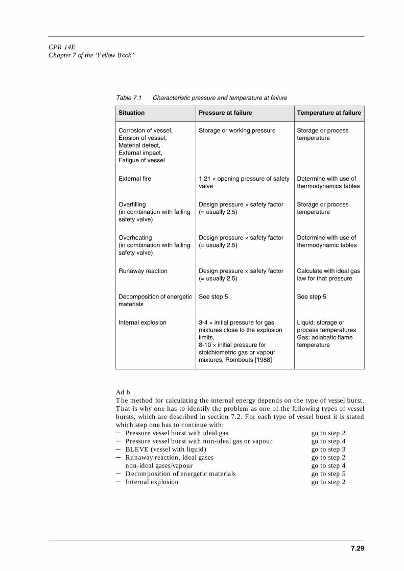
CPR 14EChapter 7 of the ‘Yellow Book’
7.29
Table 7.1 Characteristic pressure and temperature at failure
Ad bThe method for calculating the internal energy depends on the type of vessel burst.That is why one has to identify the problem as one of the following types of vesselbursts, which are described in section 7.2. For each type of vessel burst it is statedwhich step one has to continue with:– Pressure vessel burst with ideal gas go to step 2– Pressure vessel burst with non-ideal gas or vapour go to step 4– BLEVE (vessel with liquid) go to step 3– Runaway reaction, ideal gases go to step 2
non-ideal gases/vapour go to step 4– Decomposition of energetic materials go to step 5– Internal explosion go to step 2
Situation Pressure at failure Temperature at failure
Corrosion of vessel,Erosion of vessel,Material defect,External impact,Fatigue of vessel
Storage or working pressure Storage or process temperature
External fire 1.21 × opening pressure of safety valve
Determine with use of thermodynamics tables
Overfilling (in combination with failing safety valve)
Design pressure × safety factor (= usually 2.5)
Storage or process temperature
Overheating (in combination with failing safety valve)
Design pressure × safety factor (= usually 2.5)
Determine with use of thermodynamic tables
Runaway reaction Design pressure × safety factor (= usually 2.5)
Calculate with ideal gas law for that pressure
Decomposition of energetic materials
See step 5 See step 5
Internal explosion 3-4 × initial pressure for gas mixtures close to the explosion limits,8-10 × initial pressure for stoichiometric gas or vapour mixtures, Rombouts [1988]
Liquid: storage or process temperaturesGas: adiabatic flame temperature

7.30
Step 2 Calculation of the liberated energy of a pressure vessel burst or runaway reactionwith an ideal gas, or an internal explosion
The liberated energy Eav of a compressed gas as it expands to atmospheric pressureis calculated as follows:
(J) (7.1)
whereEav = liberated/expansion energy of compressed gas [J]p1 = absolute pressure of gas [Pa]pa = absolute pressure of ambient air [Pa]Vg = volume of gas-filled space of vessel [m3]γ1 = ratio of specific heats of gas in system [-]
Next: go to step 6.
Step 3 Check temperature of liquid
The temperature determines whether or not the liquid in a vessel will boil whendepressurised:Tl < Tb : the liquid will not boil, only the vapour in the vessel will
contribute to a blast wave (= pressure vessel burst withvapour)
Tb < Tl < Tsl : the liquid will boil, possibly BLEVETl > Tsl : the liquid will boil explosively, BLEVE
where:Tb = boiling temperature at atmospheric pressure [K]Tc = critical temperature (i.e. temperature above which
a gas cannot be liquefied by pressure alone) [K]Tsl = superheat limit temperature at atmospheric pressure,
approximately equal to 0.89 × Tc for many fluids [K]
If the liquid is a mixture of fluids, consider each fluid separately.Continue with step 4.
Step 4 Calculation of the liberated energy in case of a vessel burst or runaway reaction witha non-ideal gas or vapour or liquid (BLEVE)
Step 4a Determine if the fluid is given in Table 7.2 or Figure 7.3
The work performed by a fluid as it expands has been calculated for the followingseven common fluids:– ammonia– carbon dioxide– ethane– isobutane– nitrogen
Eavp1 pa–( ) Vg×
γ1 1–-------------------------------=

CPR 14EChapter 7 of the ‘Yellow Book’
7.31
– oxygen– propane
If the fluid of interest is listed, go to step 4d. If not, go to step 4b.
Step 4b Determine internal energy in initial state, u1
The work done by an expanding fluid (i.e., a liquid or a vapour) is defined as thedifference in internal energy u between the fluid’s initial and final states. Mostthermodynamic tables and graphs do not present u but only the enthalpy h, absolutepressure p, specific volume v, absolute temperature T and the specific entropy s.Therefore, u must be calculated with the following equation:
u = h - pv (J/kg) (7.2)
whereu = specific internal energy [J/kg]h = specific enthalpy (enthalpy per unit mass) [J/kg]p = absolute pressure [Pa]v = specific volume [m3/kg]
To use a thermodynamic graph, locate the fluid’s initial state on the graph. (For asaturated fluid, this point lies either on the saturated liquid or on the saturated vapourcurve, at a pressure p1.) Read the enthalpy h1, volume v1, and entropy s1 from thegraph. If thermodynamic tables are used, interpolate these values from the tables.Calculate the specific internal energy in the initial state u1 with equation (7.2), bothfor the vapour phase and the liquid phase.The thermodynamic properties of mixtures of fluids are usually not known. A crudeestimate of a mixture’s internal energy can be made by summing up the internalenergy of each component.Continue with step 4c.
Step 4c Determine internal energy in expanded state, u2
The specific internal energy of the fluid in the expanded state u2 can be determinedas follows: If a thermodynamic graph is used, assume an isentropic expansion(entropy s is constant) to atmospheric pressure pa. Therefore, follow the constant-entropy line from the initial state to pa. Read h2 and v2 at this point, and calculate thespecific internal energy u2 by using of equation (7.2). This is illustrated in example 1in section 7.6.2.If thermodynamic tables are used, read the enthalpy hf, volume vf, and entropy sf ofthe saturated liquid at ambient pressure, pa, interpolating if necessary. In the sameway, read these values (hg, vg, sg) for the saturated vapour state at ambient pressure.Then, use the following equation to calculate the specific internal energy u2:
u2 = (1 - X)hf + Xhg - (1 - X)pavf - Xpavg (J/kg) (7.3)
whereX = vapour ratio (s1 - sf)/(sg - sf) [-]s = specific entropy [J/(kg⋅K)]
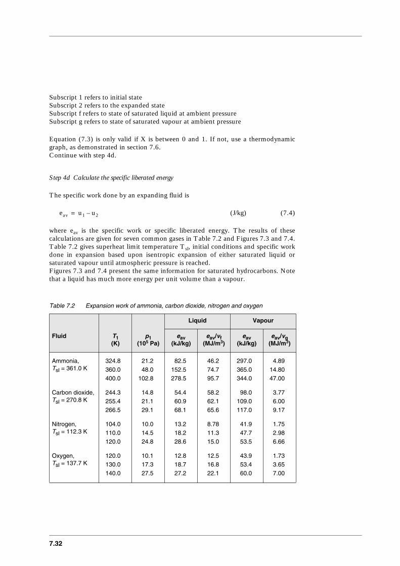
7.32
Subscript 1 refers to initial stateSubscript 2 refers to the expanded stateSubscript f refers to state of saturated liquid at ambient pressureSubscript g refers to state of saturated vapour at ambient pressure
Equation (7.3) is only valid if X is between 0 and 1. If not, use a thermodynamicgraph, as demonstrated in section 7.6.Continue with step 4d.
Step 4d Calculate the specific liberated energy
The specific work done by an expanding fluid is
(J/kg) (7.4)
where eav is the specific work or specific liberated energy. The results of thesecalculations are given for seven common gases in Table 7.2 and Figures 7.3 and 7.4.Table 7.2 gives superheat limit temperature Tsl, initial conditions and specific workdone in expansion based upon isentropic expansion of either saturated liquid orsaturated vapour until atmospheric pressure is reached.Figures 7.3 and 7.4 present the same information for saturated hydrocarbons. Notethat a liquid has much more energy per unit volume than a vapour.
Table 7.2 Expansion work of ammonia, carbon dioxide, nitrogen and oxygen
Liquid Vapour
Fluid T1 (K)
p1 (105 Pa)
eav (kJ/kg)
eav/vf (MJ/m3)
eav (kJ/kg)
eav/vg (MJ/m3)
Ammonia, Tsl = 361.0 K
324.8 21.2 82.5 46.2 297.0 4.89360.0 48.0 152.5 74.7 365.0 14.80400.0 102.8 278.5 95.7 344.0 47.00
Carbon dioxide, Tsl = 270.8 K
244.3 14.8 54.4 58.2 98.0 3.77255.4 21.1 60.9 62.1 109.0 6.00266.5 29.1 68.1 65.6 117.0 9.17
Nitrogen, Tsl = 112.3 K
104.0 10.0 13.2 8.78 41.9 1.75110.0 14.5 18.2 11.3 47.7 2.98120.0 24.8 28.6 15.0 53.5 6.66
Oxygen, Tsl = 137.7 K
120.0 10.1 12.8 12.5 43.9 1.73130.0 17.3 18.7 16.8 53.4 3.65140.0 27.5 27.2 22.1 60.0 7.00
eav u1 u2–=
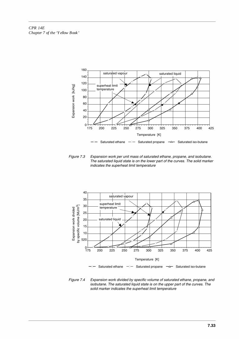
CPR 14EChapter 7 of the ‘Yellow Book’
7.33
Figure 7.3 Expansion work per unit mass of saturated ethane, propane, and isobutane. The saturated liquid state is on the lower part of the curves. The solid marker indicates the superheat limit temperature
Figure 7.4 Expansion work divided by specific volume of saturated ethane, propane, and isobutane. The saturated liquid state is on the upper part of the curves. The solid marker indicates the superheat limit temperature
20
40
60
80
100
120
140
160
175 200 225 250 275 300 325 350 375 400 425
Temperature [K]
Exp
ansi
on w
ork
[kJ/
kg]
Saturated ethane Saturated propane Saturated iso-butane
0
saturated vapour
superheat limit temperature
saturated liquid
175 200 225 250 275 300 325 350 375 400 425
Temperature [K]
Saturated ethane Saturated propane Saturated iso-butane
520
10
15
20
25
30
35
40
0
saturated vapour
saturated liquid
superheat limit temperature
Exp
ansi
on w
ork
divi
ded
by s
peci
fic v
olum
e [M
J/m
3 ]
7.34
Calculate the specific work done by the fluid for the vapour phase and the liquidphase, and in case of a mixture of fluids, for all components.Continue with step 4e.
Step 4e Calculate total liberated energy
To calculate the available energy, multiply the specific expansion work by the mass ofthe phase or component of the fluid released or else, if energy per unit volume is used,multiply by the volume of the phase or component of the fluid released.
Eav = eav × Mfl (J) (7.5a)
Eav = (eav/v) × Vfl (J) (7.5b)
whereMfl = mass of released phase or component of the fluid [kg]Vfl = volume of released phase or component of the fluid [m3]
Repeat steps 4b to 4e for each phase and component present in the vessel, and addthe energies to find the total liberated energy Eav. When this total energy has beenfound, go to step 6.
Step 5 Determine the available energy for a decomposition of an energetic material
For a decomposition of an energetic material it is not possible to give an unequivocaladvice on the failure pressure. A different approach to calculate the liberated energyis therefore necessary.The upper limit for the liberated energy is given by the total amount of chemicalenergy of the decomposition. This is shown by an example.
The heat of reaction can be found from the difference between the heat of formationof the reactants and that of the reaction products. Yoshida [1987] gives an examplefor the detonative decomposition of nitromethane. The heats of formation of thereactants and reaction products, in kJ/mol, are given below the stoichiometicequation.
CH3NO2 (l) → (3/2) H2O (l) + (1/4) CO2 (g) + (1/2) N2 (g) + (3/4) C (s)
-∆Hf 113.4 287.3 395.2 0 0
The heat of reaction ∆Hf is: (3/2) × 287.3 + (1/4) × 395.2 - 113.4 = 416.4 kJ/mol, or6.8 MJ/kg nitromethane. For more information see Yoshida [1987].The total chemical energy can now be found by multiplying the heat of reaction withthe total mass of product:
Eav = Mc ∆Hf (J) (7.6)
where∆Hf = the heat of reaction per kg product [J/kg]Mc = the total mass of contents of the vessel [kg]

CPR 14EChapter 7 of the ‘Yellow Book’
7.35
This method will considerably overestimate the explosion effects in most cases,because often only part of the vessel’s contents decomposes or does not decomposequickly enough to contribute to the blast.Continue with step 6.
Step 6 Determine the effective blast wave energy, Eex
The effective blast wave energy is given by
Eex = Asb × Eav (J) (7.7)
In this equation it is assumed that all available energy will be converted into blastwave energy. With the factor Asb, the presence of a reflecting ground surface can betaken into account. Asb = 1, when the vessel is high in the air, Asb = 2 when the vesselis less than 15 degrees above the horizon, as seen from the target. Note that this method only predicts the peak overpressure of the incident shock wave.The target may receive additional loadings from reflected shock waves. This isespecially the case when the vessel is high in the air. To find the total load in thesecases, use the methods described in TM 5-1300 [1990] or consult an expert.Continue with step 7.
Step 7 Calculate R of the target
The non-dimensional distance of the so-called ‘target’, R, is defined as
(-) (7.8)
where rt is the distance in metres at which blast parameters are to be determined.Continue with step 8.
Step 8: Check the value of R
For R ≥ 2 the basic method gives good results. For R < 2 however, the basic methodgives too high a value. A refined method is available for pressure vessel bursts orrunaway reactions with ideal gas.Therefore, continue according to the following list:
R ≥ 2, continue with step 9.R < 2, ideal gas go to step 10.R < 2, other vessel bursts continue with step 9 and realise that the results
will be conservative.
Step 9 Determine Ps for all types of vessel bursts except for a pressure vessel burst with anideal gas at close range (R < 2)
Ps is the non-dimensional side-on overpressure of the blast wave. This non-dimensional overpressure can be read from Figure 7.5 or 7.6 for the appropriate R.Use the curve labelled ‘high explosive’ if Figure 7.5 is used.Next: go to step 11.
R rt
pa
Eex-------
1 3/=

7.36
Figure 7.5 Non-dimensional overpressure versus non-dimensional distance for overpressure calculations, Baker et al. [1977].R = rt (pa / Eex)1/3 and Ps = ps / pa - 1
CPR 14EChapter 7 of the ‘Yellow Book’
7.37
Figure 7.6 Ps versus R for pentolite, Baker et al. [1977].R = rt (pa / Eex)1/3, Ps = ps / pa -1

7.38
Step 10 Determine Ps for a pressure vessel burst with an ideal gas and R < 2 (Refined method for the near field)
Because the similarity of the blast waves of vessel bursts and high explosives does nothold for the near field, a refined method is necessary to predict the blast pressures.
Step 10a Collect additional data
In addition to the data collected in step 1 of the basic method, the following data isneeded:– the ratio of the speed of sound in the compressed gas to its speed in ambient air,
a1/aa;– the ratio of specific heats of ambient air, γa = 1.40, the molar mass is
0.0290 kg/mol.
For an ideal gas (a1/aa)2 is
(-) (7.9)
whereTa = absolute temperature of ambient air [K]Tg = absolute temperature of compressed gas [K]µ1 = molar mass of compressed gas [kg/mol]µa = molar mass of ambient air [kg/mol]γa and γ1 are specific heat ratios [-]
Continue with step 10b.
Step 10b Calculate the initial distance
This refined method assumes the blast wave to be completely symmetrical. Such ashape would result from the explosion of a hemispherical vessel placed directly on theground. Therefore, a hemispherical vessel is used instead of the actual vessel forcalculation purposes.Calculate the hemispherical vessel’s radius r0 from the volume of the gas-filled part ofthe actual vessel Vg:
(m) (7.10)
This is the starting distance on the overpressure versus distance curve. It must betransformed into the non-dimensional starting distance, R0, with:
(-) (7.11)
Continue with step 10c.
a1
aa----
2 γ1Tgµa
γ aTaµ1-----------------=
r0
3Vg
2π---------
1 3/
0.782 Vg1 3/×= =
R0 r0
pa
Eex-------
1 3/=
CPR 14EChapter 7 of the ‘Yellow Book’
7.39
Step 10c Calculate the initial peak overpressure Pso
The peak shock pressure directly after the burst, pso, is much lower than the initial gaspressure in the vessel p1. The non-dimensional peak shock overpressure directly afterthe burst, Pso, is defined as (pso/pa) - 1. It is given by the following expression:
(-) (7.12)
wherep1 = initial absolute pressure of compressed gas [Pa]pa = ambient pressure [Pa]Pso = non-dimensional peak shock overpressure directly
after burst:Pso = (pso / pa) − 1 [-]
pso = peak shock pressure directly after burst [Pa]γa = ratio of specific heats of ambient air [-]γ1 = ratio of specific heats of compressed gas [-]aa = speed of sound in ambient air [m/s]a1 = speed of sound in compressed gas [m/s]
This is an implicit equation which can only be solved by iteration. One might use aspreadsheet to solve Pso. An alternative is to read Pso from Figure 7.7 or 7.8.
Figure 7.7 Gas temperature versus pressure for constant Pso for γ1 = 1.4,Baker et al. [1977]
p1
pa----- Pso 1+( ) 1
γ1 1–( ) aa/a1( )Pso
2γ a 2γ a γ( a 1 )+ + Pso( )[ ]1 2/----------------------------------------------------------------–
2– γ1
γ1 1–-------------
=
7.40
Figure 7.8 Gas temperature versus pressure for constant Pso for γ1= 1.66, Baker et al. [1977]
Continue with step 10d.
Step 10d Locate the starting point of Figure 7.5
In steps 10b and 10c, the vessel’s non-dimensional radius and the blast wave’s non-dimensional peak pressure at that radius were calculated. As a blast wave travelsoutward, its pressure decreases rapidly. The relationship between the peak pressurePs and the distance R depends upon the initial conditions. Accordingly, Figure 7.5contains several curves. Locate the correct curve by plotting (R, Pso) in the figure.Continue with step 10e.
Step 10e Determine Ps
To determine the non-dimensional side-on overpressure Ps, read Ps from Figure 7.5for the appropriate R (calculated in step 7). Use the curve which goes through thestarting point, or else draw a curve through the starting point parallel to the nearestcurve.Continue with step 11.
Step 11 Determine I
To determine the non-dimensional side-on impulse I, read I from Figure 7.9 or 7.10for the appropriate R. Use the curve labelled as ‘vessel burst’. For R in the range of0.1 to 1.0, the I versus R curve of Figure 7.10 is more convenient.Continue with step 12.

CPR 14EChapter 7 of the ‘Yellow Book’
7.41
Figure 7.9 I versus R for pentolite and gas vessel bursts, Baker et al. [1977],R = rt (pa / Eex)1/3, I = (isaa) / ( )pa
2 3/ E ex1 3/
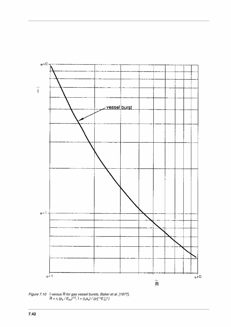
7.42
Figure 7.10 I versus R for gas vessel bursts, Baker et al. [1977],R = rt (pa / Eex)1/3, I = (isaa) / ( )pa
2 3/ E ex1 3/

CPR 14EChapter 7 of the ‘Yellow Book’
7.43
Step 12 Adjust Ps and I for geometry effects
The above procedure gives blast parameters applicable to a completely symmetricalblast wave, such as would result from the expansion of a hemispherical vessel abovethe ground or a spherical vessel in free air. In practice, vessels are either spherical orcylindrical, and placed at some height above the ground. This influences blastparameters. To adjust for these geometry effects, Ps and I must be multiplied by someadjustment factors. Table 7.3 and 7.4 give multiplication factors for adjusting thescaled values for cylindrical vessels of various R and for vessels elevated slightly abovethe ground, respectively.It must be mentioned that for cylindrical vessels the blast field is asymmetrical whenplaced horizontally. The blast wave is weakest along the axis. The correction methodwill only provide the maximum values for a horizontal tank.Continue with step 13.
Table 7.3 Adjustment factors for Ps and I for cylindrical vessels for various R
Table 7.4 Adjustment factors for Psand I for vessels slightly elevated above the ground
Step 13 Calculate ps, is
Use the following equations to calculate the side-on peak overpressure ps - pa and theside-on impulse is from the non-dimensional side-on peak overpressure Ps and thenon-dimensional side-on impulse I:
(Pa) (7.13)
(Pa⋅s) (7.14)
Multiplier for
R Ps I
< 0.3≥ 0.3 and ≤ 1.6>1.6 and ≤ 3.5>3.5
41.61.61.4
21.111
Multiplier for
R Ps I
< 1≥ 1
21.1
1.61
ps pa– Ps pa×=
isI pa
2 3/ Eex1 3/××
aa---------------------------------=

7.44
where aa is the speed of sound in ambient air in metres per second. For sea-levelaverage conditions, pa is approximately 101.3 kPa and aa is 340 m/s.Continue with step 14.
Step 14 Check ps
This method has only a limited accuracy, especially in the near field. Under somecircumstances, the calculated ps might be higher than the initial pressure in the vesselp1, which is physically impossible. If this should happen, take p1 as the peak pressureinstead of the calculated ps.
Note that the methods presented above give upper estimates of blast parameters. Inpractice, overpressures in one case might very well be much lower than predicted bythe method, and in another case they might be close to the predicted value.The method is therefore not suitable for analysis of accidents. It is just a tool topredict safe upper values for plant layout etc.
7.5.3 Methods for fragmentation effects
The risk from fragments at a particular location is related to the number offragments that may fall on or fly through that location and their potential to dodamage, i.e. their mass and velocity.
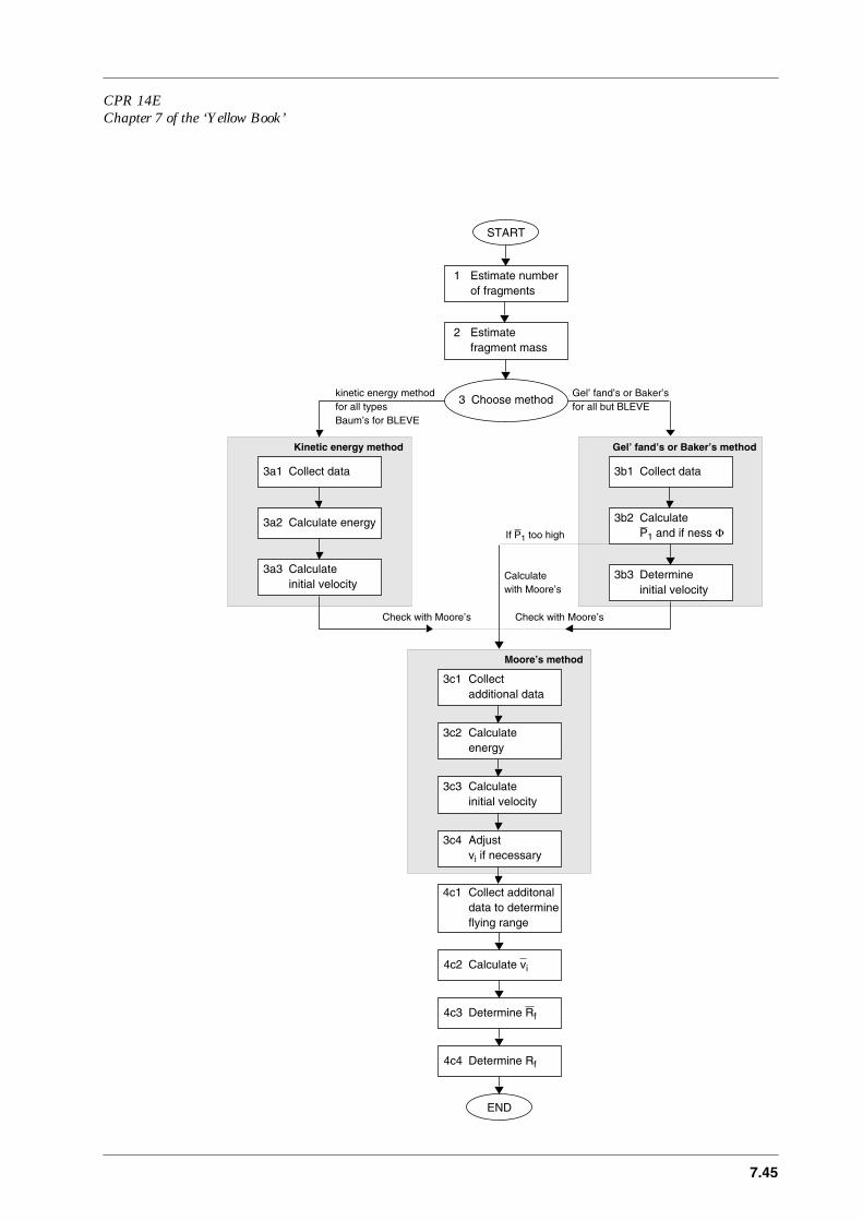
CPR 14EChapter 7 of the ‘Yellow Book’
7.45
Choose method3
END
START
Gel’ fand’s or Baker’s
Estimate number1of fragments
Estimatefragment mass
for all but BLEVEkinetic energy methodfor all types
Collect data3a1
Calculate energy3a2
Calculate3a3initial velocity
Baum’s for BLEVE
Kinetic energy method
Collect data3b1
Determine3b3initial velocity
Gel’ fand’s or Baker’s method
Calculate3b2P1 and if ness Φ
Check with Moore’s Check with Moore’s
If P1 too high
Calculatewith Moore’s
Calculate3c3initial velocity
Moore’s method
Calculate3c2energy
Collect3c1additional data
Collect additonal4c1data to determine
Adjust3c4vi if necessary
flying range
Calculate vi4c2
Determine Rf4c3
Determine Rf4c4
2

7.46
Step 1 Estimate number of fragments
There are no methods to predict the number of fragments. An estimate of the numberof fragments can only be made by using a pragmatic approach which is based onanalyses of accidental explosions.A pragmatic approach to estimate the number of fragments to be expected issummarised in Table 7.5. It means that in case of a local weakening of the vessel it ismost probable that it will break into two pieces, whereas in case of overpressure thevessel will break into more pieces, usually along the welds. A cylinder usually has onlya few welds whereas a sphere has much more welds.
Table 7.5 Pragmatic approach to estimate number of fragments
Continue with step 2.
Step 2 Estimate fragment mass, Mf
As is the case for the number of fragments, there is no method available to estimatethe mass of the fragment. Only a pragmatic approach can be used.This pragmatic approach is related to the pragmatic approach for the determinationof the number of fragments. Knowing this number nf, it is easy to calculate theaverage mass of the fragments, being equal to Mv/nf.This estimate of the average fragment mass can be considered as reasonable in caseof rupture into many fragments or in case of rupture into a few equal fragments. Thisis the case for spheres.Cylinders, however, usually do not break into equal parts. They usually break at theend caps. The vessel often projects its end caps along the axis of the vessel and theunfolded shell perpendicular to the vessel’s axis.A survey of possible fragments is given in Table 7.6.
Situation Number of fragments
Local weakening 2 pieces
OverpressureCylinderSphere
2 or 3 pieces10 to 20 pieces

CPR 14EChapter 7 of the ‘Yellow Book’
7.47
Table 7.6 Fragment mass and shape, pragmatic approach
Continue with step 3.
Step 3 Calculate fragment velocity
Calculate the fragment velocity according to one of the methods in Table 7.7.
Table 7.7 Selection of methods for fragmentation effects, depending on the type of burst
Check the results of the other methods (step 3a and 3b) with the empirical relation ofMoore (3c).
Step 3a Kinetic energy method to roughly predict the initial fragment velocity and Baum’sempirical formula for BLEVEs
The theoretical upper limit and a rough estimate of the initial fragment velocity canbe calculated as follows.
Type of vessel Fragment mass Mf Fragment shape
Sphere, 2 fragments Mv/2 hemisphere
Sphere, many fragments Mv/nf plates
Cylinder, 2 equal pieces Mv/2 half of tank
Cylinder, 2 unequal pieces 1 piece: Mcapother piece: Mv-Mcap
cap/hemispheretank with one cap missing
Cylinder, 3 unequal pieces 2 pieces: Mcapother: (Mv-2Mcap)
cap/hemisphereplate
Cylinder, many pieces 2 pieces: Mcaprest: (Mv-2Mcap)/(nf-2)
cap/hemispherestrip
Type of burst Method Go to step
Rough estimate for all types of vessel bursts, except decomposition of energetic materials
Kinetic energy method 3a
Pressure vessel burst Baker’s and/or Gel’fand’s method
3b
Runaway reaction, internal explosion Gel’fand’s method 3b
BLEVE Baum’s empirical formula 3a
For high scaled pressures and decomposition of energetic materials
Moore’s empirical relation 3c
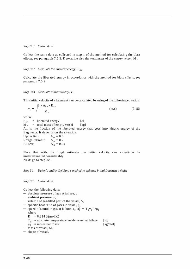
7.48
Step 3a1 Collect data
Collect the same data as collected in step 1 of the method for calculating the blasteffects, see paragraph 7.5.2. Determine also the total mass of the empty vessel, Mv.
Step 3a2 Calculate the liberated energy, Eav
Calculate the liberated energy in accordance with the method for blast effects, seeparagraph 7.5.2.
Step 3a3 Calculate initial velocity, vi
This initial velocity of a fragment can be calculated by using of the following equation:
(m/s) (7.15)
whereEav = liberated energy [J]Mv = total mass of empty vessel [kg]Ake is the fraction of the liberated energy that goes into kinetic energy of thefragments. It depends on the situation.Upper limit Ake = 0.6Rough estimate Ake = 0.2BLEVE Ake = 0.04
Note that with the rough estimate the initial velocity can sometimes beunderestimated considerably.Next: go to step 3c.
Step 3b Baker’s and/or Gel’fand’s method to estimate initial fragment velocity
Step 3b1 Collect data
Collect the following data:– absolute pressure of gas at failure, p1– ambient pressure, pa– volume of gas-filled part of the vessel, Vg– specific heat ratio of gases in vessel, γ1– speed of sound in gas at failure, a1,
whereR = 8.314 J/(mol⋅K)Tg = absolute temperature inside vessel at failure [K]µ1 = molecular mass [kg/mol]
– mass of vessel, Mv– shape of vessel.
vi
2 Ake Eav××
Mv
------------------------------=
a12 Tgγ1R/µ1=

CPR 14EChapter 7 of the ‘Yellow Book’
7.49
In case of a runaway reaction or internal explosion collect also the following data:– maximum laminar burning velocity of reaction, uf. For a few gases uf is given in
Table 5.1 in chapter ‘Vapour Cloud Explosions’.– heat of reaction per kg of the product, ∆Hf, which follows from the stoichiometric
equation for the reaction, see section 7.5.2, step 5.
Step 3b2 Calculate the dimensionless scaled overpressure P1
Calculate the scaled overpressure according to:
(-) (7.16)
In case of a runaway reaction or internal explosion also calculate the dimensionlessparameter Φ, which characterises the rate of energy release. Φ is given by:
(-) (7.17)
Step 3b3 Read vi from Figure 7.11
Choose the proper chart from Figures 7.11. Choose the proper line in this chart andread vi/a1 for P1, as determined in the previous step. If one can choose betweenBaker’s solution and the solution of Gel’fand, it is best to choose the mostconservative solution. Since a1 has been determined in step 3b1, the initial velocity viis now known.In case of a runaway reaction the proper line in the chart is determined by thedimensionless parameter Φ as calculated in step 3b2 and by the specific heat ratio γ1.The lines in the chart for a certain γ1 are in the same order as in the legend.In case of a cylinder with a different length-diameter ratio than in the figures, oneshould determine vi/a1 by interpolating between the values for the two closest vessels.Continue with step 3c.
P1 p1 pa–( ) Vg× / Mva12( )=
Φ∆Hf uf×
a13--------------------=
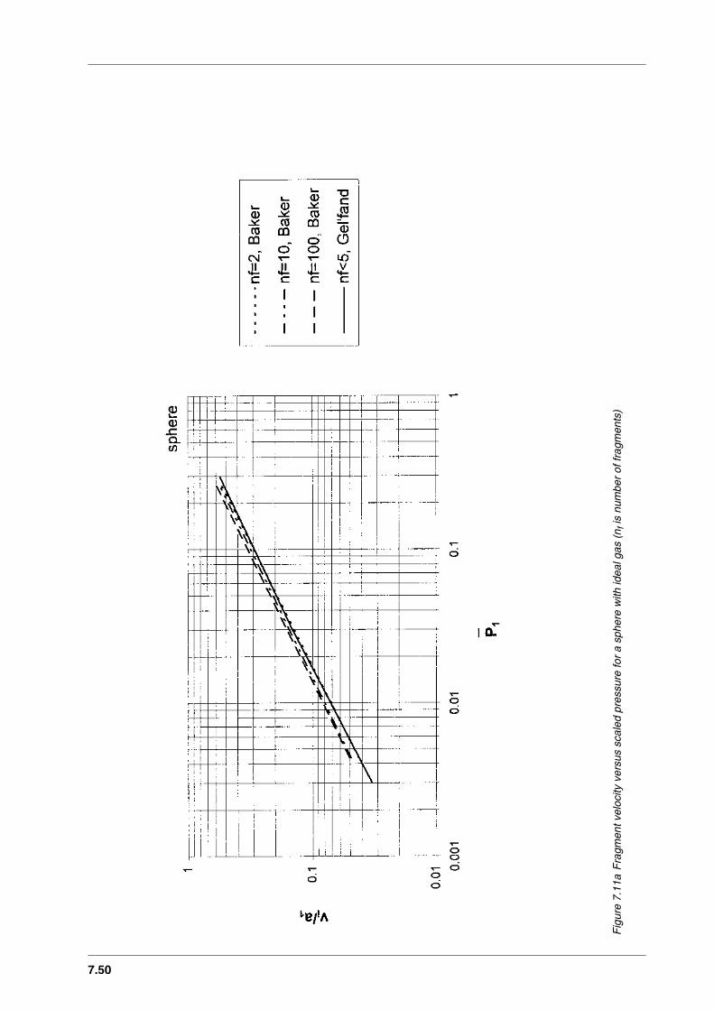
7.50
Fig
ure
7.11
aF
ragm
ent v
eloc
ity v
ersu
s sc
aled
pre
ssur
e fo
r a
sphe
re w
ith id
eal g
as (
n f is
num
ber
of fr
agm
ents
)
CPR 14EChapter 7 of the ‘Yellow Book’
7.51
Fig
ure
7.11
bF
ragm
ent v
eloc
ity v
ersu
s sc
aled
pre
ssur
e fo
r a
cylin
der
with
a le
ngth
-dia
met
er r
atio
of 5
, fill
ed w
ith a
n id
eal g
as (
n f is
num
ber
of fr
agm
ents
)
7.52
Fig
ure
7.11
cF
ragm
ent v
eloc
ity v
ersu
s sc
aled
pre
ssur
e fo
r a
cylin
der
with
a le
ngth
-dia
met
er r
atio
of 1
0, fi
lled
with
an
idea
l gas
(n f
is n
umbe
r of
frag
men
ts)
CPR 14EChapter 7 of the ‘Yellow Book’
7.53
Fig
ure
7.11
dF
ragm
ent v
eloc
ity v
ersu
s sc
aled
pre
ssur
e fo
r a
sphe
re, r
uptu
red
beca
use
of a
run
away
rea
ctio
n (li
nes
are
in th
e sa
me
orde
r as
in th
e le
gend
).
7.54
Fig
ure
7.11
eF
ragm
ent v
eloc
ity v
ersu
s sc
aled
pre
ssur
e fo
r a
cylin
der
with
a le
ngth
-dia
met
er r
atio
of 5
, rup
ture
d be
caus
e of
a r
unaw
ay r
eact
ion
(line
s ar
e in
the
sam
e or
der
as in
the
lege
nd).

CPR 14EChapter 7 of the ‘Yellow Book’
7.55
Fig
ure
7.11
fF
ragm
ent v
eloc
ity v
ersu
s sc
aled
pre
ssur
e fo
r a
cylin
der
with
a le
ngth
-dia
met
er r
atio
of 1
0, r
uptu
red
beca
use
of a
run
away
rea
ctio
n (li
nes
are
in th
e sa
me
orde
r as
in th
e le
gend
).
7.56
Step 3c Moore’s empirical formula for the initial fragment velocity in case of a high scaledpressure P1, decomposition of energetic materials, or to check the calculated vi.
Step 3c1 Collect data
Collect the same data as collected in step 1 of the method for calculating the blasteffects, see paragraph 7.5.2. Determine also the total mass of the empty vessel Mv andthe mass of the gas inside the vessel Mc.
Step 3c2 Calculate the liberated energy, Eav
Calculate the liberated energy in accordance with the method for blast effects, seeparagraph 7.5.2.
Step 3c3 Calculate initial velocity, vi
This initial velocity can be calculated by using of the following equation:
(m/s) (7.18)
where for spherical vessels (-) (7.19)
and for cylindrical vessels (-) (7.20)
Step 3c4 Check vi, calculated according to other method
If the initial velocity calculated before is higher than according to Moore’s empiricalrelation, then this velocity is too high. Use the value found with Moore’s equation.Continue with step 4.
Step 4 Calculate range of flying fragments
After a fragment is accelerated to a certain initial velocity, the forces acting upon itduring flight are those of gravity and fluid dynamics (lift and drag). These forcesdetermine the distance a fragment can fly.
Figure 7.12 plots scaled maximum range Rf and scaled initial velocity vi as a functionof the lift-to-drag ratio CLAL/CDAD. This figure is based on the assumption thatfragment orientation remains constant with respect to the trajectory (constant angleof attack). The scaled parameters are defined by
vi 1.092EavAM
Mv----------------
0.5=
AM1
1 3Mc/5Mv+--------------------------------=
AM1
1 Mc/2Mv+-----------------------------=

CPR 14EChapter 7 of the ‘Yellow Book’
7.57
(-) (7.21)
(-) (7.22)
where
Rf = scaled maximal range [-]Rf = maximal range [m]vi = scaled initial velocity [-]vi = initial velocity [m/s]ρa = density of ambient atmosphere [kg/m3]CD = drag coefficient [-]CL = lift coefficient [-]AD = exposed area in plane perpendicular to trajectory [m2]AL = exposed area in plane parallel to trajectory [m2]g = gravitational acceleration [m/s2]Mf = mass of fragment [kg]
Figure 7.12 Scaled curves for fragment range predictions. ----: solution for no wind resistance,
Using Figure 7.12 the maximum fragment range can be predicted as follows.
Step 4a Determine the following parameters– ρa, density of ambient atmosphere (kg/m3)– the (average) value for CDAD (m2), by using Table 7.8. The average value is
needed in case of tumbling, which often occurs.– the value for the lift-to-drag ratio CLAL/CDAD, with use of Table 7.8. For blunt
and tumbling objects the lift equals zero.
RfρaCDADRf
Mf--------------------------=
viρaCDADvi
2
Mfg--------------------------=
Rf v i2/g=
7.58
Table 7.8 Drag and lift of fragments
Step 4b Calculate the scaled initial velocity
The scaled initial velocity is given by equation (7.22).
(-) (7.22)
Step 4c Read scaled maximal range from Figure 7.12
Step 4d Calculate Rf
By using of equation (7.21) the maximal range Rf can be calculated.
(-) (7.21)
Shape CDAD CLAL/CDAD
Plate (tumbling) 0.585 × Aplate 0Plate (no tumbling, face on) 1.17 × Aplate 0Plate (no tumbling, edge on) 0.1 × Aplate 0 to 101)
1) The value depends on the plate’s angle. Use the value which gives the maximum fragment range, or calculate a number of possible ranges.
Hemisphere (tumbling) 0.615 × π/4 × dv2 0
Hemisphere (no tumbling) 0.47 × π/4 × dv2 0
Half a tank (rocketing) 0.47 × π/4 × dv2 0
Cylinder (edge on) 1.20 × dv × Lv 0Strips (tumbling) 0.99 × Astrip 0
viρaCDADvi
2
Mfg--------------------------=
RfρaCDADRf
Mf--------------------------=
CPR 14EChapter 7 of the ‘Yellow Book’
7.59
7.6 Application of selected methods: calculation examples
7.6.1 Introduction to section 7.6
Bursting vessels can generate blast and propel fragments to several hundredmetres distance. In this section calculation methods to predict the hazards of vesselbursts are demonstrated. The calculation methods have been described insection 7.5.Section 7.6.2 and 7.6.3 respectively provide examples of blast effects and offragmentation effects. In all these examples, one tank is considered with itsenvironment. Different types of vessel bursts are studied by assuming differentcontents for the tank.In the examples, data are just listed and equations are used without repeating them.The numbers of the equations are given, so that the reader can easily retrace them insection 7.5. Decision points are explained in accordance with the flow charts.Like the description of the test method, the examples are also presented stepwise. Thenumbers of each step in the examples correspond to those in the description of themethods and in the chart flows.
7.6.2 Example 1: blast effects
Consider a cylindrical vessel, used for the storage of propane, which hasbeen repaired. After the repair, the vessel is pressure tested with nitrogen gas at apressure 25% above the design pressure. If the vessel bursts during the test, a largestorage tank, located 15 m from the vessel, and a control building, located 100 mfrom the vessel, might be endangered. What would be the side-on overpressure andimpulse at these points?After a successful pressure test, the vessel is re-entered into service. The safety valveis set at 1.5 MPa (15 bar) overpressure. What might happen if the vessel was exposedto a fire? Consider the vessel being filled for 80% with propane.
Solution for gas-filled vessel
Step 1 Collect data
a. Nitrogen at ambient temperature can be regarded as an ideal gas.b. Since the vessel contains an ideal gas, we are dealing with a pressure vessel burst.c. The design overpressure of the vessel is 1.92 MPa, the test pressure is 25% higher.
Therefore, the absolute internal pressure p1 is:
p1 = 1.25 × 1.92 × 106 + 0.1 × 106 = 2.5 MPa (25 bar)
d. The ambient pressure pa is 101325 Pa.e. The volume of the vessel is 25 m3.f. The ratio of specific heats of nitrogen, γ1, is 1.40.g. The distance from the centre of the vessel to the ‘target’, rt, is 100 m for the
control building and 15 m for the large storage tank.h. The shape of the vessel is cylindrical. It is placed horizontally, on the ground.
7.60
Step 2 Energy calculation
The energy of the compressed gas is calculated using equation (7.1).Substitution gives:
Step 6 Effective blast energy
Assuming that all energy is available for blast energy and using the fact that the vesselis placed on the ground, the calculated liberated energy must be multiplied by a factor2 in order to obtain the effective blast energy. So, Eex = 300 MJ.
Step 7 Calculate the non-dimensional distance R of the acceptor.
The non-dimensional range R is calculated using equation (7.8).Substitution gives for the control building:
And for the large storage tank: R = 1.05
Step 8 Check R
The non-dimensional range R is checked to see whether the basic method can befollowed or the refined method must be used. The control building lies at a non-dimensional range of 6.9, so the basic method can be followed. The range of the largestorage tank is less than 2, so the refined method must be used to obtain an accurateresult.
First, the blast parameters at the control building will be determined.
Step 9 Determine Ps
The non-dimensional side-on peak overpressure Ps at the control building is readfrom Figure 7.6. For R = 6.9, Ps = 0.028.
Step 11 Determine I
The non-dimensional side-on impulse I at the control building is read fromFigure 7.10. For R = 6.9, I = 0.0075.
Eav2.5 106 0.1 106×–×( ) 25×
1.4 1–----------------------------------------------------------------- 150 MJ= =
R 100 0.1 106×
300 106×-----------------------
1/3× 6.97= =
CPR 14EChapter 7 of the ‘Yellow Book’
7.61
Step 12 Adjust Ps and I for geometry effects
To account for the fact that the blast wave from the vessel will not be perfectlysymmetrical, Ps and I are adjusted, depending on R. To account for a cylindricalvessel, Ps is multiplied by 1.4. Thus, Ps becomes:
Ps = 1.4 × 0.028 = 0.0391
No adjustment of I is necessary at this range.
Step 13 Calculate ps and is
To calculate the side-on peak overpressure ps - pa and the side-on impulse is from thenon-dimensional side-on peak overpressure Ps and the non-dimensional side-onimpulse I, equations (7.13) and (7.14) are used.The ambient speed of sound aa is approximately 340 m/s. Substitution gives:
ps - pa = 0.0391 × 101325 = 3.97 kPa
is = (0.0075 × (101325)2/3 × (300 × 106)1/3) / 340 = 32 Pa⋅s
Step 14 Check ps
Because the accuracy of this method is limited, ps needs to be checked against p1. Inthis case, ps is much smaller than p1, so no corrections have to be made.Thus, the calculated blast parameters at the control building are: a side-on peakoverpressure of 3.97 kPa and a side-on impulse of 32 Pa⋅s.
As shown above, the distance to the large storage tank is too small to use the basicmethod with good results. Therefore, the refined method is used to calculate the blastparameters at the large storage tank.
Step 10a Collect additional data
– The ratio of the speed of sound in the compressed nitrogen and the speed of soundin the ambient air, a1/aa, is approximately 1.
– The ratio of specific heats of the ambient air is 1.40.
Step 10b Calculate the starting distance
The starting distance is computed with equation (7.10). Substitution gives:
r0 = 0.782 × 251/3 = 2.29 m
7.62
r0 must be transformed into the non-dimensional starting distance R0 withequation 7.11. Substitution gives:
R0 = 2.29 × (0.1 × 106 / 300 × 106)1/3 = 0.16
Step 10c Calculate the initial peak overpressure Pso
The non-dimensional peak overpressure of the shock wave directly after the burst ofthe vessel, Pso, can be read from Figure 7.7. The result is: Pso = 3.05, eight times lessthan the initial pressure in the vessel.
Step 10d Locate the starting point on Figure 7.5
To select the proper curve in Figure 7.5, the starting point R0, Pso is drawn in thefigure.
Step 10e Determine Ps
To determine the non-dimensional side-on peak overpressure Ps at the large storagetank, Ps is read from Figure 7.5. The non-dimensional distance was computed beforeas R = 1.05. Following the curve from the starting point, a Ps of 0.36 is found. Theprocedure is continued with step 11.
Step 11 Determine I
The non-dimensional side-on impulse I at the tank is read from Figure 7.9. ForR = 1.05, I = 0.048.
Step 12 Adjust Ps and I for geometry effects
To account for the fact that the blast wave from the vessel will not be perfectlysymmetrical, Ps and I are adjusted, depending on R. To account for the vessel’splacement slightly above ground level, Ps is multiplied by 1.1. To account for thecylindrical shape of the vessel, Ps is multiplied by 1.6 and I is multiplied by 1.1. Thus,Ps and I become:
Ps = 1.6 × 0.36 = 0.576
I = 1.1 × 0.048 = 0.053
Step 13 Calculate ps and is
To calculate side-on peak overpressure ps - pa and side-on impulse is from the non-dimensional side-on peak overpressure Ps and the non-dimensional side-on impulseI, equation (7.13) and (7.14) are used.
CPR 14EChapter 7 of the ‘Yellow Book’
7.63
The ambient speed of sound aa is approximately 340 m/s. Substitution gives:
ps - pa = 0.576 × 101325 = 58 kPa
is = 0.053 × ( 101325)2/3 × (300 × 106)1/3) / 340 = 225 Pa⋅s
Step 14 Check ps
Because the accuracy of this method is limited, ps needs to be checked against p1. Inthis case, ps is much smaller than p1, so no corrections have to be made.Thus, the calculated blast parameters at the large storage vessel are: a side-on peakoverpressure of 63 kPa and a side-on impulse of 230 Pa.s.
Solution for liquid-filled vessel
Step 1 Collect data
a. The vessel contains pressure liquefied propane.b. The possible type of vessel burst is a BLEVE.c. The failure overpressure is assumed to be 1.21 times the opening pressure of the
safety valve. Thus, p1 is:
p1 = 1.21 × 1.5 + 0.1 = 1.9 MPa (19 bar)
d. The ambient pressure pa is assumed to be 101325 Pa.e. The volume of the vessel is 25 m3.f. The distance from the centre of the vessel to the receptor is 100 m for the control
building and 15 m for the large storage tank.g. The shape of the vessel is cylindrical. It is placed horizontally, on saddles.h. The ambient temperature is 293 K. The temperature of saturated propane at a
vapour pressure of 1.9 MPa is 327.7 K.
Step 3 Check temperature of liquid
The boiling temperature and superheat limit temperature are given in Perry andGreen [1984]: Tb = 231 K, Tsl = 326 K. The temperature of the propane is abovesuperheat limit temperature. So, a BLEVE may occur.
Step 4a Check if the fluid is in Table 7.2 or Figure 7.3
Although the specific expansion energy of propane is included in the list of fluids inFigure 7.3, steps 4b to 4d are followed for this demonstration. It will be demonstratedboth by using a thermodynamic graph and a thermodynamic table.

7.64
Step 4b and 4c using a thermodynamic table
Step 4b Determine u1
Thermodynamic data for propane can be found in e.g. Perry and Green [1984].These are presented in Table 7.9.
Table 7.9 Thermodynamic data for propane
The vessel is assumed to be filled with saturated liquid and vapour. The specificinternal energy of the saturated liquid can be computed by substituting theappropriate thermodynamic data of Table 7.9 in equation (7.2):
u1 = 674.31 × 10³ - 1.90 × 106 × 2.278 × 10-3
It follows that: u1 = 669.98 kJ/kg.The specific internal energy of the saturated vapour can be computed in the sameway:
u1 = 948.32 × 10³ - 1.90 × 106 × 0.0232 = 904.24 kJ/kg
Step 4c Determine u2
The specific internal energy of the fluid after expansion to the ambient pressure, u2,is calculated using equation (7.3).For the saturated liquid, the vapour ratio X is:
X = (4.7685 - 3.8721) / (5.7256 - 3.8721) = 0.484
and u2 is:
u2 = (1 - 0.484) × 421.27 × 103 + 0.484 × 849.19 × 103 -
(1 - 0.484) × 0.1 × 106 × 1.722 × 10-3 - 0.484 × 0.1 × 106 × 0.419
= 608.01 kJ/kg
For the saturated vapour, X = 0.935 and u2 = 782.19 kJ/kg
T1 (K)
p1
(MPa)hf
(kJ/kg)hg
(kJ/kg)vf
(m3/kg)vg
(m3/kg)sf
(kJ/kgK)sg
(kJ/kgK)
327.7230.9
1.900.10
674.31421.27
948.32849.19
2.278 × 10⁻³
1.722 × 10⁻³
0.02320.419
4.76853.8721
5.60515.7256

CPR 14EChapter 7 of the ‘Yellow Book’
7.65
Step 4b and 4c using a thermodynamic graph
Step 4b Determine u1
Figure 7.13 gives an schematic view of the enthalpy-pressure graph of propane.Clearly visible is the curve indicating the saturated state. The top of this curve is thecritical point. On the left of this point is the liquid state, and on the right the vapourstate. The graph also shows lines of constant temperature T, constant specific volumev, constant entropy s and constant vapour ratio X. The thermodynamic data can alsobe drawn in other types of graphs, e.g. an enthalpy-entropy graph.
Figure 7.13 Enthalpy-pressure graph of propane (schematic)
The vessel is assumed to be filled with saturated liquid and saturated vapour. Thespecific internal energy of the saturated liquid can be computed with equation (7.2).The initial state can be found on the graph by locating the point on the saturatedliquid curve which has a pressure of 1.9 MPa. The specific enthalpy of that state is674 kJ/kg. The specific volume of this state cannot be read from the graph. It can beassumed that it is negligible. This gives for the specific internal energy:
u1 = 674 × 103 - 1.90 × 106 × 0.0
It follows that: u1 = 674 kJ/kg.The specific internal energy of the saturated vapour can be computed the same way.In this case, the specific volume is not negligible.
u1 = 948 × 103 - 1.90 × 106 × 0.023 = 904.3 kJ/kg
7.66
Step 4c Determine u2
The state of the fluid after expansion can be found by following the constant entropycurve from the initial state to the state with atmospheric pressure. The final state is amixture of liquid and vapour if the initial state is saturated liquid or vapour. Thespecific enthalpy of the final state can be read directly from the graph:h2 = 6.28⋅103 J/kg. The specific volume must be computed from the vapour ratio Xin the final state and the specific volume v of the saturated liquid and vapour atatmospheric pressure.
v2 = (1 - X)vf + Xvg (m3/kg) (7.23)
In practice, the specific volume of the saturated liquid is negligible, so the specificvolume after expansion from the saturated liquid state becomes:
v2 = 0.48 × 0.42 = 0.20 m3/kg
This results in:
u2 = 628 × 103 - 0.1 × 106 × 0.20 = 608 kJ/kg
for the specific internal energy after expansion from the saturated liquid state.
Similarly, for expansion from the saturated vapour state the specific volume in thefinal state is 0.395 m3/kg and u2 = 782 kJ/kg
Step 4d Calculate the specific work
The specific work done by the fluid in expansion is calculated using equation 7.4.Substitution of the values for the saturated liquid gives:
eav = 669.98 × 10³ - 608.01 × 103 = 61.97 kJ/kg
and for the saturated vapour:
eav = 904.24 × 10³ - 782.19 × 103 = 122.05 kJ/kg
Note that these values could also have been read from Figure 7.3.
Step 4e Calculate the energy of the explosion
The energy of the explosion is calculated using equation (7.5). In this equation themass of the released liquid is given by dividing the volume of the released liquid by itsspecific volume.When the vessel is full, 80% of the volume is occupied by liquid. The mass of theliquid is approximately:
Mfl = 0.80 × 25 / 2.278 × 10-3 = 8780 kg
CPR 14EChapter 7 of the ‘Yellow Book’
7.67
In fact, the specific volume of propane at ambient temperature should have beenused, but that makes little difference in the result.
The mass of the vapour is:
Mfl = 0.20 × 25 / 0.0232 = 215.5 kg
For the explosion energy for the saturated liquid, this results in:
Eav = 61.97 × 103 × 8780 = 544.1 MJ
and for the saturated vapour:
Eav = 122.05 × 103 × 215.5 = 26.3 MJ
Assuming that the blast of the expansion of the vapour is synchronous with the blastfrom the flashing of the liquid, the total energy of the surface explosion is:
Eav = 544.1 × 10⁶ + 26.3 × 106 = 570.4 MJ
Step 6 Determine the effective blast wave energy
The available energy must be multiplied by 2 because it is a surface explosion. So,
Eex = 2 × 570.4 = 1140.8 MJ
Step 7 Calculate R of receptor
The non-dimensional range of the ‘target’ is calculated using equation (7.8). Thisresults for the large storage vessel in:
R = 15 × (101325 / 1140.8 × 106)1/3 = 0.67
and for the control building:
R = 100 × ( 101325 / 1140.8 × 106)1/3 = 4.5
Computations are continued with step 9.
Step 9 Determine Ps
The non-dimensional side-on peak overpressure Ps at the large storage tank is readfrom Figure 7.5. The non-dimensional distance R = 0.67. Reading from the curvelabelled ‘high explosive’, a Ps of 1.12 is found. The procedure is continued with step 11.

7.68
Step 11 Determine I
The non-dimensional side-on impulse I at the tank is read from Figure 7.10. ForR = 0.67, I = 0.068.
Step 12 Adjust Ps and I for geometry effects
To account for the fact that the blast wave from the vessel will not be perfectlysymmetrical, Ps and I are adjusted, depending on R. The multiplication factors toaccount for the cylindrical shape are taken from Tables 7.3 and 7.4. Thus Ps and I become:
Ps = 1.6 × 1.12 = 1.79
I = 1.1 × 0.068 = 0.075
Step 13 Calculate ps and is
To calculate the side-on peak overpressure ps - pa and the side-on impulse is from thenon-dimensional side-on peak overpressure Ps and the non-dimensional side-onimpulse I, equation (7.13) and (7.14) are used. The ambient speed of sound aa isapproximately 340 m/s. Substitution gives:
ps - pa = 1.79 × 101325 = 181.7 kPa (1.82 bar)
is = (0.075 × (101325)2/3 × (1140.8 × 106)1/3) / 340 = 501 Pa⋅s
Step 14 Check ps
Because the accuracy of this method is limited, ps needs to be checked against p1. Inthis case, ps is smaller than p1, so no corrections are necessary.Thus, the calculated blast parameters at the large storage vessel are: a side-on peakoverpressure of 182 kPa and a side-on impulse of 501 Pa.s.
The same procedure must be followed to calculate the pressure and impulse at thecontrol building. A side-on peak overpressure of 6.6 kPa and a side-on impulse of79 Pa.s can be found.
Note the following points:– The explosion of the propane filled vessel has much more energy than the gas-
filled vessel, and therefore causes a much more severe blast.– This calculation takes into account only the blast from the expansion of the
contents of the vessel. In fact, this blast may be followed by a blast from a vapourcloud explosion or heat radiation from the fireball of the BLEVE. Thesepossibilities must be considered separately, with the methods presented in otherchapters, see section 7.7.
CPR 14EChapter 7 of the ‘Yellow Book’
7.69
7.6.3 Example 2: fragments
As an example to demonstrate the use of the theoretically and empiricallyderived equations for fragmentation effects, the vessel of example 1 is consideredagain. As additional information it is given that the vessel has hemispherical end capswith a mass of 193 kg, a mass of 3859 kg and a length-to-diameter ratio of 10.Two different situations will be examined for maximum fragment range: failureduring testing, and failure due to an external fire.
Case 1: Failure during testing
Step 1 Estimate number of fragments
Since we have to do with a cylindrical vessel, it is most probable that it will break intotwo or three parts.
Step 2 Estimate fragment mass
It is most probable that the vessel will break at the end caps. Each end cap has a massof 193 kg. The cylinder has a mass of 3859 - 2 × 193 = 3473 kg.
Step 3 Calculate initial fragment velocity
Step 3a Calculate a rough estimate for the initial fragment velocity using the kineticenergy method
In example 1 an energy of 150 MJ has been calculated.The following initial velocity is found:
m/s
Step 3b Calculate initial fragment velocity using Baker’s or Gel’fand’s method
The speed of sound in the gas at failure is:
The value of the scaled pressure equals (equation 7.16):
The proper chart for the present example is given in Figure 7.11c. From this chart itcan be read that vi/a1 equals 0.16 according to Gel’fand’s method. So,
vi2 0.2 150 106×××
3859---------------------------------------------
0.5125= =
ai293 1.40 8314.51××
28.01--------------------------------------------------
0.5349.2 m/s= =
P12.5 106 101325–×( ) 25×
3859 349.22×------------------------------------------------------------- 0.133= =

7.70
vi = 0.16 × a1 = 0.16 × 349.2 = 55.6 m/s
Or with Baker’s method, vi = 0.296. So,
vi = 0.296 × a1 = 0.296 × 349.2 = 103.3 m/s
Note that Baker’s method is more conservative. Note that by applying the roughmethod in the present example, the velocity is overestimated.
Step 3c Check with Moore’s equation
The total mass of nitrogen in the vessels follows from the ideal gas law
Equation (7.20) gives
Substitution in equation (7.18) gives
This value is much higher than the initial velocity according to Gel’fand’s method orBaker’s method. No correction is necessary, vi = 103.3 m/s according to Baker’smethod.
Step 4 Calculate maximal range
The maximal range is calculated here for the end cap. For the range of the rest of thecylinder the calculation is similar.
Step 4a Collect data
– ρa = 1.20 kg/m3
– The end cup will probably be tumbling. Therefore the drag and lift coefficients fora tumbling hemisphere are used. The vessel diameter is 1.50 m.
– CDAD = 0.615 × π/4 × 1.502 = 1.087 m2
– CLAL/CDAD = 0
Step 4b Calculated scaled initial velocity with equation (7.22)
Mc
p1Vg
TgR----------- µi×
2.5 106 25××
293 8.31×--------------------------------- 28.013 10 3–×× 720 kg= = =
AM1
1 720/ 2 3859×( )+--------------------------------------------- 0.915= =
vi 1.092 150 106 0.915××
3859------------------------------------------
0.5×= 206 m/s=
vi1.2 1.087 103.32××
193 9.81×------------------------------------------------ 7.35= =
CPR 14EChapter 7 of the ‘Yellow Book’
7.71
Step 4c Read Rf from Figure 7.12
Rf ≈ 2.38
Step 4d Calculate Rf with equation (7.21)
It can be concluded that both the storage tank and the control building may be hit bythe end cap.
Case 2: Failure due to external fire
Step 1 Estimate number of fragments
Due to the external fire the vessel is locally weakened. Therefore, it is most probablethat it will break into two parts.
Step 2 Estimate fragment mass
The fragment mass depends on the location of impingement of the fire. We assumethat the vessel will break into two equal parts with a mass of 3859/2 = 1930 kg.
Step 3 Calculate initial fragment velocity
Step 3a Calculate the initial fragment velocity for a BLEVE
In example 1 an energy of 570.4 MJ has been calculated.The following initial velocity is found:
m/s
Step 3c Check with Moore’s equation
The mass of vapour in the vessel has been calculated in step 4e of example 1:Mfl = 215.5 kg.
Equation (7.20) gives
RfRfMf
ρaCDAD--------------------
2.38 193×
1.2 1.087×--------------------------- 352 m= = =
vi2 0.04 570.4 106×××
3859-----------------------------------------------------
0.5108.7= =
AM1
1 215.5 / 2 3859×( )+----------------------------------------------------- 0.97= =

7.72
Substitution in equation (7.18) gives
This value is much higher than the initial velocity according to Baum’s method. Nocorrection is necessary. vi = 108.7 m/s.
Step 4 Calculate maximal range
We assume that each half of the vessel will travel parallel to its original axis.
Step 4a Collect data
– ρa = 1.20 kg/m3
– CDAD = 0.47 × π/4 × 1.502 = 0.831 m2
– CLAL/CDAD = 0
Step 4b Calculated scaled initial velocity with equation (7.22)
Step 4c Read Rf from Figure 7.12.
Rf ≈ 0.495
Step 4d Calculate R with equation (7.21)
It can be seen that such a rocketing fragment can travel large distances.
vi 1.092 570.4 106 0.97××
3859--------------------------------------------×
0.5
414 m/s= =
vi1.2 0.831 108.72××
1930 9.81×------------------------------------------------ 0.62= =
RfRfMf
ρaCDAD--------------------
0.495 1930×
1.2 0.831×------------------------------- 958 m= = =
CPR 14EChapter 7 of the ‘Yellow Book’
7.73
7.7 Interfacing with other models
Vessel rupture is an initial event. Therefore, there are no links from othermodels to the methods for vessel rupture.
The (total) rupture of a vessel causes several physical effects at the same time:1. pressure effects,2. fragments,3. instantaneous release of chemicals in case of no ignition, and4. buoyant fireballs in case of ignition of flammable chemicals.
The modelling of these simultaneous physical effects has been carried out fullyindependently.Complete models for coping with pressure effects and fragments are described in thischapter. The results of these models are not required by any other model in thisYellow Book.
The modelling of the instantaneous release of chemicals in case of no ignition hasbeen described in Chapter 2 ‘Outflow and Spray release’. Subsequently, vapour clouddispersion and vapour cloud explosion have been described in Chapter 4 and 5respectively.The modelling of the heat load caused by a buoyant fireball in case of ignition hasbeen described in Chapter 6 ‘Heat load from fires’.

7.74
CPR 14EChapter 7 of the ‘Yellow Book’
7.75
7.8 Discussion
The aim of this section is to discuss the applicability of the presentedmethods and to mention their limitations.
In this chapter the phenomena of vessel bursts have been described. Methods topredict blast and fragment effects have been presented and selected.From the description of the phenomena has emerged that the result of a vessel burst,e.g. blast and fragments, strongly depends on the cause of the failure. Because of thecomplexity of the failure process and the number of variables, the research has not yetresulted in accurate prediction methods to quantify blast and fragment effects.Based on the current knowledge of the phenomena methods have been selected whichare generally applicable. With the selected and presented methods one can predict theblast effects and also the velocities and flight distances of fragments in a conservativeway.Because of lack of detailed knowledge of several aspects of the phenomena, thecurrently available methods have their limitations. In order to guide the user, themain limitations of the presented methods are listed below.
With respect to blast:– A choice has to be made on which measure of explosion energy is responsible for
the generation of blast. In the method presented in Section 7.5 the energy of a gas-filled pressure vessel and an internal explosion is calculated with Brode’s formula(7.1), the energy for vessels filled with vapour by use of the formula for work donein expansion and for a chemical reaction by use of the chemical energy.Scientifically, this is annoying, because there is no good motivation for the choiceof one measure of energy over another. In practice this is less of a problem,because the results of all formulae do not differ much. All these formulae giveconservative results for the blast energy.
– In order to take the influence of the earth surface into account for the blastparameters, the results for high explosives have to be used, because insufficientdata is available on vessel bursts. Because of the differences in the short rangebetween the blast effects due to a vessel burst and an explosion of high explosives,the given procedure is conservative, as has been shown by a few experiments.
– More or less the same holds for the influence of non-spherical releases on blastparameters. Also for this situation the data from high explosives is used to take theeffect into account.
– For BLEVEs, non-ideal gases, runaway reactions and internal explosions, nospecific models have been developed. Therefore, an adaptation of the method forpressure vessel bursts with ideal gases is used. The necessary approximations forthe non-ideal situations have been chosen in such a way that the presented methodis conservative.
With respect to fragment generation:– There is a lack of a solid experimental or theoretical basis to choose the fraction of
explosion energy that contributes to fragment generation.– The failure mode depends on parameters such as material, wall thickness and
initial pressure. The number of fragments is not known in advance. Therefore,methods have been presented for predicting the effect of failure into two parts orfailure into a large number of fragments.

7.76
In summary, the presented methods enable the user to predict the phenomena ofblasts and fragments in a conservative way. Worst case scenarios can be predicted, butone should be well aware of the feature of conservatism if the methods are used foraccident analysis.
CPR 14EChapter 7 of the ‘Yellow Book’
7.77
7.9 Literature
Baker, W.E., Kulesz, J.J., Ricker, R.E., Bessey, R.L., Westine, P.S., Parr, V.B.,Oldham, G.A. (1977),Workbook for predicting pressure wave and fragment effects of exploding propellanttanks and gas storage vessels,NASA CR-134906, NASA Scientific and Technical Information Office, Washington,D.C.
Baker, W.E., Kulesz, J.J. et al. (1978),Workbook for estimating the effects of accidental explosions in propellant handlingsystems,NASA Contractor report no. 3023, NASA Scientific and Technical InformationOffice, Washington, D.C.
Baker, W.E., Cox, P.A., Westine, P.S., Kulesz, J.J, Strewlow R.A. (1983),Explosion Hazards and Evaluation,Elsevier Publishing Company, Amsterdam.
Baum M.R. (1987),Disruptive failure of pressure vessels: preliminary design guide lines for fragmentvelocity and the extent of the hazard zone,Advances in Impact, Blast Ballistics and Dynamic Analysis of Structures, ASMEPVP, Vol. 124., pp. 175-181.
Boyer, D.W., Brode, H.L., Glass, I.I., Hall, J.G. (1958),Blast from a pressurized sphere,UTIA Report No. 48, January 1958.
Brown, S.J. (1985),Energy release protection for pressurized systems,Part I. Review of studies into blast and fragmentation,Appl. Mech. Rev., Vol. 38, No. 12, pp. 1625-1651, Dec. 1985.
Cain M.R, Sharp D.E., Coleman, M.D. (1992),Pressure vessel burst test program / Progress report No. 3,AIAA Paper 92-3608 920725, Presented at the 28th AIAA/SAE/ASME/ASEE JointPropulsion Conference and Exhibit, Nashville, TN, 6-8 July 1992.
Esparza, and Baker, W.E. (1977),Measurement of Blast Waves from Bursting Pressurized Frangible Spheres,NASA CR-2843, National Aeronautics and Space Administration, Washington DC.
Gel’fand, B.E., Frolov, S.M., and Bartenev, A.M. (1989),Calculation of the rupture of a high-pressure reactor vessel,Combustion, Explosion and Shock Waves, Vol. 24, No. 4, pp. 488-496.
Grodzovskii, G.L. and Kukanov, F.A. (1965),Motions of fragments of a vessel bursting in a vacuum,Inzhenemyi Zhumal, Vol. 5, No. 2, pp. 352-355.

7.78
Guirao, C.M. et al. (1979),On the Scaling of Blast Waveshock waves from Fuel-Air Explosives,Proceedings of 6th Symposium on Blast Simulation, Cahors, France.
Heemskerk, A.H. (Ed.) (1995),Guidelines for Chemical Reactivity Evaluation and Application to Process Design,AIChE, Center for Chemical Process Safety, New York, 1995.
Huang, S.L., and Chou, P.C. (1968),Calculations of Expanding Shock Waves and Late-Stage Equivalence,Drexel Institute of Technology Report 125-12, April 1968.
Liepmann, H.W., and Roshko, A. (1967),Elements of Gasdynamics,John Wiley and Sons, Inc. New York.
Moore, C.V. (1967),Nuclear Engineering and Design, Vol. 5, pp 81-97.
Perry, R.H., Green D. (1984),Perry’s Chemical Engineers’ Handbook,6th New York, McGraw-Hill.
Pittmann, J.F. (1976),Blast and Fragments from Superpressure Vessel Rupture,NSWC/WOL/TR 75-87, Naval Surface Weapons Center, White Oak, Silver Spring,Maryland.
Reid, R.C. (1976),Superheated Liquids,Liquids in the superheated state, far from being a laboratory curiosity, occur moreoften than thought and may cause industrial accidents,American Scientist, Volume 64, March-April 1976, pp 146-156.
Rombouts, E. (1988),Methoden voor het berekenen van physische effekten,CPR-14, Tweede druk, 1988.
TM 5-1300 (1990),Structures to resist the effects of accidental explosions,Deparments of the Army, the Navy, and the Air Force, TM 5-1300, NAVFAC P-397, AFR 88-22, Washington, DC, November 1990.
Venart, J.E.S., Rutledge, G.A., Sumathipala, K., Sollows, K. (1992),To BLEVE or not to BLEVE: Anatomy of a Boiling Liquid Expanding VapourExplosion,7th Loss Prevention Symposium, 1992, Taormina.
Yoshida, T. (1987),Safety of Reactive Chemicals,Elsevier, Amsterdam, 1987.

8.1
Chapter 8Interfacing of modelsC.J.H. van den Bosch
CPR 14EChapter 8 of the ‘Yellow Book’
8.2
Glossary of terms
consequences or damage A measure of the expected loss due to injury ofpeople, loss of property or harm to theenvironment, or a combination of these.
hazard A chemical or physical condition that has thepotential of causing damage.
hazardous chemical A chemical which, by virtue of its chemicalproperties, constitutes a hazard.
instantaneous release The escape of a particular quantity of hazardouschemical over a relatively short time-span,typically a few seconds
interfacing of models Translation, conversion and transfer of theresults of a previous model (output data) in orderto supply the required information for asubsequent model (input data).Translation of data means that calculatedphysical quantities (results, output data) areexpressed in other appropriate physicalquantities.Conversion of data means that the output dataare reformulated to form another representation(format) that can be processed by the subsequentmodel.Transfer of data means getting the output of theprevious model and putting this forward to thesubsequent model.
physical effects models Models that provide (quantitative) informationabout physical effects, mostly in terms of heatfluxes (thermal radiation), blast due toexplosions, and environmental (atmospheric)concentrations.
risk A measure of (economic) losses in terms of boththe incident likelihood and the magnitude ofdamage.
scenario A(n) (accident) scenario is a qualitativedescription of a particular route by which a(released) hazardous material can lead to onetype of physical effect having consequences forhuman beings and or properties.
CPR 14EChapter 8 of the ‘Yellow Book’
8.3
source term Physical phenomena that take place at a releaseof a chemical from its containment beforeentering the environment of the failingcontainment, determining:– the amount of chemical entering the
surroundings in the vicinity of thecontainment,
– the dimensions of the area or space in whichthis process takes place,
– the thermodynamic state of the releasedchemical, such as concentration, tempera-ture, and pressure,
– velocities of the outflowing chemical at theboundaries of the source region.
source term model Models that provide (quantitative) informationabout the source term, to be input into asubsequent dispersion or other physical effectmodel.
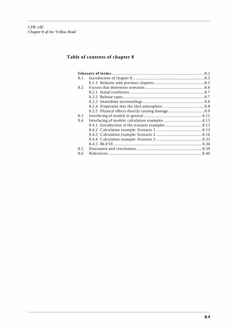
CPR 14EChapter 8 of the ‘Yellow Book’
8.4
Table of contents of chapter 8
Glossary of terms .................................................................................8.28.1 Introduction of chapter 8...............................................................8.5
8.1.1 Relation with previous chapters............................................8.58.2 Factors that determine scenarios ....................................................8.6
8.2.1 Initial conditions .................................................................8.78.2.2 Release types .......................................................................8.78.2.3 Immediate surroundings ......................................................8.88.2.4 Dispersion into the (far) atmosphere ....................................8.88.2.5 Physical effects directly causing damage................................8.9
8.3 Interfacing of models in general ...................................................8.118.4 Interfacing of models: calculation examples ..................................8.13
8.4.1 Introduction of the scenario examples ................................8.138.4.2 Calculation example: Scenario 1 ........................................8.138.4.3 Calculation example: Scenario 2 ........................................8.168.4.4 Calculation example: Scenario 3 ........................................8.338.4.5 BLEVE .............................................................................8.36
8.5 Discussion and conclusions .........................................................8.398.6 References ..................................................................................8.40

CPR 14EChapter 8 of the ‘Yellow Book’
8.5
8.1 Introduction of chapter 8
Safety and risk assessment studies are used to evaluate the risk of activitiesinvolving hazardous materials. The assessment of the hazards requires knowledge ofthe danger each hazardous material could present to human beings and to properties,qualitatively and quantitatively, due to explosion, intoxication, and fires.
In the previous chapters the physical effects related to hazardous materials have beenaddressed independently. Due to the way scientific research is organised most modelshave been developed to describe an isolated specific physical and/or chemicalphenomenon. Where in reality transitions go fluently from one stage to the followingstage of the event that starts with the release of hazardous material and ends with theexposure to people and properties, the modelling of the complete process takes oftenplace stepwise. Most of the time more than one model is needed. These models have to be ‘coupled’,meaning that their results, i.e. the predictions of the models (output data) have to beadapted and transferred to serve as input to other subsequent models. Thus, a particular scenario is represented by a chain of models.The procedure of adaptation and transfer of data is usually addressed by ‘interfacing’.
In this final chapter the interfacing of models will be treated in a general way, and theinterfacing will be put into perspective of so-called scenarios.
The line between the physical effect models to vulnerability or consequence modelsthat estimate the damage to people and properties, will be drawn.
This chapter of the Yellow Book will comprise the following. First, a systematicapproach will be explained regarding how to compile a list with accident scenarios inprinciple. Secondly, ‘interfacing methods’ between similar effect models will beaddressed in general. Next, representative scenarios will be given, that will be workedout numerically as calculation examples.
8.1.1 Relation with previous chapters
Chapter 4 ‘Vapour Cloud Dispersion’ is more or less the central chapter ofthe Yellow Book. This chapter has no special paragraph about interfacing. Interfacingof models into dispersion models are treated in the chapters: Outflow & SprayRelease, Pool Evaporation, Vapour Cloud Explosions.
For the description of other interfacing to models, logical backward chaining has beenfollowed: one has to find required input data from models in prior chapters.
Release of hazardous material, spray release, due to rupture of containments, pipebreaks or cracks in vessels or pipe walls, are initiating events. Therefore, no links ofthe models described in chapter 2 ‘Outflow and Spray Release’ to prior models exist. Vessel rupture is also an initiating event. Therefore no links to prior models exist. The description of the resulting blast effects and fragmentation in chapter 7 ‘Ruptureof Vessels’ is sufficient.

CPR 14EChapter 8 of the ‘Yellow Book’
8.6
8.2 Factors that determine scenarios
The way in which a hazardous material can lead to consequences variesenormously.The processes involved depend on the properties of hazardous material, the processor system conditions, the way in which the accidental decontainment takes place, andpossible subsequent reactions with the environment. A hazardous material can betoxic, flammable or both. The containment may be slightly damaged or totallyruptured by some kind of mechanical impact, or by being set on fire. Released into the atmosphere, the hazardous material may:– cause fire and/or explosions, – lead to atmospheric concentrations of toxic materials to which humans can be
exposed, causing immediate toxic effects,– lead to pollution of the environment.
In order to cope with the wide variety of possible accident developments, the conceptof ‘(accident) scenario’ is used.
In the following a rather restricted definition of scenario is used:
A(n) (accident) scenario is a qualitative description of a particular route by which a(released) hazardous material can lead to one type of physical effect having consequences forhuman beings and or properties.
In order to identify possible scenarios involving hazardous materials, a formal andsomewhat schematic but systematic approach has been chosen: first, the factors areidentified that determine a scenario, secondly, possible realistic scenarios areidentified by combining the possible ‘values’ of these factors.
In general, a scenario is determined by the following factors:
A1. Chemical composition : single compound, mixtureA2. Initial process condition : pressure, temperatureB. Release type : small opening, total ruptureC. Immediate surroundings : mechanical/chemical interaction D. Dispersion : atmospheric dispersion, dispersion in water bodies
or in the groundE. Physical effect : heat flux, blast, atmospheric concentrations of
hazardous materials
These factors will be elucidated in the following sections.

CPR 14EChapter 8 of the ‘Yellow Book’
8.7
8.2.1 Initial conditions
Given the chemical composition of the hazardous material, (partial)pressure and temperature determine the aggregation state of the compound. TheYellow Book deals with gases or vapours and liquids only, thus, the following processconditions are considered:1. compressed gas,2. refrigerated (liquefied) gases,3. non-boiling liquids,4. pressurised liquefied gases
These process conditions determine to a large extend the physical phenomena thatwill occur during the release of the material. An overview is given in the table below.These topics have been addressed in detail in chapters 2 and 3.
Table 8.1 Overview of physical phenomena during the release of material
8.2.2 Release types
The following release types are considered:1. finite duration release,2. instantaneous release.
Ad 1.The containment may be damaged partially, resulting in an opening to theenvironment which is relatively small compared to the total amount of hazardousmaterial in the process. This opening could be a hole in the wall of the containment,or a rupture of a pipe: relatively short piping in installations or relatively longtransport pipelines.
Ad 2.A containment can rupture totally. This causes the content, at least the larger part ofthe inventory, to be released into the environment in a relatively short time.
These topics have been addressed in detail in chapter 2.
Process condition Pre-dispersion effects
Compressed gas (sub-)Sonic release into the atmosphere
Refrigerated gases Pool formation, initially boiling and later on non-boiling evaporating
Non-boiling liquids Pool formation, evaporating but non-boiling
Pressurised liquefied gases Flash off,possibly followed by (immediate) evaporation of a liquid spray due to entrainment of atmospheric air; (partial) rain-out may lead to pool formation and subsequent pool evaporation

CPR 14EChapter 8 of the ‘Yellow Book’
8.8
8.2.3 Immediate surroundings
Depending on the process conditions, the released gas or liquid will interactwith the immediate surroundings. These interactions have a direct effect on the(thermodynamic) state of the hazardous material entraining into the atmosphere.Near the source the dispersion is often still dominated by the effects of the releaseitself. Liquids may spread over land or water (floating) or sink or solve into the subsoil orinto water.
The mechanical interactions influencing the way the entrainment into the atmosphere(atmosphere, water body, or subsoil) takes place, are:1. free entrainment: outflow, jet, spreading,...,2. restricted entrainment: collision with obstacles, bund,... .
Physical-chemical interactions may take place due to a reaction of the hazardousmaterial with the atmosphere (combustion), or with water or subsoil (chemicalreaction).It is also conceivable that a sudden change in physical conditions of releasedchemicals results in auto-reactions such as decomposition or polymerisation.Many topics mentioned here have been addressed in chapters 3 and 6.
Table 8.2 Possible interactions with the environmental of the containment of the material released
8.2.4 Dispersion into the (far) atmosphere
In the ‘Yellow Book’ only atmospheric dispersion is considered.
Gases, vapours and liquid sprays may disperse into the atmosphere.
Environmental compartment Possible physical-chemical interaction
1. Interaction with atmosphere 1.1. no chemical reaction1.2. combustion1.3. auto-reaction
2. Interaction with water 2.1. floating2.2. solving2.3. sinking2.4. reaction2.5. auto-reaction
3. Interaction with subsoil 3.1. no chemical reaction3.2. absorption3.3. reaction3.4. auto-reaction

CPR 14EChapter 8 of the ‘Yellow Book’
8.9
8.2.5 Physical effects directly causing damage
The following physical effects can cause damage to people and properties: 1. heat flux,2. blast,3. atmospheric concentrations of hazardous material.
Ad 1. Heat flux is associated with fire. Combustion can occur in all thermodynamic states:solids, liquids and gases, after ignition. Pressurised gas releases may lead to flares orto local fires. Liquid pools may lead to pool fires. Totally ruptured vessels withpressurised flammable gas can lead to fire balls in case of an ignited BLEVE. Thesetopics have been addressed in detail in chapter 6.
Ad 2.Two types of explosions can be distinguished: physical and chemical explosions. Aphysical explosion is a catastrophic rupture of a pressurised gas-filled vessel; thesudden failure of the vessel causes blast in its immediate environment. These topicshave been addressed in detail in chapter 7.
In a chemical explosion a chemical reaction is generating the energy of the resultingblast. Chemical explosions may be subdivided into two classes. First, gases/vapours, liquids and solids may be explosive by themselves: a rapid auto-reaction causes the blast.Secondly, gases/vapours and liquid sprays may form a flammable mixture with air. After ignition a blast may occur if the flammable gas mixture is (partly) confined byobstacles. These topics have been addressed in detail in chapter 5.
Ad 3.If a released toxic hazardous material is dispersed into the atmosphere, damagingeffects may only be expected due to some kind of physical contact: exposure to theskin, swallowing, inhalation, etc.In the end a release may also result in low concentration pollution of the environment. The topic of atmospheric dispersion has been addressed in detail in chapter 4.
To be able to estimate the expected consequences (damage), besides thecharacteristics of potential targets or receptors (people, properties) the consequencemodels require (basic) input from the physical effect models.
For safety and risk assessment studies this input is the main physical effect parameter ofinterest!
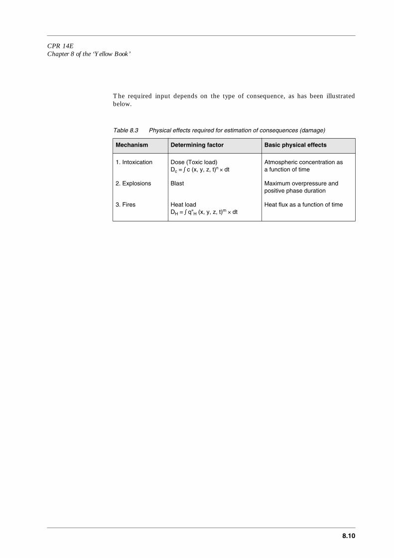
CPR 14EChapter 8 of the ‘Yellow Book’
8.10
The required input depends on the type of consequence, as has been illustratedbelow.
Table 8.3 Physical effects required for estimation of consequences (damage)
Mechanism Determining factor Basic physical effects
1. Intoxication Dose (Toxic load) Dc = ∫ c (x, y, z, t)n × dt
Atmospheric concentration as a function of time
2. Explosions Blast Maximum overpressure and positive phase duration
3. Fires Heat loadDH = ∫ q"H (x, y, z, t)m × dt
Heat flux as a function of time

CPR 14EChapter 8 of the ‘Yellow Book’
8.11
8.3 Interfacing of models in general
Having identified the five factors that determine a scenario, allcombinations of the possible ‘values’ of the factors can be constructed, resulting in alist of possible scenarios. Afterwards, a screening has to be carried out to sort out allcombinations that are physically unrealistic.
In this final chapter we will treat the interfacing of models in a general way, and theinterfacing is put into the perspective of so-called scenarios.
In order to avoid duplications, the interfacing in the perspective of the scenarios ispresented here on a higher abstraction level.The scheme below shows all possible links between the steps within a scenario on ahigher level: links between groups of models.
Table 8.4 Possible steps between groups of models within a scenario
Note that for intoxication the prediction of the concentrations by an atmosphericdispersion model suffices.
This means that the interfacing between the following group of models has to beaddressed.
gases or spray release
– dispersion – (VCE) blast
gas release – heat flux from fire
liquid release orspray release
– evaporation – dispersion – (explosion) blast
liquid release – heat flux from fire
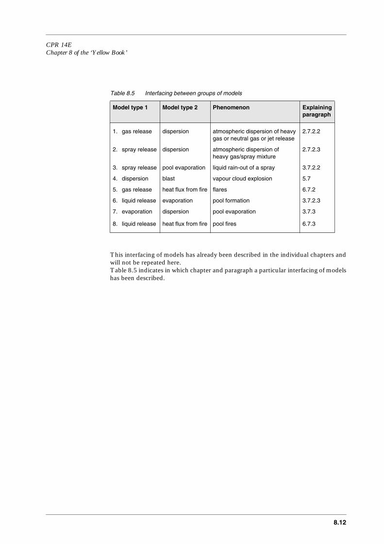
CPR 14EChapter 8 of the ‘Yellow Book’
8.12
Table 8.5 Interfacing between groups of models
This interfacing of models has already been described in the individual chapters andwill not be repeated here.Table 8.5 indicates in which chapter and paragraph a particular interfacing of modelshas been described.
Model type 1 Model type 2 Phenomenon Explainingparagraph
1. gas release dispersion atmospheric dispersion of heavy gas or neutral gas or jet release
2.7.2.2
2. spray release dispersion atmospheric dispersion ofheavy gas/spray mixture
2.7.2.3
3. spray release pool evaporation liquid rain-out of a spray 3.7.2.2
4. dispersion blast vapour cloud explosion 5.7
5. gas release heat flux from fire flares 6.7.2
6. liquid release evaporation pool formation 3.7.2.3
7. evaporation dispersion pool evaporation 3.7.3
8. liquid release heat flux from fire pool fires 6.7.3

CPR 14EChapter 8 of the ‘Yellow Book’
8.13
8.4 Interfacing of models: calculation examples
8.4.1 Introduction of the scenario examples
The following scenarios are more or less illustrative and will be worked outas calculation examples in the following paragraphs.
The scenario descriptions below are expressed as much as possible in terms ofcombinations of ‘values’ of the scenario factors presented previously:
1. The hazardous material is a compressed gas, a hole in its containment permitsrelease to the atmosphere freely, the flammable gas jet is immediately ignited andforms a flare, causing heat flux at some distance;
2. The hazardous material is a refrigerated gas stored under atmospheric pressure,and through a leak in the container liquid is being released freely, so a spreadingboiling floating pool on water will be formed, and evaporation leads toatmospheric concentrations of hazardous material;
3. The hazardous material is a pressurized liquefied gas; a full bore pipe rupturepermits release to the atmosphere, followed by evaporation of a liquid spray dueto mixing with atmospheric air; between obstacles the flammable gas is ignitedafter a delay and an explosion or deflagration may occur;
The physical phenomena related to a BLEVE have been treated in different chapters.In order to give an overall picture of the BLEVE, an integral calculation example willbe given here, so:
4. A BLEVE (Boiling Liquid Expanding Vapour Explosion) shows the followingphysical effects able to cause damage: heat radiation, pressure waves andfragmentation.
No intermediate results of the models will be presented in this chapter, except for theGASP model. Here we merely take the opportunity to demonstrate the capabilities ofthis model.
8.4.2 Calculation example: Scenario 1
Concise scenario description
Compressed methane (CH4) is released from a vessel through a pipe and afterignition a flare results.The (maximum) heat load at maximum outflow rate of methane, and the heat loadat average outflow rate of methane gas will be estimated at several distances to thevessel.
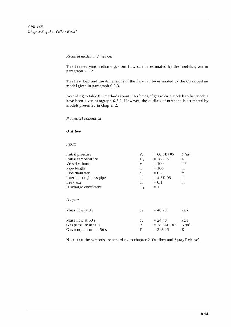
CPR 14EChapter 8 of the ‘Yellow Book’
8.14
Required models and methods
The time-varying methane gas out flow can be estimated by the models given inparagraph 2.5.2.
The heat load and the dimensions of the flare can be estimated by the Chamberlainmodel given in paragraph 6.5.3.
According to table 8.5 methods about interfacing of gas release models to fire modelshave been given paragraph 6.7.2. However, the outflow of methane is estimated bymodels presented in chapter 2.
Numerical elaboration
Outflow
Input:
Initial pressure P0 = 60.0E+05 N/m2
Initial temperature T0 = 288.15 KVessel volume V = 100 m3
Pipe length lp = 100 mPipe diameter dp = 0.2 mInternal roughness pipe ε = 4.5E-05 mLeak size dh = 0.1 mDischarge coefficient Cd = 1
Output:
Mass flow at 0 s qS = 46.29 kg/s
Mass flow at 50 s qS = 24.40 kg/sGas pressure at 50 s P = 28.66E+05 N/m2
Gas temperature at 50 s T = 243.13 K
Note, that the symbols are according to chapter 2 ‘Outflow and Spray Release’.
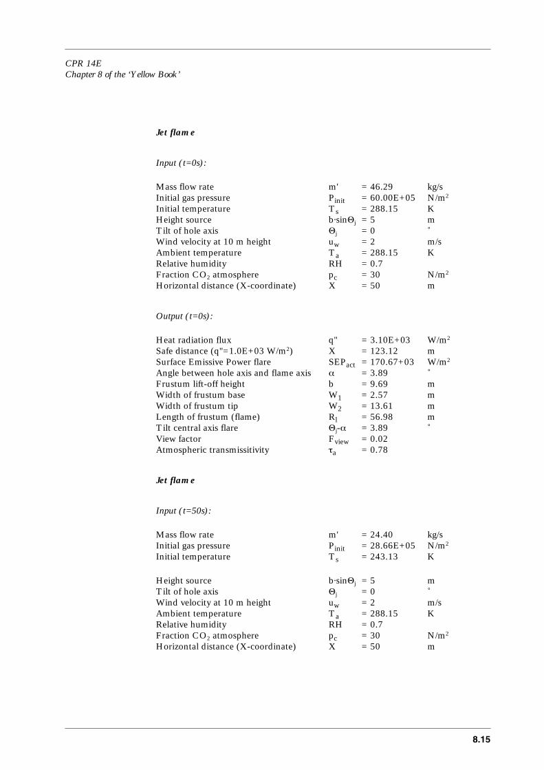
CPR 14EChapter 8 of the ‘Yellow Book’
8.15
Jet flame
Input (t=0s):
Mass flow rate m' = 46.29 kg/sInitial gas pressure Pinit = 60.00E+05 N/m2
Initial temperature Ts = 288.15 KHeight source b⋅sinΘj = 5 mTilt of hole axis Θj = 0 ˚Wind velocity at 10 m height uw = 2 m/sAmbient temperature Ta = 288.15 KRelative humidity RH = 0.7Fraction CO2 atmosphere pc = 30 N/m2
Horizontal distance (X-coordinate) X = 50 m
Output (t=0s):
Heat radiation flux q" = 3.10E+03 W/m2
Safe distance (q"=1.0E+03 W/m2) X = 123.12 mSurface Emissive Power flare SEPact = 170.67+03 W/m2
Angle between hole axis and flame axis α = 3.89 ˚Frustum lift-off height b = 9.69 mWidth of frustum base W1 = 2.57 mWidth of frustum tip W2 = 13.61 mLength of frustum (flame) Rl = 56.98 mTilt central axis flare Θj-α = 3.89 ˚View factor Fview = 0.02Atmospheric transmissitivity τa = 0.78
Jet flame
Input (t=50s):
Mass flow rate m' = 24.40 kg/sInitial gas pressure Pinit = 28.66E+05 N/m2
Initial temperature Ts = 243.13 K
Height source b⋅sinΘj = 5 mTilt of hole axis Θj = 0 ˚Wind velocity at 10 m height uw = 2 m/sAmbient temperature Ta = 288.15 KRelative humidity RH = 0.7Fraction CO2 atmosphere pc = 30 N/m2
Horizontal distance (X-coordinate) X = 50 m

CPR 14EChapter 8 of the ‘Yellow Book’
8.16
Output (t=50s):
Heat radiation flux q" = 2.38E+03 W/m2
Safe distance (q"=1.0E+03 W/m2) X = 92.63 mSurface Emissive Power flare SEPact = 166.0E+03 W/m2
Angle between hole axis and flame axis α = 4.29 ˚Frustum lift-off height b = 7.52 mWidth of frustum base W1 = 2.14 mWidth of frustum tip W2 = 10.70 mLength of frustum (flame) Rl = 40.20 mTilt central axis flare Θj-α = 4.49 ˚View factor Fview = 0.02Atmospheric transmissitivity τa = 0.78
Note, that the symbols are according to chapter 6 ‘Heat fluxes from fires’.
8.4.3 Calculation example: Scenario 2
Concise scenario description
Refrigerated ammonia (NH3), stored in a vertical cylinder, is incidentally releasedthrough a leak in the container wall into the surroundings. A crack occurs in the wallof a pipeline connected to the storage. The cross-sectional area of the crack is about10% of the cross-sectional area of the pipeline. After three hours the release of ammonia can be stopped.An ammonia liquid pool will spread on the ground and evaporate.Some atmospheric concentrations of ammonia, toxic to humans, will be estimated atseveral distances from the source.
Required models and methods
The time-varying outflow of initially non-boiling ammonia liquid from a vessel can beestimated by the models given in paragraph 2.5.4 of chapter ‘Outflow and Sprayrelease’.
The evaporation of a initially boiling and later on non-boiling ammonia pool on landcan be calculated by the GASP model presented in paragraph 3.5.2 of chapter ‘Poolevaporation’.
Atmospheric concentrations of the toxic (heavy) ammonia gas can be estimated bythe SLAB model presented in paragraph 4.5.5.2 of chapter ‘Vapour clouddispersion’.
According to table 8.5 methods about interfacing of liquid release models to poolevaporation models have been given in paragraph 3.7.2.3, and about interfacing ofpool evaporation models to dispersion models in paragraph 3.7.3.

CPR 14EChapter 8 of the ‘Yellow Book’
8.17
Numerical elaboration
Outflow
Input:
Vessel volume V = 30000 m3
Length cylinder hv = 30 mFilling degree φ = 0.75Pressure above liquid P = 101325 N/m2
Pipe length lp = 1 mPipe diameter dp = 0.4 mInternal roughness pipe ε = 4.5⋅10-5 mLeak size dh = 0.1265 mHeight leak hh = 0 mInitial temperature T0 = 237.3 KDischarge coefficient Cd = 1Time after start release t = 10800 s
Output:
Outflow rate liquid at t=0 s qS = 180.59 kg/sat t=3600 s qS = 176.70 kg/sat t=7200 s qS = 172.81 kg/sat t=10800 s qS = 168.92 kg/s
Average outflow rate until t=10800 s qS,av = 174.8 kg/s (0.255 m3/s)Liquid density ρL = 684.4 kg/m3
Filling degree at 10800 s φ = 0.66Height of liquid at 10800 s hL = 19.69 mTotal mass released at 10800 s Q = 0.1926⋅107 kg
Note that the symbols are according to chapter 2 ‘Outflow and Spray release’.
Pool evaporation
GASP models a semi-continuous release of refrigerated ammonia onto land.Ammonia is spilt at a rate of 0.255 m3/s through an aperture of 0.0126 m2. Theimplied discharge velocity is 20.3 m/s.The temperature at the discharge point is 239.72 K.The pool spread is unrestricted. Heat is being transferred from light concrete subsoil,with conductivity 0.418 J(m⋅s⋅K) and diffusivity 2.5 m2/s, into the pool. Perfectthermal contact is assumed. The capillary depth has been set equal to the averageroughness of the light concrete subsoil.The atmospheric temperature is 15 ˚C (288.15 K) and the windspeed is 4.5 m/s.The net solar radiation can be estimated by equations (4.36) and (4.37) presented inchapter 4 ‘Vapour cloud dispersion’. However, for the sake of simplicity a value of100 J/(m2⋅s) for the net solar radiation has been used.
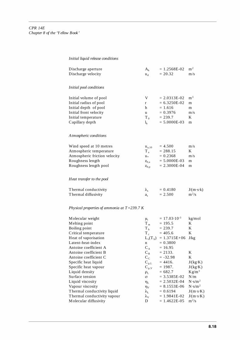
CPR 14EChapter 8 of the ‘Yellow Book’
8.18
Initial liquid release conditions
Discharge aperture Ah = 1.2568E-02 m2
Discharge velocity ud = 20.32 m/s
Initial pool conditions
Initial volume of pool V = 2.0313E-02 m3
Initial radius of pool r = 6.3250E-02 mInitial depth of pool h = 1.616 mInitial front velocity u = 0.3976 m/sInitial temperature T0 = 239.7 KCapillary depth lh = 5.0000E-03 m
Atmospheric conditions
Wind speed at 10 metres ua,10 = 4.500 m/sAtmospheric temperature Ta = 288.15 KAtmospheric friction velocity u* = 0.2368 m/sRoughness length z0,a = 5.0000E-03 mRoughness length pool z0,p = 2.3000E-04 m
Heat transfer to the pool
Thermal conductivity λs = 0.4180 J/(m⋅s⋅k)Thermal diffusivity as = 2.500 m2/s
Physical properties of ammonia at T=239.7 K
Molecular weight µi = 17.03⋅10-3 kg/molMelting point Tm = 195.5 K Boiling point Tb = 239.7 K Critical temperature Tc = 405.6 K Heat of vaporisation Lv(Tb) = 1.3715E+06 J/kg Latent-heat-index n = 0.3800Antoine coefficient A CA = 16.95Antoine coefficient B CB = 2133. K Antoine coefficient C CC = -32.98 K Specific heat liquid Cp,L = 4416. J/(kg⋅K)Specific heat vapour Cp,V = 1987. J/(kg⋅K)Liquid density ρL = 682.7 Kg/m3 Surface tension σ = 3.5385E-02 N/mLiquid viscosity ηL = 2.5032E-04 N⋅s/m2 Vapour viscosity ηV = 8.1553E-06 N⋅s/m2
Thermal conductivity liquid λL = 0.6194 J/(m⋅s⋅K)Thermal conductivity vapour λV = 1.9841E-02 J/(m⋅s⋅K)Molecular diffusivity D = 1.4622E-05 m2/s

CPR 14EChapter 8 of the ‘Yellow Book’
8.19
Properties of air
Density ρa = 1.225 kg/m3
Viscosity ηa = 1.7894E-05 N⋅s/m2
Kinematic viscosity υa = 1.4607E-05 m2/sPrandtl number Pra = 0.7104Effective molecular weight µa = 28.96⋅10-3 kg/mol
Constants
Turbulent friction parameter Cf = 1.3000E-03Von Karman’s constant κ = 0.4000Turbulent Schmidt number Sct = 0.8500Turbulent Prandtl number Prt = 0.85Laminar Schmidt number Scl = 0.9990
Output
Maximum vaporisation rate qS,max = 174.2 k/s after time t = 1.0800E+04 sPool has evaporated at time t = 1.1342E+04 s
Intermediate results of SLAB can be found at the end of this paragraph.
Note that the symbols are according to chapter 3 ‘Pool evaporation’.
Heavy gas dispersion
From table 8.6 it appears that the pool reaches its maximum radius 31.66 m, att=1377 after the start of the release. After t=11342 s the pool has evaporated. Aftert=10800 s (3 hours) the liquid pool surface will keep its maximum size, but the poolwill partially dry up.
While the pool will have its maximum size for about 87.9% of the time, the sourcedimension for the dispersion model SLAB will be assumed to be equal to maximumsize of the pool, thus:
AS = π⋅rp,max2
= 3150 m2
After t=10800 s (3 hours) about Qv≈1.86+06 kg of ammonia has evaporated. Thisimplies an average evaporation rate:
qs,av =172.2 kg/s
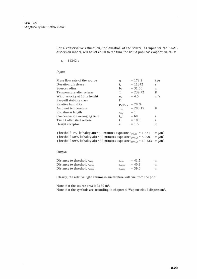
CPR 14EChapter 8 of the ‘Yellow Book’
8.20
For a conservative estimation, the duration of the source, as input for the SLABdispersion model, will be set equal to the time the liquid pool has evaporated, thus:
tS = 11342 s
Input:
Mass flow rate of the source q = 172.2 kg/sDuration of release tr = 11342 sSource radius b0 = 31.66 mTemperature after release T = 239.72 KWind velocity at 10 m height ua = 4.5 m/sPasquill stability class DRelative humidity pw/ps,w = 70 %Ambient temperature Ta = 288.15 KRoughness length z0,p = 1Concentration averaging time tav = 60 sTime t after start release t = 1800 sHeight receptor z = 1.5 m
Threshold 1% lethality after 30 minutes exposure c1%,30 = 1,871 mg/m3
Threshold 50% lethality after 30 minutes exposurec50%,30= 5,999 mg/m3
Threshold 99% lethality after 30 minutes exposurec99%,30= 19,233 mg/m3
Output:
Distance to threshold c1% x1% = 41.5 mDistance to threshold c50% x50% = 40.3 mDistance to threshold c99% x99% = 39.0 m
Clearly, the relative light ammonia-air-mixture will rise from the pool.
Note that the source area is 3150 m2.Note that the symbols are according to chapter 4 ‘Vapour cloud dispersion’.

CPR 14EChapter 8 of the ‘Yellow Book’
8.21
Table 8.6
t(s)
r(m)
Qv(kg)
h(m)
Vd(m3)
0.0000 6.3250E-02 0.0000 1.616 2.0313E-025.0338E-04 6.3469E-02 4.3812E-07 1.615 2.0442E-022.4550E-03 6.4676E-02 2.1707E-06 1.593 2.0940E-026.1352E-03 6.8472E-02 5.6723E-06 1.485 2.1880E-021.1777E-02 7.7885E-02 1.2071E-05 1.224 2.3321E-021.8536E-02 9.3989E-02 2.2489E-05 0.9025 2.5047E-022.7798E-02 0.1223 4.4693E-05 0.5831 2.7413E-023.8736E-02 0.1619 8.9195E-05 0.3669 3.0206E-025.5937E-02 0.2315 2.2189E-04 0.2054 3.4599E-027.6240E-02 0.3198 5.2831E-04 0.1238 3.9784E-029.9749E-02 0.4256 1.1731E-03 8.0461E-02 4.5788E-020.1308 0.5676 2.6759E-03 5.3077E-02 5.3721E-020.1718 0.7545 6.1692E-03 3.5888E-02 6.4191E-020.2273 1.001 1.4464E-02 2.4887E-02 7.8371E-020.3085 1.339 3.5931E-02 1.7585E-02 9.9111E-020.4319 1.789 9.4027E-02 1.2974E-02 0.13060.5909 2.261 0.2186 1.0643E-02 0.17120.7524 2.641 0.4025 9.6679E-03 0.21250.9425 2.999 0.6879 9.2016E-03 0.26101.202 3.384 1.186 9.0513E-03 0.32731.526 3.758 1.961 9.1793E-03 0.41011.875 4.079 2.962 9.4702E-03 0.49932.331 4.417 4.496 9.9360E-03 0.61572.897 4.758 6.708 1.0549E-02 0.76013.615 5.112 9.952 1.1315E-02 0.94354.539 5.488 14.76 1.2237E-02 1.1805.743 5.900 21.96 1.3302E-02 1.4877.382 6.386 33.36 1.4494E-02 1.9069.578 6.977 51.35 1.5637E-02 2.46612.56 7.752 80.99 1.6476E-02 3.22916.67 8.816 132.3 1.6727E-02 4.27821.87 10.13 217.1 1.6396E-02 5.60528.14 11.60 351.3 1.5832E-02 7.20737.08 13.42 603.9 1.5198E-02 9.48948.64 15.41 1036. 1.4650E-02 12.4464.42 17.65 1807. 1.4127E-02 16.4777.84 19.27 2620. 1.3768E-02 19.9097.99 21.35 4094. 1.3305E-02 25.05130.4 24.02 7049. 1.2697E-02 33.33179.2 26.86 1.2632E+04 1.2039E-02 45.79194.2 27.51 1.4568E+04 1.1894E-02 49.61197.8 27.65 1.5050E+04 1.1863E-02 50.54213.6 28.21 1.7207E+04 1.1752E-02 54.58239.2 28.87 2.0852E+04 1.1673E-02 61.11
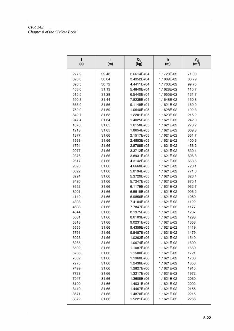
CPR 14EChapter 8 of the ‘Yellow Book’
8.22
277.9 29.48 2.6614E+04 1.1728E-02 71.00328.0 30.04 3.4352E+04 1.1809E-02 83.79390.5 30.72 4.4411E+04 1.1703E-02 99.75453.0 31.13 5.4840E+04 1.1628E-02 115.7515.5 31.28 6.5440E+04 1.1655E-02 131.7590.3 31.44 7.8235E+04 1.1648E-02 150.8665.0 31.56 9.1149E+04 1.1621E-02 169.9752.9 31.59 1.0640E+05 1.1628E-02 192.3842.7 31.63 1.2201E+05 1.1623E-02 215.2947.4 31.64 1.4025E+05 1.1621E-02 242.01070. 31.65 1.6158E+05 1.1621E-02 273.21213. 31.65 1.8654E+05 1.1621E-02 309.81377. 31.66 2.1517E+05 1.1621E-02 351.71568. 31.66 2.4853E+05 1.1621E-02 400.61794. 31.66 2.8788E+05 1.1621E-02 458.22077. 31.66 3.3712E+05 1.1621E-02 530.42376. 31.66 3.8931E+05 1.1621E-02 606.82617. 31.66 4.3142E+05 1.1621E-02 668.52820. 31.66 4.6668E+05 1.1621E-02 720.13022. 31.66 5.0194E+05 1.1621E-02 771.83224. 31.66 5.3720E+05 1.1621E-02 823.43426. 31.66 5.7247E+05 1.1621E-02 875.13652. 31.66 6.1179E+05 1.1621E-02 932.73901. 31.66 6.5518E+05 1.1621E-02 996.24149. 31.66 6.9856E+05 1.1621E-02 1060.4393. 31.66 7.4104E+05 1.1621E-02 1122.4608. 31.66 7.7847E+05 1.1621E-02 1177.4844. 31.66 8.1975E+05 1.1621E-02 1237.5081. 31.66 8.6103E+05 1.1621E-02 1298.5318. 31.66 9.0231E+05 1.1621E-02 1358.5555. 31.66 9.4359E+05 1.1621E-02 1419.5791. 31.66 9.8487E+05 1.1621E-02 1479.6028. 31.66 1.0262E+06 1.1621E-02 1540.6265. 31.66 1.0674E+06 1.1621E-02 1600.6502. 31.66 1.1087E+06 1.1621E-02 1660.6738. 31.66 1.1500E+06 1.1621E-02 1721.7002. 31.66 1.1960E+06 1.1621E-02 1788.7275. 31.66 1.2436E+06 1.1621E-02 1858.7499. 31.66 1.2827E+06 1.1621E-02 1915.7723. 31.66 1.3217E+06 1.1621E-02 1972.7947. 31.66 1.3608E+06 1.1621E-02 2030.8190. 31.66 1.4031E+06 1.1621E-02 2092.8440. 31.66 1.4467E+06 1.1621E-02 2155.8671. 31.66 1.4870E+06 1.1621E-02 2215.8872. 31.66 1.5221E+06 1.1621E-02 2266.
t(s)
r(m)
Qv(kg)
h(m)
Vd(m3)
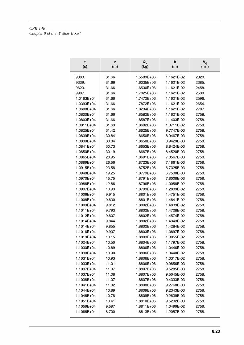
CPR 14EChapter 8 of the ‘Yellow Book’
8.23
9083. 31.66 1.5589E+06 1.1621E-02 2320.9339. 31.66 1.6035E+06 1.1621E-02 2385.9623. 31.66 1.6530E+06 1.1621E-02 2458.9907. 31.66 1.7025E+06 1.1621E-02 2530.1.0163E+04 31.66 1.7472E+06 1.1621E-02 2596.1.0393E+04 31.66 1.7872E+06 1.1621E-02 2654.1.0600E+04 31.66 1.8234E+06 1.1621E-02 2707.1.0800E+04 31.66 1.8582E+06 1.1621E-02 2758.1.0803E+04 31.66 1.8587E+06 1.1403E-02 2758.1.0811E+04 31.63 1.8602E+06 1.0711E-02 2758.1.0825E+04 31.42 1.8625E+06 9.7747E-03 2758.1.0839E+04 30.84 1.8650E+06 8.9467E-03 2758.1.0839E+04 30.84 1.8650E+06 8.9429E-03 2758.1.0841E+04 30.73 1.8653E+06 8.8424E-03 2758.1.0850E+04 30.19 1.8667E+06 8.4520E-03 2758.1.0865E+04 28.95 1.8691E+06 7.8567E-03 2758.1.0889E+04 26.56 1.8723E+06 7.1861E-03 2758.1.0915E+04 23.58 1.8752E+06 6.7325E-03 2758.1.0948E+04 19.25 1.8779E+06 6.7530E-03 2758.1.0970E+04 15.75 1.8791E+06 7.8008E-03 2758.1.0986E+04 12.86 1.8796E+06 1.0058E-02 2758.1.0997E+04 10.93 1.8799E+06 1.2839E-02 2758.1.1006E+04 9.915 1.8801E+06 1.4751E-02 2758.1.1008E+04 9.830 1.8801E+06 1.4841E-02 2758.1.1009E+04 9.812 1.8802E+06 1.4839E-02 2758.1.1011E+04 9.793 1.8802E+06 1.4728E-02 2758.1.1012E+04 9.807 1.8802E+06 1.4574E-02 2758.1.1014E+04 9.844 1.8802E+06 1.4343E-02 2758.1.1014E+04 9.855 1.8802E+06 1.4284E-02 2758.1.1016E+04 9.937 1.8803E+06 1.3897E-02 2758.1.1019E+04 10.15 1.8803E+06 1.3055E-02 2758.1.1024E+04 10.50 1.8804E+06 1.1797E-02 2758.1.1030E+04 10.89 1.8806E+06 1.0446E-02 2758.1.1030E+04 10.90 1.8806E+06 1.0440E-02 2758.1.1031E+04 10.93 1.8806E+06 1.0317E-02 2758.1.1033E+04 11.01 1.8806E+06 9.9856E-03 2758.1.1037E+04 11.07 1.8807E+06 9.5285E-03 2758.1.1037E+04 11.08 1.8807E+06 9.5045E-03 2758.1.1038E+04 11.07 1.8807E+06 9.4333E-03 2758.1.1041E+04 11.02 1.8808E+06 9.2768E-03 2758.1.1044E+04 10.89 1.8809E+06 9.2343E-03 2758.1.1046E+04 10.78 1.8809E+06 9.2639E-03 2758.1.1051E+04 10.41 1.8810E+06 9.5232E-03 2758.1.1059E+04 9.597 1.8811E+06 1.0499E-02 2758.1.1066E+04 8.700 1.8813E+06 1.2057E-02 2758.
t(s)
r(m)
Qv(kg)
h(m)
Vd(m3)

CPR 14EChapter 8 of the ‘Yellow Book’
8.24
1.1072E+04 8.139 1.8813E+06 1.3224E-02 2758.1.1076E+04 7.948 1.8814E+06 1.3552E-02 2758.1.1076E+04 7.938 1.8814E+06 1.3562E-02 2758.1.1078E+04 7.892 1.8814E+06 1.3546E-02 2758.1.1080E+04 7.883 1.8814E+06 1.3453E-02 2758.1.1080E+04 7.884 1.8814E+06 1.3410E-02 2758.1.1082E+04 7.913 1.8815E+06 1.3129E-02 2758.1.1085E+04 7.998 1.8815E+06 1.2614E-02 2758.1.1085E+04 7.999 1.8815E+06 1.2608E-02 2758.1.1086E+04 8.041 1.8815E+06 1.2385E-02 2758.1.1089E+04 8.165 1.8815E+06 1.1776E-02 2758.1.1091E+04 8.258 1.8816E+06 1.1331E-02 2758.1.1092E+04 8.275 1.8816E+06 1.1251E-02 2758.1.1094E+04 8.353 1.8816E+06 1.0865E-02 2758.1.1098E+04 8.451 1.8816E+06 1.0246E-02 2758.1.1100E+04 8.458 1.8817E+06 1.0105E-02 2758.1.1100E+04 8.457 1.8817E+06 1.0055E-02 2758.1.1103E+04 8.419 1.8817E+06 9.9210E-03 2758.1.1106E+04 8.297 1.8818E+06 9.9233E-03 2758.1.1106E+04 8.291 1.8818E+06 9.9271E-03 2758.1.1108E+04 8.199 1.8818E+06 1.0005E-02 2758.1.1112E+04 7.916 1.8818E+06 1.0376E-02 2758.1.1118E+04 7.363 1.8819E+06 1.1413E-02 2758.1.1125E+04 6.855 1.8819E+06 1.2598E-02 2758.1.1129E+04 6.652 1.8820E+06 1.3038E-02 2758.1.1129E+04 6.651 1.8820E+06 1.3039E-02 2758.1.1130E+04 6.602 1.8820E+06 1.3086E-02 2758.1.1133E+04 6.575 1.8820E+06 1.2972E-02 2758.1.1133E+04 6.575 1.8820E+06 1.2963E-02 2758.1.1134E+04 6.582 1.8820E+06 1.2834E-02 2758.1.1137E+04 6.631 1.8820E+06 1.2415E-02 2758.1.1142E+04 6.770 1.8821E+06 1.1525E-02 2758.1.1147E+04 6.902 1.8821E+06 1.0588E-02 2758.1.1150E+04 6.907 1.8822E+06 1.0397E-02 2758.1.1152E+04 6.883 1.8822E+06 1.0294E-02 2758.1.1155E+04 6.756 1.8822E+06 1.0345E-02 2758.1.1157E+04 6.681 1.8822E+06 1.0448E-02 2758.1.1160E+04 6.477 1.8822E+06 1.0823E-02 2758.1.1166E+04 6.060 1.8823E+06 1.1833E-02 2758.1.1172E+04 5.733 1.8823E+06 1.2695E-02 2758.1.1172E+04 5.728 1.8823E+06 1.2706E-02 2758.1.1173E+04 5.694 1.8823E+06 1.2768E-02 2758.1.1176E+04 5.649 1.8823E+06 1.2761E-02 2758.1.1177E+04 5.643 1.8824E+06 1.2692E-02 2758.1.1177E+04 5.644 1.8824E+06 1.2657E-02 2758.
t(s)
r(m)
Qv(kg)
h(m)
Vd(m3)
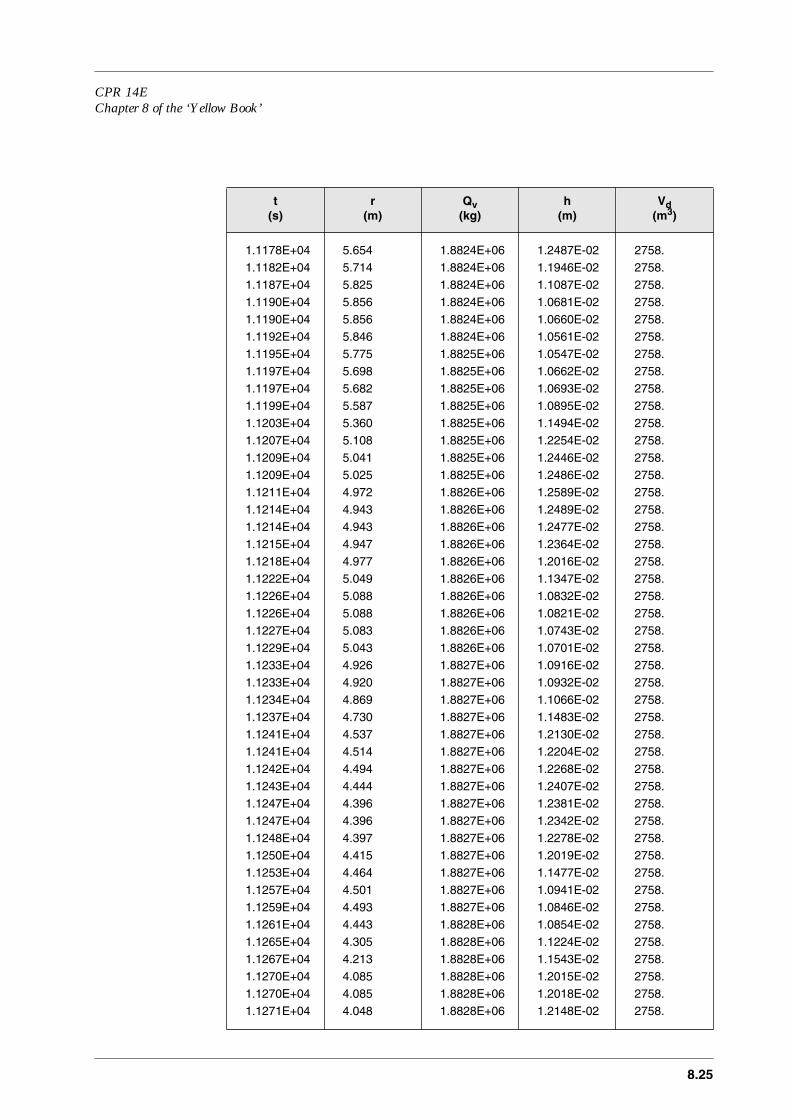
CPR 14EChapter 8 of the ‘Yellow Book’
8.25
1.1178E+04 5.654 1.8824E+06 1.2487E-02 2758.1.1182E+04 5.714 1.8824E+06 1.1946E-02 2758.1.1187E+04 5.825 1.8824E+06 1.1087E-02 2758.1.1190E+04 5.856 1.8824E+06 1.0681E-02 2758.1.1190E+04 5.856 1.8824E+06 1.0660E-02 2758.1.1192E+04 5.846 1.8824E+06 1.0561E-02 2758.1.1195E+04 5.775 1.8825E+06 1.0547E-02 2758.1.1197E+04 5.698 1.8825E+06 1.0662E-02 2758.1.1197E+04 5.682 1.8825E+06 1.0693E-02 2758.1.1199E+04 5.587 1.8825E+06 1.0895E-02 2758.1.1203E+04 5.360 1.8825E+06 1.1494E-02 2758.1.1207E+04 5.108 1.8825E+06 1.2254E-02 2758.1.1209E+04 5.041 1.8825E+06 1.2446E-02 2758.1.1209E+04 5.025 1.8825E+06 1.2486E-02 2758.1.1211E+04 4.972 1.8826E+06 1.2589E-02 2758.1.1214E+04 4.943 1.8826E+06 1.2489E-02 2758.1.1214E+04 4.943 1.8826E+06 1.2477E-02 2758.1.1215E+04 4.947 1.8826E+06 1.2364E-02 2758.1.1218E+04 4.977 1.8826E+06 1.2016E-02 2758.1.1222E+04 5.049 1.8826E+06 1.1347E-02 2758.1.1226E+04 5.088 1.8826E+06 1.0832E-02 2758.1.1226E+04 5.088 1.8826E+06 1.0821E-02 2758.1.1227E+04 5.083 1.8826E+06 1.0743E-02 2758.1.1229E+04 5.043 1.8826E+06 1.0701E-02 2758.1.1233E+04 4.926 1.8827E+06 1.0916E-02 2758.1.1233E+04 4.920 1.8827E+06 1.0932E-02 2758.1.1234E+04 4.869 1.8827E+06 1.1066E-02 2758.1.1237E+04 4.730 1.8827E+06 1.1483E-02 2758.1.1241E+04 4.537 1.8827E+06 1.2130E-02 2758.1.1241E+04 4.514 1.8827E+06 1.2204E-02 2758.1.1242E+04 4.494 1.8827E+06 1.2268E-02 2758.1.1243E+04 4.444 1.8827E+06 1.2407E-02 2758.1.1247E+04 4.396 1.8827E+06 1.2381E-02 2758.1.1247E+04 4.396 1.8827E+06 1.2342E-02 2758.1.1248E+04 4.397 1.8827E+06 1.2278E-02 2758.1.1250E+04 4.415 1.8827E+06 1.2019E-02 2758.1.1253E+04 4.464 1.8827E+06 1.1477E-02 2758.1.1257E+04 4.501 1.8827E+06 1.0941E-02 2758.1.1259E+04 4.493 1.8827E+06 1.0846E-02 2758.1.1261E+04 4.443 1.8828E+06 1.0854E-02 2758.1.1265E+04 4.305 1.8828E+06 1.1224E-02 2758.1.1267E+04 4.213 1.8828E+06 1.1543E-02 2758.1.1270E+04 4.085 1.8828E+06 1.2015E-02 2758.1.1270E+04 4.085 1.8828E+06 1.2018E-02 2758.1.1271E+04 4.048 1.8828E+06 1.2148E-02 2758.
t(s)
r(m)
Qv(kg)
h(m)
Vd(m3)

CPR 14EChapter 8 of the ‘Yellow Book’
8.26
1.1273E+04 3.988 1.8828E+06 1.2330E-02 2758.1.1276E+04 3.956 1.8828E+06 1.2263E-02 2758.1.1276E+04 3.956 1.8828E+06 1.2261E-02 2758.1.1277E+04 3.957 1.8828E+06 1.2179E-02 2758.1.1279E+04 3.974 1.8828E+06 1.1907E-02 2758.1.1282E+04 4.018 1.8828E+06 1.1365E-02 2758.1.1286E+04 4.035 1.8828E+06 1.0985E-02 2758.1.1287E+04 4.020 1.8828E+06 1.0914E-02 2758.1.1291E+04 3.936 1.8829E+06 1.1082E-02 2758.1.1295E+04 3.768 1.8829E+06 1.1704E-02 2758.1.1295E+04 3.767 1.8829E+06 1.1709E-02 2758.1.1296E+04 3.739 1.8829E+06 1.1826E-02 2758.1.1298E+04 3.672 1.8829E+06 1.2093E-02 2758.1.1301E+04 3.603 1.8829E+06 1.2279E-02 2758.1.1303E+04 3.594 1.8829E+06 1.2185E-02 2758.1.1303E+04 3.594 1.8829E+06 1.2160E-02 2758.1.1304E+04 3.601 1.8829E+06 1.2003E-02 2758.1.1307E+04 3.627 1.8829E+06 1.1621E-02 2758.1.1310E+04 3.658 1.8829E+06 1.1136E-02 2758.1.1310E+04 3.658 1.8829E+06 1.1084E-02 2758.1.1311E+04 3.658 1.8829E+06 1.1041E-02 2758.1.1313E+04 3.642 1.8829E+06 1.0980E-02 2758.1.1316E+04 3.569 1.8829E+06 1.1161E-02 2758.1.1320E+04 3.415 1.8829E+06 1.1805E-02 2758.1.1325E+04 3.298 1.8829E+06 1.2229E-02 2758.1.1326E+04 3.291 1.8829E+06 1.2143E-02 2758.1.1327E+04 3.291 1.8829E+06 1.2118E-02 2758.1.1328E+04 3.298 1.8829E+06 1.1947E-02 2758.1.1330E+04 3.323 1.8829E+06 1.1565E-02 2758.1.1334E+04 3.346 1.8830E+06 1.1125E-02 2758.1.1334E+04 3.346 1.8830E+06 1.1124E-02 2758.1.1334E+04 3.345 1.8830E+06 1.1077E-02 2758.1.1336E+04 3.333 1.8830E+06 1.1027E-02 2758.1.1339E+04 3.263 1.8830E+06 1.1227E-02 2758.1.1342E+04 3.146 1.8830E+06 1.1763E-02 2758.
t(s)
r(m)
Qv(kg)
h(m)
Vd(m3)

CPR 14EChapter 8 of the ‘Yellow Book’
8.27
Table 8.8
t(s)
Hc(J(m2⋅s))
Ha(J/(m2⋅s))
T(K)
0.0000 1.9457E+05 0.4159 239.75.0338E-04 465.8 0.4161 239.72.4550E-03 406.0 0.4172 239.76.1352E-03 379.6 0.4205 239.71.1777E-02 334.0 0.4272 239.71.8536E-02 278.6 0.4358 239.72.7798E-02 217.4 0.4455 239.73.8736E-02 168.6 0.4534 239.75.5937E-02 124.0 0.4655 239.77.6240E-02 95.87 0.4742 239.79.9749E-02 77.57 0.4778 239.70.1308 63.51 0.4794 239.70.1718 52.57 0.4796 239.70.2273 43.64 0.4788 239.70.3085 35.70 0.4771 239.70.4319 28.47 0.4747 239.70.5909 22.91 0.4735 239.70.7524 19.34 0.4724 239.70.9425 16.56 0.4714 239.71.202 14.07 0.4703 239.71.526 12.08 0.4690 239.71.875 10.66 0.4679 239.72.331 9.404 0.4668 239.72.897 8.355 0.4658 239.73.615 7.456 0.4648 239.74.539 6.681 0.4637 239.75.743 6.011 0.4626 239.77.382 5.415 0.4614 239.79.578 4.900 0.4601 239.712.56 4.440 0.4584 239.716.67 4.002 0.4563 239.721.87 3.581 0.4540 239.728.14 3.181 0.4518 239.737.08 2.761 0.4493 239.748.64 2.389 0.4469 239.764.42 2.059 0.4445 239.777.84 1.864 0.4431 239.797.99 1.652 0.4414 239.7130.4 1.421 0.4395 239.7179.2 1.202 0.4376 239.7194.2 1.153 0.4372 239.7197.8 1.143 0.4371 239.7213.6 1.098 0.4368 239.7239.2 1.037 0.4364 239.7
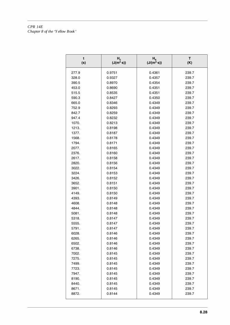
CPR 14EChapter 8 of the ‘Yellow Book’
8.28
277.9 0.9751 0.4361 239.7328.0 0.9327 0.4357 239.7390.5 0.8970 0.4354 239.7453.0 0.8690 0.4351 239.7515.5 0.8535 0.4351 239.7590.3 0.8427 0.4350 239.7665.0 0.8346 0.4349 239.7752.9 0.8293 0.4349 239.7842.7 0.8259 0.4349 239.7947.4 0.8232 0.4349 239.71070. 0.8213 0.4349 239.71213. 0.8198 0.4349 239.71377. 0.8187 0.4349 239.71568. 0.8178 0.4349 239.71794. 0.8171 0.4349 239.72077. 0.8165 0.4349 239.72376. 0.8160 0.4349 239.72617. 0.8158 0.4349 239.72820. 0.8156 0.4349 239.73022. 0.8154 0.4349 239.73224. 0.8153 0.4349 239.73426. 0.8152 0.4349 239.73652. 0.8151 0.4349 239.73901. 0.8150 0.4349 239.74149. 0.8150 0.4349 239.74393. 0.8149 0.4349 239.74608. 0.8148 0.4349 239.74844. 0.8148 0.4349 239.75081. 0.8148 0.4349 239.75318. 0.8147 0.4349 239.75555. 0.8147 0.4349 239.75791. 0.8147 0.4349 239.76028. 0.8146 0.4349 239.76265. 0.8146 0.4349 239.76502. 0.8146 0.4349 239.76738. 0.8146 0.4349 239.77002. 0.8145 0.4349 239.77275. 0.8145 0.4349 239.77499. 0.8145 0.4349 239.77723. 0.8145 0.4349 239.77947. 0.8145 0.4349 239.78190. 0.8145 0.4349 239.78440. 0.8145 0.4349 239.78671. 0.8145 0.4349 239.78872. 0.8144 0.4349 239.7
t(s)
Hc(J(m2⋅s))
Ha(J/(m2⋅s))
T(K)

CPR 14EChapter 8 of the ‘Yellow Book’
8.29
9083. 0.8144 0.4349 239.79339. 0.8144 0.4349 239.79623. 0.8144 0.4349 239.79907. 0.8144 0.4349 239.71.0163E+04 0.8144 0.4349 239.71.0393E+04 0.8144 0.4349 239.71.0600E+04 0.8144 0.4349 239.71.0800E+04 0.8144 0.4349 239.71.0803E+04 0.8144 0.4349 239.71.0811E+04 0.8150 0.4349 239.71.0825E+04 0.8203 0.4350 239.71.0839E+04 0.8351 0.4353 239.71.0839E+04 0.8352 0.4353 239.71.0841E+04 0.8378 0.4354 239.71.0850E+04 0.8491 0.4357 239.71.0865E+04 0.8636 0.4364 239.71.0889E+04 0.8096 0.4378 239.71.0915E+04 -.7068 0.4398 239.71.0948E+04 -1.944 0.4431 239.71.0970E+04 -3.357 0.4465 239.71.0986E+04 -5.304 0.4500 239.71.0997E+04 -7.162 0.4528 239.71.1006E+04 -7.883 0.4544 239.71.1008E+04 -7.769 0.4545 239.71.1009E+04 -7.708 0.4546 239.71.1011E+04 -7.450 0.4546 239.71.1012E+04 -7.233 0.4546 239.71.1014E+04 -6.962 0.4545 239.71.1014E+04 -6.899 0.4545 239.71.1016E+04 -6.518 0.4544 239.71.1019E+04 -5.801 0.4540 239.71.1024E+04 -4.907 0.4534 239.71.1030E+04 -4.166 0.4528 239.71.1030E+04 -4.164 0.4528 239.71.1031E+04 -4.112 0.4528 239.71.1033E+04 -3.994 0.4527 239.71.1037E+04 -3.928 0.4526 239.71.1037E+04 -3.931 0.4526 239.71.1038E+04 -3.945 0.4526 239.71.1041E+04 -4.056 0.4526 239.71.1044E+04 -4.270 0.4528 239.71.1046E+04 -4.435 0.4530 239.71.1051E+04 -4.992 0.4536 239.71.1059E+04 -6.257 0.4549 239.71.1066E+04 -7.792 0.4565 239.7
t(s)
Hc(J(m2⋅s))
Ha(J/(m2⋅s))
T(K)
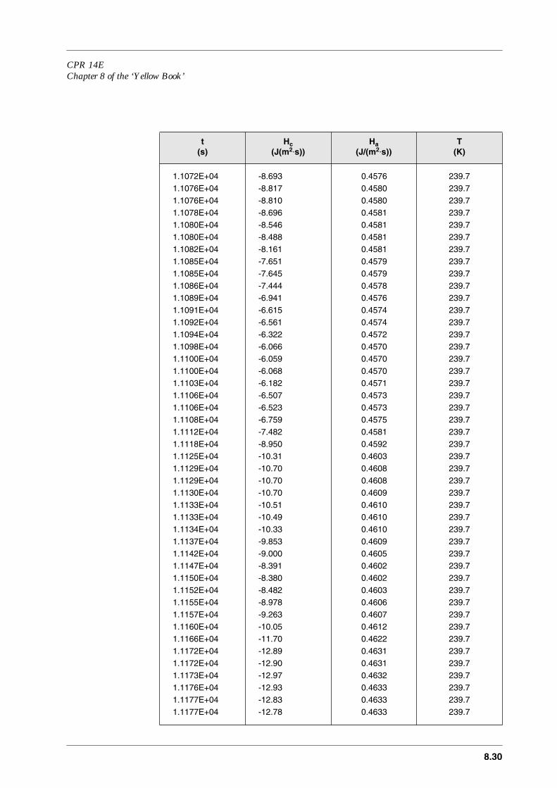
CPR 14EChapter 8 of the ‘Yellow Book’
8.30
1.1072E+04 -8.693 0.4576 239.71.1076E+04 -8.817 0.4580 239.71.1076E+04 -8.810 0.4580 239.71.1078E+04 -8.696 0.4581 239.71.1080E+04 -8.546 0.4581 239.71.1080E+04 -8.488 0.4581 239.71.1082E+04 -8.161 0.4581 239.71.1085E+04 -7.651 0.4579 239.71.1085E+04 -7.645 0.4579 239.71.1086E+04 -7.444 0.4578 239.71.1089E+04 -6.941 0.4576 239.71.1091E+04 -6.615 0.4574 239.71.1092E+04 -6.561 0.4574 239.71.1094E+04 -6.322 0.4572 239.71.1098E+04 -6.066 0.4570 239.71.1100E+04 -6.059 0.4570 239.71.1100E+04 -6.068 0.4570 239.71.1103E+04 -6.182 0.4571 239.71.1106E+04 -6.507 0.4573 239.71.1106E+04 -6.523 0.4573 239.71.1108E+04 -6.759 0.4575 239.71.1112E+04 -7.482 0.4581 239.71.1118E+04 -8.950 0.4592 239.71.1125E+04 -10.31 0.4603 239.71.1129E+04 -10.70 0.4608 239.71.1129E+04 -10.70 0.4608 239.71.1130E+04 -10.70 0.4609 239.71.1133E+04 -10.51 0.4610 239.71.1133E+04 -10.49 0.4610 239.71.1134E+04 -10.33 0.4610 239.71.1137E+04 -9.853 0.4609 239.71.1142E+04 -9.000 0.4605 239.71.1147E+04 -8.391 0.4602 239.71.1150E+04 -8.380 0.4602 239.71.1152E+04 -8.482 0.4603 239.71.1155E+04 -8.978 0.4606 239.71.1157E+04 -9.263 0.4607 239.71.1160E+04 -10.05 0.4612 239.71.1166E+04 -11.70 0.4622 239.71.1172E+04 -12.89 0.4631 239.71.1172E+04 -12.90 0.4631 239.71.1173E+04 -12.97 0.4632 239.71.1176E+04 -12.93 0.4633 239.71.1177E+04 -12.83 0.4633 239.71.1177E+04 -12.78 0.4633 239.7
t(s)
Hc(J(m2⋅s))
Ha(J/(m2⋅s))
T(K)
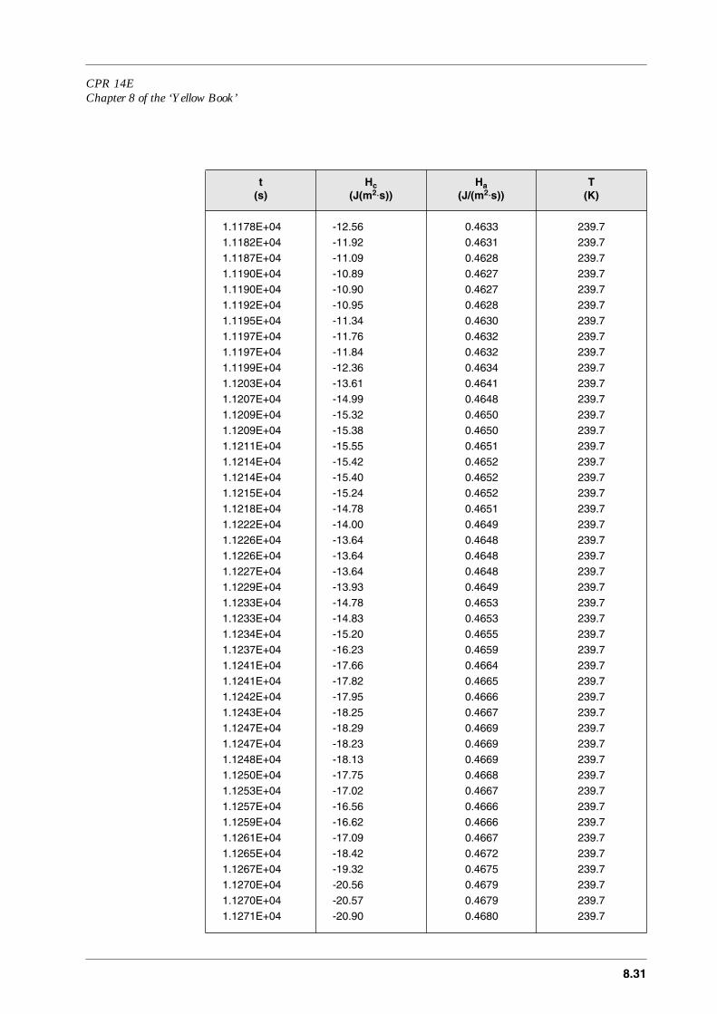
CPR 14EChapter 8 of the ‘Yellow Book’
8.31
1.1178E+04 -12.56 0.4633 239.71.1182E+04 -11.92 0.4631 239.71.1187E+04 -11.09 0.4628 239.71.1190E+04 -10.89 0.4627 239.71.1190E+04 -10.90 0.4627 239.71.1192E+04 -10.95 0.4628 239.71.1195E+04 -11.34 0.4630 239.71.1197E+04 -11.76 0.4632 239.71.1197E+04 -11.84 0.4632 239.71.1199E+04 -12.36 0.4634 239.71.1203E+04 -13.61 0.4641 239.71.1207E+04 -14.99 0.4648 239.71.1209E+04 -15.32 0.4650 239.71.1209E+04 -15.38 0.4650 239.71.1211E+04 -15.55 0.4651 239.71.1214E+04 -15.42 0.4652 239.71.1214E+04 -15.40 0.4652 239.71.1215E+04 -15.24 0.4652 239.71.1218E+04 -14.78 0.4651 239.71.1222E+04 -14.00 0.4649 239.71.1226E+04 -13.64 0.4648 239.71.1226E+04 -13.64 0.4648 239.71.1227E+04 -13.64 0.4648 239.71.1229E+04 -13.93 0.4649 239.71.1233E+04 -14.78 0.4653 239.71.1233E+04 -14.83 0.4653 239.71.1234E+04 -15.20 0.4655 239.71.1237E+04 -16.23 0.4659 239.71.1241E+04 -17.66 0.4664 239.71.1241E+04 -17.82 0.4665 239.71.1242E+04 -17.95 0.4666 239.71.1243E+04 -18.25 0.4667 239.71.1247E+04 -18.29 0.4669 239.71.1247E+04 -18.23 0.4669 239.71.1248E+04 -18.13 0.4669 239.71.1250E+04 -17.75 0.4668 239.71.1253E+04 -17.02 0.4667 239.71.1257E+04 -16.56 0.4666 239.71.1259E+04 -16.62 0.4666 239.71.1261E+04 -17.09 0.4667 239.71.1265E+04 -18.42 0.4672 239.71.1267E+04 -19.32 0.4675 239.71.1270E+04 -20.56 0.4679 239.71.1270E+04 -20.57 0.4679 239.71.1271E+04 -20.90 0.4680 239.7
t(s)
Hc(J(m2⋅s))
Ha(J/(m2⋅s))
T(K)
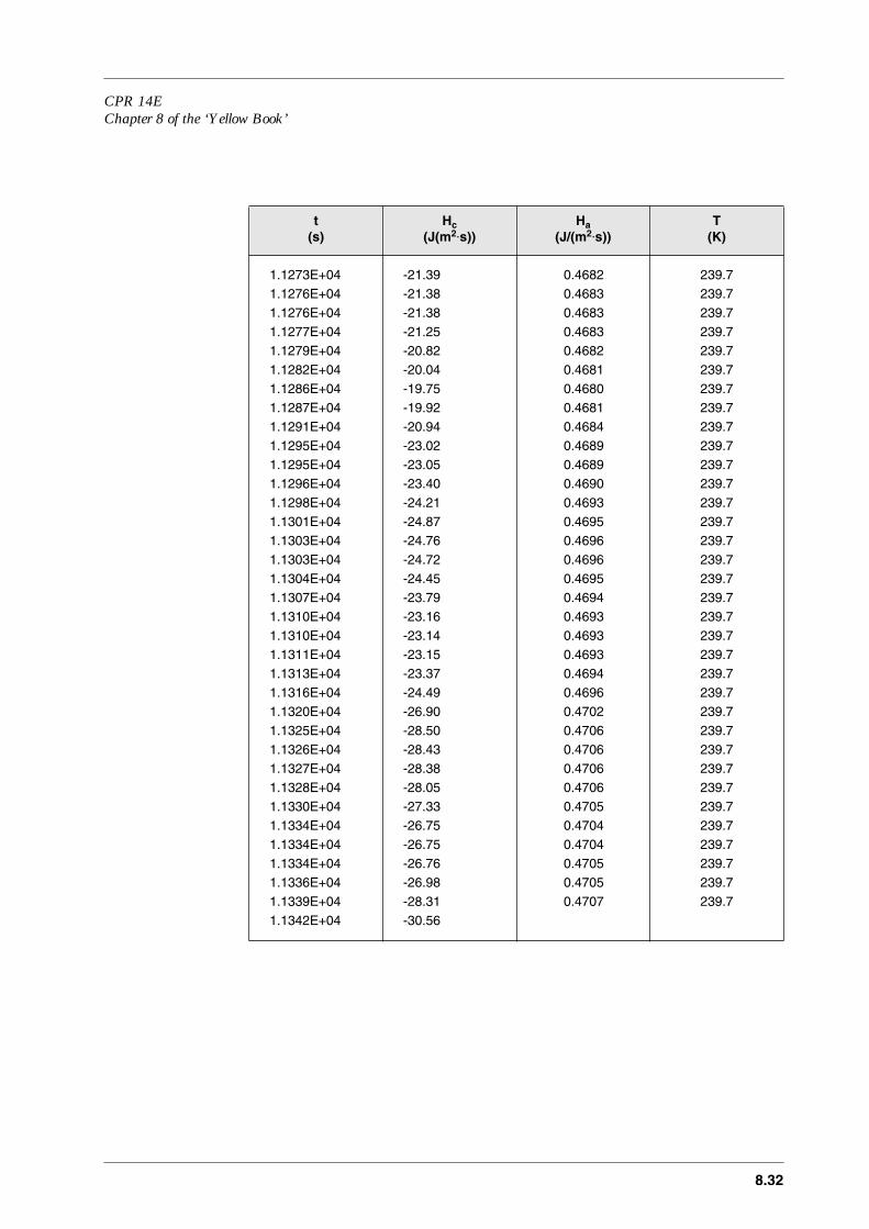
CPR 14EChapter 8 of the ‘Yellow Book’
8.32
1.1273E+04 -21.39 0.4682 239.71.1276E+04 -21.38 0.4683 239.71.1276E+04 -21.38 0.4683 239.71.1277E+04 -21.25 0.4683 239.71.1279E+04 -20.82 0.4682 239.71.1282E+04 -20.04 0.4681 239.71.1286E+04 -19.75 0.4680 239.71.1287E+04 -19.92 0.4681 239.71.1291E+04 -20.94 0.4684 239.71.1295E+04 -23.02 0.4689 239.71.1295E+04 -23.05 0.4689 239.71.1296E+04 -23.40 0.4690 239.71.1298E+04 -24.21 0.4693 239.71.1301E+04 -24.87 0.4695 239.71.1303E+04 -24.76 0.4696 239.71.1303E+04 -24.72 0.4696 239.71.1304E+04 -24.45 0.4695 239.71.1307E+04 -23.79 0.4694 239.71.1310E+04 -23.16 0.4693 239.71.1310E+04 -23.14 0.4693 239.71.1311E+04 -23.15 0.4693 239.71.1313E+04 -23.37 0.4694 239.71.1316E+04 -24.49 0.4696 239.71.1320E+04 -26.90 0.4702 239.71.1325E+04 -28.50 0.4706 239.71.1326E+04 -28.43 0.4706 239.71.1327E+04 -28.38 0.4706 239.71.1328E+04 -28.05 0.4706 239.71.1330E+04 -27.33 0.4705 239.71.1334E+04 -26.75 0.4704 239.71.1334E+04 -26.75 0.4704 239.71.1334E+04 -26.76 0.4705 239.71.1336E+04 -26.98 0.4705 239.71.1339E+04 -28.31 0.4707 239.71.1342E+04 -30.56
t(s)
Hc(J(m2⋅s))
Ha(J/(m2⋅s))
T(K)
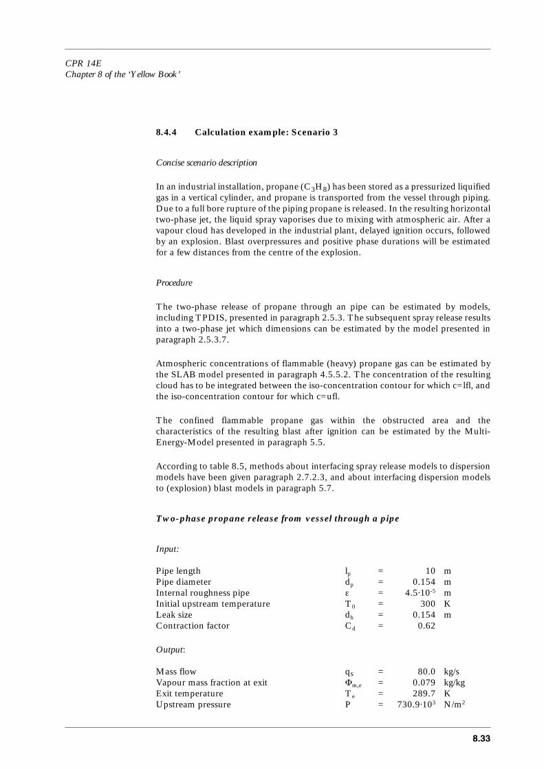
CPR 14EChapter 8 of the ‘Yellow Book’
8.33
8.4.4 Calculation example: Scenario 3
Concise scenario description
In an industrial installation, propane (C3H8) has been stored as a pressurized liquifiedgas in a vertical cylinder, and propane is transported from the vessel through piping.Due to a full bore rupture of the piping propane is released. In the resulting horizontaltwo-phase jet, the liquid spray vaporises due to mixing with atmospheric air. After avapour cloud has developed in the industrial plant, delayed ignition occurs, followedby an explosion. Blast overpressures and positive phase durations will be estimatedfor a few distances from the centre of the explosion.
Procedure
The two-phase release of propane through an pipe can be estimated by models,including TPDIS, presented in paragraph 2.5.3. The subsequent spray release resultsinto a two-phase jet which dimensions can be estimated by the model presented inparagraph 2.5.3.7.
Atmospheric concentrations of flammable (heavy) propane gas can be estimated bythe SLAB model presented in paragraph 4.5.5.2. The concentration of the resultingcloud has to be integrated between the iso-concentration contour for which c=lfl, andthe iso-concentration contour for which c=ufl.
The confined flammable propane gas within the obstructed area and thecharacteristics of the resulting blast after ignition can be estimated by the Multi-Energy-Model presented in paragraph 5.5.
According to table 8.5, methods about interfacing spray release models to dispersionmodels have been given paragraph 2.7.2.3, and about interfacing dispersion modelsto (explosion) blast models in paragraph 5.7.
Two-phase propane release from vessel through a pipe
Input:
Pipe length lp = 10 mPipe diameter dp = 0.154 mInternal roughness pipe ε = 4.5⋅10-5 mInitial upstream temperature T0 = 300 KLeak size dh = 0.154 mContraction factor Cd = 0.62
Output:
Mass flow qS = 80.0 kg/sVapour mass fraction at exit Φm,e = 0.079 kg/kgExit temperature Te = 289.7 KUpstream pressure P = 730.9⋅103 N/m2

CPR 14EChapter 8 of the ‘Yellow Book’
8.34
Note that the symbols used are conform chapter 2 'Outflow and Spray release’.
Spray release
Input:
(Average) mass flow rate qS = 80 kg/sExit temperature Te = 289.7 KExit vapour mass fraction Φm,e = 0.079 kg/kgSource exit height hs = 1 mLeak size dh = 0.154 mDischarge coefficient Cd = 0.62Ambient temperature Ta = 300 KRelative humidity RH = 70 %
Output:
Nett air-borne mass flow rate qS,nett,air = 80.00 kg/sJet diameter after rain-out bf,rainout = 0.37 mTemperature after rain-out Tf,rainout = 230.9 KVapour mass fraction after rain-out Φm,f,rainout= 0.46 kg/kg
Jet diameter after air entrainment bj = 1.47 mTemperature of air/vapour mixture Tj = 191.42 KVapour mass fraction in air/vapour mixture Φm,j = 0.46 kg/kgConcentration in air/vapour mixture cj = 0.115 m3/m3
Concentration in air/vapour mixture cj' = 0.317 kg/m3
Note that the symbols used are conform chapter 2 'Outflow and Spray release.
Heavy gas dispersion
Input:
Mass flow rate of the source qS = 80.0 kg/sDuration of release tr = 100 sMaximum diameter of expanded jet b0 = 0.37 mHeight of source h = 1.0 mVapour temperature after expansion T = 230.9 KWind velocity at 10 m height ua = 2 m/sPasquill stability class FRelative humidity RH = 70 %Ambient temperature Ta = 300 KRoughness length z0 = 1.0 m

CPR 14EChapter 8 of the ‘Yellow Book’
8.35
Output (t=10 s):
Maximum explosive mass lfl<c<ufl Qex,max = 741 kg... at time t = 40 sMaximum explosive distance xlfl,max = 164 m... at time t = 213 s
Note that the symbols used are conform chapter 4 'Vapour cloud dispersion'.
Vapour cloud explosion
Input:
Total flammable mass Qex = 741 kg
Ambient temperature Ta = 300 KStoichiometric concentration cs = 0.0706 kg/m3
Cloud volume at stoichiometric concentration Vc = 105⋅104 m3
Fraction of flammable cloud confined Vgr/Vc = 1.0 m3/m3
Strength number 10
Output:
Heat of combustion in the confined cloud E = 37.3⋅109 J
Side-on peak overpressure at 100 m Ps = 0.265⋅105 N/m2
Positive phase duration at 100 m tp = 0.053 s
Side-on peak overpressure at 200 m Ps = 0.111⋅105 N/m2
Positive phase duration at 200 m tp = 0.074 s
Side-on peak overpressure at 500 m Ps = 0.0378⋅105 N/m2
Positive phase duration at 500 m tp = 0.089 s
Note that the symbols used are conform chapter 5 'Vapour cloud explosion'.
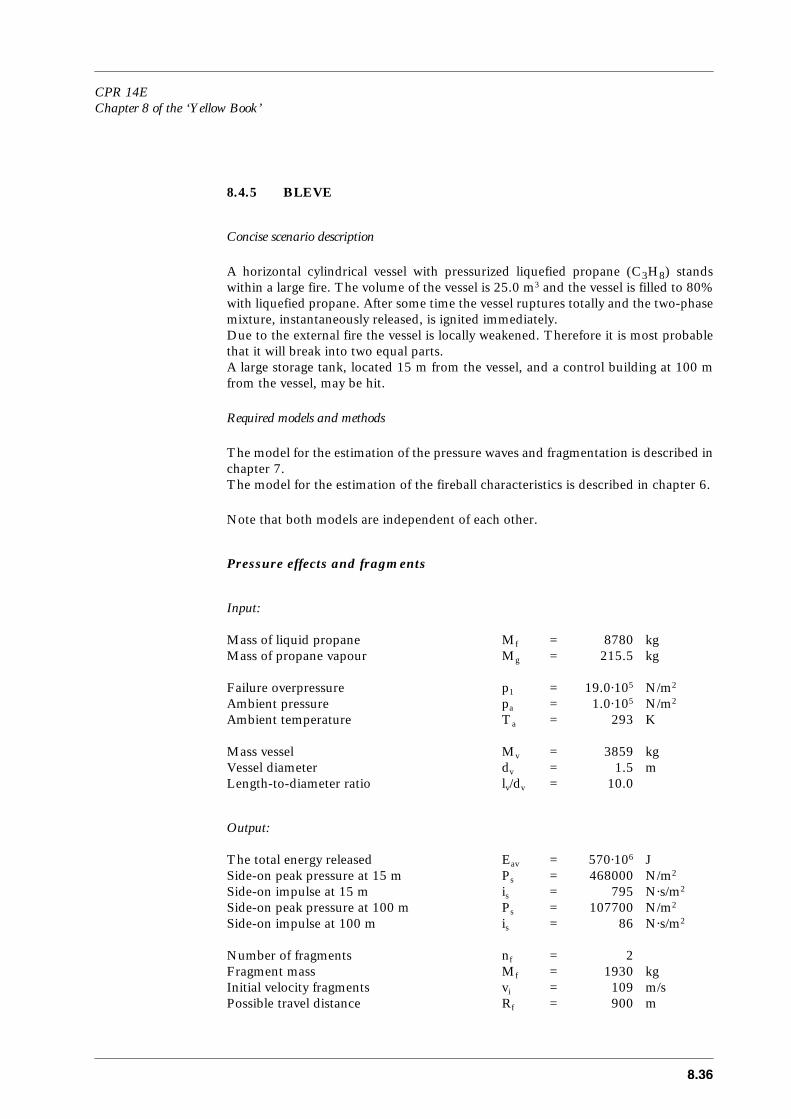
CPR 14EChapter 8 of the ‘Yellow Book’
8.36
8.4.5 BLEVE
Concise scenario description
A horizontal cylindrical vessel with pressurized liquefied propane (C3H8) standswithin a large fire. The volume of the vessel is 25.0 m3 and the vessel is filled to 80%with liquefied propane. After some time the vessel ruptures totally and the two-phasemixture, instantaneously released, is ignited immediately. Due to the external fire the vessel is locally weakened. Therefore it is most probablethat it will break into two equal parts. A large storage tank, located 15 m from the vessel, and a control building at 100 mfrom the vessel, may be hit.
Required models and methods
The model for the estimation of the pressure waves and fragmentation is described inchapter 7.The model for the estimation of the fireball characteristics is described in chapter 6.
Note that both models are independent of each other.
Pressure effects and fragments
Input:
Mass of liquid propane Mf = 8780 kgMass of propane vapour Mg = 215.5 kg
Failure overpressure p1 = 19.0⋅105 N/m2
Ambient pressure pa = 1.0⋅105 N/m2
Ambient temperature Ta = 293 K
Mass vessel Mv = 3859 kgVessel diameter dv = 1.5 mLength-to-diameter ratio lv/dv = 10.0
Output:
The total energy released Eav = 570⋅106 JSide-on peak pressure at 15 m Ps = 468000 N/m2
Side-on impulse at 15 m is = 795 N⋅s/m2
Side-on peak pressure at 100 m Ps = 107700 N/m2
Side-on impulse at 100 m is = 86 N⋅s/m2
Number of fragments nf = 2Fragment mass Mf = 1930 kgInitial velocity fragments vi = 109 m/sPossible travel distance Rf = 900 m
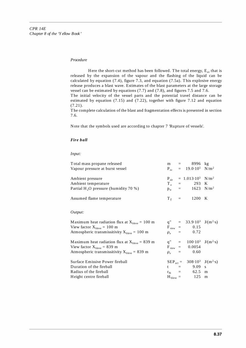
CPR 14EChapter 8 of the ‘Yellow Book’
8.37
Procedure
Here the short-cut method has been followed. The total energy, Eav that isreleased by the expansion of the vapour and the flashing of the liquid can becalculated by equation (7.4), figure 7.3, and equation (7.5a). This explosive energyrelease produces a blast wave. Estimates of the blast parameters at the large storagevessel can be estimated by equations (7.7) and (7.8), and figures 7.5 and 7.6.The initial velocity of the vessel parts and the potential travel distance can beestimated by equation (7.15) and (7.22), together with figure 7.12 and equation(7.21).The complete calculation of the blast and fragmentation effects is presented in section7.6.
Note that the symbols used are according to chapter 7 'Rupture of vessels'.
Fire ball
Input:
Total mass propane released m = 8996 kgVapour pressure at burst vessel Psv = 19.0⋅105 N/m2
Ambient pressure Pair = 1.013⋅105 N/m2
Ambient temperature Ta = 293 KPartial H2O pressure (humidity 70 %) pw = 1623 N/m2
Assumed flame temperature Tf = 1200 K
Output:
Maximum heat radiation flux at Xbleve = 100 m q" = 33.9⋅103 J/(m2⋅s)View factor Xbleve = 100 m Fview = 0.15Atmospheric transmissitivity Xbleve = 100 m ρa = 0.72
Maximum heat radiation flux at Xbleve = 839 m q" = 100⋅103 J/(m2⋅s)View factor Xbleve = 839 m Fview = 0.0054Atmospheric transmissitivity Xbleve = 839 m ρa = 0.60
Surface Emissive Power fireball SEPact = 308⋅103 J/(m2⋅s)Duration of the fireball t = 9.09 sRadius of the fireball rfb = 62.5 mHeight centre fireball Hbleve = 125 m

CPR 14EChapter 8 of the ‘Yellow Book’
8.38
Procedure
The radius, duration and lift-off height of the fire ball can be calculated by equations(6.90), (6.91) and (6.22), respectively.The straight distance between the centre of the fire ball to the receptor can becalculated by equation (6.92) based on the horizontal distance to the vessel and thelift-off height of the fire ball.The view factor, depending on the radius of the fire ball and the distance to the centreof the fireball, can be calculated by equation (6.93). The surface emissive power ofthe fire ball can be estimated by equations (6.21) and (6.95). The heat flux thereceptor is receiving, depends on the surface emissive power, atmospherictransmissitivity and the view factor, and can be estimated by equation (6.4).The complete calculation of heat flux due to a fire ball, caused by an ignition of aBLEVE, is presented in section 6.6.5.
Note that the symbols used are according to chapter 6 'Heat fluxes from fires'.
CPR 14EChapter 8 of the ‘Yellow Book’
8.39
8.5 Discussion and conclusions
Interfacing of models deals with the transfer of data from a previous modelto a subsequent model in the chain representing a scenario.
The chain of models necessary to quantify the physical effects is depending on theavailability of existing (computerised) models. Models vary in degree of complexityand detail, and have a common tendency to describe highly idealised laboratorysituations in which one single phenomenon is under study. Consequently, thedetailed predictions of the prior model have to be simplified in order to serve as inputfor the next model. This simplification always results in a loss of information and thusfinal predictions deteriorate to some extent.
In theory, integral models should be able to preserve all information about priorphysical phenomena, taking into account variations in time and magnitude.However, improved predictions are not necessary for all types of (safety-) studies.The description of such integral models is much more complicated because of the factthat more details have to be taken into account and a special dedicated numericalprocedure must be applied. The large numerical integral procedure this approachwould require, would further enlarge the required computational capacity.For the present, the maximum degree of model complexity has been reached bymodels such as GASP in chapter 3 ‘Pool Evaporation’, that are still reasonablymanageable in safety and risk assessment studies.
Several types of physical effects are possible for a given set of accident conditions.Furthermore, hazardous materials may follow more than one route leading toparticular consequences. Thus, more than one scenario may be required to fully access all possible physicaleffects causing damage. These scenarios differ from each other by a different kind ofspill of hazardous material under particular process and meteorological conditions.
In case the released hazardous material will react and form toxic reaction products,the list of scenarios can easily be extended to follow-up scenarios. The best way toavoid endless repetitions of very similar scenarios is to consider the reaction productsof the primary hazardous material released, and look for the most fitting scenario.
Always the possibility of so-called domino-effects is apparent, i.e. triggering ofsecondary events by a primary event such that the result is an increase inconsequences or area of an effect zone. These domino effects are generally onlyconsidered if they result in a significant escalation of the original incident.

CPR 14EChapter 8 of the ‘Yellow Book’
8.40
8.6 References
AIChE (1989),Chemical Process Quantitative Risk Analysis – guidelines for –, Center for Chemical Process Safety of the American Institute of Chemical Engineers,1989.
Bosch (1992),C.J.H.van den Bosch, H. Bekkering,System description IRIS: Effect Module, TNO-report 92-054, for the NetherlandsMinistry for Home Affairs, 11-2-92.
Potts (1981),Hazard Assessment Computer System -Users’ operation manual vol.1-,R.G. Potts, A.D. LITTLE for US Coast Guard, 30-09-81.

annex-1
AnnexPhysical properties of chemicalsC.J.H. van den Bosch

Annex-2
List of symbols Annex
clfl Concentration at lower flammability limit kg/m3
cufl Concentration at upper flammability limit kg/m3
cS Maximum solubility in water kg/m3
Cp,g Specific heat gas/vapour J/(mol⋅K)Cp,L Specific heat liquid J/(kg⋅K)CX,... Coefficient ‘X’ of temperature relation -LFL Lower flammability limit vol%UFL Upper flammability limit vol%P˚ Vapour pressure N/m2
Pc Critical pressure N/m2
Tb Boiling point KTc Critical temperature KTfl Flash point KTm Melting point K
Greek symbols
γ Poisson ratio Cp,g/Cv,g -∆Hc Heat of combustion J/kgLv Heat of vaporisation J/kgηg Dynamic viscosity gas/vapour N⋅s/m2
ηL Dynamic viscosity liquid N⋅s/m2
µ Molecular weight kg/molρg Gas/vapour density kg/m3
ρL Liquid density kg/m3
σ Surface tension N/m

CPR 14EAnnex of the ‘Yellow Book’
Annex-3
Table of contents of Annex
List of symbols Annex..............................................................annex-2
A.1 Introduction .............................................................................annex-5
A.2 References ................................................................................annex-9
A.3 Data physical properties..........................................................annex-11

Annex-4
A.1 Introduction
For several chemicals physical properties are given as physical constants oras coefficients of relations expressing properties’ temperature dependency.Data has been collected from various sources. Most individual sources do not provideall physical properties required. All sources referred to have been used to compile adata set of physical constants and coefficients, as complete as possible.
Physical constants are given for each chemical.The chemical specific coefficients of the temperature relations are given for eachchemical. Using these equations the physical properties can be calculated for anytemperature, within the valid range.
Values for the temperature-dependent physical properties are given forT = 288.15 K (15 ˚C).
Physical properties given as physical constant:
Molecular weight µMelting point Tm
Boiling point Tb
Critical temperature Tc
Critical pressure Pc
Flash point Tfl
Heat of combustion ∆Hc
Lower flammability limit LFLUpper flammability limit UFLSolubility in water cS
Physical properties given as a function of absolute temperature:
Specific heat gas/vapour Cp,g
Poisson ratio Cp,g/Cv,g γGas/vapour density ρg
Gas/vapour viscosity ηg
Vapour pressure P˚Heat of vaporisation Lv
Specific heat liquid Cp,L
Liquid density ρL
Liquid viscosity ηL
Surface tension σ
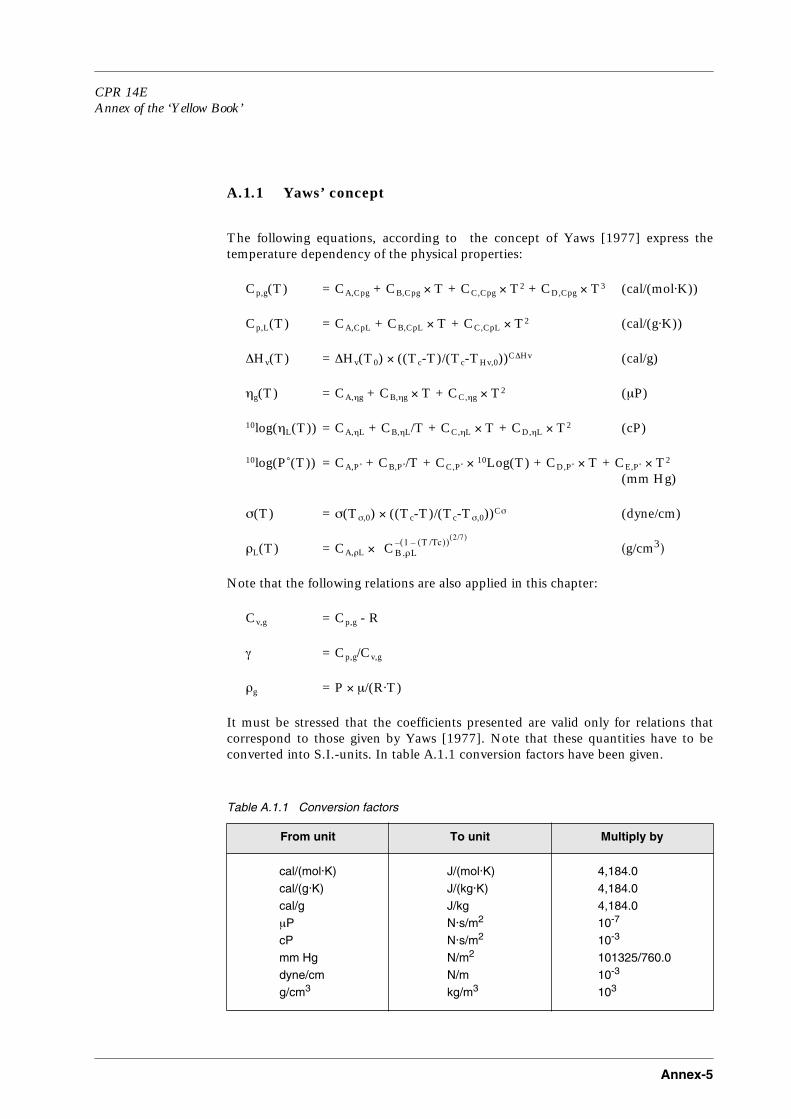
CPR 14EAnnex of the ‘Yellow Book’
Annex-5
A.1.1 Yaws’ concept
The following equations, according to the concept of Yaws [1977] express thetemperature dependency of the physical properties:
Cp,g(T) = CA,Cpg + CB,Cpg × T + CC,Cpg × T2 + CD,Cpg × T3 (cal/(mol⋅K))
Cp,L(T) = CA,CpL + CB,CpL × T + CC,CpL × T2 (cal/(g⋅K))
∆Hv(T) = ∆Hv(T0) × ((Tc-T)/(Tc-THv,0))C∆Hv (cal/g)
ηg(T) = CA,ηg + CB,ηg × T + CC,ηg × T2 (µP)
10log(ηL(T)) = CA,ηL + CB,ηL/T + CC,ηL × T + CD,ηL × T2 (cP)
10log(P˚(T)) = CA,P˚ + CB,P˚/T + CC,P˚ × 10Log(T) + CD,P˚ × T + CE,P˚ × T2
(mm Hg)
σ(T) = σ(Tσ,0) × ((Tc-T)/(Tc-Tσ,0))Cσ (dyne/cm)
ρL(T) = CA,ρL × (g/cm3)
Note that the following relations are also applied in this chapter:
Cv,g = Cp,g - R
γ = Cp,g/Cv,g
ρg = P × µ/(R⋅T)
It must be stressed that the coefficients presented are valid only for relations thatcorrespond to those given by Yaws [1977]. Note that these quantities have to beconverted into S.I.-units. In table A.1.1 conversion factors have been given.
Table A.1.1 Conversion factors
From unit To unit Multiply by
cal/(mol⋅K) J/(mol⋅K) 4,184.0cal/(g⋅K) J/(kg⋅K) 4,184.0cal/g J/kg 4,184.0µP N⋅s/m2 10-7
cP N⋅s/m2 10-3
mm Hg N/m2 101325/760.0dyne/cm N/m 10-3
g/cm3 kg/m3 103
CB ,ρL1 T/Tc( )–( )
2/7( )–
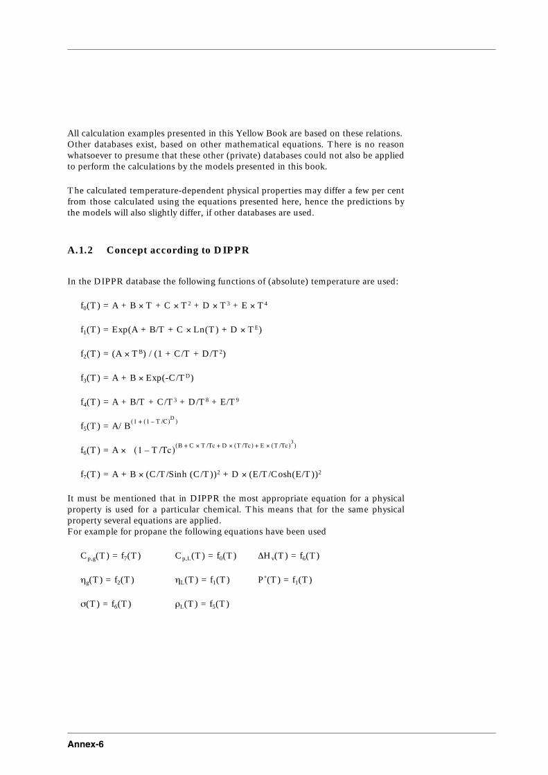
Annex-6
All calculation examples presented in this Yellow Book are based on these relations.Other databases exist, based on other mathematical equations. There is no reasonwhatsoever to presume that these other (private) databases could not also be appliedto perform the calculations by the models presented in this book.
The calculated temperature-dependent physical properties may differ a few per centfrom those calculated using the equations presented here, hence the predictions bythe models will also slightly differ, if other databases are used.
A.1.2 Concept according to DIPPR
In the DIPPR database the following functions of (absolute) temperature are used:
f0(T) = A + B × T + C × T2 + D × T3 + E × T4
f1(T) = Exp(A + B/T + C × Ln(T) + D × TE)
f2(T) = (A × TB) / (1 + C/T + D/T2)
f3(T) = A + B × Exp(-C/TD)
f4(T) = A + B/T + C/T3 + D/T8 + E/T9
f5(T) = A/
f6(T) = A ×
f7(T) = A + B × (C/T/Sinh (C/T))2 + D × (E/T/Cosh(E/T))2
It must be mentioned that in DIPPR the most appropriate equation for a physicalproperty is used for a particular chemical. This means that for the same physicalproperty several equations are applied.For example for propane the following equations have been used
Cp,g(T) = f7(T) Cp,L(T) = f0(T) ∆Hv(T) = f6(T)
ηg(T) = f2(T) ηL(T) = f1(T) P˚(T) = f1(T)
σ(T) = f6(T) ρL(T) = f5(T)
B1 1 T/C–( )
D+( )
1 T/Tc–( )B C T/Tc D T/Tc( ) E T/Tc( )
3×+×+×+( )

CPR 14EAnnex of the ‘Yellow Book’
Annex-7
A.2 References
Chem (1995),Chemiekaarten - Gegevens voor het veilig werken met chemicaliën, NIA/VNCI/Samsom H.D. Tjeenk Willink, 10e editie, Alphen a/d Rijn 1994-95.
CRC (1995),Handbook of Chemistry and Physics, CRC Press, 75th ed., 1995
DIPPR (1990),Th. B. Selover, Use of DIPPr data in reactive chemical hazard assessment, Plant/Operations Progress,9(4),207-212,October 1990.
LandoltLandolt-Börnstein, Zahlenwerte und Funktionen, Springer-Verlag.
Yaws (1977),C.L. Yaws, Physical Properties, McGraw-Hill, New York, 1977.
Annex-8
A.3 Data physical properties
Physical properties are listed for the following chemicals:
1. ACROLEIN ................................................................................annex-9
2. ACRYLONITRILE .....................................................................annex-11
3. AIR .............................................................................................annex-13
4. AMMONIA.................................................................................annex-15
5. BUTANE (n-) .............................................................................annex-17
6. CARBON MONOXIDE..............................................................annex-19
7. CARBONDISULFIDE................................................................annex-21
8. CHLORINE................................................................................annex-23
9. ETHENE ....................................................................................annex-25
10. GASOLINE ................................................................................annex-27
11. HYDROGEN.............................................................................annex-29
12. HYDROGEN CHLORIDE .........................................................annex-31
13. HYDROGEN CYANIDE............................................................annex-33
14. HYDROGEN FLUORIDE..........................................................annex-35
15. HYDROGEN SULFIDE.............................................................annex-37
16. METHANE ................................................................................annex-39
17. METHANOL..............................................................................annex-41
18. METHYL MERCAPTAN...........................................................annex-43
19. NITROGEN DIOXIDE ..............................................................annex-45
20. PROPANE ..................................................................................annex-47
21. PROPENE ..................................................................................annex-49
22. SULPHUR DIOXIDE.................................................................annex-51
23. TOLUENE .................................................................................annex-53
24. WATER ......................................................................................annex-55

CPR 14EAnnex of the ‘Yellow Book’
Annex-9
1. ACROLEIN
Material_Name = ACROLEINMolecular formula = CH2CHCHOUN number = 1092Molecular weight = 56.060000 kg/kmolCritical temperature = 506.000000 K (232.85 °C)Melting point = 185.450000 K (-87.70 °C)Triplepoint temperature = 185.450000 K (-87.70 °C)Normal boiling point = 325.840000 K (52.69 °C)Standard net heat of combustion = 2.771000E+0007 J/kg ( 1.553423E+0009 J/kmol)Flash point = 247.150000 K (-26.00 °C)Lower flammability limit = 2.800000 vol% in airUpper flammability limit = 100.000000 vol% in airSolubility in water = 206.000000 kg/m3
Temperature dependent data (calculated at 288.15 K (15.00 °C)Liquid density = 8.440330E+0002 kg/m3 (844.03 kg/m3 )Vapor pressure = 2.399542E+0004 N/m2 (0.24 Bar )Heat of vaporization = 5.478413E+0005 J/kg (547841.26 J/kg )Liquid heatcapacity = 2.151910E+0003 J/kg*K (2151.91 J/kg*K)Gas heatcapacity (ideal gas) = 1.130799E+0003 J/kg*K (1130.80 J/kg*K)Liquid viscosity = 3.649874E-0004 Pa*s Vapor viscosity = 8.227617E-0006 Pa*s Surface tension = 2.456317E-0002 N/m Poisson ratio = 1.151
Functions (calculated at 288.15 K (15.00 °C) and 1.000000E+05 N/m2 (1.000 Bar)Gas density (ideal gas law) : 2.340 kg/m3Mass of 1 m3 gas/vapour : 2.340 kgVolume of 1 kg gas/vapour : 0.427 m3Mass of 1 m3 liquid : 844.033 kgVolume of 1000 kg liquid : 1.185 m3
Probit constants (Toxicity)A = 5.621200 SI units(Kg*s/m3)B = 1.000000 SI units(Kg*s/m3)N = 1.000000 SI units(Kg*s/m3)
A = -3.251597 (ppm*min)B = 1.000000 (ppm*min)N = 1.000000 (ppm*min)
A = -4.099966 (mg*min/m3)B = 1.000000 (mg*min/m3)N = 1.000000 (mg*min/m3)
Temperature dependent data (Parameters):
Liquid densityFormula Nr. 1 rho = A * B^-((1-T/C)^2/7) (where C=Tc) [g/cm3] [g/cm3]Minimum temperature = 185.450000 [K]Maximum temperature = 506.000000 [K]Parameter 1 = 3.228800E-0001Parameter 2 = 2.944900E-0001Parameter 3 = 5.060000E+0002Parameter 4 = 0.000000E+0000Parameter 5 = 0.000000E+0000

Annex-10
Vapor pressureFormula Nr. 2 Log(P) = A + B/T + C*Log(T) + D*T + E*T^2 [mm Hg] [mm Hg]Minimum temperature = 185.450000 [K]Maximum temperature = 506.000000 [K]Parameter 1 = 3.900860E+0001Parameter 2 = -2.746400E+0003Parameter 3 = -1.117600E+0001Parameter 4 = -1.054000E-0003Parameter 5 = 6.868000E-0006
Heat of vaporizationFormula Nr. 3 Hv = A * ((C-T)/(C-B)^D (A=Hv1, B=T1, C=Tc) [cal/g] [cal/g]Minimum temperature = 185.450000 [K]Maximum temperature = 506.000000 [K]Parameter 1 = 1.195000E+0002Parameter 2 = 3.457000E+0002Parameter 3 = 5.060000E+0002Parameter 4 = 2.964000E-0001Parameter 5 = 0.000000E+0000
Liquid heatcapacityFormula Nr. 4 Cpl = A + B*T + C*T^2 + D*T^3 [cal/g/K] [cal/g/K]Minimum temperature = 275.000000 [K]Maximum temperature = 350.000000 [K]Parameter 1 = 3.669900E-0001Parameter 2 = 4.970900E-0004Parameter 3 = 6.687800E-0008Parameter 4 = -7.132000E-0011Parameter 5 = 0.000000E+0000
IG heatcapacityFormula Nr. 5 Cp = A + B*T + C*T^2 + D*T^3 [cal/mol] [cal/mol]Minimum temperature = 298.150000 [K]Maximum temperature = 1000.100000 [K]Parameter 1 = 4.864400E+0000Parameter 2 = 2.794800E-0002Parameter 3 = 2.931600E-0005Parameter 4 = -2.487000E-0008Parameter 5 = 0.000000E+0000
Liquid viscosityFormula Nr. 6 Log(Visc) = Ea + Eb/T + Ec*Log (T) + Ed*T + Ee*T*T (where Ec=0!) [centiPoise][centiPoise]Minimum temperature = 222.890000 [K]Maximum temperature = 353.220000 [K]Parameter 1 = -1.791500E+0000Parameter 2 = 3.689500E+0002Parameter 3 = 0.000000E+0000Parameter 4 = 3.078400E-0004Parameter 5 = -1.847000E-0007
Vapor viscosityFormula Nr. 7 Visc = A + B*T + C*T^2 [microPoise] [microPoise]Minimum temperature = 325.840000 [K]Maximum temperature = 995.840000 [K]Parameter 1 = -1.718200E+0001Parameter 2 = 3.226100E-0001Parameter 3 = -5.332000E-0005Parameter 4 = 0.000000E+0000Parameter 5 = 0.000000E+0000
Surface TensionFormula Nr. 8 Sigma = A * ((C-T)/(C-B))^D (A=Sigma1, B=T1, C=Tc) [dynes/cm] [dynes/cm]Minimum temperature = 185.450000 [K]Maximum temperature = 506.000000 [K]Parameter 1 = 1.658000E+0001Parameter 2 = 3.457000E+0002Parameter 3 = 5.060000E+0002Parameter 4 = 1.281300E+0000Parameter 5 = 0.000000E+0000

CPR 14EAnnex of the ‘Yellow Book’
Annex-11
2. ACRYLONITRILE
Material_Name = ACRYLONITRILEMolecular formula = CH2CHCNUN number = 1093Molecular weight = 53.060000 kg/kmolCritical temperature = 535.000000 K (261.85 °C)Melting point = 189.630000 K (-83.52 °C)Triplepoint temperature = 189.630000 K (-83.52 °C)Normal boiling point = 350.500000 K (77.35 °C)Standard net heat of combustion = 3.184800E+0007 J/kg ( 1.689855E+0009 J/kmol)Flash point = 273.150000 K (-0.00 °C)Lower flammability limit = 2.420000 vol% in airUpper flammability limit = 100.000000 vol% in airSolubility in water = 73.000000 kg/m3
Temperature dependent data (calculated at 288.15 K (15.00 °C)Liquid density = 8.124973E+0002 kg/m3 (812.50 kg/m3 )Vapor pressure = 9.106335E+0003 N/m2 (0.09 Bar )Heat of vaporization = 6.336796E+0005 J/kg (633679.62 J/kg )Liquid heatcapacity = 2.029729E+0003 J/kg*K (2029.73 J/kg*K)Gas heatcapacity (ideal gas) = 1.187232E+0003 J/kg*K (1187.23 J/kg*K)Liquid viscosity = 3.683722E-0004 Pa*s Vapor viscosity = 6.674399E-0006 Pa*s Surface tension = 2.790906E-0002 N/m Poisson ratio = 1.152
Functions (calculated at 288.15 K (15.00 °C) and 1.000000E+05 N/m2 (1.000 Bar)Gas density (ideal gas law) : 2.215 kg/m3Mass of 1 m3 gas/vapour : 2.215 kgVolume of 1 kg gas/vapour : 0.452 m3Mass of 1 m3 liquid : 812.497 kgVolume of 1000 kg liquid : 1.231 m3
Probit constants (Toxicity)A = 5.265800 SI units(Kg*s/m3)B = 1.000000 SI units(Kg*s/m3)N = 1.300000 SI units(Kg*s/m3)
A = -7.568639 (ppm*min)B = 1.000000 (ppm*min)N = 1.300000 (ppm*min)
A = -8.600019 (mg*min/m3)B = 1.000000 (mg*min/m3)N = 1.300000 (mg*min/m3)
Temperature dependent data (Parameters):
Liquid densityFormula Nr. 1 rho = A * B^-((1-T/C)^2/7) (where C=Tc) [g/cm3] [g/cm3]Minimum temperature = 189.630000 [K]Maximum temperature = 535.000000 [K]Parameter 1 = 2.470400E-0001Parameter 2 = 2.265000E-0001Parameter 3 = 5.350000E+0002Parameter 4 = 0.000000E+0000Parameter 5 = 0.000000E+0000
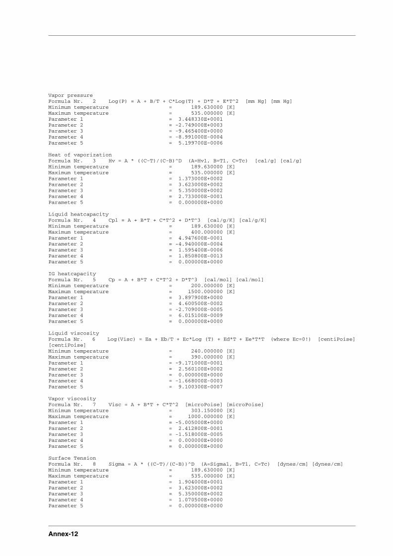
Annex-12
Vapor pressureFormula Nr. 2 Log(P) = A + B/T + C*Log(T) + D*T + E*T^2 [mm Hg] [mm Hg]Minimum temperature = 189.630000 [K]Maximum temperature = 535.000000 [K]Parameter 1 = 3.448330E+0001Parameter 2 = -2.749000E+0003Parameter 3 = -9.465400E+0000Parameter 4 = -8.991000E-0004Parameter 5 = 5.199700E-0006
Heat of vaporizationFormula Nr. 3 Hv = A * ((C-T)/(C-B)^D (A=Hv1, B=T1, C=Tc) [cal/g] [cal/g]Minimum temperature = 189.630000 [K]Maximum temperature = 535.000000 [K]Parameter 1 = 1.373000E+0002Parameter 2 = 3.623000E+0002Parameter 3 = 5.350000E+0002Parameter 4 = 2.733000E-0001Parameter 5 = 0.000000E+0000
Liquid heatcapacityFormula Nr. 4 Cpl = A + B*T + C*T^2 + D*T^3 [cal/g/K] [cal/g/K]Minimum temperature = 189.630000 [K]Maximum temperature = 400.000000 [K]Parameter 1 = 4.947600E-0001Parameter 2 = -4.940000E-0004Parameter 3 = 1.595400E-0006Parameter 4 = 1.850800E-0013Parameter 5 = 0.000000E+0000
IG heatcapacityFormula Nr. 5 Cp = A + B*T + C*T^2 + D*T^3 [cal/mol] [cal/mol]Minimum temperature = 200.000000 [K]Maximum temperature = 1500.000000 [K]Parameter 1 = 3.897900E+0000Parameter 2 = 4.600500E-0002Parameter 3 = -2.709000E-0005Parameter 4 = 6.015100E-0009Parameter 5 = 0.000000E+0000
Liquid viscosityFormula Nr. 6 Log(Visc) = Ea + Eb/T + Ec*Log (T) + Ed*T + Ee*T*T (where Ec=0!) [centiPoise][centiPoise]Minimum temperature = 240.000000 [K]Maximum temperature = 390.000000 [K]Parameter 1 = -9.171000E-0001Parameter 2 = 2.560100E+0002Parameter 3 = 0.000000E+0000Parameter 4 = -1.668000E-0003Parameter 5 = 9.100300E-0007
Vapor viscosityFormula Nr. 7 Visc = A + B*T + C*T^2 [microPoise] [microPoise]Minimum temperature = 303.150000 [K]Maximum temperature = 1000.000000 [K]Parameter 1 = -5.005000E+0000Parameter 2 = 2.412800E-0001Parameter 3 = -1.518000E-0005Parameter 4 = 0.000000E+0000Parameter 5 = 0.000000E+0000
Surface TensionFormula Nr. 8 Sigma = A * ((C-T)/(C-B))^D (A=Sigma1, B=T1, C=Tc) [dynes/cm] [dynes/cm]Minimum temperature = 189.630000 [K]Maximum temperature = 535.000000 [K]Parameter 1 = 1.904000E+0001Parameter 2 = 3.623000E+0002Parameter 3 = 5.350000E+0002Parameter 4 = 1.070500E+0000Parameter 5 = 0.000000E+0000
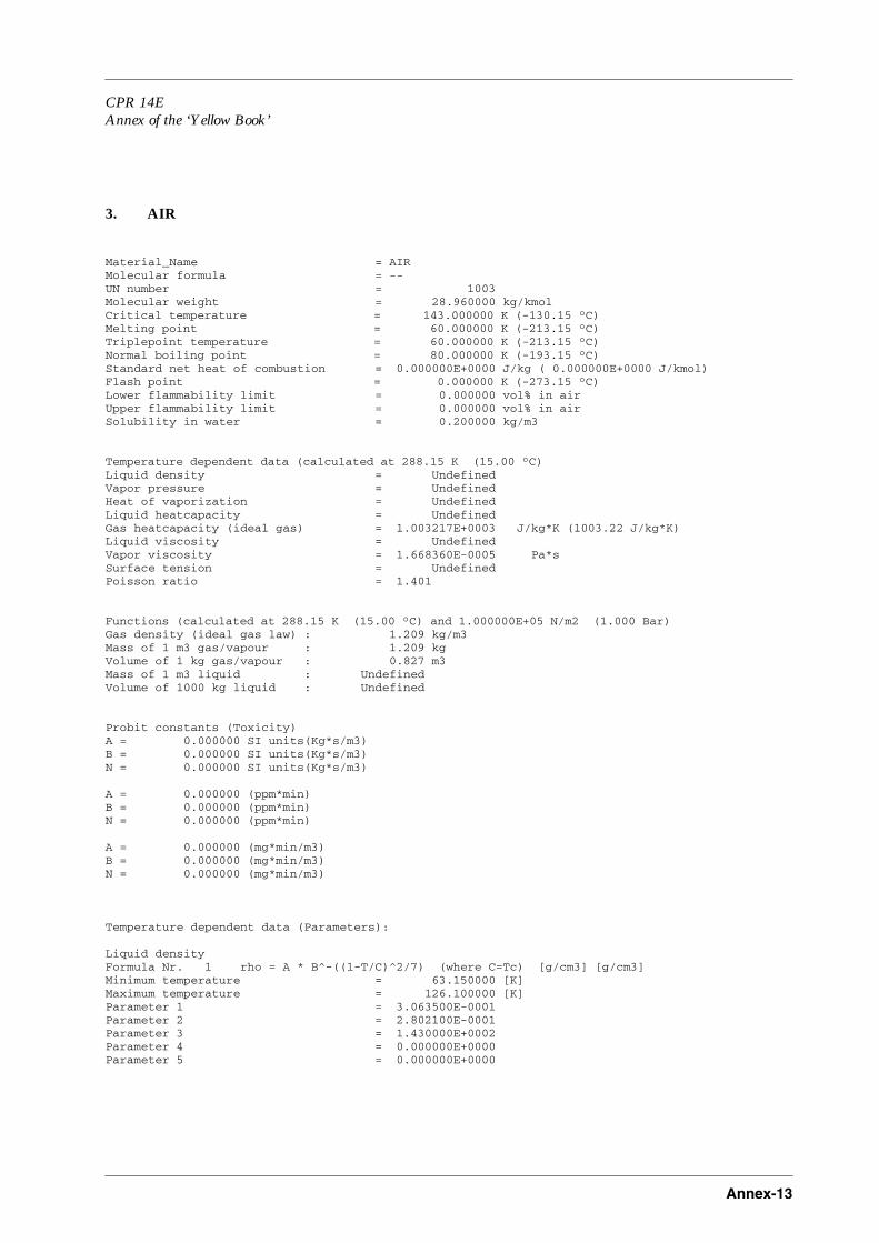
CPR 14EAnnex of the ‘Yellow Book’
Annex-13
3. AIR
Material_Name = AIRMolecular formula = --UN number = 1003Molecular weight = 28.960000 kg/kmolCritical temperature = 143.000000 K (-130.15 °C)Melting point = 60.000000 K (-213.15 °C)Triplepoint temperature = 60.000000 K (-213.15 °C)Normal boiling point = 80.000000 K (-193.15 °C)Standard net heat of combustion = 0.000000E+0000 J/kg ( 0.000000E+0000 J/kmol)Flash point = 0.000000 K (-273.15 °C)Lower flammability limit = 0.000000 vol% in airUpper flammability limit = 0.000000 vol% in airSolubility in water = 0.200000 kg/m3
Temperature dependent data (calculated at 288.15 K (15.00 °C)Liquid density = UndefinedVapor pressure = UndefinedHeat of vaporization = UndefinedLiquid heatcapacity = UndefinedGas heatcapacity (ideal gas) = 1.003217E+0003 J/kg*K (1003.22 J/kg*K)Liquid viscosity = UndefinedVapor viscosity = 1.668360E-0005 Pa*s Surface tension = UndefinedPoisson ratio = 1.401
Functions (calculated at 288.15 K (15.00 °C) and 1.000000E+05 N/m2 (1.000 Bar)Gas density (ideal gas law) : 1.209 kg/m3Mass of 1 m3 gas/vapour : 1.209 kgVolume of 1 kg gas/vapour : 0.827 m3Mass of 1 m3 liquid : UndefinedVolume of 1000 kg liquid : Undefined
Probit constants (Toxicity)A = 0.000000 SI units(Kg*s/m3)B = 0.000000 SI units(Kg*s/m3)N = 0.000000 SI units(Kg*s/m3)
A = 0.000000 (ppm*min)B = 0.000000 (ppm*min)N = 0.000000 (ppm*min)
A = 0.000000 (mg*min/m3)B = 0.000000 (mg*min/m3)N = 0.000000 (mg*min/m3)
Temperature dependent data (Parameters):
Liquid densityFormula Nr. 1 rho = A * B^-((1-T/C)^2/7) (where C=Tc) [g/cm3] [g/cm3]Minimum temperature = 63.150000 [K]Maximum temperature = 126.100000 [K]Parameter 1 = 3.063500E-0001Parameter 2 = 2.802100E-0001Parameter 3 = 1.430000E+0002Parameter 4 = 0.000000E+0000Parameter 5 = 0.000000E+0000

Annex-14
Vapor pressureFormula Nr. 2 Log(P) = A + B/T + C*Log(T) + D*T + E*T^2 [mm Hg] [mm Hg]Minimum temperature = 63.150000 [K]Maximum temperature = 126.100000 [K]Parameter 1 = 2.208250E+0001Parameter 2 = -4.636600E+0002Parameter 3 = -7.642500E+0000Parameter 4 = 1.512500E-0002Parameter 5 = 9.202400E-0006
Heat of vaporizationFormula Nr. 3 Hv = A * ((C-T)/(C-B)^D (A=Hv1, B=T1, C=Tc) [cal/g] [cal/g]Minimum temperature = 63.150000 [K]Maximum temperature = 126.100000 [K]Parameter 1 = 4.082000E+0001Parameter 2 = 9.463000E+0001Parameter 3 = 1.430000E+0002Parameter 4 = 3.875700E-0001Parameter 5 = 0.000000E+0000
Liquid heatcapacityFormula Nr. 4 Cpl = A + B*T + C*T^2 + D*T^3 [cal/g/K] [cal/g/K]Minimum temperature = 64.000000 [K]Maximum temperature = 120.000000 [K]Parameter 1 = 9.990900E-0001Parameter 2 = -1.390000E-0002Parameter 3 = 9.090500E-0005Parameter 4 = 2.520200E-0008Parameter 5 = 0.000000E+0000
IG heatcapacityFormula Nr. 5 Cp = A + B*T + C*T^2 + D*T^3 [cal/mol] [cal/mol]Minimum temperature = 250.000000 [K]Maximum temperature = 1500.000000 [K]Parameter 1 = 7.064000E+0000Parameter 2 = -1.256000E-0003Parameter 3 = 3.227700E-0006Parameter 4 = -1.234000E-0009Parameter 5 = 0.000000E+0000
Liquid viscosityFormula Nr. 6 Log(Visc) = Ea + Eb/T + Ec*Log (T) + Ed*T + Ee*T*T (where Ec=0!) [centiPoise][centiPoise]Minimum temperature = 63.150000 [K]Maximum temperature = 125.000000 [K]Parameter 1 = -7.685000E-0001Parameter 2 = 4.193500E+0001Parameter 3 = 0.000000E+0000Parameter 4 = -7.046000E-0003Parameter 5 = -1.886000E-0006
Vapor viscosityFormula Nr. 7 Visc = A + B*T + C*T^2 [microPoise] [microPoise]Minimum temperature = 80.000000 [K]Maximum temperature = 1500.000000 [K]Parameter 1 = 2.202900E+0001Parameter 2 = 5.434000E-0001Parameter 3 = -1.418000E-0004Parameter 4 = 0.000000E+0000Parameter 5 = 0.000000E+0000
Surface TensionFormula Nr. 8 Sigma = A * ((C-T)/(C-B))^D (A=Sigma1, B=T1, C=Tc) [dynes/cm] [dynes/cm]Minimum temperature = 63.150000 [K]Maximum temperature = 126.100000 [K]Parameter 1 = 5.143000E+0000Parameter 2 = 9.463000E+0001Parameter 3 = 1.430000E+0002Parameter 4 = 1.245700E+0000Parameter 5 = 0.000000E+0000
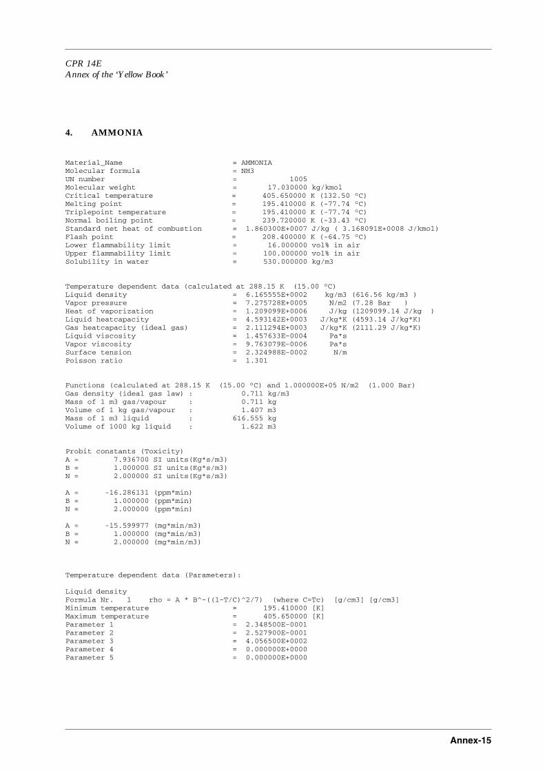
CPR 14EAnnex of the ‘Yellow Book’
Annex-15
4. AMMONIA
Material_Name = AMMONIAMolecular formula = NH3UN number = 1005Molecular weight = 17.030000 kg/kmolCritical temperature = 405.650000 K (132.50 °C)Melting point = 195.410000 K (-77.74 °C)Triplepoint temperature = 195.410000 K (-77.74 °C)Normal boiling point = 239.720000 K (-33.43 °C)Standard net heat of combustion = 1.860300E+0007 J/kg ( 3.168091E+0008 J/kmol)Flash point = 208.400000 K (-64.75 °C)Lower flammability limit = 16.000000 vol% in airUpper flammability limit = 100.000000 vol% in airSolubility in water = 530.000000 kg/m3
Temperature dependent data (calculated at 288.15 K (15.00 °C)Liquid density = 6.165555E+0002 kg/m3 (616.56 kg/m3 )Vapor pressure = 7.275728E+0005 N/m2 (7.28 Bar )Heat of vaporization = 1.209099E+0006 J/kg (1209099.14 J/kg )Liquid heatcapacity = 4.593142E+0003 J/kg*K (4593.14 J/kg*K)Gas heatcapacity (ideal gas) = 2.111294E+0003 J/kg*K (2111.29 J/kg*K)Liquid viscosity = 1.457633E-0004 Pa*s Vapor viscosity = 9.763079E-0006 Pa*s Surface tension = 2.324988E-0002 N/m Poisson ratio = 1.301
Functions (calculated at 288.15 K (15.00 °C) and 1.000000E+05 N/m2 (1.000 Bar)Gas density (ideal gas law) : 0.711 kg/m3Mass of 1 m3 gas/vapour : 0.711 kgVolume of 1 kg gas/vapour : 1.407 m3Mass of 1 m3 liquid : 616.555 kgVolume of 1000 kg liquid : 1.622 m3
Probit constants (Toxicity)A = 7.936700 SI units(Kg*s/m3)B = 1.000000 SI units(Kg*s/m3)N = 2.000000 SI units(Kg*s/m3)
A = -16.286131 (ppm*min)B = 1.000000 (ppm*min)N = 2.000000 (ppm*min)
A = -15.599977 (mg*min/m3)B = 1.000000 (mg*min/m3)N = 2.000000 (mg*min/m3)
Temperature dependent data (Parameters):
Liquid densityFormula Nr. 1 rho = A * B^-((1-T/C)^2/7) (where C=Tc) [g/cm3] [g/cm3]Minimum temperature = 195.410000 [K]Maximum temperature = 405.650000 [K]Parameter 1 = 2.348500E-0001Parameter 2 = 2.527900E-0001Parameter 3 = 4.056500E+0002Parameter 4 = 0.000000E+0000Parameter 5 = 0.000000E+0000

Annex-16
Vapor pressureFormula Nr. 2 Log(P) = A + B/T + C*Log(T) + D*T + E*T^2 [mm Hg] [mm Hg]Minimum temperature = 195.410000 [K]Maximum temperature = 405.650000 [K]Parameter 1 = 2.724560E+0001Parameter 2 = -1.850300E+0003Parameter 3 = -7.149700E+0000Parameter 4 = 5.716300E-0004Parameter 5 = 4.017500E-0006
Heat of vaporizationFormula Nr. 3 Hv = A * ((C-T)/(C-B)^D (A=Hv1, B=T1, C=Tc) [cal/g] [cal/g]Minimum temperature = 195.410000 [K]Maximum temperature = 405.650000 [K]Parameter 1 = 2.762000E+0002Parameter 2 = 3.005000E+0002Parameter 3 = 4.056500E+0002Parameter 4 = 4.030600E-0001Parameter 5 = 0.000000E+0000
Liquid heatcapacityFormula Nr. 4 Cpl = A + B*T + C*T^2 + D*T^3 [cal/g/K] [cal/g/K]Minimum temperature = 195.410000 [K]Maximum temperature = 385.150000 [K]Parameter 1 = -4.109200E+0000Parameter 2 = 6.139300E-0002Parameter 3 = -2.427000E-0004Parameter 4 = 3.204800E-0007Parameter 5 = 0.000000E+0000
IG heatcapacityFormula Nr. 5 Cp = A + B*T + C*T^2 + D*T^3 [cal/mol] [cal/mol]Minimum temperature = 100.000000 [K]Maximum temperature = 1500.000000 [K]Parameter 1 = 7.264000E+0000Parameter 2 = 3.012700E-0003Parameter 3 = 6.415500E-0006Parameter 4 = -3.150000E-0009Parameter 5 = 0.000000E+0000
Liquid viscosityFormula Nr. 6 Log(Visc) = Ea + Eb/T + Ec*Log (T) + Ed*T + Ee*T*T (where Ec=0!) [centiPoise][centiPoise]Minimum temperature = 195.410000 [K]Maximum temperature = 393.150000 [K]Parameter 1 = -4.221200E+0000Parameter 2 = 5.021700E+0002Parameter 3 = 0.000000E+0000Parameter 4 = 9.842400E-0003Parameter 5 = -1.438000E-0005
Vapor viscosityFormula Nr. 7 Visc = A + B*T + C*T^2 [microPoise] [microPoise]Minimum temperature = 195.410000 [K]Maximum temperature = 1000.000000 [K]Parameter 1 = -7.893800E+0000Parameter 2 = 3.675200E-0001Parameter 3 = -4.532000E-0006Parameter 4 = 0.000000E+0000Parameter 5 = 0.000000E+0000
Surface TensionFormula Nr. 8 Sigma = A * ((C-T)/(C-B))^D (A=Sigma1, B=T1, C=Tc) [dynes/cm] [dynes/cm]Minimum temperature = 195.410000 [K]Maximum temperature = 405.650000 [K]Parameter 1 = 2.057000E+0001Parameter 2 = 3.005000E+0002Parameter 3 = 4.056500E+0002Parameter 4 = 1.102800E+0000Parameter 5 = 0.000000E+0000

CPR 14EAnnex of the ‘Yellow Book’
Annex-17
5. BUTANE (n-)
Material_Name = BUTANE (n-)Molecular formula = C4H10UN number = 1011Molecular weight = 58.100000 kg/kmolCritical temperature = 425.200000 K (152.05 °C)Melting point = 135.000000 K (-138.15 °C)Triplepoint temperature = 134.860000 K (-138.29 °C)Normal boiling point = 272.700000 K (-0.45 °C)Standard net heat of combustion = 4.586000E+0007 J/kg ( 2.664466E+0009 J/kmol)Flash point = 195.400000 K (-77.75 °C)Lower flammability limit = 1.900000 vol% in airUpper flammability limit = 100.000000 vol% in airSolubility in water = 0.000000 kg/m3
Temperature dependent data (calculated at 288.15 K (15.00 °C)Liquid density = 5.844904E+0002 kg/m3 (584.49 kg/m3 )Vapor pressure = 1.821095E+0005 N/m2 (1.82 Bar )Heat of vaporization = 3.621405E+0005 J/kg (362140.53 J/kg )Liquid heatcapacity = 2.457016E+0003 J/kg*K (2457.02 J/kg*K)Gas heatcapacity (ideal gas) = 1.643666E+0003 J/kg*K (1643.67 J/kg*K)Liquid viscosity = 1.649110E-0004 Pa*s Vapor viscosity = 7.297645E-0006 Pa*s Surface tension = 1.397065E-0002 N/m Poisson ratio = 1.095
Functions (calculated at 288.15 K (15.00 °C) and 1.000000E+05 N/m2 (1.000 Bar)Gas density (ideal gas law) : 2.425 kg/m3Mass of 1 m3 gas/vapour : 2.425 kgVolume of 1 kg gas/vapour : 0.412 m3Mass of 1 m3 liquid : 584.490 kgVolume of 1000 kg liquid : 1.711 m3
Probit constants (Toxicity)A = 0.000000 SI units(Kg*s/m3)B = 0.000000 SI units(Kg*s/m3)N = 0.000000 SI units(Kg*s/m3)
A = 0.000000 (ppm*min)B = 0.000000 (ppm*min)N = 0.000000 (ppm*min)
A = 0.000000 (mg*min/m3)B = 0.000000 (mg*min/m3)N = 0.000000 (mg*min/m3)
Temperature dependent data (Parameters):
Liquid densityFormula Nr. 1 rho = A * B^-((1-T/C)^2/7) (where C=Tc) [g/cm3] [g/cm3]Minimum temperature = 120.000000 [K]Maximum temperature = 400.000000 [K]Parameter 1 = 2.415000E-0001Parameter 2 = 2.948000E-0001Parameter 3 = 4.252000E+0002Parameter 4 = 0.000000E+0000Parameter 5 = 0.000000E+0000

Annex-18
Vapor pressureFormula Nr. 2 Log(P) = A + B/T + C*Log(T) + D*T + E*T^2 [mm Hg] [mm Hg]Minimum temperature = 195.000000 [K]Maximum temperature = 400.000000 [K]Parameter 1 = 7.300000E+0000Parameter 2 = -1.200000E+0003Parameter 3 = 1.000000E-0020Parameter 4 = 1.000000E-0020Parameter 5 = 1.000000E-0020
Heat of vaporizationFormula Nr. 3 Hv = A * ((C-T)/(C-B)^D (A=Hv1, B=T1, C=Tc) [cal/g] [cal/g]Minimum temperature = 200.000000 [K]Maximum temperature = 500.000000 [K]Parameter 1 = 9.000000E+0001Parameter 2 = 2.727000E+0002Parameter 3 = 4.252000E+0002Parameter 4 = 3.700000E-0001Parameter 5 = 0.000000E+0000
Liquid heatcapacityFormula Nr. 4 Cpl = A + B*T + C*T^2 + D*T^3 [cal/g/K] [cal/g/K]Minimum temperature = 120.000000 [K]Maximum temperature = 400.000000 [K]Parameter 1 = 3.000000E-0001Parameter 2 = 2.500000E-0003Parameter 3 = -1.300000E-0005Parameter 4 = 2.700000E-0008Parameter 5 = 0.000000E+0000
IG heatcapacityFormula Nr. 5 Cp = A + B*T + C*T^2 + D*T^3 [cal/mol] [cal/mol]Minimum temperature = 200.000000 [K]Maximum temperature = 1500.000000 [K]Parameter 1 = 2.266000E+0000Parameter 2 = 7.900000E-0002Parameter 3 = -2.650000E-0005Parameter 4 = -6.740000E-0010Parameter 5 = 0.000000E+0000
Liquid viscosityFormula Nr. 6 Log(Visc) = Ea + Eb/T + Ec*Log (T) + Ed*T + Ee*T*T (where Ec=0!) [centiPoise][centiPoise]Minimum temperature = 120.000000 [K]Maximum temperature = 400.000000 [K]Parameter 1 = -3.168000E+0000Parameter 2 = 3.135000E+0002Parameter 3 = 0.000000E+0000Parameter 4 = 1.034000E-0002Parameter 5 = -2.026000E-0005
Vapor viscosityFormula Nr. 7 Visc = A + B*T + C*T^2 [microPoise] [microPoise]Minimum temperature = 200.000000 [K]Maximum temperature = 800.000000 [K]Parameter 1 = 3.762000E-0001Parameter 2 = 2.491000E-0001Parameter 3 = 9.901000E-0006Parameter 4 = 0.000000E+0000Parameter 5 = 0.000000E+0000
Surface TensionFormula Nr. 8 Sigma = A * ((C-T)/(C-B))^D (A=Sigma1, B=T1, C=Tc) [dynes/cm] [dynes/cm]Minimum temperature = 120.000000 [K]Maximum temperature = 400.000000 [K]Parameter 1 = 2.200000E+0001Parameter 2 = 2.250000E+0002Parameter 3 = 4.252000E+0002Parameter 4 = 1.198200E+0000Parameter 5 = 0.000000E+0000
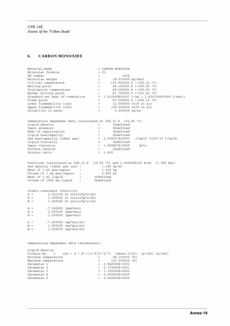
CPR 14EAnnex of the ‘Yellow Book’
Annex-19
6. CARBON MONOXIDE
Material_Name = CARBON MONOXIDEMolecular formula = COUN number = 1016Molecular weight = 28.010000 kg/kmolCritical temperature = 132.920000 K (-140.23 °C)Melting point = 68.150000 K (-205.00 °C)Triplepoint temperature = 68.150000 K (-205.00 °C)Normal boiling point = 81.700000 K (-191.45 °C)Standard net heat of combustion = 1.010400E+0007 J/kg ( 2.830130E+0008 J/kmol)Flash point = 67.050000 K (-206.10 °C)Lower flammability limit = 12.500000 vol% in airUpper flammability limit = 100.000000 vol% in airSolubility in water = 0.000000 kg/m3
Temperature dependent data (calculated at 288.15 K (15.00 °C)Liquid density = UndefinedVapor pressure = UndefinedHeat of vaporization = UndefinedLiquid heatcapacity = UndefinedGas heatcapacity (ideal gas) = 1.039527E+0003 J/kg*K (1039.53 J/kg*K)Liquid viscosity = UndefinedVapor viscosity = 1.668827E-0005 Pa*s Surface tension = UndefinedPoisson ratio = 1.400
Functions (calculated at 288.15 K (15.00 °C) and 1.000000E+05 N/m2 (1.000 Bar)Gas density (ideal gas law) : 1.169 kg/m3Mass of 1 m3 gas/vapour : 1.169 kgVolume of 1 kg gas/vapour : 0.855 m3Mass of 1 m3 liquid : UndefinedVolume of 1000 kg liquid : Undefined
Probit constants (Toxicity)A = 2.321166 SI units(Kg*s/m3)B = 1.000000 SI units(Kg*s/m3)N = 1.000000 SI units(Kg*s/m3)
A = -7.245492 (ppm*min)B = 1.000000 (ppm*min)N = 1.000000 (ppm*min)
A = -7.400000 (mg*min/m3)B = 1.000000 (mg*min/m3)N = 1.000000 (mg*min/m3)
Temperature dependent data (Parameters):
Liquid densityFormula Nr. 1 rho = A * B^-((1-T/C)^2/7) (where C=Tc) [g/cm3] [g/cm3]Minimum temperature = 68.150000 [K]Maximum temperature = 132.920000 [K]Parameter 1 = 2.942500E-0001Parameter 2 = 2.733800E-0001Parameter 3 = 1.329200E+0002Parameter 4 = 0.000000E+0000Parameter 5 = 0.000000E+0000

Annex-20
Vapor pressureFormula Nr. 2 Log(P) = A + B/T + C*Log(T) + D*T + E*T^2 [mm Hg] [mm Hg]Minimum temperature = 68.150000 [K]Maximum temperature = 132.920000 [K]Parameter 1 = 4.611950E+0001Parameter 2 = -7.443300E+0002Parameter 3 = -1.949400E+0001Parameter 4 = 3.642400E-0002Parameter 5 = 2.554400E-0005
Heat of vaporizationFormula Nr. 3 Hv = A * ((C-T)/(C-B)^D (A=Hv1, B=T1, C=Tc) [cal/g] [cal/g]Minimum temperature = 68.150000 [K]Maximum temperature = 132.920000 [K]Parameter 1 = 4.356000E+0001Parameter 2 = 1.005000E+0002Parameter 3 = 1.329200E+0002Parameter 4 = 3.180000E-0001Parameter 5 = 0.000000E+0000
Liquid heatcapacityFormula Nr. 4 Cpl = A + B*T + C*T^2 + D*T^3 [cal/g/K] [cal/g/K]Minimum temperature = 68.150000 [K]Maximum temperature = 90.000000 [K]Parameter 1 = 4.702800E-0001Parameter 2 = 6.002600E-0004Parameter 3 = 2.323900E-0009Parameter 4 = -1.043000E-0011Parameter 5 = 0.000000E+0000
IG heatcapacityFormula Nr. 5 Cp = A + B*T + C*T^2 + D*T^3 [cal/mol] [cal/mol]Minimum temperature = 170.000000 [K]Maximum temperature = 1100.000000 [K]Parameter 1 = 7.045700E+0000Parameter 2 = -1.196000E-0003Parameter 3 = 3.472100E-0006Parameter 4 = -1.401000E-0009Parameter 5 = 0.000000E+0000
Liquid viscosityFormula Nr. 6 Log(Visc) = Ea + Eb/T + Ec*Log (T) + Ed*T + Ee*T*T (where Ec=0!) [centiPoise][centiPoise]Minimum temperature = 68.550000 [K]Maximum temperature = 131.370000 [K]Parameter 1 = -1.366300E+0000Parameter 2 = 6.540800E+0001Parameter 3 = 0.000000E+0000Parameter 4 = -2.344000E-0003Parameter 5 = -6.416000E-0007
Vapor viscosityFormula Nr. 7 Visc = A + B*T + C*T^2 [microPoise] [microPoise]Minimum temperature = 68.150000 [K]Maximum temperature = 1250.000000 [K]Parameter 1 = 1.283800E+0001Parameter 2 = 5.909900E-0001Parameter 3 = -1.957000E-0004Parameter 4 = 0.000000E+0000Parameter 5 = 0.000000E+0000
Surface TensionFormula Nr. 8 Sigma = A * ((C-T)/(C-B))^D (A=Sigma1, B=T1, C=Tc) [dynes/cm] [dynes/cm]Minimum temperature = 68.150000 [K]Maximum temperature = 132.920000 [K]Parameter 1 = 5.646000E+0000Parameter 2 = 1.005000E+0002Parameter 3 = 1.329200E+0002Parameter 4 = 1.133000E+0000Parameter 5 = 0.000000E+0000
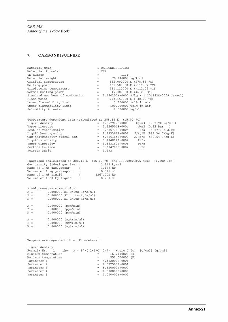
CPR 14EAnnex of the ‘Yellow Book’
Annex-21
7. CARBONDISULFIDE
Material_Name = CARBONDISULFIDEMolecular formula = CS2UN number = 1131Molecular weight = 76.140000 kg/kmolCritical temperature = 552.000000 K (278.85 °C)Melting point = 161.580000 K (-111.57 °C)Triplepoint temperature = 161.110000 K (-112.04 °C)Normal boiling point = 319.380000 K (46.23 °C)Standard net heat of combustion = 1.450200E+0007 J/kg ( 1.104182E+0009 J/kmol)Flash point = 243.150000 K (-30.00 °C)Lower flammability limit = 1.300000 vol% in airUpper flammability limit = 100.000000 vol% in airSolubility in water = 2.000000 kg/m3
Temperature dependent data (calculated at 288.15 K (15.00 °C)Liquid density = 1.267902E+0003 kg/m3 (1267.90 kg/m3 )Vapor pressure = 3.226504E+0004 N/m2 (0.32 Bar )Heat of vaporization = 3.685778E+0005 J/kg (368577.84 J/kg )Liquid heatcapacity = 9.993362E+0002 J/kg*K (999.34 J/kg*K)Gas heatcapacity (ideal gas) = 5.806365E+0002 J/kg*K (580.64 J/kg*K)Liquid viscosity = 3.794892E-0004 Pa*s Vapor viscosity = 9.563160E-0006 Pa*s Surface tension = 3.304700E-0002 N/m Poisson ratio = 1.232
Functions (calculated at 288.15 K (15.00 °C) and 1.000000E+05 N/m2 (1.000 Bar)Gas density (ideal gas law) : 3.178 kg/m3Mass of 1 m3 gas/vapour : 3.178 kgVolume of 1 kg gas/vapour : 0.315 m3Mass of 1 m3 liquid : 1267.902 kgVolume of 1000 kg liquid : 0.789 m3
Probit constants (Toxicity)A = 0.000000 SI units(Kg*s/m3)B = 0.000000 SI units(Kg*s/m3)N = 0.000000 SI units(Kg*s/m3)
A = 0.000000 (ppm*min)B = 0.000000 (ppm*min)N = 0.000000 (ppm*min)
A = 0.000000 (mg*min/m3)B = 0.000000 (mg*min/m3)N = 0.000000 (mg*min/m3)
Temperature dependent data (Parameters):
Liquid densityFormula Nr. 1 rho = A * B^-((1-T/C)^2/7) (where C=Tc) [g/cm3] [g/cm3]Minimum temperature = 161.110000 [K]Maximum temperature = 552.000000 [K]Parameter 1 = 4.302000E-0001Parameter 2 = 2.632500E-0001Parameter 3 = 5.520000E+0002Parameter 4 = 0.000000E+0000Parameter 5 = 0.000000E+0000

Annex-22
Vapor pressureFormula Nr. 2 Log(P) = A + B/T + C*Log(T) + D*T + E*T^2 [mm Hg] [mm Hg]Minimum temperature = 161.110000 [K]Maximum temperature = 552.000000 [K]Parameter 1 = 2.097620E+0001Parameter 2 = -1.969200E+0003Parameter 3 = -4.912400E+0000Parameter 4 = 6.857900E-0004Parameter 5 = 1.525500E-0006
Heat of vaporizationFormula Nr. 3 Hv = A * ((C-T)/(C-B)^D (A=Hv1, B=T1, C=Tc) [cal/g] [cal/g]Minimum temperature = 161.110000 [K]Maximum temperature = 552.000000 [K]Parameter 1 = 8.050000E+0001Parameter 2 = 3.566000E+0002Parameter 3 = 5.520000E+0002Parameter 4 = 2.985000E-0001Parameter 5 = 0.000000E+0000
Liquid heatcapacityFormula Nr. 4 Cpl = A + B*T + C*T^2 + D*T^3 [cal/g/K] [cal/g/K]Minimum temperature = 163.930000 [K]Maximum temperature = 552.000000 [K]Parameter 1 = 1.944500E-0001Parameter 2 = 5.827900E-0004Parameter 3 = -2.731000E-0006Parameter 4 = 4.309600E-0009Parameter 5 = 0.000000E+0000
IG heatcapacityFormula Nr. 5 Cp = A + B*T + C*T^2 + D*T^3 [cal/mol] [cal/mol]Minimum temperature = 100.000000 [K]Maximum temperature = 773.000000 [K]Parameter 1 = 5.595400E+0000Parameter 2 = 2.258400E-0002Parameter 3 = -2.040000E-0005Parameter 4 = 6.359600E-0009Parameter 5 = 0.000000E+0000
Liquid viscosityFormula Nr. 6 Log(Visc) = Ea + Eb/T + Ec*Log (T) + Ed*T + Ee*T*T (where Ec=0!) [centiPoise][centiPoise]Minimum temperature = 235.000000 [K]Maximum temperature = 320.000000 [K]Parameter 1 = -3.665800E+0000Parameter 2 = 6.549200E+0002Parameter 3 = 0.000000E+0000Parameter 4 = 2.539300E-0003Parameter 5 = 2.896000E-0006
Vapor viscosityFormula Nr. 7 Visc = A + B*T + C*T^2 [microPoise] [microPoise]Minimum temperature = 273.150000 [K]Maximum temperature = 582.950000 [K]Parameter 1 = -7.759100E+0000Parameter 2 = 3.662400E-0001Parameter 3 = -2.579000E-0005Parameter 4 = 0.000000E+0000Parameter 5 = 0.000000E+0000
Surface TensionFormula Nr. 8 Sigma = A * ((C-T)/(C-B))^D (A=Sigma1, B=T1, C=Tc) [dynes/cm] [dynes/cm]Minimum temperature = 161.110000 [K]Maximum temperature = 552.000000 [K]Parameter 1 = 2.311000E+0001Parameter 2 = 3.566000E+0002Parameter 3 = 5.520000E+0002Parameter 4 = 1.190900E+0000Parameter 5 = 0.000000E+0000

CPR 14EAnnex of the ‘Yellow Book’
Annex-23
8. CHLORINE
Material_Name = CHLORINEMolecular formula = Cl2UN number = 1017Molecular weight = 70.910000 kg/kmolCritical temperature = 417.150000 K (144.00 °C)Melting point = 172.120000 K (-101.03 °C)Triplepoint temperature = 172.120000 K (-101.03 °C)Normal boiling point = 239.120000 K (-34.03 °C)Standard net heat of combustion = 0.000000E+0000 J/kg ( 0.000000E+0000 J/kmol)Flash point = 0.000000 K (-273.15 °C)Lower flammability limit = 0.000000 vol% in airUpper flammability limit = 0.000000 vol% in airSolubility in water = 7.000000 kg/m3
Temperature dependent data (calculated at 288.15 K (15.00 °C)Liquid density = 1.427436E+0003 kg/m3 (1427.44 kg/m3 )Vapor pressure = 5.889504E+0005 N/m2 (5.89 Bar )Heat of vaporization = 2.565440E+0005 J/kg (256544.02 J/kg )Liquid heatcapacity = 8.994889E+0002 J/kg*K (899.49 J/kg*K)Gas heatcapacity (ideal gas) = 4.714603E+0002 J/kg*K (471.46 J/kg*K)Liquid viscosity = 3.405445E-0004 Pa*s Vapor viscosity = 1.295505E-0005 Pa*s Surface tension = 1.890329E-0002 N/m Poisson ratio = 1.331
Functions (calculated at 288.15 K (15.00 °C) and 1.000000E+05 N/m2 (1.000 Bar)Gas density (ideal gas law) : 2.960 kg/m3Mass of 1 m3 gas/vapour : 2.960 kgVolume of 1 kg gas/vapour : 0.338 m3Mass of 1 m3 liquid : 1427.436 kgVolume of 1000 kg liquid : 0.701 m3
Probit constants (Toxicity)A = 10.599000 SI units(Kg*s/m3)B = 0.500000 SI units(Kg*s/m3)N = 2.750000 SI units(Kg*s/m3)
A = -4.860538 (ppm*min)B = 0.500000 (ppm*min)N = 2.750000 (ppm*min)
A = -6.350155 (mg*min/m3)B = 0.500000 (mg*min/m3)N = 2.750000 (mg*min/m3)
Temperature dependent data (Parameters):
Liquid densityFormula Nr. 1 rho = A * B^-((1-T/C)^2/7) (where C=Tc) [g/cm3] [g/cm3]Minimum temperature = 172.120000 [K]Maximum temperature = 417.150000 [K]Parameter 1 = 5.624400E-0001Parameter 2 = 2.718800E-0001Parameter 3 = 4.171500E+0002Parameter 4 = 0.000000E+0000Parameter 5 = 0.000000E+0000

Annex-24
Vapor pressureFormula Nr. 2 Log(P) = A + B/T + C*Log(T) + D*T + E*T^2 [mm Hg] [mm Hg]Minimum temperature = 172.120000 [K]Maximum temperature = 417.150000 [K]Parameter 1 = 2.275110E+0001Parameter 2 = -1.570600E+0003Parameter 3 = -5.743400E+0000Parameter 4 = 8.377100E-0004Parameter 5 = 2.769700E-0006
Heat of vaporizationFormula Nr. 3 Hv = A * ((C-T)/(C-B)^D (A=Hv1, B=T1, C=Tc) [cal/g] [cal/g]Minimum temperature = 172.120000 [K]Maximum temperature = 417.150000 [K]Parameter 1 = 6.010000E+0001Parameter 2 = 2.946000E+0002Parameter 3 = 4.171500E+0002Parameter 4 = 3.810400E-0001Parameter 5 = 0.000000E+0000
Liquid heatcapacityFormula Nr. 4 Cpl = A + B*T + C*T^2 + D*T^3 [cal/g/K] [cal/g/K]Minimum temperature = 172.000000 [K]Maximum temperature = 353.000000 [K]Parameter 1 = 2.175900E-0001Parameter 2 = 1.240400E-0004Parameter 3 = -3.898000E-0007Parameter 4 = -2.544000E-0010Parameter 5 = 0.000000E+0000
IG heatcapacityFormula Nr. 5 Cp = A + B*T + C*T^2 + D*T^3 [cal/mol] [cal/mol]Minimum temperature = 100.000000 [K]Maximum temperature = 773.000000 [K]Parameter 1 = 6.351200E+0000Parameter 2 = 7.605900E-0003Parameter 3 = -7.389000E-0006Parameter 4 = 2.387200E-0009Parameter 5 = 0.000000E+0000
Liquid viscosityFormula Nr. 6 Log(Visc) = Ea + Eb/T + Ec*Log (T) + Ed*T + Ee*T*T (where Ec=0!) [centiPoise][centiPoise]Minimum temperature = 190.000000 [K]Maximum temperature = 300.000000 [K]Parameter 1 = -7.674200E+0000Parameter 2 = 6.904900E+0002Parameter 3 = 0.000000E+0000Parameter 4 = 2.860800E-0002Parameter 5 = -4.135000E-0005
Vapor viscosityFormula Nr. 7 Visc = A + B*T + C*T^2 [microPoise] [microPoise]Minimum temperature = 200.000000 [K]Maximum temperature = 1000.000000 [K]Parameter 1 = -5.394300E+0000Parameter 2 = 4.949800E-0001Parameter 3 = -9.254000E-0005Parameter 4 = 0.000000E+0000Parameter 5 = 0.000000E+0000
Surface TensionFormula Nr. 8 Sigma = A * ((C-T)/(C-B))^D (A=Sigma1, B=T1, C=Tc) [dynes/cm] [dynes/cm]Minimum temperature = 172.120000 [K]Maximum temperature = 417.150000 [K]Parameter 1 = 1.788000E+0001Parameter 2 = 2.946000E+0002Parameter 3 = 4.171500E+0002Parameter 4 = 1.085000E+0000Parameter 5 = 0.000000E+0000

CPR 14EAnnex of the ‘Yellow Book’
Annex-25
9. ETHENE
Material_Name = ETHENEMolecular formula = CH2=CH2UN number = 1962Molecular weight = 28.052000 kg/kmolCritical temperature = 282.900000 K (9.75 °C)Melting point = 104.000000 K (-169.15 °C)Triplepoint temperature = 104.000000 K (-169.15 °C)Normal boiling point = 169.300000 K (-103.85 °C)Standard net heat of combustion = 4.719400E+0007 J/kg ( 1.323886E+0009 J/kmol)Flash point = 125.700000 K (-147.45 °C)Lower flammability limit = 2.750000 vol% in airUpper flammability limit = 100.000000 vol% in airSolubility in water = 0.100000 kg/m3
Temperature dependent data (calculated at 288.15 K (15.00 °C)Liquid density = UndefinedVapor pressure = UndefinedHeat of vaporization = UndefinedLiquid heatcapacity = UndefinedGas heatcapacity (ideal gas) = 1.540338E+0003 J/kg*K (1540.34 J/kg*K)Liquid viscosity = UndefinedVapor viscosity = 9.812499E-0006 Pa*s Surface tension = UndefinedPoisson ratio = 1.238
Functions (calculated at 288.15 K (15.00 °C) and 1.000000E+05 N/m2 (1.000 Bar)Gas density (ideal gas law) : 1.171 kg/m3Mass of 1 m3 gas/vapour : 1.171 kgVolume of 1 kg gas/vapour : 0.854 m3Mass of 1 m3 liquid : UndefinedVolume of 1000 kg liquid : Undefined
Probit constants (Toxicity)A = 0.000000 SI units(Kg*s/m3)B = 0.000000 SI units(Kg*s/m3)N = 0.000000 SI units(Kg*s/m3)
A = 0.000000 (ppm*min)B = 0.000000 (ppm*min)N = 0.000000 (ppm*min)
A = 0.000000 (mg*min/m3)B = 0.000000 (mg*min/m3)N = 0.000000 (mg*min/m3)
Temperature dependent data (Parameters):
Liquid densityFormula Nr. 1 rho = A * B^-((1-T/C)^2/7) (where C=Tc) [g/cm3] [g/cm3]Minimum temperature = 103.800000 [K]Maximum temperature = 282.900000 [K]Parameter 1 = 2.118000E-0001Parameter 2 = 2.784000E-0001Parameter 3 = 2.829000E+0002Parameter 4 = 0.000000E+0000Parameter 5 = 0.000000E+0000

Annex-26
Vapor pressureFormula Nr. 2 Log(P) = A + B/T + C*Log(T) + D*T + E*T^2 [mm Hg] [mm Hg]Minimum temperature = 104.000000 [K]Maximum temperature = 283.100000 [K]Parameter 1 = 3.089500E+0001Parameter 2 = -1.196800E+0003Parameter 3 = -1.015300E+0001Parameter 4 = 9.935100E-0003Parameter 5 = 0.000000E+0000
Heat of vaporizationFormula Nr. 3 Hv = A * ((C-T)/(C-B)^D (A=Hv1, B=T1, C=Tc) [cal/g] [cal/g]Minimum temperature = 103.800000 [K]Maximum temperature = 282.900000 [K]Parameter 1 = 1.154000E+0002Parameter 2 = 1.693000E+0002Parameter 3 = 2.829000E+0002Parameter 4 = 3.800000E-0001Parameter 5 = 0.000000E+0000
Liquid heatcapacityFormula Nr. 4 Cpl = A + B*T + C*T^2 + D*T^3 [cal/g/K] [cal/g/K]Minimum temperature = 104.000000 [K]Maximum temperature = 233.000000 [K]Parameter 1 = 3.402000E-0001Parameter 2 = 6.218000E-0003Parameter 3 = -5.012000E-0005Parameter 4 = 1.263000E-0007Parameter 5 = 0.000000E+0000
IG heatcapacityFormula Nr. 5 Cp = A + B*T + C*T^2 + D*T^3 [cal/mol] [cal/mol]Minimum temperature = 298.000000 [K]Maximum temperature = 1500.000000 [K]Parameter 1 = 9.340000E-0001Parameter 2 = 3.690000E-0002Parameter 3 = -1.930000E-0005Parameter 4 = 4.010000E-0009Parameter 5 = 0.000000E+0000
Liquid viscosityFormula Nr. 6 Log(Visc) = Ea + Eb/T + Ec*Log (T) + Ed*T + Ee*T*T (where Ec=0!) [centiPoise][centiPoise]Minimum temperature = 103.800000 [K]Maximum temperature = 282.900000 [K]Parameter 1 = -7.706000E+0000Parameter 2 = 4.681000E+0002Parameter 3 = 0.000000E+0000Parameter 4 = 3.725000E-0002Parameter 5 = -7.633000E-0005
Vapor viscosityFormula Nr. 7 Visc = A + B*T + C*T^2 [microPoise] [microPoise]Minimum temperature = 173.000000 [K]Maximum temperature = 1073.000000 [K]Parameter 1 = 3.586000E+0000Parameter 2 = 3.513000E-0001Parameter 3 = -8.055000E-0005Parameter 4 = 0.000000E+0000Parameter 5 = 0.000000E+0000
Surface TensionFormula Nr. 8 Sigma = A * ((C-T)/(C-B))^D (A=Sigma1, B=T1, C=Tc) [dynes/cm] [dynes/cm]Minimum temperature = 103.800000 [K]Maximum temperature = 282.900000 [K]Parameter 1 = 1.952000E+0001Parameter 2 = 1.530000E+0002Parameter 3 = 2.829000E+0002Parameter 4 = 1.276000E+0000Parameter 5 = 0.000000E+0000
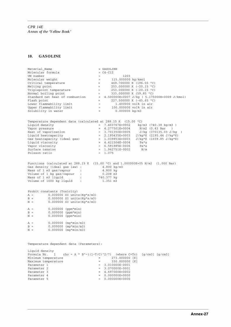
CPR 14EAnnex of the ‘Yellow Book’
Annex-27
10. GASOLINE
Material_Name = GASOLINEMolecular formula = C4-C12UN number = 1203Molecular weight = 115.000000 kg/kmolCritical temperature = 469.700000 K (196.55 °C)Melting point = 253.000000 K (-20.15 °C)Triplepoint temperature = 253.000000 K (-20.15 °C)Normal boiling point = 333.000000 K (59.85 °C)Standard net heat of combustion = 4.500000E+0007 J/kg ( 5.175000E+0009 J/kmol)Flash point = 227.500000 K (-45.65 °C)Lower flammability limit = 1.400000 vol% in airUpper flammability limit = 100.000000 vol% in airSolubility in water = 0.000000 kg/m3
Temperature dependent data (calculated at 288.15 K (15.00 °C)Liquid density = 7.403767E+0002 kg/m3 (740.38 kg/m3 )Vapor pressure = 4.277501E+0004 N/m2 (0.43 Bar )Heat of vaporization = 3.701350E+0005 J/kg (370135.03 J/kg )Liquid heatcapacity = 2.195435E+0003 J/kg*K (2195.44 J/kg*K)Gas heatcapacity (ideal gas) = 1.039853E+0003 J/kg*K (1039.85 J/kg*K)Liquid viscosity = 4.421504E-0004 Pa*s Vapor viscosity = 6.591885E-0006 Pa*s Surface tension = 1.962751E-0002 N/m Poisson ratio = 1.075
Functions (calculated at 288.15 K (15.00 °C) and 1.000000E+05 N/m2 (1.000 Bar)Gas density (ideal gas law) : 4.800 kg/m3Mass of 1 m3 gas/vapour : 4.800 kgVolume of 1 kg gas/vapour : 0.208 m3Mass of 1 m3 liquid : 740.377 kgVolume of 1000 kg liquid : 1.351 m3
Probit constants (Toxicity)A = 0.000000 SI units(Kg*s/m3)B = 0.000000 SI units(Kg*s/m3)N = 0.000000 SI units(Kg*s/m3)
A = 0.000000 (ppm*min)B = 0.000000 (ppm*min)N = 0.000000 (ppm*min)
A = 0.000000 (mg*min/m3)B = 0.000000 (mg*min/m3)N = 0.000000 (mg*min/m3)
Temperature dependent data (Parameters):
Liquid densityFormula Nr. 1 rho = A * B^-((1-T/C)^2/7) (where C=Tc) [g/cm3] [g/cm3]Minimum temperature = 273.000000 [K]Maximum temperature = 330.000000 [K]Parameter 1 = 3.010000E-0001Parameter 2 = 3.070000E-0001Parameter 3 = 4.697000E+0002Parameter 4 = 0.000000E+0000Parameter 5 = 0.000000E+0000

Annex-28
Vapor pressureFormula Nr. 2 Log(P) = A + B/T + C*Log(T) + D*T + E*T^2 [mm Hg] [mm Hg]Minimum temperature = 263.000000 [K]Maximum temperature = 343.000000 [K]Parameter 1 = -1.137520E+0001Parameter 2 = 0.000000E+0000Parameter 3 = 0.000000E+0000Parameter 4 = 7.820000E-0002Parameter 5 = -1.042000E-0004
Heat of vaporizationFormula Nr. 3 Hv = A * ((C-T)/(C-B)^D (A=Hv1, B=T1, C=Tc) [cal/g] [cal/g]Minimum temperature = 260.000000 [K]Maximum temperature = 470.000000 [K]Parameter 1 = 8.361200E+0001Parameter 2 = 3.130000E+0002Parameter 3 = 4.697000E+0002Parameter 4 = 3.800000E-0001Parameter 5 = 0.000000E+0000
Liquid heatcapacityFormula Nr. 4 Cpl = A + B*T + C*T^2 + D*T^3 [cal/g/K] [cal/g/K]Minimum temperature = 240.000000 [K]Maximum temperature = 330.000000 [K]Parameter 1 = 2.713000E-0001Parameter 2 = 1.000000E-0003Parameter 3 = -4.212800E-0007Parameter 4 = 0.000000E+0000Parameter 5 = 0.000000E+0000
IG heatcapacityFormula Nr. 5 Cp = A + B*T + C*T^2 + D*T^3 [cal/mol] [cal/mol]Minimum temperature = 200.000000 [K]Maximum temperature = 1500.000000 [K]Parameter 1 = 3.077910E+0000Parameter 2 = 9.977430E-0002Parameter 3 = -4.079680E-0005Parameter 4 = 5.303310E-0009Parameter 5 = 0.000000E+0000
Liquid viscosityFormula Nr. 6 Log(Visc) = Ea + Eb/T + Ec*Log (T) + Ed*T + Ee*T*T (where Ec=0!) [centiPoise][centiPoise]Minimum temperature = 273.000000 [K]Maximum temperature = 330.000000 [K]Parameter 1 = 2.233000E+0000Parameter 2 = 0.000000E+0000Parameter 3 = 0.000000E+0000Parameter 4 = -1.310000E-0002Parameter 5 = 1.430000E-0005
Vapor viscosityFormula Nr. 7 Visc = A + B*T + C*T^2 [microPoise] [microPoise]Minimum temperature = 250.000000 [K]Maximum temperature = 600.000000 [K]Parameter 1 = -8.111910E+0000Parameter 2 = 2.729870E-0001Parameter 3 = -5.576810E-0005Parameter 4 = 0.000000E+0000Parameter 5 = 0.000000E+0000
Surface TensionFormula Nr. 8 Sigma = A * ((C-T)/(C-B))^D (A=Sigma1, B=T1, C=Tc) [dynes/cm] [dynes/cm]Minimum temperature = 273.000000 [K]Maximum temperature = 330.000000 [K]Parameter 1 = 1.900000E+0001Parameter 2 = 2.930000E+0002Parameter 3 = 4.697000E+0002Parameter 4 = 1.200000E+0000Parameter 5 = 0.000000E+0000
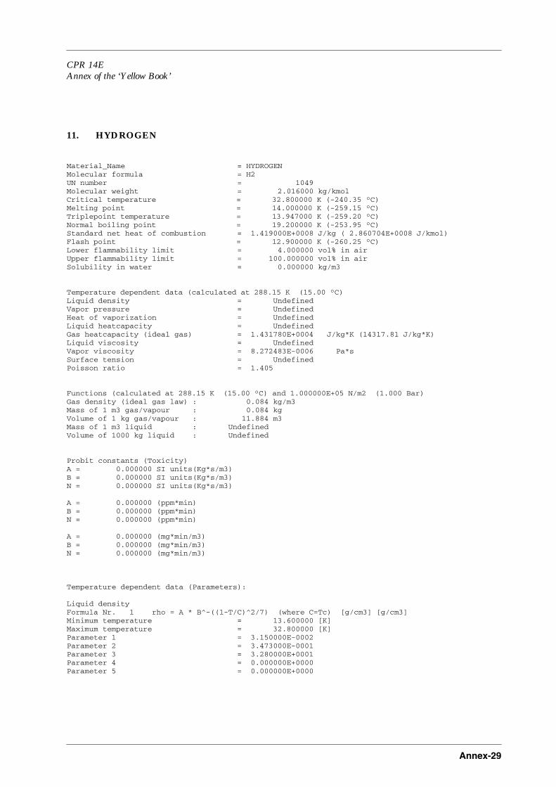
CPR 14EAnnex of the ‘Yellow Book’
Annex-29
11. HYDROGEN
Material_Name = HYDROGENMolecular formula = H2UN number = 1049Molecular weight = 2.016000 kg/kmolCritical temperature = 32.800000 K (-240.35 °C)Melting point = 14.000000 K (-259.15 °C)Triplepoint temperature = 13.947000 K (-259.20 °C)Normal boiling point = 19.200000 K (-253.95 °C)Standard net heat of combustion = 1.419000E+0008 J/kg ( 2.860704E+0008 J/kmol)Flash point = 12.900000 K (-260.25 °C)Lower flammability limit = 4.000000 vol% in airUpper flammability limit = 100.000000 vol% in airSolubility in water = 0.000000 kg/m3
Temperature dependent data (calculated at 288.15 K (15.00 °C)Liquid density = UndefinedVapor pressure = UndefinedHeat of vaporization = UndefinedLiquid heatcapacity = UndefinedGas heatcapacity (ideal gas) = 1.431780E+0004 J/kg*K (14317.81 J/kg*K)Liquid viscosity = UndefinedVapor viscosity = 8.272483E-0006 Pa*s Surface tension = UndefinedPoisson ratio = 1.405
Functions (calculated at 288.15 K (15.00 °C) and 1.000000E+05 N/m2 (1.000 Bar)Gas density (ideal gas law) : 0.084 kg/m3Mass of 1 m3 gas/vapour : 0.084 kgVolume of 1 kg gas/vapour : 11.884 m3Mass of 1 m3 liquid : UndefinedVolume of 1000 kg liquid : Undefined
Probit constants (Toxicity)A = 0.000000 SI units(Kg*s/m3)B = 0.000000 SI units(Kg*s/m3)N = 0.000000 SI units(Kg*s/m3)
A = 0.000000 (ppm*min)B = 0.000000 (ppm*min)N = 0.000000 (ppm*min)
A = 0.000000 (mg*min/m3)B = 0.000000 (mg*min/m3)N = 0.000000 (mg*min/m3)
Temperature dependent data (Parameters):
Liquid densityFormula Nr. 1 rho = A * B^-((1-T/C)^2/7) (where C=Tc) [g/cm3] [g/cm3]Minimum temperature = 13.600000 [K]Maximum temperature = 32.800000 [K]Parameter 1 = 3.150000E-0002Parameter 2 = 3.473000E-0001Parameter 3 = 3.280000E+0001Parameter 4 = 0.000000E+0000Parameter 5 = 0.000000E+0000

Annex-30
Vapor pressureFormula Nr. 2 Log(P) = A + B/T + C*Log(T) + D*T + E*T^2 [mm Hg] [mm Hg]Minimum temperature = 13.600000 [K]Maximum temperature = 32.800000 [K]Parameter 1 = 5.236600E+0000Parameter 2 = -4.628000E+0001Parameter 3 = -4.480900E-0001Parameter 4 = 2.529000E-0002Parameter 5 = 0.000000E+0000
Heat of vaporizationFormula Nr. 3 Hv = A * ((C-T)/(C-B)^D (A=Hv1, B=T1, C=Tc) [cal/g] [cal/g]Minimum temperature = 13.600000 [K]Maximum temperature = 32.800000 [K]Parameter 1 = 1.070000E+0002Parameter 2 = 2.020000E+0001Parameter 3 = 3.280000E+0001Parameter 4 = 2.370000E-0001Parameter 5 = 0.000000E+0000
Liquid heatcapacityFormula Nr. 4 Cpl = A + B*T + C*T^2 + D*T^3 [cal/g/K] [cal/g/K]Minimum temperature = 13.600000 [K]Maximum temperature = 28.000000 [K]Parameter 1 = 3.790000E+0000Parameter 2 = -3.298000E-0001Parameter 3 = 1.217090E-0002Parameter 4 = -2.434800E-0006Parameter 5 = 0.000000E+0000
IG heatcapacityFormula Nr. 5 Cp = A + B*T + C*T^2 + D*T^3 [cal/mol] [cal/mol]Minimum temperature = 298.000000 [K]Maximum temperature = 1500.000000 [K]Parameter 1 = 6.880000E+0000Parameter 2 = -2.200000E-0005Parameter 3 = 2.100000E-0007Parameter 4 = 1.300000E-0010Parameter 5 = 0.000000E+0000
Liquid viscosityFormula Nr. 6 Log(Visc) = Ea + Eb/T + Ec*Log (T) + Ed*T + Ee*T*T (where Ec=0!) [centiPoise][centiPoise]Minimum temperature = 13.600000 [K]Maximum temperature = 32.800000 [K]Parameter 1 = -4.857000E+0000Parameter 2 = 2.513000E+0001Parameter 3 = 0.000000E+0000Parameter 4 = 1.409000E-0001Parameter 5 = -2.773000E-0003
Vapor viscosityFormula Nr. 7 Visc = A + B*T + C*T^2 [microPoise] [microPoise]Minimum temperature = 113.000000 [K]Maximum temperature = 1473.000000 [K]Parameter 1 = 2.187000E+0001Parameter 2 = 2.220000E-0001Parameter 3 = -3.751000E-0005Parameter 4 = 0.000000E+0000Parameter 5 = 0.000000E+0000
Surface TensionFormula Nr. 8 Sigma = A * ((C-T)/(C-B))^D (A=Sigma1, B=T1, C=Tc) [dynes/cm] [dynes/cm]Minimum temperature = 13.600000 [K]Maximum temperature = 32.800000 [K]Parameter 1 = 2.410000E+0000Parameter 2 = 1.700000E+0001Parameter 3 = 3.280000E+0001Parameter 4 = 1.101200E+0000Parameter 5 = 0.000000E+0000

CPR 14EAnnex of the ‘Yellow Book’
Annex-31
12. HYDROGEN CHLORIDE
Material_Name = HYDROGEN CHLORIDEMolecular formula = HClUN number = 1050Molecular weight = 36.460000 kg/kmolCritical temperature = 324.650000 K (51.50 °C)Melting point = 158.970000 K (-114.18 °C)Triplepoint temperature = 158.970000 K (-114.18 °C)Normal boiling point = 188.150000 K (-85.00 °C)Standard net heat of combustion = 7.844600E+0005 J/kg ( 2.860141E+0007 J/kmol)Flash point = 0.000000 K (-273.15 °C)Lower flammability limit = 0.000000 vol% in airUpper flammability limit = 0.000000 vol% in airSolubility in water = 720.000000 kg/m3
Temperature dependent data (calculated at 288.15 K (15.00 °C)Liquid density = 8.469085E+0002 kg/m3 (846.91 kg/m3 )Vapor pressure = 3.728652E+0006 N/m2 (37.29 Bar )Heat of vaporization = 2.757109E+0005 J/kg (275710.86 J/kg )Liquid heatcapacity = 1.753942E+0003 J/kg*K (1753.94 J/kg*K)Gas heatcapacity (ideal gas) = 7.957981E+0002 J/kg*K (795.80 J/kg*K)Liquid viscosity = 9.022553E-0005 Pa*s Vapor viscosity = 1.413966E-0005 Pa*s Surface tension = 5.004225E-0003 N/m Poisson ratio = 1.402
Functions (calculated at 288.15 K (15.00 °C) and 1.000000E+05 N/m2 (1.000 Bar)Gas density (ideal gas law) : 1.522 kg/m3Mass of 1 m3 gas/vapour : 1.522 kgVolume of 1 kg gas/vapour : 0.657 m3Mass of 1 m3 liquid : 846.909 kgVolume of 1000 kg liquid : 1.181 m3
Probit constants (Toxicity)A = -1.428900 SI units(Kg*s/m3)B = 3.690000 SI units(Kg*s/m3)N = 1.000000 SI units(Kg*s/m3)
A = -35.756985 (ppm*min)B = 3.690000 (ppm*min)N = 1.000000 (ppm*min)
A = -37.300003 (mg*min/m3)B = 3.690000 (mg*min/m3)N = 1.000000 (mg*min/m3)
Temperature dependent data (Parameters):
Liquid densityFormula Nr. 1 rho = A * B^-((1-T/C)^2/7) (where C=Tc) [g/cm3] [g/cm3]Minimum temperature = 158.970000 [K]Maximum temperature = 324.650000 [K]Parameter 1 = 4.023500E-0001Parameter 2 = 2.491600E-0001Parameter 3 = 3.246500E+0002Parameter 4 = 0.000000E+0000Parameter 5 = 0.000000E+0000

Annex-32
Vapor pressureFormula Nr. 2 Log(P) = A + B/T + C*Log(T) + D*T + E*T^2 [mm Hg] [mm Hg]Minimum temperature = 158.970000 [K]Maximum temperature = 324.650000 [K]Parameter 1 = 3.085270E+0001Parameter 2 = -1.435900E+0003Parameter 3 = -9.269400E+0000Parameter 4 = 2.414900E-0003Parameter 5 = 8.196100E-0006
Heat of vaporizationFormula Nr. 3 Hv = A * ((C-T)/(C-B)^D (A=Hv1, B=T1, C=Tc) [cal/g] [cal/g]Minimum temperature = 158.970000 [K]Maximum temperature = 324.650000 [K]Parameter 1 = 9.041000E+0001Parameter 2 = 2.418000E+0002Parameter 3 = 3.246500E+0002Parameter 4 = 3.864100E-0001Parameter 5 = 0.000000E+0000
Liquid heatcapacityFormula Nr. 4 Cpl = A + B*T + C*T^2 + D*T^3 [cal/g/K] [cal/g/K]Minimum temperature = 165.000000 [K]Maximum temperature = 185.000000 [K]Parameter 1 = 3.101300E-0001Parameter 2 = 5.859200E-0004Parameter 3 = 2.148400E-0008Parameter 4 = -4.085000E-0011Parameter 5 = 0.000000E+0000
IG heatcapacityFormula Nr. 5 Cp = A + B*T + C*T^2 + D*T^3 [cal/mol] [cal/mol]Minimum temperature = 273.000000 [K]Maximum temperature = 1500.000000 [K]Parameter 1 = 7.075800E+0000Parameter 2 = -1.102000E-0003Parameter 3 = 2.292800E-0006Parameter 4 = -7.206000E-0010Parameter 5 = 0.000000E+0000
Liquid viscosityFormula Nr. 6 Log(Visc) = Ea + Eb/T + Ec*Log (T) + Ed*T + Ee*T*T (where Ec=0!) [centiPoise][centiPoise]Minimum temperature = 233.150000 [K]Maximum temperature = 313.150000 [K]Parameter 1 = 2.002600E+0000Parameter 2 = -2.604000E+0002Parameter 3 = 0.000000E+0000Parameter 4 = -5.924000E-0003Parameter 5 = -5.258000E-0006
Vapor viscosityFormula Nr. 7 Visc = A + B*T + C*T^2 [microPoise] [microPoise]Minimum temperature = 200.000000 [K]Maximum temperature = 1000.000000 [K]Parameter 1 = -1.125000E+0001Parameter 2 = 5.642100E-0001Parameter 3 = -1.196000E-0004Parameter 4 = 0.000000E+0000Parameter 5 = 0.000000E+0000
Surface TensionFormula Nr. 8 Sigma = A * ((C-T)/(C-B))^D (A=Sigma1, B=T1, C=Tc) [dynes/cm] [dynes/cm]Minimum temperature = 158.970000 [K]Maximum temperature = 324.650000 [K]Parameter 1 = 1.449000E+0001Parameter 2 = 2.418000E+0002Parameter 3 = 3.246500E+0002Parameter 4 = 1.297000E+0000Parameter 5 = 0.000000E+0000

CPR 14EAnnex of the ‘Yellow Book’
Annex-33
13. HYDROGEN CYANIDE
Material_Name = HYDROGEN CYANIDEMolecular formula = HCNUN number = 1051Molecular weight = 27.030000 kg/kmolCritical temperature = 456.650000 K (183.50 °C)Melting point = 259.910000 K (-13.24 °C)Triplepoint temperature = 259.830000 K (-13.32 °C)Normal boiling point = 298.850000 K (25.70 °C)Standard net heat of combustion = 2.306300E+0007 J/kg ( 6.233929E+0008 J/kmol)Flash point = 255.370000 K (-17.78 °C)Lower flammability limit = 6.000000 vol% in airUpper flammability limit = 100.000000 vol% in airSolubility in water = 100.000000 kg/m3
Temperature dependent data (calculated at 288.15 K (15.00 °C)Liquid density = 6.945373E+0002 kg/m3 (694.54 kg/m3 )Vapor pressure = 6.700760E+0004 N/m2 (0.67 Bar )Heat of vaporization = 1.048359E+0006 J/kg (1048359.52 J/kg )Liquid heatcapacity = 2.616330E+0003 J/kg*K (2616.33 J/kg*K)Gas heatcapacity (ideal gas) = 1.311660E+0003 J/kg*K (1311.66 J/kg*K)Liquid viscosity = 2.011130E-0004 Pa*s Vapor viscosity = 2.574882E-0006 Pa*s Surface tension = 1.888982E-0002 N/m Poisson ratio = 1.306
Functions (calculated at 288.15 K (15.00 °C) and 1.000000E+05 N/m2 (1.000 Bar)Gas density (ideal gas law) : 1.128 kg/m3Mass of 1 m3 gas/vapour : 1.128 kgVolume of 1 kg gas/vapour : 0.886 m3Mass of 1 m3 liquid : 694.537 kgVolume of 1000 kg liquid : 1.440 m3
Probit constants (Toxicity)A = 19.262881 SI units(Kg*s/m3)B = 1.000000 SI units(Kg*s/m3)N = 2.400000 SI units(Kg*s/m3)
A = -9.514656 (ppm*min)B = 1.000000 (ppm*min)N = 2.400000 (ppm*min)
A = -9.800000 (mg*min/m3)B = 1.000000 (mg*min/m3)N = 2.400000 (mg*min/m3)
Temperature dependent data (Parameters):
Liquid densityFormula Nr. 1 rho = A * B^-((1-T/C)^2/7) (where C=Tc) [g/cm3] [g/cm3]Minimum temperature = 259.830000 [K]Maximum temperature = 456.650000 [K]Parameter 1 = 1.974900E-0001Parameter 2 = 1.878700E-0001Parameter 3 = 4.566500E+0002Parameter 4 = 0.000000E+0000Parameter 5 = 0.000000E+0000

Annex-34
Vapor pressureFormula Nr. 2 Log(P) = A + B/T + C*Log(T) + D*T + E*T^2 [mm Hg] [mm Hg]Minimum temperature = 259.830000 [K]Maximum temperature = 456.650000 [K]Parameter 1 = 2.928310E+0001Parameter 2 = -2.196200E+0003Parameter 3 = -7.854800E+0000Parameter 4 = -4.266000E-0004Parameter 5 = 5.813000E-0006
Heat of vaporizationFormula Nr. 3 Hv = A * ((C-T)/(C-B)^D (A=Hv1, B=T1, C=Tc) [cal/g] [cal/g]Minimum temperature = 259.830000 [K]Maximum temperature = 456.650000 [K]Parameter 1 = 2.177000E+0002Parameter 2 = 3.582000E+0002Parameter 3 = 4.566500E+0002Parameter 4 = 2.607400E-0001Parameter 5 = 0.000000E+0000
Liquid heatcapacityFormula Nr. 4 Cpl = A + B*T + C*T^2 + D*T^3 [cal/g/K] [cal/g/K]Minimum temperature = 259.830000 [K]Maximum temperature = 298.850000 [K]Parameter 1 = 8.024300E-0001Parameter 2 = -1.307000E-0003Parameter 3 = 1.857500E-0006Parameter 4 = 1.879700E-0009Parameter 5 = 0.000000E+0000
IG heatcapacityFormula Nr. 5 Cp = A + B*T + C*T^2 + D*T^3 [cal/mol] [cal/mol]Minimum temperature = 100.000000 [K]Maximum temperature = 1500.000000 [K]Parameter 1 = 5.683800E+0000Parameter 2 = 1.154300E-0002Parameter 3 = -7.027000E-0006Parameter 4 = 1.807300E-0009Parameter 5 = 0.000000E+0000
Liquid viscosityFormula Nr. 6 Log(Visc) = Ea + Eb/T + Ec*Log (T) + Ed*T + Ee*T*T (where Ec=0!) [centiPoise][centiPoise]Minimum temperature = 259.850000 [K]Maximum temperature = 298.150000 [K]Parameter 1 = -2.410000E+0000Parameter 2 = 4.335200E+0002Parameter 3 = 0.000000E+0000Parameter 4 = 4.523200E-0004Parameter 5 = 9.467600E-0007
Vapor viscosityFormula Nr. 7 Visc = A + B*T + C*T^2 [microPoise] [microPoise]Minimum temperature = 300.000000 [K]Maximum temperature = 425.000000 [K]Parameter 1 = -8.391300E+0000Parameter 2 = 8.982500E-0002Parameter 3 = 7.991800E-0005Parameter 4 = 0.000000E+0000Parameter 5 = 0.000000E+0000
Surface TensionFormula Nr. 8 Sigma = A * ((C-T)/(C-B))^D (A=Sigma1, B=T1, C=Tc) [dynes/cm] [dynes/cm]Minimum temperature = 259.830000 [K]Maximum temperature = 456.650000 [K]Parameter 1 = 1.092000E+0001Parameter 2 = 3.582000E+0002Parameter 3 = 4.566500E+0002Parameter 4 = 1.019800E+0000Parameter 5 = 0.000000E+0000

CPR 14EAnnex of the ‘Yellow Book’
Annex-35
14. HYDROGEN FLUORIDE
Material_Name = HYDROGEN FLUORIDEMolecular formula = HFUN number = 1052Molecular weight = 20.010000 kg/kmolCritical temperature = 461.150000 K (188.00 °C)Melting point = 189.790000 K (-83.36 °C)Triplepoint temperature = 189.790000 K (-83.36 °C)Normal boiling point = 292.670000 K (19.52 °C)Standard net heat of combustion = 1.811600E+0003 J/kg ( 3.625012E+0004 J/kmol)Flash point = 0.000000 K (-273.15 °C)Lower flammability limit = 0.000000 vol% in airUpper flammability limit = 0.000000 vol% in airSolubility in water = 1000.000000 kg/m3
Temperature dependent data (calculated at 288.15 K (15.00 °C)Liquid density = 9.672703E+0002 kg/m3 (967.27 kg/m3 )Vapor pressure = 8.575827E+0004 N/m2 (0.86 Bar )Heat of vaporization = 3.783930E+0005 J/kg (378393.05 J/kg )Liquid heatcapacity = 2.489282E+0003 J/kg*K (2489.28 J/kg*K)Gas heatcapacity (ideal gas) = 1.453429E+0003 J/kg*K (1453.43 J/kg*K)Liquid viscosity = 2.225353E-0004 Pa*s Vapor viscosity = 1.071795E-0005 Pa*s Surface tension = 9.138491E-0003 N/m Poisson ratio = 1.400
Functions (calculated at 288.15 K (15.00 °C) and 1.000000E+05 N/m2 (1.000 Bar)Gas density (ideal gas law) : 0.835 kg/m3Mass of 1 m3 gas/vapour : 0.835 kgVolume of 1 kg gas/vapour : 1.197 m3Mass of 1 m3 liquid : 967.270 kgVolume of 1000 kg liquid : 1.034 m3
Probit constants (Toxicity)A = 8.228900 SI units(Kg*s/m3)B = 1.000000 SI units(Kg*s/m3)N = 1.500000 SI units(Kg*s/m3)
A = -8.672754 (ppm*min)B = 1.000000 (ppm*min)N = 1.500000 (ppm*min)
A = -8.400021 (mg*min/m3)B = 1.000000 (mg*min/m3)N = 1.500000 (mg*min/m3)
Temperature dependent data (Parameters):
Liquid densityFormula Nr. 1 rho = A * B^-((1-T/C)^2/7) (where C=Tc) [g/cm3] [g/cm3]Minimum temperature = 189.790000 [K]Maximum temperature = 461.150000 [K]Parameter 1 = 2.067800E-0001Parameter 2 = 1.298200E-0001Parameter 3 = 4.611500E+0002Parameter 4 = 0.000000E+0000Parameter 5 = 0.000000E+0000

Annex-36
Vapor pressureFormula Nr. 2 Log(P) = A + B/T + C*Log(T) + D*T + E*T^2 [mm Hg] [mm Hg]Minimum temperature = 189.790000 [K]Maximum temperature = 461.150000 [K]Parameter 1 = 2.515930E+0001Parameter 2 = -1.825500E+0003Parameter 3 = -6.813000E+0000Parameter 4 = 9.564300E-0004Parameter 5 = 5.614500E-0006
Heat of vaporizationFormula Nr. 3 Hv = A * ((C-T)/(C-B)^D (A=Hv1, B=T1, C=Tc) [cal/g] [cal/g]Minimum temperature = 181.000000 [K]Maximum temperature = 461.000000 [K]Parameter 1 = 8.948400E+0001Parameter 2 = 2.927000E+0002Parameter 3 = 4.611500E+0002Parameter 4 = 3.800000E-0001Parameter 5 = 0.000000E+0000
Liquid heatcapacityFormula Nr. 4 Cpl = A + B*T + C*T^2 + D*T^3 [cal/g/K] [cal/g/K]Minimum temperature = 189.790000 [K]Maximum temperature = 292.670000 [K]Parameter 1 = 3.073600E-0001Parameter 2 = 9.971000E-0004Parameter 3 = -1.234000E-0010Parameter 4 = 1.820400E-0013Parameter 5 = 0.000000E+0000
IG heatcapacityFormula Nr. 5 Cp = A + B*T + C*T^2 + D*T^3 [cal/mol] [cal/mol]Minimum temperature = 50.000000 [K]Maximum temperature = 1500.000000 [K]Parameter 1 = 7.007700E+0000Parameter 2 = -3.707000E-0004Parameter 3 = 5.620500E-0007Parameter 4 = 6.758700E-0012Parameter 5 = 0.000000E+0000
Liquid viscosityFormula Nr. 6 Log(Visc) = Ea + Eb/T + Ec*Log (T) + Ed*T + Ee*T*T (where Ec=0!) [centiPoise][centiPoise]Minimum temperature = 204.000000 [K]Maximum temperature = 292.670000 [K]Parameter 1 = -4.619600E+0000Parameter 2 = 7.528000E+0002Parameter 3 = 0.000000E+0000Parameter 4 = 3.704700E-0003Parameter 5 = 3.456100E-0006
Vapor viscosityFormula Nr. 7 Visc = A + B*T + C*T^2 [microPoise] [microPoise]Minimum temperature = 285.500000 [K]Maximum temperature = 472.680000 [K]Parameter 1 = -2.158700E+0002Parameter 2 = 1.513000E+0000Parameter 3 = -1.360000E-0003Parameter 4 = 0.000000E+0000Parameter 5 = 0.000000E+0000
Surface TensionFormula Nr. 8 Sigma = A * ((C-T)/(C-B))^D (A=Sigma1, B=T1, C=Tc) [dynes/cm] [dynes/cm]Minimum temperature = 189.790000 [K]Maximum temperature = 461.150000 [K]Parameter 1 = 6.482000E+0000Parameter 2 = 3.255000E+0002Parameter 3 = 4.611500E+0002Parameter 4 = 1.412200E+0000Parameter 5 = 0.000000E+0000

CPR 14EAnnex of the ‘Yellow Book’
Annex-37
15. HYDROGEN SULFIDE
Material_Name = HYDROGEN SULFIDEMolecular formula = H2SUN number = 1053Molecular weight = 34.080000 kg/kmolCritical temperature = 373.530000 K (100.38 °C)Melting point = 187.680000 K (-85.47 °C)Triplepoint temperature = 187.450000 K (-85.70 °C)Normal boiling point = 212.800000 K (-60.35 °C)Standard net heat of combustion = 1.810300E+0007 J/kg ( 6.169502E+0008 J/kmol)Flash point = 166.400000 K (-106.75 °C)Lower flammability limit = 4.300000 vol% in airUpper flammability limit = 100.000000 vol% in airSolubility in water = 6.000000 kg/m3
Temperature dependent data (calculated at 288.15 K (15.00 °C)Liquid density = 7.998392E+0002 kg/m3 (799.84 kg/m3 )Vapor pressure = 1.617544E+0006 N/m2 (16.18 Bar )Heat of vaporization = 4.372398E+0005 J/kg (437239.84 J/kg )Liquid heatcapacity = 2.012115E+0003 J/kg*K (2012.11 J/kg*K)Gas heatcapacity (ideal gas) = 1.006428E+0003 J/kg*K (1006.43 J/kg*K)Liquid viscosity = 4.036770E-0004 Pa*s Vapor viscosity = 1.216139E-0005 Pa*s Surface tension = 1.071192E-0002 N/m Poisson ratio = 1.320
Functions (calculated at 288.15 K (15.00 °C) and 1.000000E+05 N/m2 (1.000 Bar)Gas density (ideal gas law) : 1.422 kg/m3Mass of 1 m3 gas/vapour : 1.422 kgVolume of 1 kg gas/vapour : 0.703 m3Mass of 1 m3 liquid : 799.839 kgVolume of 1000 kg liquid : 1.250 m3
Probit constants (Toxicity)A = 10.655125 SI units(Kg*s/m3)B = 1.000000 SI units(Kg*s/m3)N = 1.900000 SI units(Kg*s/m3)
A = -10.833752 (ppm*min)B = 1.000000 (ppm*min)N = 1.900000 (ppm*min)
A = -11.500000 (mg*min/m3)B = 1.000000 (mg*min/m3)N = 1.900000 (mg*min/m3)
Temperature dependent data (Parameters):
Liquid densityFormula Nr. 1 rho = A * B^-((1-T/C)^2/7) (where C=Tc) [g/cm3] [g/cm3]Minimum temperature = 187.680000 [K]Maximum temperature = 373.530000 [K]Parameter 1 = 3.483400E-0001Parameter 2 = 2.816100E-0001Parameter 3 = 3.735300E+0002Parameter 4 = 0.000000E+0000Parameter 5 = 0.000000E+0000

Annex-38
Vapor pressureFormula Nr. 2 Log(P) = A + B/T + C*Log(T) + D*T + E*T^2 [mm Hg] [mm Hg]Minimum temperature = 187.680000 [K]Maximum temperature = 373.530000 [K]Parameter 1 = 2.003420E+0001Parameter 2 = -1.368500E+0003Parameter 3 = -4.737200E+0000Parameter 4 = 1.039000E-0003Parameter 5 = 1.823500E-0006
Heat of vaporizationFormula Nr. 3 Hv = A * ((C-T)/(C-B)^D (A=Hv1, B=T1, C=Tc) [cal/g] [cal/g]Minimum temperature = 187.680000 [K]Maximum temperature = 373.530000 [K]Parameter 1 = 1.079000E+0002Parameter 2 = 2.806000E+0002Parameter 3 = 3.735300E+0002Parameter 4 = 3.831800E-0001Parameter 5 = 0.000000E+0000
Liquid heatcapacityFormula Nr. 4 Cpl = A + B*T + C*T^2 + D*T^3 [cal/g/K] [cal/g/K]Minimum temperature = 191.480000 [K]Maximum temperature = 208.150000 [K]Parameter 1 = 4.097300E-0001Parameter 2 = 2.715900E-0004Parameter 3 = 3.012300E-0007Parameter 4 = 1.513100E-0010Parameter 5 = 0.000000E+0000
IG heatcapacityFormula Nr. 5 Cp = A + B*T + C*T^2 + D*T^3 [cal/mol] [cal/mol]Minimum temperature = 100.000000 [K]Maximum temperature = 1500.000000 [K]Parameter 1 = 7.757300E+0000Parameter 2 = 1.405700E-0004Parameter 3 = 5.461200E-0006Parameter 4 = -2.403000E-0009Parameter 5 = 0.000000E+0000
Liquid viscosityFormula Nr. 6 Log(Visc) = Ea + Eb/T + Ec*Log (T) + Ed*T + Ee*T*T (where Ec=0!) [centiPoise][centiPoise]Minimum temperature = 190.120000 [K]Maximum temperature = 223.180000 [K]Parameter 1 = -4.638800E+0000Parameter 2 = 5.337700E+0002Parameter 3 = 0.000000E+0000Parameter 4 = 7.180400E-0003Parameter 5 = 5.032300E-0006
Vapor viscosityFormula Nr. 7 Visc = A + B*T + C*T^2 [microPoise] [microPoise]Minimum temperature = 230.000000 [K]Maximum temperature = 570.000000 [K]Parameter 1 = -1.511200E+0001Parameter 2 = 5.113500E-0001Parameter 3 = -1.279000E-0004Parameter 4 = 0.000000E+0000Parameter 5 = 0.000000E+0000
Surface TensionFormula Nr. 8 Sigma = A * ((C-T)/(C-B))^D (A=Sigma1, B=T1, C=Tc) [dynes/cm] [dynes/cm]Minimum temperature = 187.680000 [K]Maximum temperature = 373.530000 [K]Parameter 1 = 1.194000E+0001Parameter 2 = 2.806000E+0002Parameter 3 = 3.735300E+0002Parameter 4 = 1.280900E+0000Parameter 5 = 0.000000E+0000

CPR 14EAnnex of the ‘Yellow Book’
Annex-39
16. METHANE
Material_Name = METHANEMolecular formula = CH4UN number = 1971Molecular weight = 16.043000 kg/kmolCritical temperature = 190.400000 K (-82.75 °C)Melting point = 91.000000 K (-182.15 °C)Triplepoint temperature = 90.670000 K (-182.48 °C)Normal boiling point = 111.500000 K (-161.65 °C)Standard net heat of combustion = 5.002000E+0007 J/kg ( 8.024709E+0008 J/kmol)Flash point = 84.650000 K (-188.50 °C)Lower flammability limit = 5.000000 vol% in airUpper flammability limit = 100.000000 vol% in airSolubility in water = 0.000000 kg/m3
Temperature dependent data (calculated at 288.15 K (15.00 °C)Liquid density = UndefinedVapor pressure = UndefinedHeat of vaporization = UndefinedLiquid heatcapacity = UndefinedGas heatcapacity (ideal gas) = 2.208183E+0003 J/kg*K (2208.18 J/kg*K)Liquid viscosity = UndefinedVapor viscosity = 1.082961E-0005 Pa*s Surface tension = UndefinedPoisson ratio = 1.307
Functions (calculated at 288.15 K (15.00 °C) and 1.000000E+05 N/m2 (1.000 Bar)Gas density (ideal gas law) : 0.670 kg/m3Mass of 1 m3 gas/vapour : 0.670 kgVolume of 1 kg gas/vapour : 1.493 m3Mass of 1 m3 liquid : UndefinedVolume of 1000 kg liquid : Undefined
Probit constants (Toxicity)A = 0.000000 SI units(Kg*s/m3)B = 0.000000 SI units(Kg*s/m3)N = 0.000000 SI units(Kg*s/m3)
A = 0.000000 (ppm*min)B = 0.000000 (ppm*min)N = 0.000000 (ppm*min)
A = 0.000000 (mg*min/m3)B = 0.000000 (mg*min/m3)N = 0.000000 (mg*min/m3)
Temperature dependent data (Parameters):
Liquid densityFormula Nr. 1 rho = A * B^-((1-T/C)^2/7) (where C=Tc) [g/cm3] [g/cm3]Minimum temperature = 90.400000 [K]Maximum temperature = 190.400000 [K]Parameter 1 = 1.611000E-0001Parameter 2 = 2.877000E-0001Parameter 3 = 1.904000E+0002Parameter 4 = 0.000000E+0000Parameter 5 = 0.000000E+0000

Annex-40
Vapor pressureFormula Nr. 2 Log(P) = A + B/T + C*Log(T) + D*T + E*T^2 [mm Hg] [mm Hg]Minimum temperature = 90.800000 [K]Maximum temperature = 191.100000 [K]Parameter 1 = 2.257300E+0001Parameter 2 = -6.562400E+0002Parameter 3 = -7.394200E+0000Parameter 4 = 1.189600E-0002Parameter 5 = 0.000000E+0000
Heat of vaporizationFormula Nr. 3 Hv = A * ((C-T)/(C-B)^D (A=Hv1, B=T1, C=Tc) [cal/g] [cal/g]Minimum temperature = 90.400000 [K]Maximum temperature = 190.400000 [K]Parameter 1 = 1.217000E+0002Parameter 2 = 1.115000E+0002Parameter 3 = 1.904000E+0002Parameter 4 = 3.800000E-0001Parameter 5 = 0.000000E+0000
Liquid heatcapacityFormula Nr. 4 Cpl = A + B*T + C*T^2 + D*T^3 [cal/g/K] [cal/g/K]Minimum temperature = 90.400000 [K]Maximum temperature = 163.000000 [K]Parameter 1 = 1.230000E+0000Parameter 2 = -1.033000E-0002Parameter 3 = 7.200000E-0005Parameter 4 = -1.073000E-0007Parameter 5 = 0.000000E+0000
IG heatcapacityFormula Nr. 5 Cp = A + B*T + C*T^2 + D*T^3 [cal/mol] [cal/mol]Minimum temperature = 298.000000 [K]Maximum temperature = 1500.000000 [K]Parameter 1 = 5.040000E+0000Parameter 2 = 9.320000E-0003Parameter 3 = 8.870000E-0006Parameter 4 = -5.370000E-0009Parameter 5 = 0.000000E+0000
Liquid viscosityFormula Nr. 6 Log(Visc) = Ea + Eb/T + Ec*Log (T) + Ed*T + Ee*T*T (where Ec=0!) [centiPoise][centiPoise]Minimum temperature = 90.400000 [K]Maximum temperature = 190.400000 [K]Parameter 1 = -1.167000E+0001Parameter 2 = 4.993000E+0002Parameter 3 = 0.000000E+0000Parameter 4 = 8.125000E-0002Parameter 5 = -2.263000E-0004
Vapor viscosityFormula Nr. 7 Visc = A + B*T + C*T^2 [microPoise] [microPoise]Minimum temperature = 193.000000 [K]Maximum temperature = 1273.000000 [K]Parameter 1 = 1.596000E+0001Parameter 2 = 3.439000E-0001Parameter 3 = -8.140000E-0005Parameter 4 = 0.000000E+0000Parameter 5 = 0.000000E+0000
Surface TensionFormula Nr. 8 Sigma = A * ((C-T)/(C-B))^D (A=Sigma1, B=T1, C=Tc) [dynes/cm] [dynes/cm]Minimum temperature = 90.400000 [K]Maximum temperature = 190.400000 [K]Parameter 1 = 1.502600E+0001Parameter 2 = 1.048400E+0002Parameter 3 = 1.904000E+0002Parameter 4 = 1.394100E+0000Parameter 5 = 0.000000E+0000

CPR 14EAnnex of the ‘Yellow Book’
Annex-41
17. METHANOL
Material_Name = METHANOLMolecular formula = CH3OHUN number = 1230Molecular weight = 32.040000 kg/kmolCritical temperature = 512.550000 K (239.40 °C)Melting point = 175.550000 K (-97.60 °C)Triplepoint temperature = 175.550000 K (-97.60 °C)Normal boiling point = 337.850000 K (64.70 °C)Standard net heat of combustion = 1.958000E+0007 J/kg ( 6.273432E+0008 J/kmol)Flash point = 284.000000 K (10.85 °C)Lower flammability limit = 6.000000 vol% in airUpper flammability limit = 100.000000 vol% in airSolubility in water = 1000.000000 kg/m3
Temperature dependent data (calculated at 288.15 K (15.00 °C)Liquid density = 8.093461E+0002 kg/m3 (809.35 kg/m3 )Vapor pressure = 9.712178E+0003 N/m2 (0.10 Bar )Heat of vaporization = 1.203047E+0006 J/kg (1203046.63 J/kg )Liquid heatcapacity = 2.477973E+0003 J/kg*K (2477.97 J/kg*K)Gas heatcapacity (ideal gas) = 1.360598E+0003 J/kg*K (1360.60 J/kg*K)Liquid viscosity = 5.940974E-0004 Pa*s Vapor viscosity = 9.335405E-0006 Pa*s Surface tension = 2.300430E-0002 N/m Poisson ratio = 1.236
Functions (calculated at 288.15 K (15.00 °C) and 1.000000E+05 N/m2 (1.000 Bar)Gas density (ideal gas law) : 1.337 kg/m3Mass of 1 m3 gas/vapour : 1.337 kgVolume of 1 kg gas/vapour : 0.748 m3Mass of 1 m3 liquid : 809.346 kgVolume of 1000 kg liquid : 1.236 m3
Probit constants (Toxicity)A = 0.000000 SI units(Kg*s/m3)B = 0.000000 SI units(Kg*s/m3)N = 0.000000 SI units(Kg*s/m3)
A = 0.000000 (ppm*min)B = 0.000000 (ppm*min)N = 0.000000 (ppm*min)
A = 0.000000 (mg*min/m3)B = 0.000000 (mg*min/m3)N = 0.000000 (mg*min/m3)
Temperature dependent data (Parameters):
Liquid densityFormula Nr. 1 rho = A * B^-((1-T/C)^2/7) (where C=Tc) [g/cm3] [g/cm3]Minimum temperature = 175.550000 [K]Maximum temperature = 512.550000 [K]Parameter 1 = 2.928000E-0001Parameter 2 = 2.760000E-0001Parameter 3 = 5.125500E+0002Parameter 4 = 0.000000E+0000Parameter 5 = 0.000000E+0000

Annex-42
Vapor pressureFormula Nr. 2 Log(P) = A + B/T + C*Log(T) + D*T + E*T^2 [mm Hg] [mm Hg]Minimum temperature = 205.750000 [K]Maximum temperature = 513.150000 [K]Parameter 1 = -4.262900E+0001Parameter 2 = -1.186200E+0003Parameter 3 = 2.327900E+0001Parameter 4 = -3.508200E-0002Parameter 5 = 1.757800E-0005
Heat of vaporizationFormula Nr. 3 Hv = A * ((C-T)/(C-B)^D (A=Hv1, B=T1, C=Tc) [cal/g] [cal/g]Minimum temperature = 175.500000 [K]Maximum temperature = 512.400000 [K]Parameter 1 = 2.601000E+0002Parameter 2 = 3.377000E+0002Parameter 3 = 5.125500E+0002Parameter 4 = 4.000000E-0001Parameter 5 = 0.000000E+0000
Liquid heatcapacityFormula Nr. 4 Cpl = A + B*T + C*T^2 + D*T^3 [cal/g/K] [cal/g/K]Minimum temperature = 175.400000 [K]Maximum temperature = 493.000000 [K]Parameter 1 = 8.382000E-0001Parameter 2 = -3.231000E-0003Parameter 3 = 8.296000E-0006Parameter 4 = -1.689000E-0010Parameter 5 = 0.000000E+0000
IG heatcapacityFormula Nr. 5 Cp = A + B*T + C*T^2 + D*T^3 [cal/mol] [cal/mol]Minimum temperature = 298.000000 [K]Maximum temperature = 1000.000000 [K]Parameter 1 = 3.620000E+0000Parameter 2 = 2.490000E-0002Parameter 3 = -7.050000E-0006Parameter 4 = 0.000000E+0000Parameter 5 = 0.000000E+0000
Liquid viscosityFormula Nr. 6 Log(Visc) = Ea + Eb/T + Ec*Log (T) + Ed*T + Ee*T*T (where Ec=0!) [centiPoise][centiPoise]Minimum temperature = 233.000000 [K]Maximum temperature = 512.400000 [K]Parameter 1 = -1.709000E+0001Parameter 2 = 2.096000E+0003Parameter 3 = 0.000000E+0000Parameter 4 = 4.738000E-0002Parameter 5 = -4.893000E-0005
Vapor viscosityFormula Nr. 7 Visc = A + B*T + C*T^2 [microPoise] [microPoise]Minimum temperature = 273.000000 [K]Maximum temperature = 1173.000000 [K]Parameter 1 = -5.636300E+0000Parameter 2 = 3.445000E-0001Parameter 3 = -3.340000E-0006Parameter 4 = 0.000000E+0000Parameter 5 = 0.000000E+0000
Surface TensionFormula Nr. 8 Sigma = A * ((C-T)/(C-B))^D (A=Sigma1, B=T1, C=Tc) [dynes/cm] [dynes/cm]Minimum temperature = 175.400000 [K]Maximum temperature = 512.400000 [K]Parameter 1 = 2.260000E+0001Parameter 2 = 2.930000E+0002Parameter 3 = 5.125500E+0002Parameter 4 = 8.115000E-0001Parameter 5 = 0.000000E+0000

CPR 14EAnnex of the ‘Yellow Book’
Annex-43
18. METHYL MERCAPTAN
Material_Name = METHYL MERCAPTANMolecular formula = CH3SHUN number = 1064Molecular weight = 48.100000 kg/kmolCritical temperature = 469.950000 K (196.80 °C)Melting point = 150.180000 K (-122.97 °C)Triplepoint temperature = 150.180000 K (-122.97 °C)Normal boiling point = 279.110000 K (5.96 °C)Standard net heat of combustion = 2.394000E+0007 J/kg ( 1.151514E+0009 J/kmol)Flash point = 220.000000 K (-53.15 °C)Lower flammability limit = 3.900000 vol% in airUpper flammability limit = 100.000000 vol% in airSolubility in water = 23.000000 kg/m3
Temperature dependent data (calculated at 288.15 K (15.00 °C)Liquid density = 8.755845E+0002 kg/m3 (875.58 kg/m3 )Vapor pressure = 1.488974E+0005 N/m2 (1.49 Bar )Heat of vaporization = 5.014725E+0005 J/kg (501472.47 J/kg )Liquid heatcapacity = 1.850550E+0003 J/kg*K (1850.55 J/kg*K)Gas heatcapacity (ideal gas) = 1.062031E+0003 J/kg*K (1062.03 J/kg*K)Liquid viscosity = 3.049121E-0004 Pa*s Vapor viscosity = 9.002020E-0006 Pa*s Surface tension = 2.556052E-0002 N/m Poisson ratio = 1.194
Functions (calculated at 288.15 K (15.00 °C) and 1.000000E+05 N/m2 (1.000 Bar)Gas density (ideal gas law) : 2.008 kg/m3Mass of 1 m3 gas/vapour : 2.008 kgVolume of 1 kg gas/vapour : 0.498 m3Mass of 1 m3 liquid : 875.585 kgVolume of 1000 kg liquid : 1.142 m3
Probit constants (Toxicity)A = 0.000000 SI units(Kg*s/m3)B = 0.000000 SI units(Kg*s/m3)N = 0.000000 SI units(Kg*s/m3)
A = 0.000000 (ppm*min)B = 0.000000 (ppm*min)N = 0.000000 (ppm*min)
A = 0.000000 (mg*min/m3)B = 0.000000 (mg*min/m3)N = 0.000000 (mg*min/m3)
Temperature dependent data (Parameters):
Liquid densityFormula Nr. 1 rho = A * B^-((1-T/C)^2/7) (where C=Tc) [g/cm3] [g/cm3]Minimum temperature = 150.180000 [K]Maximum temperature = 469.950000 [K]Parameter 1 = 3.323400E-0001Parameter 2 = 2.806300E-0001Parameter 3 = 4.699500E+0002Parameter 4 = 0.000000E+0000Parameter 5 = 0.000000E+0000

Annex-44
Vapor pressureFormula Nr. 2 Log(P) = A + B/T + C*Log(T) + D*T + E*T^2 [mm Hg] [mm Hg]Minimum temperature = 150.180000 [K]Maximum temperature = 469.950000 [K]Parameter 1 = 2.025240E+0001Parameter 2 = -1.949900E+0003Parameter 3 = -4.227100E+0000Parameter 4 = 2.582700E-0004Parameter 5 = -1.382000E-0006
Heat of vaporizationFormula Nr. 3 Hv = A * ((C-T)/(C-B)^D (A=Hv1, B=T1, C=Tc) [cal/g] [cal/g]Minimum temperature = 150.180000 [K]Maximum temperature = 469.950000 [K]Parameter 1 = 1.141000E+0002Parameter 2 = 3.101000E+0002Parameter 3 = 4.699500E+0002Parameter 4 = 3.787000E-0001Parameter 5 = 0.000000E+0000
Liquid heatcapacityFormula Nr. 4 Cpl = A + B*T + C*T^2 + D*T^3 [cal/g/K] [cal/g/K]Minimum temperature = 233.000000 [K]Maximum temperature = 280.000000 [K]Parameter 1 = 5.336200E-0001Parameter 2 = -7.525000E-0004Parameter 3 = 4.104900E-0007Parameter 4 = 3.962200E-0009Parameter 5 = 0.000000E+0000
IG heatcapacityFormula Nr. 5 Cp = A + B*T + C*T^2 + D*T^3 [cal/mol] [cal/mol]Minimum temperature = 100.000000 [K]Maximum temperature = 1500.000000 [K]Parameter 1 = 7.606200E+0000Parameter 2 = 1.500800E-0002Parameter 3 = 4.590600E-0006Parameter 4 = -4.533000E-0009Parameter 5 = 0.000000E+0000
Liquid viscosityFormula Nr. 6 Log(Visc) = Ea + Eb/T + Ec*Log (T) + Ed*T + Ee*T*T (where Ec=0!) [centiPoise][centiPoise]Minimum temperature = 150.180000 [K]Maximum temperature = 270.180000 [K]Parameter 1 = -1.538600E+0000Parameter 2 = 2.778600E+0002Parameter 3 = 0.000000E+0000Parameter 4 = -6.108000E-0005Parameter 5 = 1.486600E-0007
Vapor viscosityFormula Nr. 7 Visc = A + B*T + C*T^2 [microPoise] [microPoise]Minimum temperature = 273.150000 [K]Maximum temperature = 473.150000 [K]Parameter 1 = -3.694300E+0001Parameter 2 = 4.530400E-0001Parameter 3 = -4.312000E-0005Parameter 4 = 0.000000E+0000Parameter 5 = 0.000000E+0000
Surface TensionFormula Nr. 8 Sigma = A * ((C-T)/(C-B))^D (A=Sigma1, B=T1, C=Tc) [dynes/cm] [dynes/cm]Minimum temperature = 150.180000 [K]Maximum temperature = 469.950000 [K]Parameter 1 = 2.183000E+0001Parameter 2 = 3.101000E+0002Parameter 3 = 4.699500E+0002Parameter 4 = 1.226100E+0000Parameter 5 = 0.000000E+0000

CPR 14EAnnex of the ‘Yellow Book’
Annex-45
19. NITROGEN DIOXIDE
Material_Name = NITROGEN DIOXIDEMolecular formula = NO2UN number = 1067Molecular weight = 46.010000 kg/kmolCritical temperature = 431.350000 K (158.20 °C)Melting point = 261.950000 K (-11.20 °C)Triplepoint temperature = 261.950000 K (-11.20 °C)Normal boiling point = 294.000000 K (20.85 °C)Standard net heat of combustion = 7.193600E+0007 J/kg ( 3.309775E+0009 J/kmol)Flash point = 0.000000 K (-273.15 °C)Lower flammability limit = 0.000000 vol% in airUpper flammability limit = 0.000000 vol% in airSolubility in water = 1000.000000 kg/m3
Temperature dependent data (calculated at 288.15 K (15.00 °C)Liquid density = 1.466996E+0003 kg/m3 (1467.00 kg/m3 )Vapor pressure = 7.555354E+0004 N/m2 (0.76 Bar )Heat of vaporization = 8.288280E+0005 J/kg (828828.00 J/kg )Liquid heatcapacity = 3.097803E+0003 J/kg*K (3097.80 J/kg*K)Gas heatcapacity (ideal gas) = 8.256559E+0002 J/kg*K (825.66 J/kg*K)Liquid viscosity = 4.409570E-0004 Pa*s Vapor viscosity = 1.275916E-0005 Pa*s Surface tension = 2.823386E-0002 N/m Poisson ratio = 1.280
Functions (calculated at 288.15 K (15.00 °C) and 1.000000E+05 N/m2 (1.000 Bar)Gas density (ideal gas law) : 1.920 kg/m3Mass of 1 m3 gas/vapour : 1.920 kgVolume of 1 kg gas/vapour : 0.521 m3Mass of 1 m3 liquid : 1466.996 kgVolume of 1000 kg liquid : 0.682 m3
Probit constants (Toxicity)A = 28.423045 SI units(Kg*s/m3)B = 1.000000 SI units(Kg*s/m3)N = 3.700000 SI units(Kg*s/m3)
A = -16.192022 (ppm*min)B = 1.000000 (ppm*min)N = 3.700000 (ppm*min)
A = -18.600000 (mg*min/m3)B = 1.000000 (mg*min/m3)N = 3.700000 (mg*min/m3)
Temperature dependent data (Parameters):
Liquid densityFormula Nr. 1 rho = A * B^-((1-T/C)^2/7) (where C=Tc) [g/cm3] [g/cm3]Minimum temperature = 293.150000 [K]Maximum temperature = 431.350000 [K]Parameter 1 = 6.014800E-0001Parameter 2 = 2.910600E-0001Parameter 3 = 4.313500E+0002Parameter 4 = 0.000000E+0000Parameter 5 = 0.000000E+0000

Annex-46
Vapor pressureFormula Nr. 2 Log(P) = A + B/T + C*Log(T) + D*T + E*T^2 [mm Hg] [mm Hg]Minimum temperature = 261.950000 [K]Maximum temperature = 431.350000 [K]Parameter 1 = 1.976430E+0001Parameter 2 = -1.998700E+0003Parameter 3 = -4.411800E+0000Parameter 4 = 1.708200E-0003Parameter 5 = 3.427300E-0006
Heat of vaporizationFormula Nr. 3 Hv = A * ((C-T)/(C-B)^D (A=Hv1, B=T1, C=Tc) [cal/g] [cal/g]Minimum temperature = 294.300000 [K]Maximum temperature = 294.300000 [K]Parameter 1 = 1.980000E+0002Parameter 2 = 0.000000E+0000Parameter 3 = 4.313500E+0002Parameter 4 = 0.000000E+0000Parameter 5 = 0.000000E+0000
Liquid heatcapacityFormula Nr. 4 Cpl = A + B*T + C*T^2 + D*T^3 [cal/g/K] [cal/g/K]Minimum temperature = 298.000000 [K]Maximum temperature = 400.000000 [K]Parameter 1 = 4.812200E-0001Parameter 2 = 8.684500E-0004Parameter 3 = 3.060700E-0010Parameter 4 = -2.423000E-0013Parameter 5 = 0.000000E+0000
IG heatcapacityFormula Nr. 5 Cp = A + B*T + C*T^2 + D*T^3 [cal/mol] [cal/mol]Minimum temperature = 50.000000 [K]Maximum temperature = 920.000000 [K]Parameter 1 = 7.089700E+0000Parameter 2 = 6.667900E-0003Parameter 3 = 1.301700E-0006Parameter 4 = -1.840000E-0009Parameter 5 = 0.000000E+0000
Liquid viscosityFormula Nr. 6 Log(Visc) = Ea + Eb/T + Ec*Log (T) + Ed*T + Ee*T*T (where Ec=0!) [centiPoise][centiPoise]Minimum temperature = 273.150000 [K]Maximum temperature = 313.150000 [K]Parameter 1 = 3.182900E+0000Parameter 2 = -3.515200E+0002Parameter 3 = 0.000000E+0000Parameter 4 = -6.236000E-0003Parameter 5 = -6.283000E-0006
Vapor viscosityFormula Nr. 7 Visc = A + B*T + C*T^2 [microPoise] [microPoise]Minimum temperature = 295.000000 [K]Maximum temperature = 460.000000 [K]Parameter 1 = -3.679700E+0002Parameter 2 = 2.303500E+0000Parameter 3 = -2.114000E-0003Parameter 4 = 0.000000E+0000Parameter 5 = 0.000000E+0000
Surface TensionFormula Nr. 8 Sigma = A * ((C-T)/(C-B))^D (A=Sigma1, B=T1, C=Tc) [dynes/cm] [dynes/cm]Minimum temperature = 261.950000 [K]Maximum temperature = 431.350000 [K]Parameter 1 = 1.675000E+0001Parameter 2 = 3.466000E+0002Parameter 3 = 4.313500E+0002Parameter 4 = 9.954000E-0001Parameter 5 = 0.000000E+0000

CPR 14EAnnex of the ‘Yellow Book’
Annex-47
20. PROPANE
Material_Name = PROPANEMolecular formula = C3H8UN number = 1978Molecular weight = 44.096000 kg/kmolCritical temperature = 369.700000 K (96.55 °C)Melting point = 86.000000 K (-187.15 °C)Triplepoint temperature = 85.470000 K (-187.68 °C)Normal boiling point = 230.900000 K (-42.25 °C)Standard net heat of combustion = 4.601300E+0007 J/kg ( 2.028989E+0009 J/kmol)Flash point = 169.500000 K (-103.65 °C)Lower flammability limit = 2.100000 vol% in airUpper flammability limit = 100.000000 vol% in airSolubility in water = 0.000000 kg/m3
Temperature dependent data (calculated at 288.15 K (15.00 °C)Liquid density = 5.092712E+0002 kg/m3 (509.27 kg/m3 )Vapor pressure = 7.307659E+0005 N/m2 (7.31 Bar )Heat of vaporization = 3.481610E+0005 J/kg (348160.99 J/kg )Liquid heatcapacity = 2.582192E+0003 J/kg*K (2582.19 J/kg*K)Gas heatcapacity (ideal gas) = 1.661416E+0003 J/kg*K (1661.42 J/kg*K)Liquid viscosity = 1.030978E-0004 Pa*s Vapor viscosity = 7.989814E-0006 Pa*s Surface tension = 8.154658E-0003 N/m Poisson ratio = 1.128
Functions (calculated at 288.15 K (15.00 °C) and 1.000000E+05 N/m2 (1.000 Bar)Gas density (ideal gas law) : 1.841 kg/m3Mass of 1 m3 gas/vapour : 1.841 kgVolume of 1 kg gas/vapour : 0.543 m3Mass of 1 m3 liquid : 509.271 kgVolume of 1000 kg liquid : 1.964 m3
Probit constants (Toxicity)A = 0.000000 SI units(Kg*s/m3)B = 0.000000 SI units(Kg*s/m3)N = 0.000000 SI units(Kg*s/m3)
A = 0.000000 (ppm*min)B = 0.000000 (ppm*min)N = 0.000000 (ppm*min)
A = 0.000000 (mg*min/m3)B = 0.000000 (mg*min/m3)N = 0.000000 (mg*min/m3)
Temperature dependent data (Parameters):
Liquid densityFormula Nr. 1 rho = A * B^-((1-T/C)^2/7) (where C=Tc) [g/cm3] [g/cm3]Minimum temperature = 85.300000 [K]Maximum temperature = 369.700000 [K]Parameter 1 = 2.204000E-0001Parameter 2 = 2.753000E-0001Parameter 3 = 3.697000E+0002Parameter 4 = 0.000000E+0000Parameter 5 = 0.000000E+0000

Annex-48
Vapor pressureFormula Nr. 2 Log(P) = A + B/T + C*Log(T) + D*T + E*T^2 [mm Hg] [mm Hg]Minimum temperature = 144.100000 [K]Maximum temperature = 323.000000 [K]Parameter 1 = 3.600700E+0001Parameter 2 = -1.737200E+0003Parameter 3 = -1.166600E+0001Parameter 4 = 8.518700E-0003Parameter 5 = 0.000000E+0000
Heat of vaporizationFormula Nr. 3 Hv = A * ((C-T)/(C-B)^D (A=Hv1, B=T1, C=Tc) [cal/g] [cal/g]Minimum temperature = 85.300000 [K]Maximum temperature = 369.700000 [K]Parameter 1 = 1.018000E+0002Parameter 2 = 2.309000E+0002Parameter 3 = 3.697000E+0002Parameter 4 = 3.800000E-0001Parameter 5 = 0.000000E+0000
Liquid heatcapacityFormula Nr. 4 Cpl = A + B*T + C*T^2 + D*T^3 [cal/g/K] [cal/g/K]Minimum temperature = 85.300000 [K]Maximum temperature = 353.000000 [K]Parameter 1 = 3.326000E-0001Parameter 2 = 2.332000E-0003Parameter 3 = -1.336000E-0005Parameter 4 = 3.016000E-0008Parameter 5 = 0.000000E+0000
IG heatcapacityFormula Nr. 5 Cp = A + B*T + C*T^2 + D*T^3 [cal/mol] [cal/mol]Minimum temperature = 298.000000 [K]Maximum temperature = 1500.000000 [K]Parameter 1 = -5.800000E-0001Parameter 2 = 6.990000E-0002Parameter 3 = -3.290000E-0005Parameter 4 = 6.540000E-0009Parameter 5 = 0.000000E+0000
Liquid viscosityFormula Nr. 6 Log(Visc) = Ea + Eb/T + Ec*Log (T) + Ed*T + Ee*T*T (where Ec=0!) [centiPoise][centiPoise]Minimum temperature = 85.300000 [K]Maximum temperature = 369.700000 [K]Parameter 1 = -3.372000E+0000Parameter 2 = 3.135000E+0002Parameter 3 = 0.000000E+0000Parameter 4 = 1.034000E-0002Parameter 5 = -2.026000E-0005
Vapor viscosityFormula Nr. 7 Visc = A + B*T + C*T^2 [microPoise] [microPoise]Minimum temperature = 193.000000 [K]Maximum temperature = 1273.000000 [K]Parameter 1 = 4.912000E+0000Parameter 2 = 2.712000E-0001Parameter 3 = -3.806000E-0005Parameter 4 = 0.000000E+0000Parameter 5 = 0.000000E+0000
Surface TensionFormula Nr. 8 Sigma = A * ((C-T)/(C-B))^D (A=Sigma1, B=T1, C=Tc) [dynes/cm] [dynes/cm]Minimum temperature = 85.300000 [K]Maximum temperature = 369.700000 [K]Parameter 1 = 2.200000E+0001Parameter 2 = 1.830000E+0002Parameter 3 = 3.697000E+0002Parameter 4 = 1.198200E+0000Parameter 5 = 0.000000E+0000
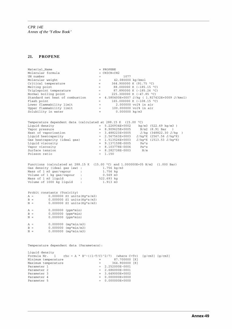
CPR 14EAnnex of the ‘Yellow Book’
Annex-49
21. PROPENE
Material_Name = PROPENEMolecular formula = CH3CH=CH2UN number = 1077Molecular weight = 42.080000 kg/kmolCritical temperature = 364.900000 K (91.75 °C)Melting point = 88.000000 K (-185.15 °C)Triplepoint temperature = 87.890000 K (-185.26 °C)Normal boiling point = 225.300000 K (-47.85 °C)Standard net heat of combustion = 4.580400E+0007 J/kg ( 1.927432E+0009 J/kmol)Flash point = 165.000000 K (-108.15 °C)Lower flammability limit = 2.000000 vol% in airUpper flammability limit = 100.000000 vol% in airSolubility in water = 0.000000 kg/m3
Temperature dependent data (calculated at 288.15 K (15.00 °C)Liquid density = 5.226934E+0002 kg/m3 (522.69 kg/m3 )Vapor pressure = 8.909625E+0005 N/m2 (8.91 Bar )Heat of vaporization = 3.488223E+0005 J/kg (348822.30 J/kg )Liquid heatcapacity = 2.567563E+0003 J/kg*K (2567.56 J/kg*K)Gas heatcapacity (ideal gas) = 1.513526E+0003 J/kg*K (1513.53 J/kg*K)Liquid viscosity = 9.137159E-0005 Pa*s Vapor viscosity = 8.103778E-0006 Pa*s Surface tension = 8.282738E-0003 N/m Poisson ratio = 1.150
Functions (calculated at 288.15 K (15.00 °C) and 1.000000E+05 N/m2 (1.000 Bar)Gas density (ideal gas law) : 1.756 kg/m3Mass of 1 m3 gas/vapour : 1.756 kgVolume of 1 kg gas/vapour : 0.569 m3Mass of 1 m3 liquid : 522.693 kgVolume of 1000 kg liquid : 1.913 m3
Probit constants (Toxicity)A = 0.000000 SI units(Kg*s/m3)B = 0.000000 SI units(Kg*s/m3)N = 0.000000 SI units(Kg*s/m3)
A = 0.000000 (ppm*min)B = 0.000000 (ppm*min)N = 0.000000 (ppm*min)
A = 0.000000 (mg*min/m3)B = 0.000000 (mg*min/m3)N = 0.000000 (mg*min/m3)
Temperature dependent data (Parameters):
Liquid densityFormula Nr. 1 rho = A * B^-((1-T/C)^2/7) (where C=Tc) [g/cm3] [g/cm3]Minimum temperature = 87.700000 [K]Maximum temperature = 364.900000 [K]Parameter 1 = 2.252000E-0001Parameter 2 = 2.686000E-0001Parameter 3 = 3.649000E+0002Parameter 4 = 0.000000E+0000Parameter 5 = 0.000000E+0000

Annex-50
Vapor pressureFormula Nr. 2 Log(P) = A + B/T + C*Log(T) + D*T + E*T^2 [mm Hg] [mm Hg]Minimum temperature = 123.000000 [K]Maximum temperature = 365.100000 [K]Parameter 1 = 3.687700E+0001Parameter 2 = -1.725500E+0003Parameter 3 = -1.205700E+0001Parameter 4 = 8.994800E-0003Parameter 5 = 0.000000E+0000
Heat of vaporizationFormula Nr. 3 Hv = A * ((C-T)/(C-B)^D (A=Hv1, B=T1, C=Tc) [cal/g] [cal/g]Minimum temperature = 87.700000 [K]Maximum temperature = 364.900000 [K]Parameter 1 = 1.046000E+0002Parameter 2 = 2.253000E+0002Parameter 3 = 3.649000E+0002Parameter 4 = 3.800000E-0001Parameter 5 = 0.000000E+0000
Liquid heatcapacityFormula Nr. 4 Cpl = A + B*T + C*T^2 + D*T^3 [cal/g/K] [cal/g/K]Minimum temperature = 87.700000 [K]Maximum temperature = 313.000000 [K]Parameter 1 = 4.706000E-0001Parameter 2 = 1.683000E-0003Parameter 3 = -1.682000E-0005Parameter 4 = 4.407000E-0008Parameter 5 = 0.000000E+0000
IG heatcapacityFormula Nr. 5 Cp = A + B*T + C*T^2 + D*T^3 [cal/mol] [cal/mol]Minimum temperature = 298.000000 [K]Maximum temperature = 1500.000000 [K]Parameter 1 = 6.800000E-0001Parameter 2 = 5.680000E-0002Parameter 3 = -2.860000E-0005Parameter 4 = 5.600000E-0009Parameter 5 = 0.000000E+0000
Liquid viscosityFormula Nr. 6 Log(Visc) = Ea + Eb/T + Ec*Log (T) + Ed*T + Ee*T*T (where Ec=0!) [centiPoise][centiPoise]Minimum temperature = 113.000000 [K]Maximum temperature = 364.900000 [K]Parameter 1 = -5.009000E+0000Parameter 2 = 4.132000E+0002Parameter 3 = 0.000000E+0000Parameter 4 = 1.771000E-0002Parameter 5 = -3.092000E-0005
Vapor viscosityFormula Nr. 7 Visc = A + B*T + C*T^2 [microPoise] [microPoise]Minimum temperature = 173.000000 [K]Maximum temperature = 1273.000000 [K]Parameter 1 = -5.601000E+0000Parameter 2 = 3.188000E-0001Parameter 3 = -6.291000E-0005Parameter 4 = 0.000000E+0000Parameter 5 = 0.000000E+0000
Surface TensionFormula Nr. 8 Sigma = A * ((C-T)/(C-B))^D (A=Sigma1, B=T1, C=Tc) [dynes/cm] [dynes/cm]Minimum temperature = 87.700000 [K]Maximum temperature = 364.900000 [K]Parameter 1 = 1.998000E+0001Parameter 2 = 2.030000E+0002Parameter 3 = 3.649000E+0002Parameter 4 = 1.179700E+0000Parameter 5 = 0.000000E+0000
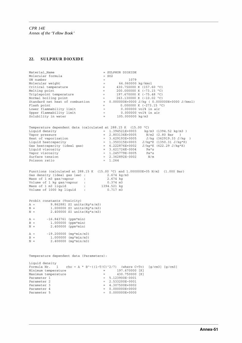
CPR 14EAnnex of the ‘Yellow Book’
Annex-51
22. SULPHUR DIOXIDE
Material_Name = SULPHUR DIOXIDEMolecular formula = SO2UN number = 1079Molecular weight = 64.060000 kg/kmolCritical temperature = 430.750000 K (157.60 °C)Melting point = 200.000000 K (-73.15 °C)Triplepoint temperature = 197.670000 K (-75.48 °C)Normal boiling point = 263.130000 K (-10.02 °C)Standard net heat of combustion = 0.000000E+0000 J/kg ( 0.000000E+0000 J/kmol)Flash point = 0.000000 K (-273.15 °C)Lower flammability limit = 0.000000 vol% in airUpper flammability limit = 0.000000 vol% in airSolubility in water = 105.000000 kg/m3
Temperature dependent data (calculated at 288.15 K (15.00 °C)Liquid density = 1.394521E+0003 kg/m3 (1394.52 kg/m3 )Vapor pressure = 2.803136E+0005 N/m2 (2.80 Bar )Heat of vaporization = 3.629193E+0005 J/kg (362919.33 J/kg )Liquid heatcapacity = 1.350315E+0003 J/kg*K (1350.31 J/kg*K)Gas heatcapacity (ideal gas) = 6.222876E+0002 J/kg*K (622.29 J/kg*K)Liquid viscosity = 3.621724E-0004 Pa*s Vapor viscosity = 1.245779E-0005 Pa*s Surface tension = 2.362892E-0002 N/m Poisson ratio = 1.264
Functions (calculated at 288.15 K (15.00 °C) and 1.000000E+05 N/m2 (1.000 Bar)Gas density (ideal gas law) : 2.674 kg/m3Mass of 1 m3 gas/vapour : 2.674 kgVolume of 1 kg gas/vapour : 0.374 m3Mass of 1 m3 liquid : 1394.521 kgVolume of 1000 kg liquid : 0.717 m3
Probit constants (Toxicity)A = 9.862881 SI units(Kg*s/m3)B = 1.000000 SI units(Kg*s/m3)N = 2.400000 SI units(Kg*s/m3)
A = -16.843761 (ppm*min)B = 1.000000 (ppm*min)N = 2.400000 (ppm*min)
A = -19.200000 (mg*min/m3)B = 1.000000 (mg*min/m3)N = 2.400000 (mg*min/m3)
Temperature dependent data (Parameters):
Liquid densityFormula Nr. 1 rho = A * B^-((1-T/C)^2/7) (where C=Tc) [g/cm3] [g/cm3]Minimum temperature = 197.670000 [K]Maximum temperature = 430.750000 [K]Parameter 1 = 5.123900E-0001Parameter 2 = 2.533200E-0001Parameter 3 = 4.307500E+0002Parameter 4 = 0.000000E+0000Parameter 5 = 0.000000E+0000

Annex-52
Vapor pressureFormula Nr. 2 Log(P) = A + B/T + C*Log(T) + D*T + E*T^2 [mm Hg] [mm Hg]Minimum temperature = 197.670000 [K]Maximum temperature = 430.750000 [K]Parameter 1 = 2.075270E+0001Parameter 2 = -1.831700E+0003Parameter 3 = -4.597200E+0000Parameter 4 = 6.785100E-0004Parameter 5 = 4.663200E-0007
Heat of vaporizationFormula Nr. 3 Hv = A * ((C-T)/(C-B)^D (A=Hv1, B=T1, C=Tc) [cal/g] [cal/g]Minimum temperature = 197.670000 [K]Maximum temperature = 430.750000 [K]Parameter 1 = 7.977000E+0001Parameter 2 = 3.142000E+0002Parameter 3 = 4.307500E+0002Parameter 4 = 4.128800E-0001Parameter 5 = 0.000000E+0000
Liquid heatcapacityFormula Nr. 4 Cpl = A + B*T + C*T^2 + D*T^3 [cal/g/K] [cal/g/K]Minimum temperature = 197.670000 [K]Maximum temperature = 263.130000 [K]Parameter 1 = 3.495600E-0001Parameter 2 = -1.321000E-0004Parameter 3 = 8.943900E-0008Parameter 4 = 8.704000E-0011Parameter 5 = 0.000000E+0000
IG heatcapacityFormula Nr. 5 Cp = A + B*T + C*T^2 + D*T^3 [cal/mol] [cal/mol]Minimum temperature = 100.000000 [K]Maximum temperature = 1500.000000 [K]Parameter 1 = 6.487700E+0000Parameter 2 = 1.258100E-0002Parameter 3 = -7.544000E-0006Parameter 4 = 1.528800E-0009Parameter 5 = 0.000000E+0000
Liquid viscosityFormula Nr. 6 Log(Visc) = Ea + Eb/T + Ec*Log (T) + Ed*T + Ee*T*T (where Ec=0!) [centiPoise][centiPoise]Minimum temperature = 239.650000 [K]Maximum temperature = 323.150000 [K]Parameter 1 = -8.538000E-0001Parameter 2 = 1.861800E+0002Parameter 3 = 0.000000E+0000Parameter 4 = -6.998000E-0004Parameter 5 = -3.825000E-0007
Vapor viscosityFormula Nr. 7 Visc = A + B*T + C*T^2 [microPoise] [microPoise]Minimum temperature = 200.000000 [K]Maximum temperature = 1000.000000 [K]Parameter 1 = -1.294600E+0001Parameter 2 = 5.104600E-0001Parameter 3 = -1.152000E-0004Parameter 4 = 0.000000E+0000Parameter 5 = 0.000000E+0000
Surface TensionFormula Nr. 8 Sigma = A * ((C-T)/(C-B))^D (A=Sigma1, B=T1, C=Tc) [dynes/cm] [dynes/cm]Minimum temperature = 197.670000 [K]Maximum temperature = 430.750000 [K]Parameter 1 = 1.862000E+0001Parameter 2 = 3.142000E+0002Parameter 3 = 4.307500E+0002Parameter 4 = 1.181000E+0000Parameter 5 = 0.000000E+0000

CPR 14EAnnex of the ‘Yellow Book’
Annex-53
23. TOLUENE
Material_Name = TOLUENEMolecular formula = C6H5CH3UN number = 1294Molecular weight = 92.100000 kg/kmolCritical temperature = 591.800000 K (318.65 °C)Melting point = 178.000000 K (-95.15 °C)Triplepoint temperature = 178.180000 K (-94.97 °C)Normal boiling point = 383.600000 K (110.45 °C)Standard net heat of combustion = 4.055000E+0007 J/kg ( 3.734655E+0009 J/kmol)Flash point = 277.000000 K (3.85 °C)Lower flammability limit = 1.270000 vol% in airUpper flammability limit = 100.000000 vol% in airSolubility in water = 0.500000 kg/m3
Temperature dependent data (calculated at 288.15 K (15.00 °C)Liquid density = 8.710100E+0002 kg/m3 (871.01 kg/m3 )Vapor pressure = 2.196688E+0003 N/m2 (0.02 Bar )Heat of vaporization = 4.159887E+0005 J/kg (415988.71 J/kg )Liquid heatcapacity = 1.666549E+0003 J/kg*K (1666.55 J/kg*K)Gas heatcapacity (ideal gas) = 1.124195E+0003 J/kg*K (1124.20 J/kg*K)Liquid viscosity = 6.275112E-0004 Pa*s Vapor viscosity = 6.636030E-0006 Pa*s Surface tension = 2.909345E-0002 N/m Poisson ratio = 1.087
Functions (calculated at 288.15 K (15.00 °C) and 1.000000E+05 N/m2 (1.000 Bar)Gas density (ideal gas law) : 3.844 kg/m3Mass of 1 m3 gas/vapour : 3.844 kgVolume of 1 kg gas/vapour : 0.260 m3Mass of 1 m3 liquid : 871.010 kgVolume of 1000 kg liquid : 1.148 m3
Probit constants (Toxicity)A = 0.000000 SI units(Kg*s/m3)B = 0.000000 SI units(Kg*s/m3)N = 0.000000 SI units(Kg*s/m3)
A = 0.000000 (ppm*min)B = 0.000000 (ppm*min)N = 0.000000 (ppm*min)
A = 0.000000 (mg*min/m3)B = 0.000000 (mg*min/m3)N = 0.000000 (mg*min/m3)
Temperature dependent data (Parameters):
Liquid densityFormula Nr. 1 rho = A * B^-((1-T/C)^2/7) (where C=Tc) [g/cm3] [g/cm3]Minimum temperature = 178.000000 [K]Maximum temperature = 591.800000 [K]Parameter 1 = 2.883000E-0001Parameter 2 = 2.624000E-0001Parameter 3 = 5.918000E+0002Parameter 4 = 0.000000E+0000Parameter 5 = 0.000000E+0000

Annex-54
Vapor pressureFormula Nr. 2 Log(P) = A + B/T + C*Log(T) + D*T + E*T^2 [mm Hg] [mm Hg]Minimum temperature = 213.000000 [K]Maximum temperature = 593.600000 [K]Parameter 1 = 1.152100E+0002Parameter 2 = -4.918100E+0003Parameter 3 = -4.346700E+0001Parameter 4 = 3.854800E-0002Parameter 5 = -1.349600E-0005
Heat of vaporizationFormula Nr. 3 Hv = A * ((C-T)/(C-B)^D (A=Hv1, B=T1, C=Tc) [cal/g] [cal/g]Minimum temperature = 178.000000 [K]Maximum temperature = 591.800000 [K]Parameter 1 = 8.610000E+0001Parameter 2 = 3.836000E+0002Parameter 3 = 5.918000E+0002Parameter 4 = 3.800000E-0001Parameter 5 = 0.000000E+0000
Liquid heatcapacityFormula Nr. 4 Cpl = A + B*T + C*T^2 + D*T^3 [cal/g/K] [cal/g/K]Minimum temperature = 178.000000 [K]Maximum temperature = 583.000000 [K]Parameter 1 = -1.461000E-0001Parameter 2 = 4.584000E-0003Parameter 3 = -1.346000E-0005Parameter 4 = 1.425000E-0008Parameter 5 = 0.000000E+0000
IG heatcapacityFormula Nr. 5 Cp = A + B*T + C*T^2 + D*T^3 [cal/mol] [cal/mol]Minimum temperature = 298.000000 [K]Maximum temperature = 1500.000000 [K]Parameter 1 = -9.340000E+0000Parameter 2 = 1.385000E-0001Parameter 3 = -8.720000E-0005Parameter 4 = 2.060000E-0008Parameter 5 = 0.000000E+0000
Liquid viscosityFormula Nr. 6 Log(Visc) = Ea + Eb/T + Ec*Log (T) + Ed*T + Ee*T*T (where Ec=0!) [centiPoise][centiPoise]Minimum temperature = 233.000000 [K]Maximum temperature = 591.800000 [K]Parameter 1 = -2.553000E+0000Parameter 2 = 5.591000E+0002Parameter 3 = 0.000000E+0000Parameter 4 = 1.987000E-0003Parameter 5 = -1.954000E-0006
Vapor viscosityFormula Nr. 7 Visc = A + B*T + C*T^2 [microPoise] [microPoise]Minimum temperature = 273.000000 [K]Maximum temperature = 1273.000000 [K]Parameter 1 = -8.421000E+0000Parameter 2 = 2.711000E-0001Parameter 3 = -4.018000E-0005Parameter 4 = 0.000000E+0000Parameter 5 = 0.000000E+0000
Surface TensionFormula Nr. 8 Sigma = A * ((C-T)/(C-B))^D (A=Sigma1, B=T1, C=Tc) [dynes/cm] [dynes/cm]Minimum temperature = 178.000000 [K]Maximum temperature = 591.800000 [K]Parameter 1 = 2.852000E+0001Parameter 2 = 2.930000E+0002Parameter 3 = 5.918000E+0002Parameter 4 = 1.236400E+0000Parameter 5 = 0.000000E+0000
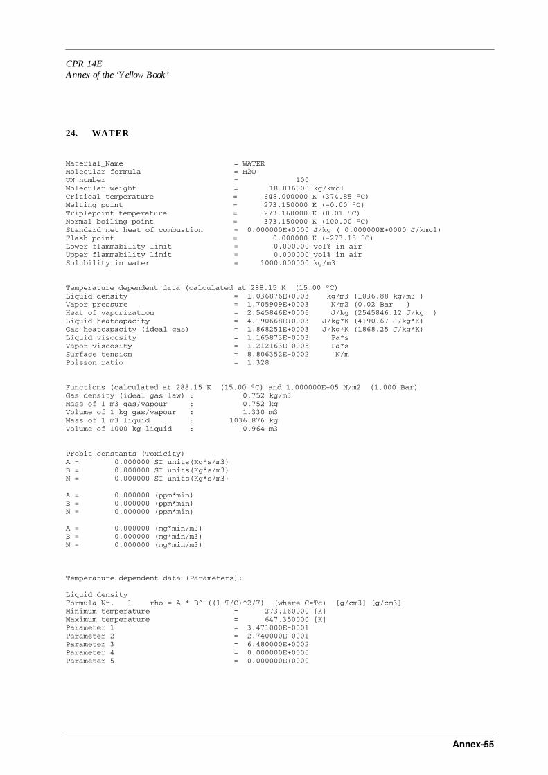
CPR 14EAnnex of the ‘Yellow Book’
Annex-55
24. WATER
Material_Name = WATERMolecular formula = H2OUN number = 100Molecular weight = 18.016000 kg/kmolCritical temperature = 648.000000 K (374.85 °C)Melting point = 273.150000 K (-0.00 °C)Triplepoint temperature = 273.160000 K (0.01 °C)Normal boiling point = 373.150000 K (100.00 °C)Standard net heat of combustion = 0.000000E+0000 J/kg ( 0.000000E+0000 J/kmol)Flash point = 0.000000 K (-273.15 °C)Lower flammability limit = 0.000000 vol% in airUpper flammability limit = 0.000000 vol% in airSolubility in water = 1000.000000 kg/m3
Temperature dependent data (calculated at 288.15 K (15.00 °C)Liquid density = 1.036876E+0003 kg/m3 (1036.88 kg/m3 )Vapor pressure = 1.705909E+0003 N/m2 (0.02 Bar )Heat of vaporization = 2.545846E+0006 J/kg (2545846.12 J/kg )Liquid heatcapacity = 4.190668E+0003 J/kg*K (4190.67 J/kg*K)Gas heatcapacity (ideal gas) = 1.868251E+0003 J/kg*K (1868.25 J/kg*K)Liquid viscosity = 1.165873E-0003 Pa*s Vapor viscosity = 1.212163E-0005 Pa*s Surface tension = 8.806352E-0002 N/m Poisson ratio = 1.328
Functions (calculated at 288.15 K (15.00 °C) and 1.000000E+05 N/m2 (1.000 Bar)Gas density (ideal gas law) : 0.752 kg/m3Mass of 1 m3 gas/vapour : 0.752 kgVolume of 1 kg gas/vapour : 1.330 m3Mass of 1 m3 liquid : 1036.876 kgVolume of 1000 kg liquid : 0.964 m3
Probit constants (Toxicity)A = 0.000000 SI units(Kg*s/m3)B = 0.000000 SI units(Kg*s/m3)N = 0.000000 SI units(Kg*s/m3)
A = 0.000000 (ppm*min)B = 0.000000 (ppm*min)N = 0.000000 (ppm*min)
A = 0.000000 (mg*min/m3)B = 0.000000 (mg*min/m3)N = 0.000000 (mg*min/m3)
Temperature dependent data (Parameters):
Liquid densityFormula Nr. 1 rho = A * B^-((1-T/C)^2/7) (where C=Tc) [g/cm3] [g/cm3]Minimum temperature = 273.160000 [K]Maximum temperature = 647.350000 [K]Parameter 1 = 3.471000E-0001Parameter 2 = 2.740000E-0001Parameter 3 = 6.480000E+0002Parameter 4 = 0.000000E+0000Parameter 5 = 0.000000E+0000

Annex-56
Vapor pressureFormula Nr. 2 Log(P) = A + B/T + C*Log(T) + D*T + E*T^2 [mm Hg] [mm Hg]Minimum temperature = 273.160000 [K]Maximum temperature = 647.130000 [K]Parameter 1 = 2.988850E+0001Parameter 2 = -3.152900E+0003Parameter 3 = -7.315200E+0000Parameter 4 = 1.126200E-0005Parameter 5 = 1.804800E-0006
Heat of vaporizationFormula Nr. 3 Hv = A * ((C-T)/(C-B)^D (A=Hv1, B=T1, C=Tc) [cal/g] [cal/g]Minimum temperature = 273.160000 [K]Maximum temperature = 647.130000 [K]Parameter 1 = 4.759000E+0002Parameter 2 = 4.601000E+0002Parameter 3 = 6.480000E+0002Parameter 4 = 3.774600E-0001Parameter 5 = 0.000000E+0000
Liquid heatcapacityFormula Nr. 4 Cpl = A + B*T + C*T^2 + D*T^3 [cal/g/K] [cal/g/K]Minimum temperature = 273.150000 [K]Maximum temperature = 533.150000 [K]Parameter 1 = 6.933800E-0001Parameter 2 = 3.194400E-0003Parameter 3 = -1.101000E-0005Parameter 4 = 1.259900E-0008Parameter 5 = 0.000000E+0000
IG heatcapacityFormula Nr. 5 Cp = A + B*T + C*T^2 + D*T^3 [cal/mol] [cal/mol]Minimum temperature = 100.000000 [K]Maximum temperature = 1500.000000 [K]Parameter 1 = 7.981000E+0000Parameter 2 = -9.050000E-0004Parameter 3 = 4.294100E-0006Parameter 4 = -1.507000E-0009Parameter 5 = 0.000000E+0000
Liquid viscosityFormula Nr. 6 Log(Visc) = Ea + Eb/T + Ec*Log (T) + Ed*T + Ee*T*T (where Ec=0!) [centiPoise][centiPoise]Minimum temperature = 273.150000 [K]Maximum temperature = 643.150000 [K]Parameter 1 = -8.426800E+0000Parameter 2 = 1.559300E+0003Parameter 3 = 0.000000E+0000Parameter 4 = 1.334000E-0002Parameter 5 = -9.176000E-0006
Vapor viscosityFormula Nr. 7 Visc = A + B*T + C*T^2 [microPoise] [microPoise]Minimum temperature = 373.150000 [K]Maximum temperature = 1073.100000 [K]Parameter 1 = -3.536800E+0001Parameter 2 = 4.243600E-0001Parameter 3 = -1.268000E-0005Parameter 4 = 0.000000E+0000Parameter 5 = 0.000000E+0000
Surface TensionFormula Nr. 8 Sigma = A * ((C-T)/(C-B))^D (A=Sigma1, B=T1, C=Tc) [dynes/cm] [dynes/cm]Minimum temperature = 273.160000 [K]Maximum temperature = 647.130000 [K]Parameter 1 = 4.054000E+0001Parameter 2 = 4.601000E+0002Parameter 3 = 6.480000E+0002Parameter 4 = 1.193900E+0000Parameter 5 = 0.000000E+0000