methods for lidar point cloud classification using local

Methods for LiDAR point cloud classification using localneighborhood statistics

Angela M. Kim, Richard C. Olsen, Fred A. Kruse

Naval Postgraduate School, Remote Sensing Center and Physics Department,833 Dyer Road, Monterey, CA, USA

ABSTRACT

LiDAR data are available in a variety of publicly-accessible forums, providing high-resolution, accurate 3-dimensional information about objects at the Earth’s surface. Automatic extraction of information from LiDARpoint clouds, however, remains a challenging problem. The focus of this research is to develop methods forpoint cloud classification and object detection which can be customized for specific applications. The methodspresented rely on analysis of statistics of local neighborhoods of LiDAR points. A multi-dimensional vectorcomposed of these statistics can be classified using traditional data classification routines. Local neighborhoodstatistics are defined, and examples are given of the methods for specific applications such as building extrac-tion and vegetation classification. Results indicate the feasibility of the local neighborhood statistics approachand provide a framework for the design of customized classification or object detection routines for LiDARpoint clouds.

Keywords: LiDAR, point cloud, classification, statistics, local neighborhood

1. INTRODUCTION

It is clear from a visual inspection of LiDAR point cloud data that the 3-dimensional arrangement of LiDARpoints is useful for distinguishing materials and objects in a scene. Characteristics of the distribution of pointssuch as smoothness, regularity, and vertical scatter may help determine what type of surface or object the pointsrepresent. In this work, local neighborhoods of LiDAR points were examined and a series of statistics weredefined to quantify these characteristics. Methods for defining local neighborhoods are discussed in Section 4,and a selection of local neighborhood statistics is discussed in Section 5.

The statistical attributes were combined into feature vectors that were then used to segment the pointcloud data into classes using traditional data classification routines. Not all attributes were useful for each sceneclassification task. The utility of individual statistical measures depends upon the characteristics of the particularLiDAR point cloud being examined, and the goal of the classification scheme. To determine which features weremost useful for creating separable classes, the histograms of values for each statistic within a training regionof interest were examined. Features that maximize the separability of classes were chosen for inclusion in theclassification routine (Section 6).

Two methods for classifying the LiDAR feature vectors, one supervised and one unsupervised, are discussedin Section 7. Results using both classification approaches and different combinations of statistical features arecompared in Section 8. A summary of results and directions for future work are given in the final two sections(Sections 9 and 10).

Further author information:A.M.K.: E-mail: [email protected], Telephone: 1 401 647 3536

Laser Radar Technology and Applications XVIII, edited by Monte D. Turner, Gary W. Kamerman, Proc. of SPIE Vol. 8731, 873103 · © 2013 SPIE · CCC code: 0277-786X/13/$18 · doi: 10.1117/12.2015709

Proc. of SPIE Vol. 8731 873103-1

Downloaded From: http://proceedings.spiedigitallibrary.org/ on 05/27/2017 Terms of Use: http://spiedigitallibrary.org/ss/termsofuse.aspx

2. PREVIOUS WORK

Chehata et al. (2009) present a variety of statistics-based point cloud features and perform feature selection fromLiDAR data using a random forests classification.1 The ISPRS Commission III, Working Group 4, on 3D sceneanalysis provided a benchmark dataset for comparing methods of urban object classification and 3D buildingreconstruction. An accompanying report summarizes the success of the participants in classifying buildings andtrees.2 Using the benchmark dataset, Niemeyer et al. (2012) used an approach similar to Chehata et. al (2009),incorporating point cloud statistics, but instead made use of a conditional random field classification scheme toincorporate contextual information.1,3

Brodu and Lague (2012) present a multi-scale dimensionality approach for classifying terrestrial laser scanningdata.4 The method relies on calculating the principal components of the matrix of xyz-coordinates of localneighborhoods of points. By analyzing the percentage of variance explained by each principal component, thelocal neighborhood of points can be classified as being linear, planar, or globular. Looking at the dimensionalityover varying spatial scales allows points to be classified.

The approach for classifying LiDAR point cloud data using point cloud statistics based features presented inthis paper is a very similar approach to that presented in Chehata et. al (2009) or Niemeyer et. al (2012).1,3 Weuse slightly different statistics, however, apply the multi-scale approach of Brodu and Lague (2012) to additionalstatistics, and use different methods for feature selection and classification.4

3. THE STUDY AREA AND LIDAR DATASET

LiDAR data were acquired for selected areas of California during 2010 by the Association of Monterey Bay AreaGovernments (AMBAG), via a USGS grant through the American Reinvestment and Recovery Act of 2009. Theprimary dataset used for this paper was collected for a portion of Camp Roberts (near Paso Robles, California)over multiple days in September, 2010, with a point density of ∼2.5 points per square meter. Bare-earth DigitalElevation Models (DEMs) with a resolution of 3-meter pixels were delivered with the data.

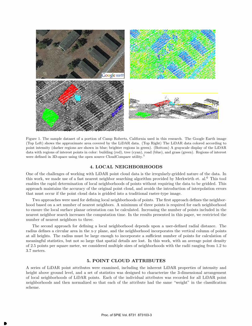
Regions of interest were selected in 3D-space using the open source CloudCompare utility developed by DanielGirardeau-Montaut.5 This tool enables selection of “tree” points, while excluding LiDAR returns from groundunderneath the tree. Similarly, the “building” ROI only contains rooftop points. Returns that may have comefrom the side of the building were excluded (Figure 1).



At-:k

".ª

, /%,/

ª/; .4

Figure 1. The sample dataset of a portion of Camp Roberts, California used in this research. The Google Earth image(Top Left) shows the approximate area covered by the LiDAR data. (Top Right) The LiDAR data colored according topoint intensity (darker regions are shown in blue; brighter regions in green). (Bottom) A grayscale display of the LiDARdata with regions of interest points in color: building (red), tree (cyan), road (blue), and grass (green). Regions of interestwere defined in 3D-space using the open source CloudCompare utility.5

4. LOCAL NEIGHBORHOODS

One of the challenges of working with LiDAR point cloud data is the irregularly-gridded nature of the data. Inthis work, we made use of a fast nearest neighbor searching algorithm provided by Merkwirth et. al.6 This toolenables the rapid determination of local neighborhoods of points without requiring the data to be gridded. Thisapproach maintains the accuracy of the original point cloud, and avoids the introduction of interpolation errorsthat must occur if the point cloud data is gridded into a traditional raster-type image.

Two approaches were used for defining local neighborhoods of points. The first approach defines the neighbor-hood based on a set number of nearest neighbors. A minimum of three points is required for each neighborhoodto ensure the local surface planar orientation can be calculated. Increasing the number of points included in thenearest neighbor search increases the computation time. In the results presented in this paper, we restricted thenumber of nearest neighbors to three.

The second approach for defining a local neighborhood depends upon a user-defined radial distance. Theradius defines a circular area in the x-y plane, and the neighborhood incorporates the vertical column of pointsat all heights. The radius must be large enough to incorporate a sufficient number of points for calculation ofmeaningful statistics, but not so large that spatial details are lost. In this work, with an average point densityof 2.5 points per square meter, we considered multiple sizes of neighborhoods with the radii ranging from 1.2 to3.7 meters.

5. POINT CLOUD ATTRIBUTES

A series of LiDAR point attributes were examined, including the inherent LiDAR properties of intensity andheight above ground level, and a set of statistics was designed to characterize the 3-dimensional arrangementof local neighborhoods of LiDAR points. Each of the individual attributes was recorded for all LiDAR pointneighborhoods and then normalized so that each of the attribute had the same “weight” in the classificationscheme.



5.1 Height Above Ground Level and Intensity

It is straightforward to make use of the height above ground level and return intensity values to classify LiDARpoint cloud data. While the return intensity values are not typically normalized between flight lines, the relativeintensity of points may be useful in distinguishing different materials.

A DEM or some other estimate of the bare earth surface is required to determine a point’s height aboveground level. In this work, we made use of the 3-meter resolution DEMs that were delivered by the vendor. Thefast nearest neighbor searching algorithm of Merkwirth et. al. was used to determine nearest DEM pixels toeach LiDAR point.6 The elevation of the nearest DEM pixel was subtracted from the elevation of the LiDARpoint to determine the height above ground level of each point.

5.2 Differences of Elevations

This statistic captures the average differences in elevations of neighborhoods of points. The statistic is calculatedby subtracting the minimum elevation within the neighborhood from the mean of elevations of all points withina neighborhood.

5.3 Standard Deviations of Elevations

This statistic is a useful measure of “smoothness”. This statistic is simply the standard deviation of elevationsof all points within a neighborhood.

5.4 Standard Deviations of Intensity Values

This statistic gives a measure of visual texture, and is calculated by finding the standard deviation of intensityvalues of all points within a neighborhood.

5.5 Angle of Planar Surface Normal

In this paper, this statistic was only calculated for neighborhoods defined using a point’s three nearest neighbors.The three nearest neighbors of each LiDAR point were used to define a plane. The deviation of the surface normalof the plane from vertical is recorded.

5.6 Principal Component Percentage of Variance

This statistic is adapted from Brodu and Lague (2012).4 For each neighborhood of points, the principal com-ponents of the matrix of xyz-coordinates is calculated. The percentage of the total variance explained by eachprincipal component gives an indication of the “dimensionality” of the object. For example, to explain the loca-tion of a point on a linear object (such as a telephone wire), only a single measurement is needed. The distance inthe direction of the axis aligned with the telephone wire is sufficient for defining the point’s location. Therefore,a set of points representing a linear feature will have most of the variance in its xyz-coordinates explained bythe first principal component. A planar surface, where points are spread in two dimensions, will require twocomponents to define the location of points. The first two principal components will be necessary for explainingmost of the variance in the data. Finally, if all three principal components are needed to represent a significantpercentage of the variance, the object is 3-dimensional. Figures 2 and 3 show an example point cloud created todemonstrate this concept.

The dimensionality of an object also depends upon the spatial scale at which it is examined. An object thatlooks planar close up (at a small spatial scale) may be 3-dimensional at a larger spatial scale. Further, thismulti-scale behavior will vary for different materials. Calculating this statistic at multiple spatial scales is usefulfor distinguishing different types of materials.

5.7 Point Density

The point density is determined by dividing the total number of points in a neighborhood by the square of theneighborhood radius.



Perspective Views of Sample Point Cloud with Linear, Planar, and 3D Features

1D Linear Feature2D Planar Feature3D Feature

-50

100

50

o

-50

15-

10-

5-

N 0-

-5-

-10-

-1560

-20100

50

-50 -100 50X

Y -100-100 -50 50 100

._'.'Z:

: ;.F1t .

k 1=

. '

40 20 0 -20 -40 -60

100

7, 80

ÉFc 8 60d q60 0aS 1...

ÿÿ40d

a.20

o

Percentage of Variance Explained by Each Principal Component

1

1D Linear Feature

e 2D Planar Feature

° 3D Feature

2Principal Component Number

3

Variability of Feature Vectorslr

f-0.8

', 0.6

0.4 _ GrasBuil

g 0.2 Mi Boad .7i Treez o `D 9 A h 0 4 6 0 10 15- 1 19 1A 1h 1 ti4 4' 10 ry0

I I II I

tig h4' ti 4'## 9h 9\ # #Attribute

Figure 2. An example point cloud with linear (red), planar (green), and 3D objects (blue).

Figure 3. The percentage of variance explained by each principal component for a linear (red), planar (green), and 3Dobject (blue). The linear feature requires only one principal component to explain all of the variance in the xyz-coordinates.

6. FEATURE SELECTION

Many of the features described in Section 5 are similar for multiple classes of materials. In Figure 4, the shadedregions represent the variability in the feature vectors for each of the four regions of interest. This figure illustratesthat the intraclass variability often exceeds the differences between classes. It is therefore necessary to choose asubset of features that maximize the class separability.

Figure 4. The mean feature vectors for each region of interest, with the variability of each class represented by the shadedregion. The intraclass variability of the features often exceeds the differences between classes.



The features as plotted in Figure 4 are as follows:

1. Differences of elevations (1.2-m neighborhood)



4. Differences of elevations (3-m neighborhood)


6. Differences of elevations (3-nearest neighbors)

7. Standard deviation of elevations (1.2-m)



10. Standard deviation of elevations (3-m)


12. Standard deviation of elevations (3-nearest neigh-bors)

13. Standard deviation of intensities (1.2-m)



16. Standard deviation of intensities (3-m)


18. Standard deviation of intensities (3-nearest neigh-bors)

19. Angle (3-nearest neighbors)

20. Percentage of variance - 1st Principal Component(PC) (1.2-m)

21. Percentage of variance - 1st PC (1.8-m)


23. Percentage of variance - 1st PC (3-m)


25. Percentage of variance - 2nd PC (1.2-m)



28. Percentage of variance - 2nd PC (3-m)


30. Percentage of variance - 3rd PC (1.2-m)



33. Percentage of variance - 3rd PC (3-m)


35. Point density (1.2-m)



38. Point density (3-m)


40. Height above ground level

41. Intensity

To select the most useful features for scene classification, the average distance between class means and theaverage standard deviation of values were measured for each attribute. The most useful attributes were chosenas those for which the average distance between class means exceeds the average standard deviation. For thesample dataset used in this paper, the attributes meeting this criterium are the following:

• 4 and 5: Differences of elevations (3-m and 3.7-m radius neighborhoods)

• 9 - 11: Standard deviation of elevations (2.4, 3, and 3.7-m radius neighborhoods)

• 16 - 18: Standard deviation of intensity values (3 and 3.7-m radius neighborhoods and 3-nearest neighborsneighborhood)

• 37 - 39: Point density (2.4, 3, 3.7-m radius neighborhoods)

• 41: Intensity

Although in this case the point density features meet the criteria for being useful for separating the classes,it is unlikely that these features would be useful for scene classification, as the point density has more to do withcollection geometry than any characteristic of the materials in the scene. A second subset of features was chosenusing all of the separable features except for the point density features (statistics 4, 5, 9-11, 16-18 and 41). Athird subset of features was defined subjectively by choosing features that appear to have distinct class means(statistics 4, 5, 8-11, 13, 15-18, 22, 25, 31, 32 and 41). Classification results using these subsets are compared toresults of classification based on only the height above ground level and intensity information, and classificationusing all available features in Section 7.



s;

...17.%

7. CLASSIFICATION METHODS

Statistics of local neighborhoods were used to define a series of attributes for each LiDAR point. These attributescomprise a feature vector for each LiDAR point. The feature vectors were classified using traditional dataprocessing techniques.7 Both a supervised “Spectral Angle Mapper (SAM)” and an unsupervised “KMEANS”classification method were considered here.

For the supervised SAM classification technique, training regions of interest (as shown in Figure 1) are used todesign classification decision criteria. The SAM classifier assigns feature vectors to a class based on minimizingthe angle between the feature vector and the mean feature vector of the training class.8 The angle betweenvectors is calculated using the well known formula:

Angle = arccos

(A ·B||A|| ||B||

)(1)

A minimum angle threshold can be defined so that points that are not close to any of the training classesremain unclassified. A threshold of 0.05 radians was used for the work presented in this paper.

For the unsupervised KMEANS classification method, the user must define the number of clusters to be used.Four clusters were used for this paper. The KMEANS algorithm randomly chooses cluster centers, and thenassigns vectors to the nearest cluster center. The cluster centers are then updated, and the process is repeateduntil cluster centers stabilize, or a certain number of iterations have been completed. Because the initial clustercenters are randomly assigned, running the classifier more than once may produce different results.9

8. COMPARISON OF RESULTS

The KMEANS classifier is an unsupervised routine, with classes being randomly assigned. In the figures showingKMEANS classification results below, the colors do not necessarily correspond to particular classes, althoughsome effort was made to match the KMEANS class colors to the SAM classes for purposes of visual comparison.For the SAM classifier, class colors correspond to the regions of interest as shown in Figure 1. Unclassified pointsare shown in black.

8.1 Classification Using Height Above Ground Level and Intensity

It is a fairly standard practice to classify LiDAR data using the height above ground level and intensity infor-mation. Results of a supervised SAM classification and an unsupervised KMEANS classification are shown inFigure 5. The SAM classification results are very poor. The KMEANS method does a slightly better job ofdistinguishing the road from the dry grass covered ground, but trees and buildings are confused.

Figure 5. Spectral angle mapper (SAM) supervised classification results (L) and KMEANS unsupervised classificationresults (R) using only height above ground level and return intensity information.



%S

:z1;4111:4". jJ

C

L.r,`.?

v° } :+id°

' ?:' ,i';.`.i :sn

'.iM

''+357' ..-t;. S

A-;ïitaS

.`Ì .P'

0. A

st

4. a.4tS,%-

(,

14'

vte'.- %tor

SV

8.2 Classification Using All Available Attributes

Results of the classification using all of the available LiDAR point attributes - statistical measures based onneighborhoods of points, along with the height above ground level and intensity information - are shown inFigure 6. In this case, the SAM and KMEANS classifier produce similar results, with a slightly cleaner resultfrom the SAM classifier. For both classification methods, there is some confusion in the grass and road classes.Also, while buildings are mostly classified correctly, the edges of the buildings are confused with the tree class.

Figure 6. Spectral angle mapper (SAM) supervised classification results (L) and KMEANS unsupervised classificationresults (R) using all available local neighborhood statistics, height above ground level, and return intensity information.

8.3 Classification Using Selected Subsets of Attributes

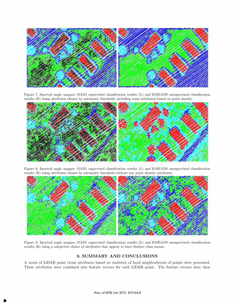
It is more efficient, and with an appropriate selection - more accurate, to use a subset of attributes. As discussedin Section 6, an automated method of choosing a feature subset is to select those attributes for which the averagedistance between class means is greater than the average standard deviation of the class. Using this automatedattribute selection method, twelve features were selected (4, 5, 9-11, 16-18, and 37-40). These features includeattributes based on the differences in elevations, the standard deviation of elevations, standard deviation ofintensity values, point density, and height above ground level. Results of classification using this subset ofattributes are shown in Figure 7.

While the point density attributes meet the criteria for the automated feature selection, they are not expectedto be useful for scene classification in general, since the point density is dependent upon sensor collection geometrymore than on any material characteristics. By comparing classification results incorporating the point densityfeatures (Figure 7), and classification results excluding these features (Figure 8), we can see that for this sampledataset, inclusion of the point density attributes improved the distinction of buildings and trees, but causedconfusion among the road and grass classes.

The automated method used for feature selection in this paper is very simple and not overly successful.A subjective choice of a subset of attributes that appear to have distinct class means produced better results(Figure 9). The subset includes statistics 4, 5, 8-11, 13, 15-18, 22, 25, 31, 32, and 41. These features includeattributes based on differences in elevations, standard deviation of elevations, standard deviation of intensities,return intensity, and some of the principal component based features. In this case, the SAM routine successfullydistinguished the four classes. Some confusion remained along the edges of buildings, with these points beingincorrectly classified as belonging to the tree class. The KMEANS routine was also successful in distinguishingbuildings from trees, but did a much poorer job of separating the road and grass classes.



;P.

. r,gemdds,..4,0,

ry; .

ß1 ?5

40'4 0:,4111

o".

i

Ktl

+4*

V-V

cre.

..44.1

.1"..eV

.1/4...

'

Figure 7. Spectral angle mapper (SAM) supervised classification results (L) and KMEANS unsupervised classificationresults (R) using attributes chosen by automatic threshold, including some attributes based on point density.

Figure 8. Spectral angle mapper (SAM) supervised classification results (L) and KMEANS unsupervised classificationresults (R) using attributes chosen by automatic threshold without any point density attributes.

Figure 9. Spectral angle mapper (SAM) supervised classification results (L) and KMEANS unsupervised classificationresults (R) using a subjective choice of attributes that appear to have distinct class means.

9. SUMMARY AND CONCLUSIONS

A series of LiDAR point cloud attributes based on statistics of local neighborhoods of points were presented.These attributes were combined into feature vectors for each LiDAR point. The feature vectors were then



classified using traditional image processing techniques, including a supervised spectral angle mapper (SAM)classification and an unsupervised KMEANS classification.

A simple method was presented for automated feature selection based on finding features that have an averagedistance between class means greater than the average standard deviation of the classes. This simple method offeature selection does not lead to a very successful classification result. A subjectively chosen subset of featuresbased on choosing features that appear to have distinct class means was found to provide the best classificationresult.

Results indicate that inclusion of the local neighborhood statistical attributes leads to an improved discrim-ination of materials over a classification using only height above ground level and intensity information.

10. FUTURE WORK

The methods presented here are sensitive to local neighborhood size. The best method for choosing an appropriateneighborhood size is an ongoing area of research. It is dependent upon the size of the features to be distinguished,the density of the LiDAR point cloud, and the desired speed of processing.

Feature selection affects the efficiency of processing and the accuracy of the classification result. Subjectivelychoosing the features which had the most distinct training class means worked well in this case, but an automatedmethod for feature selection would be preferable.

Application of the methods presented here to a dataset with ground truth, such as the benchmark datasetprovided by the ISPRS Commission III, Working Group 4, will allow for a quantitative assessment of the method.2

REFERENCES

[1] Chehata, N., Guo, L., and Mallet, C., “Airborne LiDAR feature selection for urban classification usingrandom forests,” Laser Scanning 2009, IAPRS 38(Part 3/W8), 207–212 (2009).

[2] Rottensteiner, F., Sohn, G., Jung, J., Gerke, M., Baillard, C., Benitez, S., and Breitkopf, U.,“The ISPRS benchmark on urban object classification and 3D building reconstruction,” ISPRS Commis-sion III, WGIII/4 , 1–6 (2012).

[3] Niemeyer, J., Rottensteiner, F., and Soergel, U., “Conditional random fields for LiDAR point cloud classifi-cation in complex urban areas,” ISPRS Annals of Photogrammetry, Remote Sensing and Spatial InformationSciences I-3, 263–268 (2012).

[4] Brodu, N. and Lague, D., “3D terrestrial lidar data classification of complex natural scenes using a multi-scaledimensionality criterion: Applications in geomorphology,” ISPRS Journal of Photogrammetry and RemoteSensing 68(C), 121–134 (2012).

[5] Girardeau-Montaut, D., “CloudCompare Open Source Project,” http://www.danielgm.net/cc/ .

[6] Merkwirth, C., Parlitz, U., Wedekind, I., Engster, D., and Lauterborn, W., “OpenTSTOOL User Manual,”www.physik3.gwdg.de/tstool/ .

[7] Richards, J. A. and Jia, X., [Remote Sensing Digital Image Analysis–An Introduction ], Springer, 4 ed. (2006).

[8] Kruse, F. A., Lefkoff, A. B., Boardman, J. B., Shapiro, A. T., Barloon, P. J., and Goetz, A. F. H., “TheSpectral Image Processing System (SIPS) – Interactive Visualization and Analysis of Imaging SpectrometerData,” Remote Sensing of Environment 44, 144–163 (1993).

[9] Seber, G. A. F., [Multivariate Observations ], John Wiley & Sons, Inc. (1984).

Proc. of SPIE Vol. 8731 873103-10


methods for lidar point cloud classification using local

Documents