methods for the analysis of short-term variability of …3 korhonen, ilkka. methods for the analysis...
TRANSCRIPT

VTT PUBLICATIONS 316
TECHNICAL RESEARCH CENTRE OF FINLANDESPOO 1997
Methods for the analysis ofshort-term variability of heart rateand blood pressure in frequency
domain
Ilkka Korhonen
VTT Information Technology
Thesis for the degree of Doctor of Technology to be presented with duepermission for public examination and criticism in Auditorium HB116,
Hermitec at Tampere University of Technology, on the 12th of September 1997,at 12 o’clock noon.

ISBN 951–38–5066–8 (soft back edition)ISSN 1235–0621 (soft back edition)
ISBN 951–38–5067–6 (URL: http://www.inf.vtt.fi/pdf/)ISSN 1455–0849 (URL: http://www.inf.vtt.fi/pdf/)
Copyright © Valtion teknillinen tutkimuskeskus (VTT) 1997
JULKAISIJA – UTGIVARE – PUBLISHER
Valtion teknillinen tutkimuskeskus (VTT), Vuorimiehentie 5, PL 2000, 02044 VTTpuh. vaihde (09) 4561, faksi (09) 456 4374
Statens tekniska forskningscentral (VTT), Bergsmansvägen 5, PB 2000, 02044 VTTtel. växel (09) 4561, fax (09) 456 4374
Technical Research Centre of Finland (VTT), Vuorimiehentie 5, P.O.Box 2000, FIN–02044 VTT,Finlandphone internat. + 358 9 4561, fax + 358 9 456 4374
VTT Tietotekniikka, Multimedia, Hermiankatu 12 B, PL 1206, 33101 TAMPEREpuh. vaihde (03) 316 3111, faksi (03) 317 4102
VTT Informationsteknik, Multimedia, Hermiankatu 12 B, PB 1206, 33101 TAMMERFORStel. växel (03) 316 3111, fax (03) 317 4102
VTT Information Technology, Multimedia, Hermiankatu 12 B, P.O.Box 1206,FIN–33101 TAMPERE, Finlandphone internat. + 358 3 316 3111, fax + 358 3 317 4102
Technical editing Leena Ukskoski
LIBELLA PAINOPALVELU OY, ESPOO 1997

3
Korhonen, Ilkka. Methods for the analysis of short-term variability of heart rate and bloodpressure in frequency domain. Espoo 1997, Technical Research Centre of Finland, VTTPublications 316. 94 p. + app. 37 p.
UDC 612.16:612.14:621.37Keywords blood pressure, heart rate, respiration, spectral analysis, multivariate modelling,
spectral decomposition, cardiovascular system
Abstract
Cardiovascular variability signals provide information about the functioning ofthe autonomous nervous system and other physiological sub-systems. Becauseof large inter- and intra-subject variability, sophisticated data analysis methodsare needed to gain this information. An important approach for analysing signalsis the analysis in the frequency domain.
In this thesis, spectral analysis of cardiovascular variability signals wasaddressed by two different approaches. The first approach was based onunivariate spectral analysis. The novelty of the approach is the quantification ofthe shift in spectral power within a frequency band. Three different estimatorsfor the spectral shift were compared. The band-wise mean and medianfrequencies were found to provide better performance than the parameter usedin earlier studies, namely central frequency. The band-wise median frequencywas successfully applied to real clinical data.
In the other approach multivariate closed-loop analysis of the cardiovascularsystem was studied. A framework based on linear time series modelling andspectral decomposition was presented. The application of multivariateautoregressive (MAR) modelling on real cardiovascular data was addressed indetail, and a method for overcoming the problem of correlating noise sources inMAR modelling was applied successfully. A non-causal model for controllingthe effect of respiration on cardiovascular system was proposed. Practicalconsiderations of applying multivariate linear time series modelling to realcardiovascular data were discussed. Methods were demonstrated using real data.

4

5
One day an extremely bad hangover woke Fiodor up in the middle of the
night. He was terribly thirsty. Without putting on the light he went into
the kitchen, felt a bottle on the shelf and started to drink. Having gulped
the very first mouthful he realised he had made a mistake - it wasn’t
water in the bottle, as he had thought, but kerosene.
Fiodor however had mastered Zen so well that he found the courage not
to correct the mistake, and calmly drank up the whole contents.
Vladimir Shinkarev:” Maxim and Fiodor”
(translated by Tatjana Puskelmann)

6

7
Preface
This work was carried out in the Multimedia research area of VTT InformationTechnology during the years 1994 - 1997 and in the Department of ClinicalPhysiology, Tampere University Hospital, during the years 1992 - 1994.
I wish to express my gratitude to Professor Väinö Turjanmaa, the primus motorbehind a great deal of the work presented in this thesis, for continuous supportand inspiration during the thesis. I sincerely want to thank Dr Hannu Nieminen,my advisor in my thesis work, who played an important part especially at theinitiation phase of the work. I also want to thank Professor Niilo Saranummi forencouragement and support during the different phases of the work, and DrSeppo Kalli for introducing the topic of the thesis to me. I also wish to thankProfessor Arto Uusitalo, the leader of the Blood Pressure research group inTampere, for support throughout the work.
I wish to thank Dr Risto Suoranta for his invaluable criticism, and ProfessorPhilip Saul for his precious comments during the preparation of this thesis. Thiscriticism enhanced the thesis considerably.
I am greatly indebted to Mr Reijo Takalo, MD, co-author of most of thepublications, who taught me the basics of making science. Many of the ideaspresented in this thesis resulted from our lengthy and inspiring discussions, andmany of the bad ideas were shot down in them as well. I wish also to thank MrHeimo Ihalainen, MSc, for his time and patience in telling me about the secretsof multivariate modelling. I want to express my warmest thanks to Dr PekkaLoula for collaboration and friendship throughout these years.
I owe my thanks to all the members of the Blood Pressure research group inTampere. Especially I wish to thank Dr Martti Tuomisto, Dr Silja Majahalme,Mrs Pirjo Järventausta and Mr Matti Sydänmaa, MSc. I wish to thank Dr LucaMainardi and Dr Guy Carrault for their co-authoring of two of the publications.I would also like to express my gratitude to Mr Seppo Haataja, MSc, Dr JariViitanen, Mr Jukka Perälä, MSc, Dr Mark van Gils and all the present andformer employees in the VTT Information Technology Tampere group for aninspiring atmosphere and pleasant collaboration during these years. I amgrateful also to Dr Christophe Vermeiren, who provided invaluable

8
companionship and fruitful discussions during my stay in INRIA Rocquencourtas a visiting researcher in spring 1996.
Special thanks are due to Mr Reino Kurki, my former teacher of mathematicsand physics, who kept on refusing to accept ‘I don’t know’ as an answer andsaying instead: ‘Would it be too much to ask for you to think ?’ I wish also tothank Mr Danny Donoghue, who revised the English of the manuscript.
Parts of this work have been financially supported by the IMPROVE (ImprovingControl of Patient Status in Critical Care; EU/BIOMED-1) project, thePirkanmaa Fund of the Finnish Cultural Foundation, the Foundation of HealthCare Technology in Tampere and the Emil Aaltonen Foundation. The UKKInstitute for Health Promotion Research and the Health Care Center of the Cityof Tampere are acknowledged for their efforts in the collection of the data onpatients.
Tampere, May 1997
Ilkka Korhonen

9
Contents
ABSTRACT ..................................................................................................................... 3
PREFACE........................................................................................................................7
LIST OF PUBLICATIONS .......................................................................................... 11
LIST OF SYMBOLS AND ABBREVIATIONS......................................................... 12
1. INTRODUCTION..................................................................................................... 14
2. BACKGROUND........................................................................................................ 17
2.1 THE EARLY DAYS OF CARDIOVASCULAR VARIABILITY SIGNALS.............................. 17
2.2 SHORT-TERM AUTONOMOUS CONTROL OF CARDIOVASCULAR SYSTEM.................. 18
2.3 ANALYSIS OF CARDIOVASCULAR VARIABILITY SIGNALS......................................... 20
2.3.1 Cardiovascular variability signals ................................................................ 21
2.3.2 Signal pre-processing.................................................................................... 23
2.3.3 Spectral analysis............................................................................................ 25
2.3.4 Multivariate spectral analysis ....................................................................... 27
2.3.5 Multivariate modelling .................................................................................. 28
2.3.6 Time-variant spectral analysis ...................................................................... 31
2.3.7 Non-linear methods ....................................................................................... 32
2.4 ESTIMATION OF SPECTRAL SHIFT IN MYOELECTRIC SIGNALS................................... 33
2.5 AUTHOR’S FORMER RESEARCH ON THE TOPIC........................................................ 34
2.5.1 Univariate spectral analysis of HR and BP variability in border-line
hypertensive and mildly hypertensive subjects ....................................................... 34
2.5.2 Multivariate modelling .................................................................................. 37
3. AIMS OF THE THESIS ........................................................................................... 39
4. SUMMARY AND DISCUSSION ON PUBLICATIONS....................................... 40
4.1 QUANTIFICATION OF SPECTRAL SHIFT.................................................................... 40
4.1.1 Estimation of band-wise spectral shift in cardiovascular variability signals 40
4.1.2 Summary and Discussion of publication I ..................................................... 48
4.1.3 Implications ................................................................................................... 49
4.2 MULTIVARIATE MODELLING ................................................................................... 50

10
4.2.1 Rationale ....................................................................................................... 50
4.2.2 Basic concepts ............................................................................................... 52
4.2.3 Framework .................................................................................................... 53
4.2.4 MAR modelling.............................................................................................. 57
4.2.5 Summary of publications II - IV .................................................................... 59
4.2.6 MARXAR model and summary of publication V............................................ 60
4.2.7 Interpretation of spectral decomposition analysis......................................... 68
4.2.8 Limitations..................................................................................................... 69
4.2.9 Implications ................................................................................................... 72
4.3 AUTHOR’S CONTRIBUTION TO PUBLICATIONS......................................................... 73
5. GENERAL DISCUSSION AND CONCLUSIONS ................................................ 75
REFERENCES .............................................................................................................. 78
PUBLICATIONS
ERRATA IN PUBLICATIONS

11
List of publications
This dissertation is based on the following five publications referred to byroman numerals (I - V) in the text:
I. Takalo R., Korhonen I., Turjanmaa V., Majahalme S., Tuomisto M., UusitaloA. 1997. Frequency shift in baroregulatory oscillation in borderlinehypertensive subjects. Am J Hypertension, 10(5):500-504.
II. Korhonen I., Mainardi L., Loula P., Carrault G., Baselli G., Bianchi A. 1996.Linear multivariate models for physiological signal analysis: theory. CompMeth Progr Biomed 51:85-94.
III. Korhonen I., Mainardi L., Carrault G., Baselli G., Bianchi A., Loula P. 1996.Linear multivariate models for physiological signal analysis: applications.Comp Meth Progr Biomed, 51:121-130.
IV. Korhonen I., Takalo R., Turjanmaa V. 1996. Multivariate autoregressivemodel with immediate transfer paths for assessment of interactions betweencardio-pulmonary variability signals. Med Biol Eng Comp, 34:199-206.
V. Korhonen I. Multivariate closed-loop model with non-causal respiratoryinput for the analysis of cardiovascular dynamics. Meth Inform Med (inpress).

12
List of symbols and abbreviations
AIC Akaike Information CriterionANOVA Analysis of varianceANS autonomous nervous systemAR autoregressiveARMA autoregressive moving averageBHT borderline hypertensiveBP blood pressureCO cardiac outputDBP diastolic blood pressureECG electrocardiographyf frequencyfs sampling frequencyfC central frequencyfMEAN mean frequencyfMED median frequencyfMOD mode frequencyFFT fast Fourier transformHx:y transfer function from variable y to variable xHF high frequencyHR heart rateHT hypertensiveI identity matrixILV instantaneous lung volumeL number of variablesLF low frequencyMX order of matrix polynome X(q)MAR multivariate autoregressiveMARXAR multivariate autoregressive with autoregressive exogenous inputN data length, in samplesNN normal-to-normal R-waves; time interval between two successive
normal R-waves in electrocardiographNSC noise source contributionNSCR noise source contribution ratioNT normotensivePSD power spectral density
13
q unit delay operatorRMSSD root mean squared difference between successive normal-to-normal
intervalsRR time interval between two successive R-waves in
electrocardiographRRI RR-interval time seriesS(f), S(ω) power spectrumSBP systolic blood pressureSD standard deviationSDNN standard deviation of the normal-to-normal interval seriesSV stroke volumet time indexT matrix transpose operatorTPR total peripheral resistanceu(t), u input signalu(t), u vector of input signals: [u1(t) u2(t) … uL(t)]
T
Var varianceVLF very-low frequencyy(t), y output signaly(t), y vector of output signals: [y1(t) y2(t) … yL(t)]
T
ω normalised frequency* matrix conjugate transpose operator

14
1. Introduction
Periodicities present in cardiovascular variability signals, such as heart rate(HR) and blood pressure (BP), have been studied for generations, and even moreextensively during the last three decades (Kamath & Fallen 1993). Interest hasincreased because of several factors. The main driving force has been theobservation that these periodicities reflect the functioning of the autonomousnervous system (ANS) and hence physiological or pathophysiological processes.Alterations in cardiovascular rhythms have been linked with variousphysiological or medical provocations, like changes in posture (e.g. Turjanmaaet al 1990, Saul et al 1991, Taylor & Eckberg 1996), hypovolemic stress (e.g.Triedman et al 1993), isometric (e.g. Taylor et al 1995) and dynamic (e.g.Yamamoto et al 1991) exercise, mental stress (e.g. Roy & Stephoe 1991),introduction of vasoactive drugs (e.g. Saul et al 1990) and pharmacologicalautonomic blockade (e.g. Saul et al 1991), just to mention a few. Even moreinterestingly, altered oscillations have been linked with several pathologies, e.g.sudden infant death syndrome (Hon & Lee 1963), diabetes mellitus (Bennett etal 1978, Kitney et al 1982, Freeman et al 1995), myocardial infarction (Kleigeret al 1987), hypertension (Guzzetti et al 1988, Pagani et al 1988, Parati et al1988), myocardial dysfunction (Malliani et al 1991), and reinnervation aftercardiac transplantation (Fallen et al 1988). Also, they have been linked withdifferent sleep stages (Scholz et al 1993), level of workload (Jorna 1992),personal fitness (Jorna 1985) and smoking (Hayano et al 1990).
The increased research on cardiovascular variability has become possible andattractive thanks to the vast technological progress in measurement devices andcomputational power. Currently, acquisition of rhythms in HR and BP may becarried out non-invasively, safely and accurately using the standardelectrocardiogram (ECG) and devices like the Finapress (Ohmeda, InglewoodCliffs, New Jersey, USA), and signals may be easily digitised and stored on apersonal computer which provides sufficient computational power for mostanalyses. There are also commercial products which provide a readily integratedplatform for acquiring and analysing these signals. Hence, a window tootherwise elusive human central neural integrative mechanisms is open topractically any researcher or clinician.

15
Despite the intensive research efforts, clinical use of cardiovascular variabilityanalysis is still limited. This is largely due to the general complexity of thehuman physiology which is reflected in the signals. This complexity gives riseto large inter-subject variability and disposes the signals to measurementartefacts and noise due to other physiological activities. Hence, no consensus orclear definitions for the analysis methods have been found. Only simple time-domain parameters, like SDNN (standard deviation of the all normal-to-normal(NN) heart intervals), or RMSSD (square root of the mean squared differencesbetween adjacent NN intervals) are slowly reaching a standardised position(Task Force of ESC & NASPE 1996). The details for the application of moreadvanced parameters are still the subject of heated debate.
Among the advanced parameters used for the quantification of the HR and BPvariability are the parameters derived by spectral analysis. Analysis ofcardiovascular variability signals in the frequency domain has been one of themost intensively applied methods since the early 70’s (Sayers 1973). Despitethis long time period, no standardised methods have been agreed upon. A recentTask Force report (Task Force of ESC & NASPE 1996) makes an attempttowards reaching a standardisation of the analysis methods for univariatespectral analysis but, it still fails to reach recommendations that would not besubject to serious criticism. Hence, detailed methodological knowledge,concerning questions like signal pre-processing and the spectral estimationmethod, etc., is still needed to carry out spectral analysis of cardiovascularsignals.
As the cardiovascular system is inherently a multivariable one, use of amultivariable approach for the analysis would appear to be quite a naturalchoice. A recent Task Force report denotes multivariate analysis ofcardiovascular variability as one of the most promising approaches (Task Forceof ESC & NASPE 1996). During the last decade there have been some effortstowards multivariate modelling of cardiovascular system (Kalli et al 1986,Baselli et al 1988b, Turjanmaa et al 1990, Grönlund et al 1995, Barbieri et al1996b), but as yet no breakthrough has been made. This is largely due to thecomplicated nature of the multivariate methods. To gain widespread use inbiomedical research, any analysis method proposed must be robust, valid andreproducible by other research groups (Saranummi et al 1997). The multivariatemethods proposed so far fail to meet these requirements. Some methods have

16
been criticised as biased (Kalli et al 1988a), while some lack adaptability due totheir custom structure (Baselli et al 1988b). No methods have been validated inlarge clinical studies. To gain the use of multivariate modelling in the analysisof the cardiovascular system, research based on a solid theoretical foundationand building on general system theory is needed, and collaborative studies byclinicians and engineers have to be carried out to validate the methods.

17
2. Background
2.1 The early days of cardiovascular variability signals
Periodic fluctuations in arterial BP were observed first by Stephen Hales (1733).During his classical experiment Hales noticed rhythmic changes in the level ofblood in a glass pipe connected to the carotid artery of a horse. He did not relatethese variations to respiration or anything else but merely described them (Hales1733):
When it was its full height, it would rise and fall at and after each pulse
two, three, or four inches; and sometimes it would fall twelve or fourteen
inches, and have there for a time the same vibrations up and down at and
after each pulse, as it had, when it was its full height; to which it would
rise again, after forty or fifty pulses.
In the same also, Albrecht von Haller (1778) recognised that there existfluctuations in HR, too, and that these fluctuations are in synchrony withrespiration. After this finding it took till 1847 before fluctuations in BP wereconnected to respiration. The observation was made by Carl Ludwig (1847),who recorded physiological signals from dogs and horses on smoked drums.Ludwig explained the finding by the direct mechanical effect of intrathoracicpressure changes on BP. This explanation became obsolete when improvedmeasurement technology enabled accurate quantification of BP andintrathoracic pressures: the BP fluctuations were too large to be just a result ofpurely the mechanical effect of intrathoracic pressure on arteries. A centuryafter Hales, Traube (1865) documented in mechanically ventilated curarizeddogs the occurrence of rhythms after the ventilator was turned off. The animalstudies carried out by Hering (1869) around the same time showed thecontribution of vasomotion on BP waves: he showed that the rhythmical wavespersisted after the exclusion of heart from the circulation. These studies drewthe early picture of respiratory-related cardiovascular variability.
BP rhythms slower than respiratory rate, with a period of about 10 seconds,were observed first by Cyon (1874), but carry the name of Dr Mayer, whoobserved these respiratory-independent oscillations three years later (Mayer

18
1877) - yet still ascribed them to respiration! The independence of therespiration-related, so-called Traube-Hering waves, and slower Mayer waveswas suggested five years after Mayer’s study by Fredericq (1882), and wasmuch later on supported by Scweitzer (1945). The foundation of the analysis ofshort-term cardiovascular variability was completed by Burton and Taylor(1940), who discovered the third main oscillatory component, with a periodslower than 0.05 Hz.
2.2 Short-term autonomous control of cardiovascularsystem
The aim of the cardiovascular system is to provide sufficient blood for tissuesand especially the vital organs under all conditions. To carry out this demandingtask, a variety of different interacting control systems are needed. In this thesis,only the short-term control of the cardiovascular system is presented. Thiscontrol includes mechanisms which are capable of acting with a delay lastingfrom milliseconds to some minutes.
The heart is the prime actor of the cardiovascular system, causing the blood toflow and hence BP. Although the inherent rhythmicity of the heart is due to anatural pacemaker situated in the sinoatrial node, the rhythm is continuouslymodulated by the input from sympathetic and parasympathetic nerve impulsesdelivered from the brain to the sinus node (Kamath & Fallen 1993). Together,the sympathetic and parasympathetic nervous branches comprise the peripheralANS. Specifically for the heart, sympathetic nerve fibres terminate at the sinusnode pacemaker, conduction system, atria, ventricles and coronary vessels,while the parasympathetic fibres of the vagus nerve terminate at the sinoatrialand atrioventricular nodes, atrial and ventricular musculature and coronaryvessels (Kamath & Fallen 1993). The final pace of the heart is defined by thebalance between sympathetic and parasympathetic impulses, such that anincrease in sympathetic nerve impulses speeds up the HR while increasedparasympathetic activity tends to slow down the HR. The latencies of thesympathetic and parasympathetic branches differ significantly, the formerhaving a typical response delay of a few seconds and the latter providing faster,near-immediate response to stimulations (Eckberg 1995).

19
BP is a consequence of the contraction of the heart, which forces the strokevolume into the aorta (Guyton 1986). Because of vascular resistance this initialflow causes the BP inside the vascular tree. The pumping action of the hearttogether with peripheral resistance maintains a continuous pressure differencebetween the arterial and venous site of the vascular system, which is aprerequisite for tissue perfusion (Guyton 1986). The principal relation betweenmean BP, stroke volume (SV) and total peripheral resistance (TPR) is that ofOhm’s law (Poiseuille 1828):
BPmean = SV • HR • TPR (1)
Hence, BP is dependent on HR, the force of the contraction of the heart and thestate of the vascular bed. The main determinant of the SV is the degree of thefilling of the heart and hence the venous return (Frank-Starling mechanism)(Braunwald et al 1967). The TPR is controlled by vasoconstriction andvasodilation predominantly by the sympathetic ANS branch (Kamath & Fallen1993). Via local control of vascular resistance the regulation of the blood flowdistribution between the different tissues is achieved (Guyton 1986).
The ANS is characteristically a feedback control system. Although the centralcommand controls the overall behaviour, several reflexes provide rapidfeedback mechanisms to respond effectively to specific demands (Kamath &Fallen 1993). The most intensively studied of these reflexes is the (arterial)baroreflex. The baroreflex is based on pressure or stretch receptors(baroreceptors) located in the heart, carotid sinus, aortic arch and other largevessels (Karemaker 1987). These stretch receptors are sensitive both to meanarterial pressure and to the pressure derivative (Karemaker 1987). The reflex ismediated by a specific baroreflex arc (Kirchheim 1977), and both theparasympathetic and the sympathetic firing are affected by baroreceptorstimulation (Rea & Eckberg 1987). The baroreflex modulation of vagal firing ofthe sinus node causes a fast and opposing change in HR and myocardialcontractility due to a change in arterial BP (Karemaker 1987, Eckberg & Sleight1992). In humans, the baroreflex latency has been reported to be between 200and 600 ms (Eckberg & Sleight 1992). Hence, it provides a fast regulatingmechanism for stabilising the BP level.

20
The other cardiovascular reflexes include low-pressure sensitive cardiopulmonalbaroreceptors and chemoreceptors responding to metabolic needs (Karemaker1987, Eckberg & Sleight 1992, Toska 1995). Furthermore, renal control ofblood volume and the renin-angiotensin-aldosteron system (Toska 1995) andthermoregulation (Sayers 1973) may play a role in short-term cardiovascularregulation.
In healthy normal subjects, in normal conditions, HR increases and BPdecreases during inspiration while the opposite is true during expiration.Respiratory influence enters cardiovascular variability in several ways. At thebrain stem level, respiration modulates the sympathetic and parasympatheticefferent activity to the heart and vasculature through direct coupling betweenthe respiratory and autonomic centres and through modulation of centralsensitivity to baroreceptor and other afferent inputs (Saul et al 1991, Eckberg &Sleight 1992, Toska 1995). The efferent modulation of HR by respiration iscarried out both by the parasympathetic and the sympathetic branches of theANS, the former being dominant in respiratory frequencies over 0.15 Hz, andthe relative importance of the latter increasing with decreasing respiratory rate(Saul et al 1991). At the direct mechanical level, intrathoracic pressure changesmodulate arterial and central venous pressures and flows and affect preload andafterload, which in turn affect SV and hence BP (Saul et al 1991, Toska 1995).Furthermore, direct mechanical stretching of the sinus node and baroreceptorsdue to respiration may play a role in modulating the HR (Schmidt & Thews1983, Toska 1995). The closed-loop coupling between HR and BP also plays arole in the respiratory variability of HR and BP. Respiratory sinus arrhythmiaproceeds to BP as alterations in RR interval affect the resulting BP by the run-off effect and Frank-Starling mechanism (feed-forward) (Smith & Campine1980, Guyton 1986, Taylor & Eckberg 1996), while the arterial baroreflexcauses variations in HR when BP changes (feed-back) (deBoer et al 1987, Saulet al 1991).
2.3 Analysis of cardiovascular variability signals
In this chapter a short review over the methodology of analysing short-termcardiovascular variability signals is given. Short-term variability is defined asthe variability reflecting the short-term control of the cardiovascular system,

21
expressed by the time series in the recordings of the length between a fewminutes and a few tens of minutes. The analysis of longer data sequences isreferred to only when appropriate from the short-term analysis point of view.
2.3.1 Cardiovascular variability signals
Instantaneous HR, or HR time series, is defined as a reciprocal of the timedifference of the successive heart beats. In the supine healthy human, the meanvalue of the inter-beat interval is typically around 1000 ms, and the standarddeviation (SD) 60 ms (Task Force of ESC & NASPE 1996). To guaranteeproper identification of the HR variability, the resolution of ≤4 ms should beachieved (Task Force of ESC & NASPE 1996). In certain pathologies, evenbetter resolution is needed (Kitney et al 1982, Merri et al 1990). In practise, thisrequirement implies use of good-quality ECG and robust definition of thefiducial point of the QRS-complex (Task Force of ESC & NASPE 1996).Usually, the peak of the R-wave is used as the fiducial point. Interpolationmethods may be used to increase the localisation resolution and hence toenhance the HR series accuracy (Bianchi et al 1993, Loula et al 1994). Theresulting time series is called the RR-series, or RR interval (RRI) series, thereciprocal of which is the HR series. Due to this non-linear relation betweenRRI and HR signals (Figure 1) linear quantification of HR variability issomewhat dependent on the choice of signal. Paradoxically, in case the of adifferent mean HR between the tests to be compared, the quantified HRvariability may sometimes increase if HR is considered, but decrease if RRI isselected instead, or vice versa (Castiglioni 1995).
A continuous BP signal may be recorded invasively by intra-arterial catheter, ornon-invasively by a device utilising the Penaz principle (Penaz 1973). The non-invasive method provides a resolution comparable to invasive recordings forspectral analysis (Omboni et al 1993) and is becoming more and more populardue to its ease-of-use and patient safety. Usually, the continuous BP signal isparametricised into a beat-to-beat time series of systolic BP (SBP; the maximumBP during each beat) diastolic BP (DBP; the minimum BP during each beat),and mean arterial pressure (MAP; true mean pressure between two successivediastolic time instants). Also pulse pressure (PP = SBP-DBP) may be used (Saulet al 1991). The parametrisation is carried out to emphasise the partiallydiffering control mechanisms of DBP and SBP.

22
In non-hospitalised subjects, respiration is usually quantified by measuringinstantaneous lung volume (ILV) instead of the effective variable, intrathoracicpressure. The ILV is usually measured either by strain gauge over the chest(Baselli et al 1988b, Saul et al 1989, 1991) or by the transthoracic electricimpedance method (Triedman et al 1995). Both methods provide inexpensiveand non-invasive modalities. The strain gauge method is more sensitive tomovement artefacts, while the impedance method may reflect also somevariations of blood volume inside the chest (AAMI 1989). To obtain moreaccurate respiratory waveforms, an ergospirometer may be used (Tulppo et al1996). This method is, however, somewhat uncomfortable to the subject andmay hence affect his/her psychophysiological state.
Also other cardiovascular or cardiovascular-related signals have beenconsidered for the analysis of their short-term variability. Toska (1995) analysedbeat-to-beat SV, cardiac output (CO) and TPR measured by the ultrasoundDoppler method during physiological provocations in the time domain.Grönlund et al (1995) used transcephalic electrical impedance together withILV, SBP and HR to analyse control of cerebral circulation in new-born babies.Recently, Barbieri et al (1996a) included central venous pressure in their modelof cardiovascular control. Many groups have studied the co-occurrence ofcardiovascular rhythms and muscle sympathetic activity (Eckberg et al 1985,
0
300
600
900
1200
1500
0 40 80 120 160 200
HR [bpm]
Figure 1. Non-linear relationship between HR and RRI.

23
Wallin et al 1994). In addition, cardiovascular variability has been related tosignals such as electroencephalograph (EEG) during anaesthesia (Loula et al1994), electro-oculograph, EEG and electromyograph (EMG) to assess vigilance(Värri et al 1994), and leg EMG to study sleep disorders (Vermeiren et al1995a), just to mention a few cases.
2.3.2 Signal pre-processing
The inherent property of the beat-to-beat cardiovascular time series is their non-equidistant sampling in time. Hence, application of frequency domain analysismethods to these signals needs special attention. One way to solve the problemis to carry out the frequency domain analysis in the cycles/beat-plane instead ofthe usual cycles/second-plane (Hz-plane) (Sayers 1973, Baselli et al 1986,Malliani et al 1991). In this approach, all the signals are sampled at heart beats(R-waves) (Baselli et al 1986, 1988a) and the analysis is carried out directly onthese signals. The transition to Hz-plane is made by dividing the cycles/beat-abscissa by the mean inter-beat interval. This transform is based on theassumption of zero HR variability and is hence non-uniform in every case ofpractical interest. It has been shown that this approach leads to spectralsideslopes and distortion on the Hz-plane depending on the amount of HRvariability (deBoer et al 1984, Rompelman 1986, TenVoorde et al 1994).However, no studies have shown any practical importance for this distortionpresented, and hence the method is in general use (Baselli et al 1994, Malliani etal 1991, Task Force of ESC & NASPE 1996). The second approach to overcomenon-equidistant sampling is to use resampling methods to transform the timeseries into equidistantly sampled signals (Task Force of ESC & NASPE 1996).Two main approaches are introduced: the interpolation-resampling approach(Luczag & Laurig 1973) and window-averaging-resampling (Rompelman 1986,Berger et al 1986). The interpolation between consecutive heart beats may becarried out in a step-wise manner (Luczag & Laurig 1973), linearly (Luczag &Laurig 1973), or by spline function (Saul et al 1991). Proper resamplingmethods do not suffer from the distortion (Berger et al 1986) and provide anequal time scale for signals of beat-to-beat (e.g. HR and SBP) and other (e.g.ILV or sympathetic nerve activity) origin. The price paid for this is theincreased computational load.

24
R R ( i)
D B P ( i )
S B P ( i)
E C G
BP
Figure 2. Derivation of beat-to-beat parameters from ECG and BP signals.
Table 1. Different constructions of the cardiovascular time series.
Authors Correspondence to Figure 2SBP(i)* DBP(i)*
Baselli et al 1986, 1988 SBP(i+1) DBP(i)de Boer et al 1987 SBP(i+1) DBP(i+1)Rompelman & TenVoorde 1995 SBP(i) DBP(i)* Notations referring to Figure 2. Notations of different authors are described as referringto each RR(i) in Figure. This shows how different authors indicate the fiducial points inECG and BP signals.
To accurately analyse intersignal properties, special care must be taken torestore the phase relationships between the signals. This means the use of linearphase filters with equal delay for all the signals, but it also emphasises theconstruction of the beat-to-beat series, i.e. what are the exact time instants of thefiducial points detected at the signals [e.g., RR(i): the R-wave beginning orending each RR(i) (Eckberg 1995)] and what is the mutual correspondencebetween them (Table 1). The selection of construction affects the phaserelations between the signals. Unfortunately, there exists no consensus on thetopic and the use of different constructions hampers the comparison of differentstudies.
The final step in data pre-treatment includes data validation and removal ofunwanted parts of the signal. Generally, any sequences containing artefacts,

25
ectopic beats, or other random-like physiological disturbances are excludedfrom the analysis unless this exclusion introduces a significant selection bias(Task Force of ESC & NASPE 1996). Proper interpolation methods may beused to decrease the effect of missing data or random physiological events(Kamath & Fallen 1995).
2.3.3 Spectral analysis
Power spectral density (PSD) of a signal is a linear transformation of a signalfrom the time plane to the frequency plane and describes the distribution of thesignal power over the frequency plane. The complex spectrum of a signal is acomplete presentation of the second order properties of the signal (mean andcorrelation function) (Picinbono 1993). In the case of a random, or stochastic,signal the PSD is also a stochastic variable. Spectral estimation of stochasticsignals is dealt with intensively in the literature (Marple 1987, Kay 1988).
The spectral analysis of cardiovascular signals is based on the stochasticapproach. The main consequence of this is the presumption of local stationarityof the signal (Kay 1988). Local stationarity means that the correlation functionis unchanged during the recording and that the length of the recording issignificantly longer than the correlation time (Picinbono 1993). In a stationarysignal, expectation values may be accurately estimated by time averaging andhence from a single recording (Picinbono 1993). The presumption of stationarityis well recognised in analysing cardiovascular variability signals (Task ForceESC & NASPE 1996), and formal tests for the second-order stationarity aregenerally applied (Bendat & Piersol 1986, Task Force ESC & NASPE 1996).
Two different PSD estimation methods are most often used with cardiovascularsignals: Fast Fourier Transform (FFT) based methods (Sayers 1973, Akselrod etal 1981) and AR spectral estimation (Baselli & Cerutti 1985). The mainadvantage of the FFT based methods is their computationally efficientimplementation compared with AR methods (Task Force ESC & NASPE 1996).The AR methods, in turn, are claimed to provide 1) smoother and more easilyinterpretable spectral shapes (Task Force ESC & NASPE 1996), 2) betterspectral resolution in the case of short data lengths (Kay 1988), and 3)straightforward decomposition of spectra into root components without the needfor predefined spectral bands (Baselli et al 1987, Malliani et al 1991). In

26
general, both methods provide very comparable results (di Rienzo et al 1989,Task Force ESC & NASPE 1996).
The mainstream of studies apply traditional spectral estimation methods, likeFFT or AR methods, directly to beat-to-beat time series, or then to resampleddata (Task Force ESC & NASPE 1996). Fourier transform based spectralestimation methods applicable directly to non-equidistantly sampled data havebeen proposed by Rompelman et al (1982), deBoer et al (1984) and recently byTenVoorde et al (1994). These methods have not been widely applied despitetheir having some advantageous properties (TenVoorde et al 1994).
Usually three main spectral components of HR and BP short-term variability arerecognised in humans:
1) high frequency (HF) component, around 0.15 - 0.4 Hz, arising mainly due torespiratory influence (Hyndman et al 1971, Eckberg & Sleight 1992);
2) low frequency (LF) component, around 0.05 - 0.15 Hz, referring to Mayerwaves and usually associated with baroreceptor function (Akselrod et al1985, deBoer et al 1987), pressure-pressure feedback loop (Baselli et al1988a, 1994, Taylor & Eckberg 1996) and vasomotor activity (Hyndman etal 1971); and
3) VLF component, around 0.01 - 0.05 Hz, the origin of which is largelyunknown but is proposed to be associated with thermoregulation (Sayers1973, Kitney et al 1985), vasomotor activity (Kamath & Fallen 1993), or therenin-angiotensin system (Akselrod et al 1981).
The different latencies of the sympathetic and parasympathetic ANS branchesare largely responsible for the fact that frequency domain analysis may beeffectively utilised to analyse ANS function: the functioning of differentbranches is partially separable in the frequency domain. The HF component isassociated mainly with parasympathetic activity (Akselrod et al 1985, Saul et al1989, 1991), but the LF component is dominated both by sympathetic andparasympathetic control (Akselrod et al 1985, Saul et al 1991, Taylor & Eckberg1996).

27
The parameters computed from the PSD estimates of short-term variability areusually the spectral power of different frequency bands and the LF/HF ratio(Task Force ESC & NASPE 1996). The LF/HF ratio has been claimed toprovide a measure of so-called sympatho-vagal balance (Pagani et al 1986,Malliani et al 1991), but this statement is also criticised for lack of aphysiological foundation (Eckberg 1995). The spectral power may benormalised, i.e. divided by the total spectral power under the LF and HF band toreduce the intersubject or intertest total power variability (Task Force ESC &NASPE 1996). The normalisation may in certain situations, however, mask thereal patterns of changing regulation (Taylor & Eckberg 1996).
No studies have shown any practical significance as regards the selection of thespectral analysis method (FFT or AR spectral estimation) as long as the methodselected is properly applied and the spectral powers on different frequencybands are considered as the output variables.
2.3.4 Multivariate spectral analysis
Multivariate spectral analysis allows quantification of the intersignal correlationin the frequency domain by means of cross-spectral analysis (Baselli et al 1986).The cross-spectral density function is defined as a Fourier transform of thecross-covariance function between the signals (Kay 1988). Hence, it may beused to assess the correlation between the signals at different frequencies. As tocorrelation analysis in general, it does not state anything about the cause-effectrelationships between the signals. In an open-loop system, when the cause-effectrelationship is known a priori, the analysis may be extended to provide transferfunctions between the signals (Ljung 1987). In practical applications the cross-spectral density function is usually converted to coherence function, phasespectrum, or transfer function.
Analysis of weighted squared coherence function between HR and respirationwas proposed by Porges at al (1980). Since then on the cross-spectral analysis ofcardiovascular variability has gained increasing attention, and especiallysquared coherence and phase spectrum between cardiovascular signals havebeen studied in multiple works (e.g. deBoer et al 1985, Berger et al 1989a, Saulet al 1989, 1991). The computation of these functions by multivariate AR(MAR) spectral analysis was introduced by Baselli et al (1986). An important

28
application of cross-spectral methods has been the analysis of baroreflexsensitivity by cross-spectral analysis of RRI and SBP (Robbe et al 1987).
Berger et al (1989a) computed the open-loop transfer functions between theinput and output signals. The coherence function is used as a frequency-dependent measure of linear coupling between the signals; a squared coherencevalue greater than 0.5 has been considered as the limit of confidence for transferfunction measures, e.g. transfer phase (Kamath & Fallen 1993). Phase spectraland transfer function analysis has lead to fundamental results especially inanalysing respiratory sinus arrhythmia or respiratory variability of BP (Berger etal 1989a, Saul et al 1989, 1991, Taylor & Eckberg 1996). However, it has beenjustifiably criticised as unable to depict the interactions between the closed-loopvariables like BP and HR (Saul et al 1991, Taylor & Eckberg 1996).
2.3.5 Multivariate modelling
Unlike multivariate spectral analysis, multivariate modelling provides a meansto analyse cause-effect relationships present in a system. Roughly speaking,multivariate models of cardiovascular signals may be divided into twocategories: 1) models for the analysis of cardiovascular variability data and 2)models imitating the behaviour and structure of the cardiovascular system inorder to gain an understanding of the functioning of the system. In this thesis,the emphasis is laid on the former category.
The models for the analysis of the cardiovascular system try not to imitate thestructure of the real system but rather to describe and quantify the interactionsbetween the acquired signals. These models may be further divided into twosub-categories: open- and closed-loop models.
Sophisticated open-loop ARMA (AR moving average) modelling was appliedby Triedman et al (1995) to analyse the effects of SBP and respiration on HRusing impulse response estimates. Their ARMA model explains HR throughlinear transfer functions from BP and ILV. A further developed version of themodel was recently introduced by Perrott and Cohen (1996). The special featureof the new model was its anti-causal respiratory effect: ILV was allowed toaffect HR with a negative delay of max. 5 seconds. This made it possible to

29
control the reported phase lead of HR to ILV due to central control mechanismsof HR (Saul et al 1989, 1991).
A need for models capable of depicting the closed-loop interactions betweensignals was recognised a decade ago (Akselrod et al 1985). Kalli et al (1986,1988b, Turjanmaa et al 1990) proposed MAR modelling of cardiovascularclosed-loop interactions between HR and BP (Figure 3). In their approach, thequantification of the interactions between different variables was based on noisesource contribution (NSC) analysis; the NSCs provide a division of spectralpower in each signal into relative shares originating in different variables (fordetails, see chapter 4.2.3). Since then the method has been extended to copewith more variables and applied for the analysis of cardiovascular control ofneonatal lambs (Kalli et al 1988a, Grönlund et al 1991) and human neonates(Grönlund et al 1995). Recently, Barbieri et al have applied bivariate (1996a,1996b) and trivariate (1995) MAR modelling to estimate the gain of interactionsbetween HR, BP and ILV. The MAR modelling provides an approach that iseasy to adapt to different sets of variables (Kalli et al 1986, 1988a). The most
Σ
Σ Σ
A
A A A A
AA
AA
21 12 31 13
32
23
11
22 33
y
y y
1
2 3
ee
e1
23
System
Figure 3. MAR model of three-variable system. yi:s represent measuredsignals, ei:s unknown disturbances and Aij:s the transfer functions betweensignals. (From publication IV) (Suoranta & Rantala 1991)

30
critical factor limiting its use is the assumption of the noise sourceindependence; if this assumption is not fulfilled, the estimation of intersignalinteractions becomes biased (Kalli et al 1988a).
A more sophisticated custom model was proposed by Baselli et al (1988b). Thislinear model described closed-loop interactions between SBP and HR togetherwith respiratory influence. The analysis of interactions was based on spectraldecomposition and estimation of intersignal gains. The model has been appliedto experimental data from conscious dogs and humans in different physiologicalconditions (Baselli et al 1994).
Appel et al (1993) introduced a model comparable to Baselli’s approach.Recently, they have developed the model further (Appel et al 1989, Mullen et al1997). Their model is based on AR moving average (ARMA) equations and instructure comes close to the MAR model with exogenous input, or the MARXmodel. The main difference is that their model is effectively divided into twobranches of very different time scale: an HR branch with a sampling frequencyof 3 Hz and an arterial BP branch with a sampling frequency of 90 Hz. Theformer branch describes the ANS control of HR while the latter depicts themechanical effects of HR and respiration on BP. The separation is furtheremphasised by the inclusion of a sinus node block in the model, allowing for theuse of HR as a variable in analysing the ANS control, and the use of an impulsesequence modelling the firing of the sinus node in analysing the mechanicalfunction of the circulatory system. The analysis of interactions was based on theestimated inter-signal impulse responses.
The studies published so far on multivariate time series modelling ofcardiovascular signals are predominantly methodological papers which try toemphasise the proper function of the model and which are based on a relativelylimited number of subjects. Hence, no fundamental physiological findings usingthese methods have yet been published. Despite that, multivariate modelling hasbeen considered one of the most encouraging fields of cardiovascular signalanalysis (Task Force ESC & NASPE 1996).
The other class of models consists of physiologically established mathematicalmodels of the cardiovascular system. Probably the first model of the short-termvariability of HR was introduced by Hyndman (Hyndman et al 1971). Interest in
31
modelling has continued ever since, and several different approaches have beenproposed, including both linear (deBoer et al 1985, 1987, Saul et al 1989, 1991)and non-linear models (Kitney 1979, Leaning et al 1983, Akkerman et al 1995,TenVoorde et al 1995). The modelling has usually been considered successfulwhen the model could reproduce (cross-)spectral properties of the experimentaldata in various conditions (deBoer et al 1987, Saul et al 1989, 1991, TenVoordeet al 1995). The aim of these modelling studies has been to gain anunderstanding of the cardiovascular system function and to provide a theoreticalfoundation for hypothesis building.
2.3.6 Time-variant spectral analysis
The methods mentioned above assume stationary data. However, the need toanalyse signals during dynamic conditions, too, is largely recognised. Toovercome the assumption of stationarity, Bianchi et al (1993, Mainardi et al1995) introduced time-variant AR spectral analysis of cardiovascular signals.Novak and Novak (1993) proposed the use of Wigner distribution to analyse thesignals in the time-frequency plane. These methods allow one to analysespectral power variations in nonstationary conditions, such as physiologicallydynamic provocations (Pola et al 1995). Kitney and Darvish (1995) gave a shortreview over the time-frequency methods applied to cardiovascular variabilitysignals, and concluded that they provide ‘an important development’.
Recently, time-variant multivariate modelling has been applied to study thecardiovascular system. Mainardi et al (1993) and Barbieri et al (1996b) usedtime-variant MAR modelling to study cardiovascular responses during syncopeand tilt, respectively.
Another approach to meet the need for dynamic analysis in the frequencydomain has been complex demodulation which provides time tracking of thesignal phase and amplitude around a given frequency (Shin et al 1989).Complex demodulation has been used to track respiratory related changes in theamplitude of HR variability (Shin et al 1989), amplitude of LF and HFoscillations in HR and BP during a tilt test (Hayano et al 1993) and for theassessment of phase relationships between HR, BP and ILV (Vermeiren et al1995b).

32
As with multivariate modelling, time-variant analysis has not yet been largelyadapted for clinically oriented studies; rather the emphasis has been onmethodological development and trials on small numbers of subjects.
2.3.7 Non-linear methods
Inherent non-linearity of the cardiovascular system is a long-knownphenomenon (Levy 1971). Still, the vast majority of studies assume linearityduring stationary conditions when signals are exhibiting only small variationsaround their mean values (Cerutti et al 1994). The significance of non-linearityis assumed to play a significant role mostly in dynamic conditions or long-termrecordings (Cerutti et al 1994). This is supported by findings that in stationaryshort-term conditions linear models may explain typically >65 % (Baselli et al1994), or even more (Appel et al 1989), of the variability of the signals.Furthermore, the assumption of linearity, though not strictly justified, has in anycase been the basis for most of the physiologically significant findings in thefield so far.
Recently, interest in non-linear analysis has increased. Studies have shown non-linearity to play a significant role not only in long-term recordings but also instationary short-term conditions (Korhonen & Turjanmaa 1995). Chon et al(1996) estimated that 10 - 15 % of the HR variability in static conditions isassociated with the non-linear couplings. Quantification of the non-linearityduring short-term conditions has been proposed by using non-linear time seriesmodels, like non-linear extensions of ARMA models (Bennett et al 1993), butespecially the Volterra-Wiener series (Marmarelis 1993). Loula et al (1994)applied the Volterra-Wiener theory to compute second- and third-order kernelsfrom the respiratory input to the HR output, and Chon et al (1996) identifiedsecond-order kernels in the case of a dual-input (ILV and BP) to HR. Thesestudies have demonstrated that the short-term variability of cardiovascularsignals exhibits significant non-linear components and that these componentsmay be identified. The major problem with this approach, in addition to themore complex methods to be applied, has been and is still the physiologicalinterpretation of the results.
During the last few years, application of chaos theory, also called non-lineardynamics, to cardiovascular variability signals has gained explosive popularity

33
(Cerutti & Signorini 1996), as has the research on chaos theory in general(Gleick 1987). Measures to estimate complexity and sensitivity to initialconditions of a non-linear system from the time series data have been appliedpredominantly to long-term HR variability data only, mainly due to the demandsset for data length by the estimation methods (Cerutti & Signorini 1996). Only alimited number of studies have been carried out with short-term data (Kaplan etal 1991), and so far, interesting observations from the long-term data, likeincreased risk of death after myocardial infarction (Bigger et al 1996), have notbeen repeated in short-term conditions.
2.4 Estimation of spectral shift in myoelectric signals
Estimation of the characteristic frequency of the spectrum of a signal is acommon problem while analysing myoelectric signals (Stulen & DeLuca 1981,DeLuca 1985, Hägg 1991). Lindström et al (1970) showed that the spectral shift(i.e. change in characteristic frequency of the spectrum) describes the changes inmyoelectric signals during fatigue more accurately than the tracking of thesignal power. There are three commonly preferred candidates for thecharacteristic frequency: the mode, the mean and the median frequency of thespectrum (Stulen & DeLuca 1981). The mode frequency, fMOD, is the frequencyof the maximum power, i.e. the highest spectral peak, of the power spectrumS(f):
[ ]{ }f f S f S fMOD = =; ( ) max ( ) (2)
The mean frequency, fMEAN, is the centre of gravity of the spectrum and isdefined as
f
fS f df
S f dfMEAN
f
f
= =
∞
=
∞
∫
∫
( )
( )
0
0
(3)

34
The median frequency, fMED, is the frequency which divides the spectrum intotwo regions with equal power:
S f df S f dff
f
f f
MED
MED
( ) ( )== =
∞
∫ ∫0
(4)
Superficially, the mode frequency might appear to be most appropriate estimatefor the characteristic frequency. However, in the case of a stochastic process,like a myoelectric or cardiovascular variability signal, this is not the case. Thevariance of the spectral estimate would strongly influence the estimationaccuracy of the mode (Stulen & DeLuca 1981) and the coefficient of thevariation for the estimate of the mode has been empirically found to be fivetimes higher than that for the mean frequency for myoelectric signals obtainedfrom the human diaphragm (Schweitzer et al 1979). Hence, the mode frequencyis not usually used in spectral shift estimation. The mean and medianfrequencies provide comparable results in analysing muscle fatigue bymyoelectric signals (DeLuca 1985) and they have been found to be highlycorrelated with real myoelectric data (Hägg 1991). The median frequency hasbeen claimed to be least sensitive to noise (Stulen & DeLuca 1981), but Hägg(1991) concluded that there is little reason to select one over another due tomethodological errors.
2.5 Author’s former research on the topic
This thesis is based on our former research (Takalo et al 1994a, 1994b,Grönlund et al 1995) in which some specific methodological problems wereaddressed and others came to light. This chapter briefly describes the work inorder to provide a closer understanding of the set-up of this thesis.
2.5.1 Univariate spectral analysis of HR and BP variability inborder-line hypertensive and mildly hypertensive subjects
Takalo et al (1994a, 1994b) applied univariate spectral analysis to HR and BPsignals to quantify differences in cardiovascular regulatory mechanismsbetween normotensive (NT), borderline hypertensive (BHT) and mildly

35
hypertensive (HT) subjects under standard laboratory conditions with thesubjects in supine, sitting and standing positions and during sleep.
Rationale. According to the guidelines of World Health Organisation (WHOExpert Committee 1978), NT are those whose SBP≤140 mmHg and DBP≤90mmHg, HT those whose SBP≥160 mmHg or DBP≥95 mmHg and BHT thosewho do not fall in either of the previous categories. Most subjects withborderline hypertension will not progress to permanent, establishedhypertension (Julius 1991). It would be beneficial if the subjects with increasedrisk of cardiovascular morbidity could be identified among those who haveelevated BP. Spectral analysis of HR and BP can provide information aboutautonomic nervous system function in hypertension (Malliani et al 1991).Guzzetti et al (1988) found by spectral analysis of HR variability enhancedsympathetic and depressed vagal activity in mildly hypertensive subjects. Anincreased sympathetic tone in BHT subjects has been documented by differentexperimental methods (Julius 1991). For example, Anderson et al (1989)observed an increased sympathetic nerve activity in direct intraneural recordingsin BHT subjects. Furthermore, autonomic abnormality is typically found inyoung subjects with borderline hypertension, but not necessarily in establishedhypertension (Julius 1991). The phenomenon of abnormal spectralcharacteristics may hence be transient, or at least different, with BHT and HTgroups, and division into two groups (NT and HT), or any mis-categorisation ofthe subjects, may effectively mask any findings of the ANS function analysis.
The study set-up. Three carefully classified groups - NT, BHT and HT - werestudied in standardised conditions, i.e. during quiet laboratory conditions inthree different postures (supine, sitting, standing) and during sleep. Thedifferent postures provided standard and repeatable activation to ANS, and theperformance in strictly controlled laboratory conditions aimed to standardise theother inputs to ANS. The subjects were allowed to breathe spontaneously,which minimised any autonomic disturbance due to paced breathing. ECG andintra-arterial BP were measured from the subjects by using the Oxford method,and the signals were transformed into resampled (linear interpolation, 1 Hzresampling frequency) beat-to-beat time series of HR, SBP and DBP. Spectralanalysis of BP and HR variability was carried out in each posture (N=300). Inprinciple, analysis of BP variability could be more sensitive for detectingchanges in sympathetic nervous system function than the analysis of HR

36
variability which may be more efficient in detecting parasympathetic (vagal)dysfunctions (Akselrod et al 1985, Japundiz et al 1990, Taylor & Eckberg1996).
Spectral estimation. AR spectral estimation with a high model order was used inorder to guarantee accurate quantification of the complex cardiovascularrhythms present in HR and BP signals. The model order was selected to be 30.This exceeds that given by the most usually employed model order selectioncriteria, like the Akaike Information Criterion (AIC) (Akaike 1974). A typicalmodel order proposed by the AIC is from 10 to 15 with the time series analysedin these studies. The reason for this selection lies in the fact that the model orderselection criteria are optimised for pure AR time series, and with non-AR ornoisy data they have a tendency to underestimate the model order needed(Landers & Lacoss 1977, Marple 1987, Kay 1988). Hence, with real HR or BPdata, the model order proposed by some objective criterion, like AIC, is notalways sufficient to resolve all the spectral details present in the signal (Pinna etal 1996). Pinna et al (1996) propose an iterative and interactive procedure tooptimise the model order, but this procedure is not attractive in the case of largedata sets due to its need for subjective judgement of the goodness of the model.Kay (1988) states that model order may be increased up to N/3 or N/2 (N beingthe data length) without any danger of spurious peaks in spectral estimate due tooverestimated model order. Hence, we selected a constant model order of 30,which significantly exceeds that proposed by AIC but provides a reasonableresolution for spectral details in all the cases studied and does not introduce thechance of spurious spectral shapes due to artificially high model order. Thisselection allowed an accurate and robust spectral estimation by an automaticprocedure.
Spectral analysis. In the spectral analysis, our main attention was on thequantification of the LF rhythms around 0.1 Hz, which are generally associatedwith baroreceptor function (Akselrod et al 1985, deBoer et al 1987), pressure-pressure feedback loop (Baselli et al 1988a, 1994, Taylor & Eckberg 1996) andvasomotor activity (Hyndman et al 1971). These oscillations are mediated byboth the sympathetic and parasympathetic nervous systems (Akselrod et al 1985,Saul et al 1991, Taylor & Eckberg 1996) and may hence be modified by changesin either branches of the ANS. In general, the parasympathetic control plays themore dominant role the higher the frequency in the frequency-domain, and the

37
sympathetic control becomes relatively more important when the frequency isdecreased (Saul et al 1991). To gain more exact quantification of these rhythms,the LF band was further divided into two sub-bands: LFlow (0.02 - 0.075Hz) andLFhigh (0.075 - 0.15Hz) (Robbe et al 1987, Parati et al 1988).
Results. In the BHT group, either the relative power on the LFlow band is greater,or that on the LFhigh band smaller than in the NT or HT groups. This finding isthe most significant on the DBP oscillations and suggests that the HR and BPoscillations on the LF band are shifted to lower frequencies in the BHT groupcompared with the NT and HT groups.
Conclusion. The observed changes in the spectral powers suggested that thereexists a shift in the frequency of oscillations on the LF band (0.02 - 0.15 Hz) inthe BHT group compared with the NT and HT groups. To quantify this kind ofphenomenon, the calculation of spectral power in different bands does notprovide an optimal method but rather some other methods had be found.
2.5.2 Multivariate modelling
In Grönlund et al (1995) we used MAR modelling to quantify intersignalrelationships of HR, BP, transcephalic impedance and respiration in neonateswith cerebral haemorrhage. MAR modelling was applied as proposed by Kalli etal (1986, 1988a) and mean NSC was analysed in different spectral bands. Themain finding of this study was the observation that the inherent variability of thetranscephalic impedance, which reflects the intra-cerebral blood circulation, waslower in babies with haemorrhage than in healthy ones. This was interpreted asa possible marker of pressure passivity in the cerebral circulation followingperi-intraventricular haemorrhage. Despite this finding which supports the useof MAR modelling in the analysis of the cardiovascular system, we met theproblem denoted earlier by Kalli et al (1988a): with real cardiovascular data thenoise sources in the identified MAR model tended to become correlated, whichcreated some unreliability in the results. The exact amount of this error has notbeen studied. To benefit from the potential of multivariate linear modelling incardiovascular research, the error had to be analysed and methods to overcomethe problem had to be developed.

38
In addition, we noted that the mean NSC analysis did not provide a convenientparametrisation of the inter-signal relationships in the case where the spectrumof the system is not broad-band: if the spectral energy is not distributed over thewhole frequency band of interest, the mean NSC tended to be sensitive tonumerical inaccuracies (non-published results). This is due to the fact that themodel identification tends to fit better those frequencies with more spectralpower than those with less power. In the analysis of mean NSC, all thefrequencies gain equal weight. This increases the sensitivity of the mean NSCanalysis to modelling inaccuracies. As the cardiovascular signals like HR andBP tend to be narrow-band signals if no special methods, like broad-bandrespiration (Berger et al 1989b), are applied, this predisposition of the meanNSC becomes inconvenient. Hence, more robust parametrisation of multivariatemodelling results had to be defined.

39
3. Aims of the thesis
The scope of this thesis was the frequency-domain analysis of short-termvariability of HR, BP and respiration signals using time series modelling. Theobjectives of the study were to:
1. define simple parameters to quantify the spectral shift in HR and BPvariability signals,
2. apply linear multivariate time series modelling for frequency domainanalysis of interactions between cardiovascular signals,
3. develop portable modelling approaches which utilise generally availablealgorithms and software,
4. define simple, robust and clinically interpretable parametrisation of themultivariate modelling results,
5. address practical considerations of applying linear multivariate modelling forthe analysis of cardiovascular interactions.

40
4. Summary and discussion onpublications
This thesis consists of five publications related to the analysis of cardiovascularvariability signals in the frequency domain, especially concerning HR and BP.Publication I addresses quantification of the spectral shift on a limited spectralband and introduces a new parameter to quantify this spectral shift. In thissummary, the estimation of the band-wise spectral shift is discussed in somemore detail. Publications II - V deal with multivariate time series modelling ofcardiovascular variability signals. Publications II and III present a generalframework for linear multivariate modelling of physiological signals,cardiovascular signals being the application field of interest. Publication IVpresents a method for overcoming a problem of noise source dependence inMAR modelling of the cardiovascular system. Publication V introduces a newmodel for analysing the closed-loop interactions between HR and BP and toquantify respiratory effects on cardiovascular dynamics.
4.1 Quantification of spectral shift
In this thesis, spectral analysis was applied to HR and BP signals to quantifydifferences in cardiovascular regulatory mechanisms between NT, BHT and HTsubjects under standard laboratory conditions with the subjects in supine, sittingand standing positions and during sleep. This objective has guided the study.Concerning univariate spectral analysis, the aim of this thesis was to develop arobust method for quantifying the spectral shift observed on the LF band inBHT subjects (Takalo et al 1994a).
4.1.1 Estimation of band-wise spectral shift in cardiovascularvariability signals
Estimation of spectral shift of myoelectric signals by monitoring thecharacteristic frequency of the signal spectrum is a widely used method formeasuring muscular fatigue (DeLuca 1985). Several estimators of thecharacteristic frequency of the entire spectrum of the myoelectric signal werepresented in Chapter 2.4. In the case of a myolectric signal, the whole frequency

41
range of the spectrum reflects the same physiological process, namely themuscle action potentials. Hence, it is relevant from the physiological point ofview to estimate spectral shift over the entire spectrum. In the case ofcardiovascular variability signals, different physiological processes are involvedin the generation of the oscillations. The oscillations may be partly separated inthe frequency domain (Task Force ESC & NASPE 1996) and consequently,alterations in different physiological processes may be detected in alterations indifferent spectral bands in the frequency domain. Hence, detection of spectralshift caused by different physiological processes needs focusing on differentspectral bands.
To focus on the quantification of the spectral shift within a specific spectralband, three estimators of the characteristic frequency were studied: the band-wise mean (fMEAN), the band-wise median (fMED), and the band-wise central (fC)frequencies1. The central frequency has been proposed by Baselli et al (Baselliet al 1987) and thereafter used in some studies (Pagani et al 1986, 1988,Guzzetti et al 1988). The computation of the fC is based on the decomposition ofthe AR spectrum into root components with power Pi and frequency fi andcomputing a weighted mean of the frequencies of the roots:
f
f P
PC
i ii
ii
=∑∑ (5)
where i is an index of the roots which fall inside the frequency band of interest(Mainardi et al 1995)2. Usually only components which exceed 5% of the totalpower of the spectrum are accounted for (Pagani et al 1986). The band-wisefMEAN is defined as the centre of gravity of the spectral band:
1 The same abbreviations as used in Chapter 2.4. are used here for simplicity of notation.From here on, these abbreviations refer to band-wise estimates.2 The details of computing the fC were verified by personal communication with Dr LucaMainardi (Polytechnic University of Milan, Milan, Italy).

42
f
fS f df
S f dfMEAN
f f
f
f f
f= =
=
∫
∫
( )
( )
1
2
1
2(6)
The band-wise fMED is introduced as the frequency which divides the spectralband into two regions with equal power:
S f df S f dff f
f
f f
fMED
MED
( ) ( )== =∫ ∫
1
2
(7)
These estimators aim to locate the characteristic frequency of the oscillationswithin a specified frequency band. The spectrum within a frequency band maybe considered as a distribution function with limited tails. The shape of thedistribution is strongly dependent on the signal, spectral estimation and selectedfrequency band (Figures 4 - 5). The optimal location parameter is dependent onthe shape of the distribution function and selected criteria for optimality. Forexample, the sample median is the maximum likelihood estimate of locationwith the Laplacian distribution, while the sample mean is that of the normaldistribution (DeGroot 1975, Suoranta 1995). In practice, the selection of anoptimal estimator is often ambiguous, and instead we need to select anappropriate estimator. This problem has been discussed by Suoranta (1995).
In Figures 4 - 5, AR spectral estimates of the HR signal are presented togetherwith fMEAN, fMED and fC estimations on the LF band [0.04 - 0.15 Hz (Task ForceESC & NASPE 1996)]. The AR model order is varied from that proposed byAIC (Akaike 1974) to 30 and 50. The higher model orders should in principleprovide more realistic spectral estimates with real data (Chapter 2.4.1). It maybe noted that the shape of the spectral distribution on the LF band is highlydependent on the model order, and with higher model orders the band containstypically multiple peaks. Consequently, especially the fC is seen to be stronglydependent on the selected model order, while the fMEAN and the fMED show lessvariations with the model order.

43
a)0 0.1 0.2 0.3 0.4 0.5
0
10
20
30
Hz
bpm
^2/H
z
d)0.06 0.08 0.1 0.12 0.14
0
10
20
30
bpm
^2/H
z
Hz
b)0 0.1 0.2 0.3 0.4 0.5
0
20
40
60
80
Hz
bpm
^2/H
z
e)0.06 0.08 0.1 0.12 0.14
0
10
20
30
40
bpm
^2/H
z
Hz
c)0 0.1 0.2 0.3 0.4 0.5
0
20
40
60
80
Hz
bpm
^2/H
z
f)0.06 0.08 0.1 0.12 0.14
0
20
40
60
80
bpm
^2/H
z
Hz
Figure 4. Typical HR spectral estimates with different AR model orders (datalength 300). In leftmost panels, vertical lines indicate spectral band between0.04 - 0.15 Hz. In rightmost panels, vertical lines indicate fMED (dashed line),fMEAN (dotted), and fC (dashed-dotted). Model order is: a) and d) 7, according toAIC (Akaike 1974); b) and e) 30; c) and f) 50. Note dependence of spectralshape, and consequently in particular of fC, on model order.

44
a)0 0.1 0.2 0.3 0.4 0.5
0
4
8
12
16
Hz
bpm
^2/H
z
d)0.06 0.08 0.1 0.12 0.14
0
4
8
12
bpm
^2/H
z
Hz
b)0 0.1 0.2 0.3 0.4 0.5
0
10
20
30
Hz
bpm
^2/H
z
e)0.06 0.08 0.1 0.12 0.14
0
4
8
12
16
bpm
^2/H
z
Hz
c)0 0.1 0.2 0.3 0.4 0.5
0
10
20
30
Hz
bpm
^2/H
z
f)0.06 0.08 0.1 0.12 0.14
0
10
20
bpm
^2/H
z
Hz
Figure 5. Another set of typical HR spectral estimates with different AR modelorders (data length 210). In leftmost panels, vertical lines indicate spectralband between 0.04 - 0.15 Hz. In rightmost panels, vertical lines indicate fMED
(dashed line), fMEAN (dotted), and fC (dashed-dotted). The model order is: a) andd) 10, according to AIC (Akaike 1974); b) and e) 30; c) and f) 50.
45
To study the performance of these three location estimators with real data, thedata of publication I was reanalysed and band-wise fMEAN, fMED and fC computed.Supine, sitting and standing positions were considered. Goodness of theparameters was assessed in four terms:
1. Parameter standard deviation is the standard deviation of the parametercomputed over 100 overlapping (3.3 %) periods (N=301) of stationary data(N=1301). Stationary data was generated by first fitting an AR model (modelorder 30) to real time series data and then generating data by filteringsynthetic stationary white noise with the AR model coefficients. Thisprocedure made it possible to obtain stationary data which match the spectralcharacteristics of the real cardiovascular data. In parameter computation, ARspectral estimation (model order 30) was used.
2. Sensitivity of the parameter to variations in the model order is defined as astandard deviation of the parameter computed by estimating the spectrum ofeach time series using several AR model orders. The model orders 10, 15,20, 25, 30 and 40 were used.
3. Sensitivity of the parameter to variations in the frequency band is defined asa standard deviation of the parameter computed for each time series byestimating the parameter using several frequency band limits. Variations inthe LF band limits were introduced as described in publication I (lower limitbetween 0.02 and 0.06 Hz, upper limit between 0.11 and 0.15 Hz, resultingin 9 different estimations).
4. Ability of the parameter to discriminate between the NT, BHT and HTgroups. F and P values were obtained by ANOVA for repeatedmeasurements. Discrimination power was analysed with different modelorders and frequency bands, but model order 30 and frequency band 0.04 -0.15 Hz were used in the final analysis.
The use of real data from various postures and subject groups guaranteed that alarge variety of realistic spectral shapes were represented in the analysis.

46
Table 2 Mean parameter standard deviation of the different characteristicfrequency estimators with varying model order. Unit is 10-3 Hz.
Supine Sitting StandingNT BHT HT NT BHT HT NT BHT HT Mean
SBP fMEAN 3.2 3.5 3.1 3.4 3.4 3.0 2.8 2.5 3.0 3.1fMED 5.0 5.9 4.8 5.1 5.5 4.5 4.4 3.8 4.0 4.8fC 5.2 5.5 4.7 5.2 5.5 4.6 3.9 3.6 4.3 4.7
DBP fMEAN 3.6 3.5 3.4 3.1 2.9 3.2 2.8 2.6 2.7 3.1fMED 5.6 5.9 5.7 5.3 4.6 4.8 4.2 3.8 3.7 4.8fC 5.5 5.5 5.3 5.2 4.3 4.4 3.9 3.7 4.0 4.7
HR fMEAN 3.3 3.2 3.6 3.3 3.2 3.9 3.1 2.8 2.8 3.3fMED 5.1 5.3 6.1 5.7 6.0 5.8 4.5 4.2 4.1 5.2fC 7.0 7.0 7.4 6.6 6.4 6.6 5.6 4.8 5.0 6.3
Table 3. Mean standard deviation of the different characteristic frequencyestimators with varying model order. Unit is 10-3 Hz.
Supine Sitting StandingNT BHT HT NT BHT HT NT BHT HT Mean
SBP fMEAN 1.9 2.1 1.8 1.8 1.6 1.7 1.1 1.1 1.4 1.6fMED 2.6 3.2 2.8 2.4 2.6 2.6 1.4 1.3 1.4 2.6fC 7.4 7.2 8.2 7.1 7.3 8.1 4.2 4.0 4.0 6.4
DBP fMEAN 1.8 1.9 1.7 1.6 1.4 1.5 1.1 1.1 1.0 1.5fMED 2.5 3.2 2.6 2.4 2.4 2.4 1.5 1.4 1.3 2.2fC 7.3 8.9 6.7 7.0 6.9 6.5 4.0 4.4 4.1 6.2
HR fMEAN 3.1 2.9 2.7 2.3 2.0 2.1 1.8 1.3 1.5 2.2fMED 4.1 3.8 3.6 3.5 3.1 3.2 2.5 1.8 2.2 3.1fC 8.4 8.5 6.7 8.9 8.7 9.0 6.5 5.6 7.0 7.7
Table 4. Mean standard deviation of the different characteristic frequencyestimators with varying frequency band. Unit is 10-3 Hz.
Supine Sitting StandingNT BHT HT NT BHT HT NT BHT HT Mean
SBP fMEAN 6.4 7.5 7.0 5.8 6.3 6.3 3.6 3.7 3.8 5.6fMED 5.6 8.1 6.7 5.0 6.0 5.8 2.3 2.4 2.1 4.9fC 7.9 9.5 8.5 7.5 7.8 8.3 4.6 4.8 4.8 7.0
DBP fMEAN 6.5 7.5 6.9 5.9 6.0 6.2 3.7 4.0 3.9 5.6fMED 5.7 8.2 6.8 5.3 5.0 5.6 2.6 2.6 2.2 4.9fC 8.0 9.1 8.5 7.7 7.6 7.8 4.7 4.8 4.7 7.1
HR fMEAN 9.9 10.0 9.5 10.1 9.8 8.6 7.6 7.0 7.5 8.9fMED 11.1 11.0 10.7 12.0 11.0 9.3 7.4 6.5 6.7 9.5fC 11.5 12.6 12.0 12.6 11.5 11.3 9.1 8.4 9.4 10.9

47
Table 5. Group mean values of the different characteristic frequency estimators.Unit is 10-3 Hz.
Supine Sitting StandingNT BHT HT NT BHT HT NT BHT HT
SBP fMEAN 88 84 86 88 83 84 85 82 83fMED 84 80 84 85 79 80 82 78 79fC 85 82 82 85 80 81 82 79 81
DBP fMEAN 87 83 86 86 82 84 85 82 82fMED 84 80 84 83 78 79 82 78 79fC 85 79 83 84 80 80 83 79 80
HR fMEAN 96 93 95 92 87 89 88 84 85fMED 94 89 94 90 84 86 85 81 81fC 95 94 93 91 87 88 87 81 83
Table 6. Discrimination power of the different characteristic frequencyestimators obtained by ANOVA of repeated measurements.
fMEAN fMED fCF P F P F P
DBP 7.88 0.0005 6.52 0.0017 7.15 0.0009SBP 7.37 0.0008 5.85 0.0033 6.15 0.0024HR 5.52 0.0045 5.74 0.0036 5.00 0.0074
The results are reported as mean values for each posture and subject group inTables 2 - 6. The fMEAN showed the lowest parameter standard deviation (Table2). The fMED and the fC showed equal standard deviation with BP time series, butwith HR time series the former had a lower standard deviation than the latter.With real data and low model order (<25), the fC could not always be computedas the spectral estimate did not show poles on the LF band. When the modelorder was selected by the AIC, 23 out of 276 HR spectral estimations did nothave a pole on the LF band. The cases which did not show spectral peaks on theLF band with all the model orders tested are excluded from the results in Table3. The fC showed clearly the highest sensitivity for the model order or thefrequency band variations (Tables 3 - 4). The fMEAN showed a lower sensitivityto model order variations than the fMED (Table 3), while the sensitivity of theseparameters to frequency band variations was equal (Table 4).
The parameter standard deviation and especially the sensitivity to model orderor frequency band variations were highest in the HR spectral estimates. Thisindicates that the HR spectral shapes are somewhat different to those of BP onthe LF band. There were no clear between-group differences in the behaviour ofthe estimates. In the standing position, the standard deviation and sensitivity of
48
the parameters were lower than in the sitting or supine positions. This may be aconsequence of the enhanced LF component in standing position reportedearlier (Turjanmaa et al 1990). This phenomenon suggests that in the standingposition an elevated sympathetic modulation may give rise to more regular LFoscillations which, in turn, may be seen as clearer spectral shapes. Estimation ofthe characteristic frequencies with clear spectral shapes may not be as sensitiveto variations in spectral estimation and frequency band selection as is the casewith more complex shapes.
The different parameters provided comparable group mean values (Table 5),though there was a tendency for fMED ≤fC ≤fMEAN. The selection of the modelorder and frequency band limits did not show a strong influence on thediscrimination power of the estimates (data not shown). There were nosignificant differences in the discrimination power of the different estimates(Table 6).
It may be summarised that the band-wise fC was found to be the poorest estimateof the characteristic frequency due to its higher sensitivity to model order andfrequency band variations. Another disadvantage of the fC was the fact that itcan not be estimated if the AR spectral estimate does not show poles on aselected frequency band. The band-wise fMEAN and fMED were found to providecomparable results, the former showing slightly better performance in general.
4.1.2 Summary and Discussion of publication I
The band-wise fMED was successfully applied to the HR and BP variability dataon the LF band. The frequency limits were optimised for the maximal groupdifferences between NT, BHT and HT groups. The finding of our previousstudy (Takalo et al 1994a) was confirmed: the frequency shift in the LFoscillations occurred in the BHT group when compared with the NT and HTsubjects. The study showed the importance of focusing on the spectral shift inthe spectral analysis of cardiovascular signals.
Earlier studies have not reported any spectral shift in hypertension when the fCwas used to quantify the frequency of oscillations (Pagani et al 1986, 1988,Guzzetti et al 1988). This may be partly due to methodological factors. In thisthesis it was found that the fC was the poorest estimate of the spectral shift. This

49
is further emphasized if a low model order as usually suggested by AIC is used:with low model orders the fC may be strongly sensitive to the model orderselection (Figures 4 - 5) and even not computable if no spectral pole is found onthe frequency band of interest (Table 2). This may mask the inter-groupdifferences. To quantify the shift, more robust estimates, such as the fMEAN orfMED, should be employed.
4.1.3 Implications
Former studies (Takalo et al 1994a, 1994b) and publication I emphasise theimportance of appropriate methodology in the analysis of HR and BPvariability. In particular:
• The selection of a high enough model order in the AR spectral analysis isneeded to resolve the spectral details of the real data. Usually, a highermodel order than that proposed e.g. by the AIC is needed. The upper limithas been stated to be between 33 - 50 % of the data length (Kay 1988).
• One needs to focus on the frequency content rather than the power of thesignal spectrum to discriminate the BHT group from NT and HT groups.
• Quantification of the band-wise characteristic frequency may be carried outby computing parameters like fMEAN, fMED or fC. Of these, the fC provides thepoorest performance. The fMEAN and fMED provide comparable results, theformer showing slightly better performance.
• The fMEAN and fMED are simple to compute, and they can always be computedin any given spectral estimate and frequency band. They can be computed onthe FFT based spectral estimates, too.
• The spectral estimation method and in particular selection of the frequencylimits influence the estimation of the band-wise characteristic frequency.Care should be taken to apply appropriate spectral estimation methods and toselect the desired spectral band.
50
4.2 Multivariate modelling
In this thesis, multivariate modelling methods were developed for analysinginteractions between HR, BP and respiration. First, a general framework forlinear multivariate time series modelling of physiological signals is presented.Then, the framework is used by adapting two special sub-class models for themodelling of cardiovascular signals, namely an MAR model and an MAR modelwith an exogenous AR input, or an MARXAR model. The models are presentedfrom the theoretical point of view, their properties are discussed and examplesusing real data are presented. The application of the models to large amounts ofphysiological data is beyond the scope of this thesis.
4.2.1 Rationale
The cardiovascular system is inherently a multivariate closed-loop system.Hence, the need for multivariate closed-loop analysis methods to study thesystem was recognised long ago (Akselrod et al 1985). The main advantage ofmultivariate closed-loop modelling over univariate or open-loop modelling is itstheoretical ability to describe intersignal relationships in a realistic manner.During the last decade, efforts have been made to develop closed-loopmodelling methods to analyse the cardiovascular system (Kalli et al 1986,Baselli et al 1988b, Mullen et al 1997, Barbieri et al 1996a). Common to allthese approaches has been the use of linear time series modelling between theacquired signals to describe closed-loop relationships. There are several reasonsfor the use of linear time series models for a non-linear system:
• during static short-term conditions, the cardiovascular system may bereasonably well approximated by a linear system. When the conditions arechanged, a new model is identified (piece-wise linear approach)
• linear system theory has a strong theoretical foundation compared with thenon-linear system theory
• linear analysis produces results that may be physiologically interpreted.
Yet, no closed-loop modelling approach has been implemented outsidemethodological studies. This may be speculated to be due to several reasons.

51
Most importantly, any method to reach wide-spread use in biomedical researchmust be based on sound theory and must be methodologically adaptable by otherresearchers (Saranummi et al 1997). The modelling approaches presented so farmay be criticised as not fully meeting these conditions. MAR modelling,proposed by Kalli et al (1986) and later applied by Grönlund et al (1995) andBarbieri et al (1996a), provides an attractive method since it is easily adapted todifferent sets of signals and may be identified by standard procedures (Kalli etal 1988a). However, the analysis of interactions between signals is based on theassumption of independent noise sources in the model, a condition which isseldom met within cardiovascular data (Kalli et al 1988a). This causes somebias in the results and hence limits the use of the method. The advanced custommodel proposed by Baselli et al (1988b) does not suffer from the problem ofnoise source dependence as the model involves a mechanism for handling theco-existing variability in the SBP and RRI, namely the 0-delay transfer pathfrom SBP to RRI. Despite this inclusion, the model has failed to gain awidespread use, perhaps due to its custom structure and identificationprocedure. The application of the model to a different set-up of signals islaborious. Finally, the recent approach by Mullen et al (1997) introduced asophisticated model which separately studies the mechanical and neuralinteractions between HR, BP and ILV, and also includes a non-linear elementfor mimicking sinus node function. The approach is based on the assumption ofmutually independent noise sources, and may hence suffer from the sameproblems as the MAR modelling approach by Kalli et al (1988b).
The objective of this thesis was to develop multivariate analysis methods thatwould overcome the problems faced by previous approaches. One of the drivingprinciples of the study was to gain approaches which do not suffer from themethodological deficiencies mentioned above, which are based on generalsystem identification theory and which may be adapted by using the generallyavailable software tools, like Matlab®. The final objective was to definemethods that can be relatively easily applied in different set-ups and with largenumbers of subjects to study.

52
4.2.2 Basic concepts
Only discrete time domain theory is presented in this thesis. The notation usedin this thesis is adapted from Ljung (1987). The most central concepts arerepeated here for clarity.
A vector signal u(t) = [u1(t) u2(t) … uL(t)]T is an L-variate signal which obtains
new values at each time instant t. For simplicity of notation, we usually write uinstead of u(t). Any transfer functions are presented by using a delay operator q
q t t− = −1 1u u( ) ( ) (8)
which allows the notation for multivariate filtering operation:
( )y g u g u
g u G u
k
( ) ( ) ( ) ( ) ( )
( ) ( ) ( ) ( )
t k t k k q t
k q t q t
k
k
k
k
= − =
=
=
=
∞−
=
∞
−
=
∞
∑ ∑
∑1 1
1
(9)
where we introduce a notation for matrix polynomial
G g( ) ( )q k q k
k
= −
=
∞
∑1
(10)
In the eq. 9 - 10, {g(k), k=1…∞} is the L x L matrix polynomial whichintroduces the coefficients of the multivariate filter. According to Ljung’snotation, G(q) (or just G) is called the transfer function of a linear system. Theterm transfer function is usually reserved for the z-transform of {g(k), k=1…∞},but in this notation the difference does not tend to be observed (Ljung 1987).
The transfer function in the eq. 10 is transformed into frequency function by thesubstitution q=eiω, where -π≤ω≤π. The ω is called normalised frequency and canbe transformed into normal frequency domain by ω = 2πf/fs, where fs is thesampling frequency.

53
4.2.3 Framework
In publication II, a general multivariate linear modelling concept is adaptedfrom Lung’s presentation (Ljung 1987):
A y F B u D C e( ) ( ) ( ) ( ) ( ) ( ) ( ) ( )q t q q t q q t= +− −1 1 (11)
+u
e
y
System
F B
D C
A
-1
-1 -1
Figure 6. Schematic presentation of general linear time series model (Frompublication II).
where polynomials A(q), C(q) and D(q) have the identity matrix I in their zero-delay term. Vector signals y, u and e represent output, input and unknowndisturbance signals of the system, respectively (Figure 6). The model combinesthe most commonly used linear time series models and hence emphasises theirmutual similarity. The most important property of the model in the eq. 11 is itsconvergence with the real transfer functions of almost any causal, linear, time-invariant, stationary system in the sense that
A F B G
A D C H
M N M N M N
M N M N M N
, , ,
, , ,
( ) ( ) ( ) ( )
( ) ( ) ( ) ( )
− −
− −
→
→
1 1
1 1
e e e e
e e e e
i i i i
i i i i
ω ω ω ω
ω ω ω ω (12)

54
uniformly in ω as N>>M → ∞ (Ljung 1987). G and H are the real systemtransfer functions from the input to the output, and from the disturbance to theoutput, respectively, and M and N refer to model order and data length,respectively. Hence, provided that the data length is sufficient, and the modelhas high enough an order to approximate the real system properties, the model iscapable of describing the system properties arbitrarily well in frequency domain.The same holds true of those reduced models which include some sub-group ofthe model coefficients [A, B, F] and [A, C, D]. These models include MARmodel (A coefficient only), the MARXAR model (A, B, and F) and dynamicadjustment models (A and D). This lays a solid theoretical foundation for themultivariate linear time series modelling.
The analysis of interactions between different variables is based on spectraldecomposition. Suoranta (1990) provides a complete presentation of the spectraldecomposition in the case of the MAR model. In this thesis, the presentation isextended for the general linear model structure presented in the eq. 11.
The analysis of interactions is based on the mutual independence of the modelnoise sources e and the independence of the past input [u(t-k)] and the noisesources e. Assuming the input u(t-k) to be uncorrelated with the disturbance e,the effect of u on the spectrum of the output y, Sy:u(ω), is
S T S Ty u G u G:*( ) ( ) ( ) ( )ω ωω ω= e ei i (13)
where * denotes matrix conjugate transpose, Su is the spectrum of u and
T A F BG ( ) ( ) ( ) ( )e e e ei i i iω ω ω ω= − −1 1 (14)
is the total transfer function matrix from the input to the output (G refers to theeq. 12). Provided that u are mutually uncorrelated, Su is diagonal and the effectsof each ui may be studied separately by the partial spectra
S T S Ty G G:*( ) ( ) ( ) ( )ui
iui
ie eω ωω ω= (15)

55
where Suiis the input spectral matrix where other elements are zero, exceptSui(n,m) = Su(n,m) when n = m = i (m and n being the column and row indexes,respectively). Similarly, the effect of the disturbance e on the output spectrum is
S T Ty e H H:*( ) ( ) ( )ω ω ω= e ei iΣ (16)
where
T A D CH ( ) ( ) ( ) ( )e e e ei i i iω ω ω ω= − −1 1 (17)
Σ is the variance-covariance matrix of the white noise sources e, defining thespectra of the white noises. Again, if e are mutually uncorrelated (Σ is diagonal),their effect may be studied individually by noise conditioned spectra or partialspectra:
S T Ty H H:*( ) ( ) ( )e
ii
i
ie eω ω ω= Σ (18)
where the elements of Σi are zero, except Σi = Σ(n,m) when n = m = i. Toanalyse the relative contribution of each disturbance ei to the variability in eachsignal xj, normalisation of the partial spectrum may be utilised. This yields theconcept of NSC (Kalli et al 1988a, Oguma 1981)
Γij
yj:ei
yj
( )( )
( )ω
ωω
=S
S (19)
where Syj:ei is the partial spectrum of yj originating from the noise source ei (eq.18) and Syjis the spectrum of yj. The contribution of the input ui may becomputed by replacing Syj:ei by Syj:ui.
The mean NSC, i.e. the mean of Γij over some frequency range, has been used insome studies (Kalli et al 1988b, Turjanmaa et al 1990, Grönlund et al 1991,1995). The problem with the mean NSC is its sensitivity to numericalinaccuracies. The least squares model identification yields to a better fit on thefrequencies with more spectral power. However, when computing the meanNSC, all the frequencies gain equal weight. This is inconvenient if the spectrum

56
of the system contains frequencies with low power and hence low weight inmodel identification. Instead, we may use the NSC ratio (NSCR) (Suoranta &Rantala 1991), which states how much of the signal power in yi in the frequencyrange from ω1 to ω2 originates from the noise source of the other variable yj:
Γij
yj:ei
yj
d
d
( , )
( )
( )
ω ω
ω ω
ω ω
ω ω
ω
ω ω
ω1 21
2
1
2= =
=
∫
∫
S
S
(20)
In the eq. 20, the NSC is weighted by the actual variability present in the signalon each frequency, and hence the NSCR is more robust than the mean NSC.
The analysis of spectral decomposition has several advantages:
• Frequencies with high power are more dominant in spectral decompositionanalysis compared with frequencies of low power. This supports the leastsquares model identification, which yields a better fit with the high powerranges of variability.
• The method provides decomposition into root components of variabilitywhich is actually present in a signal.
• When applied in a band-wise manner (NSCR), the analysis is relativelyinsensitive to model order variations, provided that the model order is highenough (publication V).
It should be noted that any single transfer function (or impulse response)between the variables may be computed directly from the model coefficientmatrices and that the models presented allow the analysis of transfer functionsas well (Ljung 1987). However, the quantification of single transfer functions ismore sensitive to modelling inaccuracies than spectral decomposition analysis.
The assessment of the goodness of the model involves both numerical validationand final validation. Numerical validation means inspection of the justification

57
of the assumptions made a priori (whiteness and mutual independence of e,etc.). The multiple correlation coefficient (Ljung 1987)
R
e t
y ty
i2
t
N
i2
t
Ni2 1
1
1= − =
=
∑
∑
( )
( )(21)
expresses the proportion of the total variability in yi that is explained by themodel. This proportion is often called the prediction ratio. It may be used forassessing the goodness of the model for the data especially when comparing theperformance on the same data of competitive models. It should be noted that themodel may fit the data perfectly even though the prediction ratio is <1. The finalvalidation of the goodness of the model aims to discover whether the model isgood enough for its purpose. As discussed in publication II, this task is highlycontext-dependent and usually involves subjective validation (Ljung 1987).
4.2.4 MAR modelling
MAR modelling provides a simple and well-known method for studyingintersignal properties of a closed-loop system. Originally, the method wasapplied for analysis of the dynamics of a nuclear reactor (Oguma 1981, 1982,Upadhyaya et al 1980). Kalli et al (1986) proposed the method for the analysisof the cardiovascular system. They used the first canonical version of the model:
y a y e
a y e
A y e
A I a k
( ) ( ) ( ) ( )
( ) ( ) ( )
( ) ( ) ( )
( ) ( )
t k t k t
k t k t
q t t
q k q
k
M
k
M
k
M
A
A
A
= − − + ⇔
− = ⇔
=
= +
=
=
−
=
∑
∑
∑
1
0
1
(22)
The model describes the present value of y as a linear combination of the pastvalues of the signal plus the prediction error. This form of the model may be

58
unambiguously identified when given the model order MA and the signal y, i.e.no other definitions are needed (Ljung 1987). The model may be identified bysolving a set of linear equations, e.g. by a multivariate extension of the well-known Levinson algorithm (Kailath 1985). These facts, together with theprinciple presented in the eq. 12 make MAR modelling especially attractive.However, the noise sources of the model in the eq. 22 usually becomedependent when applying the model to cardiovascular data (Kalli et al 1988a).This makes the analysis of intersignal interactions biased. One method formaking the noise sources independent is based on another canonicalimplementation of the MAR model, namely (Suoranta 1990)
a y a y e
a y e
A y e
A a k
( ) ( ) ( ) ( ) ( )
( ) ( ) ( )
( ) ( ) ( )
( ) ( )
01
0
0
t k t k t
k t k t
q t t
q k q
k
M
k
M
k
M
A
A
A
= − − + ⇔
− = ⇔
=
=
=
=
−
=
∑
∑
∑
(23)
The difference between eqs. 22 and 23 is that in the eq. 22 the zero-delay termof A is no longer I , but has ones (1s) on the main diagonal and possibly non-zero values elsewhere. To keep the model stable, no closed-loop transfer isallowed on the zero-delay (Baselli et al 1988b). This condition is met when thezero-delay term of the model, a(0), is organisable into the form: a(0,i,j)=1 withall i = j, and a(0,i,j)=0 with all j>i (lower triangular form), or a(0,i,j)=0 with allj<i (upper triangular form). This form is no longer unambiguous since thedirections of the zero-delay transfer paths have to be defined a priori. However,this makes it possible to include the noise source dependence in the modelcoefficients, and hence to make the noise sources independent.
The method proposed for identifying the model is based on a four-stepprocedure:

59
1. Organise the signals in data vector y by using physiological knowledge sothat the immediate transfer mechanisms (zero-delay term) can be allowedfrom the signals with smaller index to the signals with higher index.
2. Identify the conventional MAR model (eq. 22) by a standard modelidentification procedure (e.g. Levinson algorithm).
3. Apply Cholesky decomposition (Kay 1988, Suoranta 1990) to decompose thenoise source covariance matrix Σ into Σ = SDS*, where D is a diagonalmatrix with D(1,1) = Σ(1,1), D(i,i) ≤ Σ(i,i) for all i>1, and S is a lowertriangular matrix with ones (1s) on the main diagonal.
4. Use D as a new noise source covariance matrix and transfer the modelcoefficients A(q) identified in step 1 into new ones by multiplying from theleft by S-1. This transformation yields another canonical presentation of thesystem spectra in which the noise sources of the model are made definitelyindependent (diagonal noise source covariance matrix).
This procedure has several advantages: 1) it relies on generally available andwell-known procedures (Levinson algorithm, Cholesky decomposition); 2) itmakes the noise sources in the model definitely independent by including theindependence in the model coefficients; 3) it does not affect model stability(Hannan & Deistler 1988). The disadvantage is that it needs correct a prioriknowledge in order to yield correct results.
4.2.5 Summary of publications II - IV
In publication IV, the bias caused by noise source dependence in the MARmodel is analysed and a method for making the noise sources definitelyindependent is presented. It was found that the noise source dependence maylead to serious errors (>100%) in NSCR analysis of HR, SBP and ILV signalinteractions. The MAR modelling approach presented above was demonstratedto be suited for analysing intersignal relationships between HR, SBP and ILV. Itwas shown that the method works, i.e. it effectively makes the model noisesources independent. The results drawn from a single subject do not allowprofound conclusions from the physiological point of view, but it can be seenthat the analysis provides a reasonable assessment of cardiovascular control.

60
In publication III, the MAR modelling was demonstrated with a different set ofsignals, namely with ILV, HR, DBP and SBP. The study confirmed the findingsof publication IV: the method presented is capable of making the noise sourcesindependent, and hence it enables the use of MAR modelling even in the casewhere highly dependent variables (DBP and SBP) are used simultaneously inthe model. Furthermore, time-variant MAR modelling and dynamic adjustmentmodelling of cardiovascular data were demonstrated. The dynamic adjustmentmodelling part was an application of the model proposed by Baselli et al(1988b). The time-variant MAR modelling was based on the conventional formof the model (eq. 22). The application demonstrates the ability of MARmodelling to adapt to various needs.
4.2.6 MARXAR model and summary of publication V
Despite its advantages, the MAR modelling has some disadvantages, too. Firstof all, it is not necessarily the structurally optimal model for studyingcardiovascular dynamics. The MAR model is a model in which all the signalsexplain each other, i.e. transfer functions are allowed in all directions. However,this is not necessarily physiologically feasible. Especially, there is no evidencethat a transfer mechanism from HR or BP to respiration exists. Theoretically,with a causal system and without any disturbances in measurements, this wouldnot be a problem, but the non-existing transfer paths would reach zero-gain inidentification. However, with real data, this may cause some problems.Respiratory activity is usually assessed by measuring the ILV signal whichreflects the mechanics of the lungs. The ILV signal is then used in modelling torepresent the total respiratory input to the cardiovascular system, the inputwhich actually includes both the function of the respiratory centre and themechanics of the lungs. Due to the central effects of the respiratory activity onthe cardiovascular system, the change in HR during inspiration has beenreported to precede the change in ILV (Saul et al 1989). This supports theassumption that there is some delay in transmission of the central commandfrom the respiratory centre to the ILV signal (Perrott & Cohen 1996). Thus, theILV may be considered as a delayed representative of the total respiratory inputto the cardiovascular system. In causal modelling this may cause problems: thedelay may shift the non-zero part of the cross-correlation function between ILVand HR (or ILV and BP) into negative which, in turn, means a shift of thetransfer power from the transfer function HHR:ILV (or HBP:ILV) to HILV:HR (or

61
HILV:BP). This means that the physiologically non-existing transfer paths (HILV:HR
or HILV:BP) may become non-zero. In addition, any disturbances correlating toHR or BP, and entering the ILV signal, may cause similar kinds of effects. Forexample, the impedance method for measuring ILV may reflect somecardiovascular variability due to variations in intrathoracic blood volume(AAMI 1989). In publications III and IV, these factors may cause the observedeffect of HR and BP variability on the ILV signal. To overcome this problem, amore advanced model structure than that of the MAR model is needed.
In publication V, a new model for the analysis of cardiovascular interactions,namely the MARXAR model (Fig. 7), was introduced to overcome the problemswith MAR modelling. The model introduces a negative delay in the ILV signalto control the ‘non-causal’ respiratory effect, i.e. the phase-lead of HR to ILV.In addition, the ILV signal is handled as a pure input to the system, i.e. notransfer paths from HR or BP to ILV are allowed. This structure mimics moreclosely the real physiological functioning of the cardiovascular system. Themodel is the first one to combine the non-causal respiratory input, proposed byPerrott and Cohen (1996), and closed-loop modelling. The model introducesalso a phase-lead of SBP to ILV which has not been observed with real data.This was allowed to keep model identification simple. In principle, it should not
Σ ΣA 21
A 12
B B
AA 11 22
IL V
H R S B P
ee
e u1
12
F -1
11 21
2q
Figure 7. Schematic presentation of MARXAR model. (From publication V).

62
produce any problems as there exist no known influences of SBP on ILV; thecoefficients corresponding to negative delays should become negligible withreal data if no phase-lead of SBP to ILV occurs.
The model structure is that of the MARX model where the inputs are modelledas univariate AR processes, and the closed-loop process between HR and SBP ismodelled by a MAR process presented in the eq. 23. The model structure has astrong physiological relevance, but it still relies on standard model structures.This enabled development of a model identification procedure which relies ongenerally available algorithms and software tools. This makes the model easilyadaptable to other set-ups with slightly different signals or by other researchers.
The model identification procedure, the effect of model order and the stabilityof the NSCR estimates were studied. The analysis was based on simulation data,but also experimental data was considered. A linear simulation system wasdesigned to match the general structure of the model (input-output relations) butto differ by transfer function structures (zero-pole transfer functions in thesimulation system vs. all-zero transfer function blocks in the model). Thisdesign was to test the ability of the model to describe the dynamic interactionsin case exact matching with system parameters is not possible. Modelperformance was studied by comparing the estimated NSCR estimates totheoretical values as a function of model order.
The results are presented in Figs. 8 - 11. It was found that the NSCR estimateswere accurately estimated by the model in all the simulation cases studied,provided that the model order was sufficiently high (Figs. 8 - 9). The modelorder required was significantly higher than the order of the simulation system.This was due to different structures of the single transfer functions in thesimulation system and the model. Moreover, it was found that after reaching asufficient model order, a further increase in the order did not significantly affectthe NSCR estimates. The NSCR estimates tended to vary as a function of themodel order until a sufficient order was reached, and then stabilise. Thesufficient order exceeded the values given by the objective model orderselection criteria, such as the AIC (Akaike 1974). With simulation data, the AICgave typically values of 5 - 7 for MA and smaller values for MB, while the NSCRestimate convergence required values MA≥12 and MB≥7.
63
The behaviour of the NSCR estimates was the same for experimental data (Figs.10 - 11). With small model orders the NSCR estimates tended to vary as afunction of the model order, but when the model order increased to MA≥25 andMB≥20 the estimates stabilised. A high model order was needed especially onthe LF band, while on the HF band the stabilisation was reached with smallermodel orders.
It should be noted that these estimations of sufficient model order exceed themodel orders used in most previous studies which use objective criteria inselecting the model order (Kalli et al 1988b, Baselli et al 1988b, 1994, Barbieriet al 1996a). This finding that a relatively large model order is needed toaccurately depict the dynamics of the cardiovascular system is not verysurprising. It is a well-known property of the objective model order selectioncriteria that they tend to underestimate the model order when the real systemtransfer functions differ from those of the model by structure (e.g. all-zero vs.all-pole structure) (Ljung 1987, Kay 1988). As a high order of an all-zerosystem is needed to approximate a low order all-pole system, a high-orderMARXAR (or MAR model) is required to portray the dynamics of a differentlinear system (like the simulation system in publication V), or the realcardiovascular system.
In publication V, the effect of different kinds of changes in the parameters of thesystem on the NSCR estimates was also demonstrated. The results show that theNSCR analysis is capable of describing slight changes in the system dynamicsin an interpretable and robust way.

64
0 10 20 30 400
0.2
0.4
0.6
0.8
1
x1
x2
u1
NSCRs to x1, LF range
Model order M_A0 10 20 30 40
0
0.2
0.4
0.6
0.8
1
x1
x2
u1
NSCRs to x1, HF range
Model order M_A
a) b)
0 10 20 30 400
0.2
0.4
0.6
0.8
1
Model order M_A
NSCRs to x2, LF range
x1
x2
u1
0 10 20 30 400
0.2
0.4
0.6
0.8
1
x1x2
u1
NSCRs to x2, HF range
Model order M_A
c) d)
Figure 8. Effect of model order on NSCR estimates computed from simulationdata. Solid lines present NSCR estimates for each variable according to modelidentification (mean + SD), while dashed lines show correct NSCR values.MB=7 and MF=5.

65
0 5 10 15 20 250
0.2
0.4
0.6
0.8
1
x1
x2
u1
NSCRs to x1, LF range
Model order M_B0 5 10 15 20 25
0
0.2
0.4
0.6
0.8
1
x1
x2
u1
NSCRs to x1, HF range
Model order M_B
a) b)
0 5 10 15 20 250
0.2
0.4
0.6
0.8
1
Model order M_B
NSCRs to x2, LF range
x1
x2
u1
0 5 10 15 20 250
0.2
0.4
0.6
0.8
1
x1x2
u1
NSCRs to x2, HF range
Model order M_B
c) d)
Figure 9. Effect of model order on NSCR estimates computed from simulationdata. Solid lines present NSCR estimates for each variable according to modelidentification (mean + SD), while dashed lines show correct NSCR values.MA=12 and MF=5.

66
a)0 10 20 30 40
0
0.2
0.4
0.6
0.8
1
HR
SBP
ILV
NSCRs to HR, LF range, supine
Model order M_A b)0 10 20 30 40
0
0.2
0.4
0.6
0.8
1
HR
SBP
ILV
NSCRs to HR, HF range, supine
Model order M_A
c)0 10 20 30 40
0
0.2
0.4
0.6
0.8
1
HR
SBP
ILV
NSCRs to SBP, LF range, supine
Model order M_A d)0 10 20 30 40
0
0.2
0.4
0.6
0.8
1
HR
SBP
ILV
NSCRs to SBP, HF range, supine
Model order M_A
e)0 10 20 30 40
0
0.2
0.4
0.6
0.8
1
Model order M_A
NSCRs to HR, LF range, standing
HR
SBPILV
f)0 10 20 30 40
0
0.2
0.4
0.6
0.8
1
HR
SBP
ILV
NSCRs to HR, HF range, standing
Model order M_A
g)0 10 20 30 40
0
0.2
0.4
0.6
0.8
1
HR
SBP
ILV
NSCRs to SBP, LF range, standing
Model order M_A h)0 10 20 30 40
0
0.2
0.4
0.6
0.8
1
HR SBP
ILV
NSCRs to SBP, HF range, standing
Model order M_A
Figure 10. Effect of model order on NSCR estimates computed fromexperimental data, subject in supine (a - d) and standing (e - h) positions. Linespresent NSCR estimates for each variable as a function of the model order.MB=20 and MF=10.
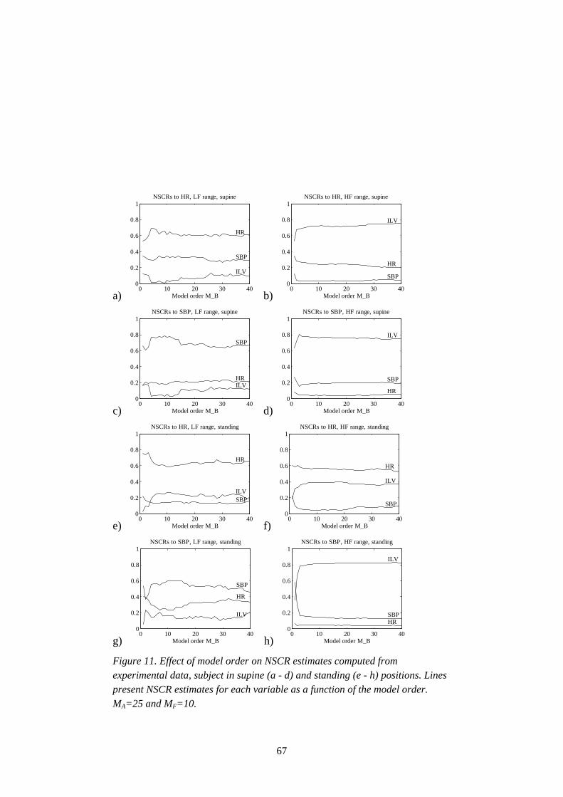
67
a)0 10 20 30 40
0
0.2
0.4
0.6
0.8
1
HR
SBP
ILV
NSCRs to HR, LF range, supine
Model order M_B b)0 10 20 30 40
0
0.2
0.4
0.6
0.8
1
HR
SBP
ILV
NSCRs to HR, HF range, supine
Model order M_B
c)0 10 20 30 40
0
0.2
0.4
0.6
0.8
1
HR
SBP
ILV
NSCRs to SBP, LF range, supine
Model order M_B d)0 10 20 30 40
0
0.2
0.4
0.6
0.8
1
HR
SBP
ILV
NSCRs to SBP, HF range, supine
Model order M_B
e)0 10 20 30 40
0
0.2
0.4
0.6
0.8
1
HR
SBPILV
NSCRs to HR, LF range, standing
Model order M_B f)0 10 20 30 40
0
0.2
0.4
0.6
0.8
1
HR
SBP
ILV
NSCRs to HR, HF range, standing
Model order M_B
g)0 10 20 30 40
0
0.2
0.4
0.6
0.8
1
HR
SBP
ILV
NSCRs to SBP, LF range, standing
Model order M_B h)0 10 20 30 40
0
0.2
0.4
0.6
0.8
1
HR SBP
ILV
NSCRs to SBP, HF range, standing
Model order M_B
Figure 11. Effect of model order on NSCR estimates computed fromexperimental data, subject in supine (a - d) and standing (e - h) positions. Linespresent NSCR estimates for each variable as a function of the model order.MA=25 and MF=10.

68
4.2.7 Interpretation of spectral decomposition analysis
Publication V showed the NSCR analysis to be robust over a large scale ofmodel orders. In addition, it is related to actual variability present in a signal.Hence, it may not be as sensitive to modelling inaccuracies due to narrow-bandsignals as is, e.g., transfer gain analysis. This makes it an attractive method forquantifying multivariate modelling results. The analysis of NSCRs enablesdecomposition of the signal spectrum into root components of different origin.Assuming a complete model, a variable yi reaches a high gain in NSCR analysisif and only if 1) the variable yi is directly influenced by an external source ofvariability (external means here some source which is not included in the modelas a variable) and 2) there exist transfer mechanisms from the variable yi toother variables yj, i≠j. Hence, an increase in the NSCR estimate from yi to yj maybe because of:
1. increased external modulation of the variable yi
2. increased gain of the transfer functions from yi to other variables (directly, orvia other variables, to yj)
3. decreased external modulation of other variables
4. decreased gain of other transfer functions than those from yi.
The NSCR analysis quantifies only the original origin of the variability and doesnot allow direct assessment of the actual transfer pathways. For example in themodels in publications III - V, the effect of respiration on HR and SBPvariability is entirely attached to the NSCRs from ILV, despite the fact thatsome of the effects may be transferred to SBP via HR (Saul et al 1991, Taylor etal 1996). The actual transfer pathways may be analysed by accompanying theNSCR analysis with, e.g., the analysis of transfer gain functions and, mostimportantly, with a priori physiological knowledge.
The NSCRs provide relative decomposition of the variability into rootcomponents. Hence, the analysis should be completed with spectral analysis toassess what the amount of actual variability in each signal and in each frequencyrange is. For example, in publication III, the NSCR analysis shows that

69
respiration is the most important origin of the DBP variability in the HF range,as it is with the HR and SBP variabilities (publication III, Figure 2). NSCRanalysis interpreted without spectral analysis might lead to the misinterpretationthat all the involved signals - HR,DBP,SBP - exhibit similar variability in thatrange. However, the spectral analysis indicates (publication III, Figure 3) thatthe variability of DBP in the HF range is much less than that of HR or SBP.This example shows that appropriate interpretation of the multivariatemodelling results requires combining information from multiple sources.
The role of pure inputs u in the model is usually more straightforward tointerpret than the role of noise sources e. The noise sources represent externalstimulations of the variable, e.g. autonomous control acting primarily on thatvariable. For example, of the variables included in the models presented in thisthesis (publications III - V), autonomous modulation of the vasculature controlsprimarily the SBP, while neural modulation of the sinus node controls primarilythe HR. Hence, an increase in the sinus node modulation should be seen as anincrease in the NSCRs from HR to other variables, and an increase in vascularmodulation as an increase in the NSCRs from SBP.
4.2.8 Limitations
Simple black-box linear modelling of a complex physiological systemnecessarily involves many deficiencies. Some of them have been mentionedabove, but here the most important ones are summarised and briefly discussed.
Nonlinearities
The cardiovascular control system and the transfer mechanisms between thedifferent variables are nonlinear. For example, baroreceptor function has beenfound to have typical sigmoid-shaped response curve to arterial pressure(Karemaker 1987), the mechanical interactions involved in heart contractionexhibit nonlinear relations between BP and RRI (run-off effect, Frank-Starlingmechanism) (Guyton 1986), respiratory sinus arrhythmia has been found to havea non-linear relation to tidal volume and respiratory frequency (Selman et al1982), etc. In addition, the relationship between HR and RRI is nonlinear(Figure 1). Because of these nonlinearities, a linear model is by default just alinear approximation of the real system dynamics. However, it has been argued

70
that a linear approximation is justified over small ranges of operation (Kitney &Gerveshi 1982, Cerutti et al 1994). This assumption is supported by studieswhich apply time series modelling in stationary short-term conditions in humansubjects and report the prediction ratio of the model: Baselli et al (1994) reportthe mean prediction ratio 75 - 84% with their linear model, while Chon et al(1996) report only 13% difference in the prediction ratio between a linear and anonlinear model. The results of the present thesis agree with these studies:prediction ratios 81 - 99% were found with linear modelling. Hence, most of thedynamics of the signals may be regressed by a linear model in stationary short-term conditions. This supports the justification of linear approximation in short-term steady-state conditions. However, the difference in nature between thenonlinear physiological system and the linear model should be recognised whenapplying the modelling.
Incompleteness of the model
In practice, it is not possible to measure all the different variables involved incardiovascular control. Hence, any time series model remains an incompleterepresentation of the true system. This hampers the interpretation of the results.If the missing variable affects only one included variable, its influence iscompletely represented by the noise source attached to that variable. However,in practice the missing variables may contribute to existing variables via variouspathways with different delays. These influences sum up to the modelledtransfer paths and noise sources in a complex way. A simultaneous externalstimulation of many variables is seen as noise source correlation, while aninfluence entering different variables with different delays is seen as an artificialtransfer mechanisms between these variables. Hence, the NSCR analysis may beaffected by variables not included in the model in a complex way. Thisemphasises the need of in-depth understanding of both the physiology and themodelling methods while interpreting the results.
Use of a priori knowledge
A priori knowledge of physiology is involved both in constructing the modeland defining the zero-delay transfer directions, and in interpreting the results.Consequently, there is a chance of biased results if the a priori knowledge is notcorrect. Hence, the modelling approach presented has limitations in yielding

71
fundamental results concerning the cardiovascular system. The most suitedapplication of the methodology is the quantification of closed-loop interactionsin various physiological or pathophysiological states where the basicmechanisms of interactions are quite well known.
Stationarity and model order selection
The time-invariant modelling presented assumes the data to be stationary. Astrue stationarity is never achieved in finite length recordings, the concept oflocal stationarity (Picinbono 1993) has to be applied: the system is studiedunder conditions during which the statistical properties of the signals do notchange. If this yields records significantly longer than the correlation time of thesystem, the recording may be assumed locally stationary (Picinbono 1993), andthe time-invariant modelling may be applied. In the cardiovascular system themaximum duration of a stationary recording is typically up to 10 minutes evenduring stable conditions. This sets certain limits on the accuracy of themodelling: the information content of a finite length recording is limited. This,in turn, sets limits for the convergence of the model with the real system (eq.12). In publication V it was found that relatively large model orders are neededto model the cardiovascular dynamics. On the other hand, the data length sets alimit for the maximal model order. An upper limit 3√N/L, where N is the datalength and L the number of variables, has been proposed for the model order(Kay 1988).
In publication V, it was shown that the NSCR estimation is not sensitive tomodel order overestimation. The same may not hold true with transfer functionanalysis or analysis of impulse responses. Increasing model order increasesvariance of the model parameters (Ljung 1987). Hence, some optimisation ofthe model order may be needed if analysis is to be extended beyond spectraldecomposition analysis.
Data quality
A factor limiting the potential of the model to describe the true system is thedata quality. This means not only a high signal-to-noise ratio but also richnessof the data from the information content point of view. Least squares modelidentification methods have most accuracy at those frequencies with most

72
spectral power and the estimates outside these frequencies are not reliable. Thecardiovascular variability signals are usually band-limited, i.e., their spectralpower is concentrated around a few frequencies. If physiologically feasible,special methods, such as broad-band respiration (Berger et al 1989b), may beused to broaden the spectral content of the signals and to overcome thisproblem. Moreover, the selection of the appropriate sampling frequency of thevariability signals is a trade-off between the time resolution and the modellingefficiency. From the time series modelling point of view, the samplingfrequency should not be higher than the time constants of the system (Ljung1987). On the other hand, increasing the sampling rate may allow more accuraterecognition of phase differences between the signals. A limiting factor in theselection of the sampling frequency is that we can obtain new samples of theheart function only at each new heart beat. The selection used in this thesis, 1Hz, may be considered appropriate as it is close to the natural rhythm of theheart at rest. While analysing real patient material, experimenting with differentsampling frequencies should be carried out to reach an appropriate trade-off.
4.2.9 Implications
Publications II - V yield some practical suggestions for the multivariatemodelling of the cardiovascular system:
• Linear multivariate time series modelling seems to provide a reasonableapproximation of the cardiovascular system during stationary short-termconditions.
• Independence of the noise sources in a closed-loop model is a pre-requisitefor the analysis of the system interactions. Dependence may causeremarkable bias in the results.
• Inclusion of the immediate transfer paths in the model is essential to makethe model noise sources independent. A simple method presented may beused to identify a MAR model with definitely independent noise sources.
• Ease of application and theoretical convergence with any linear causal time-invariant stationary system dynamics makes the MAR model an attractivemodelling tool for the cardiovascular system. However, it may not be an

73
optimal model when pure input variables (e.g. respiration) are included in themodel.
• The possible phase-lead of the HR to the ILV may cause problems in causalmodelling. Special care should be taken to control the role of respiration inthe modelling. A non-causal MARXAR structure was proposed for analysingthe effect of respiration and the closed-loop interactions between the HR andthe BP.
• Relatively high model order is needed to depict the dynamics of thecardiovascular system by linear modelling. The model order required issignificantly higher than that suggested by objective model order selectioncriteria.
• Spectral decomposition analysis and NSCR analysis provide informationabout the intersignal relationships between the cardiovascular variables. Theinformation is directly related to the actual variability present in the signals,which makes the analysis easier to interpret.
• The NSCR analysis is robust over a wide range of model orders when asufficient model order is reached and exceeded.
4.3 Author’s contribution to publications
The field of biomedical research is a multidisciplinary one and successfulresearch in the area demands the collaboration of researchers from differentfields. Because of that, this thesis work has been carried out partly at VTTInformation Technology (the former Medical Engineering Laboratory of theTechnical Research Centre of Finland) and partly at the Department of ClinicalPhysiology, Tampere University Hospital. The research work described hasbeen carried out in very close co-operation with the clinicians, and part of thestudy (publication I) has been managed by them at Tampere UniversityHospital.
In publication I the author was the only technical expert participating in theanalysis carried out. The author had the main responsibility for designing and

74
defining the analysis methods and he authored the analysis software. Especially,the author proposed the use of high-order AR spectral estimation and the use offMED to quantify the frequency shift on the LF band.
In publications II-V the author has been the principle author. In publication IIthe author elaborated the presentation of the general linear stochastic time seriesmodelling framework for physiological signal analysis. The co-authorspresented the multivariate dynamic adjustment and time-variant modelling partsof the paper (chapters 2.4.2 and 2.4.3). In publication III the author carried outthe MAR modelling case, including laboratory measurements, data processing,modelling and analysis, and was the main author of the introduction anddiscussion. The presentation of the multivariate dynamic and time-variantmodelling parts (chapters 2.2 and 2.3) was carried out by the co-authors. Inpublication IV the author proposed the application of the Choleskydecomposition method to make the noise sources of the model mutuallyindependent, designed the study set-up, participated in the laboratorymeasurements, authored the analysis software, performed the data analysis anddrew the main conclusions. Publication V was the work solely of the author, butin collaboration with the clinicians from Tampere University Hospital.

75
5. General discussion and conclusions
The spectral analysis of cardiovascular variability signals has been underintensive research for three decades. These analyses are gradually reaching thestage of clinical applications, and the methods are becoming more standardised.Yet, application of spectral analysis for research or clinical purposes needsspecial care to be taken in order for proper methodologies to be used. Despitesome recommendations published recently (Task Force of ESC & NASPE1996), all the details of analysis can often not be defined without an in-depthknowledge of the methods. For example, when using AR spectral estimation, noclear rule-of-thumb can be given for the model order selection. This thesis, andsome other reports published in the recent past (Kay 1988, Pinna et al 1996),criticise the straightforward use of certain objective criteria in the model orderselection. The existence of these kinds of open methodological questionsunderlines the importance of co-operation between physicians and engineers inthe analysis of cardiovascular variability signals.
Because of long-lasting and intensive research in the spectral analysis ofcardiovascular variability signals, no revolutionary methodological findingswere expected. Usually, the spectral analysis is carried out by analysing thespectral power in certain pre-defined frequency ranges. Our experimentalfinding in Takalo et al 1994a and publication I was that in BHT subjects there isa shift in the frequency of oscillations inside the LF band. This shift may not bedetected by conventional analysis of spectral power only. This emphasises theneed for methods to quantify also the frequency of oscillations in addition totheir power. In this thesis, three methods were compared to quantify thisspectral shift. The outcome was the principle result of this thesis in univariatespectral analysis: band-wise fMED and fMEAN provide more robust quantificationof this shift than the fC which has been used in various previous studies.
Multivariate modelling has been addressed as one of the most promisingapproaches to the analysis of cardiovascular variability signals (Task Force ofESC & NASPE 1996). In this thesis some efforts were made to bring themethodology towards application in clinical research. The model identificationprocedures and the parametrisation of the modelling results were designed forthis purpose. Still, when applying the methods to real experimental data, itshould be kept in mind that the approach presented is designed more to draw

76
quantitative parameters related to the functioning of the cardiovascular controlsystem than to be a realistic model of the underlying system. In particular, oneshould bear in mind the limitations in the performance of the linear models, themost important of which are related to the demands for stationarity, appropriatedata length and quality and justification of the linearity assumption in differentcircumstances. The system identification cycle presented in publication IIshould always be followed in order to guarantee that the results obtained arecorrectly interpreted.
Insensitivity of spectral decomposition analysis to the changes in model order isa useful characteristic. The selection of model order is considered one of themost difficult problems in multivariate modelling. An important fact came tolight: when multivariate modelling is used for data description rather thancontrol purposes, it is not harmful to overestimate the model order within limits,but an underestimation may yield erroneous results. In publication V, asaturation of the NSCR estimates at a certain level was found when the modelorder was increased. This was true for both the simulation and the experimentaldata. If this is a general phenomenon with cardiovascular variability data, itmight be utilised as a foundation for developing a simple model order selectioncriterion.
At present, only spectral decomposition analysis was applied for the analysis ofinteractions. In the future, use of other parameters like transfer functions andimpulse responses should be considered and their behaviour in relation to theselected model order should be studied. In addition, the frequency content of thespectral decomposition might be studied using parameters such as fMED or fMEAN,as with the univariate spectral analysis. These studies might define other robustparameters to describe the model dynamics. Another interesting researchdirection in the analysis of the cardiovascular control system would be theconsideration of other variability signals in addition to HR, BP and respiration.Recently, advances in impedance cardiography have greatly improved itsreliability, and there exist devices which allow non-invasive beat-to-beatmonitoring of SV (Kööbi et al 1997). This allows direct measurement of one ofthe most important variables in the dynamics of the cardiovascular system andhence could yield significant new insights into the control system. The methodspresented in this thesis may be adapted with minor modifications to include SVor any other related signal.

77
In the present thesis, the multivariate modelling methods developed wereapplied to real experimental data only for demonstration purposes. In futurestudies, the methods should be validated against real physiological data from arelatively large number of subjects. Only after that can the methods presentedconsidered valid and reliable.
In this thesis, a new parameter for quantifying spectral shift in HR and BPsignals, namely band-wise median frequency, or fMED, was proposed and appliedto the analysis of experimental data from BHT and HT subjects. In addition, ageneral framework for multivariate linear modelling of cardiovascular signalswas presented. The use of spectral decomposition for analysing the intersignalrelationships in the model and methods for enhancing the MAR modelling wereproposed. Finally, a new type of linear model for modelling cardiovasculardynamics was introduced. Identification procedures relying on generallyavailable software tools were developed both for the new MAR model form andfor the MARXAR model. The behaviour of the models was analysed, and theeffect of model order selection was analysed with the MARXAR model. It maybe concluded that the multivariate modelling approach was developedsufficiently to allow its future application to experimental data sets.

78
References
AAMI. 1989. Apnea monitoring by means of thoracic impendancepneumography (AAMI TIR No. 4-1989). AAMI, Arlington, Virginia, USA.
Akaike H. 1974. A new look at the statistical model identification. IEEE TransAutom Contr, AC-19:716-723.
Akkerman EM, Karemaker JM, Strackee J. 1995. Computer modelling thedynamics of the circulation under gravitational stress. In: Di Rienzo M, ManciaG, Parati A, Pedotti A, Zanchetti A (eds.). Computer analysis of blood pressureand heart rate signals, IOS Press, Amsterdam, Netherlands. Pp. 135-150.
Akselrod S, Gordon D, Ubel FA, Shannon DC, Berger AC, Cohen RJ. 1981.Power spectrum analysis of heart rate fluctuation: a quantitative probe of beat-to-beat cardiovascular control. Science, 213: 220-222.
Akselrod S, Gordon D, Madwed JB, Snidman NC, Shannon DC, Cohen RJ.1985. Hemodynamic regulation: investigation by spectral analysis. Am JPhysiol, 249:H867-H875.
Anderson EA, Sinkey CA, Lawton WJ, Mark AL. 1989. Elevated sympatheticnerve activity in borderline hypertensive humans: evidence from directintraneural recordings. Hypertension, 14:177-183.
Appel ML, Saul JP, Berger RD, Cohen RJ. 1989. Closed-loop identification ofcardiovascular regulatory mechanisms. Comp Cardiol, 16:3-7.
Appel ML, Saul JP, Berger RD, Cohen RJ. 1993. Closed-loop identification ofblood pressure variability mechanisms. In: Di Rienzo M, Mancia G, Parati G,Pedotti A, Zanchetti A (Eds.): Blood pressure and heart rate variability. IOSPress, Amsterdam, the Netherlands. Pp. 68-74.

79
Barbieri R, Di Virgillio V, Triedman JK, Bianchi AM, Cerutti S, Saul JP. 1995.Multivariate autoregressive spectral analysis: heart rate baroreflex amdrespiratory influence under administration of atropine and propranonol. In:IEEE Engineering in Medicine and Biology 17th Annual Confrence, Montreal,Canada.
Barbieri R, Triedman JK, Di Virgillio V, Cerutti S, Saul JP. 1996a. Arterialpressure control during non-hypo/hypertensive changes in central venousvolume: assessment with multivariate autoregressive modeling. In: IEEEComputers in Cardiology, Indianapolis, Indiana, USA.
Barbieri R, Waldman RA, Di Virgilio V, Triedman JK, Bianchi AM, Cerutti S,Saul JP. 1996b. Continuous quantification of baroreflex and respiratory controlof heart rate by use of bivariate autoregressive techniques. Ann NoninvElectrocardiol, 1(2):264-277.
Baselli G, Cerutti S. 1985. Identification techniques applied to processing ofsignals from cardiovascular systems. Med Inform, 10(3):223-235.
Baselli G, Cerutti S, Civardi S, Liberati D, Lombardi F, Malliani A, Pagani M.1986. Spectral and cross-spectral analysis of heart rate and arterial bloodpressure variability signals. Comp Biomed Res, 19:520-534.
Baselli G, Cerutti S, Civardi S, Lombardi F, Malliani A, Merri M, Pagani M,Rizzo G. 1987. Heart rate variability signal processing: a quantitative approachas an aid to diagnosis in cardiovascular pathologies. Int J Bio-Med Comp,20:51-70.
Baselli G, Cerutti S, Livraghi M, Meneghini C, Pagani M, Rimoldi O. 1988a.Causal relationship between heart rate and arterial blood pressure variabilitysignals. Med Biol Eng Comp, 26:374-378.
Baselli G, Cerutti S, Civardi S, Malliani A, Pagani M. 1988b. Cardiovascularvariability signals: towards the identification of a closed-loop model of theneural control mechanisms. IEEE Trans Biomed Eng, 35:1033-1046.

80
Baselli G, Cerutti S, Badilini F, Biancardi L, Porta A, Pagani M, Lombardi F,Rimoldi O, Furlan R, Malliani A. 1994. Model for the assessment of heartperiod and arterial pressure variability interactions and of respiration influences.Med Biol Eng Comp, 32:143-152.
Bendat JS, Piersol AG. 1986. Random data. Analysis and measurementprocedures. 2nd edition. John Wiley & Sons, Inc., USA. 566 p.
Bennett T, Farquhar IK, Hosking DJ, Hampton JR. 1978. Assessment ofmethods for estimating autonomic nervous control of heart in patients withdiabetes mellitus. Diabetes, 27:1167-1174.
Bennett FM, Christini DJ, Ahmed H, Lutchen K, Hausdorff JM, Oriol N. 1993.Time series modeling of heart rate dynamics. In: IEEE Computers inCardiology, London, United Kingdom. Pp. 273-276.
Berger RD, Akselrod S, Gordon D, Cohen RJ. 1986. An efficient algorithm forspectral analysis of heart rate variability. IEEE Trans Biomed Eng 33(9):900-904.
Berger RD, Saul JP, Cohen RJ. 1989a. Transfer function analysis of autonomicregulation. I. Canine atrial rate response. Am J Physiol, 1989; 256:H142-H152.
Berger RD, Saul JP, Cohen RJ. 1989b. Assessment of autonomic response bybroad-band respiration. IEEE Trans Biomed Eng, 36(11):1061-1065. (Erratum:IEEE Trans Biomed Eng, 37(1):112.)
Bianchi A, Mainardi L, Petrucci E, Signorini M, Mainardi M, Cerutti S. 1993.Time-variant power spectrum analysis for the detection of transient episodes inHRV signal. IEEE Trans Biomed Eng, 40:136-144.
Bigger JT Jr, Steinman RC, Rolnitzky LM, Fleiss JL, Albrecht P, Cohen RJ.1996. Power law behavior of RR-interval variability in healthy middle-agedpersons, patients with recent acute myocardial infarction, and patients with hearttransplants. Circulation, 93(12):2142-2151.

81
Braunwald E, Ross J Jr, Sonnenblick EH. 1967. Mechanisms of contraction ofthe normal and failing heart. N Eng J Med, 277:853-863.
Burton AC, Taylor D. 1940. A study of the adjustment of peripheral vasculartone to the requirements of body temperature. Am J Physiol, 129:565-577.
Castiglioni P. 1995. Evaluation of heart rhythm variability by heart rate or heartperiod: differences, pitfalls and help from logarithms. Med Biol Eng Comp,33:323-330.
Cerutti S, Baselli G, Bianchi AM, Mainardi LT, Signorini MG, Malliani A.1994. Cardiovascular variability signals: from signal processing to modellingcomplex physiological interactions. Automedica, 16:45-69.
Cerutti S, Signorini MG. 1996. The heart rate variability signal: among rhythms,noise and chaos. In: Gath I, Ingbar GF (eds). Advances in Processing andPattern Analysis of Biological Signals, Plenum Press,New York. Pp. 235-249.
Chon KH, Mullen TJ, Cohen RJ. 1996. A dual-input nonlinear system analysisof autonomic modulation af heart rate. IEEE Trans Biomed Eng, 43(5):530-544.
Cyon E. 1874. Zur Physiologie des Gefässnervencentrums. Pflüger’s Arch,9:499-513.
deBoer RW, Karemaker JM, Strackee J. 1984. Comparing spectra of a series ofpoint events particularly for heart rate variability data. IEEE Trans Biomed Eng,31(4):384-387.
deBoer RW, Karemaker JM, Strackee J. 1985. Relationships between short-termblood-pressure fluctuations and heart rate variability in resting subjects. I.Spectral analysis approach. Med Biol Eng Comp, 23:352-358.
deBoer RW, Karemaker JM, Strackee J. 1987. Hemodynamic fluctuations andbaroreflex sensitivity in humans: a beat-to-beat model. Am J Physiol, 253:680-689.

82
DeGroot MH. 1975. Probability and Statistics. Addison-Wesley, Reading, MA,USA.
DeLuca C. 1985. Myoelectric manifestations of localized muscle fatigue inhumans. CRC Crit Rev Biomed Eng, 11:251-279.
di Rienzo M, Castiglioni P, Mancia G, Parati G, Pedotti A. 1989. 24 hsequential spectral analysis of arterial blood pressure and pulse interval in free-moving subjects. IEEE Trans Biomed Eng, 36(11):1066-1075.
Eckberg DL, Nerhed C, Wallin BG. 1985. Respiratory modulation of musclesympathetic and vagal cardiac outflow in man. J Physiol (London), 365:181-196.
Eckberg DL, Sleight P. 1992. Human baroreflexes in health and disease. OxfordUniversity Press, New York, USA.
Eckberg DL. 1995. Respiratory sinus arrhythmia and other humancardiovascular neural periodocities. In: Lenfant C, Pack A, Dempsey JA (eds.).Regulation of Breathing, 2nd Edition. Marcel-Dekker, New York, USA. Pp.669-740.
Fallen EL, Kamath MV, Ghista DN, Fitchett D. 1988. Spectral analysis of heartrate variability following human heart transplantation: evidence for functionalreinnervation. J Auton Nerv Syst, 23:199-206.
Fredericq L. 1882. De l’influence de la respiration sur la circulation. Lesoscillations respiratoires de la pression artérielle chez le chien. Arch Biol Paris3:55-100.
Freeman R, Cohen RJ, Saul JP. 1995. Transfer function analysis of respiratorysinus arrhythmia: a measure of autonomic function in diabetic neuropathy.Muscle & Nerve, 18:74-84.
Gleick J. 1987. Chaos: Making a New Science. Viking Penguin, New York,USA.

83
Grönlund JU, Kalli S, Siimes ASI, Sydänmaa M, Antila KJ, Välimäki I. 1991.Do β-adrenergic blockade and sleep state affect cardiorespiratory control inneonatal lambs? Multivariate autoregressive modeling approach. PediatricResearch, 29:272-277.
Grönlund JU, Jalonen J, Korhonen I, Rolfe P, Välimäki IT. 1995. Multivariateautoregressive modelling combined with transcephalic electrical impedance:method to relate neonatal systemic circulation and respiration to cerebralcirculation. Med Biol Eng Comp, 33:458-463.
Guyton AC. 1986. Textbook of medical physiology. WB Saunders, London,United Kingdom.
Guzzetti S, Piccaluga E, Casati R, Cerutti S, Lombardi F, Pagani M, Malliani A.1988. Sympathetic predominance in essential hypertension: a study employingspectral analysis of heart rate variability. J Hypertension, 6:711-717.
Hales S. 1733. Statical essays: containing haemastatics; or, an acount of somehydraulick and hydrostatical experiments made on the blood and blood-vesselsof animals. Innys W, Manby R, Woodward T. London, United Kingdom.
Haller A. von. 1778. De partium corporis humani praecipuarum fabrica etfunctionibus. Berne: Prelis Societatum Typhograhicarum.
Hannan EJ, Deistler M. 1988. The statistical theory of linear systems. JohnWiley & Sons, Inc., New York, USA. 380 p.
Hayano J, Yamada M, Sakakibara Y, Fujinami T, Yokoyama K, Watanabe Y,Takata K. 1990. Short- and long-term effects of cigarette smoking on heart ratevariability. Am J Cardiol, 65:84-88.
Hayano J, Taylor JA, Yamada A, Mukai S, Hori R, Asakawa T, Yokoyama K,Watanabe Y, Takata, K, Fujinami T. 1993. Continuous assessment ofhemodynamic control by complex demodulation of cardiovascular variability.Am J Physiol, 264:H1229-H1238.

84
Hering E. 1869. Über den Einfluss der Atmung auf den Kreislauf I. ÜberAthembewegungen des Gefässsystems. Sitzungsberichte Mathemat-Naturwissenschaft Classe Kaiserlich Akad Wissenschaft, 60:829-856.
Hon EH, Lee ST. 1963. Electronic evaluation of the fetal heart rate. VIII.Patterns preceding fetal death, further observations. Am J Obstet Gynecol,87:814-826.
Hyndman BW, Kitney RI, Sayers BMcA. 1971. Spontaneous rhythms inphysiological control systems. Nature, 233:339-41.
Hägg GM. 1991. Comparison of different estimators of electromyographicspectral shifts during work when applied on short test conditions. Med Biol EngComp, 29:511-516.
Japundiz N, Grichois M-L, Zitoun P, Laude D, Elghozi J-L. 1990. Spectralanalysis of blood pressure and heart rate in conscious rats: effects of autonomicblockers. J Auton Nerv Syst, 30:91-100.
Jorna PGAM. 1985. Heart rate parameters and the coping process underwater.In: Orlebeke JF, Mulder G, van Doornen LJP (Eds.). Psychophysiology ofcardiovascular control: methods, models and data. Plenum, New York, USA.
Jorna PGAM. 1992. Spectral analysis of heart rate and physiological state: areview of its validity as a workload index. Biol Psychol, 34:237-257.
Julius S. 1991. Autonomic nervous system dysregulation in humanhypertension. Am J Cardiol, 67:3B-7B.
Kailath T. 1985. Linear estimation for stationary and near-stationary processes.In: Kailath T. (Ed.): Modern Signal Processing, Hemisphere PublishingCorporation, New York, USA. Pp. 59-122.
Kalli S, Suoranta R, Jokipii M. 1986. Applying a multivariate autoregressivemodel to describe interactions between blood pressure and heart rate. In:Measurement in clinical medicine. The institute of measurement and control,London. Pp. 77-82.

85
Kalli S, Grönlund J, Ihalainen H, Siimes A, Välimäki I, Antila K. 1988a.Multivariate autoregressive modeling of cardiovascular control in neonatallamb. Comp Biomed Res, 21:512-530.
Kalli S, Turjanmaa V, Suoranta R, Uusitalo A. 1988b. Assesment of bloodpressure and heart rate variability using multivariate autoregressive modelling.Biomed Meas Inf Contr, 2:46-56.
Kamath MV, Fallen EL. 1993. Power spectral analysis of heart rate variability:a noninvasive signature of cardiac autonomic function. Critical Reviews BiomedEng, 21(3):245-311.
Kamath MV, Fallen EL. 1995. Correction of the heart rate variability signal forectopic and missing beats. In: Malik M, Camm AJ (eds). Heart RateVariability. Futura, Armonk, New York, USA. Pp. 75-85.
Kaplan DT, Furman MI, Pincus SM, Ryan SM, Lipsitz LA, Goldberger AL.1991. Aging and the complexity of cardiovascular dynamics. Biophys J, 59:945-949.
Karemaker JM. 1987. Neurophysiology of the baroreceptor reflex. In: KitneyRI, Rompelman (eds). The beat-to-beat investigation of cardiovascular function.Measurement, analysis, and applications. Oxford University Press, Oxford, UK.Pp. 27-49.
Kay SM. 1988. Modern spectral estimation: theory and application. Prentice-Hall, Inc., Englewood Cliffs, New Jersey, USA. 543 p.
Kirchheim HR. 1977. Systemic arterial baroreflexes. Physiol Rev, 56:100-176.
Kitney RI. 1979. A non-linear model for studying oscillations in the bloodpressure control system. J Biomed Eng, 1:89-99.
Kitney RI, Byrne S, Edmonds ME, Watkins PJ, Roberts VC. 1982. Heart ratevariability in the assessment of autonomic diabetic neuropathy. Automedica,4:155-167.

86
Kitney RI, Gerveshi CM. 1982. System identification of the blood pressurecontrol system by low frequency neural stimulation. Trans Inst M C, 4:203-212.
Kitney RI, Fulton T, McDonald AH, Linkens DA. 1985. Transient interactionsbetween blood pressure, respiration and heart rate in man. J Biomed Eng, 7:217-224.
Kitney RI, Darvish N. 1995. Techniques for studying short-term changes incardio-respiratory data, II. In: Di Rienzo M, Mancia G, Parati G, Pedotti A,Zanchetti A (eds.). Computer Analysis of Cardiovascular Signals. IOS Press,Amsterdam, the Netherlands. Pp. 15-52.
Korhonen I, Turjanmaa V. 1995. Second-order non-linearity of heart rate andblood pressure short-term variability. In: IEEE Computers in Cardiology, Wien,Austria. Pp. 293-296.
Kleiger RE, Miller JP, Bigger JT, Moss AJ, and Multicenter Post-InfarctionResearch Group. 1987. Decreased heart rate variability and its association withincreased mortality after acute myocardial infarction. Am J Cardiol, 59:256-262.
Kööbi T, Kaukinen S, Turjanmaa VMH, Uusitalo A. 1997. Whole-bodyimpedance cardiography in the measurement of cardiac output. Crit Care Med,in press.
Landers TE, Lacoss RT. 1977. Some geophysical applications of autoregressivespectral estimates. IEEE Trans Geosci Electron, 15:26-32.
Leaning MS, Pullen HE, Carson ER, Finkelstein L. 1983. Modelling a complexbiological system: the human cardiovascular system - 1. Methodology andmodel description. Trans Inst M C, 5(2):71-86.
Levy MN. 1971. Sympathetic-parasympathetic interactions in the heart. CircRes, 29:437-445.
Lindström L, Magnusson R, Petersen I. 1970. Muscular fatigue and actionpotential conduction velocity changes studied with frequency analysis of EMGsignals. Electromyography, 10:341-356.

87
Ljung L. 1987. System identification. Theory for the user. Prentice-Hall, Inc.,Englewood Cliffs, New Jersey, USA. 519 p.
Loula P, Lipping T, Jäntti V, Yli-Hankala A. 1994. Nonlinear interpretation ofrespiratory sinus arrhytmia in anesthesia. Meth Inf Med, 33:52-57.
Luczag H, Laurig W. 1973. An analysis of heart rate varibility. Ergonomics,16:85-97.
Ludwig C. 1847. Beiträge zur Kennthiss des Einflusses derRespirationsbewegungen auf den Blutlauf im Aortensysteme. Muller’s ArchAnat Physiol Med, 242-302.
Mainardi LT, Bianchi AM, Barbieri R, Di Virgilio V, Piazza S, Furlan R,Baselli G, Cerutti S. 1993. Time-variant closed-loop interaction between HRand ABP variability signals during syncope. In: IEEE Computers in Cardiology,London. Pp. 699-702.
Mainardi LT, Bianchi AM, Baselli G, Cerutti S. 1995. Pole-tracking algorithmsfor the extraction of time-variant heart rate variability spectral parameters. IEEETrans Biomed Eng, 42(3):250-259.
Malliani A, Pagani M, Lombardi F, Cerutti S. 1991. Cardiovascular neuralregulation explored in the frequency domain. Circulation, 84(2):482-492.
Marmarelis VZ. 1993. Identification of nonlinear biological systems usinglaguerre expansions of kernels. Ann Biomed Eng, 21:573-589.
Marple SL. 1987. Digital spectral analysis with applications. Prentice-Hall, Inc.,Englewood Cliffs, New Jersey, USA. 492 p.
Mayer S. 1877. Studien zur Physiologie des Herzens und der Blutgefässe. V.Über spontane Blutdruckschwankungen. Sitzungsberichte Kaiserlich AkadWissenschaft Mathemat-Naturwissenschaft Classe, 74:281-307.

88
Merri M, Farden DC, Mottley JG, Titlebaum EL. 1990. Sampling frequency ofthe electrocardiogram for spectral analysis of heart rate variability. IEEE TransBiomed Eng, 37(1):99-106.
Mullen TJ, Appel ML, Mukkamala R, Mathias JM, Cohen RJ. 1997. Systemidentification of closed-loop cardiovascular control mechanisms: pharmacologicautonomic blockade and postural effects. Am J Physiol, in press.
Novak P, Novak V. 1993. Time/frequency mapping of the heart rate, bloodpressure and respiratory signals. Med Biol Eng Comput, 31:103-110.
Oguma R. 1981. Method to evaluate signal transmission paths in dynamicsystems and its application to reactor noise analysis. J Nuc Sci Tech, 18:835-844.
Oguma R. 1982. Extended partial and multiple coherence analyses and theirapplication to reactor noise investigation. J Nuc Sci Tech, 19:543-554.
Omboni S, Parati G, Frattola A, Mutti E, Di Rienzo M, Castiglioni P, Mancia G.1993. Spectral and sequence analysis of finger blood pressure variability:comparison with analysis of intra-arterial recordings. Hypertension, 22:26-33.
Pagani M, Lombardi F, Guzzetti S, Rimoldi O, Furlan R, Pizzinelli P, SandroneG, Malfatto G, Dell'Orto S, Piccaluga E, Turiel M, Baselli G, Cerutti S, MallianiA. 1986. Power spectral analysis of a beat-to-beat heart rate and blood pressurevariability as a possible marker of sympatho-vagal interaction in man andconscious dog. Circ Res, 59:178-193.
Pagani M, Somers V, Furlan R, Dell’Orto S, Conway J, Baselli G, Cerutti S,Sleight P, Malliani A. 1988. Changes in autonomic ragulation induced byphysical training in mild hypertension. Hypertension, 12:600-610.
Parati G, Di Rienzo M, Bertinieri G, Pomidossi G, Casadei R, Groppelli A,Pedotti A, Zanchetti A, Mancia G. 1988. Evaluation of the baroreceptor-heartrate reflex by 24-hour intra-arterial blood pressure monitoring in humans.Hypertension, 12:214-222.

89
Penaz J. 1973. Photoelectric measurement of blood pressure, volume and flowin the finger. In: Digest of 10th International Conference on Medical andBiological Engineering , Dresden, Germany. P. 104.
Perrott MH, Cohen RJ. 1996. An efficient approach to ARMA modeling ofbiological systems with multiple inputs and delays. IEEE Trans Biomed Eng,43:1-14.
Picinbono B. 1993. Random signals and systems. Prentice Hall, EnglewoodCliffs, New Jersey, USA. 591 p.
Pinna GD, Maestri R, Di Cesare A. 1996. Application of time series spectralanalysis theory: analysis of cardiovascular variability signals. Med Biol EngComp, 34:142-148.
Poiseuille JLM. 1828. Recherches sur la force du coeur aortique. Extraites desTheses soutennues dans les Trois Facultes de Medicine de France, Arch GenMed, 18:550-555.
Pola S, Marchesi C, Macerata A, Edmin M. 1995. Assessing variability incardiovascular series during autonomic tests. In: Di Rienzo M, Mancia G, ParatiG, Pedotti A, Zanchetti A (eds.). Computer Analysis of Cardiovascular Signals.IOS Press, Amsterdam, the Netherlands. Pp. 53-66.
Porges SW, Bohrer RE, Cheung MN, Drasgow F, McCabe PM, Keren G. 1980.New time-series statistic for detecting rhytmic co-occurrence in the frequencydomain: the weighted coherence and its application to psychophysiologicalresearch. Psychol Bulletin, 88(3):580-587.
Rea RF, Eckberg DL. 1987. Carotid baroreceptor-muscle sympathetic relation inhumans. Am J Physiol, 253:R929-R934.
Robbe HWJ, Mulder LJM, Rüddel H, Langewitz WA, Veldman JBP, Mulder G.1987. Assessment of barorecptor reflex sensitivity by means of spectralanalysis. Hypertension, 10: 538-543.

90
Rompelman O, Snijders JBIM, Van Spronsen CJ. 1982. The measurement ofheart rate variability spectra with the help of a personal computer. IEEE TransBiomed Eng, 29:503-510.
Rompelman O. 1986. Tutorial review on processing the cardiac event series: asignal analysis approach. Automedica, 7:191-212.
Rompelman O, Tenvoorde BJ. 1995. Spectral analysis of fluctuations in heartrate and blood pressure. In: Di Rienzo M, Mancia G, Parati G, Pedotti A,Zanchetti A. (Eds.): Computer analysis of cardiovascular signals. IOS Press,Amsterdam, Netherlands. Pp. 3-13.
Roy M, Stephoe A. 1991. The inhibition of cardiovascular responses to mentalstress following aerobic exercise. Psychophysiology, 6:689-700.
Saranummi N, Korhonen I, van Gils M, Kari A. 1997. Framework for biosignalinterpretation in intensive care and anaesthesia. Meth Inform Medicine, in press.
Saul JP, Berger RD, Chen MH, Cohen RJ. 1989. Transfer function analysis ofautonomic regulation II. Respiratory sinus arrhythmia. Am J Physiol, 256:H153-61.
Saul JP, Rea RF, Eckberg DL, Berger RD, Cohen RJ. 1990. Heart rate andmuscle sympathetic nerve variability during reflex changes of autonomicactivity. Am J Physiol, 258:H713-H721.
Saul JP, Berger RD, Albrecht P, Stein SP, Chen MH, Cohen RJ. 1991. Transferfunction analysis of circulation: unique insights into cardiovascular regulation.Am J Physiol, 261: H1231-H1245.
Sayers BMcA. 1973. Analysis of heart rate variability. Ergonomics, 16:17-32.
Schmidt RF, Thews G. 1983. Human physiology. Springer-Verlag, Berlin,Germany; 1983, 397-454.

91
Scholz UJ, Bianchi AM, Cerutti S, Kubicki S. 1993. Monitoring of thevegetative background of sleep by means of spectral analysis of heart ratevariability. In: IEEE Computers in Cardiology, London, United Kingdom. Pp.321-324.
Schweitzer A. 1945. Rhytmical fluctuations of the arterial blood pressure. JPhysiol, London, 104:25P-26P.
Schweitzer TW, Fitzgerald JW, Bowden JA, Lynne-Davies P. 1979. Spectralanalysis of human inspiratory diaphragmatic electromyograms. J Appl Physiol:Respirat Environ Exercise Physiol, 46:152-165.
Selman AC, McDonald AH, Kitney RI, Linkens DA. 1982. The interactionbetween heart rate and respiration: Part I: Experimental studies in man.Automedica, 4:131-139.
Shin S-J, Tapp WN, Reisman SS, Natelson BH. 1989. Assessment of autonomicregulation of heart rate variability by the method of complex demodulation.IEEE Trans Biomed Eng, 36(2):274-283.
Smith JJ, Kampine JP. 1980. Pressure and flow in the arterial and venoussystems. In: Smith JJ, Kampine JP. (eds.): Circulatory Physiology: theEssentials. Williams & Wilkins, Baltimore, Maryland, USA. Pp. 53-75.
Stulen FB, DeLuca CJ. 1981. Frequency parameters of the myoelectric signal asa measure of muscle conduction velocity. IEEE Trans Biomed Eng, 28:515-523.
Suoranta R. 1990. Analysis of linear systems applying multivariateautoregressive model. Licentiate Thesis, Tampere University of Technology,Tampere, Finland. 83 p.
Suoranta R, Rantala S. 1991. Utilizing multivariate autoregressive model toreveal internal dependencies in multichannel measurement data. In: Proceedingsof the IEEE Instrumentation and Measurement Technology Conference, Atlanta,USA. Pp. 315-318.

92
Suoranta R. 1995. Amplitude domain approach to digital filtering. Theory andapplications of L-filters. VTT Publications 248, Technical Research Centre ofFinland, Espoo. 199 p.
Takalo R, Korhonen I, Turjanmaa V, Majahalme S, Tuomisto M, Uusitalo A.1994a. Short-term variability of blood pressure and heart rate in borderline andmild hypertensives. Hypertension, 23(1):18-24.
Takalo R, Korhonen I, Turjanmaa V, Majahalme S, Uusitalo A. 1994b.Importance of appropriate spectral methodology to assess heart rate variabilityin the frequency domain. Response to 'Letter to the Editor’. Hypertension,24(1): 140-142.
Task Force of the European Society of Cardiology (ESC) and the NorthAmerican Society of Pacing and Electrophysiology (NASPE). 1996. Heart ratevariability. Standards of measurement, physiological interpretation, and clinicaluse. Circulation, 93:1043-1065.
Taylor JA, Hayano J, Seals DR. 1995. Lesser vagal withdrawal during isometricexercise with age. J Appl Physiol, 79(3):805-811.
Taylor JA, Eckberg DL. 1996. Fundamental relations between short-term RRinterval and arterial pressure oscillations in humans. Circulation, 93:1527-1532.
TenVoorde BJ, Faes ThJC, Rompelman O. 1994. Spectra of data sampled atfrequency-modulated rates in application to cardiovascular signals: Part 2evaluation of Fourier transform algorithms. Med Biol Eng Comp, 32:71-76.
TenVoorde BJ, Faes ThJC, Janssen TWJ, Scheffer GJ, Rompelman O. 1995.Respiratory modulation of blood pressure and heart rate studied with a computermodel of baroreflex control. In: Di Rienzo M, Mancia G, Parati G, Pedotti A,Zanchetti A (eds.). Computer Analysis of Cardiovascular Signals. IOS Press,Amsterdam, the Netherlands. Pp. 119-134.
Toska K. 1995. Short-term cardiovascular control in humans. Doctoral thesis,University of Oslo, Oslo, Norway. 84 p. + 4 app.

93
Traube L. 1865. Über periodische Thätigkeits-Aeusserungen desvasomotorischen und Hemmungs-Nervencentrums. Centralbl Med Wissenschaft,56:881-885.
Triedman JK, Cohen RJ, Saul JP. 1993. Mild hypovolemic stress altersautonomic modulation of heart rate. Hypertension, 21:236:247.
Triedman JK, Perrott MH, Cohen RJ, Saul JP. 1995. Respiratory sinusarrhythmia: time domain characterization using autoregressive moving averageanalysis. Am J Physiol, 268:H2232-H2238.
Tulppo MP, Mäkikallio TH, Takala TES, Seppänen T, Huikuri HV. 1996.Quantitative beat-to-beat analysis of heart rate dynamics during exercise. Am JPhysiol, 271:H244-H252.
Turjanmaa V, Kalli S, Sydänmaa M, Uusitalo A. 1990. Short-term variability ofsystolic blood pressure and heart rate in normotensive subjects. Clin Physiol,10:389-401.
Upadhyaya B, Kitamura M, Kerlin T. 1980. Multivariate signal analysisalgorithms for process monitoring and parameter estimation in nuclear reactors.Ann Nuc Energy, 7:243-247.
Wallin BG, Burke D, Gandevia S. 1994. Coupling between variations instrength and baroreflex latency of sympathetic discharges in human musclenerves. J Physiol (London), 474:331-338.
Vermeiren C, Médigue C, Bourgin P, Debouzy C, Escourrou P. 1995a.Automated feature extraction on polygraphic recordings: cardiovascularperturbations during nocturnal periodig leg movements. In: IEEE Engineering inMedicine and Biology 17th Annual Confrence, Montreal, Canada. Pp. 957-958.
Vermeiren C, Escourrou P, Papelier Y, Le Vey G, Przybyszewski AW. 1995b.Assessment of the phase relationship between breathing, heart rate and bloodpressure by the modified complex demodulation. In: IEEE Engineering inMedicine and Biology 17th Annual Confrence, Montreal, Canada. Pp. 943-944.

94
WHO Expert Committee. 1978. Arterial Hypertension. Geneva, Switzerland,World Health Organisation. P. 8.
Värri AO, Grote L, Penzel T, Cassel W, Peter JH, Hasan J. 1994. A new methodto study blood pressure, heart rate and EEG as a function of reaction time. MethInform Med, 33:64-67.
Yamamoto Y, Hughson RL, Peterson JC. 1991. Autonomic control of heart rateduring exercise studied by heart rate variability spectral analysis. J ApplPhysiol, 71(3):1136-1142
.

Errata in publications
Publication II, page 2, 3rd paragraph:
We divided the spectrum into three bands because it has beenshown that the short-term variability in HR is affected by threemajor physiological factors attributable to respiratory, pressurevasomotor (at around 0.1 Hz) and thermal vasomotor (at around0.05 Hz) activities. There is evidence that even the renin-angiotensin system may play a significant role in short-termcardiovascular control (at around 0.04 Hz). So there are certainlymore than two oscillations involved in BP and HR variabilityabove 0.03 Hz.
Publication II, equation 1:
A y F B u D C e( ) ( ) ( ) ( ) ( ) ( ) ( ) ( )q t q q t q q t= +− −1 1
Publication II, equation 7:
A F B G
A D C H
M N M N M N
M N M N M N
, , ,
, , ,
( ) ( ) ( ) ( )
( ) ( ) ( ) ( )
− −
− −
→
→
1 1
1 1
e e e e
e e e e
i i i i
i i i i
ω ω ω ω
ω ω ω ω
Publication II, equation 9:
T A F BG ( ) ( ) ( ) ( )e e e ei i i iω ω ω ω= − −1 1
Publication II, equation 12:
T A D CH ( ) ( ) ( ) ( )e e e ei i i iω ω ω ω= − −1 1
Publication II, equation 18:
y a y e( ) ( ) ( ) ( )k i k i ki
M A
= − − +=∑
1

Publication IV, equation 1:
a y e( ) ( ) ( )i k i ki
M A
− ==∑
0
Publication IV, equation 10:
Correct reference is to SUORANTA and RANTALA , 1991.
Publication IV, Table 2:
NSCR from SBP to SBP in standing position, in MF range shouldbe 119/74 (conventional/corrected).
Publication IV, page 4 (orig. 202), left column, 2nd paragraph:
Correct reference is to HANNAN and DEISTLER, 1988.
Publication V, equation 6:
A a B b F fi i i( ) ( ) ; ( ) ( ) ; ( ) ( )q i q q i q q i qi
M
i
M
i
MA B F
= = = +−
=
−
=−
−
=
−∑ ∑ ∑0 2
2
1
1
Publication V, page 2, 2.2. Model identification, 2nd numbered issue:
Use MATLAB-function arx.m in System IdentificationToolbox [8] to identify A’(q), B’ (q) and e’ (t) according to (4).