methods of determining - usgs · r. h. brown, j. g. ferris, ... the recovery method for determining...

Methods of Determining Permeability, Transmissibility and DrawdownCompiled by RAY BENTALL

GROUND-WATER HYDRAULICS

GEOLOGICAL SURVEY WATER-SUPPLY PAPER 1S36-I

This compilation consists of reports by

the following authors:

R. H. Brown, J. G. Ferris, C. E. Jacob,

D. B. Knowles, R. R. Meyer, H. E. Skibitzke,

and C. V. Theis

UNITED STATES GOVERNMENT PRINTING OFFICE, WASHINGTON : 1963

UNITED STATES DEPARTMENT OF THE INTERIOR

JAMES G. WATT, Secretary

GEOLOGICAL SURVEY

Dallas L. Peck, Director

First printing 1963 Second printing 1964Third printing 1967 Fourth printing 1980Fifth printing 1983

For sale by the Distribution Branch, U.S. Geological Survey, 604 South Pickett Street, Alexandria, VA 22304

CONTENTS

Page Introduction..__________________________________________________ 243Determining the permeability of water-table aquifers, by C. E. Jacob____ 245

Abstract__________________________________ 245The theory of permeability__-_---_-_----___----__-_-_________ 245Theis graphical solution using corrected drawdowns._______________ 247Wenzel's limiting formula__________________________________ 254The location of observation wells______________________________ 255The gradient formula______________________________________ 263Water-level corrections for wells tapping less than the full thickness

of an aquifer..__________________________________________ 264Correction of drawdowns caused by a pumped well tapping less than the

full thickness of an aquifer, by C. E. Jacob.______________________ 272Abstract______._______________________________ 272 The formula for correcting drawdowns_______________--__-__---__ 272Application of the formula____________________________________ 277Determination of the drawdown at the point of stagnation________ 280Drawdown distribution in the vicinity of a pumped well tapping less

than the full thickness of an aquifer_________________________ 281The recovery method for determining the coefficient of transmissibility,

by C. E. Jacob__________________________________ 283Abstract______________________________________ 283The Theis recovery method ___ ___________________ 283Wenzel's method of correcting water-level recovery data__________ 284Constant, but different, coefficients of storage for the pumping and

recovery periods_________________________-______-__------_- 285The uniformly changing coefficient of storage_____-__-__-_____ 288Evaluation of Wenzel's method of correcting recovery data.________ 289

Determination of the coefficient of transmissibility from measurements of residual drawdown in a bailed well, by Herbert E. Skibitzke. _________ 293

Abstract______________________________________ 293 The bailed well as an instrument of hydrologic analysis___________ 293Derivation of the formula for a vertical line source from the equation

for heat flow from a point source_-________-----------_-------- 293Derivation of the formula for a vertical line source from the Theis

recovery equation______________________________________--__- 296Modified formula for the analysis of water-level recovery after re

peated bailing_____________________________________________ 297Use and limitations of the formulas________-__--__------_-------- 298

The slug-injection test for estimating the coefficient of transmissibility ofan aquifer, by John G. Ferris and Doyle B. Knowles_______________ 299

Abstract____________________.______________ 299 Equation for drawdown in an instantaneous vertical line source or

line sink_____________________________________ 299 Equipment and procedure for a slug-injection test.________-__----_ 300A practical application of the slug-injection test___________--__---_ 303

m

IV CONTENTSPage

Cyclic water-level fluctuations as a basis for determining aquifer trans-missibility, by John G. Ferris___________________________________ 305

Abstract__ _ ________________________________________________ 305Acknowledgments _____________________________________________ 305Cyclic fluctuations of water levels_---_-_-_-____-___-__-_-___.___ 305The stage-ratio method for determining the coefficient of trans-

missibility__________________________________________________ 306The time-lag method for determining the coefficient of transmissi-

bility. _________________________________________________ 309Other related formulas __________________________________________ 309Possible additional use and extension of the methods for analysis of

cyclic fluctuations___________________________________________ 310A field problem involving cyclic fluctuations___-___-_-_-____-_-_-_ 311

Drawdowns resulting from cyclic rates of discharge by Charles V. Theis. _. _ 319 Abstract___________________________________________________ 319The drawdown effects of cyclic pumping________________________ 319A formula for drawdowns caused by cyclic pumping_______________ 319

Drawdowns resulting from cyclic intervals of discharge, by Russell H.Brown _________________________________________________________ 324

Abstract____________________________________________________ 324Cyclic withdrawals of groundwater_____-__-__-______-_----_-__- 324Formula for determination of drawdown in a cyclically pumped well. _ 324

Estimating the transmissibility of aquifers from the specific capacity ofwells, by Charles V. Theis, Russell H. Brown, and Rex R. Meyer. _ _ _ _ _ 331

Abstract__--_-____-___-___-_____-_-____--____-________--__..- 331The general relationship between transmissibility and specific capacity. 331 Estimating the transmissibility of a water-table aquifier from the

specific capacity of a well, by Charles V. Theis.__-__-____-_____- 332Estimating the transmissibility of an artesian aquifer from the

specific capacity of a well, by Russell H. Brown__________________ 336A chart relating well diameter, specific capacity, and the coefficients of

transmissibility and storage, by Rex R. Meyer._________________ 338References cited-________-_-___-_-_____---_-_-__-__---___-___--____ 341

ILLUSTKATIONS

Page FIGURE 72. Semilog graph of water-level drawdown during aquifer test

near Wichita, Kans------_------_--------_---_-------- 25073. Log graph of water-level drawdown during aquifer test

near Wichita____________________--_____-___----___- 25174. Map showing the location of wells used for aquifer test near

Grand Island, Nebr______-__--_-_____----___-------- 25975. Log graph of water-level drawdown along lines A and C

during aquifer test near Grand Island.__________________ 26076. Log graph of water-level drawdown along lines B and D

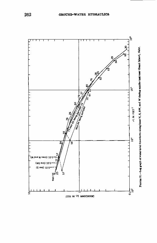
during aquifer test near Grand Island.-._____.___--___-- 26177. Log graph of water-level drawdown along lines N, S, SW, and

W during aquifer test near Grand Island__________-_--_- 26278. Data from aquifer test near Grand Island demonstrating the

effects of a well tapping less than the full thickness of the aquifer_ __ _ ____________-______----__------------- 9RV

CONTENTS V

Page79. Semilog graph of water-level drawdown during aquifer test

near Grand Island___________________________________ 26880. Corrections for drawdowns along the top of an aquifer for

differential fractional parts, A, tapped by the pumped wdl..... ...._____._____.._..__.__________________ 275

81. Corrections for drawdowns along the bottom of an aquifer for different fractional parts, A, tapped by the pumped welL_______________________________________________ 276

82. Graph illustrating the method of correcting drawdowns todetermine T______________________________________ 278

83. Graph showing the distribution of drawdowns near a pumpedwell tapping 40 percent of the thickness of an aquifer. _ _ _ 282

84. Water-level recovery curves for different types of variationof S with time.___________________________________ 284

85. Straight-line plots for cases 1 and 2 and Wenzel's empiricalcorrection applied to case 2-____.-___-_--______-_____- 286

86. Graph showing curves obtained by plotting s' against log(tft1), aquifer test near Grand Island.__________________ 288

87. Straight-line plot for case 1, the uncorrected plot for case 3,and Wenzel's empirical correction applied to case 3______ 290

88. Graph showing curves obtained by plotting s' against log(tit1), aquifer test near Scottsbluff, Nebr_____________ 291

89. Equipment for making a slug-injection test _______________ 30190. Graph showing decline of residual head in a 6-inch well at

Speedway City, Ind., following the instantaneous injection of a 39-gallon slug of water__-_-_____-.___--__-_____-_ 304

91. Map of the Ashland well field of the municipally ownedwater supply of Lincoln, Nebr-_-______-_______-___-___ 312

92. Generalized east-west geologic section through supply well 2in the Ashland well field.._--_____-__--____.__--__-_-_ 313

93. Graphs showing the stage of the Platte River and the waterlevel in observation well 1 in the Ashland well field ______ 314

94. Semilog graph of the average ratio of rising and falling stages of the Platte River plotted against the distance of the ob servation wells from the riveredge.-__--_--__-.--_----- 315

95. Graph of the time lag between maximum and minimum stages of the Platte River and corresponding water levels in observation wells plotted against the distance of the wells from the riveredge---_--_-------------___---_-_- 317

96. Graph showing the drawdown in an observation well 2,000feet from a well pumped at a cyclically varying rate____. 322

97. Hydrograph for a cyclically pumped well showing the sym bolism used for time factors__.____-______-__-_____-_ 325

98. Semilog plot of the factor s-T/264<? against the number ofpumping cycles n for selected values of p___-_-_-__--__- 327

99. Diagram for estimating the transmissibility of an aquiferfrom the specific capacity of a well______--_--___.-_-_ 334

100. Graph showing relation of well diameter, specific capacity,and coefficients of traosmissibility and storage_________ 339

VI CONTENTS

TABLES

Page TABLE 1. Data for aquifer test near Wichita, Kans., giving drawdowns

after 18 days of continuous pumping at 1,000 gpm_________ 2522. Data for aquifer test near Grand Island, Nebr., giving draw

downs after 48 hours of continuous pumping at 540 gpm_ ... 2563. Coefficients of transmissibility and storage determined from the

corrected drawdowns after 48 hours of continuous pumping at 540 gpm during aquifer test near Grand Island, Nebr____ 258

4. Data used in determining the coefficient of permeability from radial components of the hydraulic gradient after 48 hours of continuous pumping at 540 gpm during aquifer test near Grand Island, Nebr--_-__--_-_______________ 264

5. Interruptions in the pumping from well 84 near Grand IslandI' _ i"

Nebr., and the corresponding values of the factor ^ {

used in correcting the 48-hour drawdowns______________ 2706. Data for determination of drawdown at the point of stagnation

beneath a well tapping less than the full thickness of an aquifer_____..____.-._-____________-___ 281

7. Data for a slug-injection test at Speedway City, Ind_________ 3038. Ratio of the range in water-level fluctuation in observation

wells 1, 2, and 3 to the corresponding range in stage of the Platte River at the U.S. Highway 6 bridge. _________ 311

9. Time lag between the minimum and maximum stages of the Platte River at the U.S. Highway 6 bridge and the corre sponding minimum and maximum water levels in observa tion wells 1, 2, and 3__________________________-----_-_ 316

10. Summary of determinations of the coefficient of transmissi bility by the stage-ratio and the time-lag methods.________ 318

GROUND-WATER HYDRAULICS

METHODS OF DETERMINING PERMEABILITY, TRANSMISSIBILITY, AND DRAWDOWN

Compiled by RAT BENTALL

INTRODUCTION

The development of the nonequilibrium formula by Theis (1935) was a major advance in the field of ground-water hydraulics, and Wenzel (1937, 1942) did much to make the formula a practical tool for the hydrologist. Subsequently, general modifications or adjust ments that are applicable to the earlier methods were advocated by Theis and other workers and new formulas for the solution of special field problems also were developed. These papers include suggested corrections for drawdown measurements analyzed by the Theis graphi cal method; remarks pertaining to Wenzel's limiting formula, gradient formula, and the recovery method; a formula for corrections to be applied if wells used for aquifer tests tap less than the full thickness of the aquifer; formulas for the determination of aquifer constants from water level data obtained when a well is bailed or a slug of water is injected into a well; analyses of the effects of cyclic fluctua tions of the water-level, the pumping rate, or the pumping interval; and formulas and a chart relating the specific capacity of a well to the coefficient of transmissibility of the aquifer tapped by the well.

In writing these papers, it has been assumed that the reader under stands the basic definitions relating to ground-water hydraulics and is acquainted with the fundamental nonequilibrium and equilibrium formulas for determining the hydraulic constants of an aquifer. The symbols used, unless otherwise specified, are defined as follows: &=the height of the column of water in the pumped well or in an observation

well anywhere within the area of water-level drawdown, measured fromthe bottom of the aquifer;

m=the thickness of the aquifer; r=the radius of the pumped well or the distance from the pumped well to the

observation well or point at which the drawdown is desired; «=the water-level drawdown in the pumped well, in an observation well, or at

some point in the vicinity of the pumped well; f=the time since pumping began;

243

244 GROUND-WATER HYDRAULICS

t'=the time since pumping stopped;

P=the coefficient of permeability of the aquifer ; p=the rate of discharge from the pumped well ; /Sf=the coefficient of storage of the aquifer ; and T=the coefficient of transmissibility of the aquifer.Also, the terms "semilog" and "log" are used in reference to graphs to mean semilogarithmic and logarithmic, and the units gallons per day and gallons per minute are abbreviated to gpd and gpm, respectively. Furthermore, the aquifer, unless otherwise specified, is assumed to conform to the idealized conditions postulated by Theis (1935, p. 521) .

DETERMINING THE PERMEABILITY OF WATER-TABLEAQUIFERS

By C. E. JACOB

ABSTRACT

If the Theis graphical method is used for determining the hydraulic constants of an aquifer under water-table conditions, the observed drawdowns should be corrected for the decrease in saturated thickness. This is especially true if the drawdown is a large fraction of the original saturated thickness, for then the computed coefficient of permeability is highly inaccurate if based on observed, rather than corrected, water levels.

Wenzel's limiting formula, a modification of the Theis graphical method, is useful where u=r*8/4Tt is less than about 0.01. However, a shorter procedure for determination of the coeflacient of transmissibility, as well as the coeflacient of storage, consists of plotting the values of the corrected drawdowns against the values of the logarithm of r.

Wenzel (1942) suggested that observation wells be situated on lines that ex tend upgradient and downgradient from the pumped well. However, a detailed analysis of aquifer-test results indicates that such a restriction is unnecessary.

The gradient method for determining permeability should yield the same results as the Thiem method. The former, when applied for a distance within the range of applicability of the latter, is merely a duplication of effort or, at best, a crude check. Because of the limitations of accuracy in plotting, the gradient method is much less satisfactory. That Wenzel (1942) obtained iden tical results from the two methods is regarded as a coincidence.

Failure to take into consideration the fact that the pumped well does not tap the full thickness of the aquifer leads to an apparent coeflacient of permeability that is much too low, especially if the aquifer consists of stratified sediments. The average coeflacient of permeability computed from uncorrected drawdowns may be only a little more than half of the true value.

THE THEORY OF PERMEABILITY

Formulas for the steady radial flow of water toward a well that taps the full thickness of an unconfined sand are based upon the premise, originally ^et forth by Dupuit (1863), that for low water-table gradi ents the average of the horizontal, or radial, velocity in a vertical section is proportional to the slope of the water table (6h/6r) that is

v=-k(dh/6r).

The horizontal component of velocity at the water table actually is equal to &(dA/dr)/[l + (dA/dr) 2 ] but, for slopes that are very small in comparison to unity, the (dh/6r) 2 in the denominator becomes in significant. If the small vertical components are neglected, all flow lines in a given vertical plane through the well can be assumed to be

245


both parallel and horizontal ; consequently, the distribution of vertical pressure is hydrostatic or, in other words, the head in a vertical sec tion is uniform. Therefore, the horizontal component of the velocity in a vertical section is also uniform and equals the horizontal com ponent at the free surface, or water table. The time rate of flow per unit width normal to the flow is then Jch (6h/dr) .

In the immediate vicinity of a pumped well that taps the full thick ness of an unconfined aquifer, the slope of the water table is steep and the foregoing relations obviously do not pertain. At distances where the flow toward the well has not yet become steady, the water table is declining at radially differential rates that is, the slope of the water table is changing with time and again the above relations do not pertain. When applying the theory of Dupuit, these limit ing distances should be approximated.

Between the two limits, Dupuit's assumption is valid. Inasmuch as the flow is steady, the inward flow of water through a cylindrical surface concentric with the well equals the discharge of the well, or

(1)

Separating the variables and integrating between TI and r2, which are both within the limiting distances,

Al-A?=(<2M)loge(r2/rO (2)

If one integration limit is considered to be fixed and the other moving, this equation defines, to a sufficient approximation, the lowered water table in the annular area, concentric with the well, over which Du puit's assumption is valid.

Solving equation 2 for k gives

7._ K~

An equivalent expression was first used by Thiem about 1906 to de termine the permeability of an aquifer from drawdowns in two ob servation wells near a pumped well (Wenzel, 1936). Principally through the work of Wenzel, this equation has had widespread appli cation in this country. To minimize errors of observation as well as errors arising from inhomogeneities of structure, Wenzel has advo cated using many observation wells spaced systematically on lines radiating from the pumped well, preferably in upgradient and downgradient directions; then from a modification of Thiem's equation known as the limiting formula, an effective average permeability is determined graphically from drawdowns observed at several points

PERMEABILITY, TRANSMISSIBILITY, AND DRAWDOWN 247

on the two opposing radii. The same result might be obtained more directly, however, by plotting values of h2 against Iog10r. If the equation is a valid engineering approximation, the graph should yield a straight line and the value of k can be determined from the slope of the straight line and Q.

Often the results of an aquifer test are desired in terms of the coefficient of transmissibility (T) of the water-bearing material. The coefficient of transmissibility is the product of &, which can be deter mined graphically from Thiem's relation or from Wenzel's limiting formula and the original saturated thickness, m, which is assumed to be uniform when the water table is in its undisturbed position. A graph of the values of the drawdown, corrected as indicated in the fol lowing pages, plotted against corresponding values of Iogi0r gives T directly, again by the straight-line method. A graph of this kind per mits visualization of the distribution of drawdown and of the ap proximate limits of usefulness of the related linear mathematical expression. Moreover, it is useful in comparing methods involving steady-state drawdowns with those involving nonsteady-state draw downs and in justifying application of the theory of nonsteady flow in a confined aquifer of uniform transmissibility to water-table aquifers wherein the thickness of saturated material diminishes appreciably. In fact, as will be seen in the following pages, only after such correc tions have been made can the graphical procedure of Theis reasonably be applied to nonsteady-state drawdowns.

THEIS GRAPHICAL SOLUTION USING CORRECTED DRAWDOWNS

From equation 3 above,

2.30Qlog10 (r2/r1 )

Substituting s=m h in this relation gives

T= 2.30Qlog10 (r2/r1 )

orT= 2.30Qlog10 (r2/r1 ) (4)

where s sP/Zm is the corrected drawdown.


If the corrected drawdown is replaced by

s'=s-(s2/2m)=m-(h+s2/2m), (5) wheres f is the drawdown that would occur in an equivalent confined aquifer, then

Equation 6 is an expression in terms of the drawdown, s', for the co efficient of transmissibility of a confined aquifer of uniform thickness. To solve equation 6, and hence equation 4, graphically, plot values of s f against corresponding values of Iog10r- and find the slope of the straight-line plot. If As' =s( s'2 is taken as the change in drawdown over one log cycle, then \ogi0 (r2/r1 )=l. and

The nonsteady flow of water toward a well that taps the full sat urated thickness and that discharges at a constant rate from an ex tensive aquifer of constant transmissibility obeys the relation

fJo(8)

where S is in the coefficient of storage (Jacob, 1940, p. 579) . When the time rate of change of drawdown (6s/6t) becomes small in relation to its rate of change with distance, equation 8 reduces to equation 1, which applies to steady radial flow. The integration of equation 8 yields

, 4H-T' where

-2^!+'"} (9)

u=4Tt

For small values of u (that is, when r is small or t is large), equation 9 can be approximated by


When t is constant, this is the equation for the straight line (on semilogarithmic coordinates) in equation 6. After T is determined from the slope of the straight line, S can be determined from the intercept, rei on the r-axis (or the log r-axis). At that point s=0 ; hence

^" _ ., 0.5772_ A tiRO TjU~ e U.OOJ,

from which

5=4-0.562 ^.

Wenzel designated equation 9 as the nonequilibrium formula. It is a particular solution of the general second-order differential equation and is but one of a great many particular solutions for different limit ing conditions. The given limiting conditions are that the discharge of the well is constant, that the initial drawdown (referred to the undisturbed piezometric surface) is everywhere zero, and that the flow across the upper and lower bounding planes of the aquifer is every where negligible.

Equation 9 is a valid engineering approximation of the actual flow only where T is virtually constant. This condition is satisfied in a confined homogeneous bed of approximately uniform thickness or in an unconfined homogeneous bed wherein the drawdowns are small compared to the initial thickness of saturated material. The nonequilibrium method, or graphical procedure of solving the exponential- integral relation for T and S from observations of the variation of s with t or with r, was devised by Theis (Jacob, 1940, p. 582).

When the drawdown is a large fraction of the initial saturated thick ness, the need for correcting the drawdown before applying the nonequilibrium method can be demonstrated by using data from an aquifer test conducted by S. W. Lohman near Wichita, Kans. (Wenzel, 1942, p. 142). Both the observed and corresponding corrected drawdowns in 6 wells after 18 days of continuous pumping at 1,000 gpm, or 1,440,000 gpd, are given in table 1, and both are plotted against r in figure 72 and against r2 in figure 73. The average of the 18-day ob served drawdowns in the corresponding observation wells along the north and south lines gives T 129,000 gpd per foot and £=0.47 by both the straight-line method (fig. 72) and the Theis graphical method (fig. 73), whereas the average of the 18-day corrected drawdowns in the same observation wells gives T= 154,000 gpd per ft and £=0.35 by the same two methods. The average thickness of saturated ma terial at the test site at the beginning of the test was 26.8 feet and after the 18-day period of pumping was 22.3 feet.


133d Nl '(,*) KMAOQAAVaa 031038800 CJNV (') NMOQAAVaCJ Q3Aa3SaO

PERMEABILITY, TRANSMISSIBILITT, AND DRAWDOWN 251

a

133d Nl (,*) NMOQMWKl 031038800 QNV (0 N/IAOOMVMO 03AM3S8O


TABLE 1. Data for aquifer test near Wichita, Kans., giving drawdowns after 18 days of continuous pumping at 1,000 gpm

Well

Distance from

pumped well, r

(ft)

r»

(ft»)

Observed drawdown,

(ft)

«'/2m

(ft)

Corrected drawdown,

(ft)

Ratio of observed to

corrected drawdown

Line extending north from pumped well

1. ..................2... ................3. .._..._. _.._-...._

49.2100.7189.4

2,42010, 14035,900

5.914.583.42

0.65.39.22

5.264. 193.20

1. 121.091.07

Line extending south from pumped well

1. ..................2...................3... -_.--_-__-_.._..

49.0100.4190.0

2,40010, 08036, 100

5. 484.313. 19

0.56.35. 19

4.923.963.00

1. 111.091.06

That the two procedures (the straight-line method and the Theis graphical method) should give identical results for the test near Wichita is clear from figure 73. The approximation for w, upon which the straight-line plotting is based, does not differ by any significant amount from the type curve within the range of values of u that is involved. In this and similar instances, the nonequilibrium method becomes an equilibrium method and the two procedures should check each other within the limits of accuracy of plotting. There fore, in the analysis of aquifer-test data, the straight-line method should be used to determine whether the flow is steady or nonsteady over the range of the distances involved. If the flow is found to be steady, the straight-line method suffices for determination of the hy draulic constants, but if the flow is found to be nonsteady, the Theis graphical method needs to be applied.

Dividing the value of T obtained from the corrected drawdowns by the initial thickness of saturated material, m=26.8 feet, gives k=5,750 gpd per sq ft, which agrees reasonably with Wenzel's P= 5,787 gpd per sq ft. The value $=0.47, which was determined from the uncorrected drawdowns, is believed to be about 0.18 too high because the value $=0.35, obtained from the corrected drawdowns, is only an approximation and becomes even smaller when corrected further for the reduction in saturated thickness. The corrected drawdowns used in determining $=0.35 were those that would have occurred in a con fined aquifer having similar hydrologic properties and a thickness equal to the initial thickness of saturated material in the water-table aquifer. In order to determine the average coefficient of storage more closely, the above determined value may be multiplied by the average


ratio of the final to the initial saturated thickness. The theoretical justification of this procedure follows.

The second-order differential equation governing the radial flow of water in an unconfined aquifer is

//-) (dA/dr)] =S(dfc/dO . (1 la)

Substituting (m s) for h gives

(lib)

which can be expressed in terms of the corrected drawdown, s' rather than the actual drawdown, s, by determining the relationships between their respective differential coefficients. From

dsVdr=[(m-s)/m](ds/dr) (lie)

and

dV/dr»= [(m-s)/m](52s/dr2)- (1/m) (ds/dr)2. (1 1 d)

For low water-table gradient values of (ds/dr) 2 small in comparison with m(52s/^2 ) the last term of equation lid can be omitted and the equation becomes

d2«7dr2 =[(m-s)/m](d2s/dr2). (lie)

The third relation required is

(llf)

Making the substitutions indicated by equations lie, lie, and llf in equation lib gives

which can be rewritten

(llh)

whereT=km

is the initial transmissibility and

S'=[m/(m-s)]S

is the apparent coefficient of storage.

690-185 O 63 2


If the variation of s is small in comparison with m, S' may be con sidered essentially constant, and the integration of equation llh gives equation 9, in which * is replaced by *' and S by S' as one solution. By application of the graphical method of Theis to the corrected drawdowns (*'), the values of T and S' can be determined; the approximate average coefficient of storage is then

S=[(m-s)/m~]JS'. (Hi)

In the test near Wichita, the initial saturated thickness was 26.8 feet; the drawdown averaged over the logarithm of the distance 50 to 200 feet that is, the drawdown at the geometric mean distance, 100 feet was 4.5 feet; and hence S' was found to be 0.35. Therefore,

S= [(26.8-4.5)/26.8]0.35=0.3

instead of 0.47, as determined from the observed drawdowns. This is only an approximate spatial average (at a fixed time) of a coefficient of storage that varies not only with distance from the pumped well but also with time. Even if the coefficient of storage were invariable, its true value could not be determined precisely by this application, to an unconfined aquifer, of the theory of nonsteady flow in an aquifer of uniform transmissibility.

WENZEL'S LIMITING FORMULA

For the aquifer test near Wichita, Kans., Wenzel's limiting formula gives Pf = 5,805 gpd per sq ft, which does not differ significantly from the value obtained by the corrected drawdown methods in figures 72 and 73. The steps involved in the application of Wenzel's limiting formula and in the straight-line method are described below.Wenzel's limiting formula:

1. Tabulate well numbers, distances, and observed drawdowns.2. Plot the water-level data- on graph paper having rectangular coordinates,

and draw smooth curves through the points.3. Determine values of drawdown from these curves for equal but opposite

radii, preferably upgradient and downgradient from the well, and tabulate, for several different pairs of radii, values of B (half the difference in the averages of the upgradient and downgradient draw downs).

4. Determine the average thickness of saturated material upgradient and downgradient between the same pairs of radii, and divide the loga rithm of the corresponding ratios of outer to inner radii by these values. The resulting quotients are values of A..

5. Plot each value of A against the corresponding value of B, draw a straight line through the plotted points and the origin, and from the slope of that line determine Pt (or *).


The straight-line method using corrected drawdowns:1. Tabulate well numbers, distances, and observed drawdowns, and correct

the drawdowns by subtracting (*V2m).2. Plot the corrected drawdowns, *', against r on semilog graph paper, and

draw a straight line through the plotted points; from the slope of that line and from its intercept, determine T and the apparent 8.

Although step 2 in Wenzel's method is not necessary if the observa tion wells are placed in pairs at equal distances upgrudient and downgradient from the pumped well, his method still entails two extra steps that involve considerable computation.

THE LOCATION OF OBSERVATION WELLS

As pointed out previously, Wenzel advocates that lines of observa tion wells be oriented upgradient and downgradient from the pumped well, their location being based upon a preliminary determination of the direction of the natural ground-water flow. Not only his limiting formula but also his applications of the nonequilibrium method make use of such orientation. However, it is questionable whether discrim ination in the choice of direction is warranted.

The equations for unconfined flow are based upon Dupuit's premise, which holds for water-table gradients that, although considered low, are nevertheless steep compared to the usual undisturbed slopes in nature. Whenever an initial natural water-table gradient exists, the distribution of head, or potential, from different sources, natural and artificial, can be added directly by the principle of superposition. This principle is strictly applicable only when the transmissibility is independent of the head that is, when the aquifer is confined. The second-order partial differential equation representing the conditions of artesian flow is linear; hence, the validity of superposing or adding algebraically is verified. For unconfined aquifers, the differential equation is not linear but of the second degree; thus, the superposi tion, for example, of a theoretical radial drawdown distribution on a natural water table having a low gradient gives the approximate re sultant distribution of head only at distances from the pumped well that are greater than a certain limiting distance.

If whatever occurs upgradient is offset by an opposite effect downgradient, averaging the slopes upgradient and downgradient would seem to counteract the nonlinearity for distances close to the well, where Dupuit's assumption also breaks down. This argument presup poses that the superposition of slopes is valid; then, from purely theoretical considerations, there would be no reason for preferring one direction to any other. From a practical viewpoint, both Dupuit's assumption and the principle of superposition seem uniformly valid hi all directions from the pumped well, especially for undisturbed gradients of the magnitude encountered in nature. Even if one


direction were more significant than another, inhomogeneities and variations in the thickness of the aquifer are of greater significance. In fact the location of the observation wells should be based as much, or perhaps more, upon geologic considerations as upon the ground- water gradient. For instance, the configuration of the floor of the aquifer is as important as the configuration of the water table except in the immediate vicinity of the well. Often the geologic structure is not known in sufficient detail to aid in the location of observation wells. Even where the structure is known in detail, seldom does an aquifer meet the specifications regarding uniform initial transmissibility (that is, initial uniform thickness of saturated homogeneous material). Therefore, any advantage that might be postulated by placing the observation wells ungradient and downgradient is gen erally invalidated by the prevailing field conditions.

As an example of the above, consider an analysis of the water level data from an aquifer test near Grand Island, Nebr. (Wenzel, 1936, p. 26-57). As shown in figure 74, the observation wells for this test were drilled along lines radiating from the well which was to be pumped. During the test, pumping was continuous for 48 hours at an average rate of 540 gpm. The data needed for application of the graphical method to the corrected 48-hour drawdowns are given in table 2 and are plotted in figures 75, 76, and 77. Table 3 summarizes the determinations of the coefficients of transmissibility and storage for all lines except $, for which the water-level data were not sufficient for a separate analysis. (Actually, the fact that the pumped well did not tap the full thickness of the aquifer completely upsets the analysis and gives misleading results; this is discussed in a later section of this paper.)

TABLE 2. Data for aquifer test near Grand Island, Nebr., giving drawdowns after 48 hours of continuous pumping at 540 gpm

WellDistance frompumped well,

T(ft)

r*(ft')

Observeddrawdown,

*(ft)

g*!2m(ft)

Correcteddrawdown.»'

(ft)

Line A

1. .-._-_.-.......2-. .-.-.-..... ...3... -------------4---------------5- 6... -------------7.... ......8........ ......9 ~ ..10..-------.----.11. - -------------

24959.9114 41642229354429479604755904

6203,590

13, 09027,00052,400

125, 300184, 000229, 000365, 000570, 000817, 000

4. 012.792.031. 611. 14.65.52.44.26. 16. 11

0.08.04.02.01.01.00.00.00.00.00.00

3. 932. 752.011. 601. 13.65.52. 44.26. 16. 11


TABLE 2. Data for aquifer test near Grand Island, Nebr., giving drawdowns after 48 hours of continuous pumping at 640 gpm Continued

WellDistance from pumped well,

(ft)

r» (ft»)

Observed drawdown,

(ft)(ft)

Corrected drawdown,

(ft)

LlneB

13.... ___________ 29.9 89414.____________ 70.0 4,90015-__-_-- - 120.0 14,40016.._. ___________ 184.9 34,20017_______________ 255 65,00018__............. 375 140,60019.... ___________ 425 180,60020-_____________ 500 250,00021_______________ 650 423,00022___.___________ 775 601,00023...._._._...... 974 949,00024_______________ 1,149 1,320,000

Line W

25..-.----_-----. 49.7 2,47026..._._--.....__ 170.0 28,90027__________.____ 270 72,90028............... 430 184,90029__......_______ 625 391,000SO---..---.------ 805 648,00031_------------ 940 884,000

LineD

32-_-_-_---__---_ 40.1 1,60833______.___ ___ 95.1 9,04034._. ____________ 144.7 20,90035--------.------ 214 45,80036.. _____________ 324 105,00037-----------.--- 423 178,90038..----_-..--._. 448 201,00039-_----_----_-.- 573 328,00040___----_-______ 723 523,00041-.-------.----. 872 760,00042___-____-______ 1,073 1,151,00043....----.-.__-- 1,197 1,433,000

LlneC

44-.-...-......- 39.3 1,54445-----------.- 80.5 6,48046--. ---------- 130.3 16,98047--.--- ------ 195.6 38,30048-.------------ 286 81,80049_.._._._. 410 168,10050____-------- 425 180,60051------ ----.- 535 286,00052__._._... 685 469,00053________ 835 697,00054...._____... 1,035 1,071,00055...____--.. 1,175 1,381,000

3. 872.591. 861. 31

. 92

. 51

.40

.29

. 16

. 10

.05

.05

0.07 .03 .02 .01 .00 .00 .00 .00 .00 .00 .00 .00

3. 802.561.841. 30.92.51. 40.29. 16. 10.05.05

2.981.44

. 84

.45

.21

. 11

.09

0.04 .01 .00 .00 .00 .00 .00

2.941. 43

. 84

.45

.21

. 11

.09

3. 152. 241.711.24.77.51.46.28. 15. 10.06.05

0.05 .03 .01 .01 .00 .00 .00 .00 .00 .00 .00 .00

3. 102.211. 701.23.77. 51. 46. 28. 15. 10.06.05

3.232. 371.72

217841392412080301

0.05 .03 .01 .01 .00 .00 .00 .00 .00 .00 .00 .00

3. 182.341. 711. 20.78. 41.39. 24. 12.08.03.01


TABLE 2. Data for aquifer test near Grand Island, Nebr., giving drawdowns after 48 hours of continuous pumping at 540 gpm Continued

WellDistance frompumped well,

f(ft)

r*(ft*)

Observeddrawdown,

t(ft)

»*frm(ft)

Correcteddrawdown.

if(ft)

UneSW

56_______________57_______________58... ._._..__.___59-------__-_____60____ .__._.___._61____ _ .__. __62.. _..._._._..__63_.___ __________64_________._.___65- ___ ___-.-__66_______ __ ____67_._____________68_______________

46.769.593.6118.0217317417517617717817917

1,017

2,1804,8308,76013,92047,100100,500173,900267,000381,000514,000667,000841,000

1, 034, 000

3. 122.582.181.861. 11.66.41.28.20. 13.09.08.07

0.05.03.02.02.01.00.00.00.00.00.00.00.00

3.072.552. 161 841. 10.66.41.28.20. 13.09.08.07

LlneS

73_______________74_________._____75 ___________ _76_______________

130. 1225280383

16, 93050,60078,400

146, 700

1.731.00.76.55

0.01.01.00.00

1.72.99.76.55

LineN

7778798081

63.2160.0262342446

3,99025,60068,600

117, 000198, 900

2.671.63.96.65.42

0.04.01.00.00.00

2.631. 62.96.65.42

TABLE 3. Coefficients of transmissibility and storage determined from the corrected drawdowns after 48 hours of continuous pumping at 540 gpm during aquifer test near Grand Island, Nebr.

Line

A.___________________B_--.___________.____W-_.______. _________D..__________________C _________________SW.____. ____________N __ ________________

Value of * for W(«)=4.04

(ft)

2.452.782. 502.502.672.752. 50

Value of r* for «=0.01

(ft»)

5,8003,7004,7005,3003,8003,6004,700

Coefficient of transmissibility,

T (gpdperft)

102, 00090, 000

100, 000100, 00094, 00091,000

100, 000

Coefficient of storage, S

0. 19.26.23.20.265.27.23

July

193

1

FIG

URE

74.

Map

show

ing

the

loca

tion

of w

ells

use

d fo

r aqu

ifer

test

nea

r O

rand

Isl

and,

Neb

r.to & C

O


bU *u- <

PERMEABILITY, TRANSMISSIBILTTY, AND DRAWDOWN 261

ITIIIIII

T0'0= n

I I I I I I I

I I I I I I

z »,7- a- s

133d Nl '(*) NAAOQAAVMQ


iaaj NI '(*)

PERMEABILITY, TRANSMISSIBILrTT, AND DRAWDOWN 263

The average coefficient of transmissibility obtained from the data for all lines of wells is T= 97,000 gpd per ft and the average coefficient of storage is £=0.23. For the lines B and D, which extended upgradient and downgradient, respectively, from the pumped well, the averages are T= 95,000 gpd per ft and /S'=j.BC, and for lines A and C, which made a right angle with lines B and D, the averages are T= 98,000 gpd per ft and £=0.23. The results in table 3 show that, in general, where T is small S is large, a fact which probably indicates that the aquifer thickens somewhat toward the north or northwest. Any significance attached to the different average values of T from lines B and D and lines A and C is outweighed by anomalies arising very probably from differences in thickness.

THE GRADIENT FORMULA If equation 1 is solved for &,

and when (dh/dr) -and h vary with the angle 0, then

(13)

Wenzel's equation (Wenzel, 1942, p. 86, eq 82), which is the basis of the so-called gradient method, is obtained through approximation of the integral of equation 13 by averaging the gradient and the satu rated thickness at the distance r upgradient with those at the distance r downgradient. This method should yield results that are equivalent to the results obtained by the Thiem method because both are based on equivalent relations and one is the integral of the other. If the former is applied at a distance within the range of applicability of the latter, the same data being used, the result is in effect a duplication of effort. The gradient method adds nothing to the Thiem method. Moreover, it is much less accurate because of the limitations of accu racy in plotting and drawing smooth curves.

The applicability of the gradient method is illustrated by compu tations from table 4, which is a modification of a corresponding table by Wenzel (1942, p. 124). Values of F/, computed by the gradient formula for r=115 feet and r=125 feet, are

^9,168 ft-min per dayX540 gpm '~ 115 (98.09+97.98) 0.21 ft3 = 1,050 gpd per sq ft;


and

p _9,168 ft-min per dayX 540 gpm ' 125(98.19+98.08)0.21 ft3

=960 gpd per sq ft.

The 9 percent difference in the results of these computations is to be expected inasmuch as the differences in water-level altitude given in table 4 are accurate only to the nearest hundredth of a foot. To indi cate that only 2 figures are significant, both results should be written as 1,000 gpd per sq ft. Moreover, because the slope (0.009) 115 feet downgradient from the well is smaller than the slope (0.010) 125 feet downgradient from the well, the agreement between the value of Pf determined by the gradient method and the one determined by the limiting formula should be regarded as fortuitous.

TABLE 4. Data used in determining the coefficient of permeability from radial components of the hydraulic gradient after J^8 hours of continuous pumping at 540 gpm during aquifer test near Grand Island, Nebr.

Direction from pumped well

Altitude of water table (ft)

110 ft from pumped

well

1,808.44 1,808.06

120 ft from pumped

well

1, 808. 56 1, 808. 15

Difference (ft)

0.12 .09

.21

Altitude of water table (ft)

120 ft from pumped

well

1,808.56 1, 808. 15

130 ft from pumped

well

1, 808. 67 1, 808. 25

Difference(ft)

0.11 .10

.21

WATER-LEVEL CORRECTIONS FOR WELLS TAPPING LESS THAN THE FULL THICKNESS OF AN AQUIFER

If a pumped well does not tap the full thickness of the aquifer, the drawdowns measured in observation wells tapping only the uppermost part of the aquifer should be corrected (Muskat, 1937, p. 368). Be cause of the convergence of the flow lines in the vicinity of the well, the loss of head along the top of the aquifer is greater than the loss of head along the bottom and both differ from the head loss that would occur if the pumped well tapped the full thickness of the aquifer. This is especially true if, as is usually the case, the aquifer consists of stratified sediments. Even homogeneous beds of water- deposited materials are invariably anisotropic. The inhomogeneities of stratification give a resultant permeability in the vertical direction that is many times smaller than the average permeability in the hori zontal direction, producing in a sense an equivalent anisotropy. As a result, the effect of tapping only the upper part of the aquifer is ac centuated; that is, the lateral extent of the disturbing influence is increased.


The effects of a well tapping only the upper part of an aquifer are shown in figure 78, which is based on data from the aquifer test near Grand Island, Nebr. (Wenzel, 1936, 1942). Figure 784 is a section along line SW of observation wells. The pumped well, well 83, was only 40 feet deep and was perforated throughout its length. That the thickness of saturated materials at this site is about 100 feet is shown by the graphic log of well 84 (fig. 78#), which was 25 feet south of well 83. Thus, because the static water level in the well was about 5 feet below the land surface, well 83 effectively tapped only about 35 percent of the full thickness of saturated material.

Figure 78C' shows the streamlines and equipotential lines that would be obtained if the sediments were homogeneous and isotropic. The lines of equal potential, or in this case equal drawdown, were deter mined from Muskat's equation (Muskat, 1937, p. 268, eq. 9). The flow lines were sketched in to form an orthogonal system. In this hypothetical case, the tapping of only the upper part of the aquifer affects the distribution of head for a distance of about 150 feet out from the pumped well. However, because the sediments are stratified, the flow pattern actually is distorted as shown in figure 78A. Lab oratory determinations of the permeability of bailer samples, plotted beside the log of well 84, range from 2 to 4,350 gpd per sq ft. Weighted according to thickness, for flow parallel to the plane of bedding, these permeabilities average 1,200 gpd per sq ft, but weighted according to reciprocal flow lengths, for flow across the plane of bedding, they average only about 150 gpd per sq ft. This suggests an equivalent anisotropy characterized by the permeability ratio (kr/ke ) =8. Ac tually, in order to make the observed drawdowns compatible with the computed drawdown at the point of stagnation underlying the well, this permeability ratio was found to be more nearly twice as large as indicated. In other words, the beds, on the average, are effectively about 16 times as permeable in the horizontal direction as in the vertical direction.

The flow pattern in figure 784 can be obtained by plotting the orthogonal net of figure 78/? on an elastic rectangular sheet which is to be stretched to four times its original length without reducing its width, or the stretching can be performed graphically.

The distribution of drawdown along the top and bottom of the aqui fer is shown in figure 78Z?; a semilog plot of the identical data is shown in figure 79. In both diagrams, the points plotted as open circles repre sent the corrected drawdowns (see table 2) for wells 56 to 68 for the time when well 83 had been pumped continuously for 48 hours at 540 gpm. Because none of the observation wells extended more than a few feet below the water table, the facts that the pumped well tapped only 35 percent of the full thickness of the aquifer and that the effective


12

i33j NI 'saruirw

<Pu

m we

1

3 =7

80.0

00 g

pd.

tt =

l pe

d II

56

57

58

59

T =

180

.000

gpd

per

ft.

m =

80

Virt

ual

100

« ex

tern

.)

61

42

63

64

65

bou|I

Mto

r» M

i i

i i

i i

i i

!i*>

H1

11 1

1 1

cJ

fel

fel

hi

-J!i

i i

i i i i r

i

j i

i

fel

inl

4_0| # C

1 1

| |

, 1

1

1 fc 1 1,

1 IN N

1

0_

0

i i i ,

i i

l~

1jo

j

! 1

1 V

1 1

1

67

68

5 i i

i40

0 50

0 60

0 RA

DIAL

DIS

TAN

CE

(r),

IN

FEET

D

700

re=

775

*00

Q =

780,

000

gpd.

a =

0.7

0, k

r/k

z =

16,

J-

180,

000

gpd

per

ft,m

= 1

00 f

t W

ell

84

' ^

-i

56

57

58

59

60

61

6266

4000

20

00

0

k, G

PO P

ER F

T 2

400

500

600

RADI

AL D

ISTA

NC

E (r

), I

N FE

ET

E

too

FIOU

HE 7

8. D

ata

from

aqu

ifer

tes

t ne

ar G

rand

Isl

and,

Neb

r., d

emon

stra

ting

the

effe

cts

of a

wel

l ta

ppin

g le

ss t

han

the

full

thic

knes

s of

the

aqui

fer.

A,

Sect

ion

alon

g lin

e 8 W

sho

win

g id

ealiz

ed in

flue

nce

of w

ell 8

3, w

hich

ext

ends

35

feet

into

a s

uppo

sedl

y ho

mog

eneo

us a

niso

trop

ic w

ater

-tab

le a

quif

er 1

00 fe

et t

hick

. B

, D

istr

ibut

ion

of d

raw

dow

n as

obs

erve

d al

ong

the

top

and

as i

nfer

red

alon

g th

e bo

ttom

of a

wat

er-t

able

aqu

ifer

100

fee

t th

ick

if th

e pu

mpe

d w

ell e

xten

ds 3

5 fe

et in

to th

e aq

uife

r;

also

the

dist

ribu

tion

of d

raw

dow

n th

roug

hout

a w

ater

-tab

le a

quif

er 1

00 fe

et th

ick

if th

e pu

mpe

d w

ell e

xten

ds to

the

botto

m o

f the

aqu

ifer

. C,

Str

eam

lines

and

equ

i-

pote

ntia

ls f

or a

pum

ped

wel

l tha

t ext

ends

35

feet

into

an

isot

ropi

c w

ater

-tab

le a

quif

er 1

00 fe

et t

hick

; al

so th

e ap

prox

imat

e di

stri

butio

n of

dra

wdo

wn

alon

g th

e fa

ce o

f th

e w

ell a

nd a

long

dow

nwar

d ex

tens

ion

of w

ell a

xis.

D, H

ypot

hetic

al fl

ow p

atte

rn fo

r pur

ely

radi

al fl

ow in

duce

d by

a w

ell e

xten

ding

to th

e bo

ttom

of a

n eq

uiva

lent

ar

tesi

an a

quif

er.

E, A

ppro

xim

ate

patte

rn o

f flo

w in

sec

tion

alon

g lin

e SW

pro

duce

d by

wel

l 84,

whi

ch h

as tw

o le

ngth

s of

per

fora

ted

casi

ng; a

lso

the

vert

ical

var

iatio

n of

per

mea

bilit

y as

det

erm

ined

in t

he la

bora

tory

and

col

umna

r sec

tion

base

d on

log

of w

ell 8

4.

to

CORRECTED DRAWDOWN (s')T> Ui *i

_

-

-

K\

\\>

* o o \ Q.IT <T \<. y. ?s X f A ?A \

-2-S ;.< \£| go. X

A 3 o 01Q-S 2.$ (6"°- <" a

-» 3 5 3

:l| |f 5

\

\

\

\_i Q.

O

o"

OQ

O 13

V 2,

ViX

AFTER 48 HOURS OF PUMPING, IN FEETw r\> _ o

L

^

"

V

ftn-zS. »S. r"I? 5° z IT i

SS g-a > , t« c = » n <r

QJ-O -,. Q) Z _

N 5roK) $. ^

^ S "A C A in ., .eg 2. »

? $ ^

°w oo ^Q.CJ

_

1 90 1

r\> o. hoK) "2 * un 5 "2

^ So

^ '1 _i_

§ho 71 *» p

x S* K) 0 ^.

11 " ^" -o = ° P x QO > (6

2.2 oo * " * Q. _ W*<

(k> O

11a. a.? f

o 133T C

||

\ oT2.

\lf \ » a

\lI

\

Vvl X

__ Ny

go

K)

X^J

oo

§

FQ3a.

1

(Q0>

+ <aH 5 2- -5

5'

O

13ta

I

|oS v v

\\\

0

"o

K)

3,

3

)

+

K' ^ 1 \. V^^0^u"\\

N^2^L

Aa»\

t'*T

_

-

-

-

-

"

_

-

-

_

-

-

-775'=rel

v ~\ 1"

M24mVk^=1600 ft 1*


permeability ratio of the aquifer was 16 were taken into consideration when the drawdowns along the bottom of the aquifer were computed.

As mentioned above, the drawdowns along the bottom of the aquifer, as determined from those observed along the top, must be compatible with the drawdown at the point of stagnation, which theoretically is independent of the degree of anisotropy. The drawdown at this point was determined by Muskat's method. The head at the stagnation point should be approximately 2.17 (Q/Zn-T) lower than the head at a distance equal to four times the thickness of an equivalent isotropic sand (or 16 times the thickness of the actual sand). The drawdowns for a well tapping the full thickness of the aquifer, indicated by a dashed straight line in figure 79, were also computed from Muskat's equation. The drawdown on this curve at r= 1,600 feet is 0.49 foot. Thus, the drawdown at the stagnation point probably is about 1.0 foot (see figs. 78Z? and 79).

The foregoing analysis of the effects of pumping from a well that taps only the upper part of an aquifer is based upon a theory that, strictly speaking, is applicable only to confined, or artesian, aquifers. However, it gives an approximation of the actual conditions in an unconfined aquifer that is close enough for the present discussion.

The uniform logarithmic drawdown distribution for steady flow toward a well that taps the full thickness of an equivalent artesian aquifer is shown in figure 78Z> by dashed lines representing traces of concentric cylindrical surfaces in the vertical plane. The distribution is approximately logarithmic out to a distance of about 400 feet. The nonsteady drawdowns at greater distances are represented by the solid vertical lines.

From the slope of the dashed straight line in figure 79, the coefficient of transmissibility is found to be about 184,000 gpd per foot. From corrected drawdowns, Wenzel (1942, p. 147) computed the permeabil ity to be about 1,000 gpd per sq ft, which is equivalent to a transmis sibility of 100,000 gpd per foot. Hence, for this aquifer test, failure to take into consideration the fact that the pumped well tapped only the upper part of the aquifer resulted in an apparent transmissibility that is only 55 percent of the probable true value.

The straight line in figure 79 intersects the zero-drawdown line at r=775 feet, the apparent external radius of the system after 48 hours of continuous pumping. The coefficient of storage determined from this is 0.18, whereas Wenzel obtained 0.217.

The above evaluation of the aquifer test made by pumping from well 83 is confirmed by comparing that test with the test made by pumping from well 84. Well 84 was 105 feet deep, and because the top 24 feet and the bottom 48 feet of the casing were perforated it effectively

690-185 O 63 3


tapped about 70 percent of the full thickness of the aquifer (see fig. ?8ff). This well was pumped intermittently for 2 days at about the same rate as well 83, or 540 gpm. Because of the interruptions in pumping and the uncertainties involved in correcting for them, com putations for this test were not published, although drawdown curves for three observation wells were given by Wenzel (1936, pi. 5).

A reasonable correction for the interruptions can be made by assum ing that the coefficient of storage remained constant. Then, if t' is the time interval back to a given shutdown and t" is the time back to the beginning of the pumping interval, the corresponding correction to be applied to the 48-hour drawdowns is

log, (t'lt") =

and the total correction is

log,

Corrections for the interruptions in pumping are given in table 5. Because successive interruptions of short duration have been lumped together, the computed correction is a liberal one :

778,000 gpdXO. 166 = ' A°f; -j j- 4xX 184,000 gpd per ft

. , . =0.056 foot.

TABLE 5. Interruptions in the pumping from well 84 near Grand Island, Nebr., and the corresponding values of the factor (t'-t")lt" used in correcting the 48- hour drawdowns

[Pumping began at 8:05 a.m. on Sept. 9,1931; average pumping rate was 540 gpm]

Period of interruption

Pumpingstopped

Septem

11:18 a.m.....12:35 p.m __ .2:00 . 5:55 ..

Septemb

4:26a.m.__-8:57- 9:36-.. .9:39 . 9:48 .

11:17 . ..11:49 . 12:06 p.m ___

Pumpingstarted

er 9, 19S1

11:35 a.m.... .12:37 p.m .....3:38- - 6:31...-

er 10, 19S1

6:03 a.m __ .9:32. 9:38-.. 9:40 9:51.

11:19... 11:55. 12:11 p.m.....

t'

Hours

44434238

2723222222202019

Minutes

4730

510

39

292617481659

t"

Hours

44434037

26OO

222222202019

Minutes

30282734

23327OK

14461054

t'-t"

Hours

0010

10000000

Minutes

172

3836

3735213265

t'-t"t"

0.006.001.040.016

.062

.026

.001

.001

.002

.002

.005

.004

2-0. 166


The corrected drawdowns in the three wells are as follows:

Well 57._-----___.__.feet._ 2.16+0.06=2.2259___.___________do_- 1.45+ .06=1.5161_.-.__.-_______do-- .58+ .06= .64

These points are plotted in figures 78Z? and 79. Because the two perforated lengths of casing in well 84 are at the top and bottom of the sand, Muskat's theory, which assumes a single length of perforated casing at either the top or bottom, does not apply. However, the draw downs observed when well 84 was pumped were much less than the drawdowns at corresponding distances when well 83 was pumped. Hence, the effect of tapping different fractional parts of the full thick ness of an aquifer is clearly demonstrated.

CORRECTION OF DRAWDOWNS CAUSED BY A PUMPED WELL TAPPING LESS THAN THE FULL THICKNESS OF AN AQUIFER

By C. E. JACOBABSTRACT

If a pumped well taps less than the full thickness of a confined aquifer, it is less efficient than it would be if it were to tap the full thickness. Also, the distribution of head in its vicinity differs from that which would characterize a well having the same effective radius, discharging at the same rate, but tapping the full thickness of the aquifer at the same location. Because the formulas for deter mining the hydraulic constants of an aquifer are based on the assumption that the pumped well taps the full thickness, the observed water-level drawdowns caused by pumping from a well which taps less than the full thickness should be corrected before they are used in the formulas. Muskat (1932) and Kozeny (1933) described the problem in detail, and Wenzel (1942) gave it cursory treatment. This paper not only outlines the method of making the corrections, but also includes the necessary graphs. It also includes a table for determining the drawdown at the point of stagnation beneath a pumped well that taps less than the full thickness of an aquifer.

THE FORMULA FOB CORRECTING DRAWDOWNS

Whether or not a pumped well taps the full thickness of an aquifer is of practical significance. Not only is the productivity of the well affected but also the distribution of head in its vicinity. If a well that is pumped in making an aquifer test taps less than the full thick ness, the water-level drawdowns observed during the test must be cor rected before an accurate coefficient of transmissibility, or of perme ability, can be computed. The corrections are necessary because the formulas for the determination of hydraulic constants from aquifer- test data are based on the assumption that the pumped well taps the full thickness.

Muskat (1932, p. 329-364; 1937, p. 263-286) developed an equation for the discharge of a well that taps only a fraction of the full thick ness of an aquifer in terms of the full thickness and permeability of the aquifer, the fractional part tapped by the well, and the total potential drop from the assumed effective external radius of the system to the known internal radius. Kozeny (1933, p. 101) summarized Muskat's analysis by a somewhat simpler empirical expression that is a sufficient approximation for many purposes. Kozeny's empirical formula can be written

2irTsv,a[l+7(rj2am)* cos Qra/2)] m V- loge (iv/r.) * '

orQ=Qoa[l+7(rv,/2am)* cos ftra/2) ]=&«/#, (2)

272


where

l/Cr=l+7(rw/2am)» cos ( /2). (3)

In these equations

Q=ihe rate at which water is discharged by a pumped well thattaps less than the full thickness of the aquifer,

Q0 =ihe rate at which water would have been discharged if thewell had tapped the full thickness of the aquifer,

T=the coefficient of transmissibility of the aquifer, m=the full thickness of the aquifer, a=the fractional part of m tapped by the pumped well,

rw =the radius of the pumped well, Su,=the drawdown in the pumped well (that is, the drawdown at

distance rw). re =the external radius of the system (that is, the distance from

the pumped well to the locus of zero drawdown), and (7= the correction factor.

The apparent transmissibility, 7", referred to the total thickness of the aquifer and determined from observations of the drawdown in a pumped well, is given by

y/ =Q log. WO. (4) 2ir«u,

Similarly, the true transmissibility is

Hence,

f-Kwhich is the ratio of the true to the apparent transmissibility, or of the true to the apparent permeability. From equation 6,

(7)

which is the correction factor given by Wenzel (1942, p. 109), This correction is only for values of permeability or transmissibility de termined from the drawdown inside the pumped well. Moreover, as $o is unknown, equation 7 does not lead to a solution of the problem ; however, Q0 can be determined from equation 2.


Muskat (1937, p. 283) states that the flow of water toward a pumped well that taps only a fractional part of an aquifer becomes almost exactly radial at a distance from the well equal to twice the aquifer thickness. However, this is true of isotropic aquifers only, and most aquifers that consist of water-deposited sediments are stratified and, therefore, as a whole, are anisotropic. The flow toward a well that taps less than the full thickness of an anisotropic aquifer becomes radial at a distance from the well equal to twice the aquifer thickness multiplied by the square root of the ratio of the horizontal to the vertical permeability. For example, if an aquifer is 16 times as permeable in the horizontal as in the vertical direction, then purely radial flow occurs only beyond a distance equal to about 8 times the aquifer thickness. Drawdowns measured within the area in which flow toward the well is radial must be corrected if the coefficient of transmissibility computed from them is to be accurate.

In order to correct the drawdowns, the distribution of head through out the aquifer must be known. However, because the foregoing equations relate merely to the difference in head between the inflow and outflow surfaces, they are inappropriate for use in determining the distribution of head in the vicinity of a pumped well. Instead, the distribution of head may be found from two equations derived by Muskat (1937, p. 268, eq. 8 and 9) one for small values of r and the other for large values of r. The latter contains one term for the logarithmic distribution of head for purely radial flow and a second term for the difference between the actual distribution and the loga rithmic distribution. For convenience, consideration need be given only to the distribution of head as found from drawdowns measured along the top and along the bottom of the aquifer; such drawdown readings are found from one series of observation wells or piezometers that extend into the uppermost port of the aquifer only and from a second series that extend to and are open only in the bottommost part of the aquifer. The divergence of the head from a purely logarithmic distribution at a distance r from the well is given by

(2/«r) Zf I(± l)*Ko(n*r/m) sin (mm)] =8, (8)

n

where K0 stands for the modified Bessel function of the second kind of zero order, the plus sign is for the drawdown distribution along the top of the aquifer, the minus sign is for the distribution along the bottom of the aquifer, and 8 is the drawdown correction factor.

Figures 80 and 81 are based on data computed from equation 8 and give, for different fractions of aquifer tapped by the pumped well, the


10- *

FIOUBB 80. Corrections for drawdowns along the top of an aquifer for different fractional parts, a, tappedby the pumped well.

correction factor to be applied, respectively, to drawdowns measured along the top and the bottom of the aquifer.

From equation 8A»=8«?/3»r), (9)

where A* is the drawdown correction the difference between the observed drawdown and the drawdown that would have resulted if the pumped well, discharging water at the same rate, had tapped the full thickness of the aquifer.


10

FIGUXI 81. Corrections for drawdowns along tne bottom of an aquifer for different fractional parts, a,tapped by the pumped well.

If the well is assumed to tap only the upper part of the aquifer, the drawdown will be greatest along the top of the aquifer and least along the bottom because of the convergence of the streamlines upon the opening to the well. If the well is open to only the bottom part of the aquifer and no part of the aquifer is unwatered, the drawdown pattern is similar, though inverted, to that for the well open only to the top part of the aquifer. The curves in figures 80 and 81 do not apply if the screen is in some intermediate position, nor clo they apply, strictly speaking, to unconfined aquifers.

PERMEABILITY, TBANSMISSIBILITY, AND DRAWDOWN 277

APPLICATION OF THE FORMULA

Application of the formula for correction of drawdowns caused by a pumped well that taps only the upper part or only the lower part of an aquifer and the procedure for determining the coefficient of transmissibility of an aquifer from the corrected drawdowns are best illustrated by an example. Assume that a well having -an effective radius of 1.0 foot and its screen set in the top 40 feet of an artesian aquifer 100 feet thick (hence, a =0.40) has been pumped at a constant rate of 840,000 gpd long enough to establish steady radial flow beyond the most distant of 3 observation wells. The drawdowns in the obser vation wells, which tap only the top of the bed and which are 50, 100, and 150 feet from the pumped well, are 5.02, 3.18, and 2.30 feet, respectively. The drawdown in the pumped well is 18.4 feet. If the screen loss is negligible and the aquifer is homogeneous and isotropic with respect to permeability, determine the coefficient of transmissi bility of the aquifer from observed drawdowns.

First, plot the drawdowns against the logarithm of their respective distances from the pumped well (see fig. 82). Draw a straight line (line I) as closely as possible through the plotted points and make a preliminary determination of the coefficient of transmissibility from the formula

where As = the drawdown difference over one log cycle. From figure 79 and equation 10

, 2.30X840,000 __ __ T= 2^(9.1-3.2) as58 '00

and, hence,

_fi___Af__6.9_ 2xr~2.30~2.30~2 '

Assume, as a first approximation, that the above value of T is correct and make the following computations and corrections from the given data and figure 80:

Wettl WeUt WeUS Distance, r,_ _ _ _ . __ _ ___ ._ ______ . _ __.feet__ 50 100 150*r/m=7rr/100_ _...__. _ _____________ __ ________ _ _ 1.57 3.14 4.71Observed «« ____ _ _______ _ _______ _ ____ feet__ 5.02 3.18 2.30«, from figure 80___. ____ __ __ _______________ 0.31 0.045 0.008As tov, from equation 9______ _ __ __ __ __ __ ___feet__ 0.80 0.12 0.02Corrected drawdown =s As_____ ___ __ ____ _ _ do__ 4.22 3.06 -2.28

to

0̂0 o

a

o

10

100

DIS

TAN

CE

(r

), I

N

FEE

T4m

1000

FIG

URE

82.

Gra

ph il

lust

ratin

g th

e m

etho

d of

cor

rect

ing

draw

dow

ns to

det

erm

ine

T.


Plot the corrected drawdowns against their respective values of r, and draw a straight line through the points (line II) (see fig. 82). Make a second trial determination of T and Q/%irT:

2.30X840,000 __ n _ _ , ^ 2^(7.1-3.1) => gpd per '

and

P, _ _ -. == _ _ -.- 1. /4 It.2-n-T 2.30 2.30

Further correct the observed drawdowns by repeating the above pro cedure using the corrected values of T and

Wett 1 Wett t Wett SObserved s tav,. ------------------------------- feet.. 5.02 3.18 2.30«, from figure 80 _______ _ _______ _ ___________ _ _ 0.31 0.045 0.008As, op, from equation 9-. _ ________________ ___.-feet-_ 0.54 0.08 0.01Corrected drawdown = s As_---__-_-___------__do--- 4.48 3.10 2.29

Again, plot the new values of corrected drawdowns and draw a straight line through the points (line III) (see fig. 82). Make a third trial determination of T and Q/%irT:

andQ As 4.5

Repeating the procedure a fourth time results in line IV (fig. 82), from which T = 69,000 gpd per ft and Q/%*T= 1.94 feet. These prob ably are close enough to the true value, and further computations are not necessary.

As a further check, however, the drawdown that would occur in a pumped well tapping the full thickness of the aquifer can be deter mined from equation 1. Solving this equation for the hypothetical drawdown, (Q/2irT)loge (re/rw), yields s^afC, where C is defined in equation 3. In the above example,

1 , . 7 cos (0.2ir) , . 7 (cos 0.628) _ _ . C=l+ V80 =1+ 8.94 =Lb34'

and, therefore,

^£=18.4X0.40X1.634=12.0 feet,

which is identical to the s-ordinate of the point of intersection of line IV with the line r-rw =l foot in figure 82. This indicates that the corrected drawdowns represented by line IV are the drawdowns which would result if a well tapping the full thickness of the aquifer dis-


charged 840,000 gpd and that the coefficient of transmissibility of the aquifer is T= 69,000 gpd per ft.

The lower dashed line in figure 82 gives the probable distribution of drawdown as measured in wells that are open to only the top part of the aquifer. The drawdowns that would have been observed in wells 1,2, and 3 had they extended to and been open to only the bottom part of the aquifer can be determined by making a correction using figure 81:

Corrected drawdown, from line IV, figure 82_ _feet_ _ 5, from figure 81 ______________________________Asbottom, from equation 9____--___-_------_feet-_

Well 1 Well I Well 3

4. 42 3. 09 2. 28-0. 28 -0. 044 -0. 008-0.54 -0.09 -0.01

3. 88 3. 00 2. 27

The upper dashed line through the bottom points in figure 82 gives the probable distribution of drawdowns as measured along the bottom of the aquifer.

DETERMINATION OF THE DRAWDOWN AT THE POINT OPSTAGNATION

If the distribution of drawdown in the vicinity of a well that taps only the upper part of an aquifer is to be represented graphically, the drawdown at the point of stagnation beneath the well must be deter mined. In table 6 the difference between the drawdown, s0 , at the point of stagnation and the drawdown, s4m < at a distance of 4m, is given in units of (Q/2irT) for different values of a under two alternative assumptions regarding conditions at the well face. The data in the second column were computed from an equation derived by Muskat

TABLE 6. Data for determination of drawdown at the point of stagnation beneath a well tapping less than -the full thickness of an aquifer

Fractional part of aquifer tapped by pumped well

o.oo__. ________________________________________0.05 _____________________________________ .-.0.10_. __________________________________ _______0.20_______ ____________ _____________________0.25 ____________________________ ____________0.30_._. _______________________________________0.40._-_- _ .- _____0.50... _________ _____0.60__. ----__-..-_______.___.__.___.__.____-_._0.70_-_-_._.___ _____0.75 _______________ ______ __________0.80__________._ _ _____0.90.__________________ ___ _ _ _________

(*0-*4m)/(0/2irr)

For uniform velocity at well

screen

1. 96

1. 971 1.992

2.030 2.087 2. 170 2. 287 2. 459

2.733 3. 264

For uniform drawdown at

well screen

2.34 2.25

2. 15

1 2. 25 2.37

2.80

3.70

1 By interpolation.


(1937, p. 268, eq 8) which is based upon the assumption that the flux through the lace of the well the screen velocity is uniform. The data in the third column were made available to the author through the courtesy of Dr. Muskat and the Gulf Research & Development Co. They were obtained by adjusting, largely by trial and error, the flux-density distribution so as to give a virtually uniform distri bution of potential over the well face.

Assume, once again, that a well having an effective radius of 1.0 foot and ^its screen set in the top 40 feet of an artesian aquifer 100 feet thick has been pumped at a constant rate of 840,000 gpd long enough to establish steady radial flow beyond a distance of 4m, or 400 feet. At that distance, the drawdown, taken from line IV in figure 82, is 0.40 foot. The drawdown at the piont of stagnation, if uniform screen velocity is asumed, is

s0=2.09 ;r%+0.40= (2.09X1. 94) +0.40=4.45 feet,

or, if uniform drawdown at the screen is assumed, is

s0=2.25 ^+0.40= (2.25X1. 94) +0.40=4.76 feet.

The latter assumption probably fits actual conditions more closely than the former and has been adopted for figure 82. However, if the pump intake is above the top of the screen, the drawdown will be greatest at the top of the screen and least at the bottom owing to the friction of the upward moving water inside the screen. Accordingly, the screen velocity actually may be more nearly uniform than it is when the drawdown is uniform. In other words, actual conditions probably lie somewhere between the two limits set by these assumptions.

Theoretically, the drawdown at the point of stagnation in homo geneous beds is independent of the ratio of horizontal to vertical per meability, provided that ratio does not become infinite. At other points, radial distances are to be divided by the square root of that ratio before making corrections in the drawdown. (In the above problem the ratio is taken as unity.)

DRAWDOWN DISTRIBUTION IN THB VICINITY OF A PUMPED WELL TAPPING LESS THAN THE FULL THICKNESS OF AN AQUIFER

For aquifer tests in which the well to be pumped taps only a frac tional part of the aquifer, the observation wells should be placed in pairs, one of each pair tapping the top part of the aquifer and the other the bottom part. Averaging the drawdowns measured along the top and bottom of the aquifer yields the approximate drawdown that would be caused by a pumped well that taps the full thickness of the aquifer. The data from the foregoing example verify this:


WeUl 5.02 3.88 4.42

Average s tov and s 4o««om-------___--_-___-_____do_- 4. 45

Observed s tov -- __---__-__--_--____-____--___.feet- Computed Sbottom__ --___--_-_-_-__--______-_____do.Final corrected drawdown_________________________do.

Wettt

3. 183.003.093.09

WellS 2.302.272.282. 28

The difference between the final corrected drawdown and the average drawdown is within the error of plotting. For a =50 percent, the drawdowns average out exactly.

Figure 83 gives the approximate drawdown distribution for a=40 percent, as measured along the top, the bottom, or at any point within the aquifer. The equipotentials (lines of equal drawdown) in this figure are to be regarded as diagrammatic, as they were sketched from known values of drawdowns along the top and bottom of the bed.

A remark about Slichter's formula for a well that taps only a frac tional part of the full aquifer thickness may not be out of place here. (Reference is made to eq 123, Wenzel, 1942, p. 109.) This formula is unsound because it assumes radial flow superimposed upon hemi spherical flow; the potential distribution along their common bound ary cannot be corrected satisfactorily.

Pumped well

Oin

20

40

60

80

100

ii ii bi -1

/ y

|!|OOJ

/I/'/i yo-^i i ii i

! i

III1 /

/

/

1 '

i) Vy ' ' t\

/I 1

;_,

10

-

-

-

,' /Top of aquifer

= 100 percent

100 200

DISTANCE (r), IN FEET

300 400

FIOUBE 83. Oraph showing the distribution of drawdowns near a pumped well tapping 40 percent of thethickness of an aquifer.

THE RECOVERY METHOD FOR DETERMINING THE COEFFICIENT OF TRANSMISSIBILITY

By C. B. JACOB

ABSTRACT

The Theis recovery method for determining the coefficient of transmissibility of an aquifer is applicable if the coefficient of storage remaics constant through out both the pumping and recovery periods. However, if the coefficient of storage does not remain constant, the water-level drawdown data, when plotted on a graph, do not fall along a straight line that passes through the origin. Instead, most of the data fall along a smooth curve that does not pass through the origin, and the coefficient of transmissibility can be determined from the slope of this curve regardless of any variation in the coefficient of storage.

Wenzel (1942) suggested an empirical correction for water-level recovery data, but his suggested correction is thought to be invalid because it was based on a consideration of wells that tapped less than the full thickness of the aquifer.

THE THEIS RECOVERY METHOD

The recovery method developed by Theis (1935) has proved useful for determining the coefficient of transmissibility of an aquifer if the coefficient of storage remains virtually constant throughout both the period of pumping and the subsequent period of recovery. The residual drawdown during recovery is given by

where rw is the effective radius of the pumped well in which the water-level recovery is measured. If S (the coefficient of storage during the period of pumping) and S' (the coefficient of storage during the period of recovery) are constant and equal (case 1 in fig. 84Z? ) , equation 1 can be simplified to

The graph of equation 2, where s' is plotted against log (£/£'), IS a straight line through the origin (case 1 in fig. 846"). If the value of Q is known, T can be determined from the slope of the line. A point moving on the recovery limb of the curve in figure 84J. fol lows the curve labeled case 1 in figure 84C"/ the latter curve is asymp totic to the straight line given by equation 2. As time becomes infinite, (t/f) approaches unity (that is, log t/t' approaches zero), the residual drawdown, s', approaches zero, and therefore the mov-

283


Case 4

t

FIGUBE 84. Water-level recovery curves for different types of variation of Swlth time.

ing point, which represents the water surface in the well, approaches the static level. The position of the static level is determined by ob servations made prior to the beginning of pumping.

WENZEL'S METHOD OF CORRECTING WATER-LEVEL RECOVERYDATA

For many tests, a graph of water-level recovery data is not a straight line passing through the origin. Wenzel (1942, p. 96) main tained that in such cases a correct value of T cannot be obtained with out first applying an empirical adjustment to the data. The adjust ment suggested by Wenzel is made by adding an arbitrary constant, c, to t so that each s' plotted against log (£+<?)/£' falls on a straight line through the origin; then T is determined from the slope of the new line.


CONSTANT, BUT DIFFERENT, COEFFICIENTS OF STORAGE FOB THE PUMPING AND RECOVERY PERIODS

The failure of the water-level recovery data to produce a straight line through the origin is believed to be due to variability of S. The apparent average S in the vicinity of a pumped well often is greater during the drawdown period than during the subsequent recovery period. In- unconfined or semiconfined aquifers, this difference in S results from the hysteresis of the capillary fringe and from the en velopment of air bubbles by the rising water table. In confined aquifers, the difference results from the consolidation of deposits during pumping, especially in newly developed aquifers, and is less than in unconfined or semiconfined aquifers.

Case 2 in figure 84Z? illustrates what is probably the simplest form of variation of the storage coefficient with time. In case 2, the storage coefficient is idealized as a constant value S during the period of pumping and as a smaller constant value S' during the recovery period. The residual drawdown then is given by

This again is a straight-line equation; however, the line intersects the drawdown axis at value (Q/^irT) log(S/S') instead of pass ing through the origin. From the slope of the straight line, T is determined as by the Theis method; no adjustment is needed. The ratio ($/$') can be determined from the intercept on the log (£/£') axis.

The straight-line plot for case 1 (where $'=£), the straight-line plot for case 2 (where /S"=$/2), and three curves obtained by apply ing the correction factor suggested by Wenzel to the straight-line plot of case 2 are shown in figure 85. The correction factor is taken successively as 0.5, 0.8, 0.9, and 1.0 times the pumping in terval ( t tr ) . None of the adjusted curves passes through the origin, nor would any curve obtained by using other correction factors. Secants or tangents to parts" of the curves for c= 0.8 (t £') and c= 0.9 (£ t') would pass through the origin, but the values of T obtained therefrom would be too small and would depend on the range of data available for consideration and on the reliance placed on different parts of those data.

To determine the value of c which would result for case 2 in a straight line that would pass through the origin, let s' equal zero; then

690-185 O 63 4


The value of c which would cause the straight line to pass through the origin now can be found by equating the logarithm of the corrected time ratio to that given by the quantity in brackets in equation 3 :

Therefore,

C == £o tQ t t

for all values of t or of t1 '. Hence,

i ilog =*>This is the equation of the drawdown axis. In other words, in case 2, the only correction that gives a straight line through the origin in volves the subtraction of the constant (t-f) from t; such an adjust ment results in a vertical line from which is obtained the absurdity T=Q.

Data from an aquifer test near Grand Island, Nebr., are used as an example of case 2. Wenzel's method of correcting the data from the Grand Island test is illustrated by figure 86, which is a repro duction of the data plots presented by Wenzel (1942, fig. 12). The minimum value of (t/f) in figure 86 is 2.79, and Wenzel's correction is 1,120 minutes, or

= 1,120= _ 0.39.t-t e 2,880

The curvature of a line through Wenzel's corrected data is similar, though less pronounced, to that of the corrected curves in figure 85. If the range of the data were greater at the lower end of the curve, the corrected curve would pass to the right of the origin, whereas if a larger c were subtracted from £, the corrected straight line could be made to pass through the origin simply by using the lower points on the graph.

The hypothesis that S has one constant value during the drawdown period and a smaller constant value during the recovery period is an adequate though provisional explanation for the position of the data plotted in figure 86. From the intercept log(t/t') =0.11, it is found that (S/S') =1.29, approximately. Consequently, the relative change in S is

which is not unlikely.


1.4

1.2

5 1.0 u.

z

n oWDOWN c c

<oc. 0.6o

z>oUloc.

0.2

n

L

I

/

i

' >

f t

>' /

oc '~ 1121

e rty

/Cj C5

r

y/o/

r /// Log

// J ^ y4

/xf f

/

/6

/

0.2 0.4 0.6 0.8

Log -£

1.0 1.2 1.4

FIGURE 86. Graph showing corves obtained by plotting «' against log WO, aquifer test near Grand Island, Nebr.

If other factors could be excluded for the problem represented by figure 86, the value of T apparently could be determined from the original straight line without any adjustment. However, the well that was pumped in making that aquifer test extended only 40 feet into an aquifer that is 100 feet thick. In the first paper in this series, Jacob computed the probable true value of the coefficient of transmissibility for this aquifer to be about 180,000 gpd per ft instead of the 100,000 gpd per ft as determined by Wenzel by the Thiem and Theis methods. The value of T obtained from the unconnected re covery data is as close to the true value of T as that obtained by any of the other methods that do not make allowance for the fact that the pumped well tapped less than the full thickness of the aquifer.

THE UNIFOBMI/? CHANGING COEFFICIENT OF STORAGE Another hypothesis worthy of consideration is illustrated by case 3

in figure 845. In case 3 the storage coefficient increases uniformly during the pumping period to twice its initial value and then, on

PERMEABILITY, TBANSMISSIBILTTY, AND DRAWDOWN 289

cessation of pumping, instantaneously drops back to its initial value and increases uniformly during the recovery period at the same rate as during the pumping period. The recovery curve for case 3 is shown schematically in figure 84(7.

The straight line for case 1, the uncorrected curve for case 3, and three curves obtained by applying Wenzel's correction factor to the uncorrected curve for case 3 are shown in figure 87. The three cor rected curves were obtained by appling the correction factors 0.5, 0.8, and 0.9 times the pumping interval (t/tf). The unconnected curve for case 3 is asymptotic to the corresponding straight line of case 2 and is tangent to the logarithmic time-ratio axis at the origin. Although the corrected curves pass through the origin, they have points of inflection; and, if tangents or secants to the curves are drawn so that they pass through the origin, the value of T determined from them not only varies, depending upon the weight placed on different parts of the available data, but is also too small.

Data from an aquifer test made near Scottsbluff, Nebr., are used to illustrate case 3, although they also apply to case 2. Wenzel's method of correcting the data from this test is illustrated in figure 88, which is a reproduction of the data plots presented by Wenzel (1942, fig. 16). The minimum value of (t/f) plotted in figure 88 is 1.29. Although extraneous factors began to affect the recovery 2 or 3 days after pump ing stopped, further corrected data probably would tend toward the origin. Wenzel's correction in figure 88 is 575 minutes, or

c -575t t' 939

-=-0.61.

In drawing the straight line through the corrected data, Wenzel gave greater weight to those points in the higher range of (t/t') and virtually ignored the 17 lowest points. If a larger c had been sub tracted and the lower points used in preference to the higher, an equally acceptable straight line could have been drawn through the origin but would have yielded an even smaller value of T.

EVALUATION OF WENZEL'S METHOD OF CORRECTING RECOVERY

DATA

The empirical correction for recovery data, suggested by Wenzel, is not justifiable and its use should be discontinued. According to Wenzel (1942, p. 96)", "It may be fortuitous that such a correction gives transmissibility values that check with those computed by the other formulas, and more tests must be made before such a correction can be applied with assurance." Actually, the data used by Wenzel not only fail to demonstrate the effectiveness of his correction factor but show,

to CO o

7 8

9 10

FIG

UR

E 87

. Str

aigh

t-li

ne p

lot f

or c

ase

1, th

e un

corr

ecte

d pl

ot f

or c

ase

3, a

nd W

enze

l's e

mpi

rica

l cor

rect

ion

appl

ied

to c

ase

3.

PERMEABILITY, TBANSMISSIBILTTT, AND DRAWDOWN 291

FE »-

Log f-575

y

0.2 0.4 0.6 0.8 1.0 1.2

FIOUBE 88. Oreph abowlng curves obtained by plotting «* against log W), aquifer test near Scottsbtaff, Nebr.

instead, that the values obtained from empirically corrected data are governed by that part of the data which is favored. Wenzel's results are inconclusive for the additional reason that no corrections were made to offset the fact that the pumped wells tapped less than the full thickness of the aquifer.

It is probable that hypothetical cases 1, 2, and 3 rarely, if ever, obtain in nature. Instead, during some tests, the variation in 8 prob ably more closely resembles case 4 of figure 84Z?, and, during others, the apparent 8 during the recovery period may be greater than during the pumping period. Apparently the coefficient of transmissibility is nearer the true value if it is determined from the slope of the curve drawn through plots of uncorrected, rather than corrected data.

On the basis of the hypothesis of either case 2 or case 3, the cor rected data should not be expected to fall along a straight line. In stead, the transmissibility should be determined from the slope of the curve through the uncorrected data. If case 2 is, assumed to apply to


figure 88, then from the intercept log(t/f) =0.14, it is found that S/S' = 1.38, approximately.

The water-bearing material at the site of the aquifer test near Scotts- bluff, Nebr., is 123 feet thick, and the top 9 feet consists of silt and fine sand. As the pumped well was only 46 feet deep, the true coeffi cient of transmissibility probably is nearly twice that found by apply ing WenzePs correction factor. Although the value obtained from the unconnected data is more accurate, it is less than the true value because the pumped well tapped less than the full thickness of the aquifer.

DETERMINATION OF THE COEFFICIENT OF TRANSMISSI BILITY FROM MEASUREMENTS OF RESIDUAL DRAW DOWN IN A BAILED WELL

By HERBERT E. SKIBITZKE

ABSTRACT

The coefficient of transmissibility can be computed from measurements of the residual drawdown In a bailed well provided the aquifer tapped by the well has a low transmissibility. The vertical line-source formula, developed from both the point-source heat-flow equation and the Theis recovery equation, is used for the determination if the well has been bailed only once. A modified formula, which sums the effects attributed to each bailing, is used for the determination if the well has been bailed repeatedly. Although the modified formula requires much computation, it affords a means of calculating the coefficient of trans missibility when other methods of analysis are not feasible.

THE BAILED WELL AS AN INSTRUMENT OF HYDE OLD QIC ANALYSIS Drilling reveals the thickness and lithologic character of water

bearing materials but it does not provide sufficient information for accurate determination of the hydraulic constants. Therefore, if the water-bearing materials are not tapped by pump-equipped wells that are suitable for use in aquifer tests, or if the water-bearing materials lie at depths so great that the cost of installing a test pump would be prohibitive, consideration should be given to the possibility of using the drill rig to bail the well instead of installing a test pump. The hydraulic constants of the water-bearing materials can be computed from measurements of the water-level recovery subsequent to the bail ing, provided the aquifer has not such a high transmissibility that the water level recovers before measurements can be begun.

The nonequilibrium formula developed by Theis (1935) generally is used in analyzing aquifer tests in which the drawdown varies as a function of time. One of the assumptions inherent in the derivation of that formula is that the discharge from the well is both steady and constant. The nonequilibrium formula is rarely applicable if a well is bailed because, obviously, Q is instantaneous if water is removed from a well by a single bailing and generally is discontinuous or inter mittent if water is removed from a well by repeated bailing. Equa tions are derived in this paper for use in the analysis of residual draw downs resulting from either a single bailing or repeated bailings.

DERIVATION OF THE FORMULA FOB A VERTICAL LINE SOURCE FROM THE EQUATION FOR HEAT FLOW FROM A POINT SOURCE

A fundamental differential equation of hydrodynamics, describing the nonsteady-state flow of an incompressible fluid in a compressible

293


porous medium, has been given by Muskat (1937, p. 133) and Jacob (1950, p. 333) in the general form

&h &h ,&h=S^*>h m ax^dy^ds2 P d*' W

where

h =a head, or potential, function (the sum of the gravity potential and the pressure potential), as represented by the piezometric surface of the incompressible fluid;

S' =the coefficient of storage of the water-bearing material (S), divided by the thickness of the water-bearing material (m); and

x, y, z= the linear distances from the origin of a three-dimension al coordinate system.

If Q' is the volume of water removed instantaneously at time £=0, then Q' '/S' is the strength of the point source. According to Carslaw and Jaeger (1947, p. 216-217), a particular solution of equation 1 for an instantaneous point source of strength Q'/S' at the coordinate origin, a?=y=s=0, is

h=

where h now is the change in head attributable to the instantaneous point source in a homogeneous and isotropic medium of infinite thick ness and extent. A pumped or bailed well approximates a vertical line source. If the center of the well is considered to be the origin of the coordinate system and if the axis of the well is along the s-axis, equa tion 2, which is the solution for a point source, can be used to find the distribution of head in the vicinity of the bailed well by integrating or summing up all the effects of the point sources from oo to + oo along the s-axis. Over an infinitesimal length dz along the s-axis, the source strength is ( Q'/S' ) dz. Therefore,

"fj <

(3)

Because 5, y, and t are not variables of integration, the relation

where

r=the distance from the center of the well, can be substituted in equation 3, which then can be written in the following form:

Q'/S'MP/S')t

^f"

J


where z is the only variable of integration. The function to be integrated,

is symmetrical with respect to the xy plane because z occurs only as z2 ; therefore,

/( )-/(- ).

Consequently, the integration of f(z) between the limits oo and oo is double the result of integrating from 0 to oo . Use of this relation and a table of integrals (Peirce, 1929, p. 63, item 492) gives

f" e^lsl)tdz=2 f J-« Jo

__ ,

V*"/ <fe= o

Substitution of this result in equation 4 yields

8[ir(P/S')«]J

or

MPisf)t

which represents the radial distribution of changes in head in the vicinity of an infinite vertical line source in terms of an instantaneous point source of strength Q'/S'.

From equation 5, the distribution of head is seen to be independent of z; therefore, the flow characteristics of the system would not be changed by confining a segment of the aquifer between two imperme able strata that are parallel to the xy plane. Also, the strength of a bailed well that taps the full thickness of the aquifer is more conven iently expressed in terms of the quantity of water, q, removed by the bailer in one bailer cycle. Thus, the terms $', £', and P in equation 5 can be replaced by equivalent terms incorporating the thickness, m, and the conventionally defined hydraulic constants of the aquifer. By definition,

£'=-1; £'= ; and P= x m m m


Substitution of these ratios for Q', /S", and P in equation 5 and adop tion of the more commonly used symbol, $', (the residual drawdown of the piezometric surface), in place of h results in the equation

where

r=the distance from the center of the bailed well to the point at which the drawdown is observed.

In equation 6, as r becomes small and as t becomes large, the exponent-T*S

rzS/±Tt approaches zero and the value of e iTt approaches unity. Thus, in and near the bailed well, when r is small in comparison with the extent of the aquifer and when t is large, equation 6 can be written in the simplified form

Although equation 6 could have been written directly from Car- slaw's solution (Theis, 1935, p. 520), some of the steps in the integra tion procedures that are involved in the derivation from the more general or fundamental point-source solution were considered worthy of further study.

DERIVATION OF THE FORMULA FOR A VERTICAL LINE SOURCE FROM THE THEIS RECOVERY EQUATION

Most of the material presented in this section is credited to M. I. Rorabaugh, who independently derived equation 7 from the Theis recovery formula (Theis, 1935, p. 522, eq 7). In nondimensional form, the recovery formula is

" 4- (8)

where the times t and t' are large.If, for a recovery test, a volume of water, #, is pumped from a well

during' a short pumping period of length A£ and if tn represents the elapsed time from the midpoint of the A£ pumping interval, then

Q=-r-.' t=tn -\-^-> and t'=tn =--


Substitution of these values in equation 8 yields

or

The log factor in equation 9 can be expanded into series form by referring to a comprehensive mathematical handbook, such as Hodg- man (1952), which shows

In equation 9,

n=2tn/M;

hence,

ptjAO + n ["At (At)* (AQ» n 10g< L(2<«/AO-lJ~2 L2^+3(2^)3+5(2^+ J

For a well that is bailed, the pumping time, A£, per bailer cycle, is very small compared to the time, tn. Therefore, each term beyond the first in the series shown in equation 11 is so small that it can be ne glected and the equivalent of the log term is then &t/tn. Substitution of this value in equation 9 gives

A*t'

or

/= g

which is identical to equation 7.

MODIFIED FORMULA FOR THE ANALYSIS OF WATER-LEVEL RECOVERY AFTER REPEATED BAILING

The residual drawdown in or near a bailed well for some time, £, after the removal of only one bailer of water is given by equations 7 and 12; the residual drawdown after n bailer cycles is


where the subscripts identify each bailer cycle in chronological order. Each time tn represents the interval between the occurrence of the in dicated bailer cycle and the time at which s' is observed. The volume of water removed in each bailer cycle can be assumed to be constant. Therefore, equation 13 can be simplified to

or, in abbreviated notation,

T is in gallons per day per foot if s' is expressed in feet, q in gallons, and ti in days.

USE AND LIMITATIONS OF THE FORMULAS The development of equations 7, 12, 13, and 15 involves most of the

assumptions inherent in the Theis recovery formula, particularly the stipulation that T be small and t large. As observed by Rorabaugh (written communication, Dec. 8, 1950) , the new equations will be most useful when the bailing is hit-or-miss and a reasonable average pump ing rate cannot be ascertained. When bailing is at a fairly uniform rate, the cyclic effects might be dissipated before the large-tf require ment is satisfied. In this case, the Theis method is preferable because the recovery data are more easily studied graphically. The use of the analytical method described in this paper, particularly when the num ber of bailer cycles is large, requires much computation for each ob served residual drawdown in the recovery period. However, if other methods of analysis are impractical and the artesian aquifer is of low transmissibility, the described analysis affords a means for computing the coefficient of transmissibility by a method that commonly is over looked.

THE SLUG-INJECTION TEST FOB ESTIMATING THE COEFFICIENT OF TRANSMISSIBILITY OF AN AQUIFER

By JOHN O. FEBBIS and DOTLB B. KNOWLES

ABSTRACT

If a comparatively small volume, or slug, of water is instantaneously injected into or withdrawn from a well, the well is considered to be an instantaneous vertical line source or line sink. For artesian aquifers, the coefficient of transmissibility of the material in the immediate vicinity of the well can be estimated by an equation developed by Theis (1935) for a vertical instantaneous line sink. The equation can be solved graphically from a straight-line plot of the data. For a slug-injection test, the well should tap the full thickness of the aquifer and be fully developed, and the water-level measurements should be made in rapid succession after the injection or withdrawal of the slug of water into or from the well.

EQUATION FOB DRAWDOWN IN AN INSTANTANEOUS VERTICAL LINE SOURCE OR LINE SINK

In the development of the nonequilibrium formula for drawdowns caused by the pumping of ground water from storage at a constant rate, Theis (1935) presented the equation for drawdown in an instan taneous vertical line source or line sink and obtained, by integration, the equation for a vertical line source or line sink that is continuous at constant strength. Many field tests evidence the applicability of the nonequilibrium formula to the problem of the discharging well that taps an artesian aquifier of infinite extent; however, the impor tance of the nonequilibrium formula to quantitative ground-water hydrology so over shadowed the initial step of the Theis development that little attention has been accorded the equation for an instan taneous vertical line source or line sink. Although of limited appli cation, the equation provides a useful method for estimating the coefficient of transmissibility in the immediate vicinity of a well, which is a physical approximation of the theoretical vertical line source or line sink.

The slug-injection test for estimating the coefficient of transmissi bility involves the instantaneous injection (or withdrawal) of a slug of water into or from a well; hence, the term "slug-injection test" seems appropriate. Use of the slug-injection test should be limited to fully developed wells that are open to the full thickness of an artesian aquifer of small or moderate transmissibility less than 50,000 gpd per ft The test probably cannot be used to determine the transmissibility of most water-table aquifers. Because the coefficient of transmissibility determined from this test generally applies only to the material close to the well, indiscriminate use of the results can

299


lead to erroneous conclusions. Great care must be exercised in con ducting the tests, in analyzing the data and, most particularly, in applying the results to the solution of field problems. Nevertheless, the simplicity of the test justifies its use provided the assumptions upon which the formula is based are essentially fulfilled and the limitations of the test are fully recognized.

The equation for residual head in an instantaneous vertical line sink is written

-T*S

(1)

where*=the residual head after the injection of a slug of water, r=the distance from the injection well to an observation well, t= the time since the slug was injected, and 2=the volume of the slug.

Ordinarily, only a small volume of water can be injected into a well as a slug. For this reason, the reaction to the injected slug usually is not measurable in the aquifer beyond the immediate vicinity of the well. Therefore, the water-level measurements are made only in the injection well; the distance is then the radius, r«,, of the well. For values of r as small as r«,, especially where S is small (as for artesian aquifers), the exponent of e in equation 1 approaches zero as t becomes large and the value of the exponential terms approaches unity. Then, if q is expressed in gallons, T in gallons per day per foot, t in minutes, and s in feet, equation 1 can be written in the form

where£m=the time in minutes measured from the average of the times

marking the beginning and cessation of the injection.

Equations 1 and 2 are equivalent to those derived by Skibitzke in the preceding paper for drawdowns near a vertical line source. The effects of instantaneously injecting a slug of water into a well are identical in the opposite direction to those of instantaneously with drawing a slug of water of equal volume from the same well; that is, the rate of water-level decline following the injection of a slug equals the rate of water-level recovery following the withdrawal of a slug of equal volume.

EQUIPMENT AND PROCEDURE FOB A SLUG-INJECTION TEST A convenient apparatus for instantaneously injecting water into a

well is shown in figure 89A. An oil drum has been adapted for use


Oil drum of known volume

B5EBlock drum up above well casing to __j

provide for escape of air ~^1

Land surface

Well casing

Rope

Cover plate with fixed eyebolt

' Gasket attached to cover plate

Flange and nipple making water tight connection with bottom of drum

A. APPARATUS FOR INJECTING SLUG OF WATER INTO WELL

Pipe

Lead filler

Eyebolt for attaching steel tape

1"-

^"^ Shallow depression in the lead

B. PERCUSSION INSTRUMENT FOR RAPID MEASUREMENT OF WATER LEVELS

FIQUBE 89. Equipment for making a slug-injection test.

060-185 O 63 6


as a container to hold the slug of water to be injected. An opening has been made in the bottom of the drum, and a nipple has been at tached by using a flange connection. (The nipple could have been welded directly to the container.) A cover plate to which a gasket is attached has been placed over the opening inside the drum. When the rope attached to the cover plate is pulled, the cover plate is raised, thus allowing the slug of water to be introduced into the well almost instantaneously. The drum should be supported by blocks so it can be removed quickly and easily once the injection is completed and also to provide a vent for the escape of air from the well. Water-level measurements must be made rapidly after the slug of water has been introduced into the well. Because the wetted-tape method generally is too slow, a percussion instrument attached to the end of a steel tape or an electric tape should be used. A percussion instrument, such as shown in figure 89Z?, can be constructed easily by filling a short sec tion of steel pipe with lead, carving a shallow, oval depression in the lead at one end of the pipe, and attaching the other end of the pipe to a steel tape. The instrument usually is referred to as a popper be cause the depression in the lead causes a popping noise upon sharp contact with the water surface in the well. Water-level measurements made with the popper are as accurate as those made by the wetted- tape method.

The residual head at any instant is the difference between the ob served water level and the extrapolation of the antecedent water-level trend. In making a slug-injection test, the time at which the injection began and the time that it stopped should be recorded, and the average of these times should be used as the origin of time in analyzing the water-level measurements. The elapsed time during the injection must be small compared to the period of the water-level recession. A slug-injection test is made as follows:

1. Before injecting the slug of water into the well, define the existing water- level trend by making water-level measurements at frequent intervals.

2. By means of a suitable apparatus, instantaneously (or nearly so) inject a known volume, q, of water into the well.

3. Remove the injection apparatus from the well and resume water-level measurements.

4. Calculate the values of the residual head and l/tm.5. Plot the corresponding values of 8 and l/tm on rectangular coordinate

graph paper. The plotted values should define a straight line through the origin.

6. Calculate T from the coordinates of any point on the straight line.

If the observed data from a slug-injection test do not plot on a straight line, the well may be in need of additional development. The slug-injection test cannot be used to estimate transmissibilities that


are much in excess of 50,000 gpd per ft, because the water-level buildup produced by introducing water into the well disappears so rapidly that the data curve cannot be defined accurately.

A PRACTICAL APPLICATION OF THE SLUG-INJECTION TEST A slug-injection test to estimate the coefficient of transmissibility

of a water-bearing formation was made on a 6-inch test well at Speed way City, Ind. Measurements of the depth to water prior to and following the instantaneous injection of a 39-gallon slug of water, the residual head at the time of each water-level measurement, and the reciprocal of the time since the slug was injected, l/tm, are given in table 7. The residual head, *, was plotted against the reciprocal of the time since the slug was injected, l/£m, on rectangular coordi nate graph paper, as shown in figure 90. A straight line drawn through points plotted from the observed data passes through the origin. Arbitrary selection of the point on the straight line where lAm=0.5 and *=0.165 foot and substitution of those values in equation 2 gives

114.6X39X0.5 0.165

=13,500 gpd per ft.

The well used for the slug-injection test was used later as a water- level observation well during an aquifer test made by pumping from a nearby well. The data from the second test were analyzed by the nonequilibrium formula and gave T= 16,000 gpd per ft.

TABLE 7. Data for a slug-injection test at Speedway City, Ind. [39-gal slog of water injected into a well 6 in. in diam at time -0 min]

Time (min)

-20. ___ ... ____ ..-15 _____ ... __ ...-10... ........ ......L 25........ ........L33 ...............1.50-....... .......1.92........ .........2.17....................2.30 ...... ....2.37.. ..............2.42 ....................2.67 ...............2.72 2.77 . 2.92 ___________3.00 __ ....... __ ...3.22 ____ . ..........3. 28.... .............3.33. ..... ...........3.40.... ...........a 47 ............a 55 .................

Depth to water below

measur ing point

(ft)

42.3942.4042.4042.1442.1542.2042.2342.2442.2542.2642.2642.2842.2842.2842.2942.2942.3042.3042.3042.3142.3142.31

Resid ual

head (ft)

a 26.25

.17

.16

.15

.14

.14

.12

.12

.12

.11

.11

.1010

.10

.09

.09

1/f-(1/min)

0.800.750.667.521.461.436.422.413.375

9AA

9A1

342.333.311305

.300

.294208

.282

Time (mln)

3.67a TV... _.__ _ -- -3.87 ____________4.10 .... 4.33. A JW>

4.58 __ ... .....4.725.175.28 . ....5.45 ....... ... ....6.10 _______ .. .6.406.837.17 .7.75 __ ..........8.58. . ____ ... _ .9.37. ___ .........10. 12.. _________ ....11 0012.5 ..................13.0 ___ . ______ ...

Depth to water below

measur ing point

(ft)

42.3142.3142.3242.3242.3242.3342.3342.3342.3442.3442.3442.3542.3542.3542.3642.3643.3642.3742.3742.3742.3742.37

Resid ual

bead (ft)

0.09.09.08.08.08.07.07.07.06.06.06.05.05.05.04.04.04.03.03.03.03.03

1/t- (1/min)

0.272.265.258.244.231.221.218.212.193.189.183.164.156.146.139.129.117.107.099.091.080.077


133d Ml '(s) QV3H 1vnOIS3d

CYCLIC WATER-LEVEL, FLUCTUATIONS AS A BASIS FOR DETERMINING AQUIFER TRANSMISSIBILITY'

By JOHN G. FERBISABSTRACT

In an aquifer bounded by a body of tidal water or by a regulated stream, the water level responds to changes In stage of the surface-water body. If the stage fluctuates as a simple harmonic motion, a train of sinusoidal waves is propagated through the ground-water body. Because the amplitude of each transmitted wave decreases as the distance from the boundary increases and the time lag of a given maximum or minimum increases as the distance from the boundary increases, the transmisslbility of the aquifer can be found by either the stage-ratio method or the time-lag method. The solution of the formula for each of these methods is facilitated by the use of a straight-line plot. For the stage-ratio method, the logarithm of the ratio of the ground-water stage in an observation well to the surface-water stage Is plotted against the distance of the observation well from the boundary. For the tune-lag method, the time between a change in surface-water stage and the corresponding maximum or minimum ground-water stage in an observation well is plotted against the distance of the observation well from the boundary. Both methods can be applied to fluctuations that are limited in duration to a single maximum or minimum.

ACKNOWLEDGMENTS

The author is greatly indebted to D. L. Erickson, city engineer and director of parks, public property, and improvements for Lincoln, Nebr., and to members of his staff for their hearty cooperation and effort in making available the data on which this paper is based. The basic data were assembled under the direct supervision of H. A. Waite, district geologist of the U.S. Geological Survey at Lincoln, Nebr.

CYCLIC FLUCTUATIONS OF WATER LEVELS

In coastal areas, many wells near bodies of tidal water exhibit sinusoidal water-level fluctuations in response to periodic changes in the tidewater stage. In many inland places, the regulation of a surface reservoir similarly produces correlative water-level changes in wells that are near either the reservoir or the stream which carries releases from the reservoir. As the surface-water stage rises, the head upon the subaqueous outcrop of the aquifer increases and thereby either in creases the rate of flow into the aquifer or reduces the rate of flow from it. The increase in recharge or reduction in discharge results in a general rise of the water level in the aquifer. Conversely, a falling surface-water stage causes a corresponding decline of the water level in the aquifer. When the stage of the surface-water body fluctuates as a simple harmonic motion, a train of sinusoidal waves is propagated inland through the subaqueous outcrop of the aquifer. With increas-

> The analysis on which this paper is based was made independently and without prior knowledge of the similar study made by Werner and Noren (1951).

305


ing distance from the subaqueous outcrop, the amplitude of each transmitted wave decreases and the time lag of a given maximum or minimum increases.

If the aquifer has no subaqueous outcrop but is confined by an extensive aquiclude, the rise and fall of the surface-water stage changes the total weight upon the aquifer. Resultant variations in compre- sive stress are borne in part by the skeletal mass of the aquifer and in part by its confined water. The relative compressibilities of the skeletal mass and the confined water determine the ratio of stress assignment and the net response of the piezometric surface to the surface force.

THE STAGE-RATIO METHOD FOB DETEBMINING THE COEFFICIENT OF TRANSMISSEBrLITY

The problem of potential distribution within a semi-infinite solid, with the face at *=0, normal to the infinite dimension and subjected to periodic variations of potential, was analyzed long ago and the solution was used by Angstrom (Carslaw, 1945, p. 41-44) to determine the thermal conductivity of various solids. Similar methods of anal ysis have been used by other investigators to determine the conduc tivity of the earth, the penetration of diurnal and annual temperature waves, and the flow of heat in the walls of a steam-engine cylinder. Because the physical nature of these problems is analogous to the prob lem of an aquifer that crops out under tidewater or a regulated surface stream, the solutions of these problems provide a ready pattern for evaluating their hydrologic counterparts.

Assume a homogeneous aquifer of uniform thickness and of great lateral extent inland from its subaqueous outcrop. Assume also that water is released immediately with a decline in pressure at a rate pro portional to that decline. As a further simplification, assume that the flow is unidimensional and that the full thickness of the aquifer abuts the surface-water body that propagates the cyclic fluctuations. In those situations where less than the full thickness of the aquifer abuts the surface-water body or where the aquifer is under water-table (unconfined) conditions, the analysis will be satisfactory if (1) the obser vation well is far enough from the subaqueous outcrop that it is un affected by vertical components of flow and (2) the range of the cyclic fluctuation in the observation well is only a small fraction of the sat urated thickness of the formation.

The fundamental differential equation for the linear flow of water in an aquifer that is incised by a stream can be written as follows (Ferns, 1950, p. 286):

&***.?* do?

PERMEABILITY, TRANSMISSIBtLITT, AND DRAWDOWN 307

where, in terminology adapted to the given problem,

s=the net rise or decline of ground-water level with reference to the mean ground-water level over an observed period,

2= the distance from the subaqueous outcrop to an observation well, and

<=the time elapsed from a convenient reference node within any cycle.

Let 80 designate the amplitude, or half range, of the fluctuation in the surface-water stage. The problem resolves then to finding the par ticular solution of equation 1 that will satisfy the boundary condition

8=8Q sin ut (2)

at a5=0. The mathematical development leading to the particular solution of the differential equation is given in considerable detail by Ingersoll, Zobel, and Ingersoll (1948, p. 46-47). Only the final form is given below :

_ IuS

s=80e 2T sini jj^

(w< x-J^)- (3) \ if ^-*/

If, in accord with Jacob (1950, p. 365), the period of the uniform tide or stage is designated by £0, then < > can be expressed in radians per time unit as 2r/£0 and equation 3 becomes

8=8tle sin /2r* S I - z-i/T\ tQ V t02

_Equation 4 defines a wave motion where amplitude, s^e * UT) de

creases rapidly with distance x. When the aquifer response is due to loading rather than to change in head, at the subaqueous outcrop, tiie amplitude factor should be reduced by the ratio a/ (a +00), where a is the vertical compressibility of the skeletal aquifer, ft is the com pressibility of the water, and 0 is the porosity of the skeletal aquifer (Jacob, 1950, p. 356). Values of the compressibility of water can be obtained from published tables of physical data but information for estimation of the vertical compressibility of the skeletal aquifer is scanty. This factor may vary considerably, but its magnitude may be estimated from values which have been established by the aquifer- test method for similar aquifers.

From equation 4, the range of the ground- water fluctuation at an observation well at distance x from the subaqueous outcrop is given by

(5)


This equation indicates that the slower the fluctuation of the surface tide that is, the greater the value of t0 the greater the range of water-level fluctuation within the aquifer.

If the coefficient of transmissibility is measured in units of gallons per day per foot, equation 5 becomes

Sf=2s0e **', (6)

from which

or

Therefore,

2.1 ^/^-log..(.,/2».). (8)

The logarithmic quantity (*r/2s0 ) is, in effect, the ratio of the range of the ground-water stage to the range of the surface-water stage. The form of equation 8 suggests the use of a semilogarithmic plot of the logarithm of that ratio against the distance a? for each observation well; the right-hand member of the equation represents the slope of this plot, and, if the change in the logarithm of the ratio of the two ranges is selected over one log cycle, the numerator of the expression for the slope reduces to unity. Thus, equation 8 becomes

A more convenient form of this equation, obtained by removing the radical, is

S(Ax)1

or


To evaluate the coefficient of transniissibility, 7*, from equation 10, the coefficient of storage, $, must be known. However, reasonable estimates of S can be made if the aquifer is known to be locally arte sian or nonartesian; generally this can be determined from studies of well logs and water-level records.

THE TIME-LAG METHOD FOB DETERMINING THE COEFFICIENT OF TBANSMISSIBrLITY

Let £1 denote the lag in time of occurrence of a given maximum or minimum ground-water stage following the occurrence of a similar surface-water stage. Then, from Ingersoll, Zobel, and Ingersoll (1948, p. 48), the expression for tj. is

or

"l 4*T from which

(12)

If T is expressed in gallons per day per foot and to and ti are expressed in days, equation 12 becomes

which is solved readily from an arithmetic plot of corresponding values of x and t^.

OTHER BELATED FORMULAS

The apparent velocity of the transmission of a wave through an aquifer is

This equation indicates the apparent velocity of a given maximum or minimum and does not pertain either to the rate of pressure trans mission (Muskat, 1937, p. 669) or the apparent rate of pressure trans mission (Jacob, 1940, p. 585) within the aquifer.

The wave length of the fluctuation is

(15)


Physically, there is little opportunity in ground-water hydrology to obtain a snapshot view of a sinusoidal wave train, as would be required if equation 15 were to be used.

During half the cycle, water flows into the aquifer through its sub aqueous outcrop; in the other half, it flows out again. The quantity of flow per half cycle is determined with the aid of Darcy's law, where

dz

' '-W^)l' (16)

as given by Ingersoll, Zobel, and Ingersoll (1948, p. 49), and Z=the length of the subaqueous outcrop through which the flow occurs.

It is convenient to set up the integral for the quantity of flow per unit length of subaqueous outcrop. Because the gradient 6s/6x is not in phase with #, the limits of integration are determined by noting from inspection of equation 16 that when a?=0 the gradient is zero at t = w/4o> = £0/8, reaches a minimum at t=»/4o>=£0/8, and returns to zero at £=3ir/4<i>=3£o/8. Therefore,

t^ dt, (17) , xOx/s.o

8

or3w * 4»

from which

POSSIBLE ADDITIONAL USE AND EXTENSION OF THE METHODS FOB ANALYSIS OF CYCLIC FLUCTUATIONS

Although greatest use of the described methods for analyzing cyclic fluctuations of ground-water levels will be in areas of tidal streams and seas or near regulated streams and lakes, Rambaut (1901) showed that these methods can also be applied with fair results to variations that resemble periodic motion but are limited in duration to a single maximum or minimum. Thus, the response of an aquifer to the pas sage of a flood crest in a stream to which the aquifer is hydraulically connected may lend itself to this analysis. A logical extension from


this generalized problem of a simple sinusoidal motion would be to study the applicability of the unit functions or delta functions of electrical-network analysis to the response of aquifers to complex patterns of recharge from precipitation or to the response of a stream to various rainfall-runoff patterns.

A FIELD PROBLEM INVOLVING CYCLIC FLUCTUATIONS

To illustrate the applicability of these methods to field problems, data are presented for three riverside observation wells at the Ash land well field of the municipally owned water supply of Lincoln, Nebr. (see fig. 91). The three observation wells are equipped with water-level recording gages, as is also the gaging'Station on the Platte River at the crossing of U.S. Highway 6. An east-west geologic sec tion through supply well 2 is shown in figure 92. Typical records from the autographic charts for the river-stage recorder and observa tion well 1 are reproduced in figure 93.

Observation wells 1,2, and 3 are 42,106, and 252 feet, respectively, from the riveredge when the river is at normal stage. Each well is screened and taps only the upper part of the aquifer. From records obtained during the period September 23-29, 1950, the ratio of ground-water fluctuation to change in river stage was computed for the rising and falling limb of each cycle. These ratios are listed in table 8. The length of the period of the river fluctuation, computed for both limbs of each cycle, ranged from 20.5 to 31.0 hours and averaged 24 hours, or 1 day.

TABLE 8. Ratio of the range in water-level fluctuation in observation wells 1, g, and S to the corresponding range in stage of the Platte River at the U.S. Highway 6 bridge

ftagmmt of cnrvn of cyrHc fluctuations >

Rising stage 1-2... ..... ... ......... ...........Falling stAgft 2-3Rising stage 3-4__ ___ _ ____ _ __ _ ______ _ __ _Falling stage 4-5.. ... ... ...... ... ....... ... ...Rising stage 5-6__ ______ __ __Falling stage 6-7 ____ _ __ _ __._ __ ___Rising stage 7-8. ___ _ _ ___ ____ __ _ __Falling stage 8-9 __ ______ __ ____ _Rising stage 9-10. ... _ _ __ _ ___ ____ ___Falling stage 10-11_,___ _ __ _ _ _ _ ____Rising stage 11-12. __ _____ _ ______ __ __ ___

Average of rising stages. _____ _______Average of falling stages -__.. _ . ._ __Average of rising and falling stages ._ _ .. .__ _

Ol

1

0.73.71.77.76.74.73.69.71.72.68.71

0.73.72.72

Mffvatkmwi

2

0.52.56.54.56.59.56.47.56.52.51.53

0.53.55.54

afl

3

0.35.46.31.29.26.29.28.20.33.37. 14

0.28.32.30

1 Numbers correspond to those in figure 93.

R. 9

E.

R.1

0E

A

6

23

EX

PL

AN

AT

ION

oSu

pply

wel

l

Obs

erva

tion

wel

l

OTe

st h

ole

Stre

am-g

agin

g st

atio

n

0_

__

__

__

20

00

__

__

__

40

00

FE

ET

14

CO t-» to

T.

13 N.

FIO

UBE

91.

Map

of t

he A

shla

nd w

ell f

ield

of t

he m

unic

ipal

ly o

wne

d w

ater

sup

ply

of L

inco

ln, N

ebr.

VE

RTI

CA

L S

CA

LE

A

FEE

T rS

O

-60

*>i.*«

. ° »

.'T

FIG

URE

92.

Gen

eral

ized

eas

t-wes

t geo

logi

c sec

tion

thro

ugh

supp

ly w

ell 2

in th

e A

shla

nd w

ell f

ield

of t

he m

unic

ipal

ly o

wne

d w

ater

sup

ply

of L

inco

ln, N

ebr.

CO

h-1

C

O


2.30

24 25 26 27

SEPTEMBER 1950

28 29

FIGURE 03. Qraphs showing the stage of the Platte River and tbe water level in observation well 1 in the Ashland well field of the municipally owned water supply of Lincoln, Nebr.

The averages of the ratios for rising and falling stages (table 8) are plotted in figure 94 against distances from the riveredge. If, as indicated in figure 94 for one log cycle, Aa5=560, and if t0 1 day equation 10 becomes

g=1)400)000g.

Then, if values appropriate for a water-table aquifer are substituted for 5,

T= 140,000 if 5=0.10, r=210,000 if 5=0.15, T= 280,000 if 5=0.20, and r=350,000 if 5=0.25.

600

500

a AO

O

300

200

o

§1

00

-100 0.

10.

2

Wel

l 3

sWel

l2

Wel

l 1

Dis

tanc

e fr

om r

iver

edge

to

suba

queo

us

I ou

tcro

p of

aqu

ifer

1 .

0.3

0.4

0.5

0.6

0.7

0.8

0.9

1.0

RAN

GE

RA

TIO

(,

-'-)

s I H l

FIG

URE

94.

Sem

llog

grap

h of

the

ave

rage

rat

io o

f ris

ing

and

falli

ng s

tage

s of

the

Plat

te R

iver

plo

tted

agai

nst t

he d

ista

nce

of th

eob

serv

atio

n w

ells

fro

m th

e riv

ered

ge.

00

I

' C

n


At the subaqueous outcrop, where aj=0, the range of the water-level response in the aquifer, *r, is equal to the range in stage of the river, 2*o; therefore, *r/2*0 approaches unity as a? approaches zero. Thus, in figure 94, the negative value of a? at the range ratio of unity represents the effective distance from the riveredge to the subaqueous outcrop.

Although the rate of withdrawal from the several nearby munici pal-supply wells is relatively steady, minor changes in rate and dis tribution of pumping do occur. Such changes are more likely to affect the times the maxima or minima occur than the ratio of the changes in stage. Furthermore, the times of occurrence of maximum and minimum water levels cannot be determined as precisely as the ranges in stage because the time scale on the recorder charts is com pressed to a greater degree than is the gage-height scale. Also, differ ences in the effective screen resistance of the observation wells would tend to distort observations of the timing of maximum and minimum water levels. The wide range in the observed lag of maxima and minima, as shown in table 9, may result from any one or a combination of several of the aforementioned causes.

TABLE 9. Time lag, in hours, between the minimum and maximum stages of the Platte River at the U.S. Highway 6 bridge and the corresponding minimum and maximum water levels in observation wells 1, 8, and 3

Point on corves of cyclic fluctuations '

Minimum !________. ._.._________ ______________MaTimum 2Minimum 3_-________________._______________-Maximum4.... ...... .. .. ......_....___ ... ......Minimum 5. __-_____..____________-___.._.____Maximum 6_______ _____ _ __ _ ______ _ _Minimum 7__ __ ____________ ___ ____________Maximum 8__ ______ __ __ _________ __.__ ____Minimum 9_. ___._...___._______..__._._______Maximum 10______ ___ _ _ __ __ _____ ___Minimum 11___________ _______ __ _______Maximum 12____________. _________.____.._..._

Average of the minimaAverage of the maxima____ ____________________

Observation well

1

1.25 2.50 2.00 2.25 1.75 2.25 1.50 2.00 2.50 2.75 2.25 2.50

1.90 2.40 2. 1

2

3.75 3. 50 4.00 2.75 3.75 3.25 4.00 2. 50 4.00 2. 25 3. 75 2.50

3.90 2.80 3.3

3

6.00 7. 50 6.75 6.75 5.75 6.50 5.50 7.00 6.75 6.75 5.50

6.70 6.00 6.3

i Numbers correspond to those in figure 03.

The average values of the time lag, £1, are plotted for each well in figure 95. The slope of the line through these plotted values is x/ti, which appears with a square exponent in equation 13. Substitution iri equation 13 of the coordinates of the slope of the line in figure 95 gives

r0.60X(250) 2X11o ofinnm o T==l (5/24? J ̂ =860,000 s>


from whichT= 86,000 if £=0.10, ^=130,000 if #=0.15, T= 170,000 if #=0.20, and ^=220,000 if #=0.25.

At the subaqueous outcrop, where a?=0, the time lag, £i=0. Thus on figure 95, the negative value of x at the t^ Q axis is the effective distance from the riveredge to the subaqueous outcrop.

300

250

200

2 150

S

o

100

»

-50

Well 1

S

Well 2

g

Distance from riveredge to subaqueous outcrop of aquifer

= 5 hours

We I 3

0123456

TIME LAG (/j), IN HOURS

FIGURE 95. Graph of the time lag between maximum and minimum stages of the Platte River and corre sponding water levels in observation wells plotted against the distance of the wells from the riveredge.

690-185 O -6$ 6


The large difference between the coefficients of transmissibility obtained by the stage-ratio method and the time-lag method may be due to the influence of the nearby pumping on the gage height and on the time of each maximum or minimum. The values obtained by both methods and the resultant averages are summarized in table 10.

TABLE 10. Summary of determinations of the coefficient of transmissibility by the stage-ratio and the time-lag methods

Coefficient of storage, 5

0.10. _._..__..._.__....__._.__....0.15. __.. _ ....___._...._.. _ ...0.20. ___.__.___..___._.__._....__.0.25. _-._._.__..._.__._..___._...

Coefficient of transmissibility, T (gpd per ft)

Method

Stage-ratio

140, 000 210, 000 280, 000 350, 000

Time-lag

86,000 130,000 170, 000 220,000

Average

110,000 170, 000 220, 000 280, 000

If the time scale on the water-stage recorders were to be expanded through use of daily instead of weekly time gears, the computation of the coefficient of transmissibility could be refined appreciably. Also, if the computations were to be based on data obtained during a period when withdrawal from the nearby supply wells was held constant, the values of the coefficient of transmissibility would be more nearly consistent. A more adequate test of these methods might be possible if the observation wells were located along a line at right angles to the edge of the river and in an area remote from heavy pumping.

The average thickness of the water-bearing deposits in the Ashland well field area is about 70 feet. If this value for thickness and the average values for T in table 10 are used, the coefficient of perme ability, in gallons per day per square foot, would be 1,600 for £=0.10, 2,400 for £=0.15, 3^00 for £=0.20, and 4,000 for £=0.25. The coeffi cient of permeability for £=0.15 is almost the same as the value, 2,200 gpd per square ft., which was computed in the City Engineer's office from gradient studies based on water-table contour maps.

DRAWDOWNS RESULTING FROM CYCLIC RATES OFDISCHARGE

By CHARLES V. THEIS

ABSTRACT

Many large-supply wells are pumped at rates that change periodically accord ing to a cyclic pattern. The drawdown at a given distance from such a well at the end of any period of cyclic pumping can be determined from a formula derived from the Theis nonequilibrium equation. A graph of the drawdowns at the end of successive periods of cyclic pumping is a series of hysteresis loops, the spacing of which indicates the prevailing relationship between the recharge to and the discharge from the aquifer.

THE DRAWDOWN EFFECTS OF CYCLIC PUMPING

Because the demand for water fluctuates with the season, the rate of ground-water withdrawals for municipal supply, irrigation, and cooling purposes generally follows a cyclic pattern. In reports on ground-water supplies in the vicinity of Atlantic City, N.J., Thomp son (1928) and Barksdale, Sundstrom, and Brunstein (1936) describe the water-level response to changes in average daily pumpage. Their graphs showing the relation between depth to water and average daily pumpage are characterized by hysteresis loops that indicate a pro gressive net lowering of the water level each year. The study of such field problems should be facilitated by the following analysis of a theoretical problem involving cyclic pumping.

A FORMULA FOR DRAWDOWNS CAUSED BY CYCLIC PUMPING

Consider a well that taps an artesian aquifer of infinite areal extent. Assume that the coefficient of transmissibility, T7, of the aquifer is 20,000 gpd per ft and that the coefficient of storage, 8, is 0.0003. Also assume that the annual schedule of discharge from the well is 200 gpm during the first quarter, 400 gpm during the second quarter, 600 gpm during the third quarter, and 400 gpm during the fourth quarter. Compute the drawdown in an observation well 2,000 feet from the discharging well.

The effects of the different rates of drawdown are the same as if on January 1 a well begins to discharge at a rate of 200 gpm, on April 1 a second well at the same place begins to discharge at the same rate, on July 1 a third well at the same place begins to discharge at the same rate, on October 1 a fourth well at the same place begins to re charge at a rate of 200 gpm, on January 1 of the next year a fifth well at the same place begins to recharge at the same rate, on April 1 a sixth wel1 at the same place begins to discharge at the rate of 200 gpm, and

319


so on. The drawdown in the observation well at any time will be the sum of the effects of all these hypothetical wells.

The drawdown in the observation well due to any one of the hypo thetical wells is given by Theis (1935) as

where_1.87r*£

U~ Tt '

Consequently, if t is expressed in quarter years instead of days,

= 1.87X4,000,OOOX0.0003=0.00125 U~~ 20,000X91* ~~ t

When u is small, as it is when t is greater than 1, the following ap proximate expression is very nearly correct :

W(u}= -0.577-2.3 log u=-2.3(0.251+log u).

Therefore, for the observation well,

__ 114.6X200X2.3 F . /0.00125\"| 20,000 L \ * / J

= -2.64(0.251+0.0969-3-log t) =2.64(2.6521+log t),

which is the water-level drawdown or buildup caused by one of the hypothetical wells when t is expressed in quarter years since the real well began discharging.

At the end of the first quarter, inasmuch as only one well has been discharging, the total drawdown is

«i=2.64 (2.6521+log 1).At the end of the second quarter, because one of the 200-gallon wells has discharged for two quarters and one for one quarter, the total drawdown is

*2 =2.64(2.6521+log 2+2.6521+log 1)

=2.64(2X2.6521+log2+logl).

At the end of the third quartersa=2.64(3X2.6521+log 3+log 2+log 1),

and at the end of the fourth quarter

S4 =2.64(3 X 2.6521-2.6521+log 4+log 3+log 2-log 1).

The minus signs in the expression for drawdown at the end of the fourth quarter result from the fact that the well introduced at the beginning of that quarter was a recharging well. Similarly, at the end of the fifth quarter


s6=2.64(3X2.6521-2X2.6521+log 5+log 4+log 3 log 2 log 1), and at the end of the sixth quarter

s6=2.64(4X 2.6521 -2X 2.6521 +log 6+log 5+log 4-log 3-log 2+log 1)

The quantity multiplied by 2.64 is seen to consist of a multiple of the constant 2.6521 and a log term. By inspection it is seen that the constant terms for the respective quarters of any year are: first quarter, 2.6521; second quarter, 5.3042; third quarter, 7.9563; and fourth quarter, 5.3042. If n is the number of a quarter, the log term corresponding to that quarter is

1 pa (n-1) (n-2) (n-5) (n-6) (n-9) .. g L («-3) (n-4) (n-7) (n-8) . .

which is a series that continues until the last factor is 1. Thus the drawdowns for successive quarters are as follows:

st =2.64(2.65+log 1) = 7.0st =2.64(5.30+log 2-1) = 14.883 =2.64(7.96+log 3-2-1) =23.1st =2.64[5.30+log (4-3-2)/I]=17.68» =2.64[2.65+log (5-4-3)/(2-l)] = 10.9st =2.64[5.30+log (6-5-4-1)/(3-2)]= 17.4s7 =2.64[7.96+log (7-6-5-2-l)/(4-3)] = 25.1s8 =2.6415.30+log (8-7.6.3.2)/(5-4.1)]=19.38, =2.64[2.65+log (9.8.7.4.3)/(6-5-2-l-)]=12.3s,0 =2.64[5.30+log (10-9.8-5-4-l)/(7-6-3-2)]=18.6s,,=2.64[7.96+log (ll-10-9-6-5.2.1)/(8-7.4-3-)]=26.2s12 =2.64[5.30+log (12-ll-10-7.6-3-2)/(9-8.5-4.1)] = 20.2Si3 =2.64(2.65+log 214) = 13.1s,4 =2.64(5.30+log 113-5) = 19.4sis=2.64(7.96+log 167) =26.9s,,=2.64(5.30+log 413) =20.9s,7=2.64(2.65+log 369) = 13.8s,8 =2.64(5.30+log 189) =20.0Si,=2.64(7.96+log 269) =27.4s»=2.64(5.30+log 650) =21.4s«=2.64(2.65+log 566) = 14.3sM =2.64(5.30+log 284) =20.5s»=2.64(7.96+log 395) =27.9sM =2.64(5.30+log 940) =21.8»«=2.64(2.65+log 809) = 14.78M =2.64(5.30+log 399) =20.9Sj7=2.64(7.96+log 545) =28.3828=2.64(5.30+log 1,280) =22.2s»=2.64(2.65+log 1,092) = 15.08ao=2.64(5.30+log 533) =21.283,=2.64(7.96+log 720) = 28.68a=2.64(5.30+log 1,675) =22.5


If these drawdowns are plotted against the discharge rate, the line connecting successive points forms a series of hysteresis loops (see fig. 96). As may be seen from this graph, the successive points for

12

15

18

21

24

27

? §600-UJ ^iS-0 0- 200-

il °J ^

/t_4 2d quart*'

f _>

^ ls» q«»rtw -

Diagrammatic sketch

»

T

^

of

Mquorfer

*h quarter7 -i>

discharge cycle

Numbers beside points indicate total elapsed quarter years since pumping first began. Descending limbs of curves are full lines; ascending limbs are dashed

Diagram based on the assumptions:Elastic artesian aquiferof infinite area! extentT= 20,000 gpd per ft5=0.0003Discharge cycle (see sketch)

1st quarter of each year, 2OO gpm 2d " 4OO 3d " 6OO 4th " 4OO

200 400 600

PUMPING RATE DURING LAST QUARTER YEAR OF TOTAL PUMPING PERIOD INDICATED, IN GALLONS PER MINUTE

FIOUHS 96. Oraph showing tbe drawdown in an observation well 2,000 feet from a wen pumped at acyclically varying rate.


the same rate of discharge fall closer and closer together. This is the expected situation if natural recharge continues at the same rate and natural discharge is allowed to continue unrestricted. However, if the natural discharge could be stopped or if the natural recharge could be increased, the loops for successive cycles eventually would nearly coincide. Conversely, if discharge from the aquifer were to be increased by artificial withdrawals and no recharge were to occur, the successive points for the same pumping rate would tend to become equally distant. Thus, a graphic representation of drawdowns re sulting from cyclic pumping is indicative of the prevailing recharge- discharge regimen of the aquifer.

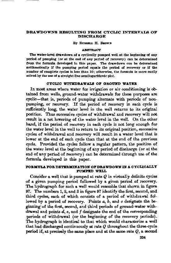
DRAWDOWNS RESTTI/TING FROM CTCLIC INTERVALS OFDISCHARGE

By RUSSELL H. BBOWN

ABSTRACT

The water-level drawdown of a cyclically pumped well at the beginning of any period of pumping (or at the end of any period of recovery) can be determined from the formula developed in this paper. The drawdown can be determined arithmetically if the pumping period equals the period of recovery or if the number of complete cycles is less than 10; otherwise, the formula is more easily solved by the use of a straight-line semilogarithmic plot.

CYCLIC WITHDRAWALS OF GROUND WATER

In most areas where water for irrigation or air conditioning is ob tained from wells, ground-water withdrawals for these purposes are cyclic that is, periods of pumping alternate with periods of non- pumping, or recovery. If the period of recovery in each cycle is sufficiently long, the water level in the well returns to its original position. Thus successive cycles of withdrawal and recovery will not result in a net lowering of the water level in the well. On the other hand, if the period of recovery in each cycle is not long enough for the water level in the well to return to its original position, successive cycles of withdrawal and recovery will result in a water level that is lower at the end of each cycle than that at the end of the previous cycle. Provided the cycles follow a regular pattern, the position of the water level at the beginning of any period of discharge (or at the end of any period of recovery) can be determined through use of the formula developed in this paper.

FORMULA FOR DETERMINATION OF DRAWDOWN IN A CYCLICALLYPUMPED WELL

Consider a well that is pumped at rate Q in virtually definite cycles of a given pumping period followed by a given period of recovery. The hydrograph for such a well would resemble that shown in figure 97. The numbers 1,2, and 3 in figure 97 identify the first, second, and third cycles, each of which consists of a period of withdrawal fol lowed by a period of recovery. Points a, &, and c designate the be ginning" of the first, second, and third periods of ground-water with drawal and points d, e, and / designate the end of the corresponding periods of withdrawal (or the beginning of the recovery periods). The hydrograph is identical to that which would characterize a well that had discharged continuously at rate Q throughout the three-cycle period if, at precisely the same place and at the same rate Q, a second

324


Effect of first discharging well

FIGURE 97. Hydrograph for a cyclically pumped well showing the symbolism used for time factors.

well had begun recharging at time d, a third well had begun discharg ing at time 6, a fourth well had begun recharging at time e, a fifth well had begun discharging at time <?, and a sixth well had begun recharg ing at time /. Thus the net drawdown in the real pumped well at the end of the third cycle can be expressed as follows:

S «r «r, (1)

where the numbered ^-subscripts refer to the discharging wells during the first, second, and third cycles, respectively, and the numbered r-subscripts refer to the respective recharging wells. Inasmuch as the net drawdown is to be computed for the pumped well (that is, the radius r in the basic Theis equation is small), the approximate form of the Theis (1935, p. 522) equation can be used for values of time that are not too small. Also, if the component drawdown s^ paired with the component buildup, or negative drawdown, sri> the expression for their algebraic sum is identical with the Theis recovery formula. Thus,

264Q, *!S^ «rj= y-lOg p>

_ =264g

. _264Q

tog 7^lz

(2)

(3)

(4)


Equation 1, which is the sum of equations 2, 3, and 4, can therefore be written as

"3 rrt "

The form of this equation suggests a simple expression for the draw down after any number of cycles. Thus, the drawdown in the pumped well immediately after completion of the nth cycle and immediately before the beginning of the (n-f 1) pumping period is

From figure 97, each cycle is seen to span a time interval of length t. Furthermore, within each cycle, the recovery interval spans a time interval of length tr and pumping occurs over a time span />£, where p represents the pumping fraction of the cycle (that is, the ratio of pumping time to the period of the cycle, t) . Therefore, each time factor appearing in equation 6 can be replaced by an equivalent factor written in terms of p and t.

The time factors for the discharging wells can be replaced by mul tiples of t; figure 97 shows that, for the nth cycle, tn can be replaced by t- for the last two cycles, £n_i can be replaced by 2£; for the last three cycles, tn-z can be replaced by 3£; and so on through the first cycle, for which £t can be replaced by nt.

In similar fashion, substitutions can be made for the time factors related to the recharging wells. Thus, for the nth cycle, tn' can be replaced by (t pt) £ _/, for the last two cycles, can be replaced by (2£ pt) tn-z ', for the last three cycles, can be replaced by (3£ pt) ; and so on through the first cycle for which £/ can be replaced by the factor (nt pt). Now equation 6 can be rewritten as follows:

Cancelling the t in each factor in the numerator with the t in the corresponding factor in the denominator and reversing the order of the two series gives the relation

-n "|

-p)]'-p) . . . (n

Therefore, the length of the cycle and the total length of time are seen to have no significance; the drawdown is determined by the number of cycles and not by whether those cycles are measured in minutes, days, years, or any other time unit.

PERMEABILITY, TRANSMISSIBILTTY, AND DRAWDOWN

Equation 8 can also be written in the form

327

(9)

A semilog plot of values of snT/Z§±Q on the arithmetic scale against values of n on the logarithmic scale for various values of p (see fig. 98) facilitates the solution of the equation. The change in the factor

2.8

2.4

2.0

1.6

1.2

0.8

0.4

0.010

p=0.25

20 40 60 80 100

FIGURE 98. Semilog plot of the factor *.T/264Q against the number of pumping cycles n for selectedvalues of p.


sn7'/264<2 during the nth cycle is represented by the last term of the series expression,

n-p

On the semilog plot, the increment on the n-axis during the nth cycle (that is, between points n 1 and n) is log n log(n 1), or

Therefore, the limiting slope of this semilog plot the slope across the nth cycle is given by the change in the factor sn7V2640 divided by the change in log n. In mathematical terms, this limiting slope for the nth cycle is

=r~2 (^=r) +3 (^=i) " J2 - 3

The series expansions for the two log terms can be found in most comprehensive handbooks of chemistry, mathematics, or physics. (See, for example, Hodgman, 1952, p. 274.) The expansions generally are given for the natural logarithm but are readily converted to the common logarithm by multiplying by 2.3.

If the two series expressions shown in equation 10 are multiplied by (n 1) , then the ratio becomes

P

n-l

As n approaches infinity, the value of this fraction approaches the quantity p. In other words, p is the limiting slope of the semilog plot previously described. Thus, a means for handily resolving equation 8 begins to emerge.


Note that equation 8 can be rewritten in the form

(11)The right half of this equation can be evaluated for the end of any number of cycles, w, and for the value p. For example, if p=Q.f5 and n=100, then

^gL=log 100!-(log 0.25+log 1.25+log2.25+. . .+log 99.25)=2.060.

Computations of this nature have been made for selected values of n and p. The results of these computations are given below and are plotted in figure 98.

Number of cycles (n)

10-.----20--_--_30------40----.-50.-.-..60.--__-70-----.80.-..--90-__-._100..--.

Valueof»n77264Q

p=0.25

0 342 416 459 490 514 534 550 565 577 589

p=0.50

0.754 .902 . 989

1.051 1. 100 1. 139 1. 172 1. 201 1. 226 1.249

p=0.75

1.313 1.537 1. 669 1.762 1.834 1.894 1.946 1.987 2.025 2.060

Observe that within the limits of plotting accuracy each curve shown is a straight line over the log cycle from n= 10 to n=lQQ. Further more, the slope of each of these curves is only a few tenths of one per cent less than the limiting slope p. General rules of procedure for the solution of practical field problems can now be stated.

When n is less than 10, solve equation 11 numerically, computing the factor s»77264$ in the manner indicated by the example. When n is more than 10 but less than 100, solve equation 11 graphically by use of figure 98. The family of curves shown in the figure can be ex panded easily to include any other value of p merely by computing the factor snT/264Q for w=10 and n=100, plotting the two computed values, and joining them by a straight line.

When n is greater than 100, find the value of s1007V264$ by com putation or from figure 98. The value for the end of the nth cycle can then be computed by using the relation

SnT

264Q"n (12)


Although it is an approximation, equation 12 gives values of that are only a few tenths of one percent too high. Because equation 12 is based on the idea of extending the lines in figure 98 beyond the 100th cycle, values of 8nT/^AQ for values of n greater than 100 can be determined without computation by extending the lines in figure 98 an appropriate distance beyond the n=100 ordinate.

When the pumping and recovery periods are of equal length that is, when p=0.5 equation 9 can be simplified for an easier solution as follows :

1.2-3.4-5- ...... -n "I-l*-2*-3H*. - . -<n-i) J

, - .4-6-8- g . 2n)

In any of the above methods, after the value of the log term is determined, the drawdown, sn. of the pumped well at the end of the nth cycle is readily found by multiplying the value of the log term by 264^/T7.

ESTIMATING THE TRANSMISSIBILITY OP AQUIFERS FROM THE SPECIFIC CAPACITY OF WELLS

By CHARLES V. THEIS, RUSSELL H. BROWN, and REX R. METER

ABSTRACT

The specific capacity of a well can be used as a basis for estimating the coefficient of transmissibility of the aquifer tapped by the well. From as sumed values for the hydrolojric constants of the aquifer, separate formulas including a term for specific capacity are develoi>ed for the transmissibility of water-table and artesian aquifers. Prom a chart relating the well diameter, the specific capacity of the well, and the coefficients of transmissibility and storage, the transmissibility of the aquifer can be estimated from the known specific capacity of the well or the specific capacity of the well can be estimated from the known transmissibility of the aquifer. These methods are subject to limitations but are useful means of approximation.

THE GENERAL RELATIONSHIP BETWEEN TRANSMISSIBILITY ANDSPECIFIC CAPACITY

In many ground-water investigations, especially those of a recon naissance type, the specific capacities of wells provide the only basis for estimating the transmissibility of the aquifers tapped by the wells. Generally speaking, high specific capacities indicate an aquifer having a high coefficient of transmissibility, T7, and low specific ca pacities indicate an aquifer having a low T. However, a precise cor relation between the specific capacities of wells and the T values of the aquifers they tap has not yet been established.

The specific capacity of a well cannot be an exact criterion of T in the vicinity of the well because, obviously, the yield of the well per foot of drawdown is also a function of other factors such as the diam eter of the well, the depth to which the well extends into the aquifer, the type and amount of perforation in the well casing, and the extent to which the well has been developed. However, estimates of T that are based on the specific capacities of wells should be reasonably re liable and could be made without the elaborate tests necessary for precise determinations. Therefore, if developed within the limits of idealized assumptions, a formula expressing the theoretically exact relationship between the specific capacity of a well and the trans missibility of the aquifer which the well taps would be highly useful n the making of reconnaissance ground-water studies provided the

Jieoretical formula is empirically modified for prevailing field conditions.

331


ESTIMATING THE TRANSMLSSIBILIT Y OF A WATER-TABLE AQUIFER FROM THE SPECIFIC CAPACITY OF A WELL

By CHARLES V. THEIS

The relation between the discharge of a well and the water-level drawdown a short distance from the well is given by an equation derived by Theis (1935). The value of u in that equation is small provided r is small, T and S are within the range of values for fairly productive aquifers, and t is at least several hours. For the purpose of this paper, the Theis formula can be written with negligible error as follows :

(i)

The computation can be made somewhat simpler by substituting values for S and T that are within the range of fairly productive water-table aquifers. However, if corrections for these values are included, the formula remains general. Thus, if T 1,000 gpd per ft, $=0.2, and t=l day, the formula for an average water-table aquifer corrected for variations of that aquifer from average is

(3 w 10-,) _logi

Therefore,

s s s

[-loglo (3.74f* 10- 6)-log10 5S+log10 t].

Let

then

< 10-6) _logio 5S+loglo t]s s

=2 [-66-264 log,0 (3.74r2 - 10~ 6)-264 Iog10 5S+264 Iog10 *]. s

Let

then


#=-66-264 Iog10 (3.74T-2 - 10' 6) (3)

(4)'= CK-264 log,0 5S+264 Iog100-s

Values of K, computed for selected values of r, are as follows:

r (ft)

0. 25. 501.05. 010

K

1,6841,5241,367

996838

r(ft)

20304050

K

680588521469

The foregoing formulas indicate the importance of both the stor age coefficient and the duration of pumping when the coefficient of transmissibility is estimated from a single measurement of drawdown in an observation well. If $=0.2, the influence of the S term is zero because the formula was derived on that basis. However, if $=0.1, the S term would equal 264 Iog10 5$= -264 Iog10 0.5=80, or about 8 percent of the constant, K, for r=5 .feet, and if $=0.3, the S term would equal 45, or about 4.5 percent of the same value for K. Provided S is known, the correction can be made, but if S is unknown, the error for a water-table aquifer (for which S ranges from 0.1 to 0.3) probably will be smaller than the errors inherent in the method. Although the correction for the duration of pumping also is com paratively small, it presumably should .be made if, as in many cases, the duration is known. For an artesian aquifer, S is very small and the S term correction will be large, making it inadvisable to apply the formula (in its present form) for artesian conditions; for if $=0.001, the S term would be about double K for r=5 feet.

The coefficient of transmissibility cannot be determined explicitly from the computed values of T'. However, from charts giving the values of Tf for various values of T and Q/s, the value of T can be ascertained from known values of T' and Q/s. Such a chart is shown in figure 99.

Thus, within the limits of the idealized assumptions, the coefficient of transmissibility of a water-table aquifer apparently can be com puted without great error from a single measurement of drawdown in an observation well that is a short distance from a pumped well, even if the coefficient of storage is not known. However, the informa-

690-185 o es 7


tion generally available concerns the specific capacity of the pumped well. In the foregoing formulas Q represents the discharge of the pumped well and * is the drawdown in a nearby observation well at a distance r from the pumped well. Obviously, the drawdown in the pumped well bears a relationship to the drawdown a short distance from the well. If this relationship can be ascertained approximately,

200

180

8

160

140

120

100

20

0 10 20 30 40 50 60 70

SPECIFIC CAPACITY, IN GALLONS PER MINUTE PER FOOT OF DRAWDOWN

FIGURE 99. Diagram for estimating the transmissibility of an aquifer from the specific capacity of a well.


the specific capacity of the pumped well can be substituted for the quantity Q/s for the appropriate distance from the well.

For small- diameter uncased wells that tap consolidated water bearing rocks, or at least for wells that produced no sand or silt when developed, the distance r probably can be equated to the radius of the well. For instance, for a well 6 inches in diameter,

7"=C(l,684-264 log 10 5£+264 Iog10 *), in which

C= = the specific capacity of the pumped well.o

In wells having perforated casing and for which no improvement in performance was noted upon development, some head is lost as the water moves through the perforations in the casing. The amount of head lost in this manner ranges widely according to whether or not the casing fits snugly against the wall of the hole. If it does, the drawdown within the aquifer at the wall of the hole presumably would be considerably less than within the well itself, and the specific capacity computed on the basis of the lesser drawdown would be con siderably higher. An arbitrary increase, then, in the specific capacity probably would be justified for the computation of the coefficient of transmissibility. In consolidated formations in which the wall of a hole is rough and the casing does not fit tightly, the loss in head pre sumably is small and can be disregarded.

Many wells of large yield tap aquifers that consist of consolidated sand or gravel. Such wells yield readily to development and once they are developed the pumping level of the water both within and immedi ately outside the casing is generally higher than it would have been had they not been developed. It is difficult to estimate the extent to which the transmissibility of the materials in the immediate vicinity of a well has been increased by the development of the well. How ever, available data indicate that in many cases the effect is the same as if the well were 10 feet in diameter but had not been developed. Therefore, 996 (the factor for r=5 ft) would be a reasonable value to substitute for K in the equation for T' '.

Although many empirical data should be gathered as to the relation between the specific capacities of wells and the transmissibilities of the tapped aquifers before any final correlation is made, present knowledge seems to justify the following equation for wells that have a diameter of about 1 foot and that tap water-table aquifers consisting of unconsolidated sediments:

,300-264 log

The factor (1±0.3) should be adjusted upward for wells having a

336 GROUND'WATER HYDRAULICS

small diameter, for wells that are poorly developed, and for wells with poorly perforated casing, and downward for larger and well-developed wells.

ESTIMATING THE TRAN8MIS8IBILITY OF AN ARTESIAN AQUIFER FROM THE SPECIFIC CAPACITY OF A WELL

By RUSSELL H. BROWN

The use of figure 99 can be demonstrated by the following example. Assume that examination of well logs and related data has led to an estimate of 0.15 as a likely coefficient of storage, $, for a given water- table aquifer, that a review of well records has revealed a number of completion (or acceptance) tests, and that data taken from the best controlled test show, for a 30-hour pumping period, the specific capac ity of a 6-inch well to be 12 gpm per ft of drawdown. The order of magnitude of the coefficient of transmissibility is to be determined. From the preceding discussion by Theis,

r= (#-264 log105S+264 loglo*)o

= 12(1,684-264 log100.75-|-264 Iog101.25)= 12(1,684-1-33-1-26)=20,900.

As shown by figure 99, the abscissa of Tf 20,900 gdp per ft intersects the ordinate of specific capacity equals 12 gpd per ft of drawdown about where 7*= 19,000 gpd per ft. If S should later prove to be 0.25 instead of 0.15, the revised value of Tf would be 20,200 and, from the chart, T would be about 18,000 gpd per ft. Thus it is evident that even large differences in S do not materially affect the value of T and that exercising judgment in selecting a value for S will produce results of the correct order of magnitude.

As stated by Theis (p. 333), the formulas and related constants de rived by him are not applicable to artesian conditions. The principal objection in attempting to extend their application from water-table conditions to artesian conditions is the large adjustment in the K factor that becomes necessary if, for example, £=2X10-*, which is one-thousandth the assumed £=0.2. However, a formula and set of constants for artesian conditions can be found by paralleling the Theis derivation and using an assumed coefficient of storage of 2 X 10~4 . If it is assumed again that T= 100,000 gpd per ft, Theis' diagram (fig. 99) can be used without modification.


If T= 100,000 gpd per ft and S=2X 10~4, then from equation 1 on page 332

114.6g r /1.87r» . 2 1Q-* S 100,000 IV]1 r~ L~°-577~log<V Topoo 2 . io-*r ' t)\(3.74r».10-«)(5S.l(

-Iog10 (58 10«)+logio (T 10-6)+log10*].

Therefore,

Again let

Then

s s

-Iog10 (3.74r* - 10-»)-log10 (58 103)+log10 *].

10_6)

=[-66-264 log,0 (3.74T-2 10-»)-264 log,0 (58

Let

= -66-264 log,o (3.73r2 lO"9).

Then

T'=Q [#-264 log,0 (58 10")+ 264log,0*]. s

Values of K, computed for selected values of r, are as follows:

logic*]

(5)

(6)

r(ft)

0.25.501.05.010

K

2,4772,3182,1591,7901,633

r(ft)

20304050

K

1,4721,3791,3131,262


If the value of S is as large as 2X10"3 (10 times the,assumed value) the effect will be to decrease K for r 5 feet by nearly 15 percent. For larger values of K this percentage obviously is lower, and for smaller values it is higher. Conversely, if 8 is as low as 2X 10~5 (one tenth the assumed value) the effect will be to increase K by nearly 15 percent.

The application of the equation derived for T' for artesian condi tions can be demonstrated by an example. Assume that the best esti mate of S for a given artesian aquifer is 4X10~5 . Furthermore, data collected during a 30-hour acceptance test of a 6-inch well show that the specific capacity of the well is 7.5 gpm per ft of drawdown. The coefficient of transmissibility may be computed by following the same procedure used in the previous example. Thus,

7" =2 [#-264 log,0 (5S 103) +264 Iog10«] s=7.5(2,477-264 log,0 0.2+264 log,0 1.25)=7.5(2,477+184+26)=20,200.

According to figure 99, T= 18,000 gpd per ft (approx.) where the ordinate of 7.5 intersects the abcissa of 20,200. If it later develops that a value of 4X 10~4 is a better estimate of £, then T' would be 18,200 and T would be about 16,000 gpd per ft.

A CHART RELATING WELL DIAMETER, SPECIFIC CAPACITY, AND THE COEFFICIENTS OF TRANSMISSIBILITY AND STORAGE

By REX R. METEB

The relationships of well diameter, specific capacity, and the coeffi cients of transmissibility, T7, and storage, S, are shown graphically in figure 100. This graph was prepared by (1) computing, for various values of T and S, the theoretical drawdown in wells having diameters of 6, 12, and 24 inches, (2) computing the specific capacity of those wells (on the assumption that they are 100 percent efficient), and (3) plotting the specific capacity against S to form a family of curves which represent the different values of T. For the sake of clarity, the curves for a well 24 inches in diameter were not plotted in the upper part of the graph; they would be virtually parallel to the curves for a well 12 inches in diameter and lie above them at a distance equal to that between the curves for wells 6 inches and 12 inches in diameter. The specific capacity at the end of 1 day's pumping is shown on the left scale of the graph. The values of S, shown on the bottom scale, range from those for artesian conditions on the left to those for water- table conditions on the right. Each group of curves for a specific T is bracketed on the right margin.


Figure 100 can be used to determine the approximate T of an aquifer if the specific capacities of wells are the only available data. It also can be used to determine the approximate specific capacity of a well which is to be drilled into an aquifer for -which T and S are known. The computed theoretical specific capacity is useful not only for plan ning purposes but also, when compared to the specific capacity deter mined from a field test, as a means of determining the approximate efficiency of a well. Although determinations made from figure 100 may not be exact owing to unknown factors that must be estimated, the graph serves as a measure for approximation.

A cursory study of the graph reveals that it has certain limitations. One of the principal factors affecting the specific capacity of a well is the entrance loss of the water. The graph is based on the assump tion that the wells are 100 percent efficient or, in other words, that when the wells are pumped the water level inside and immediately outside the casing or screen is the same. Because, in most wells, the water level immediately outside is higher than inside, the observed specific capacity is somewhat less than that of an ideal well. The specific capacity of a well is affected also by the diameter of the well. The well diameters shown on the graph 6, 12, and 24 inches are considered to be the effective diameters of the wells. If an aquifer is composed of consolidated rocks, the effective diameter probably is approximately the same as the diameter of the well. However, if the material in an aquifer consists of unconsolidated materials and if

200

} 200,000 " }150,000£100,000^;80,000 < 60,000 °

}40,000 £

Well is assumed to have 100 percent efficiency, , , i ,.,,1 , ,

0.00001 0.00005 0.0001 0.0005 0.001 0.005 0.01 0.05 0.1 COEFFICIENT OF STORAGE

FIQUBE 100. Graph showing relation of well diameter, specific capacity, and coeflBclents of transmlsslbllltyand storage.


the well has been highly developed, the effective diameter may be sub stantially larger than the diameter of the screen. On the other hand, a seemingly highly developed well may be very inefficient because of caving or faulty construction, and, accordingly, have an effective di ameter less than the diameter of the screen. Other conditions being the same, a change in the effective diameter has the greatest effect on the specific capacity of wells in aquifers that have a low T and a high S.

The graph shows that large changes in /S correspond to relatively small changes in T and specific capacity; therefore, inaccuracy in estimating S generally is not a serious limiting factor. Moreover, from a general knowledge of the geology and hydrology, an aquifer usually can be classified as principally water table or artesian, and S can be estimated accordingly. However, the graph should not be used in an attempt to determine 8 even when accurate values of the specific capacity and T are available.

If the pumped well taps less than the full thickness of the aquifer thus introducing vertical components of flow or if it taps a thin water-table aquifer so that the water-level drawdown is a substantial fraction of the original saturated thickness, the graph obviously can not be applied without serious error.

The time interval of 1 day used for computing the specific capacity scale on the graph was selected arbitrarily. An error will be intro duced if the specific capacity determined in the field is based on a shorter or longer period of pumping. The amount of the error is small for high values of T and low values of /S but increases substan tially for low values of T and high values of S.

The procedure for using the log graph to determine T from the specific capacity of a well is as follows:

1. Select the specific capacity on the left margin.2. Move horizontally along the abcissa to the intersection of the ordinate

through the estimated value of S.3. From this intersection move along a curve or parallel to the family of

curves, and find the value of T on the right margin.

Although the specific capacity at the end of 1 day's pumping can be computed for an ideal well tapping an aquifer having known values of T and $, it can be determined more easily and quickly from the graph. To determine the theoretical specific capacity of such a well, the procedure described above is reversed; move left along or parallel to the curve from the known value of T to the intersection of the ordinate through the known value of S ; thence move horizon tally to the left margin and read the specific capacity.

If the graph is used with an understanding of its limitations, it should provide a useful tool in ground-water studies.


REFERENCES CITED

Barksdale, H. C., Sundstrom, R. W., and Brunstein, M. S., 1936, Supplementaryreport on the ground-water supplies of the Atlantic City region : New JerseyState Water Policy Comaa., Spec. Kept. 6.139 p.

Carslaw, H. S., 1945, Introduction to the mathematical theory of the conductionof heatTn solids: New York, Dover Publications, 268 p.

Carslaw, H. S., and Jaeger, J. C., 1947, Conduction of heat in solids: London,Oxford Univ. Press, 386 p.

Dupuit, Jules, 1863, Etudes theoriques et pratiques sur le mouvement des eauxdans les canaux decouverts et a travers les terrains permeables: 2d ed,Paris, Dunod, 304 p.

Ferris, J. G., 1950, A quantitative method for determining ground-water char acteristics for drainage design: Agr. Eng., v. 31, no. 6, p. 285-291.

Hodgman, C. D., 1952, Handbook of chemistry and physics: 34th ed., Cleveland,Ohio, Chemical Rubber Pub. Co., 2950 p.

Ingersoll, L. R., Zobel, O. J., and Ingersoll, A. C., 1948, Heat conduction; withengineering and geological applications: New York, McGraw-Hill Book Co.,278 p.

Jacob, C. E., 1940, On the flow of water in an elastic artesian aquifer: Am.Geophys. Union Trans., pt. 2, p. 585-586.

1950, Flow of ground water, in Rouse, Hunter, (ed.), Engineering hydraulics, chap. 5: New York, John Wiley & Sons, p. 321-386.

Kozeny, J., 1933, Theorie und Berechnung der Brunnen: Wasserkraft und Wasserwirtschaft, v. 28, p. 88-92, 101-105,113-116.

Muskat, Morris, 1932, Potential distributions in large cylindical discs [homoge neous sands] with partially penetrating electrodes [partially penetrating wells] : Physics, v. 2, no. 5, p. 329-384.

1937, The flow of homogeneous fluids through porous media: New York, McGraw-Hill Book Co., 763 p.

Peirce, B. O., 1929, A short table of integrals: Boston, Ginn & Co., 156 p.Rambaut, A. A., 1901, Underground temperature at Oxford in the year 1899, as

determined by five platium-resistance thermometers: Royal Soc. [London] Philos. Trans., ser. A., v. 195, p. 235-258.

Theis, C. V., 1935, The relation between the lowering of the piezometric surface and the rate and duration of discharge of a well using ground-water storage: Am. Geophys. Union Trans., 16th Ann. Mtg., pt. 2, p. 519-524.

Thompson, D. G., 1928, Ground-water supplies of the Atlantic City region: New Jersey Dept. Conserv. and Devel. Bull. 30, 138 p.

Wenzel, L. K., 1936, The Thiem method for determining permeability of water bearing materials and its application to the determination of specific yield, results of investigations in the Platte River Valley, Nebr.: U.S. Geol. Survey Water-Supply Paper 679-A, 57 p.

1942, Methods for determining permeability of water-bearing materials, with special reference to discharging-well methods, with a section on Direct laboratory methods and a Bibliography on permeability and laminar flow by V. C. Fishel: U.S. Geol. Survey Water-Supply Paper 887, 192 p.

Werner, P. W., and Noren, Daniel, 1951, Progressive waves in non-artesian ground-water aquifers: Am. Geophys. Union Trans., v. 32, no. 2, p. 238-244.

O

methods of determining - usgs · r. h. brown, j. g. ferris, ... the recovery method for determining...

Documents