methods to assess the impacts of subnational sustainability

Methods to assess the impacts of subnational sustainability

Takako Wakiyama

A thesis submitted in fulfilment of requirements for

the degree of Doctor of Philosophy.

Faculty of Science

School of Physics

University of Sydney

December 2019

2

Acknowledgement

I would like to thank my supervisor, Pref. Manfred Lenzen, for his kind support and guidance. Manfred

is the most academically and personally respected person I have ever had the good fortune to meet. I

would also like to give special thanks to Arne Geschke, Keisuke Nansai, Joy Murry and Tommy

Wiedmann, who have been exceptional mentors and supporters of my study and my career in research.

Thank you to my colleagues at ISA and to the friends I have met during my PhD work in Australia. I

have truly appreciated the opportunity to meet and become friends with all of them.

I also want to thank my colleagues at the Institute for Global Environmental Strategies (IGES) for their

outstanding support. My study has been financially supported by the Environment Research and

Technology Development Fund (1-1703) of the Environmental Restoration and Conservation Agency

of Japan, by the National eResearch Collaboration Tools and Resources project (NeCTAR) through its

Industrial Ecology Virtual Laboratory VL201, and by the Australian Research Council (ARC) through

its Discovery Projects DP0985522 and DP130101293, and through IELab infrastructure funding

LE160100066. Without the support of IGES, Manfred Lenzen, Arne Geschke, Joy Murry and Tommy

Wiedmann, I would not have been able to pursue my PhD.

Last but not least, I want to thank my parents, grandparents, aunts and uncles, who have always

supported and encouraged me whenever I set out on a new journey. Special appreciation to my mother,

Hisako Wakiyama, and grandmothers, Ryoko Wakiyama and Miyo Sekine, whom I deeply respect for

the lives they have lived, always with a positive mind, dedication, patience, respect and thoughtfulness

towards others during particularly difficult times for women. They have encouraged me to be a positive

and independent woman, and to find happiness and freedom on my own terms and under any

circumstances.

3

Originality

This is to certify that to the best of my knowledge, the content of this thesis is my own work. This thesis

has not been submitted for any degree or other purposes.

I certify that the intellectual content of this thesis is the product of my own work and that all the

assistance received in preparing this thesis and sources have been acknowledged.

Takako Wakiyama

4

Abstract

Environmental, social, and economic problems, such as global warming, natural disasters, urbanization,

and poverty, are interlinked and become more complexly entwined under globalization. In 2015,

recognizing global problems such as these, all United Nations member states adopted the 2030 Agenda

for Sustainable Development, which outlines sustainable development goals (SDGs). At the same time,

the United Nations Framework Convention on Climate Change (UNFCCC) adopted the Paris

Agreement, which has the long-term goal of mitigating greenhouse gas (GHG) emissions; each nation

is expected to increase its mitigation target in order to limit global warming to less than 2 degrees

Celsius. To achieve the goals set out in the international agreements, nations need to identify problems

and assess the impact of these problems at the subnational level, not only on a national and worldwide

scale. In fact, there is an ever-growing need to construct a subnational analysis tool to identify problems

and find solutions using micro- and macro-analytical tools, such as a multiregional input–output

(MRIO) database.

The main aim of this thesis is to develop models for sustainability analysis at the subnational level and

apply them to assessing environmental, economic, and social impacts. To this end, a cloud-computing

platform called the Japan Industrial Ecology Laboratory (IELab) was developed. The IELab is highly

flexible in terms of its sectoral and regional resolution—enabling users to build customized Japanese

MRIO tables in accordance with their specific objectives. A subnational MRIO analysis can track inter-

regional trade for cities, counties, or states within a country. Footprint analysis conducted using the

MRIO database can help fill in information gaps between producers and consumers on various

economic, social, and environmental issues. In the case study, food loss analysis was conducted to

examine regional food loss, not only from a production perspective, but also from a demand-side. As

another subnational analytical method, a bottom-up technology model was presented as CO2 emission

mitigation as an example. Using the model, the impact of future technological changes in the regional

electricity system on Japan’s overall energy mix was assessed.

5

Attribution

Chapter 2 of this thesis is published as:

- Wakiyama, T., Lenzen, M., Geschke, A., Bamba, R., Nansai, K. (2020). A flexible

multiregional input–output database for city-level sustainability footprint analysis in Japan.

Resources, Conservation and Recycling, 154.

I designed the study, performed data extraction and analysis, wrote the manuscript and acted as

corresponding author.


- Wakiyama, T., Lenzen, M., Faturay, F., Geschke, A., Malik, A., Fry, J., Nansai, K. (2019).

Responsibility for food loss from a regional supply-chain perspective. Resources, Conservation

and Recycling, 146, 373-383.




- Fry, J., Lenzen, M., Jin, Y., Wakiyama, T., Baynes, T., Wiedmann, T., Malik, A., Chen, G.,

Wang, Y., Geschke, A. (2018). Assessing carbon footprints of cities under limited information.

Journal of Cleaner Production, 176, 1254-1270.

I assisted in designing the study and performed data extraction and analysis.


- Wakiyama, T., Kuriyama, A. (2018). Assessment of renewable energy expansion potential and

its implications on reforming Japan's electricity system. Energy Policy, 115, 302-316.



6

Other publications resulting from this PhD, but not included in this thesis:

- Ninpanit, P., Malik, A., Wakiyama, T., Geschke, A., Lenzen, M. (2019). Thailand's energy-

related carbon dioxide emissions from production-based and consumption-based perspectives.

Energy Policy, 133, 1-11.

- Wakiyama, T. Ghana’s agricultural and water footprint analysis. Book Chapter. Submitted to

Book “A Triple Bottom Line Analysis of Global Consumption”. Submitted to editors

In addition to the statements above, in cases where I am not the corresponding author of a published

item, permission to include the published material has been granted by the corresponding author.

Takako Wakiyama

As supervisor for the candidature upon which this thesis is based, I can confirm that the authorship

attribution statements above are correct.

Manfred Lenzen

7

Acronyms

ALIC Agriculture & Livestock Industries Corporation

AMeDAS Automated Meteorological Data Acquisition System

CO2 Carbon dioxide

ECBA Economic Census for Business Activity

EROT Electric Reliability Council of Texas

FERC Federal Energy Regulatory Commission

FIT Feed-in tariff

FLQ Flegg's location quotient

GHGs Greenhouse gas

GPC Community-Scale Greenhouse Gas Emission Inventories

GUI Graphical user interface

GWh Gigawatt-hours

IEA International Energy Agency

IELab Industrial Ecology Laboratory

IO Input-output

IOA Input-output analysis

IPPs Independent power producers

ISOs Independent system operators

KRAS Scaling optimization method

LCA Life-cycle assessment

MAFF Ministry of Agriculture, Forestry and Fisheries

METI Ministry of Economy, Trade and Industry

MLIT Ministry of Land, Infrastructure, Transport and Tourism

MOE Ministry of the Environment

MRIO Multiregional input-output

MWh Megawatt-hours

8

NDCs Nationally determined contributions

NRA Nuclear Regulation Authority

PIRR Project internal rate of return

RemC Remainder of country

RoW Rest-of-World

RPS Renewable portfolio standards

PV Photovoltaics

RTOs Regional transmission organizations

SCP Sustainable consumption and production

SDGs Sustainable Development Goals

SPP Southwest Power Pool

TWh Terawatt-hours

3EID Embodied Energy and Emission Intensity Data

9

Life is like mountaineering. Mountaineering naturally opens our eyes, through the encounters we have

with other people on the way to a summit. On our way to the summit, we experience hard times and

beautiful moments. There are many ups and downs. Nature makes us appreciate that we live on an

amazing planet, but at the same time, it makes us realize that there are things we do not expect and

situations we cannot control—and nor do we wish that we could. We also realize that we always have

someone around to encourage us, support us, and care about us: someone to climb with to the summit,

to share both fun and hard times, and to show us our directions.

I appreciate everyone I have met in my life. I would not be here without the people with whom I have

shared experiences, who have inspired and supported me. In my journey and adventure on my way to

the summit, I discover new worlds and realize the kindness of the people around me. As in research,

there are many things in life that we have not yet discovered. We will always be able to find something

that we have not done before, if we sustain interest, curiosity, and a desire to explore, and if we do not

give up.

Adventure is a road we choose to take. There are many options for our lives. With a bit of courage to

jump into new worlds, we might take a backpack and go anywhere our inspirations direct us, or

anywhere we choose. Then, we might find something we have never before discovered or imagined.

There are no meaningless things or times in our lives if we use them to take one step toward a goal. If

we encounter a problem that is hard to solve, we must be patient for a while and wait until the moment

is blown away, or the sun comes out on us. The hard times will be just tiny moments in the long-time

journey of our lives.

10

Contents 1. Introduction ................................................................................................................................ 12 2. A flexible multiregional input–output database for city-level sustainability footprint analysis in Japan ............................................................................................................................................... 19

2.1. Introduction .................................................................................................................. 19 2.2. Methodology ................................................................................................................. 21

2.2.1. Overview of MRIO table-building with the Japan IElab ......................................... 21 2.2.2. Root table and initial estimate .................................................................................. 22 2.2.3. Creating the root table .............................................................................................. 22 2.2.4. Initial estimate of MRIO with the non-survey method ............................................ 25

2.3. Data feed constraints and reconciliation with optimization ........................................ 26 2.3.1. Data feed constraints ................................................................................................ 26 2.3.2. Reconciliation with optimization ............................................................................. 27

2.4. Results ........................................................................................................................... 28 2.4.1. Features of the Japan IELab ..................................................................................... 28 2.4.2. Case study 1: Building a prefecture-level MRIO ..................................................... 28 2.4.3. Diagnostic test in case study 1 ................................................................................. 30 2.4.4. Case study 2: Building a city-level MRIO ............................................................... 33 2.4.5. Diagnostic test in case study 2 ................................................................................. 35

2.5. Discussion ..................................................................................................................... 36 2.6. References ..................................................................................................................... 39 2.7. Supplementary information .......................................................................................... 46

3. Responsibility for Food Loss from a Regional Supply-Chain Perspective ............................... 53 3.1. Introduction ........................................................................................................................ 53 3.2. Methods and data ......................................................................................................... 57

3.2.1. Estimating regional food loss ................................................................................... 57 3.2.2. Subnational-level MRIO addressing the food supply system .................................. 58 3.2.3. Subnational-level MRIO calculations ...................................................................... 60 3.2.4. Environmental satellite data ..................................................................................... 62

3.3. Results ........................................................................................................................... 63 3.3.1. Regional characteristics of food loss ........................................................................ 63 3.3.2. Structure of food loss footprint by region ................................................................ 65 3.3.3. Environmental burdens related to the food loss footprint ........................................ 69

3.4. Discussion ..................................................................................................................... 70 3.5. References ..................................................................................................................... 73 3.6. Appendix ....................................................................................................................... 81

4. Assessing carbon footprints of cities ......................................................................................... 83 4.1. Introduction .................................................................................................................. 83

4.1.1. Input-output approach to footprint ........................................................................... 84 4.1.2. Aim of this study ...................................................................................................... 86

11

4.2. Methods and data ......................................................................................................... 87 4.2.1. Truncation errors associated with non-IO methods ................................................. 87 4.2.2. Effect of data quality on footprint measures ............................................................ 88 4.2.3. Comparisons between footprint results .................................................................... 93

4.3. Results ........................................................................................................................... 93 4.3.1. Carbon footprints of Beijing, Shanghai, Chongqing and Tianjin ............................ 93 4.3.2. Truncation errors ...................................................................................................... 99 4.3.3. Effect of deficiencies in the city IO database ......................................................... 100

4.4. Conclusions ................................................................................................................ 104 4.5. References ................................................................................................................... 106 4.6. Appendix ..................................................................................................................... 113

5. Assessment of renewable energy expansion potential and its implications on reforming Japan’s electricity system .......................................................................................................................... 125

5.1. Introduction ................................................................................................................ 125 5.2. Background and Literature Review ............................................................................ 126

5.2.1. Renewable potentials in Japan ............................................................................... 126 5.2.2. Conventional regional electricity system and challenges for renewable energy expansion 129 5.2.3. Scope of this paper ................................................................................................. 134

5.3. Methodology ............................................................................................................... 135 5.3.1. Input data ................................................................................................................ 136

5.4. Results ......................................................................................................................... 141 5.5. Discussion ................................................................................................................... 147 5.6. Limitations of this study .............................................................................................. 148 5.7. Conclusions and Policy Implications ......................................................................... 149 5.8. References ................................................................................................................... 151 5.9. Appendix ..................................................................................................................... 156

6. Conclusion ............................................................................................................................... 159

12

Chapter 1 Introduction

Globalization has revealed various economic, social, and environmental issues, such as economic and

social inequity, and environmental degradation throughout the world (Dabla-Norris, Kochhar,

Suphaphiphat, Ricka, & Tsounta, 2015; Lofdahl, 2002; Najam, Runnalls, & Halle, 2016). While natural

resources are exploited (using labor, land, water, and energy) in one region, they are manufactured and

consumed in other regions. Globalization expands the scope of human and economic interactions. The

trade of commodities has become intertwined with these interactions, making supply chains and their

associated risks harder to track (Heckmann, Comes, & Nickel, 2015). Every economic activity from

production to consumption requires inputs including resources and materials. Emerging problems such

as global warming and human trafficking highlight the importance of transparency in supply chains.

This is becoming an important political and economic issue, which governments and businesses need

to address and take action on at the local level (Birkey, Guidry, Islam, & Patten, 2018; Lenschow,

Newig, & Challies, 2016).

A substantial number of researchers have studied the supply chains of products using life cycle

assessment (LCA), hybrid LCA, and multiregional input-output (MRIO) analysis (Greschner

Farkavcova, Rieckhof, & Guenther, 2018; Moran, McBain, Kanemoto, Lenzen, & Geschke, 2015;

Pomponi & Lenzen, 2018; Zhao, Onat, Kucukvar, & Tatari, 2016). These studies use national data to

construct an overview of problems associated with the supply chains and to examine a trend of

commodity flow between nations. However, the exploitation of resources, labor, and the environment,

as well as the consumption of this exploitation, occur at the subnational level. To secure sufficient

transparency, it is crucial to identify supply chains from downstream, where natural resources are

exploited, to upstream, where the resources are consumed and used to produce products at the

subnational level—not only at the national level (Croft, West, & Green, 2018; WRI, C40, & ICLEI,

13

2014). There is an ever-growing need to construct a subnational analysis to identify problems and find

solutions using micro- and macro-analytical tools, such as a multiregional input-output (MRIO) analysis

(Faturay, Lenzen, & Nugraha, 2017; Lin, Hu, Zhao, Shi, & Kang, 2017; Mi et al., 2016; Wang, Geschke,

& Lenzen, 2017; Wiedmann et al., 2010). By identifying social, economic and environmental problems

in smaller administrative regions within a country from both production and consumption perspectives,

local government and businesses could implement practical plans and actions to mitigate those

problems. While environmental problems such as CO2 emissions can be mitigated by improving the

supply chain, emissions from direct economic operations should be reduced by improving the

operations and management of businesses. For instance, the CO2 emissions generated in a process of

production can be tracked by examining the supply chains. Consumers could indirectly reduce the CO2

emissions by changing the supply chains. On the other hand, CO2 emissions should be directly reduced

by changing the energy mix from energy-intensive sources, such as fossil fuels, to less energy-intensive

resources including renewables. To achieve this, potential areas for reducing CO2 emissions should be

also identified at the subnational level.

This thesis aims to develop two tools for sustainability analysis at the subnational level and apply them

to assess the environmental, economic and social impacts. "Sustainability" can be defined in many ways,

such as 'the long-term stability of the economy and environment' (Emas 2015, page 2) or conserving

resources for future generations (Bahadure, 2017; Shah, 2008). In terms of conserving resources for

future generations, we might consider preventing global environmental problems, such as global

warming, biodiversity loss, deforestation, desertification and water scarcity. In contrast, sustainability

can be defined more broadly as "intergenerational equity" (Dernbach 1998; Golub, Mahoney and

Harlow 2013), with an emphasis on maintaining the accessibility of food, water and resources for future

generations. In this thesis, sustainability is defined as securing access to resources for future generations

and preventing the negative environmental and social impacts of human activities on physical,

biological and human systems. For example, this thesis engages in an analysis of food security and

climate change.

14

Another important component of sustainability to consider is how to ensure sustainability in society.

Many scholars and practitioners, including international organizations such as the United Nations (UN),

have discussed sustainability as a global issue (Allen, Metternicht and Wiedmann 2016; UN 2015).

However, key actors to prevent environmental degradation and global warming are individuals and

governments at the local level because human activities are the main causes of these global problems

(Hale & Mauzerall, 2004; Salvia, Leal Filho, Brandli, & Griebeler, 2019). Actions are taken at the local

level, such as district and city, to build a sustainable future for cities. Actions for future sustainability

can be implemented by the government and citizens at the city level and also at the project level with

the collaboration of the community, government and private sectors. For example, a small-scale project

is required to improve natural habitats and reduce GHG emissions by transitioning from conventional

to environmentally friendly systems, such as renewable electricity generation.

Given the importance of actions and implementations at the subnational level, this thesis develops and

introduces tools to trace the link between local actors (producers) and local consumers and to assess the

impacts of both harmful and beneficial human actions, including economic activities and sustainable

system changes.

This thesis has the following research purposes:

Research purpose 1: To develop a city-level Japanese MRIO database that enables researchers,

policymakers, and businesses to create a customized MRIO table to assess the economic, social, and

environmental impacts of specific sectors and regions (Chapter 2).

Research purpose 2: To quantify regional food loss footprints in a case study of a subnational MRIO

database that is developed in Research purpose 1. To track where food loss occurs and where the

agricultural products, currently being discarded in fields, would presumably be delivered and consumed

(Chapter 3).

15

Research purpose 3: To examine potential errors and uncertainties associated with calculating cities’

carbon footprints, in order to identify levels of data availability that do not allow for the sufficiently

accurate calculation of carbon footprints (Chapter 4).

Research purpose 4: To employ a bottom-up technology model to assess how regional renewable energy

potentials can be put to effective use. It aims to introduce one example of various methods other than a

top-down approach introduced in Research purpose 1 to 3 in order to assess the impacts of subnational

sustainability. (Chapter 5).

As for the structure of this thesis, the first three chapters discuss the subnational footprint analysis as a

method of tracking the supply chains of products, for sustainable analysis. The following chapter focus

on identifying potential areas where CO2 emissions can be reduced at the subnational level, by using an

analytical tool to examine key factors in the energy system to mitigate CO2 emissions. Brief descriptions

of each chapter follow.

Chapter 2 describes a cloud-computing, city-level MRIO database for Japan, called the Japan Industrial

Ecology Laboratory (IELab). It is highly flexible in terms of its sectoral and regional resolution,

enabling users to build customized Japanese MRIO tables in accordance with their specific objectives.

Chapter 3 introduces a case study using the Japan IELab, focusing on Japan’s food loss at the

subnational level. Chapter 4 identifies the errors and uncertainties of city-level footprint analysis. It

shows conclusively that city carbon-footprint analyses should include input-output databases (and

associated calculus) to avoid severe errors. These errors arise from unacceptable scope limitations,

caused by the truncation of the footprint assessment boundary. Chapter 5 introduces another subnational

analytic tool, a bottom-up technology model. It assesses the impacts of future technological changes on

Japan’s overall energy mix. Chapter 6 presents conclusions and directions for further research.

16

References

Allen, C., Metternicht, G., & Wiedmann, T. (2016). National pathways to the Sustainable

Development Goals (SDGs): A comparative review of scenario modelling tools. Environmental

Science & Policy, 66, 199–207. https://doi.org/10.1016/j.envsci.2016.09.008

Bahadure, S. (2017). Power of Doubling: Population Growth and Resource Consumption.

International Journal of Urban and Civil Engineering, 11(7), 928–935.

Birkey, R. N., Guidry, R. P., Islam, M. A., & Patten, D. M. (2018). Mandated Social Disclosure: An

Analysis of the Response to the California Transparency in Supply Chains Act of 2010. Journal

of Business Ethics, 152(3), 827–841. https://doi.org/10.1007/s10551-016-3364-7

Croft, S. A., West, C. D., & Green, J. M. H. (2018). Capturing the heterogeneity of sub-national

production in global trade flows. Journal of Cleaner Production, 203, 1106–1118.

https://doi.org/https://doi.org/10.1016/j.jclepro.2018.08.267

Dabla-Norris, E., Kochhar, K., Suphaphiphat, N., Ricka, F., & Tsounta, E. (2015). Causes and

Consequences of Income Inequality: A Global Perspective. INEQUALITY: CAUSES AND

CONSEQUENCES INTERNATIONAL MONETARY FUND. Retrieved from

https://www.imf.org/external/pubs/ft/sdn/2015/sdn1513.pdf

Dernbach, J. C. (1998). Sustainable Development as a Framework for National Governance . Case

Western Reserve Law Review, 49(1). Retrieved from

https://scholarlycommons.law.case.edu/caselrevhttps://scholarlycommons.law.case.edu/caselrev/

vol49/iss1/3

Emas, R. (2015). The Concept of Sustainable Development: Definition and Defining Principles.

Faturay, F., Lenzen, M., & Nugraha, K. (2017). A new sub-national multi-region input–output

database for Indonesia. ECONOMIC SYSTEMS RESEARCH, 29(2), 234–251.

https://doi.org/10.1080/09535314.2017.1304361

Golub, A., Mahoney, M., & Harlow, J. (2013). Sustainability and intergenerational equity: do past

injustices matter? Sustainability Science, 8(2), 269–277. https://doi.org/10.1007/s11625-013-

0201-0

Greschner Farkavcova, V., Rieckhof, R., & Guenther, E. (2018). Expanding knowledge on

17

environmental impacts of transport processes for more sustainable supply chain decisions: A

case study using life cycle assessment. Transportation Research Part D: Transport and

Environment, 61, 68–83. https://doi.org/https://doi.org/10.1016/j.trd.2017.04.025

Hale, T. N., & Mauzerall, D. L. (2004). Thinking Globally and Acting Locally: Can the Johannesburg

Partnerships Coordinate Action on Sustainable Development? The Journal of Environment &

Development, 13(3), 220–239. https://doi.org/10.1177/1070496504268699

Heckmann, I., Comes, T., & Nickel, S. (2015). A critical review on supply chain risk – Definition,

measure and modeling. Omega, 52, 119–132.

https://doi.org/https://doi.org/10.1016/j.omega.2014.10.004

Lenschow, A., Newig, J., & Challies, E. (2016). Globalization’s limits to the environmental state?

Integrating telecoupling into global environmental governance. Environmental Politics, 25(1),

136–159. https://doi.org/10.1080/09644016.2015.1074384

Lin, J., Hu, Y., Zhao, X., Shi, L., & Kang, J. (2017). Developing a city-centric global multiregional

input-output model (CCG-MRIO) to evaluate urban carbon footprints. Energy Policy, 108, 460–

466. https://doi.org/https://doi.org/10.1016/j.enpol.2017.06.008

Lofdahl, C. (2002). Environmental Impacts of Globalization and Trade: A Systems Study.

Mi, Z., Zhang, Y., Guan, D., Shan, Y., Liu, Z., Cong, R., … Wei, Y.-M. (2016). Consumption-based

emission accounting for Chinese cities. Applied Energy, 184, 1073–1081.

https://doi.org/https://doi.org/10.1016/j.apenergy.2016.06.094

Moran, D., McBain, D., Kanemoto, K., Lenzen, M., & Geschke, A. (2015). Global Supply Chains of

Coltan. Journal of Industrial Ecology, 19(3), 357–365. https://doi.org/10.1111/jiec.12206

Najam, A., Runnalls, D., & Halle, M. (2016). Environment and Globalization: Five Propositions. In P.

Newell & J. T. Roberts (Eds.), The Globalization and Environment Reader. Wiley-Blackwell.

Pomponi, F., & Lenzen, M. (2018). Hybrid life cycle assessment (LCA) will likely yield more

accurate results than process-based LCA. Journal of Cleaner Production, 176, 210–215.

https://doi.org/https://doi.org/10.1016/j.jclepro.2017.12.119

Salvia, A. L., Leal Filho, W., Brandli, L. L., & Griebeler, J. S. (2019). Assessing research trends

related to Sustainable Development Goals: local and global issues. Journal of Cleaner

18

Production, 208, 841–849. https://doi.org/https://doi.org/10.1016/j.jclepro.2018.09.242

Shah, M. M. (2008). Sustainable Development. In S. E. Jørgensen & B. D. B. T.-E. of E. Fath (Eds.)

(pp. 3443–3446). Oxford: Academic Press. https://doi.org/https://doi.org/10.1016/B978-

008045405-4.00633-9

UN. (2015). Transforming our world: the 2030 Agenda for Sustainable Development. General

Assembley 70 Session, 16301(October), 1–35. https://doi.org/10.1007/s13398-014-0173-7.2

Wang, Y., Geschke, A., & Lenzen, M. (2017). Constructing a Time Series of Nested Multiregion

Input–Output Tables. International Regional Science Review, 40(5), 476–499.

https://doi.org/10.1177/0160017615603596

Wiedmann, T., Wood, R., Minx, J. C., Lenzen, M., Guan, D., Harris, R., & Harris G, R. (2010). A

CARBON FOOTPRINT TIME SERIES OF THE UK – RESULTS FROM A MULTI-REGION

INPUT–OUTPUT MODEL A CARBON FOOTPRINT TIME SERIES OF THE UK –

RESULTS FROM A MULTI-REGION INPUT –OUTPUT MODEL.

https://doi.org/10.1080/09535311003612591

WRI, C40, & ICLEI. (2014). Global Protocol for Community-Scale Greenhouse Gas Emission

Inventories - An Accounting and Reporting Standard for Cities. Greenhouse Gas Protocol.

Retrieved from https://ghgprotocol.org/sites/default/files/standards/GHGP_GPC_0.pdf

Zhao, Y., Onat, N. C., Kucukvar, M., & Tatari, O. (2016). Carbon and energy footprints of electric

delivery trucks: A hybrid multi-regional input-output life cycle assessment. Transportation

Research Part D: Transport and Environment, 47, 195–207.

https://doi.org/https://doi.org/10.1016/j.trd.2016.05.014

19

Chapter 2 A flexible multiregional input–output database for city-level sustainability footprint analysis in Japan

2.1. Introduction

Creating sustainable cities and communities is one of the United Nation’s Sustainable Development

Goals (SDGs). Targets 11.a and 11.b, in particular, refer to the importance of “economic, social and

environmental linkages between urban, peri-urban and rural areas by strengthening national and

regional development planning” (UN, 2015, page 26, Target 11.a). However, population growth and

increased urbanization have been associated with various environmental, economic and health problems

(Neirotti et al. 2014). In order to realize the goal of sustainable cities as targeted by the SDGs, an

understanding of the economic, social and environmental linkages within and among cities needs to be

made easier and should be considered in the policies designed by municipalities. This implies the need

for a city-level sustainability database enabling users to assess the transboundary economic,

environmental and social impacts of urban development, so that city-level management of the

environmental impacts and risks within their boundaries and across their supply-chains is enhanced

(Ramaswami et al. 2016, 2017; Zhang et al. 2019).

A concrete implementation plan for city-level management has already been proposed for greenhouse

gas (GHG) emissions (Wilmsen and Gesing 2016). The GHG protocol for cities formulated under the

Global Protocol for Community-Scale Greenhouse Gas Emission Inventories (GPC) requires cities to

report not only direct GHG emissions in the city, but also indirect GHG emissions generated through

all associated supply-chains under the reporting categories of Scope 3 (WRI et al., 2014). A

consumption-based accounting (Lin et al. 2017; Lombardi et al. 2017) with an environmental input-

output analysis is applicable for calculating the Scope 3 emissions (Barrow et al. 2013). The GPC also

emphasises the importance of establishing a database at the city level (WRI et al., 2014). There is thus

20

an ever-growing need to construct a multiregional input-output (MRIO) database at the sub-national

level that will enable a city-level consumption-based accounting of various social and environmental

issues (Lin et al. 2017; Mi et al. 2016; Wang, Geschke, and Lenzen 2017; Wiedmann et al. 2010).

Some city-level MRIO tables have previously been compiled for specific research purposes (Long and

Yoshida 2018; Yamada 2015), and some individual prefecture-level MRIO tables have been produced

by researchers (Hitomi and Bunditsakulchai 2008; Ishikawa and Miyagi 2003). In addition, a Japanese

MRIO table composed of all 47 prefectures for the year 2005 has been constructed by Hasegawa et al.

(2015); however, it has not been updated. Indeed, the task of regularly updating MRIO tables at the

regional level is a time- and cost-intensive endeavor since it requires considerable manual labor.

Moreover, there tends to be a scarcity of easily usable data (Lenzen et al. 2014; Wiedmann et al. 2011).

Despite the overall abundance of economic and social data, the data are often misaligned, incompatible

and sometimes inconsistent. Data provided by different ministries or city governments tend to have

different sectoral categories and definitions, and the number of cities has changed over the years due to

municipal amalgamation.

Another challenge in the compilation of a regional-level MRIO database is the limited versatility of

MRIO tables that are prepared for specific purposes. Japan has a two-tier governing system, in addition

to the national government; its 47 prefectures serve as regional government units, while its 1,894

municipalities (cities as of 20121) function as basic local government units. Understandably, prefecture

and city MRIO analyses differ in purpose and require different sector resolutions, which makes the

associated tables ill-suited to another analytical focus. These practical issues require an innovative

approach to producing a Japanese MRIO database that incorporates all supply chains for all cities in

Japan and is usable for a wide variety of research purposes.

1 Over time, the number of cities has changed through municipal mergers. In our MRIO database, we make 2012 the base

year for regional data; the concordance matrices depend on the year (number of cities in each year against the 2012 data).

21

In response to this need, we applied a novel approach to building a city-level MRIO database using a

cloud-computing platform that we call the Japan Industrial Ecology Laboratory (IELab). The Japan

IELab overcomes the challenges of the normal time- and cost-consuming MRIO data compilation

process. Its unique feature is that users can flexibly choose sectors and regions and build a customized

MRIO table in accordance with their specific purpose. This paper describes the approach and the data

embedded in the Japan IELab, then shows two case studies and reports the results of diagnostic tests to

establish data reliability.

2.2. Methodology

2.2.1. Overview of MRIO table-building with the Japan IElab

The Japan IELab integrates source data such as production, trade, and household consumption at the

city level into one harmonized calculation engine. At present, the Japanese government provides 364

types of official data related to the environment and social and economic conditions at both the city and

national levels (MIC, 2018). The Japan IELab compiles these official data into a single database that

enables city-level footprint analysis. Notably, the Japan IELab offers spatial flexibility, facilitating the

conduct of customized and project-focused environmental-economic analysis at the sub-national level.

Since its reconciliation engine function is able to harmonize data from multiple sources and in different

formats, users can easily add and integrate their own external data into the IELab framework.

The Japan IELab uses the data processing engine originally developed for the Australia IELab (Lenzen

et al. 2017) and further enhanced during the building of the Indonesia (Faturay, Lenzen, and Nugraha

2017) and China IELabs (Wang 2017). Figure 1 shows the schematic flow of the data compilation and

calculation processes used in building a customized MRIO—identified here as a “base table”—with the

Japan IELab. Details are provided in the sub-sections below.

22

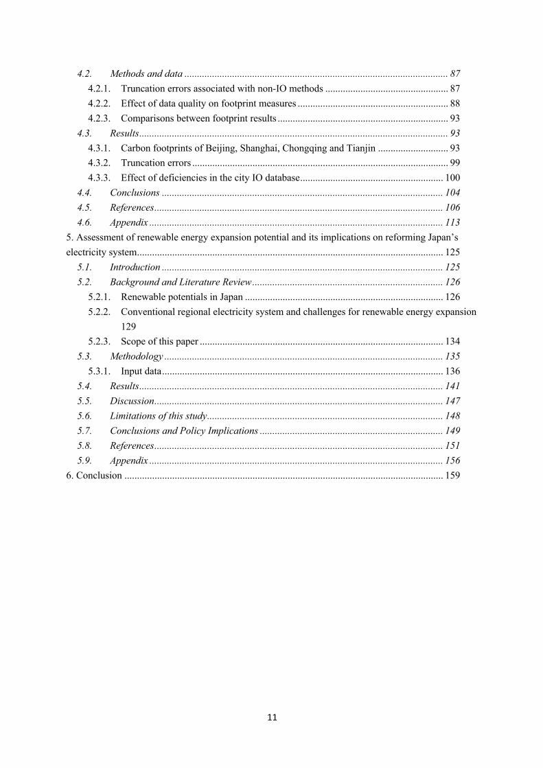
Figure 1. Schematic flows of data compilation and calculation in the Japan IELab.

2.2.2. Root table and initial estimate

As with other members of the IELab family, such as the Australia, Indonesia and China IELabs, the

Japan IELab requires a root classification and database to build sub-national MRIO tables (Geschke

and Hadjikakou 2017). To accomplish this, a city-level “root table” with detailed sectors is developed

first. The root table is compiled by disaggregating the Japan IO table to provide as many sectoral and

regional options as possible so that users can flexibly choose the sectors and regions in line with their

various research needs.

2.2.3. Creating the root table

In developing the root table, we disaggregated the most up-to-date version of the Japanese IO table

(2011), which covers one region (national) and 518 ×397 sectors by commodities (MIC 2015), into a

city-level MRIO table with sectors populated with as much detailed government-provided sectoral data

as possible. Here, we used labor survey data from the Economic Census for Business Activity (ECBA),

which distinguishes 1,615 sectors (Stat 2014). In the disaggregation process, we first identified sectors

that are covered in the 518 commodities data but not covered in the 397 commodities data, and visa

Root table(1894 cities x 4266 sectors)

National IOTPref. level IOTCity level IOTExtended IOTPref. accountsNational accountsFreight flow by 47 pref.Crop stat by citiesVegetable trade by 10 regionsFishery stat by 39 pref.

Base table(Customized table

for analysis)

Automated datastandardization

Reconciliation

Industrial stat by 47 pref.Industrial stat by cities9 regions-MRIOHousehold surveyNational household statGross Income by sector (pref. & city)Revenue (service, hospital, construction, school, wholesale, retail sectors)

Optimization

Data feed for satellite account

With selected sectors and regions for a analysis

National IOTLabour survey

Data feed for constraints

GHGs, Energy, water etc

Initial Estimate

23

verse. We then disaggregated the 518 × 397 commodities data into 522 sectors to construct a 522 ×

522 IO table using a concordance matrix (for details of the concordance method, see Lenzen et al. 2012).

The concordance method was then applied to further disaggregate the 522 sectors using domestic

production data with 3,298 sectors. The domestic production data (commodity data) were extracted

from the supplementary data provided on the Japan IO tables website maintained by the Ministry of

Internal Affairs and Communications (MIC) (MIC 2015). The mapping between the row and column

vectors of the 518 × 397 commodities matrix and the domestic production data was conducted using

the classifications described in the domestic production data sheet (MIC 2015). Since the 3,298 sectors

do not include scrap iron and non-ferrous metal scrap, the 3,298 sectors were further disaggregated into

3,300 sectors using the 522 sectors matrix that includes scrap iron and non-ferrous metal scrap. At this

point, the table remains a national-level table.

We then changed the resolution of the table from national to city level using labor survey statistics. The

labor survey contains highly detailed information on the number of workers (persons engaged in

establishments) in 544 sectors in 1,894 cities (𝐋!"), as well as the number of workers in 1,615 sectors

at the subregional level (47 prefectures) (𝐋#$) as indicated in the 2012 census data (Stat 2014). The

industrial classification of the labor survey and the IO tables are both based on the Japan Standard

Industrial Classification (JSIC) in the establishment sectors (MIC/METI 2014; MIC 2016a). Although

the labor survey classifies by industry and the IO table is by commodity, the ECBA data is one of the

key basic information sources to be used in constructing the official Japan 2011 IO tables published by

MIC (Tanaka 2016).

To make a city-level root table, we took into account different functions between headquarters and

establishments that produce and supply goods and services. The goods and services required for

headquarters is for central planning and execution, not for production. While most of the subregional

(prefecture) level IO tables do not include a sector of headquarters, the intermediate demand of the

Tokyo IO table has a sector of headquarters apart from sectors that produce goods and services

24

(Hasegawa 2012; Statistics of Tokyo 2011a). In case of the labour survey, the data as of 2012 includes

establishments engaged in administrative or ancillary economic activities by sector by city, as well as

establishments engaged in economic activities of goods and services (MIC 2014a). In order to

differentiate commodity flows at headquarters from that at goods and services producers in our

disaggregation process, we regarded the number of workers engaged in administrative or ancillary

economic activities as that at headquarters. The number was weighted using a ratio of the Tokyo’s

intermediate demand of headquarters to the total intermediate demand by sector. Although we did not

include a sector of headquarters in our root table, through this process, we adjusted a commodity flow

to a city with headquarters and to a city with establishments that produce goods and services.

Next, based on the JSIC categories, we prepared the sectoral concordance matrix 𝐌"$ (r: 544 sectors,

s: 1,615 sectors) of the labor survey and the IO table to sectorally disaggregate the regionally detailed

data 𝐋!" to produce 𝐋!$ using equation (1):

𝐋%& = 𝐋%' ×𝐌'& = 𝐋%' × &'𝐂'& × 𝐏&*× 𝟏𝑷𝒔, -)*× .𝐂'& × 𝐏&*/0 (1)

where 𝐂"𝒔 (544 × 1615) is the sectoral concordance for the labor data; and 𝐩$2 = ∑ 𝐋#$,-./*, is a proxy

vector for normalising the concordance 𝐂"$. We then built a table of 𝐋!$ consisting of 1,894 cities ×

1,615 sectors.

Then, we disaggregated the labor data (1,894 cities, 1,615 sectors) into further detailed sectors using

the aforementioned disaggregated IO table (national level, 3,300 × 3,300 sectors). The labor data were

disaggregated from 1,615 sectors into 4,266 sectors by identifying unique classifications in the 1,615

sectors that are not included in the 3,300 sectors and using a concordance matrix. At this stage, we

simply disaggregate the IO table into a matrix containing 1,894 cities and 4,266 sectors; the matrix does

not here include the inter-regional trade between sub-national regions (cities). (Estimation of inter-

regional trade is described in section 2.2.2.)

25

The root table of each city in the Japan IELab consists of a supply-use table, expressed in producer’s

price, containing information on intermediate transactions, 18 final demand categories, one export type,

and 11 value added categories (see the details in Supplementary Information (SI).1).

2.2.4. Initial estimate of MRIO with the non-survey method

One of the issues in developing MRIO tables is the difficulty in assessing inter-regional trade

coefficients (Hagiwara 2012; Hasegawa et al. 2015; Miyagi et al. 2003; Yamada 2011). This is in part

due to the lack of reliable survey data for trade statistics between countries or cities. Many researchers

have thus used non-survey methods for inter-regional trade estimation and found that the non-survey

method is a reasonable alternative approach for estimating inter-regional trade (Sargento, Nogueira

Ramos, and Hewings 2012). In most studies using MRIO tables for Japan, hybrid non-survey methods

have been applied for the construction of the tables. Cross-prefecture commodity flows are estimated

by using a non-survey method and survey data such as domestic net freight flows published by the

Ministry of Land, Infrastructure, Transport and Tourism (MLIT), production data from the Ministry of

Economy, Trade and Industry (METI), and employee commuting flows and communication traffic data

(Hagiwara 2012; Ishikawa and Miyagi 2003; Miyagi et al. 2003). On the other hand, Yamada (2011)

employs a gravity-RAS method to estimate commodity flows across regions.

In the Japan IELab, to build a customized sub-national MRIO table, we also used a regionalization

technique (a non-survey method ) (Oosterhaven, Piek, and Stelder 2005; Sargento et al. 2012). The

infrastructure of the IELab contains 11 different types of non-survey methods that can estimate inter-

regional transactions and map the data against the root classification (see Lenzen et al. (2017) for the

details of each method). Users can choose different non-survey methods depending on the kind of inter-

regional trade estimation that is required for analysis. In this paper, we use Flegg's location quotient

(FLQ) to estimate the regional input coefficients. According to an analysis conducted by Bonfiglio and

Chelli (2008), the FLQ regionalization technique reproduces multipliers more accurately, generates

more stable simulation errors and more effectively minimizes over- and under-estimate impacts

compared to other location quotient techniques.

26

2.3. Data feed constraints and reconciliation with optimization

2.3.1. Data feed constraints

We next integrated additional data sources into the initial estimate as constraints for optimization in

order to enhance the accuracy and reliability of the table. Unique to the Japan IELab (as compared to

others in the IELab family) is its integration of over 145 types of constraints (a total of 46,771

constraints for the 2011 base year tables) (See SI.2 for the details). These data are collected from the

official websites of the Japanese government.

The census of economic activity provided by Statistics Japan contains income data for the various

sectors by prefecture and city for 2012 and 2014 (Stat, 2014). Industry statistics published by METI

cover prefecture-level and city-level industrial production up to 2016 (METI, 2016). Prefecture and city

IO are provided by prefecture and city governments. Household survey data (family income and

expenditure survey) are provided by Statistics Japan (Stat, 2018) up to 2018.

Although regional transaction flows are calculated using a non-survey approach, we use survey data

such as domestic net freight flows and household surveys as supplementary data. Depending on the

features of the data, different types of constraints, including point, summation and ratio constraints, are

constructed and applied (Wang et al. 2017). For example, we use the ratio of domestic net freight flow

to the initial estimate to construct a ratio constraint that imposes defined proportions on the matrix

elements of the initial estimate. The reasoning here is that domestic net freight flow is a physical

quantity and the data is seasonal (MLIT 2017).

As another example, although the prefecture IO and city IO tables used for constraints in each regional

matrix include intermediate and final demand, we incorporate, as a supplement, household and

consumption survey data into the household sector of final demand as a point constraint. Japan’s

household survey indicating annual expenditure per household targets 9,000 households in 168 cities

(MIC 2018); the national consumption survey covers 56,400 households in the country’s 47 prefectures

(MIC 2014b). We assume that the consumption patterns in cities within a region (prefecture) are similar.

27

Therefore, we multiply the household survey data and national consumption survey data by the number

of households in a city, then apply the result as a household sector constraint.

We also use thermal power generation (coal-fired, oil-fired and gas-fired) data (METI 2015) to create

ratio constraints by city so that fuel inputs are assigned to those cities where electricity power is actually

generated. Japan has ten large regional electric utilities consisting of a headquarters and multiple power

generation facilities. While the monetary transactions of the electric power companies take place at

company headquarters, the use of fuel inputs occurs at the electricity generating facilities. We thus use

a thermal power generation (kW) ratio constraint to direct the fuel inputs to be consumed in the power

generation facilities and not at a company headquarters. This kind of adjustment is an important factor

in building a city-level MRIO table, but would be less critical in regional level analysis such as at the

prefectural level. In the Japan IELab framework, users can add their own data constraints to increase

the accuracy of the data used in their customized analysis.

2.3.2. Reconciliation with optimization

As the various primary data sources used in the process are often not compatible with respect to total

value, we used the standard deviation for each data source to determine the data points to be used in the

optimization process for constructing the MRIO table (Faturay et al. 2017) and applied the generalized

iterative scaling optimization method (KRAS) developed by Lenzen, Gallego and Wood (2009). The

KRAS optimization method can balance and reconcile conflicting external information and inconsistent

data from different sources in input-output tables and social accounting matrices (SAMs) (Lenzen,

Gallego and Wood, 2009; Lenzen et al., 2012; Wiebe and Lenzen, 2016). Reconciliation is done through

the process of constructing the MRIO table. A base table (i.e., a customized MRIO table) is finally built

for users to conduct socio-economic environmental impact analysis.

28

2.4. Results

2.4.1. Features of the Japan IELab

Figure 2 shows the graphical user interface (GUI) of the Japan IELab. The interface allows users to

easily set sectoral and regional aggregation levels, specify the initial estimate method, and indicate the

data-feeds that work as constraints for optimization. The GUI can be accessed by users through the

cloud-computing platform. Users are also able to create a concordance matrix for regions and sectors

specific to their analysis and upload it to the database. Furthermore, users can select the years that they

wish to analyze, from 2005 to the most recent year available (through 2016 as of February 2019).

Figure 2. Graphical user interface of the Japan IELab, which sets sectoral and regional aggregation level,

non-survey method of initial estimate, and data-feeds as optimization constraints.

2.4.2. Case study 1: Building a prefecture-level MRIO

As a case study to demonstrate the data-building flexibility of the Japan IELab, we built a prefecture-

level MRIO table. Twenty-four sectors were selected from the root classification (4,266 sectors) (see

the sector list in SI.3). The resulting MRIO table, with 47 prefectures and 24 sectors, is visualized as a

heatmap in Figure 3. The transactions of all 47 prefectures, including inter-regional transactions among

prefectures, are shown. The diagonal matrix on the right-hand side shows the inter-industry transactions

29

within a prefecture; the matrices between the diagonals indicate the inter-regional transactions between

regions. If the amount of a particular intermediate good is large in a given region, the heatmap indicates

it in red. Accordingly, the heatmap shows Tokyo prefecture, which locates the capital city of Japan,

with the highest transaction levels among all the prefectures. The inter-regional transactions in 47

regions are shown in the area outside of the diagonal blocks of the matrix. The column vectors of the

Tokyo region, for instance, indicate the transfer of commodities produced in Tokyo to other prefectures

(46 regions), while the row vectors indicate the commodities transferred from other regions to Tokyo

(green square matrix outside the diagonal blocks in Figure 3).

Figure 3. Heatmap of an MRIO table for 47 prefectures and 24 sectors (above)

From the intermediate matrix in the MRIO table (Figure 3), we constructed a bar graph showing the

monetary value of inputs to each sector by prefecture and checked whether the industrial activity of a

prefecture indicates its economic scale (Figure 4). The intermediate matrix expresses the flows of

commodities that are produced and consumed in the process of production of goods across cities. Figure

4 indicates that Tokyo has the highest output levels, especially in the service sector, which includes

financial intermediation, retail trade, education and health, and information and communication. In

Aichi prefecture, which has the highest production of manufactured products, the manufacture of

transport equipment has the greatest share of the intermediate goods produced in the prefecture. Aichi

30

Prefecture is the largest industrial district for car manufacture in Japan. The headquarters of Toyota

Motor Corporation is also located in the region. Such results offer evidence that the MRIO tables created

from the Japan IELab effectively capture the economic features of the individual prefectures.

Figure 4. Estimated intermediate outputs by 24 sectors for each 47 prefecture

2.4.3. Diagnostic test in case study 1

As a diagnostic test of the base table (the 47 prefectures, 24 sectors MRIO table) built for case study 1,

a rocket plot of the 2011 constraint values of each of the data points against the MRIO table values was

constructed (see Figure 5). In all, 46,771 constraint data points were compared to the MRIO values. The

average standard error was 200%. As can be seen in the figure, the larger constraint values tend to

adhere more closely to the MRIO values.

31

Figure 5. Rocket plot for year 2011 base year MRIO table and constraints

Next, we tested the inter-regional transactions between regions (prefectures). Figure 6 shows the results

of plotting the domestic net freight flow data provided by the MLIT against the inter-regional

transaction data of the MRIO used in the case study. As described in section 2.3.1, domestic net freight

flow is a physical quantity and is seasonal in nature. Because of this, the logged data are not generally

compatible with the monetary value of the MRIO. However, the trends shown in Figure 6 indicate that

the inter-regional transaction flow in the MRIO in nine aggregated sectors (Agriculture and Fishing;

Food & Beverages; Wood and Paper; Chemical Product; Plastic and Rubber Products; Iron and Steel,

32

Metal Products; Machinery; Electrical Components & Machinery; and Transport Equipment) is in

analogue with the trend of the volume traded through freight transport from one region to another.

Figure 6. Inter-regional transactions of the MRIO against the domestic net freight flow data.

As cited in the introduction, Hasegawa et al. (2015) have built a 47-region MRIO for 2005 using a nine-

region MRIO table (METI 2010), a national IO table (MIC 2016a) and prefecture IO tables published

by the governments of the 47 prefectures. Our Japan IELab MRIO reflects additional regional statistics,

including prefecture industrial statistics surveys, prefecture accounts and prefecture economic census

results as well as the statistics used in Hasegawa’s MRIO. We also built an MRIO for 2005 for

comparison with the MRIO by Hasegawa et al. (2015). In terms of the magnitude of the regional

economy, overall trade is similar; however, there is a discrepancy for each of the individual data points.

33

These differences stem from the additional data that we incorporate into our MRIO tables. Details on

the comparison are given in SI.4.

2.4.4. Case study 2: Building a city-level MRIO

A second case study demonstrating the flexibility of the Japan IELab involves a city-level MRIO table

focusing on 69 cities in Aichi prefecture. Aichi prefecture is composed of a prefectural capital city

(Nagoya city) consisting of 16 districts, 37 cities and 16 villages. We created an MRIO table with 115

regions, including the 69 districts, cities and villages in Aichi prefecture, and the other 46 prefectures.

We aggregated the 4,266 sectors into 24 sectors focused on manufacturing activities, as in case study 1.

Aichi prefecture is home to the headquarters of Toyota Motor Corporation (maker of Toyota

automobiles) and Denso Corporation (a major car parts supplier). Toyota Motor Company was the

largest global producer of automobiles in 2016 (OICA 2016), while Denso was the world’s second

largest global supplier of automotive parts according to sales in 2017 (Federal-Mogul 2018). Overall,

14% of all manufacturing shipments in Japan are generated from Aichi prefecture, while 40% of all

Japanese-manufactured transport equipment is shipped from there (METI 2016). (The location of Aichi

prefecture in Japan is shown in SI.5.)

Figure 7 shows intermediate demand production including inter-regional transactions by sector for each

city in Aichi prefecture. The values are derived from the intermediate matrix of the obtained MRIO

table. Nagoya city, with 16 assembly districts and a population of 2.6 million (30% of the prefecture’s

total population), shows the highest output levels, especially in the financial intermediate and service

sectors. Furthermore, output in the electricity sector in district 2 (Naka-ku) in Nagoya city is high

relative to the other cities in the prefecture. This is surely related to the presence of the headquarters of

Chubu Electric Power Co., Inc., one of the largest electrical utility companies in Japan that operates

electricity generation, distribution and transmission. Chubu Electric Power generates 13% (the second

largest power generation total) and distributes 16% (the second largest power distribution) of Japan’s

electricity, supplying an area covering most of five prefectures (METI 2017). As mentioned in section

34

2.3.1, fuel inputs for the electric power generation sector are adjusted by applying a constraint ensuring

that the fuel inputs are directed to the cities where the electricity generating facilities are located.

Toyota city (City 27), with the prefecture’s second largest population (0.42 million), shows a high level

of transport equipment outputs. Kariya city (City 26), home to Denso, is also shown here to produce a

large volume of transport equipment. Tokai city (City 37), where Japan’s largest iron and steel industry

(METI 2016) is located, has high outputs of metal products. These matches between the known

economic features of the cities and the MRIO table results provide further evidence of the effectiveness

of the Japan IELab.

For the base table in this case study, as we mentioned above, we first distribute the economic values

and estimate the inter-regional transaction values of each sector in each city using the labor survey and

a non-survey method for an initial estimate. We then enhance the data quality with the constraints.

While the base table represents the economic values of each city in each sector such as power generation

and transport equipment, users of the Japan IELab can improve the reliability of the MRIO table at the

city level by adding more city-level constraints in order to conduct a more detailed analysis.

Figure 7. Estimated intermediate outputs by 24 sectors for each city in Aichi prefecture

35

2.4.5. Diagnostic test in case study 2

As a diagnostic test for inter-regional trade at the city level, Figure 8 shows a plot of the total value of

inter-city materials flows (iron, steel and metal products) against the total value of transport equipment

at the city level in Aichi prefecture. As Figure 8 indicates, the cities with the higher values of transport

equipment output such as Toyota and Kariya city are shown to have the highest volume of iron, steel

and metal inputs. Moreover, the plot of the (logged) transport output values against the (logged) input

values of iron, steel and metal products necessary is linear. The standard error of the logged data ranges

from 0.5 to 0.2.

Figure 8. Rocket plot for transport equipment and its inter-regional inputs of iron, steel and metal

products

36

2.5. Discussion

As described, Japan IELab is a cloud-computing platform that enables the flexible and timely

compilation of Japanese MRIO tables. Importantly, it provides regional supply-chain data for

sustainability footprint management at the city level. As demonstrated by a number of existing input-

output analyses (Owen et al. 2016; Tarne, Lehmann, and Finkbeiner 2018; Tukker et al. 2016), MRIO

tables created with the Japan IELab allow the identification of environmental hotspots within regional

supply-chains.

Flexibility in sector selection in building an MRIO facilitates life-cycle assessment (LCA) at the product

and institutional level. Today, businesses need to consider issues of sustainability management and take

responsibility for the environmental and social impact of the products and services they provide, in

alignment with international standards and certificates of sustainability management (Balkau, Gemechu,

and Sonnemann 2015; Nikolaou, Tsalis, and Evangelinos 2019). By using LCAs, businesses can review

their sustainable performance and focus their efforts to reduce environmental burdens and improve the

economic and social value of their business as they examine the value chains of their products

(Sonnemann et al. 2015).

The Japan-IELab also makes possible the efficient updating of LCA data. For example, the latest version

of the national-level IO table published by the Japanese government is for 2015. The data seem out of

date for any current application. The Japan IELab allows easy updating of the IO table to the most recent

year, reflecting the economic changes from 2011 as expressed in statistics via the data-feeds process.

This clearly enhances the reliability of the input-output LCA.

The Japan IELab also overcomes the aggregation errors of a hybrid LCA. It covers 4,266 sectors at the

municipal level (1,894 cities). Although Japan’s LCA software has been developed by the Life Cycle

Assessment Society of Japan (JLCA) and the National Institute of Advanced Industrial Science and

Technology (AIST) (JEMAI, 2015), and Japan’s input-output LCA data have been assembled by NIES

(Nansai et al. 2012; Nansai, Moriguchi, and Tohno 2003), these are databases for LCA at the national

37

level. The novelty of the Japan IELab is that it enables users to conduct city-level and business-level

LCA that require information on the regional features of a location. In addition, MRIO tables

constructed with the Japan IELab can be augmented by a process-based LCA database or available data

from additional sources to increase data reliability.

Another promising application of the Japan IELab is in disaster impact management that considers

regional supply-chains. The Great East Japan Earthquake of 2011 directly and indirectly affected

suppliers and customers of disaster-stricken firms due to the disruption of upstream and downstream

supply chains (Okiyama, Tokunaga, and Akune 2012; Tokunaga and Okiyama 2017). To adequately

respond to such disasters and the economy-wide shocks that they produce, it is crucial for researchers

and policymakers to assess in a timely manner the impact of these external shocks on critical supply-

chains. Such assessments can be made using a high-resolution MRIO system that provides information

on transactions between the various sectors of the economy. Because the impact of a disaster on supply-

chains will differ among the affected regions and localities, detailed data on supply-chains at the local

level is required in order to assess the impacts of local-level disasters on the nation as a whole as well

as on local communities (Carvalho et al. 2014; Kajitani and Tatano 2014; Tokui, Kawasaki, and

Tsutomu 2015). Insofar as a region is likely to consist of cities with distinctly different economic

features, such features can be reflected in the Japan IELab database.

As mentioned earlier, the Japan IELab also offers time-series data from 2005 to the most recent year by

including officially available, up-to-date data sources in the city-level MRIO database. The data of the

Japan IELab are easily updated. Newly published government data can be input by users through the

cloud infrastructure. Researchers, policy-makers and business can also collaborate to enhance the

reliability and accuracy of the database by adding available data into the IELab database as constraints.

For instance, inter-regional transaction data are currently estimated using non-survey methods and

freight trade flow data. However, in the future, researchers and businesses can collaborate to disclose

or report inter-regional transaction data to trace more accurately the transaction flows between cities.

At the same time, technology developments such as smart meters and digital logistics can be used to

38

help governments and researchers collect energy supply and demand data at the household level and

accumulate freight trade flow data at the city level. If such data can be collected using information

technology (IT) and a systematic framework, the data can be readily incorporated into the Japan IELab

so that inter-regional transactions can be estimated more precisely.

Despite all of its capabilities, the Japan IELab is not without limitations. One of the limitations of the

Japan IELab in its current form is that it can only be used to assess economic, social and environmental

effects in Japan. However, actions, events and conditions in Japan affect other countries (and vice versa).

Therefore, as a next step, the Japan IELab needs to be linked to a global database so that global supply-

chains can be analyzed. This would allow, for instance, an analysis of how production of a specific

product or the consumption of a specific good in one city in Japan affects the economy and environment

of a region or city elsewhere in the world. To this end, we intend to link the Japan IELab with the IELab

family (Australia, China, Indonesia and Global) and to use this linkage to conduct a comprehensive

analysis of trade among countries.

39

2.6. References

Balkau, Fritz, Eskinder Demisse Gemechu, and Guido Sonnemann. 2015. “Life Cycle Management

Responsibilities and Procedures in the Value Chain BT - Life Cycle Management.” Pp. 195–

212 in, edited by G. Sonnemann and M. Margni. Dordrecht: Springer Netherlands.

Barrow, Martin, Carbon Trust Benedict Buckley, Gorm Kjaerbøll, Ab Electrolux Katrina Destree

Cochran, Alcatel-Lucent Isabel Bodlak, Allianz SE Arturo Cepeda, Artequimcom Ltd George

Vergoulas, Arup Nicola Paczkowski, Basf SE Will Schreiber, Best Food Forward Ricardo

Teixeira, Sara Pax, Bluehorse Associates, Dawn Rittenhouse, DuPont Chris Brown, Bernhard

Grünauer, Eon AG Corinne Reich-Weiser, Enviance Daniel Hall, ForestEthics Concepción

Jiménez-González, GlaxoSmithKline Thaddeus Owen, Herman Miller Don Adams, Keystone

Foods John Andrews, Landcare Research Maria Atkinson, Lend Lease Sustainability Solutions

Jordi Avelleneda, Mads Stensen, Maersk Line, Damco B. David Goldstein, Jorge Alberto

Plauchu Alcantara, Plauchu Consultores Nick Shufro, PricewaterhouseCoopers LLP William

Lau, Erika Kloow, TetraPak Yoshikazu Kato, The Japanese Gas Association Yutaka Yoshida,

Tokyo Gas Co, Ltd Alice Douglas, Matt Clouse, John Sottong, and Jesse Miller. 2013. Technical

Guidance for Calculating Scope 3 Emissions -Supplement to the Corporate Value Chain (Scope

3) Accounting & Reporting Standard.

Bonfiglio, A. and F. Chelli. 2008. “Assessing the Behaviour of Non-Survey Methods for Constructing

Regional Input-Output Tables through a Monte Carlo Simulation.” Economic Systems Research

20:243–58.

CAO. 2018. Prefecture Accoutns (Japanese).

Carvalho, Vasco M., David Autor, Chang-Tai Hsieh, Ulrike Malmendier, and Timothy Taylor. 2014.

“From Micro to Macro via Production Networks.”

Faturay, Futu, Manfred Lenzen, and Kunta Nugraha. 2017. “A New Sub-National Multi-Region

Input–Output Database for Indonesia.” ECONOMIC SYSTEMS RESEARCH 29(2):234–51.

Federal-Mogul. 2018. Automotive News - North America, Europe and the World Top Suppliers.

Geschke, Arne and Michalis Hadjikakou. 2017. “Virtual Laboratories and MRIO Analysis – an

Introduction.” Economic Systems Research 29(2):143–57.

40

Hagiwara, T. 2012. “Compilation of 47-Prefectures’ Interregional Input-Output Table and Its

Application (Japanese).” Kobe Univ EconRev 58.

Hasegawa, Akihiko. 2012. “Building Input-Output Table: Economy and Input-Output Table in Tokyo

- From the Field of Building Input-Output Tables (2) (Japanese).” Business Journal of PAPAIOS

20(3):205–14.

Hasegawa, Ryoji, Shigemi Kagawa, and Makiko Tsukui. 2015. “Carbon Footprint Analysis through

Constructing a Multi-Region Input–Output Table: A Case Study of Japan.” Journal of Economic

Structures 4(1).

Hitomi, KAZUMI and PONGSUN Bunditsakulchai. 2008. “Development of Multi-Regional Input

Output Table for 47 Prefectures in Japan (Japanese).” Central Res. Inst. Electric Power Ind.,

Socio-Economic Res. Center, JPN (Y07035).

Hokkaido METI. 2011. Hokkaido Intra-Regional Input Ouput Tables (Japanese).

Ishikawa, Yoshifumi and Toshihiko Miyagi. 2003. “Analysis of the Input-Output Structure Using

Multi-Prefectural Input-Output Table of Japan (Japanese).” Stud Reg Sci 34(1):139–152.

Kajitani, Yoshio and Hirokazu Tatano. 2014. “ESTIMATION OF PRODUCTION CAPACITY LOSS

RATE AFTER THE GREAT EAST JAPAN EARTHQUAKE AND TSUNAMI IN 2011.”

Economic Systems Research 26(1):13–38.

KGM. 2018. “EORA Database.” Retrieved (http://worldmrio.com/).

Lenzen, Manfred, Blanca Gallego, and Richard Wood. 2009. “MATRIX BALANCING UNDER

CONFLICTING INFORMATION MATRIX BALANCING UNDER CONFLICTING

INFORMATION.” Economic Systems Research.

Lenzen, Manfred, Arne Geschke, Arunima Malik, Jacob Fry, Joe Lane, Thomas Wiedmann, Steven

Kenway, Khanh Hoang, and Andrew Cadogan-Cowper. 2017. “New Multi-Regional Input–

Output Databases for Australia – Enabling Timely and Flexible Regional Analysis New Multi-

Regional Input–Output Databases for Australia – Enabling Timely and Flexible Regional

Analysis.” ECONOMIC SYSTEMS RESEARCH 29(2):275–95.

Lenzen, Manfred, Arne Geschke, Thomas Wiedmann, Joe Lane, Neal Anderson, Timothy Baynes,

John Boland, Peter Daniels, Christopher Dey, Jacob Fry, Michalis Hadjikakou, Steven Kenway,

41

Arunima Malik, Daniel Moran, Joy Murray, Stuart Nettleton, Lavinia Poruschi, Christian

Reynolds, Hazel Rowley, Julien Ugon, Dean Webb, and James West. 2014. “Compiling and

Using Input–Output Frameworks through Collaborative Virtual Laboratories.”

Lenzen, Manfred, Keiichiro Kanemoto, Daniel Moran, and Arne Geschke. 2012. “Mapping the

Structure of the World Economy.” Environmental Science & Technology.

Lin, Jianyi, Yuanchao Hu, Xiaofeng Zhao, Longyu Shi, and Jiefeng Kang. 2017. “Developing a City-

Centric Global Multiregional Input-Output Model (CCG-MRIO) to Evaluate Urban Carbon

Footprints.” Energy Policy 108:460–66.

Lombardi, Mariarosaria, Elisabetta Laiola, Caterina Tricase, and Roberto Rana. 2017. “Assessing the

Urban Carbon Footprint: An Overview.” Environmental Impact Assessment Review 66:43–52.

Long, Yin and Yoshikuni Yoshida. 2018. “Quantifying City-Scale Emission Responsibility Based on

Input-Output Analysis – Insight from Tokyo, Japan.” Applied Energy 218:349–60.

MAFF. 2017a. Agricultural Production by City (Japanese).

MAFF. 2017b. Fisheries Yield (Japanese).

MAFF. 2017c. Fruit and Vegetables Wholesale Market (Japanese).

METI. 2010. Japan 2005 Multi-Regional Input Output Tables (Japanese).

METI. 2015. List of Major Thermal Power Plants in Japan and Prospects for New Establishments /

Updates.

METI. 2016. “Industry Statistics (Japanese).” Ministry of Economy, Trade and Industry.

METI. 2017. “Survey of Electric Power Statistics (Japanese).” Ministry of Economy, Trade and

Industry.

Mi, Zhifu, Yunkun Zhang, Dabo Guan, Yuli Shan, Zhu Liu, Ronggang Cong, Xiao-Chen Yuan, and

Yi-Ming Wei. 2016. “Consumption-Based Emission Accounting for Chinese Cities.” Applied

Energy 184:1073–81.

MIAC. 2018. Japan Statistical Yearbook 2018.

MIC/METI. 2014. 2012 Economic Census for Business Activity (Definitive Report): Tabulations

across Industries (Detailed Data) - Summary of Census Results.

MIC. 2014a. General Principal of Japan Standard Industrial Classification (Japanese).

42

MIC. 2014b. “National Survey of Family Income and Expenditure (Japanese).” Ministry of Internal

Affairs and Communications.

MIC. 2015. 2011 Input-Output Tables.

MIC. 2016a. “2011 Input-Output Tables for Japan.” Ministry of Internal Affairs and Communications

Japan.

MIC. 2016b. Time Series Connection Input-Output Tables (Japanese).

MIC. 2018. “Family Income and Expenditure Survey (Japanese).” Ministry of Internal Affairs and

Communications.

Miyagi, Toshihiko, Yoshifumi Ishikawa, Shohei Yuri, and Kazuyuki Tsuchiya. 2003. “Construction

of Interregional Input-Output Table at Prefecture Level Using Intra-Regional Input-Output Table

(Japanese).” Infrastruct Plan Rev 20(1):87–95.

MLIT. 2017. Net Freight Flow Census (Japanese).

Nansai, Keisuke, Yasushi Kondo, Shigemi Kagawa, Sangwon Suh, Kenichi Nakajima, Rokuta Inaba,

and Susumu Tohno. 2012. “Estimates of Embodied Global Energy and Air-Emission Intensities

of Japanese Products for Building a Japanese Input–Output Life Cycle Assessment Database

with a Global System Boundary.” Environmental Science & Technology 46(16):9146–54.

Nansai, Keisuke, Yuichi Moriguchi, and Susumu Tohno. 2003. “Compilation and Application of

Japanese Inventories for Energy Consumption and Air Pollutant Emissions Using Input−Output

Tables.” Environmental Science & Technology 37(9):2005–15.

Neirotti, Paolo, Alberto De Marco, Anna Corinna Cagliano, Giulio Mangano, and Francesco

Scorrano. 2014. “Current Trends in Smart City Initiatives: Some Stylised Facts.” Cities 38:25–

36.

Nikolaou, Ioannis E., Thomas Tsalis, and Konstantinos Evangelinos. 2019. “A LCA Technique to

Measure the Socially Business Responsible Profile: The Case of Food Industry BT - Social Life

Cycle Assessment: Case Studies from Agri and Food Sectors.” Pp. 39–57 in, edited by S. S.

Muthu. Singapore: Springer Singapore.

OICA. 2016. WORLD MOTOR VEHICLE PRODUCTION OICA Correspondents Survey.

Okiyama, Mitsuru, Suminori Tokunaga, and Yuko Akune. 2012. Multiplier Analysis on Supply

43

Chains by and Economic Ripple Effect of Reconstruction from the Great East Japan Earthquake

- Using Two Regional SAM - (Japanese).

Oosterhaven, Jan, Gerrit Piek, and Dirk Stelder. 2005. “THEORY AND PRACTICE OF UPDATING

REGIONAL VERSUS INTERREGIONAL INTERINDUSTRY TABLES.” Papers in Regional

Science 59(1):57–72.

Owen, Anne, Richard Wood, John Barrett, and Andrew Evans. 2016. “Explaining Value Chain

Differences in MRIO Databases through Structural Path Decomposition.” Economic Systems

Research 28(2):243–72.

Ramaswami, Anu, Dana Boyer, Ajay Singh Nagpure, Andrew Fang, Shelly Bogra, Bhavik Bakshi,

Elliot Cohen, and Ashish Rao-Ghorpade. 2017. “An Urban Systems Framework to Assess the

Trans-Boundary Food-Energy-Water Nexus: Implementation in Delhi, India.” Environmental

Research Letters 12(2):025008.

Ramaswami, Anu, Armistead G. Russell, Patricia J. Culligan, Karnamadakala Rahul Sharma, and

Emani Kumar. 2016. “Meta-Principles for Developing Smart, Sustainable, and Healthy Cities.”

Science 352(6288):940 LP – 943.

Sargento, Ana LM, Pedro Nogueira Ramos, and Geoffrey JD Hewings. 2012. “INTER-REGIONAL

TRADE FLOW ESTIMATION THROUGH NON-SURVEY MODELS: AN EMPIRICAL

ASSESSMENT.”

Sonnemann, Guido, Eskinder Demisse Gemechu, Arne Remmen, Jeppe Frydendal, and Allan Astrup

Jensen. 2015. “Life Cycle Management: Implementing Sustainability in Business Practice BT -

Life Cycle Management.” Pp. 7–21 in, edited by G. Sonnemann and M. Margni. Dordrecht:

Springer Netherlands.

Stat. 2014. Economic Census for Business Activity (Japanese).

Stat. 2018a. Family Income and Expenditure Survey (Japanese).

Stat. 2018b. Household Survey (Japanese).

Statistics of Tokyo. 2011a. “Structure and Characteristics of the Tokyo Input-Output Table

(Japanese).” Statistics Division, Bureau of General Affairs, Tokyo Metoropolitan Government.

Statistics of Tokyo. 2011b. Tokyo 2011 Intra-Regional Input Ouput Tables (Japanese).

44

Tanaka, Masayuki. 2016. “Compilation of 2011 Input-Output Table and Its Outline (Japanese).”

Input-Output Analysis 23(3):102–15.

Tarne, Peter, Annekatrin Lehmann, and Matthias Finkbeiner. 2018. “A Comparison of Multi-Regional

Input-Output Databases Regarding Transaction Structure and Supply Chain Analysis.” Journal

of Cleaner Production 196:1486–1500.

Tokui, Joji, Kazuyasu Kawasaki, and Miyagawa Tsutomu. 2015. “The Economic Impact of Supply

Chain Disruptions from the Great East Japan Earthquake.”

Tokunaga, Suminori and Mitsuru Okiyama. 2017. “Analysis of Supply Chain Disruptions from the

Great East Japan Earthquake in the Automotive Industry and Electronic Parts/Devices.” Pp. 95–

119 in Vol. 11.

Tukker, Arnold, Tanya Bulavskaya, Stefan Giljum, Arjan de Koning, Stephan Lutter, Moana Simas,

Konstantin Stadler, and Richard Wood. 2016. “Environmental and Resource Footprints in a

Global Context: Europe’s Structural Deficit in Resource Endowments.” Global Environmental

Change 40:171–81.

UN. 2015. “Transforming Our World: The 2030 Agenda for Sustainable Development.” General

Assembley 70 Session 16301(October):1–35.

Wang, Yafei. 2017. “An Industrial Ecology Virtual Framework for Policy Making in China.”

ECONOMIC SYSTEMS RESEARCH 29(2):252–74.

Wang, Yafei, Arne Geschke, and Manfred Lenzen. 2017. “Constructing a Time Series of Nested

Multiregion Input–Output Tables.” International Regional Science Review 40(5):476–99.

Wiebe, Kirsten S. and Manfred Lenzen. 2016. “To RAS or Not to RAS? What Is the Difference in

Outcomes in Multi-Regional Input–Output Models?” ECONOMIC SYSTEMS RESEARCH

28(3):383–402.

Wiedmann, Thomas, Harry C. Wilting, Manfred Lenzen, Stephan Lutter, and Viveka Palm. 2011.

“Quo Vadis MRIO? Methodological, Data and Institutional Requirements for Multi-Region

Input–Output Analysis.” Ecological Economics 70(11):1937–45.

Wiedmann, Thomas, Richard Wood, Jan C. Minx, Manfred Lenzen, Dabo Guan, Rocky Harris, and

Rocky Harris G. 2010. “A CARBON FOOTPRINT TIME SERIES OF THE UK – RESULTS

45

FROM A MULTI-REGION INPUT–OUTPUT MODEL A CARBON FOOTPRINT TIME

SERIES OF THE UK – RESULTS FROM A MULTI-REGION INPUT –OUTPUT MODEL.”

Wilmsen, Felix and Friederike Gesing. 2016. “The Global Protocol for Community-Scale Greenhouse

Gas Emission Inventories (GPC) – A New Passage Point on an Old Road?” ZenTra Working

Paper in Transnational Studies (68/2016).

WRI, C40, and ICLEI. 2014. Global Protocol for Community-Scale Greenhouse Gas Emission

Inventories - An Accounting and Reporting Standard for Cities.

Yamada, Matsuo. 2011. “Construction of a Multi-Regional Input-Output Table for Nagoya

Metropolitan Area, Japan Construction of a Multi-Regional Input-Output Table for Nagoya

Metropolitan Area.” Journal of Economic Structures 4:2193–2409.

Yamada, Mitsuo. 2015. “Construction of a Multi-Regional Input-Output Table for Nagoya

Metropolitan Area, Japan.” Journal of Economic Structures 4(1):11.

Zhang, Pengpeng, Lixiao Zhang, Yuan Chang, Ming Xu, Yan Hao, Sai Liang, Gengyuan Liu, Zhifeng

Yang, and Can Wang. 2019. “Food-Energy-Water (FEW) Nexus for Urban Sustainability: A

Comprehensive Review.” Resources, Conservation and Recycling 142:215–24.

46

2.7. Supplementary information

SI.1. Accounting format of the root table

Figure SI.1. shows the data structure of the root tables in the Japan IELab. The supply-use table structure

is required in order to integrate the Japan IELab into the infrastructure of the IELab family. Currently,

there exists no supply-use table for Japan, although a supply table is published by the Ministry of

Internal Affairs and Communications (MIC 2015). Therefore, while we create a use table from the Japan

IO table, in order to balance the supply-use table as a commodity-by-commodity table, we tentatively

construct the supply table by creating a diagonal table based on the total output data of the Japan IO

table2. Users of the Japan IELab can utilize the use table from the supply-use structured MRIO table to

do their analysis. Within the Japan IELab framework, in addition to the producer’s price table, nine

margin tables are contained, including wholesale trade, retail trade, railway transport, road transport,

coastal and inland water transport, harbor services, air transportation, and consigned forwarding (MIC

2015).

2 Japan provides a national intermediate demand (T) matrix that consists of commodity by commodity and is estimated by

survey data. Therefore, we are able to directly produce a technical coefficients (A) matrix with commodity by commodity

dimension by T 𝑥"^-1 (x is total output). The A matrix is more reliable than a computed A matrix based on any assumption.

47

Figure SI.1. Data structure of root tables in the Japan IELab.

Note: T is intermediate inputs; U is use; V is supply; y is final demand, including consumption

expenditure, gross fixed capital and changes in inventories; and v is value added, including gross

operating surplus and depreciation.

SI.2. List of constraints for the Japan IELab

Table SI.2 indicates the 145 types of constraints included in the Japan IELab. In total, there are 46,771

data points for the 2011 base year.

Table SI.1. List of constraints for the Japan IELab. Note: ID: Intermediate demand data; IR: Inter-

regional transaction flow data; FD: Final demand data; and VA: Value added data

Data source name Year range Regional Sectoral Constrained part Reference National Input-Output Table

2005, 2011 1 nation 517×405, 518×397

ID, FD, VA, imports, Exports

(MIC 2015) 1 type of constraint

Inter-Regional Input-Output Table

2005 9 regions 55×53 ID, FD, VA, Imports, Exports, IR

(METI 2010) 1 constraint

Economic Census (Labor survey)

2009, 2011 47 prefectures 1617 ID (Stat 2014) 1 constraint

T

v1894 regions x 11 sectors

Costal and inland water

Consigned forwarding

HarbourAir transportation

RailwayRoad

RetailWholesale

Producer’s price

Purchaser’s price

V1894 region x 4266 sectors

U1894 region

x 4266 sectors

y1894 regions x 17 sectors

48

Economic Census (Labor survey)

2009, 2011 1894 cities 591 ID (Stat 2014) 1 constraint

Hokkaido Intra-Regional Input-Output Table

2011 6 regions 33 ID, FD, VA, Imports, Exports, IR

(Hokkaido METI 2011) 1 constraint

Tokyo Intra-Regional Input-Output Table3

2011 2 regions (Tokyo, other region)

191 ID, FD, VA, Imports, Exports, IR

(Statistics of Tokyo 2011b) 1 constraint

Prefecture Input-Output Table3

2011 47 regions Varies by prefectures

ID, FD, VA, Imports, Exports

47 Prefecture government websites 47 constraints

City Input-Output Table

2005, 2010, 2011, 2012 or 2014

22 cities Varies by cities


City government websites 22 contraints

Time series connection Input-Output Table

2011-2015 1 nation 516×395, 516×394


(MIC 2016b) 1 constraint

Prefecture Accounts

2006-2015 47 prefectures

23 U, V, FD, VA (CAO 2018) 1 constraint

National Accounts

1994-2016 1 nation 23 U, V, FD, VA (CAO 2018) 1 constraint

City Accounts 2006-2016 1243 cities Varies by cities

ID, FD, VA, X City government websites 47 constraints

Household Expenditure Survey

2002-2017 47 prefectures 512 FD (Stat 2018b) 1 constraint

Family Income and Expenditure Survey

2014 47 prefectures 100 FD (Stat 2018a) 1 constraint

Agricultural Crop statistics survey

2014 2012-2017

1894 cities 17 ID (Crops, vegetables sector)

(MAFF 2017a) 1 constraint

Agricultural Vegetable Trade flow

2014 10 regions 15 IR (Vegetable sector)

(MAFF 2017c) 1 constraint

Fishery statistics 2009-2016 47 prefectures 97 ID (Fishery sector) (MAFF 2017b) 1 constraint

Prefecture Industrial statistics survey

2011-2014 47 prefectures 545 ID (Industry sector)


City Industrial statistics survey

2011-2014 1894 cities 24 ID (Industry sector)


Economic Census Income (School)

2012, 2016 47 prefectures 8 ID (School sector) (Stat 2014) 1 constraint

Economic Census Income (Sales)

2012, 2016 47 prefectures, 20 designated cities

166 ID (Whole sales and retails sector)

(Stat 2014) 1 constraint

Economic Census Income (Sales)

2012, 2016 1009 cities 49 ID (Whole sales and retails sector)


Economic Census Income (Construction)

2012, 2016 47 prefectures 20 ID (Construction sector)


3 Tokyo IO tables and Tokyo Intra-Regional IO tables have a sector of headquarters, as well as sectors of goods and services.

Therefore, we allocated the sector of headquarters to the sectors of goods and services using a concordance matrix.

49

Economic Census Income (Hospital)

2012, 2016 47 prefectures 32 ID (Hospital sector)


Economic Census Income (all sectors) Establishments

2012, 2016 47 prefectures 95 ID (all sectors) (Stat 2014) 1 constraint

Economic Census Income (all sectors) Establishments

2012, 2016 1894 cities 21 ID (all sectors) (Stat 2014) 1 constraint

Economic Census Income (all sectors) Enterprises

2012, 2016 47 prefectures 95 ID (all sectors) (Stat 2014) 1 constraint

Economic Census Income (all sectors) Enterprises

2012, 2016 1894 cities 21 ID (all sectors) (Stat 2014) 1 constraint

Economic Census Income (Service sectors)

2012, 2016 47 prefectures

251, 211 ID (Service sectors)


Economic Census Income (Service sectors)

2012, 2016 789 cities 22 ID (Service sectors)


Logistic Census (Inter-prefecture)

2005, 2010, 2015

47 prefectures 85 IR, Imports, Exports

(MLIT 2017) 1 constraint

Thermal power generation

2015 1894 cities Coal, oil and gas

IR (METI 2015) 1 constraint

50

SI .3. Sectors for the case study MRIO tables

Table SI.2. lists the sectors used for the MRIO tables built for case studies 1 and 2. The selection of

sectors is based on the EORA database (KGM 2018) and the industrial categories of the Economic

Census for Business Activity (Stat 2014)

Table SI.2. List of 24 sectors for the MRIO tables built for case studies 1 and 2

Agriculture and Fishing

Mining and Quarrying

Construction

Food & Beverages

Textiles and Wearing Apparel

Wood and Paper

Chemical Product

Petroleum and Coal Products

Plastic and Rubber Products

Non-Metallic Mineral Products

Iron and Steel, Metal Products

Machinery

Electrical Components & Machinery

Transport Equipment

Other Manufacturing

Electricity

Gas and Water

Information and Communications

Transport and Postal Activities

Wholesale & Retail Trade

Financial Intermediation and Business Activities

Education and Health

Other Services

Public Administration

51

SI.4. Comparison of a 47 prefecture 9 sector table by Hasegawa and one by

the Japan IELab

We built a 2005 MRIO table using the Japan IELab, and compared it to the 2005 table produced by

Hasegawa, Kagawa, and Tsukui (2015). Figure SI.2 shows the Rocket plot of the comparison. In the

figure, the data values for the various sectors and regions of the Japan IELab MRIO table are plotted

against the Hasegawa MRIO table. To simplify the comparison, we aggregated the Hasagawa table and

the Japan IELab table into nine sectors. As can be seen here, there are differences between data point

values in the two tables. This is largely due to the fact that the Japan IELab includes more data and uses

optimization methods to build the 47 region MRIO, while Hasegawa et al. did not optimize the data

incorporated into their MRIO.

Figure SI.2. Rocket plot comparison of a 47 prefecture, 9 sector table produced by Hasegawa and one

produced by the Japan IELab: the nine sectors included here are Agriculture, fishery & mining;

Manufacture; Construction; Electricity, gas & water; Wholesale & retail; Finance; Transport; Public

administration; and Service.

52

SI.5. Locational Map of Japan and Aichi Prefecture

Figure SI.3 shows a map of Japan. The dark blue color indicates larger prefecture populations. In the

lower right corner of the figure, Aichi prefecture is magnified and its four major industrial cities are

highlighted. For instance, the yellow area is Nagoya, the capital city of Aichi prefecture.

Figure SI.3. Map of Japan and Aichi prefecture

Toyota city

Tokai cityKariya city

Nagoya city

53

Chapter 3 Responsibility for Food Loss from a Regional Supply-Chain Perspective

3.1. Introduction

Food security is one of several key global issues related to sustainability (UN 2015). According to the

United Nations Food and Agriculture Organization (FAO), every year, 1.3 billion tonnes of food is

wasted or lost in supply chains, equivalent to one-third of all food produced for human consumption

(FAO, 2011). According to the FAO, food that is lost in the production, post-harvest and processing

stages is designated as ‘food loss’, whereas food that is ready for human consumption but discarded by

retailers or consumers is recorded as ‘food waste’ (FAO 2011; Gustavsson et al. 2013).

Reducing food waste and food loss generated through the whole food supply chain has become a global

requirement. One of the Sustainable Development Goals (SDGs) accepted by the 193 member states of

the United Nations aims to ensure sustainable consumption and production (SCP) patterns. The Goal

aims at “by 2030, halving per capita global food waste at the retail and consumer level, and reduce

food losses along production and supply chains, including post-harvest losses” (UN, 2015, page 22).

To confront this global challenge, the Japanese government has promoted the reduction of food waste

generated in food-related industries by introducing a recycling policy for food waste under the ‘Act on

Promotion of Recycling and Related Activities for the Treatment of Cyclical Food Resources’.

According to an estimate by the MOE (Ministry of the Environment, Japan) and the MAFF (Ministry

of Agriculture, Forestry and Fisheries), 27.75 million tonnes of food is wasted per year in Japan as of

2014 (MOE 2017). Of this, 6.21 million tonnes is edible but discarded before consumption. Of the

wasted edible food, 3.39 million tonnes are generated from food-related business, and 2.82 million

54

tonnes come from households. The Japanese government is striving to reduce the amount of wasted

edible food to achieve the SDG target (MOE 2017).

Edible food that is discarded before reaching consumers includes food loss categorized by the FAO as

food disposed of in the agricultural production stage, not only food waste discarded during distribution

and consumption (Johnson et al., 2018). In fact, as noted earlier, the SDG target ‘to ensure sustainable

SCP patterns’ includes reducing “post-harvest losses”. Therefore, Japan could also aim at reducing

food loss in the post-harvest stages of the supply chain as a contribution toward achieving the SDG

target. Reducing food loss also helps to enhance food security by increasing food self-sufficiency

(Clapp 2017). Furthermore, water, cropland, energy, and fertilizers are used for food production, so

reducing food loss provides a benefit in mitigating CO2 and nitrogen emissions, and soil degradation

through reduced use of energy and fertilizers (FAO, 2008; Gruber and Galloway, 2008; Rockström et

al., 2009; Bobbink et al., 2010; FAO, 2011; Mekonnen and Hoekstra, 2011; Kummu et al., 2012).

However, the amount of food lost at the agricultural production and post-harvest stages of the supply

chain has not been quantified in Japan. Few studies have specifically examined food loss during

agricultural production (Kimura 2013; Kodera and Isobe 2016; Engström and Carlsson-Kanyama 2004).

Policies and measures to reduce food loss have not been actively implemented. Therefore, there is

currently no concrete action or target for tackling the food loss issue in Japan. In contrast, food loss at

the agricultural production stage, categorized by the FAO as the first system boundary of food loss and

waste in the overall supply chain, is not treated as actual loss of food but as an amount of depletion

(MAFF 2007a; Kimura 2013). This means that crops disposed of in the field are counted as losses

during the delivery of food from production sites to consumers, similar to losses during transportation

and storage. In Japan, allowing food loss at the agricultural production stage is a practice supported by

the government to maintain ready access to food and to secure a sufficient stock in case of emergency

(MAFF 2007a). Its intent is to cope with surplus volumes of production incurred in good weather to

keep prices of agricultural crops constant and to stabilize the supply (MAFF, 2007a; Kurasaka et al.,

2010). The practice is called ‘field disposal’, wherein agricultural products, specifically vegetables, are

disposed of on site at the field during times of oversupply.

55

The main causes of food loss include not only oversupply caused by overproduction, but also

nonstandard products that cannot be sold in a market (Kurasaka et al., 2010). Some agricultural products

are not delivered to consumers because they do not meet market standards for acceptable size and shape

or are not of a certain quality (Mattsson 2014). If they do not meet the standards, they are not delivered.

However, issues of overproduction and nonstandard products might be resolved by increasing

communication that occurs among producers, buyers and consumers (MAFF 2007a, 2007c). Although

nonstandard products are discarded before reaching consumers, various needs and markets exist for

such agricultural products (Tsuruta et al., 2007; Tamura 2015). For instance, an Australian grocery

chain, Harris Farm Markets, has sold over 15 million kilograms of imperfect vegetables and fruit over

three years via a campaign (Harris Farm 2018; Australian Government 2017) that aims to reduce the

amount of farmers’ crops discarded at the farm and not delivered to market because they do not meet

such standards.

One measure to reduce food loss generated by not using nonstandard agricultural products and

overproduction is to reveal how much food is lost at the point of agricultural production (producer’s

responsibility), and to identify potential demand for crops that do not reach markets (consumers’

responsibility). This intended demand comes from industries that require agricultural crops to produce

their products or provide their services, such as food manufacturing, food-related business, and the

social service industry. By quantifying food loss at production sites and identifying intended markets,

producers’ and consumers’ needs can be visualized, and the distribution channels for such products can

be re-examined (Hobbs and Young 2000). A coordination of the producers’ and consumers’ needs

might help to reduce the amount of agricultural products discarded in fields.

Furthermore, enhancing and sharing information on food loss could help consumers as well as

producers to make efforts to reduce food loss. There is usually an information gap between producers

and consumers, especially related to issues such as environmental burdens (Poore and Nemecek 2018;

Grunert et al., 2014). Pollution is emitted during the production of agricultural crops and its impacts are

evident in the fields. Consumers are unaware of such pollution related to the products they purchase

56

(Zaks et al. 2009). Similar to such environmental burdens, food loss is not recognized by consumers,

although both producers and consumers bear responsibility for it. Thus, revealing the amount of food

lost and identifying both producers’ and consumers’ responsibility for that loss is the first step to

reductions. It also helps the government to set up targets and investment plans for policies and measures

to avoid overproduction (Australian Government 2017).

Footprint analysis has been widely used to fill in the information gaps about the environmental burdens

occurring throughout supply chains (Hoekstra and Wiedmann 2014; Lenzen et al. 2007; Gruber and

Galloway 2008). Multi-regional input–output (MRIO) analysis is a particularly useful approach to

quantifying the footprints of both producers and consumers across different countries or regions. In fact,

MRIO analyses are used globally to calculate the environmental, economic and social footprints of a

product or activity at the international and subnational level (Wiedmann, 2009; Lenzen et al., 2012;

Lenzen et al., 2018; Wiedmann and Lenzen, 2018). Footprints calculated using MRIO analysis track

the impacts of local consumption on the environment through the whole supply chain. For instance,

carbon footprint analysis quantifies the amount of CO2 emitted over the full life cycle of a product from

its raw materials, through manufacturing to consumption (Lenzen et al., 2004; Cu Cek et al., 2012;

Lenzen, 2013). A subnational MRIO analysis can track inter-regional trade for cities, counties or states

within a country (Hitomi and Bunditsakulchai, 2008; Zhang and Anadon, 2014; Wu and Liu, 2016;

Lenzen et al., 2018). Therefore, a footprint analysis conducted using an MRIO database can help fill in

information gaps between producers and consumers on the issue of food loss and can enhance their

mutual communication to bring about loss reductions.

Being aware of the issues described above, in this paper, we conduct a food loss analysis, aiming to

estimate the amount of food loss at the regional level in Japan. We examine food loss not only from a

production perspective (producers’ responsibility), but also from a demand-side perspective (consumers’

responsibility). To analyze consumers’ responsibility, we infer the markets for vegetables to which the

vegetables would have been delivered had they not been discarded in the field. We quantify regional

food loss footprints using a subnational MRIO database to ascertain where the food loss occurs and

57

where the agricultural products discarded in fields would presumably be delivered and consumed.

Moreover, we estimate the environmental burdens caused by agricultural production that is harvested

but not delivered to market.

This paper comprises five sections. Following the introduction, section 2 presents our methods and the

data used for estimating regional food loss and our footprint analysis. Section 3 presents the results of

our footprint assessment by identifying inter-regional supply chain relations in terms of food loss. We

conclude with a discussion in section 4.

3.2. Methods and data

3.2.1. Estimating regional food loss

The main issue hindering food loss estimation is a lack of data related to food loss. We do not know the

degree to which vegetables and fruit are discarded annually in fields. Therefore, we first collect annual

vegetable and fruit production and shipment data by production site and by crop. Those data are

published by the MAFF (MAFF 2015e, 2015c, 2015d). Then, we calculate any differences in the data

between production and shipment to estimate the amount of field disposal by region and by crop. We

assume the differences to be food loss. We collect data for 139 types of domestic vegetables and fruit

including local specialty crops by prefecture as of 2014. Then we estimate the total amount of food loss.

Japanese annual vegetable and fruit production data are estimated by multiplying crop yields per 10

acres by planted areas. Such data are collected through online and mail surveys, and complemented by

patrols and information-gathering by governmental official staff and statisticians (MAFF 2015c).

Shipping data are collected through invoices from shipping associations, and display labels that show

the quantities recorded in shipping registers.

Field disposal of agricultural products occurs mainly for vegetables such as potatoes, carrots, onions,

and white radishes since they are perishable goods produced especially through outdoor cultivation.

Yields are strongly influenced by weather. The market price fluctuates considerably along with supply

and demand (MAFF 2007b; Dixie 2005). In our analysis, we estimated food loss for 14 vegetables (out

58

of 139 types of vegetables and fruit) for 47 prefectures4. These include white radishes, carrots, potatoes,

taro, Chinese cabbage, cabbage, spinach, lettuce, Japanese leeks, onions, cucumbers, eggplants,

tomatoes, and green peppers. These make up 60% of the total annual production in Japan (MAFF 2015e).

Furthermore, these vegetables are designated by the Japanese government as vegetables that are traded

nationwide and annually consumed in large quantities (MAFF 2015e). The Japanese government has

strived to stabilize the price of these 14 vegetables by supporting the formation and maintenance of

their production sites under a law called ‘Act on Stabilization of Production and Shipment of Vegetables’

(ALIC 2017).

3.2.2. Subnational-level MRIO addressing the food supply system

To identify the amount of agricultural products discarded in the field, where this occurs, and how much

are otherwise sold and consumed, we analyze the supply chain of agricultural products ending up

discarded in fields by constructing a Japanese subnational MRIO table including 47 prefectures and 19

sectors. The MRIO table is constructed using the same framework used by the Australian MRIO

database compiled by Lenzen et al. (2014). We disaggregate Japan’s input-output table (one region

(national), 518 ×397 sectors) (MIC 2015) using labor survey data from the Economic Census for

Business Activity (Stat 2014a) to make an MRIO table with 47 regions and 19 sectors. The 19 sectors

consist of the 14 vegetables, other agricultural products including fruit and vegetables besides those 14,

three major stakeholders of food supply chains (food manufacturing, food-related business and the

social service industry, and the restaurant and food service industry), and other remaining sectors (the

classifications of these sectors are listed in Appendix 1). The main aim of our analysis is to examine the

supply chain of the 14 subject vegetables. Thus, we examine their production sites, their demand by

sector, which indicates where they are intended to be used, and their final demand, which indicates

where they are intended to be finally consumed. We identify sectors that use vegetables as inputs for

their production, and then classify them into eighteen food-related sectors. Other remaining sectors are

aggregated as not being related to a food business. We do not examine the food loss of vegetables and

4 Japan has a two-tier local authority system; prefectures as regional governmental units and municipalities (cities) as the basic

local governmental unit. There are 47 prefectures, constituting the first level of jurisdiction and administrative division.

59

fruit other than the 14 types, because as described in section 2.1, we focus on the footprints of food loss

for those officially designated vegetables. In addition, the trade flow of vegetables and fruit other than

those 14 is not clear and they are not distributed countrywide.

In order to construct a subnational inter-regional MRIO table, we estimated inter-regional transactions

using a non-survey method because of the lack of reliable survey data underpinning inter-regional trade

coefficients (Miyagi et al., 2003; Yamada, 2011; Hasegawa et al., 2011; Hagiwara, 2012). Many

researchers have used non-survey methods for inter-regional trade estimation, finding this to be a useful

alternative in the absence of data (Sargento, Nogueira Ramos, and Hewings, 2012). For our analysis,

we use a CHARM variant, which is a combination of the commodity-based method and the cross-

hauling method (Kronenberg 2009; Többen and Kronenberg 2015). In contrast to a single-country

input-output table, an MRIO table includes trade transactions between multi-regions, as described by

Hasegawa et al. (2011) and Lenzen et al. (2017) for a subnational MRIO table, and Lenzen et al. (2013)

and Hiramatsu et al (2016) for a global MRIO table. Our subnational MRIO table includes intermediate

demand (19 sectors, 47 prefectures), final demand such as household consumption, government

spending and inventory (18 sectors5, 47 prefectures), value-added (11 sectors6, 47 prefectures) and

exports (1 sectors, 1 rest-of-world region). To increase the reliability of entries regarding inter-regional

trade of vegetables described in our MRIO table, we incorporated agricultural trade data from the

‘Vegetable wholesale market research report’ (MAFF 2015b). These market data cover 80% of the

annual transaction volume of the total vegetable wholesale market (MAFF 2015b). Using these data,

we can trace how many tonnes of the 14 types of vegetables are delivered from production sites to

markets at the prefectural level. In addition, we use agricultural wholesale market data (MAFF 2015a)

that indicate how much of each are traded in the wholesale market in quantities (tonnes) and by

monetary value (Japanese Yen) at the prefecture level.

5 The 18 sectors in final demand are the same as the sectors in Japan’s final demand input output table 2011. 6 The 11 sectors in value added are the same as the sectors in Japan’s value added input output table 2011.

60

3.2.3. Subnational-level MRIO calculations

Using the 47-region 19-sector MRIO table including the 14 chosen vegetables (Figure 1), the

agricultural food supply chain network can be enumerated using the Leontief demand-pull model

(Leontief 1970). In this model, the amount of production is determined by final demand. For instance,

agricultural commodities are distributed to markets where demand exists.

Using the Leontief inverse matrix, we calculate food loss footprints for the 14 vegetables. First, we

calculated multipliers m = 𝐪 × (𝐈 − 𝐀))* , where the 1× 𝑁 matrix 𝐪 = 𝐐𝐱=)* holds the food loss

coefficients in units of tonne/million yen (t/¥), with Q being a 1× 𝑁 food loss matrix and 𝐱 being the

1× 𝑁 total output. In our work N = 893, the product of 19 sectors by 47 regions. The N× 𝑁 matrix𝐀 =

𝐓𝐱=)* holds economic input coefficients, derived by by dividing input-output transactions Tij by total

output xj. (𝐈 − 𝐀))* =: 𝐋 is the Leontief inverse. The multiplier captures the ripple effects of food loss

starting with the consumption of the 14 vegetables and progressing over the entire product supply chain.

Supply chain coverage is aided by the Japanese subnational MRIO database, as it includes all monetary

transactions occurring in Japan. We post-multiply the multiplier by final demand (y) to calculate

consumers' responsibility for food loss. Instead of applying a matrix product (my or qLy), we use an

element-wise product (m#y or qL#y) that retains the N region-sector detail.

We calculated the consumers’ responsibility for food loss in two different ways; by intermediate

demand sectors and by final demand categories (agents). First we calculate multipliers:

@𝑚12B = C𝑚*2 … 𝑚3

2E = [𝑞*4 … 𝑞54] I𝐿*,*4,2 ⋯ 𝐿*,3

4,2

⋮ ⋱ ⋮𝐿5,*4,2 ⋯ 𝐿5,3

4,2N = ∑ 𝑞74𝐿714274 , where 𝑚1/*,…,3

2/*,…,9 is the

multiplier in sectors j=1,…,J in regions of destination k=1,…,K. 𝑞74is food loss in the production stage

in sector i of region h, and 𝐿7,14,2 is the Leontief inverse from sectors of origin i=1,…,I in the regions of

origin h=1,…,H to destination sectors j in destination regions k.

61

Then we calculate the consumers’ responsibility for food loss 𝑚𝑦1 in intermediate demand sector j by

taking the product of the multipliers for each of the 19 sectors (j) in the 47 regions (k) with a column

vector containing the sum of each row of final demand.

I(𝑚𝑦)*⋮

(𝑚𝑦)3N = ∑ C𝑚*

2 ⋯ 𝑚32E I

𝑦*2$⋮𝑦32$

N2,$ , where 𝑦1/*,…,32/*,…,9$/*,…,: is the final demand for product j by

agents s=1,…,S residing in region k. We aggregate the 18 categories of final demand into the following

three agents s; ‘household’, ‘government’, and ‘other final demand categories’

On the other hand, consumers’ responsibility for food loss 𝑚𝑦$ by category of final demand is

calculated with the following equation.

[(𝑚𝑦)* … (𝑚𝑦):] = ∑ PC𝑚*2 … 𝑚3

2E I𝑦*2$⋮𝑦32$

NQ12 .

Figure 1. 47-region 19-sector MRIO table for 14 types of vegetables created from the Japanese

subnational MRIO database

…

14 ty

pes o

f veg

etab

les

Othe

r veg

etab

les

Food

man

ufac

ture

Rest

aura

nt a

nd fo

od se

rvice

in

dust

ry

Food

rela

ted

busin

ess a

nd

socia

l ser

vice

s

Othe

r ind

ustr

ies

… 14 ty

pes o

f veg

etab

les

Othe

r veg

etab

les

Food

man

ufac

ture

Rest

aura

nt a

nd fo

od se

rvice

in

dust

ry

Food

rela

ted

busin

ess a

nd

socia

l ser

vice

s

Othe

r ind

ustr

ies

Hous

ehol

d

Gove

rnm

ent

Othe

r fin

dal d

eman

d

Hous

ehol

d

Gove

rnm

ent

Othe

r fin

dal d

eman

d

Hous

ehol

d

Gove

rnm

ent

Othe

r fin

dal d

eman

d

Expo

rt14 types of vegetablesOther vegetablesFood manufactureRestaurant and food service industryFood related business and social servicesOther industries

…. …

14 types of vegetablesOther vegetablesFood manufactureRestaurant and food service industryFood related business and social servicesOther industries

Region 1 Value added

…. … v

Region 47 Value addedRegion 1 Import

…. …

Region 47 ImportRegion 1 Food loss

….

…. Q

Region 47 Food loss

Region 47

Q

Region 1 Region 47 Region 1 …. Region 47

Region 1

y

v

v

T

y

y

Q

62

3.2.4. Environmental satellite data

Our analysis also estimates the environmental burden of producing agricultural products that are

disposed of without reaching consumers. Reducing food loss can make more food available for human

consumption without additional farm input. To assess the environmental impact, we prepare a dataset

of pollutants (greenhouse gases (GHG), nitrogen, potassium oxide and phosphorus pentoxide) emitted

by producing vegetables. To calculate each burden, we use the intensity of each type of pollution

generated by the use of energy and agricultural fertilizers. To calculate the GHG emissions of each type

of vegetable produced, we use emission factors (t CO2eq per million JPY) published by the National

Institute for Environmental Studies, called “Embodied Energy and Emission Intensity Data (3EID)”

(NIES 2018). The 3EID provides the embodied environmental burden intensities of CO2 emissions

generated directly and indirectly by production activities of a sector. Therefore, for vegetables, the

emissions from the use of fertilizers, agrochemicals, electricity, transportation and packaging are

included. The emission intensity data is available by sector at the national level. For our analysis, we

apply the national emission intensity to data on the vegetables discarded in fields by calculating total

emissions = Qm*3 EID CO2 intensity (vegetables). Qm is the market value of the discarded vegetables

of the subject 14 types. One limitation of the analysis is that we do not consider regional differences in

the emission factors and do not use different emission factors for different types of vegetables, due to

data unavailability. At the same time, the 3EID data includes emissions generated through the entire

supply chains from production to transportation to and sale in a market although we analyze vegetables

discarded in fields before being delivered to market. We include all the emissions because it is difficult

to separate the emission attributable to activities before the vegetables are delivered to market, from the

total generated in the entire supply chain.

The amount of nitrogen, potassium oxide, and phosphorus pentoxide generated from the use of

agricultural fertilizers are estimated using absorption factors (kilograms per 1000 kilograms of

production of vegetable) published by the MAFF (MAFF 2016).

63

3.3. Results

3.3.1. Regional characteristics of food loss

We quantify food loss of vegetables in Japan by comprehensively examining the whole supply chain.

Then, we conduct a food loss analysis by quantifying the amount of agricultural products discarded in

the fields, locating where this occurs, and identifying intended buyers and consumers.

While the total production of vegetables and fruit in 2012 in Japan was about 16.7 million tonnes,

approximately 2.31 million tonnes were discarded in the field without being delivered to market. We

estimate food loss of vegetables and fruit using the difference between production and shipment data.

We regard this difference as edible food loss although some crops might be damaged by extreme

weather such as storms or heat and drought. 2.31 million tonnes is a significant amount, comparable to

the 3.39 million tonnes of edible food waste annually generated from food-related businesses. Of that

2.31 million tonnes, 1.68 million tonnes (73% of the total field-disposed vegetables and fruit) are the

14 types of vegetables that we examine for our footprint analysis. That 1.68 million tonnes of production

require the use of 497,000 hectares of land.

In our analysis, it is apparent that potatoes, white radishes, Chinese cabbage, cabbage, and onions are

the most discarded of the vegetables. They are grown outdoors and are exposed to weather conditions.

Figure 2 depicts where and how much food loss occurs in different regions on a prefecture level. The

map shows that more food loss at production sites is observed in large agricultural production regions

such as Hokkaido, Nagano, Fukushima, and Gunma prefectures. The food loss in these prefectures

respectively accounts for 18%, 6%, 5%, and 4% of the total loss of the 14 types of vegetables. Hokkaido

has the highest food loss of any prefecture, alone accounting for more than 200,000 tonnes. In fact,

Hokkaido has a large cultivated land area per farm household, about 13.4 times greater than other

prefectures, and a large area of cultivated acreage, which accounts for 25% of Japan’s total cultivated

areas (Hokkaido Government 2018).

64

The bar chart in the upper-left side of Figure 2 presents food loss broken down by vegetable crop type

at production sites by prefecture. It specifically examines the regions where the total food loss is more

than 50,000 tonnes. The proportion of losses clearly differs by region. For instance, in Hokkaido, the

food loss of potatoes and onions are markedly larger than those of other regions. Many potatoes and

onions are disposed of in the field without being delivered to market.

Figure 2: Food loss of 14 types of vegetables at production sites (tonnes). Note: Darker colors denote

prefectures with higher food losses

In our analysis of food loss at production sites, we also examine how much of food loss per production

is generated at a regional level (Figure 3). Identifying this intensity of loss is important for stakeholders,

including governments, as they tackle food loss issues by region. Although the absolute amount of food

loss is high in Hokkaido (Figure 2), the intensity in Hokkaido is lower than other regions at less than

20% (Figure 3). On the other hand, while some regions have a low total food loss, their intensity is

significant with more than 50% of regional production being lost. The proportion of food loss per

production by crop type varies by region as depicted in the bar chart in the upper-left side of Figure 3.

That of potatoes is relatively large across regions. In 27 of the 47 prefectures, more than 50% of the

tonnage of potatoes produced is lost. In Hokkaido the loss intensity for potatoes is only approximately

>=5040-4930-3920-2910-19<10

5. Gunma8. Saitama6. Niigata2. Nagano

7. Fukushima3. Ibaragi4. Chiba

9. Hyogo

1. Hokkaido

0%10%20%30%40%50%60%70%80%90%

100%

1. Hokkaido

2. Nagano

3. Ibaraki

4. Chiba

5. Gunma

6. Niig

ata

7. Fukushim

a

8. Saita

ma

9. Hyo

go

White Radish Carrot PotatoTaro Chinese Cabbage CabbageSpinach Lettuce Green OnionOnion Cucumber Egg PlantTomato Green Pepper

(1000 tonnes)

65

10% while in Nagano it is more than 80%. Some of these potatoes might be used for animal feed or

seed. However, according to the ALIC (2018), only 6% of the total production of potatoes is used for

animal feed and 0.4% is used for seed potatoes as of 2014.

Figure 3: Food loss per production at production sites. Note: Regions with intensities of more than 40%

are listed in the bar chart inset.

3.3.2. Structure of food loss footprint by region

To examine the linkages between consumption and production of the 1.68 million tonnes of food that

is lost, we conduct a food loss footprint analysis using vegetable production, shipment, and market data.

First, by building a subnational MRIO table particularly addressing losses of the 14 chosen types of

vegetables, we map the losses from three layers of the supply chain: food loss at production sites,

intended demand by sector, and intended consumers by agent (final demand sectors).

The total of the food losses at each layer of the supply chain is equal to the total vegetable food loss

(1.68 million tonnes). The left-hand bar in Figure 4 indicates the proportion of the total food loss (q) of

vegetables in agricultural production layer, determined by differences in production and shipment

<40%30-40%20-30%>20%

1. Shiga4. Hyogo

3. Toyama5. Niigata6. Fukushima8. Miyagi9. Nagano

2. Shimane7. Hiroshima

0%10%20%30%40%50%60%70%80%90%

100%

1. Shiga

2. Shim

ane

3. Toyama

4. Hyo

go

5. Niig

ata

6. Fukushim

a

7. Hiro

shima

8. Miya

gi

9. Nagano

White Radish Carrot PotatoTaro Chinese Cabbage CabbageSpinach Lettuce Green OnionOnion Cucumber Egg PlantTomato Green Pepper

66

(Producers’ responsibility by prefecture). The results indicate that a large amount of the food lost at

production sites is generated in Hokkaido, as described in section 3.1.

The middle bar in Figure 4 indicates how much of the vegetables discarded at production sites could be

presumed to be delivered to the following categories (consumers’ responsibility by intermediate

demand sector): direct demand for the 14 types of vegetables, other agricultural sectors, food

manufacturing, food-related business and social service industry, restaurant and food service industry,

and other sectors. The demand for vegetables by the 19 sectors is estimated by “my” (see the details of

the calculation in section 2.3). Then, we calculate the proportion of total food loss in the demand by

sector to make the graph. The graph reveals that sales of vegetables in markets for direct consumption

contribute only 3.6% of the total food loss while more than 90% of the vegetables discarded in fields

are intended to be used for industrial purposes in the supply chain. About 46% are intended for use by

restaurants and food services while about 31% are intended to be used for manufacturing meat products,

seasonings, noodles, breads and confectioneries, as well as canned and processed vegetable foods.

Food-related businesses and the social service industry, including accommodation services and social

service providers such as hotels, and medical, health care and welfare facilities where food is served as

one of their services, contribute 14% of the total food loss.

The right-hand bar is estimated by post-multiplying the multiplier (m) by the following three

components of final demand (consumers’ responsibility by agent) (see the details of the calculation in

section 2.3); households (y of households); government (y of government spending); and other (y of

inventory) (Figure 4). The results indicate that almost all the vegetables discarded in the field are

intended to be consumed by domestic households through sales, or to be used in processed and prepared

foods made in food manufacturing and provided through food-related service industries, or for the

restaurant and food service industry. 13% of the total food loss is linked to government expenditures

on food-related social services to the community including education-related and medical services

(hospitalization) and social welfare. Final demand in other sectors indicates expenses for stocks of food

manufacturing products such as preserved agricultural foods, lunch boxes and prepared frozen foods.

67

Figure 4: Food loss at three stages of the supply chain.

Although we identify which sectors have responsibility for food loss for the 14 subject vegetables from

both a production perspective and a demand-side perspective in the bar graph above (Figure 4), it

remains unclear which sectors bear responsibility for food losses at the regional level. Therefore, we

break down the responsibility for (contribution to) food loss by prefecture and by supply chain, and

map the consumers’ responsibility (Figure 5). Tokyo, Osaka, Aichi and Saitama prefectures have four

of the five largest populations in Japan (Stat 2014b), share high responsibility for the food loss, as

shown in dark red in Figure 5. Hokkaido, Saitama and Aichi, the top three food manufacturing

prefectures as of 2012 (METI 2014) also contribute a certain amount to the food loss. The 14 types of

vegetables are intended to be delivered to those regions for use in producing or serving food-related

products, or to be sold for vegetable consumption. The bar chart in the upper-left side in Figure 5 shows

the proportion of food loss by supply chain. We select regions responsible for more than 50,000 tonnes

of food loss for inclusion here. The graph demonstrates that consumption of vegetables through

restaurants and food services is high in those regions.

Consumers’ responsibility by

Intermediate demand sector

Consumers’ responsibility by

final demand agent

Producers’ responsibility by

prefecture

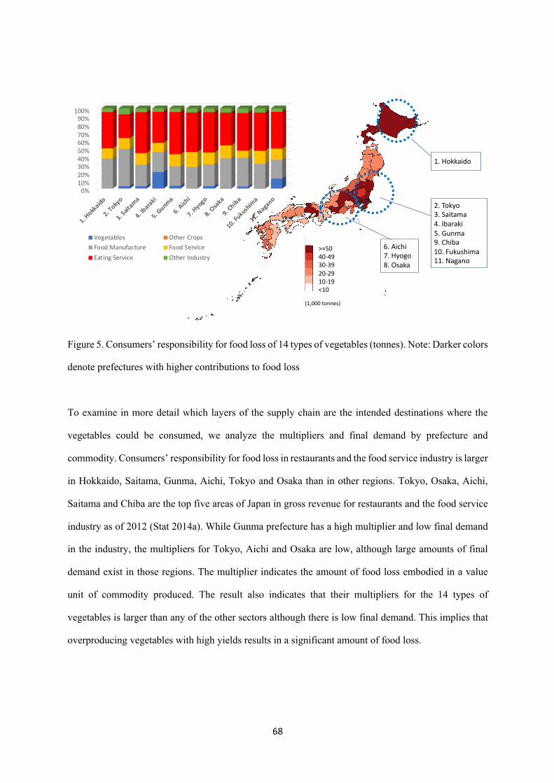
68

Figure 5. Consumers’ responsibility for food loss of 14 types of vegetables (tonnes). Note: Darker colors

denote prefectures with higher contributions to food loss

To examine in more detail which layers of the supply chain are the intended destinations where the

vegetables could be consumed, we analyze the multipliers and final demand by prefecture and

commodity. Consumers’ responsibility for food loss in restaurants and the food service industry is larger

in Hokkaido, Saitama, Gunma, Aichi, Tokyo and Osaka than in other regions. Tokyo, Osaka, Aichi,

Saitama and Chiba are the top five areas of Japan in gross revenue for restaurants and the food service

industry as of 2012 (Stat 2014a). While Gunma prefecture has a high multiplier and low final demand

in the industry, the multipliers for Tokyo, Aichi and Osaka are low, although large amounts of final

demand exist in those regions. The multiplier indicates the amount of food loss embodied in a value

unit of commodity produced. The result also indicates that their multipliers for the 14 types of

vegetables is larger than any of the other sectors although there is low final demand. This implies that

overproducing vegetables with high yields results in a significant amount of food loss.

>=5040-4930-3920-2910-19<10

2. Tokyo3. Saitama4. Ibaraki5. Gunma9. Chiba10. Fukushima11. Nagano

1. Hokkaido

6. Aichi7. Hyogo8. Osaka

0%10%20%30%40%50%60%70%80%90%

100%

1. Hokkaido

2. Tokyo

3. Sait

ama

4. Ibaraki

5. Gunma

6. Aich

i

7. Hyogo

8. Osaka

9. Chiba

10. Fukushim

a

11. Nagano

Vegetables Other Crops

Food Manufacture Food Service

Eating Service Other Industry

(1,000 tonnes)

69

3.3.3. Environmental burdens related to the food loss footprint

As described in this paper, we identify the responsibility of consumers as well as producers for food

losses of 14 types of vegetables. One of the aims of our analysis is to identify the responsibility for food

loss both from a producer perspective and a demand-side perspective, and at the same time, to raise

awareness of consumers role in food loss. Production of vegetables emits GHG, uses energy, and

introduces nitrogen, potassium oxide and phosphorus pentoxide into soil through the use of agricultural

fertilizers. Such pollution is emitted where the vegetables are grown, although the production would be

required for industries and consumers in other regions. The vegetables discarded in fields are also

produced for the benefit of consumers. Figure 6 depicts the GHG emissions from a consumption

perspective. Consequently, the figure indicates the degree to which environmental burdens are borne

by consumers. As one might expect, Hokkaido shoulders a large amount of the burden for GHG

emissions compared to other areas (Figure 6). That is true because a large proportion of those vegetables

are intended to be consumed through production or provision of food-related products in regions with

high population, production of food manufacturing products, and gross revenue in restaurants and the

food service industry. The results also demonstrate that the amounts of nitrogen, potassium oxide, and

phosphorus pentoxide are high in Hokkaido because agricultural crops such as potatoes and carrots

require higher amounts of these fertilizers than other agricultural crops (MAFF 2016). Overall, our

results demonstrate that avoiding food loss and producing only the amounts that consumers’ need would

reduce 2,133,736 tCO2eq of GHG. By reducing food loss, absorption of 6,145 tonnes of nitrogen, 2,301

tonnes of potassium oxide, and 9,185 tonnes of phosphorus pentoxide could be avoided. In our analysis,

we only consider the emissions generated by cultivating 14 types of vegetables, and do not consider

those from other crops. This is because in this paper, we aim to identify the responsibility for the

emissions attributable to the 14 subject vegetables that are discarded in the fields.

70

Figure 6: GHG emissions generated via consumption of 14 subject vegetables discarded in the field

3.4. Discussion

Prevention of food loss is a key issue for sustainability and food security, as it requires efficient

utilization of resources such as land, water, and energy. We analyze production-based food loss for 14

vegetables types in Japan and establish consumers’ responsibility for those food losses using a Japan

MRIO database. Footprint analysis using MRIO data is able to quantify the impact exerted by the entire

supply chain. Through our analysis, we identify where the food that ends up lost is produced, and where

that food’s potential consumers reside. Japanese people have reduced the amount of food they waste by

introducing recycling policies. As the next step, the Japanese government must consider adopting

measures and policies to reduce food loss. Although a discussion of the supply and demand adjustment

for vegetable production was conducted in 2007 (MAFF 2007b), there is no concrete policy or current

action to reduce food loss. In fact, while 17% of the total production of the 14 types of vegetables were

discarded in fields in 2007, only a two percent reduction was achieved for field disposal from 2007 to

2014.

0

100

200

300

400

Hokk

aido

Aom

ori

Iwat

eM

iyag

iAk

itaYa

mag

ata

Fuku

shim

aIb

arak

iTo

chig

iG

unm

aSa

itam

aCh

iba

Toky

oKa

naga

wa

Niig

ata

Toya

ma

Ishi

kaw

aFu

kui

Yam

anas

hiN

agan

oG

ifuSh

izuok

aAi

chi

Mie

Shig

aKy

oto

Osa

kaHy

ogo

Nar

aW

akay

ama

Tott

ori

Shim

ane

Oka

yam

aHi

rosh

ima

Yam

aguc

hiTo

kush

ima

Kaga

wa

Ehim

eKo

chi

Fuku

oka

Saga

Nag

asak

iKu

mam

oto

Oita

Miy

azak

iKa

gosh

ima

Oki

naw

a

GHG

emiss

ions

(10

00 tC

O2e

q)

Prefecture

71

Target setting for achieving the SDG of sustainable production and consumption is one measure toward

reducing food loss. For instance, farmers, food businesses, and consumers together can discuss how to

reduce losses by making use of vegetables that are otherwise disposed of by setting a clear reduction

target. Then, the progress toward achieving the target can be measured by establishing baselines and

methodologies (Australian Government 2017). To establish baselines, a comprehensive picture of the

amount of food loss and the trade flow of agricultural crops are required. Consequently, the first step to

reducing food loss is to identify where and how much food is lost (Buzby and Hyman 2012; Johnson et

al., 2018), and to enhance communication and cooperation between farmers (FAO 2011), buyers, and

consumers throughout the supply chain (Seminar 2016).

Our analysis identifies that a significant amount of vegetables is harvested but not delivered to markets.

Some reasons for this food loss are overproduction, lowering demand, or nonstandard shapes of

vegetables. These issues could be solved by enhancing communication and the transparency of mutual

linkages among producers, industries, and consumers. By revealing the linkages of stakeholders in food

loss, farmers, buyers, consumers, and policymakers can find measures to reduce that loss by region and

by stakeholder. In fact, food waste and loss in medium/high-income countries occurs mainly due to

“consumer behaviour as well as the lack of coordination between different actors in the supply chain”

(FAO, 2011, page v), and because of the difficulty in predicting the numbers of buyers and consumers

(Buzby and Hyman 2012).

In our study, to identify such linkages between production and consumption, we conduct a food loss

footprint analysis. The food loss footprint can reveal intended transactions for agricultural crops that

are presumed to be delivered to the market, but which are discarded in fields without being consumed.

Such transactions extend from Hokkaido at the north end of Japan to Okinawa, Japan’s southernmost

prefecture. One finding from our agricultural food loss footprint analysis is that densely populated

regions such as Tokyo, Osaka and Saitama have more responsibility for agricultural food loss than less-

populated regions, because of their higher demand for those crops. However, less-populated regions

also bear a high burden of consumers’ responsibility for the food loss, because such regions have a high

72

multiplier and/or high demand for vegetables. For instance, if factories making processed foods are

located in a region, then this region bears responsibility for agricultural food loss because it exerts

intermediate demand for the agricultural crops to produce the foods. In this way, tracing a supply chain

of food loss using a footprint analysis helps to elucidate where such loss is generated and where it is

intended to be delivered. Identifying how much and what types of vegetables are discarded in fields

could help farmers plan crop production and distribution, cooperate with other farmers to reduce food

loss, identify potential markets for crops such as nonstandard vegetables, and investigate alternative

destinations of overproduced agricultural crops to markets with a shortage of the crops. Such

information can also help consumers, industry and policymakers to raise awareness of food loss (Buzby

and Hyman 2012).

Mutual communication and coordination involving producers, buyers, and consumers will be more

necessary than ever before whilst climate change intensifies. As described earlier, food loss occurs in

part because of unpredictable weather. Therefore, if climate change comes to pose severe difficulties,

field disposal may have to be implemented more frequently because of increasing uncertainty about

annual and seasonal agricultural production (Lobell et al., 2011; Campbell et al., 2016). That could

occur because “a changing climate engenders changes in the frequency, intensity, spatial extent,

duration and timing of extreme weather and climate events, and can result in unprecedented extreme

weather and climate events” (IPCC, 2012, page 5). It affects annual agricultural production. Moreover,

farmers tend to produce excess quantities of crops beyond the quantity likely to be demanded to cope

with unexpected weather events as well as pest damage (Kodera and Isobe 2016). Therefore, food loss

is expected to become a more important issue to tackle in terms of food security and reducing

environmental burdens, along with achieving the SDG targets.

73

3.5. References

ALIC. 2017. “Act on Stabilization of Production and Shipment of Vegetables (Japanese).”

https://www.alic.go.jp/content/000139232.pdf.

———. 2018. “Supply and Demand Data for Potatoes.” Agriculture & Livestock Industries

Corporation. http://www.alic.go.jp/starch/japan/data/kokunai1-(2)-a.pdf.

Andrew, Robbie, Glen P Peters, and James Lennox. 2009. “APPROXIMATION AND REGIONAL

AGGREGATION IN MULTI-REGIONAL INPUT–OUTPUT ANALYSIS FOR NATIONAL

CARBON FOOTPRINT ACCOUNTING.” Economic Systems Research 21 (3). Routledge:311–

35. https://doi.org/10.1080/09535310903541751.

Australian Government. 2017. “National Food Waste Strategy: Halving Australia’s Food Waste by

2030.” Government Department of the Environment, Australian.

https://www.environment.gov.au/system/files/resources/4683826b-5d9f-4e65-9344-

a900060915b1/files/national-food-waste-strategy.pdf.

Bobbink, R., K. Hicks, J. Galloway, T. Spranger, R. Alkemade, M. Ashmore, M. Bustamante, et al.

2010. “Global Assessment of Nitrogen Deposition Effects on Terrestrial Plant Diversity: A

Synthesis.” Ecological Applications 20 (1). Ecological Society of America:30–59.

https://doi.org/10.1890/08-1140.1.

Booth, Anne. 2012. “Indonesia Rising: The Repositioning of Asia’s Third Giant.” In Indonesia

Update Series: College of Asia and the Pacific, The Australian National University and ISEAS

Singapore, xxiv +198.

Buzby, Jean C., and Jeffrey Hyman. 2012. “Total and per Capita Value of Food Loss in the United

States.” Food Policy 37 (5). Pergamon:561–70.

https://doi.org/10.1016/J.FOODPOL.2012.06.002.

Campbell, Bruce M., Sonja J. Vermeulen, Pramod K. Aggarwal, Caitlin Corner-Dolloff, Evan

Girvetz, Ana Maria Loboguerrero, Julian Ramirez-Villegas, et al. 2016. “Reducing Risks to

Food Security from Climate Change.” Global Food Security 11 (December). Elsevier:34–43.

https://doi.org/10.1016/J.GFS.2016.06.002.

Capone, Roberto, Hamid El Bilali, Philipp Debs, Gianluigi Cardone, and Noureddin Driouech. 2014.

74

“Food System Sustainability and Food Security: Connecting the Dots.” Journal of Food Security

2 (1). Science and Education Publishing:13–22. https://doi.org/10.12691/jfs-2-1-2.

Charlton, Karen E. 2016. “Food Security, Food Systems and Food Sovereignty in the 21st Century: A

New Paradigm Required to Meet Sustainable Development Goals.” Nutrition and Dietetics 73

(1):3–12. http://ro.uow.edu.au/smhpapers/3477.

Clapp, Jennifer. 2017. “Food Self-Sufficiency: Making Sense of It, and When It Makes Sense.” Food

Policy 66 (January). Pergamon:88–96. https://doi.org/10.1016/J.FOODPOL.2016.12.001.

Cu Cek, Lidija, Ji Rí, Jaromír Kleme S, and Zdravko Kravanja. 2012. “A Review of Footprint

Analysis Tools for Monitoring Impacts on Sustainability.” Journal of Cleaner Production 34:9–

20. https://doi.org/10.1016/j.jclepro.2012.02.036.

Dixie, Grahame. 2005. “Horticultural Marketing.” FOOD AND AGRICULTURE ORGANIZATION

OF THE UNITED NATIONS. http://www.fao.org/docrep/008/a0185e/a0185e00.htm#Contents.

Engström, Rebecka, and Annika Carlsson-Kanyama. 2004. “Food Losses in Food Service Institutions

Examples from Sweden.” Food Policy 29 (3). Pergamon:203–13.

https://doi.org/10.1016/J.FOODPOL.2004.03.004.

FAO. 2006. “Policy Brief Changing Policy Concepts of Food Security.”

http://www.foodsecinfoaction.org/.

———. 2008. “CLIMATE CHANGE AND FOOD SECURITY: A FRAMEWORK DOCUMENT

FOOD AND AGRICULTURE ORGANIZATION OF THE UNITED NATIONS ROME,

2008.” http://www.fao.org/forestry/15538-079b31d45081fe9c3dbc6ff34de4807e4.pdf.

———. 2011. “Global Food Losses and Food Waste – Extent, Causes and Prevention.”

http://www.fao.org/docrep/014/mb060e/mb060e00.pdf.

———. 2016. “FOOD AND AGRICULTURE: Key to Achieving the 2030 Agenda for Sustainable

Development 2.” http://www.fao.org/3/a-i5499e.pdf.

Gruber, Nicolas, and James N Galloway. 2008. “An Earth-System Perspective of the Global Nitrogen

Cycle.” Nature 451 (January). Nature Publishing Group:293.

http://dx.doi.org/10.1038/nature06592.

Grunert, Klaus G., Sophie Hieke, and Josephine Wills. 2014. “Sustainability Labels on Food

75

Products: Consumer Motivation, Understanding and Use.” Food Policy 44 (February).

Pergamon:177–89. https://doi.org/10.1016/J.FOODPOL.2013.12.001.

Gustavsson, Jenny, Christel Cederberg, Ulf Sonesson, and Andreas Emanuelsson. 2013. “The

Methodology of the FAO Study: "Global Food Losses and Food Waste-Extent, Causes

and Prevention"-FAO, 2011.” http://www.diva-

portal.org/smash/get/diva2:944159/FULLTEXT01.pdf.

Harris Farm. 2018. “15 Million Kilos of Imperfect Picks Sold.” Harris Farm Markets News, 2018.

Hasegawa, Ryoji, Shigemi Kagawa, Makiko Tsukui, and Hasegawa@oiu Jp. 2011. “Carbon Footprint

Analysis through Constructing a Multi-Region Input–output Table: A Case Study of Japan.”

https://doi.org/10.1186/s40008-015-0015-6.

Hitomi, KAZUMI, and PONGSUN Bunditsakulchai. 2008. “Development of Multi-Regional Input

Output Table for 47 Prefectures in Japan (Japanese).” Central Res. Inst. Electric Power Ind.,

Socio-Economic Res. Center, JPN, no. Y07035.

Hobbs, Jill E., and Linda M. Young. 2000. “Closer Vertical Co‐ordination in Agri‐food Supply

Chains: A Conceptual Framework and Some Preliminary Evidence.” Supply Chain

Management: An International Journal 5 (3):131–43.

https://doi.org/10.1108/13598540010338884.

Hoekstra, Arjen Y, and Thomas O Wiedmann. 2014. “Humanity’s Unsustainable Environmental

Footprint.” Science (New York, N.Y.) 344 (6188). American Association for the Advancement of

Science:1114–17. https://doi.org/10.1126/science.1248365.

Hokkaido Government. 2018. “Agriculture in Hokkaido Japan.” Department of Agriculture, Hokkaido

Government. http://www.pref.hokkaido.lg.jp/ns/nsi/genjyou_english_3001.pdf.

IPCC. 2012. “Summary for Policymakers. In: Managing the Risks of Extreme Events and Disasters to

Advance Climate Change Adaptation.” A Special Report of Working Groups I and II of the

Intergovernmental Panel on Climate Change. Cambridge University Press, Cambridge, UK, and

New York, NY, USA, 1–19. https://www.ipcc.ch/pdf/special-

reports/srex/SREX_FD_SPM_final.pdf.

Irani, Zahir, Amir M. Sharif, Habin Lee, Emel Aktas, Zeynep Topaloğlu, Tamara van’t Wout, and

76

Samsul Huda. 2017. “Managing Food Security through Food Waste and Loss: Small Data to Big

Data.” Computers & Operations Research, November. Pergamon.

https://doi.org/10.1016/J.COR.2017.10.007.

Johnson, Lisa K., Rebecca D. Dunning, J. Dara Bloom, Chris C. Gunter, Michael D. Boyette, and

Nancy G. Creamer. 2018. “Estimating on-Farm Food Loss at the Field Level: A Methodology

and Applied Case Study on a North Carolina Farm.” Resources, Conservation and Recycling

137 (October). Elsevier:243–50. https://doi.org/10.1016/J.RESCONREC.2018.05.017.

Kimura, M. 2013. “Mechanism of Occurrence of Food Loss and Disposal in Japan - A Study on

Suppression of Agricultural Product Disposal -.” Chuo Gakuin University.

http://www2.cgu.ac.jp/kyouin/yamada/link/kyou13/1302kimu.pdf.

Kodera, Masaya, and Seiichiro Isobe. 2016. “Research on Production Waste of Vegetables in Japan.”

Nihon University_, Production Engineering Dept. http://www.cit.nihon-

u.ac.jp/laboratorydata/kenkyu/kouennkai/reference/No.49/pdf/P-95.pdf.

Kronenberg, T. 2009. “Construction of Regional Input-Output Tables Using Non-Survey Methods -

the Role of Cross-Hauling.” International Regional Science Review 32:40–64.

Kummu, M., H. de Moel, M. Porkka, S. Siebert, O. Varis, and P.J. Ward. 2012. “Lost Food, Wasted

Resources: Global Food Supply Chain Losses and Their Impacts on Freshwater, Cropland, and

Fertiliser Use.” Science of The Total Environment 438 (November). Elsevier:477–89.

https://doi.org/10.1016/J.SCITOTENV.2012.08.092.

Kurasaka, H., Ogawa, M., Suzuki, T., Tateda, R., Hashino, T. 2010. “Stable Supply of Vegetables.”

Inter-University Seminar for the Future of Japan. http://www.isfj.net/articles/2010/l05.pdf.

Lenzen, Manfred. 2013. “Unifying Global Approaches to Multi-Regional Input-Output Analysis and

Environmental Footprinting A Project Réunion Project Centre for Integrated Sustainability

Analysis.” University of Sydney.

http://www.isa.org.usyd.edu.au/mrio/Global_MRIO_Réunion.pdf.

Lenzen, Manfred, Arne Geschke, Arunima Malik, Jacob Fry, Joe Lane, Thomas Wiedmann, Steven

Kenway, Khanh Hoang, and Andrew Cadogan-Cowper. 2017. “Economic Systems Research

New Multi-Regional Input–output Databases for Australia – Enabling Timely and Flexible

77

Regional Analysis New Multi-Regional Input–output Databases for Australia – Enabling Timely

and Flexible Regional Analysis.” ECONOMIC SYSTEMS RESEARCH 29 (2):275–95.

https://doi.org/10.1080/09535314.2017.1315331.

Lenzen, Manfred, Arne Geschke, Thomas Wiedmann, Joe Lane, Neal Anderson, Timothy Baynes,

John Boland, et al. 2014. “Compiling and Using Input–output Frameworks through

Collaborative Virtual Laboratories.” https://doi.org/10.1016/j.scitotenv.2014.03.062.

Lenzen, Manfred, Keiichiro Kanemoto, Daniel Moran, and Arne Geschke. 2012. “Mapping the

Structure of the World Economy.” Environmental Science & Technology.

https://doi.org/10.1021/es300171x.

Lenzen, Manfred, Arunima Malik, Steven Kenway, Peter Daniels, Ka Leung Lam, and Arne Geschke.

2018. “Economic Damage and Spill-Overs from a Tropical Cyclone.” Natural Hazards and

Earth System Sciences Discussions, January, 1–28. https://doi.org/10.5194/nhess-2017-440.

Lenzen, Manfred, Daniel Moran, Keiichiro Kanemoto, and Arne Geschke. 2013. “BUILDING

EORA: A GLOBAL MULTI-REGION INPUT–OUTPUT DATABASE AT HIGH COUNTRY

AND SECTOR RESOLUTION.” Economic Systems Research 25 (1). Routledge:20–49.

https://doi.org/10.1080/09535314.2013.769938.

Lenzen, Manfred, Joy Murray, Fabian Sack, and Thomas Wiedmann. 2007. “Shared Producer and

Consumer Responsibility — Theory and Practice.” Ecological Economics 61 (1). Elsevier:27–

42. https://doi.org/10.1016/J.ECOLECON.2006.05.018.

Lenzen, Manfred, Lise-Lotte Pade, and Jesper Munksgaard. 2004. “CO2 Multipliers in Multi-Region

Input-Output Models.” Economic Systems Research 16 (4). Routledge:391–412.

https://doi.org/10.1080/0953531042000304272.

Lenzen, Manfred, Ya-Yen Sun, Futu Faturay, Yuan-Peng Ting, Arne Geschke, and Arunima Malik.

2018. “The Carbon Footprint of Global Tourism.” Nature Climate Change 8 (6):522–28.

https://doi.org/10.1038/s41558-018-0141-x.

Leontief, Wassily. 1970. “Environmental Repercussions and the Economic Structure: An Input-

Output Approach.” The Review of Economics and Statistics 52 (3). The MIT Press:262–71.

http://www.jstor.org/stable/1926294.

78

Lobell, David B, Wolfram Schlenker, and Justin Costa-Roberts. 2011. “Climate Trends and Global

Crop Production Since 1980.” Science 333 (6042):616 LP-620.

http://science.sciencemag.org/content/333/6042/616.abstract.

MAFF. 2007a. “Committee on Emergency Supply and Demand Adjustment Method of Vegetables.”

http://www.maff.go.jp/j/study/other/kinkyu_jukyu/pdf/report.pdf.

———. 2007b. “Committee Report on Emergency Supply and Demand Adjustment Method of

Vegetables (Japanese).” Committee on Emergency Supply and Demand Adjustment Method of

Vegetables. http://www.maff.go.jp/j/seisan/ryutu/yasai_zyukyu/y_zyukyu/sankou/pdf/1-2.pdf.

———. 2007c. “Possibility to Respond to Diverse Needs for Fresh Sales of Agricultural Products and

Processing / Business - Nonstandard Vegetables for Diverse Needs (Japanese).”

http://www.maff.go.jp/j/study/syoku_cost/pdf/data03_5.pdf.

———. 2015a. “Fruit and Vegetables Wholesale Market Research (Japanese).” https://www.e-

stat.go.jp/stat-

search/files?page=1&layout=datalist&toukei=00500226&tstat=000001015623&cycle=7&year=

20140&month=0&tclass1=000001020455&tclass2=000001076367.

———. 2015b. “Fruit and Vegetables Wholesale Market Research by Production (Japanese).”

https://www.e-stat.go.jp/stat-


20140&month=0&tclass1=000001020455&tclass2=000001076367.

———. 2015c. “Survey of Fruits Production (Japanese).” Ministry of Agriculture, Forestry and

Fisheries. http://www.maff.go.jp/j/tokei/kouhyou/sakumotu/sakkyou_kazyu/index.html.

———. 2015d. “Survey of Local Specialty Vegetable Production.” Ministry of Agriculture, Forestry

and Fisheries.

———. 2015e. “Survey of Vegetable Production (Japanese).” Ministry of Agriculture, Forestry and

Fisheries. https://www.e-stat.go.jp/stat-


20140&month=0&tclass1=000001032286&tclass2=000001032933&tclass3=000001077555.

———. 2016. “Prefectural Fertilization Standard (Japanese).” Ministry of Agriculture, Forestry and

79

Fisheries. http://www.maff.go.jp/j/seisan/kankyo/hozen_type/h_sehi_kizyun/index.html.

Mattsson, Kristina. 2014. “Why Do We Throw Away Edible Fruit and Vegetables?”

https://www2.jordbruksverket.se/download/18.37e9ac46144f41921cdb38b/1398671573352/ra14

_5eng.pdf.

Mekonnen, M. M., and A. Y. Hoekstra. 2011. “The Green, Blue and Grey Water Footprint of Crops

and Derived Crop Products.” Hydrology and Earth System Sciences 15 (5):1577–1600.

https://doi.org/10.5194/hess-15-1577-2011.

METI. 2014. “Statistical Charts for Industry (Japanese).” Ministry of Economy, Trade and Industry.

http://www.meti.go.jp/statistics/tyo/kougyo/result-2.html.

MIC. 2015. “2011 Input-Output Tables.” Ministry of Internal Affairs and Communications.

http://www.soumu.go.jp/english/dgpp_ss/data/io/io11.htm.

MOE. 2017. “Usage of Food Waste (FY2014) (Japanese).” Ministry of Enviornment.

https://www.env.go.jp/press/103939.html.

NIES. 2018. “Embodied Energy and Emission Intensity Data for Japan Using Input-Output Tables.”

National Institute for Environmental Studies, Japan.

http://www.cger.nies.go.jp/publications/report/d031/jpn/index_j.htm.

Poore, J, and T Nemecek. 2018. “Reducing Food’s Environmental Impacts through Producers and

Consumers.” Science, 987–92. http://science.sciencemag.org/.

Rockström, Johan, Malin Falkenmark, Louise Karlberg, Holger Hoff, Stefanie Rost, and Dieter

Gerten. 2009. “Future Water Availability for Global Food Production: The Potential of Green

Water for Increasing Resilience to Global Change.” Water Resources Research 45 (7).

https://doi.org/10.1029/2007WR006767.

Seminar, Kudang Boro. 2016. “Food Chain Transparency for Food Loss and Waste Surveillance.”

Journal of Developments in Sustainable Agriculture 11:17–22.

https://www.jstage.jst.go.jp/article/jdsa/11/1/11_17/_pdf.

Stat. 2014a. “Economic Census for Business Activity (Japanese).” Statistics Japan.

http://www.stat.go.jp/data/e-census/2012/kakuho/gaiyo.html.

———. 2014b. “Population (Japanese).” Statistics Japan. https://www.e-stat.go.jp

80

Tamura, Yuka. 2015. “Effective Utilisation of Unutilised Vegetables - Possibility of Vegetable Sheet

Processing - (Japanese).” Journal of Kyoto Seika University 47. http://www.kyoto-

seika.ac.jp/researchlab/wp/wp-content/uploads/no_tamura_yuka.pdf.

Többen, J., and T.H. Kronenberg. 2015. “Construction of Multi-Regional Input-Output Tables Using

the CHARM Method.” Economic Systems Research 27:487–507.

Tsuruta, Hiromi, Keisuke Tusge, Takashi Yoshimura, Teruyoshi Yanagita, and Koji Nagao. 2007.

“Research on Development of Food Materials by Utilising Unused Resources - _impacts of

Using Lotus Root Powder for Lipid Metabolism in Obese / Diabetic Model Mice - (Japanese).”

Industrial Technology Center of SAGA Research Report. https://www.saga-

itc.jp/var/rev0/0003/1205/p51-53.pdf.

UN. 2015. “Transforming Our World: The 2030 Agenda for Sustainable Development.” General

Assembley 70 Session 16301 (October):1–35. https://doi.org/10.1007/s13398-014-0173-7.2.

Wiedmann, Thomas. 2009. “A Review of Recent Multi-Region Input–output Models Used for

Consumption-Based Emission and Resource Accounting.” Ecological Economics 69 (2).

Elsevier:211–22. https://doi.org/10.1016/J.ECOLECON.2009.08.026.

Wiedmann, Thomas, and Manfred Lenzen. 2018. “Environmental and Social Footprints of

International Trade.” Nature Geoscience 11 (5):314–21. https://doi.org/10.1038/s41561-018-

0113-9.

Wu, Decun, and Jinping Liu. 2016. “Multi-Regional Input-Output (MRIO) Study of the Provincial

Ecological Footprints and Domestic Embodied Footprints Traded among China’s 30 Provinces.”

Sustainability 8 (1345).

Zaks, D P M, C C Barford, N Ramankutty, and J A Foley. 2009. “Producer and Consumer

Responsibility for Greenhouse Gas Emissions from Agricultural Production—a Perspective

from the Brazilian Amazon.” Environmental Research Letters 4 (4):44010.

https://doi.org/10.1088/1748-9326/4/4/044010.

Zhang, Chao, and Laura Diaz Anadon. 2014. “A Multi-Regional Input–output Analysis of Domestic

Virtual Water Trade and Provincial Water Footprint in China.” Ecological Economics 100

(April). Elsevier:159–72. https://doi.org/10.1016/J.ECOLECON.2014.02.006.

81

3.6. Appendix

The classifications of the 19 sectors are ‘14 types of vegetables’, ‘other agricultural’, three major food

business stakeholders (‘food manufacturing’, ‘food-related business and the social service industry’,

and ‘restaurant and food service industry’), and ‘other’. The ‘Other agricultural’ sector includes

livestock because potatoes are used as food in industries such as dairy cattle farming and hogs. The

aggregation of the three stakeholders in food-related businesses is listed in Table 1 below. The remining

sectors listed in Japan’s Input Output table 2011 are aggregated into the ‘other’ sector.

Table 1. List of aggregated food business sectors used for our analysis and classification in

the Japan Input Output table 2011. Sectors aggregated for analysis Japan National IO classification (MIC 2015) Food manufacture Meat

Beef Pork Chicken meat Miscellaneous meat

By-products of slaughtering and meat processing

Processed meat products Bottled or canned meat products Dairy farm products Drinking milk

Dairy products

Frozen fish and shellfish Salted, dried or smoked seafood Bottled or canned seafood Fish paste Miscellaneous processed seafood

Grain milling Milled rice Miscellaneous grain milling Flour and miscellaneous grain milled products Wheat flour

Miscellaneous grain milled products

Noodles Bread

Confectionery

82

Bottled or canned vegetables and fruits

Preserved agricultural foodstuffs (except bottled or canned)

Sugar Refined sugar Miscellaneous sugar and by-products of sugar manufacturing Starch Dextrose, syrup and isomerized sugar Animal oil and fats, vegetable oil and meal Vegetable oil Animal oils and fats Cooking oil Vegetable meal

Condiments and seasonings

Prepared frozen foods Retort foods Dishes, sushi and lunch boxes School lunch (public) School lunch (private)

Miscellaneous foods

Refined sake Malt liquors Whiskey and brandy

Miscellaneous liquors

Soft drinks Restaurant and food service industry Eating and drinking services

Food related business and social services

Hotels

Sport facility service, public gardens and amusement parks Ceremonial occasions Medical service (hospitalization) Medical service (dentistry) Medical service (miscellaneous medical service) Social welfare (public) Social welfare (private, non-profit) Social welfare (profit-making) Nursing care (facility services) Nursing care (except facility services) Services relating to air transport Private non-profit institutions serving households, n.e.c.

83

Chapter 4 Assessing carbon footprints of cities

4.1. Introduction

A major part of the global population lives in cities and urban areas, and cities are home to half of the

world’s population (Hiremeth et at 2013, Wigginton et al 2016). As centres of economic and social

activities, as well as engines of growth in the global economy, cities are driving consumption and

associated environmental impacts (Chavez and Sperling 2017; McCormick et al 2013). Urban residents

and activities contribute to about 80% of global greenhouse gas (GHG) emissions (World Bank, 2013),

and China has become the largest GHG emitter globally due to both economic growth and urbanization

(Liu et al., 2012). Metropolitan areas also play a dominant role in sustainable development and climate

change mitigation, because they have the potential to innovate and initiate low-carbon infrastructure

pathways as well as influence changes in lifestyles (Bailey 2017; Creutzig et al. 2016; Dasgupta, 2015;

Dhakal and Ruth 2017; Wheeler and Beatley, 2014). There are several alliances such as the C40 group

of cities or the recently launched Global Covenant of Mayors for Climate & Energy (launched March

2017), that promote sustainability in urban policy and decision making, and provide model case studies.

Cities are by no means autonomous but rely on natural resources from other regions within a country

or from the rest of the world. As a consequence, cities inevitably cause carbon emissions, natural

resource use and are responsible for environmental impacts beyond their geographical boundaries (Bai

2007; Lenzen and Peters 2010). Therefore, in terms of urban carbon mitigation, it is important to

consider the reduction of emissions related to trade.

China ratified the Paris Climate Change Agreement, and has committed to cut carbon emissions by 60-

65% per unit of GDP by 2030 compared with 2005 levels (The Guardian 2016). One objective of the

Chinese 2016-2020 Five-Year Plan for national economic development is that more developed cities

84

should reach the peak of their emissions ahead of the nation (WRI 2016). This is relevant because 80%

of total Chinese national GHG emissions can be attributed to activities in Chinese cities (Liu 2015),

highlighting the important roles that Chinese cities are playing in national carbon mitigation.

As a basis for action on climate change, cities need to quantify and report their greenhouse gas (GHG)

emissions (Dodman 2011; Ibrahim et al. 2012; Kennedy et al. 2012; Ramaswami et al. 2012a; Lin et

al. 2013). There is general agreement that comprehensive urban emission inventories should not only

include the territorial emissions but also those that occur outside of the city boundary but are caused by

activities in the city. Consumption-based accounting at the urban scale (synonymous with carbon

footprint accounting) has been identified as complementary to territorial emissions accounting (Chavez

and Ramaswami 2011; Kennedy and Sgouridis 2011; Baynes and Wiedmann 2012; Ramaswami et al.

2012b; Chavez and Ramaswami 2013a; Feng et al., 2014). Because of its comprehensiveness, input-

output analysis (IOA) has been applied widely to estimate the whole of life cycle carbon emissions of

cities (Chen et al. 2016a; Chen et al. 2016b; Chen et al. 2016c; Wiedmann et al. 2016a). Importantly,

footprint obtained by using methods that do not employ IOA suffer from severe systematic truncation

errors (Lenzen 2000; Lenzen and Dey 2000) that render comparisons and decision-making infeasible

(Lenzen and Treloar 2003).

4.1.1. Input-output approach to footprint

Ever since the IOA has been introduced, it has been applied in studies at city scale (Hirsch 1959; Tiebout

1960; Hirsch 1963), often using national IO tables combined with data for local household expenditure.7

Some cities have their own official IO tables (Morrison and Smith 1974; Smith and Morrison 1974),

and these have been used in studies of input-output modelling for urban economies and carbon

emissions (Chen et al., 2013; Wang et al., 2013; Yao et al., 2013). However, using only single-region

IO data fails to distinguish the range of technologies employed to produce imports. Inter-regional or

7 Heinonen et al., 2013 a; Ala-Mantila et al., 2013; Ala-Mantila et al., 2014; Larsen and Hertwich, 2010a., Larsen and Hertwich,

2009; Larsen and Hertwich, 2010b; Larsen and Hertwich, 2011; Dias et al., 2014, Chen et al. 2016a, Minx et al. 2013, Moll

and Norman 2002; Lenzen et al. 2004a; Baynes et al. 2011; Wiedenhofer et al. 2011; 2013.

85

multi-regional methods are better suited for estimating the spatial interdependence or connectedness of

cities (Miller and Blair, 2009; Gordon and Ledent 1980).

Originally, city-scale consumption-based carbon accounting was based on national-scale IO tables, by

establishing national average carbon intensities for all sectors and multiplying them with local

household expenditure data for matching product groups to obtain consumption-based household

carbon footprints (Larsen and Hertwich 2009; 2010a; b; Ala-Mantila et al. 2013; Chavez and

Ramaswami 2013b; Dias et al. 2014; Heinonen 2017). This has often resulted, however, in carbon

footprints being smaller than the production-based emissions because the carbon footprints in those

studies not taking into account investment by governments and businesses due to a lack of such data at

the city-scale (Chen et al. 2016b, Wiedmann et al. 2016b). In other words, the system boundaries related

to production and consumption-based activities that are normally adopted in IOA at the national scale

were not always applied consistently at the city scale. Furthermore, the inevitable assumption of

national-scale models is that the carbon intensity of local products equals the carbon intensity of

imported products, an assumption that creates a potentially significant error (Lenzen et al. 2004a;

Wiedmann et al. 2016b; Heinonen 2017; Ramaswami et al. 2017).

Some Chinese cities have their own single-region input-output table which are published every 5 years.

They allow using city-scale carbon intensities and complete final demand including expenditure and

investment of governments and businesses (Zhou et al. 2010; Guo et al. 2012; Chen et al. 2013).

However, the Chinese official single-region IO tables have only one column for domestic and overseas

imports and exports, respectively (Mi et al. 2016; Shao et al. 2016). This has hampered the

understanding of the origin and destination of emissions embodied in trade between cities and their

domestic and global hinterlands. In contrast, the provincial multi-region input-output (MRIO) table

constructed by Liu et al. 2012 only covers four provincial cities (Beijing, Shanghai, Tianjin and

Chongqing) and other provinces with a limited number of sectors. It is nevertheless the most used MRIO

table for Chinese carbon footprint accounting studies (Feng et al. 2013; Feng et al. 2014; Liu et al.

2015). The construction of the Rest-of-World (RoW) region for city-scale MRIO tables is regarded a

86

challenge as there is usually no published data that records the trade between a city and the rest of the

world. Most regional import and export estimations adopt non-survey methods (Ivanova and Stelder

2009; Sargento et al. 2012; Többen and Kronenberg 2015).

There was a lack of city-scale MRIO tables for most Chinese cities, until recently Wang et al. 2015b;

Wang 2017 have developed a comprehensive Chinese MRIO table combined with greenhouse gas

satellite accounts, covering 30 Chinese provinces nested into an inter-provincial and international

MRIO structure. This database was estimated by combining downscaled national tables with extensive

survey data, for example trade data provided by Chinese customs agencies, and by embedding into a

tiered inter-regional and international model, combining Chinese data with the Eora global MRIO

database (Lenzen et al. 2013b). This new framework enables comprehensive city-scale carbon footprint

accounting as the import from the Rest of the world (RoW) region makes up a non-negligible part of

the total carbon footprint of cities (Lin et al. 2015; Chen et al. 2016d).

4.1.2. Aim of this study

Given that Wang et al’s MRIO database makes it possible for any Chinese city to use IOA to determine

its carbon footprint in a comprehensive way, the following question can be addressed. What errors occur

when a less complete and detailed databases is used? In order to support decision-making, findings of

quantitative footprint studies should be accompanied by estimates of uncertainty. Without such

uncertainty estimates, comparisons of GHG emission of cities or benchmarking cannot be carried out

reliably. The aim of this study is to explore potential errors and uncertainties associated with city carbon

foot printing by comparing and analysing a number of cases with different levels of information of city

input-output data. In the following we will first illustrate eight representative cases of different levels

of data availability, i.e. different levels of aggregation and completeness. For this purpose, we use four

case studies including Beijing, Shanghai, Chongqing and Tianjin. For each case study, we curtail and

aggregate Wang et al’s comprehensive global MRIO database to simulate different levels of data

availability. We then calculate the carbon footprint of each case by applying Leontief’s demand-pull

approach. Finally, we calculate and compare the deviation of the various city carbon footprint results

87

with Wang et al’s 2015 database which we take as the “true” reference case because of the high level

of disaggregation and completeness of data. Our ultimate goal is to conclusively identify levels of data

availability that do not allow calculation of sufficiently accurate carbon footprints, and thus provide

guidance to decision-makers involved in urban environmental issues.

4.2. Methods and data

In principle, no city is self-sufficient in producing all the goods it needs (Rees and Wackernagel 1996),

and hence virtually every city of the world trades with its national hinterland (Lenzen and Peters 2010)

and with the rest of the world. Cities thus mobilize natural resources and exert environmental pressure

and impact beyond their boundaries (Folke et al. 1997). This means that in order to assess a city’s

carbon or resource footprint, local, national and global data of final demand, for intermediate

transactions, carbon emissions and natural resource use are needed. Such comprehensive data is

however rarely available. A number of options are possible for methodological simplification, that is,

for limiting the assessment scope to match the available data.

4.2.1. Truncation errors associated with non-IO methods

The first simplification is not to use input-output analysis at all, but collecting bottom-up statistics of a

city’s economic activities and the carbon emission attributes thereof. Such an approach is often referred

to as process analysis (PA; Moskowitz and Rowe 1985). The PA approach usually provides an accurate

picture of the footprint of those activities that occur directly in the city under investigation. However,

it usually fails to adequately take into account the footprints of production occurring in the supply-chain

of the city (Bullard et al. 1978). This information gap is due to the labour-intensive nature of the bottom-

up data collection process. At some stage, inputs into the city’s footprint are deemed negligible, and a

narrow system boundary is drawn around the footprint assessment (Suh et al. 2004). This narrow scope

for the system boundary leads to significant systematic truncation errors (Lenzen 2000). Such

truncation errors can be estimated using Leontief standard demand-pull input-output formulation: 𝐹 =

𝐐𝐱=)*(𝐈 − 𝐓𝐱=)*))*𝐲T , where F is the city’s (carbon/resource) footprint, Q is the (carbon/resource)

satellite account accompanying the (MR)IO database, T is the nested global intermediate transactions

matrix, 𝐱 = 𝐓𝟏𝐓+𝐲𝟏𝐲 is total economic output (determined as row-wise sums across intermediate

88

demand T and final demand y, denoted using summation operators 1T and 1y), 𝐲T is the city’s final

demand, I is an identity matrix matching the dimensions of T, and the hat symbol denotes

diagonalisation of a vector. The supply-chain network underpinning a city’s economic activities can be

unravelled by expanding the Leontief inverse 𝐋 = (𝐈 − 𝐓𝐱=)*))* ≡ (𝐈 − 𝐀))* into an infinite series

𝐋 = 𝐈 + 𝐀 + 𝐀= + 𝐀> +⋯ (Waugh 1950). Each power of the coefficients matrix A describes a

production layer. A city’s carbon footprint is then 𝐹 = 𝐐𝐱=)*𝐲T + 𝐐𝐱=)*𝐀𝐲T + 𝐐𝐱=)*𝐀=𝐲T + 𝐐𝐱=)*𝐀>𝐲T +

⋯ , where the term 𝐐𝐱=)*𝐲T represents emissions of the city’s immediate suppliers, 𝐐𝐱=)*𝐀𝐲T are

(indirect) emissions of the city’s suppliers’ suppliers, and so on. Bottom-up process analyses usually do

not venture beyond the first- or second-order production layers, and thus truncate the assessment scope

by omitting higher-order supply chains contributing to the overall footprint. In this work, we quantify

the number of supply-chain stages that need to be enumerated in order to achieve reasonable

completeness of carbon footprints. We demonstrate that such completeness is out of bounds for bottom-

up process analyses.

4.2.2. Effect of data quality on footprint measures

The ideal data situation is for a city input-output table to be accompanied by a) import and export data

detailed by partner country and sector, and b) by city-specific carbon and natural resource use satellite

accounts. In addition, this city input-output table should be embedded in a nested multi-region input-

output (MRIO) structure (Leontief 1953; Leontief and Strout 1963), distinguishing the rest of the

country that the city is located in, and the rest of the world detailed by country and sector (see Bachmann

et al. 2015 and Wenz et al. 2015). A database with such characteristics is available for China, in time

series (Wang et al. 2015a).

The China MRIO database established by Wang et al. (2015) is a hierarchically nested system of

subnational and international MRIO tables for the period 1997 to 2011, distinguishing 30 provincial

regions of China and linking each province with 185 countries. The MRIO tables feature complete

interregional trade and regional-international trade with 135 sectors for each province. Four of the 30

provincial regions, Beijing, Tianjin, Shanghai, and Chongqing, are municipalities directly under the

89

central government, that is, each of them represent a “city” at the provincial level and form part of the

first tier of administrative divisions of China. The rest of the world is represented by 189 countries and

about 10,000 sectors in the Eora MRIO database (Lenzen et al. 2012; Lenzen et al. 2013a), into which

the Chinese provinces are embedded.

Any other available city input-output tables will deviate from the ideal table described above in the

sense that they have one or more of the ideal components missing or aggregated. In the following we

describe an approach by which we successively curtail and aggregate data around a particular city in

Wang et al’s database. In other words, we simulate a number of incomplete and/or aggregated data

situations, in order to obtain an estimate of the likely errors introduced by using city input-output tables

of varying degrees of incompleteness and/or aggregation. For each successive curtailment and

aggregation, we determine that city’s carbon footprint. By using Wang et al’s full database as the

reference point, we are able to calculate the difference between the incomplete/aggregated and the “true”

carbon footprint.

For the regional aggregation to work, inter-provincial and international trade matrices must be

expressed in the same sectoral classification. In a first step, we therefore aggregate the Wang et al’s

nested provincial and global data into a common, 26-sector classification. Following from there, we

examine eight cases (Table. 1).

90

A) Trade partners represented

by Ns = 26 sectors

B) Trade partners represented

by Ns = 1 sector

i) Fully populated nested

MRIO structure with

international and inter-

provincial feedback

Nd = 29 provincial trade

partners,

Ni = 188 international trade

partners


partners,


partners

ii) City IO and MRIO

databases separated, no


provincial feedback


partners,


partners


partners,


partners

iii) City IO and MRIO

databases separated, no


provincial feedback

Nd = 1 provincial trade partner

(remainder of country, “Rem

C”),


partner (rest of world, “RoW”)

Nd = 1 provincial trade partner

(remainder of country, “Rem

C”),


partner (rest of world, “RoW”)

iv) SRIO setting, no outside

regional entity

Domestic transactions and

imports matrices added

Only domestic transactions

matrix

Table 1: Eight cases of curtailing and aggregating trade information from a city input-output table nested

in an inter-provincial and international MRIO table.

These eight cases of curtailing and aggregating trade information from a city input-output table nested

in an inter-provincial and international MRIO table are visualised in Fig. 1. For example, cases ii-iv

match situations where city exports are not provided by using sector, and as such an integration into an

MRIO structure is not possible without making broad assumptions. Cases B apply where the city’s trade

is not detailed by product or sector, and cases iii refer to situations where imports are not known by

trading partner. Case A-iv reflects any situation where a statistical office publishes national input-output

tables with indirect allocation of competing imports. An example for model Biii is discussed by Mi et

al. 2016; Shao et al. 2016.

91

A B RC Ct D E F A B RC Ct D E F

| | | | | || | | | | || | | | | || | | | | || | | | | || | | | | || | | | | || | | | | |

A AB BRC RCCt CtD DE EF F

A B RC Ct D E F A B RC Ct D E F

A AB BRC RC

Ct Ct

D DE EF F

Rem C Ct RoW Rem C Ct RoW

RC RC

Ct Ct

RW RW

Ct+RoW Ct

Ct Ct

case A-iv case B-iv

case A-i case B-i

case A-ii case B-ii

case A-iii case B-iii

Value addedCity in C

City

in

C

Intermediate demand Final demandCity in C

Value addedCity in C

City

in

C +

RoW

Intermediate demand Final demandCity in C + RoW

Rem C City in C RoWValue added

City

in

CRo

WR

em C

Final demandRem C City in C RoW

Value addedCity in C RoW

Intermediate demand

Rem

CCi

ty i

n C

RoW

Final demandCity in C RoW

Rem C

Rem CIntermediate demand

F

Value addedA B Rem C City in C D E F

A

B

Rem

CCi

ty i

n C

D

E

Final demandA B Rem C City in C D E F

Intermediate demand


City

in C

D

E

F

A

B

Rem

C

Intermediate demand Final demandA B Rem C City in C D E F

++

+

++

F+A B Rem C City in C D E

+ + + + +

Value added

+ +

F + + + + + + +

+ + + + + +

+ + + + +

E + + + +

+

City

in

C

D + + + + + + +

+ + + + + +

+ + + +

Rem

C

+ + + + +

+

B + + + + + + + +

+ + + + + +A + + + + +



City

in

C

D

E

F

A

B

Rem

C


92

Figure 1: Visualisation of the data available for the eight cases listed in Tab. 1. Each panel shows a

quadratic intermediate transactions table with the city IO table represented in dark grey, a vertical final

demand block to the right with the city final demand dot-hatched, and a horizontal value-added block

with city value added cross-hatched. Letter A-F denote countries, ‘Ct’ = city in country C, ‘Rem C’ =

“RC” = remainder of country C, ‘RoW’ = ‘RW’ = rest of world. Trade blocks hatched with many

horizontal or vertical lines indicate rest-of-world and rest-of-country data availability by exporting and

importing sector. Trade blocks represented by one line indicate rest-of-world and rest-of-country data

aggregated into one sector. A ‘+’ sign indicates one trade number.

Footprints for these eight cases can be enumerated as follows:

• For cases i, Leontief’s demand-pull formulation (see Section 2.1) applies. Cases Ai and Bi are

different only in the size of the trade blocks (189*26´189*26 versus 189*1´189*1).

• Cases ii and iii can be enumerated by employing Miyazawa’s partitioned inverse (Miyazawa and

Masegi 1963; Miyazawa 1968). Assume a two-region MRIO system

𝐓 = W𝐓%? 𝟎𝐙 𝐓@AB

Z , (1)

where Tct is the city input-output transactions matrix, TRoW is Wang’s MRIO system with China net

of the city, and Z are the RoW-to-city import blocks. As explained earlier, the city’s exports cannot

be integrated because column detail is assumed unavailable. Miyazawa’s calculus then yields

𝐋 = (𝐈 − 𝐓𝐱=)*))* =W 𝐋%? 𝟎𝐋@AB𝐙𝐋%? 𝐋@AB

Z , with

𝐋%? = .𝐈 − 𝐓%?𝐱%?2)*/

)* and 𝐋@AB = .𝐈 − 𝐓@AB𝐱@AB[ )*/

)* , (2)

where 𝐋 = (𝐈 − 𝐓𝐱=)*))* is called the Leontief inverse. Once again, cases Aii, Aiii, Bii and Biii are

different only in the size of the trade blocks Z (Aii: 189*26´189*26; Bii: 189*1´189*1; Aiii:

2*26´2*26; Biii: 2*1´2*1). Footprints can then be evaluated by inserting L as in equation 2 into

Leontief’s demand-pull form.

• Cases iv are evaluated by taking Q, T, x, and y from the single-region IO system, and again

following Leontief’s demand-pull.

93

4.2.3. Comparisons between footprint results

The standard Leontief formula 𝐹 = 𝐐𝐱=)*(𝐈 − 𝐓𝐱=)*))*𝐲T assumes that city final demand 𝐲T is a vector,

and connects factor inputs 𝐐𝐱=)*, the Leontief inverse 𝐋 = (𝐈 − 𝐓𝐱=)*))*, and final demand by matrix

products. Thus, the carbon or resource footprint F becomes a scalar. It is also possible to connect the

three factors by element-wise products, ie 𝐅ℙ = 𝐐𝐱=)*,(𝐈− 𝐓𝐱=)*))*𝐲T or 𝐅𝕊 = 𝐐𝐱=)*(𝐈 − 𝐓𝐱=)*))*𝐲]̂ .

Here, 𝐅ℙ and 𝐅𝕊 are 189*26´1-sized vector representations of the footprint by sets of producing (ℙ)

and selling (𝕊 ) countries and sectors, respectively (Kanemoto et al. 2012). A 189*26´189*26

representation of the footprint by both producing and selling country and sector is 𝐅ℙ𝕊 =

𝐐𝐱=)*,(𝐈− 𝐓𝐱=)*))*𝐲Ta . In Section 3.1 we present simplifications of 𝐅ℙ𝕊 with ℙ = 𝕊 =

{City, RemainderofChina, RestofWorld}.

Taking Wang et al’s full nested MRIO database as the reference point, we are able to calculate the

matrix difference between each of the eight cases and the “true” carbon footprint. Matrix differences

can be chosen from Wiebe and Lenzen 2016 and Abd Rahman et al. 2017, and comparisons between

the cases can be visualised using multidimensional scaling. In this study, we employ the cross-entropy

matrix distance measure.

The errors described in this work are unfortunately not the only shortcomings for city CF analysis.

Often, city IO databases are obtained through non-survey methods that cut out the regional economic

structure from the national IO database and regional employment or output weights. Non-survey

methods have been tested extensively against real-world survey-based data (Bonfiglio and Chelli 2008;

Sargento et al. 2012), and it has become clear that some of these methods introduce quite severe mis-

estimation. These errors are completely independent of the deficiencies described in this work, and add

to the overall uncertainty in carbon footprints. For further insights on non-survey mis-estimations in the

context of city carbon footprints, see Wiedmann et al. 2017.

4.3. Results

4.3.1. Carbon footprints of Beijing, Shanghai, Chongqing and Tianjin

Table 2 contains the footprints for the four cities sliced by final demand origin (the end of supply chains

– the regions that sell the final product to the city) and emissions origin (the beginning of supply chains

– the regions from which the emissions originated). For each city, final demand is cut into three broad

origins: the city, the remainder of country (RemC), and the rest of the world (RoW). These footprints

were calculated using Wang et al’s Chinese MRIO nested within the complete Eora MRIO (186 regions

and approximately 15,000 sectors in total).

94

Emissions origin City RemC RoW Total

Beijing final demand segment

Beijing 2,621 7,092 19,636 29,348 RemC 38 5,441 5,418 10,897 RoW 9 930 134,260 135,200 Total 2,668 13,463 159,310 175,440

Chongqing final demand

segment

Chongqing 3,505 2,075 5,000 10,580 RemC 17 3,347 4,678 8,042 RoW 1 78 5,035 5,115 Total 3,523 5,500 14,713 23,736

Shanghai final demand segment

Shanghai 3,644 5,811 24,882 34,337 RemC 58 10,697 11,264 22,019 RoW 62 884 96,801 97,747 Total 3,764 17,392 132,950 154,100

Tianjin final demand segment

Tianjin 2,397 3,472 7,786 13,654 RemC 66 6,641 5,970 12,676 RoW 14 525 20,538 21,076 Total 2,477 10,637 34,294 47,407

Table 2: City footprints 𝑭ℙ𝕊 by emissions origin (columns) and region of final sale (kilotonnes CO2-

e), with with ℙ = 𝕊 = {𝑪𝒊𝒕𝒚, 𝑹𝒆𝒎𝒂𝒊𝒏𝒅𝒆𝒓𝒐𝒇𝑪𝒉𝒊𝒏𝒂, 𝑹𝒆𝒔𝒕𝒐𝒇𝑾𝒐𝒓𝒍𝒅, 𝑨𝒍𝒍𝒓𝒆𝒈𝒊𝒐𝒏𝒔}.

The total carbon footprints in Table 2 translate into per-capita carbon footprints of 8.1 t/cap (Beijing,

21.5 million inhabitants), 6.4 t/cap (Shanghai, 24.2 million), 7.3 t/cap (Tianjin, 6.4 million), and 5.6

t/cap (Chongqing, 4.3 million). These values are within range of the Chinese average per-capita

emissions of about 7.6 t/cap.

The first three row sums in the four panels in Table 2 show that Beijing and Shanghai import significant

emissions embodied in products demanded from RoW, while Chongqing and Tianjin rely more on

inputs from their city and the rest of China. This is because first, Beijing and Shanghai are

administrative and financial centres where city businesses are concentrated on services provision, and

second because these cities are coastal trade hubs. Hence these cities import “material” and emissions-

intensive products from abroad. In contrast, Chongqing and Tianjin feature more primary and

manufacturing such as of chemical products, electronic equipment, motor vehicles, steel and textiles.

In addition, Tianjin features oil refining and Chongqing food processing. Third, the column sums in

the four panels in Table 2 show that most emissions ultimately originate in the rest of the world,

followed by the rest of China. The cities themselves are of minor importance as emitters, which is

understandable given that on the whole, emissions-intensive primary and secondary industries are likely

located outside of cities.

95

Beijing

Chongqing

Rank Product Footprint (kt) Product Footprint (kt)

1 Construction; RoW 4,589 Construction; Cq 959

2 Construction; RoCh 3,039 Construction; RoW 729

3

Public Management and Social

Organization; RoW 957 Construction; RoCh 719

4 Real Estate; RoW 828 Catering Services; RoW 464

5

Banking, Security, Other Financial

Activities; RoW 818

Production and Supply of Electric Power

and Heat Power; Cq 417

6 Health; RoW 686 Animal Husbandry; RoW 379

7 Manufacture of Electronic Component; RoW 672 Farming; RoW 294

8 Education; RoW 668 Transport Via Road; Cq 135

9

Research and Experimental Development;

RoW 590


Organization; RoW 131

10 Construction; Bj 548 Farming; Cq 124

11 Manufacture of Computer; RoW 500 Real Estate; RoW 122

12 Catering Services; RoW 497


Activities; RoW 121

13

Telecom & Other; information Transmission

Services; RoW 470 Grinding of Grains; RoW 118

14

Manufacture of Communication Equipment;

RoW 368 Hotels; RoW 115

15

Production and Supply of Electric Power and

Heat Power; RoCh 345 Education; RoW 102

16


Organization; RoCh 341 Health; RoW 99

17


Activities; RoCh 331 Refining of Vegetable Oil ; RoW 97

18

Processing of Petroleum and Nuclear Fuel;

RoW 327 Animal Husbandry; Cq 96

19 Manufacture of Automobiles; RoW 313 Catering Services; Cq 89

20


Heat Power; Bj 308


Organization; Cq 89

96

Table 3: Carbon footprint (kt CO2-e) of top-ranking 20 products sold in each city, together with their

emissions origin, based on the reference MRIO database. For example, “Real Estate; RoW” means a)

the carbon footprint of real estate businesses in the city rendering services to city residents and the

government, and b) the carbon footprint of those parts of these real estate businesses’ supply chains that

originate in the rest of the world. Full product details are given in Appendix 1.1.

Shanghai

Tianjin

Rank Product Footprint Product Footprint

1 Construction; RoW 5,419 Construction; RoW 2,018

2 Construction; RoCh 2,761 Construction; RoCh 1,827

3 Catering Services; RoW 1,157 Construction; Tj 766

4 Construction; Sh 1,138


and Heat Power; Tj 570

5 Animal Husbandry; RoW 1,037 Manufacture of Electronic Component; RoW 367

6 Grinding of Grains; RoW 861 Manufacture of Computer; RoW 353

7 Refining of Vegetable Oil ; RoW 693 Catering Services; RoW 340

8




RoW 294

9 Processing of Forage; RoW 606 Grinding of Grains; RoW 284

10 Real Estate; RoW 568 Wholesale and Retail Trades; RoW 282

11


Activities; RoW 554

Manufacture of Household Audiovisual

Apparatus ; RoW 238

12 Manufacture of Electronic Component; RoW 546 Refining of Vegetable Oil ; RoW 235

13 Health; RoW 509 Processing of Forage; RoW 173

14 Education; RoW 487 Animal Husbandry; RoW 167

15 Entertainment; RoW 429 Wholesale and Retail Trades; Tj 163

16 Farming; RoW 417



17 Manufacture of Metal Products; RoW 379 Processing of Other Foods; RoW 147

18 Manufacture of Automobiles; RoW 375 Manufacture of Other Foods; RoW 145

19


Services; RoW 371 Slaughtering and Processing of Meat; RoW 136

20 Hotels; RoW 328 Production and Supply of Electric Power and Heat Power; RoCh 120

97

Beijing

Chongqing

Rank Product Footprint (kt) Product Footprint (kt)

1 Construction; RoW 4,589 Construction; Cq 959

2 Construction; RoCh 3,039 Construction; RoW 729

3


Organization; RoW 957 Construction; RoCh 719

4 Real Estate; RoW 828 Catering Services; RoW 464

5


Activities; RoW 818


and Heat Power; Cq 417

6 Health; RoW 686 Animal Husbandry; RoW 379

7 Manufacture of Electronic Component; RoW 672 Farming; RoW 294

8 Education; RoW 668 Transport Via Road; Cq 135

9

Research and Experimental Development;

RoW 590



10 Construction; Bj 548 Farming; Cq 124

11 Manufacture of Computer; RoW 500 Real Estate; RoW 122

12 Catering Services; RoW 497


Activities; RoW 121

13


Services; RoW 470 Grinding of Grains; RoW 118

14


RoW 368 Hotels; RoW 115

15


Heat Power; RoCh 345 Education; RoW 102

16


Organization; RoCh 341 Health; RoW 99

17


Activities; RoCh 331 Refining of Vegetable Oil ; RoW 97

18

Processing of Petroleum and Nuclear Fuel;

RoW 327 Animal Husbandry; Cq 96

19 Manufacture of Automobiles; RoW 313 Catering Services; Cq 89

20


Heat Power; Bj 308


Organization; Cq 89

98

Table 3 adds detail to Table 2 by listing the top-ranking 20 products sold in each city, together with

their emissions origin. It can be seen that the top footprint in each city is from purchasing construction

services, most likely this is as a result of both breakneck construction activities as well as the high

embodied carbon in construction materials such as cement and steel. As national finance hubs, Beijing

and Shanghai have relatively high-ranking emissions for professional services such as real estate and

banking, and relatively low-ranking emissions from power production. Because of its relative

geographical remoteness and sprawl, Chongqing features top-ranking road transport emissions.

Shanghai and Tianjin have a high proportion of top-ranking footprints related to manufacturing, for

example computers and electronic components.

Shanghai

Tianjin

Rank Product Footprint Product Footprint

1 Construction; RoW 5,419 Construction; RoW 2,018

2 Construction; RoCh 2,761 Construction; RoCh 1,827

3 Catering Services; RoW 1,157 Construction; Tj 766

4 Construction; Sh 1,138


and Heat Power; Tj 570

5 Animal Husbandry; RoW 1,037 Manufacture of Electronic Component; RoW 367

6 Grinding of Grains; RoW 861 Manufacture of Computer; RoW 353

7 Refining of Vegetable Oil ; RoW 693 Catering Services; RoW 340

8




RoW 294

9 Processing of Forage; RoW 606 Grinding of Grains; RoW 284

10 Real Estate; RoW 568 Wholesale and Retail Trades; RoW 282

11


Activities; RoW 554

Manufacture of Household Audiovisual

Apparatus ; RoW 238

12 Manufacture of Electronic Component; RoW 546 Refining of Vegetable Oil ; RoW 235

13 Health; RoW 509 Processing of Forage; RoW 173

14 Education; RoW 487 Animal Husbandry; RoW 167

15 Entertainment; RoW 429 Wholesale and Retail Trades; Tj 163

16 Farming; RoW 417



17 Manufacture of Metal Products; RoW 379 Processing of Other Foods; RoW 147

18 Manufacture of Automobiles; RoW 375 Manufacture of Other Foods; RoW 145

19


Services; RoW 371 Slaughtering and Processing of Meat; RoW 136

20 Hotels; RoW 328 Production and Supply of Electric Power and Heat Power; RoCh 120

99

4.3.2. Truncation errors

Our production layer decomposition (Section 2.1) shows that roughly 50% of a city’s carbon footprint

is caused by the city’s immediate suppliers (layer 1). Including successive upstream production layers

increases the carbon footprint by counting emissions caused by more and more distant supply-chain

actors. The decomposition converges to the totals listed in Table 2.

Figure 2: Cumulative production layer decomposition of the carbon footprints of Beijing (top left),

Chongqing (top right), Shanghai (bottom left) and Tianjin (bottom right) into upstream supply-chain

stages (see Section 2.1). Reasonable completeness (~90%) of the carbon footprints is achieved only

after taking into account all five successive production stages.

It is instructive to work out the number of individual supply chains contained in each layer. Wang et

al’s MRIO database distinguishes more than 15,000 country-sector pairs trading with the Chinese cities.

This means that there are about 15,000 points of emissions by the city’s immediate suppliers. In the

MRIO database, each of the city’s suppliers has 15,000 suppliers themselves. There are therefore

(15,000)2 ≈ 225 million 2nd-order supply chains, and more than 3 trillion 3rd-order supply chains! The

convergence of the decomposition shows that at least five layers are required to achieve roughly 90%

completeness, but even enumerating the second layer is virtually impossible using bottom-up process-

100

type methods. This means that in order to yield reasonably complete, comparable (carbon) footprints,

an assessment must include an input-output calculus for capturing higher-order supply-chain

contributions (Suh and Nakamura 2007).

4.3.3. Effect of deficiencies in the city IO database

We calculated carbon footprints for each of the deficiency cases (cases of missing or aggregated data)

described in Section 4.2.2. Figure 3 shows the carbon footprint for Shanghai, a) split by emissions origin,

for each final demand segment and deficiency case, and the reference case.

None of the aggregated and curtailed case studies adequately matches the reference case, especially

with regard to the cities’ imports from the rest of the world (third column in the column triplets). This

is because the reference database has China’s provinces nested in a full global MRIO structure with

individual world countries represented at a detail of up to 500 sectors. Each of the deficiency cases

distinguishes no more than 26 sectors for the RoW region.

Cases A-ii and B-ii yield very similar results to cases A-i and B-i, respectively. This is because the only

component missing are the exports of the cities, which is evident from the Miyazawa partitioned inverse

in equation 1. In carbon footprint terms, this omission neglects emissions that occur in the city, become

embodied in exports from the city, and are then imported back into the city via more or less circuitous

trade routes involving possibly Chinese provinces and the rest of the world. Such footprint components

are called interregional feedbacks.8

Emissions from products imported from RoW are regionally aggregated for all B-x cases and, compared

to the corresponding A-x case, show that sectoral aggregation carried a larger penalty than regional

aggregation. Cases A-iv and B-iv are particularly severe. Case A-iv includes emissions embodied in

products imported from the rest of China into the city category, which is therefore larger than in other

cases. The IO database for case B-iv misses all trade outside the city boundaries and thus records only

final demand from the city industries and their emissions.

8 There is a large body of literature of such interregional feedback effects in input-output analysis – see Miller 1966; 1969; Gillen and Guccione 1980; Douglas and MacMillan 1983; Miller 1985; 1986; Guccione et al. 1988; Round 1988; Gillen et al. 1991; Round 1991; 2001.

101

Figure 3: Emissions by emissions origin (colours within columns), final demand segment (columns

within each triplet), and deficiency case (groups of column triplets) for Shanghai (kilotonnes CO2-e).

Deviations of carbon footprints from the reference cases can be visualised using multidimensional

scaling techniques. Here, we first used a detailed breakdown (as in Appendix 1.1) of emissions for all

deficiency cases, and calculates pair-wise cross-entropy matrix distances (Abd Rahman et al. 2017).

We then visualised these distances using multi-dimensional scaling (MDS; Section 4.2.3). For each city,

cases A-iv and B-iv are consistently the furthest distance from the reference case, these being the cases

with the highest aggregation and levels of missing data.

0

10,000

20,000

30,000

40,000

50,000

60,000

70,000

80,000

90,000

100,000

City

Rem

C

RoW

City

Rem

C

RoW

City

Rem

C

RoW

City

Rem

C

RoW

City

Rem

C

RoW

City

Rem

C

RoW

City

Rem

C

RoW

City

Rem

C

RoW

City

Rem

C

RoW

Reference A-i A-ii A-iii A-iv B-i B-ii B-iii B-iv

Emission

s(kilotonn

esCO2-e)byorigin

Deficiencycases byfinaldemandsegment

City RemC RoW

102

(a) Beijing

(b) Chongqing

(c) Shanghai

(d) Tianjin

Figure 4: Multidimensional scaling plots for each city, mapping the cross-entropy distances between

the carbon footprints for each deficiency case and the reference case. Distances CEij between the

commodity footprint matrices as in Appendix 1.1 were calculated using the cross-entropy method by

Abd Rahman et al. 2017. Here we plot sgn(CEij) log10(|1000 ´ CEij |).

Averaging all four multidimensional scaling plots (Fig. 5) provides a clear basis for conclusive

observations of the effect of data quality on city carbon footprints:

Ref

A-iA-ii

A-iii

A-iv

B-i

B-ii

B-iiiB-iv

-4

-3

-2

-1

0

1

2

3

4

-4 -2 0 2 4

Ref

A-i

A-ii

A-iii

A-iv

B-i

B-iiB-iii

B-iv

-4

-3

-2

-1

0

1

2

3

4

-4 -2 0 2 4

Ref

A-i

A-ii

A-iii

A-iv

B-i

B-ii

B-iii

B-iv

-4

-3

-2

-1

0

1

2

3

4

-4 -2 0 2 4

Ref

A-i A-ii

A-iii

A-iv

B-i

B-ii B-iii

B-iv

-4

-3

-2

-1

0

1

2

3

4

-4 -2 0 2 4

103

- Methods A-i-iii and B-i-iii form two clusters, thus showing the similarity of sub-versions of the

general regional aggregation (A) and sectoral aggregation (B) approaches. Sectoral aggregation

leads to a worse outcome than regional aggregation in terms of matching the true reference.

- Within the regional aggregation cluster, method A-i (aggregation from maximum sector detail

– as in the Eora MRIO database –to 26 sectors but retaining the full interregional trade structure)

performs best.

- Methods A-ii and B-ii perform only slightly worse than methods A-i and B-i. This means that

interregional feedbacks do not play a large role for city carbon footprints.

- Aggregating imports into the city table (A-iv), or even omitting them (B-iv) leads to

unacceptable results.

Figure 5: Multidimensional scaling plot for all four cities.

Ref

A-i

A-ii

A-iii

A-iv

B-i

B-iiB-iii

B-iv

-3

-2

-1

0

1

2

3

4

0 2 4

104

4.4. Conclusions

In this study, we calculated carbon footprints for four Chinese cities: Beijing, Chongqing, Shanghai

and Tianjin employing a sub-national MRIO for China nested within the global Eora MRIO, we tested

a variety of missing data cases against a reference case. We find that:

- The Miyazawa partitioned inverse is a convenient method that can be used to calculate the footprint

of a city without the need to embed the city’s IO database into an MRIO, just coupling is needed.

- Ignoring city exports to the rest of the country and the world has only a small effect on the city’s

carbon footprint, because the city’s economic feedback onto itself is usually quite weak (Lenzen et

al. 2004b, Moran et al. 2017).

- Data aggregation constitutes a problem for city foot-printing. Especially a high aggregation of

sectors can lead to unacceptable errors.

- Obviously, missing data (e.g. imports, case Biv) rule out any use of the respective table for

comparative city carbon footprint analysis.

- Using IOA, it is easy to distinguish the contribution to the footprint of the city’s residents

(households), its municipal government, and capital expenditure on infrastructure, since IO

databases explicitly define these final demand destinations separately. This aspect is part of ongoing

work of the authors’ teams.

It can be assumed that similar conclusions are valid when assessing indicators other than GHG emission

footprints, such as for example material footprints, water footprints, or energy footprints.

We have systematically assessed variations due to aggregation and truncation in an input-output

approach to urban carbon footprints. The different outcomes reveal the extent to which a practitioner

compromises an assessment when less data is available or more estimations are required to obtain the

city carbon footprint. With this perspective, urban GHG reports may be produced with greater

awareness of these limits and the worth of collecting direct data.

In the context of the Paris Climate agreement, attribution of GHG emissions will continue to be an

important objective and cities will have a major impact in that regard. For setting greenhouse abatement

targets for city, both direct and indirect emissions, i.e. footprints will be of importance. The lack of data

and frameworks that embed city I-O tables in national and regional tables, as we show in this research

is an important obstacle to evidence based policy making. It would be worthwhile for countries to invest

in national I-O frameworks that explicitly represent the economic structure and the final demand of

cities and their relationship to domestic and international trade. Only if such multi-layered I-O

105

frameworks become more readily available a true representation of a cities whole of supply chain

impacts can be demonstrated and well-targeted policy can be developed.

106

4.5. References

Abd Rahman, M.D., B. Los, A. Owen and M. Lenzen (2017) Multi-level comparisons of input–output

tables using Cross-Entropy indicators.

Ala-Mantila, S., J. Heinonen and S. Junnila (2013) Greenhouse Gas Implications of Urban Sprawl in

the Helsinki Metropolitan Area. sustainability 5.

Bachmann, C., M.J. Roorda and C. Kennedy (2015) Developing a multi-scale multi-region input-

output model. Economic Systems Research 27, 172-193.

Bai, X. (2007) Industrial Ecology and the Global Impacts of Cities. Journal of Industrial Ecology 11,

1-6.

Bailey, R. (2017) Potential Transformation Pathways Towards Low-Carbon Cities. In: S. Dhakal and

M. Ruth (eds.) Creating Low Carbon Cities. Cham, Springer International Publishing, 169-

186.

Baynes, T., M. Lenzen, J.K. Steinberger and X. Bai (2011) Comparison of household consumption

and regional production approaches to assess urban energy use and implications for policy.

Energy Policy 39, 7298–7309.

Baynes, T.M. and T. Wiedmann (2012) General approaches for assessing urban environmental

sustainability. Current Opinion in Environmental Sustainability 4, 458-464.

Bonfiglio, A. and F. Chelli (2008) Assessing the behaviour of non-survey methods for constructing

regional input–output tables through a Monte Carlo simulation. Economic Systems Research

20, 243-258.

Bullard, C.W., P.S. Penner and D.A. Pilati (1978) Net energy analysis - handbook for combining

process and input-output analysis. Resources and Energy 1, 267-313.

Chavez, A. and A. Ramaswami (2011) Progress toward low carbon cities: approaches for

transboundary GHG emissions’ footprinting. Carbon Management 2, 471-482.

Chavez, A. and A. Ramaswami (2013a) Articulating a trans-boundary infrastructure supply chain

greenhouse gas emission footprint for cities: Mathematical relationships and policy relevance.

Energy Policy 54, 376-384.

Chavez, A. and A. Ramaswami (2013b) Articulating a trans-boundary infrastructure supply chain

greenhouse gas emission footprint for cities: Mathematical relationships and policy relevance.

Energy Policy.

Chavez, A. and J. Sperling (2017) Key Drivers and Trends of Urban Greenhouse Gas Emissions. In:

S. Dhakal and M. Ruth (eds.) Creating Low Carbon Cities. Cham, Springer International

Publishing, 157-168.

Chen, G., M. Hadjikakou and T. Wiedmann (2016a) Urban carbon transformations: unravelling

spatial and inter-sectoral linkages for key city industries based on multi-region input-output

analysis. Journal of Cleaner Production.

107

Chen, G., T. Wiedmann, M. Hadjikakou and H. Rowley (2016b) City Carbon Footprint Networks.

Energies 9, 602.

Chen, G., T. Wiedmann, Y. Wang and M. Hadjikakou (2016c) Transnational city carbon footprint

networks – Exploring carbon links between Australian and Chinese cities. Applied Energy

184, 1082-1092.

Chen, G., T. Wiedmann, Y. Wang and M. Hadjikakou (2016d) Transnational city carbon footprint

networks–Exploring carbon links between Australian and Chinese cities. Applied Energy.

Chen, G.Q., S. Guo, L. Shao, J.S. Li and Z.-M. Chen (2013) Three-scale input–output modeling for

urban economy: Carbon emission by Beijing 2007. Communications in Nonlinear Science

and Numerical Simulation 18, 2493-2506.

Creutzig, F., P. Agoston, J.C. Minx, J.G. Canadell, R.M. Andrew, C.L. Quere, G.P. Peters, A. Sharifi,

Y. Yamagata and S. Dhakal (2016) Urban infrastructure choices structure climate solutions.

Nature Climate Change 6, 1054-1056.

Dhakal, S. and M. Ruth (2017) Challenges and Opportunities for Transition to Low Carbon Cities. In:

S. Dhakal and M. Ruth (eds.) Creating Low Carbon Cities. Cham, Springer International

Publishing, 1-4.

Dias, A.C., D. Lemos, X. Gabarrell and L. Arroja (2014) Environmentally extended input–output

analysis on a city scale – application to Aveiro (Portugal). Journal of Cleaner Production 75,

118-129.

Dodman, D. (2011) Forces driving urban greenhouse gas emissions. Current Opinion in

Environmental Sustainability 3, 121-125.

Douglas, G.W. and J.A. MacMillan (1983) Significance of interregional feedbacks for Canadian and

regional energy policy decisions. Canadian Journal of Regional Science 6, 251-258.

Feng, K., S.J. Davis, L. Sun, X. Li, D. Guan, W. Liu, Z. Liu and K. Hubacek (2013) Outsourcing CO2

within China. Proceedings of the National Academy of Sciences 110, 11654-11659.

Feng, K., K. Hubacek, L. Sun and Z. Liu (2014) Consumption-based CO 2 accounting of China's

megacities: The case of Beijing, Tianjin, Shanghai and Chongqing. Ecological Indicators 47,

26-31.

Folke, C., Å. Jansson, J. Larsson and R. Costanza (1997) Ecosystem appropriation by cities. Ambio

26, 167-172.

Gillen, W.J. and A. Guccione (1980) Interregional feedbacks in input-output models: some formal

results. Journal of Regional Science 20, 477-482.

Gillen, W.J., A. Guccione and R.E. Miller (1991) Multipliers and feedback effects in interregional

input-output models: a comment. Ricerche Economiche XLV, 121-126.

Gordon, P. and J. Ledent (1980) Modeling the dynamics of a system of metropolitan areas: a

demoeconomic approach. Environment and Planning A 12, 125-133.

108

Guccione, A., W.J. Gillen, P.D. Blair and R.E. Miller (1988) Interregional feedbacks in input-output

models: the least upper bound. Journal of Regional Science 28, 397-404.

Guo, S., L. Shao, H. Chen, Z. Li, J.B. Liu, F.X. Xu, J.S. Li, M.Y. Han, J. Meng, Z.-M. Chen and S.C.

Li (2012) Inventory and input–output analysis of CO2 emissions by fossil fuel consumption

in Beijing 2007. Ecological Informatics 12, 93-100.

Heinonen, J. (2017) A Consumption-Based Hybrid Life Cycle Assessment of Carbon Footprints in

California: High Footprints in Small Urban Households. World Academy of Science,

Engineering and Technology, International Journal of Environmental, Chemical, Ecological,

Geological and Geophysical Engineering 10, 916-923.

Hirsch, W.Z. (1959) Interindustry relations of a metropolitan area. Review of Economics and Statistics

41, 360-369.

Hirsch, W.Z. (1963) Application of input-output techniques to urban areas. In: T. Barna (ed.)

Structural Interdependence and Economic Development. London, UK, MacMillan & Co Ltd,

151-168.

Ibrahim, N., L. Sugar, D. Hoornweg and C. Kennedy (2012) Greenhouse gas emissions from cities:

comparison of international inventory frameworks. Local Environment 17, 223-241.

Kanemoto, K., M. Lenzen, G.P. Peters, D. Moran and A. Geschke (2012) Frameworks for comparing

emissions associated with production, consumption and International trade. Environmental

Science & Technology 46, 172–179.

Kennedy, C., S. Demoullin and E. Mohareb (2012) Cities reducing their greenhouse gas emissions.

Energy Policy 49, 774-777.

Kennedy, S. and S. Sgouridis (2011) Rigorous classification and carbon accounting principles for low

and Zero Carbon Cities. Energy Policy 39, 5259-5268.

Larsen, H.N. and E.G. Hertwich (2009) The case for consumption-based accounting of greenhouse

gas emissions to promote local climate action. Environmental Science & Policy 12, 791-798.

Larsen, H.N. and E.G. Hertwich (2010a) Identifying important characteristics of municipal carbon

footprints. Ecological Economics 70, 60-66.

Larsen, H.N. and E.G. Hertwich (2010b) Implementing Carbon-Footprint-Based Calculation Tools in

Municipal Greenhouse Gas Inventories. Journal of Industrial Ecology 14, 965-977.

Lenzen, M. (2000) Errors in conventional and input-output-based life-cycle inventories. Journal of

Industrial Ecology 4, 127-148.

Lenzen, M., C. Dey and B. Foran (2004a) Energy requirements of Sydney households. Ecological

Economics 49, 375-399.

Lenzen, M. and C.J. Dey (2000) Truncation error in embodied energy analyses of basic iron and steel

products. Energy 25, 577-585.

109

Lenzen, M., K. Kanemoto, D. Moran and A. Geschke (2012) Mapping the structure of the world

economy. Environmental Science & Technology 46, 8374–8381,

http://dx.doi.org/10.1021/es300171x.

Lenzen, M., D. Moran, K. Kanemoto and A. Geschke (2013a) Building Eora: A global multi-region

input-output database at high country and sector resolution. Economic Systems Research 25,

20-49.

Lenzen, M., D. Moran, K. Kanemoto and A. Geschke (2013b) Building Eora: a global multi-region

input–output database at high country and sector resolution. Economic Systems Research 25,

20-49.

Lenzen, M., L.-L. Pade and J. Munksgaard (2004b) CO2 multipliers in multi-region input-output

models. Economic Systems Research 16, 391-412.

Lenzen, M. and G. Peters (2010) How city dwellers affect their resource hinterland – a spatial impact

study of Australian households. Journal of Industrial Ecology 14, 73-90.

Lenzen, M. and G. Treloar (2003) Differential convergence of life-cycle inventories towards upstream

production layers. Journal of Industrial Ecology 6, 137-160.

Leontief, W. (1953) Interregional theory. In: W. Leontief, H.B. Chenery, P.G. Clark, J.S.

Duesenberry, A.R. Ferguson, A.P. Grosse, R.N. Grosse, M. Holzman, W. Isard and H. Kistin

(eds.) Studies in the Structure of the American Economy. New York, NY, USA, Oxford

University Press, 93-115.

Leontief, W.W. and A.A. Strout (1963) Multiregional input-output analysis. In: T. Barna (ed.)

Structural Interdependence and Economic Development. London, UK, Macmillan, 119-149.

Lin, J., Y. Hu, S. Cui, J. Kang and A. Ramaswami (2015) Tracking urban carbon footprints from

production and consumption perspectives. Environmental Research Letters 10, 054001.

Lin, T., Y. Yu, X. Bai, L. Feng and J. Wang (2013) Greenhouse Gas Emissions Accounting of Urban

Residential Consumption: A Household Survey Based Approach. PLoS ONE 8, e55642.

Liu, W., J. Chen, Z. Tang, H. Liu, D. Han and F. Li (2012) Theories and practice of constructing

China’s interregional Input-Output tables between 30 provinces in 2007, China Statistics

Press, Beijing.

Liu, Z. (2015) China’s Carbon Emissions Report 2015. Harvard Kennedy School: Cambridge, UK.

Liu, Z., K. Feng, K. Hubacek, S. Liang, L.D. Anadon, C. Zhang and D. Guan (2015) Four system

boundaries for carbon accounts. Ecological Modelling 318, 118-125.

Mi, Z., Y. Zhang, D. Guan, Y. Shan, Z. Liu, R. Cong, X.-C. Yuan and Y.-M. Wei (2016)

Consumption-based emission accounting for Chinese cities. Applied Energy.

Miller, R.E. (1966) Interregional feedbacks in input-output models: some preliminary results. Papers

of the Regional Science Association 17, 105-125.

Miller, R.E. (1969) Interregional feedbacks in input-output models: some experimental results.

Western Economic Journal 7, 57-70.

110

Miller, R.E. (1985) Upper bounds on the sizes of interregional feedbacks in multiregional input-

output models. Journal of Regional Science 26, 285-306.

Miller, R.E. (1986) Significance of interregional feedbacks for Canadian and regional energy policy

decisions: a comment. Canadian Journal of Regional Science 9, ?

Minx, J.C., G. Baiocchi, T. Wiedmann, J. Barrett, F. Creutzig, K. Feng, M. Förster, P.-P. Pichler, H.

Weisz and K. Hubacek (2013) Carbon footprints of cities and other human settlements in the

UK. Environmental Research Letters 8, 035039.

Miyazawa, K. (1968) Input-output analysis and interrelational income multiplier as a matrix.

Hitotsubashi Journal of Economics 18, 39-58.

Miyazawa, K. and S. Masegi (1963) Interindustry analysis and the structure of income-distribution.

Metroeconomica XV, 89-103.

Moll, H.C. and K.J. Norman (2002) Towards sustainable development at city level: evaluating and

changing the household metabolism in five European cities. Laxenburg, Austria, International

Institute for Applied Systems Analysis (IIASA), National Institute for Advanced Industrial

Science and Technology (AIST), and Sustainable Consumption and Production Unit of the

United Nations Environment Programme (UNEP).

Moran, D., R. Wood and J. Rodrigues (2017) A note on the magnitude of the feedback effect in

environmentally extended multi-region input-output tables. Journal of Industrial Ecology, in

press.

Morrison, W.I. and P. Smith (1974) Nonsurvey input-output techniques at the small area level: an

evaluation. Journal of Regional Science 14, 1-14.

Moskowitz, P.D. and M.D. Rowe (1985) A comparison of input-output and process analysis. In: P.F.

Ricci and M.D. Rowe (eds.) Health and Environmental Risk Assessment. New York, NY,

USA, Pergamon Press, 281-293.

Ramaswami, A., M. Bernard, A. Chavez, T. Hillman, M. Whitaker, G. Thomas and M. Marshall

(2012a) Quantifying Carbon Mitigation Wedges in U.S. Cities: Near-Term Strategy Analysis

and Critical Review. Environmental Science & Technology 46, 3629-3642.

Ramaswami, A., A. Chavez and M. Chertow (2012b) Carbon Footprinting of Cities and Implications

for Analysis of Urban Material and Energy Flows. Journal of Industrial Ecology 16, 783-785.

Ramaswami, A., D. Jiang, K. Tong and J. Zhao (2017) Impact of the Economic Structure of Cities on

Urban Scaling Factors: Implications for Urban Material and Energy Flows in China. Journal

of Industrial Ecology.

Rees, W. and M. Wackernagel (1996) Urban ecological footprints: Why cities cannot be

sustainable—And why they are a key to sustainability. Environmental Impact Assessment

Review 16, 223-248.

Round, J.I. (1988) Multipliers and feedback effects in interregional input-output models. Ricerche

Economiche XLII, 311-324.

111

Round, J.I. (1991) Multipliers and feedback effects in interregional input-output models: a reply.

Ricerche Economiche XLV, 127-130.

Round, J.I. (2001) Feedback effects in interregional input-output models: what have we learned? In:

M.L. Lahr and E. Dietzenbacher (eds.) Input-Output Analysis: Frontiers and Extensions.

London, UK, Macmillan, ?

Sargento, A.L.M., P.N. Ramos and G.J.D. Hewings (2012) Inter-regional trade flow estimation

through non-survey models: an empirical assessment. Economic Systems Research 24, 173-

193.

Shao, L., D. Guan, N. Zhang, Y. Shan and G. Chen (2016) Carbon emissions from fossil fuel

consumption of Beijing in 2012. Environmental Research Letters 11, 114028.

Smith, P. and W.I. Morrison (1974) Simulating the urban economy. London, UK, Pion Limited.

Suh, S., M. Lenzen, G.J. Treloar, H. Hondo, A. Horvath, G. Huppes, O. Jolliet, U. Klann, W. Krewitt,

Y. Moriguchi, J. Munksgaard and G. Norris (2004) System boundary selection in Life-Cycle

Inventories. Environmental Science & Technology 38, 657-664.

Suh, S. and S. Nakamura (2007) Five years in the area of input-output and Hybrid LCA. International

Journal of Life Cycle Assessment 12, 351-352.

theguardian (2016) China ratifies Paris climate change agreement ahead of G20. China ratifies Paris

climate change agreement ahead of G20.

Tiebout, C.M. (1960) Regional and interregional input-output models: an appraisal. In: R.W. Pfouts

(ed.) The techniques of urban economic analysis. West Trenton, NJ, USA, Chandler-Davis

Publishing Co., 395-407.

Többen, J. and T.H. Kronenberg (2015) Construction of multi-regional input-output tables using the

CHARM method. Economic Systems Research 27, 487-507.

Wang, Y. (2017) An industrial ecology virtual framework for policy making in China. Economic

Systems Research, 1-23.

Wang, Y., A. Geschke and M. Lenzen (2015a) Constructing a time series of nested multiregion input–

output tables. International Regional Science Review 38, 1-24.

Wang, Y., A. Geschke and M. Lenzen (2015b) Constructing a Time Series of Nested Multiregion

Input–Output Tables. International Regional Science Review, 0160017615603596.

Waugh, F.V. (1950) Inversion of the Leontief matrix by power series. Econometrica 18, 142-154.

Wenz, L., S.N. Willner, A. Radebach, R. Bierkandt, J.C. Steckel and A. Levermann (2015) Regional

and sectoral disaggregation of multi-regional input-output tables - a flexible algorithm.

Economic Systems Research 27, 194-212.

Wiebe, K.S. and M. Lenzen (2016) To RAS or not to RAS? What is the difference in outcomes in

multi-regional input–output models? Economic Systems Research 28, 383-402.

112

Wiedenhofer, D., M. Lenzen and J.K. Steinberger (2011) Spatial and socioeconomic drivers of direct

and indirect household energy consumption in Australia. In: P. Newton (ed.) Urban

Consumption. Collingwood, Victoria, Australi, CSIRO Publishing, 251-266.

Wiedenhofer, D., M. Lenzen and J.K. Steinberger (2013) Energy requirements of consumption: Urban

form, climatic and socio-economic factors. Energy Policy 63, 696-707.

Wiedmann, T., M. Lenzen, A. Owen, G. Chen, J. Többen, Y. Wang, F. Faturay and H. Wilting (2017)

Expanding a global MRIO for city footprint analysis. 25th International Input-Output

Conference of the International Input-Output Association (IIOA). Atlantic City, USA.

Wiedmann, T.O., G. Chen and J. Barrett (2016a) The Concept of City Carbon Maps: A Case Study of

Melbourne, Australia. Journal of Industrial Ecology 20, 676-691.

Wiedmann, T.O., G. Chen and J. Barrett (2016b) The Concept of City Carbon Maps: A Case Study of

Melbourne, Australia. Journal of Industrial Ecology.

WRI (2016) 5 Questions: What Does China’s New Five-Year Plan Mean for Climate Action? 5

Questions: What Does China’s New Five-Year Plan Mean for Climate Action?

Zhou, S.Y., H. Chen and S.C. Li (2010) Resources use and greenhouse gas emissions in urban

economy: Ecological input–output modeling for Beijing 2002. Communications in Nonlinear

Science and Numerical Simulation 15, 3201-3231.

113

4.6. Appendix

Table 4: City footprints by commodity and emission origin: Commodity footprints for Beijing

Commodity Emission in city

Emission in RoCh

Emission in RoW

Total emissions

Farming 15.47 18.26 218.19 251.92 Forestry 1.00 1.10 15.12 17.22 Animal Husbandry 10.39 13.18 237.41 260.98 Fishery 2.72 3.15 36.02 41.89 Services in Support of Agriculture 0.94 1.04 13.79 15.77 Mining and Washing of Coal 10.18 30.64 119.63 160.45 Extraction of Petroleum and Natural Gas 0.44 0.86 6.97 8.27 Mining of Ferrous Metal Ores 1.08 0.62 11.32 13.01 Mining of Non-Ferrous Metal Ores 0.17 0.29 6.29 6.74 Mining and Processing of Nonmetal Ores and Other Ores 0.44 0.20 2.81 3.45 Grinding of Grains 1.39 5.34 248.09 254.82 Processing of Forage 1.47 4.77 149.76 155.99 Refining of Vegetable Oil 1.56 5.44 201.65 208.66 Manufacture of Sugar 0.13 0.33 16.48 16.94 Slaughtering and Processing of Meat 1.72 5.31 111.88 118.91 Processing of Aquatic Product 0.77 2.03 19.98 22.78 Processing of Other Foods 1.32 4.06 111.07 116.45 Manufacture of Convenience Food 0.54 0.91 41.88 43.33 Manufacture of Liquid Milk and Dairy Products 0.81 1.33 54.57 56.71 Manufacture of Flavoring and Ferment Products 0.50 0.83 39.61 40.94 Manufacture of Other Foods 2.53 4.01 110.06 116.60 Manufacture of Alcohol and Wine 3.21 2.86 73.10 79.17 Processing of Soft Drinks and Purified Tea 2.80 2.31 34.37 39.47 Manufacture of Tobacco 1.11 3.85 45.07 50.02 Spinning and Weaving, Printing and Dyeing of Cotton and Chemical Fiber 0.37 0.66 4.86 5.88 Spinning and Weaving, Dyeing and Finishing of Wool 0.02 0.03 0.41 0.47 Spinning and Weaving of Hemp and Tiffany 0.05 0.08 1.14 1.26 Manufacture of Textile Products 0.03 0.04 0.26 0.33 Manufacture of Knitted Fabric and Its Products 0.08 0.12 0.61 0.81 Manufacture of Textile Wearing Apparel, Footwear and Caps 2.91 8.94 29.61 41.46 Manufacture of Leather, Fur, Feather(Down) and Its Products 1.02 5.87 25.30 32.19 Processing of Timbers, Manufacture of Wood, Bamboo, Rattan, Palm and Straw Products 0.92 2.96 21.88 25.77 Manufacture of Furniture 1.35 2.86 17.93 22.14 Manufacture of Paper and Paper Products 7.82 21.02 125.81 154.65 Printing, Reproduction of Recording Media 5.21 8.41 36.38 50.00 Manufacture of Articles for Culture, Education and Sports Activities 2.01 6.05 27.08 35.14 Processing of Petroleum and Nuclear Fuel 14.17 17.57 326.51 358.25 Coking 1.81 2.60 12.67 17.08 Manufacture of Basic Chemical Raw Materials 2.22 3.64 31.02 36.89 Manufacture of Fertilizers 0.82 1.37 15.97 18.16 Manufacture of Pesticides 0.17 0.27 4.01 4.45 Manufacture of Paints, Printing Inks, Pigments and Similar Products 0.70 1.12 12.82 14.64 Manufacture of Synthetic Materials 2.04 3.34 34.73 40.10 Manufacture of Special Chemical Products 1.59 2.52 27.60 31.71 Manufacture of Chemical Products for Daily Use 0.44 0.72 6.97 8.13 Manufacture of Medicines 1.59 2.84 31.53 35.97 Manufacture of Chemical Fiber 0.55 1.69 23.59 25.83 Manufacture of Rubber 0.71 1.63 12.80 15.14 Manufacture of Plastic 2.00 4.88 59.11 65.98 Manufacture of Cement, Lime and Plaster 15.49 13.80 28.82 58.11 Manufacture of Products of Cement and Plaster 7.97 7.27 18.30 33.55 Manufacture of Brick, Stone and Other Building Materials 12.72 11.57 24.68 48.97 Manufacture of Glass and Its Products 8.49 7.58 21.88 37.96 Manufacture of Pottery and Porcelain 2.74 2.53 9.12 14.39 Manufacture of Fire-resistant Materials 3.48 3.26 9.83 16.57 Manufacture of Graphite and Other Nonmetallic Mineral Products 3.05 2.78 10.31 16.14 Iron-smelting 19.89 9.50 45.87 75.26 Steelmaking 56.60 27.76 106.11 190.46 Rolling of Steel 181.34 87.46 266.97 535.78 Smelting of Ferroalloy 7.12 3.69 15.70 26.51 Smelting of Non-Ferrous Metals and Manufacture of Alloys 14.21 43.04 131.66 188.90 Rolling of Non-Ferrous Metals 12.06 37.24 144.06 193.37

114

Manufacture of Metal Products 16.07 58.27 196.72 271.06 Manufacture of Boiler and Prime Mover 1.70 6.71 17.87 26.28 Manufacture of Metalworking Machinery 1.56 6.17 15.92 23.65 Manufacture of Lifters 1.50 5.94 27.15 34.59 Manufacture of Pump, Valve and Similar Machinery 2.52 10.04 37.21 49.77 Manufacture of Other General Purpose Machinery 9.16 35.97 83.93 129.07 Manufacture of Special Purpose Machinery for Mining, Metallurgy and Construction 3.55 11.05 39.66 54.26 Manufacture of Special Purpose Machinery for Chemical Industry, Processing of Timber and Nonmetals 1.67 5.10 25.18 31.95 Manufacture of Special Purpose Machinery for Agriculture, Forestry, Animal Husbandry and Fishery 0.92 2.80 9.60 13.31 Manufacture of Other Special Purpose Machinery 4.19 13.06 43.84 61.09 Manufacture of Railroad Transport Equipment 0.43 1.94 11.25 13.62 Manufacture of Automobiles 24.97 114.18 313.14 452.29 Manufacture of Boats and Ships and Floating Devices 1.03 4.74 21.74 27.51 Manufacture of Other Transport Equipment 1.54 6.92 31.52 39.97 Manufacture of Generators 1.32 5.72 39.09 46.13 Manufacture of Equipment for Power Transmission and Distribution and Control 2.47 11.33 104.88 118.67 Manufacture of Wire, Cable, Optical Cable and Electrical Appliances 2.99 13.75 116.75 133.50 Manufacture of Household Electric and Non-electric Appliances 2.93 13.53 68.26 84.72 Manufacture of Other Electrical Machinery and Equipment 1.58 7.28 78.69 87.55 Manufacture of Communication Equipment 15.37 71.27 368.05 454.70 Manufacture of Radar and Broadcasting Equipment 4.44 19.45 115.31 139.20 Manufacture of Computer 29.14 128.25 499.80 657.19 Manufacture of Electronic Component 31.24 134.33 672.28 837.85 Manufacture of Household Audiovisual Apparatus 8.11 39.87 244.85 292.82 Manufacture of Other Electronic Equipment 2.77 12.24 85.32 100.33 Manufacture of Measuring Instruments 3.34 9.73 53.55 66.62 Manufacture of Machinery for Cultural Activity & Office Work 2.10 6.50 40.63 49.24 Manufacture of Artwork, Other Manufacture 1.38 2.82 11.19 15.39 Scrap and Waste 0.65 2.36 5.59 8.60 Production and Supply of Electric Power and Heat Power 307.79 344.71 109.06 761.56 Production and Distribution of Gas 0.32 0.34 1.55 2.21 Production and Distribution of Water 0.17 0.37 1.36 1.90 Construction 548.35 3,038.56 4,589.34 8,176.24 Transport Via Railway 15.02 8.72 36.91 60.64 Transport Via Road 24.80 13.78 58.30 96.87 Urban Public Traffic 9.97 5.82 30.57 46.36 Water Transport 20.78 11.49 74.38 106.65 Air Transport 9.12 5.31 24.20 38.63 Transport Via Pipeline 1.30 0.81 6.17 8.28 Loading, Unloading, Portage and Other Transport Services 15.84 8.77 58.91 83.52 Storage 3.84 2.59 57.69 64.12 Post 7.95 8.45 215.30 231.70 Telecom & Other Information Transmission Services 62.23 149.83 470.15 682.21 Computer Services 5.11 13.01 57.34 75.46 Software Industry 7.17 18.75 76.25 102.16 Wholesale and Retail Trades 26.98 33.22 103.10 163.29 Hotels 5.15 11.99 79.52 96.65 Catering Services 39.52 83.29 496.71 619.52 Banking, Security, Other Financial Activities 144.90 330.78 818.36 1,294.04 Insurance 24.41 61.34 237.25 323.00 Real Estate 132.91 304.46 828.44 1,265.80 Leasing 0.21 0.66 4.09 4.95 Business Services 11.54 30.40 124.34 166.28 Tourism 8.94 22.93 103.25 135.11 Research and Experimental Development 57.14 197.67 590.27 845.09 Professional Technical Services 21.91 53.34 155.55 230.80 Services of Science and Technology Exchanges and Promotion 3.69 9.43 44.67 57.79 Geological Prospecting 1.76 4.45 35.20 41.41 Management of Water Conservancy 1.79 4.55 18.96 25.30 Environment Management 2.75 7.15 48.27 58.17 Management of Public Facilities 5.51 14.20 71.80 91.51 Services to Households 36.12 86.83 217.87 340.82 Other Services 33.71 81.26 205.01 319.98 Education 122.86 282.28 667.77 1,072.91 Health 94.08 219.25 686.02 999.34 Social Security 0.81 2.00 12.22 15.04 Social Welfare 0.69 1.68 11.15 13.53 Journalism and Publishing Activities 4.03 10.56 57.84 72.43

115

Broadcasting, Movies, Televisions and Audiovisual Activities 4.99 13.02 65.51 83.52 Cultural and Art Activities 2.52 6.65 44.46 53.63 Sports Activities 0.51 1.20 7.60 9.30 Entertainment 4.88 12.39 48.33 65.60 Public Management and Social Organization 147.46 340.65 956.60 1,444.71

Table 5: City footprints by commodity and emission origin: Footprints for Chongqin (kilotonnes)


Emission in RoCh

Emission in RoW

Total emissions

Farming 124.01 26.83 293.96 444.80 Forestry 10.78 2.35 21.86 34.99 Animal Husbandry 95.67 21.41 379.25 496.32 Fishery 28.07 5.93 61.02 95.01 Services in Support of Agriculture 10.54 2.31 24.11 36.96 Mining and Washing of Coal 81.64 6.71 4.72 93.08 Extraction of Petroleum and Natural Gas 0.57 0.22 1.21 2.00 Mining of Ferrous Metal Ores 5.51 1.00 2.70 9.20 Mining of Non-Ferrous Metal Ores 1.04 0.51 2.02 3.58 Mining and Processing of Nonmetal Ores and Other Ores 1.45 0.30 0.63 2.38 Grinding of Grains 5.46 4.46 117.61 127.53 Processing of Forage 5.89 4.46 77.38 87.73 Refining of Vegetable Oil 5.95 4.65 97.17 107.76 Manufacture of Sugar 1.04 0.71 19.13 20.87 Slaughtering and Processing of Meat 6.34 4.49 45.93 56.75 Processing of Aquatic Product 2.92 1.98 13.07 17.97 Processing of Other Foods 4.69 3.57 58.33 66.59 Manufacture of Convenience Food 1.77 1.24 39.51 42.52 Manufacture of Liquid Milk and Dairy Products 2.37 1.61 43.73 47.71 Manufacture of Flavoring and Ferment Products 1.66 1.17 38.63 41.46 Manufacture of Other Foods 5.68 3.56 58.49 67.73 Manufacture of Alcohol and Wine 6.47 3.07 44.36 53.90 Processing of Soft Drinks and Purified Tea 5.99 2.72 25.47 34.17 Manufacture of Tobacco 6.10 3.90 31.29 41.29 Spinning and Weaving, Printing and Dyeing of Cotton and Chemical Fiber 28.39 9.87 45.05 83.31 Spinning and Weaving, Dyeing and Finishing of Wool 3.30 1.19 6.39 10.88 Spinning and Weaving of Hemp and Tiffany 6.14 2.21 15.64 23.99 Manufacture of Textile Products 2.47 1.27 5.00 8.74 Manufacture of Knitted Fabric and Its Products 6.70 3.53 12.75 22.98 Manufacture of Textile Wearing Apparel, Footwear and Caps 2.13 2.62 7.27 12.01 Manufacture of Leather, Fur, Feather(Down) and Its Products 1.41 1.71 5.33 8.45 Processing of Timbers, Manufacture of Wood, Bamboo, Rattan, Palm and Straw Products 5.70 4.29 14.53 24.53 Manufacture of Furniture 2.26 1.85 6.10 10.22 Manufacture of Paper and Paper Products 3.13 1.73 5.30 10.16 Printing, Reproduction of Recording Media 1.34 1.14 2.79 5.27 Manufacture of Articles for Culture, Education and Sports Activities 0.85 0.73 1.86 3.44 Processing of Petroleum and Nuclear Fuel 1.25 0.48 1.59 3.32 Coking 0.10 0.05 0.17 0.32 Manufacture of Basic Chemical Raw Materials 2.91 0.80 1.55 5.26 Manufacture of Fertilizers 1.78 0.47 1.08 3.33 Manufacture of Pesticides 0.63 0.17 0.65 1.46 Manufacture of Paints, Printing Inks, Pigments and Similar Products 2.75 0.71 1.91 5.38 Manufacture of Synthetic Materials 8.12 2.03 4.44 14.60 Manufacture of Special Chemical Products 5.55 1.41 3.30 10.26 Manufacture of Chemical Products for Daily Use 2.07 0.54 1.46 4.08 Manufacture of Medicines 2.67 1.24 4.03 7.94 Manufacture of Chemical Fiber 1.96 1.45 4.17 7.58 Manufacture of Rubber 1.13 0.71 1.52 3.36 Manufacture of Plastic 3.23 2.33 5.38 10.94 Manufacture of Cement, Lime and Plaster 2.66 0.59 0.60 3.85 Manufacture of Products of Cement and Plaster 1.78 0.40 0.46 2.64 Manufacture of Brick, Stone and Other Building Materials 2.30 0.51 0.53 3.34 Manufacture of Glass and Its Products 1.36 0.31 0.37 2.04 Manufacture of Pottery and Porcelain 0.68 0.16 0.24 1.09 Manufacture of Fire-resistant Materials 1.26 0.29 0.40 1.94 Manufacture of Graphite and Other Nonmetallic Mineral Products 1.18 0.27 0.41 1.85 Iron-smelting 4.69 2.26 3.47 10.42 Steelmaking 14.11 6.54 7.90 28.54 Rolling of Steel 52.05 23.29 21.37 96.71

116

Smelting of Ferroalloy 1.98 0.98 1.90 4.87 Smelting of Non-Ferrous Metals and Manufacture of Alloys 14.46 9.49 10.92 34.87 Rolling of Non-Ferrous Metals 14.23 9.34 10.25 33.82 Manufacture of Metal Products 16.86 15.85 23.52 56.23 Manufacture of Boiler and Prime Mover 13.58 13.43 19.00 46.00 Manufacture of Metalworking Machinery 17.11 16.85 24.27 58.23 Manufacture of Lifters 13.50 13.56 25.26 52.32 Manufacture of Pump, Valve and Similar Machinery 20.86 20.79 32.08 73.73 Manufacture of Other General Purpose Machinery 48.36 47.38 52.53 148.27 Manufacture of Special Purpose Machinery for Mining, Metallurgy and Construction 22.95 23.46 34.39 80.80 Manufacture of Special Purpose Machinery for Chemical Industry, Processing of Timber and Nonmetals 12.23 12.58 24.23 49.05 Manufacture of Special Purpose Machinery for Agriculture, Forestry, Animal Husbandry and Fishery 8.00 8.02 14.58 30.60 Manufacture of Other Special Purpose Machinery 26.32 26.84 37.42 90.57 Manufacture of Railroad Transport Equipment 1.70 2.96 4.21 8.87 Manufacture of Automobiles 28.98 45.11 47.57 121.67 Manufacture of Boats and Ships and Floating Devices 4.47 7.44 9.20 21.11 Manufacture of Other Transport Equipment 5.23 8.57 10.51 24.31 Manufacture of Generators 11.85 12.95 15.33 40.13 Manufacture of Equipment for Power Transmission and Distribution and Control 23.50 26.27 28.31 78.08 Manufacture of Wire, Cable, Optical Cable and Electrical Appliances 27.82 31.13 32.16 91.11 Manufacture of Household Electric and Non-electric Appliances 27.59 30.74 30.95 89.28 Manufacture of Other Electrical Machinery and Equipment 17.60 19.61 23.21 60.42 Manufacture of Communication Equipment 0.09 0.12 0.84 1.05 Manufacture of Radar and Broadcasting Equipment 0.04 0.03 0.31 0.37 Manufacture of Computer 0.24 0.33 1.55 2.11 Manufacture of Electronic Component 0.41 0.56 2.74 3.71 Manufacture of Household Audiovisual Apparatus 0.05 0.05 0.52 0.62 Manufacture of Other Electronic Equipment 0.03 0.02 0.27 0.33 Manufacture of Measuring Instruments 3.12 3.22 6.62 12.96 Manufacture of Machinery for Cultural Activity & Office Work 1.69 1.76 4.82 8.27 Manufacture of Artwork, Other Manufacture 5.27 4.57 10.54 20.39 Scrap and Waste 4.38 3.80 8.05 16.24 Production and Supply of Electric Power and Heat Power 416.79 55.78 25.51 498.07 Production and Distribution of Gas 2.15 2.22 3.71 8.07 Production and Distribution of Water 2.26 2.32 3.70 8.28 Construction 959.36 718.85 728.96 2,407.17 Transport Via Railway 50.13 15.39 32.68 98.20 Transport Via Road 134.81 40.45 79.63 254.88 Urban Public Traffic 20.88 6.59 16.24 43.70 Water Transport 83.20 25.20 58.81 167.20 Air Transport 27.78 8.84 20.36 56.98 Transport Via Pipeline 4.72 1.58 7.28 13.59 Loading, Unloading, Portage and Other Transport Services 47.76 14.65 36.12 98.53 Storage 9.45 3.24 31.47 44.16 Post 16.25 3.00 51.61 70.85 Telecom & Other Information Transmission Services 41.03 31.01 70.32 142.36 Computer Services 5.49 3.61 15.02 24.12 Software Industry 7.62 5.27 20.41 33.30 Wholesale and Retail Trades 21.26 14.91 26.47 62.64 Hotels 20.82 19.69 115.27 155.79 Catering Services 89.05 86.33 464.48 639.86 Banking, Security, Other Financial Activities 87.22 65.04 120.71 272.97 Insurance 19.30 14.50 42.45 76.24 Real Estate 82.75 62.48 121.66 266.89 Leasing 0.36 0.28 2.13 2.77 Business Services 11.42 14.47 34.27 60.17 Tourism 8.92 6.32 23.10 38.34 Research and Experimental Development 2.41 2.19 7.77 12.36 Professional Technical Services 17.66 12.81 32.31 62.78 Services of Science and Technology Exchanges and Promotion 4.63 2.95 14.36 21.93 Geological Prospecting 2.71 1.66 11.36 15.73 Management of Water Conservancy 2.65 1.52 9.49 13.66 Environment Management 3.62 2.26 14.02 19.90 Management of Public Facilities 6.10 4.11 18.37 28.58 Services to Households 26.14 19.20 42.58 87.91 Other Services 24.74 18.12 40.81 83.66 Education 74.26 55.32 101.96 231.55 Health 60.51 45.47 99.03 205.02

117

Social Security 1.35 0.66 6.35 8.36 Social Welfare 1.18 0.56 5.78 7.51 Journalism and Publishing Activities 4.93 3.20 16.08 24.22 Broadcasting, Movies, Televisions and Audiovisual Activities 5.80 3.85 17.52 27.16 Cultural and Art Activities 3.44 2.10 13.25 18.80 Sports Activities 0.99 0.46 4.99 6.44 Entertainment 5.60 3.69 15.73 25.02 Public Management and Social Organization 88.89 66.67 131.28 286.84

Table 6: City footprints by commodity and emission origin: Shanghai footprints (kilotonnes)


Emission in RoCh

Emission in RoW

Total emissions

Farming 21.73 25.60 416.72 464.06 Forestry 1.73 1.71 44.65 48.09 Animal Husbandry 28.31 33.83 1,037.37 1,099.51 Fishery 4.88 5.10 104.29 114.26 Services in Support of Agriculture 1.86 1.87 52.38 56.11 Mining and Washing of Coal 0.00 0.00 0.00 0.00 Extraction of Petroleum and Natural Gas 0.48 0.62 9.85 10.96 Mining of Ferrous Metal Ores 0.00 0.00 0.00 0.00 Mining of Non-Ferrous Metal Ores 0.00 0.00 0.00 0.00 Mining and Processing of Nonmetal Ores and Other Ores 0.00 0.00 0.00 0.00 Grinding of Grains 4.12 16.46 860.85 881.43 Processing of Forage 4.92 16.89 606.39 628.20 Refining of Vegetable Oil 4.44 16.23 692.99 713.66 Manufacture of Sugar 0.61 1.85 108.23 110.69 Slaughtering and Processing of Meat 3.05 10.03 213.88 226.96 Processing of Aquatic Product 0.62 2.00 28.32 30.94 Processing of Other Foods 2.90 9.76 320.08 332.74 Manufacture of Convenience Food 1.26 2.78 144.83 148.87 Manufacture of Liquid Milk and Dairy Products 1.77 3.86 181.71 187.34 Manufacture of Flavoring and Ferment Products 1.17 2.58 137.30 141.04 Manufacture of Other Foods 4.66 9.72 320.00 334.39 Manufacture of Alcohol and Wine 4.36 9.61 301.18 315.15 Processing of Soft Drinks and Purified Tea 4.06 8.12 168.60 180.78 Manufacture of Tobacco 3.53 13.10 222.47 239.10 Spinning and Weaving, Printing and Dyeing of Cotton and Chemical Fiber 1.27 2.33 46.49 50.08 Spinning and Weaving, Dyeing and Finishing of Wool 0.14 0.25 4.43 4.82 Spinning and Weaving of Hemp and Tiffany 0.38 0.72 25.51 26.60 Manufacture of Textile Products 0.08 0.23 2.49 2.80 Manufacture of Knitted Fabric and Its Products 0.22 0.62 6.49 7.33 Manufacture of Textile Wearing Apparel, Footwear and Caps 4.46 11.30 84.14 99.90 Manufacture of Leather, Fur, Feather(Down) and Its Products 2.35 6.31 50.35 59.01 Processing of Timbers, Manufacture of Wood, Bamboo, Rattan, Palm and Straw Products 0.00 0.01 0.04 0.05 Manufacture of Furniture 0.00 0.00 0.01 0.01 Manufacture of Paper and Paper Products 2.24 4.59 34.47 41.30 Printing, Reproduction of Recording Media 0.57 1.77 9.70 12.04 Manufacture of Articles for Culture, Education and Sports Activities 0.10 0.28 1.58 1.96 Processing of Petroleum and Nuclear Fuel 85.32 32.32 279.37 397.02 Coking 10.90 4.98 23.08 38.96 Manufacture of Basic Chemical Raw Materials 9.19 10.10 67.43 86.71 Manufacture of Fertilizers 9.00 9.20 68.05 86.26 Manufacture of Pesticides 1.82 1.89 22.26 25.97 Manufacture of Paints, Printing Inks, Pigments and Similar Products 6.99 6.99 67.03 81.01 Manufacture of Synthetic Materials 25.60 25.47 220.09 271.16 Manufacture of Special Chemical Products 13.16 13.36 117.46 143.97 Manufacture of Chemical Products for Daily Use 4.75 4.91 42.53 52.19 Manufacture of Medicines 7.57 12.63 135.89 156.10 Manufacture of Chemical Fiber 9.74 15.99 172.96 198.69 Manufacture of Rubber 6.16 8.47 58.16 72.79 Manufacture of Plastic 13.42 22.81 207.13 243.36 Manufacture of Cement, Lime and Plaster 0.55 0.75 2.25 3.56 Manufacture of Products of Cement and Plaster 0.28 0.38 1.53 2.19 Manufacture of Brick, Stone and Other Building Materials 0.42 0.59 1.84 2.86 Manufacture of Glass and Its Products 0.20 0.28 1.25 1.73 Manufacture of Pottery and Porcelain 0.02 0.03 0.20 0.26 Manufacture of Fire-resistant Materials 0.18 0.24 1.30 1.72 Manufacture of Graphite and Other Nonmetallic Mineral Products 0.14 0.19 1.23 1.56

118

Iron-smelting 1.75 0.96 5.67 8.38 Steelmaking 10.05 5.23 24.09 39.37 Rolling of Steel 104.96 46.64 160.63 312.22 Smelting of Ferroalloy 0.79 0.46 2.77 4.02 Smelting of Non-Ferrous Metals and Manufacture of Alloys 3.46 7.14 29.86 40.45 Rolling of Non-Ferrous Metals 3.47 7.25 31.74 42.46 Manufacture of Metal Products 44.45 82.82 378.80 506.07 Manufacture of Boiler and Prime Mover 10.60 21.74 68.67 101.02 Manufacture of Metalworking Machinery 15.07 30.72 95.47 141.26 Manufacture of Lifters 7.80 16.07 86.22 110.08 Manufacture of Pump, Valve and Similar Machinery 12.60 25.91 112.81 151.32 Manufacture of Other General Purpose Machinery 39.92 80.96 216.33 337.21 Manufacture of Special Purpose Machinery for Mining, Metallurgy and Construction 14.59 30.26 122.04 166.89 Manufacture of Special Purpose Machinery for Chemical Industry, Processing of Timber and Nonmetals 7.34 15.26 83.94 106.54 Manufacture of Special Purpose Machinery for Agriculture, Forestry, Animal Husbandry and Fishery 4.99 10.34 42.28 57.62 Manufacture of Other Special Purpose Machinery 17.05 35.28 133.25 185.58 Manufacture of Railroad Transport Equipment 1.38 3.43 18.46 23.28 Manufacture of Automobiles 57.56 141.65 374.68 573.89 Manufacture of Boats and Ships and Floating Devices 1.62 4.08 16.86 22.56 Manufacture of Other Transport Equipment 1.81 4.52 19.00 25.33 Manufacture of Generators 2.02 4.82 23.63 30.47 Manufacture of Equipment for Power Transmission and Distribution and Control 3.65 8.82 50.32 62.80 Manufacture of Wire, Cable, Optical Cable and Electrical Appliances 4.24 10.21 53.39 67.83 Manufacture of Household Electric and Non-electric Appliances 4.70 11.26 47.25 63.22 Manufacture of Other Electrical Machinery and Equipment 2.53 6.18 41.37 50.07 Manufacture of Communication Equipment 3.93 10.58 85.37 99.87 Manufacture of Radar and Broadcasting Equipment 0.57 1.52 13.22 15.31 Manufacture of Computer 18.70 48.46 274.96 342.12 Manufacture of Electronic Component 34.69 88.11 545.71 668.50 Manufacture of Household Audiovisual Apparatus 1.35 3.73 35.18 40.26 Manufacture of Other Electronic Equipment 0.38 1.01 10.51 11.89 Manufacture of Measuring Instruments 0.99 2.07 13.82 16.88 Manufacture of Machinery for Cultural Activity & Office Work 0.29 0.64 6.08 7.00 Manufacture of Artwork, Other Manufacture 1.25 2.60 17.54 21.39 Scrap and Waste 2.94 5.63 26.19 34.76 Production and Supply of Electric Power and Heat Power 289.47 197.97 101.98 589.42 Production and Distribution of Gas 27.45 38.42 60.44 126.31 Production and Distribution of Water 6.92 40.62 60.08 107.62 Construction 1,137.56 2,760.88 5,418.91 9,317.35 Transport Via Railway 32.50 9.93 41.68 84.11 Transport Via Road 124.82 36.98 146.49 308.28 Urban Public Traffic 16.10 4.97 25.28 46.36 Water Transport 63.20 19.02 100.29 182.51 Air Transport 11.42 3.91 18.37 33.70 Transport Via Pipeline 2.54 0.79 7.75 11.08 Loading, Unloading, Portage and Other Transport Services 31.01 9.50 53.01 93.52 Storage 3.72 1.34 24.66 29.72 Post 37.21 8.57 208.07 253.85 Telecom & Other Information Transmission Services 63.70 88.36 370.65 522.71 Computer Services 9.16 12.32 103.79 125.27 Software Industry 11.95 16.53 133.04 161.52 Wholesale and Retail Trades 40.24 25.55 68.78 134.57 Hotels 22.44 34.32 328.34 385.10 Catering Services 99.13 156.80 1,156.85 1,412.77 Banking, Security, Other Financial Activities 126.23 172.19 554.33 852.75 Insurance 25.72 36.69 216.66 279.06 Real Estate 121.38 166.41 568.15 855.93 Leasing 0.93 1.65 15.98 18.56 Business Services 21.28 36.40 130.44 188.12 Tourism 15.01 20.73 154.64 190.37 Research and Experimental Development 28.25 39.43 202.31 269.99 Professional Technical Services 29.36 39.78 186.45 255.59 Services of Science and Technology Exchanges and Promotion 6.84 9.27 94.23 110.33 Geological Prospecting 2.94 4.11 62.09 69.14 Management of Water Conservancy 3.86 5.17 68.95 77.99 Environment Management 5.13 7.14 93.99 106.25 Management of Public Facilities 9.69 13.34 121.74 144.77 Services to Households 44.40 60.29 237.58 342.26

119

Other Services 42.13 57.17 229.35 328.65 Education 113.05 153.90 487.44 754.39 Health 94.12 129.17 509.23 732.51 Social Security 1.55 2.02 46.33 49.90 Social Welfare 1.31 1.69 42.78 45.78 Journalism and Publishing Activities 7.31 10.06 106.48 123.85 Broadcasting, Movies, Televisions and Audiovisual Activities 8.83 12.13 114.92 135.89 Cultural and Art Activities 4.68 6.48 88.95 100.11 Sports Activities 1.06 1.34 37.39 39.80 Entertainment 5.37 8.38 428.83 442.59 Public Management and Social Organization 131.72 181.43 657.55 970.70

Table 7: City footprints by commodity and emission origin: Tianjin footprints (kilotonnes)


Emission in RoCh

Emission in RoW

Total emissions

Farming 17.49 17.08 117.39 151.96 Forestry 1.07 1.04 7.29 9.40 Animal Husbandry 13.96 14.28 166.61 194.84 Fishery 3.69 3.52 23.50 30.71 Services in Support of Agriculture 1.14 1.10 8.38 10.62 Mining and Washing of Coal 0.00 0.00 0.00 0.00 Extraction of Petroleum and Natural Gas 34.00 29.47 27.62 91.09 Mining of Ferrous Metal Ores 0.00 0.00 0.00 0.00 Mining of Non-Ferrous Metal Ores 0.00 0.00 0.00 0.00 Mining and Processing of Nonmetal Ores and Other Ores 0.00 0.00 0.00 0.00 Grinding of Grains 3.44 11.33 284.14 298.91 Processing of Forage 3.60 10.97 173.23 187.80 Refining of Vegetable Oil 3.87 12.17 235.45 251.48 Manufacture of Sugar 0.28 0.68 16.90 17.85 Slaughtering and Processing of Meat 4.51 13.27 135.56 153.34 Processing of Aquatic Product 2.19 5.88 30.13 38.20 Processing of Other Foods 3.41 9.89 146.51 159.81 Manufacture of Convenience Food 0.77 1.53 40.57 42.87 Manufacture of Liquid Milk and Dairy Products 1.20 2.42 56.56 60.18 Manufacture of Flavoring and Ferment Products 0.70 1.38 37.62 39.70 Manufacture of Other Foods 4.74 9.78 145.44 159.96 Manufacture of Alcohol and Wine 7.31 6.35 82.57 96.23 Processing of Soft Drinks and Purified Tea 6.25 5.19 40.90 52.34 Manufacture of Tobacco 3.52 9.50 61.22 74.24 Spinning and Weaving, Printing and Dyeing of Cotton and Chemical Fiber 0.73 0.88 5.16 6.77 Spinning and Weaving, Dyeing and Finishing of Wool 0.06 0.07 0.53 0.67 Spinning and Weaving of Hemp and Tiffany 0.08 0.11 1.03 1.22 Manufacture of Textile Products 0.04 0.08 0.41 0.53 Manufacture of Knitted Fabric and Its Products 0.11 0.21 0.90 1.22 Manufacture of Textile Wearing Apparel, Footwear and Caps 1.51 6.64 19.54 27.68 Manufacture of Leather, Fur, Feather(Down) and Its Products 0.86 4.24 14.13 19.23 Processing of Timbers, Manufacture of Wood, Bamboo, Rattan, Palm and Straw Products 7.33 14.29 42.44 64.06 Manufacture of Furniture 2.88 4.57 14.68 22.14 Manufacture of Paper and Paper Products 3.62 4.08 12.82 20.52 Printing, Reproduction of Recording Media 0.70 1.05 2.91 4.66 Manufacture of Articles for Culture, Education and Sports Activities 0.39 0.52 1.72 2.63 Processing of Petroleum and Nuclear Fuel 33.02 23.50 49.78 106.30 Coking 4.20 3.19 4.47 11.86 Manufacture of Basic Chemical Raw Materials 6.97 6.49 18.13 31.60 Manufacture of Fertilizers 3.09 2.96 9.00 15.05 Manufacture of Pesticides 0.65 0.60 2.92 4.17 Manufacture of Paints, Printing Inks, Pigments and Similar Products 2.60 2.40 9.30 14.30 Manufacture of Synthetic Materials 8.18 7.81 25.30 41.29 Manufacture of Special Chemical Products 5.66 5.26 18.89 29.81 Manufacture of Chemical Products for Daily Use 1.63 1.54 5.36 8.53 Manufacture of Medicines 4.96 5.57 24.42 34.95 Manufacture of Chemical Fiber 2.70 3.99 16.61 23.30 Manufacture of Rubber 3.47 3.06 8.97 15.50 Manufacture of Plastic 7.25 9.63 39.57 56.45 Manufacture of Cement, Lime and Plaster 0.53 0.39 0.67 1.59 Manufacture of Products of Cement and Plaster 0.26 0.19 0.43 0.88 Manufacture of Brick, Stone and Other Building Materials 0.41 0.31 0.55 1.27 Manufacture of Glass and Its Products 0.22 0.16 0.40 0.78

120

Manufacture of Pottery and Porcelain 0.04 0.03 0.10 0.17 Manufacture of Fire-resistant Materials 0.12 0.10 0.28 0.50 Manufacture of Graphite and Other Nonmetallic Mineral Products 0.10 0.08 0.28 0.46 Iron-smelting 0.00 0.00 0.00 0.00 Steelmaking 0.00 0.00 0.00 0.00 Rolling of Steel 0.00 0.00 0.00 0.00 Smelting of Ferroalloy 0.00 0.00 0.00 0.00 Smelting of Non-Ferrous Metals and Manufacture of Alloys 0.00 0.00 0.00 0.00 Rolling of Non-Ferrous Metals 0.00 0.00 0.00 0.00 Manufacture of Metal Products 5.53 9.68 11.67 26.88 Manufacture of Boiler and Prime Mover 8.75 15.94 22.02 46.71 Manufacture of Metalworking Machinery 8.52 15.91 21.53 45.96 Manufacture of Lifters 7.58 13.88 27.52 48.98 Manufacture of Pump, Valve and Similar Machinery 12.37 22.70 37.12 72.18 Manufacture of Other General Purpose Machinery 56.20 100.37 113.70 270.27 Manufacture of Special Purpose Machinery for Mining, Metallurgy and Construction 14.49 27.77 43.04 85.30 Manufacture of Special Purpose Machinery for Chemical Industry, Processing of Timber and Nonmetals 6.24 12.01 24.85 43.11 Manufacture of Special Purpose Machinery for Agriculture, Forestry, Animal Husbandry and Fishery 3.75 7.17 12.46 23.38 Manufacture of Other Special Purpose Machinery 16.98 32.49 47.58 97.04 Manufacture of Railroad Transport Equipment 0.73 1.69 4.05 6.47 Manufacture of Automobiles 26.03 60.46 84.67 171.16 Manufacture of Boats and Ships and Floating Devices 1.43 3.33 6.76 11.51 Manufacture of Other Transport Equipment 1.90 4.29 8.81 15.00 Manufacture of Generators 0.15 0.31 0.73 1.19 Manufacture of Equipment for Power Transmission and Distribution and Control 0.48 0.97 2.73 4.18 Manufacture of Wire, Cable, Optical Cable and Electrical Appliances 1.11 2.28 5.91 9.31 Manufacture of Household Electric and Non-electric Appliances 1.00 2.05 4.39 7.44 Manufacture of Other Electrical Machinery and Equipment 0.22 0.44 1.44 2.10 Manufacture of Communication Equipment 29.21 67.07 294.47 390.75 Manufacture of Radar and Broadcasting Equipment 9.81 22.91 99.69 132.42 Manufacture of Computer 47.32 111.41 352.77 511.50 Manufacture of Electronic Component 47.95 112.40 367.31 527.65 Manufacture of Household Audiovisual Apparatus 19.13 45.01 238.03 302.17 Manufacture of Other Electronic Equipment 6.11 14.16 72.47 92.74 Manufacture of Measuring Instruments 3.48 6.68 21.94 32.10 Manufacture of Machinery for Cultural Activity & Office Work 1.18 2.23 10.98 14.39 Manufacture of Artwork, Other Manufacture 1.27 2.67 7.13 11.08 Scrap and Waste 0.88 2.33 4.75 7.96 Production and Supply of Electric Power and Heat Power 569.92 119.61 49.86 739.39 Production and Distribution of Gas 0.01 0.01 0.04 0.07 Production and Distribution of Water 0.01 0.01 0.04 0.07 Construction 766.04 1,827.02 2,018.39 4,611.45 Transport Via Railway 5.58 5.05 10.26 20.89 Transport Via Road 14.80 13.21 26.70 54.71 Urban Public Traffic 2.93 2.51 6.22 11.67 Water Transport 7.89 6.99 19.35 34.23 Air Transport 1.67 1.54 3.45 6.67 Transport Via Pipeline 0.52 0.49 1.87 2.88 Loading, Unloading, Portage and Other Transport Services 4.71 4.05 11.76 20.51 Storage 0.89 0.85 10.25 11.99 Post 1.91 1.02 27.27 30.20 Telecom & Other Information Transmission Services 10.65 14.46 44.00 69.12 Computer Services 1.09 1.43 7.71 10.23 Software Industry 1.51 2.11 11.53 15.15 Wholesale and Retail Trades 163.02 96.06 281.98 541.06 Hotels 7.74 8.34 47.25 63.33 Catering Services 67.18 73.60 339.89 480.67 Banking, Security, Other Financial Activities 37.69 52.28 93.42 183.39 Insurance 3.58 4.97 27.30 35.85 Real Estate 34.95 48.65 105.68 189.28 Leasing 0.04 0.04 0.39 0.47 Business Services 0.96 1.17 3.22 5.35 Tourism 1.61 2.21 11.82 15.64 Research and Experimental Development 4.04 7.05 23.05 34.14 Professional Technical Services 4.50 6.15 17.03 27.68 Services of Science and Technology Exchanges and Promotion 0.99 1.33 7.68 10.00 Geological Prospecting 0.44 0.56 4.92 5.93 Management of Water Conservancy 0.42 0.54 3.33 4.29

121

Environment Management 0.66 0.88 7.06 8.60 Management of Public Facilities 1.13 1.53 9.27 11.93 Services to Households 9.60 13.70 28.67 51.97 Other Services 8.98 12.83 27.39 49.20 Education 31.26 43.67 70.90 145.82 Health 23.09 32.65 93.91 149.65 Social Security 0.29 0.37 3.15 3.82 Social Welfare 0.14 0.31 2.75 3.21 Journalism and Publishing Activities 1.15 1.60 10.85 13.60 Broadcasting, Movies, Televisions and Audiovisual Activities 1.38 1.93 12.01 15.32 Cultural and Art Activities 0.77 1.07 8.73 10.58 Sports Activities 0.17 0.21 1.93 2.32 Entertainment 0.96 1.28 6.32 8.56 Public Management and Social Organization 38.48 54.74 147.65 240.87

Table 8: Specifications of the Chinese MRIO: List of provinces in the Chinese MRIO No. Province Name Abbreviation

1 Beijing Bj

2 Tianjin Tj

3 Hebei Hb

4 Shanxi Sx

5 Inner Mongolia IM

6 Liaoning Ln

7 Jilin Jl

8 Heilongjiang Hj

9 Shanghai Sh

10 Jiangsu Js

11 Zhejiang Zj

12 Anhui Ah

13 Fujian Fj

14 Jiangxi Jx

15 Shandong Sd

16 Henan He

17 Hubei Hu

18 Hunan Hn

19 Guangdong Gd

20 Guangxi Gx

21 Hainan Ha

22 Chongqing Cq

23 Sichuan Sc

24 Guizhou Gz

25 Yunnan Yn

26 Shaanxi Sa

27 Gansu Gs

28 Qinghai Qh

29 Ningxia Nx

30 Xinjiang Xj

122

Table 9: Specifications of the Chinese MRIO: Sector classification for provinces in the Chinese

MRIO

No. Sector Name

1 Farming

2 Forestry

3 Animal Husbandry

4 Fishery

5 Services in Support of Agriculture

6 Mining and Washing of Coal

7 Extraction of Petroleum and Natural Gas

8 Mining of Ferrous Metal Ores

9 Mining of Non-Ferrous Metal Ores

10 Mining and Processing of Nonmetal Ores and Other Ores

11 Grinding of Grains

12 Processing of Forage

13 Refining of Vegetable Oil

14 Manufacture of Sugar

15 Slaughtering and Processing of Meat

16 Processing of Aquatic Product

17 Processing of Other Foods

18 Manufacture of Convenience Food

19 Manufacture of Liquid Milk and Dairy Products

20 Manufacture of Flavoring and Ferment Products

21 Manufacture of Other Foods

22 Manufacture of Alcohol and Wine

23 Processing of Soft Drinks and Purified Tea

24 Manufacture of Tobacco

25 Spinning and Weaving, Printing and Dyeing of Cotton and Chemical Fiber

26 Spinning and Weaving, Dyeing and Finishing of Wool

27 Spinning and Weaving of Hemp and Tiffany

28 Manufacture of Textile Products

29 Manufacture of Knitted Fabric and Its Products

30 Manufacture of Textile Wearing Apparel, Footwear and Caps

31 Manufacture of Leather, Fur, Feather(Down) and Its Products

32 Processing of Timbers, Manufacture of Wood, Bamboo, Rattan, Palm and Straw Products

33 Manufacture of Furniture

34 Manufacture of Paper and Paper Products

35 Printing, Reproduction of Recording Media

36 Manufacture of Articles for Culture, Education and Sports Activities

37 Processing of Petroleum and Nuclear Fuel

38 Coking

39 Manufacture of Basic Chemical Raw Materials

40 Manufacture of Fertilizers

41 Manufacture of Pesticides

42 Manufacture of Paints, Printing Inks, Pigments and Similar Products

43 Manufacture of Synthetic Materials

44 Manufacture of Special Chemical Products

45 Manufacture of Chemical Products for Daily Use

46 Manufacture of Medicines

123

47 Manufacture of Chemical Fiber

48 Manufacture of Rubber

49 Manufacture of Plastic

50 Manufacture of Cement, Lime and Plaster

51 Manufacture of Products of Cement and Plaster

52 Manufacture of Brick, Stone and Other Building Materials

53 Manufacture of Glass and Its Products

54 Manufacture of Pottery and Porcelain

55 Manufacture of Fire-resistant Materials

56 Manufacture of Graphite and Other Nonmetallic Mineral Products

57 Iron-smelting

58 Steelmaking

59 Rolling of Steel

60 Smelting of Ferroalloy

61 Smelting of Non-Ferrous Metals and Manufacture of Alloys

62 Rolling of Non-Ferrous Metals

63 Manufacture of Metal Products

64 Manufacture of Boiler and Prime Mover

65 Manufacture of Metalworking Machinery

66 Manufacture of Lifters

67 Manufacture of Pump, Valve and Similar Machinery

68 Manufacture of Other General Purpose Machinery

69 Manufacture of Special Purpose Machinery for Mining, Metallurgy and Construction

70 Manufacture of Special Purpose Machinery for Chemical Industry, Processing of Timber and Nonmetals

71 Manufacture of Special Purpose Machinery for Agriculture, Forestry, Animal Husbandry and Fishery

72 Manufacture of Other Special Purpose Machinery

73 Manufacture of Railroad Transport Equipment

74 Manufacture of Automobiles

75 Manufacture of Boats and Ships and Floating Devices

76 Manufacture of Other Transport Equipment

77 Manufacture of Generators

78 Manufacture of Equipment for Power Transmission and Distribution and Control

79 Manufacture of Wire, Cable, Optical Cable and Electrical Appliances

80 Manufacture of Household Electric and Non-electric Appliances

81 Manufacture of Other Electrical Machinery and Equipment

82 Manufacture of Communication Equipment

83 Manufacture of Radar and Broadcasting Equipment

84 Manufacture of Computer

85 Manufacture of Electronic Component

86 Manufacture of Household Audiovisual Apparatus

87 Manufacture of Other Electronic Equipment

88 Manufacture of Measuring Instruments

89 Manufacture of Machinery for Cultural Activity & Office Work

90 Manufacture of Artwork, Other Manufacture

91 Scrap and Waste

92 Production and Supply of Electric Power and Heat Power

93 Production and Distribution of Gas

94 Production and Distribution of Water

95 Construction

124

96 Transport Via Railway

97 Transport Via Road

98 Urban Public Traffic

99 Water Transport

100 Air Transport

101 Transport Via Pipeline

102 Loading, Unloading, Portage and Other Transport Services

103 Storage

104 Post

105 Telecom & Other Information Transmission Services

106 Computer Services

107 Software Industry

108 Wholesale and Retail Trades

109 Hotels

110 Catering Services

111 Banking, Security, Other Financial Activities

112 Insurance

113 Real Estate

114 Leasing

115 Business Services

116 Tourism

117 Research and Experimental Development

118 Professional Technical Services

119 Services of Science and Technology Exchanges and Promotion

120 Geological Prospecting

121 Management of Water Conservancy

122 Environment Management

123 Management of Public Facilities

124 Services to Households

125 Other Services

126 Education

127 Health

128 Social Security

129 Social Welfare

130 Journalism and Publishing Activities

131 Broadcasting, Movies, Televisions and Audiovisual Activities

132 Cultural and Art Activities

133 Sports Activities

134 Entertainment

135 Public Management and Social Organization

125

Chapter 5

Assessment of renewable energy expansion potential

and its implications on reforming Japan’s electricity

system

5.1. Introduction

The Fukushima nuclear accident in 2011 starkly brought the inability to transmit electricity between

regions within Japan into light. Much discussion has since transpired on reforming the electricity market

and various energy related policies, including the feed-in tariff (FIT) (Huenteler, Schmidt and Kanie,

2012; METI, 2013b). The goal of the reform is to legally decouple electrical power production from

distribution and transmission by 2020. On the other hand, in the 2016 Japan-ratified Paris Agreement

to keep the global temperature rise to below 2°C9, to put forward their best efforts through nationally

determined contributions (NDCs), and to strengthen these efforts. Under such circumstances, electricity

market reform towards 2020 and beyond needs to factor in effective reduction in CO2 emissions, as

well as meeting the following three government objectives: secure a stable supply of electricity,

suppress electricity rates, and provide greater choice for consumers through competition amongst

business entities10. Furthermore, increasing a share of clean electricity in the energy mix of the overall

electricity supply will bring about a large reduction in the national CO2 emissions (Keay et al 2012;

NIES 2010; DDPP 2015).

This study assesses regional energy mix potentials of Japan, to maximise the power generation of

renewable electricity potentials and reduce the CO2 intensity of the electricity sector. We focus on

renewables over nuclear energy in terms of reducing CO2 emissions and increasing domestic energy

security, and to achieve the Japanese climate target. Although there are various discussions on nuclear

power generation (Karakosta et al., 2013; Pfenninger and Keirstead, 2015; Roth and Jaramillo, 2017),

uncertainties regarding cost and safety surround it. In fact, since the Fukushima nuclear accident, the

government budget spending on nuclear power has dramatically increased due to the newly introduced

budget for Nuclear Damage Compensation – which started from JPY 5,027 billion in 2011 and rose to

9 Citied as “Paris Agreement requires all Parties to put forward their best efforts through ‘nationally determined contributions’ (NDCs) and to strengthen these efforts in the years ahead.” http://unfccc.int/paris_agreement/items/9485.php 10 METI Energy Market Reform in Japan: http://www.enecho.meti.go.jp/en/category/electricity_and_gas/energy_system_reform/

126

JPY 8,852 billion in 2014 – in addition to the existing nuclear power generation related subsidies11, and

there are still issues to deal with regarding the disaster-related costs of nuclear power plants12. On the

other hand, renewables could have the potential to increase local employment, facilitate local autonomy

via decentralised power generation (Blazejczak et al., 2014; Vivoda, 2016), and could be more cost-

effective than nuclear power (Sovacool, 2010), as it found that operation costs of nuclear power has

been rising in countries such as Germany and the United States (Froggatt and Schneider, 2015).

This paper considers the mitigation target of Japan as determined by the NDC, as well as the target to

limit the global rise in temperature to below 2°C, called the 2°C scenario (2DS). Regional differences

exist in the regional electric power capacity, as well as the demand and supply structure in Japan. By

looking closer at these variations, this paper highlights the gap between the estimated electricity supply

and demand in these regions, to identify both the transmission capacity, and the challenges in expanding

renewables. It also highlights the barriers in transmitting electricity from regions with large renewable

potential to other regions. The findings from the analysis are intended to help shape the electricity

system reform due to take place in 2020.

The paper is structured as follows: the next section covers the current structure of the electricity system

in Japan, and the challenges involved with it; section three explains the methodology for the study;

section four introduces spreadsheet data analysis to assess the regional energy mix; section five

addresses recent discussions surrounding the electricity market reform towards 2020, and the feasibility

of such reforms based on the regional electricity mix anticipated for 2030. Finally, it concludes with a

summary of the main points and policy implications of reforming the electricity market of Japan.

5.2. Background and Literature Review

5.2.1. Renewable potentials in Japan

After the Fukushima nuclear accident, it became clear that there was a need to expand renewable energy

as an alternative electricity source (EEC, 2012; Huenteler, Schmidt and Kanie, 2012; Muhammad-Sukki

et al., 2014). This resulted in the introduction of the FIT scheme in July 2012, after which Japan has

had a marked increase of up to 30.7 GW in solar PV capacity, and the total renewable electricity

installed capacity is 32.2 GW including other renewables, between July 2012 and September 2016. If

certified FIT is included, the total generation from renewable sources approaches 120.8 GW excluding

large hydropower. Here, certified FIT means all of the approved capacities of renewables as calculated

11 The governmental budget data is available from Ministry of Finance (MoF) database: http://www.bb.mof.go.jp/hdocs/bxsselect.html 12 Reuters, 9 December 2016, “Japan nearly doubles Fukushima disaster-related cost to $188 billion”: https://www.reuters.com/article/us-tepco-fukushima-costs/japan-nearly-doubles-fukushima-disaster-related-cost-to-188-billion-idUSKBN13Y047

127

by applicants (individual electricity producers or electricity businesses) who plan to install renewable

electricity, and who have obtained FIT approval from the Ministry of Economy, Trade and Industry

(METI), and electricity companies, although are yet to begin generation13.

In Japan, while disparities in power capacity exist among the regions, they are more pronounced in the

renewable potential (Wakeyama and Ehara 2011; Wakiyama and Kuriyama 2015) – Hokkaido and

Tohoku have huge renewable power surpluses and less power demands, however, the Tokyo, Chubu,

and Kansai regions have high power demands (Fig. 1).

13 Although equipment such as solar panels are not necessarily purchased at this approval level, documents on manufacturers and model numbers of such equipment to be installed need to be registered. Prior to April 2015, when regulations changed, approval from a regional electricity company to connect generated renewables to its grid was not required. Furthermore, for solar PV, a certified copy of land registration and a legal installation procedure status report for the site were not required, and there was no regulation then from approval to installation. Since April 2015, all renewable electricity producers need approval, not only from the government, but also from electricity companies to connect their produced electricity to the grid. In addition, solar PV electricity producers of more than 50 kW installed capacity need to submit a certified copy of land registration, legal procedure status report of the installation site, and equipment procurement documents within 180 days (maximum extended days is 360 days), otherwise they face expiry of the registered ‘approved capacity’ and obtained procurement price. Since “certified FIT” is registered in the FIT system and requires government approval, the relevant data are collected by the government. See the following METI site for information on the FIT (METI FIT database: http://www.enecho.meti.go.jp/category/saving_and_new/saiene/kaitori/nintei_setsubi.html)

0

50

100

150

200

250

300

350

400

Renewablepotentia

lCertifiedFITaso

fJune2016

Demandin2015

Renewablepotentia

lCertifiedFITaso

fJune2016

Demandin2015

Renewablepotentia

lCertifiedFITaso

fJune2016

Demandin2015

Renewablepotentia

lCertifiedFITaso

fJune2016

Demandin2015

Renewablepotentia

lCertifiedFITaso

fJune2016

Demandin2015

Renewablepotentia

lCertifiedFITaso

fJune2016

Demandin2015

Renewablepotentia

lCertifiedFITaso

fJune2016

Demandin2015

Renewablepotentia

lCertifiedFITaso

fJune2016

Demandin2015

Renewablepotentia

lCertifiedFITaso

fJune2016

Demandin2015

Renewablepotentia

lCertifiedFITaso

fJune2016

Demandin2015

Hokkaido Tohoku Tokyo Chubu Hokuriku Kansai Chugoku Shikoku Kyushu Okinawa

Hydro Geothermal Biomass Onshorewind Solar Demand

TWh

128

Fig. 1. Annual regional electricity potential, certified capacity, and demand by region. Source: Made

from the following sources: Renewable potentials, certified FIT (METI’s FIT data14), Demand (METI’s

electricity demand and supply survey data15)

However, according to the electricity power generation report published by the regional electricity

companies from April to December 2016, fossil fuels remain the primary source of electricity (70–90%)

in all regions except Kyushu. For example, areas like Hokkaido and Tohoku, which have renewable

potentials as shown in Fig. 1, yet largely rely on fossil fuels (80–85%), and only minimally on

renewables (6–7%, excluding hydropower) over the same period. On the other hand, when the regional

energy mix, and supply and demand curves on the daily level are considered, 55% and 40% of the total

electricity supply peaks on 4th May at 11:00 in Hokkaido and Tohoku, respectively. In Kyushu, the

share of fossil fuel power generation on that day is about 35%, and the solar power generation reaches

24% (Fig. 2). At peak, solar power covers 61% of the total electricity supply between 11:00 and 13:00

on 4th May, while dropping to 0% between 19:00 and 23:00. This shows that some regions have more

renewable potentials than currently generated. However, in the current electricity system, Japan faces

difficulties in expanding renewable generation (Kuwahara 2015; Wakeyama 2016), one of which is the

current regional electricity system, and grid capacity.

14 METI’s FIT data: http://www.fit.go.jp/statistics/public_sp.html 15 ETI’s electricity demand and supply survey data: http://www.enecho.meti.go.jp/statistics/electric_power/ep002/results_archive.html

129

Fig. 2. Hourly electricity demand and supply from 1st May to 8 May 2016 in Kyushu. Sources: Made

from the following source: Kyusyu electricity power company electricity demand and supply data16

5.2.2. Conventional regional electricity system and challenges for renewable

energy expansion

The conventional electricity system in Japan, which comprises supply and distribution, has been

dominated by ten regional companies – Hokkaido, Hokuriku, Tohoku, Tokyo, Chubu, Shikoku, Kansai,

Chugoku, Kyushu, and Okinawa Electricity Power Companies17 (Fig. 3) – each of which is responsible

for supplying electricity and operating electricity systems within its geographical region. However, the

conventional system contains a fatal flaw, which was exposed by the Fukushima nuclear accident

following the Great East Japan Earthquake: the inability to trade electricity between regions (METI,

2013b). Under the system of regional monopolies, electricity could not be flexibly transmitted to

regions where it was needed most, the Tokyo region in this case, and as a result, Tokyo was faced with

acute supply shortages (Vivoda, 2012; Aoyama, 2017; METI, 2017). Part of the problem lies in a long-

standing vertically integrated utility, where the power plant, transmission grid, and distribution are all

owned by each of the 10 regional electricity utility companies, the constraints of which Japan started to

address in 2013 through reform. Moreover, current transmission capacities between regions are limited.

Increasing the capacity of the interconnections between Hokkaido and Tohoku is key to realising

increased use of renewable electricity in Japan: a large renewable potential exists in Hokkaido, from

where surplus power needs to be transmitted to the Tokyo region through Tohoku. Although the

interconnection grid is planned to expand from 0.6 to 0.9 GW by March 2019 (METI, 2015b), this

capacity is still insufficient to support the transmission load that could result if the wind power potential

of Hokkaido is fully realised.

16 Kyusyu electricity power company electricity demand and supply data: http://www.kyuden.co.jp/wheeling_disclosure.html 17 The ten power companies oversee regional power supply services as general electrical utilities, and are responsible for supplying electricity from power generation to distribution to the consumers in their respective service areas (FEPC, 2015a). General electrical utilities supply about 84% of the demand, and sell 96% of electricity in Japan as of 2014. As a first step towards electricity market reform, the liberalisation of the electricity retail market started from 2016. However, 66% of electricity is yet generated, and 92% sold by these ten electricity companies as of June 2016. (METI electricity research and statistics database: http://www.enecho.meti.go.jp/statistics/electric_power/ep002/results.html#headline2).

130

Fig. 3 Map of current and planned grid interconnection capacity. Source: (METI, 2012), OCCTO

(2017)18. * The numbers shown between Hokkaido-Tohoku, Tokyo-Chubu, and Kansai-Shikoku are the

current and planned transmission capacity including heat capacity (GW) that are categorised as

maximum transmission capacity that can be operated without any technical constraints. The number

between other regions do not have any plans for expanding the transmission grid capacity up to 2026.

Therefore, the number indicates maximum transmission capacity including heat capacity, safety

operation, stabilising voltage, or/and maintaining frequency of operation.

In addition, this regional monopoly has been a barrier to trading renewables between regions. The

transmission capacity between control zones is limited and inflexible, and there is insufficient grid

capacity for new energy sources, such as renewables (Wakeyama 2016). Prior to reform of the

electricity market, electricity companies operated grid interconnections, and balanced energy demand

and supply to stabilise electricity supply based on the most economical energy mix (ETRA, 2014; FEPC,

2015a). However, regional power companies were not obligated to give priority access to renewable

energy, or to expand the interregional grid in the advent of grid overloads or bottlenecks (Jones Day,

2013; Ichinosawa et al., 2016). In the electricity market reform, being initiated by a METI-led market

system reform committee (METI, 2017), the cross-regional electricity trade is expected to be structured

to increase flexibility. Starting 2015, regional interconnection of grid use is to be controlled by the

18 OCCTO: Calculation method and result of operating capacity of each interconnection line https://www.occto.or.jp/renkeisenriyou/oshirase/2016/files/sankou_h28_bessatu.pdf

131

newly established Organisation for Cross-regional Coordination of Transmission Operators (OCCTO)

(OCCTO, 2017). Moreover, currently discussed as part of the reform is a restructuring of the ‘first-

come-first-served’ rule to avoid meaningless competition, as well as ways to enhance grid facilities and

expand grid use. The ‘first-come-first-served’ rule is used to allocate the grid transmission capacity,

where maximum output capacity in kilowatts is registered up to 10 years ahead, and in principle, the

capacity registration is carried out on a first-come-first-served basis19 (Wakeyama, 2016). Restructuring

of the ‘first-come-first-served’ rule can increase the efficiency of the priority mechanism in the real-

time market (Bahar, 2013). For instance, under the conventional system, if the cross-regional grid

capacity exceeds the maximum transmission capacity, market segmentation occurs, which results in

electricity not being tradable across regions; flexibility is therefore needed in cross-regional trade to

avoid such market segmentation (Neuhoff et al 2015). The current discussion in Japan is to shift the

grid use from ‘first-come-first-served’’ to “indirect auction,” which would increase liquidity in the

cross-regional electricity trade through the spot market (METI, 2017).

The challenges in the expansion of renewable electricity is not only the capacity for cross-regional trade,

and connections to the existing regional grid system, but also the capacity that can be connected to the

grid within a region (Wakiyama and Kuriyama, 2015). In terms of the accessibility of renewables into

the grid system, the Japanese government set up the priority dispatch rule in 2011 to give renewables

priority to be purchased and connected to the grid20. However, although the priority dispatch rule defines

the order of priority of renewable generation (solar and wind power generation) after long-term fixed

electricity supply, and provides an assurance that solar and wind power can be connected to the grid

second in priority after long-term sources like nuclear and hydropower generation21, it also defines an

exception for securing a smooth supply of electricity in the event it is disturbed (GOJ, 2011).

Consequently, in 2014, owing to the likely risk of blackout from overload, regional power companies

set up rules for capping the capacity of electricity generated from solar and wind that could be connected

to the grid22, and suspended purchasing renewables under the FIT system and transmit renewables on

its grid, presenting yet another challenge for the expansion of renewables23 . Since then, regional

electricity companies have been required to estimate how much power can be linked to the grid by

electricity sources based on the demand and supply balance24. Fig. 4 shows the limits of handling

19 Mid-term report of committee of Regional Interconnection Transmission Grip Capacity Rules (2017) (Japanese). Organization for Cross-regional Coordination of Transmission Operators. (https://www.occto.or.jp/iinkai/renkeisenriyou/2016/files/renkeisen_kentoukai_07_04-1.pdf) 20 Act on Special Measures Concerning Procurement of Electricity from Renewable Energy Sources by Electricity Utilities: 21 METI 2015 (Japanese): http://www.meti.go.jp/committee/sougouenergy/denryoku_gas/kihonseisaku/pdf/003_05_00.pdf Kyusyu electricity power company (Japanese): http://www.kyuden.co.jp/var/rev0/0055/4202/ob3v76j5.pdf 22 METI 2015 (Japanese): http://www.meti.go.jp/committee/sougouenergy/shoene_shinene/shin_ene/keitou_wg/pdf/006_01_00.pdf 23 Kyusyu Electricity Power Company (Japanese): http://www.kyuden.co.jp/var/rev0/0043/8137/ai4p5cx3.pdf 24 METI 2015 (Japanese): http://www.meti.go.jp/committee/sougouenergy/shoene_shinene/shin_ene/keitou_wg/pdf/006_01_00.pdf

132

capacity of the regional grid system for solar and wind as of 2015 by comparing the installed capacities,

and the capacity including certified FIT25 of solar and wind power as of September 2016. Each

electricity company, except for Tokyo, Kansai, and Chubu, has set maximum capacities for solar and

wind. For solar PV, as of September 2016, Tohoku, Hokuriku, and Okinawa were already at maximum

capacity (Fig. 4). If solar PV including certified FIT is counted, almost all regional electricity power

companies have already exceeded maximum capacity. For wind power, the capacities including

certified FIT in Hokkaido and Tohoku have already reached maximum (Fig. 4). Therefore, all expected

available solar and wind renewable power cannot connect to the grid. As such, despite the increase in

renewable electricity potential in Japan made available by the introduction of the FIT system in 2012,

more challenges to the further expansion of renewables within and between regions exist.

25 Under the current FIT system, electricity companies are obligated to accept the supply and purchase of electricity generated from renewables, upon request from parties planning to supply renewable energy generated by a power plant certified by METI, and power companies (hereinafter such power facilities are called ‘certified capacity’). Certified capacity is not yet installed.

0

5

10

15

20

25

30

Hokkaido Tohoku Tokyo Hokuriku Chubu Kansai Chugoku Shikoku Kyusyu Okinawa

Solarincluding certifiedasofSept2016SolarpowercapacityasofSept2016Amountofgeneratedsolarpowerthatcanbelinked tothegrid(2015)

GW SolarPowerCapacity

133

Fig. 4. Solar and wind power capacity in 2016 and capacity limit to access to grid in 2015. Sources:

Made from the following source: FIT data from METI26. *Here, certified means all of the approved

capacities of renewables as calculated by applicants (individual electricity producers or electricity

businesses) who plan to install renewable electricity, and who have obtained FIT approval from the

Ministry of Economy, Trade and Industry (METI), and electricity companies, although are yet to begin

generation. * Tokyo, Kansai, and Chubu regional electricity companies does not set maximum

capacities (amount of generated wind power that can be linked to the grid) for solar and wind. For

solar PV, as of September 2016.

Another constraint is that the “priority dispatch order” of the electricity supply is premised on avoiding

curtailment of long-term electricity generation contracts between electricity generators and distribution

companies27,28 (Wakeyama 2016). Such long-term generation contracts include nuclear, hydropower,

and geothermal, as defined under the guidelines of transmission and distribution by the OCCTO29. The

fact that the long-term contracts include nuclear means that nuclear has priority over solar and wind

power generation. As shown in Fig 2, in Kyushu area, renewable power generation already contributes

to more than half of the electricity supply, while nuclear comprises only 0.2%. According to the Kyushu

Electricity Power Company, nearly half of the total electricity supply (44%) is expected to be supplied

by nuclear once all the nuclear generators have restarted operation30. This is one of the reasons the

26 METI’s FIT data (Japanese): http://www.fit.go.jp/statistics/public_sp.html 27 METI 2015 (Japanese): http://www.meti.go.jp/committee/sougouenergy/kihonseisaku/denryoku_system/seido_sekkei_wg/pdf/012_06_04.pdf 28 Kyusyu Electricity Power Company 2016 (Japanese): https://www.kyuden.co.jp/var/rev0/0055/4202/ob3v76j5.pdf 29 OCCC 2016 (Japanese): https://www.occto.or.jp/jigyosha/koikirules/files/shishin161018.pdf 30 The electricity demand as of 2015 was 79 TWh while the estimated nuclear power generation 34 TWh (Kyusyu EPCO: http://www.kyuden.co.jp/var/rev0/0060/2611/uaou4h43gw7.pdf

0

1

2

3

Hokkaido Tohoku Tokyo Hokuriku Chubu Kansai Chugoku Shikoku Kyusyu Okinawa

Wind includingcertifiedasofSept2016WindpowercapacityasofSept2016Amountofgeneratedwindpowerthatcanbelinkedtothegrid(2015)

GW WindPowerCapacity

134

capacity limit of renewables to access the grid has already reached the maximum limit in case of solar

PV, as shown Fig. 4. However, while the long-term contracts are for maintaining a long term stable

supply of electricity, it alone does not necessarily determine the electricity price, or change the market

value of electricity generation assets (Wilson et al., 2005). Regarding the stabilisation of electricity

supply over the long term, the level of reliability depends on how much capacity consumers are willing

to commit to for long-term contracts, and how much they are willing to pay for security of supply

(Vázquez, Rivier and Pérez-Arriaga, 2002)

5.2.3. Scope of this paper

A substantial number of studies have evaluated, based on the supply and demand optimisation model,

the extent to which renewable resources could potentially and systematically be integrated into the

power grid of Japan, using technical measures for intermittency, such as rechargeable batteries, and

suppression control of surplus electricity from the renewable system (Komiyama and Fujii 2014; Inoue

et al 2017; Tsuchiya 2012; Ogimoto et al. 2014). However, such studies have not assessed the renewable

potentials and energy mix at the regional level based on the NDC and 2 degrees target of Japan, or deal

with certain issues raised by the 2020 electricity market reform currently under discussion. In addition,

while these studies are aimed at estimating storage capacity based on simulations, the scenarios in this

paper examine the capacity of the interconnection grids. We pay attention to the potential electrical

power generation of each power source by 2030 by considering the planned transmission network

capacity by 2030, without the first-come-first-served rule. It highlights the barriers in transmitting

electricity from regions with large renewable potential to other regions under the conventional

transmission system, even though some barriers can be overcome. Although the conventional electricity

supply system has changed since April 2016 with the deregulation of the retail electricity market, 92%

of the electricity is still distributed via ten regional electricity companies as of March 201731. Thus, this

paper analyses electricity generation capacity based on the boundaries of the ten regions.

Considering the issues described in section 2.1 and 2.2, this study estimates the supply and demand

balance whilst allowing for gaps in hourly power generation in the regions by applying data from

Japan’s NDC32 and the International Energy Agency (IEA) 450 scenario (450S)33 (2DS) to the demand

and supply curve based on a scenario in which renewables have priority dispatch to the grid by 2030. It

also identifies whether renewable electricity potentials can meet the regional electricity demand, and

Kyusyu EPCO data book: http://www.kyuden.co.jp/var/rev0/0067/8083/data_book_2016_all_h.pdf 31 METI electricity database: http://www.enecho.meti.go.jp/statistics/electric_power/ep002/results_archive.html 32 Japanese NDC: http://www4.unfccc.int/submissions/INDC/Published%20Documents/Japan/1/20150717_Japan%27s%20INDC.pdf 33 In IEA WEO 2015, 450S refers to “a pathway to the 2°C climate goal that can be achieved by fostering technologies that are close to becoming available at commercial scale” .

135

whether the surplus renewable electricity generated in a region can be transmitted across regions; that

is examined based on the current discussion over the electricity market reform in Japan.

5.3. Methodology

As described in Section 1, this study aims to examine, to achieve the government climate target

(NDC) and the IEA 2 degrees target, how much renewable energy potential exists, and how the

carbon intensity of electricity can be improved by 2030. It is assessed by looking at nationwide

aggregated management, flexible priority criteria, and precise hourly control that is applied to the

electricity system by introducing the planned transmission capacity by 2030, and electricity system

reform where electricity transmission across the regions can be traded by reforming the current ‘first-

come-first-served’ grid transmission rule. To test the feasibility of the electricity market reform as

currently discussed by the government, we examine the regional energy mix in 2030 using two

scenarios – the NDC and 2DS as set by IEA 450S. By estimating the power generation in 2030, the

supply and demand structure of regional electricity are revealed, and the kind of electricity market

anticipated to be in place by 2030 is identified.

Potential electricity supply is estimated by considering the hourly fluctuation in electricity demand and

supply from renewable sources for all regions, i.e., Hokkaido, Tohoku, Tokyo, Chubu, Hokuriku,

Kansai, Chugoku, Shikoku, Kyushu, and Okinawa. To investigate how each electricity system can

satisfy fluctuating electricity demand with an intermittent renewable electricity supply, we develop

electricity demand and supply curves for each electricity source. Using a spreadsheet model, hourly

electricity demand and supply data are fed into the spreadsheet to analyse the energy mix and determine

the electricity supply sources on an hourly basis. The hourly electricity demand and supply curve, as of

2014, for the total demand and supply, adjusted for total electricity demand and supply anticipated in

2030 in accordance with Japan’s NDC target level, was used in the calculations. For the 2DS, the same

methodology as for the NDC is used, based on data from the IEA 450S for Japan. For electricity

supplied by solar and wind power, hourly basis curves are created using data from 1,300 points

throughout Japan fed into the Automated Meteorological Data Acquisition System (AMeDAS), made

available via the Japan Meteorological Agency website. From AMeDAS, we used data from around 50

solar radiation stations and 484 wind speed stations located in potential wind power sites. The procedure

is described in detail in Appendix 1 (Appendix 1 shows the algorithm used for this calculation, and an

example of hourly output of electricity system analysis). This is a common method for the demand and

supply curve simulation model (Komiyama and Fujii 2017; Inoue et al 2017; Tsuchiya 2012).

Geothermal and hydropower are used as the fixed electricity baseload.

136

To examine the regional grid capacity of Japan for renewables in 2030, which considers the current

discussions of electricity market reform, the following electricity priority dispatch order (described in

section 2) is used to estimate the essential electricity supply required to meet the demand in each

regional electricity system: the first is to estimate the long-term fixed baseload electricity, i.e., nuclear

power, hydropower, and geothermal power, in each region; the second is to estimate electricity from

solar and wind power generation; the third is to estimate the power from biomass; the fourth is the

amount of fossil fuel power generation needed for the peak load or balancing demand and supply; and

the last is power from pumped hydropower plants.

This paper also compares the energy mix with and without nuclear power for 450S. Although nuclear

power is considered as the first dispatch priority under the current electricity market and anticipated

electricity market reform in Japan, currently, only Kyushu and Shikoku power companies generate

electricity from nuclear, with amounts of 1.3 TWh and 0.6 TWh, respectively, as of September 201634.

Under Japan’s NDC, nuclear is anticipated to account for 213 TWh, which illustrates the uncertainty

surrounding restarting the use of nuclear on a nationwide basis by 2030. This issue will be described in

detail in the next sub-section. Furthermore, if nuclear were to fulfil the regional capacity, it would act

as competition for renewables; thus, this paper also reports estimates of a zero-nuclear scenario in 2030.

5.3.1. Input data

The primary effort in input data creation is how to allocate the national level amount of power decided

in NDC and IEA 450S into the ten regions. Thus, we allocate electricity at the regional level in this

section using existing data. For the energy mix in 2030, as Japan’s NDC and IEA 450S are targeted at

the national level (Fig. 5), no details exist for the regional level. This study, therefore, breaks down the

national energy mix target into regional targets by technology.

34 http://www.enecho.meti.go.jp/statistics/electric_power/ep002/results.html

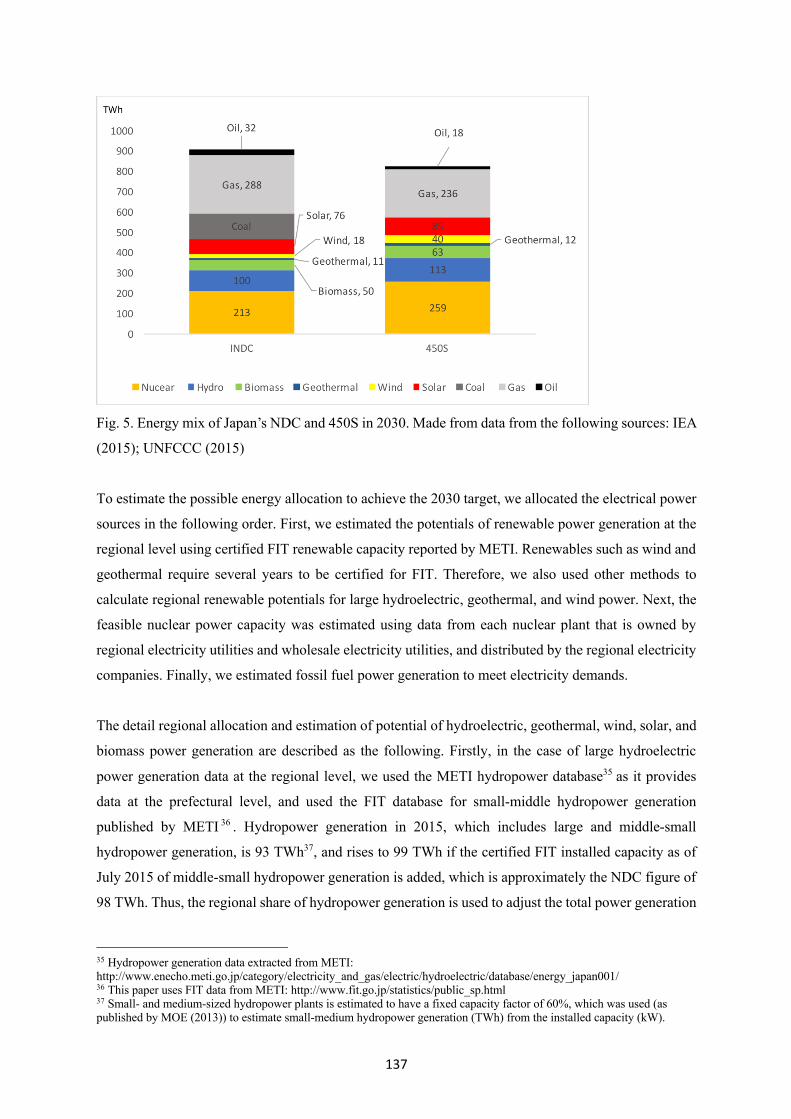
137

Fig. 5. Energy mix of Japan’s NDC and 450S in 2030. Made from data from the following sources: IEA

(2015); UNFCCC (2015)

To estimate the possible energy allocation to achieve the 2030 target, we allocated the electrical power

sources in the following order. First, we estimated the potentials of renewable power generation at the

regional level using certified FIT renewable capacity reported by METI. Renewables such as wind and

geothermal require several years to be certified for FIT. Therefore, we also used other methods to

calculate regional renewable potentials for large hydroelectric, geothermal, and wind power. Next, the

feasible nuclear power capacity was estimated using data from each nuclear plant that is owned by

regional electricity utilities and wholesale electricity utilities, and distributed by the regional electricity

companies. Finally, we estimated fossil fuel power generation to meet electricity demands.

The detail regional allocation and estimation of potential of hydroelectric, geothermal, wind, solar, and

biomass power generation are described as the following. Firstly, in the case of large hydroelectric

power generation data at the regional level, we used the METI hydropower database35 as it provides

data at the prefectural level, and used the FIT database for small-middle hydropower generation

published by METI 36 . Hydropower generation in 2015, which includes large and middle-small

hydropower generation, is 93 TWh37, and rises to 99 TWh if the certified FIT installed capacity as of

July 2015 of middle-small hydropower generation is added, which is approximately the NDC figure of

98 TWh. Thus, the regional share of hydropower generation is used to adjust the total power generation

35 Hydropower generation data extracted from METI: http://www.enecho.meti.go.jp/category/electricity_and_gas/electric/hydroelectric/database/energy_japan001/ 36 This paper uses FIT data from METI: http://www.fit.go.jp/statistics/public_sp.html 37 Small- and medium-sized hydropower plants is estimated to have a fixed capacity factor of 60%, which was used (as published by MOE (2013)) to estimate small-medium hydropower generation (TWh) from the installed capacity (kW).

138

to meet the NDC figure. For 450S, we used the FIT data, including the certified FIT data as of

September 2016 of 101.3 TWh. Because hydropower generation of 450S by 2030 is 113 TWh, we used

a share of the FIT data to meet 113 TWh.

Secondly, for the geothermal power generation capacity at the regional level38 , we used the data

obtained from the Japan Oil, Gas, and Metals National Corporation (JOGMNC),39 as well as the

company announcements of plans for public consultation to develop geothermal power plants40, and

then calculated the expected total installed capacity of geothermal power for 2030. Based on this, the

feasible geothermal power generation by 2030 is estimated at 10 TWh41,42. Japan’s NDC is 12 TWh for

geothermal power generation by 2030; thus, this paper adjusts the geothermal power generation to 12

TWh using a share of the regional capacity with an estimated 10 TWh regional capacity. Geothermal

power generation under 450S is the same as the figure for the NDC (i.e., 12 TWh).

Thirdly, for wind power generation, this study uses the installed capacity from FIT data, which results

in installed capacities of 13.6 TWh and 15.4 TWh for July 2015 and September 201643, including FIT-

certified capacity. Japan’s NDC targets 18 TWh of wind power generation by 2030; therefore, to

estimate the regional wind power generation by 2030 we used a share of the wind power generation

from the FIT data, including certified FIT by region, and adjusted the power generation to obtain 18

TWh in total. Wind power data estimated from METI (2011) reports are used for wind power generation

under 450S. Additionally considered was the project internal rate of return (PIRR)44 of potential

renewable electricity at the regional level. Wind power generation was based on an 8% PIRR after tax,

and a willingness to install wind power under an assumed FIT system. The analysis results indicated 43

TWh of onshore wind power generation, which is approximately the 450S expected wind power

38 In the case of geothermal projects, it takes more than ten years to move from the initial ground investigation to the start of actual operations: two years for the ground and excavation investigation, three years for exploration, three to four years for the environmental assessment, and three to four years for excavation of the production well and construction (METI, 2015a). Obtaining FIT approval for geothermal projects requires environmental assessments, among other procedures. Furthermore, if public discussion and coordination with local communities are needed, another five years may be required, meaning that a project designed to begin operation in 2030 should begin public consultations today; although this assumption may be too conservative. 39 Japan Oil, Gas and Metals National Corporation (JOGMNC) http://geothermal.jogmec.go.jp/ 40 There is no information on the anticipated installed capacity of geothermal power plants in public consultations, thus this study assumes sites located in hot spring areas at 500 kW (minimum installed capacity of medium-scale geothermal); those in national parks at 30,000 kW (large-scale geothermal is more than 15,000 kW); and others at 2,000 kW (maximum installed capacity of medium-scale geothermal). The data are based on a JOGMEC report (JOGMEC, 2013). 41 Includes sites in national parks. In October 2015, MOE announced eased regulations for parts of national parks, meaning development of geothermal power generation is possible for some sites (source: Asahi Shimbun newspaper (6 October 2015): http://www.asahi.com/articles/ASH7Z46TVH7ZULBJ005.html). 42 For geothermal electricity generation, we used a 70% capacity factor for installations of less than 5,000 kW, 75% for installations of 5,000–20,000 kW, and 80% for installations of more than 20,000 kW. Data from MOE (2013). 43 We used the capacity factor of average wind speed due to factor variations of 16.2% to 54% in speed (in metres per second), and 2,000 kW to 5,000 kW in capacity (METI, 2011). 44 PIRR is used to evaluate whether a project can be feasibly operated, and to determine whether the project will be successful or not. If PIRR is larger than the weighted average cost of capital (WACC), operation is usually feasible, with an expected return on investment. For instance, WACC is about 4.7–7.5% for onshore wind, and about 6.8–9.7% for offshore wind in some European countries and the USA (IEA, 2011).

139

generation of 40 TWh. Thus, we used the ratio of regional wind power capacity estimated in the METI

reports to the 450S power generation target.

In addition, for solar power generation, 33 TWh has already been installed, and the certified FIT solar

power in 2015 is 103 TWh (144 TWh as of September 2016). The NDC and IEA 450S targets are at 79

TWh and 85 TWh, respectively, which will be well covered by 136 TWh (33 TWh plus 103 TWh).

Thus, we considered the share of solar power as of July 2015. The surplus solar power capacity can be

used to replace fossil fuels; however, this study aims to identify barriers to the current electricity system

when the NDC and 450S renewables targets are achieved. Therefore, we used the targeted total power

generation by the NDC and 450S for the analysis.

Similarly, for biomass power generation, while Japan’s NDC for biomass is 49 TWh, the FIT power

generation estimated from the installed capacity is 27.5 TWh as of July 2015 and 38 TWh as of

September 201645,46. We thus take the share of regional biomass power generation as of September

2016 and estimate the power generation of 49 TWh by region. For 450S, biomass generation is expected

to be 63 TWh. In the absence of other data, we applied the share of regional biomass with the FIT power

generation as of September 2016, and apply it to NDC.

Additionally, to estimate the regional nuclear power generation by 2030, we first listed all existing

nuclear power plants47, then eliminated all plants that will have exceeded their 40-year operational

lifespans by 2030, which leaves only 2.4 MW of generation capacity. Total power generation in the

NDC and IEA are allocated to those remaining nuclear plants in each region. Yet, our detailed

examination on plant operation rates, and uncertainty on lifespan of plants reveals that the NDC and

IEA 450S nuclear targets will not be reachable. Hence, we used a more realistic national target in the

case of nuclear power. Even using a high operating ratio of 90% for nuclear, only 191.5 TWh could be

generated, which falls short of Japan’s NDC power generation target. The Nuclear Reactor Regulation

Law was amended in 2012 after the Fukushima nuclear accident, where, in principle, the maximum

operational lifespan of nuclear reactors was set to 40 years (Nawata, 2016). However, the regulation

also set up an exception to expand by additional 20 years with the approval of the Nuclear Regulation

Authority (NRA) (NRA, 2017). We, therefore, included the capacity of nuclear power from plants that

have exceeded their 40-year lifespan by 2030, which includes nuclear plants that have been restarted,

reactors restarted after passing the NRA conformity check, and newly approved revised nuclear power

45 A fixed capacity factor of 80% is used for biomass, as published by METI (2013b), to estimate the biomass electricity generation (TWh) from the installed capacity (kW). 46 The available biomass data published by NEDO is also 38 TWh in the total. http://app1.infoc.nedo.go.jp/biomass/index.html 47 We use the data from METI (as of February 2019): http://www.enecho.meti.go.jp/category/electricity_and_gas/nuclear/001/pdf/001_02_001.pdf

140

plant reactor installation as of February 2017. The total power generation from nuclear will be 217 TWh,

which is about the NDC target of 213 TWh.

However, that is the case when nuclear plants are operated with an operating ratio of 90%, which is

unrealistic. The estimated operating ratio by regional electricity utilities is around 70–85%48 (the

average capacity factor of nuclear power generation from 1990 to 2010 was 73.7%, with the highest

being 84.2% in 1998, and the lowest being 59.7% in 200349). Therefore, for the NDC, we included

plants that have not passed the NRA conformity check, or have not been approved for reactor

installation, but NRA conformity checks are underway. Further, they will not exceed their 40-year

lifespan by 2030. Therefore, nuclear power generation results in 214 TWh50– which is approximately

the NDC target – with the operating ratios published by regional electrical power companies. Based on

this data, we estimated the share of the regional nuclear power generation, and calculated the regional

nuclear power generations by 2030. For 450S, we included all existing nuclear power plants that have

not exceeded their 40-year lifespan by 2030. Thus, the total power generation from nuclear sources will

be 285 TWh using the operating ratios published by the regional electricity power companies, which

exceeds the 450S target of 259 TWh. With the share of the regional nuclear power generation data, the

expected total nuclear power generation of 259 TWh is allocated to regional nuclear electricity

generations. These estimates reveal that the targeted nuclear power generation for the NDC and 450S

is unrealistic and unachievable. Thus, this paper reports alternative energy sources to nuclear, and

consider the case to maximize the use of renewables within the targeted amount of renewable electricity

to replace nuclear to meet the NDC and 450S targets. Under the dispatch order where nuclear has first

priority order, some of renewables cannot be used, and are wasted even if it is generated.

For fossil fuels, we used survey data of existing and planned fossil fuel plants at the regional level, as

collected by the Ministry of Environment of Japan. To obtain regional figures for coal-fired, gas-fired,

and oil-fired power generation that agree with Japan’s NDC, we calculated the total power generation

of fossil fuel power plants that will not have exceeded their 40-year lifetimes by 2030, as well as fossil

fuel power plants planned to start operations before 2030, and then adjusted for the plant operation rate

to meet the NDC and 450S targets.

48 METI 2016. http://www.meti.go.jp/committee/sougouenergy/shoene_shinene/shin_ene/keitou_wg/pdf/009_08_01.pdf 49 FEPC database in 2016 extracted from: http://www.fepc.or.jp/library/data/infobase/ 50 For Hokkaido, Tohoku, Hokuriku, Chugoku, Shikoku and Kyusyu Electricity Power Companies, we use the data by METI 2016 (in Japanese) (the data is available: http://www.meti.go.jp/committee/sougouenergy/shoene_shinene/shin_ene/keitou_wg/pdf/009_08_01.pdf). For Tokyo, Chubu and Kansai Electricity Power Companies, the operating ratio is calculated by their historical operating ratios (Tokyo Electricity Power Company (EPCO): https://www4.tepco.co.jp/corporateinfo/illustrated/nuclear-power/nuclear-capacity-factor-j.html / Chubu EPCO: https://www.chuden.co.jp/energy/hamaoka/hama_jisseki/hama_setsubi/index.html?cid=ul_me / Kansai EPCO: http://www.kepco.co.jp/energy_supply/energy/nuclear_power/info/knic/library/unten/setubi.html)

141

Finally, we also collected data on the interconnection grid capacity, and the capacity of pumped

hydropower plants. For grid capacity, we used planned interconnection grid capacity data, including

heat capacity by 2030. For pumped hydropower plants, we used the electricity supply data as of 2015

obtained from METI51.

5.4. Results

Japan can reduce its carbon intensity from electricity generation to 0.29 kgCO2/kWh, which improves

from 0.55 kgCO2/kWh as of 2014 (Fig. 6-1), if Japan meets the following requirements; if renewables

can be generated to the level of Japan’s NDC target by 2030; if renewable electricity is generated in

based on the regional renewable capacity; if fossil fuel power generation is used to balance the

electricity demand and supply; and if the available cross-regional transmission capacity can be

maximised. In comparison, our analysis of the energy mix and carbon intensity is based on the

aggregated use of renewables to meet Japan’s NDC and 450S targets. It also considers a priority

dispatch order that the NDC target does not, which is as follows: baseload - renewables - biomass -

interconnection trade - fossil fuel power generation. As a result of this analysis, we find that the new

aggregated approach improves the carbon intensity of electricity more than the NDC target. The

voluntary emission intensity target suggested by power companies is 0.37 kgCO2/kWh (FEPC, 2015b).

The carbon intensity of 0.29 kgCO2/kWh can be achieved by replacing 18 TWh (NDC targets) and 26

TWh (IEA 450S targets) of fossil fuels to renewables.

The analysis also reveals that there is a huge reduction in emission intensity in Hokkaido, Tohoku,

Hokuriku, and Kyushu – all of which meet the nuclear and renewable potential for 2030, but have

relatively low electricity demand compared to other regions, especially highly populated areas like

Tokyo. Comparing the carbon intensity targets in the NDC, 450S, and 450S without nuclear reveals

that aggregating renewable power generation to the 450S level without nuclear will reduce Japan’s

carbon intensity to a level of 0.31 kgCO2/kWh, which is below that stated in the NDC target by

electricity companies (Fig. 6-2). Although the NDC without nuclear will exceed the carbon intensity

that stated in the NDC target, this paper reveals that Japan can increase more renewables than the NDC

target as described below, which will result in further reduction of carbon intensity from 0.41

kgCO2/kWh in the NDC target without nuclear. In the regional level, Hokkaido, Tohoku and Chubu

area have potentials to reduce carbon intensity even in case of no nuclear. Hokkaido has relatively high

carbon intensity in case without nuclear mainly because solar PV generation for the NDC target is

calculated by the share of solar power as of July 2015 when solar power in Hokkaido is still small

compared to their solar PV potentials in the area.

51 METI data: http://www.enecho.meti.go.jp/statistics/electric_power/ep002/results_archive.html

142

Fig 6-2. Estimated result of carbon intensity by region using demand and supply curve

Fig 6-1. Estimated result of aggregated carbon intensity in national level using demand and supply

curve. Made from the result of this paper. Source: FEPC 2015 for actual national carbon intensity in

2010 and 2014.*Fig.6-1 and Fig.6-2 shows the results of the calculated carbon intensity in 2030, which

was estimated considering nationwide aggregated management, flexible priority criteria, and hourly

precise control that is applied to the electricity system as a whole by introducing planned transmission

capacity towards 2030, and electricity system reform where the electricity can be traded across regions

by reforming the current ‘first-come-first-served’ grid transmission rule. Comparing with the NDC and

450S targets show that Japan can achieve the targeted carbon intensity if Japan reforms the electricity

market to enhance aggregated management, and introduce flexibility in the priority criteria, and in

transmission between regions.

The result of Japanese renewable potentials towards 2030 finds that enough renewable capacity exists

to fulfil requirements of the current plan. As for the possibilities of increasing renewables to the level

0.35

0.554

0.17

0.310.29

0.410.37

0

0.1

0.2

0.3

0.4

0.5

0.6

2010 2014 2030

Actual 450S(kgCO2/kWh) 450Swithoutnuclear(kgCO2/kWh) NDC(kgCO2/kWh)NDCwithoutnuclear(kgCO2/kWh) NDCtarget

0.5

0.44

0.34

0.34

0.38

0.3

0.24

0.18

0.18

0.13

0.387

0.303

0.261

0.222

0.176

0.173

0.128

0.036

0.021

0.003

0 0.1 0.2 0.3 0.4 0.5 0.6

Okinawa

Chugoku

Kansai

Tokyo

Shikoku

Chubu

Kyusyu

Tohoku

Hokuriku

Hokkaido

450S(kgCO2/kWh) NDC(kgCO2/kWh)

0.502

0.558

0.521

0.481

0.42

0.41

0.366

0.43

0.2

0.349

0.412

0.405

0.385

0.372

0.353

0.289

0.24

0.201

0.141

0.088

0 0.1 0.2 0.3 0.4 0.5 0.6

Okinawa

Chugoku

Shikoku

Kansai

Tokyo

Kyusyu

Chubu

Hokuriku

Tohoku

Hokkaido

450Swithoutnuclear(kgCO2/kWh) NDCwithoutnuclear(kgCO2/kWh)

143

of 450S, if we consider the latest FIT renewable data, the power generation from renewables in Japan

has already reached 147 TWh without large hydropower generation, as of February 201752. Including

both existing capacity and capacity under development, hydropower generation amounts to 241 TWh,

which approaches the NDC target of 256 TWh of renewables by 2030, making up 24% of the total

electricity generation. Furthermore, if certified FIT of renewables is included, it reaches about 300 TWh

of renewables, which the 450S target of 310 TWh for renewables. In addition, while solar PV in 450S

expects 79 GW, the installed capacity of renewables including certified FIT as of February 2017 has

already reached 121 GW.

On the other hand, although Hokkaido and Tohoku areas have large renewable potentials, these

potentials are not factored into the 2030 targets under the current electricity market system. (Fig. 7)

There are no incentives for investors to invest in these regions under a situation in which regional

electricity power companies individually set caps for generation capacities for solar and wind power

generation (SCJ, 2014). One of the challenges is the lack of power grid capacity. If new renewable

potentials are introduced in the regional level, it exceeds their electricity demand within the region.

Thus, the surplus power needs to be transferred to other regions. However, even if these renewables are

realised, there are issues in transmission to other regions through the interregional grid system, as well

as issues with storage within regions, which is needed to control supply (Buckley and Nichola, 2017).

52 METI large hydropower database (http://www.enecho.meti.go.jp/category/electricity_and_gas/electric/hydroelectric/database/energy_japan006/) METI FIT database (http://www.enecho.meti.go.jp/category/saving_and_new/saiene/statistics/index.html)

144

Fig. 7. Comparison of simulation results of power generation in 2030 and renewable potentials at the

regional level. Sources: Made from the following sources: Renewable potential (Wakiyama and

Kuriyama, 2015) and result of this paper

In addition, currently, nuclear power is prioritised as the baseload in the grid over renewables in all

regions. This is one of the barriers to accommodating more renewables in the regional supply. Hokkaido,

Tohoku, and Kyushu all have certain nuclear potentials, and the renewables must compete against them.

For instance, considering Tohoku in February – a time of relatively high electricity demand in the region

– nuclear maintains its relatively high ratio in the power supply under the NDC target (Fig. 8-1). Since

Tohoku satisfies its electricity demand by supply from within the region, the surplus of renewables

could be transmitted to the Tokyo area. However, when we considered a period when electricity demand

is low but supply from solar and wind is enough to meet regional demands, such as the generation of

up to 11 GWh between 13:00 and 14:00 on 12th April, the surplus is prevented from transmission to

the Tokyo area due to the limited cross-regional grid capacity of 7.3 GWh to transmit, as well as the

limited maximum grid capacity of 9.8 GWh53 for the renewable power capacity (Fig. 8-2). The 3 GWh

of renewables generated in Tohoku region is, therefore, neither consumed within the region, nor

53 This paper uses interregional grid connection data from 2016.

145

transferable to another region, and is, thus, wasted. Moreover, our analysis reveals that if nuclear is first

priority, even if renewables are second priority over fossil fuels, wind power generation potentially

exceeds the electricity supply required to meet the demand within region, and cannot transfer the surplus

power generated to other regions due to the limits of the transmission capacity. Surplus wind power

generated in Tohoku, Chubu, and Kyushu regions cannot be used, and is wasted. This surplus wind and

solar power could be used for compensating deficiency of total national power caused by over

estimation of nuclear capacity discussed earlier.

Fig. 8-1. Simulation results of demand and supply curve in Tohoku region for February 1–14

146

Fig. 8-2. Simulation results of demand and supply curve in Tohoku region for April 4–14. Made from

the result of this paper. *The figures above illustrate renewable generation potentials on different dates

in 2030, when Japan will have achieved the energy mix of the NDC target, which is estimated by

applying nationwide aggregated management, flexible priority criteria, and hourly precise control. As

an example, in Tohoku, the demand for electricity is relatively high in February due to it being winter,

and solar power generation is not large, supply does not exceed the regional demand (left figure). On

the other hand, in April, when the electricity demand is not too high due to spring season, and solar

power generation is higher, the total electricity supply within the region exceeds the demand, and the

renewables generated are transmitted to other regions (right figure).

Another finding is an oversupply, not only of renewables and nuclear, but also fossil fuels. This over

capacity of power generations comes from mismatches of government plans with established policies,

not from the new aggregated criterion. For fossil fuel power generation, current plans for new

constructions and replacements total 18 GW of coal-fired power plants, and 29 GW of natural gas-fired

power plants54, while the total capacities of existing plants are 49 GW, and 73 GW55, respectively. Even

if we exclude fossil fuel power plants that have exceeded their 40-year lifespan, the capacity is still

large compared to the NDC target. Coal, gas, and oil power generation are targeted at 277 TWh, 288

TWh, and 32 TWh in the NDC, respectively. Thus, to meet these targets, the existing plant operating

ratios must be approximately 90%, 59% and 50% for coal, gas, and oil, respectively, and if current

54 Agency for Natural Resources and Energy, “Standards for heat efficiency toward high efficiency thermal power plants” (17 November 2015), in Japanese 55 MOE, “Towards a large amount of GHG emission reduction in 2050” (11 October 2015), Agency for Natural Resources and Energy, “Standards for heat efficiency toward high efficiency thermal power plants” (17 November 2015), in Japanese.

147

plans for new constructions and replacements are included, these ratios will be 60%, 42% and 48%,

respectively. In the 450S, if current plans for new construction or replacement are carried out, the factor-

operating ratios will need to be reduced by 26%, 35% and 27%, for coal, gas, and oil, respectively. Our

analysis shows that in case the priority dispatch order is applied with priority of renewables over fossil

fuels, 248 TWh for coal, 300 TWh for gas, and 30 TWh for oil could be dispatched in the NDC scenario,

and 103 TWh for coal, 232 TWh for gas, and 15 TWh for oil in case of 450S. The operating ratios of

these fossil fuels would be further reduced. Although our analysis did not show the significant reduction

in coal power generation compared to the NDC target set by the government, it allocates high impact

to a coal-fired plant that already has a low operating ratio regarding economic feasibilities to

continuously operate the plants.

5.5. Discussion

To make economical use of renewables, the analysis results in section 4 point to a priority dispatch

order, and a cross-regional grid connection restructure as the keys to electricity market reform in Japan.

The analysis paints a picture of increasing competition between nuclear, renewables, and fossil fuels in

the context targets for 2030 and beyond, due to the issues of projected oversupply of power generation

and grid connection. Limited capacity of the grid, and the competition are, therefore, of the central

issues Japan needs to address; which means that it should clarify its stance on which technology should

be prioritised for power generation.

At the same time, the demand-response system could enhance the competition in electricity supply

among different electricity sources. The current electricity system reform is considering creating a

‘negawatt market’, which is aimed at reducing electricity demand. This would increase the competition

of electricity supply between nuclear and renewables. The establishment of a baseload electricity

generation market based on reform of the current electricity market, which is based on the idea that the

current retail market suffers from lack of liquidity due to domination by regional electricity companies

cheaply generating power from sources such as hydropower, biomass, nuclear, and geothermal (METI,

2017). Instigating such a market would facilitate access for non-utilities companies to trade in electricity.

However, the use of the baseload concept would be obviated in the case where a large renewable

capacity was expected, and renewables were to assume a bigger role in the context of a more flexible

market (Elliston et al 2012; Diesendorf 2007); or if renewables such as wind power were to act as a

baseload together with infrastructure for large-scale energy storage (Kempton and Tomić 2005; Al-

musleh et al2014). On the contrary, much attention has been globally focused in expanding potentials

of renewables by increasing reliability of the electricity grid system that currently prevents a large

fraction from renewables, especially solar and wind electricity, through a combination of electricity

148

storage system, and flexible market design, including demand response management (Denholm et al.,

2010; Lund et al., 2015; Zhong et al., 2015).

Other issues concerning the planned electricity market reform in Japan is the establishment of a non-

fossil fuel power market (electricity generated via non-fossil fuel sources including nuclear, hereinafter

referred to as “non-fossil fuel electricity”), which includes nuclear as a non-fossil fuel. This new scheme

aims to help reduce the present national burden of the renewable energy surcharge (METI, 2017).

Through the non-fossil fuel power market, non-fossil fuel electricity certificates (similar to renewable

portfolio standard (RPS) certificates) will be purchased by retail electricity companies willing to

increase the ratio of non-fossil fuel electricity in the total electricity supply (METI, 2017). Also aimed

at raising use of non-fossil fuel electricity is the Act on Sophisticated Methods of Energy Supply

Structures, established in 2011, and revised in 201656. The revision aims to increase the ratio of non-

fossil fuel electricity generated by retail electricity power companies, with electricity supplies of over

0.5 TWh to over 44% by 2030 as part of Japan’s NDC goal (26% reduction in greenhouse gas emissions

between 2013 level by 2030)57 (Ogasawara, 2016). Furthermore, electrical power companies have set a

target emission of 0.37 kgCO2/kWh in their energy mix (JAPC, 2015). However, this raised an issue

because non-fossil fuel includes nuclear, and viewed in terms of the baseload market, nuclear will be

traded in two different markets. As discussed in section 4, competition exists between nuclear and

renewables under such circumstances, and nuclear has the priority over renewables. This paper reveals

that if Japan can increase renewables electricity generation reduce the electricity demands more than

the government NDC target up to the IEA 450S level and, Japan could satisfy the electricity demands

without nuclear supply. After the Fukushima nuclear accident, it reveals that the external costs of

nuclear has been dramatically increased due to the compensation and recovery costs from the disaster

as well as the decomposition costs.

5.6. Limitations of this study

The limitations of the method applied in this paper are as follows. First, the model employed applies

only to an electricity supply trend for each electricity generation source, i.e., wind and solar power; in

actual systems, renewable energy supply would be more complex due to differences in trends and

locations. Second (although this issue chiefly affects only Hokkaido and Tohoku), this model does not

calculate the level of wind power curtailment needed to satisfy the supply-demand balance. Third, the

impact of the diminishing cost of solar PV and wind power generation over time was not accounted for.

In fact, solar power technology has developed much more rapidly than predicted in several earlier

studies since the current solar capacity of Japan was installed (METI, 2014). Fourth, the model used

56 METI 2016: http://www.meti.go.jp/committee/sougouenergy/denryoku_gas/kihonseisaku/pdf/004_05_00.pdf 57 METI 2015 http://www.meti.go.jp/committee/sougouenergy/denryoku_gas/kihonseisaku/pdf/002_06_00.pdf

149

for analysis of the electricity system needs updating to better reflect the actual situation in which

electricity is supplied via several different sources. In addition, increase in costs by introducing

renewables, and necessary investment for transmission are not considered. Finally, this study also does

not consider one of the government objectives to ‘suppress electricity rate’. These will be addressed

next.

5.7. Conclusions and Policy Implications

This study examined the feasible CO2 emission intensity by 2030 under the current electricity system

of limited transmission network capacity, and the government plans for electricity market reform

towards 2020. It draws inferences to realise more renewable potentials. We found that, depending on

the region, Japan has the potential to increase renewable energy and improve the carbon intensity

reduction target stated in Japan’s NDC. Improved grid-interconnectedness and system reform are all

required, which necessitate the introduction of the priority order system, which ranks available sources

of energy in the order of their short-run marginal costs of production, for bringing the sources with the

lowest marginal costs online to meet demands before the higher cost sources, and expanding the

capacity of the grid system. If Japan can generate renewables by maximising the use of regional

renewable potentials, they can meet and exceed the carbon intensity reduction target of the electricity

sector and the NDC target without using nuclear power. The currently discussed electricity market

reform, which covers the baseload market and non-fossil fuel power market, is neither an efficient, nor

effective mechanism in terms of increasing renewable energy if surplus of electricity generation among

nuclear, renewable, and fossil fuels is expected towards 2030 and beyond. A further issue related to

both the current and future markets regarding fossil fuels is that if Japan and the rest of the world aim

to achieve the 2DS pledged under the Paris Agreement, supply exceeds the demand due to the increase

in renewable energy, and fossil fuels will be in oversupply.

Therefore, to electricity market reform, Japan needs to reconsider building additional fossil fuel plants

by strengthening governmental regulations, while considering ways to replace these power plants to

renewables by 2030 in a cost-effective way. For this, renewables need political support and systems to

operate priority dispatch order over nuclear power generation towards the electricity reform in 2020,

and to attract the investment in renewables.

However, the main challenges in implementing electricity reform policies to promote renewables is that

Japan still considers nuclear as cheap baseload electricity. While current climate policies intended to

achieve the climate target of the NDC, the nuclear potentials towards 2030 are not realistic under current

conditions considering their feasibility in terms of the life spans, and the restarting operation of nuclear

plants. The accumulating costs and government spending for recovering from Fukushima nuclear

150

accidents has increased the uncertainties of the lifetime costs of nuclear power plants. Hence, Japan

needs alternative electricity sources, and redirection of governmental budgets from nuclear to

renewables. Renewables can maximise generation with a combination of technologies and policies by

promoting flexible grid operation, strengthening transmission capacity, and prioritising renewables in

the dispatch order. In addition, local and central governments can consider maximising renewable

potentials by supporting investments in technology for stabilising electricity systems supplied by

renewable electricity, such as pumped storage hydropower, storage cells, and demand-response that can

store surplus energy until needed.

151

5.8. References

Adachi, T. (1981). Basic Study of Estimadon Method of Wind Speedbelow150m byPower Law.

Japan Weather Associatoin, 28(4), 42–50.

Al-musleh, E. I., Mallapragada, D. S., & Agrawal, R. (2014). Continuous power supply from a

baseload renewable power plant. Applied Energy, 122, 83–93.

https://doi.org/10.1016/j.apenergy.2014.02.015

Aoyama, H. (2017). Current Situation and Issues of Electricity System Reform: Focusing on Full

Retail Competition (Japanese). Issue Brief, National Diet Library (Vol. 942).

Bahar, H. and J. S. (2013). Cross-Border Trade in Electricity and the Development of Renewables-

Based Electric Power: Lessons from Europe. OECD Trade and Environment Working Papers,

2013/02, OECD Publishing, Paris. Retrieved from http://dx.doi.org/10.1787/5k4869cdwnzr-en

Blazejczak, J., Braun, F. G., Edler, D., & Schill, W. P. (2014). Economic effects of renewable energy

expansion: A model-based analysis for Germany. Renewable and Sustainable Energy Reviews,

40, 1070–1080. https://doi.org/10.1016/j.rser.2014.07.134

Buckley, T., & Nichola, S. (2017). Japan: Greater Energy Security Through Renewables Electricity

Transformation in a Post-Nuclear Economy. The Institute for Energy Economics and Financial

Analysis (IEEFA). Retrieved from http://ieefa.org/wp-content/uploads/2017/03/Japan_-Greater-

Energy-Security-Through-Renewables-_March-2017.pdf

DDPP. (2015). Deep Decarbonization Pathways. Synthesis Report, SDSN - IDDRI. Retrieved from

http://unsdsn.org/what-we-do/deep-decarbonization-pathways/

DeMarrais, Gerard, A. (1958). Wind-Speed Profiles at Brookhaven Nantional Laboratory. Journal of

Meteorology, 16, 181–190.

Denholm, P., Ela, E., Kirby, B., & Milligan, M. (2010). Generation, Role of Energy Storage with

Renewable Electricity. National Renewable Energy Laboratory, Technical Report NREL/TP-

6A2-47187.

Diesendorf, M. (2007). The Base-Load Fallacy. ANZSEE Solar Conference, 1–7.

EEC. (2012). Innovative Strategy for Energy and the Environment (provisional translation). 14

September 2012: Energy and Environment Council, the Government of Japan.

Elliston, B., Diesendorf, M., & MacGill, I. (2012). Simulations of scenarios with 100% renewable

electricity in the Australian National Electricity Market. Energy Policy, 45, 606–613.

https://doi.org/10.1016/j.enpol.2012.03.011

ETRA. (2014). Basic Principle of Electric Utility (Japanese). Electric Technology Research

Association. Retrieved from http://www.etra.or.jp/concept/etra_concept_faq.pdf

FEPC. (2015a). Electricity Review Japan.

FEPC. (2015b). Environmental Action Plan in the Electricity Business 2015 (Japanese).

Froggatt, A., & Schneider, M. (2015). Nuclear power versus renewable energy - A trend analysis.

152

Proceedings of the IEEE, 103(4), 487–490. https://doi.org/10.1109/JPROC.2015.2414485

GOJ. (2011). Act on Special Measures Concerning Procurement of Electricity from Renewable

Energy Sources by Electricity Utilities (Japanese).

Huenteler, J., Schmidt, T. S., & Kanie, N. (2012). Japan’s post-Fukushima challenge – implications

from the German experience on renewable energy policy. Energy Policy, 45, 6–11.

https://doi.org/10.1016/j.enpol.2012.02.041

Ichinosawa, M., Sawa, T., Tanaka, H., Fujiwara, S., & Nishioka, A. (2016). Solutions for changes to

cross-regional grid operation improving from electricity system reform. Hitachi Review, 65(4),

911–919.

IEA. (2011). IEA Wind Task 26. Wind Energy, 1–122. Retrieved from

http://www.nrel.gov/docs/fy11osti/48155.pdf

IEA. (2015). World Energy Outlook. https://doi.org/10.1787/weo-2014-en

Inoue, M., Genchi, Y., & Kudoh, Y. (2017). Evaluating the Potential of Variable Renewable Energy

for a Balanced Isolated Grid: A Japanese Case Study. Sustainability, 9(1), 119.

https://doi.org/10.3390/su9010119

JAPC. (2015). Implementation Plan of Electric Power for a Low Carbon Society (Japanese). The

Japan Atomic Power Company. Retrieved from

http://www.japc.co.jp/news/press/2015/pdf/270717.pdf

JOGMEC. (2013). Handbook for promotion of hot spring power generation introduction of the small-

scale geothermal power generation (Japanese). Retrieved from

http://geothermal.jogmec.go.jp/data/file/023.pdf

Jones Day. (2013). Renewable Energy In Japan : One Year After The Implementation of the Feed-in

Tariff Law. Jones Day Commentary, (August), 1–2.

Karakosta, C., Pappas, C., Marinakis, V., & Psarras, J. (2013, June 1). Renewable energy and nuclear

power towards sustainable development: Characteristics and prospects. Renewable and

Sustainable Energy Reviews. Pergamon. https://doi.org/10.1016/j.rser.2013.01.035

Keay, M., Rhys, J., & Robinson, D. (2012). Decarbonization of the electricity industry – is there still a

place for markets ? Oxford Institute for Energy Studies, 286084(November). Retrieved from

https://www.oxfordenergy.org/wpcms/wp-content/uploads/2012/11/EL-9.pdf?v=6cc98ba2045f

Kempton, W., & Tomić, J. (2005). Vehicle-to-grid power implementation: From stabilizing the grid

to supporting large-scale renewable energy. Journal of Power Sources, 144(1), 280–294.

https://doi.org/10.1016/j.jpowsour.2004.12.022

Komiyama, R., & Fujii, Y. (2014). Assessment of massive integration of photovoltaic system

considering rechargeable battery in Japan with high time-resolution optimal power generation

mix model. Energy Policy, 66, 73–89. https://doi.org/10.1016/j.enpol.2013.11.022

Komiyama, R., & Fujii, Y. (2017). Assessment of post-Fukushima renewable energy policy in Japan ’

s nationwide power grid, 101(May 2016), 594–611.

153

Kuwahara, H. (2015). Electricity Network Investment and Competition Policy For a Low Carbon

Future (Japanese). Journal of Economics of Kwansei Gakuin University, 69(1), 133–163.

Lund, P. D., Lindgren, J., Mikkola, J., & Salpakari, J. (2015). Review of energy system flexibility

measures to enable high levels of variable renewable electricity. Renewable and Sustainable

Energy Reviews, 45, 785–807. https://doi.org/10.1016/j.rser.2015.01.057

METI. (2011). Research report on New Energy promotion basic research: Survey on installed

capacity of wind energy (Japanese). Retrieved from

http://www.meti.go.jp/meti_lib/report/2011fy/E001771.pdf

METI. (2012). Interim report on the masterplan for reinforcement of interconnection capacity. Study

on strengthening of interconnected transmission lines under the technichnology (Japanese).

Retrieved from

http://www.meti.go.jp/committee/sougouenergy/sougou/chiikikanrenkeisen/report01.html

METI. (2013a). New Energy promotion basic research: Survey on power use and heat utilization by

biomass and waste (Japanese). Retrieved from

http://www.meti.go.jp/meti_lib/report/2013fy/E002702.pdf

METI. (2013b). The Policy on Electricity System Reform. Cabinet decision. Retrieved from

http://www.meti.go.jp/english/press/2013/pdf/0402_01a.pdf

METI. (2014). Recent solar power market trends (Japanese), 0–38. Retrieved from

http://www.meti.go.jp/committee/chotatsu_kakaku/pdf/013_02_00.pdf

METI. (2015a). Introduction of renewable energy of each power supply (Japanese), 0–42.

METI. (2015b). Reinforcement of interconnection capacity: Power supply and demand verification

subcommittee (Japanese). https://doi.org/10.1007/s13398-014-0173-7.2

METI. (2017). Policy subcommittee for implementation of power system reform: Interim summary

(Japanese). Retrieved from

http://www.meti.go.jp/committee/sougouenergy/denryoku_gas/denryoku_gas_kihon/pdf/002_05

_02.pdf

MOE. (2013). Report on renewable energy zoning basic information (Japanese). Retrieved from

https://www.env.go.jp/earth/report/h26-05/index.html

Muhammad-Sukki, F., Abu-Bakar, S. H., Munir, A. B., Mohd Yasin, S. H., Ramirez-Iniguez, R.,

McMeekin, S. G., … Mat Tahar, R. (2014). Feed-in tariff for solar photovoltaic: The rise of

Japan. Renewable Energy, 68, 636–643. https://doi.org/10.1016/j.renene.2014.03.012

Nawata, Y. (2016). 40-year rule for Japan’s nuclear reactors and its challenges (Japanese). House of

Councilors, Research and Legislative (Vol. 381).

Neuhoff, K., Ruester, S., & Schwenen, S. (2015). Power Market Design Beyond 2020: Time to Revisit

Key Elements? DIW Berlin Discussion Paper No. 1456. Retrieved from

ssrn.com/abstract=2576693 or http://dx.doi.org/10.2139/ssrn.2576693

NIES. (2010). Japan Roadmaps towards Low-Carbon Societies: Towards the 80 per cent reduction of

154

CO2 emissions in 2050.

NRA. (2017). Cabinet decision: "A draft amending law on nuclear material substances, nuclear fuel

materials and nuclear reactor regulations to strengthen safety measures in nuclear power use

(Japanese). Nuclear Regulation Authority.

OCCTO. (2017). Organization for Cross-regional Coordination of Transmission Operators, JAPAN

Annual Report ‐Fiscal Year 2016.

Ogasawara, J. (2016). Developments in the Electricity Market. The Institute of Energy Economics,

Japan.

Ogimoto, K., Kataoka, K., Ikegami, T., Nonaka, S., Azuma, H., & Fukutome, S. (2014). Demand-

supply balancing capability analysis for a future power system. Electrical Engineering in Japan

(English Translation of Denki Gakkai Ronbunshi), 186(2), 21–30.

https://doi.org/10.1002/eej.22488

Pfenninger, S., & Keirstead, J. (2015). Renewables, nuclear, or fossil fuels? Scenarios for Great

Britain’s power system considering costs, emissions and energy security. Applied Energy, 152,

83–93. https://doi.org/10.1016/j.apenergy.2015.04.102

Roth, M. B., & Jaramillo, P. (2017). Going nuclear for climate mitigation: An analysis of the cost

effectiveness of preserving existing U.S. nuclear power plants as a carbon avoidance strategy.

Energy, 131, 67–77. https://doi.org/10.1016/J.ENERGY.2017.05.011

SCJ. (2014). Report: Toward expansion of usage of renewable energy (Japanese). Science Council of

Japan.

Sovacool, B. K. (2010). A Critical Evaluation of Nuclear Power and Renewable Electricity in Asia.

Journal of Contemporary Asia, 40(3), 369–400. https://doi.org/10.1080/00472331003798350

Tsuchiya, H. (2012). Electricity supply largely from solar and wind resources in Japan. Renewable

Energy, 48, 318–325. https://doi.org/10.1016/j.renene.2012.05.011

UNFCCC. (2015). Japan’s Intended Nationally Determined Contribution. Retrieved from

http://www4.unfccc.int/submissions/INDC/Published Documents/Japan/1/20150717_Japan’s

INDC.pdf

Vázquez, C., Rivier, M., & Pérez-Arriaga, I. J. (2002). A market approach to long-term security of

supply. IEEE Transactions on Power Systems, 17(2), 349–357.

https://doi.org/10.1109/TPWRS.2002.1007903

Vivoda, V. (2012). Japan’s energy security predicament post-Fukushima. Energy Policy, 46, 135–

143. https://doi.org/10.1016/j.enpol.2012.03.044

Vivoda, V. (2016). Energy Security in Japan: Challenges After Fukushima (Transforming

Environmental Politics and Policy). Routledge.

Wakeyama, T. (2016). System operation to introduce the expansion of renewable energy: Comparison

of Japan and Europe (Japanese). Natural Energy Foundation.

https://doi.org/10.1017/CBO9781107415324.004

155

Wakeyama, Tatsuya, & Ehara, S. (2011). Estimation of Renewable Energy Potential and Use: A Case

Study of Hokkaido; Northern-Tohoku Area and Tokyo Metropolitan; Japan. World Renewable

Energy Congress – Sweden, 12(057), 3090–3097. https://doi.org/10.3384/ecp110573090

Wakiyama, T., & Kuriyama, A. (2015). Can Japan Improve on its INDC-based Target for CO 2

Intensity in the Electricity Sector? Estimation of Renewable Electricity and Nuclear Power in

2030. IGES/OCN Working Paper.

Wilson, N., Palmer, K. L., Palmer, K., & Burtraw, D. (2005). The Impact of Long-Term Generation

Contracts on Valuation of Electricity Generating Assets under the Regional Greenhouse Gas

Initiative, (August).

Zhong, H., Xia, Q., Xia, Y., Kang, C., Xie, L., He, W., & Zhang, H. (2015). Integrated dispatch of

generation and load: A pathway towards smart grids. Electric Power Systems Research, 120,

206–213. https://doi.org/10.1016/j.epsr.2014.04.005

156

5.9. Appendix

Estimation of Electricity Supply to the Electric Grid System

This Appendix provides procedures to estimate electricity supply to an electric grid system in all regions

as a whole. As calculation of electricity supply and demand for each hour, an hourly basis electricity

supply and demand were calculated by the following equations:

Demand

𝑑=E>E,7 =𝐷=E>E ∗F"#$%,'

∑ F"#$%,'('

(eq. A7-1)

Where

i: time of electricity demand

n: total number of hours in a year (8,760)

𝐷=E>E,7 : Electricity demand for each grid for all power plants including distribution losses in 2030

(kWh)

𝑑=E>E,7 : Electricity demand at hour i in 2030 (kW)

𝑑=E*,,7 : Electricity demand at hour i in 2014 (kW)

Nuclear

𝑒H,7 =𝐸H/8760 (eq. A7-2)

Where:

𝑒H,7: Electricity supply capacity by nuclear power (kW)

𝐸H,7: Potential electricity supply in 2030 by nuclear power (kWh)

Hydro

𝑒4,7 =𝐸4/8760 (eq. A7-3)

Where:

𝐸4,7: Potential electricity supply in 2030 by hydropower (kWh)

Biomass

𝑒I,7 =𝐸I/8760 (eq. A7-4)

Where:

𝐸I,7: Potential electricity supply in 2030 by biomass power (kWh)

Geothermal

𝑒J,7 =𝐸J/8760 (eq. A7-5)

Where

157

𝐸J,7: E Potential electricity supply in 2030 by geothermal power (kWh)

Fossil fuels

𝑒KI,7 =𝐸KI/8760 (eq. A7-6)

Where

𝐸KI,7 : Electricity supply in 2030 to be used to adjust supply and demand (kWh)

Solar power

𝑒$,7 =𝐸$,7 ∗"'

∑ "'('

𝑟7 =∑ "',)*)

L

Where

i: time of electricity supply

j: monitoring points


m: total number of AMeDAS monitoring points

𝐸$,7: Potential electricity supply in 2030 by solar power (kWh)

𝑟7,1 : Solar radiation (MJ/m2)

Wind power:

𝑣ME7,1 =𝑣*E,7,1 'ME*E-N'

(eq. A7-7)

𝑓7,1 = 𝛼𝑣ME> 7,1 if𝑣 ≤ 14

𝑓7,1 = 𝛼(14)ME> 7,1 if14 < 𝑣 ≤ 25 (eq. A7-8)

𝑓7,1 = 0if25 < 𝑣

𝑓7 =∑ O',)*)

L (eq. A7-9)

𝑒P7 =𝐸$ ∗O'

∑ O'('

(eq. A7-10)

Where;

i: time of electricity supply

j: monitoring points that located at the place where wind power potential is observed


m: total number of AMeDAS monitoring points

𝐸P7 : Potential electricity supply in 2030 by wind power (kWh)

𝑓7,1 : Wind force at 80m height

158

𝑣*E,7,1 : Wind speed at 10m height

𝑣ME,7,1 : Wind speed at 80m height

𝛼 : Correction factor

𝛽7 : Power exponent for each i, determined in the table below

Hour 0 1 2 3 4 5 6 7 8 9 10 11

𝛽 0.3 0.3 0.3 0.3 0.3 0.3 0.3 0.3 0.3 0.2 0.1 0.05

Hour 12 13 14 15 16 17 18 19 20 21 22 23

𝛽 0 0 0 0 0 0.05 0.1 0.2 0.2 0.25 0.3 0.3

Source: DeMarrais (1958); Adachi (1981)

159

Chapter 7

Conclusion

The research presented in this thesis introduced tools to conduct sustainability analysis at a subnational

level. These analytical tools could help government and businesses assess CO2 emissions throughout

supply chains (Chapters 2 to 4) and identify the reduction potential for emissions generated from

electricity (Chapters 5). Indirect GHG emissions are generated through all associated activities in

supply chains. On the other hand, GHG emissions are generated directly from fuel combustion,

company vehicles, and fugitive emissions, as well as indirectly from consumption of purchased

electricity, heat, or steam. Cities and companies are the main actors to mitigate GHG emissions by

identifying reduction opportunities, tracking performance, and engaging suppliers. Understanding

environmental and social issues at the subnational level is key in designing policy aimed at mitigating

the direct and indirect impacts of a city economy on sustainability.

This thesis is novel in its introduction of two tools to assess sustainability. The tools are applied to

various research, such as the construction of a subnational MRIO table, which is time- and labour-

intensive for researchers. By using the tool (Japan IELab) introduced in Chapter 2, researchers can

conduct city-level and business-level impact analyses in a timely manner. The tools can also be used to

create indicators to measure sustainability in various areas of study. Further, the thesis addresses the

importance of the tools to assess the sustainability of various economic activities. It introduces research

findings that enhance the transparency of these human activities, such as supply chains, and trace its

environmental impacts through the use of the tools.

Micro- and macro-analytical tools were used for the sustainability analysis. Using the micro-analytical

tool, a bottom-up technology analysis was conducted, and the following issues were addressed: how

regional renewable energy potential can be put to effective use; how electricity reform both capitalized

on renewables and reduced carbon intensity; and how to structure and sequence electricity market and

climate policy reforms in an effort to cut CO2 emissions. The regional energy-mix potentials for

maximized renewable-electricity generation and reduced CO2 emission intensity in the electricity sector

should be identified to reduce environmental burdens such as CO2 emissions at the regional level within

a country. On the other hand, using macro-analytical tools such as IO and hybrid IO method, cities and

business should monitor the progress of reducing their GHG emissions across the whole supply chain.

The Japan MRIO database introduced in this thesis can be used to track and assess city-level emissions

160

throughout supply chains within Japan. It also has further potential to assess various social,

environmental, and economic problems—not only GHG emissions. For instance, the food loss

footprints at the regional level are identified and quantified from both a production perspective (the

producers’ responsibility) and a demand-side perspective (the consumers’ responsibility). Another

promising application for the MRIO database is in disaster impact management that considers regional

supply chains. To respond adequately to such disasters and the economy-wide shocks that they produce,

it is crucial for researchers and policymakers to assess the impact of these external shocks on critical

supply chains in a timely manner. Such assessments can be made using a high-resolution MRIO system

that provides information on transactions between the various sectors of the economy and the regions

in a country. The city-level MRIO table appropriately characterizes various economic activities and

accurately reflected the locational features of a city. In this thesis, it is also clarified that IO databases

and associated calculus are required for city footprint analyses to avoid severe errors that arise from

unacceptable scope limitations caused by the truncation of the footprint assessment boundary.

In future work, Japan’s city-level MRIO database should be linked to a global database, so that global

supply chains can be analyzed. To cover all supply chains, the linkage is crucial. This would enable,

for instance, an analysis of how production of a specific product or the consumption of a specific good

in one city in Japan affects the economy and environment of a region or city elsewhere in the world. To

this end, we intend to link the Japan IELab with the IELab family (Australia, China, Indonesia, and

Global) and to use this linkage to conduct a comprehensive analysis of trade among countries.