metode regulacije ep primenom mikroprocesora - skripta

of 52 Metode regulacije EP primenom mikroprocesora- skripta

Metode regulacije energetskih pretvarača primenom mikroprocesora

- skripta -

Darko Marcetic, Ph.D.

Rev Date DCO Originator Description X1 10/17/09 --- dr Darko Marcetic First draft

TABLE OF CONTENTS

1. Uvod u vektorsko upravljanje AM .................................................................................................... 3

2. Matematički model asinhronog motora........................................................................................ 5

2.1. Matematički model u originalnom abc domenu .................................................................. 5

2.2. Korišćene transformacije koordinata ....................................................................................... 6

2.3. AM model u αβ domenu..................................................................................................................... 9

2.4. IM model in dq reference frame .................................................................................................. 9

3. Indirektna vektroska kontrola (IFOC) ........................................................................................ 11

3.1. Strujno kontrolisani naponski invertor – redukcija reda AM modela .................. 11

3.2. IFOC – Teorijske osnove, analogni domen .......................................................................... 14

3.3. IFOC – Praktična implementacija (preview) ...................................................................... 15

4. Merenje linijskih struja motora....................................................................................................... 17

5. Merenje položaja rotora inkrementalnim enkoderom ....................................................... 20

5.1. Procena brzine rotora na osnovu merenog položaja ..................................................... 22

6. Space vector PWM modulator (SVPWM) for VSI................................................................... 24

6.1. Introduction ........................................................................................................................................... 24

6.2. Space Vector reference – Inverse Park ................................................................................. 24

6.3. Space vector theory .......................................................................................................................... 24

6.4. Space Vector Pulse-Width Modulation (SVPWM) ............................................................ 27

6.5. Software implementation notes for SVPWM....................................................................... 30

7. Motor current regulators in dq reference frame ................................................................... 32

7.1. Motor phase currents from measured line currents ...................................................... 32

7.2. Motor phase currents from abc to dq frame ....................................................................... 33

7.3. Typical digital current control model ...................................................................................... 33

7.4. Incremental dq current regulators with output limits ................................................. 34

7.5. Current regulators parameters evaluation .......................................................................... 36

8. Discrete IFOC control ............................................................................................................................ 38

of 52 Metode regulacije EP primenom mikroprocesora- skripta 8.1. IFOC overview ...................................................................................................................................... 38

8.2. Implementation of discrete IFOC equations ...................................................................... 38

8.3. Simplified block diagram of IFOC control algorithm...................................................... 41

8.4. IFOC – quasi C-code implementation ..................................................................................... 41

9. Speed regulator ........................................................................................................................................ 42

9.1. Speed regulator parameters calculation procedure....................................................... 42

9.2. Maximum Q phase current calculation – current limit ................................................. 42

10. Field weakening – flux control ........................................................................................................ 42

11. Induction motor parameters and data ....................................................................................... 43

11.1. Initial Induction motor parameters and data ............................................................... 43

12. Influence of Tr parameter error on IFOC .................................................................................. 44

12.1. Dobro odabran paramater Tr*= Tr ...................................................................................... 44

12.2. Pogrešno odabran paramater Tr*≠≠≠≠ Tr ................................................................................ 44

13. Signal data ranges for 12-bit ADC................................................................................................ 47

13.1. DC bus voltage measurement................................................................................................. 47

13.2. Inverter leg current measurement...................................................................................... 48

14. Appendix- Motor phase voltage and currents......................................................................... 49

14.1. Motor phase windings connected in the wye connection ...................................... 50

14.2. Motor phase windings connected in the delta connection .................................... 50

14.3. Phase voltages and currents in ααααββββ coordinate system ............................................. 51

14.4. Phase voltages and currents in dq coordinate system ............................................ 52


1. Uvod u vektorsko upravljanje AM U svim električnim pogonima sa promenjivom brzinom (Sl. 1.1) je poželjno imati pogon koji se ponaša kao aktuator momenta, t.j. u kome se skoro trenutno može razviti momenat jednak zadatoj vrednosti. Time se dinamika električnog dela sistema potpuno razdvaja i ne utiče na dinamiku mehaničkog dela i upravljanje brzinom i položajem je u takvim sistemima znatno uprošteno.

Fig. 1.1. Pogon motora sa promenjivom brzinom

Pogon motora jednosmerne struje, prikazan sa povratnom spregom po brzini, Sl. 1.2, predstavlja idealan konvertor momenta zato što su statorsko i rotorsko polje uvek normalni jedno na drugo i bilo kom trenutku. Uz konstantno polje statora, razvijeni momenat je moguće linearno regulisati promenom struje rotora i time se dobija optimalna dinamička karakteristika pogona.

Fig. 1.2. Speed control block diagram of the DC drive.

U slučaju asinhronog motora, koji je jeftiniji, robusniji i lakši za održavanje od jednsomernog motora, linearna kontrola momenta je moguća samo primenom raznih kompleksnih algoritama upravljanja, poznatih kao kontrola orijentacije polja (FOC -field oriented control) . Ima više vrsta ove kontrole: orijentacija ka fluksu statora, ka fluksu rotora i ka fluksu u međugvožđu. Postoje i dve osnovne metode upravljanja fluksom , direktna i indirektna. Tokom ovog kursa uglavnom ćemo se zadržati na indirektnoj vektorskoj kontroli (IFOC - indirect rotor field oriented control). Osnovni princip FOC upravljanja se može razumeti preko strujne konture koja se nalazi u konstantnom polju fluksa, kao što je prikazano na sl. 1.3. Momenat koji deluje na strujnu konturu iznosi: θψ sin⋅⋅= iTe

Gde je ψ amplituda fluksa kroz konturu (proizvod indukcije -B, i površine konture -S, i broja navojaka konture -N), i je veličina struje, i θ je ugao između vektora fluksa i vektora struje (normalan na površinu strujne konture i u smeru fluksa koji se pravi od te struje). Očigledno, maksimalni momenat se dobija kada je strujni vektor normalan na polje fluksa.


Fig. 1.3. Momenat koji deluje na strujnu konturu

Dakle, da bi se ostvarilo optimalno upravljanje asinhronim motorom neophodno je nezavisno upravljati fluksom i ostvarenim elektromagnetnim momentom.Konture upravljanja ovim veličinama se mogu razdvojiti regulacijom amplitude magnetopobudne sile statora i njenog relativnog položaja u odnosu na vektor fluksa rotora. Magnetopobudnu silu statora je moguće regulisati strujno regulisanim naponskim invetorom (CRVSI-current regulated voltage source inverter). Položaj fluksa rotora se proračunava algoritmom indirektne vektorske kontrole (IFOC–indirect filed oriented control). Po ovom algoritmu procena položaja se vrši u strujnom modelu rotorskog kola koji na osnovu vektora struje statora i mehaničkog položaja rotora simulira pojave u rotoru motora. Blok šema tipičnog IFOC pogona sa davačem položaja na vratilu data je na slici 2.4.

Regulacioni sistem

Strujno regulisani naponski invertor

M 3~

θr

Davač položaja

PI reg.

procena položaja rotorskog fluksa

Reference fluksa i momenta

dq abc

dq abc

id

iq

id*

iq*

vd*

vq*

Vabc*

Iabc

Vdc

Va

Vb

Vc

θdq

V~

θdq

Sl. 1.4. Šematski prikaz vektorski kontrolisanog asinhronog motora sa

strujno regulisanim naponskim invertorom. ŠTA JE ZADATAK PRI VEKTORSKOM UPRAVLJANJU AM?

• Primiti komande željene amplitude rotorskog fluksa i željenu vrednost el. momenta

• proceniti položaj vektora rotorskog fluksa • utisnuti u stator vektor struje takve amplitude i ugla da se ostvare zadati fluks i

momenat


2. Matematički model asinhronog motora

2.1. Matematički model u originalnom abc domenu Matematički model asinhrone mašine se sastoji od diferencijalnih i algebarskih jednačina, kojima se opisuju elektromagnetne (električni podsistem) i mehaničke pojave (mehanički podsistem) u mašini. Model električnog podsistema može se dobiti na osnovu položaja faznih namotaja statora i rotora asinhrone mašine u originalnom abc području.

Sl. 2.1 Šematski prikaz namotaja statora i rotora asinhrone mašine U originalnom, trofaznom području, jednačine naponske ravnoteže i fluksnih obuhvata za asinhronu mašinu sa kratkospojenim rotorom u matričnom obliku glase:

,0

,

rr

rr

rrr

=+=

+=

dt

dR

dt

dR

rrrr

ssss

ψ

ψ

iu

iu

(2.1.)

,

,

rrsTsrr

rsrsss

iLiL

iLiLrrr

rrr

+=

+=

ψ

ψ

(2.2.) gde su vektori napona, struja i fluksa, za stator i rotor,

=

cs

bs

as

s

u

u

u

ur

,

=

cs

bs

as

s

i

i

i

ir

,

=

cs

bs

as

s

ΨΨΨ

ψr

,

=0

0

0

rur

,

=

cr

br

ar

r

i

i

i

ir

,

=

cr

br

ar

r

ΨΨΨ

ψr

, (2.3.) Rs i Rr predstavljaju omske otpornosti navojaka statora i rotora, matrice induktivnosti statora i rotora i međusobne induktivnosti statora i rotora, korišćene u jednačinama (2.2) i (2.3) su date u (2.4),


=

cccbca

bcbbba

acabaa

s

LLL

LLL

LLL

L

=

CCCBCA

BCBBBA

ACABAA

r

LLL

LLL

LLL

L

−+

+−

−+

=

)cos()3

2cos()

3

2cos(

)3

2cos()cos()

3

2cos(

)3

2cos()

3

2cos()cos(

rrr

rrr

rrr

aAsr L

θπθπθ

πθθπθ

πθπθθ

L

(2.4.) uz: Laa , Lbb , Lcc sopstvene induktivnosti navojaka statora , LAA , LBB , LCC sopstvene induktivnosti navojaka rotora , Lab , Lbc , Lca međusobne induktivnosti navojaka statora , LAB , LBC , LCA međusobne induktivnosti navojaka rotora, θr ugao između ose navoja 'a' statora i rotora. Da bi se upotpunio model AM, modelovan je i njen mehanički podsistem.

rtrr

mtrm

optel p

k

dt

d

p

Jk

dt

dJmm ωωωω +=+=−

, (2.5.) gde su : p - broj pari polova, ωm - mehanička ugaona brzina rotora, ωr - električna ugaona brzina rotora, J- momenat inercije, ktr - koeficijent trenja i ventilacije, mopt - momenat opterećenja i mel - razvijeni elektromagnetni momenat.

Dobijeni model mašine nije pogodan za dalju analizu. Diferencijalne jednačine modela su nelinearne i kao posledicu okretanja rotora sadrže vremenski promenjive koeficiente. Ove jednačine se mogu rešiti numeričkim metodama ali postupak bi bio dugotrajan i komplikovan.

2.2. Korišćene transformacije koordinata

Naponske jednačine u modelu AM u abc domenu imaju parametre induktivnosti koji su funkcija brzine. To znači da dobijamo diferencijalne jednačine sa promenjivim koeficijentima koje nije lako rešavati, pogotovo ne u realnom vremenu. Da bi se ovaj model uprostio koriste se razne transformacije promenjivih i samim tim ceo model se prenosi u domene različita od originalnog.

U teoriji mašina se koriste barem dva koordinatnog sistema (domena), stacionarni αβ i rotacioni dq koordinatni sistem. Dok prvi stoji, drugi se kreće uganom brzinom ωdq. Uglavnom , u jednom trenutku je ugao između ova dva sistema jednak θdq. U teoriji mašina postoje dve transformacije kojima se promenjive prenose u ove sisteme:

• Clarke transformacija koja trofaznu promenjivu iz originalnog abc domena prenosi u dvofazni stacionarni domen, poznat kao αβ domen,

• Park transformacija koja dvofaznu promenjivu iz stacionarnog αβ domena prenosi na sinhrono rotirajući referentni sistem osa, poznat kao dq domen.

Ako imamo vektor 3x1 t.j. trofaznu promenjivu X , nju možemo opisati sa tri koordinate u abc sistemu, Xabc, sa dve u αβ sistemu, Xαβ, ili dve u dq sistemu, Xdq.


2.2.1. Clarke transformacija - trofazni abc u dvofazni αβ domen

Prelazak iz osnovnog trofaznog u dvofazni sistem

Sl. 2.2. Prelazak iz abc u αβ domen.

Na osnovu

−⋅+

⋅=

−⋅+

⋅+=3

2sin

3

2sin

3

2cos

3

2cos

ππππβα cbcba XXXXXXX

Clarke transformacija:

⋅

−

−−⋅=

c

b

a

X

X

X

X

X

2

3

2

30

2

1

2

11

3

2

β

α

Koeficijent 2/3 kod Clarke transformacije se koristi da se dobiju jednake amplitude faznih abc veličina i veličina u αβ domenu.

Provera za ugao 0 stepeni.

AA

A

A

A

X =

⋅+⋅+⋅=

+−⋅

−−=

=2

1

2

1

2

1

2

111

3

2

)3/2cos(

)3/2cos(

)cos(

2

1

2

11

3

2

0θ

α

πθπθ

θ

Ovim se dobija Clarke invarijantan po ampitudi, transformacija koja se mnogo češće koristi od drugih (kao na primer invarijantne po snazi). Razlog za to je uglavnom kontrola struja. Sa koeficijentom 2/3 struje u alpha-beta, su iste amplitude, a struje u dq su iste veličine kao i fazne. Ukoliko neko želi da ograniči faznu struju na 5 Amp, on na tu vrednost treba da ograniči i amplitudu alpha-beta, kao i sqrt(Id2 +Iq2). Ako se koristi ovaj koeficijent transformacije, treba samo obratiti pažnju računu snage i momenta korišćenjem dvofaznih αβ ili dq, koji se moraju množiti sa 3/2 da bi se dobile tačne vrednosti.


2.2.2. Park transformacija - stacionarni αβ u rotacioni dq domen

Prelazak iz stacionarnog dvofaznog (vezan za stator), u rotacioni dvofazni. Rotacioni sistem se okreće sa ωdq i uvek je pod promenjivim uglom θdq u odnosu na stator.

Fig. 2.3. Promenjiva opisana koordinatama u αβ i dq sistemu.

Pozitivan ugao θdq (θs na slici) je u kontra smeru sata, čime se dobija sledeća transformacija koordinata

dqjdq e

θαβ

−= XXrr

ili

( )( )

+−=+=

→−+=+dqdqq

dqdqddqdqqd XXX

XXXjjXXjXX θθ

θθθθ

βα

βαβα cossin

sincossincos

Park transformacija:

⋅

−=

β

α

θθθθ

X

X

X

X

q

d

cossin

sincos

θdq se definiše kao: ∫ ⋅= dtdqdq ωθ , sa ωdq sinhronom rotirajućom brzinom.

Iz dq sistema možemo nazad u αβ inverznom transformacijom obrtanja (promena

znaka ugla transformacije !), dqjdqee

θαβ

+= XXrr

Inverzna Park transformacija:

⋅

−=

q

d

X

X

X

X

θθθθ

β

α

cossin

sincos

Intuitivna provera inverzne transformacije:

Za vektor na samoj d-osi 0jXddq +=Xr

dobijamo

( )( )

==

→++=dqd

dqddqdqd XX

XXjjX θ

θθθ

β

ααβ sin

cossincos0X

r


2.3. AM model u αβ domenu

Jednačine električnog podsistema asinhronog motora u αβ domenu glase:

dt

diRu

dt

diRu

ssss

ssss

βββ

ααα

Ψ

Ψ

+=

+=

rrr

rr

rrr

rr

dt

diR

dt

diR

αβ

β

βα

α

ΨωΨ

ΨωΨ

−+=

++=

0

0

s u indeksu– promenjiva i parametar pripadaju statorskom kolu r u indeksu– promenjiva i parametar pripadaju pripada rotorskom kolu

dt

d

dt

d rr βα ΨΨ, – indukovana EMS usled promene fluksa

rrrr αβ ωω ΨΨ , – indukovana EMS usled rotacije rotora u odnosu na stac. ose

Jednačine fluksni obuhvata u αβ domenu:

rmsss

rmsss

iLiL

iLiL

βββ

αααΨΨ

+=+=

smrrr

smrrr

iLiL

iLiL

βββ

αααΨΨ

+=+=

U gornjim jednačinama u predstavlja napon, i je struja , ψ je fluks u mašini, ωr je ugaona brzina and R je statorka otpornost.

Parametri induktivnosti su Ls – induktivnost statora (Lxs+Lm), Lr – rotor inductance (Lxr+Lm), and Lm – magnetizaciona induktivnost. Ove vrednosti nisu više vremenski zavisne i za jedan nivo zasićenja magentnog kola predstavljaju konstante!

2.4. IM model in dq reference frame Analysis and control of induction machine in αβ stationary reference frame is still complicated because all variables are still sinusoidal quantities, even in stationary operation state. For constant machine speed and load, angular frequency of all variables is equal to the frequency of the rotating field. By using Park transformation, all variables (voltages, currents and fluxes) in synchronously rotating reference frame appears as constants. A αβ set of variables are transformed in dq reference frame which rotates in synchronism with magnetic field angular frequency ωe.

αβθθθθ

XXrr

−=

dqdq

dqdqdq cossin

sincos, ∫+=

t

dqdqdq dt0

)0( ωθθ .

Finally, equations of induction machine in synchronously rotating reference frame may be expressed as:

dsdqqs

qssqs

qsdqds

dssds

dt

diRu

dt

diRu

Ψ+Ψ

+=

Ψ−Ψ

+=

ω

ω

drrdqqr

qrr

qrrdqdr

drr

dt

diR

dt

diR

Ψ−+Ψ

+=

Ψ−−Ψ

+=

)(0

)(0

ωω

ωω

Supposing magnetically linear system, the flux linkages may be expressed as:

qrmqssqs

drmdssds

iLiL

iLiL

+=Ψ+=Ψ

qsmqrrqr

dsmdrrdr

iLiL

iLiL

+=Ψ+=Ψ

(2.6.)


In Fig. 6, a transformation of original phase windings to the equivalent windings in rotating dq system is illustrated. One must note following angles:

θdq - angle between rotating reference frame (magnetic field) and stator, θr - angle between rotor and stator, θk - angle between rotating reference frame and rotor, or slip angle.

Their relations are given by following:

rdqk θθθ −= ∫∫ +=+=t

dqdqdq

t

rrr dtdt00

)0()0( ωθθωθθ

Fig. 2.4. Equivalent machine windings in dq reference frame.

Electromagnetic torque may be evaluated, knowing that only mutual perpendicular magnetic fields components of stator and rotor are producing torque, from following:

)(2

3)(

2

3dsqrqsdr

r

mdsqsqsdsel ii

L

Lpiipm ΨΨΨΨ −=−=


3. Indirektna vektroska kontrola (IFOC)

3.1. Strujno kontrolisani naponski invertor – redukcija reda AM modela

3.1.1. Potpuni model AM – fluks rotora i struja statora promenjive stanja

Model asinhrone mašine je moguće izgraditi na osnovu različitih promenjivih stanja. Kada pogon poseduje strujno regulisani naponski invertor (CRVSI) pogodno je za promenjive stanja odabrati upravo vektor struje statora i vektor fluksa rotora. Jednačine naponskog balansa namotaja statora i rotora, kao i jednačine fluksnih obuhvata, izražene preko kompleksnih vektora napona, struja i flukseva glase:

rrdqr

rr

dqs

jdt

dR

jdt

dR

ψωωψ

ψωψ

rr

r

rr

rr

)(0

ss

s

−++=

++=

i

iu s (2.7.)

rrmrrmss LLLL iiii ss

rrrrrr+=+= ψψ , (2.8.)

gde su:

=

qs

dss u

uur

,

=

qs

ds

i

isir

i

=

qr

drr Ψ

Ψψr vektori napona,struje statora i fluksa rotora, u dq.

Korišćenjem sledećih jednakosti:

r

mrr L

L sii

rrr −= ψ

, rr

ms L

LL ψψ rrr

+= σ si , rrdqrrr jR

dt

d ψωωψ rrr

)( −−−= i ,

kompleksne jednačine mašine postaju: Statorske jednačine modela

srrrr

rdq R

TjTR

kTj

dt

dT uii

iss

s rrrrr

σσσσ +−+−=+ 1

)1( ψωω , (2.9.)

Rotorske jednačine modela

sirrr

r

mrrrdqrr

r LTjdt

dT +−−=+ ψωωψψ

)( , (2.10.)

gde su: r

mrrrs

m

rss

rr L

LkkRRR

L

LLLL

R

LT

R

LT =+=−=== σσ

σ

σσ ,,)1(,, 2

2r

.

Jednačina mehaničkog podsistema je data sa

optrr

mr

rm m

L

L

pdt

dT −×=+ )(

2

3sirrψωω

, (2.11.)

u kojoj je elektromagnetni momenat prikazan kao vektorski proizvod fluksa rotora i struje statora. Blok dijagram toka kompleksnih signala u ovom modelu je prikazan na slici 2.3. Sličan model prikazan je i u literaturi [x]


kr / RσTr

jTσ

Lm Tσ Tr

jTr

1/Rσ

Km

us

ωdq

ωr

ωk

mopt

mel

el. podsistem - stator

mehanički podsistem

Tm

→ is →

ψr

→

is →

ψr

→

el. podsistem - rotor

Sl. 3.1. Kompleksni model AM sa vektorima struje statora i fluksa rotora kao promenjivima stanja

U prikazanom modelu asinhronog motora jasno su razdvojena tri podsistema, dva električna i jedan mehanički. Blok rr TRk σ/ predstavlja povratnu spregu rotora na stator.

3.1.2. Redukovani model AM – uticaj regulacije struja statora

Električni podsistem jednačina statora je uglavnom povezan sa modelovanjem strujno regulisanog naponskog invertora / current regulator voltage source inverter (CRVSI). Zadatak CRVSI je da obezbedi takav vektor napona statora da, nezavisno od parametara i režima rada motora, struje statora budu bliske ili jednake zadatim. Ukoliko modelovanje rada strujno regulisanog naponskog invertora nije od interesa, moguće je uprostiti model na slici 2.3. Možemo naprosto izbaciti ceo blok el. podsistema statora i merene struje statora direktno koristiti na ulazu modela rotorskog dela. Time se eliminiše potreba za rešavanjem jednačina naponskog balansa statora. Ukoliko imamo idealan strujno regulisani naponski invertor, tada možemo smatrati da su ostvarene (merene) i zadate struje statora jednake. U tom slučaju možemo koristiti referentni vektor struje statora na ulazu rotorskog električnog podsistema.

kr / RσTr

jTσ

Lm Tσ Tr

jTr

1/Rσ

Km

us

ωdq

ωr

ωk

mopt

mel

el. podsistem - stator

mehanički podsistem

Tm

→ is →

ψr

→

is →

ψr

→

el. podsistem - rotor

is

→→→→

Ne zanima nas više! Direktno smo ubacili struju koju želimo!!!!

Sl. 3.2. Strujno regulisani naponski invertor direktno kontroliše struju statora (a ne napon) i nema više potrebe za modelom naponskih jednačina statora – time se model mašine uproščava !


Eliminacijom jednačina naponskog balansa statora model električnog podsistema se redukuje i svodi samo na jednu vektorsku jednacinu (2.22). Rasprezanjem (2.22) na obe ose dobija se (2.24).

qsmdrrkqrqr

r

dsmqrrkdrdr

r

iLTdt

dT

iLTdt

dT

+−=+

++=+

ψωψψ

ψωψψ,

(2.12.)

Izraz za ostvareni elektromagnetni momenat je takođe uključen u model:

[ ],2

3dsqrqsdr

r

mel ii

L

Lpm ψψ −=

gde je učestanost klizanja rdqk ωωω −= .

Redukovani model asinhronog motora je prikazan na slici 2.4. Zadavanjem odgovarajućih referentnih veličina CRVSI moguće je u mašinu utisnuti željeni (bilo koji) kompleksni vektor ulaznih struja statora ( si

r), na željenoj učestanost pobudnog polja

(ωdq). Ukoliko je poznata učestanost rotora (obezbedjeno merenje ili procena te veličine) kontrolom učestanosti pobudnog polja se praktično kontroliše učestanost klizanja ωk. Za promenjivu stanja i dalje je zadržan vektor rotorskog fluksa ( rψr ). I dalje

važi jednačina mehaničkog podsistema (2.23).

ids Lm Tr

ψdr

ωdq

ωr

ωk

mopt

mel

Električni podsistem

Mehanički podsistem

iqs

Tr

Tr

ψqr

ωkψqr

ωkψdr

Tm

Km

ψdr

iqs

ψqr

ids

Sl. 3.3. Redukovani model mašine uz vektor fluksa rotora kao promenjivu stanja.

Kao direktna posledica merenja i kontrole vektora struje statora električni podsistem modela mašine je redukovan na samo dve jednačine i opis pojava u asinhronoj mašini je vidno uprošćen. Time i dalje nije obezbeđeno raspregnuto upravljanje fluksom i elektromagnetnim momentom. Da bi se ove dve upravljačke konture raspregnule, dodatni proračuni u kontroleru su neophodni.


3.2. IFOC – Teorijske osnove, analogni domen Dakle, jednačine statora više ne razmatramo, smatramo da možemo utisnuti bilo koji vektor struje, zadate amplitude i faznog stava. Ostaju jednačine naponska balansa rotora

drkqr

qrrdrrdqqr

qrr

qrkdr

drrqrrdqdr

drr

dt

diR

dt

diR

dt

diR

dt

diR

Ψ+Ψ

+=Ψ−+Ψ

+=

Ψ−Ψ

+=Ψ−−Ψ

+=

ωωω

ωωω

)(0

)(0

koje sadrže rotorsku struju i rotorski fluks. Fluks je u redu da ostane, njega i hoćemo da kontrišemo, ali rotorksa struja nam ne odgovara kao promenjiva pošto je ne možemo ni meriti ni kontrolisati. Na osnovu fluksnih obuhvata za, na primer, d-osu se dobija

r

dsmdrdsdsmdrrdr L

iLiiLiL

−Ψ=→+=Ψ

Ako ovo uvrstimo u naponski balans d-ose rotora, dalje važi

qrkdr

r

dsmdrrqrk

drdrr dt

d

L

iLR

dt

diR Ψ−

Ψ+

−Ψ=Ψ−

Ψ+= ωω0

Ako usvojimo vremensku konstantu rotora r

rr R

LT = dobijamo jednačine naponskog

balansa rotorskog kola koje su mnogo pogodnije za analizu.

qsmdrrkqrqr

r

dsmqrrkdrdr

r

iLTdt

dT

iLTdt

dT

+−=+

++=+

ψωψψ

ψωψψ,

Ako gradimo FOC kontrolu orijentisanu kao fluksu rotora tada je naša želja da d-osu našeg dq koordinatnog sistema postavimo na vektor fluksa rotora. Da bi to ostvarili, moramo anulirati q-komponentu rotorskog fluksa u našim jednačinama. Da bi tu uradili, mi indirektno biramo klizanje takvo (pogledaj gornji izraz za q-osu)

drr

qsmk T

iL

ψω = ,

da bilo koja komponenta rotorskog fluksa u q osi mora vremenom nestati.

.0=+ qrqr

r dt

dT ψ

ψ

Dakle, rotor fluks nestaje iz q ose (ψqr = 0) i ceo vektor se podešava na d-osu. Nadalje, uz uvažavanje činjenice da je ψqr = 0 jednačine za d-osu postaju:

dsmdrdr

r iLdt

dT =+ψψ

Sada je jasno da je rotorski fluks kontrolisan sam d-strujom statora:

( ) ( )pipT

Lp ds

r

mdr +

=1

ψ

Kada se fluks uspostavi, dobija se:

dsmdr iL=ψ

Dakle, amplituda rotorskog fluksa se kontroliše samo sa d komponentom struje statora. U isto vreme, razvijeni elektromagnetni momenta glasi:


.2

3,

r

mTqsdrTel L

LpKiKT == ψ

Što znači da se on kontroliše nezavisno od fluksa u mašini, korišćenjem q komponente vektora struje statora. Gornje jednačine su osnova nezavisnog upravljanja fluksom i momentom asinhrone mašine. Pri tom, osnova ove strategije je kalkulacija klizanja, koja doprinosi indirektni proračun položaja fluksa rotora u odnosu na sam rotor. Na taj položaj rotorksog fluksa postavljamo i naš referentni koordinatni sistem, dq sistem u kome d je d komponenta struje paralelna sa fluksom i kontroliše ga, dok je q komponenta struje normalna na fluks i pravi momenat. IFOC kalkulator klizanja je dat na sl. 4.1:

Fig. 3.4. Position of the synchronous reference frame calculation in IFOC.

Šta je sa strujom rotora? Ako iskoristimo rotorske jednačine fluksni obuhvata za d-osu dobijamo:

dt

di

L

Li

Tdt

di ds

r

mdr

r

dr ⋅−−= 1

Ovo je stabilna diferencijalna jednačina prvog reda u kojoj možemo posmatrati promenu d struje statora dids/dt kao ulaz. Ako je ids konstantno, konstantna komanda fluksa rotora, tada idr odlazi na nulu i ostaje nula, nevezano od ostalih tranzijenata. Time je cela rotorska struja premeštena u q osu, dok je ceo rotorski fluks u d-osi. Dakle, ugao između rotorske struje i fluksa je uvek 90 stepeni, i optimalni rad mašine je ostvaren.

3.3. IFOC – Praktična implementacija (preview) Pri praktičnoj izradi IFOC upravljanja koristimo dva ulaza, vektor struje statora i položaj rotora, kao i jedan parametar, rotorsku vremensku konstantu - Tr. Praktična izrada IFOC upravljanja počinje proračunom amplitude rotorskog fluksa.

dsr

mdr i

pT

L

+=

1ψ i.e. dsmdr iL=ψ

Zatim, računa se referentna ugaona frekvencija klizanja rotora, i njen ugao:

dtT

iLk

drr

qsmk ∫== ωθ

ψω κ ˆˆ

ˆˆ

Konačno, novi dq sistem se pozicionira dodavanjem ugla klizanja (koji ubija q-fluks) na izmeren ugao rotora:

kre θθθ ˆˆˆ +=


Pozicija rotora rθ se obično direktno meri (enkoder, rezolver), ali se može i estimirati

na osnovu izmerene ili proračunate brzine:

dtrr ∫= ωθ ˆˆ

Znajući da se momenat kontroliše sa q (izlaz regulatora brzine), dok se fluks kontoriše za d-strujom statora (izlaz regulatora fluksa,konstanta ili sporo promenjiva veličina) dobija se tipičan blok dijagram regulisanog pogona po brzini sa asinhronim motorom u kome se FOC ostvaruje na indirektan način, in Fig. 4.2

Fig. 3.5. Indirect field oriented control (IFOC). Treba enkoder a ne tacho na slici!

From Fig. 8, it can be noted that IFOC structure basically needs following parts:

- three-phase voltage source inverter - current measurement, - rotor position measurement (or estimation), - rotor flux angle estimation. - current vector transformation from abc to dq reference frame - two current controllers, working in dq frame, one for d and one for q axis, - Reference voltage VdREF, VqREF transformation from dq back to VαREF VβREF - Space vector modulator with VαREF and VβREF as inputs These parts and its implementation related discussion will be explained in the following text.


4. Merenje linijskih struja motora Da bi se realizovalo IFOC upravljanje, kao što je već napomenuto, potrebno je poznavati položaj magnetnog fluksa motora, kao i vrednosti struja faza motora. Položaj magnetnog fluksa motora dobijamo kao zbir položaja vratila motora i estimirane vrednosti ugla klizanja. S toga je neophodno merenje položaja vratila motora. S druge strane, da bi se vršila estimacija ugla klizanja i regulacija struja po d i q osi, nephodno je poznavati stvarne vrednosti ovih struja. Stvarne vrednosti struja po d i q osi dobijamo trnasformacijom struja faza motora, te iz toga sledi potreba za merenjem istih. U ovom poglavlju biće objašnjeni neki od načina merenja pomenutih veličina, te osnovni principi prezentacije istih unutar samog DSP-a. Jedna praktična realizacija merenja i obrada merenih signala biće objašnjena u poglavlju 6.

Na sledećoj slici je prikazan blok dijagram jednog IFOC regulisanog pogona.

en Prilagodna

kola

LEM

LEM

iα

ib

PI

PI

dq

αβ

SV PWM

αβ

dq

abc

αβ estimacija

ugla θs

n

iq

id

iβ

iα

Clarke

Park

θs

-

- iqref Vqref

Vdref

Vαref

Vβref

InvPark

idref

PI

Reg brzine i Slabljenje polja

-

nref

AD konv.

QEP

Kontrolni sistem (uC ili DSP)

AM V~ VDC

PWM signali

Strujno regulisan naponski invertor

Diodni ispravljač

Sl. 4.1 Blok dijagram IFOC regulisanog pogona – blokovi za generisanje referentnih vrednosti

momenta i fluksa, merenje linijskih struja (crveno) i merenje položaja rotora (plavo)

Struju u naizmeničnim pogonima treba meriti bipolarnim davačima (senzorima) i treba ih procesirati kao bipolarni signal. Jedan od načina merenja struje je merenje LEM sondom. Ovaj senzor radi na principu Hall-ovog efekta.

LEM sonda na svom izlazu daje naponski signal opsega MAXLEMV± , koji je proporcionalan

merenoj vrednosti struje. Naravno, za MAXLEMV± se ima za MAXI± . Sledi da je pojačanje

LEM sonde:


MAX

MAXLEM

LEM I

VG = (4.1.1)

Ulaz AD konvertora DSP-a ima opseg (0÷ REFADV ), pa je prethodno neophodno uskladiti

opseg signala sa senzora, opsegu ulaza AD konvertora. Takođe, radi što kvalitetnijeg merenja, potrebno je iskoristiti ceo opseg AD konvertora. U tu svrhu koristimo operacioni pojačavač sa pojačanjem:

MAXLEM

REFAD

OPV

VG

⋅=

2 (4.1.2)

i naponskim offset-om:

2

REFAD

OFFSET

VV = (4.1.3)

kako bi za minimalnu merenu struju na ulazu AD konvertora imali nulti napon, a za

maksimalnu merenu struju REFADV . Sada za naponski signal na ulazu AD konvertora

imamo:

( ) ( )2

REFAD

LEMOPOFFSETLEMOPIN

VAIGGVAIGGV +⋅⋅=+⋅⋅= (4.1.4)

Potrbno pojačanje i naponski offset operacionog pojačavača se dobijaju pravilnim izborom otpornika R1, R2, R3 i R4 (Sl. 4.1.1).

Brojni rezultat AD konverzije može se izraziti kao:

( )REF

AD

REFAD

LEMOPREFAD

IN

V

VAIGG

V

VRESULTADC

4095

24095_ ⋅

+⋅⋅=⋅= (4.1.5)

Broj 4095 predstavlja maksimum brojnog opsega AD konvertora, pod pretpostavkom da je AD konvertor 12-bitni, kao što jeste slučaj sa TI DSP TMS320F2808.

Dalje, uvrštavanjem (4.1.1) i (4.1.2) u (4.1.5) dobijamo:

( )REF

AD

REFAD

MAX

MAXLEM

MAXLEM

REFAD

V

VAI

I

V

V

VRESULTADC

4095

22_ ⋅

+⋅⋅

⋅=

( )2

4095

2

4095_ +⋅=

MAXI

AIRESULTADC (4.1.6)

Rezultat konverzije se u slučaju TI DSP TMS320F2808 smešta u 16-bitni registar u Q15 formatu, tako što se nakon konverzije pomera za 4 bita u levo (tzv. levo poravnanje ili poravnanje sa MSB bitom). Kako TI DSP TMS320F2808 obrađuje 32-bitne podatke, potrebno je dobijeni rezultat prevesti u fixed point Q24 (IQ8.24) format. Ovo se radi pomeranjem rezultata za 9 bita u levo.

( )0000002000__ xFFFxFFF

I

AIxRESULTADCNUMBERADC

MAX

+⋅=⋅= (4.1.7)

Sada je potrbno eliminisati offset, kako bi rezultat merenja imao bipolarnu vrednost.


( ) OFFSETADCNUMBERADCkTI __ −= (4.1.8)

gde je:

00020000

_ xFFFxV

xFFFVOFFSETADC

REFAD

OFFSET =⋅⋅= (4.1.9)

pa dobijamo:

( ) ( )000xFFF

I

AIkTI

MAX

⋅= (4.1.10)

Kako ( ) [ ]MAXMAX IIAI ,−∈ imamo da ( )kTI zapisan u Q24 formatu ima opseg vrednosti

približno ±1.

Na sledećoj slici je data celokupna struktura procesiranja signala merene struje.

L E M

AD <<13

VADREF

+

-

R1

R2

R4 R3

+

-

±IMAX

OP

TI DSP TMS320F2808

±VLEM

VIN

VADREF

0

ADC_OFFSET

0x1FFE000

0x0000000 0x00FFF000

0xFF001000

I(kT)

Sl. 4.2. Struktura procesiranja signala merene struje

Za REFOFFSETV pogodno je uzeti REF

ADV , jer nam je ova referentna vrednost napona lako

dostupna. Gore izvršena analiza ne zavisi od načina na koji je izvršeno galvansko odvajanje signala struje. Ovo odvajanje je obično potrebno, pogotovo ako se koristi merni strujni šant. U slučaju dodatnog kola za galvansku izolaciju, njegovo pojačanje je neophodno uključiti u analizu i korigovati pojačanje operacionog pojačavača.


5. Merenje položaja rotora inkrementalnim enkoderom

Kao što je rečeno, za realizaciju IFOC upravljanja, kao i za potrebe regulacije pozicije rotora, neophodno je meriti položaj rotora. Podatak o položaju rotora možemo dobiti na sledeće načine:

• integraljenjem signala sa merača brzine kao što je npr. jednosmerni tahogenerator,

• brojanjem pridošlih impulsa sa davača kao što su inkrementalni enkoder ili sinhroni tahogenerator i

• sa stanovišta praktične primene najjednostavniji način je merenje položaja rotora apsolutnim enkoderom ili rezolverom, gde podatak o položaju dobijamo direktno sa merača u obliku digitalne reči.

Inkrementalni enkoderi su se zbog relativno jednostavne implementacije, te pristupačnosti po ceni, pokazali kao najbolje rešenje za većinu servo pogona, te će se u daljem teksu razmatrati samo merenje položaja rotora inkrementalnim enkoderom.

Princip rada optičkog inkrementlnog enkodera dat je na sledećoj slici.

Sl. 5.1. Princip rada inkrementalnog enkodera

Disk sa prorezima rotira se zajedno sa vratilom motora i seče svetlosni snop LED diode koja je postavljena sa jedne strane diska. Nasuprot LED diodi postavljen je optički senzor, koji provodi u zavisnosti od osvetljenosti. Signal sa senzora se dalje obrađuje u uobličavačkom kolu. Konačno na izlazu kola za uobličavanje imamo povorku pravougaonih impulsa. Izlaz inkrementanog enkodera se sastoji od dva ovakva signala

(signal A i signal B), fazno pomerena za 2π jedan u odnosu na drugi, zbog čega ovi

enkoderi još nose i naziv kvadraturni enkoderi. Zahvaljujući ovom faznom pomeraju moguće je odrediti smer obrtanja vratila motora u zavisnosti od toga koji od ova dva signala prednjači. Treći izlazni signal inkrementalnog enkodera je index signal koji je aktivan samo jednom po obrtaju, te nam daje informaciju o izvršenoj rotaciji. Ovaj podatak služi za odrđivanje apsolutne pozicije vratila pri puštanju pogona u rad. Pojedini enkoderi poseduju duplo više izlaza, time što svaki signal ima i svoj


komplementarni par. U ovom slučaju se mogu koristiti diferencijalni enkoder drajveri i povećava se otpornost na uticaj šuma.

A

B

index

Sl. 5.2. Izlaz inkrementalnog enkodera

Osnovni parametar inkrementalnog enkodera je broj impulsa po obrtaju. Položaj vratila motora se dobija kao:

Nn

πθ 2⋅= (4.2.1)

gde su:

N - rezolucija enkodera (broj impulsa po obrtaju)

n - broj pridošlih impulsa i određenom vremenskom intervalu

Broj pridošlih impulsa ujedno predstavlja i brojnu vrednost ugla.

Signale za detekciju smera dobijamo na sledeći način:

↓⋅+⋅↓+↑⋅+⋅↑= BABABABAUP (4.2.2)

BABABABADOWN ⋅↓+↓⋅+⋅↑+↑⋅= (4.2.3)

UP signal postoji kada faza A prednjači fazi B, odnosno pri okretanju vratila u jednom smeru. U slučaju suprotnog smera, pojavljuje se DOWN signal.

Rezoluciju enkodera možemo povećati četiri puta podešavanjem brojačke jedinice DSP-a da broji i uzlaznu i silaznu ivicu impulsa. Tada jednačina (4.2.1) glasi:

Nn

⋅⋅=4

2πθ (4.2.4)

Izlaz inkrementalnog enkodra se dovodi na brojački ulaz DSP-a. Pogodno je podesiti bazu brojača (period registar) na vrednost jednaku rezoluciji enkodera, odnsono na četiri puta veću vrednost. Tako, u svakom trenutku jednostavnim učitavanjem sadržaja brojača dobijamo ekvivalentnu brojčanu vrednost trenutnog ugla položaja rotora od 0 do π2 .

Mogući merni opsezi signala pozicije za inkrementalni enkoder rezolucije od 1024 impulsa po obrtaju, dati su na sledećoj slici.


t

θ(rad) θenc(broj)

N

0

2π

0

N/2 π

θDSP(broj)

0xFFF

0

0x7FF

4N

0

2N

Sl. 5.3. Merni opsezi signala pozicije

5.1. Procena brzine rotora na osnovu merenog položaja

Procenu brzine pomoću inkrementalnog enkodera možemo vršiti sledećim metodama: • brojanjem pridošlih impulsa tokom nekog fiksonog vremenskog perioda

(pogodno za velike brzine) • merenjem vremena između dva susedna impulsa (pogodno za male brzine) • kombinovana metoda, gde se u toku vremenskog intervala odabiranja broje

pridošli impulsi, meri vreme od početka intervala do pojave prvog impulsa kao i vreme od poslednjeg impulsa do kraja intervala. Na taj način se može odrediti srednja vrednost vremenskog intervala između dva impulsa sa većom tačnošću nego u prethodne dve metode.

Inkrementalni enkoderi imaju relativno veliku rezoluciju, te je u širokom opsegu brzina moguće dovoljno precizno proceniti brzinu rotora brojanjem pridošlih impulsa tokom nekog fiksnog vremenskog perioda, te će dalje u tekstu biti objašnjena samo ova metoda.

Sl. 5.4. Grafički prikaz pridošlih impulsa u vremenskom intervalu T

Svaki novopridošli impuls predstavlja pomeraj od θ∆ . Ukupni ugaoni pomeraj u periodi T između trenutaka TkT − i kT se računa pomoću ukupnog broja pridošlih impulsa.

( ) ( ) θθθ ∆⋅=−− nTkTkT (4.2.5)

gde je:

[ ]radN

πθ 2=∆ ili [ ]radN⋅

=∆4

2πθ (4.2.6)

Kako u digitalnim sistemima vrednost ugaonog položaja rotora poznajemo samo za trenutke odabiranja, srednju vrednost brzine rotora dobijamo sledećom aproksimacijom:

( ) ( ) ( ) [ ]sradT

nT

kTTkT

tsrad

θθθθω ∆⋅=−−≈=d

d (4.2.7)

t

kT-T kT

t1 t2 t3 t4 t5

Δθ

n


Kao što je rečeno, ako postavimo bazu brojača na vrednost rezolucije enkodera, odnosno na četiri puta veću vrednost, u DSP-u imamo ekvivalentu brojčanu vrednost ugla položaja rotora, pa važi sledeća relacija:

( ) ( ) ( ) ( )T

TkTkT

NT

TkTkT brojbroj −−⋅⋅

=−−= θθπθθω4

2

broj

TNθπω ∆⋅

⋅⋅=

4

2 (4.2.8)

gde su:

( )TkTbroj −θ - ekvivalentna brojčana vrednost ugla položaja rotora u trenutku TkT −

( )kTbrojθ - ekvivalentna brojčana vrednost ugla položaja rotora u trenutku kT

brojθ∆ - ekvivalentna brojčana vrednost ugla priraštaja u intervalu od TkT − do kT

Za potrebe brzinske regulacije neophodno je uskladiti opsege vrednosti zadavane reference i ekvivalentne brojčane vrednosti merene brzine rotora.

refrefrefbrojref n

Nn

NN ⋅⋅=⋅⋅⋅=⋅⋅=60

4

60

2

2

4

2

4 ππ

ωπ

ω (4.2.9)

Greška opisane metode raste sa opadanjem brzine, kao i u slučaju smanjivanja periode odabiranja. Ovo se dešava usled smanjenja pridošlih impulsa u toku jedne periode, pa je uticaj vemena od početka periode do pojave prvog impulsa i od poslednjeg impulsa do kraja periode na krajnji rezultat veći. Jedan od načina da se smanji greška je da se do određene brzine, brzina računa merenjem vremena između dva uzastupna impulsa, a na brzinama većim od te zadate, računa brojanjem impusla u odrđenom fiksnom vremeskom intervalu. Takođe, kao što je i rečeno, kombinovanom metodom se greška merenja minimalizuje.


6. Space vector PWM modulator (SVPWM) for VSI

6.1. Introduction One of the method for achieving a 3-phase sinusoidal voltage waveforms that are refined of low-frequency harmonic content is space vector pulse-width modulation (SVPWM). This modulation strategy is particularly designed to work with voltage commands expressed in terms of transformed αβ variables, so it is proper for vector control. In this modulation method, voltage commands expressed in a stationary reference frame are sampled at the beginning of each switching (PWM) cycle, and then voltage source inverter is switched in such a way that the fast average of actual αβ voltages in stationary frame at the output are obtained over the ensuing switching period. Also, in compare to ordinary sinusoidal modulation, SVPWM increase utilization of DC bus, where it can use up to 90,6% of the inverter capability (linear modulation). With the space vector modulator phase to phase voltage amplitude is exactly equal to DC bus voltage, VDC, and consequently maximum phase to ground amplitude is VDC/1.73.

6.2. Space Vector reference – Inverse Park

Usually, it the IFOC vector drive only phase currents are transferred from αβ to dq coordinate system. These currents are than fed to the current regulators which have dq voltage references on the outputs. Voltage references are than transferred from dq to αβ coordinate system using inversed transformation (Inverse Park)and fed to the space vector module.

dqREF

qfdqREF

dfREFf

dqREF

qfdqREF

dfREFf

VVV

VVV

θθ

θθ

β

α

cossin

sincos

+=

−=

6.3. Space vector theory 6.3.1. Space vector definition

With a three-phase voltage source inverter, shown in Fig. 9, there are eight possible operating states.

A B C

T1

T2

T3

T4

T5

T6

A

B

C

NVDC

VAY

G

Fig. 6.1. Three phase voltage source inverter with load star connection. Eight possible states of inverter switches create different phase to ground voltages, VAG, VBG and VCG, which can be equal to VDC if an upper switch in leg is on or 0 if a lower switch in leg is on. Once each of the phase to ground voltages are found, the phase to star neutral voltages, VAN, VBN and VCN may be easily calculated using following equations:


( )CGBGAGAN VVVV +−=3

1

3

2 ( )CGAGBGBN VVVV +−=

3

1

3

2 ( )BGAGCGCN VVVV +−=

3

1

3

2

Using the Clarke transformation we can transform all eight available phase voltages VXN combinations into the αβ coordinate system:

[ ]CBCBA VVVVVVV −=

−−=2

3

3

2

2

1

2

1

3

2βα

In order to keep the same amplitude of alpha and beta voltages as the amplitude of phase voltages, the transformation with 2/3 coefficient is used (there is also transformation with coefficient √(2/3), invariant to the power). All possible αβ voltages are given in the next table relatively to the VDC.

vector SA SB SC VAN VBN VCN Vαααα Vββββ space vector

V1 1 0 0 2/3 -1/3 -1/3 2/3 0 (2/3) ej0

V2 1 1 0 1/3 1/3 -2/3 1/3 3/3 (2/3) ejπ/3

V3 0 1 0 -1/3 2/3 -1/3 -1/3 3/3 (2/3) ej2π/3

V4 0 1 1 -2/3 1/3 1/3 -2/3 0 (2/3) ej3π/3 V5 0 0 1 -1/3 -1/3 2/3 -1/3 3/3− (2/3) ej4π/3

V6 1 0 1 1/3 -2/3 1/3 1/3 3/3− (2/3) ej5π/3

V0 0 0 0 0 0 0 0 0 0 V7 1 1 1 0 0 0 0 0 0

Table 1. Available space vector states - 6 active and 2 zero states.

Each combination of αβ voltages can be described with one voltage vector. There is totally 6 active vectors and 2 zero vectors. Possible 6 active voltage vectors create a hexagon in αβ reference frame. All the possible αβ voltage combinations must result with the voltage vector within the given hexagon, shown in the Fig. 10.

Fig. 6.2. Space vector representation in αβ reference frame.

All eight states can be represented by the following space vectors:

6...1,3

2 3/)1( == − keVV kjDCk

πr


6.3.2. How to get arbitrary voltage vector in space-vector hexagon Three phase inverter can create eight different states on its output, represented in eight different space vectors V0-V7. All other combinations of output voltage must be created using the combination of these available states. The Continuous Space Vector Modulation technique is based on the fact that every vector Vref inside the hexagon can be expressed as a weighted average combination of the two adjacent active space vectors and the null-state vectors 0 and 7. Therefore, in each switching cycle imposing the desired reference vector may be achieved by switching between these 4 inverter states. Assuming that TS is sufficiently small, Vref can be considered approximately constant during this interval, and it is this vector that generates the fundamental behavior of the machine (mean space vector Vref over one switching period TS). Looking figure below one finds that, assuming Vref sto be laying in sector k, the adjacent active vectors are Vk and Vk+1.

V

V T

TV 22

T

TV 11

2V

1V

REFVSector 1

Sector 2

Sector 3

Sector 4

Sector 5

Sector 6

Fig. 6.3. Average VREF in the first sector created using V1, V2 and zero vectors.

In order to obtain optimum harmonic performance and the minimum number of switching for each of the power semiconductor switches, the state sequence is arranged such that the transition from one state to the next is performed by switching only one inverter leg. This condition is met if the sequence begins with one zero-state and the inverter poles are toggled until the other null-state is reached. To complete the cycle the sequence is reversed, ending with the first zero-state. If, for instance, the reference vector sits in sector 1, the state sequence has to be (0127210) whereas in sector 4 it is (0547450). The central part of the space vector modulation strategy represents the computation of both the active and zero-state times for each modulation cycle. These may be calculated by equalizing the applied average voltage to the desired value. In the following, Tk denotes half the on-time of vector Vk. T0 is half the null-state time. Hence, the on-times are evaluated by the following equations:

dtVdtVdtVdtVdtVs

kko

kko

ko

ko

o

Os T

TTT

TTT

TT k

TT

T k

T

o

T

ref ∫∫∫∫∫+

+

++

++

++

++++= 2

2

72

2

12

2

20

20

1

1 rrrrr

21s

kkoT

TTT =++ +

Taking into account that Vo = V7 = 0 and that Vref is assumed constant and the fact that Vk , Vk+1 are constant vectors, equation reduces to:

112 +++= kkkks

ref TVTVT

Vvvv


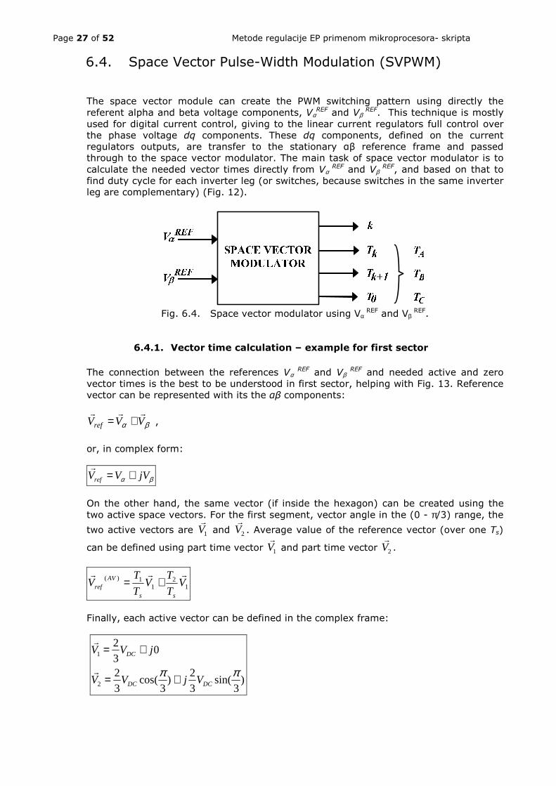
6.4. Space Vector Pulse-Width Modulation (SVPWM)

The space vector module can create the PWM switching pattern using directly the referent alpha and beta voltage components, Vα

REF and Vβ REF. This technique is mostly

used for digital current control, giving to the linear current regulators full control over the phase voltage dq components. These dq components, defined on the current regulators outputs, are transfer to the stationary αβ reference frame and passed through to the space vector modulator. The main task of space vector modulator is to calculate the needed vector times directly from Vα

REF and Vβ REF, and based on that to

find duty cycle for each inverter leg (or switches, because switches in the same inverter leg are complementary) (Fig. 12).

Fig. 6.4. Space vector modulator using Vα

REF and Vβ REF.

6.4.1. Vector time calculation – example for first sector

The connection between the references Vα REF and Vβ

REF and needed active and zero vector times is the best to be understood in first sector, helping with Fig. 13. Reference vector can be represented with its the αβ components:

βα VVVref

rrr+= ,

or, in complex form:

βα jVVVref +=r

On the other hand, the same vector (if inside the hexagon) can be created using the two active space vectors. For the first segment, vector angle in the (0 - π/3) range, the two active vectors are 1V

r and 2V

r. Average value of the reference vector (over one Ts)

can be defined using part time vector 1Vr and part time vector 2V

r.

12

11)( V

T

TV

T

TV

ss

AVref

rrr+=

Finally, each active vector can be defined in the complex frame:

)3

sin(3

2)

3cos(

3

2

03

2

2

1

ππDCDC

DC

VjVV

jVV

+=

+=

r

r


V

VT

TV 22

T

TV 11

2V

1V

REFV

60

30

2V

1V

REFV

3060

)3

cos(32

DCV DCV32

)3

sin(32

DCV

a) Reference vector generation b) active vectors in complex form

Fig .6.5. Reference vector in the first sector. Using all three above equations we can get:

( )

+

+=+

+=+

221

1211

2

3

3

2

2

1

3

2T

VjTT

VVjTVT

VTVTjVVT

DCDCss

s

βα

βα

rr

Splitting the equation on real and imaginary part we get:

sDC

sDC

ssDC

T

TV

T

TVV

T

T

T

TVV

22

21

33

23

32

21

32

==

+=

β

α

and:

+=

=

DCss

DC

DCs

V

VTTT

V

V

V

VTT

βα

β

321

23

3

1

2

Finally, the needed vector on-times are:

( )

DCs

DC

s

V

VTT

VVV

TT

β

βα

3

323

2

1

=

−=

In the case that T1 and T2 are defined as one half of PWM on–times (because of the double update mode of PWM peripheral unit of most µC):


( )

DC

s

DC

s

V

VTT

VVV

TT

β

βα

23

2

1

2

32/3

2

1

=

−=

6.4.2. Vector time calculation - all sectors

In this section, the generic relation between the Vα

REF and Vβ REF and needed space

vector times is derived and an equation that is valid for all the sectors is given. It is presumed that a motor is in the star connection and that Vα and Vβ voltages are referenced to the motor phases. Splitting vector equations into its real and imaginary

part (using βα jVVVref +=r

and 3/)1(

32 π−= kj

dck eVVr

), it follows that:

+

−

−=

+1

)3

sin(

)3

cos(

)3

)1sin((

)3

)1cos((

32

2 kkDCs T

k

kT

k

kV

TV

V

π

π

π

π

β

α

Tk and Tk+1 are defined as one half of vector on–times. Solving the system of equations we can get (if k=1, the same as equation for first sector):

( )

10

1

2

)3

)1cos((

)3

cos(

)3

)1sin((

)3

sin(2/3

+

+

−−=

−

−

−−=

kks

DC

s

k

k

TTT

T

V

V

k

k

k

k

V

T

T

T

β

α

π

π

π

π

k=1..6

Table with the predefined sine/cosine values for each sector can be written in 1.15

format, using 866.02/3 = , which is helpful for the implementation.

sector

(k) )

3sin(

πk )

3cos(

πk− )

3)1sin((π−− k )

3)1cos((π−k

1 0.866=28377 -0.5=-16383 0 =0 1= 32767

2 0.866=28377 0.5=16383 -0.866=-28377 0.5=16383

3 0 1= 32767 -0.866=-28377 -0.5=-16383

4 -0.866=-28377 0.5=16383 0 -1= -32767

5 -0.866=-28377 -0.5=-16383 0.866=28377 -0.5=-16383

6 0 -1= -32767 0.866=28377 0.5=16383

Table 1. Table containing all needed pre-calculated trigonometrically results.


6.5. Software implementation notes for SVPWM Firstly, the sector number must be found from reference voltages Vα

REF and Vβ REF, by

using scheme illustrated in Fig. 14.

Fig. 6.6. Sector determination using the references Vα

REF and Vβ REF.

If detected sector is k, the active vectors Vk and Vk+1 will be used. Next, the space vector times must be calculated. In order to have minimum number of online calculations, the following formula is used:

( )

10

1

2

)3

)1cos((3

)3

cos(3

)3

)1sin((3

)3

sin(32/

+

+

−−=

−

−

−−=

kks

DC

s

k

k

TTT

T

V

V

k

k

k

k

V

T

T

T

β

α

π

π

π

π

k=1,…,6

In that case, the predefined trigonometric results are numbers are in ±2 range, and 2.14 format must be used.

sector

(k) )

3sin(

πk )

3cos(

πk− )

3)1sin((π−− k )

3)1cos((π−k

1 1.5=24575 -0.433=-14188 0 =0 0.866=28377

2 1.5=24575 0.433=14188 -1.5=-24575 0.433=14188

3 0 0.866=28377 -1.5=-24575 -0.433=-14188

4 -1.5=-24575 0.433=14188 0 -0.866=-28377

5 -1.5=-24575 -0.433=-14188 1.5=24575 -0.433=-14188

6 0 -0.866=-28377 1.5=24575 0.433=14188

Table 6.1. Table containing all needed trigonometrically results in 2.14 format. Next, the calculated vector times needs to be distributed to particular PWM channels. PWM channel times are generated depending of the current sector. Situation for the first sector is shown in Fig. 15, where it is obvious that duty cycle for channel A has the longest on–time, and the duty cycle for channel C has the shortest on-time. Connection between the two vector times and zero time with the PWM channels on time is given in the next set of equations. The equations are valid for first sector only, but it can be


generalized for all sector based on this. On times of the channels are exactly half of the total PWM channel on-time during the one PWM period.

SMALLT

T

MIDDLETT

T

BIGTTT

T

C

kB

kkA

==

=+=

=++=

+

+

2

2

2

0

10

10

For any sector situation it is similar. First, BIG, MIDDLE and SMALL time are calculated.

2

2

2

0

10

10

TSMALL

TT

MIDDLE

TTT

BIG

k

kk

=

+=

++=

+

+

And then distributed to the right channels based on the following table.

Sector number

Loading PWM values

SECTOR 1 TA= BIG , TB= MIDDLE , TC= ZERO SECTOR 2 TA= MIDDLE, TB= BIG, TC= ZERO SECTOR 3 TA= ZERO , TB= BIG, TC= MIDDLE SECTOR 4 TA= ZERO , TB= MIDDLE, TC= BIG SECTOR 5 TA= MIDDLE , TB= ZERO, TC= BIG SECTOR 6 TA= BIG , TB= ZERO, TC= MIDDLE

Table 6.2. PWM channels on–times distribution for all sectors.

Fig. 6.7. Vector times versus PWM channel times for sector 1.


7. Motor current regulators in dq reference frame Motor currents are controlled in dq reference frame, as dc variables in stacionary reference frame. Also, we usually have the motor phase parameters and we should always try to regulate motor phase currents and give motor phase voltage references to SVPWM.

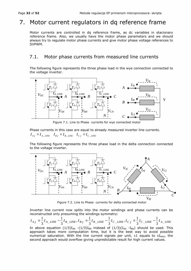
7.1. Motor phase currents from measured line currents The following figure represents the three phase load in the wye connection connected to the voltage inverter.

IA_LINE IB_LINE IC_LINE

T1

T2

T3

T4

T5

T6

A

B

C

YVDC

VAf

N

VAN VBN VCN

A B C

IAf

VBf

VCf

IBf

ICf

Figure 7.1. Line to Phase currents for wye connected motor

Phase currents in this case are equal to already measured inverter line currents.

LINECfCLINEBfBLINEAfA IIIIII ___ ===

The following figure represents the three phase load in the delta connection connected to the voltage inverter.


T1

T2

T3

T4

T5

T6

A

BC

VDC

N

VAN VBN VCN

A B C

VBf

VCf

IBf ICf

IAf VAf

Figure 7.2. Line to Phase currents for delta connected motor Inverter line current now splits into the motor windings and phase currents can be reconstructed only presuming the windings symmetry:

LINEALINECfCLINECLINEBfBLINEBLINEAfA IIIIIIIII ______ 3

1

3

1,

3

1

3

1,

3

1

3

1 −=−=−=

In above equation (1/3)IAN -(1/3)IBN instead of (1/3)(IAN -IBN) should be used. This approach takes more computation time, but it is the best way to avoid possible numerical saturation. With the line current signals per unit, ±1 equals to ±IMAX, the second approach would overflow giving unpredictable result for high current values.


7.2. Motor phase currents from abc to dq frame

Current vectors in αβ and dq coordinate system are always calculated using motor phase quantities, no matter what kind of winding connection is used. For abc αβ transformation (Clarke) coefficient 2/3 is used. As a consequence, αβ signals have the same amplitude as motor phase signals.

( )

( )

−=

+−=

CfBff

CfBfAff

III

IIII

2

3

3

2

2

1

3

2

β

α

For symmetrical system, the sum of all the voltages is zero, and final αβ transformation becomes:

( )CfBff

Aff

III

II

−=

=

3

3β

α

Ones the rotor flux vector position is known the phase current vectors can be transferred to the dq reference frame which rotates synchronously with the rotor flux vector. The current vector transformation to the dq coordinate system (Park transformation):

dqfdqfqf

dqfdqfdf

III

III

θθθθ

βα

βα

cossin

sincos

+−=

+=

These currents can be now fed to the current regulators which have dq voltage references on the outputs. Voltage references are than transferred from dq to αβ coordinate system using inversed transformation (Inverse Park)and fed to the space vector module.

dqREF

qfdqREF

dfREFf

dqREF

qfdqREF

dfREFf

VVV

VVV

θθ

θθ

β

α

cossin

sincos

+=

−=

7.3. Typical digital current control model

Ones transferred in dq coordinate system, current vector coordinates are DC signals in steady state. That allows regulation of current vector coordinates without the phase leg, typical for regulating the AC signals.

αβ

dq

PI reg

PI reg

dq

αβ

Space vector modulator

abc

αβ

θdq

IAf

IBf

ICf

Iαf

Iβf

Idf

Iqf

VdfREF

VqfREF

Vαf REF

Vβf REF

PWMA

PWMB

PWMC

IdfREF

IqfREF

Figure 7.3. Typical digital current control scheme used in vector control drive


7.4. Incremental dq current regulators with output limits

The motor phase currents are regulated in dq reference frame. There are two identical and independent PI regulators, each controlling one current vector coordinate. The only interaction between two regulators can occur when stator voltage vector saturates, imposing the limit for outputs of both current regulators. In order to deal with the saturation in more efficient way, the current regulators are designed in the incremental form. Discrete form of typical PI regulator:

errz

KerrKout i

p 11 −−+=

can be calculated using the following discrete equation:

)()()(

)()()(

kTerrKkTIkTout

kTerrKTkTIkTI

p

i

+=+−=

As one can see, first integral portion of regulator output is created. Than, new output is derived adding the proportional term. If output saturates, integral term can continue integrating the error, leading to the well know wind-up problem. Incremental PI form is derived from its discrete form:

errKerrzKzout ip +−=− −− )1()1( 11

Leading to the following discrete form:

[ ]errKzKoutzout ip +−+= −− )1( 11

In the case of incremental PI regulator, first incremental part is calculated, than output position is added:

[ ])()()(

)()()()(

kTInckToutkTout

kTerrKTkTerrkTerrKkTInc ip

+=

+−−=

Limiting the regulator output is now easy:

LOWLOW

HIGHHIGH

LIMITkToutLIMITkToutif

LIMITkToutLIMITkToutif

kTInckToutkTout

=<=>

+=

)()(

)()(

)()()(

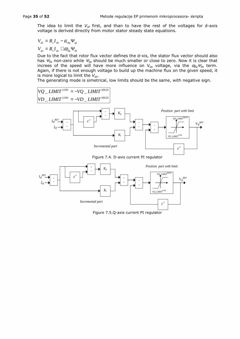
On the next two figures the models of incremental PI regulators used in d and q-axis are shown. Both regulators structures are identical. The only differences are the limits. For example, if the dq axis voltages represent the phase quantities of motor with delta connected windings the limits can be defined using the following: First, q voltage component should be limited to (for linear regime):

DCHIGH

q VLIMITVQV =≤ _

Than, d component should be limited in that way to limit the total vector amplitude:

22_ qDCHIGH

d VVLIMITVDV −=≤


The idea to limit the Vqf first, and than to have the rest of the voltages for d-axis voltage is derived directly from motor stator steady state equations.

dsdqqssqs

qsdqdssds

IRV

IRV

Ψ+=

Ψ−=

ωω

Due to the fact that rotor flux vector defines the d-xis, the stator flux vector should also has Ψds non-zero while Ψqs should be much smaller or close to zero. Now it is clear that increes of the speed will have more influence on Vqs voltage, via the ωdqΨds term. Again, if there is not enough voltage to build up the machine flux on the given speed, it is more logical to limit the Vqs. The generating mode is simetrical, low limits should be the same, with negative sign.

HIGHLOW

HIGHLOW

LIMITVDLIMITVD

LIMITVQLIMITVQ

__

__

−=

−=

Kp

z-1

+

-

Ki

+

-

IdfREF

Idf

+

+ +

+

VD_LIMITHIGH

VD_LIMITLOW

z-1

VdfREF

Incremental part

Position part with limit

Figure 7.4. D-axis current PI regulator

Kp

z-1

+

-

Ki

+

-

IqfREF

Iqf

+

+ +

+

VQ_LIMITHIGH

VQ_LIMITLOW

z-1

VqfREF

Incremental part

Position part with limit

Figure 7.5.Q-axis current PI regulator


7.5. Current regulators parameters evaluation There is several different procedures to determine current regulator parameters.

i

ip sT

sTK

+1 Kinv

s

s

s

K

τ+1

is

∑ is

REF

PI regulator inverter stator

vsREF Vs

bI

1

Figure 7.4. Current regulator parameters evaluation One gives:

inv

cbs

invs

cbsp K

IL

KK

IK

ωσωτ==

Gain of SV module is

DCinv VK =

Wanted current loop bandwidth: ωc= 2π100 rad/s Period of current control loop:

pwmTT =

Then, parameters of normalized PI regulator are:

siT τ=

inv

cbsApp K

ILKK

ωσ==

i

ApA

i T

KK =

For the digital automatic control system, with the period T, wanted PI integral action becomes:

TKK Aii =

In the case of following motor parameters, we can calculate needed proportional and integral gains for current controllers: - stator resistance: ][1,9 Ω=SR

- total leakage stator inductance: ][065,0 HLS =σ

It gives stator circuit time constant: ][1,7][0071,01,9

065,0mss

R

L

S

SS ==== στ

Defined base value for the current: ][8 AI b =


DC bus voltage is: ][340VVDC =

Wanted current loop bandwidth is: ]/[1002 sradc ⋅= πω

Switching PWM frequency is 16 kHz, so period of current loop is: ][5,621016

13

sT µ=⋅

=

Finally, based on this values needed PI parameters for current controllers (prepared for digital automatic control system) can be:

96096,0340

10028065,0 =⋅⋅⋅== πωσinv

cbsp K

ILK

00846,0105,620071,0

96096,0 6 =⋅== −TT

KK

i

pi

In per unit representation, in 1.15 format this values are:

27700846,032767

3148796096,032767

=⋅=

=⋅=

i

p

K

K

i.e. values that must be entered in software are: KP_GAIN = 0x7AFF (F1.15) KI_GAIN = 0x115 (F1.15) Another method (absolute value optimum) gives:

1071.0

2353.12

=

=

i

p

K

K


8. Discrete IFOC control

8.1. IFOC overview

It is already shown that if the slip frequency of drr

qsmk T

iL

ψω = is selected, the rotor flux

component in q-axis will be canceled , .0=+ qrqr

r dt

dT ψ

ψ

Result of that is alignment of rotor flux vector parallel with the d-axis of rotating frame. Amplitude of rotor flux vector can be controlled only using the d-axis component of stator current vector:

,dsmdrdr

r iLdt

dT =+ψψ

In the same time, the electrical torque can be controlled independently, using the q stator current component:

.2

3,

r

mTqsdrTel L

LpKiKT == ψ

Above given equations are the base for indirect field oriented control of rotor vector flux and independent control of electrical torque. Practical implementation of IFOC starts with estimation of rotor flux amplitude

dsr

mdr i

sT

L

+=

1ψ

Next, rotor slip frequency and slip angle are estimated:

dtT

iLk

drr

qsmk ∫== ωθ

ψω κ ˆˆ

ˆˆ

Finally, new dq frame angle is calculated using measured rotor angle and estimated slip angle.

krdq θθθ ˆˆˆ +=

Rotor position rθ can be directly measured from position sensor or estimated from rotor

speed information.

dtrr ∫= ωθ ˆˆ

8.2. Implementation of discrete IFOC equations IFOC can be implemented in microprocessor using discrete versions of above given

equations. Simple left Euler transformation can be used, T

zs

1−= .

8.2.1. Rotor flux amplitude estimation in 32-bit precision

Rotor flux amplitude estimation discrete model becomes:


( ) 1

1

1111

ˆ−

−

−+=

+−=

−+=

zT

T

T

T

ziL

zT

T

T

TiL

iz

T

TL

rr

dsm

rr

dsmds

r

mdrψ

Instead of rotor flux amplitude, for IFOC is easier to use filtered D axis current:

1

11

1'

11

)(ˆ)(

−

−−

−

−−

==z

T

T

ziT

T

L

zzi

r

dsr

m

drds

ψ

Discrete version of D axis filters equation:

)()(1)(*

'*

' TkTiT

TTkTi

T

TkTi ds

rds

rds −+−

−=

It is essential to use 32 bit precision for ids filter calculation. If there is no space or

calculation time, 16 bit version can be used, but parameters

−

*1

rT

T and

*rT

T must be

set to sum to precise 32768 (0x8000) value!. Not 32767! For example:

][097,0* sR

LT

r

rr ==

][5.6216000

11s

fTT

PWMPWM µ====

Next, using 16-bit arithmetic we have:

4*

104433,6][097,0

][5,62 −⋅==s

s

T

T

r

µ

In per unit representation, in 1.15 format, needed parameters has values:

15021104433,632768 4

15.1*

xT

T

Fr

==⋅⋅=

−

FEBxxxT

T

Fr

7015080000115.1

*=−=

−

Note: 8000015070 xxFEBx =+ !

8.2.2. Slip frequency and angle estimation in 32-bit precision Slip frequency can be calculated using:

)(

)(1)(

'* kTi

kTi

TkT

ds

qs

r

k =ω

But, in IFOC slip angle calculation is needed instead of slip frequency:


)(

)()()(

)(

)(1)(

)()()(

''* kTi

kTi

T

TTkTkT

kTi

kTi

TkT

kTTTkTkT

ds

qs

rkk

ds

qs

rk

kkk

+−=⇒

=

+−=θθ

ω

ωθθ

Additional correction of this equation is also needed, due to the fact that DSP is using relative angle range

RADIANSREL

RAD

REL

θπ

θππθ

θ 1

,

1,1=⇒

+−∈

+−∈

Therefore, relative slip angle can be calculated as:

)(

)(1)()(

' kTi

kTi

T

TTkTkT

ds

qs

rkk

+−=

πθθ

Angle must be kept and calculated in 32 bit precision, therefore used parameter is:

0x6B8792104433,61 31

4

31.1

=⋅⋅=

−

ππFrT

T

Note: Per unit division functions do not work if divider is bigger that numerous. The best way to do the division is to shift numerous for N places right before division call, making it smaller than divider. One must know what is the maximum possible Iq/Id ratio to decide number of places to be shifted. For example, the following 4 bits shift will allow Iq/Id ratio to be in the 0 – 16 range which is usually more than enough.

[ ]4

)(

4)(1)()(

'<<

>>

+−=

kTi

kTi

T

TTkTkT

ds

qs

rkk π

θθ

Possibility that Iq/Id can be higher than 16 must also be included in C-code. Temp16 = abs(Is_q_ref)>>MAX_IQ_ID_RATIO_LOG; Temp16= ( Temp16 > Is_d_filt)? 0x7FFF : Temp16/Is_d_filt;

For Iq/Id>16 the result will saturate but it will not result in negative slip frequency.

8.2.3. Rotor flux (dq frame) position estimation

Finally, new normalized rotor flux angle (±1 range) is estimated summing the estimated (calculated) slip position and measured (or estimated) rotor position.

)()()( kTkTkT krdq θθθ +=

)(kTkθ - It is shown how slip angle can be calculated

)(kTrθ - Rotor angle can be directly measured from position sensor (encoder or

resolver). Or, it can be integrated (summed) using the rotor speed information:

)()1()( kTTkTkT rrr ωθθ +−=


8.3. Simplified block diagram of IFOC control algorithm

Initialize S/W modules,

IFOC parameters PWM modul and interrupt

ADC modul QPEP modul

Start

Enable PWM interrupt

Background loop

PWM interrupt

Return

Theta_Rotor=ReadEncoder()

read ADC module (currents/DC bus voltage)

Execute for currents CLARKE/ and PARK transf. (with ThetaRFlux(kT-T))

Execute Current regulators with voltage limit.

Execute IFOC slip calculator Theta_Slip(kT)

ThetaRFlux(kT)= ThetaSlip+ThetaRotor

Execute Inverse Park for ref. voltages with ThetaRFlux(kT)

Execute SVGEN module

Update PWM registers

PWM intterupt

Figure 8.1. Basic IFOC algorithm

8.4. IFOC – quasi C-code implementation

We have to implement:

)()(1)(*

'*

' TkTiT

TTkTi

T

TkTi ds

rds

rds −+−

−= (all variables and coeff: 1.15 format)

)(

)(1)()(

' kTi

kTi

T

TTkTkT

ds

qs

rkk

+−=

πθθ ( kθ and

rT

T

π1

in 1.31, currents in 1.15)

)()()( kTkTkT krdq θθθ += ( ;15.1:)(kTdqθ :)(),( kTkT kr θθ 1.31)

C code to be implemented ..


9. Speed regulator Speed regulator is designed in incremental form. The speed regulator accepts the rotor speed measured via AC tachometer, and the speed reference from the speed ramp. The output of speed regulator is wanted electrical torque, or q-axis current reference. Having the real torque command on the output of speed regulator enhances the speed response and overall system dynamics and it is one of the advantages of IFOC control structure.

Kp

z-1

+

-

Ki

+

-

nRREF

nR +

+ +

+

IQ_LIMIT

-IQ_LIMIT

z-1

IqREF

Figure 8.1. Speed regulator block diagram

The parameters of the speed regulators are set during the experiment.

9.1. Speed regulator parameters calculation procedure

There is couple of procedures to determine current regulator parameters. To be defined ... 9.2. Maximum Q phase current calculation – current limit

In order to achieve the best dynamic it is necessary to calculate q phase current limit. To be defined ...

10. Field weakening – flux control In order to reach high speeds rotor flux weakening procedure must be defined. Simple feed-forward 1/w based method is not enough; some kind of flux controller based on dc voltage margin must be defined. To be defined ...


11. Induction motor parameters and data IFOC structure is based on motor parameter which must be initially defined and if needed , on –line estimated.

11.1. Initial Induction motor parameters and data 11.1.1. IM no load test

Rs, Lm, nominal D axis current can be established from motor non-load test.

To be defined ...

11.1.2. IM load test

Rr, Lr, Ls can be established from load test.

To be defined ...


12. Influence of Tr parameter error on IFOC

12.1. Dobro odabran paramater Tr*= Tr

IFOC control with sensor has only one important machine parameter, which is the rotor time constant. In order to determine exact rotor flux angle, Tr must be know.

U slučaju dobro podešene vrednosti parametra korišćene u kontroleru (Tr*=Tr)

procenjena vrednost položaja rotorskog fluksa je tačna i statorske struje se pravilno orijentišu u odnosu na rotorski fluks. Ako se u ovom slučaju zadrže konstantne vrednosti struja statora Ids0 i Iqs0, posle prelaznih procesa su ostvarene sledeće stacionarne vrednosti komponenti fluksa rotora:

00 dsmdr IL=Ψ ,

00 =qrΨ , (3.13.)

uz konstantnu učestanost klizanja:

0

00

1

ds

qs

rk I

I

T=ω . (3.14.)

12.2. Pogrešno odabran paramater Tr*≠ Tr

In real motor application the Tr is variable and depends upon flux saturation level and rotor temperature.

)(

)(

etemperaturR

levelsaturationLT

r

rr =

Therefore, in order to have correct IFOC alignment, the online estimation of rotor time constant must be provided. If not, when motor gets hot, speed will be correct but the motor losses will increase because the DQ frame is not aligned properly and the nominal flux is not produced.

Ako parametar Tr* korišćen u modelu rotorskog kola nije u skladu sa stvarnom

vremenskom konstantom rotora Tr, pri utisnutim Ids0 i Iqs0 više ne važe jednačine za ostvareni rotorski fluks date u (3.1). Izračunata učestanost klizanja

0

0*0

1

ds

qs

rk I

I

T=ω , (3.15.)

je različita od potrebne (3.2) i nove stacionarne vrednosti komponenti rotorskog fluksa se mogu dobiti na osnovu (3.4). Sistem jednačina stacionarne radne tačke za rotorsko kolo je dobijen na osnovu (2.24) eliminacijom komponenti prelaznog procesa:

000011

dsmr

qrkdrr

ILTT

=− ΨωΨ ,


000011

qsmr

drkqrr

ILTT

=+ ΨωΨ . (3.16.)

Rešavanjem (3.4) za stacionarne vrednosti komponenti vektora rotorskog fluksa se dobija:

20

0000

)(1 rk

qsrkdsmdr

T

ITIL

ωω

Ψ+

+= ,

20

0000

)(1 rk

dsrkqsmqr

T

ITIL

ωω

Ψ+

−= . (3.17.)

Jednačina (3.5) pokazuje da komponente rotorskog fluksa u pogonu sa pogrešnom Tr*

nisu jednake zadatim, i da zavise od obe komponente statorske struje. U izrazima (3.6) jasno su razdvojene zadata vrednost komponente vektora rotorskog fluksa i odstupanje nastalo usled nepodešene vrednosti parametra rotorskog kola:

020

0*00

)(1)1( qs

rk

rk

r

rmdsmdr I

T

T

T

TLIL

ωωΨ

+−+= ,

020

*0)(1

1)1(0 qs

rkm

r

rqr I

TL

T

T

ωΨ

+−+= .

0,0 0,5 1,0 1,5 2,0 0,80

0,85

0,90

0,95

1,00 Ψ dr0 / Ψ rn

I qs0 /I ds0

0,0 0,5 1,0 1,5 2,0 -0,10

-0,08

-0,06

-0,04

-0,02

0,00 Ψ qr0 / Ψ rn

I qs0 /I ds0

Sl. 3.2. Fluksa rotora u pogonu sa relativnom greškom Tr/Tr*= 1.25 pri promeni odnosa Iqs0 /Ids0 .

0,0 0,5 1,0 1,5 2,0 1,00

1,05

1,10

1,15

1,20

1,25 Ψ dr0 / Ψ rn

I qs0 /I ds0

0,0 0,5 1,0 1,5 2,0

0,00

0,05

0,10

0,15

0,20 Ψ qr0 / Ψ rn

I qs0 /I ds0


Sl. 3.2. Fluksa rotora u pogonu sa relativnom greškom Tr/Tr*= 0.75 pri promeni odnosa Iqs0 /Ids0 .

)(2

300000 dsqrqsdr

IIL

Lpm

r

mel ΨΨ −= , (3.18.)

gde je mel0 stacionarna vrednost momenta nepodešenog sistema pri konstantnim zadatim strujama statora Ids0 i Iqs0. Ako se komponente fluksa rotora uvrste, dobija se:

2

0

0*

2

0

0*

*

1

1

+

+

=

ds

qs

r

r

ds

qs

r

r

eloelo

I

I

T

T

I

I

T

T

mm (3.19.)

za stacionarnu vrednost ostvarenog momenta. Pritom, zadata vrednost glasi:

00

2*

2

3qsds

r

melo II

L

Lpm = . (3.20.)

0,0 0,5 1,0 1,5 2,0 0,7

0,8

0,9

1,0

1,1

1,2

1,3

m el 0

I

I qs

ds

0

0

T r / T r =1.25

1.15

1.05

1

0.95

0.85

0.75

*

* m el 0

Sl. 3.6. Odnos vrednosti razvijenog i zadatog momenta za različite odnose struja i Tr/Tr*


13. Signal data ranges for 12-bit ADC

Analogue to digital converter (ADC) unit provides a most important interface between the controller and the real system. Physical signals such are inverter currents, dc bus voltage and temperature are analogue signals. All of these are represented by measurement and conditioning electronic circuits as an electrical voltage between VREF

MIN and VREFMAX, which is directly proportional to the original signal. The purpose of

the ADC unit is to convert the analogue voltage in range of VREFMIN-VREF

MAX into the digital number, also of a specific range. Used measurement equipment and conditioning analog circuits must be designed in that way to carry the whole signal analogue and digital range without saturation and with minimal signal distortion. The relationship between the analogue input voltage VIN, the number of binary digits n used to represent the digital number and the digital number ADC_NUMBER that represents that analogue voltage is given by:

( ) MINREFn

MINREF

MAXREF

IN VVVNUMBERADC

V +−

−⋅=12

_

VREF

MAX and VREFMIN are reference voltages which are used to limit the analogue voltage

range. Any input voltage beyond these references will deliver a saturated digital number or if it pass maximum ratings according to the datasheet it can destroy the controller unit (µC). If the ADC has a 12-bit resolution, with VREF

MIN connected to the analog signal ground (VREF

MIN = 0) and VREFMAX connected to the DSP analogue power supply (VREF

MAX = 3,3 V), digital number is given by the following formula:

[ ][ ] 4095

3,3_ ⋅=

V

VVNUMBERADC IN

Although the ADC unit has 12-bits, which covers number range from 0 to 4095, the result is usually stored as 16-bit number in order to make the number in the fractional data range 1.15 which represents real number in range from -1.0 to 1.0 (with the resolution 2-15). So, the 12-bit digital result is shifted left by 3 (multiplied by 8) in 16-bit result register automatically via hardware (or for some µC by software) giving the result:

[ ][ ]

[ ][ ] 32760

3,384095

3,3_ ⋅=⋅⋅=

V

VV

V

VVRESULTADC ININ

That means the ADC result can be immediately used as positive 1.15 number, in the range 0-1.0 or more precisely, in the range of 0 – 32760/32767. In order to use the maximum available ADC signal range and to obtain maximum conversion resoultion, the input signal to be measured should be transformed via conditioning circuits to exactly 0 -3.3V range.

13.1. DC bus voltage measurement The DC bus voltage measurement is designed supposing a grid line voltage of 135 [V] on a 120 [V] line (grid codes allows +10% overvoltage, and by this we include +12,5% overvoltage), which gives maximum DC bus voltage of 2·√2·135 [V] = 381 [V], when voltage doubler is used. The similar number is valid for grid line voltage of 242 [V] (+5,2% overvoltage) on a 230 [V] line, without the voltage doubler. One must note that at least 400 [V] on the DC link must be measurable, without the saturation.


But, during the drive design one must consider possible fault situations. One of possible fault situations is possible uncontrolled regenerative DC braking. If one wants to be able to monitor the DC bus rise during this period, the DC bus maximum legible value must be increased. If we chose that maximum readable DC bus voltage by measurement circuits and ADC converter (3,3 V at the input) is 600,6 [V] (50% higher than in normal operation range) it gives voltage divider factor of 600,6/3,3 = 182. The selected voltage divider resistors should be a precise resistors with 1% tolerance, both R1 on the top and R2 on the bottom. Connection between the DC bus voltage and DC bus voltage variable in software is:

][R2R1

R1

3.3

1][

32767

32760

3.3

1.).( VVVVupV DCINDC ⋅

+⋅=⋅⋅=

DC bus voltage base is defined with the maximum readable DC bus voltage: [V] 6,600== MAXBASE VV

Finally, we get Vdc_bus variable as positive fractional number, in the 1.15 range (0-1.0):

base

DCDC V

VVupV

)(.).( =

For practical drive application, the off-line calibration constant should be added.

( )( ) 1_.).( <<⋅= RESULTADCKupV DCVDC KDCV constant should be in 2.14 format (±2), allowing numbers bigger and smaller than 1. That is why there is one shift to the left, transferring back the number is 1.15 format. (Note: F1.15*2.14 2.14 and 2.14<<1 1.15)

13.2. Inverter leg current measurement The current signal is bipolar, so the current must be readable by ADC unit while flowing in positive and negative directions. To accomplish that, current signal which can be either positive or negative must be transferred and adjusted in 0-3,3 [V] positive range. That means the current sense circuit must have offset adjustment, in order to set up output voltage biased in the middle of the ADC power supply:

][65.12

][3,3

2_ V

VVOFFSETCURRENT

MAXREF ===

The current sense circuit gain is adjusted to transfer the real current signals from ±IMAX range to the 3,3 [V] range. For 1 [kW] inverter application, the current shunt resister, and maximum readable current is chosen to be:

][60 Ω= mRSH (standard value)

][8 AI MAX ±=± This selection leads to the following current sense circuit gain:

4375,3810602

3,3

2_

3=

⋅⋅⋅=

⋅⋅= −

MAXSH

MAXREF

IR

VGAINCURRENT

Although the 1% precise resisters are used in building the amplifier with needed offset and gain, the off-line drive calibrations is usually needed for the best performance. Also, during the stand still, periodical offset reading and filtering is also recommended. Output current result can be expressed as:


[ ]MAX

REF

MAXREF

SHMAXREF

IN

V

VAIRGAINCURRENT

V

VNUMBERCURRENT

32760

2_32760_ ⋅

+⋅⋅=⋅=

Separating the offset and the real signal:

[ ]1638032760

__ +⋅⋅⋅=

MAXREF

SH

V

AIRGAINCURRENTNUMBERCURRENT

Offset is never exactly one half of the number range and it must be recalculated during the stand still stage. That is why the offset variable is used , ADC_current_offset. To make the best precision in filtering possible, the variable is kept in 32-bit.

[ ]offsetcurrentADC

V

AIRGAINCURRENTNUMBERCURRENT

MAXREF

SH __32760_

_ +⋅⋅⋅=

After the current sample is ready, the offset must be removed. Presuming that the offset is removed entirely, the variable now holds:

[ ] 16380_ ⋅⋅= AI

V

RGAINCURRENTCURRENT

MAXREF

SH

Setting up the IBASE value in the software to be:

][8 AII MAXBASE ==

we get:

[ ]SH

MAXREF

BASEBASE RGAINCURRENT

VI

I

AICURRENT

⋅⋅=⋅=

_2,16380

Clearly, this number is now in ±16380 range, which is not convenient for further signal processing. The best is to have all the voltage and current measured signals in 1.15 format, ±32767 range representing fractional numbers in ±1. So, in order to use the current sample in 1.15 format, and further to process it with maximum numerical precision for 16 bit variables, one extra left shift is needed (multiplication by 2). Finally,

[ ]163802.).( ⋅⋅=

BASEI

AIupCURRENT

To accomplish this, the new current sample is calculated using this equation.

( ) 1___.).( <<−= offsetcurrentADCNUMBERCURRENTupCURRENT

For practical drive application, the off-line calibration constant should be added. ( )( ) 2___.).( <<−⋅= offsetcurrentADCNUMBERCURRENTKupCURRENT C

KC constant is kept in 2.14 format (±2), which allows numbers bigger and smaller than 1. That is why second shift left is also needed, in total two shifts left.

14. Appendix- Motor phase voltage and currents The terminal quantities that are typically measured or estimated from the voltage inverter side are the line currents and phase to ground voltage. Line currents are measured using up to three current sensors which can be placed on different places: connected on inverter outputs, or inverters legs bellow the bottom IGBT or in the DC bus circuit. But, in each combination, the currents sensor is in the path of inverter line


current. On the other hand, the inverter output voltage is usually estimated using commanded PWM pattern, which is relatively to the DC bus ground. From the motor side, the winding (motor phase) voltage and current are required. The different links between the motor phase quantities with the terminal quantities from the inverter side are discussed in the chapter.

14.1. Motor phase windings connected in the wye connection The following figure represents the three phase load in the star connection connected to the voltage inverter.


T1

T2

T3

T4

T5

T6

A

B

C

YVDC

VAf

N

VAN VBN VCN

A B C

IAf

VBf

VCf

IBf

ICf

Figure 6.1.

Phase currents in this case are equal to already measured inverter line currents.

LINECfCLINEBfBLINEAfA IIIIII ___ ===

Phase voltages can be reconstructed using inverter line to ground voltages.

BNANCNfC

CNANBNfB

CNBNANfA

VVVV

VVVV

VVVV

3

1

3

1

3

23

1

3

1

3

23

1

3

1

3

2

−−=

−−=

−−=

In above equation (1/3)VBN -(1/3)VCN instead of (1/3)(VBN +VCN) should be used. This approach takes more computation time, but it is the best way to avoid possible numerical saturation which can be a problem for add/sub operations, especially if the voltages are higher than half of the VBASE.

14.2. Motor phase windings connected in the delta connection The following figure represents the three phase load in the delta connection connected to the voltage inverter.



T1

T2

T3

T4

T5

T6

A

BC

VDC

N

VAN VBN VCN

A B C

VBf

VCf

IBf ICf

IAf VAf

Figure 6.2.

Inverter line current now splits into the motor windings and phase currents can be reconstructed only presuming the windings symmetry:

LINEALINECfC

LINECLINEBfB

LINEBLINEAfA

III

III

III

__

__

__

3

1

3

13

1

3

13

1

3

1

−=

−=

−=

In above equation (1/3)IAN -(1/3)IBN instead of (1/3)(IAN -IBN) should be used. This approach takes more computation time, but it is the best way to avoid possible numerical saturation. With the line current signals per unit, ±1 equals to ±IMAX, the second approach would overflow giving unpredictable result for high current values. Phase voltages can be reconstructed using inverter line to ground voltages.

ANCNfC

CNBNfB

BNANfA

VVV

VVV

VVV

−=

−=

−=

14.3. Phase voltages and currents in αβ coordinate system Voltage and current vectors in αβ and dq coordinate system are always calculated using motor phase quantities, no matter what kind of winding connection is used. For abc αβ transformation (Clarke) coefficient 2/3 is used. As a consequence, αβ signals have the same amplitude as motor phase signals.

( )

( )

−=

+−=

CfBff

CfBfAff

VVV

VVVV

2

3

3

2

2

1

3

2

β

α

For symmetrical system, the sum of all the voltages is zero, and final αβ transformation becomes:

( )CfBff

Aff

VVV

VV

−=

=

3

3β

α

The same is valid for phase currents and final equation to be used is:


( )CfBff

Aff

III

II

−=

=

3

3β

α

14.4. Phase voltages and currents in dq coordinate system Ones the rotor flux vector position is known the phase voltage and current vectors can be transferred to the dq reference frame which rotates synchronously with the rotor flux vector. The current vector transformation to the dq coordinate system (Park transformation):

dqfdqfqf

dqfdqfdf

III

III

θθθθ

βα

βα

cossin

sincos

+−=

+=

Voltages vector can also be transformed in dq coordinates system but this is typically not used in IFOC.

dqfdqfqf

dqfdqfdf

VVV

VVV

θθθθ

βα

βα

cossin

sincos

+−=

+=

Usually, only phase currents are transferred from αβ to dq coordinate system. These currents are than fed to the current regulators which have dq voltage references on the outputs. Voltage references are than transferred from dq to αβ coordinate system using inversed transformation (Inverse Park)and fed to the space vector module.

dqREF

qfdqREF

dfREFf

dqREF

qfdqREF

dfREFf

VVV

VVV

θθ

θθ

β

α

cossin

sincos

+=

−=

metode regulacije ep primenom mikroprocesora - skripta

Documents

simplified block diagram

tr parameter error

indirektna vektroska kontrola

tr jtr 1

rotating reference frame

ifoc praktina implementacija

ifoc teorijske osnove

rotora asinhrone maine