metrology and sensing - uni-jena.demetrology+and... · universal coordinate measuring machine (cmm)...
TRANSCRIPT
www.iap.uni-jena.de
Metrology and Sensing
Lecture 8: Geometrical methods
2017-12-07
Herbert Gross
Winter term 2017
2
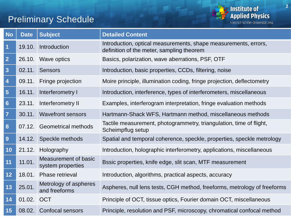
Preliminary Schedule
No Date Subject Detailed Content
1 19.10. Introduction Introduction, optical measurements, shape measurements, errors,
definition of the meter, sampling theorem
2 26.10. Wave optics Basics, polarization, wave aberrations, PSF, OTF
3 02.11. Sensors Introduction, basic properties, CCDs, filtering, noise
4 09.11. Fringe projection Moire principle, illumination coding, fringe projection, deflectometry
5 16.11. Interferometry I Introduction, interference, types of interferometers, miscellaneous
6 23.11. Interferometry II Examples, interferogram interpretation, fringe evaluation methods
7 30.11. Wavefront sensors Hartmann-Shack WFS, Hartmann method, miscellaneous methods
8 07.12. Geometrical methods Tactile measurement, photogrammetry, triangulation, time of flight,
Scheimpflug setup
9 14.12. Speckle methods Spatial and temporal coherence, speckle, properties, speckle metrology
10 21.12. Holography Introduction, holographic interferometry, applications, miscellaneous
11 11.01. Measurement of basic
system properties Bssic properties, knife edge, slit scan, MTF measurement
12 18.01. Phase retrieval Introduction, algorithms, practical aspects, accuracy
13 25.01. Metrology of aspheres
and freeforms Aspheres, null lens tests, CGH method, freeforms, metrology of freeforms
14 01.02. OCT Principle of OCT, tissue optics, Fourier domain OCT, miscellaneous
15 08.02. Confocal sensors Principle, resolution and PSF, microscopy, chromatical confocal method
3
Content
Tactile measurement
Triangulation
Scheimpflug setup
Stereo-Photogrammetry
Time of flight
4
Overview: Resolution vs Working distance
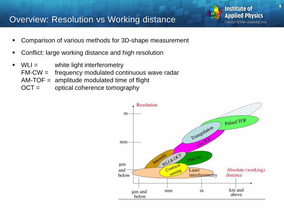
Comparison of various methods for 3D-shape measurement
Conflict: large working distance and high resolution
WLI = white light interferometry
FM-CW = frequency modulated continuous wave radar
AM-TOF = amplitude modulated time of flight
OCT = optical coherence tomography
5
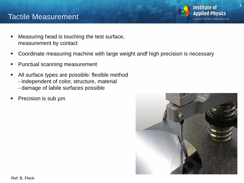
Tactile Measurement
Measuring head is touching the test surface,
measurement by contact
Coordinate measuring machine with large weight andf high precision is necessary
Punctual scanning measurement
All surface types are possible: flexible method
- independent of color, structure, material
- damage of labile surfaces possible
Precision is sub µm
Ref: B. Fleck
6
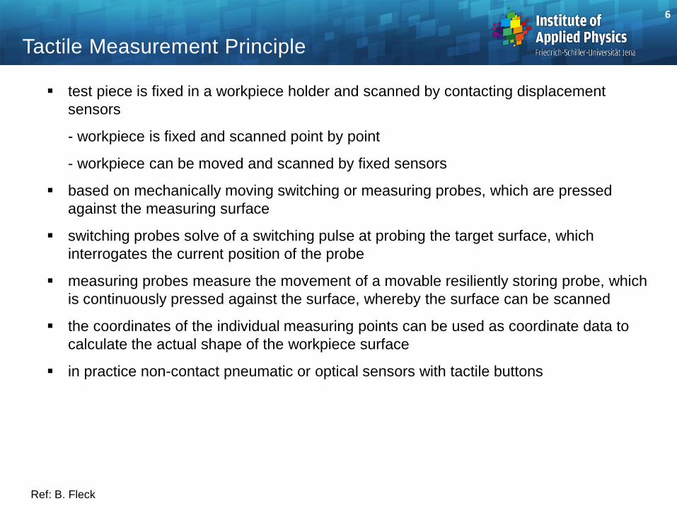
Tactile Measurement Principle
Ref: B. Fleck
test piece is fixed in a workpiece holder and scanned by contacting displacement
sensors
- workpiece is fixed and scanned point by point
- workpiece can be moved and scanned by fixed sensors
based on mechanically moving switching or measuring probes, which are pressed
against the measuring surface
switching probes solve of a switching pulse at probing the target surface, which
interrogates the current position of the probe
measuring probes measure the movement of a movable resiliently storing probe, which
is continuously pressed against the surface, whereby the surface can be scanned
the coordinates of the individual measuring points can be used as coordinate data to
calculate the actual shape of the workpiece surface
in practice non-contact pneumatic or optical sensors with tactile buttons
7
Tactile Measurement
Ref: B. Fleck
Applications:
- used for geometric control of coarse or fine shape deviations of workpieces:
- quality control by sampling or complete testing
- statistical process control
- determination of geometric models
Used in the measuring room or in the manufacturing environment
Suitable for the measurement of sufficiently solid surfaces, independent of color,
material and lighting conditions
Systems for coordinate metrology, form metrology and surface and contour
measurement technology are basically universally
Tested products for example:
metal parts, gears or complete vehicle bodies
8
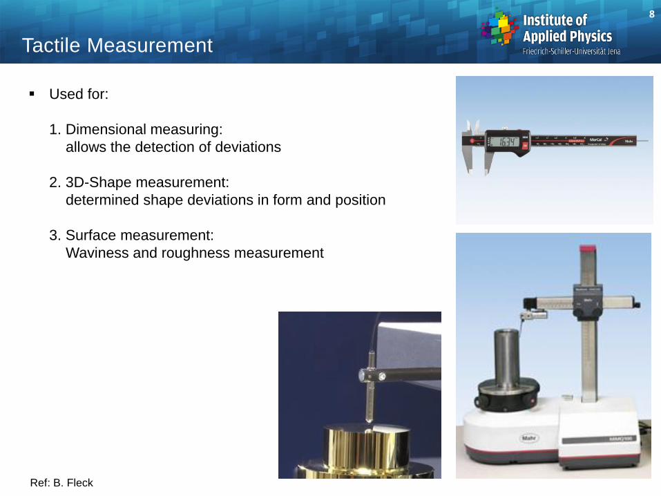
Tactile Measurement
Used for:
1. Dimensional measuring:
allows the detection of deviations
2. 3D-Shape measurement:
determined shape deviations in form and position
3. Surface measurement:
Waviness and roughness measurement
Ref: B. Fleck
9
Tactile Measurement
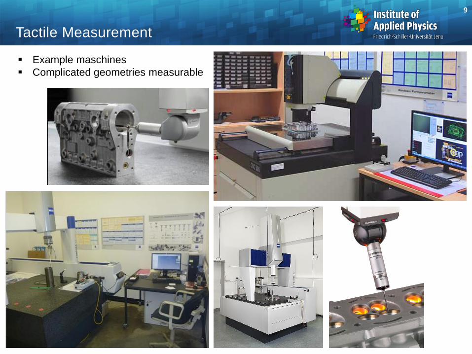
Example maschines
Complicated geometries measurable
Tactile Measurement
Ref: H. Hage / R.Börret
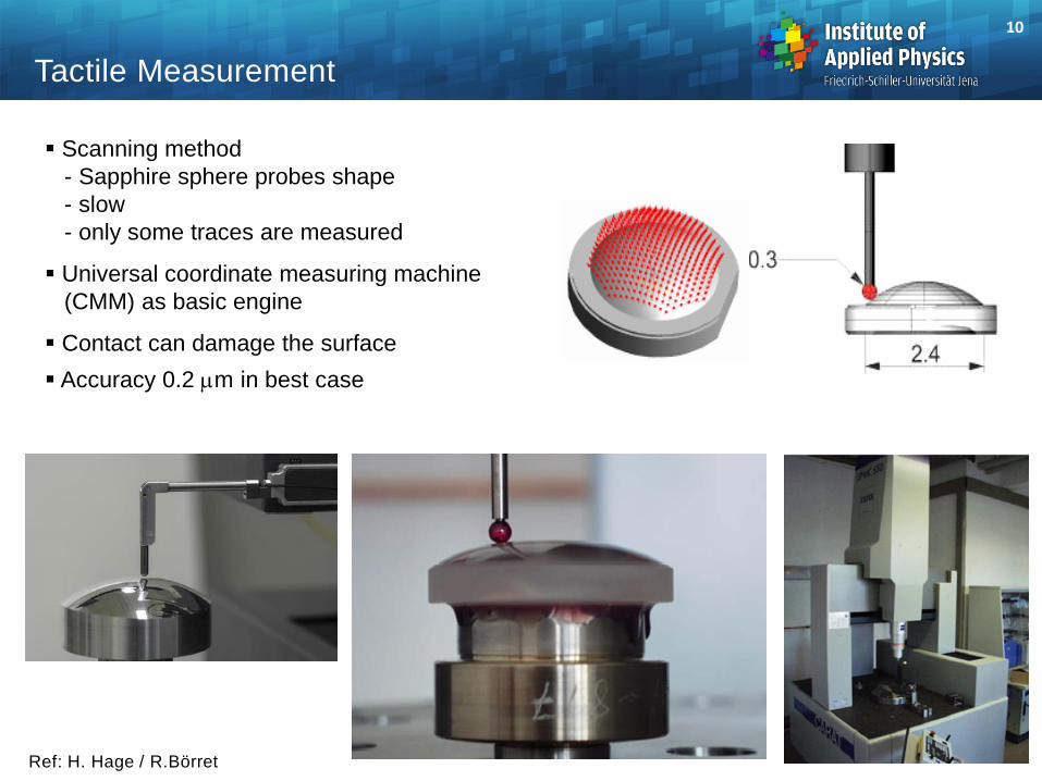
Scanning method
- Sapphire sphere probes shape
- slow
- only some traces are measured
Universal coordinate measuring machine
(CMM) as basic engine
Contact can damage the surface
Accuracy 0.2 mm in best case
10
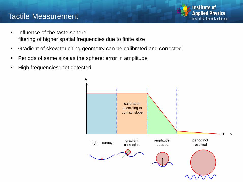
Influence of the taste sphere:
filtering of higher spatial frequencies due to finite size
Gradient of skew touching geometry can be calibrated and corrected
Periods of same size as the sphere: error in amplitude
High frequencies: not detected
Tactile Measurement
A
high accuracy
v
gradient
correction
amplitude
reduced
period not
resolved
calibration
according to
contact slope
12
Tactile Measurement
Ref: B. Fleck
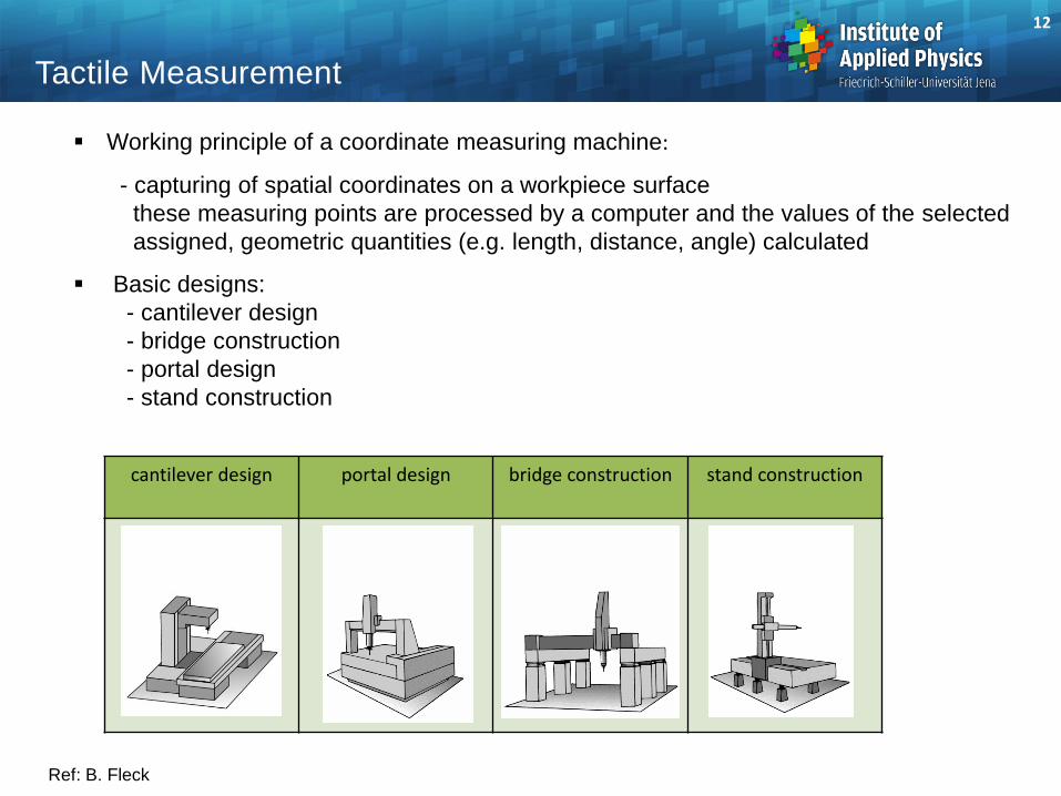
Working principle of a coordinate measuring machine:
- capturing of spatial coordinates on a workpiece surface
these measuring points are processed by a computer and the values of the selected
assigned, geometric quantities (e.g. length, distance, angle) calculated
Basic designs:
- cantilever design
- bridge construction
- portal design
- stand construction
cantilever design portal design
bridge construction stand construction
13
Coordinate Measurement Machine
Ref: B. Fleck
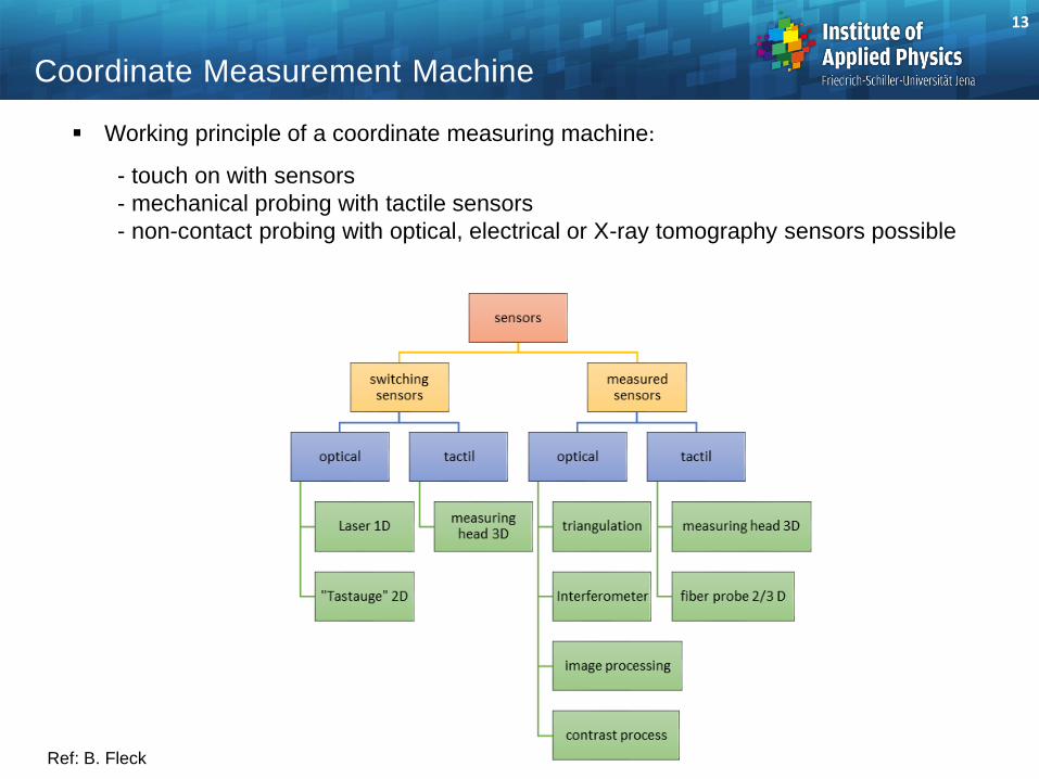
Working principle of a coordinate measuring machine:
- touch on with sensors
- mechanical probing with tactile sensors
- non-contact probing with optical, electrical or X-ray tomography sensors possible
14
Triangulation
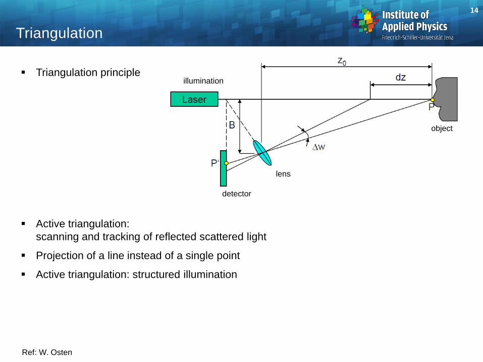
Triangulation principle
Active triangulation:
scanning and tracking of reflected scattered light
Projection of a line instead of a single point
Active triangulation: structured illumination
Ref: W. Osten
object
detector
lens
illumination
15
Triangulation
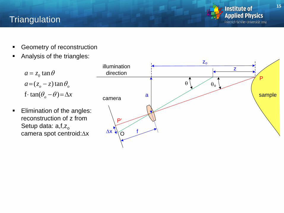
Geometry of reconstruction
Analysis of the triangles:
Elimination of the angles:
reconstruction of z from
Setup data: a,f,zo
camera spot centroid:Dx
camera
zo
z
a
P
P’
sample
illumination
direction
ODx
q qo
f
0 tan
( ) tan
f tan( )
o o
o
a z
a z z
x
q
q
q q
D
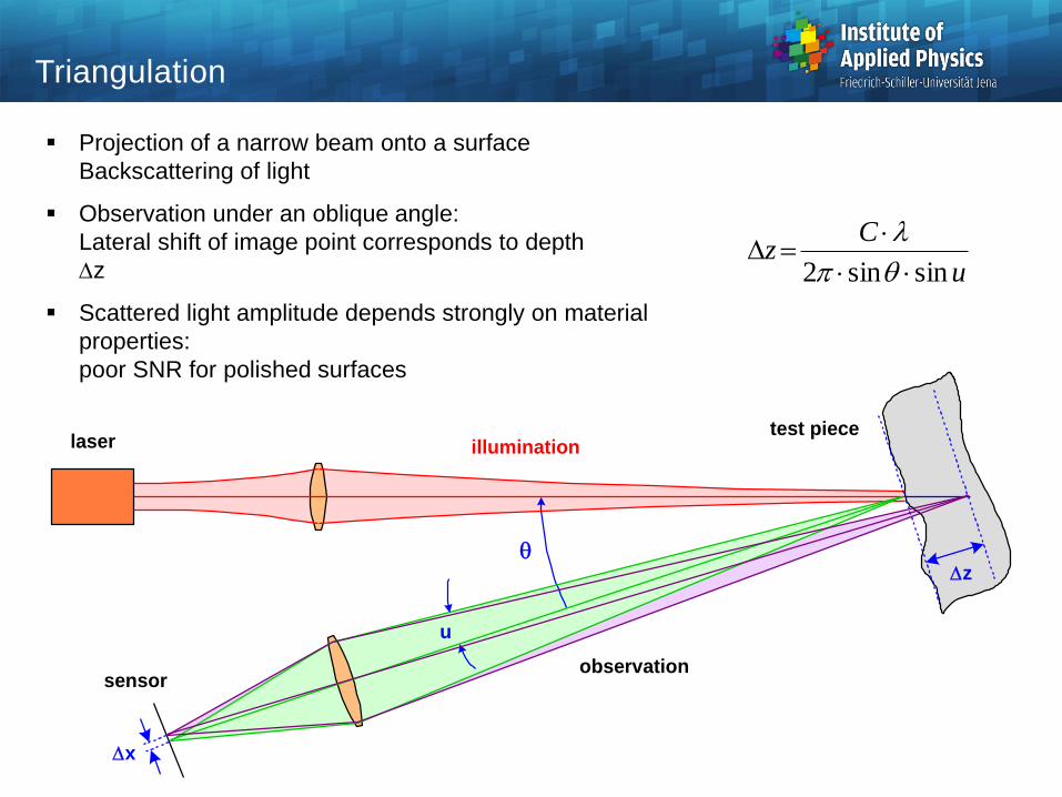
Projection of a narrow beam onto a surface
Backscattering of light
Observation under an oblique angle:
Lateral shift of image point corresponds to depth
Dz
Scattered light amplitude depends strongly on material
properties:
poor SNR for polished surfaces
u
Cz
sinsin2
D
q
Triangulation
q
test piece
u
sensor
illumination
observation
Dx
Dz
laser
17
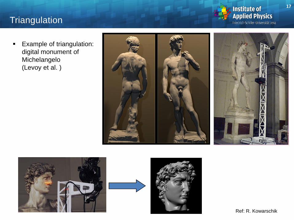
Triangulation
Example of triangulation:
digital monument of
Michelangelo
(Levoy et al. )
Ref: R. Kowarschik
18
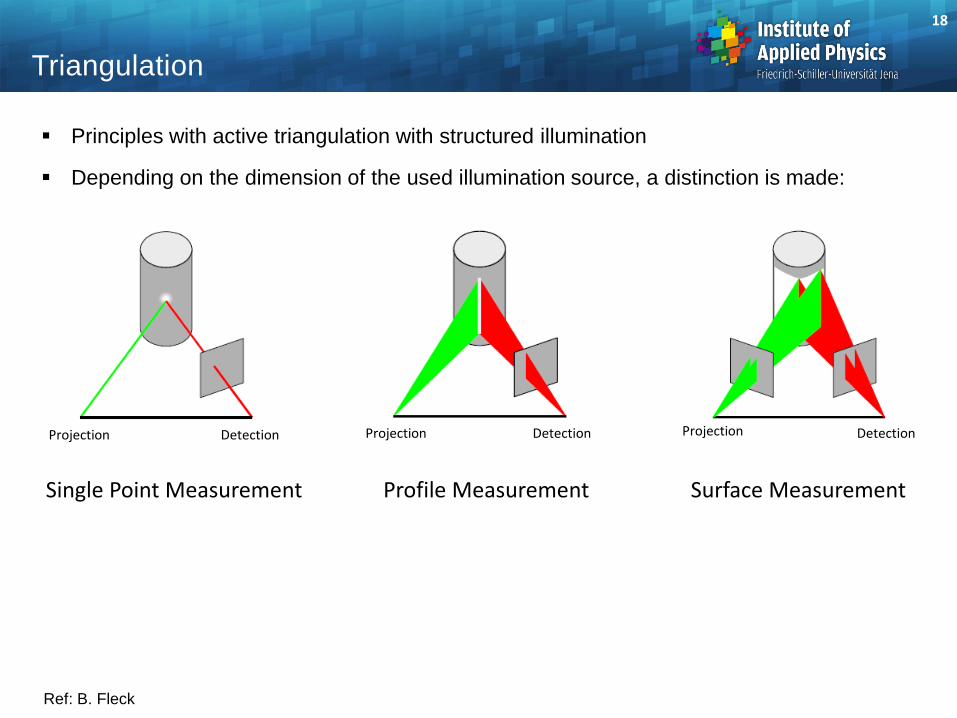
Triangulation
Ref: B. Fleck
Single Point Measurement Profile Measurement Surface Measurement
Projection Projection Projection Detection Detection Detection
Principles with active triangulation with structured illumination
Depending on the dimension of the used illumination source, a distinction is made:
19
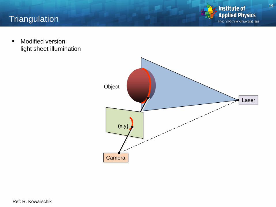
Triangulation
Modified version:
light sheet illumination
Ref: R. Kowarschik
Camera
Object
Laser
(x,y)
20
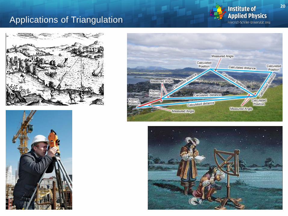
Applications of Triangulation
21
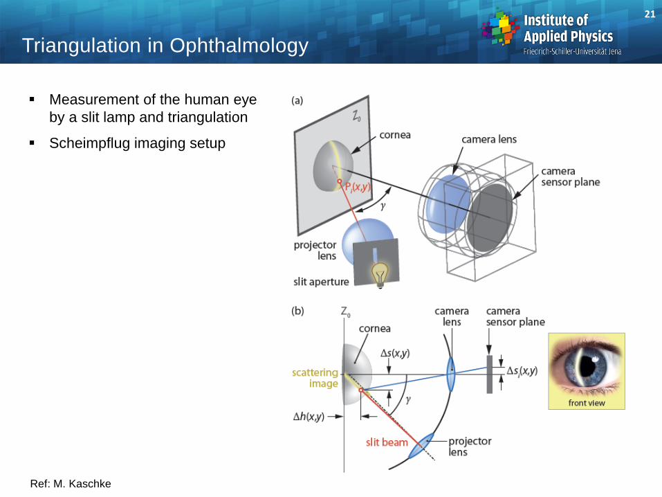
Triangulation in Ophthalmology
Measurement of the human eye
by a slit lamp and triangulation
Scheimpflug imaging setup
Ref: M. Kaschke
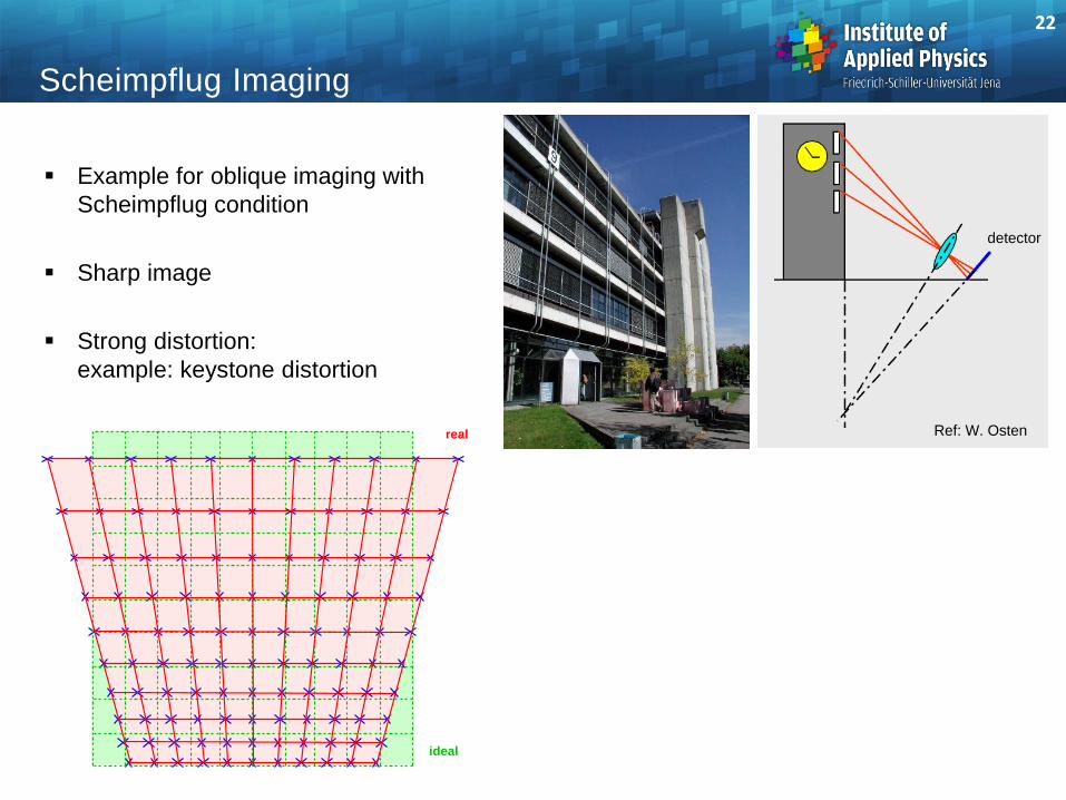
Scheimpflug Imaging
Example for oblique imaging with
Scheimpflug condition
Sharp image
Strong distortion:
example: keystone distortion
Ref: W. Osten
detector
22
ideal
real

General :
1. Image plane is tilted
2. Magnification is anamorphic
Example :
Scheimpflug-Imaging
Scheimpflug System
object plane
lens
image plane
q q'
s
s'
'sin
sin2
q
q oy mm
q
q
tan
'tan'
s
smm ox
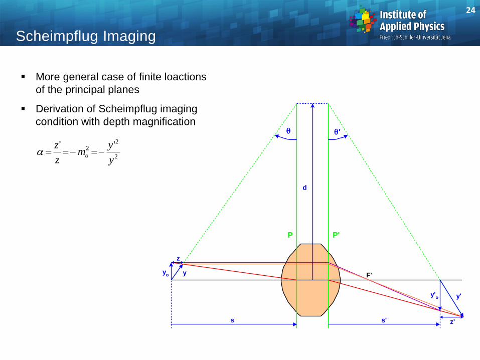
More general case of finite loactions of the principal planes
Derivation of Scheimpflug imaging
condition with depth magnification
Scheimpflug Imaging
yo
z
z'
P P'
F'
s's
q q'
d
y'o y'
y
2
22 ''
y
ym
z
zo
24
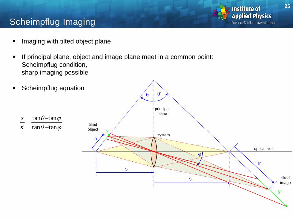
Imaging with tilted object plane
If principal plane, object and image plane meet in a common point:
Scheimpflug condition,
sharp imaging possible
Scheimpflug equation
q
q
tan'tan
tantan
'
s
s
Scheimpflug Imaging
q q'
y
s
s'
h
y'
h'
tilted
object
tilted
image
system
optical axis
principal
plane
25
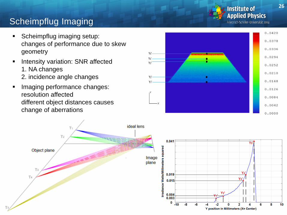
Scheimpflug imaging setup:
changes of performance due to skew
geometry
Intensity variation: SNR affected
1. NA changes
2. incidence angle changes
Imaging performance changes:
resolution affected
different object distances causes
change of aberrations
Scheimpflug Imaging
26
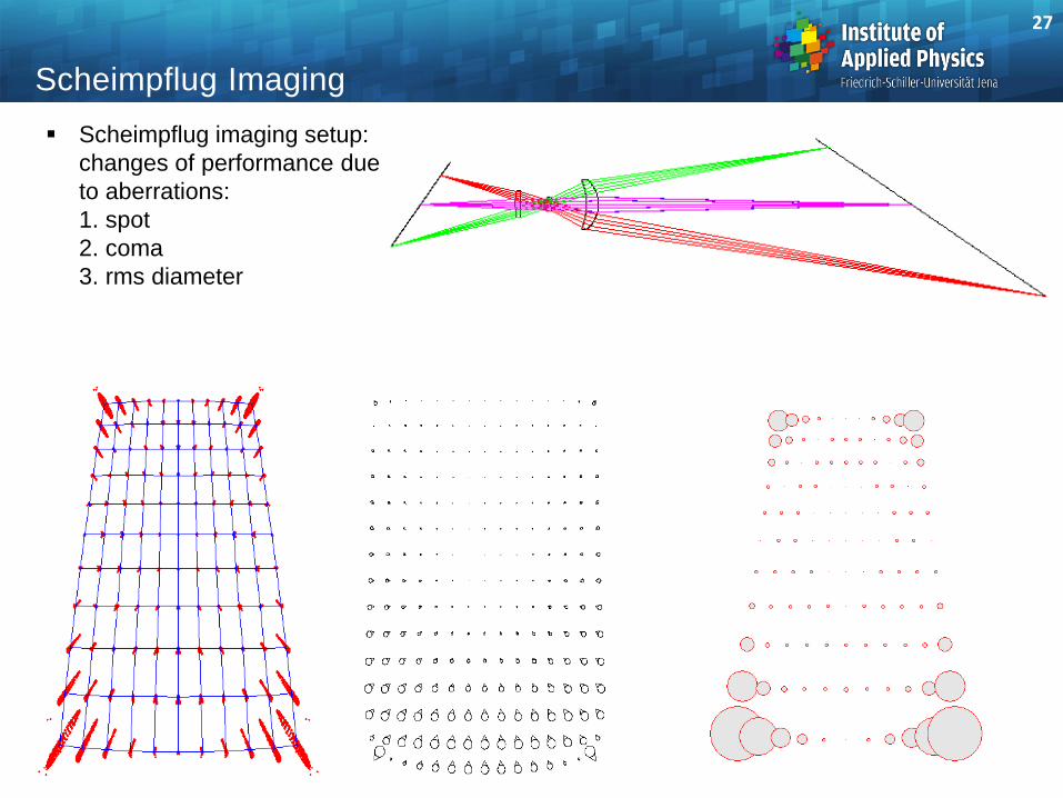
Scheimpflug imaging setup:
changes of performance due
to aberrations:
1. spot
2. coma
3. rms diameter
Scheimpflug Imaging
27
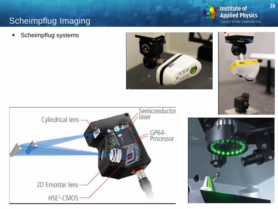
Scheimpflug systems
Scheimpflug Imaging
28
29
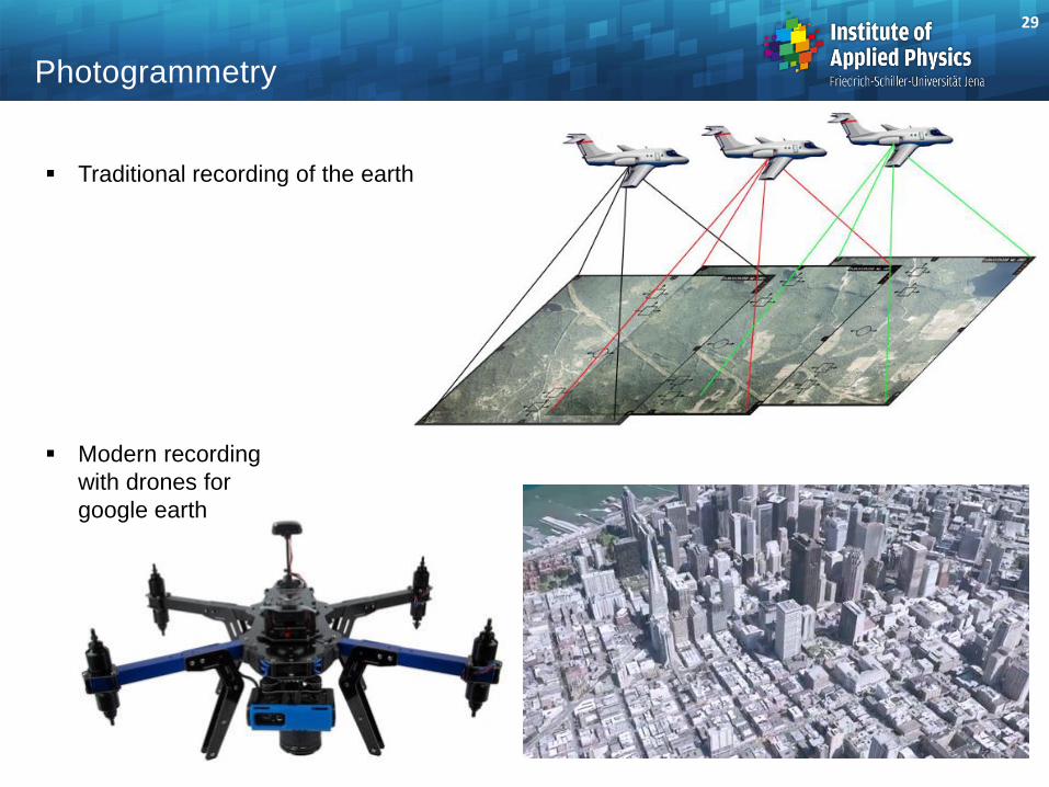
Photogrammetry
Traditional recording of the earth
Modern recording
with drones for
google earth
30
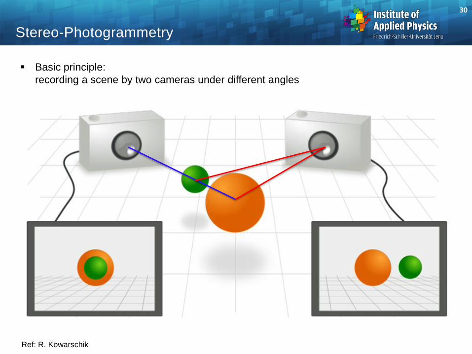
Stereo-Photogrammetry
Basic principle:
recording a scene by two cameras under different angles
Ref: R. Kowarschik
31
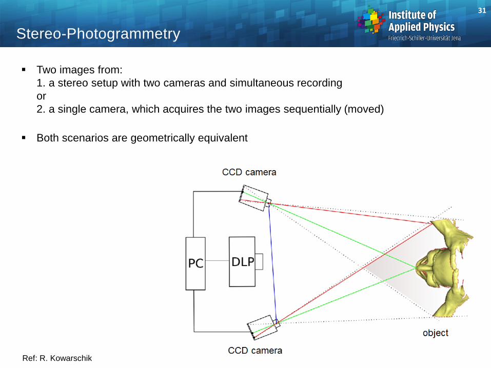
Stereo-Photogrammetry
Two images from:
1. a stereo setup with two cameras and simultaneous recording
or
2. a single camera, which acquires the two images sequentially (moved)
Both scenarios are geometrically equivalent
Ref: R. Kowarschik
32
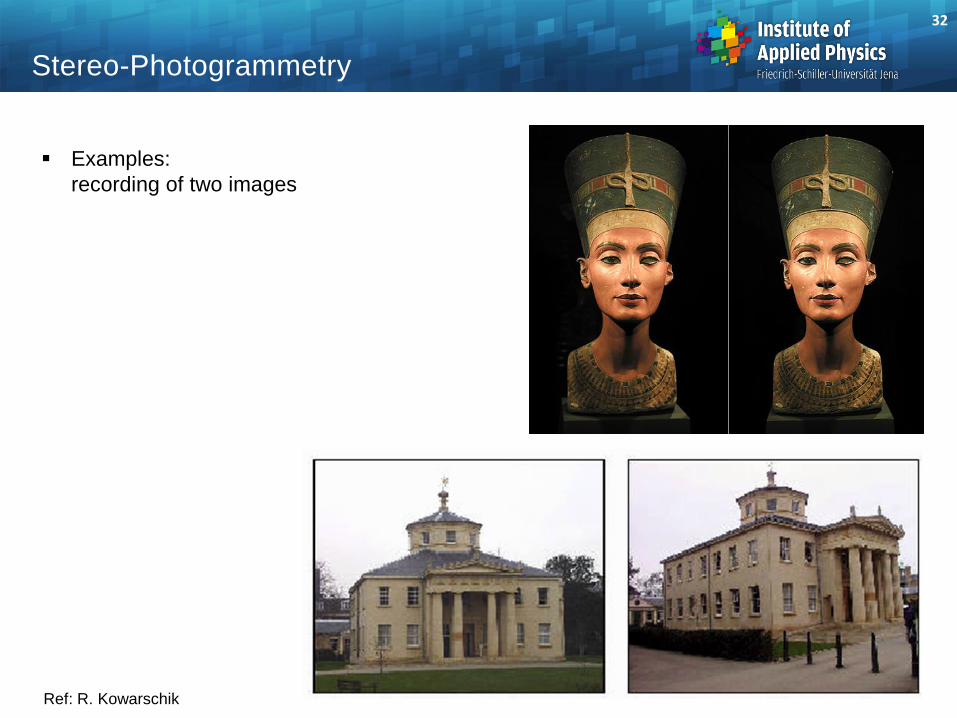
Stereo-Photogrammetry
Examples:
recording of two images
Ref: R. Kowarschik
33
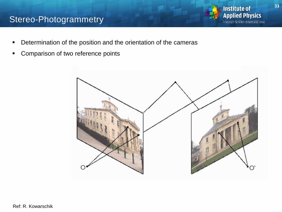
Stereo-Photogrammetry
Determination of the position and the orientation of the cameras
Comparison of two reference points
Ref: R. Kowarschik
34
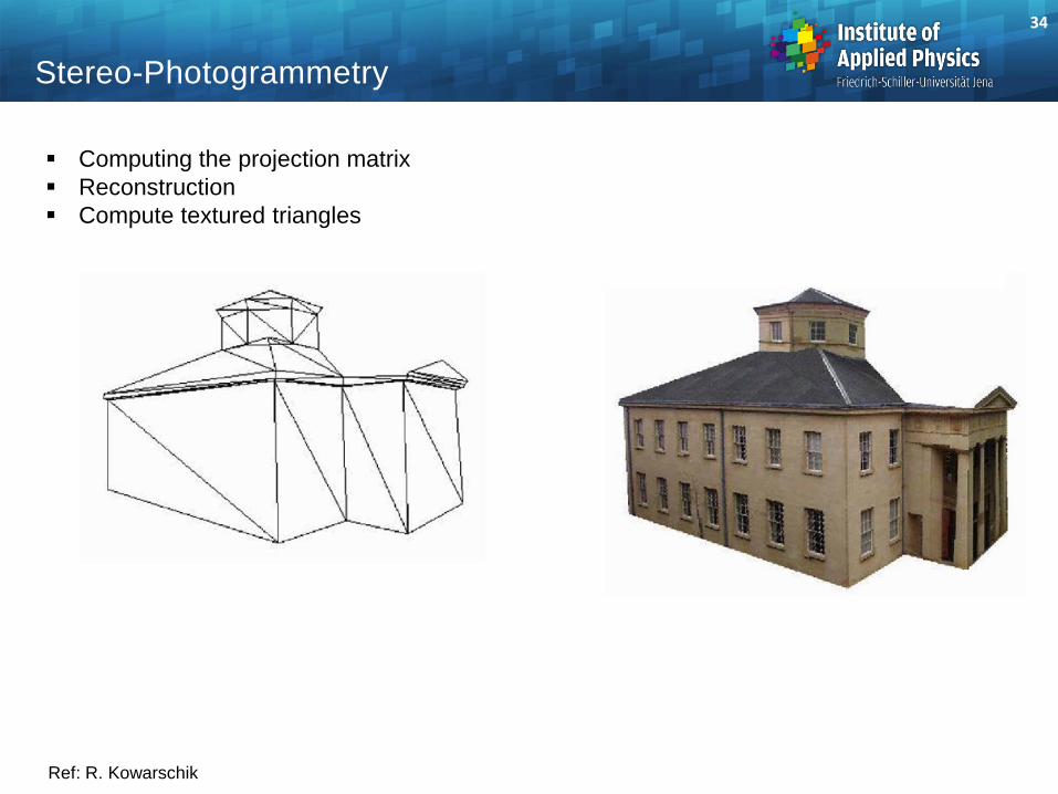
Stereo-Photogrammetry
Computing the projection matrix
Reconstruction
Compute textured triangles
Ref: R. Kowarschik
35
Stereo-Photogrammetry
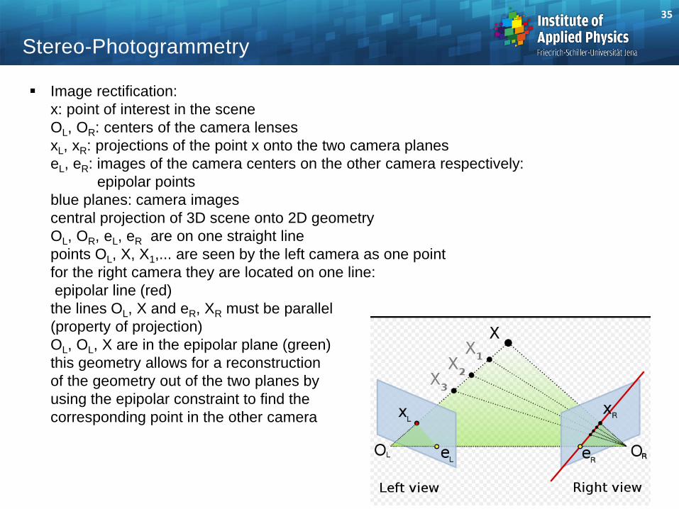
Image rectification:
x: point of interest in the scene
OL, OR: centers of the camera lenses
xL, xR: projections of the point x onto the two camera planes
eL, eR: images of the camera centers on the other camera respectively:
epipolar points
blue planes: camera images
central projection of 3D scene onto 2D geometry
OL, OR, eL, eR are on one straight line
points OL, X, X1,... are seen by the left camera as one point
for the right camera they are located on one line:
epipolar line (red)
the lines OL, X and eR, XR must be parallel
(property of projection)
OL, OL, X are in the epipolar plane (green)
this geometry allows for a reconstruction
of the geometry out of the two planes by
using the epipolar constraint to find the
corresponding point in the other camera
36
Stereo-Photogrammetry
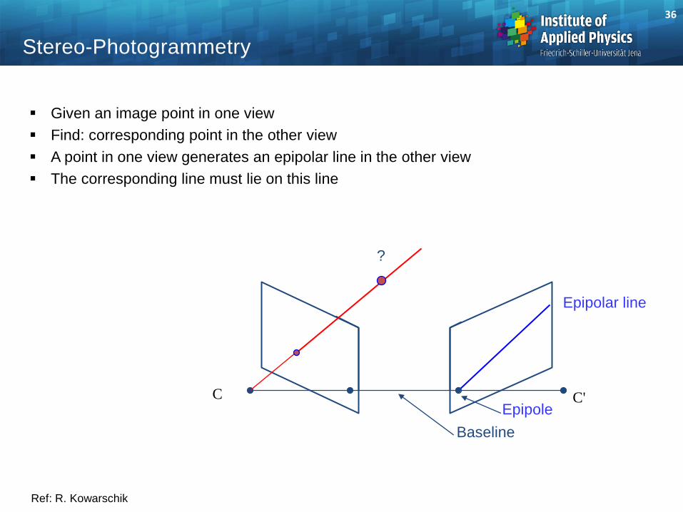
Given an image point in one view
Find: corresponding point in the other view
A point in one view generates an epipolar line in the other view
The corresponding line must lie on this line
Ref: R. Kowarschik
Epipolar line
?
Baseline
Epipole C' C
37
Stereo-Photogrammetry
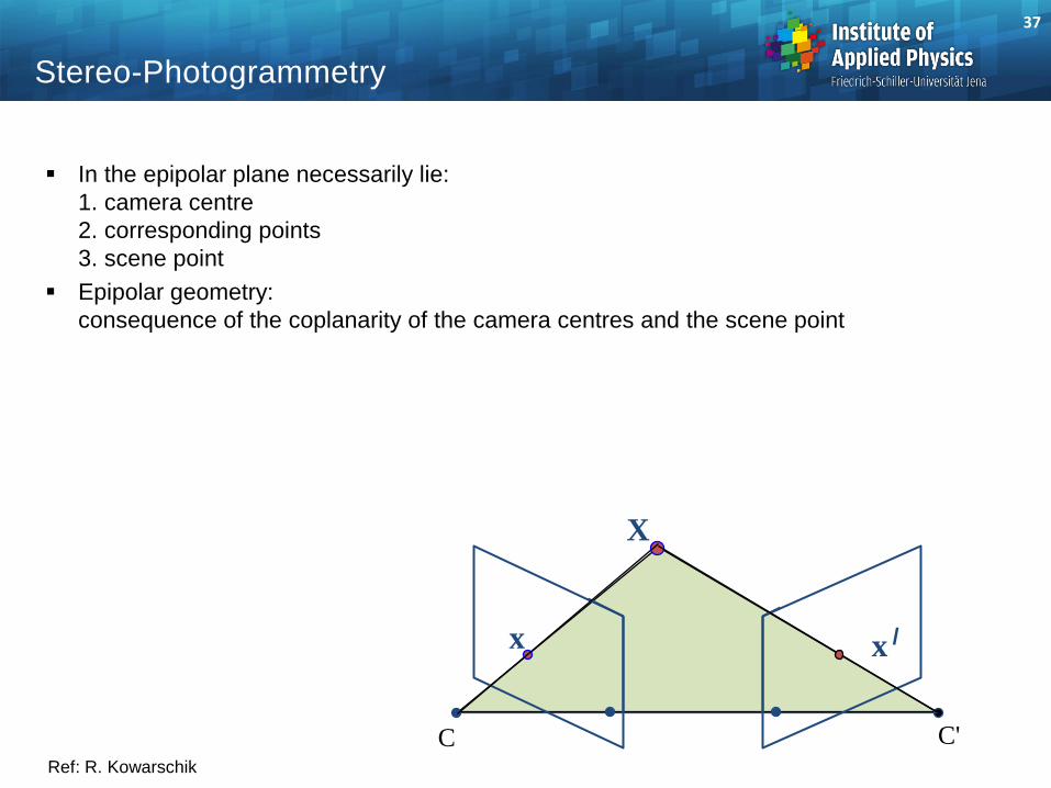
In the epipolar plane necessarily lie:
1. camera centre
2. corresponding points
3. scene point
Epipolar geometry:
consequence of the coplanarity of the camera centres and the scene point
Ref: R. Kowarschik
x x /
X
C C'
38
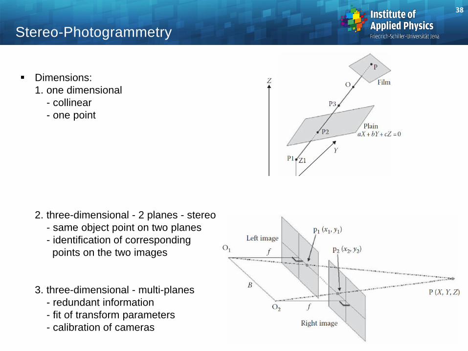
Stereo-Photogrammetry
Dimensions:
1. one dimensional
- collinear
- one point
2. three-dimensional - 2 planes - stereo
- same object point on two planes
- identification of corresponding
points on the two images
3. three-dimensional - multi-planes
- redundant information
- fit of transform parameters
- calibration of cameras
39
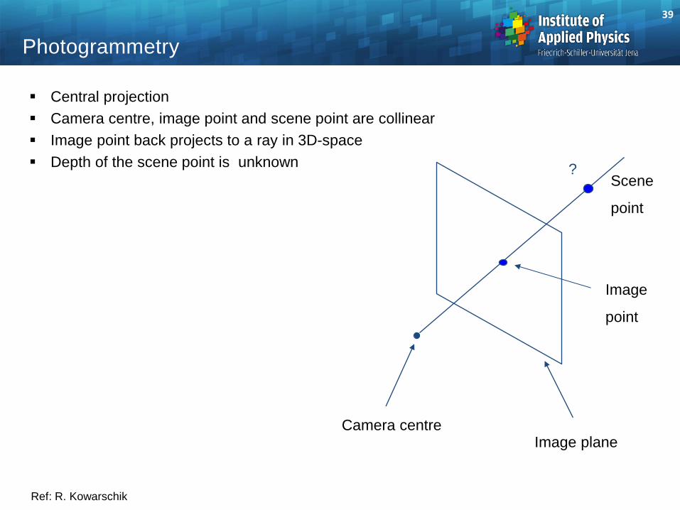
Photogrammetry
Central projection
Camera centre, image point and scene point are collinear
Image point back projects to a ray in 3D-space
Depth of the scene point is unknown
Ref: R. Kowarschik
Camera centre Image plane
Image
point
Scene
point
?
40
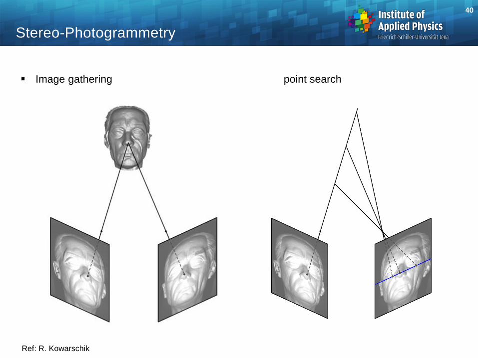
Stereo-Photogrammetry
Image gathering point search
Ref: R. Kowarschik
41
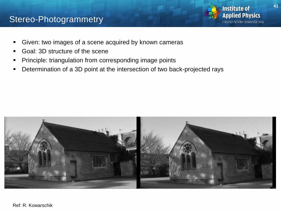
Stereo-Photogrammetry
Given: two images of a scene acquired by known cameras
Goal: 3D structure of the scene
Principle: triangulation from corresponding image points
Determination of a 3D point at the intersection of two back-projected rays
Ref: R. Kowarschik
42
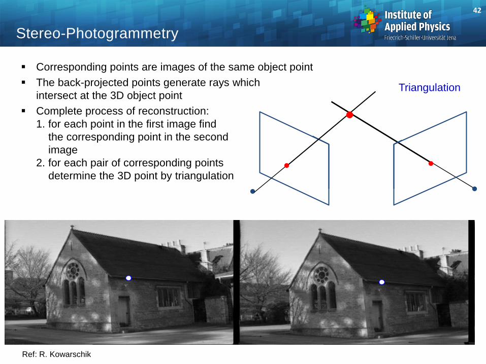
Stereo-Photogrammetry
Corresponding points are images of the same object point
The back-projected points generate rays which
intersect at the 3D object point
Complete process of reconstruction:
1. for each point in the first image find
the corresponding point in the second
image
2. for each pair of corresponding points
determine the 3D point by triangulation
Ref: R. Kowarschik
Triangulation
43
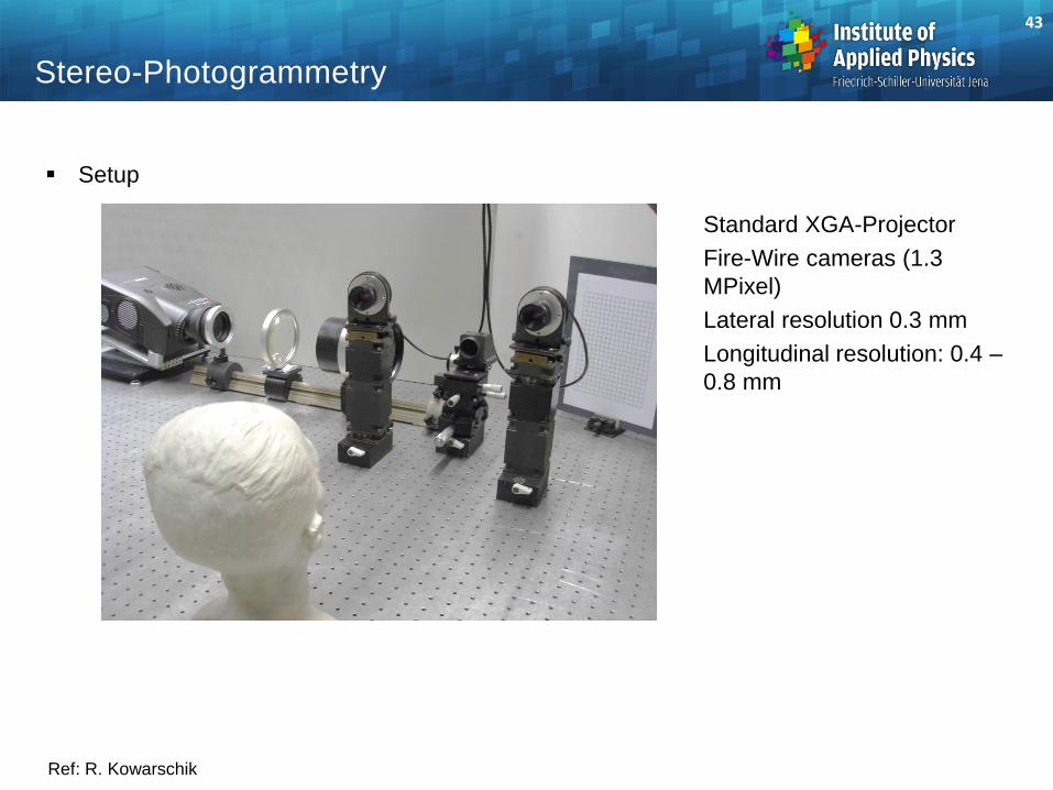
Stereo-Photogrammetry
Setup
Ref: R. Kowarschik
Standard XGA-Projector
Fire-Wire cameras (1.3
MPixel)
Lateral resolution 0.3 mm
Longitudinal resolution: 0.4 –
0.8 mm
44
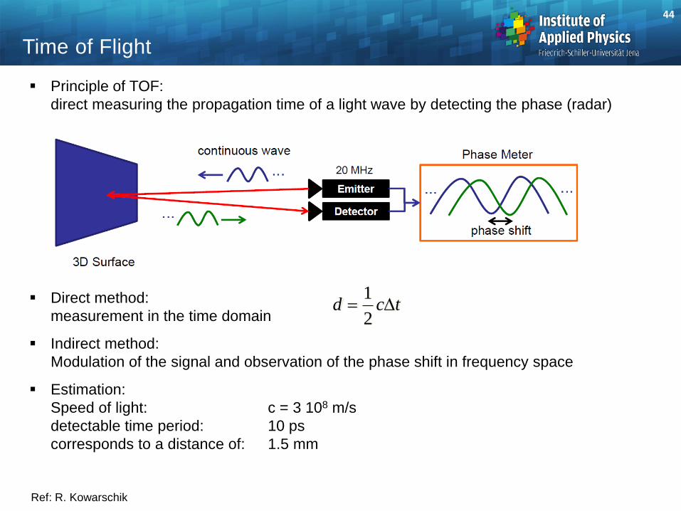
Time of Flight
Principle of TOF:
direct measuring the propagation time of a light wave by detecting the phase (radar)
Direct method:
measurement in the time domain
Indirect method:
Modulation of the signal and observation of the phase shift in frequency space
Estimation:
Speed of light: c = 3 108 m/s
detectable time period: 10 ps
corresponds to a distance of: 1.5 mm
Ref: R. Kowarschik
tcd D2
1
45
Time of Flight: Properties
The success of TOF is strongly related to the electronic capabilities of fast detection:
gating, calibration, charge transfer, time to digital converter,...
Continuous light waves instead of short light pulses possible
Modulation in terms of frequency of sinusoidal waves
Detected wave after reflection has shifted phase
Advantages:
- Large variety of light sources available
- Applicable to different modulation techniques
- Simultaneous range and amplitude images
- Large volume of measurement (up to 100 m)
- Fast
Disadvantages:
- Integration over time required to reduce noise
- Frame rates limited by integration time
- Motion blur caused by long integration time
- Relative low accuracy (> ~ 1...5 mm)
- Exact triggering ~10 ps ...30 ps
- No scaling with volume
Applications: buildings, rooms, security, archeology
Ref: R. Kowarschik
46
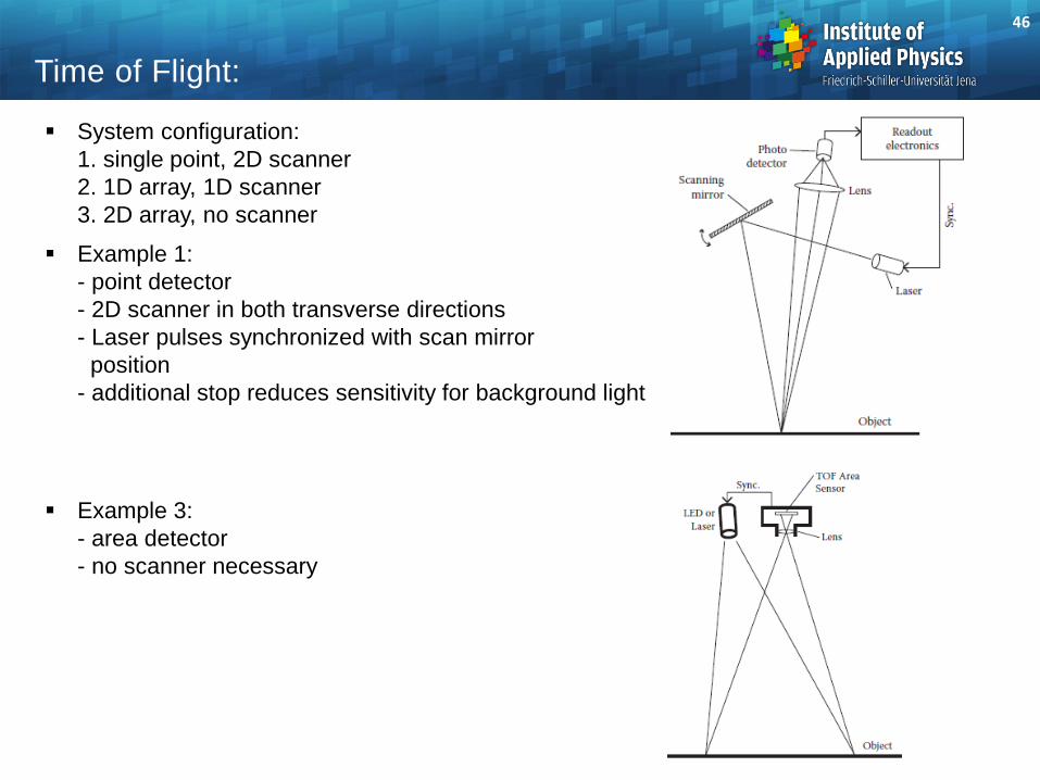
Time of Flight:
System configuration:
1. single point, 2D scanner
2. 1D array, 1D scanner
3. 2D array, no scanner
Example 1:
- point detector
- 2D scanner in both transverse directions
- Laser pulses synchronized with scan mirror
position
- additional stop reduces sensitivity for background light
Example 3:
- area detector
- no scanner necessary
47
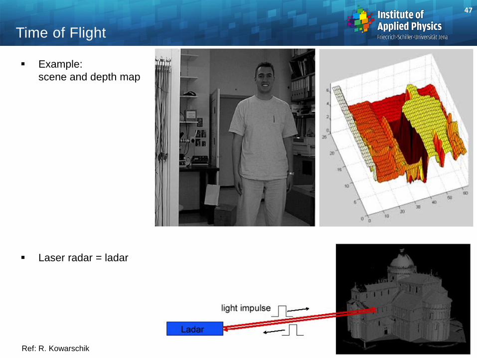
Time of Flight
Example:
scene and depth map
Laser radar = ladar
Ref: R. Kowarschik
48
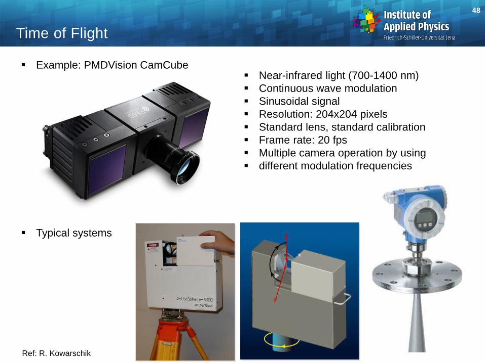
Time of Flight
Example: PMDVision CamCube
Typical systems
Ref: R. Kowarschik
Near-infrared light (700-1400 nm)
Continuous wave modulation
Sinusoidal signal
Resolution: 204x204 pixels
Standard lens, standard calibration
Frame rate: 20 fps
Multiple camera operation by using
different modulation frequencies