metsovo bridge - uni-weimar.de
TRANSCRIPT

Metsovo Bridge
Experimental structural dynamics and Structural monitoring
Bauhaus-Universität Weimar, 19 July 2020 www.uni-weimar.de
Daniela Ardila Ospina (121577)Dulce Mendarte Lopez (121579)

The objective of this project has been to compare the dynamic
response of the Metsovo bridge between a numerical model that has
been developed in SAP2000 software and the data obtained from an
experimental scale test, where the data has been processed using
MATLAB Toolbox MACEC.
1. Objective
19 July 2020
Figure 1: Metsovo Bridge (Costas et al. 2020)

The bridge is located at the Egnatia motorway in Thessaloniki city (Greece). It is composed in its
superstructure with 4 span of prestressed concrete and columns with RC.
In order to obtain the dynamic properties of the system and subsequently the soil-structure
interaction, a model corresponding to a scale of 1:100 is developed during the construction stage.
The created model is not made as concrete, it is generated as steel given the difficulties for its
creation using concrete.
2. Metsovo Bridge
19 July 2020
Figure 2: Modelled segment of the bridge
Figure 3: Test set up

A numerical model is developed in SAP2000.20 software. The
dimensions used are the same as those developed by the
university of Aristotle and Bauhaus.
19 July 2020
[SAP2000 software allows the
element to be modeled as frames,
however, as it is of interest to find
the rotations and torsion of the
elements, the model is carried out
with shell elements. ]
3. Numerical model
Figure 4: Numerical model for Metsovo bridge
Due to the problems generated in the connection of the joints of the 90x90x3 and 100x100x5 sections, a
modification is made using instead of the 100x100 section a 90x90 section but using a thickness of 5 to add
rigidity.
Table 1: Dimensions of the Metsovo bride model

A numerical model is developed in SAP2000.20 software.
19 July 2020
[A mesh was made using as a
reference the joints where the
sensors are located in the modeled
system to subsequently facilitate
their visualization and allow an
effective comparison of the results
in the future.]
Table 2: Mechanical properties: A992fy50
3. Numerical model
The type of steel used is A992Fy50 and its mechanical
properties are specified in table 2.
Figure 5: Numerical model for Metsovo bridge

19 July 2020
Figure 6: Mode shape for first 6 modes
(a) Mode 1(b) Mode 2
(c) Mode 3
(d) Mode 4
3. Numerical model
(e) Mode 5 (f) Mode 6

For the configuration shown in figure 6, the first five modes
with their respective periods and frequencies are presented in
table 3.
19 July 2020
3. Numerical model
Table 3: Modal period and Frequencies for the first 5 modes

The response expressed in accelerations was obtained for the
nodes where the sensors were placed. An example is shown
below, for the sensor placed on the on the right-hand side of
the beam at the top and bottom as shown in figure 8.
19 July 2020
Table 1: Historical seismicity that has affected Popayán
3. Numerical model
Figure 7: Response of the structure, at the top (Right) and bottom (Left)
Top
Bottom
Figure 8: Location sketch of the structureresponses obtained

The excitation mechanism is a hammer used at different points of
the structure (The hammer tip has a force transducer, with a load
cell that can log the time history of the loading to the analyzer).
19 July 2020
4. Test description4.1 Excitation mechanism
4.2 Recording sensors
The accelerometers that have been used in the experiment are Eight
triaxle(Model 356A16 by PCB Piezotronics Inc). These
accelerometers are fixed on the system by means of magnetic
force.
The accelerometers that have been used in the experiment are Eight
triaxle(Model 356A16 by PCB Piezotronics Inc). These
accelerometers are fixed on the system by means of magnetic
force.
It is important to note that the sensors have been placed at the top
and bottom of the bridge model and therefore the direction of the
axes is modified.
4.3 Test structure and sensor arrangement
Figure 9: Axes for the sensors at the top and bottom of the bridge model
(a) At the Top
(b) At the bottom

19 July 2020
4. Test description
4.3 Test structure and sensor arrangement Figure 10 shows the sensor
arrangement and the identification
number used in this report to
facilitate the manipulation of
information.
The first two index in the sensor label
stands for:
RF- Reference sensors
TR- Movable sensors on the Top Right part
of the beam
BR- Movable sensors on the Bottom Right
part of the beam
TL- Movable sensors on the Top Left part
of the beam
BL- Movable sensors on the Bottom left
part of the beam
CL- Movable sensors on the Column
Figure 10: Sensor arrangement
Table 4: Experiment setup circle

19 July 2020
4. Test description
4.4 Analyzer
In each cycle the excitation force and the recorded acceleration
time history in real time are logged in to the analyzer. Table 5
shows the available data, the configuration of the sensors, the
recorded duration and the location where the excitation is carried
out for each of the tests
Table 5: Configuration data

Solar updraft tower, prototype
(f) Modal analysis: Stabilization diagrams
19 July 2020
5. MACEC: A matlab toolbox for
experimental and operational modal
analysis
(c) Signal processing(b) Convert to mcsignal format
(d) Preprocessing: Decimate,
Remove offset and delete chanels
(f) Stochastic Subspace identification
(a) Grid file, Slave file, Surface file
Figure 11: Methodology diagram in MACEC
(g) Modes combination

19 July 2020
The frequencies and damping ratio after the combination
are presented below
Table 6: Frequencies and damping ratios
5. MACEC: A matlab toolbox for
experimental and operational modal
analysis

Solar updraft tower, prototype
Sim
ula
tio
n-
FE
ME
xp
erim
ent-
EM
A
19 July 2020
(1.a) Model (FE) (1.b) Analysis(1.c) Model Characteristics
(2.b) Structural identification(2.c) Model Characteristics
(2.a) System
6. Result comparison
FEM- Finite element methods
EMA- Experimental Modal Analysis
Figure 12: EMA vs FEM comparison process
Solar updraft tower, prototype19 July 2020
6. Result comparison
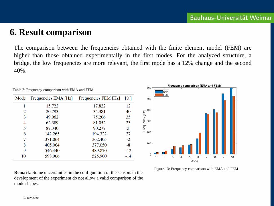
Table 7: Frequency comparison with EMA and FEM
Figure 13: Frequency comparison with EMA and FEM
The comparison between the frequencies obtained with the finite element model (FEM) are
higher than those obtained experimentally in the first modes. For the analyzed structure, a
bridge, the low frequencies are more relevant, the first mode has a 12% change and the second
40%.
Remark: Some uncertainties in the configuration of the sensors in the
development of the experiment do not allow a valid comparison of the
mode shapes.

Solar updraft tower, prototype19 July 2020
6. Result comparison
In order to improve the mathematical model
used and to reduce the difference in the
frequencies obtained, the material properties are
adjusted.
Table 9: Frequency comparison with EMA and FEM
Table 8: Mechanical properties: S235
Figure 14: Frequency comparison with EMA and FEM
Solar updraft tower, prototype19 July 2020
6. Result comparison
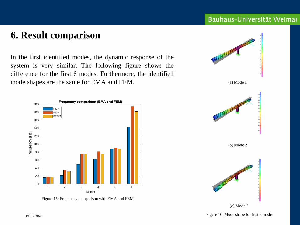
In the first identified modes, the dynamic response of the
system is very similar. The following figure shows the
difference for the first 6 modes. Furthermore, the identified
mode shapes are the same for EMA and FEM.
Figure 15: Frequency comparison with EMA and FEM
(a) Mode 1
(b) Mode 2
(c) Mode 3
Figure 16: Mode shape for first 3 modes

FRF: Contains the dynamic characteristics of thestructure: mass, stiffness, damping, obtained duethe excitation force.
19 July 2020
6. Result comparison
In the EMA graphs can beobserved a greater rangeof frequencies while theFEA graphs show only thefirst frequencies.
Figure 17: FRF at the RF01 Sensor of EMA Figure 18: FRF at the RF01 Sensor of FMA
Figure 19: FRF at the TL04 Sensor of EMAFigure 20: FRF at the TL04 Sensor of FMA
Figure 21: Response function

Solar updraft tower, prototype
6. Result comparison
19 July 2020
Figure 21: Frequencies obtained according to the different configuration of the placed Sensors.

19 July 2020
7. Conclusions
• In order to improve the mathematical model used and to
reduce the difference in the frequencies obtained, the
material properties are adjusted.
• The difficulty of simulating the bridge section at scale for
experimental modal analysis makes it necessary to use
different materials that may lead to a differentiation in the
dynamic response obtained.
• When comparing the results obtained by both approach
(FEM and EMA) in terms of frequency, it is observed how
the resulting in FEM are higher, this may be due to the
difficulty of accurately simulating the scale model
adjusting the dimensions and sections. Nevertheless, the
experimental model may have a contribution by having
errors in data processing. Still, the overall results are close,
and the mode shapes show the same behavior.

Group Members
Daniela Ardila Ospina
NHRE Master Student
Bauhaus Universität Weimar
Colombia
Solar updraft tower, prototype
Dulce Mendarte Lopez
NHRE Master Student
Bauhaus Universität Weimar
Mexico
19 July 2020
References
Costas, Argyris, Papadimitriou Costas, Panetsos Panagiotis, y Tsopelas Panos. 2020. «Bayesian
Model-Updating Using Features of Modal Data: Application to the Metsovo Bridge», junio, 25.
Solar updraft tower, prototype19 July 2020

Thank you for your attention!
Bauhaus-Universität Weimar, 19 July 2020 www.uni-weimar.de www.uni-weimar.de/bauhaus100