This content has been downloaded from IOPscience. Please scroll down to see the full text.

Download details:

IP Address: 137.207.120.173

This content was downloaded on 11/11/2014 at 20:10

Please note that terms and conditions apply.

MHV techniques for QED processes

View the table of contents for this issue, or go to the journal homepage for more

JHEP11(2005)016

(http://iopscience.iop.org/1126-6708/2005/11/016)

Home Search Collections Journals About Contact us My IOPscience

JHEP11(2005)016

Published by Institute of Physics Publishing for SISSA

Received: October 3, 2005

Accepted: October 30, 2005

Published: November 14, 2005

MHV techniques for QED processes

Kemal J. Ozeren and W. James Stirling

Institute for Particle Physics Phenomenology

University of Durham, DH1 3LE, U.K.

E-mail: kemal.ozeren@durham.ac.uk, w.j.stirling@durham.ac.uk

Abstract: Significant progress has been made in the past year in developing new ‘MHV’

techniques for calculating multiparticle scattering amplitudes in Yang-Mills gauge theories.

Most of the work so far has focussed on applications to Quantum Chromodynamics, both

at tree and one-loop level. We show how such techniques can also be applied to abelian

theories such as QED, by studying the simplest tree-level multiparticle process, e+e− → nγ.

We compare explicit results for up to n = 5 photons using both the Cachazo, Svrcek and

Witten ‘MHV rules’ and the related Britto-Cachazo-Feng ‘recursion relation’ approaches

with those using traditional spinor techniques.

Keywords: Duality in Gauge Field Theories, Electromagnetic Processes and Properties,

QCD.

c© SISSA 2005 http://jhep.sissa.it/archive/papers/jhep112005016/jhep112005016.pdf

JHEP11(2005)016

Contents

1. Introduction 1

2. KS approach to e+e− → nγ 2

3. MHV and MHV amplitudes 3

3.1 Photons 4

4. The MHV rules 5

4.1 Simple examples 6

4.2 The NMHV amplitude A(f+1 , f−

2 , 3+, 4+, 5−, 6−) 8

4.3 Soft limits 9

5. The BCF recursion relations 10

5.1 Example of BCF recursion relations applied to a QED process 11

5.2 The NMHV amplitude A(f+1 , f−

2 , 3+, 4+, 5−, 6−) 12

6. Conclusions 13

A. Notation and conventions 13

B. Proof of the recursion relations 14

1. Introduction

Until recently, the calculation of cross sections for the production of many particles (quarks,

gluons, photons, etc.) in high-energy collisions has been restricted by the technical difficul-

ties associated with the evaluation of the corresponding multiparticle Feynman diagrams.

Significant progress has been made in the past year with the development of new techniques,

principally the ‘MHV rules’ introduced by Cachazo, Svrcek and Witten (CSW) [1] and the

Britto-Cachazo-Feng (BCF) [2] recursion relations, in which amplitudes are constructed

from a new set of building blocks — Maximum Helicity Violating (MHV) amplitudes —

which themselves represent groups of Feynman diagrams corresponding to particular exter-

nal helicity configurations. In contrast to the usual approach, the amplitudes are expressed

in terms of positive and negative chirality spinors (λ and λ) and their corresponding prod-

ucts. The MHV amplitudes have very simple expressions in terms of these spinor products,

which replace the usual scalar products pi · pj as the means by which the scattering ampli-

tudes depend on the external particle four-momenta. Although first used to calculate tree

amplitudes, these techniques have since been successfully applied at 1-loop [3].

– 1 –

JHEP11(2005)016

So far, the focus of attention has been on developing and exploiting techniques for QCD

scattering processes, for example gg → ng, gg → qq + ng etc., since such amplitudes are

needed to estimate multi-jet cross sections at hadron colliders. Indeed, the MHV rules [1]

were specifically developed for and applicable to massless Yang-Mills field theory.

In this paper we investigate whether similar techniques exist for abelian field theo-

ries, in particular QED. We choose as our test-bed process the simplest QED tree-level

multiparticle scattering process, e+e− → nγ.1

In fact the e+e− → nγ process was already studied [4] almost twenty years ago at a

time when ‘spinor techniques’ for scattering amplitudes were being developed. The process

was used to illustrate the power of these new techniques; extremely compact expressions

were obtained for the production of arbitrary numbers of photons, even taking the non-zero

electron mass into account. We will refer to this as the KS approach. The expressions were

specifically designed to allow for efficient numerical computation of the amplitudes, and

indeed the only limitation on the size of n was due to the available computing power at

the time.

It is therefore interesting to see whether the more modern MHV-based techniques

can improve on the calculational efficiency of the original KS expressions. This can be

measured, for example, by the compactness of the algebraic expressions and by the time

taken to evaluate the spin-summed amplitude squared for one ‘event’ corresponding to a

random point in phase space.

The paper is organised as follows. In the next section 2 we summarise the results of

ref. [4] for the (massless) e+e− → nγ scattering ampplitude. We then repeat the calculation

using the QED-generalised version of the MHV technique, both in the original MHV-rules

and recursive (BCF) approaches.

2. KS approach to e+e− → nγ

Consider the process

e−(pa) + e+(pb)→ γ(k1) + γ(k2) + · · ·+ γ(kn) . (2.1)

In the massless (electron) limit, helicity is conserved at each fermion-photon vertex and

so the helicities of the electron and positron will be opposite, he− = −he+ . There are

therefore 2n+1 distinct spin amplitudes (two polarisations for each photon and he− = ±).

In the traditional approach, the (n!) Feynman diagrams are obtained simply by joining the

n photons to the fermion line in all possible ways. Labelling the distinct polarisation states

by S = 1, . . . , 2n+1 gives an expression for the unpolarised cross section of

dσn =1

F[dΦn]

1

n!

1

4

∑

S

|MS |2 , (2.2)

where the terms on the right-hand side are the flux factor, the phase space volume element,

the symmetry factor and the spin-summed/averaged amplitude squared respectively.

1There is of course no tree-level QED analogue of the QCD process gg → ng.

– 2 –

JHEP11(2005)016

The KS result is2 [4]

MS = en

n∏

j=1

p · kj

−1/2n!∑

D=1

〈pa a1〉 [pb bn]×n−1∏

i=1

{〈qi ai+1〉 [qi bi]

q2i

+〈p ai+1〉 [p bi]

2p · qi

}, (2.3)

where pµ is an arbitrary light-like four vector and

ai = p , bi = ki if hi = + ,

ai = ki , bi = p if hi = − . (2.4)

The sum in (2.3) is over the n! distinct permutations k1, k2, . . . of the photon momenta

k1, k2, . . . , from which internal four-momenta are defined by

qi =

i∑

j=1

kj − pa , i = 1, . . . , n (qn ≡ pb) ,

qi = qi −q2i

2p · qipi , (q2

i = 0) . (2.5)

The 〈ij〉 and [ij] spinor products that appear in eq. (2.3) are defined in appendix A. The

full expression for the amplitude for arbitrary n can then be written in just a few lines

of computer code. Note that the result for the amplitude squared is independent of pµ

(which is related to the choice of photon gauge) and this provides a powerful check on the

calculational procedure.

3. MHV and MHV amplitudes

Particular helicity amplitudes in Yang-Mills theory take on unexpectedly simple forms.

This is despite the considerable computational effort involved in their calculation via the

standard Feynman diagram approach. Long expressions involving many terms often sim-

plify to a single term, or even vanish. At tree level for example, purely gluonic colour-

ordered scattering amplitudes can be summarized as follows:3

A(1+, 2+, . . . , n+) = 0

A(1+, 2+, . . . , i−, . . . , n+) = 0 (3.1)

A(1+, 2+, . . . , i−, . . . , j−, . . . , n+) =〈i j〉4∏n

k=1〈k k + 1〉 .

So amplitudes with all the gluons having the same helicity vanish, as do those with only one

gluon having a different helicity to the others. The third case above therefore corresponds to

maximally helicity violating (MHV) amplitudes. Their simple form was first conjectured by

2This expression corresponds to the choice he− = −. The corresponding h

e− = + amplitudes are readily

obtained using parity invariance.3All particles are incoming, and the coupling constant factors have been omitted. The spinor products

〈. . . 〉 are defined in appendix A.

– 3 –

JHEP11(2005)016

Parke and Taylor [5], and later proven by Berends and Giele [6] using a recursive technique.

Note that A(1+, 2+, . . . , i−, . . . , j−, . . . , n+) above is called a ‘mostly plus’ MHV amplitude,

for obvious reasons. Its ‘mostly minus’ counterpart, which has two positive helicities and

the remainder negative, is called an MHV amplitude, and can be obtained simply by

interchanging 〈..〉 → [. . . ].

3.1 Photons

The main difference when we consider QED is that there are no pure-photon tree-level

amplitudes. There must always be (at least) one pair of fermions present, which must be

of opposite helicity due to our convention that all particles are incoming. Also, in contrast

to non-abelian theories there is no concept of colour ordering, so we will be concerned with

full physical amplitudes rather than colour-ordered partial amplitudes. It is again the case

that amplitudes with only one negative helicity particle (which must be either the fermion

or anti-fermion — we shall take it to be the former) vanish,

AQED(f+, f−, 1+, 2+, . . . , I+, . . . , n+) = 0 . (3.2)

Here i+ denotes a positive helicity photon with momentum pi, and f , f denote fermion

and anti-fermion respectively. The MHV amplitudes take the following form (for massless

fermions):

AQED(f+, f−, 1+, 2+ . . . , I−, . . . , n+) =

2n

2 en〈ff〉n−2〈fI〉3〈fI〉∏nk=1〈fk〉〈fk〉

. (3.3)

This is the fundamental MHV amplitude in QED, and as before it consists of only a single

term. The factor en is the gauge coupling constant, which we will normally omit in what

follows. It is possible [7] to obtain the amplitude in (3.3) by symmetrizing colour-ordered

non-abelian amplitudes,

AQED(f, f, 1, 2, 3, . . . , n

)= A

(f, f, 1, 2, 3, . . . , n

)+ A

(f, f, 2, 1, 3, . . . , n

)+ · · · . (3.4)

Each term on the right-hand side is a colour-ordered MHV (Parke-Taylor) QCD amplitude,

and we sum over n! permutations of n gluons. A factor of 2n

2 must also be included to take

account of different generator normalizations — our QED generators are normalized to 1.

It should be noted that in writing (3.3) in this particular way we have made an apparently

arbitrary choice of phase. Since the phase of a full (i.e. not partial) amplitude is not a

physical observable, any of the 〈. . . 〉 products in (3.3) could, naively, be replaced with the

corresponding [. . . ] product. We will come back to this point later. It is worth mentioning

that due to parity invariance the amplitude with all the helicities flipped has the same

magnitude as (3.3) above. Also, one can use charge conjugation invariance to switch the

fermion and anti-fermion.

– 4 –

JHEP11(2005)016

We can write (3.3) in a physically more illuminating way, emphasizing the pole struc-

ture:

A(f

+, f−, 1+, 2+ . . . , I−, . . . , n+

)=〈fI〉3〈fI〉〈ff〉2

n∏

k=1

e√

2〈ff〉〈fk〉〈fk〉

(3.5)

=〈fI〉3〈fI〉〈ff〉2

n∏

k=1

Sk . (3.6)

It is a fundamental result of general quantum field theories that scattering amplitudes have

a universal behaviour in the soft (gauge boson) limit. When all components of a particular

photon’s momentum are taken to zero, the amplitude factorizes into the amplitude in the

absence of that photon multiplied by an ‘eikonal factor’,

Sk =e√

2〈ff〉〈fk〉〈fk〉

. (3.7)

The form of this factor is universal. Since the QED MHV amplitude is just a single term,

it follows that the eikonal factors must be present as factors — and indeed they are.

4. The MHV rules

There has been much recent progress in calculating scattering amplitudes in perturbative

Yang-Mills theory. Cazacho, Svrcek and Witten [1] introduced a novel diagrammatic tech-

nique, known as the ‘MHV rules’, in which maximally helicity violating (MHV) amplitudes

are used as vertices in a scalar perturbation theory. These vertices are connected by scalar

propagators 1/p2. This arrangement vastly reduces the number of diagrams that must be

evaluated relative to the traditional Feynman rules case.

Although the original CSW paper dealt only with purely gluonic amplitudes, the for-

malism has been successfully extended to include quarks [8, 9], Higgs [10] and massive gauge

bosons [11]. In this paper we will use (3.3) to apply the MHV rules to QED processes,

and derive relatively simple formulae for four and five photon amplitudes (an electron and

positron are understood to be present also).

In order to use MHV amplitudes as vertices, it is necessary to continue them off-shell,

since internal momenta will not be light-like. We need to define spinors λ for the internal

lines. The convention established in [1], which we shall follow, defines λ to be

λa = paaηa (4.1)

for an internal line of momentum paa, where ηa is arbitrary. The same η must be used for

all internal lines and in all diagrams contributing to a particular amplitude. In practice, it

proves convenient to choose η to be one of the conjugate (opposite chirality) spinors λ of

the external fermion legs. Note that for external lines, which remain on-shell, λ is defined

in the usual way (see appendix A).

Having defined the MHV amplitudes, and the manner in which they are to be continued

off-shell, we are now in a position to calculate non-MHV amplitudes. These are simply

those with more than two negative-helicity particles.

– 5 –

JHEP11(2005)016

←− q

1+

4−

3−

2−

− +

Figure 1: Diagram contributing to A(f+

1 , f−

2 , 3−, 4−). Fermion lines are dashed, photon lines are

solid. All particles are incoming. There is also a similar diagram with photons 3 and 4 interchanged.

4.1 Simple examples

As a first example let us calculate A(f+1 , f−

2 , 3−, 4−).4 This is expected to vanish, see (3.2).

There are two contributing MHV diagrams, though they differ only by a permutation of

photons. Note that the external legs are not constrained to be positioned cyclically as in

the case of colour-ordered partial amplitudes. The absence of a pure-photon vertex means

that the internal lines of MHV diagrams for QED processes with two fermions can only be

fermionic. The contribution of the diagram in figure 1 can be written down immediately as

√2〈λq 4〉2〈λq 1〉

1

q2

√2〈2 3〉2〈2 λq〉

, (4.2)

where λq is the spinor representing the internal line of momentum q. This expression is

simply a product of two MHV vertices and a propagator. Using (4.1) we can evaluate the

spinor products involving λq:

〈λq 4〉 = 〈4 1〉 φ1 ,

〈λq 1〉 = 〈1 4〉 φ4 ,

〈2 λq〉 = 〈2 3〉 φ3 ,

q2 = (k2 + k3)2 ,

= 〈2 3〉[2 3] . (4.3)

Here φi = [η i] is a function of the (arbitrary) spinor η. Simplifying, we find

−2〈4 1〉[2 3]

φ21

φ3φ4

. (4.4)

To this we must add the contribution from the diagram with photons 3 and 4 interchanged,

namely

−2〈3 1〉[2 4]

φ21

φ4φ3

. (4.5)

4Note the change in notation — the spinor representing the fermion is now denoted 2 (not f) and the

spinor representing the anti-fermion is now denoted 1 (not f). Also, for clarity we will now omit the coupling

constants.

– 6 –

JHEP11(2005)016

←− q

1+

5+

3−

2−

− +

4− ←− r

1+

4−

− +

5+

3−

2−

(a) M (b) N

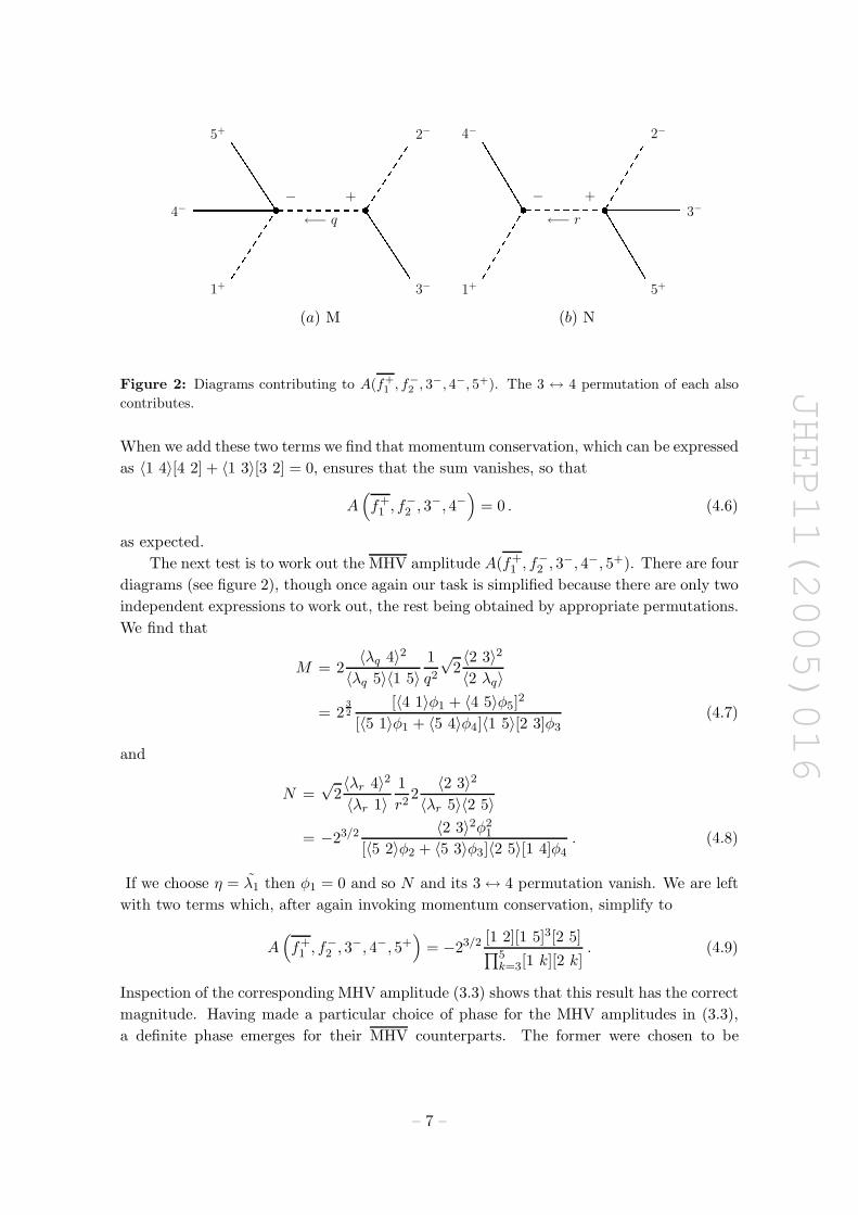
Figure 2: Diagrams contributing to A(f+

1 , f−

2 , 3−, 4−, 5+). The 3 ↔ 4 permutation of each also

contributes.

When we add these two terms we find that momentum conservation, which can be expressed

as 〈1 4〉[4 2] + 〈1 3〉[3 2] = 0, ensures that the sum vanishes, so that

A(f+1 , f−

2 , 3−, 4−)

= 0 . (4.6)

as expected.

The next test is to work out the MHV amplitude A(f+1 , f−

2 , 3−, 4−, 5+). There are four

diagrams (see figure 2), though once again our task is simplified because there are only two

independent expressions to work out, the rest being obtained by appropriate permutations.

We find that

M = 2〈λq 4〉2〈λq 5〉〈1 5〉

1

q2

√2〈2 3〉2〈2 λq〉

= 23

2[〈4 1〉φ1 + 〈4 5〉φ5]

2

[〈5 1〉φ1 + 〈5 4〉φ4]〈1 5〉[2 3]φ3

(4.7)

and

N =√

2〈λr 4〉2〈λr 1〉

1

r22〈2 3〉2

〈λr 5〉〈2 5〉

= −23/2 〈2 3〉2φ21

[〈5 2〉φ2 + 〈5 3〉φ3]〈2 5〉[1 4]φ4

. (4.8)

If we choose η = λ1 then φ1 = 0 and so N and its 3↔ 4 permutation vanish. We are left

with two terms which, after again invoking momentum conservation, simplify to

A(f+1 , f−

2 , 3−, 4−, 5+)

= −23/2 [1 2][1 5]3[2 5]∏5

k=3[1 k][2 k]. (4.9)

Inspection of the corresponding MHV amplitude (3.3) shows that this result has the correct

magnitude. Having made a particular choice of phase for the MHV amplitudes in (3.3),

a definite phase emerges for their MHV counterparts. The former were chosen to be

– 7 –

JHEP11(2005)016

holomorphic functions of the λ’s of the external legs — they contain only 〈..〉 products. The

latter emerge as anti-holomorphic, consisting only of [..] products. Colour-ordered partial

amplitudes also have this property. Here however, we are dealing with a physical amplitude,

and so the phase is not a measurable quantity. It is interesting to note that choosing the

MHV amplitudes to have different phases, for instance an expression containing a mixture

of λ and λ, does not in general lead to correct results for non-MHV amplitudes. This is to

be expected, as it is only those amplitudes which, apart from the momentum-conserving

delta function, are comprised entirely of 〈..〉 products that transform simply onto a line in

twistor space [12].

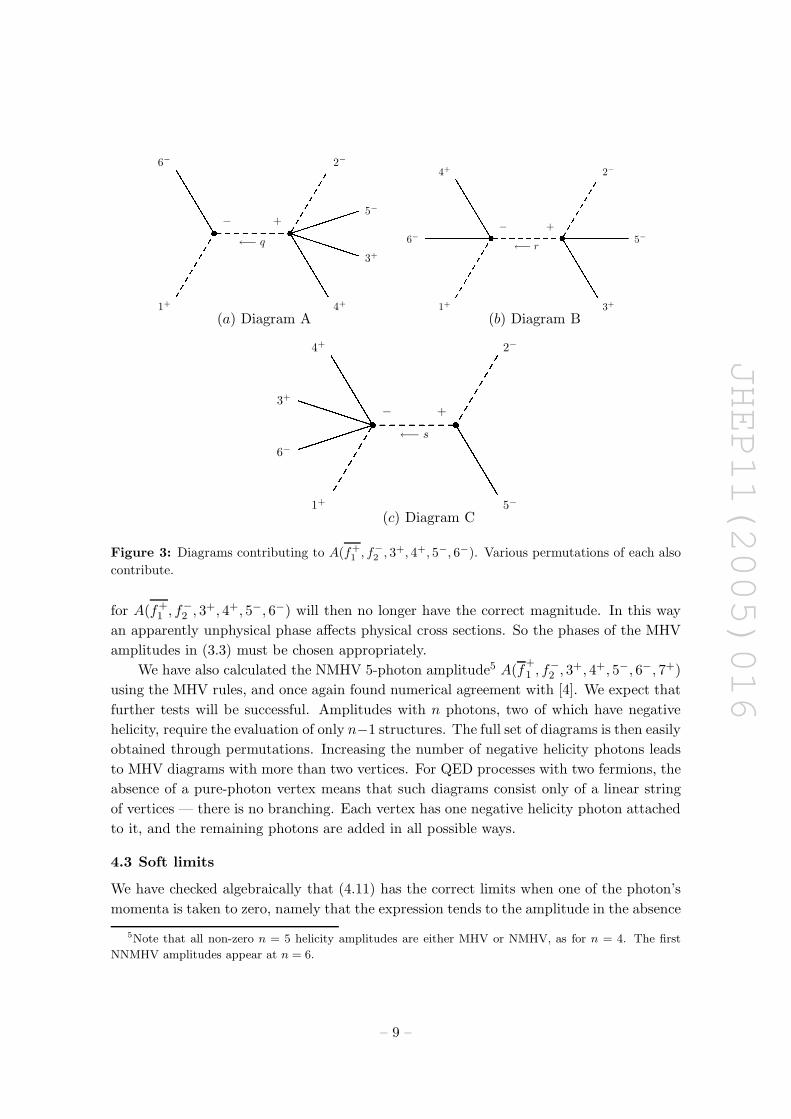
4.2 The NMHV amplitude A(f+1 , f−

2 , 3+, 4+, 5−, 6−)

The first non-zero NMHV amplitudes appear for n = 4 photons, when two photons have

helicity + and two have helicity −. There are eight diagrams for this process but only three

distinct structures, so that we need only work out three diagrams and obtain the others by

permuting photons. In fact, by a judicious choice of the arbitrary spinor η we can reduce

the expression to just two independent terms plus permutations. Referring to figure 3,

A = −4φ2

1[〈2 1〉φ1 + 〈2 6〉φ6]〈2 5〉2[1 6]φ6〈2 3〉〈2 4〉[〈3 1〉φ1 + 〈3 6〉φ6][〈4 1〉φ1 + 〈4 6〉φ6]

,

B = −4[〈6 1〉φ1 + 〈6 4〉φ4]

2〈2 5〉2[〈4 1〉φ1 + 〈4 6〉φ6][〈3 2〉φ2 + 〈3 5〉φ5]〈1 4〉r2〈2 3〉 ,

C = −4[〈1 2〉φ2 + 〈1 5〉φ5][〈6 2〉φ2 + 〈6 5〉φ5]

2

[〈3 2〉φ2 + 〈3 5〉φ5][〈4 2〉φ2 + 〈4 5〉φ5]〈1 3〉〈1 4〉[2 5]φ5

. (4.10)

If we choose η = λ1 then φ1 = 0 and the contribution from diagram A above vanishes.

The other two terms simplify, and we end up with the following expression,

A(f+1 , f−

2 , 3+, 4+, 5−, 6−) = 4〈4 6〉[1 4]2〈2 5〉2

〈1 4〉[1 6](p2 + p3 + p5)2〈2 3〉〈3|2 + 5|1] +

+ (3↔ 4) + (5↔ 6) +

(3↔ 4

5↔ 6

)+

+ 4(s12 + s15)〈6|2 + 5|1]2

〈1 3〉〈1 4〉[5 2][1 5]〈3|2 + 5|1]〈4|2 + 5|1] +

+ (5↔ 6) (4.11)

The notation 〈i | j + k | l ] and sij is defined in appendix A. Although the two algebraic

forms are very different, we have checked that this expression agrees numerically with the

KS results [4], up to a phase. It is interesting to note that we do not have the freedom to

introduce relative phases among the set of MHV amplitudes. For example, introducing a

factor of −1 into the 1-photon MHV amplitude while leaving the others fixed will obviously

lead to a change in the relative phases among the terms in (4.11). Our derived expression

– 8 –

JHEP11(2005)016

←− q

1+

6−

− +

4+

3+

5−

2−

←− r

1+

6−

4+

− +

3+

5−

2−

(a) Diagram A (b) Diagram B

←− s

5−

2−

+−

1+

6−

3+

4+

(c) Diagram C

Figure 3: Diagrams contributing to A(f+

1, f−

2, 3+, 4+, 5−, 6−). Various permutations of each also

contribute.

for A(f+1 , f−

2 , 3+, 4+, 5−, 6−) will then no longer have the correct magnitude. In this way

an apparently unphysical phase affects physical cross sections. So the phases of the MHV

amplitudes in (3.3) must be chosen appropriately.

We have also calculated the NMHV 5-photon amplitude5 A(f+

1 , f−2 , 3+, 4+, 5−, 6−, 7+)

using the MHV rules, and once again found numerical agreement with [4]. We expect that

further tests will be successful. Amplitudes with n photons, two of which have negative

helicity, require the evaluation of only n−1 structures. The full set of diagrams is then easily

obtained through permutations. Increasing the number of negative helicity photons leads

to MHV diagrams with more than two vertices. For QED processes with two fermions, the

absence of a pure-photon vertex means that such diagrams consist only of a linear string

of vertices — there is no branching. Each vertex has one negative helicity photon attached

to it, and the remaining photons are added in all possible ways.

4.3 Soft limits

We have checked algebraically that (4.11) has the correct limits when one of the photon’s

momenta is taken to zero, namely that the expression tends to the amplitude in the absence

5Note that all non-zero n = 5 helicity amplitudes are either MHV or NMHV, as for n = 4. The first

NNMHV amplitudes appear at n = 6.

– 9 –

JHEP11(2005)016

of that photon, multiplied by a ‘soft’ factor called the eikonal factor:

A(f+1 , f−

2 , 3+, 4+, 5−, 6−)3→0−→ A(f+

1 , f−2 , 4+, 5−, 6−)×

√2〈1 2〉

〈1 3〉〈2 3〉

A(f+1 , f−

2 , 3+, 4+, 5−, 6−)5→0−→ A(f+

1 , f−2 , 3+, 4+, 6−)×

√2[1 2]

[1 5][2 5](4.12)

and similarly for the other photons. Notice that when a positive helicity photon becomes

soft, the eikonal factor is comprised entirely of 〈. . . 〉 spinor products, whereas when a neg-

ative helicity photon becomes soft the eikonal factor is comprised entirely of [. . . ] products.

We have also verified that the MHV amplitudes (3.3) have the correct collinear factoriza-

tion properties when one of the photons is emitted in the direction of the incoming fermion

or anti-fermion.6

5. The BCF recursion relations

A new set of recursion relations [2] has been proposed to calculate tree amplitudes in gauge

theories. We will here give a brief review of this technique, before showing how the relations

can be used, along with (3.3), to calculate QED amplitudes.

Consider an n particle (say gluonic, for definiteness) scattering amplitude, with ar-

bitrary helicities. Choose two of the external lines to be ‘hatted’ — this will be defined

shortly. Suppose the n-th (positive helicity) and (n − 1)-th (negative helicity) gluons are

hatted. These are reference lines. The BCF recursion relation then reads

An(1, 2, . . . , (n− 1)−, n+) = (5.1)

=n−3∑

i=1

∑

h=+,−

Ai+2

(n, 1, 2, . . . , i,−P h

n,i

) 1

P 2n,i

An−i

(+P−h

n,i , i + 1, . . . , n− 2, n − 1)

,

where

Pn,i = pn + p1 + · · ·+ pi ,

Pn,i = Pn,i +P 2

n,i

〈n− 1|Pn,i|n]λn−1λn ,

pn−1 = pn−1 −P 2

n,i

〈n− 1|Pn,i|n]λn−1λn ,

pn = pn +P 2

n,i

〈n − 1|Pn,i|n]λn−1λn . (5.2)

Identities such as

〈• P 〉 = −〈• | P | n]× 1

ω,

[P •] = −〈n− 1 | P |•]× 1

ω, (5.3)

6The collinear behaviour of QCD MHV amplitudes has been studied in [13].

– 10 –

JHEP11(2005)016

2−

4+

5−

3+

1+

+

−

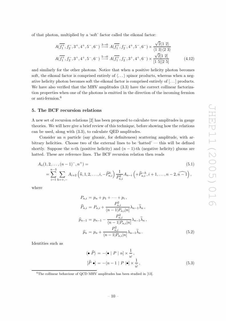
Figure 4: BCF Diagram contributing to A(f+

1 , f−

2 , 3+, 4+, 5−). As usual, dashed lines are fermions,

solid lines are photons.

where ωω = 〈n−1 |P |n] (the factors ω and ω only ever appear together in this combination)

are used to remove the hats, whereupon the result can be simplified using standard spinor

identities. The procedure can be conveniently represented diagrammatically, see figure 4

for a specific case.

In ref. [14] the relations were shown to work for amplitudes involving fermions, and in

ref. [15] it was shown that the reference gluons need not be either adjacent or of the same

helicity. Applications to massive particles were described in [16]. The relations were proven

in [15] by shifting the hatted momenta by a complex amount — see appendix B. Here we

will be interested in applying the above recursion relation to QED processes. In contrast

to the MHV rules, the recursion relations involve the use of MHV amplitudes. We can

obtain these from (3.3) by switching 〈..〉 and [..], and using charge conjugation invariance

to swap the fermion and anti-fermion.

5.1 Example of BCF recursion relations applied to a QED process

Consider the MHV amplitude A(f+

1 , f−2 , 3+, 4+, 5−). As before, f and f denote a fermion

and anti-fermion respectively, and i+ represents a positive helicity photon of momentum

ki. Let us choose the hatted lines to be 1 and 5, as shown in Figure 4. Then there is only

one distinct diagram7 for this process, which evaluates to

√2[1 3]2

[1 P ]

1

(k1 + k3)22〈2 5〉2

〈2 4〉〈P 4〉. (5.4)

Here we have used (3.3), together with its helicity flipped version, to substitute for the (on-

shell) tree amplitudes in (5.1). P = k1+k3 is the momenta of the internal line. Simplifying,

we get

2√

2〈2 5〉2

〈2 4〉〈3 4〉〈1 3〉 , (5.5)

7Note that as detailed in [2], diagrams with an upper vertex of (+ + −) or a lower vertex of (− − +)

vanish. We have not drawn such diagrams.

– 11 –

JHEP11(2005)016

2−

4+

6−

5−

3+

1+

+

−

2−

4+

5−

3+

6−

1+

+

−

2−

5−

6−

4+ 3+

1+

+

−

(a) Diagram P (b) Diagram Q (c) Diagram R

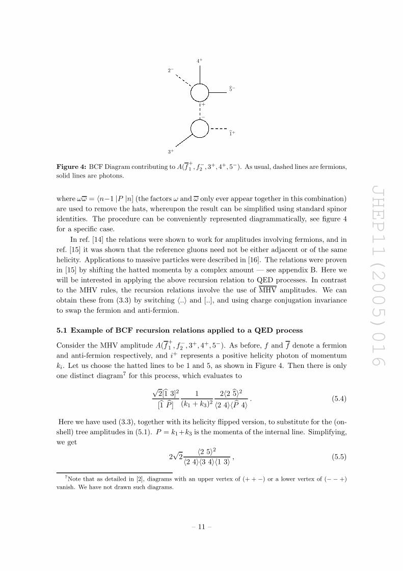
Figure 5: BCF diagrams contributing to A(f+

1 , f−

2 , 3+, 4+, 5−, 6−). Various permutations of each

also contribute.

and to this we must add a similar expression with photons 3 and 4 interchanged,

2√

2〈2 5〉2

〈2 3〉〈4 3〉〈1 4〉 . (5.6)

After simplifying using Schouten’s identity8 we recover the expected result,

A(f+

1 , f−2 , 3+, 4+, 5−) = 2

√2

〈2 5〉2〈2 4〉〈3 4〉〈1 3〉 + 2

√2

〈2 5〉2〈2 3〉〈4 3〉〈1 4〉

= 2√

2〈2 1〉〈2 5〉3〈1 5〉∏5

k=3〈1 k〉〈2 k〉. (5.7)

5.2 The NMHV amplitude A(f+1 , f−

2 , 3+, 4+, 5−, 6−)

There are three BCF diagrams for this process, up to permutations, which is the same one

that we calculated in section 4.2 using the MHV rules. We can build up the four photon

process using amplitudes we have already calculated. The diagrams (figure 5) evaluate to

P = 4〈5|1 + 3|2]〈5|1 + 3|4]2

〈3|1 + 5|2]〈5|1 + 3|6](p1 + p3 + p5)2[2 6]〈1 3〉 ,

Q = 4〈2 5〉2[3 1]2〈5|3 + 6|1]

〈2 4〉〈4|3 + 6|1]〈5|1 + 3|6](p1 + p3 + p6)2[6 1]

R = 4〈6|2 + 5|1]2(p1 + p2 + p5)

2[2 1]2

〈3|2 + 5|1]〈4|2 + 5|1]〈3|1 + 5|2]〈4|1 + 5|2][5 1][2 5], (5.8)

where we have chosen external lines 1 and 5 to be hatted. The full result is then

A(f+1 , f−

2 , 3+, 4+, 5−, 6−) = (P + Q) + (3↔ 4) + R . (5.9)

We have checked numerically that this expression is equal to (4.11) which was calculated

using the MHV rules. Both are equal to the corresponding result obtained from the KS

formula, up to a phase.

8For any 4 spinors 〈a b〉〈c d〉 + 〈a c〉〈d b〉 + 〈a d〉〈b c〉 = 0.

– 12 –

JHEP11(2005)016

6. Conclusions

We have shown that the modern techniques inspired by the transformation of Yang-Mills

scattering amplitudes to twistor space [12] can be successfully applied to QED processes,

and yield reasonably compact expressions. As well as some simple MHV amplitudes, we

calculated the NMHV amplitude A(f+1 , f−

2 , 3+, 4+, 5−, 6−) using both the MHV rules and

BCF recursion approaches. The expressions obtained are not obviously equal, but numer-

ical checks proved them to be so and the results were confirmed by comparison with the

KS [4] formula, which is directly derived from Feynman diagrams. We have also checked

that the amplitudes have the correct factorising (eikonal) form when one of the photons

becomes soft. Note that the QED NMHV amplitudes we have presented can also in prin-

ciple be obtained by symmetrizing QCD colour-ordered amplitudes, but this is a laborious

procedure and will not lead directly to compact expressions. We have shown that it is

possible, and much easier, to use physical MHV amplitudes directly in the MHV rules.

We have given explicit expressions for up to and including 4-photon amplitudes. The

extension to n ≥ 5 photons is in principle straightforward — in either the CSW or BCF

approaches — although there is an inevitable growth in complexity as more NnMHV am-

plitudes start to appear. We have not been able to discern any large-n simplification of the

expressions, in contrast to the remarkably compact expression for arbitrary n (see eq. (2.3))

in the KS approach.

One technical point deserves comment. It turns out that defining the phases of the

MHV amplitudes is not a trivial matter. As may have been expected, it is necessary to

choose them to be holomorphic functions of the 〈..〉 spinor product. Even then, unphysical

relative phases among the set of MHV amplitudes influence observable results such as the

absolute values of derived non-MHV amplitudes. The choices made in (3.3) work for all

the amplitudes we have calculated, but we are unable to motivate them in a convincing

way. One way is to define the one photon vertex with an arbitrary phase (though still

holomorphic) and then use the BCF recursion relations to derive all other vertices. Our

choice conforms to this.

Finally, it should be obvious that any QED amplitude can be built up in a similar

way. Of particular practical interest, for example, are the amplitudes for processes with

four fermions, e+e− → µ+µ− + nγ. Results for these will be presented in a future publica-

tion [17].

Acknowledgments

K.J.O. acknowledges the award of a PPARC studentship. We are grateful to Valya Khoze

for useful discussions.

A. Notation and conventions

We use the spinor helicity formalism [18], in which on-shell momenta of massless particles

are represented as

paa = λaλa . (A.1)

– 13 –

JHEP11(2005)016

Here λa and λa are commuting spinors with positive and negative chirality respectively.

We define two types of spinor product:

〈λ λ′〉 = εabλaλb (A.2)

and [λ λ′

]= εabλ

aλb . (A.3)

If we have two null 4-vectors paa = λaλa and qaa = λ′aλ

′a then

spq = 2p · q = 〈λ λ′〉[λ λ′

]. (A.4)

For clarity, we will usually abbreviate the notation by writing the spinor products as

〈λi λj〉 = 〈i j〉 , (A.5)

[λi λj] = [i j] . (A.6)

Also, it is useful to define 〈i|j + k|l] = 〈i j〉[j l] + 〈i k〉[k l]. For amplitudes considered here

we take all particles to be incoming so that, in an n particle process, p1 + p2 + · · ·+ pn = 0

andn∑

i

〈j i〉[i k] = 0 (A.7)

for all j, k.

In practical applications the spinor product 〈i j〉 can be conveniently represented in

terms of the 4-momenta components [19],

〈i j〉 =(k1

i k+j − k1

j k+i )

√k+

i k+j

+ i(k2

i k+j − k2

j k+i )

√k+

i k+j

, (A.8)

where k± = k0 ± k3. The square bracket [i j] product is then defined using eq. (A.4). For

a thorough review of the spinor helicity formalism, the reader is directed to Refs. [19, 20].

B. Proof of the recursion relations

An elegant proof of the relations proposed in [2] was presented in [15]. Here we will briefly

sketch its main elements, before discussing its applicability to QED.

Take a tree level amplitude A(1, 2, . . . , n) with arbitrary helicities and

• choose two particles for special treatment, which we can take to be the k-th and l-th

particles with helicities hk and hl respectively, and introduce a complex variable z to

rewrite their momenta as

pk(z) = λk(λk − zλl) = pk(0) − zλkλl ,

pl(z) = (λl + zλk)λl = pl(0) + zλkλl . (B.1)

– 14 –

JHEP11(2005)016

We have effectively shifted the spinors λl → λl + zλk and λk → λk − zλl. Note that

there is no symmetry between k and l — they are treated differently. Having done

this we can now construct the auxiliary function

A(z) = A(p1, p2, . . . , pk(z), . . . , pl(z), . . . , pn) . (B.2)

The aim now is to use the analytic structure of this auxiliary function, considered as

a function of z.

• A(z) has only simple poles. This can be argued by noting that poles only arise from

propagators 1/K2, where K is the momenta of the internal line. If both pl and pk, or

neither of them, are present in the sum of external momenta contributing to K then

the latter is independent of z and there is no z-pole in the propagator. However, if

only one and not the other is present then the momenta of the internal line is linearly

dependent on z, and so is the propagator. Thus A(z) has only simple poles.

• Cauchy’s theorem tells us that

A(0) = −∑

α

Residue

(A(z)

z

)

z=zα

− Residue

(A(z)

z

)

z=∞

(B.3)

so that the physical amplitude A(0) is fully determined by the finite pole positions zα

and residues of the auxiliary function, provided A(z) vanishes at infinity. The finite

residues are just products of lower-n tree amplitudes, with Feynman propagators in

between. The recursion relation then follows immediately.

To demonstrate the vanishing of A(z) as z →∞, one may use the MHV rules outlined

in [1]. It suffices to show that the MHV amplitudes themselves vanish in this limit since, as

shown in [15], the off-shell continuation does not affect the large z behaviour of a general

MHV diagram. It turns out that some choices of reference lines are allowed (i.e. lead to an

auxiliary function that vanishes at infinity), whilst others are not. We can formulate some

rules to determine the allowed choices. This is useful because, as the authors of ref. [14]

found, the number of BCF diagrams contributing to a given amplitude depends strongly on

the reference lines chosen. A careful choice can save much labour, and yield more compact

expressions.

First, let us repeat (3.3) for convenience,

A(f+, f−, 1+, 2+ . . . , I−, . . . , n+) =

2n

2 〈ff〉n−2〈fI〉3〈fI〉∏ni=1〈fi〉〈fi〉

, (B.4)

and also its MHV counterpart

A(f+, f−, 1−, 2−, . . . , I+, . . . , n−)

.=

2n/2[ff ]n−2[fI]3[fI]∏ni=1[fi][fi]

. (B.5)

The MHV rules can be employed using either solely MHV or solely MHV amplitudes. If

we choose l to be a positive helicity photon, and consider (B.4) then it is clear that the

amplitude vanishes at infinity since there are more factors of z in the denominator than

– 15 –

JHEP11(2005)016

in the numerator. This is true regardless9 of the identity of k. Similarly if we choose k to

be a negative helicity photon, and consider (B.5) then once again A(z) vanishes at infinity,

regardless of our choice of l. So in both these cases, which cover a large subset of the

possible choices, the recursion relations will work. The positive helicity anti-fermion may

be used at the lower vertex provided the fermion is not used at the upper vertex, as in this

case the MHV amplitude does not vanish as z →∞.

It is also possible [15] to see the analytic structure of an amplitude by considering the

set of Feynman diagrams that contribute to it. For e+e− → nγ there are n! diagrams,

differing only in the order in which the photons are attached to the fermion line. The

z-dependence of the diagram can only come from propagators (which either contribute a

factor 1/z or are independent of z) and photon polarization vectors10 which, in the spinor

helicity formalism, take the general form

ε−aa =λaµa

[λ µ], ε+

aa =µaλa

〈µ λ〉 (B.6)

for negative and positive helicity photons respectively. Here µ and µ are reference spinors.

Recall that we shift the spinors representing the momenta of the l-th and k-th legs as

λl → λl + zλk

λk → λk − zλl (B.7)

so that the polarization vector of the k-th photon behaves as 1/z if it has negative helicity

and linearly in z if it has positive helicity. The opposite holds for the l-th photon. By

looking at the most dangerous Feynman graphs we can deduce that choosing hk = − or

hl = + is always allowed, which verifies what we saw above using MHV diagrams.

References

[1] F. Cachazo, P. Svrcek and E. Witten, MHV vertices and tree amplitudes in gauge theory,

JHEP 09 (2004) 006 [hep-th/0403047].

[2] R. Britto, F. Cachazo and B. Feng, New recursion relations for tree amplitudes of gluons,

Nucl. Phys. B 715 (2005) 499 [hep-th/0412308].

[3] Z. Bern, L.J. Dixon, D.C. Dunbar and D.A. Kosower, One loop N point gauge theory

amplitudes, unitarity and collinear limits, Nucl. Phys. B 425 (1994) 217 [hep-ph/9403226];

Fusing gauge theory tree amplitudes into loop amplitudes, Nucl. Phys. B 435 (1995) 59

[hep-ph/9409265];

F. Cachazo, P. Svrcek and E. Witten, Twistor space structure of one-loop amplitudes in

gauge theory, JHEP 10 (2004) 074 [hep-th/0406177];

A. Brandhuber, B.J. Spence and G. Travaglini, One-loop gauge theory amplitudes in N = 4

super Yang-Mills from MHV vertices, Nucl. Phys. B 706 (2005) 150 [hep-th/0407214];

9In fact if k is either the fermion or antifermion, then A(z) vanishes as 1/z whereas if k is another photon

then A(z) vanishes as 1/z2.10In contrast to QCD, the vertices are momentum independent and so cannot depend on z.

– 16 –

JHEP11(2005)016

C. Quigley and M. Rozali, One-loop mhv amplitudes in supersymmetric gauge theories, JHEP

01 (2005) 053 [hep-th/0410278];

S.J. Bidder, N.E.J. Bjerrum-Bohr, L.J. Dixon and D.C. Dunbar, N = 1 supersymmetric

one-loop amplitudes and the holomorphic anomaly of unitarity cuts, Phys. Lett. B 606 (2005)

189 [hep-th/0410296];

F. Cachazo, Holomorphic anomaly of unitarity cuts and one-loop gauge theory amplitudes,

hep-th/0410077;

R. Britto, F. Cachazo and B. Feng, Computing one-loop amplitudes from the holomorphic

anomaly of unitarity cuts, Phys. Rev. D 71 (2005) 025012 [hep-th/0410179];

Z. Bern, V. Del Duca, L.J. Dixon and D.A. Kosower, All non-maximally-helicity-violating

one-loop seven-gluon amplitudes in N = 4 super-Yang-Mills theory, Phys. Rev. D 71 (2005)

045006 [hep-th/0410224];

J. Bedford, A. Brandhuber, B.J. Spence and G. Travaglini, A twistor approach to one-loop

amplitudes in N = 1 supersymmetric Yang-Mills theory, Nucl. Phys. B 706 (2005) 100

[hep-th/0410280];

R. Britto, F. Cachazo and B. Feng, Generalized unitarity and one-loop amplitudes in N = 4

super-Yang-Mills, Nucl. Phys. B 725 (2005) 275 [hep-th/0412103];

J. Bedford, A. Brandhuber, B.J. Spence and G. Travaglini, Non-supersymmetric loop

amplitudes and MHV vertices, Nucl. Phys. B 712 (2005) 59 [hep-th/0412108];

Z. Bern, L.J. Dixon and D.A. Kosower, All next-to-maximally helicity-violating one-loop

gluon amplitudes in N = 4 super-Yang-Mills theory, Phys. Rev. D 72 (2005) 045014

[hep-th/0412210];

R. Roiban, M. Spradlin and A. Volovich, Dissolving N = 4 loop amplitudes into QCD tree

amplitudes, Phys. Rev. Lett. 94 (2005) 102002 [hep-th/0412265];

S.J. Bidder, N.E.J. Bjerrum-Bohr, D.C. Dunbar and W.B. Perkins, Twistor space structure

of the box coefficients of N = 1 one-loop amplitudes, Phys. Lett. B 608 (2005) 151

[hep-th/0412023];

Z. Bern, L.J. Dixon and D.A. Kosower, On-shell recurrence relations for one-loop QCD

amplitudes, Phys. Rev. D 71 (2005) 105013 [hep-th/0501240];

S.J. Bidder, N.E.J. Bjerrum-Bohr, D.C. Dunbar and W.B. Perkins, One-loop gluon scattering

amplitudes in theories with N < 4 supersymmetries, Phys. Lett. B 612 (2005) 75

[hep-th/0502028];

R. Britto, E. Buchbinder, F. Cachazo and B. Feng, One-loop amplitudes of gluons in SQCD,

Phys. Rev. D 72 (2005) 065012 [hep-ph/0503132];

Z. Bern, L.J. Dixon and D.A. Kosower, The last of the finite loop amplitudes in QCD,

hep-ph/0505055;

A. Brandhuber, S. McNamara, B.J. Spence and G. Travaglini, Loop amplitudes in pure

Yang-Mills from generalised unitarity, hep-th/0506068;

E.I. Buchbinder and F. Cachazo, Two-loop amplitudes of gluons and octa-cuts in N = 4 super

Yang-Mills, hep-th/0506126;

Z. Bern, L.J. Dixon and D.A. Kosower, Bootstrapping multi-parton loop amplitudes in QCD,

hep-ph/0507005;

Z. Bern, N.E.J. Bjerrum-Bohr, D.C. Dunbar and H. Ita, Recursive calculation of one-loop

QCD integral coefficients, hep-ph/0507019;

K. Risager, S.J. Bidder and W.B. Perkins, One-loop NMHV amplitudes involving gluinos and

scalars in N = 4 gauge theory, hep-th/0507170.

[4] R. Kleiss and W.J. Stirling, Cross-sections for the production of an arbitrary number of

photons in electron-positron annihilation, Phys. Lett. B 179 (1986) 159.

– 17 –

JHEP11(2005)016

[5] S.J. Parke and T.R. Taylor, An amplitude for N gluon scattering, Phys. Rev. Lett. 56 (1986)

2459.

[6] F.A. Berends and W.T. Giele, Recursive calculations for processes with N gluons, Nucl. Phys.

B 306 (1988) 759.

[7] S.J. Parke and M.L. Mangano, The structure of gluon radiation in QCD,

FERMILAB-CONF-89-180-T, invited talk at the Workshop on QED structure functions,

Ann Arbor, MI, May 22-25, 1989.

[8] G. Georgiou and V.V. Khoze, Tree amplitudes in gauge theory as scalar MHV diagrams,

JHEP 05 (2004) 070 [hep-th/0404072].

[9] G. Georgiou, E.W.N. Glover and V.V. Khoze, Non-MHV tree amplitudes in gauge theory,

JHEP 07 (2004) 048 [hep-th/0407027].

[10] L.J. Dixon, E.W.N. Glover and V.V. Khoze, MHV rules for Higgs plus multi-gluon

amplitudes, JHEP 12 (2004) 015 [hep-th/0411092];

S.D. Badger, E.W.N. Glover and V.V. Khoze, MHV rules for Higgs plus multi-parton

amplitudes, JHEP 03 (2005) 023 [hep-th/0412275].

[11] Z. Bern, D. Forde, D. A. Kosower and P. Mastrolia, Twistor-inspired construction of

electroweak vector boson currents, hep-ph/0412167.

[12] E. Witten, Perturbative gauge theory as a string theory in twistor space, Commun. Math.

Phys. 252 (2004) 189 [hep-th/0312171].

[13] T.G. Birthwright, E.W.N. Glover, V.V. Khoze and P. Marquard, Multi-gluon collinear limits

from MHV diagrams, JHEP 05 (2005) 013 [hep-ph/0503063]; Collinear limits in QCD from

MHV rules, JHEP 07 (2005) 068 [hep-ph/0505219].

[14] M.X. Luo and C.K. Wen, Recursion relations for tree amplitudes in super gauge theories,

JHEP 03 (2005) 004 [hep-th/0501121]; Compact formulas for all tree amplitudes of six

partons, Phys. Rev. D 71 (2005) 091501 [hep-th/0502009].

[15] R. Britto, F. Cachazo, B. Feng and E. Witten, Direct proof of tree-level recursion relation in

Yang-Mills theory, Phys. Rev. Lett. 94 (2005) 181602 [hep-th/0501052].

[16] S.D. Badger, E.W.N. Glover, V.V. Khoze and P. Svrcek, Recursion relations for gauge theory

amplitudes with massive particles, JHEP 07 (2005) 025 [hep-th/0504159];

S.D. Badger, E.W.N. Glover and V.V. Khoze, Recursion relations for gauge theory

amplitudes with massive vector bosons and fermions, hep-th/0507161;

D. Forde and D.A. Kosower, All-multiplicity amplitudes with massive scalars,

hep-th/0507292.

[17] Work in progress.

[18] Z. Xu, D.H. Zhang and L. Chang, Helicity amplitudes for multiple bremsstrahlung in massless

nonabelian gauge theories, Nucl. Phys. B 291 (1987) 392;

D. Danckaert, P. De Causmaecker, R. Gastmans, W. Troost and T.T. Wu, Four jet

production in e+e− annihilation, Phys. Lett. B 114 (1982) 203;

F.A. Berends et al., Multiple bremsstrahlung in gauge theories at high-energies, 2. Single

bremsstrahlung, Nucl. Phys. B 206 (1982) 61;

CALKUL collaboration, F.A. Berends et al., Multiple bremsstrahlung in gauge theories at

high-energies, 3. Finite mass effects in collinear photon bremsstrahlung, Nucl. Phys. B 239

(1984) 382; Multiple bremsstrahlung in gauge theories at high-energies, 4. The process e+e−

– 18 –

JHEP11(2005)016

→ γγγγ, Nucl. Phys. B 239 (1984) 395; Multiple bremsstrahlung in gauge theories at

high-energies, 5. The process e+e− → µ+µ−γγ, Nucl. Phys. B 264 (1986) 243; Multiple

bremsstrahlung in gauge theories at high-energies, 6. The process e+e− → e+e−γγ, Nucl.

Phys. B 264 (1986) 265;

R. Kleiss and W.J. Stirling, Spinor techniques for calculating pp → w+w−/Z0 + jets, Nucl.

Phys. B 262 (1985) 235;

J.F. Gunion and Z. Kunszt, Improved analytic techniques for tree graph calculations and the

ggqq lepton anti-lepton subprocess, Phys. Lett. B 161 (1985) 333;

K. Hagiwara and D. Zeppenfeld, Helicity amplitudes for heavy lepton production in e+e−

annihilation, Nucl. Phys. B 274 (1986) 1;

A. Kersch and F. Scheck, Amplitude and trace reduction using weyl-van der waerden spinors:

pion pair decay π+ → e+e−e+ electron- neutrino, Nucl. Phys. B 263 (1986) 475;

F.A. Berends and W. Giele, The six gluon process as an example of Weyl-Van Der Waerden

spinor calculus, Nucl. Phys. B 294 (1987) 700.

[19] M.L. Mangano and S.J. Parke, Multiparton amplitudes in gauge theories, Phys. Rept. 200

(1991) 301 [hep-th/0509223].

[20] L.J. Dixon, Calculating scattering amplitudes efficiently, hep-ph/9601359.

– 19 –