miccai 2007 workshop proceedings · current medicine are, on the one hand, the much publicised...
TRANSCRIPT
MICCAI 2007 Workshop Proceedings
Computational Biomechanics for Medicine II
Karol Miller, Keith D. Paulsen, Alistair A. Young, Poul M.F. Nielsen
http://cbm2007.mech.uwa.edu.au


Preface:
A novel partnership between surgeons and machines, made possible by advances in computing and engineering technology, could overcome many of the limitations of traditional surgery. By extending surgeons' ability to plan and carry out surgical interventions more accurately and with less trauma, Computer-Integrated Surgery (CIS) systems could help to improve clinical outcomes and the efficiency of health care delivery. CIS systems could have a similar impact on surgery to that long since realized in Computer-Integrated Manufacturing (CIM). Mathematical modeling and computer simulation have proved tremendously successful in engineering. Computational mechanics has enabled technological developments in virtually every area of our lives. One of the greatest challenges for mechanists is to extend the success of computational mechanics to fields outside traditional engineering, in particular to biology, the biomedical sciences, and medicine.
Computational Biomechanics for Medicine Workshop series was established in 2006 with the first meeting held in Copenhagen. The second workshop was held in conjunction with the Medical Image Computing and Computer Assisted Intervention Conference (MICCAI 2007) in Brisbane on 29 October 2007. It provided an opportunity for specialists in computational sciences to present and exchange opinions on the possibilities of applying their techniques to computer-integrated medicine.
Computational Biomechanics for Medicine II was organized into two streams: Computational Solid Mechanics, and Computational Fluid Mechanics and Thermodynamics. The application of advanced computational methods to the following areas was discussed:
� Medical image analysis; � Image-guided surgery; � Surgical simulation; � Surgical intervention planning; � Disease prognosis and diagnosis; � Injury mechanism analysis; � Implant and prostheses design; � Medical robotics.
We received many more submissions than we could accommodate in a one-day workshop. After rigorous review of full (six-to-ten page) manuscripts we accepted 16 papers, collected in this volume. They were split equally between podium and poster presentations. The proceedings also include abstracts of two invited lectures by world-leading researchers Professors Peter Hunter and Dimitris Metaxas.
Information about Computational Biomechanics for Medicine Workshops, including Proceedings of previous meetings is available at http://cbm.mech.uwa.edu.au/
We would like to thank the MICCAI 2007 organizers for help with administering the Workshop, invited lecturers for deep insights into their research fields, the authors for submitting high quality work, and the reviewers for helping with paper selection.
Karol Miller Keith D. Paulsen Alistair A. Young Poul M.F. Nielsen
i

Contents:
Invited Lectures
1 A model sharing infrastructure for computational physiology Peter Hunter
2 Integration of Multiple Imaging Data for improved Volumetric Cardiac Motion Analysis
Dimitris Metaxas
Part 1. Computational Solid Mechanics
3 Physiological Integration of Structural and Functional Cardiac Magnetic Resonance Imaging Using Finite Element Modelling Hoi Ieng Lam, Vicky Yang Wang, Daniel B. Ennis, Alistair A. Young, Martyn P. Nash
4 Meshless Methods for LV Strain Computations from Tagged MRI Suejung Huh, Xiaoxu Wang, Dimitris Metaxas, and Leon Axel
5 PPU-based deformable models for Catheterisation training Jixiang Guo, Shun Li, Yim Pan Chui, Qiang Meng, Howard Zhang, Simon Chun Ho Yu, Pheng Ann Heng
6 3D FEM/XFEM-based Biomechanical Brain Modeling for Preoperative Image Update Lara M. Vigneron, Romain C. Boman, Jean-Philippe Ponthot, Pierre A. Robe, Simon K. Warfield, and Jacques G. Verly
7 Spherical Harmonics 3D Active Contours for Membrane Bilayer- Bound Surfaces Khaled Khairy, Jacques Pecreaux, Jonathon Howard
8 Modelling Cerebral Cortical Folding Guangqiang Geng, Leigh Johnston, Edwin Yan, David Walker and Gary Egan
9 Suite of finite element algorithms for accurate computation of soft tissue deformation for surgical simulation Grand Roman Joldes, Adam Wittek, Karol Miller
2
3
5
15
24
33
43
55
65
ii

10 Finite Element Simulation of the Beating Heart for Image-Guided Robotic Cardiac Surgery Philip Pratt, Fernando Bello, Eddie Edwards, and Daniel Rueckert
11 Purely Evidence Based Multiscale Cardiac Tracking Using Optic Flow Hans van Assen, Luc Florack, Avan Suinesiaputra, Jos Westenberg, and Bart ter Haar Romeny
12 3-D Non-Linear Finite Element Analysis of Normal Pressure Hydrocephalus Tonmoy Dutta-Roy, Adam Wittek, Karol Miller
13 Computational Biomechanics of the Breast: The Importance of the Reference State Vijay Rajagopal, Angela Lee Jae-Hoon Chung, Poul M.F. Nielsen, and Martyn P. Nash
14 High Resolution Ultrasound Elastography: a Dynamic Programming Approach Hassan Rivaz, Pezhman Foroughi, Emad Boctor, Richard Zellars, Gabor Fichtinger and Gregory Hager
15 Multi-resolution 3D Nonrigid Registration via Optimal Mass Transport on the GPU Tauseef ur Rehman, Gallagher Pryor, John Melonakos, and Allen Tannenbaum
Part 2. Computational Fluid Mechanics and Thermodynamics
16 Hardware-accelerated Bleeding Simulation for Virtual Surgery Jing Qin, Wai-Man Pang, Yim-Pan Chui, Yong-Ming Xie, Tien-Tsin Wong, Wai-Sang Poon, Kwok Sui Leung, Pheng-Ann Heng
17 Modeling Air-flow in the Tracheobronchial tree using Computational Fluid Dynamics Ilhan Kaya, Anand P. Santhanam, Celina Imielinska and Jannick Rolland
18 Imaging Facial Signs of Neuro-Physiological Responses Dvijesh Shastri, Arcangelo Merla, Panagiotis Tsiamyrtzis, Ioannis Pavlidis
74
84
94
103
113
122
133
142
152
iii

Invited Lectures
1

A model sharing infrastructure for computational physiology
P.J. Hunter Auckland Bioengineering Institute (ABI), University of Auckland, New Zealand
AbstractThe Physiome Project of the International Union of Physiological Sciences (IUPS) is attempting to provide a comprehensive framework for modelling the human body using computational methods which can incorporate the biochemistry, biophysics and anatomy of cells, tissues and organs [1-4]. A major goal of the project is to use computational modelling to analyse integrative biological function in terms of underlying structure and molecular mechanisms. It is also establishing web-accessible physiological databases dealing with model-related data at the cell, tissue, organ and organ system levels. Two major developments in current medicine are, on the one hand, the much publicised genomics (and soon proteomics) revolution and, on the other, the revolution in medical imaging in which the physiological function of the human body can be studied with a plethora of imaging devices such as MRI, CT, PET, ultrasound, electrical mapping, etc. The challenge for the Physiome Project is to link these two developments for an individual - to use complementary genomic and medical imaging data, together with computational modelling tailored to the anatomy, physiology and genetics of that individual, for patient-specific diagnosis and treatment.
To support these goals the IUPS Physiome project is developing XML markup languages (CellML & FieldML) for encoding models, together with model repositories and software tools for creating, visualizing and executing these models [5].
The talk will describe current progress in the development of these markup languages, the model repositories, graphical user interfaces and the open source computational software being developed under the IUPS Physiome Project for computational physiology.
References1. Hunter, P.J. and Borg, T.K. Integration from proteins to organs: The Physiome Project.
Nature Reviews Molecular and Cell Biology. 4, 237-243, 2003. 2. Crampin, E.J., Halstead, M., Hunter, P.J., Nielsen, P.M.F., Noble, D., Smith, N.P.and
Tawhai, M. Computational physiology and the Physiome Project. Exp. Physiol. 89, 1-26, 2004.
3. Hunter, P.J. and Nielsen, P.M.F. A strategy for integrative computational physiology. Physiology. 20,316-325, 2005.
4. Hunter, P.J. Modeling living systems: the IUPS/EMBS Physiome Project. Proceedings of the IEEE. 94:678-691, 2006.
5. www.cellml.org
2

Integration of Multiple Imaging Data for improved Volumetric Cardiac Motion Analysis
Dimitris Metaxas Rutgers University, Piscataway NJ, 08854, USA
AbstractWe present our recent efforts for the improved Volumetric Cardiac Motion Analysis based on data from multiple imaging modalities. First, we will present our framework for the automated spatiotemporal analysis of the heart's ventricles based on CT and tMRI data. Recent advances in CT have allowed the acquisition of high spatial resolution data that based on our deformable modeling methods we can build a detailed model of the ventricles. We then estimate the cardiac motion for a full cardiac cycle using tagged data, which is hard to achieve with a model constructed from only sparse clinical tagged MR images. Our accurate estimation algorithms compute two sets of cues from tagged MRI, the intersections of the three tagging planes, and the intersections of the cardiac boundary with the tagging planes. The image forces on the intersections are interpolated onto the cardiac mesh vertices by tessellation and meshless FEMs. The LV motion reconstruction provides information for further analysis of cardiac mechanisms. Results on normal and pathologic hearts will be presented. Finally, we will present recent results on the accuracy of 2D ultrasound-based cardiac analysis by comparing it to tMRI based analysis.
3

Part 1
Computational Solid Mechanics
4

Physiological Integration of Structural and Functional Cardiac Magnetic Resonance Imaging Using Finite
Element Modelling
Hoi Ieng Lam1, Vicky Yang Wang1, Daniel B. Ennis2, Alistair A. Young1, Martyn P. Nash1
1 Bioengineering Institute, University of Auckland, New Zealand
{h.lam, vicky.wang, a.young, martyn.nash}@auckland.ac.nz, 2 Department of Cardiothoracic Surgery, Stanford University, Stanford, CA, USA
Abstract. The left ventricle (LV) of the heart adapts its structure and function during diseases such as diabetes, hypertension, and myocardial infarction. However, there exists insufficient knowledge about the biophysical processes underlying normal and impaired cardiac function. We implemented a finite element approach to integrate physiological, microstructural, and biomechanical information into a canine LV mathematical model, using data obtained from in vivo magnetic resonance imaging (MRI) tissue tagging, in vivo LV pressure recordings, and ex vivo diffusion tensor MRI (DTMRI). Initially, a regular ellipsoid was constructed based on estimates of base-to-apex and wall thickness dimensions obtained from MRI in the end-diastolic state. The epicardial and endocardial surface data, segmented from the tagged MRI data, were then used to generate a customised canine LV geometrical model using nonlinear finite element fitting techniques. Myofiber orientations, obtained from DTMRI of the same heart, were incorporated into the model using host mesh fitting. LV pressure recordings were temporally synchronized to the MRI tissue tagging data. This methodology allows biophysical model parameters, such as the mechanical properties of the myocardium and activation characteristics, to be optimized to match the observed deformations and ventricular cavity pressures. Integrated physiological models for both normal and diseased conditions will then enable the comparison of biophysical parameters influencing cardiac function throughout the heart cycle.
Keywords: Mathematical Modeling; Cardiac Magnetic Resonance Imaging (MRI); Diffusion Tensor MRI (DTMRI); Left Ventricle (LV); Tissue Mechanics; Finite Element.
1 Introduction
In diabetes or myocardial infarction, heart cells adapt to physiological, geometric and loading changes in the cardiac muscle that arise from hemodynamic and geometric changes or pathologic processes. This leads to chronic regional thickening or thinning
5
of the ventricular wall, and enhancement or degradation in regional muscle function. Studying the regional function of the ventricles can lead to an improved understanding of the underlying structural basis of ventricular mechanics. In particular, information about the regional ventricular function provides important insight into pathological conditions, such as myocardial ischemia and infarction, where there can be significant localized mechanical changes in the myocardium whilst the global function is unaffected [1].
Magnetic Resonance Imaging (MRI) is well suited to the investigation of cardiac disease effects, due to its ability to non-invasively quantify three-dimensional (3D) changes in geometry and function of the heart. MRI tissue tagging with dynamic MRI enables quantitative evaluation of cardiac mechanical function with high spatial and temporal resolution. MRI tissue tagging is a technique that saturates the MRI signal in parallel bands of tissue, thus creating high contrast image features that accurately reflect the deformation of the underlying tissue at any point in the cardiac cycle. Reconstruction of the 3D motion of the heart from the tag positions during the cardiac cycle requires specialized image processing and mathematical techniques [2].
Diffusion tensor magnetic resonance imaging (DTMRI) measures the preferred orientations of the local self-diffusion of water molecules in biological tissues. Earlier studies have shown that the direction of maximum diffusion (the primary eigenvector) correlates to the observed myofiber orientation from histological studies [3]. Therefore, the primary eigenvector can be used for mapping the true 3D orientation of the myocardial fibers throughout the myocardium [4]. Myocardial fiber orientation is an important determinant of myocardial wall stress [5] and shares a large regional and transmural variation.
Integrating experimental information obtained from in vivo tagged MRI and ex vivo DTMRI adds insight to normal and abnormal regional cardiac function. This integration can be achieved by taking advantage of computer modelling to incorporate detailed information on ventricular geometry and myofiber orientation. A mathematical model of the heart is essential to this integrative approach. Previously, Augenstein et al developed methods for integrating MRI tagging, DTMRI and pressure recordings in ex vivo passive inflation experiments [6,7]. In this study, we extended this method to in vivo tagging and pressure recordings in dogs, using data acquired at the National Institutes of Health and Johns Hopkins University [8]. A graphical user interface (GUI) was developed for the segmentation of the epicardial and endocardial contours of DTMRI images, and readily identifiable landmark points on both the tagged and DTMRI images. Based on the DTMRI landmark points and MRI tissue tagging target points, a host mesh deformation approach was used to warp the fiber orientation data from the DTMRI images to the LV model by minimizing the distance between landmark and target points. The fiber orientations of the LV myocardium were extracted from each re-sampled DTMRI image by using the segmented contours.
Hoi Ieng Lam, Vicky Yang Wang, Daniel B. Ennis, Alistair A. Young, Martyn P. Nash
6

2 Imaging and Segmentation
2.1 MRI Tissue Tagging
Imaging was performed using a General Electric 1.5T CV/i scanner and a 4 element phased array knee coil. Short axis stripe tagged images (Fig. 1) were acquired using the 3D fast gradient echo pulse sequence with the following parameters: 180mm x 180mm x 128-160mm field of view, 384 x 128 x 32 acquisition matrix, 12° imaging flip angle, ±62.5kHz bandwidth, TE/TR=3.4/8.0ms, 5 pixel tag spacing, and 4 mm slice thickness. Long axis radially-oriented stripe tag images were acquired with a 2D fast gradient echo pulse sequence and the following parameters: 200mm x 200mm x 8mm, 256 x 128 acquisition matrix, 12° imaging flip angle, ±31.25kHz bandwidth, TE/TR=3.2/8.0, 1 view per segment, and 7 pixel tag spacing.
LV epicardial and endocardial contour segmentation and tag detection were performed on 11 evenly-spaced short axis MR tagged images spanning from the base to apex, and 12 long axis MR tagged images with an angular separation of 30º, using the Findtags program by Guttman et al [9]. The LV motion obtained from the tagged images was analysed using four-dimensional b-spline based motion analysis [10], where the positions and strains of regularly-spaced material points within the myocardium were tracked three-dimensionally and in time. LV pressure was also measured throughout the cardiac cycle during the tagged MRI.
Fig. 1. A short axis MR tagged image at end-diastole (left) and end-systole (right).
2.2 Diffusion Tensor MRI
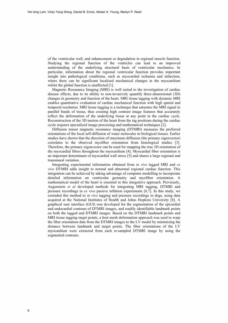
After performing the MR tagging study, the heart was excised and fixed in the end diastolic configuration for collecting DTMRI data (Fig. 2). The procedures are described in [8]. Diffusion tensor data was reconstructed from the diffusion weighted images and the eigenvector associated with maximum diffusion within each voxel was calculated in each DTMRI image. Each image had 256 x 256 in-plane measurements and there were 116 slices. The resolution of the DTMRI data was 390μm x 390μm x 800μm.
Physiological Integration of Structural and Functional Cardiac Magnetic Resonance Imaging Using Finite Element Modelling
7
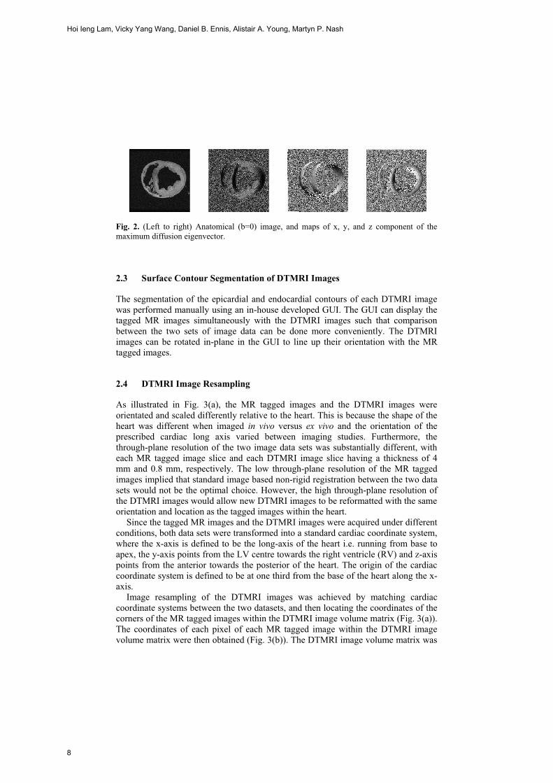
Fig. 2. (Left to right) Anatomical (b=0) image, and maps of x, y, and z component of the maximum diffusion eigenvector.
2.3 Surface Contour Segmentation of DTMRI Images
The segmentation of the epicardial and endocardial contours of each DTMRI image was performed manually using an in-house developed GUI. The GUI can display the tagged MR images simultaneously with the DTMRI images such that comparison between the two sets of image data can be done more conveniently. The DTMRI images can be rotated in-plane in the GUI to line up their orientation with the MR tagged images.
2.4 DTMRI Image Resampling
As illustrated in Fig. 3(a), the MR tagged images and the DTMRI images were orientated and scaled differently relative to the heart. This is because the shape of the heart was different when imaged in vivo versus ex vivo and the orientation of the prescribed cardiac long axis varied between imaging studies. Furthermore, the through-plane resolution of the two image data sets was substantially different, with each MR tagged image slice and each DTMRI image slice having a thickness of 4 mm and 0.8 mm, respectively. The low through-plane resolution of the MR tagged images implied that standard image based non-rigid registration between the two data sets would not be the optimal choice. However, the high through-plane resolution of the DTMRI images would allow new DTMRI images to be reformatted with the same orientation and location as the tagged images within the heart.
Since the tagged MR images and the DTMRI images were acquired under different conditions, both data sets were transformed into a standard cardiac coordinate system, where the x-axis is defined to be the long-axis of the heart i.e. running from base to apex, the y-axis points from the LV centre towards the right ventricle (RV) and z-axis points from the anterior towards the posterior of the heart. The origin of the cardiac coordinate system is defined to be at one third from the base of the heart along the x-axis.
Image resampling of the DTMRI images was achieved by matching cardiac coordinate systems between the two datasets, and then locating the coordinates of the corners of the MR tagged images within the DTMRI image volume matrix (Fig. 3(a)). The coordinates of each pixel of each MR tagged image within the DTMRI image volume matrix were then obtained (Fig. 3(b)). The DTMRI image volume matrix was
Hoi Ieng Lam, Vicky Yang Wang, Daniel B. Ennis, Alistair A. Young, Martyn P. Nash
8
then resampled at the locations of the MR tagged images within the volume, and also at evenly-spaced parallel planes between the MR tagged images (Fig. 3(c)).
(a) (b) (c)
Fig. 3. (a) The DTMRI image slice planes (lines) and the segmented contours of the MR tagged images (markers) plotted in the cardiac coordinate system, showing the misalignment between the two data sets. (b) The slice positions of the MR tagged images transformed into the DTMRI image volume (confined by the box). The DTMRI image volume was resampled at these slice positions of the tagged images. (c) The resampled DTMRI image slice planes (lines) and the contours of MR tagged images (markers) plotted in the cardiac coordinate system.
2.5 Fibre Orientation Data Extraction
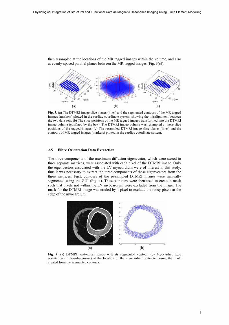
The three components of the maximum diffusion eigenvector, which were stored in three separate matrices, were associated with each pixel of the DTMRI image. Only the eigenvectors associated with the LV myocardium were of interest in this study, thus it was necessary to extract the three components of these eigenvectors from the three matrices. First, contours of the re-sampled DTMRI images were manually segmented using the GUI (Fig. 4). These contours were then used to create a mask such that pixels not within the LV myocardium were excluded from the image. The mask for the DTMRI image was eroded by 1 pixel to exclude the noisy pixels at the edge of the myocardium.
(a) (b)
Fig. 4. (a) DTMRI anatomical image with its segmented contour. (b) Myocardial fibre orientation (in two-dimension) at the location of the myocardium extracted using the mask created from the segmented contours.
Physiological Integration of Structural and Functional Cardiac Magnetic Resonance Imaging Using Finite Element Modelling
9

2.6 Landmark Selection
The GUI described above also allows the selection of fiducial markers (e.g. papillary muscles, RV inserts) on the MR tagged images and the corresponding re-sampled DTMRI images (Fig. 5). For each pair of corresponding MR tagged image and DTMRI resampled image, fiducial markers were first selected from the tagged image and each marker was sequentially assigned a number to indicate the order of selection. Then the same number of fiducial markers was selected on the DTMRI image in the same sequential order. The fiducial markers selected on the MR tagged images were referred to as target points, and those on the DTMRI images were referred to as landmark points and were used for host mesh fitting.
Fig. 5. A screenshot of the GUI showing the manually segmented contours on the DTMRI image (right side), and the manually selected fiducial markers on both the MR tagged image (left side) and DTMRI image.
3 Host Mesh Fiber Mapping
As described above, the segmented contours of the DTMRI images and the tagged MRI images exhibited different orientations in 3D, since the canine heart was imaged during different conditions. Therefore, it is necessary to ensure that the geometry defined by the DTMRI images and the tagged MR images was consistent before the fiber orientation data were incorporated to the finite element geometric model created. This was achieved by performing host mesh fitting, a technique which was designed to customize generic models to specific cases [11]. In our study, we used the host mesh fitting technique to warp the DTMRI data into the in vivo geometric model defined by the tagged MRI data. This host mesh fitting approach involved minimizing the distance between two sets of points: landmark points selected from the resampled
Hoi Ieng Lam, Vicky Yang Wang, Daniel B. Ennis, Alistair A. Young, Martyn P. Nash
10

DTMRI images and corresponding target points selected from the MR tagged images. This minimization was implemented by embedding the landmark points in another finite element mesh, called the host mesh and minimizing the total squared error with respect to host mesh nodal parameters. The host mesh used for this study was a simple tri-cubic mesh consisting of 1 element connected with 8 element nodes (Fig 6). Since the target points were embedded in the host mesh, any deformation the host mesh underwent caused an interpolated degree of deformation for the target points. That is, the local coordinates of the target points with respect to the host mesh remained unchanged before and after deformation. Because the host mesh had a simpler geometry and fewer number of elements, the computational cost of this minimization was reduced significantly, an important benefit of host mesh fitting. Once the optimum host mesh nodal parameters were evaluated, the global coordinates of landmark points were updated based on the local coordinates defined with respect to the host mesh nodal parameters and the transformation matrix obtained during fitting. The same transformation matrix was also applied to the DTMRI data so that the geometries defined by DTMRI and tagged MRI were consistent. Subsequently, fiber orientations could then be embedded into the geometric model using the deformation gradients from the host mesh transformation, and used for mechanical analysis.
(a) (b)
(c) (d)
Fig. 6. (a) Undeformed host mesh (lines) with landmark points (light) and target points (dark). (b) Deformed host mesh with target points and transformed landmark. (c) A through-plane view of the landmark and target points for one slice before host mesh fitting. (d) A through-plane view of the landmark and target points from the same slice after host mesh fitting. The host mesh fit reduced the root mean squared error between landmark and target points from 4.1 mm to 0.8 mm.
Physiological Integration of Structural and Functional Cardiac Magnetic Resonance Imaging Using Finite Element Modelling
11

4 Left Ventricular Finite Element Model
4.1 Left Ventricular Anatomy and Structure
A mathematical model of the LV was created in the cardiac coordinate system based on non-linear finite element optimization of the model geometry to the segmented contours of the MR tagged images (Fig. 7). A regular ellipsoid was initially created in a prolate spheroidal coordinate system, using dimensions based on the base-to-apex dimension and wall thickness estimated from MR tagged images. Prolate spheroidal coordinates were used to define the heart geometry in order to reduce the number of elements needed to represent the complex three-dimensional ventricular geometry. A rectangular Cartesian coordinate system, however, was employed for tissue mechanics analysis. The ellipsoid consisted of 16 finite elements which included 4 circumferential elements, 4 longitudinal elements and 1 transmural element (Fig. 4). A material coordinate system was also defined such that it was attached to material points and moved with the myocardium as it deformed. Finite element material coordinates (�1,�2,�3) were directly associated with element geometry, with �1 in the circumferential direction, �2 in the transmural direction, and �3 in the longitudinal (apex-base) direction. The spatial variation of geometric information within each element was approximated using tri-cubic Hermite interpolation of parameters defined at the element nodes, which implicitly enforces spatial gradient continuity across element boundaries [12]. The nodal parameters obtained after minimization constituted the optimized geometric model.
(a) (b) (c)
Fig. 7. (a) A regular ellipsoid created as the initial estimate of the LV geometric model where x: base-to-apex, y: left-to-right, and z: anterior-to-posterior. (b) Epicardial surface of the initial ellipsoid fitted to the short axis epicardial contour. (c) Endocardial surface of the initial ellipsoid fitted to the short axis endocardial contour. The root mean squared error in the surface fit was 0.8 mm.
The LV fiber architecture can be defined throughout the LV geometry using nonlinear optimization of a fiber field to the transformed fiber vectors derived from DTMRI, using the methods outlined in [7].
Hoi Ieng Lam, Vicky Yang Wang, Daniel B. Ennis, Alistair A. Young, Martyn P. Nash
12
4.2 Left Ventricular Mechanics
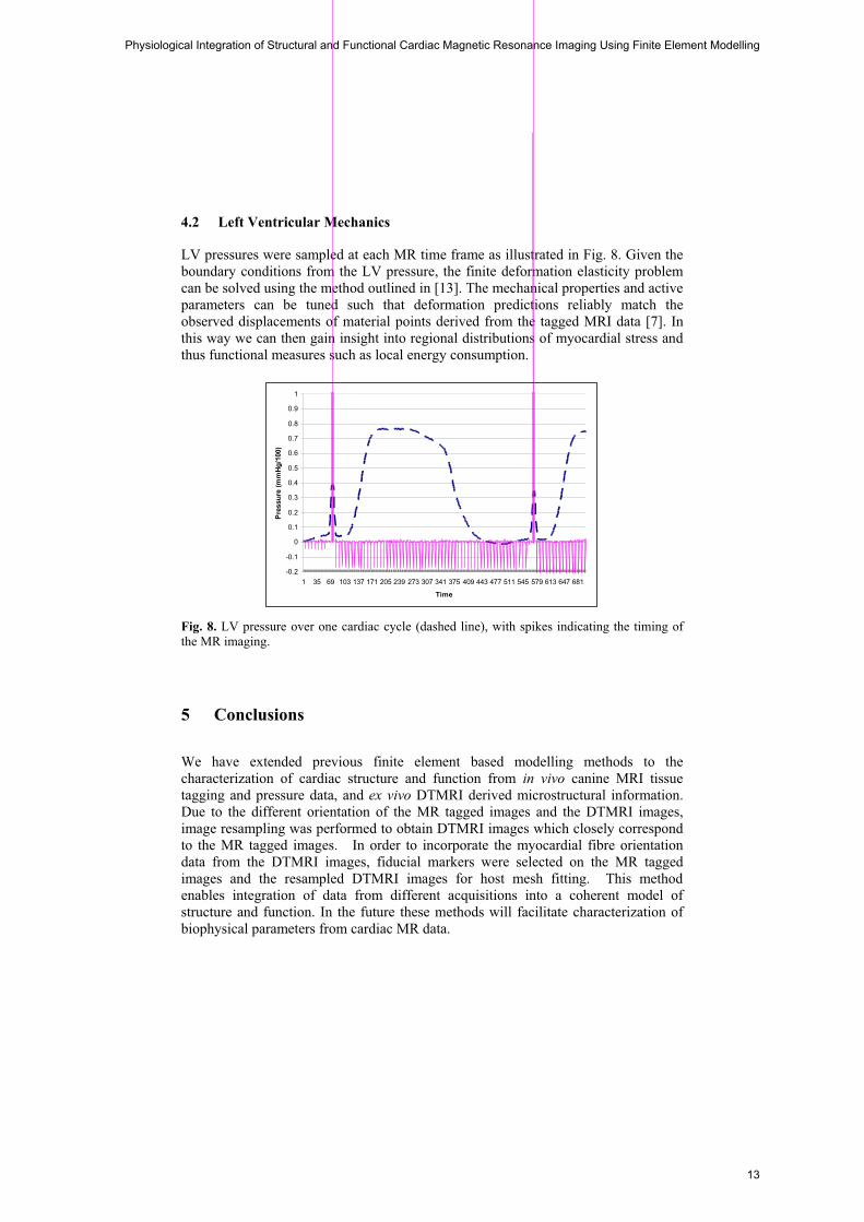
LV pressures were sampled at each MR time frame as illustrated in Fig. 8. Given the boundary conditions from the LV pressure, the finite deformation elasticity problem can be solved using the method outlined in [13]. The mechanical properties and active parameters can be tuned such that deformation predictions reliably match the observed displacements of material points derived from the tagged MRI data [7]. In this way we can then gain insight into regional distributions of myocardial stress and thus functional measures such as local energy consumption.
-0.2
-0.1
0
0.1
0.2
0.3
0.4
0.5
0.6
0.7
0.8
0.9
1
1 35 69 103 137 171 205 239 273 307 341 375 409 443 477 511 545 579 613 647 681
Time
Pres
sure
(mm
Hg/1
00)
Fig. 8. LV pressure over one cardiac cycle (dashed line), with spikes indicating the timing of the MR imaging.
5 Conclusions
We have extended previous finite element based modelling methods to the characterization of cardiac structure and function from in vivo canine MRI tissue tagging and pressure data, and ex vivo DTMRI derived microstructural information. Due to the different orientation of the MR tagged images and the DTMRI images, image resampling was performed to obtain DTMRI images which closely correspond to the MR tagged images. In order to incorporate the myocardial fibre orientation data from the DTMRI images, fiducial markers were selected on the MR tagged images and the resampled DTMRI images for host mesh fitting. This method enables integration of data from different acquisitions into a coherent model of structure and function. In the future these methods will facilitate characterization of biophysical parameters from cardiac MR data.
Physiological Integration of Structural and Functional Cardiac Magnetic Resonance Imaging Using Finite Element Modelling
13
References
1. Glass, L., Hunter, P. and McCulloch, A. (eds.): Theory of heart: biomechanics, biophysics,
and nonlinear dynamics of cardiac function. Springer-Verlag, New York (1991) 2. O’Dell, W.G., Moore, C.C., Hunter, W.C., Zerhouni, E.A., McVeigh, E.R.: Three-
dimensional Myocardial Deformations: Calculation with Displacement Field Fitting to Tagged MR Images. Radiology 195 (1995) 829-835
3. Le Bihan, D., Mangin, J.F., Poupon, C., Clark, C.A., Pappata, S., Molko, N., Chabriat, H.: Diffusion Tensor Imaging: Concepts and Applications. Journal of Magnetic Resonance Imaging 13 (2001) 534-546
4. Douek, P., Turner, R., Pekar, J., Patronas N. J., Le Bihan, D.: MR color mapping of myelin fiber orientation. Journal of Computer Assisted Tomography 15 (1991) 923-929
5. Geerts, L., Bovendeerd, P., Nicolay, K., Arts, T.: Characterization of the normal cardiac myofiber field in goat measured with MR-diffusion tensor imaging. American Journal of Physiology (Heart and Circulatory Physiology) 283 (2002) H139-H145
6. Augenstein, K.F., Cowan, B.R., LeGrice, I.J., Young, A.A.: Estimation of cardiac hyperelastic material properties from MRI tissue tagging and diffusion tensor imaging. MICCAI 9:1 (2006) 628-635
7. Augenstein, K.F., Cowan, B.R., LeGrice, I.J., Nielsen, P.M., Young, A.A.: Method and apparatus for soft tissue material parameter estimation using tissue tagged Magnetic Resonance Imaging. J Biomech Eng. 127:1 (2005) 148-157
8. Ennis, D.B.: Assessment of Myocardial Structure and Function Using Magnetic Resonance Imaging. PhD Thesis, John Hopkins University (2004). (See also http://www.ccbm.jhu.edu)
9. Guttman, M.A., Prince, J.L., McVeigh, E.R.: Tag and contour detection in tagged MR images of the left ventricle. IEEE Trans. Med. Imaging 13 (1997) 74-88
10. Ozturk, C., McVeigh, E.R..: Four dimensional B-Spline based motion analysis of tagged MR Images: introduction and in-vivo validation. Phys. Med. Bio. 45 (2000) 1683-1702
11. LeGrice, I., Hunter, P.J., Young, A.A., Smaill, B.: The architecture of the heart: a data-based model. Phil. Trans. R. Soc. Lond. 359 (2001) 1217-1232
12. Bradley, C.P., Pullan, A.J., Hunter, P.J.: Geometric Modeling of the Human Torso Using Cubic Hermite Elements. Annals of Biomedical Engineering 25 (1997) 96-111
13. Nash, M.P., Hunter, P.J.: Computational Mechanics of the Heart: From Tissue Structure to Ventricular Function. Journal of Elasticity 61 (2000) 113-141
Hoi Ieng Lam, Vicky Yang Wang, Daniel B. Ennis, Alistair A. Young, Martyn P. Nash
14
Meshless Methods for LV Strain Computationsfrom Tagged MRI
Suejung Huh1, Xiaoxu Wang1, Dimitis Metaxas1, and Leon Axel2
1 Rutgers University, Piscataway NJ, 08854, [email protected],
2 New York University, 660 First Avenue, New York, NY, 10016, USA
Abstract. This paper presents a meshless framework to compute strainin the left ventricle from Tagged MRI. Our meshless framework allowsthe computation of a complex but smooth strain field, since it is notbounded to the underlying mesh structure of a model. In this paper,we used Tagged MR images of left ventricles. However, the suggestedformulation is independent of the image modality and the choice of fittingmechanism.
1 Introduction
A meshless method to solve partial differential equations was introduced in com-putational mechanics by [1] according to [2], although the meshless method itselfwas introduced in the 70’s [3]. Despite their great flexibility, meshless methodshave not been utilized significantly in the medical field. Recently the meshlessapproach was utilized to model surgical processes [4, 5]. Meshless approachesare well suited to model a biomedical organ in surgical simulations, when thetopology of the organ changes interactively by surgical processes such as cut-ting and stitching. The fundamental flexibility of the meshless approach lies inthe following : 1) a field is defined by the not-explicitly-connected participatingparticles, 2) we can change the density of the constitutive particle populationswithout changing the field property, and 3) any changes in such constitutive par-ticles can be handled locally. Since a meshless approach has such flexibility, it isappropriate for strain computations, in areas where we observe drastic changesin deformation patterns.
The left ventricle (LV) exhibits large deformations during the cardiac cycle[2],and has a very complex geometry with varying material properties in the en-docardium [6]. Galerkin approaches on discretized domains, such as like FiniteElement Methods (FEM) or Boundary Element Methods (BEM), have been usedin numerous studies of strain analysis of LV deformations, including [7–12]. How-ever, when we compute strains during the LV deformation, spatially discretizedelements like the ones used in FEM or BEM could be too coarse to encompass allthe details of the strain field. Furthermore, increasing the number of volumetricelements to express all the details could be computationally expensive, and moreimportantly erroneous, since it could produce too many degenerate volumetric
15
elements during a simulation. Having such irregularly shaped elements could un-dermine the stability of simulations. Hence we introduce a meshless formulationto compute the strain field for LV during systole.
In Sec. 2, we introduce our meshless strain formulation method, and in Sec.3, the methodology for fitting is explained. Sec. 4 shows the experimental resultstested on two slices of the in-vivo myocardium, and a discussion with futuredirections follows in Sec. 5.
2 Meshless Strain Computation
In order to measure the deformation of the LV, strain fields of the LV havebeen analyzed by many researchers. In this paper, we measure the strain fieldusing the meshless method. In the meshless method, an object is representedby points only. All points are not explicitly connected. The strain tensor of apoint is computed based on the neighboring points. Obtained strain fields willbe smooth because all the strain tensors are based on their neighbors. Amongseveral ways to compute strain [13], we use the lagrangian strain tensor since itis more suitable for large deformations and reports deformations with respect tothe original shape of an object.
2.1 Strain Computation for Large deformations
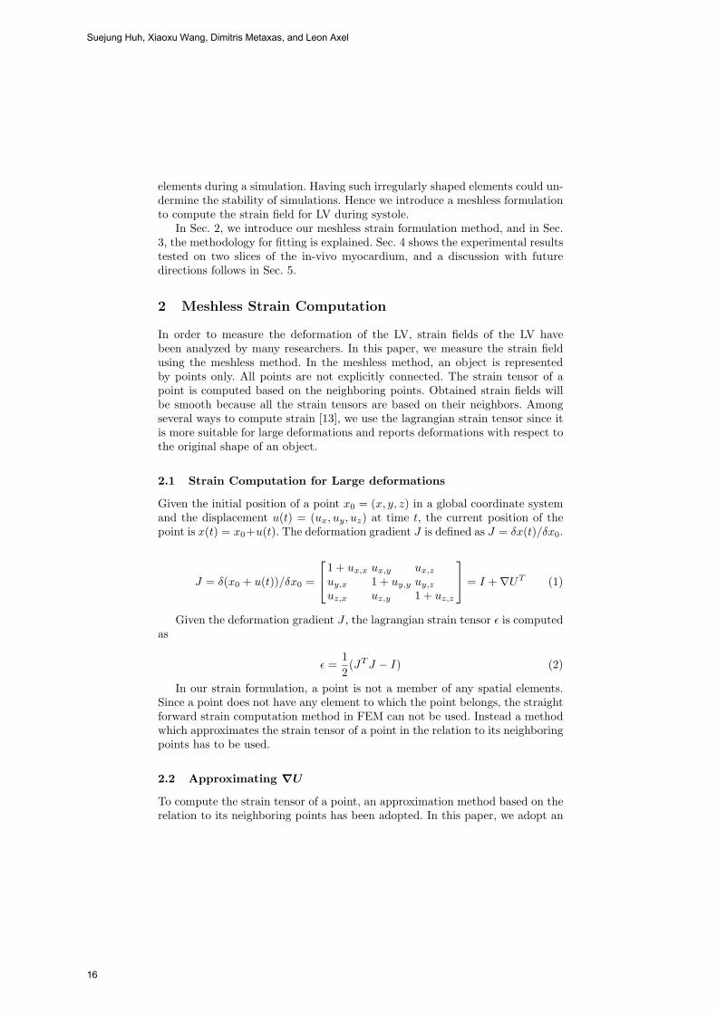
Given the initial position of a point x0 = (x, y, z) in a global coordinate systemand the displacement u(t) = (ux, uy, uz) at time t, the current position of thepoint is x(t) = x0+u(t). The deformation gradient J is defined as J = δx(t)/δx0.
J = δ(x0 + u(t))/δx0 =
⎡⎣1 + ux,x ux,y ux,zuy,x 1 + uy,y uy,zuz,x uz,y 1 + uz,z
⎤⎦ = I + ∇UT (1)
Given the deformation gradient J , the lagrangian strain tensor ε is computedas
ε =12(JTJ − I) (2)
In our strain formulation, a point is not a member of any spatial elements.Since a point does not have any element to which the point belongs, the straightforward strain computation method in FEM can not be used. Instead a methodwhich approximates the strain tensor of a point in the relation to its neighboringpoints has to be used.
2.2 Approximating ∇U
To compute the strain tensor of a point, an approximation method based on therelation to its neighboring points has been adopted. In this paper, we adopt an
Suejung Huh, Xiaoxu Wang, Dimitris Metaxas, and Leon Axel
16
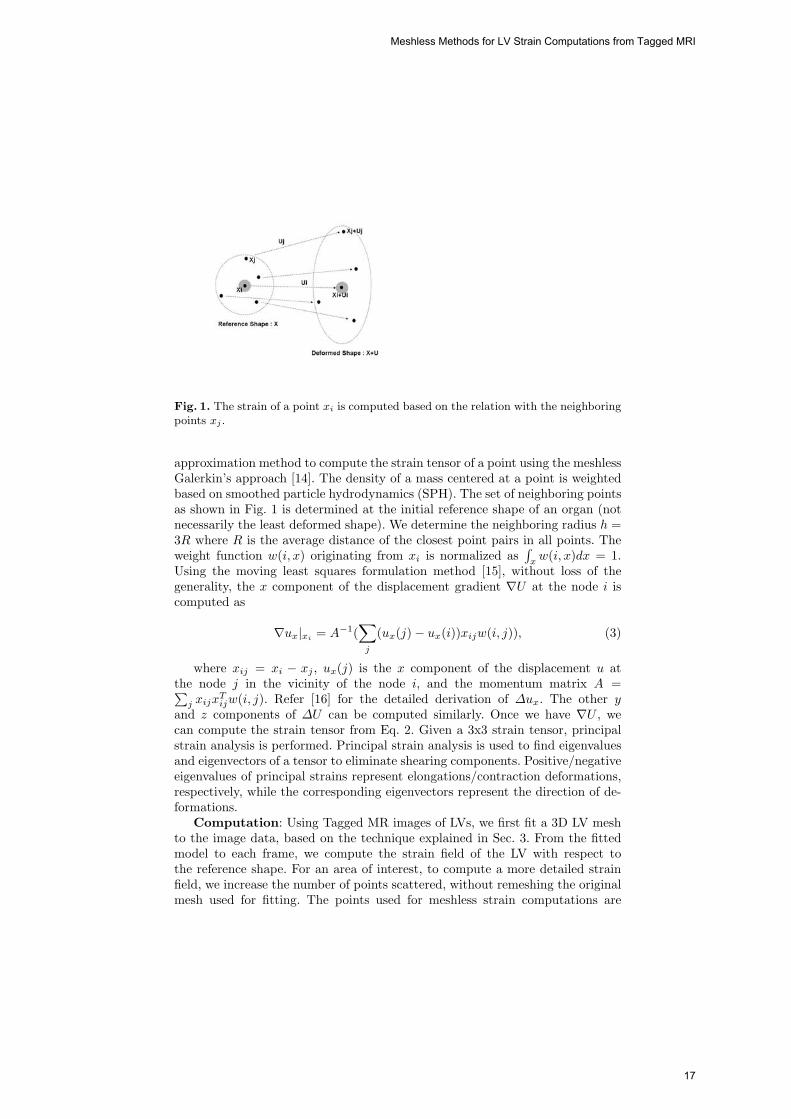
Fig. 1. The strain of a point xi is computed based on the relation with the neighboringpoints xj .
approximation method to compute the strain tensor of a point using the meshlessGalerkin’s approach [14]. The density of a mass centered at a point is weightedbased on smoothed particle hydrodynamics (SPH). The set of neighboring pointsas shown in Fig. 1 is determined at the initial reference shape of an organ (notnecessarily the least deformed shape). We determine the neighboring radius h =3R where R is the average distance of the closest point pairs in all points. Theweight function w(i, x) originating from xi is normalized as
∫xw(i, x)dx = 1.
Using the moving least squares formulation method [15], without loss of thegenerality, the x component of the displacement gradient ∇U at the node i iscomputed as
∇ux|xi = A−1(∑j
(ux(j) − ux(i))xijw(i, j)), (3)
where xij = xi − xj , ux(j) is the x component of the displacement u atthe node j in the vicinity of the node i, and the momentum matrix A =∑
j xijxTijw(i, j). Refer [16] for the detailed derivation of Δux. The other y
and z components of ΔU can be computed similarly. Once we have ∇U , wecan compute the strain tensor from Eq. 2. Given a 3x3 strain tensor, principalstrain analysis is performed. Principal strain analysis is used to find eigenvaluesand eigenvectors of a tensor to eliminate shearing components. Positive/negativeeigenvalues of principal strains represent elongations/contraction deformations,respectively, while the corresponding eigenvectors represent the direction of de-formations.
Computation: Using Tagged MR images of LVs, we first fit a 3D LV meshto the image data, based on the technique explained in Sec. 3. From the fittedmodel to each frame, we compute the strain field of the LV with respect tothe reference shape. For an area of interest, to compute a more detailed strainfield, we increase the number of points scattered, without remeshing the originalmesh used for fitting. The points used for meshless strain computations are
Meshless Methods for LV Strain Computations from Tagged MRI
17
defined based on their barycentric coordinates with respect to the underlyingmesh structure. Thus more points can be added for strain estimation after thefitting.
2.3 Comparison with FEM
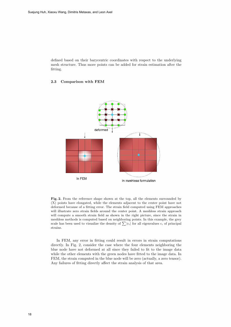
Fig. 2. From the reference shape shown at the top, all the elements surrounded by(X) points have elongated, while the elements adjacent to the center point have notdeformed because of a fitting error. The strain field computed using FEM approacheswill illustrate zero strain fields around the center point. A meshless strain approachwill compute a smooth strain field as shown in the right picture, since the strain inmeshless methods is computed based on neighboring points. In this example, the greyscale has been used to visualize the density of
∑ |εi| for all eigenvalues εi of principalstrains.
In FEM, any error in fitting could result in errors in strain computationsdirectly. In Fig. 2, consider the case where the four elements neighboring theblue node have not deformed at all since they failed to fit to the image datawhile the other elements with the green nodes have fitted to the image data. InFEM, the strain computed in the blue node will be zero (actually, a zero tensor).Any failures of fitting directly affect the strain analysis of that area.
Suejung Huh, Xiaoxu Wang, Dimitris Metaxas, and Leon Axel
18
In meshless formulation, this adverse effect of a fitting failure can be mini-mized, provided the vicinity of the center node includes more neighboring nodesother than (x) marked nodes, since the strain field is computed in conjunctionwith all its neighboring nodes (Extended kernel). Although the volume definedby the (x) marked nodes and the center node have not deformed at all, the strainfield on the center node still could be a smooth tensor as it is influenced by othergreen nodes. Hence a small fitting error does not affect the strain analysis di-rectly. For the case, where we actually expect a small scale of deformations, wecan populate the area with more nodes with a smaller vicinity threshold to cap-ture small details. Expanding the kernel size of the meshless approach excessivelywill smoothen the strain field unnecessarily. Picking the appropriate kernel sizefor each application is essential to maintain the correctness of the system.
3 LV Fitting
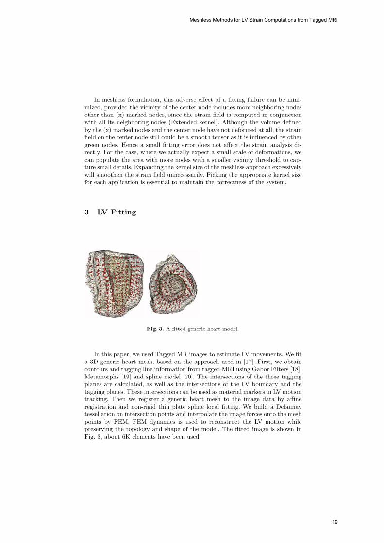
Fig. 3. A fitted generic heart model
In this paper, we used Tagged MR images to estimate LV movements. We fita 3D generic heart mesh, based on the approach used in [17]. First, we obtaincontours and tagging line information from tagged MRI using Gabor Filters [18],Metamorphs [19] and spline model [20]. The intersections of the three taggingplanes are calculated, as well as the intersections of the LV boundary and thetagging planes. These intersections can be used as material markers in LV motiontracking. Then we register a generic heart mesh to the image data by affineregistration and non-rigid thin plate spline local fitting. We build a Delaunaytessellation on intersection points and interpolate the image forces onto the meshpoints by FEM. FEM dynamics is used to reconstruct the LV motion whilepreserving the topology and shape of the model. The fitted image is shown inFig. 3, about 6K elements have been used.
Meshless Methods for LV Strain Computations from Tagged MRI
19

Fig. 4. The strain field from a slice in the middle of LV, visualized in different eigen-vectors. The middle slice is shown in the left most picture. The strain elements ofinterest are visualized in 3D and the images are taken from the top view. Circumfer-ential Strain(Contraction): The upper pictures show the contraction deformation ofthe LV. Each edge represents the eigenvector corresponding to the negative eigenvalueof the principal strains. The length of each eigenvector is determined by its eigen-value. Radial Strain(Elongation): Lower Pictures show the elongation deformationof LV. Each edge represents the eigenvector corresponding to the largest positive eigen-value of the principal strains, whose length is determined by its eigenvalue. IncreasedPoints:In both type of deformations, the right pictures show results with more popu-lated point cloud.
Fig. 5. All the eigenvalues from ten subjects were plotted with respect to the pointsused in the meshless method. Left(Elongation): The largest positive eigenvalues.Center(Contraction): The largest magnitude least negative eigenvalues. Right: Thethird principal (smallest magnitude) eigenvalues.
Suejung Huh, Xiaoxu Wang, Dimitris Metaxas, and Leon Axel
20
4 Results
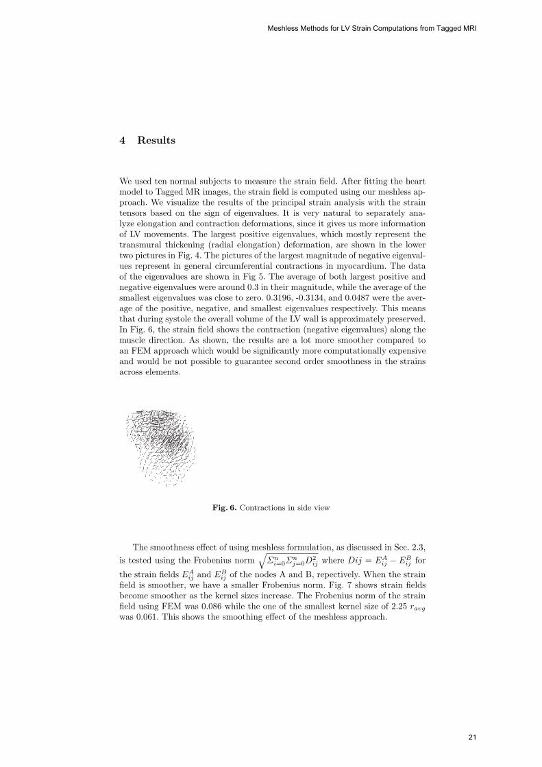
We used ten normal subjects to measure the strain field. After fitting the heartmodel to Tagged MR images, the strain field is computed using our meshless ap-proach. We visualize the results of the principal strain analysis with the straintensors based on the sign of eigenvalues. It is very natural to separately ana-lyze elongation and contraction deformations, since it gives us more informationof LV movements. The largest positive eigenvalues, which mostly represent thetransmural thickening (radial elongation) deformation, are shown in the lowertwo pictures in Fig. 4. The pictures of the largest magnitude of negative eigenval-ues represent in general circumferential contractions in myocardium. The dataof the eigenvalues are shown in Fig 5. The average of both largest positive andnegative eigenvalues were around 0.3 in their magnitude, while the average of thesmallest eigenvalues was close to zero. 0.3196, -0.3134, and 0.0487 were the aver-age of the positive, negative, and smallest eigenvalues respectively. This meansthat during systole the overall volume of the LV wall is approximately preserved.In Fig. 6, the strain field shows the contraction (negative eigenvalues) along themuscle direction. As shown, the results are a lot more smoother compared toan FEM approach which would be significantly more computationally expensiveand would be not possible to guarantee second order smoothness in the strainsacross elements.
Fig. 6. Contractions in side view
The smoothness effect of using meshless formulation, as discussed in Sec. 2.3,is tested using the Frobenius norm
√Σni=0Σ
nj=0D
2ij where Dij = EA
ij − EBij for
the strain fields EAij and EB
ij of the nodes A and B, repectively. When the strainfield is smoother, we have a smaller Frobenius norm. Fig. 7 shows strain fieldsbecome smoother as the kernel sizes increase. The Frobenius norm of the strainfield using FEM was 0.086 while the one of the smallest kernel size of 2.25 ravgwas 0.061. This shows the smoothing effect of the meshless approach.
Meshless Methods for LV Strain Computations from Tagged MRI
21
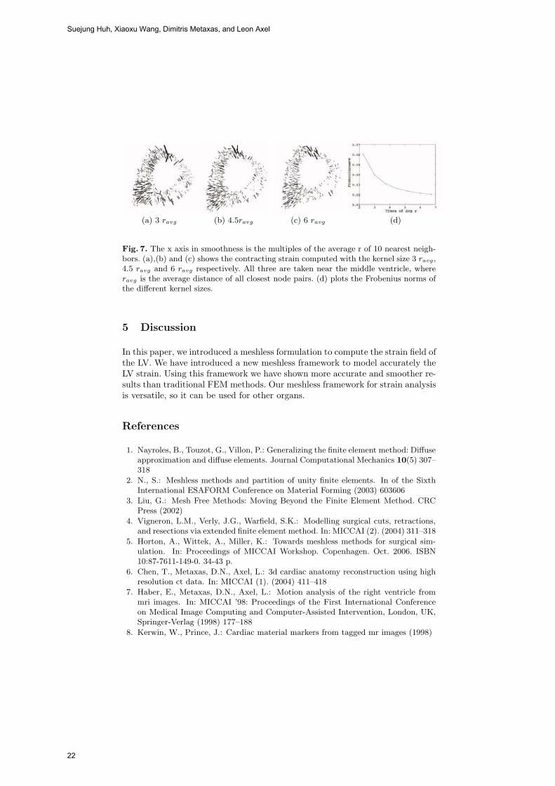
(a) 3 ravg (b) 4.5ravg (c) 6 ravg (d)
Fig. 7. The x axis in smoothness is the multiples of the average r of 10 nearest neigh-bors. (a),(b) and (c) shows the contracting strain computed with the kernel size 3 ravg,4.5 ravg and 6 ravg respectively. All three are taken near the middle ventricle, whereravg is the average distance of all closest node pairs. (d) plots the Frobenius norms ofthe different kernel sizes.
5 Discussion
In this paper, we introduced a meshless formulation to compute the strain field ofthe LV. We have introduced a new meshless framework to model accurately theLV strain. Using this framework we have shown more accurate and smoother re-sults than traditional FEM methods. Our meshless framework for strain analysisis versatile, so it can be used for other organs.
References
1. Nayroles, B., Touzot, G., Villon, P.: Generalizing the finite element method: Diffuseapproximation and diffuse elements. Journal Computational Mechanics 10(5) 307–318
2. N., S.: Meshless methods and partition of unity finite elements. In of the SixthInternational ESAFORM Conference on Material Forming (2003) 603606
3. Liu, G.: Mesh Free Methods: Moving Beyond the Finite Element Method. CRCPress (2002)
4. Vigneron, L.M., Verly, J.G., Warfield, S.K.: Modelling surgical cuts, retractions,and resections via extended finite element method. In: MICCAI (2). (2004) 311–318
5. Horton, A., Wittek, A., Miller, K.: Towards meshless methods for surgical sim-ulation. In: Proceedings of MICCAI Workshop. Copenhagen. Oct. 2006. ISBN10:87-7611-149-0. 34-43 p.
6. Chen, T., Metaxas, D.N., Axel, L.: 3d cardiac anatomy reconstruction using highresolution ct data. In: MICCAI (1). (2004) 411–418
7. Haber, E., Metaxas, D.N., Axel, L.: Motion analysis of the right ventricle frommri images. In: MICCAI ’98: Proceedings of the First International Conferenceon Medical Image Computing and Computer-Assisted Intervention, London, UK,Springer-Verlag (1998) 177–188
8. Kerwin, W., Prince, J.: Cardiac material markers from tagged mr images (1998)
Suejung Huh, Xiaoxu Wang, Dimitris Metaxas, and Leon Axel
22

9. Shi, P., Sinusas, A.J., Constable, R.T., Duncan, J.S.: Volumetric deformation anal-ysis using mechanics-based data fusion: Applications in cardiac motion recovery.Int. J. Comput. Vision 35(1) (1999) 87–107
10. Hu, Z., Metaxas, D.N., Axel, L.: In-vivo strain and stress estimation of the leftventricle from mri images. In: MICCAI ’02: Proceedings of the 5th InternationalConference on Medical Image Computing and Computer-Assisted Intervention-Part I, London, UK, Springer-Verlag (2002) 706–713
11. Park, K., Metaxas, D.N., Axel, L.: A finite element model for functional analysisof 4d cardiac-tagged mr images. In: MICCAI (1). (2003) 491–498
12. Yan, P., Lin, N., Sinusas, A.J., Duncan, J.S.: A boundary element-based approachto analysis of lv deformation. In: MICCAI. (2005) 778–785
13. Fung, Y.C.: A first course in continuum mechanics. Prentice-Hall (1969)14. Belytschko, T., Krongauz, Y., Organ, D., Fleming, M.: Meshless methods : An
overview and recent developments. Civil and Mechanical Engineering, Northwest-ern University (1996)
15. P., L., K., S.: Surfaces generated by moving least squares methods. Mathematicsof Computation 87 (1981) 141–158
16. Muller, M., Keiser, R., Nealen, A., Pauly, M., Gross, M., Alexa, M.: Point basedanimation of elastic, plastic and melting objects. In: SCA ’04: Proceedings of the2004 ACM SIGGRAPH/Eurographics symposium on Computer animation, Aire-la-Ville, Switzerland, Switzerland, Eurographics Association (2004) 141–151
17. Wang, X., Schaerer, J., Qian, Z., Metaxas, D., Chen, T., Axel, L.: Reconstructionof detailed left ventricle motion using deformable model from tagged mrimage
18. Qian, Z., Metaxas, D.N., Axel, L.: Extraction and tracking of MRI tagging sheetsusing a 3D gabor filter bank. Proceedings of Intl Conf. of the Engineering inMedicine and Biology Society (2006)
19. Huang, X., Metaxas, D., Chen, T.: Metamorphs: Deformable shape and texturemodels xiaolei huang metaxas, d. ting chen. Computer Vision and Pattern Recog-nition, 2004. (2004)
20. Axel, L., Chen, T., Manglik, T.: Dense myocardium deformation estimation for 2dTagged MRI. In: FIMH. (2005) 446–456
Meshless Methods for LV Strain Computations from Tagged MRI
23
PPU-based deformable models for
Catheterisation Training
Jixiang Guo1, Shun Li1, Yim Pan Chui1, Qiang Meng1, Howard Zhang1,Simon Chun Ho Yu2, Pheng Ann Heng1,3
1Department of Computer Science and Engineering,The Chinese University of Hong Kong, Shatin, Hong Kong2Department of Diagnostic Radiology and Organ Imaging,The Chinese University of Hong Kong, Shatin, Hong Kong
3Shun Hing Institute of Advanced Engineering,The Chinese University of Hong Kong, Shatin, Hong Kong
Abstract. In this paper, we propose a framework for generating de-formable models for catheterisation training applications. Through ex-ploiting centreline extraction, graph reconstruction, curve fitting andcurve framing techniques, we can model vascular structures and othervirtual catheterisation devices using mathematically contrived geome-tries with minimal user interactions. A Physics Processing Unit (PPU)based incremental voigt model has been proposed for incorporating non-linear biomechanical/mechanical properties into the deformable models.Experiments have shown a reasonable increase in frame rates from 2-foldto 4-fold over non-PPU-based simulations. Our results have demonstatedthe feasility of using this newly evolved multi-core physics acceleratorfor speeding up medical training applications such as virtual vascularcatheterisation.
1 Introduction
Catheterisation has been one of the major medical procedures being used in vas-cular interventional radiology for the remedy of stenosis, aneurysm, etc. Based onimage-guided X-ray fluoroscopy or ultrasonography, a thin flexible tube calledcatheter is inserted into a vessel for vascular procedures such as angiography,angioplasty and embolization. Due to the limited visual perception during theimage-guided procedures, training of these procedures is difficult. Recently, vir-tual reality (VR) based medical simulations have become more popular due totheir reusability and flexibility.
Within a virtual simulation environment for vascular intervention procedures,virtual devices such as guide wires or catheters can often be interacted with eachother. Thus, effective collision computation between various deformable modelsis an essential task. Currently, real-time simulation of deformable models inmedical simulation remains a challenging task. Futhermore, visualizations ofthese procedrues that are of high quality and high fidelity demands even moreintensive computation.
24

2
In this paper, a novel deformable modeling framework for virtual catheteri-sation is proposed. The new personal computer (PC) grade, multicore processorcalled the Physics Processing Unit (PPU) has been exploited in developing ourframework for reconstructing deformable models suitable for interactive medicalsimulations. Vascular structure and virtual devices can be built through an au-tomated topological geometric modeling engine. PPU provides built-in supportof a mass-spring-damper model for describing linear elastic motions. We extendthe model to an incremental-voigt one for simulating the non-linear biomechan-ical stress-strain behaviour of soft tissue. With such an hardware-acceleration,real-time interactivity can be achieved.
2 Related Work
VR based medical simulations for minimally invasive surgery (MIS) has becomemore prevalent in the recent decade. Virtual endoscopy has been exploited tosimulate colonscopy [8], arthroscopy [6], laparoscopy [3] and hysterscopy [5] etc.Developing simulation systems for vascular interventional procedures have beena very active research area [7][2][14]. Many existing works focus on the geometricmodeling of vascular structure for catheter navigation. Nowinski et al. proposeda virtual environment for simulating deformable vascular modeling [11], whereby assuming a static external vessel wall structure, interactive performance canbe achieved. In order to further enhance the realism of the simulation, a moreflexible deformable modeling for vascular structure is needed. In light of this, wepropose the PPU-based framework for modeling and simulating realistic biome-chanical features of the vascular system so that deformable models can be usedfor virtual catheterisation.
3 Modeling Framework
In catheterisation procedures, guide wire or catheter is directed to the regionof interest through blood vessels. Simulated vessel models, and virtual devicesconstitute the basic components of a virtual catheterisation simulation. Basedon angiographic data such as magnetic resonance angiography (MRA) or com-puted tomographic angiography (CTA), centrelines or namely skeletons of theinterested vessels are extracted. An automated topological reconstruction pro-cess is carried out in order to build a geometric model of the vessel. Virtualdevices such as guide wires or catheters can also be built through the modelingframework.
3.1 Skeleton Extraction
The extraction of a vascular skeleton can be done by a two pass procedure. First,a thinning process is performed to locate the skeleton voxels, which represent theabstract vessel information, within a 3D volume of angiographic data. We adopta fully automatic centerline calculation algorithm based on a 3D topologicalthinning proposed in [15]. Then a vessel graph can be constructed.
PPU-based deformable models for Catheterisation training
25
3
3.2 Vessel Graph Construction
Based on the extracted skeleton points, a graph is constructed for later topo-logical reconstruction process. We can consider the structure of the blood vesselas a directed graph. An adjacency list is deployed for such representation wherecenterline points are restored in a linked link. A junction is represented as avertex which has several edges linking to others. The rest of the vertices are re-garded as segment points. Adjacent points with no junction should be arrangedsequentially, the line ends when a junction or end point is found.
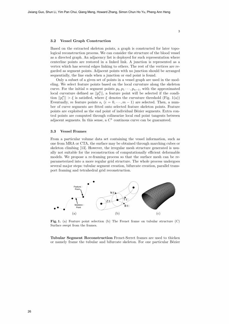
Only a subset of a given set of points in a vessel graph are used in the mod-eling. We select feature points based on the local curvature along the skeletoncurve. For the initial n segment points p0, p1 · · · , pn−1, with the approximatedlocal curvature defined as ||p′′i ||, a feature point will be selected if the condi-tion ||p′′i || > ξ is satisfied, where ξ denotes the curvature threshold (Fig. 1(a))Eventually, m feature points si (i = 0, · · · ,m − 1) are selected. Then, a num-ber of curve segments are fitted onto selected feature skeleton points. Featurepoints are exploited as the end point of individual Bezier segments. Extra con-trol points are computed through colinearize local end point tangents betweenadjacent segments. In this sense, a C1 continous curve can be guaranteed.
3.3 Vessel Frames
From a particular volume data set containing the vessel information, such asone from MRA or CTA, the surface may be obtained through marching cubes orskeleton climbing [13]. However, the irregular mesh structure generated is usu-ally not suitable for the reconstruction of computationally efficient deformablemodels. We propose a re-framing process so that the surface mesh can be re-parameterized into a more regular grid structure. The whole process undergoesseveral major steps: tubular segment creation, bifurcate creation, parallel trans-port framing and tetrahedral grid reconstruction.
�����������
���������� ����
����
����
����
(a) (b) (c)
Fig. 1. (a) Feature point selection (b) The Frenet frame on tubular structure (C)Surface swept from the frames.
Tubular Segment Reconstruction Frenet-Serret frames are used to thickenor namely frame the tubular and bifurcate skeleton. For one particular Bezier
Jixiang Guo, Shun Li, Yim Pan Chui, Qiang Meng, Howard Zhang, Simon Chun Ho Yu, Pheng Ann Heng
26
4
segment Zi(t) t ∈ [0, 1] (Fig. 1(b)), the unit tangent Ti(t), unit normal Ni(t)and unit bi-normal Bi(t) are given by:
Ti(t) =Z′i(t)
||Z′i(t)||
, Bi(t) =Z′i(t)× Z′′
i (t)
||Z′i(t)× Z′′
i (t)|| , and Ni(t) = Bi(t)× Ti(t), t ∈ [0, 1]
One common problem occuring in Frenet framing is that in some cases, thebinormal is not varying smoothly or well-defined at a singular point, e.g. whenthe curve is locally straight. We adopt a correction method which deploys amodified version of parallel transport [1] to tackle these singularities. The mainpurpose of parallel transport is to ensure one particular reference frame (a set oftangent T , normal N and binormal B) is transported as parallel to the previousframe as possible. This method can resolve singularities regardless of the localcurvature throughout the curve. A numerial method for computing the frameis used. For two consecutive tangents, the axis perpendicular to both of themis used as the rotation axis. In this sense, the frame fi+1 can be computed byrotating the previous frame fi by the angle between the two tangents.
After all frames have been computed and corrected, we can generate a seriesof rings for final surface sweeping:
Fi(t, θ) = Bi(t) + r(t)(cosθNi(t) + sinθBi(t)), t ∈ [0, 1], θ ∈ [0, 2π],
where r(t) denotes the radius of the tubular or bifurcate frame. r(t) can bedetermined from the original patient data. Fig. 1(c) shows the resultant surface-swept curve.
Bifurcation Reconstruction Bifurcation framing has to be handled sepa-rately. First, we reconstruct three Bezier segments based on the bifurcate point,C0, and the radius of three tubular segments r1, r2, and r3, respectively. Thesegment end points and the internal control points can be calculated by:
C11 = C0 + r1/2, C12 = C0 + r1;
C21 = C0 + r2/2, C22 = C0 + r2;
C31 = C0 + r3/2, C32 = C0 + r3;
Fig. 2 shows the creation of three bifurcate Bezier segments based on the bifur-cate point. Then, the thickening of these segments can be done by sweeping threehalf tubular surfaces and re-triangulating the inner Bezier triangle. Figs. 3(a)shows an example of tubular grid structure. Fig. 3(b) shows a composite struc-ture.
Tetrahedral Model Based on the geometric model, a dual-layered tetrahedralmass-spring model can be built. The outer layer is the grid-based surface mesh.The inner layer is generated by shooting rays from the centroid of every triangle(of vertices vij , where j = 0, 1, 2) towards its facet normal Ni until the layerdepth has been reached. One bottom vertex is corresponding to one upper trian-gle. The position of this bottom vertex bi can be given by bi = vi0+vi1+vi2
3 +Nil,where l denotes the layer depth. We can then attach each triangle vertex to
PPU-based deformable models for Catheterisation training
27
5
��
���������
���
���
���
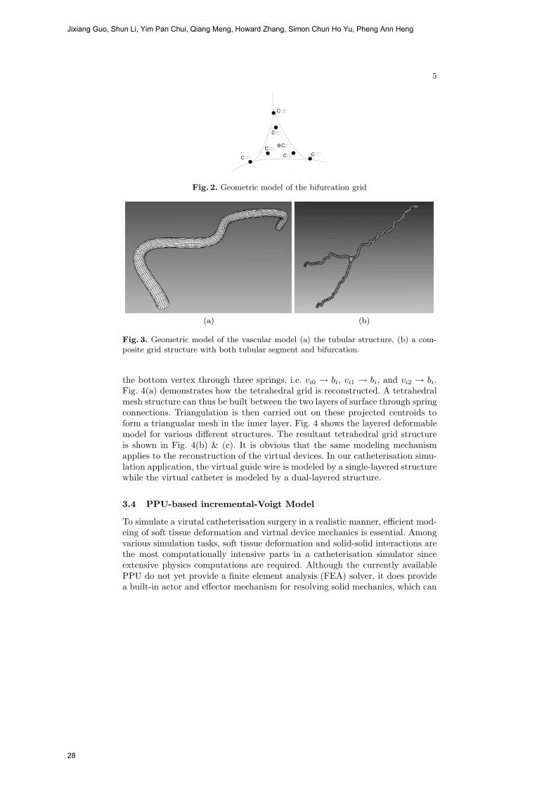
Fig. 2. Geometric model of the bifurcation grid
(a) (b)
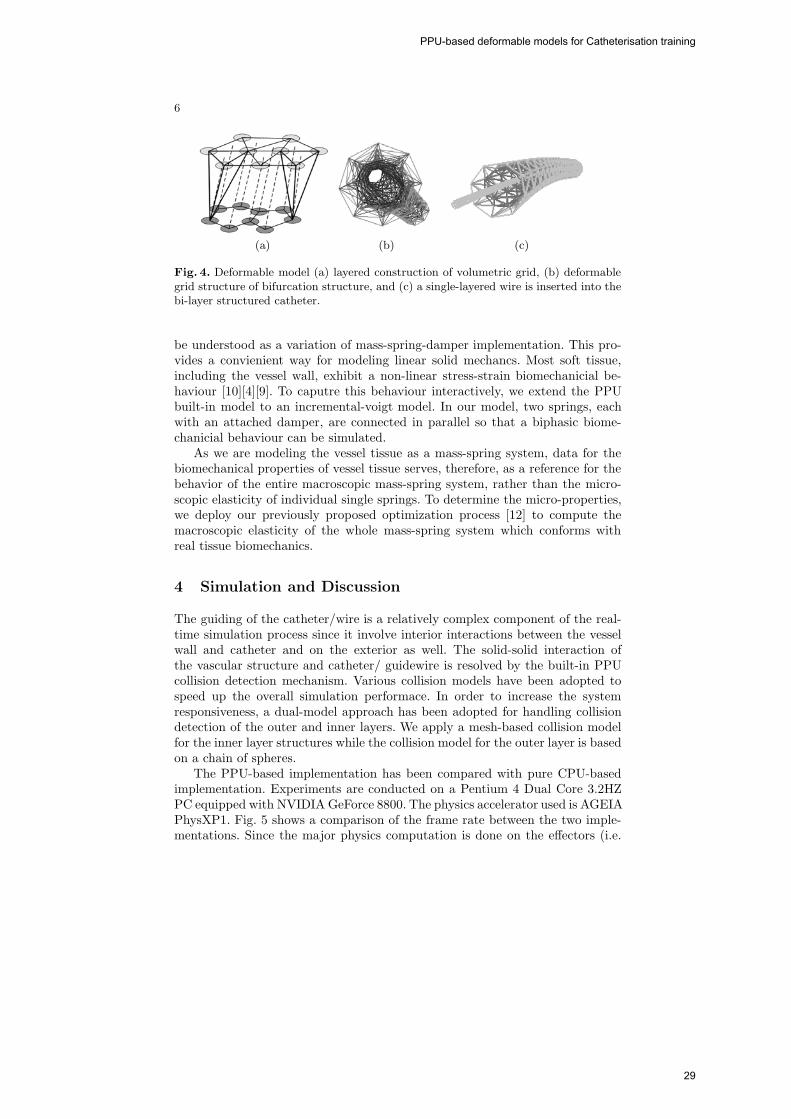
Fig. 3. Geometric model of the vascular model (a) the tubular structure, (b) a com-posite grid structure with both tubular segment and bifurcation.
the bottom vertex through three springs, i.e. vi0 → bi, vi1 → bi, and vi2 → bi.Fig. 4(a) demonstrates how the tetrahedral grid is reconstructed. A tetrahedralmesh structure can thus be built between the two layers of surface through springconnections. Triangulation is then carried out on these projected centroids toform a triangualar mesh in the inner layer. Fig. 4 shows the layered deformablemodel for various different structures. The resultant tetrahedral grid structureis shown in Fig. 4(b) & (c). It is obvious that the same modeling mechanismapplies to the reconstruction of the virtual devices. In our catheterisation simu-lation application, the virtual guide wire is modeled by a single-layered structurewhile the virtual catheter is modeled by a dual-layered structure.
3.4 PPU-based incremental-Voigt Model
To simulate a virutal catheterisation surgery in a realistic manner, efficient mod-eing of soft tissue deformation and virtual device mechanics is essential. Amongvarious simulation tasks, soft tissue deformation and solid-solid interactions arethe most computationally intensive parts in a catheterisation simulator sinceextensive physics computations are required. Although the currently availablePPU do not yet provide a finite element analysis (FEA) solver, it does providea built-in actor and effector mechanism for resolving solid mechanics, which can
Jixiang Guo, Shun Li, Yim Pan Chui, Qiang Meng, Howard Zhang, Simon Chun Ho Yu, Pheng Ann Heng
28
6
(a) (b) (c)
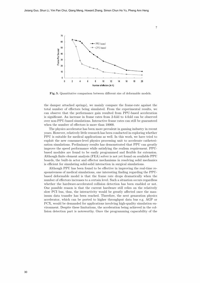
Fig. 4. Deformable model (a) layered construction of volumetric grid, (b) deformablegrid structure of bifurcation structure, and (c) a single-layered wire is inserted into thebi-layer structured catheter.
be understood as a variation of mass-spring-damper implementation. This pro-vides a convienient way for modeling linear solid mechancs. Most soft tissue,including the vessel wall, exhibit a non-linear stress-strain biomechanicial be-haviour [10][4][9]. To caputre this behaviour interactively, we extend the PPUbuilt-in model to an incremental-voigt model. In our model, two springs, eachwith an attached damper, are connected in parallel so that a biphasic biome-chanicial behaviour can be simulated.
As we are modeling the vessel tissue as a mass-spring system, data for thebiomechanical properties of vessel tissue serves, therefore, as a reference for thebehavior of the entire macroscopic mass-spring system, rather than the micro-scopic elasticity of individual single springs. To determine the micro-properties,we deploy our previously proposed optimization process [12] to compute themacroscopic elasticity of the whole mass-spring system which conforms withreal tissue biomechanics.
4 Simulation and Discussion
The guiding of the catheter/wire is a relatively complex component of the real-time simulation process since it involve interior interactions between the vesselwall and catheter and on the exterior as well. The solid-solid interaction ofthe vascular structure and catheter/ guidewire is resolved by the built-in PPUcollision detection mechanism. Various collision models have been adopted tospeed up the overall simulation performace. In order to increase the systemresponsiveness, a dual-model approach has been adopted for handling collisiondetection of the outer and inner layers. We apply a mesh-based collision modelfor the inner layer structures while the collision model for the outer layer is basedon a chain of spheres.
The PPU-based implementation has been compared with pure CPU-basedimplementation. Experiments are conducted on a Pentium 4 Dual Core 3.2HZPC equipped with NVIDIA GeForce 8800. The physics accelerator used is AGEIAPhysXP1. Fig. 5 shows a comparison of the frame rate between the two imple-mentations. Since the major physics computation is done on the effectors (i.e.
PPU-based deformable models for Catheterisation training
29
7
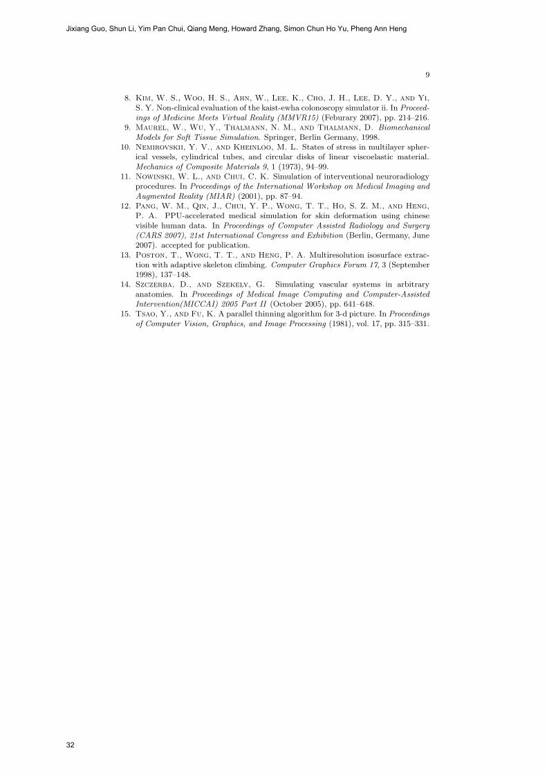
Fig. 5. Quantitative comparison between different size of deformable models.
the damper attached springs), we mainly compare the frame-rate against thetotal number of effectors being simulated. From the experimental results, wecan observe that the performance gain resulted from PPU-based accelerationis significant. An increase in frame rates from 2-fold to 4-fold can be observedover non-PPU-based simulations. Interactive frame rates can still be guaranteedwhen the number of effectors is more than 10000.
The physics accelerator has been more prevalent in gaming industry in recentyears. However, relatively little research has been conducted in exploring whetherPPU is suitable for medical applications as well. In this work, we have tried toexploit the new consumer-level physics processing unit to accelerate catheteri-sation simulations. Preliminary results has demonstrated that PPU can greatlyimprove the speed performance while satisfying the realism requirement. PPU-based modules are found to be easily programmed and flexible for extension.Although finite element analysis (FEA) solver is not yet found on available PPUboards, the built-in actor and effector mechanisms in resolving solid mechanicsis efficient for simulating solid-solid interaction in surgical simulations.
Although PPU has been found to be effective in improving the real-time re-sponsiveness of medical simulations, one interesting finding regarding the PPU-based deformable model is that the frame rate drops dramatically when thenumber of effectors increases to a certain level. Such a situation occurs regardlesswhether the hardware-accelerated collision detection has been enabled or not.One possible reason is that the current hardware still relies on the relativelyslow PCI bus, thus, the interactivity would be greatly affected once the max-imum data transfer has been reached. Therefore, the next genaration physicsaccelerator, which can be ported to higher throughput data bus e.g. AGP orPCX, would be demanded for applications involving high-quality simulation en-vironment. Despite these limitations, the acceleration being achieved in the col-lision detection part is noteworthy. Once the programming capacability of the
Jixiang Guo, Shun Li, Yim Pan Chui, Qiang Meng, Howard Zhang, Simon Chun Ho Yu, Pheng Ann Heng
30

8
hardware-accelerated physics computation (may be in the form of an interfaceto various numerical solvers) has become more flexible, the use of PPU in themedical community shall be more widely accepted.
In conclusion, a new deformable modeling framework has been proposed forthe medical simulation of catheterisation procedures. The framework is inte-grated with PPU so that interactive responsiveness can be achieved. Experi-mental results have demonstated the robustness of our proposed geometric de-formable vessel modeling framework. The next step of our work would be themodeling of other vascular interventional devices such as stent, balloon for simu-lation of angioplasty and stent implantation. In future work, we shall investigatethe possiblity of exploiting PPU to accelerate solid-fluid interaction. This wouldbe important for simulating blood-tissue interaction as well as blood-device in-teraction within different catheterisation procedures.
Acknowledgement
This work was supported by a grant from the Innovation and Technology Com-mission of the Hong Kong Special Administrative Region (Project No. UIM/174).This work is also affiliated with the Virtual Reality, Visualization and Imag-ing Research Center at The Chinese University of Hong Kong as well as theMicrosoft-CUHK Joint Laboratory for Human-Centric Computing and InterfaceTechnologies.
References
1. Bloomenthal, J. Calculation of reference frames along a space curve. GraphicsGem (1990), 567–571.
2. Cotin, S., Duriez, C., Lenoir, J., Neumann, P., and Dawson, S. New ap-proaches to catheter navigation for interventional radiology simulation. In Proceed-ings of Medical Image Computing and Computer-Assisted Intervention(MICCAI)2005 Part II (October 2005), pp. 534–542.
3. Fiedler, M. J., Chen, S. J., Judkins, T. N., Oleynikov, D., and Stergiou,
N. Virtual reality for robotic laparoscopic surgical training. In Proceedings ofMedicine Meets Virtual Reality (MMVR15) (Feburary 2007), pp. 127–129.
4. Fung, Y. C. Biomechanics: Mechanical Properties of Living Tissues, second ed.Springer, Berlin Germany, 1993.
5. Harders, M., Steinemann, D., Gross, M., and Szekely, G. A hybrid cutingapproach for hysterscopy simulation. In Proceedings of Medical Image Computingand Computer-Assisted Intervention(MICCAI) 2005 (October 2005), pp. 567–574.
6. Heng, P. A., Cheng, C. Y., Wong, T. T., Xu, Y. S., Chui, Y. P., Chan,
K. M., and Tso, S. K. A virtual reality training system for knee arthroscopicsurgery. IEEE Transactions on Information Technology in Biomedicine 8, 2 (June2004), 217–227.
7. Ikeda, S., Arai, F., Fukuda, T. Negoro, M., Irie, K., and Takahashi, I. Anin vitro patient-tailored model of human cerebral artery for simulating endovascularintervention. In Proceedings of Medical Image Computing and Computer-AssistedIntervention(MICCAI) 2005 Part I (October 2005), pp. 925–932.
PPU-based deformable models for Catheterisation training
31
9
8. Kim, W. S., Woo, H. S., Ahn, W., Lee, K., Cho, J. H., Lee, D. Y., and Yi,
S. Y. Non-clinical evaluation of the kaist-ewha colonoscopy simulator ii. In Proceed-ings of Medicine Meets Virtual Reality (MMVR15) (Feburary 2007), pp. 214–216.
9. Maurel, W., Wu, Y., Thalmann, N. M., and Thalmann, D. BiomechanicalModels for Soft Tissue Simulation. Springer, Berlin Germany, 1998.
10. Nemirovskii, Y. V., and Kheinloo, M. L. States of stress in multilayer spher-ical vessels, cylindrical tubes, and circular disks of linear viscoelastic material.Mechanics of Composite Materials 9, 1 (1973), 94–99.
11. Nowinski, W. L., and Chui, C. K. Simulation of interventional neuroradiologyprocedures. In Proceedings of the International Workshop on Medical Imaging andAugmented Reality (MIAR) (2001), pp. 87–94.
12. Pang, W. M., Qin, J., Chui, Y. P., Wong, T. T., Ho, S. Z. M., and Heng,
P. A. PPU-accelerated medical simulation for skin deformation using chinesevisible human data. In Proceedings of Computer Assisted Radiology and Surgery(CARS 2007), 21st International Congress and Exhibition (Berlin, Germany, June2007). accepted for publication.
13. Poston, T., Wong, T. T., and Heng, P. A. Multiresolution isosurface extrac-tion with adaptive skeleton climbing. Computer Graphics Forum 17, 3 (September1998), 137–148.
14. Szczerba, D., and Szekely, G. Simulating vascular systems in arbitraryanatomies. In Proceedings of Medical Image Computing and Computer-AssistedIntervention(MICCAI) 2005 Part II (October 2005), pp. 641–648.
15. Tsao, Y., and Fu, K. A parallel thinning algorithm for 3-d picture. In Proceedingsof Computer Vision, Graphics, and Image Processing (1981), vol. 17, pp. 315–331.
Jixiang Guo, Shun Li, Yim Pan Chui, Qiang Meng, Howard Zhang, Simon Chun Ho Yu, Pheng Ann Heng
32
3D FEM/XFEM-based Biomechanical BrainModeling for Preoperative Image Update
Lara M. Vigneron1, Romain C. Boman2, Jean-Philippe Ponthot2,Pierre A. Robe3, Simon K. Warfield4, and Jacques G. Verly1
1 Department of Electrical Engineering and Computer Science,2 Department of Mechanical Engineering,
3 Department of Neurosurgery, University Hospital,University of Liege, Liege, Belgium;
4 Computational Radiology Laboratory, Children’s Hospital,Harvard Medical School, Boston, MA, USA.
Abstract. We present an end-to-end system for updating 3D preope-rative images in the presence of brain shift and successive resections. Thetissue discontinuities due to resections are handled via the eXtented Fi-nite Element Method (XFEM), which has the appealing feature of han-dle arbitrarily-shaped discontinuity without any remeshing. The mainnovelty of the paper lies in the use of XFEM in 3D.
1 Introduction
The main goal of brain surgery is to remove as much as possible of lesional tis-sues, while avoiding contacts with eloquent areas and white matter fiber tracts.Surgery is planned on the basis of preoperative images of multiple modalities,such as CT, sMRI, fMRI, PET, DTI, and is generally performed using an image-guided navigation system that relates the 3D preoperative images to patient co-ordinates. However, throughout surgery, the brain deforms, mostly as a resultof the leakage of the cerebrospinal fluid out of the skull cavity and of surgicalacts, such as retraction and resection. As surgery progresses, preoperative imagesbecome progressively less representative of the brain, and navigation accuracydecreases. One solution is to evaluate brain deformations from reduced-qualityintraoperative images acquired at several critical points during surgery, and toupdate, i.e. to deform, all high-quality preoperative images using a nonrigid reg-istration.
One category of nonrigid registration techniques uses physics-based models.Prior to surgery, a biomechanical brain model specific to the patient is builtfrom preoperative images. The model consists of a 3D volume mesh and oneor more mechanical-behavior laws. A number of key anatomical landmarks areextracted and tracked through successive intraoperative images. The biomechan-ical model is deformed, generally based on the Finite Element Method (FEM),in accordance with the displacement fields of these landmarks. The resultingdeformation is then used to update the preoperative images.
Most studies of brain deformation based on biomechanical models have focusedon the early stages of surgery, i.e. prior to any significant deformation and anycut [1–4]. The reported accuracy for deformation prediction is about 1 voxel. Thesituation becomes more complex when the surgeon performs cuts, retractions,
33
or resections [1, 5, 6], the last two necessarily involving a cut. The main diffi-culty associated with a cut is the discontinuity it implies in the tissue. Indeed,FEM cannot handle such discontinuities directly and, consequently, FEM hasto be used in conjunction with mesh adaptation [7] or remeshing [8] techniques.However, it is likely that current remeshers, mainly developed for mechanicalengineering applications, would not work properly on irregular objects such asa brain (which is furthermore extracted from an image), especially in a auto-matic mode. While human intervention may improve results, the time requiredis significant and unpredictable, which makes it unsuitable for surgery where atimely response is essential.
Besides FEM, other methods have also been employed in the medical field tomodel tissue discontinuities, like the boundary element method (BEM) [9] andmeshless methods [10, 11]. We propose an approach based on the eXtended Fi-nite Element Method (XFEM or X-FEM) [12]. This method allows the objectto be modeled by finite elements without explicitly meshing the discontinuities,which can then be located arbitrary with respect to the underlying finite-elementmesh. Here, we describe, and report on the performance of, a 3D FEM- andXFEM-based end-to-end system capable of updating preoperative images in thepresence of brain shift followed by successive resections [13]. The main noveltyis that the problem is treated in 3D.
The structure of the paper is as follows. In Sect. 2, we introduce the basicprinciples of FEM and XFEM. In Sect. 3, we describe our preoperative image-update system and underlying algorithms. In Sect. 4, we show our results for onepatient case, while, in Sect. 5, we validate our results. In Sect. 6, we concludeand point out future work.
2 Basic principles of FEM and XFEM
We have to solve the static problem of finding the displacement field that corre-sponds to the deformation of a solid (a brain in the present case), subjected toexternal forces. With FEM, the solid is discretized into a mesh, i.e. into a set afinite elements interconnected by nodes, and the displacement field is approxi-mated by
uFEM (x) =∑iεI
ϕi(x)ui, (1)
where I is the set of nodes, the ϕi’s are the nodal shape functions (NSFs), andthe ui’s are nodal degrees of freedom (DOFs).
In Eq. (1), each NSF ϕi(x) is defined as being continuous over each FE, im-plying the same property for the displacement field uFEM (x). Furthermore, thedisplacement ui at any node can only take a single value. Consequently, thehandling of a discontinuity with FEM requires one to align the discontinuitywith element boundaries and to duplicate the nodes lying on these boundaries.These operations can be performed by mesh adaptation or remeshing.
XFEM [12, 14] handles a discontinuity by allowing the displacement field to
Lara M. Vigneron, Romain C. Boman, Jean-Philippe Ponthot, Pierre A. Robe, Simon K. Warfield, and Jacques G. Verly
34

be discontinuous within mesh elements. Arbitrarily-shaped discontinuities canthen be modeled without any remeshing. The XFEM displacement field is ap-proximated by generalizing the FEM displacement field (1) with
uXFEM (x) =∑iεI
ϕi(x)ui +∑iεJ
ϕi(x)nEi∑j=1
gj(x)aji. (2)
The first term corresponds to the FEM displacement field approximation (1),where I is the set of nodes, the ϕi(x)’s the FEM NSFs, and the ui’s the nodalFEM DOFs. The key of XFEM is the “enrichment” that adds a number, nEi ,of DOFs aji to each node i of set J , which is the subset of nodes of I whosesupport is intersected by the discontinuity. These DOFs are multiplied by theNSFs ϕi(x) and the discontinuous functions gj(x). The simplest choice for thegj(x)’s is a piecewise-constant function that changes sign at the discontinuity,i.e. the Heaviside function
H(x) ={
1 for (x− x∗).en > 0−1 for (x− x∗).en < 0, (3)
where x is a point of the solid, x∗ is the point on the discontinuity that is theclosest to x, and en is the outward normal to the discontinuity at x∗.
Figure 1 illustrates the use of 2D XFEM for a mesh cut horizontally, with eachpart being subjected to a distinct translation. This example shows that the twoparts of the mesh can move independently without one having to remesh theobject along the discontinuity.
(a) (b)
Fig. 1. Example of 2D XFEM calculation. (a) FE mesh and discontinuity geometriesprior to deformation. (b) Deformation results provided by XFEM when top and bottomparts are subjected to distinct translations.
3 MethodsThe inputs are (1) a set of multimodality preoperative images and (2) a sequenceof intraoperative MR (iMR) T1 images, acquired with a 0.5 Tesla intraopera-tive GE Signa scanner5. The protocol of iMR acquisition is defined such thatthe 1st iMR image is acquired prior to the opening of the skull. Before surgery,a patient-specific biomechanical model is built from the set of preoperative im-ages. Once the 1st iMR image is acquired, the set of preoperative images and thebiomechanical model are brought into the intraoperative coordinate system bya rigid registration. Without any loss of generality, we deal with the problem ofupdating the 1st iMR image, which thus plays the role of a fictive preoperative5 iMR image size is 256× 256× 60 voxels; voxel size is 0.9375× 0.9375× 2.5 mm.
3D FEM/XFEM-based Biomechanical Brain Modeling for Preoperative Image Update
35

image. Except for the rigid registration between the preoperative images, thebiomechanical model, and the 1st iMR image, all key aspects of the system canbe discussed and illustrated.
To build the biomechanical model, we proceed as follows. From the 1st iMRimage (once again, as a substitute for true preoperative images), we manuallysegment out the cortex and the tumor using 3D Slicer
6, and smooth both re-gions. Then, we mesh the cortex surface with triangles using Isosurf
7. Besides,we define a set of points lying on the tumor boundary. Based on the cortextriangular mesh surface and this set of points, we mesh the cortex volume withtetrahedra using Tetgen
8. We do not create a surface mesh of the tumor bound-ary because Tetgen cannot handle internal surfaces. Finally, we assign to thismesh a homogeneous linear elastic (E = 7kPa, ν = 0.45)9 behavior law.
To drive the deformation of the biomechanical model, we track the surface de-formation of the cortex and tumor through successive pairs of iMR images. Forthis purpose, we segment out the cortex and tumor from each iMR image using3D Slicer and smooth both regions. The matching of corresponding surfaces isperformed with an active surface algorithm [1]. The resulting surface displace-ments fields are applied to the biomechanical model, and its deformations arecomputed using FEM or XFEM, depending upon the type of circumstances, e.g.brain shift or resection. We developed our FEM and XFEM codes within thesoftware Metafor
10. For each (X)FEM computation, we assume a zero initialstress. We perform FEM computations in a nonlinear formulation (large defor-mations) because this has been shown to provide better results than in a linearformulation (small deformations) [15], and to reduce the problem of elementflipping. By contrast, we perform XFEM computations in a linear formulation,because a XFEM nonlinear formulation is not yet available. The set of preoper-ative images (the 1st iMR image in our case) are deformed, i.e. warped, basedon the volume displacement field of the biomechanical model. We use VTK
11
and ITK12 for all image processing.
4 Results
The top row of Fig. 3 shows a sequence of five iMR images. The 1st image wasacquired prior to the opening of the skull. The 2nd image was acquired afterthe opening of the skull and dura, and shows some brain shift. The 3rd and4th images were acquired after each of two successive resections. The 5th imagewas acquired at the end of the surgery after the 3rd resection, and shows some
6 www.slicer.org/7 http://mi.eng.cam.ac.uk/ gmt11/software/isosurf/isosurf.html8 http://tetgen.berlios.de/9 Experiments show that our current implementation appear sensitive to the values of
the parameters, in particular that of E: some values of E have indeed been observedto cause element flipping.
10 http://garfield.ltas.ulg.ac.be/oo meta/11 www.vtk.org12 www.itk.org
Lara M. Vigneron, Romain C. Boman, Jean-Philippe Ponthot, Pierre A. Robe, Simon K. Warfield, and Jacques G. Verly
36

(a) (b)
Fig. 2. (a) Initial active surface with color levels corresponding to the magnitude ofthe final displacements. The location of the brain shift is clearly visible. (Discussed inSect. 4.1.) (b) Deformed mesh resulting from the XFEM-based modeling of the 2nd
resection. (Discussed in Sect. 4.3.)
postoperative brain shift. The modeling of brain shift, 1st, 2nd, and 3rd resectionare performed using different techniques, as detailed below.
4.1 Modeling of brain shift via FEM
To model brain shift, we estimate the surface displacement field of the cortexand tumor, and use them to deform the biomechanical model. For the cortex, theinitial active surface corresponds to the surface of the biomechanical model. Oncethe result of the active surface algorithm is obtained (Fig. 2a), the displacementsof the active surface nodes are directly applied to the cortex nodes. For thetumor, the displacements are applied differently because the tumor is not definedby a surface mesh. An active surface computation is performed on the healthybrain (defined as the whole brain minus the tumor). Then, we apply, to thenodes of the volume mesh located along the tumor boundary, displacementsextrapolated from the surface displacement field of the active surface along thetumor boundary. In the present case, no tissue discontinuity is involved, so thevolume deformation is computed via FEM. The resulting volume displacementfield is used to warp the whole brain image extracted from the 1st iMR image.The result is shown in Fig. 3.2b.
4.2 Modeling of 1st resection via FEM
Matching two surfaces to get a displacement field makes sense only if the sur-faces correspond to the same physical entity. In the case of resection, we cannotrely on the totality of the cortex surface, since a part of it is now missing. Con-sequently, we evaluate the displacement field for the combined surfaces of theintact cortex and of the tumor, which effectively constitutes the boundary sur-face of the healthy brain.
Based on the 2nd and 3rd iMR images, we cannot determine the volume andlocation of the tissue removed by the resection. This is because the 3rd iMR im-age shows the combined effect of tissue removal and subsequent deformation. Infact, because the 2nd and 3rd iMR images do not show the same volume of braintissue, the problem of modeling resection and brain shift is fundamentally dif-ferent. Nevertheless, we decided to model the 1st resection by still relying on thedisplacement fields of key surfaces, here the healthy-brain boundary, to deform
3D FEM/XFEM-based Biomechanical Brain Modeling for Preoperative Image Update
37

the biomechanical model. This indeed appears to be the only reliable informa-tion concerning the deformation due to resection that we can extract from the2nd and 3rd iMR images. Consequently, we do not model explicitly the removalof tissue, but we model directly the deformation resulting from it, without intro-ducing any tissue discontinuity. Using the displacement field of the healthy brainboundary, we compute the deformation of the biomechanical model via FEM.Then, using the resulting volume displacement field, we warp the fictive preoper-ative image in its current state of update (Fig. 3.2b), in the same way as for brainshift. The resulting image is shown in Fig. 3.3b, which is now registered to the3rd iMR image (Fig. 3.3a), except outside of the healthy-brain boundary, i.e. forthe tumor. Finally, we alter the resulting image to reflect the effect of resection.For this, we assign the background color to the voxels of Fig. 3.3b correspondingto the resected tissue volume “absent” in the 3rd iMR image (Fig. 3.3a). Theresult of the warping with resection, performed by masking the warped image(Fig. 3.3b) with the segmentation of the whole brain from the 3rd iMR image(Fig. 3.3a), is shown in Fig. 3.3c.
4.3 Modeling of 2nd resection via XFEM
The significant feature of the 2nd resection is that some tissue has already beenremoved by the 1st resection, which means that this tissue cannot have anyphysical influence on subsequent brain deformations because it does not “exist”anymore. Consequently, the 1st resection must be reflected in the biomechanicalmodel. Recall that, to model the 1st resection, the biomechanical model has beendeformed to be registered to the 3rd iMR image. So, using the 3rd iMR image,we can define the boundary of the 1st resection, i.e. the tissue discontinuity toinclude in the biomechanical model. With a FEM-based biomechanical model,we would remesh the model to take into account the discontinuity. Then, wewould just remove the part of the mesh corresponding to the resected tissue,and use the other part of the mesh to model the 2nd resection. Instead, withXFEM, we enrich the nodes whose support is intersected by the discontinuitywith XFEM Heaviside DOFs. Consequently, when the XFEM-based biomechan-ical model deforms, the part corresponding to tissue removed by the 1st resectionhas no influence on the deformation of the remaining part of the brain.
Except for the fact the biomechanical model is deformed with XFEM ratherthan FEM, the modeling of 2nd resection is identical to that of the 1st resec-tion. The biomechanical model is deformed in accordance with the displacementfield of the healthy-brain boundary evaluated from the 3rd and 4th iMR images.Fig. 2b shows the deformed mesh, result of the XFEM computation. The bot-tom part of the mesh, representing the tissue remaining after the 1st resection,was deformed according to the displacement field of the healthy brain boundary,while the top part, representing the tissue removed by the 1st resection, wassubjected to a translation, but only for visualization purposes. The two parts ofthe mesh could indeed overlap around the discontinuity after deformation of thebottom part. Using the XFEM volume displacement field, we warp the fictivepreoperative image in is current state of update (Fig. 3.3b). The resulting imageis shown in Fig. 3.4b, while the result of the warping with resection, performed
Lara M. Vigneron, Romain C. Boman, Jean-Philippe Ponthot, Pierre A. Robe, Simon K. Warfield, and Jacques G. Verly
38
by masking Fig. 3.4b with the segmentation of the whole brain from the 4th iMRimage (Fig. 3.4a), is shown in Fig. 3.4c.
4.4 Modeling of 3rd resection via XFEM
If we had complete freedom, we would model the 3rd resection and postoperativebrain shift based on the bottom part of the output mesh of the 2nd resectionmodeling (Fig. 2b). However, even though the mesh is displayed as two separateparts, it is, in fact, a single entity. Indeed, a main feature of XFEM is to beable to handle the effect of a discontinuity without modifying the underlyingmesh, i.e. without remeshing. For modeling the 2nd resection, the edges of ele-ments straddling the discontinuity have been “cut” and their nodes moved apart.However, it is not possible to start an XFEM calculation with a mesh alreadydeformed because the finite elements are not supposed to be already cut. Conse-quently, XFEM, expressed in linear formulation, does not permit us to proceedwith a new discontinuity from a configuration already deformed by XFEM. In-deed, we should use a nonlinear formulation of XFEM [16] to proceed as desired.
For temporarily avoiding going nonlinear, we devised a new method that con-tinues to preserve the spirit of XFEM, which is mainly to avoid remeshing inthe presence of a discontinuity. However, this method implies additional process-ing. The idea of our method is “to reconnect the pieces” of the deformed mesh(Fig. 2b), but without remeshing, in such a way we can further resect it. Since wealready have the correct deformed coordinates for the bottom part of the mesh,we need to find a way “to restore” a meaningful top part. We cannot simplylower the top part of the mesh, because it would not fit the bottom part. Indeed,the bottom part has been deformed during the modeling of the 2nd resection,with consequence that the discontinuity surface of the bottom part has changedshape. While this might not be the best from a computational standpoint, ourcurrent solution is to use, for the coordinates of the nodes of the top part ofthe mesh, the coordinates that we would had got if we had modeled the 2nd
resection based on FEM, rather than on XFEM, i.e. without taking into accountthe removal of tissue by the 1st resection. These coordinates are erroneous, butthis is not an issue, since these nodes will again be resected, given that the 3rd
resection is necessarily deeper than the 2nd resection. We must be careful to en-sure that the restored elements have good aspect-ratios. FEM is a way to achievethis, although there is no guarantee that good results will be obtained for thecomposite elements straddling the discontinuity.
After the reconnection of the mesh, the modeling of the 3rd resection is identicalto that of the 2nd resection. The tissue discontinuity due to the 2nd resection isdefined from the 4th iMR image, and used to enrich the nodes of the reconnectedmesh. The biomechanical model is deformed based on XFEM in accordance withthe displacement field of the healthy-brain boundary computed from the 4th and5th iMR images. One significant feature of the procedure described for modelingthe 3rd resection, i.e. mesh reconnection followed by model deformation, is thatit can be applied iteratively for each subsequent resection visible on successiveiMR images, no matter how many there are.
3D FEM/XFEM-based Biomechanical Brain Modeling for Preoperative Image Update
39
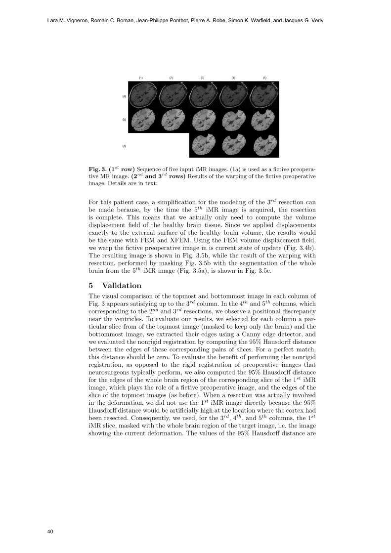
Fig. 3. (1st row) Sequence of five input iMR images. (1a) is used as a fictive preopera-tive MR image. (2nd and 3rd rows) Results of the warping of the fictive preoperativeimage. Details are in text.
For this patient case, a simplification for the modeling of the 3rd resection canbe made because, by the time the 5th iMR image is acquired, the resectionis complete. This means that we actually only need to compute the volumedisplacement field of the healthy brain tissue. Since we applied displacementsexactly to the external surface of the healthy brain volume, the results wouldbe the same with FEM and XFEM. Using the FEM volume displacement field,we warp the fictive preoperative image in is current state of update (Fig. 3.4b).The resulting image is shown in Fig. 3.5b, while the result of the warping withresection, performed by masking Fig. 3.5b with the segmentation of the wholebrain from the 5th iMR image (Fig. 3.5a), is shown in Fig. 3.5c.
5 Validation
The visual comparison of the topmost and bottommost image in each column ofFig. 3 appears satisfying up to the 3rd column. In the 4th and 5th columns, whichcorresponding to the 2nd and 3rd resections, we observe a positional discrepancynear the ventricles. To evaluate our results, we selected for each column a par-ticular slice from of the topmost image (masked to keep only the brain) and thebottommost image, we extracted their edges using a Canny edge detector, andwe evaluated the nonrigid registration by computing the 95% Hausdorff distancebetween the edges of these corresponding pairs of slices. For a perfect match,this distance should be zero. To evaluate the benefit of performing the nonrigidregistration, as opposed to the rigid registration of preoperative images thatneurosurgeons typically perform, we also computed the 95% Hausdorff distancefor the edges of the whole brain region of the corresponding slice of the 1st iMRimage, which plays the role of a fictive preoperative image, and the edges of theslice of the topmost images (as before). When a resection was actually involvedin the deformation, we did not use the 1st iMR image directly because the 95%Hausdorff distance would be artificially high at the location where the cortex hadbeen resected. Consequently, we used, for the 3rd, 4th, and 5th columns, the 1st
iMR slice, masked with the whole brain region of the target image, i.e. the imageshowing the current deformation. The values of the 95% Hausdorff distance are
Lara M. Vigneron, Romain C. Boman, Jean-Philippe Ponthot, Pierre A. Robe, Simon K. Warfield, and Jacques G. Verly
40
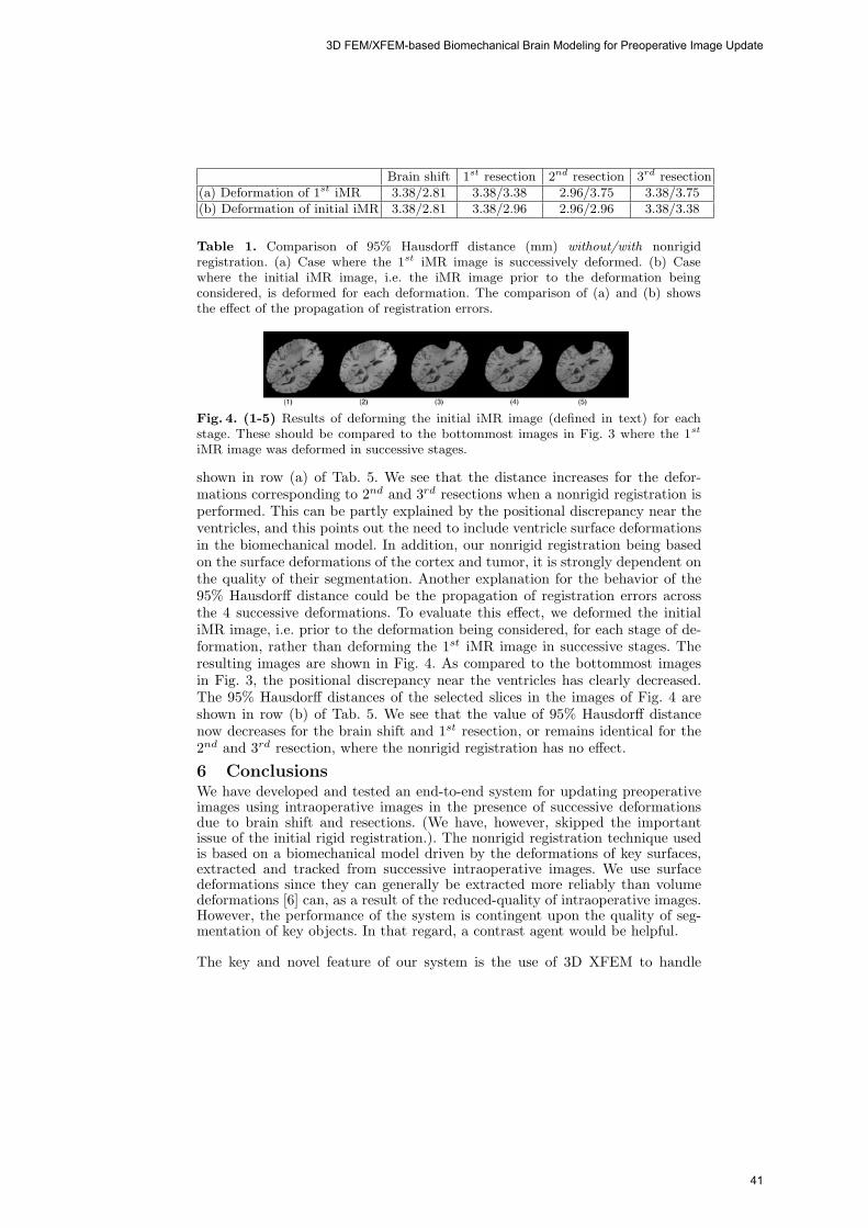
Brain shift 1st resection 2nd resection 3rd resection(a) Deformation of 1st iMR 3.38/2.81 3.38/3.38 2.96/3.75 3.38/3.75(b) Deformation of initial iMR 3.38/2.81 3.38/2.96 2.96/2.96 3.38/3.38
Table 1. Comparison of 95% Hausdorff distance (mm) without/with nonrigidregistration. (a) Case where the 1st iMR image is successively deformed. (b) Casewhere the initial iMR image, i.e. the iMR image prior to the deformation beingconsidered, is deformed for each deformation. The comparison of (a) and (b) showsthe effect of the propagation of registration errors.
Fig. 4. (1-5) Results of deforming the initial iMR image (defined in text) for eachstage. These should be compared to the bottommost images in Fig. 3 where the 1st
iMR image was deformed in successive stages.
shown in row (a) of Tab. 5. We see that the distance increases for the defor-mations corresponding to 2nd and 3rd resections when a nonrigid registration isperformed. This can be partly explained by the positional discrepancy near theventricles, and this points out the need to include ventricle surface deformationsin the biomechanical model. In addition, our nonrigid registration being basedon the surface deformations of the cortex and tumor, it is strongly dependent onthe quality of their segmentation. Another explanation for the behavior of the95% Hausdorff distance could be the propagation of registration errors acrossthe 4 successive deformations. To evaluate this effect, we deformed the initialiMR image, i.e. prior to the deformation being considered, for each stage of de-formation, rather than deforming the 1st iMR image in successive stages. Theresulting images are shown in Fig. 4. As compared to the bottommost imagesin Fig. 3, the positional discrepancy near the ventricles has clearly decreased.The 95% Hausdorff distances of the selected slices in the images of Fig. 4 areshown in row (b) of Tab. 5. We see that the value of 95% Hausdorff distancenow decreases for the brain shift and 1st resection, or remains identical for the2nd and 3rd resection, where the nonrigid registration has no effect.
6 ConclusionsWe have developed and tested an end-to-end system for updating preoperativeimages using intraoperative images in the presence of successive deformationsdue to brain shift and resections. (We have, however, skipped the importantissue of the initial rigid registration.). The nonrigid registration technique usedis based on a biomechanical model driven by the deformations of key surfaces,extracted and tracked from successive intraoperative images. We use surfacedeformations since they can generally be extracted more reliably than volumedeformations [6] can, as a result of the reduced-quality of intraoperative images.However, the performance of the system is contingent upon the quality of seg-mentation of key objects. In that regard, a contrast agent would be helpful.
The key and novel feature of our system is the use of 3D XFEM to handle
3D FEM/XFEM-based Biomechanical Brain Modeling for Preoperative Image Update
41
tissue discontinuities without having to resort to remeshing. For a biomechani-cal model as simple as the one used here for illustration purposes, it would bestraightforward to build a new model for each deformation. However, our goal isto include as much information as possible from preoperative images and, as aresult, to use our system with complex biomechanical models. The modeling ofdiscontinuities will then surely involve some remeshing, and in that case, XFEMcould be a good alternative. While dealing with a one-time resection is relativelystraightforward with XFEM, we have found that XFEM expressed in a linearformulation cannot deal with successive resections. However, this paper showsan effective method for going around this problem. The results obtained give usconfidence that the approach proposed works correctly. A nonlinear formulationof XFEM should provide a more systematic approach for dealing with succes-sive resections. In future work, we will examine the XFEM nonlinear formulation.
Acknowledgements This investigation was supported in part by the “Fonds Na-tional de la Recherche Scientifique (F.N.R.S.)”, Brussels, Belgium, by NSF grant ITR0426558, a research grant from CIMIT, by NIH grants R03 CA126466 and R01 RR021885.
References
1. Ferrant, M., et al.: Serial registration of intra-operative MR images of the brain.Med. Image Anal. 6 (2002) 337–359
2. Miller, K., et al.: Towards computing brain deformations for diagnosis, prognosisand neurosurgical simulation. J. Mech. Med. Biol. 5(1) (2005) 105–121
3. Paulsen, K., et al.: A computational model for tracking subsurface tissue defor-mation during stereotactic neurosurgery. IEEE Trans. Biom. Eng. 46(2) (1999)213–225
4. Warfield, S.K., et al.: Capturing intraoperative deformations: research experienceat Brigham and Women’s Hospital. Med. Image Anal. 9(2) (2005) 145–162
5. Miga, M.I., et al.: Modeling of retraction and resection for intraoperative updatingof images. Neurosurgery 49(1) (2001) 75–84
6. Clatz, O., et al.: Robust non-rigid registration to capture brain shift from intra-operative MRI. IEEE Trans. Medical Imaging 24(11) (2005) 1417–1427
7. Serby, D., et al.: A new approach to cutting into finite element models. MICCAI’012208 (2001) 425–433
8. Nienhuys, H.W.: Cutting in deformable objects. PhD thesis, Institute for Infor-mation and Computing Sciences, Utrecht University (2003)
9. Ecabert, O., et al.: Brain shift correction based on a boundary element biome-chanical model with different material properties. MICCAI’03 2878 (2003) 41–49
10. De, S., et al.: On the method of finite spheres in applications: Towards the use withADINA and in a surgical simulator. Computational Mechanics 31 (2003) 27–37
11. Liu, H., Shi, P.: Meshfree representation and computation: Applications to cardiacmotion analysis. IPMI 18 (2003) 560–72
12. Moes, et al.: A finite element method for crack growth without remeshing. Int. J.Numer. Meth. Engng. 46 (1999) 131–150
13. Vigneron, L.M., et al.: XFEM-based modeling of successive resections for preop-erative image updating. SPIE Medical Imaging 5367 (2006) 735–746
14. Sukumar, N., Prevost, J.H.: Modeling quasi-static crack growth with the extendedfinite element method. Part I: Computer implementation. Int. J. Solids and Struc-tures 40(26) (2003) 7513–7537
15. Hawkins, T., et al.: Comparison of constitutive models of brain tissue for non-rigidimage registration. 2nd Workshop on Computer Assisted Diagnosis and Surgery(2006)
16. Legrain, G., et al.: Stress analysis around crack tips in finite strain problems usingthe extended finite element method. Int. J. Numer. Meth. Engng. 63(2) (2005)290–314
Lara M. Vigneron, Romain C. Boman, Jean-Philippe Ponthot, Pierre A. Robe, Simon K. Warfield, and Jacques G. Verly
42

Spherical Harmonics 3D Active Contours for Membrane Bilayer- Bound Surfaces
Khaled Khairy*, Jacques Pecreaux*, Jonathon Howard
Max-Planck Institute of Molecular Cell Biology and Genetics, Dresden, Germany
* These authors contributed equally to this work.
Abstract: Active contours is a powerful image segmentation technique based on simultaneously optimizing the overlap of a surface contour with the intensity image (external energy) on the one hand, and a constraining image-independent penalty based on the first and second derivatives of the contour (internal energy) on the other. Although the above form is applicable to a wide class of images, including prior information about the topology and smoothness as well as insights from physical theories regarding specific material properties of the object under study are expected to result in faster and more accurate segmentations.
In this work we extend the formulation of the active contour internal energy for the common case of 3D-imaging lipid-bilayer membrane-bound objects of topological genus zero. Examples include organelles, cells and artificial vesicles. In the non-supervised method presented here, the internal energy takes into account membrane bending elasticity as well as constraints imposed by the fact that the two bilayer leaflets are allowed to slide relative to each other. An additional topology constraint is implicitly accounted for by using a spherical harmonics parametric contour representation. The balance between internal and external energies (i.e. the regularization parameter) is determined using the L-curve method.
To ensure convergence and numerical stability a good starting guess for the contour is essential. We show in detail a method, that also makes use of the L-curve, for calculating this guess, and apply the complete procedure to a representative synthetic data set using realistic physical quantities based on membrane biophysical theories and known experimental results.
1 Introduction
Active contours [1] have been used extensively as a means for automatic and accurate image segmentation. The main idea is to allow a contour that is superimposed on the image to change shape until it minimizes a cost functional (E) that takes the form
43
internal externalE E E�� � (1)
with internalE a shape prior that enforces smoothness constraints and typically depends
on the first and higher derivatives of the contour, externalE a quantity sensitive to the amount of overlap of the contour with the intensity values of the image, and � a parameter that balances the relative importance of the two terms. Equation 1 is generally applicable in 2 and 3 space dimensions. Implementations of the method differ in the choice for �, the exact forms for internalE and externalE , and the mathematical description of the contour. Subjective choices of � and physically unrealistic forms for internalE result in convergence to suboptimal shapes. This problem has partially been alleviated by the introduction of statistical shape models (see for example [2]), which constrain the contour search to a subset of the shapes allowed by the shape description. However, statistical shape models require a training set and may impose constraints that are too stringent for detecting significant variations in shape. Most importantly, they generally do not provide a natural connection to the underlying biophysics that gave rise to a particular shape. Therefore we will address the issue of segmenting 3D intensity images in the context of Equation 1, when the object under study has —at least partially —known mechanical properties.
1.1 Incorporation of Prior Information into the Active Contour Procedure
In this paper, we focus on objects that are bounded by lipid membrane bilayers. Examples include organelles, cells and artificial bilayer vesicles (liposomes). For these objects biophysical theories [3] and experimental mechanical measurements [4-6] provide prior information that can be incorporated into our edge-finding procedure. The theoretical predictions alone are already able to reproduce shapes that closely resemble experimental observations both qualitatively [7] and quantitatively [8] in cases where the membrane bilayer is expected to primarily determine the morphology (Fig.1a).
internalE of Equation 1 is an appropriate vehicle for incorporating such prior information [9], which primarily depends on the membrane bending elasticity and the resistance of the area difference between the bilayer leaflets to deviate from some preferred value (Fig.1b). Fig.1a shows some of the “default” shapes that the active contour will tend to when such an internalE is minimized on its own.
Moreover, the topology of such biological objects is often restricted to that of the sphere. This piece of prior information we implicitly include by using a spherical harmonics parameterization (SHP) of the surface [10]. The spherical harmonics are the 3D equivalent of the Fourier series defined on the surface of a sphere (see below).
Khaled Khairy, Jacques Pecreaux, Jonathon Howard
44
1.2 Other Issues: Regularization and the Starting Shape
To avoid artificially favoring internalE over externalE or vice versa, we use an objective way for determining the regularization parameter���in Equation 1, namely the L-curve method [11], which determines � as the point of maximum curvature on the curve obtained when plotting the logarithm of internalE vs. the logarithm of externalE when performing the optimization for a series of values of the regularization parameter.
However, before optimizing Equation 1, we need a good starting set of shape coefficients to improve convergence and numerical stability. To obtain such a set we map an initial surface triangulation (obtained for instance by using a marching cubes algorithm) to the unit sphere [12, 13]. In this article we introduce a method of spherical mapping that also benefits from the objectivity of the L-curve procedure.
Our complete method is illustrated on a noisy synthetic 3D intensity data set that simulates 3D fluorescence microscopy images of a human red blood cell discocyte. To our knowledge, this is the first demonstration of 3D active contours based on membrane biophysics.
2 Theory
2.1 Membrane-biophysics-derived (internal) Energies
Here we give the expressions used to calculate the internal (image-independent) energy of the contour, when we know that the observed object is bounded by a lipid-bilayer membrane. Theoretically the shape of a membrane bilayer contour is assumed to minimize an energy functional (E) that –among other possible contributions–includes the bending energy of the membrane (Eb) [14], and the area difference elasticity energy (EADE), which is the resistance of the area difference between the outer and inner leaflets (�A) to deviations from some preferred value (�Ao)[15-18].
internal b ADEE E E� � (2)
The first term is given by,
2b
S
(2 )2b oE H C dA�
� � (3)
where b� (~25x10-20J [5]) is the bending modulus, H is the local curvature, and oCis the preferred curvature. oC is a local term that depends on the local lipid composition and lipid molecule geometry (Fig.1b). The second term in Equation 1 is given by
Spherical Harmonics 3D Active Contours for Membrane Bilayer- Bound Surfaces
45
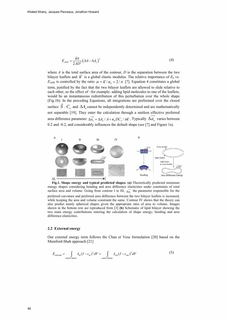
� �222ADE oE A A
AD�
� � � (4)
where A is the total surface area of the contour, D is the separation between the two bilayer leaflets and � is a global elastic modulus. The relative importance of Eb vs. EADE is controlled by the ratio / 2 /b� � � � � [7]. Equation 4 constitutes a global term, justified by the fact that the two bilayer leaflets are allowed to slide relative to each other, so the effect of –for example- adding lipid molecules to one of the leaflets, would be an instantaneous redistribution of this perturbation over the whole shape (Fig.1b). In the preceding Equations, all integrations are performed over the closed surface S
�. oC and oA� cannot be independently determined and are mathematically
not separable [19]. They enter the calculation through a unitless effective preferred area difference parameter / /o o b oa A A DC� �� � � � . Typically oa� varies between 0.2 and -0.2, and considerably influences the default shape (see [7] and Figure 1a).
Fig.1. Shape energy and typical predicted shapes. (a) Theoretically predicted minimum energy shapes considering bending and area difference elasticities under constraints of total surface area and volume. Going from contour I to III,
oa� the parameter responsible for the preferred curvature and preferred area difference between the two bilayer leaflets is increased, while keeping the area and volume constraint the same. Contour IV shows that the theory can also predict nearly spherical shapes given the appropriate ratio of area to volume. Images shown in the bottom row are reproduced from [3] (b) Schematic of lipid bilayer showing the two main energy contributions entering the calculation of shape energy; bending and area difference elasticities.
2.2 External energy
Our external energy term follows the Chan et Vese formulation [20] based on the Mumford-Shah approach [21]
2 2external in in out out
innerVolume outerVolume
( ) ( )E I c dV I c dV� �� � (5)
Khaled Khairy, Jacques Pecreaux, Jonathon Howard
46

where I is the image intensity, V the volume, cin and cout are the average intensities inside and outside the contour respectively, and �in and �out are hyperparameters.
2.3 Spherical harmonics surface parameterization
A function r of the spherical coordinates (� ,�) may be represented as a series expansion,
0( , ) ( , )
L
LK LKL K L
r C y� � � ��
� �
�� � (6)
where 0<� <� and 0<� <2 ���he LKC s are the expansion coefficients, indexed by
the integers L and K with L K L � � and 0 L� � � . ( , )LKy � � are the spherical harmonics basis functions defined by
,( , ) (cos ) cos( )LK LK L Ky N P K� � � �� when 0K � , (7) and
,( , ) (cos )sin( )LK LK L Ky N P K� � � �� when 0K � , (8)
where , (cos )L KP � are the associated Legendre polynomials and LKN are
normalization constants. The ( , )LKy � � s form a complete othogonal basis set of well known properties [22]. The above representation is limited to surfaces (described as stellar surfaces) that contain an interior point that can be connected to every point on the surface by a straight line without intersecting the surface. We represent a general (stellar or non-stellar) surface S
� that is topologically equivalent to the sphere
parametrically by expanding its individual Cartesian coordinates using spherical harmonics series,
( , )( , ) ( , )
( , )
x XS y Y
z Z
� �� � � �
� �
� � � �� � � �� �� � � �� � � �� � � �
� (9)
where ( , )X � � , ( , )Y � � and ( , )Z � � are individually expanded using Equation 6,
giving three sets of expansion coefficients ( XLKC , Y
LKC , ZLKC ) which completely
define the shape. The numerical implementation of SH calculations necessitates choosing a series truncation (Lmax). Also, given a set of data points, the CLKs are calculated according to,
2
00
( , ) ( , )sinXLK LKC X y d d
� � � � � � �� (10)
Spherical Harmonics 3D Active Contours for Membrane Bilayer- Bound Surfaces
47
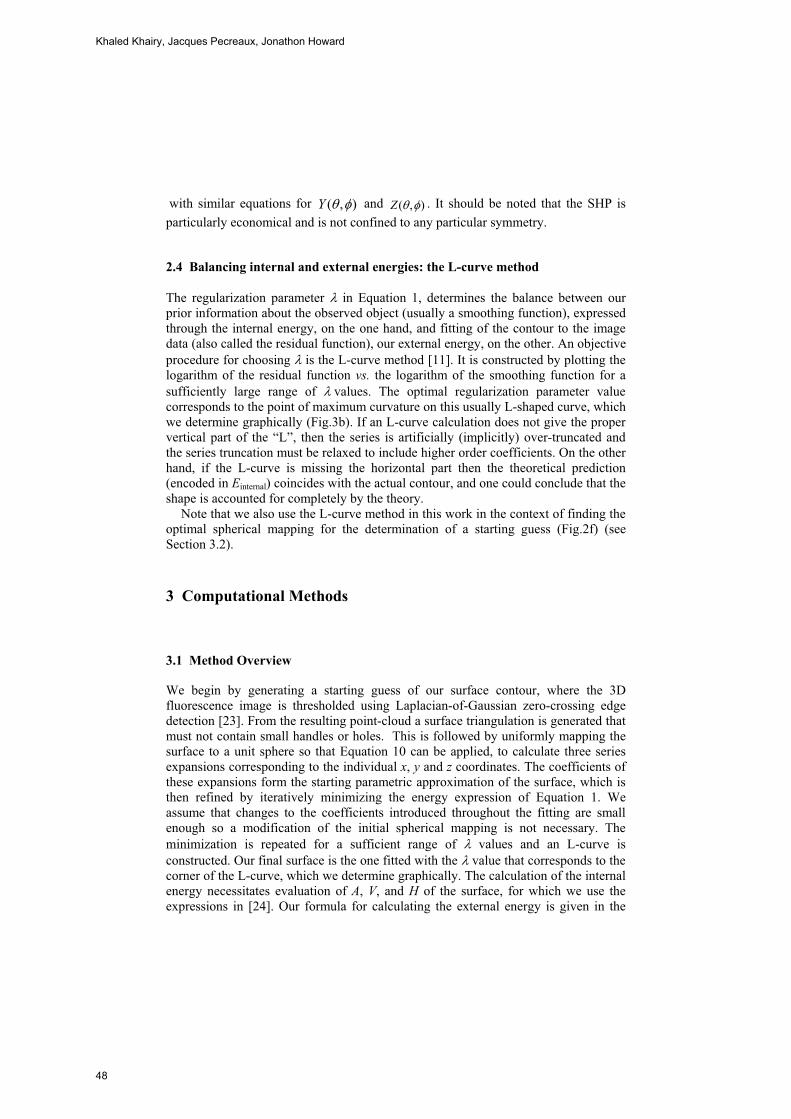
with similar equations for ( , )Y � � and ( , )Z � � . It should be noted that the SHP is particularly economical and is not confined to any particular symmetry.
2.4 Balancing internal and external energies: the L-curve method
The regularization parameter � in Equation 1, determines the balance between our prior information about the observed object (usually a smoothing function), expressed through the internal energy, on the one hand, and fitting of the contour to the image data (also called the residual function), our external energy, on the other. An objective procedure for choosing � is the L-curve method [11]. It is constructed by plotting the logarithm of the residual function vs. the logarithm of the smoothing function for a sufficiently large range of ��values. The optimal regularization parameter value corresponds to the point of maximum curvature on this usually L-shaped curve, which we determine graphically (Fig.3b). If an L-curve calculation does not give the proper vertical part of the “L”, then the series is artificially (implicitly) over-truncated and the series truncation must be relaxed to include higher order coefficients. On the other hand, if the L-curve is missing the horizontal part then the theoretical prediction (encoded in Einternal) coincides with the actual contour, and one could conclude that the shape is accounted for completely by the theory.
Note that we also use the L-curve method in this work in the context of finding the optimal spherical mapping for the determination of a starting guess (Fig.2f) (see Section 3.2).
3 Computational Methods
3.1 Method Overview
We begin by generating a starting guess of our surface contour, where the 3D fluorescence image is thresholded using Laplacian-of-Gaussian zero-crossing edge detection [23]. From the resulting point-cloud a surface triangulation is generated that must not contain small handles or holes. This is followed by uniformly mapping the surface to a unit sphere so that Equation 10 can be applied, to calculate three series expansions corresponding to the individual x, y and z coordinates. The coefficients of these expansions form the starting parametric approximation of the surface, which is then refined by iteratively minimizing the energy expression of Equation 1. We assume that changes to the coefficients introduced throughout the fitting are small enough so a modification of the initial spherical mapping is not necessary. The minimization is repeated for a sufficient range of � values and an L-curve is constructed. Our final surface is the one fitted with the � value that corresponds to the corner of the L-curve, which we determine graphically. The calculation of the internal energy necessitates evaluation of A, V, and H of the surface, for which we use the expressions in [24]. Our formula for calculating the external energy is given in the
Khaled Khairy, Jacques Pecreaux, Jonathon Howard
48
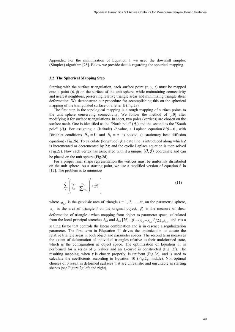
Appendix. For the minimization of Equation 1 we used the downhill simplex (Simplex) algorithm [25]. Below we provide details regarding the spherical mapping.
3.2 The Spherical Mapping Step
Starting with the surface triangulation, each surface point (x, y, z) must be mapped onto a point (����) on the surface of the unit sphere, while maintaining connectivity and nearest neighbors, preserving relative triangle areas and minimizing triangle shear deformation. We demonstrate our procedure for accomplishing this on the spherical mapping of the triangulated surface of a letter E (Fig.2a).
The first step in the topological mapping is a rough mapping of surface points to the unit sphere conserving connectivity. We follow the method of [10] after modifying it for surface triangulations. In short, two poles (vertices) are chosen on the surface mesh. One is identified as the "North pole" (�N) and the second as the "South pole" (�S). For assigning a (latitude) � value, a Laplace equation 2 0�� � , with Dirichlet conditions N 0� � and S� � is solved, (a stationary heat diffusion equation) (Fig.2b). To calculate (longitude) �, a date line is introduced along which �is incremented or decremented by 2 , and the cyclic Laplace equation is then solved (Fig.2c). Now each vertex has associated with it a unique ( , )� � coordinate and can be placed on the unit sphere (Fig.2d).
For a proper final shape representation the vertices must be uniformly distributed on the unit sphere. As a starting point, we use a modified version of equation 6 in [12]. The problem is to minimize
2
2p, o,
o,4
mi i
ii i
i
a aa
!
" #" #$ %$ % �$ %$ %$ %$ %& '& '
� � (11)
where p,ia is the geodesic area of triangle i = 1, 2, …, m, on the parametric sphere,
o,ia is the area of triangle i on the original object, i! is the measure of shear deformation of triangle i when mapping from object to parameter space, calculated from the local principal stretches �i�1 and �i�2 [26], 2
,1 ,2 ,1 ,2( ) 2i i i i i! � � � �� , and is a scaling factor that controls the linear combination and is in essence a regularization parameter. The first term in Edquation 11 drives the optimization to equate the relative triangle areas in both object and parameter spaces. The second term measures the extent of deformation of individual triangles relative to their undeformed state, which is the configuration in object space. The optimization of Equation 11 is performed for a series of � values and an L-curve is constructed (Fig. 2f). The resulting mapping, when is chosen properly, is uniform (Fig.2e), and is used to calculate the coefficients according to Equation 10 (Fig.2g middle). Non-optimal choices of result in deformed surfaces that are unrealistic and unsuitable as starting shapes (see Figure 2g left and right).
Spherical Harmonics 3D Active Contours for Membrane Bilayer- Bound Surfaces
49
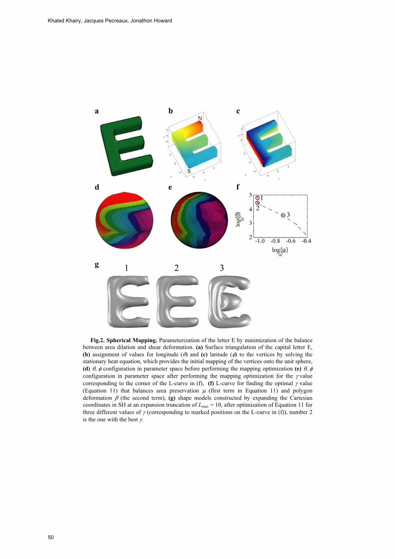
Fig.2. Spherical Mapping. Parameterization of the letter E by minimization of the balance between area dilation and shear deformation. (a) Surface triangulation of the capital letter E, (b) assignment of values for longitude (�) and (c) latitude (�) to the vertices by solving the stationary heat equation, which provides the initial mapping of the vertices onto the unit sphere, (d) �,�� configuration in parameter space before performing the mapping optimization (e) �,��configuration in parameter space after performing the mapping optimization for the �valuecorresponding to the corner of the L-curve in (f), (f) L-curve for finding the optimal value (Equation 11) that balances area preservation ( (first term in Equation 11) and polygon deformation ! (the second term), (g) shape models constructed by expanding the Cartesian coordinates in SH at an expansion truncation of Lmax = 10, after optimization of Equation 11 for three different values of (corresponding to marked positions on the L-curve in (f)), number 2 is the one with the best .
Khaled Khairy, Jacques Pecreaux, Jonathon Howard
50
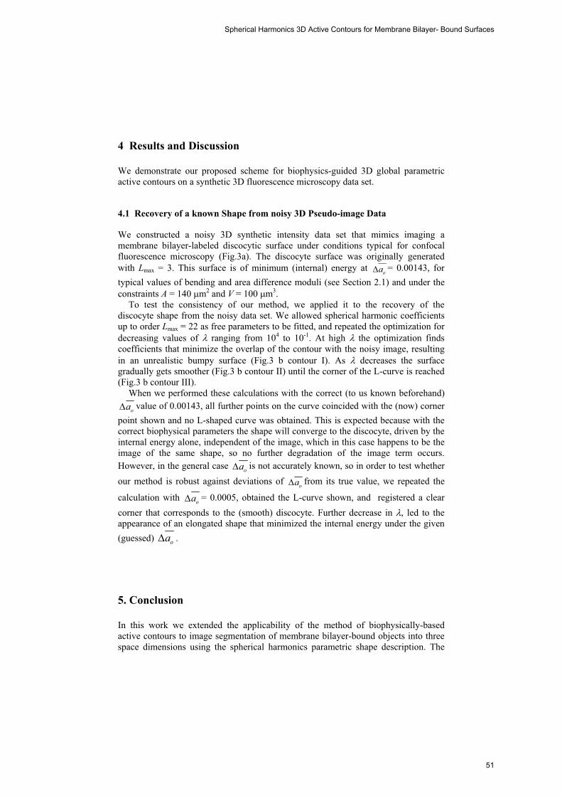
4 Results and Discussion
We demonstrate our proposed scheme for biophysics-guided 3D global parametric active contours on a synthetic 3D fluorescence microscopy data set.
4.1 Recovery of a known Shape from noisy 3D Pseudo-image Data
We constructed a noisy 3D synthetic intensity data set that mimics imaging a membrane bilayer-labeled discocytic surface under conditions typical for confocal fluorescence microscopy (Fig.3a). The discocyte surface was originally generated with Lmax = 3. This surface is of minimum (internal) energy at
oa� = 0.00143, for typical values of bending and area difference moduli (see Section 2.1) and under the constraints A = 140 (m2 and V = 100 (m3.
To test the consistency of our method, we applied it to the recovery of the discocyte shape from the noisy data set. We allowed spherical harmonic coefficients up to order Lmax = 22 as free parameters to be fitted, and repeated the optimization for decreasing values of � ranging from 104 to 10-1. At high � the optimization finds coefficients that minimize the overlap of the contour with the noisy image, resulting in an unrealistic bumpy surface (Fig.3 b contour I). As � decreases the surface gradually gets smoother (Fig.3 b contour II) until the corner of the L-curve is reached (Fig.3 b contour III).
When we performed these calculations with the correct (to us known beforehand)
oa� value of 0.00143, all further points on the curve coincided with the (now) corner point shown and no L-shaped curve was obtained. This is expected because with the correct biophysical parameters the shape will converge to the discocyte, driven by the internal energy alone, independent of the image, which in this case happens to be the image of the same shape, so no further degradation of the image term occurs. However, in the general case oa� is not accurately known, so in order to test whether our method is robust against deviations of oa� from its true value, we repeated the
calculation with oa� = 0.0005, obtained the L-curve shown, and registered a clear corner that corresponds to the (smooth) discocyte. Further decrease in �, led to the appearance of an elongated shape that minimized the internal energy under the given (guessed) oa� .
5. Conclusion
In this work we extended the applicability of the method of biophysically-based active contours to image segmentation of membrane bilayer-bound objects into three space dimensions using the spherical harmonics parametric shape description. The
Spherical Harmonics 3D Active Contours for Membrane Bilayer- Bound Surfaces
51
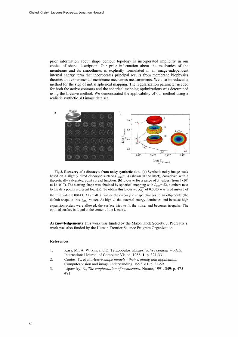
prior information about shape contour topology is incorporated implicitly in our choice of shape description. Our prior information about the mechanics of the membrane and its smoothness is explicitly formulated in an image-independent internal energy term that incorporates principal results from membrane biophysics theories and experimental membrane mechanics measurements. We also introduced a method for the step of initial spherical mapping. The regularization parameter needed for both the active contours and the spherical mapping optimizations was determined using the L-curve method. We demonstrated the applicability of our method using a realistic synthetic 3D image data set.
Fig.3. Recovery of a discocyte from noisy synthetic data. (a) Synthetic noisy image stack based on a slightly tilted discocyte surface (Lmax= 3) (shown in the inset), convolved with a theoretically calculated point spread function. (b) L-curve for a range of � values (from 1x10⁴
to 1x10-1.0). The starting shape was obtained by spherical mapping with Lmax= 22, numbers next to the data points represent log10(�). To obtain this L-curve,
oa� of 0.0005 was used instead of
the true value 0.00143. At small �� values the discocytic shape changes to an elliptocyte (the default shape at this
oa� value). At high �� the external energy dominates and because high expansion orders were allowed, the surface tries to fit the noise, and becomes irregular. The optimal surface is found at the corner of the L-curve.
Acknowledgements This work was funded by the Max-Planck Society. J. Pecreaux’s work was also funded by the Human Frontier Science Program Organization.
References
1. Kass, M., A. Witkin, and D. Terzopoulos, Snakes: active contour models.International Journal of Computer Vision, 1988. 1: p. 321-331.
2. Cootes, T., et al., Active shape models - their training and application.Computer vision and image understanding, 1995. 61: p. 38-59.
3. Lipowsky, R., The conformation of membranes. Nature, 1991. 349: p. 475-481.
Khaled Khairy, Jacques Pecreaux, Jonathon Howard
52

4. Waugh, R. and R. Bauserman, Physical measurements of bilayer-skeletal separation forces. Ann Biomed Eng, 1995. 23(3): p. 308-21.
5. Strey, H., M. Peterson, and E. Sackmann, Measurement of erythrocyte membrane elasticity by flicker eigenmode decomposition. Biophys J, 1995. 69(2): p. 478-88.
6. Scheffer, L., et al., Atomic force pulling: probing the local elasticity of the cell membrane. European Biophysics Journal, 2001. 30(2): p. 83-90.
7. Lim, H.W.G., M. Wortis, and R. Mukhopadhyay, Stomatocyte-discocyte-echinocyte sequence of the human red blood cell: evidence for the bilayer- couple hypothesis from membrane mechanics. Proc Natl Acad Sci USA, 2002. 99(26): p. 16766-9.
8. Doebereiner, H.G., et al., Mapping vesicle shapes into the phase diagram: A comparison of experiment and theory. Phys. Rev. E, 1997. 55(5): p. 4458-74.
9. Pecreaux, J., C. Zimmer, and J. Olivo-Marin. Biophysical Active Contours for Cell Tracking I: Tension and Bending. in ICIP 2006. 2006. Atlanta, USA.
10. Brechbühler, C., G. Gerig, and O. Kuebler, Parametrization of closed surfaces for 3-D shape description. Comput Vision Image Und, 1995. 61(2): p. 154-170.
11. Hansen, P.C., Rank-deficient and discrete ill-posed problems: numerical aspects of linear inversion. 1997, Philadelphia: SIAM.
12. Quicken, M., et al. Parameterization of Closed Surfaces for Parametric Surface Description. in IEEE Computer Society Conference on Computer Vision and Pattern Recognition CVPR 2000. 2000: IEEE Computer Society.
13. Shen, L. and F. Makedon, Spherical mapping for processing of 3D closed surfaces. Image and vision computing, 2006. 24: p. 743-761.
14. Deuling, H.J. and W. Helfrich, Red blood cell shapes as explained on the basis of curvature elasticity. Biophys J, 1976. 16(8): p. 861-8.
15. Sheetz, M.P. and S.J. Singer, Biological membranes as bilayer couples. Proc Natl Acad Sci USA, 1974. 71: p. 4457-4461.
16. Seifert, U., K. Berndl, and R. Lipowsky, Shape transformations of vesicles: Phase diagram for spontaneous- curvature and bilayer-coupling models.Phys Rev A, 1991. 44(2): p. 1182-1202.
17. Heinrich, V., S. Svetina, and B. Zeks, Non-Axisymmetric Vesicle Shapes in a Generalized Bilayer-Couple Model and the Transition between Oblate and Prolate Axisymmetric Shapes. Phys Rev E, 1993. 48(4): p. 3112-3123.
18. Miao, L., et al., Budding transitions of fluid-bilayer vesicles: The effect of area-difference elasticity. Phys Rev E, 1994. 49(6): p. 5389-5407.
19. Mukhopadhyay, R., H.W.G. Lim, and M. Wortis, Echinocyte shapes: bending, stretching, and shear determine spicule shape and spacing.Biophys J, 2002. 82(4): p. 1756-72.
20. Chan, T.F. and L.A. Vese, Active Contours without edges. IEEE Transactions on image processing, 2001. 10(2): p. 266-277.
21. Mumford, D. and J. Shah, Optimal Approximations by Piecewise Smooth Functions and Associated Variational-Problems. Communications on Pure and Applied Mathematics, 1989. 42(5): p. 577-685.
Spherical Harmonics 3D Active Contours for Membrane Bilayer- Bound Surfaces
53

22. Hobson, E.W., The theory of spherical and ellipsoidal harmonics. 1955, New York: Chelsea.
23. Marr, D. and E.C. Hildreth, Theory of edge detection. Proc R Soc Lond Ser B, 1980. 207: p. 187-217.
24. Julicher, F., Die Morphologie von Vesikeln. 1993, University of Cologne. p. 131.
25. Nelder, J.A. and R. Mead, A simplex method for function minimization.Comput J, 1965. 7: p. 308.
26. Evans, E.A. and R. Skalak, Mechanics and Thermodynamics of Biomembranes. 1980, Boca Raton, FL: CRC.
Appendix: Calculation of Eexternal
In analogy with electrostatics, one can write an “electric” field inE�
and outE�
corresponding to a distribution of charge 2in( )I c and 2
out( )I c . Using the Gauss theorem,
2external in in out out out
surface image surface
. ( ) .E E dN I c dV E dN� �� � � � � �
(A-1)
where S SdN� )
* *� +
* *
� is the local surface normal.
This approach would necessitate a careful and precise solution of the Poisson equations for the potential from which inE
� and outE
�are derived. Such a treatment is
beyond the scope of this paper, so for the sake of practicality we compute the value of the image at the contour positions by an integration of the functional derivative of the external energy,
externalin in out out
surface surface
div divE E dN E dNS
, � �,
� � � � �
(A-2)
This only requires the computation of the surface normals using the image value on the surface only, which makes the computation more efficient.
Khaled Khairy, Jacques Pecreaux, Jonathon Howard
54
Modelling Cerebral Cortical Folding
Guangqiang Geng1,2, Leigh Johnston1,3, Edwin Yan4, David Walker5 and GaryEgan1,6
1 Howard Florey Institute2 Graduate School of Biomedical Engineering, University of New South Wales
3 Dept. of Electrical & Electronic Engineering, University of Melbourne4 National Trauma Research Institute, Alfred Hospital
5 Dept. of Physiology, Monash University6 Centre for Neuroscience, University of Melbourne, Australia
Abstract. Understanding the biomechanical mechanisms by which thecerebral cortex folds is a fundamental problem in neuroscience. Cur-rent mathematical models of cortical folding do not include three dimen-sional geometry of developing brains extracted from experimental data.We present a biomechanical model which integrates 3D information ex-tracted from MRI scans of fetal lamb brains at a series of developmentalstages as an initial stage for the computation of cortical folding, andwhich utilises Diffusion Tensor Imaging (DTI) measurements of whitematter fibre directions as a cue to the tension forces thought to regulatefolding. We simulated the structures that result from different loadingsand constraints, and compared the simulated with the actual geometry ofthe developing brain. This work is a proof of principle that finite elementmodels and DTI can be combined to create a biologically meaningfulmodel of the cortical folding process common to higher order mammals.
1 Introduction
The cerebral cortex covers most of the superficial part of the mammalian brain.Folding of the cerebral cortex in human and higher mammals such as the baboonand macaque monkey is related to higher intelligence, such that the greater thedegree of cortical folding, the more intelligent the species [1]. During the initialstages of brain development in the human embryo, a smooth cortex forms by cellmigration from subcortical structures. At the fifth or sixth month of gestation,the cortex begins to fold, forming the gyri (outward folds) and sulci (inwardfolds) from this stage until after birth [2]. The cortical folding increases thesurface area of the cortex relative to the brain volume, thought to maintain aproportional increase of the cortical surface area during significant growth phasesof the cortical volume [3].
Mathematical models have been proposed to investigate the biomechanismsof cortical folding, for improved understanding of the genesis of neurological dis-orders that result in abnormal cortical folding, such as Down’s syndrome [4] andlissencephaly, in which the brain folds are less numerous and smaller than nor-mal folds [3]. These modelling studies simulate cortical folding via mathematical
55

formulation of mechanisms including elasticity and plasticity of the cortex [5, 6],differential growth of cortical layers [3], limitation of the growth by the skull andwhite matter fibres [6], and modulation of tangential neuron migration by chem-ical activation and inhibition [7]. No model of the 3D geometry of the developingcerebral cortex, however, has yet been integrated with experimental data.
Current mathematical models initialise the shape of the cortex prior to fold-ing with artificial geometries such as a closed ring [5], a flat sheet [3], or a 1Dcurve [6]. In addition, most models have no direct extension to 3D [5–7]. Further-more, the resultant simulated geometries are either compared only visually withtrue cortical folding [7], or are quantitatively evaluated, but without comparisonto a real cerebral cortex [5].
In order to understand the regulation of cortical folding by biomechanicalfactors including the 3D developing cortical geometry and white matter fibretension forces, for which no experimental data are available from direct mea-surement, we propose a 3D biomechanical finite element model that integratesexperimental data via Magnetic Resonance Imaging (MRI).
(a) (b)
(c) (d)
Fig. 1. Slices of T2-weighted MRI data for fetal sheep brains at a) 70 b) 90 c) 110 andd) 130 days gestation.
High-resolution MRI data are acquired for a set of fetal lamb brains at 70, 90,110 and 130 days of gestation. As evident in Fig. 1, the surface of the 70 day brainis smooth with only a few shallow dimples. The greatest increase in the numberof sulci occurs between 70 and 90 days gestation, as demonstrated in Fig. 2.For that reason, this study focuses on modelling the geometric deformation of acortical region between 70 and 90 days gestation. The geometry of a smooth 70day cortical region is extracted from the MRI data. The deformation of this initialshape is computed via a dynamic solid stress-strain model, and is subsequentlycompared with the true 90 day brain.
56

We integrate experimental MRI data by using white matter fibre anisotropy,as measured by Diffusion Tensor Imaging (DTI) [8], as a cue to tension appliedbetween subcortical structures and the interior cortical surface. White matterfibre tension has been proposed by Van Essen to be a critical factor in theregulation of cortical folding [9].
70 90 110 130 1500
5
10
15
20
25
30
35
40
45
50
Num
ber
ofSulc
i
Time of Gestation (day)
Fig. 2. Number of sulci in the fetal lamb brain as a function of gestational age.
2 Methods
2.1 Preparation of Fetal Lamb Brains
Fetal sheep brains are extracted at the relevant gestational time points. Eachfetus is perfused transcardially with 500-1000ml of heparinized saline accordingto the size of the fetus, followed by the same volume of 4% Paraformaldehyde(PFA). The brain is subsequently removed from the fetus, and is placed in 4%PFA at least 48 hours before the MRI scan.
2.2 Acquisition of MRI Data
A Bruker Biospec 4.7T animal MRI scanner is used. T2-weighted and diffusionweighted imaging (DWI) data are acquired for each of the brains via a multi-slice multiecho sequence and a standard DTI sequence. Coronal slices of 1mmthickness with in-plane resolution of 0.258× 0.258 mm2 are acquired perpendic-ular to the anterior-posterior commissure line. For the 70 day brain, the imagingmatrix is 128 × 128 × 30 (Fig. 3a), while the imaging matrix is 256 × 256 × 45(Fig. 3b) for the 90 day brain due to the increased brain size. TE = 50ms forboth brains, TR = 4s and 10s for the 70 and 90 day brains, respectively. Twelve-direction DWI data are acquired following the T2-weighted scan with the samematrix size, spatial resolution, TE and TR, with a b-value of 1000 s/mm2 forboth brains.
Modelling Cerebral Cortical Folding
57
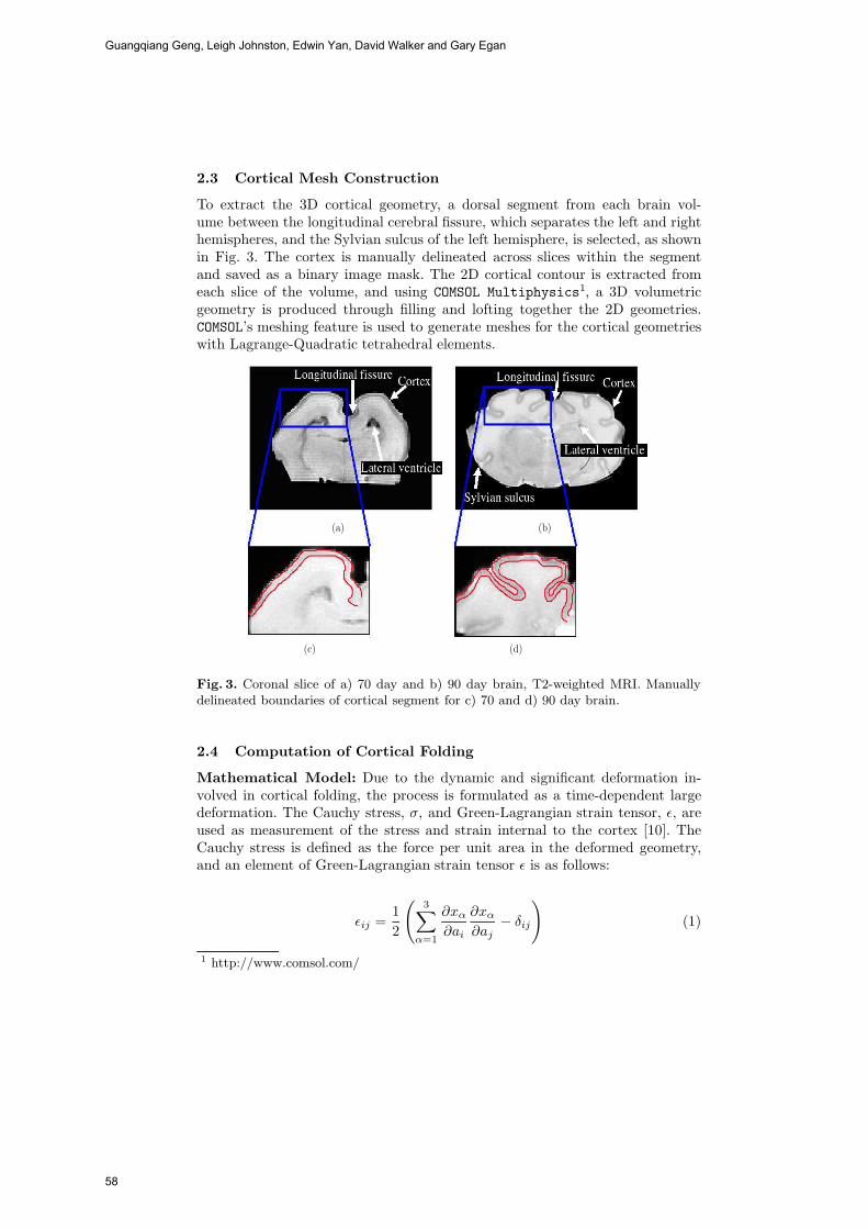
2.3 Cortical Mesh Construction
To extract the 3D cortical geometry, a dorsal segment from each brain vol-ume between the longitudinal cerebral fissure, which separates the left and righthemispheres, and the Sylvian sulcus of the left hemisphere, is selected, as shownin Fig. 3. The cortex is manually delineated across slices within the segmentand saved as a binary image mask. The 2D cortical contour is extracted fromeach slice of the volume, and using COMSOL Multiphysics1, a 3D volumetricgeometry is produced through filling and lofting together the 2D geometries.COMSOL’s meshing feature is used to generate meshes for the cortical geometrieswith Lagrange-Quadratic tetrahedral elements.
(a) (b)
(c) (d)
Fig. 3. Coronal slice of a) 70 day and b) 90 day brain, T2-weighted MRI. Manuallydelineated boundaries of cortical segment for c) 70 and d) 90 day brain.
2.4 Computation of Cortical Folding
Mathematical Model: Due to the dynamic and significant deformation in-volved in cortical folding, the process is formulated as a time-dependent largedeformation. The Cauchy stress, σ, and Green-Lagrangian strain tensor, ε, areused as measurement of the stress and strain internal to the cortex [10]. TheCauchy stress is defined as the force per unit area in the deformed geometry,and an element of Green-Lagrangian strain tensor ε is as follows:
εij =12
(3∑
α=1
∂xα
∂ai
∂xα
∂aj− δij
)(1)
1 http://www.comsol.com/
Guangqiang Geng, Leigh Johnston, Edwin Yan, David Walker and Gary Egan
58
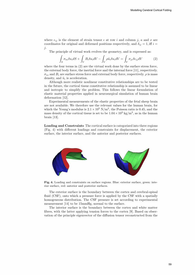
where εij is the element of strain tensor ε at row i and column j, a and x arecoordinates for original and deformed positions respectively, and δij = 1, iff i =j.
The principle of virtual work evolves the geometry, and is expressed as:∫S
σniδuidS +∫V
BiδuidV −
∫V
ρuiδuidV =∫V
σjiδεijdV (2)
where the four terms in (2) are the virtual work done by the surface stress force,the external body force, the inertial force and the internal force [11], respectively.σni and Bi are surface stress force and external body force, respectively. ρ is massdensity, and ui is acceleration.
Although more realistic nonlinear constitutive relationships are to be testedin the future, the cortical tissue constitutive relationship is assumed to be linearand isotropic to simplify the problem. This follows the linear formulation ofelastic material properties applied in neurosurgical simulation of human braindeformation [12].
Experimental measurements of the elastic properties of the fetal sheep brainare not available. We therefore use the relevant values for the human brain, forwhich the Young’s modulus is 2.1× 10⁵ N/m2, the Poisson ratio is 0.45, and themass density of the cortical tissue is set to be 1.04×10³ kg/m3, as in the humanbrain [13].
Loading and Constraints The cortical surface is categorized into three regions(Fig. 4) with different loadings and constraints for displacement, the exteriorsurface, the interior surface, and the anterior and posterior surfaces.
Fig. 4. Loading and constraints on surface regions. Blue: exterior surface, green: inte-rior surface, red: anterior and posterior surfaces.
The exterior surface is the boundary between the cortex and cerebral-spinalfluid (CSF), onto which a pressure force is applied by the CSF with a spatiallyhomogeneous distribution. The CSF pressure is set according to experimentalmeasurement [14] to be 15mmHg, normal to the surface.
The interior surface is the boundary between the cortex and white matterfibres, with the latter applying tension forces to the cortex [9]. Based on obser-vation of the principle eigenvector of the diffusion tensor reconstructed from the
Modelling Cerebral Cortical Folding
59
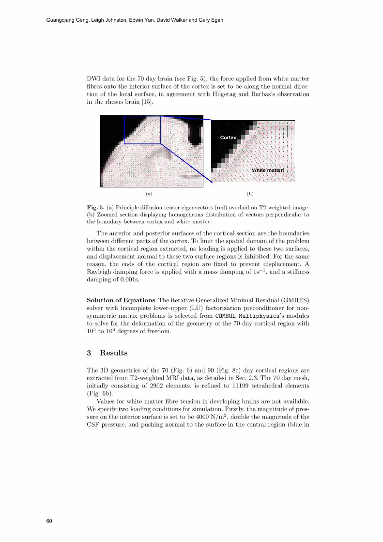
DWI data for the 70 day brain (see Fig. 5), the force applied from white matterfibres onto the interior surface of the cortex is set to be along the normal direc-tion of the local surface, in agreement with Hilgetag and Barbas’s observationin the rhesus brain [15].
(a) (b)
Fig. 5. (a) Principle diffusion tensor eigenvectors (red) overlaid on T2-weighted image.(b) Zoomed section displaying homogeneous distribution of vectors perpendicular tothe boundary between cortex and white matter.
The anterior and posterior surfaces of the cortical section are the boundariesbetween different parts of the cortex. To limit the spatial domain of the problemwithin the cortical region extracted, no loading is applied to these two surfaces,and displacement normal to these two surface regions is inhibited. For the samereason, the ends of the cortical region are fixed to prevent displacement. ARayleigh damping force is applied with a mass damping of 1s−1, and a stiffnessdamping of 0.001s.
Solution of Equations The iterative Generalized Minimal Residual (GMRES)solver with incomplete lower-upper (LU) factorization preconditioner for non-symmetric matrix problems is selected from COMSOL Multiphysics’s modulesto solve for the deformation of the geometry of the 70 day cortical region with105 to 106 degrees of freedom.
3 Results
The 3D geometries of the 70 (Fig. 6) and 90 (Fig. 8c) day cortical regions areextracted from T2-weighted MRI data, as detailed in Sec. 2.3. The 70 day mesh,initially consisting of 2902 elements, is refined to 11199 tetrahedral elements(Fig. 6b).
Values for white matter fibre tension in developing brains are not available.We specify two loading conditions for simulation. Firstly, the magnitude of pres-sure on the interior surface is set to be 4000 N/m2, double the magnitude of theCSF pressure, and pushing normal to the surface in the central region (blue in
Guangqiang Geng, Leigh Johnston, Edwin Yan, David Walker and Gary Egan
60
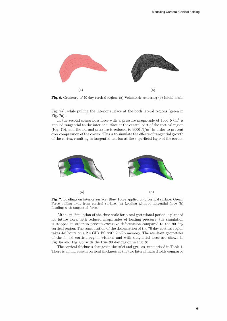
(a) (b)
Fig. 6. Geometry of 70 day cortical region. (a) Volumetric rendering (b) Initial mesh.
Fig. 7a), while pulling the interior surface at the both lateral regions (green inFig. 7a).
In the second scenario, a force with a pressure magnitude of 1000 N/m2 isapplied tangential to the interior surface at the central part of the cortical region(Fig. 7b), and the normal pressure is reduced to 3000 N/m2 in order to preventover compression of the cortex. This is to simulate the effects of tangential growthof the cortex, resulting in tangential tension at the superficial layer of the cortex.
(a) (b)
Fig. 7. Loadings on interior surface. Blue: Force applied onto cortical surface. Green:Force pulling away from cortical surface. (a) Loading without tangential force (b)Loading with tangential force.
Although simulation of the time scale for a real gestational period is plannedfor future work with reduced magnitudes of loading pressure, the simulationis stopped in order to prevent excessive deformation compared to the 90 daycortical region. The computation of the deformation of the 70 day cortical regiontakes 4-8 hours on a 2.4 GHz PC with 2.5Gb memory. The resultant geometriesof the folded cortical region without and with tangential force are shown inFig. 8a and Fig. 8b, with the true 90 day region in Fig. 8c.
The cortical thickness changes in the sulci and gyri, as summarised in Table 1.There is an increase in cortical thickness at the two lateral inward folds compared
Modelling Cerebral Cortical Folding
61

(a) (b) (c)
Fig. 8. (a) Simulated geometry without tangential force. (b) Simulated geometry withtangential force. (c) 90 day geometry extracted from T2-weighted MRI data.
Gyri Sulci Ratioleft right mean (gyri/sulci)
No tangential force 1.01 1.29 1.63 1.46 0.69
With tangential force 1.00 1.15 1.63 1.39 0.72
90 day geometry 1.07 1.81 1.90 1.86 0.58
Table 1. Cortical thickness in gyri and sulci (mm)
to a homogeneous cortical thickness of 1.09 mm within the 70 day cortical region.This is due to the compression of the central part of the cortex by the CSFpressure from the exterior surface and the normal pushing force from the interiorsurface. At the two lateral inward folds, the normal force pulls the interior surfaceof the cortex away from its exterior surface.
The application of a tangential force on the interior surface at the centralpart of the cortical region results in more realistic geometry (Fig. 8b) with abroader gyral section as in the real 90 day cortical region. The cortical thicknessin a scenario without tangential force is compared with that of a scenario witha tangential force. There is larger change in cortical thickness for the simulationwith tangential force compared to the result without tangential force (Table 1)both in gyri and sulci. Hilgetag and Barbas [15] suggested this to be a resultof the normal compression onto the deep layers of the cortex, induced by thetangential tension applied on the superficial layer of the cortex, verified in thissimulation with tangential force. As is shown in Table 1, the cortical thicknessin simulation results either with or without tangential force is less than that ofthe 90 day cortical geometry in both gyri and sulci. This is due to the limitationthat cortical thickness growth is not simulated in this study.
4 Discussion and Conclusions
This study simulates the cortical folding of an intial 3D geometry directly ex-tracted from MR volumetric data, for a fetal lamb brain at 70 days of gestation.This is immediately an improvement to existing theoretical 1D and 2D models ofcortical folding that contain no experimental data. The physical properties and
Guangqiang Geng, Leigh Johnston, Edwin Yan, David Walker and Gary Egan
62

displacement constraints for the brain tissue and CSF pressure are nominated upaccording to experimental human brain measurements. Our biologically mean-ingful mechanical model simulates the tension applied by white matter fibres,based on DTI data, to regulate cortical folding as proposed by Van Essen [9].
The 3D geometry resultant from the computation of cortical deformation isqualitatively similar to the geometry directly extracted from the MR volumet-ric data for the folded cortical region in the 90 day brain. The results of thissimulation verify as a proof of principle that cortical folding can be simulatedin 3D with an initial geometry directly extracted from a developing brain. Thecomputed geometric change simulates the cortical folding both outward and in-ward. The simulated change of cortical thickness agrees with the observationand measurement on the real 90 day cortical region. Application of tangentialtension at the interior surface of the cortical region results in broader outwardfolding as well as a further decrease in cortical thickness, which results in thesimulated geometry being more similar to the actual cortical region. However,the increase of the thickness and tangential size of the cortex is not formulatedin the current study, which leads to difference between the simulated and actualgeometries.
We are currently working on a number of improvements to this preliminaryinvestigation. Firstly, the nonlinear formulation of the constitutive properties ofbrain tissue, which are more realistic for soft tissues [10, 16, 17] and have beenimplemented in simulation of brain deformation for image registration requiredby neurosurgery [18] as well as for modelling the deformation of other soft tis-sues [19–21]. Secondly, the mechanical force applied on the interior surface of thecortex can be quantitatively integrated from DTI data as an improvement to thecurrent qualitative formulation. In this approach, the orientations of the princi-ple eigenvectors of the diffusion tensors will provide the direction of the whitematter fibre tension, and the anisotropy of the diffusion will be proportional tothe magnitude of the tension force. In addition, the full cortex will be considered,rather than the present section, and the brains of subsequent gestational ageswill be integrated, for a complete picture of the folding pattern.
References
1. Buettner-Janusch, J.: Evolutionary and genetic biology of primates: Volume 1.Academic Press, New York (1963)
2. Ottoson, D.: Physiology of the nervous system. The Macmillan Press, London andBasingstoke (1983)
3. Richman, D.P., Stewart, R.M., Hutchinson, J.W., Caviness, J.V.S.: Developmentalmodel of brain convolutional development. Science 189(4196) (1975) 18–21
4. Venita, J.: Pathology in an infant with Down’s syndrome and Tuberous Sclerosis.Pediatrics Neurology 15 (1996) 57–59
5. Toro, R., Burnod, Y.: A morphogenetic model for the development of corticalconvolutions. Cerebral Cortex 15 (2005) 1900–1913
6. Raghavan, R., Lawton, W., Ranjan, S., Viswannathan, R.: A continuum mechanics-based model for cortical growth. Journal of Theoretical Biology 187 (1997) 285–296
Modelling Cerebral Cortical Folding
63

7. Cartwright, J.: Labyrinthine Turing pattern formation in the cerebral cortex.Journal of Theoretical Biology 217 (2002) 97–103
8. Basser, P.J., Mattiello, J., LeBihan, D.: MR diffusion tensor spectroscopy andimaging. Biophysical Journal 66 (1994) 259–267
9. Van Essen, D.C.: A tension-based theory of morphogenesis and compact wiring inthe central nervous system. Nature 385 (1997) 313–318
10. Fung, Y.C.: Biomechanics: Mechanical properties of living tissues. 2 edn. Springer-Verlag, New York (1993)
11. Boresi, A.P., Chong, K.P.: Elasticity in engineering mechanics. Elsevier, New York(1987)
12. Warfield, S.K., Ferrant, M., Gallez, X., Nabavi, A., Jolesz, F.A., Kikinis, R.: Real-time biomechanical simulation of volumetric brain deformation for image guidedneurosurgery. In: SC 2000: High Performance Networking and Computing Confer-ence; 2000 Nov 4–10; Dallas, USA. (2000) 230:1–16
13. Gao, C., Tay, F.E.H., Nowinski, W.L.: Modelling of the human brain with detailedanatomy for numerical simulation of surgical interventions. Journal of Physics:Conference Series 34 (2006) 985–989
14. Neville, L., Egan, R.A.: Frequency and amplitude of elevation of cerebrospinal fluidresting pressure by the valsalva maneuver. Canadian Journal of Ophthalmology40 (2005) 775–777
15. Hilgetag, L.C., Barbas, H.: Developmental mechanics of the primate cerebral cor-tex. Anatomy and Embryology 210 (2005) 411–417
16. Spencer, A.J.M.: Continuum Mechanics. Longman, New York (1980)17. Malvern, L.E. In: Introduction to the mechanics of a continuous medium. Prentice-
Hall (1969) 27318. Hagemann, A., Rohr, K.: Biomechanical modeling of the human head for physically
based, nonrigid image registration. IEEE Transaction on medical imaging 18(10)(1999) 875–884
19. Pathmanathan, P., Gavaghan, D., Whiteley, J., Brady, S.M., Nash, M., Nielsen,P., Rajagopal, V.: Predicting tumour location by simulating large deformations ofthe breast using a 3D finite element model and nonlinear elasticity. In: MICCAI.(2004) pp. 217–224
20. Nash, M.P., Hunter, P.J.: Computational mechanics of the heart. Journal ofElasticity 61 (2000) 113–141
21. Fernandez, J.W., Hunter, P.J.: An anatomically based patient-specific finite ele-ment model of patella articulation: towards a diagnostic tool. Biomechanical Modelin Mechanobiology 4 (2005) 20–38
Guangqiang Geng, Leigh Johnston, Edwin Yan, David Walker and Gary Egan
64
Suite of finite element algorithms for accurate computation of soft tissue deformation for surgical
simulation
Grand Roman Joldes, Adam Wittek, Karol Miller
Intelligent Systems for Medicine Lab., The University of Western Australia, 35 Stirling Highway, Crawley, WA 6009, AUSTRALIA
{grandj, adwit, kmiller}@mech.uwa.edu.au
Abstract. Real time computation of soft tissue deformation is important for the usage of augmented reality devices and for providing haptic feedback during operation or surgeon training. This requires algorithms that are both fast and ac-curate and can handle material and geometric nonlinearities. A combination of such algorithms is presented in this paper, starting with the finite element for-mulation and integration scheme used and addressing common problems such as hourglass control and locking. The computation example presented proves that by using these algorithms real time computations becomes possible without having to sacrifice the accuracy of the results.
Keywords: non-locking tetrahedron, hourglass control, real time computations, Total Lagrangian formulation, explicit time integration
1 Introduction
Systems using augmented reality for image guided surgery are important tools that can help surgeons to improve the accuracy and limit the adverse effects of surgery. The existing imaging technology, such as MRI, provides good quality pre-operative images that can be used in such a system. These images can be analyzed and regis-tered on the real organs so that the surgeon can visualize the targeted area while the procedure is progressing.
Another area where fast computational algorithms are required is the Computer In-tegrated Surgery (CIS) systems that must provide haptic feedback to the surgeon. Various haptic interfaces for medical simulation are especially useful for training of minimally invasive procedures (laparoscopy/interventional radiology) and remote surgery using teleoperators. These systems must compute the interaction force be-tween the robotic tool and the tissue and provide it to the surgeon at frequencies in the area of 500 Hz [1].
Biomechanical models are used for solving the haptic feedback problems using the finite element method, but many such models are simplified in order to decrease the computational effort, e.g. they consider only infinitesimal deformations and/or linear material laws. These simplifications have great influence on the accuracy of the ob-
65

tained results in a finite element analysis, inducing significant errors [2-4]. Therefore material law and geometric non-linearity must be considered when a solution method is chosen.
There are three methods of reducing the computation time: improvement of the al-gorithms, usage of faster hardware or usage of parallel computing. We will concen-trate on the first method, as the usage of faster hardware is limited by the existing technology and the usage of parallel computing leads to more complex and more ex-pensive hardware and software systems.
The paper is organized as follows: the proposed algorithms are presented in section 2, a computational example demonstrates the efficiency of these algorithms in section 3 and the conclusions are presented in section 4.
2 Finite element algorithms
When designing a finite element solution method there are many aspects that must be considered, such as the formulation used (Total or Updated Lagrangian), time integra-tion scheme and the type of elements used for constructing the mesh. We will discuss these aspects in the following section.
2.1 Total Lagrangian Explicit integration
Various spatial discretisation schemes are possible while using the finite element method [5]. The algorithms used by the great majority of commercial finite element programs use the Updated Lagrangian formulation, where all variables are referred to the current (i.e. from the end of the previous time step) configuration of the system (Ansys [6], ABAQUS [7], ADINA [8], LS Dyna [9], etc.). The advantage of this ap-proach is the simplicity of incremental strain description. The disadvantage is that all derivatives with respect to spatial coordinates must be recomputed in each time step, because the reference configuration is changing. The reason for this choice is histori-cal – at the time of solver development the memory was expensive and caused more problems than the actual speed of computations. The first key idea in the finite ele-ment algorithms development was to use the Total Lagrangian formulation of finite element method, where all variables are referred to the original configuration of the system. Second-Piola Kirchoff stress and Green strain are used. The decisive advan-tage of this formulation is that all derivatives with respect to spatial coordinates are calculated with respect to original configuration and therefore can be precomputed. The proposed stress and strain measures are appropriate for handling geometric non-liniarities (finite deformations).
The usage of Total Lagrangian explicit integration for simulating physically realis-tic deformations was also proposed in [10]. A method for decreasing the computation time when using non-linear elasticity was presented in [11], but it only works for tet-rahedral meshes and special elastic material laws.
Because biological tissues behavior can be described in general using hyper-elastic or hyper-visco-elastic models [12], the usage of the Total Lagrangian formulation also
Grand Roman Joldes, Adam Wittek, Karol Miller
66

leads to a simplification of material law implementation as these material models can be easily described using the deformation gradient.
The integration of equilibrium equations in time domain can be done using either implicit or explicit methods [13-15]. The most commonly used implicit integration methods, such as the Newmarks’ constant acceleration method, are unconditionally stable. This implies that their time step is limited only by the convergence/accuracy considerations. However, the implicit methods require solution of set of non-linear algebraic equations at each time step. Furthermore, iterations need to be performed for each time step of implicit integration to control the error and prevent divergence. Therefore, the number of numerical operations per each time step can be three orders of magnitude larger than for explicit integration [13].
On the other hand, in explicit methods, such as a central difference method, treat-ment of non-linearities is very straightforward and no iterations are required. By using a lumped (diagonalised) mass matrix, the equations of motion can be decoupled and no system of equations must be solved. Computations are done at the element level eliminating the need for assembling the stiffness matrix of the entire model. Thus, computational cost of each time step and internal memory requirements are substan-tially smaller for explicit than for implicit integration. There is no need for iterations anywhere in the algorithm. These features make explicit integration suitable for real time applications.
However, the explicit methods are only conditionally stable. Normally a severe re-striction on the time step size has to be included in order to receive satisfactory simu-lation results. Stiffness of soft tissue is very low [16-18]: e.g. stiffness of brain is about eight orders of magnitude lower than that of steel. Since the maximum time step allowed for stability is (roughly speaking) inversely proportional to the square root of Young’s modulus divided by the mass density, it is possible to conduct simulations of brain deformation with much longer time steps than in typical dynamic simulations in engineering. A detailed description of the Total Lagrange Explicit Dynamics [TLED] algorithm is presented in [19].
2.2 Elements used in the mesh
Because of the computation time requirement, the mesh must be constructed using low order elements that are not computationally intensive, such as the linear tetrahe-dron or the linear under-integrated hexahedron. The standard formulation of the tetra-hedral element exhibits volumetric locking [14], especially in case of soft tissues such as the brain, that are modeled as almost incompressible materials [17]. Therefore hexahedral elements are preferred.
Many algorithms are now available for fast and accurate automatic mesh genera-tion using tetrahedral elements, but not for automatic hexahedral mesh generation [20-22]. This is one reason why many authors proposed the usage of tetrahedral meshes for their models [23-26]. In order to automate the simulation process, mixed meshes (having both hexahedral and tetrahedral elements) with predominantly hexa-hedral elements are the most convenient.
The under-integrated hexahedral elements require the usage of an hourglass control algorithm in order to eliminate the zero energy modes which arise from the one-point
Suite of finite element algorithms for accurate computation of soft tissue deformation for surgical simulation
67
integration [27]. Special algorithms for handling hourglass control for the hexahedral elements and to reduce locking of the tetrahedral elements must be implemented.
2.3 Hourglass control
One of the most popular and powerful hourglass control algorithms, that is currently available in many commercial software finite element packages, is the one proposed by Flanagan and Belytschko in [27]. This method is applicable for hexahedral ele-ments with arbitrary geometry undergoing large deformations.
Starting from that algorithm proposed by Flanagan and Belytschko we could show that the Total Lagrangian formulation is also recommended from the point of view of efficient hourglass control implementation, as many quantities involved can be pre-computed. We have shown in [28] that the hourglass control forces for each element can be computed (in matrix form) as:
u��F tTHgt k 0000 = (1)
where k is a constant that depends on the element geometry and material proper-ties, Y is the matrix of hourglass shape vectors and u is the matrix of current dis-placements. The notation from [14] is used, where the left superscript represents the current time and the left subscript represents the time of the reference configuration, which is 0 for Total Lagrangian. In (1) all quantities except u are constant and can be pre-computed, making the hourglass control mechanism very efficient.
2.4 Improved tetrahedral elements
There are a number of improved (non-locking) linear tetrahedral elements already proposed by different authors [29-31]. These formulations are either much more com-putationally intensive than the standard formulation or the volumetric locking control mechanism depends on material properties (e.g. bulk modulus), making harder the in-terfacing of different materials. Our volumetric lock control mechanism is computa-tionally inexpensive and depends solely on kinematic variables.
As defined in [30], the nodal Jacobian is the ratio between the current and initial nodal volumes. The nodal volume is computed as a sum of fractions of the surround-ing element volumes.
Using the nodal Jacobians, an average Jacobian can be computed for each element. Because the element Jacobian is equal to the determinant of the element deformation gradient, we define a modified element deformation gradient that has the same iso-choric part as the normal deformation gradient, but the volumetric part is modified so that its determinant (and therefore the volumetric deformation) is equal to the average element Jacobian.
The computation of the nodal forces (or stiffness matrix) can now be done in the usual manner, but using the modified deformation gradient instead of the normal de-formation gradient for defining the strains. This way there is no need for computing the isochoric and deviatoric components of the internal forces separately, and the ex-isting material law can be used [32].
Grand Roman Joldes, Adam Wittek, Karol Miller
68
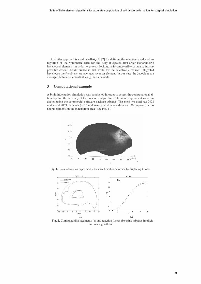
A similar approach is used in ABAQUS [7] for defining the selectively reduced in-tegration of the volumetric term for the fully integrated first-order isoparametric hexahedral elements, in order to prevent locking in incompressible or nearly incom-pressible cases. The difference is that while for the selectively reduced integrated hexahedra the Jacobians are averaged over an element, in our case the Jacobians are averaged between elements sharing the same node.
3 Computational example
A brain indentation simulation was conducted in order to assess the computational ef-ficiency and the accuracy of the presented algorithms. The same experiment was con-ducted using the commercial software package Abaqus. The mesh we used has 2428 nodes and 2059 elements (2023 under-integrated hexahedron and 36 improved tetra-hedral elements in the indentation area - see Fig. 1).
Fig. 1. Brain indentation experiment – the mixed mesh is deformed by displacing 4 nodes
a) b)
Fig. 2. Computed displacements (a) and reaction forces (b) using Abaqus implicit and our algorithms
Suite of finite element algorithms for accurate computation of soft tissue deformation for surgical simulation
69
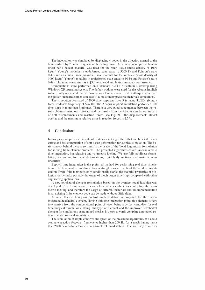
The indentation was simulated by displacing 4 nodes in the direction normal to the brain surface by 20 mm using a smooth loading curve. An almost incompressible non-linear neo-Hookean material was used for the brain tissue (mass density of 1000 kg/m3, Young’s modulus in undeformed state equal to 3000 Pa and Poisson’s ratio 0.49) and an almost incompressible linear material for the ventricle (mass density of 1000 kg/m3, Young’s modulus in undeformed state equal to 10 Pa and Poisson’s ratio 0.49). The same constraints as in [33] were used and brain symmetry was assumed.
Computations were performed on a standard 3.2 GHz Pentium 4 desktop using Windows XP operating system. The default options were used for the Abaqus implicit solver. Fully integrated mixed formulation elements were used in Abaqus, which are the golden standard elements in case of almost incompressible materials simulations.
The simulation consisted of 2000 time steps and took 3.8s using TLED, giving a force feedback frequency of 526 Hz. The Abaqus implicit simulation performed 100 time steps in more than 5 minutes. There is a very good concordance between the re-sults obtained using our software and the results from the Abaqus simulation, in case of both displacements and reaction forces (see Fig. 2) – the displacements almost overlap and the maximum relative error in reaction forces is 2.5%.
4 Conclusions
In this paper we presented a suite of finite element algorithms that can be used for ac-curate and fast computation of soft tissue deformation for surgical simulation. The ba-sic concept behind these algorithms is the usage of the Total Lagrangian formulation for solving finite element problems. The presented algorithms cover issues related to time integration, hourglassing and volumetric locking. We use fully nonlinear formu-lation, accounting for large deformations, rigid body motions and material non-linearities.
Explicit time integration is the preferred method for performing real time simula-tions. The treatment of non-linearities is straightforward, without the need of any it-eration. Even if the method is only conditionally stable, the material properties of bio-logical tissue make possible the usage of much larger time steps compared with other engineering applications.
A new tetrahedral element formulation based on the average nodal Jacobian was developed. This formulation uses only kinematic variables for controlling the volu-metric locking, and therefore the usage of different materials and the implementation in an existing finite element code can be made without difficulties.
A very efficient hourglass control implementation is proposed for the under-integrated hexahedral element. Having only one integration point, this element is very inexpensive from the computational point of view, being a perfect candidate for real time surgical simulations. Using this type of element and the improved tetrahedral element for simulations using mixed meshes is a step towards complete automated pa-tient specific surgical simulation.
The simulation example confirms the speed of the presented algorithms. We could compute reaction forces at frequencies higher than 500 Hz for a mesh having more than 2000 hexahedral elements on a simple PC workstation. The accuracy of our re-
Grand Roman Joldes, Adam Wittek, Karol Miller
70

sults was demonstrated by comparing them with the results of a similar simulation done using much more complex elements in the commercial finite element software Abaqus.
Acknowledgements: The first author was an IPRS scholar in Australia during the completion of this research. The financial support of the Australian Research Council (Grant No. DP0343112, DP0664534 and LX0560460) is gratefully acknowledged.
References
1. DiMaio, S.P. and Salcudean, S.E.: Interactive Simulation of Needle Insertion Models. IEEE Trans. on Biomedical Engineering. (2005) 52(7)
2. Carey, G.F.: A Unified Approach to Three Finite Element Theories for Geometric Nonlinearity. Journal of Computer Methods in Applied Mechan-ics and Engineering (1974) 4(1): p. 69-79
3. Martin, H.C. and Carey, G.F.: Introduction to Finite Element Analysis: The-ory and Application. McGraw-Hill Book Co., New York (1973)
4. Oden, J.T. and Carey, G.F.: Finite Elements: Special Problems in Solid Me-chanics. Prentice-Hall, (1983)
5. Belytschko, T.: An Overview of Semidiscretization and Time Integration Procedures, in Computational Methods for Transient Analysis, Editor: T. Be-lytschko and T.J.R. Hughes (1983) North-Holland: Amsterdam. p. 1-66
6. http://www.ansys.com/services/documentation, ANSYS documentation, Ac-cessed: 18/10/2005
7. ABAQUS: ABAQUS Theory Manual, Version 5.8. Hibbitt, Karlsson & Sorensen, Inc., (1998)
8. www.adina.com, ADINA home page, Accessed: 22/11/2005 9. Hallquist, J.O.: LS-DYNA Theory Manual. Livermore Software Technology
Corporation, Livermore, California 94551 (2005) 10. Zhuang, Y. and Canny, J.: Real-time Simulation of Physically Realistic
Global Deformation. IEEE Vis'99 (1999) San Francisco, California 11. Picinbono, G., Delingette, H., and Ayache, N.: Non-linear anisotropic elas-
ticity for real-time surgery simulation. Graphical Models (2003) 65: p. 305-321
12. Fung, Y.C.: Biomechanics. Mechanical Properties of Living Tissues. Second ed. Springer-Verlag, New York (1993)
13. Belytschko, T.: A survey of numerical methods and computer programs for dynamic structural analysis. Nuclear Engineering and Design (1976) 37: p. 23-34
14. Bathe, K.-J.: Finite Element Procedures. Prentice-Hall, New Jersey (1996) 15. Crisfield, M.A.: Non-linear dynamics, in Non-linear Finite Element Analysis
of Solids and Structures, (1998) John Wiley & Sons: Chichester. p. 447-489 16. Miller, K. and Chinzei, K.: Constitutive modelling of brain tissue; Experi-
ment and Theory. Journal of Biomechanics (1997) 30(11/12): p. 1115-1121 17. Miller, K.: Biomechanics of Brain for Computer Integrated Surgery. Publish-
ing House of Warsaw University of Technology, Warsaw (2002)
Suite of finite element algorithms for accurate computation of soft tissue deformation for surgical simulation
71
18. Miller, K. and Chinzei, K.: Mechanical properties of brain tissue in tension. Journal of Biomechanics (2002) 35: p. 483-490
19. Miller, K., et al.: Total Lagrangian Explicit Dynamics Finite Element Algo-rithm for Computing Soft Tissue Deformation. Communications in Numeri-cal Methods in Engineering (2007) 23: p. 121-134
20. Owen, S.J.: A Survey of Unstructured Mesh Generation Technology. 7th In-ternational Meshing Roundtable (1998) Dearborn, Michigan, USA
21. Viceconti, M. and Taddei, F.: Automatic generation of finite element meshes from computed tomography data. Critical Reviews in Biomedical Engineer-ing (2003) 31(1): p. 27-72
22. Owen, S.J.: Hex-dominant mesh generation using 3D constrained triangula-tion. Computer-Aided Design (2001) 33: p. 211-220
23. Ferrant, M., et al.: Deformable Modeling for Characterizing Biomedical Shape Changes. Discrete Geometry for Computer Imagery: 9th International Conference (2000) Uppsala, Sweden: Springer-Verlag GmbH
24. Ferrant, M., et al.: Serial registration of intraoperative MR images of the brain. Medical Image Analysis (2002) 6(4): p. 337-359
25. Clatz, O., et al.: Patient Specific Biomechanical Model of the Brain: Appli-cation to Parkinson's disease procedure. International Symposium on Surgery Simulation and Soft Tissue Modeling (IS4TM'03) (2003) Juan-les-Pins, France: Springer-Verlag
26. Warfield, S.K., et al.: Real-time registration of volumetric brain MRI by biomechanical simulation of deformation during image guided surgery. Computing and Visualization in Science (2002) 5: p. 3-11
27. Flanagan, D.P. and Belytschko, T.: A uniform strain hexahedron and quadri-lateral with orthogonal hourglass control. International Journal for Numerical Methods in Engineering (1981) 17: p. 679-706
28. Joldes, G.R., Wittek, A., and Miller, K.: Efficient Hourglass Control Imple-mentation for the Uniform Strain Hexahedron Using the Total Lagrangian Formulation. Communications in Numerical Methods in Engineering (2007) Submitted, under review
29. Bonet, J. and Burton, A.J.: A simple averaged nodal pressure tetrahedral element for incompressible and nearly incompressible dynamic explicit ap-plications. Communications in Numerical Methods in Engineering (1998) 14: p. 437-449
30. Bonet, J., Marriott, H., and Hassan, O.: An averaged nodal deformation gra-dient linear tetrahedral element for large strain explicit dynamic applications. Communications in Numerical Methods in Engineering (2001) 17: p. 551-561
31. Zienkiewicz, O.C., et al.: Triangles and Tetrahedra in Explicit Dynamic Codes for Solids. International Journal for Numerical Methods in Engineer-ing (1998) 43: p. 565-583
32. Joldes, G.R., Wittek, A., and Miller, K.: Improved Linear Tetrahedral Ele-ment for Surgical Simulation. Computational Biomechanics for Medicine - MICCAI 2006 Workshop Proceedings (2006) Copenhagen, Denmark
Grand Roman Joldes, Adam Wittek, Karol Miller
72

33. Wittek, A., et al.: Computing reaction forces on surgical tools for robotic neurosurgery and surgical simulation. Australasian Conference on Robotics and Automation ACRA (2004) Canberra, Australia
Suite of finite element algorithms for accurate computation of soft tissue deformation for surgical simulation
73
Finite Element Simulation of the Beating Heartfor Image-Guided Robotic Cardiac Surgery
Philip Pratt1, Fernando Bello1, Eddie Edwards1, and Daniel Rueckert2
1 Department of Biosurgery and Surgical Technology2 Visual Image Processing, Department of ComputingImperial College of Science, Technology and Medicine
London, United [email protected]
Abstract. An interactive finite element simulation of the beating heartis described in which the intrinsic motion is implied from preoperative4D tomographic scan data. The equations of motion are reversed, suchthat given changes in node displacements over time, the node forces thatproduce those changes are recovered. Subsequently, these forces are re-solved from the global coordinate system into systems local to each meshelement. Therefore, at each simulation time step, the collection of nodeforces can be expressed as simple weighted sums of current node posi-tions. Importantly, this facilitates the combination of extrinsic forces suchas those due to tool-tissue interactions, changes in the relative directionin which gravity acts, and effects due to insufflation of the thoracic cav-ity and left lung deflation. Through the development of an image-guidedcoronary artery bypass application of the daVinci tele-manipulator sys-tem, the method has been applied initially to volumetric images of apneumatically-operated beating heart phantom.
1 Introduction
During the past decade, technical innovations have led to considerable advancesin cardiac surgery. One such advance is the introduction of minimally invasivetechniques. In particular, robotic tele-manipulator systems have made totallyendoscopic coronary artery bypass (TECAB) a reality. But reductions in inci-sion sizes and post-operative recovery times have seen corresponding increasesin technical difficulty and durations of the procedures. This is partly because thesurgeon cannot touch and palpate tissues directly, thereby making it more diffi-cult to locate key anatomical structures beneath the tissue surface, and partlybecause of the limited field of vision afforded by the endoscopic cameras. Imageguidance, using tomographic scan data acquired preoperatively, is one approachwhich addresses these limitations [1, 2]. A key requirement for image guidancein TECAB is the availability of 2D-3D registration techniques that can accu-rately process complex motion patterns and deformations. In addition to theintrinsic cardiac and respiratory motion, one must take into account tool-tissueinteractions, effects due to left lung deflation, insufflation of the thoracic cavity,and the patient’s position on the operating table relative to that adopted forpreoperative scans.
74
This paper introduces a finite element model where the sequence of nodeforces required to produce intrinsic motion is recovered. These forces are resolvedfrom the global coordinate system to be functions of their local geometry. In thisway, their application is consistent with large-scale deformations and rotationsand, more importantly, other extrinsic forces can be combined. The techniquecould be said to bring time-varying 3D scan data to life, such that it can beinteracted with and not only observed.
Several relevant ideas have been put forward recently. In particular, thiswork builds on the image-guidance approach of Wang [3] and Wang et al. [4],who simulate tool-tissue interactions between a phantom heart and da Vinciendowrist instrument, integrating 3D geometry reconstructed from preoperativeCT/MRI scans with a non-linear finite element model. The heart is nominallystatic, and has no intrinsic beating motion. Nakao [5] describes a model of thepulsating aorta, driven by cyclic changes in aortic blood pressure, which canbe palpated by virtual tools in the context of a cardiac surgery simulation.Szalpa et al. [6] have developed an image guidance system for minimally-invasivecardiac surgery, whereby endoscopic images of a beating heart phantom areoverlaid with CT images of the same. To reconstruct arbitrary phases of thecardiac cycle, non-linear free-form deformations are used to warp a high-qualityimage of the diastolic phase. Similarly, Wierzbicki et al. [7] create a dynamicepicardial surface mesh from a sequence of CT images. Chandrashekara et al.[8] have developed a non-rigid registration technique, based on Catmull-Clarksubdivision lattices, to track the motion of the left ventricle in tagged MR images.Various finite element simulations have been described in which deformations areknown a priori. Specifically, Kruggel and Tittgemeyer [9] use an inverse finiteelement model to derive a force field given an observed deformation of the brain.Kauer [10] also uses an inverse model to calibrate the properties of a visco-elasticmaterial given experimental pressure data and resulting tissue deformations.
2 Methods
The tetrahedral finite element mesh comprises N nodes, and therefore has amaximum 3N degrees of freedom. In general, zero or more of these freedoms willbe restrained. Following the notation in [11], restrained freedoms are specifiedby the node freedom array rjk, where the coordinate axes are labelled j = 0, 1, 2and the nodes are numbered k = 0, 1, . . . , N −1. Non-negative entries in thearray label the D degrees of freedom in the mesh. The initial mesh geometry isspecified by the global coordinate array gjk. The equations of motion for a linearelastic solid are expressed in terms of the D displacements from the initial meshconfiguration, i.e. u = [u0 u1 . . . uD−1]�. Thus, they can be written as
Mu + Cu + Ku = f (1)
where M is the mass matrix, C is the viscous damping matrix, K is the stiffnessmatrix, f is the time-varying vector of applied forces, and u, u and u are thedisplacement, velocity and acceleration vectors, respectively. Rayleigh dampingis assumed, i.e. C = αmM + αkK.
Finite Element Simulation of the Beating Heart for Image-Guided Robotic Cardiac Surgery
75
2.1 Average Acceleration Integration
If Δt denotes the duration of each simulation time step, then using the Newmarkfamily of integration methods [12], the discretised equations of motion take thefollowing form. One can employ the implicit average acceleration method bysetting β = 1/4 and γ = 1/2.
ai = 1βΔt2 ui + 1
βΔt ui + ( 12β − 1)ui
bi = γβΔtui − (1 − γ
β )ui − (1 − γ2β )Δtui
ui+1 =[K + γ
βΔtC + 1βΔt2 M
]−1
(fi + Mai + Cbi)
ui+1 = γβΔtui+1 − bi
ui+1 = 1βΔt2 ui+1 − ai
(2)
Given initial displacements, velocities and accelerations, the equations are iter-ated in the order listed above at each time step. The linear system is solvedusing Cholesky decomposition and back-substitution. The positions pjki of eachnode k at any particular time step i are given by the following expression.
pjki ={gjk + urjki if rjk ≥ 0gjk otherwise (3)
2.2 Recovering Forces from Displacements
The motion is assumed to be cyclic, spanning a total of T time steps. Successorand predecessor functions of the time index i are defined as follows.
next(i) ={i+ 1 if i < T − 10 otherwise prev(i) =
{i− 1 if i > 0T − 1 otherwise (4)
Using these definitions, two-sided finite difference approximations to the firstand second-order derivatives of the displacement vector yield the following ex-pressions for velocity and acceleration.
ui = 12Δt
(unext(i) − uprev(i)
)ui = 1
Δt2
(unext(i) − 2ui + uprev(i)
)(5)
These are used to compute the initial conditions u0 and u0 from the knowndisplacements. By inverting the displacement update step in (2) as follows, onecan compute the discretised applied forces from known changes in displacement.Then by construction, if one were to solve the equations of motion and applythese forces at the appropriate times, one would recover the original cyclic motionexactly and indefinitely.
fi =[K +
γ
βΔtC +
1βΔt2
M]ui+1 − Mai − Cbi (6)
Philip Pratt, Fernando Bello, Eddie Edwards, and Daniel Rueckert
76
2.3 Forces as Functions of Local Geometry
In order to combine intrinsic and extrinsic forces, the former must be expressednot in the global coordinate system, but for each node in terms of its local sur-rounding geometry. With the introduction of extrinsic forces, the geometry maydeviate from the original cyclic motion through potentially large-scale deforma-tions and rotations. By resolving intrinsic forces locally, they are made to act inthe appropriate direction in conjunction with any extrinsically induced motion.
The intrinsic force acting on a particular node in the mesh is assumed tooriginate from the finite elements which contain that node. Indeed, an approxi-mation is made whereby the force receives an equal contribution from each suchelement. For a given element at each point in time, the edge vectors from thenode in question to the other three nodes in that element define a local basisin terms of which that element’s fraction of the node force can be expressed.This amounts to equating the force to a weighted sum of those edge vectors andsolving for the weights. Subsequently, the weights are further accumulated overthe node’s other parent elements, ultimately building a set of weights that linksall the intrinsic forces to the geometry of the entire mesh.
Labelled with coordinate indices j, components hjki of the node forces aremapped onto those applicable to each degree of freedom fi = [f0
i f1i . . . f
D−1i ]�
by the node freedom array.
hjki ={frjki if rjk ≥ 0
0 otherwise (7)
Figure 1 (left) depicts at time step i a typical node k with its recovered force,and the five surrounding elements e0, ..., e4 to which it belongs. In general, anode will be common to Mk elements. Figure 1 (middle) illustrates the firstelement e0, and the three edge vectors bj0i , bj1i and bj2i which, with the nodeitself, define the geometry of the element at that instant. In order to express therequired fraction of the force in terms of local mesh geometry, its componentsin the global coordinate system are equated to weighted combinations of theseedge vectors as follows.⎡
⎣ b00i b01i b02ib10i b11i b12ib20i b21i b22i
⎤⎦
⎡⎣w0
i
w1i
w2i
⎤⎦ =
1Mk
⎡⎣h
j0i
hj1ihj2i
⎤⎦ (8)
The weights are determined by direct inversion of the left-hand-side matrix. Byaccumulating contributions from each element containing the node, writing edgevectors in terms of node positions, incorporating the node freedom array, andconsidering all nodes, the total intrinsic force for each degree of freedom l canbe expressed as
f li =∑j
∑k
vjkli pjki (9)
which lends itself particularly well to efficient implementation. Thus, in the ab-sence of extrinsic forces and together with the finite element model, the sequence
Finite Element Simulation of the Beating Heart for Image-Guided Robotic Cardiac Surgery
77

of aggregate weights vjkli completely determines the cyclic motion of the mesh.At each point in time, intrinsic forces are determined by local geometry only.The connectivity of the mesh dictates that many of the weights will be zero.
In order to ensure that the magnitudes of the intrinsic forces f li , expressedas functions of position, do not give rise to simulation instability, the forces arenormalised at each time step to have the same magnitude as those implied fromthe original motion where no extrinsic forces are present.
Fig. 1. Force resolution using local geometry and a typical external face
2.4 Tool-Tissue Interactions
Tool-tissue interactions are combined in the simulation by means of a simple in-strument model, in which the end effector is taken to be a line segment. Barycen-tric coordinates returned by the collision detection algorithm upon detection of aface intersection are used to distribute an additional applied force appropriatelyover its three nodes. The magnitude of the force is proportional to the depth ofsegment penetration.
2.5 Insufflation
The mesh comprises a set of external triangular faces upon which pressurisedinsufflation gas can exert force. Figure 1 (right) shows one such face at a certaininstant in time i, comprising nodes pj0i , pj1i and pj2i . It is assumed that theforce due to insufflation pressure acts in a direction normal to the face, with amagnitude proportional to its area. The force is distributed uniformly over eachof the face’s three nodes. Viscous and frictional forces acting in other directionsare assumed to be negligible. The face area A and unit normal n are simplefunctions of the node positions. At each simulation time step, insufflation forcesare accumulated over all external faces in the mesh to give the total additionalforce applied to each node.
Philip Pratt, Fernando Bello, Eddie Edwards, and Daniel Rueckert
78
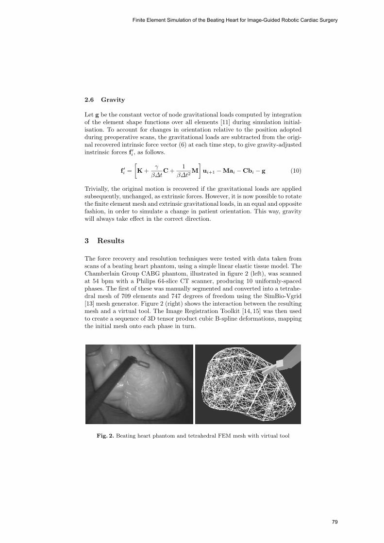
2.6 Gravity
Let g be the constant vector of node gravitational loads computed by integrationof the element shape functions over all elements [11] during simulation initial-isation. To account for changes in orientation relative to the position adoptedduring preoperative scans, the gravitational loads are subtracted from the origi-nal recovered intrinsic force vector (6) at each time step, to give gravity-adjustedinstrinsic forces f ′i , as follows.
f ′i =[K +
γ
βΔtC +
1βΔt2
M]ui+1 − Mai − Cbi − g (10)
Trivially, the original motion is recovered if the gravitational loads are appliedsubsequently, unchanged, as extrinsic forces. However, it is now possible to rotatethe finite element mesh and extrinsic gravitational loads, in an equal and oppositefashion, in order to simulate a change in patient orientation. This way, gravitywill always take effect in the correct direction.
3 Results
The force recovery and resolution techniques were tested with data taken fromscans of a beating heart phantom, using a simple linear elastic tissue model. TheChamberlain Group CABG phantom, illustrated in figure 2 (left), was scannedat 54 bpm with a Philips 64-slice CT scanner, producing 10 uniformly-spacedphases. The first of these was manually segmented and converted into a tetrahe-dral mesh of 709 elements and 747 degrees of freedom using the SimBio-Vgrid[13] mesh generator. Figure 2 (right) shows the interaction between the resultingmesh and a virtual tool. The Image Registration Toolkit [14, 15] was then usedto create a sequence of 3D tensor product cubic B-spline deformations, mappingthe initial mesh onto each phase in turn.
Fig. 2. Beating heart phantom and tetrahedral FEM mesh with virtual tool
Finite Element Simulation of the Beating Heart for Image-Guided Robotic Cardiac Surgery
79
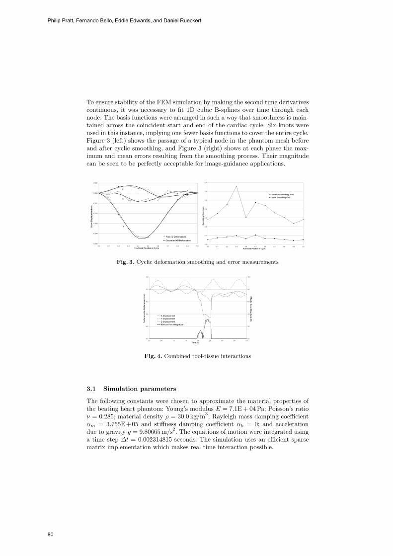
To ensure stability of the FEM simulation by making the second time derivativescontinuous, it was necessary to fit 1D cubic B-splines over time through eachnode. The basis functions were arranged in such a way that smoothness is main-tained across the coincident start and end of the cardiac cycle. Six knots wereused in this instance, implying one fewer basis functions to cover the entire cycle.Figure 3 (left) shows the passage of a typical node in the phantom mesh beforeand after cyclic smoothing, and Figure 3 (right) shows at each phase the max-imum and mean errors resulting from the smoothing process. Their magnitudecan be seen to be perfectly acceptable for image-guidance applications.
Fig. 3. Cyclic deformation smoothing and error measurements
Fig. 4. Combined tool-tissue interactions
3.1 Simulation parameters
The following constants were chosen to approximate the material properties ofthe beating heart phantom: Young’s modulus E = 7.1E + 04Pa; Poisson’s ratioν = 0.285; material density ρ = 30.0 kg/m3; Rayleigh mass damping coefficientαm = 3.755E+05 and stiffness damping coefficient αk = 0; and accelerationdue to gravity g = 9.80665 m/s2. The equations of motion were integrated usinga time step Δt = 0.002314815 seconds. The simulation uses an efficient sparsematrix implementation which makes real time interaction possible.
Philip Pratt, Fernando Bello, Eddie Edwards, and Daniel Rueckert
80
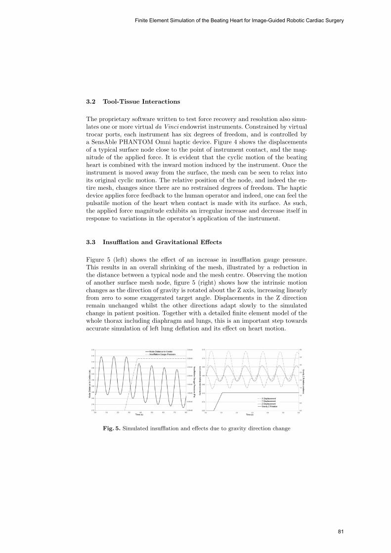
3.2 Tool-Tissue Interactions
The proprietary software written to test force recovery and resolution also simu-lates one or more virtual da Vinci endowrist instruments. Constrained by virtualtrocar ports, each instrument has six degrees of freedom, and is controlled bya SensAble PHANTOM Omni haptic device. Figure 4 shows the displacementsof a typical surface node close to the point of instrument contact, and the mag-nitude of the applied force. It is evident that the cyclic motion of the beatingheart is combined with the inward motion induced by the instrument. Once theinstrument is moved away from the surface, the mesh can be seen to relax intoits original cyclic motion. The relative position of the node, and indeed the en-tire mesh, changes since there are no restrained degrees of freedom. The hapticdevice applies force feedback to the human operator and indeed, one can feel thepulsatile motion of the heart when contact is made with its surface. As such,the applied force magnitude exhibits an irregular increase and decrease itself inresponse to variations in the operator’s application of the instrument.
3.3 Insufflation and Gravitational Effects
Figure 5 (left) shows the effect of an increase in insufflation gauge pressure.This results in an overall shrinking of the mesh, illustrated by a reduction inthe distance between a typical node and the mesh centre. Observing the motionof another surface mesh node, figure 5 (right) shows how the intrinsic motionchanges as the direction of gravity is rotated about the Z axis, increasing linearlyfrom zero to some exaggerated target angle. Displacements in the Z directionremain unchanged whilst the other directions adapt slowly to the simulatedchange in patient position. Together with a detailed finite element model of thewhole thorax including diaphragm and lungs, this is an important step towardsaccurate simulation of left lung deflation and its effect on heart motion.
Fig. 5. Simulated insufflation and effects due to gravity direction change
Finite Element Simulation of the Beating Heart for Image-Guided Robotic Cardiac Surgery
81
4 Conclusion
This paper describes a novel technique for constructing finite element simulationswith cyclical intrinsic motion recovered from 4D tomographic scan data, wherebyextrinsic forces can be combined to produce realistic composite behaviour. Inthe context of an augmented reality application of the da Vinci robotic tele-manipulator system for TECAB, it offers several means by which the accuracyof overlay registration can be improved. Tool-tissue interactions, insufflation andeffects due to gravity and change in patient orientation are combined with thebeating heart. The technique is clearly also applicable to the field of surgicalsimulation and others where, for example, respiratory motion and patient incli-nation must be combined to produce accurate organ deformations, such as thetreatment of liver tumours using robot-assisted RF ablation. Overall accuracyand validity of the technique will be determined by comparing simulation resultsto spatial data recovered from stereo endoscopic video sequences and recordingsof effector positions.
It is also planned to extend the simulation to include non-linear finite elementmodels. Clearly, the linear elastic model defined in (1) is not appropriate ifthe technique were applied to real patient data, but it suffices to illustrate thecentral ideas of force recovery and resolution in the heart phantom case. Whennon-linearities are present, the discretised equations of motion (2) are no longerapplicable. Instead, an iterative scheme, such as the Newton-Raphson methodfor non-linear systems of equations, can be used to solve for the forces requiredto produce known displacements. Typically, the forward integration will alsoinvolve an iterative process [16], ensuring that dynamic equilibrium is restoredat each simulation time step. At each such iteration, the internal forces andmodified stiffness are re-calculated. Further refinements to the simulation willbe made by introducing unequal weights and anisotropy during the local forceresolution process, and by allowing weight interpolation over time, such that thefrequency of cyclic motion can be modified.
Acknowledgements
The Image Registration Toolkit was used under licence from IXICO Ltd.. Theauthors would like to thank staff at St. Mary’s and the Royal Brompton hospitals.
References
1. Chiu, A.M., Dey, D., Drangova, M., Boyd, W.D., Peters, T.M.: 3-D Image Guid-ance for Minimally Invasive Robotic Coronary Artery Bypass. The Heart SurgeryForum 3(3) (2000) 224–231
2. Falk, V., Mourgues, F., Adhami, L., Jacobs, S., Thiele, H., Nitzsche, S., Mohr,F.W., Coste-Maniere, E.: Cardio Navigation: Planning, Simulation, and Aug-mented Reality in Robotic Assisted Endoscopic Bypass Grafting. Annals of Tho-racic Surgery 79(6) (2005) 2040–2047
Philip Pratt, Fernando Bello, Eddie Edwards, and Daniel Rueckert
82

3. Wang, D.A.: Video-Based Augmented Reality For The da Vinci Tele-ManipulatorSystem. PhD thesis, Department of Biosurgery and Surgical Technology, ImperialCollege of Science, Technology and Medicine, University of London (2005)
4. Wang, D.A., Faraci, A., Bello, F., Darzi, A.: Simulating Tele-Manipulator Con-trolled Tool-Tissue Interactions Using a Nonlinear FEM Deformable Model. InWestwood, J.D., et al., eds.: Medicine Meets Virtual Reality 14, IOS Press (2006)565–567
5. Nakao, M.: Cardiac Surgery Simulation with Active Interaction and AdaptivePhysics-Based Modeling. PhD thesis, Department of Social Informatics, GraduateSchool of Informatics, Kyoto University (2003)
6. Szpala, S., Guiraudon, G., Peters, T.: Cardiac Endoscopy Enhanced by DynamicOrgan Modeling for Minimally-Invasive Surgery Guidance. In Ellis, R.E., Pe-ters, T.M., eds.: Medical Image Computing and Computer-Assisted Intervention -MICCAI 2003, Springer (2003) 499–506
7. Wierzbicki, M., Drangova, M., Guiraudon, G., Peters, T.: Validation of dynamicheart models obtained using non-linear registration for virtual reality training,planning, and guidance of minimally invasive cardiac surgeries. Medical ImageAnalysis 8(3) (2004) 387–401
8. Chandrashekara, R., Razavi, R., Mohiaddin, R., Rueckert, D.: Nonrigid imageregistration with subdivision lattices: Application to cardiac MR image analysis.Submitted to Medical Image Analysis (2006)
9. Kruggel, F., Tittgemeyer, M.: Inverse Biomechanical Models of the Brain. InKamm, R., Schmid-Schonbein, G., Athesian, G., Hefzy, M., eds.: Proceedings of the2001 Bioengineering Conference, The American Society of Mechanical Engineers,New York (2001) 837–838
10. Kauer, M.: Inverse Finite Element Characterization of Soft Tissues with AspirationExperiments. PhD thesis, Swiss Federal Institute of Technology, Zurich (2001)
11. Smith, I.M., Griffiths, D.V.: Programming the finite element method. 4th edn.John Wiley and Sons Ltd. (2004)
12. Hughes, T.J.R.: The finite element method: linear static and dynamic finite elementanalysis. Dover Publications, Inc. (2000)
13. Berti, G.: Image-based unstructured 3D mesh generation for medical applica-tions. In Neittaanmaki, P., Rossi, T., Majava, K., Pironneau, O., eds.: Euro-pean Congress on Computational Methods in Applied Sciences and Engineering -ECCOMAS 2004, University of Jyvaskyla, Department of Mathematical Informa-tion Technology (2004)
14. Rueckert, D., Sonoda, L.I., Hayes, C., Hill, D.L.G., Leach, M.O., Hawkes, D.J.:Non-rigid registration using free-form deformations: Application to breast MR im-ages. IEEE Transactions on Medical Imaging 18(8) (1999) 712–721
15. Schnabel, J.A., Rueckert, D., Quist, M., Blackall, J.M., Castellano-Smith, A.D.,Hartkens, T., Penney, G.P., Hall, W.A., Liu, H., Truwit, C.L., Gerritsen, F.A., Hill,D.L.G., Hawkes, D.J.: A generic framework for non-rigid registration based on non-uniform multi-level free-form deformations. In Niessen, W.J., Viergever, M.A., eds.:Medical Image Computing and Computer-Assisted Intervention - MICCAI 2001,Springer (2001) 573–581
16. Reddy, J.N. In: An Introduction to Nonlinear Finite Element Analysis. OxfordUniversity Press (2004) 304–306
Finite Element Simulation of the Beating Heart for Image-Guided Robotic Cardiac Surgery
83
Purely Evidence Based Multiscale Cardiac
Tracking Using Optic Flow
Hans van Assen1, Luc Florack1,�, Avan Suinesiaputra2, Jos Westenberg2, andBart ter Haar Romeny1
1 Biomedical Image Analysis, Dept. Biomedical Engineering, Technical UniversityEindhoven TU/e, Den Dolech 2, 5600 MB Eindhoven, Netherlands
[email protected] http://bmia.bmt.tue.nl2 Div. Image Proc., Dept. Radiology, Leiden Univ. Med. Center, Leiden, Netherlands
Abstract. Heart disease can negatively influence cardiac pump func-tion. To assess cardiac tissue function, a method based on classical opti-cal flow theory applied in the spectral domain is presented. Assumptionof pixel intensity conservation is replaced by assumption of spatial phaseconservation. Simultaneous application to two independent observationsof the same optical flow field removes the necessity of additional con-straints (i.e. flow field smoothness, normal flow) to solve the optical flowconstraint equation (OFCE). Using the 1st order Taylor expansion ofthe OFCE, our system yields not only pixel displacements, but also the1st order differential structure of the displacements (i.e. strains), whichotherwise should be calculated as a post-processing step.Operation at pixel level obviates the need for interpolation of tag lines orsparse flow field representation. Experiments show coherent flow fields ofa human cardiac systole. Comparison with velocity encoded MRI showsa good resemblance.
Key words: optical flow, tracking, heart, tagging, strain, HARP
1 Introduction
Many cardiac diseases have a large influence on the pump function of the cardiacleft ventricle (LV). Valvular aorta stenosis, e.g., impedes blood flow from the leftventricle through the aortic valve into the aorta, thus serving as an obstruc-tion. Furthermore, aorta stenosis influences systolic torsion and diastolic apicaluntwisting [1].Measurements of muscle function are often used as prognostic indicator of successor failure of therapy. SV is one of the well-known indicators used in clinicalpractice for both diagnostic and prognostic purposes. Ejection fraction (EF),which is SV divided by end-diastolic volume, is the most often used functionalparameter in both experimental and clinical studies. Due to a high afterload inaortic stenosis, EF may be reduced even while tissue function may be relatively� The Netherlands Organisation for Scientific Research (NWO) is gratefully acknowl-
edged for financial support.
84
2 H.C. van Assen et al.
normal [2]. This shows that EF as an indirect measure of tissue function may bemisleading. Therefore, it would be better to measure tissue function itself.A method is required that assesses cardiac tissue function both globally and lo-cally and provides new means and criteria for assessment of mechanical dysfunc-tion and to monitor response to treatment [3]. We propose to estimate cardiacfunction from tagged MR [4, 5] spatiotemporal image sequences by classificationof the LV contraction pattern. Towards such an approach, we present a purelyevidence based multiscale method for tissue function assessment from multipletagged image sequences using neither interpolation of tags [6] or flow field [7],nor smoothness assumptions. Our approach follows the original rationale of Hornand Schunck [8], and extended to a multiscale framework by Florack et al. [9],Niessen et al. [10, 11] and Suinesiaputra et al. [12], and of spectral filtering in-troduced by Osman et al. [13]. As opposed to previous methods, however, wedo not invoke any smoothness assumption or other hypothesis for resolving the“aperture problem” (intrinsic flow indeterminacy), but instead base ourselvesentirely on data evidence.In Section 2, we present general background information. In Section 3, we intro-duce optical flow and the way it is used in our proposed method. In Section 3.2,we explain our method, and in Section 4 we show some experimental results.Finally, in Section 5 we discuss results and future directions.
2 Background
2.1 Magnetic Resonance Tagging
In the late 1980s, Zerhouni et al. introduced a method (“tagging”) for visualisingintramyocardial motion by MR imaging [14], later refined to (3D) (C)SPAMM [4,5, 15]. The HARP technique, which employs tagging combined with spectral fil-tering in k-space [13, 16], overcomes tag fading by directly measuring phase in-formation (Fig. 1(b)) of the MR signal (Fig. 1(a)). In 1999, another phase-basedmethod for imaging myocardial function, called DENSE was introduced [17]. Theprinciples behind HARP and DENSE, however, are the same [18]. A third well-known imaging protocol for dynamic analysis is Phase Constrast MRI (PCMRI)[19]. This technique directly measures velocity, which has to be integrated overtime and spatially differentiated to obtain strains, which is far from trivial dueto a limited temporal resolution. Moreover, PCMRI is subject to velocity errors,which propagate during displacement and strain analysis. For a review of motionanalysis MRI protocols, cf. [18].Patterns created with (C)SPAMM are inherent in the tissue, allowing analysisof the local dynamic behaviour of and strains in the LV, while imaging of thecardiac surfaces focuses on wall thickening. Strain analysis is superior to wallthickening analysis to detect wall motion abnormalities [20], since surface-basedapproaches are unable to display disturbances in, e.g., twisting during contrac-tion and relaxation, which have been identified as early signs in pathologies [21].
Purely Evidence Based Multiscale Cardiac Tracking Using Optic Flow
85

Purely Evidence Based Multiscale Cardiac Tracking Using Optic Flow 3
Fig. 1. Left: vertically lined tagged image. Middle: Harmonic phase (HARP) image.Right: Sine of the HARP image.
2.2 Tag Tracking
Tracking with Optical Flow Tracking tags with optical flow methods hasbeen presented before. Niessen et al. [10, 11]used a canine heart from MR cine im-ages and Suinesiaputra et al. [12] tracked human hearts using grid tagging. Bothapplied the multiscale generalisation [9] of the OFCE by Horn and Schunck [8].This method yields one equation and two unknowns in the zeroth-order ap-proximation and four equations with eight unknowns in 1st-order approxima-tion (Sec 3.1). To solve for all unknowns an additional constraint was required.Suinesiaputra et al. formalized the fact that flow components tangential to iso-surfaces (“tangential flow”) cannot be retrieved from data evidence in a “normalflow constraint”. Constraining the flow to underlying image structure, the cal-
culated optical flow does not necessarily correspond to the true optical flow.Dougherty et al. [22] also applied optical flow theory to analyze cardiac motion.They estimate global and local motion in a coarse-to-fine model-based technique.This technique encompasses a Laplacian filter to compensate for intensity andcontrast loss in myocardial tags which violate the basic assumption of constantpoint brightness in optical flow techniques. This technique was compared with asemi-automatic method based on tracking individual tag intersection points [23].The tag intersection points were found by manually thresholding the normalizedcross-correlation result of the tagged MR image with a template of an idealizedtag intersection, and served as input to an interactive active contour model.This technique yields the optical flow field at a sparse set of points in the imagesequence, necessitating an interpolation step to obtain a dense field. Prince andMcVeigh [24] developed an optical flow based method which requires extensiveprior knowledge of the relaxation times T1, T2 and the proton density D0 of themyocardium. The adaptation of this technique by Gupta and Prince [25] stillrequires knowledge of T1 over the image domain.
Tracking with Harmonic Phase (HARP) A different tracking methodbased on filtering in the Fourier domain (or k-space) is the Harmonic Phase(HARP) technique [13]. HARP involves spectral bandpass filtering and subse-quently tracking phases in the angle image of the inverse Fourier transformedfilter result. The HARP method serves as a basis for our optical flow basedtracking technique, and is therefore further explained in Section 3.
Hans van Assen, Luc Florack, Avan Suinesiaputra, Jos Westenberg, and Bart ter Haar Romeny
86

4 H.C. van Assen et al.
3 Methods3.1 Optical Flow
The classical approach to optical flow extraction [8] departs from an optical flowconstraint equation (OFCE) that is intrinsically underdetermined, since flowcomponents tangential to iso-surfaces (“tangential flow”) cannot be retrievedfrom data evidence. This indeterminacy is commonly referred to as the “aper-ture problem”. ‘Normal flow”, obtained by imposing the additional constraintthat tangential flow vanishes identically, is useful in certain applications, e.g. forexplaining the change of brightness over time per se, i.e. without the need to as-sign significance to point-to-point correspondences. However, as a representationof an underlying physical motion field normal flow is of little value.Our goal is to extract the physically meaningful motion field for the LV contrac-tion pattern.The usual way to circumvent the aperture problem is to complementdata evidence with prior knowledge, or by stipulating some hypothesis about thetrue motion field. The former type of knowledge is rarely at hand, making thelatter the typical ploy in practice. It usually assumes the form of a regularityor smoothness constraint. The rationale is that, due to inertia and coherence ofphysical objects, physical motion fields tend to be smooth. However, it is clearthat there is no guarantee that a regularized solution is everywhere close to theunderlying physical motion field. In fact, if the physical motion field exhibitsstrong variations at some locations,these will not be retrieved correctly, as theyare precluded a priori. We therefore aim for a regularisation free solution, butone that is not hampered by missing data evidence (aperture problem).Florack et al. [9], Niessen et al. [10, 11] and Suinesiaputra et al. [12] have pro-posed a multiscale generalisation of the classical Horn & Schunck’s OFCE [8],emphasizing the intrinsic aspects. By imposing conditions reflecting known factsabout simulated object/scene dynamics (using the standard “Translating” and“Diverging Tree” benchmark sequences) they were able to obtain very good per-formance (relative to standard error measures proposed by Barron et al. [26]) byvirtue of exploiting the spatial and temporal scale degrees of freedom (d.o.f.s)of (Gaussian) derivative filters. The weakness of the proposed method is it onlyimproves the way of handling the intrinsic d.o.f.s of the OFCE by incorporatingscale in a slick way, but it does not handle the aperture problem in a realisticway. As a result, today’s methods of choice for optical flow extraction mostlyfollow the regularisation rationale, indeed usually one’s only option. For a state-of-the-art algorithm, cf. Brox et al. Bruhn et al. and Weickert et al. [27–29].Nearly all existing paradigms use extrinsic models, i.e. priors complementingthe intrinsic d.o.f.s captured by data evidence. As a result performance reliescrucially on inherently uncertain assumptions, such as the validity of smoothness.It would be desirable if the missing d.o.f.’s (“tangential flow”, say) could beretrieved by adding further intrinsic evidence to the existing evidence, obviatingthe need for regularisation altogether. This is possible if one is in possession ofa second, independent recording of the same spatiotemporal region of interest.In the present case this can be achieved with the help of suitably chosen MRtagging patterns.
Purely Evidence Based Multiscale Cardiac Tracking Using Optic Flow
87

Purely Evidence Based Multiscale Cardiac Tracking Using Optic Flow 5
Following this new rationale we exploit the strength of the multiscale OFCEby Florack et al. [9], while at the same time removing its shortcomings. Theoperational scheme for optical flow extraction makes use of a local polynomialexpansion of the flow field (at each point). Here we take a 1st order scheme, in2+1 spacetime dimensions,
U(x, y, t) = u+ uxx+ uyy+ utt respectively V (x, y, t) = v+ vxx+ vyy+ vtt ,
in which u, ux, uy, ut, v, vx, vy, vt are eight local parameters of the horizontal, re-spectively vertical local optical flow field approximation U(x, y, t) and V (x, y, t).We furthermore assume that the source data constitute a scalar field (justifiedbelow), and use the appropriate paradigm for this case.Let f be shorthand for f(x, y, t;σ, τ), the scalar spatiotemporal image sequenceas a function of position (x, y), time t, isotropic spatial scale σ>0, and tempo-ral scale τ > 0. We denote its partial derivatives with respect to x, y, and t byself-explanatory subscripts. These are obtained by convolving the raw image se-quence f0(x, y, t)=f(x, y, t; 0, 0) with a corresponding derivative of a normalizedGaussian,
φ(x, y, t;σ, τ) =1
2πσ2
1√
2πτ2exp
[−
x2 + y2
2σ2−
t2
2τ2
].
The relevant 1st order OFCE is then given by the following linear system forthe unknowns u, ux, uy, ut, v, vx, vy, vt. Collecting the unknowns in an 8-entrycolumn vector v, and indicating the 4×8 coefficient matrix by A, and the inho-mogeneous term by the 4-entry column vector a, we have
Av = a , (1)
A =2664
fx fy fxtτ2 fytτ
2 fxxσ2 fxyσ2 fxyσ2 fyyσ2
fxt fyt fx+fxttτ2 fy+fyttτ
2 fxxtσ2 fxytσ
2 fxytσ2 fyytσ
2
fxx fxy fxxtτ2 fxytτ
2 fx+fxxxσ2 fy+fxxyσ2 fxxyσ2 fxyyσ2
fxy fyy fxytτ2 fyytτ
2 fxxyσ2 fxyyσ2 fx+fxyyσ2 fy+fyyyσ2
3775 ,
v =[u v ut vt ux vx uy vy
]T and a = −[ft ftt fxt fyt
]T.
For a detailed description and derivation of the general scheme for arbitrarydimensions and approximation orders, and including the case of density images,we refer to the literature, loc. cit.
Note that Eq. (1) captures only half3 of the required d.o.f.s (as it should), sinceno extrinsic model has been invoked. If we are in possession of a second imagesequence g of the same spatiotemporal region of interest, then in addition toEq. (1) we have
Bv = b , (2)3 In general: codimension of generic isosurface divided by spatial dimension.
Hans van Assen, Luc Florack, Avan Suinesiaputra, Jos Westenberg, and Bart ter Haar Romeny
88

6 H.C. van Assen et al.
with B and b the g-analogues of A respectively a. If the sequences f and g aretruly independent, then (by definition) the combined system
Cv = c , (3)
in which
C =[AB
]and c =
[ab
],
is non-singular, and establishes a unique solution v based on data evidence only.
3.2 Applying OFCE to two image sequences simultaneously
This method utilizes the fact that at any point in the tagging pattern, besidesan intensity tissue has a spatial phase. It is this spatial phase information fromtwo perpendicularly tagged image sequences that is used as input to our intrinsicoptical flow method. Schematically, our method is as follows:
1. Acquire two tagged image series with mutually perpendicular tag lines.2. Calculate the Harmonic Phase representation [13] of the line tagged image
sequences. To avoid spatial discontinuities in the input sequences, the sinefunction is applied to the HARP images (see Fig. 1(c)) before they are putinto the solver of system (3). Note that the system (3) is solved for everypixel in every frame of the image sequence, yielding a dense optical flow field,removing the requirement of interpolation. After the sine function is appliedto the HARP sequences, the resulting sequences are denoted f0(x, y, t) andg0(x, y, t) respectively (see Section 3.1).
3. Evaluate for every pixel at which combination of scales σf , σg, and τ thecombined system (3) is most stable, i.e. yields the most reliable solution.This is done by application of the Frobenius norm [9–11] to system (3).
4. Solve systems (1), (2) for f and g simultaneously, and thus solve system (3)
We assume that the source data constitute a scalar field, because the intensitiesin the input sequences (the HARP images) represent a spatial phase, contraryto the MR images themselves which represent an accumulation of magnetisationover a volume, and thus constitute a density signal. Therefore, it is justified toapply the scalar paradigm presented in Section 3.1.
4 Experiments and examples
To demonstrate our method it was applied to a set of spatiotemporal images of atagged human heart (Fig. 2). For comparison, a PCMRI acquisition of the sameheart was performed in the same session, and with the same image orientations.Figure 2 shows four systolic frames of the respective acquisitions with the cal-culated flow field superposed in the left column. In the right column, the mag-nitudes plots of the corresponding time frames of the PCMRI acquisition areshown, on which the extracted velocities from the PCMRI phase equivalents were
Purely Evidence Based Multiscale Cardiac Tracking Using Optic Flow
89
Purely Evidence Based Multiscale Cardiac Tracking Using Optic Flow 7
superposed. In the vector plots the directions of the flows are color-encoded formore intuitive perception. This facilitates comparison between the left and rightcolumns. The backgrounds in the left column are obtained by multiplicationof f0(x, y, t) and g0(x, y, t). The backgrounds and the flow fields were maskedbased on the magnitude of the complex images computed from the tagged im-age sequences [13]. The masks in the right column were based on the PCMRImagnitude acquisitions.Since the input functions f(x, y, t, σf , τ) and g(x, y, t, σg, τ) depend on the spa-tiotemporal scales σf , σg and τ , the appropriate scales have to be selected. In theresults presented here, the best scale combinations were automatically selected(for each pixel separately) from 192 combinations of the following ranges (notethat the logarithm of the scales have fixed increments):
– σf , σg ∈ {1.000, 1.219, 1.486, 1.811, 2.208, 2.692, 3.281, 4.000}– τ ∈ {1.000, 1.414, 2.000}
5 Discussion
Often a smoothness constraint is employed to solve the optical flow problem.This is also the case in many techniques that track only the tag stripes orintersections of perpendicular tag stripes. By interpolation of the found tags, so-called “virtual tags” are defined, by means of which an initially sparse flow fieldis densified [6]. In our method, from the very beginning, the optical flow field isregarded at pixel resolution, and thus our method does not require smoothnessconstraints [8] or flow field interpolation [7] per se.The size of the spectral filter used in the HARP technique, determines the re-maining resolution in the spatial domain. By employing a 1-1 CSPAMM proce-dure, the central peak in k-space is cancelled, allowing for a larger filter, yieldinga higher resolution of the flow field [30].Many methods require regularisation in some sense. Most often regularisation isachieved by application of spline-based interpolation [23, 24]. In the results wehave achieved thus far, regularisation has not been employed.Because we apply our optical flow technique in the spectral domain, we are notrestricted by the constant pixel brightness assumption, which is the basis of theoptical flow theory in Section 3.1. Thus, the constant brightness assumptionis replaced by a constant phase assumption, which seems to be more valid.Intensity modeling requiring knowledge of T1 (and T2, D0) [24, 25] is thereforenot necessary in this method.In this paper we focussed on the application of optical flow theory for trackingcardiac motion from a combined system of equations constructed from two inputimage sequences. We did not strive to present a full (quantitative) evaluation,but instead focussed on the theory and a few illustrative examples. However, thequalitative comparison to velocity-encoded MRI shows a striking resemblancebetween flow fields.
Hans van Assen, Luc Florack, Avan Suinesiaputra, Jos Westenberg, and Bart ter Haar Romeny
90
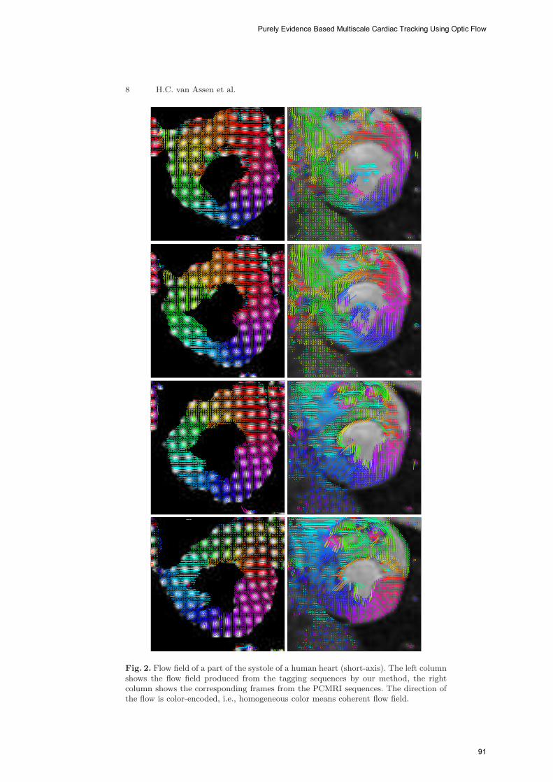
8 H.C. van Assen et al.
Fig. 2. Flow field of a part of the systole of a human heart (short-axis). The left columnshows the flow field produced from the tagging sequences by our method, the rightcolumn shows the corresponding frames from the PCMRI sequences. The direction ofthe flow is color-encoded, i.e., homogeneous color means coherent flow field.
Purely Evidence Based Multiscale Cardiac Tracking Using Optic Flow
91
Purely Evidence Based Multiscale Cardiac Tracking Using Optic Flow 9
The input “functions” f(x, y, t;σ, τ) and g(x, y, t;σ, τ) depend on the spatial andtemporal scales (σ,τ). Since the size of the tags can vary locally, a.o. due to con-traction, automatic scale selection per point was employed using the Frobeniusnorm. Also the “condition number” of the matrix C in (3) can possibly serve ascriterion for automatic scale selection. More research towards the selected scalesand the variation of chosen scales in local neighborhoods should be conducted.
References
1. Stuber, M., Scheidegger, M.B., Fischer, S.E., Nagel, E., Steinemann, F., Hess,O.M., Boesiger, P.: Alterations in the Local Myocardial Motion Pattern in PatientsSuffering From Pressure Overload Due to Aortic Stenosis. Circulation 100 (1999)361–368
2. Gunther, S., Grossman, W.: Determinants of ventricular function in pressure-overload hypertrophy in man. Circulation 59 (1979) 679–688
3. MacGowan, G.A., Shapiro, E.P., Azhari, H., Siu, C.O., Hees, P.S., Hutchins, G.M.,Weiss, J.L., Rademakers, F.E.: Noninvasive Measurement of Shortening in theFiber and Cross-Fiber Directions in the Normal Human Left Ventricle and inIdiopathic Dilated Cardiomyopathy. Circulation 96 (1997) 535–541
4. Axel, L., Dougherty, L.: MR Imaging of Motion with Spatial Modulation of Mag-netization. Radiology 171(3) (1989) 841–845
5. Fischer, S.E., McKinnon, G.C., Maier, S.E., Boesiger, P.: Improved MyocardialTagging Contrast. Magnetic Resonance in Medicine 30(2) (1993) 191–200
6. Axel, L., Chen, T., Manglik, T.: Dense Myocardium Deformation Estimationfor 2D Tagged MRI. In: Proceedings of the Third International Workshop onFunctional Imaging and Modeling of the Heart—FIMH 2005 (Barcelona, Spain,June 2005). Volume 3504 of LNCS., Berlin, Springer-Verlag (2005) 446–456
7. Pan, L., Prince, J.L., Lima, J.A.C., Osman, N.F.: Fast Tracking of Cardiac MotionUsing 3D-HARP. IEEE Transactions on Biomedical Engineering 52(8) (2005)1425–1435
8. Horn, B.K.P., Schunk, B.G.: Determining Optical Flow. Artificial Intelligence 17(1981) 185–203
9. Florack, L., Niessen, W., Nielsen, M.: The Intrinsic Structure of Optic Flow Incor-porating Measurement Duality. International Journal of Computer Vision 27(3)(1998) 263–286
10. Niessen, W.J., Duncan, J.S., ter Haar Romeny, B.M., Viergever, M.A.: Spatiotem-poral analysis of left ventricular motion. In: Medical Imaging 95, San Diego, SPIE(February 1995) 192–203
11. Niessen, W.J., Duncan, J.S., Nielsen, M., Florack, L.M.J., ter Haar Romeny, B.M.,Viergever, M.A.: A multiscale approach to image sequence analysis. ComputerVision and Image Understanding 65(2) (February 1997) 259–268
12. Suinesiaputra, A., Florack, L.M.J., Westenberg, J.J.M., ter Haar Romeny, B.M.,Reiber, J.H.C., Lelieveldt, B.P.F.: Optic flow computation from cardiac MR tag-ging using a multiscale differential method—a comparative study with velocity-encoded mri. In: Proceedings of the Sixth International Conference on MedicalImage Computing and Computer-Assisted Intervention—MICCAI 2003 (Montreal,Canada, November 2003). LNCS, Berlin, Springer-Verlag (2003) 483–490
13. Osman, N.F., Kerwin, W.S., McVeigh, E.R., Prince, J.L.: Cardiac Motion TrackingUsing CINE Harmonic Phase (HARP) Magnetic Resonance Imaging. MagneticResonance in Medicine 42(6) (1999) 1048–1060
Hans van Assen, Luc Florack, Avan Suinesiaputra, Jos Westenberg, and Bart ter Haar Romeny
92
10 H.C. van Assen et al.
14. Zerhouni, E.A., Parish, D.M., Rogers, W.J., Yang, A., Shapiro, E.P.: Human heart:tagging with MR imaging–a method for noninvasive assessment of myocardial mo-tion. Radiology 169(1) (1988) 59–63
15. Ryf, S., Tsao, J., Schwitter, J., Stuessi, A., Boesiger, P.: Peak–Combination inHARP: A Method to Correct for Phase Errors in HARP. Journal of MagneticResonance Imaging 20 (2004) 874–880
16. Sampath, S., Derbyshire, J.A., Atalar, E., Osman, N.F., Prince, J.L.: Real–Time Imaging of Two–Dimensional Cardiac Strain Using a Harmonic Phase Mag-netic Resonance Imaging (HARP–MRI) Pulse Sequence. Magnetic Resonance inMedicine 50(1) (2003) 154–163
17. Aletras, A.H., Ding, S., Balaban, R.S., Wen, H.: DENSE: Displacement Encodingwith Stimulated Echoes in Cardiac Functional MRI. Journal of Magnetic Reso-nance 137 (1999) 247–252
18. Ozturk, C., Derbyshire, J.A., McVeigh, E.R.: Estimating Motion from MRI Data.Proc. of the IEEE 91(10) (2003) 1627–1648
19. Bryant, D., Payne, J.A., Firmin, D.N., Longmore, D.B.: Measurement of flow withNMR imaging using gradient pulse and phase difference technique. Journal ofComputer Assisted Tomography 8 (1984) 588–593
20. Gotte, M.J., van Rossum, A.C., Twisk, J.W.R., et al.: Quantification of regionalcontractile function after infarction: strain analysis superior to wall thickening anal-ysis in discriminating infarct from remote myocardium. Journal of the AmericanCollege of Cardiology 37 (2001) 808–817
21. Delhaas, T., Kotte, J., van der Toorn, A., Snoep, G., Prinzen, F.W., Arts, T.:Increase in Left Ventricular Torsion-to-Shortening Ratio in Children With ValvularAorta Stenosis. Magnetic Resonance in Medicine 51 (2004) 135–139
22. Dougherty, L., Asmuth, J.C., Blom, A.S., Axel, L., Kumar, R.: Validation of anOptical Flow Method for Tag Displacement Estimation. IEEE Transactions onMedical Imaging 18(4) (1999) 359–363
23. Kraitchman, D.L., Young, A.A., Chang, C.N., Axel, L.: Semi-automatic tracking ofmyocardial motion in MR tagged images. IEEE Transactions on Medical Imaging14(3) (1995) 422–433
24. Prince, J.L., McVeigh, E.R.: Motion estimation from tagged MR image sequences.IEEE Transactions on Medical Imaging 11(2) (1992) 238–249
25. Gupta, S.N., Prince, J.L.: On Variable Brightness Optical Flow for Tagged MRI.In Bizais, Y., ed.: Information Processing in Medical Imaging: 14th InternationalConference, Ile de Berder, France, June 1995, Dordrecht, Kluwer, ISBN 0-7923-3593-7 (1995)
26. Barron, J.L., Fleet, D.J., Beauchemin, S.S.: Performance of optical flow techniques.International Journal of Computer Vision 12(1) (1994) 43–77
27. Brox, T., Bruhn, A., Papenberg, N., Weickert, J.: High accuracy optical flowestimation based on a theory for warping. In Pajdla, T., Matas, J., eds.: Proc.ECCV. Volume IV of LNCS., Berlin, Springer-Verlag (May 2004) 25–36
28. Bruhn, A., Weickert, J., Feddern, C., Kohlberger, T., Schnorr, C.: Relations be-tween regularization and diffusion filtering. IEEE Transactions on Image Process-ing 14(5) (2005) 608–615
29. Weickert, J., Schnorr, C.: Variational optic flow computation with a spatio-temporal smoothness constraint. Journal of Mathematical Imaging and Vision14(3) (2001) 245–255
30. Kuijer, J.P.A., Jansen, E., Marcus, J.T., van Rossum, A.C., Heethaar, R.M.: Im-proved harmonic phase myocardial strain maps. Magnetic Resonance in Medicine46(5) (2001) 993–999
Purely Evidence Based Multiscale Cardiac Tracking Using Optic Flow
93

3-D Non-Linear Finite Element Analysis of Normal Pressure Hydrocephalus
Tonmoy Dutta-Roy, Adam Wittek, Karol Miller
Intelligent Systems for Medicine Laboratory, School of Mechanical Engineering, M050, University of Western Australia, 35 Stirling Highway, Crawley, WA, Australia 6009
{tduttar, kmiller, adwit}@mech.uwa.edu.au
Abstract. This paper presents the mechanics of Normal Pressure Hydrocephalus (NPH) growth using a computational approach. We generated a generic 3-D mesh of a healthy human brain and treated the brain parenchyma as single and biphasic continuum with non-linear constitutive law undergoing finite deformations. Contact boundary conditions constrained the brain which is enclosed in a skull. We loaded the brain using transmantle pressure difference. Non-linear, implicit, Finite-Element (FE) procedures in time domain were used to obtain the deformations for the brain and ventricles. We propose that for modelling NPH, there is no significant advantage gained by using biphasic continuum to model brain parenchyma and that single phase continuum is adequate. We obtained almost equal ventricular volume for both single and biphasic treatment of brain parenchyma under same loading condition. The use of single phase continuum simplified the mathematical description for the model and resulted in large saving of computational time.
1 Introduction
Overlap of symptoms and diagnostic findings between Normal Pressure Hydrocephalus (NPH) and other neurodegenerative diseases (Alzheimer’s etc) makes diagnosis of NPH a reoccurring problem for clinicians. Hakim and Adams [1] were the first to identify the condition of NPH. Currently, clinical and diagnostic findings of neurosurgeons in combination with engineering principles enhance the diagnosis of NPH [2, 3, 4 and 5], but these approaches offer no insight into NPH growth mechanics.
Hakim [6] proposed a “sponge” type model of brain parenchyma for NPH growth but without any mathematical formulations. Nagashima et al. [7] and Péna et al. [8] utilised coupled pore fluid diffusion and stress analysis (biphasic approach) for a linear elastic model of brain parenchyma (porous medium) undergoing infinitesimal deformations on a 2-D horizontal brain slice obtained from a brain atlas. Kaczmarek et al [9] used finite deformation biphasic theory on simplified brain geometry (cylindrical) and obtained an analytical solution. Taylor and Miller [10] utilised reassessed brain parenchyma elastic modulus and finite deformation biphasic theory on realistic 2-D brain geometry. Apart from NPH analysis, Miga et al. [11], Miga et al. [12], Paulsen et al. [13], Platenik et al. [14] and Lunn et al. [15] used biphasic
94
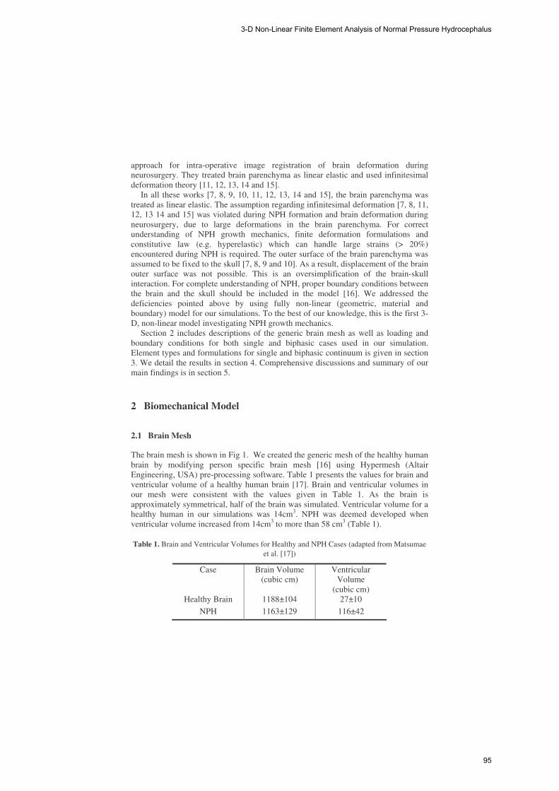
approach for intra-operative image registration of brain deformation during neurosurgery. They treated brain parenchyma as linear elastic and used infinitesimal deformation theory [11, 12, 13, 14 and 15].
In all these works [7, 8, 9, 10, 11, 12, 13, 14 and 15], the brain parenchyma was treated as linear elastic. The assumption regarding infinitesimal deformation [7, 8, 11, 12, 13 14 and 15] was violated during NPH formation and brain deformation during neurosurgery, due to large deformations in the brain parenchyma. For correct understanding of NPH growth mechanics, finite deformation formulations and constitutive law (e.g. hyperelastic) which can handle large strains (> 20%) encountered during NPH is required. The outer surface of the brain parenchyma was assumed to be fixed to the skull [7, 8, 9 and 10]. As a result, displacement of the brain outer surface was not possible. This is an oversimplification of the brain-skull interaction. For complete understanding of NPH, proper boundary conditions between the brain and the skull should be included in the model [16]. We addressed the deficiencies pointed above by using fully non-linear (geometric, material and boundary) model for our simulations. To the best of our knowledge, this is the first 3-D, non-linear model investigating NPH growth mechanics.
Section 2 includes descriptions of the generic brain mesh as well as loading and boundary conditions for both single and biphasic cases used in our simulation. Element types and formulations for single and biphasic continuum is given in section 3. We detail the results in section 4. Comprehensive discussions and summary of our main findings is in section 5.
2 Biomechanical Model
2.1 Brain Mesh
The brain mesh is shown in Fig 1. We created the generic mesh of the healthy human brain by modifying person specific brain mesh [16] using Hypermesh (Altair Engineering, USA) pre-processing software. Table 1 presents the values for brain and ventricular volume of a healthy human brain [17]. Brain and ventricular volumes in our mesh were consistent with the values given in Table 1. As the brain is approximately symmetrical, half of the brain was simulated. Ventricular volume for a healthy human in our simulations was 14cm3. NPH was deemed developed when ventricular volume increased from 14cm3 to more than 58 cm3 (Table 1).
Table 1. Brain and Ventricular Volumes for Healthy and NPH Cases (adapted from Matsumae et al. [17])
Case Brain Volume (cubic cm)
Ventricular Volume
(cubic cm) Healthy Brain 1188±104 27±10
NPH 1163±129 116±42
3-D Non-Linear Finite Element Analysis of Normal Pressure Hydrocephalus
95

2.1.1 Modified Hyperelastic Material Parameters The stress-strain behaviour of the brain parenchyma is non-linear with stiffness in compression significantly higher than tension with strong stress-strain rate dependency [18, 19]. To account for these complexities in the brain parenchyma, we chose the hyper-viscoelastic constitutive model proposed by Miller and Chinzei [19].
The time required for NPH growth is relatively long (typically 4 days) [7] when compared to surgical interventions and loading of the brain occurs very slowly. Thus, the strain rate dependency of the brain parenchyma disappeared [10]. Hence, the brain parenchyma was modelled as hyperelastic (Ogden form [20]) given by:
)3(2
W 3212−λ+λ+λ
α
μ= ααα (1)
where, W is the potential function, �i’s are the principal stretches, � is the relaxed shear modulus and � is the material coefficient which can assume any real value without any restrictions. The value � was 155.77 Pa [10] and the value of � was -4.7 [10]. We considered the brain parenchyma to be homogenous and isotropic for simulation purposes [21] as the brain tissue does not exhibit directional structure, unless the behaviour of very small tissue specimens is of interest [22].
Fig. 1. Brain geometry, pressure loading and applied boundary conditions
2.1.1.1 Biphasic Continuum Brain was considered to be a sponge like structure with the solid matrix corresponding to neurons and neuroglia and voids being extracellular space [1, 6] occupied by CSF. This is referred to as biphasic [7, 8, 9, 10, 11, 12, 13, 14, 15 and 22] continuum because of presence of two phases: brain parenchyma (solid or porous phase) and CSF (fluid phase). To understand the interaction between brain parenchyma and CSF when loaded by a given transmantle pressure difference, we performed a coupled pore fluid diffusion and stress analysis. The reader may refer to
Skull Plane 1
Bottom nodes constrained
Brain Parenchyma
Transmantle Pressure Difference
Ptrans
Ventricles
Tonmoy Dutta-Roy, Adam Wittek, Karol Miller
96

the works of Nagashima et al. [7], Miller [23], Biot [24], and Bowen [25] for detailed discussions on the mathematical treatment of biphasic continuum.
In our model, brain parenchyma (solid phase) had a Poisson’s ratio (�) of 0.35 [7, 8, 9, 10, and 22] with relaxed hyperelastic material properties (section 2.1.1), initial void ratio of 0.2 [7, 26] and permeability of 1.59x10⁻⁷ m/sec [9]. It was fully saturated with CSF. CSF (fluid phase) was incompressible, non-viscous with mechanical properties of water.
2.1.1.2 Single Phase Continuum Due to long development time for NPH, there existed possibility of Cerebrospinal Fluid (CSF) to be absorbed or evacuated in the brain parenchyma, resulting in CSF flow within it and change in brain and ventricular volume. We treated the brain parenchyma as compressible single phase continuum with non-linear constitutive law [19] (generalisation of Ogden rubber [23]), relaxed hyperelastic shear modulus (section 2.1.1) and a low Poisson’s ratio of 0.35 [7, 8, 9, 10, and 22] and investigated this effect of compressibility.
2.2 Loading Load was a transmantle pressure difference (Ptrans) in form of pressure on the ventricular surfaces as shown in Fig 1. There was no pressure acting on the outer surface of the brain. It is a widely held view that transmantle pressure difference (Ptrans) of 1mm of Hg (133.416 Pa) produced the clinical condition of NPH [27, 28] and the same was applied to the ventricular surface to investigate this claim.
2.2.1 Biphasic Continuum Even though material strain rate effects were absent due to use of hyperelastic constitutive law for the brain parenchyma, rate effects were present because of relative motion between brain parenchyma (solid phase) and CSF (fluid phase). The time period of load application was of importance and transmantle pressure difference (Ptrans) was applied over the development time of NPH (4 days) using a polynomial which provided zero velocity and acceleration respectively at the beginning and end of the loading.
2.2.2 Single Phase Continuum The time period of load application was not important as we seek a static solution for the single phase continuum and material strain rate effects were absent due to use of hyperelastic constitutive law for the brain parenchyma. Hence, time period of transmantle pressure difference (Ptrans) application was arbitrarily taken to be 10 seconds.
2.3 Boundary Conditions As the brain is approximately symmetrical about the mid-sagittal axis, half of the brain for both single and biphasic continuum was simulated. The nodes on plane 1 (Fig 1) had symmetrical boundary conditions in YZ plane (no motion allowed for X translation) applied to them. As the brain was resting in the skull, we constrained the
3-D Non-Linear Finite Element Analysis of Normal Pressure Hydrocephalus
97

brain bottom nodes in Y and Z translation (Fig 1). A skull enclosed the brain and frictionless, finite sliding; node-to-surface penalty contact between the brain and skull constrained the nodes on the brain outer surface. Following Wittek et al. [16], Sub-Arachnoid’s Space (SAS) was accounted by a 3mm gap between the skull and the brain outer surface.
2.3.1 Biphasic Continuum There exists a pressure gradient between the ventricles and Sub-Arachnoid’s Space (SAS) resulting in flow of CSF from ventricles to SAS. We set the pore pressure on the ventricular surface equal to the transmantle pressure difference (Ptrans) and 0 Pa on the outer surface of the brain and implemented this pressure gradient.
3 Computational Model
3.1 Brain Mesh
3.1.1 Biphasic Continuum 5858 porohyperelastic type C3D20PH (20 node triquadratic displacement, trilinear pore pressure, mixed formulation with linear pressure, pore pressure) [29] and 89 type C3D10H (10 node quadratic tetrahedron, mixed formulation with linear pressure, stress displacement) [29] elements discretised the brain parenchyma. We used mixed formulation quadratic tetrahedrons to complete the brick dominated mesh. Volumetric locking was not shown by both C3D20PH and C3D10H type elements.
3.1.2 Single Phase Continuum The brain parenchyma consisted of 5858 type C3D20H (20 node quadratic brick, mixed formulation with linear pressure, stress displacement) [29] and 89 type C3D10H (10 node quadratic tetrahedron, mixed formulation with linear pressure, stress displacement) [29] elements. As mentioned earlier, we used mixed formulation quadratic tetrahedrons to complete the brick dominated mesh. Type C3D20H did not exhibit volumetric locking for incompressible/nearly incompressible continuum (e.g. brain).
3.2 Skull The skull consisted of 1006 type R3D4 (4 node, bilinear quadrilateral, 3-D rigid) [29] elements.
3.3 Finite Element Solver We obtained the solution for NPH growth model using ABAQUS/Standard (Abaqus Inc, Providence, Rhode Island, USA) non-linear finite element code (ABAQUS/Standard, 2004) [32]. The code accounted for geometric, constitutive and contact non-linearities. STATIC (fully non-linear, finite deformation) procedure obtained solution for single phase continuum case and SOILS (fully non-linear, finite
Tonmoy Dutta-Roy, Adam Wittek, Karol Miller
98
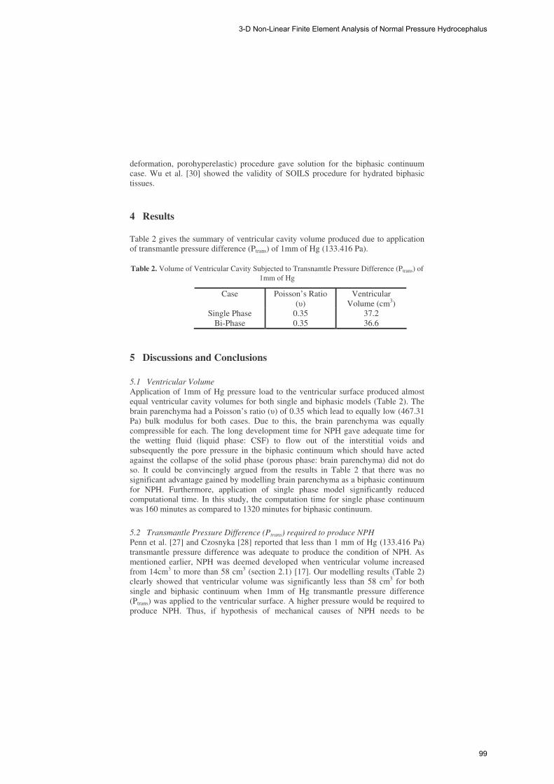
deformation, porohyperelastic) procedure gave solution for the biphasic continuum case. Wu et al. [30] showed the validity of SOILS procedure for hydrated biphasic tissues.
4 Results
Table 2 gives the summary of ventricular cavity volume produced due to application of transmantle pressure difference (Ptrans) of 1mm of Hg (133.416 Pa).
Table 2. Volume of Ventricular Cavity Subjected to Transnamtle Pressure Difference (Ptrans) of 1mm of Hg
Case Poisson’s Ratio (�)
Ventricular Volume (cm3)
Single Phase 0.35 37.2 Bi-Phase 0.35 36.6
5 Discussions and Conclusions
5.1 Ventricular Volume Application of 1mm of Hg pressure load to the ventricular surface produced almost equal ventricular cavity volumes for both single and biphasic models (Table 2). The brain parenchyma had a Poisson’s ratio (�) of 0.35 which lead to equally low (467.31 Pa) bulk modulus for both cases. Due to this, the brain parenchyma was equally compressible for each. The long development time for NPH gave adequate time for the wetting fluid (liquid phase: CSF) to flow out of the interstitial voids and subsequently the pore pressure in the biphasic continuum which should have acted against the collapse of the solid phase (porous phase: brain parenchyma) did not do so. It could be convincingly argued from the results in Table 2 that there was no significant advantage gained by modelling brain parenchyma as a biphasic continuum for NPH. Furthermore, application of single phase model significantly reduced computational time. In this study, the computation time for single phase continuum was 160 minutes as compared to 1320 minutes for biphasic continuum.
5.2 Transmantle Pressure Difference (Ptrans) required to produce NPH Penn et al. [27] and Czosnyka [28] reported that less than 1 mm of Hg (133.416 Pa) transmantle pressure difference was adequate to produce the condition of NPH. As mentioned earlier, NPH was deemed developed when ventricular volume increased from 14cm3 to more than 58 cm3 (section 2.1) [17]. Our modelling results (Table 2) clearly showed that ventricular volume was significantly less than 58 cm3 for both single and biphasic continuum when 1mm of Hg transmantle pressure difference (Ptrans) was applied to the ventricular surface. A higher pressure would be required to produce NPH. Thus, if hypothesis of mechanical causes of NPH needs to be
3-D Non-Linear Finite Element Analysis of Normal Pressure Hydrocephalus
99
sustained, measurement of transmantle pressure difference (Ptrans) required to produce NPH should be reassessed.
5.4 Conclusions
Our work showed that application of 1mm of Hg transmantle pressure difference (Ptrans) resulted in almost equal ventricular volume for both single and biphasic models. Hence, we recommend use of single phase continuum model for brain parenchyma. The use of single phase continuum simplified the mathematical description of the system and lead to shorter computational time. According to our modelling results, 1 mm of Hg transmantle pressure difference (Ptrans) as reported by other authors was not adequate to produce NPH for both single and biphasic models This suggested that measurement of transmantle pressure difference (Ptrans) required for producing NPH needed reassessment, if hypothesis of mechanical causes of NPH was to be sustained.
Acknowledgements Financial support of the William and Marlene Schrader Trust in form of William and Marlene Schrader Post-Graduate Scholarship for the first author is gratefully acknowledged.
References
1. Hakim, S. and Adams, R.D.: The Special Clinical Problem of Symptomatic Hydrocephalus with Normal Cerebrospinal Fluid Pressure: Observations on Cerebrospinal Fluid Hydrodynamics, Journal of the Neurological Sciences. 2 (1965), 307-327.
2. Linninger, A. A., Tsakiris, C., Zhu, D. C., Xenos, M., Roycewicz, P., Danziger, Z. and Penn, R.: Pulsatile Cerebrospinal Fluid Dynamics in the Human Brain, IEEE Transactions on Biomedical Engineering 52 (2005 557-565.
3. Shulman, K. and Marmarou, A.: Analysis of Intracranial Pressure in Hydrocephalus, Developmental Medicine and Child Neurology Suppl 16 (1968), 11-16.
4. Marmarou, A., Shulman, K. and Rosende, R.M.: A Non-linear Analysis of CSF System and Intracranial Pressure Dynamics, Journal of Neurosurgery 48 (1978), 332-344.
5. Czosnyka, M., and Pickard, J.D.: Monitoring and Interpretation of Intracranial Pressure, Journal of Neurology, Neurosurgery and Psychiatry 75 (2004), 813-821.
6. Hakim S.: Biomechanics of Hydrocephalus, Acta Neurológica Latinoamericana 1 Suppl 1 (1971), 169-194.
7. Nagashima, T., Tamaki, N., Matsumoto, S., Horwitz, B. and Seguchi, Y.: Biomechanics of Hydrocephalus: A New Theoretical Model, Neurosurgery 21 (1987), 898-904.
8 Pena, A., Bolton, M.D., Whitehouse, H. and Pickard, J.D.: Effects of Brain Ventricular Shape on Periventricular Biomechanics: A Finite Element Analysis, Neurosurgery 45 (1999), 107-118.
9. Kaczmarek, M., Subramaniam, R.P. and Neff, S.R.: The Hydromechanics of Hydrocephalus: Steady-State Solutions for Cylindrical Geometry, Bulletin of Mathematical Biology 59 (1997), 295-323.
Tonmoy Dutta-Roy, Adam Wittek, Karol Miller
100

10. Taylor, Z. and Miller, K.: Reassessment of Brain Elasticity for Analysis of Biomechanisms of Hydrocephalus, Journal of Biomechanics 37 (2004), 1263-1269.
11 Miga, M. I., Paulsen, K. D., Lemery, J. M., Eisner, S. D., Hartov, A., Kennedy, F. E. and Roberts, D. W.: Model-Updated Image Guidance: Initial Clinical Experiences with Gravity-Induced Brain Deformation. IEEE Transactions on Biomedical Engineering, 18 (1999), 866-874.
12. Miga, M.I., Paulsen, K.D., Hoopes, P.J., Kennedy, F.E. Jnr, Hartov, A., and Roberts, D.W.: In-vivo Quantification of a Homogeneous Brain Deformation Model for Updating Preoperative Image Guiding Surgery, IEEE Transactions on Biomedical Engineering 47 (2000), 266-273.
13. Paulsen, K. D., Miga, M. I., Kennedy, F. E., Hoops, P. J., Hartov, A. and Roberts, D. W.: A Computational Model for Tracking Subsurface Tissue Deformation during Stereotactic Neurosurgery, IEEE Transactions on Biomedical Engineering, 46 (1999), 213-225.
14 Platenik, L. A., Miga, M. I., Roberts, D. W., Lunn, K. E., Kennedy, F. E., Hartov, A. and Paulsen, K. D.: In Vivo Quantification of Retraction Deformation Modelling for Updated Image-Guidance during Neurosurgery. IEEE Transactions on Biomedical Engineering, 49 (2002), 823-835.
15. Lunn, K. E., Paulsen, K.D., Liu, F., Kennedy, F.E., Hartov, A. and Roberts, D.W.: Data-Guided Brain Deformation Modelling: Evaluation of a 3-D Adjoint Inversion Method in Porcine Studies. IEEE Transactions on Bio-Medical Engineering, 53 (2006), 1893-1900.
16. Wittek, A., Karol, M., Kikinis, R. and Warfield, S.K.: Patient-Specific Model of Brain Deformation: Application to Medical Image Registration, Journal of Biomechanics 40 (2007), 919-929.
17. Matsumae, M., Kikinis, R., Morocz, I., Lorenzo, A.V., Albert, M.S., Black, P. McL., and Jolesz, F.A.: Intracranial Compartment Volumes in Patients with Enlarged Ventricles Assessed by Magnetic Resonance-Based Image Processing, Journal of Neurosurgery 84 (1996), 972-981.
18. Miller K. and Chinzei K.: Constitutive Modelling of Brain Tissue: Experiment and Theory, Journal of Biomechanics 30 (1997), 1115-1121.
19. Miller, K. and Chinzei, K.: Mechanical Properties of Brain Tissue in Tension, Journal of Biomechanics 35 (2002), 483-490.
20. Ogden, R.W.: Non-Linear Elastic Deformations, Ellis Horwood Ltd., Chichester, Great Britain, (1984).
21. Ozawa, H., Matsumoto, S., Ohashi, T., Sato, M. and Kokubun, S.: Comparison of Spinal Cord Gray and White Matter Softness: Measurement of Pipette Aspiration Method, Journal of Neurosurgery 95 (2001), 221-224.
22. Miller, K., Taylor, Z. and Nowinski, W.L.: Towards Computing Brain Deformation for Diagnosis, Prognosis and Neurosurgical Simulations, Journal of Mechanics in Medicine and Biology 5 (2005), 105-121.
23. Miller, K.: Modelling Soft Tissues Using Biphasic Theory-A Word of Caution, Computer Methods in Biomechanics and Biomedical Engineering 1 (1998), 216-263.
24. Biot, M.A.: General Theory of Three-Dimensional Consolidation, Journal of Applied Physics 12 (1941), 1244-1258.
25. Bowen, R.M.: Theory of Mixtures, vol. III, Academic Press, New York, (1976). 26. Sykova, E: Diffusion Properties of the Brain in Health and Disease, Neurochemistry
International 45 (2004), 453-466. 27. Penn, R.D., Max, C.L., Linninger, A. A., Miesel, K., Lu, S.N. and Stylos, L.: Pressure
Gradients in the Brain in an Experimental Model of Hydrocephalus, Journal of Neurosurgery 102 (2005), 1069-1075.
28. Czosnyka, M.: Telephonic Conversation, (2006). 29. ABAQUS: ABAQUS/Standard Manual, Version 6.5.4, Hibbit, Karlsson and Sorenson, Inc.
(2004).
3-D Non-Linear Finite Element Analysis of Normal Pressure Hydrocephalus
101

30. Wu, J.Z., Herzog, W. and Epstein, M.: Evaluation of the Finite Element Software ABAQUS for Biomechanical Modeling of Biphasic Tissues, Journal of Biomechanics 31 (1998), 165-169.
Tonmoy Dutta-Roy, Adam Wittek, Karol Miller
102

Computational Biomechanics of the Breast: TheImportance of the Reference State
Vijay Rajagopal1, Angela Lee1 Jae-Hoon Chung1, Poul M.F. Nielsen1, andMartyn P. Nash1
Bioengineering Institute, University of Auckland, NZ, [email protected]
Abstract. Breast cancer diagnosis involves the analysis and interpreta-tion of images of the breast acquired using a variety of imaging modalitiessuch as ultrasound, x-ray mammography and magnetic resonance (MR).Biomechanical models of the breast could help track tissue movementand thereby assist in the interpretation of image patterns across multi-ple imaging modalities. To this end, we are developing a software systemfor the creation of subject-specific finite element models of the breast thatis systematically validated and optimised for use in the clinical setting.
In this paper, we describe a pilot study conducted in order to determinethe sensitivity of deformation predictions to the accuracy of the repre-sentation of the reference state - an issue that has been overlooked inprevious studies. Predictions of the supine gravity-loaded configurationof the breast of a volunteer from (i) a model that uses the prone gravity-loaded state as the reference state (without applying initial stresses toaccount for gravity), and (ii) a model that uses the breast configurationin neutral buoyancy (immersed in water, assuming the density of thebreast is close to that of water) were compared.
The model using the prone gravity-loaded state as the reference configu-ration predicted the supine gravity-loaded anterior surface configurationwith an RMS error of 11.4 mm, while the model using the neutral buoy-ancy state as the reference configuration predicted the supine configura-tion with an RMS error of 6.7 mm. These results indicate the selection ofa reference state of the breast is an important aspect in the developmentof a reliable biomechanical model of the breast.
1 Introduction
Diagnostic procedures for breast cancer require interpretation of image patternsby experienced clinicians. Recent studies have highlighted the importance ofexperience and the examination of the breast using a variety of view-points forintra-modality (x-ray cranio-caudal and medio-lateral, for example) as well asinter-modality (x-ray, MRI, ultrasound) imaging [1, 2]. When imaging the breastusing these different modalities, it undergoes significant changes in shape, andthe displacements of the internal tissues are governed by the laws of physics.
Image registration techniques have been developed to account for these dis-placements so that a clinician may more easily track and assess a specific region
103
of tissue across different views. However, a number of these registration tech-niques have traditionally based their computations on image-intensity statisticssuch as mutual information and center of mass [3–5]. These techniques providetransformations between images that are typically heuristic and can prove to beunreliable.
For instance, Tanner et al [6] showed that the method proposed in [3] could beimproved by introducing a volume-preserving constraint. The need for volume-preserving constraints indicated that non-rigid registration algorithms requirefurther validation to measure the accuracy of the transformations in captur-ing the tissue deformations during imaging. An important aspect of these tech-niques that had not been addressed until recently, is the physical-plausibility ofthe transformations from these heuristic methods. Finite element models of thebreast are now being developed to provide physics-based constraints to imageregistration algorithms [7–11]. Anatomically realistic biomechanical models ofthe breast can potentially assist clinicians in diagnosing breast cancer by pro-viding them with an image visualisation and patient data management system.
Due to the non-linear nature of large deformations that breast tissue undergoduring imaging procedures, large errors in the representation of a reference statewill lead to large errors in model predictions. While the senstivity of model pre-dictions to the choice of boundary conditions and material parameters have beenaddressed [9, 12], most studies have overlooked the importance of correctly rep-resenting the reference state of the breast either: as stress-free in an unloadedconfiguration; or as initially stressed in a known loaded configuration by pro-viding the three-dimensional stress distribution. Researchers have typically useda gravity-loaded configuration of the breast (such as the prone or supine con-figuration) without providing information on the three-dimensional stresses inthe chosen state [10, 11]. To the authors’ knowledge, this is the first study thatinvestigates the use of the unloaded state as the reference configuration and thesensitivity of model predictions to errors in the representation of the referencestate.
We first describe the methods used to create finite element models of thebreast. We then compare the predictions of a particular gravity-loaded configu-ration of the breast of a volunteer from: (i) a biomechanical model that uses theprone gravity-loaded configuration as the reference state (with no initial stressesapplied to account for gravity); and (ii) a biomechanical model that uses thebreast configuration in neutral buoyancy (immersed in water, thus removing theeffects of gravity loading) as the reference configuration.
2 Methods
We use our in-house modelling software, CMISS [13], to predict breast deforma-tions. We use the finite element implementation of finite deformation elasticitytheory to model breast biomechanics. The reader is referred to standard textssuch as [14] and [15] for detailed descriptions of finite elasticity theory and the
Vijay Rajagopal, Angela Lee Jae-Hoon Chung, Poul M.F. Nielsen, and Martyn P. Nash
104

finite element method. The following sections briefly describe the methods weuse to generate and use subject-specific models of the breast.
2.1 Subject-specific breast geometry
We create subject-specific breast geometries by fitting faces of hexahedral, cubic-Hermite elements to skin and muscle surface data sets that have been segmentedfrom MR images (see Fig. 1). The surfaces are fitted using a least squares ap-proach, as described in [16]. The customisation process has been optimised torun in an automatic fashion (with minimal user intervention) in order to gener-ate breast models rapidly as would be required in a clinical setting. The readeris directed to [7] and [17] for further details on the customisation process and itsperformance with different breast shapes. We found that geometric finite elementmodels consisting of 24 tri-cubic Hermite elements (with 70 nodes and 1680 totalgeometric degrees of freedom) fitted the models with an average overall RMSerror of 1.5 mm in representing the skin and muscle surfaces. For the mechanicsstudy presented here, the breast was assumed to be homogeneous after [8], thusthe geometrical model did not need to account for any structural differencesbetween the internal tissues.
(a) (b) (c) (d)
Fig. 1. Process of creating a subject-specific breast model. (a): Segmentation of tissueboundaries. Green points represent the skin surface, and red points represent musclesurface. (b): Dataset of skin (brown points), and muscle (red points) after segmentingan entire MR image set. (c): Initial finite element model whose external faces are tobe fitted to the skin and muscle data sets. (d): Finite element model fitted to skin andmuscle surfaces.
2.2 Loading and boundary Conditions
Gravity loading was applied as a body force to the reference state of the model(see Section 2.4 regarding the reference configuration). No initial stresses were
Computational Biomechanics of the Breast: The Importance of the Reference State
105
applied to the prone gravity-loaded reference configuration to account for grav-ity. For the purposes of this study, it was assumed that the breast tissues andmuscle were firmly attached to the rib cage, thus we applied fixed-displacementboundary conditions at the posterior surface of the model. Previous models haveapplied displacement boundary conditions to nodes across the entire skin surfaceto ensure that they matched the outer shape of the breast in the deformed con-figuration [9, 8, 10]. In contrast, the simulations in the present study are drivenby the gravity loading condition alone and thus provide a more robust way ofassessing the ability of the model to predict breast deformations.
2.3 Subject-specific constitutive parameters
The breast was assumed to be incompressible, homogeneous and isotropic af-ter [8]. A number of experimental studies have been conducted to characterisethe mechanical behaviour of breast tissues [18, 19]. Previous researchers havetypically used the experimental data from the literature to fit the material con-stant, c1, in the neo-Hookean constitutive equation W = c1(I1 − 3), where I1is the first principal invariant of the Lagrangian strain tensor [14]. However, itis well known from experiments that breast tissue mechanical properties varysignicantly between subjects [20]. Therefore, it is likely to be important to fitthe material constant to each individual. We used our existing material param-eter optimisation techniques [21] to estimate the value of c1 using the modelof the reference shape together with segmented data from images of differentgravity-loaded configurations.
2.4 The reference configuration and its importance
In this paper, we investigate the importance of the selection of a reference state ofthe breast. We conducted this study by comparing the performances of a modelin predicting gravity-loaded configurations when two different representations ofthe reference state of the breast were used.
The breast of a volunteer was imaged in four different configurations (see Fig.2): (i) prone gravity-loaded (ii) supine gravity-loaded (iii) 11.5 degrees “head up”(the volunteer is in a prone position with their back arched slightly upwards, suchthat the head is raised.) (iv) prone and neutrally buoyant by assuming that thedensity of the breast is close to that of water and submerging the breast inwater. For this last case, we assume that neutral buoyancy offsets the effects ofgravity, and more closely represents the stress-free reference configuration of thebreast. These images are the first to capture the unloaded shape of the breastand allow us to quantify the importance of the representation of the referenceconfiguration on the accuracy of breast mechanics modelling using clinical data.
Vijay Rajagopal, Angela Lee Jae-Hoon Chung, Poul M.F. Nielsen, and Martyn P. Nash
106

(a)
(b)
(c)
(d)
Fig. 2. MR images of the breast in four different orientations: (a): prone gravity-loadedconfiguration. (b): supine gravity-loaded configuration. (c): 11.5 degrees head up, wherethe volunteer is in a prone position with their back arched slightly upwards, suchthat the head is raised. (d): prone and neutrally buoyant configuration, obtained byassuming that the density of the breast is close to that of water and submerging thebreast in water. Only the right breast was immersed in water in this study.
Computational Biomechanics of the Breast: The Importance of the Reference State
107
With these image sets, two different sets of simulations were conducted andare described as follows:
– Using the neutral buoyant configuration as the reference state: Theneutral buoyancy configuration was assumed to represent the reference stateof the breast and a model of this configuration was created using the cus-tomisation process described in Section 2.1. The model was then subjectedto the “head up” gravity loading condition, and the value of c1 in the neo-Hookean constitutive equation was estimated using non-linear optimisation,with the objective of minimising the error in predicting breast deformationin the “head up” orientation. The accuracy of the model prediction wasquantified by comparing the manually segmented head up configuration ofthe breast skin to the model predicted anterior surface configuration. Thesegmented points were projected (using a closest orthogonal projection ap-proach [16]) onto the deformed surface of the model, and an RMS error ofthe data projection vectors was calculated as a performance measure. Thesupine configuration of the breast was then predicted using the optimal ma-terial parameter value and compared to the skin data set that was segmentedfrom the supine configuration MR images.
– Using the prone gravity-loaded configuration as the reference state:The same procedures for material parameter optimisation and supine config-uration prediction were done as previously, but this time the prone gravity-loaded configuration (with no initial stresses due to gravity applied) wasassumed to represent the reference state of the breast.
3 Results
3.1 The neutral buoyancy configuration
The geometric finite element model of the neutrally buoyant breast had an RMSerror of 0.78 mm for fitting the skin surface and 1.2 mm for fitting the musclesurface of the volunteer’s breast.
Prior to characterising the mechanical properties of the breast, a displace-ment solution mesh convergence analysis was performed for the mechanics modelby tracking material points in the model and recording their displacements forsuccessive mesh refinements during the convergence analysis. The Euclidean dis-placements that each material point underwent during the deformation was cal-culated for each mesh resolution. The RMS errors between successive refine-ments were then recorded and the mesh corresponding to 112 tri-cubic Hermiteelements, as illustrated in Fig. 3 (216 nodes; 5184 geometric degrees of freedom),was chosen as the most appropriate resolution for reliable model predictions.
This mesh was then used to characterise the mechanical behaviour of thebreast using the “head up” configuration and the material parameter optimisa-tion technique estimated a value of c1 = 0.08 kPa for this model, which predictedthe “head up” configuration with an RMS error of 5.4 mm. The supine config-uration was then predicted using this subject-specific model and had an RMS
Vijay Rajagopal, Angela Lee Jae-Hoon Chung, Poul M.F. Nielsen, and Martyn P. Nash
108

0
0.5
1
1.5
2
2.5
5184 3240 2520
RM
S e
rror
in E
uclid
ian
disp
lace
men
t
Mesh degrees of freedom
Fig. 3. Top: Convergence of RMS error in Euclidean displacements of selected mate-rial points inside the fitted neutral buoyancy model with increasing mesh resolution.Bottom: Chosen resolution for mechanics model predictions.
error of 6.7 mm in capturing the experimentally observed breast deformation(see Fig. 4).
3.2 The prone gravity-loaded configuration
The geometric finite element model of the prone gravity-loaded breast had anRMS error of 0.6 mm for fitting the skin surface and 1.0 mm for fitting the musclesurface of the volunteer’s breast. The mesh was refined in the same manner as inthe neutral buoyancy simulation study to ensure reliable displacement convergedmodel predictions. This mesh was then used to characterise the mechanical be-haviour of the breast using the “head up” configuration. The material parameteroptimisation technique estimated a value of c1 = 50 kPa for this model, whichpredicted the “head up” configuration with an RMS error of 4.0 mm. The supineconfiguration was then predicted using this subject-specific model and had anRMS error of 11.4 mm in capturing the experimentally observed breast defor-mation (see Fig. 5).
Computational Biomechanics of the Breast: The Importance of the Reference State
109
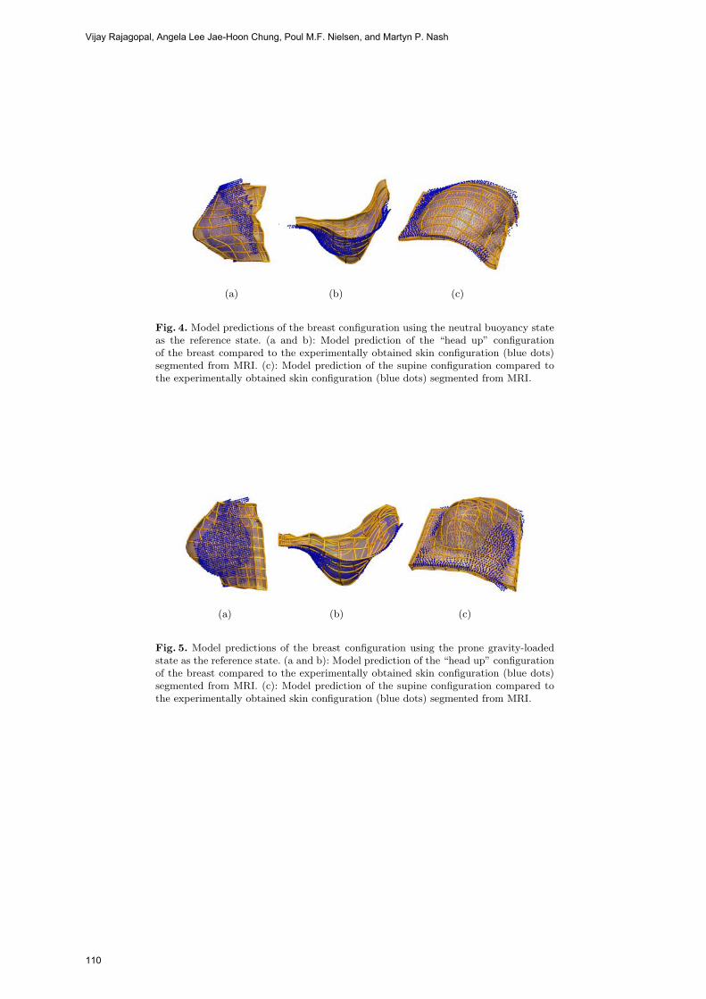
(a) (b) (c)
Fig. 4. Model predictions of the breast configuration using the neutral buoyancy stateas the reference state. (a and b): Model prediction of the “head up” configurationof the breast compared to the experimentally obtained skin configuration (blue dots)segmented from MRI. (c): Model prediction of the supine configuration compared tothe experimentally obtained skin configuration (blue dots) segmented from MRI.
(a) (b) (c)
Fig. 5. Model predictions of the breast configuration using the prone gravity-loadedstate as the reference state. (a and b): Model prediction of the “head up” configurationof the breast compared to the experimentally obtained skin configuration (blue dots)segmented from MRI. (c): Model prediction of the supine configuration compared tothe experimentally obtained skin configuration (blue dots) segmented from MRI.
Vijay Rajagopal, Angela Lee Jae-Hoon Chung, Poul M.F. Nielsen, and Martyn P. Nash
110
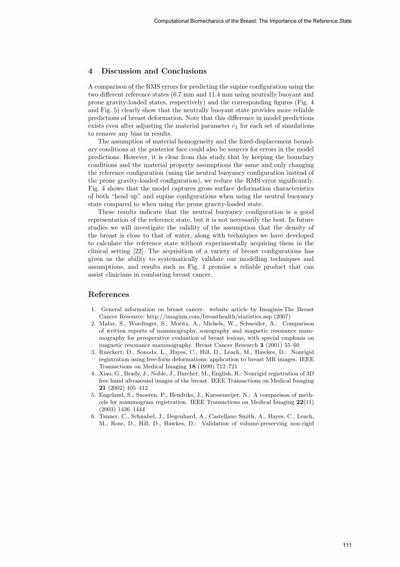
4 Discussion and Conclusions
A comparison of the RMS errors for predicting the supine configuration using thetwo different reference states (6.7 mm and 11.4 mm using neutrally buoyant andprone gravity-loaded states, respectively) and the corresponding figures (Fig. 4and Fig. 5) clearly show that the neutrally buoyant state provides more reliablepredictions of breast deformation. Note that this difference in model predictionsexists even after adjusting the material parameter c1 for each set of simulationsto remove any bias in results.
The assumption of material homogeneity and the fixed-displacement bound-ary conditions at the posterior face could also be sources for errors in the modelpredictions. However, it is clear from this study that by keeping the boundaryconditions and the material property assumptions the same and only changingthe reference configuration (using the neutral buoyancy configuration instead ofthe prone gravity-loaded configuration), we reduce the RMS error significantly.Fig. 4 shows that the model captures gross surface deformation characteristicsof both “head up” and supine configurations when using the neutral buoyancystate compared to when using the prone gravity-loaded state.
These results indicate that the neutral buoyancy configuration is a goodrepresentation of the reference state, but it is not necessarily the best. In futurestudies we will investigate the validity of the assumption that the density ofthe breast is close to that of water, along with techniques we have developedto calculate the reference state without experimentally acquiring them in theclinical setting [22]. The acquisition of a variety of breast configurations hasgiven us the ability to systematically validate our modelling techniques andassumptions, and results such as Fig. 4 promise a reliable product that canassist clinicians in combating breast cancer.
References
1. General information on breast cancer. website article by Imaginis-The BreastCancer Resource: http://imaginis.com/breasthealth/statistics.asp (2007)
2. Malur, S., Wurdinger, S., Moritz, A., Michels, W., Schneider, A.: Comparisonof written reports of mammography, sonography and magnetic resonance mam-mography for preoperative evaluation of breast lesions, with special emphasis onmagnetic resonance mammography. Breast Cancer Research 3 (2001) 55–60
3. Rueckert, D., Sonoda, L., Hayes, C., Hill, D., Leach, M., Hawkes, D.: Nonrigidregistration using free-form deformations: application to breast MR images. IEEETransactions on Medical Imaging 18 (1999) 712–721
4. Xiao, G., Brady, J., Noble, J., Burcher, M., English, R.: Nonrigid registration of 3Dfree hand ultrasound images of the breast. IEEE Transactions on Medical Imaging21 (2002) 405–412
5. Engeland, S., Snoeren, P., Hendriks, J., Karssemeijer, N.: A comparison of meth-ods for mammogram registration. IEEE Transactions on Medical Imaging 22(11)(2003) 1436–1444
6. Tanner, C., Schnabel, J., Degenhard, A., Castellano Smith, A., Hayes, C., Leach,M., Rose, D., Hill, D., Hawkes, D.: Validation of volume-preserving non-rigid
Computational Biomechanics of the Breast: The Importance of the Reference State
111

registration: Application to contrast-enhanced MR-mammography. In: MedicalImage Computing and Computer-Assisted Intervention (MICCAI 2002). Lecturenotes in Computer Science. Volume 2489-I. (2002) 307–314
7. Rajagopal, V., Chung, J., Warren, R., Highnam, R., Nash, M., Nielsen, P.: Fi-nite element modelling of breast biomechanics: Predicting the effects of gravity. InMiller, K., Poulikakos, D., eds.: Computational Biomechanics for Medicine. MIC-CAI 2006 Workshop (2006) 94–103
8. Ruiter, N., Stotzka, R.: Model-based registration of x-ray mammograms and MRimages of the female breast. IEEE Transactions on Nuclear Science 53(1) (2006)204–211
9. Tanner, C., Schnabel, J., Hill, D., Hawkes, D., Leach, M., Hose, D.: Factors in-fluencing the accuracy of biomechanical breast models. Medical Physics Journal33(6) (2006) 1758–1769
10. Azar, F., Metaxas, D., Schnall, M.: A deformable finite element model of the breastfor predicting mechanical deformations under external perturbations. Acad Radiol(2001) 965–75
11. Yu-Neifert, Q.: A Three-Dimensional Finite Element Model to Predict The Appli-cability of Holographic Interferometry to Breast Tumour Detection. PhD thesis,Graduate Faculty of the University of Akron (1995)
12. Ruiter, N., Muller, T., Stotzka, R., Gemmeke, H., Reichenbach, J., Kaiser, W.:Automatic image matching for breast cancer diagnostics by a 3D deformationmodel of the mammary gland. Biomed Tech (Berl) 47(2) (2002) 644–7
13. CMISS. software program: http://www.cmiss.org (2007)14. Atkin, R., Fox, N.: An Introduction to the Theory of Elasticity. Longman Group
(1980)15. Zienkiewicz, O., Taylor, R.: The Finite Element Method: The Basis. 5 edn. Vol-
ume 1. Butterworth-Heinemann (2000)16. Nielsen, P.: The Anatomy of the Heart: A Finite Element Model. PhD thesis,
University of Auckland (1987)17. Rajagopal, V.: Modelling Breast Tissue Mechanics Under Gravity Loading. PhD
thesis, University of Auckland (2007)18. Wellman, P.: Tactile Imaging. PhD thesis, Harvard Univeerity (1999)19. Krouskop, T., Wheeler, T., Kallel, K., Garra, B., Hall, T.: Elastic moduli of breast
and prostate tissues under compression. Ultrasonic Imaging 20 (1998) 260–27420. Sarvazyan, A., Skovoroda, A., Emelianov, S., Fowlkes, J., Pipe, J., Adler, R., Bux-
ton, R., Carson, P.: Biophysical bases of elasticity imaging. Acoustic Imaging 21(1995) 223–240
21. Chung, J., Rajagopal, V., Nielsen, P., Nash, M.: Computational modeling of thebreast during mammography for tumor tracking. In: Proceedings of SPIE (MedicalImaging). Volume 5746. (2005) 817–824
22. Rajagopal, V., Chung, J., Bullivant, D., Nielsen, P., Nash, M.: Finite elasticity:Determining the reference state from a loaded configuration. International Journalof Numerical Methods in Engineering (2007) in press.
Vijay Rajagopal, Angela Lee Jae-Hoon Chung, Poul M.F. Nielsen, and Martyn P. Nash
112

High Resolution Ultrasound Elastography: a
Dynamic Programming Approach�
Hassan Rivaz, Pezhman Foroughi, Emad Boctor, Richard Zellars,Gabor Fichtinger and Gregory Hager
Johns Hopkins University, Baltimore, MD, USA
Abstract. This paper presents a 2D strain estimation technique thatminimizes a cost function using dynamic programming (DP). The costfunction incorporates similarity of echo amplitudes and displacementcontinuity. The method is capable of creating high quality elastogramsat the same resolution as the original RF data. Since tissue deformationsare smooth, the incorporation of the smoothness into the cost functionresults in reduced decorrelation noise. Freehand palpation elastographyshows that the method is more robust to signal decorrelation (causedby scatterer motion in high axial compression and non-axial motions ofthe probe) compared to the correlation techniques. In-vitro experimentsdepict that the method is able to detect small hard lesions. The methodis also suitable for real time elastography.
1 Introduction
Elastography, the display of the spatial variation of elastic modulus of tissue,is an emerging medical imaging method with various medical applications suchas tumor detection [1] and ablation monitoring [2]. This paper focuses on staticelastography, a well known technique that applies quasi-static compression oftissue and simultaneously images it with ultrasound. Through analysis of theultrasound images, tissue displacement map can be obtained [3, 4]. Typically,a least squares technique is used to generate a low noise strain estimate (elas-togram) from the displacement map.
Most elastography techniques estimate local displacements of tissue based oncorrelation analysis of radio-frequency (RF) echoes. The resolution of these tech-niques is low due to the size of the analysis window (approximately 80 samples or3mm of tissue depth). Decreasing the window size does not improve elastogramresolution as it increases the variance of the least square strain estimator [5].Large windows are also required to avoid ambiguity in time delay estimationespecially when tracking a motion that exceeds a wavelength. At the same time,significant decorrelation within large windows limits the tolerable level of com-pression. To reduce signal decorrelation, stretching methods have been proposed[6, 7]. Moreover, large errors due to false peaks and smaller errors due to jitter[8] also limit the performance of correlation techniques.
� Supported by Breast Cancer Research Foundation and NSF EEC-9731748.
113

In work closely related to this paper, Pellot-Barakat et al. [9] have proposedminimizing an energy function that combines constraints of conservation of echoamplitude and displacement continuity. An iterative multiscale approach is ap-plied to minimize the energy function. The method is shown to generate accuratelow noise displacement fields. The computation time is reported to be more thanone minute for an elastogram that is less than half of the number of pixels inthe elastograms generated in this paper. Hence the method is not suitable forreal time elastography.
This paper describes an elastography technique based on dynamic program-ming (DP) for image matching. DP is an efficient method of global optimization[10] and has been extensively used in computer vision for finding correspon-dences between two images acquired from two cameras in stereo [11], matchingdeformable contours [12] and word recognition [13]. Devising a DP algorithm foran optimization problem involves the following steps.
1. View the choice of a feasible solution as a sequence of decisions occurring instages so that the total cost is the sum of the costs of individual decisions.
2. Determine which decisions are possible at each stage.3. Write a recursion on the optimal cost from the first stage to the final stage.
The remainder of this paper is summarized as follows. Section 2 discusses themethodology and details of the implementation of 1D displacement estimation,followed by subpixel and 2D displacement estimation. Experimental results onphantoms and chicken breast are presented in Section 3. Section 4 concludes thepaper and presents the future work.
2 Dynamic Programming Elastography
2.1 1D displacement estimation
We first consider the problem of 1D strain estimation with 1D smoothness regu-larization. Consider two echo signals g(i) and g′(i) corresponding to two A-lines1
acquired before and after compression (Figure 1 left), each signal sampled ati = 1, 2 · · ·m. The distance between the two signals, Δ, can be quantified usingsum of absolute differences (SAD), which is computationally inexpensive:
Δ(i, d) = |g(i)− g′(i + d)| (1)
where dmin ≤ d ≤ dmax is the displacement at the sample i (Figure 1 left)and dmin and dmax specify the allowed displacement. The smoothness of thedisplacements is represented as S
S(di, di−1) = (di − di−1)k (2)
1 Typical ultrasound image, B-mode image, is composed of multiple vertical lineswhich are called A-lines.
Hassan Rivaz, Pezhman Foroughi, Emad Boctor, Richard Zellars, Gabor Fichtinger and Gregory Hager
114
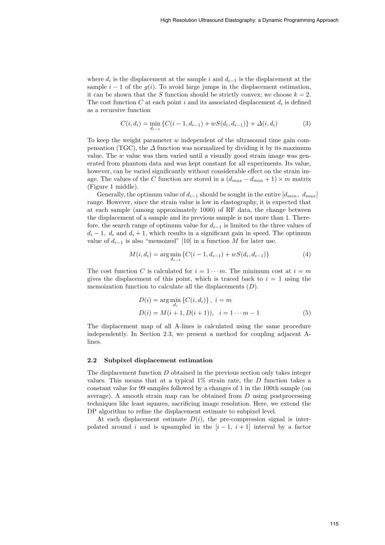
where di is the displacement at the sample i and di−1 is the displacement at thesample i − 1 of the g(i). To avoid large jumps in the displacement estimation,it can be shown that the S function should be strictly convex; we choose k = 2.The cost function C at each point i and its associated displacement di is definedas a recursive function
C(i, di) = mindi−1
{C(i− 1, di−1) + wS(di, di−1)}+Δ(i, di) (3)
To keep the weight parameter w independent of the ultrasound time gain com-pensation (TGC), the Δ function was normalized by dividing it by its maximumvalue. The w value was then varied until a visually good strain image was gen-erated from phantom data and was kept constant for all experiments. Its value,however, can be varied significantly without considerable effect on the strain im-age. The values of the C function are stored in a (dmax − dmin + 1)×m matrix(Figure 1 middle).
Generally, the optimum value of di−1 should be sought in the entire [dmin, dmax]range. However, since the strain value is low in elastography, it is expected thatat each sample (among approximately 1000) of RF data, the change betweenthe displacement of a sample and its previous sample is not more than 1. There-fore, the search range of optimum value for di−1 is limited to the three values ofdi − 1, di and di + 1, which results in a significant gain in speed. The optimumvalue of di−1 is also “memoized” [10] in a function M for later use.
M(i, di) = arg mindi−1
{C(i− 1, di−1) + wS(di, di−1)} (4)
The cost function C is calculated for i = 1 · · ·m. The minimum cost at i = m
gives the displacement of this point, which is traced back to i = 1 using thememoization function to calculate all the displacements (D).
D(i) = argmindi
{C(i, di)} , i = m
D(i) = M(i+ 1, D(i+ 1)), i = 1 · · ·m− 1 (5)
The displacement map of all A-lines is calculated using the same procedureindependently. In Section 2.3, we present a method for coupling adjacent A-lines.
2.2 Subpixel displacement estimation
The displacement function D obtained in the previous section only takes integervalues. This means that at a typical 1% strain rate, the D function takes aconstant value for 99 samples followed by a changes of 1 in the 100th sample (onaverage). A smooth strain map can be obtained from D using postprocessingtechniques like least squares, sacrificing image resolution. Here, we extend theDP algorithm to refine the displacement estimate to subpixel level.
At each displacement estimate D(i), the pre-compression signal is inter-polated around i and is upsampled in the [i− 1, i+ 1] interval by a factor
High Resolution Ultrasound Elastography: a Dynamic Programming Approach
115
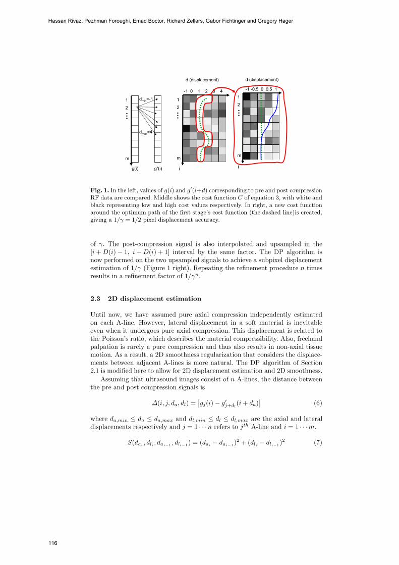
i
d (displacement)
i
-1 -0.5 0 0.5 1
m
1
2
-1 0 1 2 3 4
d (displacement)
m
1
2
g(i)
dmin=-1
dmax=4
g’(i)
m
1
2
Fig. 1. In the left, values of g(i) and g′(i+d) corresponding to pre and post compressionRF data are compared. Middle shows the cost function C of equation 3, with white andblack representing low and high cost values respectively. In right, a new cost functionaround the optimum path of the first stage’s cost function (the dashed line)is created,giving a 1/γ = 1/2 pixel displacement accuracy.
of γ. The post-compression signal is also interpolated and upsampled in the[i+D(i)− 1, i+D(i) + 1] interval by the same factor. The DP algorithm isnow performed on the two upsampled signals to achieve a subpixel displacementestimation of 1/γ (Figure 1 right). Repeating the refinement procedure n timesresults in a refinement factor of 1/γn.
2.3 2D displacement estimation
Until now, we have assumed pure axial compression independently estimatedon each A-line. However, lateral displacement in a soft material is inevitableeven when it undergoes pure axial compression. This displacement is related tothe Poisson’s ratio, which describes the material compressibility. Also, freehandpalpation is rarely a pure compression and thus also results in non-axial tissuemotion. As a result, a 2D smoothness regularization that considers the displace-ments between adjacent A-lines is more natural. The DP algorithm of Section2.1 is modified here to allow for 2D displacement estimation and 2D smoothness.
Assuming that ultrasound images consist of n A-lines, the distance betweenthe pre and post compression signals is
Δ(i, j, da, dl) =∣∣gj(i)− g′
j+dl(i+ da)
∣∣ (6)
where da,min ≤ da ≤ da,max and dl,min ≤ dl ≤ dl,max are the axial and lateraldisplacements respectively and j = 1 · · ·n refers to jth A-line and i = 1 · · ·m.
S(dai, dli , dai−1 , dli−1) = (dai
− dai−1)2 + (dli − dli−1)
2 (7)
Hassan Rivaz, Pezhman Foroughi, Emad Boctor, Richard Zellars, Gabor Fichtinger and Gregory Hager
116

width (mm)
dept
h (m
m)
0 10 20 30
0
5
10
15
20
25
30
(a)
width (mm)
dept
h (m
m)
t
b
b
0 10 20 30
0
5
10
15
20
25
300
0.01
0.02
0.03
0.04
(b)
width (mm)
dept
h (m
m)
t
b
b
0 10 20 30
0
5
10
15
20
25
30
0.01
0.02
0.03
0.04
(c)
width (mm)
dept
h (m
m)
t
b
b
0 10 20 30
0
5
10
15
20
25
300
0.01
0.02
0.03
0.04
(d)
width (mm)
dept
h (m
m)
t
b
b
0 10 20 30
0
5
10
15
20
25
30 0
0.05
0.1
0.15
0.2
0.25
(e)
width (mm)
dept
h (m
m)
t
b
b
0 10 20 30
0
5
10
15
20
25
30 0
0.05
0.1
0.15
0.2
0.25
(f)
Fig. 2. B-mode image (a) and elastograms obtained from freehand palpation of thebreast elastography phantom using cross correlation (b), 1D DP (c), 2D DP (d), crosscorrelation with B-mode data (e) and 1D DP with B-mode data (f). The rectanglesshow CNR calculation windows (t and b refer to target and background).
is the smoothness regularization with subscripts a and l referring to axial andlateral. The cost function at the ith sample of the jth A-line is
Cj(da, dl, i) = minδa,δl
{Cj(δa, δl, i− 1) + Cj−1(δa, δl, i)
2+ wS(da, dl, δa, δl)
}+ Δ(da, dl, i) (8)
For memoization, δa and δl values that minimize the cost function are stored forall da, dl and i values. The specific form of the cost function allows the calculationof the displacement of each A-line using the cost values of the previous A-line.The cost function of the jth line, Cj(da, dl, i), is calculated and is minimized,resulting in its displacement map. The Cj(da, dl, i) function is also used forthe calculation of the next cost function Cj+1(da, dl, i) and is deleted from thememory afterwards. This makes the amount of memory required to store thecost function values independent of the number of A-lines.
3 Results and Discussion
RF data was acquired from an Antares Siemens system (Issaquah, WA) with a7.27MHz linear array at a sampling rate of 40MHz. For comparison, strain im-
High Resolution Ultrasound Elastography: a Dynamic Programming Approach
117
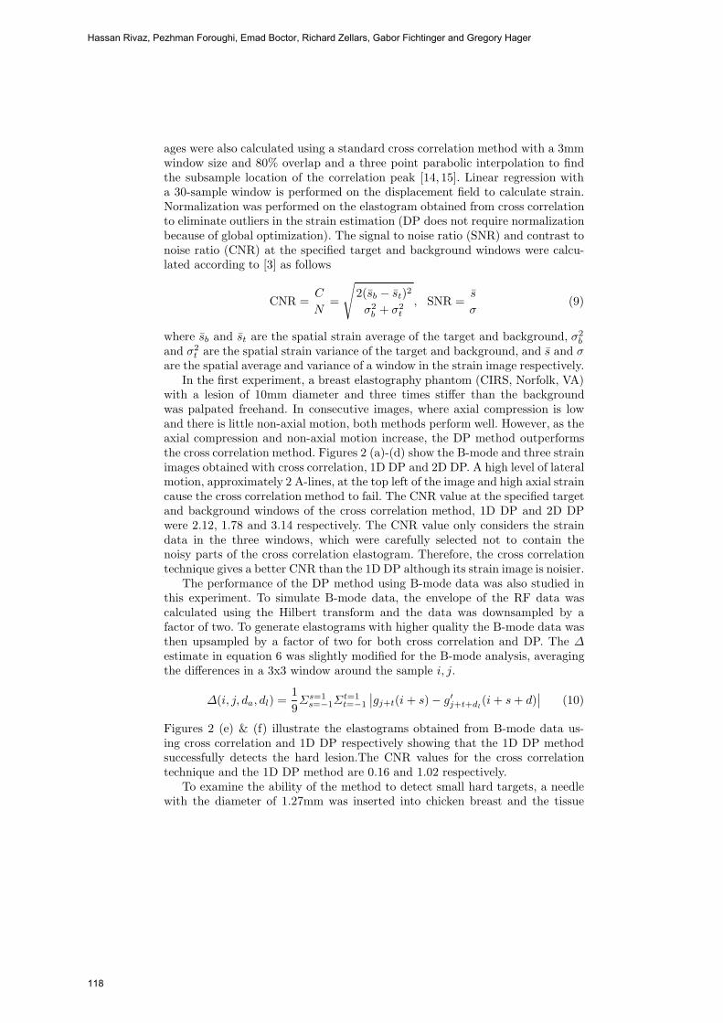
ages were also calculated using a standard cross correlation method with a 3mmwindow size and 80% overlap and a three point parabolic interpolation to findthe subsample location of the correlation peak [14, 15]. Linear regression witha 30-sample window is performed on the displacement field to calculate strain.Normalization was performed on the elastogram obtained from cross correlationto eliminate outliers in the strain estimation (DP does not require normalizationbecause of global optimization). The signal to noise ratio (SNR) and contrast tonoise ratio (CNR) at the specified target and background windows were calcu-lated according to [3] as follows
CNR =C
N=
√2(sb − st)2
σ2b + σ2
t
, SNR =s
σ(9)
where sb and st are the spatial strain average of the target and background, σ2b
and σ2t are the spatial strain variance of the target and background, and s and σ
are the spatial average and variance of a window in the strain image respectively.In the first experiment, a breast elastography phantom (CIRS, Norfolk, VA)
with a lesion of 10mm diameter and three times stiffer than the backgroundwas palpated freehand. In consecutive images, where axial compression is lowand there is little non-axial motion, both methods perform well. However, as theaxial compression and non-axial motion increase, the DP method outperformsthe cross correlation method. Figures 2 (a)-(d) show the B-mode and three strainimages obtained with cross correlation, 1D DP and 2D DP. A high level of lateralmotion, approximately 2 A-lines, at the top left of the image and high axial straincause the cross correlation method to fail. The CNR value at the specified targetand background windows of the cross correlation method, 1D DP and 2D DPwere 2.12, 1.78 and 3.14 respectively. The CNR value only considers the straindata in the three windows, which were carefully selected not to contain thenoisy parts of the cross correlation elastogram. Therefore, the cross correlationtechnique gives a better CNR than the 1D DP although its strain image is noisier.
The performance of the DP method using B-mode data was also studied inthis experiment. To simulate B-mode data, the envelope of the RF data wascalculated using the Hilbert transform and the data was downsampled by afactor of two. To generate elastograms with higher quality the B-mode data wasthen upsampled by a factor of two for both cross correlation and DP. The Δ
estimate in equation 6 was slightly modified for the B-mode analysis, averagingthe differences in a 3x3 window around the sample i, j.
Δ(i, j, da, dl) =19Σs=1s=−1Σ
t=1t=−1
∣∣gj+t(i + s)− g′
j+t+dl(i+ s+ d)
∣∣ (10)
Figures 2 (e) & (f) illustrate the elastograms obtained from B-mode data us-ing cross correlation and 1D DP respectively showing that the 1D DP methodsuccessfully detects the hard lesion.The CNR values for the cross correlationtechnique and the 1D DP method are 0.16 and 1.02 respectively.
To examine the ability of the method to detect small hard targets, a needlewith the diameter of 1.27mm was inserted into chicken breast and the tissue
Hassan Rivaz, Pezhman Foroughi, Emad Boctor, Richard Zellars, Gabor Fichtinger and Gregory Hager
118

width (mm)
dept
h (m
m)
0 10 20 30
0
5
10
15
(a)
width (mm)
dept
h (m
m)
0 10 20 30
0
5
10
15 −0.05
0
0.05
0.1
(b)
width (mm)
dept
h (m
m)
0 10 20 30
0
5
10
15
−0.05
0
0.05
0.1
(c)Fig. 3. B-mode image (a) and elastograms obtained from freehand palpation of the invitro chicken breast with an inserted needle using cross correlation (b), and 2D DP(c) . The needle is marked by a circle (appearing as an ellipse because of the scalingratios). The large strain value over the needle indicates stress concentration.
was palpated freehand. In Figure 3(a), the B-mode image of the tissue is shown;the circle in the three images of Figure 3, whose center is located manuallyfrom the B-mode image, marks the needle. Elastograms obtained using the crosscorrelation and 2D DP techniques are shown in Figures 3 (b) & (c) respectively.High values of strain (white regions) can be observed over the needle in the 2DDP elastogram indicating stress concentration caused by the hard needle.
0 0.005 0.01 0.015 0.02 0.025 0.03 0.035 0.040
10
20
30
40
50
strain
SN
R
cross corr.1D DP2D DP
Fig. 4. SNR values of the crosscorrelation, 1D DP and 2D DPtechniques (dashed, dotted andsolid curves respectively).
A CIRS elasticity QA phantom with a10mm diameter lesion and with the lesionand background Young’s elasticity moduleof 25 kPa and 33kPa respectively was com-pressed in 24 steps (each step 0.005in). Thestrain map between the first frame and allother frame was calculated using the crosscorrelation and DP methods. The SNR met-ric was calculated in a small window locatedat the top center of the image, where strain isapproximately constant. Figure 4 shows thatthe DP methods have higher dynamic range,an important elastography performance metric [3]. Since the 1D DP method cal-culates the displacement at subpixel level, it gives higher SNR at small strainsthan the 2D DP. This indicates the importance of subpixel displacement es-timation for small compression. Implementation of the subpixel displacementestimation for the 2D DP method is underway.
Substituting other computationally more expensive similarity measures likesum of square difference and normalized cross correlation in the Δ function re-sulted in no significant difference in the performance. Currently, an elastogram of1000x100 pixels with maximum axial displacement of 10 samples (1% strain) andmaximum lateral displacement of ±1 A-lines takes 1.4sec to generate; 0.25secfor calculating the Δ function and 1.1sec for the DP optimization (on a 3.8GHzP4 CPU). Current implementation is in MATLAB with the Δ function calcu-
High Resolution Ultrasound Elastography: a Dynamic Programming Approach
119
lation and the DP optimization in mex functions. If the organ is palpated withthe probe, the displacement of the parts of the image close to the probe is verysmall. Taking advantage of this will result in increasing the speed by a factorof 2. Also a hierarchical search, similar to the subpixel displacement estimationof Section 2.2, and exploiting hardware parallelism can significantly speed thealgorithm.
4 Conclusion and Future Work
An elastography algorithm that is significantly more robust to the signal decor-relation (caused by scatterer motion in high axial compression, and lateral andout of plane motions of the probe) than cross correlation techniqes is presented.This allows higher axial compression, increasing the dynamic range of the elas-togram which is crucial for lesion detection. The CNR and SNR metrics seemto indicate that the regularization creates smooth elastograms while preservingcontrast. The regularization also does not appear to damage the ability of thealgorithm to detect small targets, like the small Brachytherapy needle. Furtherwork is required to study the effect of regularization on the contrast. Futurework will study the effect of uncontrolled tissue motion such as blood flow andrespiration on the DP algorithm. The 2D algorithm can be extended to 2D+t,to exploit the cost function in previous time as well as incorporating a 2D+tsmoothness regularization.
References
1. Garra, B., Cespedes, E., Ophir, J., Spratt, S., Zuurbier, R., Magnant, C., Pennanen,M.: Elastography of breast lesions: initial clinical results. Radiology 202 (1997)79–86
2. Varghese, T., Zagzebski, J., Lee, F.: Elastographic imaging of thermal lesions inthe liver in vivo following radiofrequency ablation: preliminary results. UMB 28(2002) 1467–1473
3. Ophir, J., Alam, S., Garra, B., Kallel, F., Konofagou, E., Krouskop, T., Varghese,T.: Elastography: ultrasonic estimation and imaging of the elastic properties oftissues. Annu. Rev. Biomed. Eng. 213 (1999) 203–233
4. Greenleaf, J., Fatemi, M., Insana, M.: Selected methods for imaging elastic prop-erties of biological tissues. Annu. Rev. Biomed. Eng. 5 (2003) 5778
5. Lindop, J., Treece, G., Gee, A., Prager, R.: Dynamic resolution selection in ultra-sonic strain imaging. Univ. Cambridge Tech. Rep. (2006) 1–25
6. Varghese, T., Ophir, J.: Enhancement of echo-signal correlation in elastographyusing temporal stretching. IEEE T. UFFC 44 (1997) 173–180
7. Chaturvedi, P., Insana, M., Hall, T.: 2-d companding for noise reduction in strainimaging. IEEE T. UFFC 45 (1998) 179–191
8. Walker, W., Trahey, G.: A fundamental limit on delay estimation using partiallycorrelated speckle signals. IEEE T. UFFC 42 (1995) 301–308
9. Pellot-Barakat, C., Frouin, F., Insana, M., Herment, A.: Ultrasound elastographybased on multiscale estimations of regularized displacement fields. IEEE TMI (04)
10. Bellman, R.: Applied dynamic programming. Princeton Univ. Press (1962)
Hassan Rivaz, Pezhman Foroughi, Emad Boctor, Richard Zellars, Gabor Fichtinger and Gregory Hager
120

11. Ohta, Y., Kanade, T.: Stereo by intra- and inter-scanline search using dynamicprogramming. IEEE PAMI 7 (1985) 139–154
12. Geiger, D., Gupta, A., Costa, L., Vlontzos, J.: Dynamic programming for detecting,tracking, and matching deformable contours. IEEE PAMI 17 (1995) 294–302
13. Sakoe, H., Chiba, S.: Dynamic programming algorithm optimization for spokenword recognition. IEEE T. Sig. Proc 26 (1978) 43–49
14. Cespedes, I., Huang, Y., Ophir, J., Spratt, S.: Methods for estimation of subsampletime delays of digitized echo signals. Ultrason. Imag. 17 (1995) 142–171
15. Zahiri, R., Salcudean, S.: Motion estimation in ultrasound images using timedomain cross correlation with prior estimates. IEEE T. Biomed. Eng. 53 (2006)
High Resolution Ultrasound Elastography: a Dynamic Programming Approach
121

Multi-resolution 3D Nonrigid Registration viaOptimal Mass Transport on the GPU
Tauseef ur Rehman1, Gallagher Pryor2, John Melonakos1, and AllenTannenbaum1
1 School of Electrical and Computer Engineering, Georgia Institute of Technology,Atlanta, GA tauseef,jmelonak,[email protected],
2 College of Computing, Georgia Institute of Technology, Atlanta, [email protected]
Abstract. In this paper we present computationally efficient imple-mentation of the minimizing flow approach for optimal mass transport(OMT) with applications to non-rigid 3D image registration. Our imple-mentation solves the OMT problem via multi-resolution, multigrid, andparallel methodologies on a consumer graphics processing unit (GPU).Although computing the optimal map has shown to be computationallyexpensive in the past, we show that our approach is almost two ordersmagnitude faster than previous work and is capable of finding transportmaps with optimality measures (mean curl) previously unattainable byother works (which directly influences the accuracy of registration). Wegive results where the algorithm was used to compute non-rigid regis-trations of 3D synthetic data as well as intra-patient pre-operative andpost-operative 3D brain MRI datasets.
1 Introduction
Image registration and morphing are amongst the most common image process-ing problems. Registration is the process of establishing a common geometricreference frame between two or more image data sets and is necessary in or-der to compare or integrate image data obtained from different measurements.A vast amount of literature exists on image registration techniques and we re-fer the reader to [1, 2] for an overview of this field. In this paper, we approachthe registration task by treating it as an optimal mass transport problem. Aswith other registration techniques, the computational burden associated withthis problem is high. We propose a multi-resolution approach for the solution ofthis problem on the GPU to alleviate this difficulty.
The optimal mass transport problem was first formulated by a French math-ematician Gasper Monge in 1781, and was given a modern formulation in thework of Kantorovich [3] and, therefore, is now known as the Monge-Kantorovichproblem. The original problem concerned finding the optimal way to move a pileof soil from one site to another in the sense of minimal transportation cost.Hence, the Kantorovich-Wasserstein distance is also commonly referred to asthe Earth Mover’s Distance (EMD).
122
Recently, Haker et al. [4, 5] have applied the optimal mass transport approachto certain medical image registration problems. Rigorous mathematical detailsfor their algorithm are given by Angenent et al. [6]. Although there have beena number of algorithms in the literature for computing an optimal mass trans-port, the method by Haker et al. computes the optimal warp from a first orderpartial differential equation, which is a computational improvement over earlierproposed higher order methods and computationally complex discrete methodsbased on linear programming. However, at large grid sizes and especially for 3Dregistration the computational cost of even this method is significant.
Though computationally expensive, the OMT method has a number of dis-tinguishing characteristics: (1) it is a parameter free method and no landmarksneed be specified, (2) it is symmetrical (the mapping from image A to image Bis the inverse of the mapping from B to A), (3) its solution is unique (no localminima), (4) it can register images where brightness constancy is an invalidassumption, and (5) OMT is specifically designed to take into account changesin densities that result from changes in area or volume.
Contribution. In this paper we extend our previous work [7] and implementthe more general formulation of the OMT problem for 3D non-rigid registrationbased on multi-resolution techniques and using the parallel architecture of theGPU. Although multi-resolution methods have served as critical pieces of reg-istration algorithms in the past, it had yet to be shown that the Optimal MassTransport problem could be solved in the same manner. Our experimental re-sults show that this is indeed the case, a result which has implications for manyfields beyond imaging due to the ubiquitous nature of the OMT problem. Wealso show that the PDE-based solution to the OMT problem is greatly enhancedby our approach to such an extent that it becomes practical for use on large 3Ddatasets both in terms of speed and accuracy. Overall, these results show thatOMT-based image registration is practical on medical imagery and, thus, mer-its further investigation as an elastic registration technique without the need ofsmoothness priors or brightness constancy assumptions.
2 Optimal Mass Transport for Registration
2.1 Formulation of the Problem
We will briefly provide an introduction to the modern formulation of the Monge-Kantorovich problem. We assume we are given, a priori, two sub-domains Ω0 andΩ1 of Rd with smooth boundaries, and a pair of positive density functions, μ0
and μ1 defined on Ω0 and Ω1 respectively. We assume that,∫Ω0
μ0 =∫Ω1
μ1 (1)
This ensures that we have same total mass in both the domains. The functionsμ0 and μ1 in this formulation can be the same as the source and target images,respectively, or a smooth version of them. They can also be scalar fields that are
Multi-resolution 3D Nonrigid Registration via Optimal Mass Transport on the GPU
123

appropriate for the underlying physical model. We now consider diffeomorphismsu from Ω0 to Ω1 which map one density to other in the sense that,
μ0 = |Du|μ1 ◦ u (2)
which we call the mass preservation (MP) property, and write u ∈ MP . Equa-tion (2) is called the Jacobian equation. Here, |Du| denotes the determinantof the Jacobian map Du, and ◦ denotes composition of functions. It basicallyimplies that if a small region in Ω0 is mapped to a larger region in Ω1, thenthere must be a corresponding decrease in density in order for the mass to bepreserved. There may be many such mappings, and we want to pick an optimalone in some sense. Accordingly, we define the squared L2 Monge-Kantorovichdistance as following:
d22(μ0, μ1) = infu∈MP
∫Ω0
‖ u(x) − x ‖2 μ0(x)dx (3)
The optimal MP map is a map which minimizes this integral while satisfyingthe constraint given by Equation (2). The Monge-Kantorovich functional, Equa-tion (3), is seen to place a penalty on the distance the map u moves each bit ofmaterial, weighted by the material’s mass. A fundamental theoretical result [8,9], is that there is a unique optimal u ∈MP transporting μ0 to μ1, and that uis characterized as the gradient of a convex function ω, i.e., u = ∇ω. This theorytranslates into a practical advantage, since it means that there are no non-globalminima to stall our solution process.
2.2 Computing the Transport Map
We will describe here only the algorithm for finding the optimal mapping u.The details of this method can be found in [4]. The basic idea for finding theoptimal warping function is first to find an initial MP mapping u0 and update ititeratively to decrease an energy functional. When the pseudo time t goes to ∞,the optimal u will be found, which is u. Basically there are two steps. The firststep in this algorithm is to find an initial mass preserving mapping. This canbe done for general domains using the method of Moser [10] or the algorithmproposed in [4]. The later method can simply be interpreted as the solutionof a one-dimensional Monge-Kantorovich problem in the x-direction followedby the solution of a family of one-dimensional Monge-Kantorovich problems iny-direction and finally solve a family of 2D Monge-Kantorovich problems inthe z-direction. The second step is to adjust the initial mapping found aboveiteratively using gradient descent in order to minimize the functional defined inEquation (3), while constraining u so that it continues to satisfy Equation (2).This process iteratively removes the curl from the initial mapping u and, thereby,finds the polar factorization of u. For details on this technique, please refer to[4]. The overall algorithm is summarized graphically in Figure 1. This samealgorithm can be used to compute transport map in arbitrary dimensions theonly difference being that in R2 the problem is a bit simpler where you solve
Tauseef ur Rehman, Gallagher Pryor, John Melonakos, and Allen Tannenbaum
124
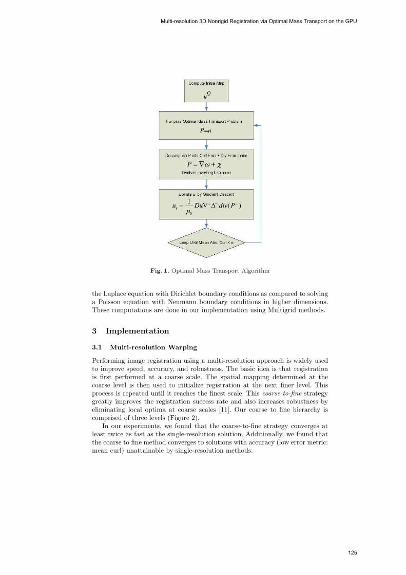
Fig. 1. Optimal Mass Transport Algorithm
the Laplace equation with Dirichlet boundary conditions as compared to solvinga Poisson equation with Neumann boundary conditions in higher dimensions.These computations are done in our implementation using Multigrid methods.
3 Implementation
3.1 Multi-resolution Warping
Performing image registration using a multi-resolution approach is widely usedto improve speed, accuracy, and robustness. The basic idea is that registrationis first performed at a coarse scale. The spatial mapping determined at thecoarse level is then used to initialize registration at the next finer level. Thisprocess is repeated until it reaches the finest scale. This coarse-to-fine strategygreatly improves the registration success rate and also increases robustness byeliminating local optima at coarse scales [11]. Our coarse to fine hierarchy iscomprised of three levels (Figure 2).
In our experiments, we found that the coarse-to-fine strategy converges atleast twice as fast as the single-resolution solution. Additionally, we found thatthe coarse to fine method converges to solutions with accuracy (low error metric:mean curl) unattainable by single-resolution methods.
Multi-resolution 3D Nonrigid Registration via Optimal Mass Transport on the GPU
125

Fig. 2. A Multi-Resolution Registration Scheme. We employ a coarse to finehierarchy three levels deep with which we solve for an optimal mapping from sourceto destination data. This method has shown to speed convergence and realize moreaccurate solutions.
3.2 3D Multigrid Laplacian Inversion
We inverted the Laplacian (a key component of the OMT algorithm) using a 3Dmultigrid solver. The multigrid idea is very fundamental, it takes advantage ofthe smoothing properties of the classical iteration methods at high frequencies(Jacobi, Gauss Siedel, SOR etc) and the error smoothing at low frequencies byrestriction to coarse grids. The essential multigrid principle is to approximatethe smooth (low frequency) part of the error on coarser grids. The non-smoothor rough part is reduced with a small number of iterations with a basic iterativemethod on the fine grid.
The basic components of multigrid algorithm are discretization, intergridtransfer operators (interpolation & restriction), relaxation scheme and the iter-ative cycling structure. We used an explicit finite difference scheme for approxi-mating the 3D Poisson equation. This approach uses a 19-point formula on theuniform cubic grid. Relaxation was performed using a parallelizable four-colorGauss-Seidel relaxation scheme. This increases robustness and efficiency and isespecially suited for the implementation on the GPU. We used tri-linear interpo-lation operator for transferring coarse grid correction to fine grids. The residualrestriction operator for projecting residual from the fine to coarse grids is thefull-weighting scheme. A multigrid V(2,2)-cycle algorithm was used to iterate forsolution (Residual max norm ≈ 10−5). Interested readers are referred to [12–14]for details on implementation of the multigrid methods.
3.3 GPU Implementation
An advantage of our solution to the OMT problem is that it is particularly suitedfor implementation on parallel computing architectures. Over the past few years,it has been shown that graphics processing units (GPUs; now standard in most
Tauseef ur Rehman, Gallagher Pryor, John Melonakos, and Allen Tannenbaum
126
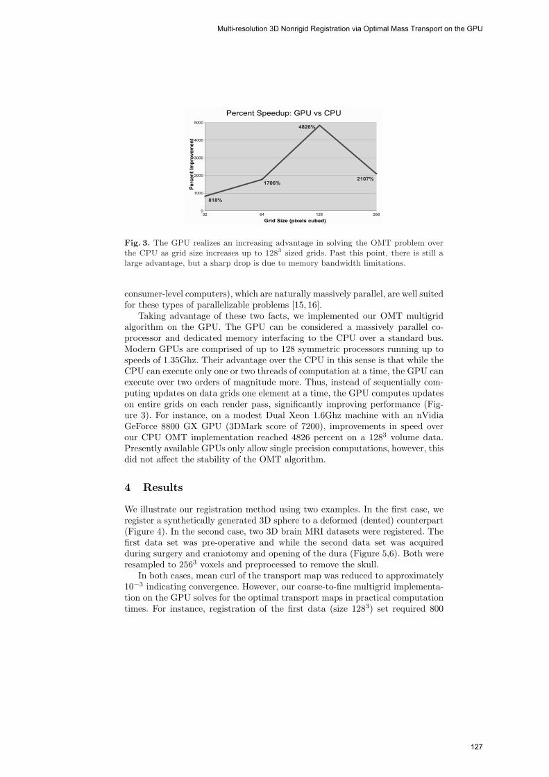
Fig. 3. The GPU realizes an increasing advantage in solving the OMT problem overthe CPU as grid size increases up to 1283 sized grids. Past this point, there is still alarge advantage, but a sharp drop is due to memory bandwidth limitations.
consumer-level computers), which are naturally massively parallel, are well suitedfor these types of parallelizable problems [15, 16].
Taking advantage of these two facts, we implemented our OMT multigridalgorithm on the GPU. The GPU can be considered a massively parallel co-processor and dedicated memory interfacing to the CPU over a standard bus.Modern GPUs are comprised of up to 128 symmetric processors running up tospeeds of 1.35Ghz. Their advantage over the CPU in this sense is that while theCPU can execute only one or two threads of computation at a time, the GPU canexecute over two orders of magnitude more. Thus, instead of sequentially com-puting updates on data grids one element at a time, the GPU computes updateson entire grids on each render pass, significantly improving performance (Fig-ure 3). For instance, on a modest Dual Xeon 1.6Ghz machine with an nVidiaGeForce 8800 GX GPU (3DMark score of 7200), improvements in speed overour CPU OMT implementation reached 4826 percent on a 1283 volume data.Presently available GPUs only allow single precision computations, however, thisdid not affect the stability of the OMT algorithm.
4 Results
We illustrate our registration method using two examples. In the first case, weregister a synthetically generated 3D sphere to a deformed (dented) counterpart(Figure 4). In the second case, two 3D brain MRI datasets were registered. Thefirst data set was pre-operative and while the second data set was acquiredduring surgery and craniotomy and opening of the dura (Figure 5,6). Both wereresampled to 2563 voxels and preprocessed to remove the skull.
In both cases, mean curl of the transport map was reduced to approximately10−3 indicating convergence. However, our coarse-to-fine multigrid implementa-tion on the GPU solves for the optimal transport maps in practical computationtimes. For instance, registration of the first data (size 1283) set required 800
Multi-resolution 3D Nonrigid Registration via Optimal Mass Transport on the GPU
127
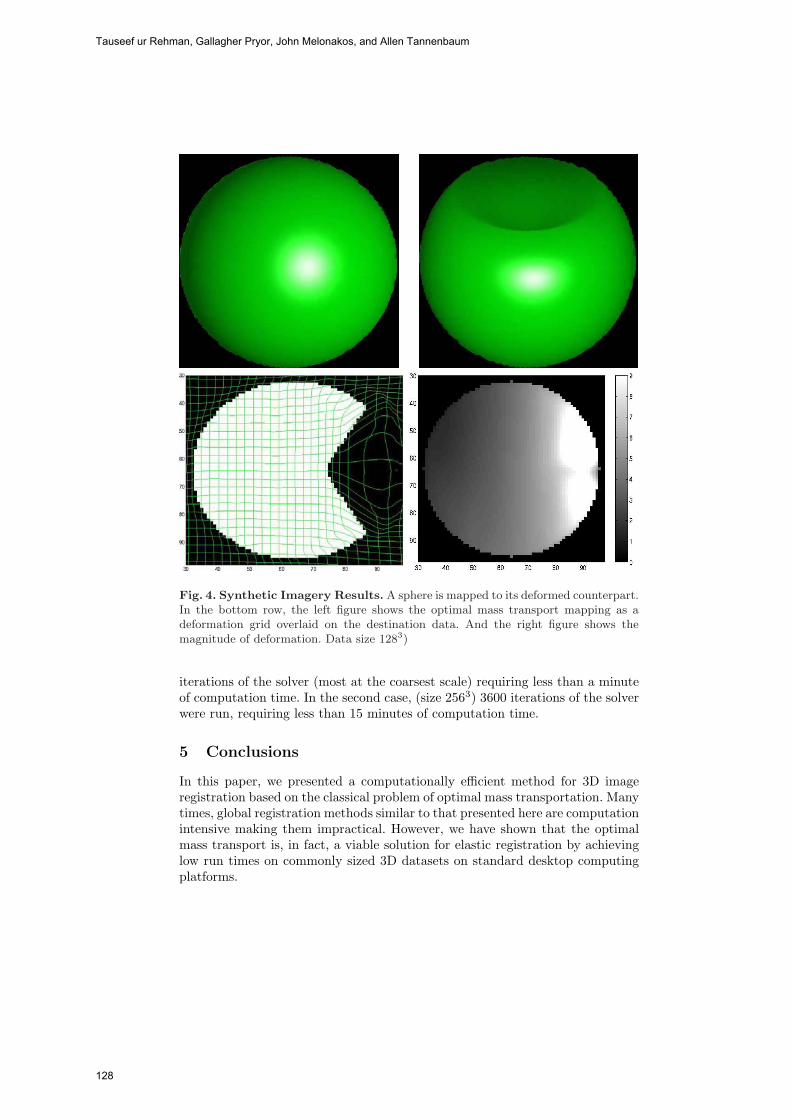
Fig. 4. Synthetic Imagery Results. A sphere is mapped to its deformed counterpart.In the bottom row, the left figure shows the optimal mass transport mapping as adeformation grid overlaid on the destination data. And the right figure shows themagnitude of deformation. Data size 1283)
iterations of the solver (most at the coarsest scale) requiring less than a minuteof computation time. In the second case, (size 2563) 3600 iterations of the solverwere run, requiring less than 15 minutes of computation time.
5 Conclusions
In this paper, we presented a computationally efficient method for 3D imageregistration based on the classical problem of optimal mass transportation. Manytimes, global registration methods similar to that presented here are computationintensive making them impractical. However, we have shown that the optimalmass transport is, in fact, a viable solution for elastic registration by achievinglow run times on commonly sized 3D datasets on standard desktop computingplatforms.
Tauseef ur Rehman, Gallagher Pryor, John Melonakos, and Allen Tannenbaum
128
Acknowledgements
This work was supported in part by grants from NSF, AFOSR, ARO, MURI,MRI-HEL as well as by a grant from NIH (NAC P41 RR-13218) through Brighamand Women’s Hospital. This work is part of the National Alliance for Medi-cal Image Computing (NAMIC), funded by the National Institutes of Healththrough the NIH Roadmap for Medical Research, Grant U54 EB005149. Infor-mation on the National Centers for Biomedical Computing can be obtained fromhttp://nihroadmap.nih.gov/bioinformatics.
References
1. Maintz, J.A., Viergever, M.A.: A survey of medical image registration. MedicalImage Analysis 2 (1998) 1–57
2. Brown, L.G.: A survey of medical image registration. ACM Computing Surveys24 (1992) 325–376
3. Kantorovich, L.V.: On a problem of monge. Uspekhi Matematicheskikh Nauk. 3(1948) 225–226
4. S.Haker, Zhu, L., Tannenbaum, A., Angenent, S.: Optimal mass transport forregistration and warping. International Journal of Computer Vision 60(3) (2004)225–240
5. S.Haker, Tannenbaum, A., Kikinis, R.: Mass preserving mappings and image reg-istration. In: MICCAI. (2001) 120–127
6. Angenent, S., Haker, S., Tannenbaum, A.: Minimizing flows for the monge-kantorovich problem. SIAM Journal of Mathematical Analysis 36 (2003) 61–97
7. Rehman, T., Tannenbaum, A.: Multigrid optimal mass transport for image reg-istration and morphing. In: Proceedings of SPIE Conference on ComputationalImaging V. Volume 6498. (2007)
8. Brenier, Y.: Polar factorization and monotone rearrangement of vector-valuedfunctions. Communications on Pure and Applied Mathematics 64 (1991) 375–417
9. Gangbo, W., McCann, R.: The geometry of optimal transportation. Acta Mathe-matica 177 (1996) 113–161
10. Moser, J.: On the volume elements on a manifold. Transactions of the AmericanMathematical Society 120 (1965) 286–294
11. Yoo, T.S.: Insight into Images, Principles and Practice for Segmentation, Regis-tration and Image Analysis. A. K. Peters Ltd. 2004 (2004)
12. Gupta, M.M., Zhang, J.: High accuracy multigrid solution of the 3d convection-diffusion equation. Applied Mathematics and Computation 113 (2000) 249–274
13. W.L.Briggs, Hensen, V., McCormick, S.: A Multigrid Tutorial. SIAM (2000)14. Trottenberg, U., Oosterelee, C., Schuller, A.: A Multigrid Tutorial. SIAM (2000)15. Bolz, J., et al.: Sparse matrix solvers on the GPU: Conjugate gradients and multi-
grid. In: Proceedings of SIGGRAPH. Volume 22. (2003) 917–92416. Nolan, G., et al.: A multigrid solver for boundary value problems using pro-
grammable graphics hardware. In: Proceedings of SIGGRAPH. (2003) 102–111
Multi-resolution 3D Nonrigid Registration via Optimal Mass Transport on the GPU
129
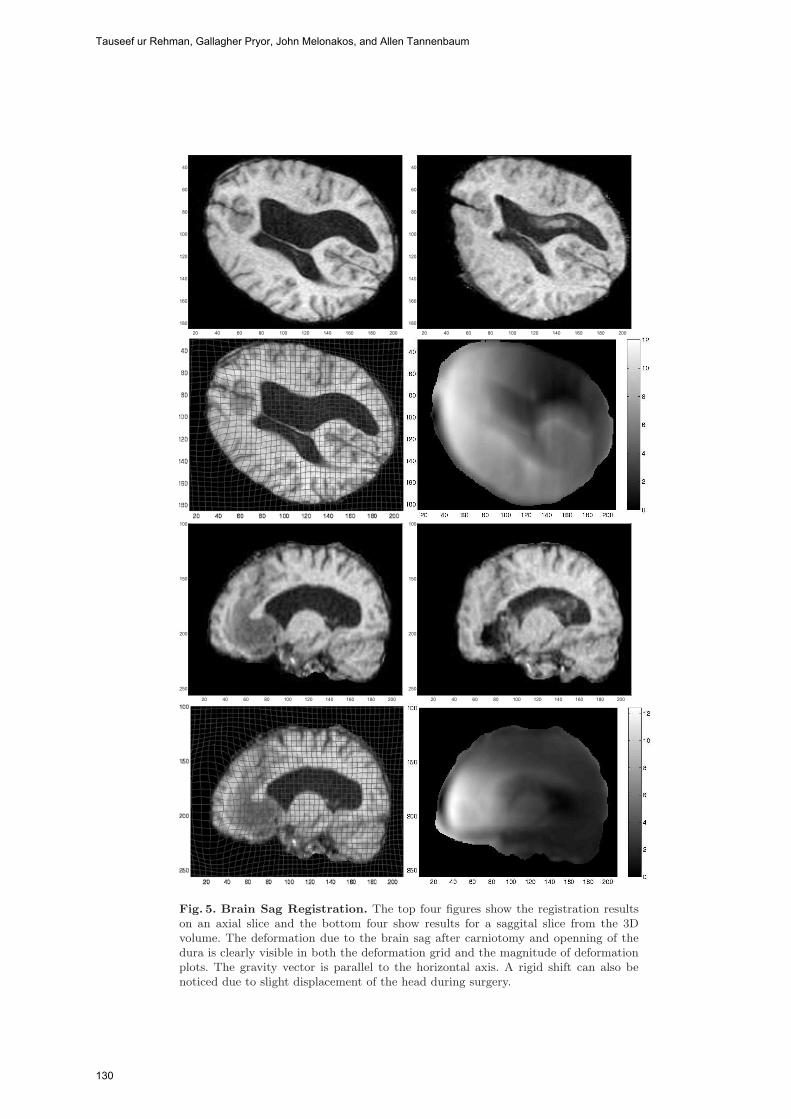
20 40 60 80 100 120 140 160 180 200
40
60
80
100
120
140
160
180
20 40 60 80 100 120 140 160 180 200
40
60
80
100
120
140
160
180
20 40 60 80 100 120 140 160 180 200
100
150
200
250
20 40 60 80 100 120 140 160 180 200
100
150
200
250
Fig. 5. Brain Sag Registration. The top four figures show the registration resultson an axial slice and the bottom four show results for a saggital slice from the 3Dvolume. The deformation due to the brain sag after carniotomy and openning of thedura is clearly visible in both the deformation grid and the magnitude of deformationplots. The gravity vector is parallel to the horizontal axis. A rigid shift can also benoticed due to slight displacement of the head during surgery.
Tauseef ur Rehman, Gallagher Pryor, John Melonakos, and Allen Tannenbaum
130
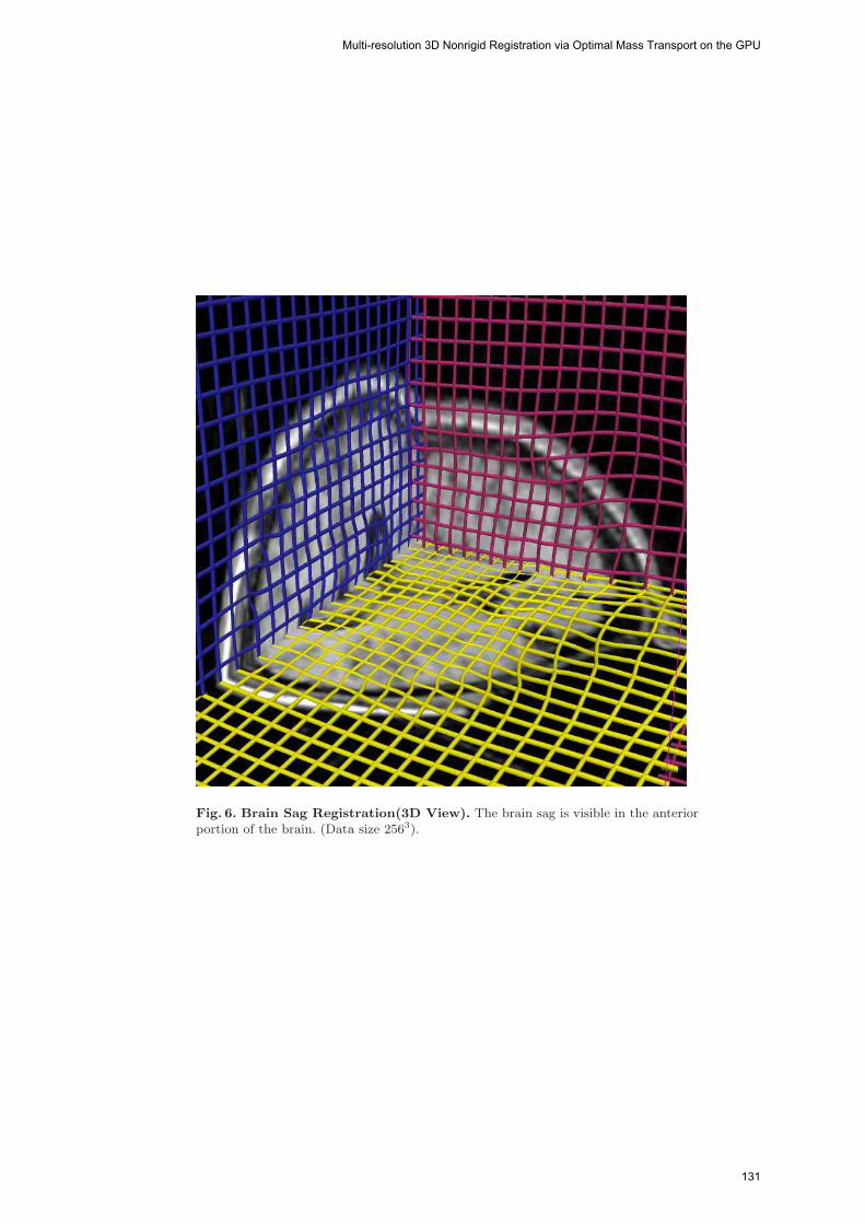
Fig. 6. Brain Sag Registration(3D View). The brain sag is visible in the anteriorportion of the brain. (Data size 2563).
Multi-resolution 3D Nonrigid Registration via Optimal Mass Transport on the GPU
131

Part 2
Computational Fluid Mechanics and Thermodynamics
132

Hardware-accelerated Bleeding Simulation forVirtual Surgery
Jing Qin1, Wai-Man Pang1, Yim-Pan Chui1, Yong-Ming Xie1,Tien-Tsin Wong1, Wai-Sang Poon2, Kwok Sui Leung3, Pheng-Ann Heng1,4
1 Dept. of Computer Science and Engineering, The Chinese University of Hong Kong2 Department of Surgery, The Chinese University of Hong Kong
3 Department of Orthopaedics and Traumatology,The Chinese University of Hong Kong
4 Shun Hing Institute of Advanced Engineering,The Chinese University of Hong Kong
Abstract. In this paper, a novel hardware-accelerated framework is pro-posed for real-time and realistic simulation of bleeding. In the frame-work, computational advantage of newly released Physics ProcessingUnit (PPU) is exploited for simulating the mechanical behavior of bloodbased on Smoothed Particle Hydrodynamics (SPH). The realism andflexibility of the framework are achieved by adjusting the biomechani-cal properties of blood and providing proper collision detection betweenblood and soft tissues such as human skin. A GPU-based marching cubesalgorithm is also developed to accelerate the rendering process. Experi-mental results demonstrate our framework can greatly improve the timeperformance of bleeding simulation with satisfying realism and has po-tential to be integrated into many interactive simulators.
1 Introduction
Considerable efforts have been dedicated to improving the performance of com-puter-assisted surgical simulation. While many simulators have been developed,most of them focus on providing interactive deformable models of soft tissuesand rapid haptic rendering. However, real-time and realistic simulation of bleed-ing, which is an important component of virtual surgery, is given relatively littleattention. In reality, bleeding simulation profoundly influences the quality of sur-gical training and planning, since the handling of various bleeding phenomenarequires specific skills from the surgeons. For example, in hysteroscopic simula-tors, some work has been done to simulate the diffusion of intra-uterine bleeding,which should obscure the view of the surgeons in real surgery. The added real-ism can help surgeons learn how to perform correct action in this situation[1].Moreover, bleeding simulation can provide crucial information for surgical train-ing and designing. For example, related information on aneurysm hemodynamicsand pathology can be obtained from bleeding simulation for designing treatmentof aneurysms. Finally, modeling blood flow is not only essential for surgical simu-lation but also in diagnosis and treatment planning of individual patient data[2].
133
The key challenge of real-time bleeding simulation is imitating the behaviorsof blood interactively and accurately with sophisticated viscous fluid modelsand complicated biomechanical properties, but under limitation of computa-tional power. In this paper, a novel framework for real-time bleeding simulationwith hardware acceleration is proposed. In the framework, the computationaladvantage of newly released Physics Processing Unit (PPU) is exploited for sim-ulating the various bleeding phenomena based on Smoothed Particle Hydrody-namics (SPH). To ensure the realism, parameters of vessels are extracted fromChinese Visible Human(CVH) dataset, together with biomechanics of humanblood, to generate the particle-based blood model. Collision detection is imple-mented by constructing proper models based on the built-in algorithm of thePPU. A GPU-based marching cubes algorithm is also developed to acceleratethe rendering process.
2 Previous Work
Different approaches for bleeding simulation have been proposed, which can besummarized into two major categories: temporal texture synthesis and physi-cally based imitation. Although the former can mimic certain phenomena suchas effusion[3], this technique does not have the full capability of synthesizingheterogeneous texture for complicated bleeding phenomena such as flowing andemitting.
In the past, the adoption of physically based methods is limited by the perfor-mance of computational power. The development of computational techniquesin fluid dynamics[4], together with the increasing capability of the hardware,found many promising approaches in vascular and bleeding simulation[5][6]. Ingeneral, these approaches can be categorized into two classes: grid-based meth-ods and particle-based methods.Although some speedup algorithms have beenproposed[7][8], these methods are still not suitable for most real-time and in-teractive surgical simulation, especially when complicated models are used toensure the realism. Smoothed Particle Hydrodynamics (SPH) is one of the effi-cient particle based methods initially proposed for the simulation of astrophysicalproblems such as fission and stars. This technique was first introduced to thecomputer graphics community to depict fire and other gaseous phenomena[9].Muller adopted this method to simulate bleeding for virtual surgery with mod-els of up to 3000 particles[10]. Recently, Daenzer proposed a method to simulatebleeding and smoke in virtual surgery based on simple particle system[11].
3 The Framework
3.1 The Design of Overall Framework
General work-flow of the framework is illustrated in Fig.1. After identifying somenecessary parameters such as the central lines, the radius and the vascular wallthickness of the vessels from the CVH dataset, a particle system is created by amodule named Particles Distributor(PD). Integrating this particle system withbiomechanical properties of blood, a complete blood model represented by an
Jing Qin, Wai-Man Pang, Yim-Pan Chui, Yong-Ming Xie, Tien-Tsin Wong, Wai-Sang Poon, Kwok Sui Leung, Pheng-Ann Heng
134
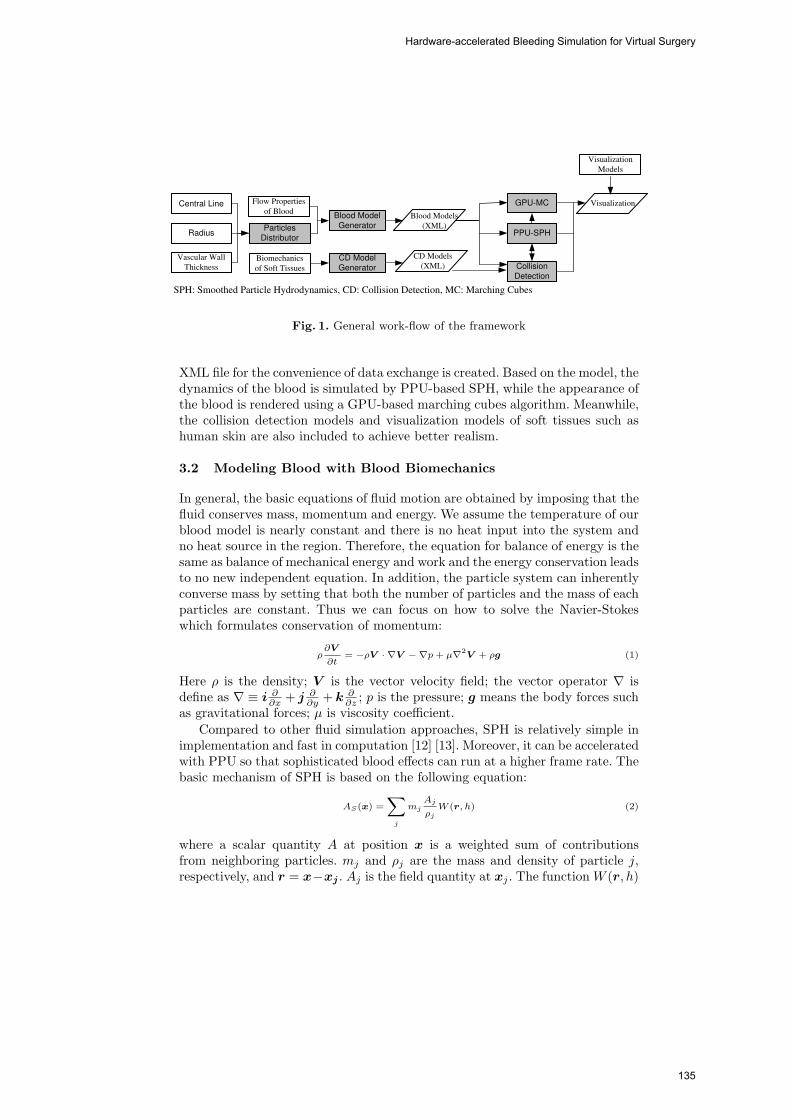
Central Line
Radius
Vascular Wall
Thickness
Particles
Distributor
Flow Properties
of BloodBlood Model
Generator
Biomechanics
of Soft Tissues
CD Model
Generator
Blood Models
(XML)
CD Models
(XML)
GPU-MC
PPU-SPH
Collision
Detection
Visualization
Visualization
Models
SPH: Smoothed Particle Hydrodynamics, CD: Collision Detection, MC: Marching Cubes
Fig. 1. General work-flow of the framework
XML file for the convenience of data exchange is created. Based on the model, thedynamics of the blood is simulated by PPU-based SPH, while the appearance ofthe blood is rendered using a GPU-based marching cubes algorithm. Meanwhile,the collision detection models and visualization models of soft tissues such ashuman skin are also included to achieve better realism.
3.2 Modeling Blood with Blood Biomechanics
In general, the basic equations of fluid motion are obtained by imposing that thefluid conserves mass, momentum and energy. We assume the temperature of ourblood model is nearly constant and there is no heat input into the system andno heat source in the region. Therefore, the equation for balance of energy is thesame as balance of mechanical energy and work and the energy conservation leadsto no new independent equation. In addition, the particle system can inherentlyconverse mass by setting that both the number of particles and the mass of eachparticles are constant. Thus we can focus on how to solve the Navier-Stokeswhich formulates conservation of momentum:
ρ∂V
∂t= −ρV · ∇V −∇p + μ∇2
V + ρg (1)
Here ρ is the density; V is the vector velocity field; the vector operator ∇ isdefine as ∇ ≡ i ∂
∂x + j ∂∂y + k ∂
∂z ; p is the pressure; g means the body forces suchas gravitational forces; μ is viscosity coefficient.
Compared to other fluid simulation approaches, SPH is relatively simple inimplementation and fast in computation [12] [13]. Moreover, it can be acceleratedwith PPU so that sophisticated blood effects can run at a higher frame rate. Thebasic mechanism of SPH is based on the following equation:
AS(x) =
∑j
mjAj
ρjW (r, h) (2)
where a scalar quantity A at position x is a weighted sum of contributionsfrom neighboring particles. mj and ρj are the mass and density of particle j,respectively, and r = x−xj . Aj is the field quantity at xj . The functionW (r, h)
Hardware-accelerated Bleeding Simulation for Virtual Surgery
135
is referred to as the smoothing kernel with the properties∫W (r, h)dr = 1 and
limh→0W (r, h) = δ(x), where h is the support radius and δ is the Dirac-function.Initially, particles have three quantities including mass, position and velocity.
In every time step of the simulation, SPH is used to evaluate the density (ρi) andthe force density (fpi , fvi ) caused by pressure and viscosity at particle i based onthe following equations derived in[14]:
ρi =∑j
mjW (r, h) (3)
fpi = −∇p(ri) = −
∑j
mj(pj + pi
2ρj)∇W (r, h) (4)
and
fvi = μ∇2
v(ra) = μ
∑j
mjV j − V i
ρj∇2
W (r, h) (5)
where r = xi−xj .Adding the gravitational force, we can get the total force den-sities. Thus based on Newton’s second law, we can compute acceleration, velocityand position of every particle. In the computation, we use built-in smoothingkernels (W (r, h)) in the PPU to ensure the stability of the simulation.
By centrifugation, the blood is separated into plasma and cells. The cellularcontents are essentially all erythrocytes or red cells. Normally, the red cells oc-cupy about 45%-50% of the blood volume[15]. To simplify the blood model, twokinds of particles are defined. One represents plasma and the other representsred cells. They are randomly distributed in the particle model in a pre-definedratio. Based on research of blood biomechanics, typical values of the density ofblood plasma and blood cells are 1025kg/m3 and 1125kg/m3 respectively, whilethe whole blood has a specific density between 1.056kg/m3 and 1.066kg/m3.More important, blood is a non-Newtonian fluid. In general, the constitutiveequation of an isotropic incompressible Newtonian fluid is:
γij = −pφij + 2μTij (6)
where
Tij =1
2(∂vi
∂xj+
∂vj
∂xi), (7)
Tii = T11 + T22 + T33 = 0. (8)
Here γij is the stress tensor, p is the hydrostatic pressure, φij is the isotropictensor or Kronecker delta, Tij is the strain-stress tensor, vi is the velocity com-ponent, and μ is a constant called the coefficient of viscosity. However, blooddoes not perform according to Equation (1) because the μ is not a constant.In our framework, we approximate the non-Newtonian behavior of blood bydynamically adjusting the value of viscosity in regular time steps. Some initialparameters such as the position and number of particles can be set based onCVH datasets.
3.3 Collision Detection between Blood and Soft Tissues
In PPU, Continuous Collision Detection(CCD) mechanism is provided for fastmoving objects, which is suitable for simulating interactions between blood and
Jing Qin, Wai-Man Pang, Yim-Pan Chui, Yong-Ming Xie, Tien-Tsin Wong, Wai-Sang Poon, Kwok Sui Leung, Pheng-Ann Heng
136
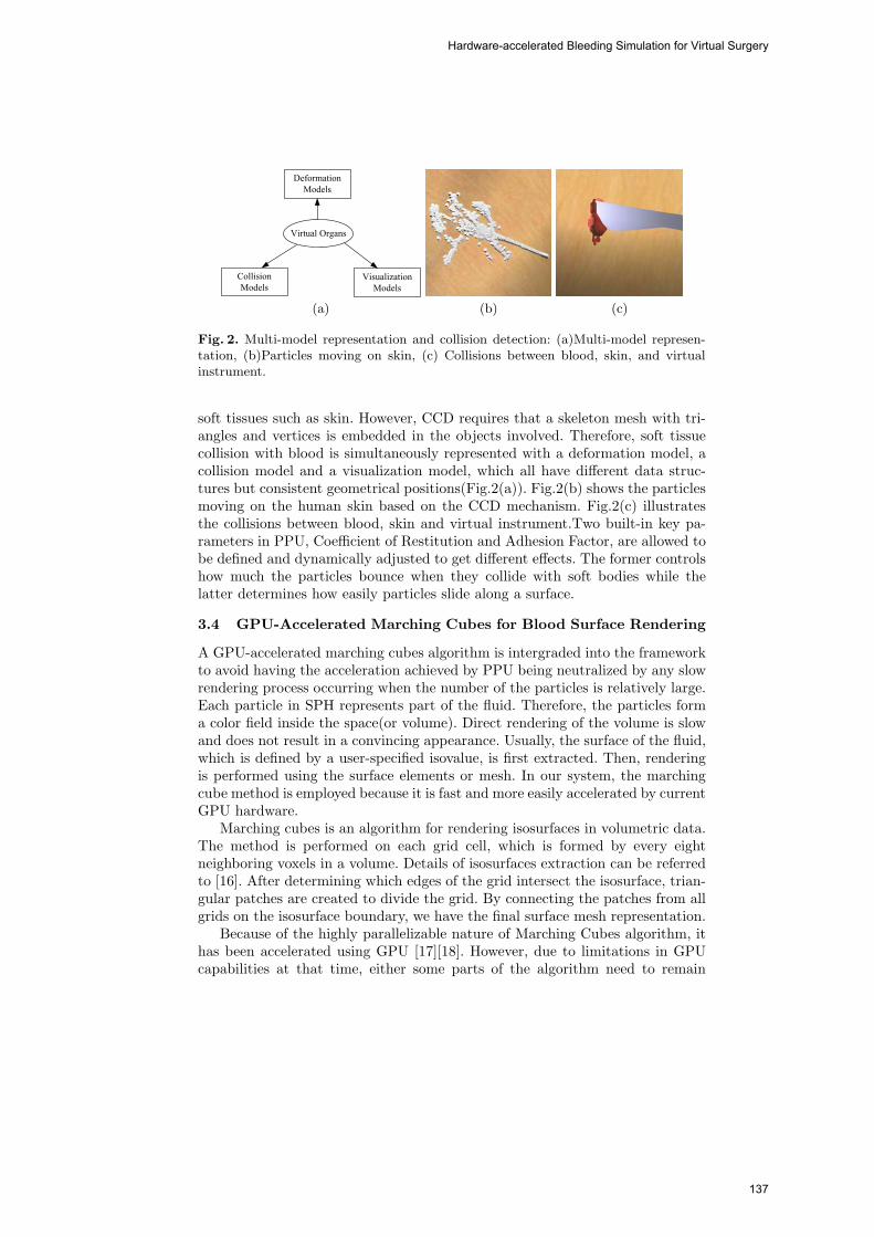
(a) (b) (c)
Fig. 2. Multi-model representation and collision detection: (a)Multi-model represen-tation, (b)Particles moving on skin, (c) Collisions between blood, skin, and virtualinstrument.
soft tissues such as skin. However, CCD requires that a skeleton mesh with tri-angles and vertices is embedded in the objects involved. Therefore, soft tissuecollision with blood is simultaneously represented with a deformation model, acollision model and a visualization model, which all have different data struc-tures but consistent geometrical positions(Fig.2(a)). Fig.2(b) shows the particlesmoving on the human skin based on the CCD mechanism. Fig.2(c) illustratesthe collisions between blood, skin and virtual instrument.Two built-in key pa-rameters in PPU, Coefficient of Restitution and Adhesion Factor, are allowed tobe defined and dynamically adjusted to get different effects. The former controlshow much the particles bounce when they collide with soft bodies while thelatter determines how easily particles slide along a surface.
3.4 GPU-Accelerated Marching Cubes for Blood Surface Rendering
A GPU-accelerated marching cubes algorithm is intergraded into the frameworkto avoid having the acceleration achieved by PPU being neutralized by any slowrendering process occurring when the number of the particles is relatively large.Each particle in SPH represents part of the fluid. Therefore, the particles forma color field inside the space(or volume). Direct rendering of the volume is slowand does not result in a convincing appearance. Usually, the surface of the fluid,which is defined by a user-specified isovalue, is first extracted. Then, renderingis performed using the surface elements or mesh. In our system, the marchingcube method is employed because it is fast and more easily accelerated by currentGPU hardware.
Marching cubes is an algorithm for rendering isosurfaces in volumetric data.The method is performed on each grid cell, which is formed by every eightneighboring voxels in a volume. Details of isosurfaces extraction can be referredto [16]. After determining which edges of the grid intersect the isosurface, trian-gular patches are created to divide the grid. By connecting the patches from allgrids on the isosurface boundary, we have the final surface mesh representation.
Because of the highly parallelizable nature of Marching Cubes algorithm, ithas been accelerated using GPU [17][18]. However, due to limitations in GPUcapabilities at that time, either some parts of the algorithm need to remain
Hardware-accelerated Bleeding Simulation for Virtual Surgery
137

running on CPU or several passes are required to complete the whole algorithm.Both scenarios introduce overheads and consequently degrade performance.
Fluid Volume
Geometry ShaderGrid cell
Fragment Shader
RenderingCell Indexing and Interpolation
Fig. 3. Blood rendering using GPU accelerated Marching Cube.
Utilizing the new Geometry Shader feature in the newest GPU supportingshader model 4.0, the marching cubes method can be performed entirely insidethe GPU in a single pass. Fig. 3. illustrates the whole process divided among dif-ferent shaders to complete the marching cubes implementation. First, marchingcubes grid cells are encoded as point primitives and sent to the geometry shader.The geometry shader operates on each point in parallel and generates a set oftriangles used to cut the cells according to the marching cubes code table. Next,the positions of constructed vertices are adjusted according to the voxel valuesin the grid cells. Finally, the isosurface is illuminated in the fragment shader fordisplay.
4 Experiment Results
4.1 Time Performance
The proposed framework has been implemented on a PC with the followingconfiguration: Pentium 4 Dual Core 3.2GHz CPU, 4GB RAM, NVIDIA GeForce8800 display adapter and AGEIA PhysXP1 physics processing unit. A series ofexperiments have been done to compare the time performance of CPU-basedbleeding simulation and our hardware-accelerated framework. Tables 1. and 2.show the experimental results. A significant speed improvement is observed whenPPU and GPU are used in bleeding simulation. The average frame rate of GPU-base MC is 29.7F/S at a volume size of 64×64×64, which can fulfill most real-time surgical simulation. The corresponding average frame rate of the CPU-based MC is only 5.6F/S. With the increase of the number of the particles, theadvantage of PPU-accelerated SPH is clearly revealed in Table 2. The framerate of PPU-based SPH stays above 50F/S while the CPU-based SPH is under10F/S when the number of particles is more than 5000. A dramatic decreaseof time performance of PPU-based SPH occurs when the number of particlesis more than 6000. This is maybe due to the PPU using relatively slow PCIbus interface to transfer data. Although this need to be verified through moreexperiments, in most cases, 6000 or fewer particles are enough to achieve realisticeffects.
Jing Qin, Wai-Man Pang, Yim-Pan Chui, Yong-Ming Xie, Tien-Tsin Wong, Wai-Sang Poon, Kwok Sui Leung, Pheng-Ann Heng
138

Table 1. The comparison between GPU and CPU-based MC for blood rendering
Volume Size Number of Triangles CPU(F/S) GPU(F/S)
32×32×32 15568 62.3 129.5
64×64×64 103822 5.6 29.7
128×128×128 967383 0.55 5.3
Table 2. The comparison between CPU and PPU-based SPH for bleeding simulation
Num. of Particles CPU(F/S) PPU(F/S) Num. of Particles CPU(F/S) PPU(F/S)
500 63.8 64.1 3000 16.4 55
1000 45.4 63.8 4000 12.3 53
1500 33.6 63.8 5000 9.3 49
2000 24.5 60 6000 7.1 7.1
2500 20.7 60 7000 6.2 6.3
4.2 Visualization
Fig. 4. shows the rendering results of our hardware-accelerated bleeding simula-tion. It demonstrates that our framework can simulate various bleeding phenom-ena with acceptable realism. The observed interaction between blood and skinvalidated the collision detection models. Fig. 5(a) and (b) show the bleedingeffects when integrating our framework to a virtual-reality based Orthopedicssurgery trainer (refer to attached video). Real-time and realistic bleeding simu-lation can help trainers learn how to handle various bleeding phenomena duringthe surgery and therefore improve their experience and skills.
5 Conclusion and Future Work
In this paper, a novel framework for real-time bleeding simulation with hardwareacceleration is presented. The relative computational advantage of the PhysicsProcessing Unit (PPU) is exploited for simulating bleeding based on SPH. Therealism is achieved by adjusting the biomechanical properties of the simulatedblood and providing proper collision detection between the simulated blood andsoft tissues. Furthermore, a GPU-based marching cubes algorithm is developedto accelerate the rendering process. Experimental results demonstrate that theframework achieves realistic and real-time simulation of bleeding. Future work in-cludes optimizing the marching cubes algorithm, integrating cutting algorithmsand haptic devices and developing simulators based on this bleeding simulationframework.
Acknowledgement The work described in this paper was supported in part byresearch grants from the Research Grants Council of the Hong Kong Special Ad-ministrative Region (Project No. CUHK 4223/04E and CUHK 4453/06M). Thiswork is affiliated with the Virtual Reality, Visualization and Imaging ResearchCenter at The Chinese University of Hong Kong as well as the Microsoft-CUHKJoint Laboratory for Human-Centric Computing and Interface Technologies.
Hardware-accelerated Bleeding Simulation for Virtual Surgery
139

(a) (b) (c)
(d) (e) (f)
Fig. 4. The visualization results of various bleeding phenomena with collision betweenblood and human skin: (a) trickling, (b) flowing, (c) pooling, (d) gushing, (e) pouring,and (f) dropping.
References
1. Ztonyi, J., Paget, R., Szkely, G., Bajka, M.: Real-time synthesis of bleeding forvirtual hysteroscopy. In: Proceedings of Medical Image Computing and Computer-Assisted Intervention MICCAI 2003. Volume 1. (November 2003) 67–74
2. Castro, M.A., Putman, C.M., Cebral, J.R.: Computational fluid dynamics model-ing of intracranial aneurysms:effects of parent artery segmentation on intraaneurys-mal hemodynamics. American Journal of Neuroradiology (27) (2006) 1703–1709
3. Bar-Joseph, Z., El-Yaniv, R., Lischinski, D., Werman, M.: Texture mixing and tex-ture movie synthesis using statistical learning. IEEE Transactions on Visualizationand Computer Graphics 7(2) (2001) 120–135
4. Quarteroni, A., Tuveri, M., Veneziani, A.: Computational vascular fluid dynamics:problems, models and methods. Computing and Visualization in Science 2(4)(2000) 163–197
5. Kurtcuoglu, V., Poulikalos, D.: Principles and challenges of computational fluiddynamics in medicine. In: 9th MICCAI Workshop on Computational BiomechanicsFor Medicine. (October 2006) 14–22
6. Svensson, J., Gardhagen, R., Heiberg, E., Ebbers, T., Loyd, D., Lanne, T., Karls-son, M.: Feasibility of patient specific aortic blood flow cfd simulation. In: Proceed-ings of Medical Image Computing and Computer-Assisted Intervention - MICCAI2006 Proceedings, Part I. (2006) 257–263
Jing Qin, Wai-Man Pang, Yim-Pan Chui, Yong-Ming Xie, Tien-Tsin Wong, Wai-Sang Poon, Kwok Sui Leung, Pheng-Ann Heng
140

(a) (b)
Fig. 5. Integrating our hardware-accelerated bleeding framework to a virtual-realitybased Orthopedics surgery trainer.(a)accidental cut at blood vessel (b)bleeding fromblood vessel.
7. Carlson, M., Mucha, P.J., R.B., V.H.I., Turk, G.: Melting and flowing. In: Pro-ceedings of the 2002 ACM SIGGRAPH Symposium on Computer Animation. (July2002) 167–174
8. Carlson, M., Mucha, P.J., Turk, G.: Rigid fluid: animating the interplay betweenrigid bodies and fluid. ACM Transaction on Graphics 23(3) (Aug 2004) 377–384
9. Stam, J., Fiume, E.: Depicting fire and other gaseous phenomena using diffusionprocesses. In: Computer Graphics Proceedings, Annual Conference Series, 1995(ACM SIGGRAPH ’95 Proceedings). (1995) 129–136
10. Muller, M., Schirm, S., Teschner, M.: Interactive blood simulation for virtualsurgery based on smoothed particle hydrodynamics. Journal of Technology andHealth Care 12(1) (2004) 25–31
11. Daenzer, S., Montgomery, K., Dillmann, R., Unterhinninghofen, R.: Real-timesmoke and bleeding simulation in virtual surgery. In: Proceedings of MedicineMeets Virtual Reality. (2007) 94–99
12. Libersky, L.D., Petschek, A.G., Carney, T.C., Hipp, J.R., Allahdadi, F.A.: Highstrain lagrangian hydrodynamics: a three-dimensional sph code for dynamic ma-terial response. Journal of Computational Physics 109 (1993) 67–75
13. Monaghan, J.J.: Simulating free surface flows with sph. Journal of ComputationalPhysics 110 (1994) 399–406
14. Muller, M., Charypar, D., Gross, M.: Particle-based fluid simulation for interactiveapplications. In: in Proceedings of ACM SIGGRAPH Symposium on ComputerAnimation (SCA). (2003) 154–159
15. Fung, Y.C.: Biomechanics: Mechanical Properties of Living Tissues. Second edn.Springer, Berlin Germany (1993)
16. Lorensen, W.E., Cline, H.E.: Marching cubes: A high resolution 3d surface con-struction algorithm. SIGGRAPH 87 Proceedings 21(4) (July 1987)
17. Goetz, F., Junklewitz, T., Domik, G.: Real-time marching cubes on the vertexshader. In: Eurographics 2005 Short Presentation. (2005)
18. Xie, Y., Heng, P.A., Wang, G., Wong, T.T.: Gpu-friendly marching cubes for visu-alizing translucent isosurfaces. In: Proceedings of Medicine Meets Virtual Reality.(2007) 500–503
Hardware-accelerated Bleeding Simulation for Virtual Surgery
141

Modeling Air-flow in the Tracheobronchial tree using Computational Fluid Dynamics
Ilhan Kaya1, Anand P. Santhanam2, Celina Imielinska3 and Jannick Rolland1,2
1 School of Computer Science and Engineering 2 CREOL, College of Optics and Photonics
University of Central Florida 4000 Central Florida Blvd Orlando, FL 32816
[email protected] Department of Biomedical Informatics, Columbia University,
701 West 168th Street New York, NY 10032
Abstract. In this paper, we present a biomechanical framework to model air-flow inside the bronchus and deformations across the tracheobronchial tree, pipeline for the simulator, theory and initial steps to realize this framework on a highly parallel graphical processing unit (GPU). We discuss the main chal-lenges expected and encountered to date. By using computational fluid dynam-ics (CFD) and computational solid dynamics (CSD) principles, we propose a numerical simulation framework that includes a biomechanical model of the tracheobronchial tree to simulate air flow inside the tree, on GPU in real-time. The proposed 3D biomechanical model to simulate the air inside the lungs cou-pled with a deformation model of the tracheobronchial tree, expressed through fluid-structure interaction, can be used to predict the transformations of the voxels from a 4D computed tomography (4DCT) dataset. Additionally, the pro-posed multi-functional CFD and CSD based framework is suitable for clinical applications such as adaptive lung radiotherapy, and a regional alveolar ventila-tion estimation.
1 Introduction
Lung cancer and various other ongoing or chronic lung diseases, e.g. closure of air-ways and emphysema, if lumped together, it is the number three killer in the United States. There has been a significant amount of research in analyzing the tissues of the lung through advanced imaging modalities such as Positron Emission Tomography (PET), Computerized Tomography (CT), and Magnetic Resonance Imaging (MRI). By applying various forms of medical image processing algorithms to CT, MRI, and PET images, anatomical structures and their material properties can be explored. Tawhai et al. make use of various forms of image segmentation algorithms to gener-ate subject-specific computational meshes of the human bronchial tree [1, 2]. Hoff-man et al. used deformable registration algorithms on CT scans to estimate the re-gional ventilation in ovine lungs [3, 4]. In the past few years, researchers all over the
142

world have been able to simulate natural phenomena such as fluids, gases, fire behav-ior on GPUs accurately and faster than CPUs. Three different approaches to simulate fluids in the field of computational fluid dynamics exist, fixed grid-based (Euler) or particle motion (Lagrange) and a hybrid Arbitrary Lagrangian-Eulerian (ALE). Eule-rian methods evaluate material properties at stationary grid points, whereas Lagran-gian methods employ moving grids with the material particles to solve the governing equations [5]. Kruger et al. built up a million Lagrangian particles to simulate and visualize 3D flow fields on non-uniform grids [6]. Dynamically regenerated meshes are used in [7] to simulate fluids. Viscoelastic material simulation based upon Eule-rian methods is shown in [8]. Harris et al. make use of GPU to simulate cloud dynam-ics whose state is governed by incompressible Navier Stokes (NS) equations [9, 10].
In this paper, we propose a simulation framework to simulate the air inside the tra-cheobronchial tree on GPU. As part of this framework, we propose a 3D biomechani-cal model which accounts for the air motion inside the tracheobronchial tree, and the deformations on the tracheobronchial tree. This work is the first of its kind to simulate elasticity theory and fluid dynamics to predict the displacements and deformations of the human tracheobronchial tree on GPU, which provides opportunity to run the simu-lation in real-time and on customer PCs. The framework and biomechanical model proposed might be used to account for the alveoli ventilation when it is combined with an image registration algorithm, and it can also account for transport of aerosol contained in cigarette smoking in human lung.
2 GPU Pipeline
GPUs are very powerful, highly parallel stream processing processors. Since they are specifically built for vector processing, they have a parallel computer architecture model. Their architecture is built upon single instruction multiple data (SIMD) para-digm. In SIMD, a single node dispatches the instruction to other processing nodes that compute the instruction with their own local data. SIMD computers provide superior-ity over instruction driven processors, CPUs, due to their parallel execution of the in-struction.
In Fig. 1 there is an illustration of floating point computational power of GPUs with respect to CPUs. This superiority makes GPUs an ideal platform to solve data-driven numerical problems in parallel. In a typical GPU, which is available on almost any PC sold today in market; there are one vertex and one fragment processor. Each processor is realized through several pipelines, working in parallel. In a NVIDIA GTX8800, which we use for our framework, there are 128 vertex and fragment proc-essors pipelines. In Fig. 2, the GPU pipeline that realizes the stream processing nature of these parallel machines is illustrated.
Modeling Air-flow in the Tracheobronchial tree using Computational Fluid Dynamics
143

Fig. 1. Illustration of 32-bit floating point GPU comparison courtesy of Engel et al [11].
Fig. 2. Graphical Processing Pipeline, GPU Architecture
3 Biomechanical Modeling of Air inside the Tracheobronchial Tree and its Deformations
The tracheobronchial tree geometry, shape, measurements and dimensions change for each individual. Average tracheal length ranges from 5.4 cm to 13.1 cm, as the age of the subjects changes from 2 to 20 [12]. Generally, air flow through the terminal bronchioles follows a laminar pattern, whereas air flow inside the trachea can be tur-bulent with high ventilation rates in abnormal conditions [13]. Hence our biome-chanical model consists of two parts to be able to correctly model the physics of the tracheobronchial tree: Modeling air inside the tracheobronchial tree, and modeling the deformations on the tracheobronchial tree.
3.1 Modeling air trough computational fluid dynamics (airway gas dynamics)
We model air inside the tracheobronchial tree as a fluid defined as any material which deforms continuously under shear stress. We make use of the continuum assumption of fluid mechanics, which states that fluid can be treated as an infinitely divisible sub-stance. We divide the solution domain into 3D infinitesimal cells, where the velocity and the density of the fluid are defined as average properties. Our modeling assump-tions for fluid is being incompressible, i.e. each cell has constant volume over time, homogeneous, density of the fluid stays constant in space, viscous, rate of deforma-
Ilhan Kaya, Anand P. Santhanam, Celina Imielinska and Jannick Rolland
144

tion is same under the same stress for all fluid cells. Fluid cells might experience de-formation, rotation, translation in space. The state of the fluid is determined through velocity of the each fluid cell, being a function of time and space, effectively repre-sented as a vector field, and pressure of each fluid cell, which is function of space and time.
3.1.1 Equations of Fluid State
Governing equations for fluid motion are the Navier-Stokes equations (NS). The state of the fluid, given by velocity and pressure, can be determined through solutions of NS.
(1)
(2)
In the above equations, u represents velocity, a vector quantity, having 3 compo-nents in 3D. If x(x,y,z) represents the position of the fluid cell, the velocity is u(x,t)and the pressure is p(x,t). ρ represents the density of the fluid, υ represents the kinematics viscosity. F(x,t) represent the external forces acting on the fluid including the gravitational force. The ( )uu ∇• term is called the advective term and it is the source of nonlinearity. It resembles the propagation of any disturbance caused by the
external forces acting on the fluid. The p∇ρ1 term is the effect of pressure on the
rate of change of the velocity. The u2∇υ term represents viscous diffusion. Due to viscosity, fluids are resistive to move, this resistance results in the distribution of momentum. Eq. 2 states the mass conversation since the fluid is assumed to be in-compressible. As for the boundary conditions to solve NS, we use no-slip velocity and pure Neumann pressure condition. No-slip velocity states that velocity is zero in all 3 dimensions at the boundaries. Pure-Neumann boundary conditions state that the rate of change of pressure is zero along the normal direction on the surface boundaries.
3.1.2 A Solution Method for Equations of Fluid State
The solution of NS, the set of Partial Differential Equations (PDE), can be found in many texts. We follow the lead of Griebel et al. [14] and Marsden et al. [15] Marsden et al. show the solution of the NS through a theorem in vector calculus. This theorem is called the Helmholtz-Hodge Decomposition Theorem. It states that in the same way a vector is decomposed into two components, a vector field can be decomposed into two vector fields. A divergent vector field w can be decomposed into a non-divergent vector field u and a vector field composed by the gradient of the scalar field. The Helmholtz Hodge decomposition theorem is shown in Eq. 3.
(3)
( ) Fuuuu +∇+∇−∇•−=∂∂ 21 υ
ρp
t0=•∇ u
p∇+= uw
Modeling Air-flow in the Tracheobronchial tree using Computational Fluid Dynamics
145

Since the application of external forces, advection and viscous diffusion, results in a divergent velocity field, w, at the end of each time step, we must satisfy the continu-ity requirement by subtracting the gradient of pressure field from the divergent veloc-ity field.
(4)
If we apply divergence to both sides of Eq 3, then we have p∇•∇+•∇=•∇ uw
p2∇=•∇ w (5)
Since u is a divergent-free vector field, u•∇ drops out. Eq. 5 is known as the Poisson-pressure equation. Once we have the pressure distribution, Eq. 4 gives the ve-locity at each time t, for any point in the fluid domain. We can further simplify Eq. 1 by defining a projection operator, �, which projects the divergent vector field w into its non-divergent vector field, u. If we apply � to both sides of Eq. 3,
( ) ( ) ( )p∇Ω+Ω=Ω uw (6)
By definition of �
(7)
If we substitute Eq. 7 into Eq. 6
(8)
Applying the projection operator � to Eq. 1 and substituting Eq. 8 into the resulting formulation will yield a drop out of the pressure term from Eq. 1.
(9)
3.2 Modeling tracheobronchial wall dynamics using linear elasticity theory
An important characteristic of the tracheobronchial tree is that it deforms constantly under shear stress due to its elastic nature. When the fluid starts to move inside the tracheobronchial tree, its pressure distribution causes displacements among other forces acting on the tracheobronchial tree. During an inhalation expiration cycle, changes in the transmural pressure inside and outside of the tracheobronchial tree causes deformations on the walls. These deformations furthermore change the boundaries for the fluid motion, resulting in displaced boundaries for the fluid simula-tion. This type of coupling between fluid and an elastic wall is modeled through Fluid-Structure Interaction (FSI). Fluid pressure distribution gives the force exerted upon the elastic wall, whereas elastic displacements calculated through elastic body theory of solid mechanics, give the new boundaries for fluid. Holzhauser et al. devel-oped a mathematical model to estimate the change in cross-sectional area of the tra-chea based upon a coupling between fluid flow and elastic theory [16]. FSI models
p∇−= wu
( ) ( ) uuw =Ω=Ω
( )p∇Ω=0
( )[ ]Fuuuu +∇+∇•−Ω=∂∂ 2υ
t
Ilhan Kaya, Anand P. Santhanam, Celina Imielinska and Jannick Rolland
146

are being also used in the simulation of blood flow in highly deformable arteries. In [17], authors developed a method to couple elastic arteries wall deformation as a moving boundary condition for blood flow. Equations for the incompressible fluid flow will be the same as given in Eq. 1. and Eq. 2. However the boundaries for the simulation for each time step will be redefined with the displacement calculated through the elasticity theory. Based on a staggered partition approach, we will divide the problem domain into two steps as shown by Griebel et al. [18]. At each time step, the fluid flow will be solved as if it has fixed boundaries, and the pressure distribution calculated by the fluid flow will be an input to the elasticity problem. Then newly cal-culated displacements through elasticity will be fed into fluid flow as new boundaries. Fig 3 gives an overview of FSI.
Fig. 3. A schematic of Fluid-Structure Interaction Modeling
In the elastic body deformation domain, time dependent Lame Equation serve as the mathematical formulation of the elasticity problem. It is given as
where u represents the displacement of elastic solid, Sρ is the density of elastic solid,
b are the external forces acting on the elastic solid, μ and λ are material specific Lame constants. It is to be noted that the b includes the force caused by the fluid flow. Finite methods have been extensively investigated for computing the solution of the elastic equation.
3.3 Biomechanical Model
Fig. 4. 2D cross-section of a 3D biomechanical model of the human tracheobronchial tree.
In Fig. 4, a 2D cross-section of our biomechanical model for the tracheobronchial tree is shown. This model utilizes a fluid flow model of CFD with an elasticity theory of CSD in a FSI. Inputs to this model is gravitational force, external forces acting on the tracheobronchial tree, volume-time curve of the subject inhalation exhalation cycle, computational geometry of tracheobronchial tree, inhaled air parameters, i.e viscosity,
buutu
SS ρμλμρ =•∇∇+−Δ−∂∂ )(2
2 (10)
Modeling Air-flow in the Tracheobronchial tree using Computational Fluid Dynamics
147
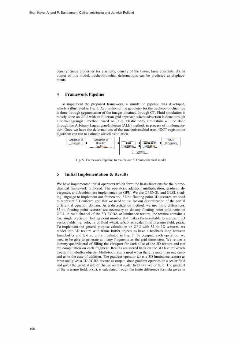
density, tissue properties for elasticity, density of the tissue, lame constants. As an output of this model, tracheobronchial deformations can be predicted as displace-ments.
4 Framework Pipeline
To implement the proposed framework, a simulation pipeline was developed, which is illustrated in Fig. 5. Acquisition of the geometry for the tracheobronchial tree is done through segmentation of the images obtained through CT. Fluid simulation is mostly done on GPU with an Eulerian grid approach where advection is done through a semi-Lagrangian method based on [19]. Elastic body simulation will be done through the Arbitrary Lagrangian-Eulerian (ALE) method, in process of implementa-tion. Once we have the deformations of the tracheobronchial tree, 4DCT registration algorithm can run to estimate alveoli ventilation.
Fig. 5. Framework Pipeline to realize our 3D biomechanical model
5 Initial Implementation & Results
We have implemented initial operators which form the basis functions for the biome-chanical framework proposed. The operators, addition, multiplication, gradient, di-vergence, and Jacobian are implemented on GPU. We use OPENGL and GLSL shad-ing language to implement our framework. 32-bit floating point 3D textures are used to represent 3D uniform grid that we need to use for our discretization of the partial differential equation domain. As a discretization method, we use finite differences. 32-bit floating point textures are necessary to do any floating point arithmetic on GPU. In each channel of the 3D RGBA or luminance texture, the texture contains a true single precision floating point number that makes them suitable to represent 3D vector fields, i.e. velocity of fluid w(x,t), u(x,t), or scalar fluid pressure field, p(x,t).To implement the general purpose calculation on GPU with 32-bit 3D textures, we render into 3D texture with frame buffer objects to have a feedback loop between framebuffer and texture units illustrated in Fig. 2. To compute each operation, we need to be able to generate as many fragments as the grid dimension. We render a dummy quadrilateral of filling the viewport for each slice of the 3D texture and run the computation on each fragment. Results are stored back on the 3D texture voxels trough framebuffer objects. Multi-texturing is used when there is more than one oper-and as in the case of addition. The gradient operator takes a 3D luminance texture as input and gives a 3D RGBA texture as output, since gradient operates on a scalar field and gives the greatest rate of change on that scalar field as a vector field. The gradient of the pressure field, p(x,t), is calculated trough the finite difference formula given in
Ilhan Kaya, Anand P. Santhanam, Celina Imielinska and Jannick Rolland
148

Eq. 11. We calculate the gradient of the pressure field to guarantee that the fluid obeys the divergent-free velocity assumption (incompressibility). Once the fluid is perturbed by an external force, the result is a divergent velocity field. This divergence on velocity field can be removed by subtracting the gradient of the pressure field at that time instant from the divergent velocity field according to the HelmHoltz Hodge theorem (Eq. 4).
(11)
The divergence operator takes a 3D velocity field, and gives a scalar field, so the input is a 3D RGBA texture, and the output is a luminance texture. Divergence of the velocity field is calculated trough the following finite difference formula.
(12)
For both the gradient and the divergence operators, we sample neighboring top, bottom, front, back, left, right voxels at a position in the grid in a GLSL shader and calculate the formulas presented with uniform grid dimension assumptions. Two Pois-son equations arise in the solution of fluid equations, the viscous diffusion and the Poisson pressure equations. Once the fluid has been perturbed by an external force, the result is a divergent velocity field. We can obtain the pressure distribution by solv-ing the Poisson pressure equation given in Eq. 5. In order to account for the viscosity of the fluid, we need to solve viscous diffusion equation, given in Eq. 13.
(13)
Poisson equations can be solved by many numerical iteration methods i.e conju-gate gradient, Gauss-Seidel, multi-grid, and Jacobian which are generally referred to as relaxation methods. We use the Jacobian due to its relatively easy implementation. By using the finite difference method, we expand the Laplacian operator, as it is given in Eq. 14.
(14)
Once we substitute Eq. 14 into Eq. 5, then we obtain the iteration equation for the Jacobi algorithm, which gives us the pressure distribution across the fluid.
(15)
We implemented these operators both on GPU and CPU, and plotted the frame per second (FPS) values versus the grid size as a comparison metric in Fig. 6. As it can be seen from Fig. 6, initially, when the grid dimension is small, CPU outperforms GPU, since it is designed to do general purpose computation, and setting up the fragment
( )zpp
ypp
xpp
zp
yp
xptp kjikjikjikjikjikji
δδδ 2,
2,
2,,, 1,,1,,,1,,1,,,1,,1 −+−+−+ −−−
��
���
�∂∂
∂∂
∂∂=∇ x
zww
yvv
xuu
zw
yv
xu kjikjikjikjikjikji
δδδ 2221,,1,,,1,,1,,,1,,1 −+−+−+ −
+−
+−
∂∂+
∂∂+
∂∂=•∇ u
ww 2∇=∂∂ υ
t
( ) 21,,,,1,,
2,1,,,,1,
2,,1,,,,1
2
2
2
2
2
22
)(2
)(2
)(2
,z
pppy
pppx
pppzp
yp
xptp kjikjikjikjikjikjikjikjikji
δδδ−+−+−+ +−
++−
++−
��
���
�∂∂+
∂∂+
∂∂=∇ x
6)( 2
1,,1,,,1,,1,,,1,,11,,
w•∇∂−+++++= −+−+−++ xpppppp
pn
kjin
kjin
kjin
kjin
kjin
kjinkji
Modeling Air-flow in the Tracheobronchial tree using Computational Fluid Dynamics
149

pipeline on GPU takes up time. Once the grid dimension becomes 32 or higher, GPU outperforms CPU 10-30 times, being similar to the plot given in Fig. 1.
GPU vs CPU speedup
0
2000
4000
6000
8000
10000
12000
16 32 64 128 256
3D Grid Size
FPS
GPUdivergenceCPUdivergenceGPUgradientCPUgradientGPUmultiplyCPUmultiplyGPUaddCPUadd
Fig. 6. GPU vs. CPU FPS comparison of the framework operators
6 Challenges
Poulikakos et al. have shown general challenges encountered while applying CFD methods to simulate fluids inside the human body, i.e. blood, cerebrospinal fluid [20]. In a similar way, we now list the challenges in implementing our biomechanical model. The complex geometry of the tracheobronchial tree makes the image acquisi-tion and processing steps tedious. Due to the coupling of the elasticity problem with the fluid flow, fluid boundaries are modified at each time step, so traction of the boundaries is required. Hence boundary conditions are the Achilles’s hill of the prob-lem. As for the elasticity problem, material properties i.e. lame constants, density of tracheobronchial wall tissue, need to be specified. For the external forces acting on the exterior of the elastic tracheobronchial tree, an inverse computational dynamics approach needs to be specified. Numerical simulation of the problem requires discre-tization. For the fluid flow we use a finite-difference scheme. This is simple yet not suitable for fluid-structure problem. In order to solve Poisson Equations, Jacobi’s it-eration is used. Convergence and stability of numerical methods used in implementa-tion should be verified.
7 Conclusion
In this paper we present a biomechanical framework to simulate air motion inside the tracheo-bronchial tree and estimate the deformations of the tracheobronchial tree caused by this fluid flow. This framework is being realized on GPU. The biomechani-cal model combines a fluid flow model based upon CFD with an elastic model of CSD. Furthermore, a simulator pipeline is given in this paper. Initial implementation results have been shown and challenges discussed.
Acknowledgements. This work is supported by US Army Medical Research and Ma-terial Command.
Ilhan Kaya, Anand P. Santhanam, Celina Imielinska and Jannick Rolland
150
References
[1] Tawhai M. H., Hunter P.,Tschirren J., Reinhardt J.,McLennan G., Hoffman E.A.:CT-based Geometry Analysis and Finite Element Models of the Human and Ovine Broncial Tree. J. Appl. Physiol. Vol. 97 (2004) 2310-2321.
[2] Tawhai M. H., Pullan A.J., Hunter P.J.: Generation of an Anatomically-Based Three Di-mensional Model of the Conducting Airways. Annals of Biomechanical Engineering. Vol 28 (2000) 793-802.
[3] Pan Y., Kumar D., Hoffman E.A., Christensen G.E., McLennan G., Song H.J., Ross A., Simon B.A., Reinhardt J.: Estimation of Regional Lung Expansion via 3D image Registra-tion. Proceedings of SPIE Vol. 5746. Bellingham, USA (2005).
[4] Tawhai M. H., Nash M.P., Hoffman E.A.:A Imaging Based Computational Approach to Model Ventilation Distribution and Soft-tissue Deformation in the Ovine Lung. Academic Radiology. Vol. 13 (2006) 113-120.
[5] Feldman B.E., O’Brian J.F., Klingner B.M.,Goktekin G.E.: Fluids in Deforming Meshes. Proceedings of 2005 ACM SIGGRAPH/Eurographics Symposium. on Computer Animation. Los Angeles, USA (2005).
[6] Kruger J., Kipfer P., Kondratieva P.,Westermann R.: A particle System for Interactive Visu-alization of 3D Flows. IEEE T. on Visualization and Computer Graphics. Vol. 11 (2005) 744-756.
[7] Klingner B.M., Feldman B.E., Nuttapong C., O’Brian J.F.: Fluid Animation with Dynamic Meshes. Proceedings of 2006 ACM SIGGRAPH. Boston, USA (2006).
[8] Goktekin G. T., Barteil W. A., O’Brain J.F.: A Method for Animating Viscoelastic Fluids. Proceedings of 2004 ACM SIGGRAPH. Los Angeles, USA (2004).
[9] Harris J. M., Baxter V. W., Scheuermann T.,Lastra A.: Simulation of Cloud Dynamics on Graphics Hardware. Proceedings of 2003 ACM SIGGRAPH / Eurographics Conference on Graphics Hardware. San Diego, USA (2003).
[10] Harris J.M.: Fast Fluid Dynamics Simulation on the GPU. In GPU Gems Programming Techniques, Tips, Tricks for Real-time Graphics, Fernondo R. (Ed) Addison-Wesley Profes-sional Boston (2004) 637-665.
[11] Engel K., Hadwiger M., Kniss M.J., Rezk-Salama C., Weiskopf D.:Real-Time Volume Graphics. A. K. Peters Ltd, Wellesley, USA (2006).
[12] Griscom N.T., and Wohl M.E.: Dimensions of the Growing Trachea Related to Age and Gender. American Journal of Roentgenology. Vol 146 (1986) 233-237.
[13] West J.B.: Respiratory Physiology- The Essentials (7th Ed). Lippincott Williams & Wilkins (2005).
[14] Griebal M., Dornseifer T., NeunHoeffer T.: Numerical Simulation in Fluid Dynamics- A practical Introduction. Society for Industrial and Applied Mathematics (SIAM), Philadel-phia, USA (1998).
[15] Chorin A.J., and Marsden J.E.: A Mathematical Introduction to Fluid Mechanics (4th Ed). Springer, (2000)
[16] Holzhauser U. and Lambert R.K.: Analysis of Tracheal Mechanics and Applications. J. Appl. Physiol. Vol. 91 (2006) 290-297.
[17] Figueroa A., Vignon-Clementel I., Jansen K.E., Hughes J.R.T., Taylor C.A.: A Coupled Momentum Method for Modeling Blood Flow in Three-Dimensional Deformable Arteries. Computer Methods in Applied Mechanics and Engineering. Vol. 195 (2006) 5685-5706
[18] Engel M., and Griebel M.: Flow Simulation on Moving Boundary-fitted Grids and Appli-cation to Fluid-Structure Interaction Problems. Int. J. Numerical Meth. In Fluids. Vol. 50 (2006) 437-468
[19] Stam J.:Stable Fluids. Proceedings of 1999 ACM SIGGRAPH. Los Angeles, USA (1999). [20] Paulikakos D., Kurtcuoglu V.: Principles and Challenges of Computational Fluid Dynam-
ics in Medicine. In 9th International MICCAI Conference, Copenhagen, Denmark (2006).
Modeling Air-flow in the Tracheobronchial tree using Computational Fluid Dynamics
151

Imaging Facial Signs of Neuro-PhysiologicalResponses
Dvijesh Shastri1, Arcangelo Merla2, Panagiotis Tsiamyrtzis3, Ioannis Pavlidis1�
Computational Physiology Lab1,Department of Computer Science,
University of Houston, Houston, TX, USA,[email protected],[email protected]
ITAB - Institute of Advanced Biomedical Technologies2,Department of Clinical Sciences and Bioimaging,
University “G. D’Annunzio”,Chieti, Italy
Department of Statistics3,Athens University of Economics and Business
Athens, [email protected]
Abstract. In the present paper, we introduce an integrated frameworkfor detecting peripheral sympathetic responses through purely imagingmeans. The measurements are performed on three facial areas of sym-pathetic importance, that is, periorbital, supraorbital, and maxillary. Tothe best of our knowledge, this is the first time that the sympatheticimportance of the maxillary area is analyzed. Because the imaging mea-surements are thermal in nature and are composed of multiple compo-nents of variable frequency (i.e., blood flow, sweat gland activation, andbreathing), we chose wavelets as the image analysis framework. The im-age analysis is grounded on GSR signals, which are still considered thegolden standard in peripheral neurophysiological and psychophysiologi-cal studies. The experimental results show that monitoring of the facialchannels yields similar detecting power to GSR’s.
1 Introduction
The Autonomic Nervous System (ANS) and particularly its sympathetic divisionhas been the object of intense study in neurophysiology and psychophysiology.The sympathetic division readies the body for a crisis that may require sudden,intense physical activity. It is a primal survival mechanism. Therefore, intereston methodologies that scrutinize sympathetic responses is well founded and hasmany applications.
� To whom all correspondence should be addressed
152
2
When sympathetic activation occurs, an individual experiences increased ac-tivity in the cardiovascular and respiratory centers of the pons and medulla ob-longata, leading to elevations in blood pressure, heart rate, breathing rate, anddepth of respiration. These vital sign changes are mediated through adrener-gic postganglionic fibers. Determination of sympathetic activation through vitalsign monitoring is not always straightforward.
As an alternative, researchers focused their efforts on sympathetic manifes-tations effected through cholinergic postganglionic fibers. These fibers innervatesweat glands of the skin and the blood vessels to skeletal muscles and the brain.They provide a pathway to stimulating sweat gland secretion and selectivelyenhancing blood flow to muscles.
In this context, Electro-Dermal Activity (EDA) has been the gold standardfor peripheral monitoring of sympathetic responses. EDA is measured throughthe Galvanic Skin Response (GSR), which is a simple and reproducible methodfor quantifying sweat gland activation in the palm. Alternatively, EDA can becaptured through a palm thermistor, which registers the full thermoregulatoryphenomenon including changes both in blood flow and sweat gland activation.In our case, this is a useful yardstick, as it provides palm information similar tothe one thermal imaging provides for the face.
Indeed, in recent years, we have demonstrated that during arousal addi-tional physiological signs materialize on the face. Specifically, we have shownthat increased blood flow in the periorbital [1][2] and supraorbital [3] areas areubiquitous manifestations of stress. We have also developed a thermal imagingmethodology to extract both the periorbital and supraorbital signals.
In the present paper, we link traditional probe-based with the newer image-based neurophysiological methodologies. We study comparatively the periorbital,supraorbital, and palm channels (GSR and thermistor) within a classic repeatedarousal experiment. First, we introduce a novel modeling methodology to quan-tify the GSR signal and validate the arousal experiment. In addition, we demon-strate that concomitantly to the palm area, strong sweat gland activation ismanifested in the maxillary area. This is one more sympathetic thermoregula-tory phenomenon manifested on the face. Therefore, it can be sensed and com-puted through thermal imaging. We apply a wavelets analysis method for allchannels (periorbital, supraorbital, maxillary, GSR, and palm thermistor). Theresults reveal tonic (baseline) and phasic (event related) affinity of the threeimaging channels to the GSR and palm thermistor channels. We also identifythe presence of a breathing component in the maxillary signal.
Our research brings to the fore the pivotal role of facial physiology in themanifestation of stress and establishes the methodological framework for sensingperipheral sympathetic responses through imaging means.
In the rest of the paper we unveil our new imaging methodology for model-ing and analyzing the facial sympathetic channels. Specifically, in section 2, wedescribe the method itself. In section 3, we report and discuss its experimentalvalidation.
Imaging Facial Signs of Neuro-Physiological Responses
153
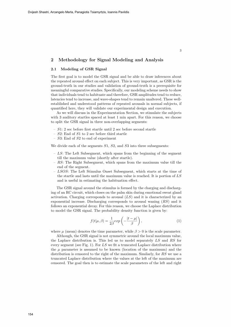
3
2 Methodology for Signal Modeling and Analysis
2.1 Modeling of GSR Signal
The first goal is to model the GSR signal and be able to draw inferences aboutthe repeated arousal effect on each subject. This is very important, as GSR is theground-truth in our studies and validation of ground-truth is a prerequisite formeaningful comparative studies. Specifically, our modeling scheme needs to showthat individuals tend to habituate and therefore, GSR amplitudes tend to reduce,latencies tend to increase, and wave-shapes tend to remain unaltered. These well-established and understood patterns of repeated arousals in normal subjects, ifquantified here, they will validate our experimental design and execution.
As we will discuss in the Experimentation Section, we stimulate the subjectswith 3 auditory startles spaced at least 1 min apart. For this reason, we chooseto split the GSR signal in three non-overlapping segments:
– S1: 2 sec before first startle until 2 sec before second startle– S2: End of S1 to 2 sec before third startle– S3: End of S2 to end of experiment
We divide each of the segments S1, S2, and S3 into three subsegments:
– LS: The Left Subsegment, which spans from the beginning of the segmenttill the maximum value (shortly after startle).
– RS: The Right Subsegment, which spans from the maximum value till theend of the segment.
– LSOS: The Left Stimulus Onset Subsegment, which starts at the time ofthe startle and lasts until the maximum value is reached. It is portion of LSand is useful in estimating the habituation effect.
The GSR signal around the stimulus is formed by the charging and discharg-ing of an RC circuit, which closes on the palm skin during emotional sweat glandactivation. Charging corresponds to arousal (LS) and it is characterized by anexponential increase. Discharging corresponds to arousal waning (RS) and itfollows an exponential decay. For this reason, we choose the Laplace distributionto model the GSR signal. The probability density function is given by:
f(t|μ, β) =12βexp
(−|t− μ|
β
), (1)
where μ (mean) denotes the time parameter, while β > 0 is the scale parameter.Although, the GSR signal is not symmetric around the local maximum value,
the Laplace distribution is. This led us to model separately LS and RS forevery segment (see Fig. 1). For LS we fit a truncated Laplace distribution wherethe μ parameter is assumed to be known (location of the maximum) and thedistribution is censored to the right of the maximum. Similarly, for RS we use atruncated Laplace distribution where the values at the left of the maximum arecensored. The goal then is to estimate the scale parameters of the left and right
Dvijesh Shastri, Arcangelo Merla, Panagiotis Tsiamyrtzis, Ioannis Pavlidis
154

4
Fig. 1. GSR segments S1, S2, and S3 along with the fitted Laplace values for subjectSub1. The stimuli occurrences have been marked appropriately.
distributions (i.e., βL and βR). This estimation is done through the OrdinaryLeast Squares (OLS) method.
For LS where t ≤ μ, we have:
y = f(t) =1
2βLexp
(−μ− tβL
)⇒ ln(y) =
[− μ
βL− ln(2βL)
]+
1βLt, (2)
so that time t and logarithmic scale ln(y) are linearly related. We use OLS toestimate the slope, whose inverse is the parameter of interest βL.
For RS where t ≥ μ, we have:
y = f(t) =1
2βRexp
(− t− μβR
)⇒ ln(y) =
[μ
βR− ln(2βR)
]− 1βRt, (3)
so that time t and logarithmic scale ln(y) are linearly related. We use OLS toestimate the slope, whose negative inverse is the parameter of interest βR.
For LSOS we apply linear (versus exponential) fitting, as these subsegmentsare nearly impulsive.
2.2 Wavelets Analysis of Sympathetic Signals
We extract thermal signals from three facial areas: periorbital, supraorbital, andmaxillary. In all three cases the regions of interest are tracked using the coali-tional tracking method we reported in [4]. In the periorbital area, the extractedsignal is formed from the evolution of the mean thermal footprint of the facialarteriovenous complex. This footprint is segmented via a fuzzy segmentation al-gorithm, which is seeded in the initial frame with two points in the inner orbitalareas (see Fig. 2). On each subsequent frame, the seeds are adjusted with helpfrom the coalitional tracker. In the supraorbital area, the extracted signal isformed from the evolution of the mean thermal footprint of the entire region ofinterest. In the maxillary area, the extracted signal is formed from the evolutionof the mean thermal footprint of the entire region of interest.
The periorbital thermal signal is a correlate of the blood supply to the orbitalmuscle. The supraorbital thermal signal is a correlate of the blood supply to
Imaging Facial Signs of Neuro-Physiological Responses
155
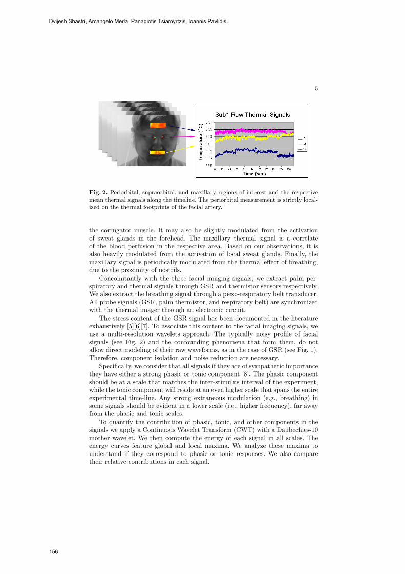
5
Fig. 2. Periorbital, supraorbital, and maxillary regions of interest and the respectivemean thermal signals along the timeline. The periorbital measurement is strictly local-ized on the thermal footprints of the facial artery.
the corrugator muscle. It may also be slightly modulated from the activationof sweat glands in the forehead. The maxillary thermal signal is a correlateof the blood perfusion in the respective area. Based on our observations, it isalso heavily modulated from the activation of local sweat glands. Finally, themaxillary signal is periodically modulated from the thermal effect of breathing,due to the proximity of nostrils.
Concomitantly with the three facial imaging signals, we extract palm per-spiratory and thermal signals through GSR and thermistor sensors respectively.We also extract the breathing signal through a piezo-respiratory belt transducer.All probe signals (GSR, palm thermistor, and respiratory belt) are synchronizedwith the thermal imager through an electronic circuit.
The stress content of the GSR signal has been documented in the literatureexhaustively [5][6][7]. To associate this content to the facial imaging signals, weuse a multi-resolution wavelets approach. The typically noisy profile of facialsignals (see Fig. 2) and the confounding phenomena that form them, do notallow direct modeling of their raw waveforms, as in the case of GSR (see Fig. 1).Therefore, component isolation and noise reduction are necessary.
Specifically, we consider that all signals if they are of sympathetic importancethey have either a strong phasic or tonic component [8]. The phasic componentshould be at a scale that matches the inter-stimulus interval of the experiment,while the tonic component will reside at an even higher scale that spans the entireexperimental time-line. Any strong extraneous modulation (e.g., breathing) insome signals should be evident in a lower scale (i.e., higher frequency), far awayfrom the phasic and tonic scales.
To quantify the contribution of phasic, tonic, and other components in thesignals we apply a Continuous Wavelet Transform (CWT) with a Daubechies-10mother wavelet. We then compute the energy of each signal in all scales. Theenergy curves feature global and local maxima. We analyze these maxima tounderstand if they correspond to phasic or tonic responses. We also comparetheir relative contributions in each signal.
Dvijesh Shastri, Arcangelo Merla, Panagiotis Tsiamyrtzis, Ioannis Pavlidis
156
6
3 Experimentation and Discussion
We used a high quality Thermal Imaging (TI) system for data collection. Thecenterpiece of the TI system is a ThermoVision SC6000 Mid-Wave Infrared(MWIR) camera [9] (NEDT=0.025◦C). We recorded 10 thermal clips from thefaces of 10 subjects while resting in an armchair. Concomitantly, we recordedground-truth GSR, palm thermistor, and piezo-respiratory signals with the Pow-erLab 8/30, ML870 data acquisition system [10]. The data set features subjectsof both genders, different races, and with varying physical characteristics. Thesubjects were focused on a mental task while they were measured through thethermal imaging and contact sensors. The experiment lasted 4 min. After thefirst minute the first auditory startle was delivered and after that two more weredelivered spaced at least 1 min apart. The experiment ended about 1 min afterthe delivery of the third startle.
3.1 GSR Results
We applied the modeling methodology detailed in Section 2.1 to each segmentof every GSR waveform. Therefore, we had 3 segments (S1, S2, S3) × 3 sub-segments (LS, RS, LSOS) × 10 subjects = 90 cases for which we needed toestimate the scale parameter β (Laplace fitting for LS and RS) or the slope (lin-ear fitting for LSOS). The results are shown in Table 1 and elicit the followingconclusions:
– For all stimuli (S1, S2 and S3) LS has a much smaller scale parameter thanRS indicating that the phenomenon causes a steep increase and then decaysat a much lower rate.
– Comparing the LS parts of S1, S2, and S3, within the same subject, weobserve that usually the 1st stimulus causes the steepest increase and as wemove to subsequent stimuli the response is less steep (i.e., the βL parameteris increasing).
– Comparing the RS parts of S1, S2, and S3, within the same subject, weobserve that usually the subject recovers slowly after the 1st stimulus (i.e.,it has a high βR parameter). Recovery from subsequent stimuli is becomingfaster (smaller βR parameter).
– Comparing the LSOS parts of S1, S2, and S3, within the same subject,we observe that the estimated (positive) slope of the linear regression isdecreasing as we move from S1 to S2 to S3 (habituation).
These conclusions are in accordance with the expected behavior of normal sub-jects, and therefore our experiment is valid.
3.2 Comparative Wavelets Analysis Results
We applied the wavelets analysis methodology detailed in Section 2.2 for all 6sympathetic signals from all 10 subjects. Fig. 3 shows the wavelet energy curves
Imaging Facial Signs of Neuro-Physiological Responses
157
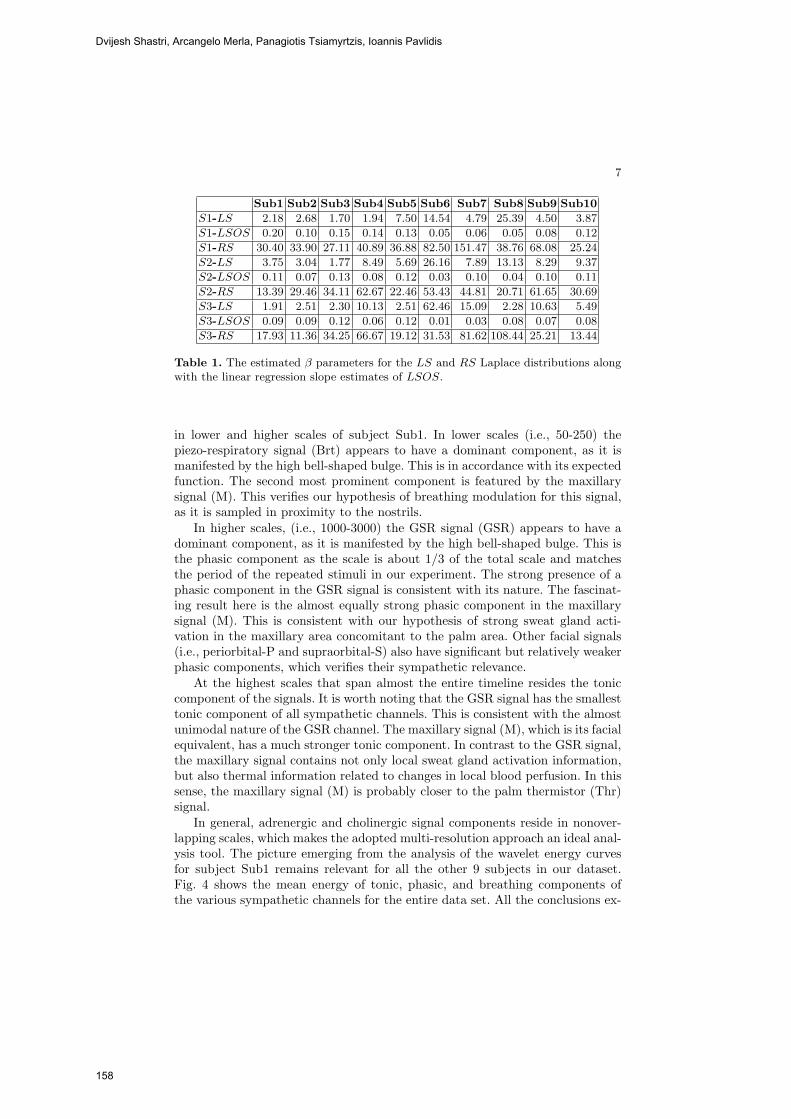
7
Sub1 Sub2 Sub3 Sub4 Sub5 Sub6 Sub7 Sub8 Sub9 Sub10
S1-LS 2.18 2.68 1.70 1.94 7.50 14.54 4.79 25.39 4.50 3.87
S1-LSOS 0.20 0.10 0.15 0.14 0.13 0.05 0.06 0.05 0.08 0.12
S1-RS 30.40 33.90 27.11 40.89 36.88 82.50 151.47 38.76 68.08 25.24
S2-LS 3.75 3.04 1.77 8.49 5.69 26.16 7.89 13.13 8.29 9.37
S2-LSOS 0.11 0.07 0.13 0.08 0.12 0.03 0.10 0.04 0.10 0.11
S2-RS 13.39 29.46 34.11 62.67 22.46 53.43 44.81 20.71 61.65 30.69
S3-LS 1.91 2.51 2.30 10.13 2.51 62.46 15.09 2.28 10.63 5.49
S3-LSOS 0.09 0.09 0.12 0.06 0.12 0.01 0.03 0.08 0.07 0.08
S3-RS 17.93 11.36 34.25 66.67 19.12 31.53 81.62 108.44 25.21 13.44
Table 1. The estimated β parameters for the LS and RS Laplace distributions alongwith the linear regression slope estimates of LSOS.
in lower and higher scales of subject Sub1. In lower scales (i.e., 50-250) thepiezo-respiratory signal (Brt) appears to have a dominant component, as it ismanifested by the high bell-shaped bulge. This is in accordance with its expectedfunction. The second most prominent component is featured by the maxillarysignal (M). This verifies our hypothesis of breathing modulation for this signal,as it is sampled in proximity to the nostrils.
In higher scales, (i.e., 1000-3000) the GSR signal (GSR) appears to have adominant component, as it is manifested by the high bell-shaped bulge. This isthe phasic component as the scale is about 1/3 of the total scale and matchesthe period of the repeated stimuli in our experiment. The strong presence of aphasic component in the GSR signal is consistent with its nature. The fascinat-ing result here is the almost equally strong phasic component in the maxillarysignal (M). This is consistent with our hypothesis of strong sweat gland acti-vation in the maxillary area concomitant to the palm area. Other facial signals(i.e., periorbital-P and supraorbital-S) also have significant but relatively weakerphasic components, which verifies their sympathetic relevance.
At the highest scales that span almost the entire timeline resides the toniccomponent of the signals. It is worth noting that the GSR signal has the smallesttonic component of all sympathetic channels. This is consistent with the almostunimodal nature of the GSR channel. The maxillary signal (M), which is its facialequivalent, has a much stronger tonic component. In contrast to the GSR signal,the maxillary signal contains not only local sweat gland activation information,but also thermal information related to changes in local blood perfusion. In thissense, the maxillary signal (M) is probably closer to the palm thermistor (Thr)signal.
In general, adrenergic and cholinergic signal components reside in nonover-lapping scales, which makes the adopted multi-resolution approach an ideal anal-ysis tool. The picture emerging from the analysis of the wavelet energy curvesfor subject Sub1 remains relevant for all the other 9 subjects in our dataset.Fig. 4 shows the mean energy of tonic, phasic, and breathing components ofthe various sympathetic channels for the entire data set. All the conclusions ex-
Dvijesh Shastri, Arcangelo Merla, Panagiotis Tsiamyrtzis, Ioannis Pavlidis
158

8
(a) (b)
Fig. 3. Wavelet energy curves of subject Sub1 for all 6 sympathetic channels in (a)lower and (b) higher scales.
tracted through the example of subject Sub1 still apply for the thus statisticallyconstructed mean subject.
Fig. 4. Mean tonic, phasic, and breathing energy components for the various sympa-thetic channels.
References
[1] Levine, J., Pavlidis, I., Cooper, M.: The face of fear. The Lancet 357(9270) (2001)1757
[2] Pavlidis, I., Eberhardt, N., Levine, J.: Human behavior: Seeing through the faceof deception. Nature 415(6867) (2002) 35
[3] Puri, C., Olson, L., Pavlidis, I., Starren, J.: Stresscam: Non-contact measurementof users’ emotional states through thermal imaging. In: Proceedings of the 2005ACM Conference on Human Factors in Computing Systems (CHI), Portland,Oregon (2005) 1725–8
[4] Dowdall, J., Pavlidis, I., Tsiamyrtzis, P.: Coalitional tracking. Computer Visionand Image Understanding (2007)
Imaging Facial Signs of Neuro-Physiological Responses
159

9
[5] Baba, M., Watahiki, Y., Matsunaga, M., Takebe, K.: Sympathetic skin responsein healthy man. Electromyography Clinincal Neurophysiology 28 (1988) 277–283
[6] Uncini, A., Pullman, S., Lovelace, R., Gambi, D.: The sympathetic skin response:Normal values, elucidation of afferent components and application limits. TheJournal of Neuroscience 87 (1988) 299–306
[7] Elie, B., Guiheneuc, P.: Sympathetic skin response: Normal results in differ-ent experimental conditions. Electroencephalogry and Clinical Neurophysiology76(258-267) (1990)
[8] Lim, C., Renniea, C., Barry, R., Bahramali, H., Lazzaro, I., Manor, B., Gordon, E.:Decomposing skin conductance into tonic and phasic components. InternationalJournal of Psychophysiology 25 (1997) 97–109
[9] FLIR Systems 70 Castilian Dr., Goleta, California 93117: (http://www.flir.com)[10] ADInstruments 2205 Executive Circle, Colorado Springs, Colorado 80906:
(http://www.adinstruments.com)
Dvijesh Shastri, Arcangelo Merla, Panagiotis Tsiamyrtzis, Ioannis Pavlidis
160

A novel partnership between surgeons and machines, made possible by advances in computing and engineering technology, could overcome many of the limitations of traditional surgery. By extending the surgeons' ability to plan and carry out surgical interventions more accurately and with less trauma, Computer-Integrated Surgery (CIS) systems could help to improve clinical outcomes and the efficiency of health care delivery. CIS systems could have a similar impact on surgery to that long since realized in Computer-Integrated Manufacturing (CIM). Mathematical modeling and computer simulation have proved tremendously successful in engineering. Computational mechanics has enabled technological developments in virtually every area of our lives. One of the greatest challenges for mechanists is to extend the success of computational mechanics to fields outside traditional engineering, in particular to biology, biomedical sciences, and medicine. The workshop provided an opportunity for computational biomechanics specialists to present and exchange opinions on the opportunities of applying their techniques to computer-integrated medicine.