THE ROLE OF EMPLOYMENT EXPERIENCE IN

EXPLAINING THE GENDER WAGE GAP

Michal MyckGillian Paull

THE INSTITUTE FOR FISCAL STUDIES

WP04/16

THE ROLE OF EMPLOYMENT EXPERIENCE IN EXPLAINING

THE GENDER WAGE GAP

Michal Myck and Gillian Paull

Institute for Fiscal Studies

July 2004

JEL Classification: J16, J41, C23. Keywords: gender wage gap, returns to experience, artificial panel data.

ACKNOWLEDGEMENTS We gratefully acknowledge the support of the Leverhulme Trust under the project “The Changing Distribution of Consumption, Economic Resources and the Welfare of Households”. We are also grateful for comments from seminar participants at the IFS and from conference participants at the Spring Meeting of Young Economists in Copenhagen in 2001 and at the AEA “Econometrics of Wages” Conference in Brussels in May 2002. Corresponding Author: Gillian Paull, Institute of Fiscal Studies, 7 Ridgmount Street, London WC1E 7AE, tel: 020-8241-2895, e-mail: gill_p@ifs.org.uk

EXECUTIVE SUMMARY

The wage gap between male and female workers has narrowed in both the US and

the UK over the past twenty five years. At the same time, employment rates for men and

women have converged. This paper examines the relationship between these two facts by

analysing the role played by labour market experience in explaining the narrowing gender

wage gap.

We analyse the relationships between male and female levels of experience and

relative wages in the US and the UK over the period 1978 to 2000. The estimation

procedure is based on pseudo panels created from cross-sectional data (Current

Population Survey (CPS) for the US and Family Expenditure Survey (FES) for the UK).

Possible biases from unobserved heterogeneity and the endogeneity of experience are

addressed by using an “imputed” measure of experience based on grouped data and by

estimating the wage regressions in first differences.

Differences in levels of experience are found to explain 39 percent of the gender

wage gap in the US and 37 percent in the UK, and failure to control for unobserved

heterogeneity is found to understate the role played by total experience in explaining the

gap. The gender wage gap has diminished over recent successive cohorts of workers.

However, the evidence suggests that the improvements in relative female wages can’t be

attributed to changes in relative levels of experience. For each of the successive cohorts

we examine, total experience increases the gender wage ratio by a constant 8 to 9

percentage points in the US and the UK. We find that the average experience for female

workers relative to male workers has increased over successive cohorts. However, this

has either been insufficient to lead to a noticeable effect on relative wages, or changes in

the returns to experience have altered affecting female relative earnings unfavourably.

1

I. INTRODUCTION

The wage gap between men and women has narrowed over the past twenty-five

years in both the US and the UK. Yet a sizeable discrepancy in earnings capacity remains

between male and female workers in both countries. The average hourly earnings for a

female worker amounted to 80 percent of the average for male workers in the US in 2000

(compared to 66 percent in 1979), while the ratio for full-time workers in the UK was 76

percent in 2000 (compared to 69 percent in 1979). At the same time, employment rates

for men and women have converged in both countries. In 2000, 85 percent of men and 72

percent of women or working age were in employment in the US (compared to 87

percent and 61 percent in 1979), while 76 percent of men and 71 percent of women were

working in the UK (compared to 88 percent and 65 percent in 1979).1 A natural corollary

of these trends is to ask how much of the gender wage gap can be attributed to

differences in experience levels between male and female workers and whether the

narrowing in the gender wage gap is a result of the convergence in employment rates.2

Previous research on the US has shown that changes in relative experience levels

have been influential in explaining trends in the gender wage gap. Increasing years of

work experience for women during 1900-1940 account for about half of the increase in

the ratio of female to male earnings over this period ((Goldin & Polachek (1987), Goldin

(1989)). On the other hand, the stagnation in women’s relative wages between 1940 and

the mid 1970s has been accredited to a relative decline in average experience and

education levels among female workers due to the entry into the labour market of women

with little labour market experience and lower than average education (Goldin (1989),

Smith & Ward (1989), O’Neil (1985)). A substantial proportion of the closing in the

gender wage gap between the mid-1970s and 1990 has been explained by changes in

experience levels and other work history variables (Sorensen (1991), O’Neil & Polachek

(1993), Wellington (1993), Blau & Kahn (1997), Blau & Kahn (1999)).3

1 Wage and employment figures are calculated from the Current Population Survey for the US and from the Family Expenditure Survey for the UK. 2 Research exploring a variety of explanations for the gender wage gap has been extensive. A summary can be found in Blau (1998) (section III) for the US and in Anderson et al. (2001) or Joshi & Paci (1998) (pages 32-34) for the UK. International comparisons of the gender wage gap can be found in Blau & Kahn (1996, 2000) and Grimshaw & Rubery (2001). 3 For example, O’Neil & Polachek (1993) find that the increase in women’s experience relative to men’s accounted for one-quarter of the narrowing of the gap between 1976 and 1990, while Blau & Kahn (1997) report that 42 percent of the 10 percentage point rise in the gender wage ratio between 1979 and 1988 can be explained by a convergence in experience levels between men and women.

2

Other studies examining the gender wage gap have included experience in the set

of explanatory variables for both the US and UK, but only a handful have allowed the

effect of experience to be isolated from other factors.4,5 Controlling for experience is

reported to raise the gender wage ratio in the US by between 1 and 4 percentage points in

several studies (Oaxaca (1973), Gronau (1988), Waldfogel (1997, 1998)) and by 14

percentage points in Corcoran & Duncan (1979).6 Waldfogel (1998) finds that controlling

for experience raises the gender wage ratio by 5 percentage points in the UK.

This paper analyses the relationships between male and female employment and

relative wages in both the US and UK for the 1978 to 2000 period. The econometric

approach seeks to improve on previous studies by attempting to address two potential

biases: first differences are used in the wage regression to control for unobserved

heterogeneity and an “imputed” measure of experience based on grouped data is

employed to control for the endogeneity of experience. In addition, a flexible

specification of experience in the wage regressions allows the model to capture the

relationship more accurately. Using grouped cross-sectional data implies relatively

simple data requirements, allowing direct comparisons between the two countries as well

as the possibility of easy extension of the method to other countries.

Allowing for differences in total experience levels between female and male

workers raises the estimated gender wage ratio by 9 percentage points in both countries,

explaining 39 percent of the average gender wage gap in the US and 37 percent in the

UK. Somewhat surprisingly, decomposing the total experience variable into full-time and

part-time adds little to the aggregate explanatory power in either country. Although the

raw gender wage gap has declined over successive cohorts of workers aged under 30,

differences in total experience have continued to explain roughly the same size of gap,

implying that a rising proportion of the diminishing ‘raw’ gap can be attributed to

differences in total experience levels. Hence, while differences in experience levels

between male and female workers play an important role in explaining the gender wage

4 Studies for the US include Mincer & Polachek (1974), Oaxaca (1973), Corcoran & Duncan (1979), Gronau (1988), Polachek & Kim (1994), Hersch & Stratton (1997), Waldfogel (1997), Brown & Corcoran (1997) and Waldfogel (1998). 5 Studies for the UK include Greenhalgh (1980), Zabalza & Arrufat (1985), Miller (1987), Wright & Ermisch (1991), Joshi & Paci (1998), Makepeace et al. (1999), Waldfogel (1995), Waldfogel (1998), Black et al. (1999), Harkness (1996), Lissenburgh (2000) and Swaffield (2000). 6 Throughout the reporting of previous work, wage ratios are calculated from the reported wage gaps using the formula wf/wm=1/(exp(ln wm – ln wf).

3

gap, recent improvements in relative female wages cannot be attributed to changes in

relative levels of experience.

The next section describes the econometric issues involved in the estimation of

the wage returns to experience. The third section describes the data sources and the

construction of the experience variable. The following section presents the results from

the wage regressions and gender wage gap decompositions, while the final section

concludes.

II. ECONOMETRIC ISSUES

A. Experience as an Explanatory Variable

Several theories support the hypothesis that experience influences wage levels and

can therefore explain some of the gender differential in wages. According to human

capital models, higher levels of experience lead to higher wages by improving workers’

productivity. The accumulation of experience may be also related to wages because

longer time in the labour market facilitates better job matches. It is also correlated with

higher employer tenure, generating returns either through the accumulation of employer-

specific human capital or from wage contracts designed to reduce employee turnover.7

More specific to the gender issue, other theories suggest that the lower expected number

of years in work for women reduce their incentives to invest in education and training

and thereby reduce their earnings capacity (Polachek (1975), Weiss & Gronau (1981)).

Finally, career interruptions for women may result in human capital depreciation during

time out of formal employment or expected interruptions may reduce earnings by

lowering the reservation wage for job acceptance (Bowlus (1997)).

The empirical specification for the wage regressions estimated in this paper is

purposefully very simple, with the lone explanatory variable being experience in order to

address the question of how large the difference in wages would be if male and female

7 For example, see Abraham & Farber (1987), Altonji & Shakotko (1987), Topel (1991) or Williams (1991).

4

workers, for whatever reason, had identical levels of experience.8 Most studies of the

gender wage gap have modeled wages as a quadratic function of accumulated experience

(or as a simple linear relationship or with linear segments), but the evidence suggests that

alternative specifications may fit the data better. Murphy & Welch (1990) find that a

quartic specification provides a better fit for men in the US, while Light & Ureta (1995)

and Robinson (2000) reach a similar conclusion for men and women in the US and UK

respectively. Manning (1998) finds that experience variables up to the powers of 8 are

statistically different from zero for both male and female workers in the UK. Therefore,

in order to allow maximum flexibility in the wage-experience profile estimated below, a

series of dummy variables for each year of experience were initially included and

combined into linear segments where there were no significant differences in the

corresponding coefficients.9 The experience variable was also divided into full-time and

part-time experience in a comparative specification.10

B. Unobserved Heterogeneity and the Endogeneity of Experience

In estimating the wage returns to experience, it is necessary to address the

potential biases arising from unobserved heterogeneity and endogenous experience. A

wage equation of the following form is typically estimated:

(1) wit = β0 + β1 Xit + β2 expit + νit

where wi is the natural log of the wage for individual ‘i’ at time ‘t’, Xit includes a vector

of control factors, expit is a set of experience variables, νit is a stochastic normally

distributed error uncorrelated with Xit, and β0, β1 and β2 are coefficients to be estimated.

Biases in these estimated coefficients may arise if the likelihood of employment in any

period is correlated with the offered wage in that period. As women’s employment is

much more responsive to the wage than men’s, the bias is more likely to affect female

workers than their male counterparts. The biases may arise through serial correlation in

8 No claim is made about measuring discrimination. Indeed, the unexplained residual left by this simple model may be argued to understate discrimination because it ignores any discrimination in educational or past labour market choices or it could be argued to overstate discrimination because it ignores the explanatory power of other factors such as occupational choice or hours of work which might compensate for the wage differential. 9 The wage model did not include any variables for time out of employment, implicitly assuming no depreciation of human capital during time out of work. Some studies have included variables for time out of work, but the evidence on their importance is mixed. Light & Ureta (1995) found that a substantial additional part of the wage gender gap can be explained by including an array of time out of work variables, but Corcoran & Duncan (1979) and Wellington (1993) found no significant impact of years out of work on wages. 10 Experience is divided into full-time and part-time for women in the British NCDS in Waldfogel (1995) and separately for men and women in the British Household Panel Survey in Harkness (1996), Swaffield (2000) and Lissenburgh (2000).

5

the error term νit either because of a time-invariant individual unobserved component

(unobserved heterogeneity bias) or through serial correlation in the shock (endogenous

experience bias). This can be shown using:

(2) νit = Ai + εit

where Ai is an unobserved individual fixed effect and εit is a stochastic normally

distributed white noise error term. Because experience is a sum of past employment, any

serial correlation in the wage error term (due to either unobserved heterogeneity in the

fixed element Ai or to serial correlation in the time-dependent shock εit) will generate a

spurious contemporaneous correlation between experience and wages and lead to a bias

in the estimate of the coefficient β2. Intuitively, if individuals with higher wages are more

likely to work, those who have benefited from higher wages in the past are more likely to

have higher experience and a higher wage in the present, but not because the higher

experience causes a higher current wage.

The issues of unobserved heterogeneity and the endogeneity of experience have

not often been addressed in the literature on the gender wage gap, but the evidence

suggests that they may be important. Polachek & Kim (1994) show that controlling for

unobserved heterogeneity using a variety of random and fixed effects models can

substantially reduce the size of the unexplained wage gap in the US,11 while Waldfogel

(1995) reports that the returns to experience for women increase considerably when first

differences and fixed effects models are used and Macpherson & Hirsch (1995) find that

part of the reason that wages are lower in female dominated occupations is due to person

specific labour quality or preferences. On the other hand, Swaffield (2000) finds that

using fixed effects and random effects models for UK data produces very similar results

to the cross-section OLS estimator, although this may be due to the inclusion of

aspiration, constraint and motivation variables in the model controlling for otherwise

unobserved heterogeneity. Direct tests have generally failed to reject the hypothesis of

the exogeneity of experience for female workers (Neumark & Korenman (1994),

Waldfogel (1995), Black et al. (1999)), but Gronau (1988) explicitly derives a

11 They conclude that about half of the unexplained gap is due to unmeasured individual differences, although their model includes a limited number of explanatory variables, increasing the potential for unobserved heterogeneity to be influential They also find little difference between individual-specific intercept and individual-specific slope specifications and conclude that “assuming common experience gradients in correcting for heterogeneity does not prove to affect estimates of unexplained gender wage differences appreciably” (page 25).

6

simultaneous equation model to control for the endogeneity of experience that has

considerable impact on the gender wage ratio.

In the absence of any serial correlation in the wage shock, unobserved

heterogeneity can be addressed with panel data using either first differences or a fixed

effects model. However, as pointed out in Neumark & Korenman (1994), the correction

for both biases requires an instrumental variable or set of instruments (denoted Zit) for

experience such that:

(3) expit = γ1 Xit + γ2 Zit + γ3 Ai + υit

where υit satisfies the standard assumptions and Zit is correlated with expit, does not itself

enter the wage equation and is uncorrelated with the fixed individual effect Ai. Neumark

and Korenman argue that instruments with such demanding conditions are unlikely to

exist in practice other than in the case of “natural experiments”.12 Several studies in the

UK have used “imputed” experience as a means of addressing the biases. Zabalza &

Arrufat (1985) impute experience as the sum of past participation probabilities, estimated

using a probit model based on a vector of family characteristics. Very similar models are

used in Miller (1987), Wright & Ermisch (1991) and Black et al. (1999). The implicit

assumption for this imputation of experience to address both biases is that at least some

of the variables used in the imputation model fulfill the conditions for the instrumental

variables defined in equation (3), that is, that they are both exogenous to the wage and are

unrelated to any unobserved fixed effect on wages.

In this paper, experience is imputed using grouped data defined by education and

family variables. It is assumed that these variables are not related to time-specific shocks

in wages, but may be related to an unobserved fixed component in the wage. The

justification for this assumption is that while time-specific shocks tend to be related to job

characteristics such as occupation or industry, unobserved heterogeneity such as the taste

for work or employment motivation are likely to be related to individual education and

family characteristics used in the imputation method. Under this assumption, using

imputed experience alone does not address the unobserved heterogeneity bias. Replacing

the individual subscript ‘i’ with a group subscript ‘g’ and noting that the experience

12 See pages 383 and 386. Neumark & Korenman use a natural experiment with data on siblings to estimate a wage equation for women in the US, but find that the estimated returns to experience alter little with their controls for heterogeneity and endogeneity bias.

7

variable is now the imputed measure, the wage equation (1) can be rewritten in terms of

group means:

(1’) wgt = β0 + β1 Xgt + β2 expgt + νgt

Incorporating the assumption that time-specific shocks affect all groups equally allows

the wage error equation (2) to be rewritten in terms of group means as:

(2’) νgt = Ag + εt

Inserting equation (2’) into equation (1’) generates the wage equation:

(4) wgt = β0 + β1 Xgt + β2 expgt + Ag + εt

As the error term εt is not group-specific, there is no potential correlation with the

experience variable and no potential bias from the endogeneity of experience.13 However,

the unobserved term Ag may be correlated with experience expgt and the potential bias

from unobserved heterogeneity remains. To address this, first differences in the wage

regression are used so that the time-invariant Ag term drops out:

(5) (wgt - wgt-1) = β1 (Xgt - Xgt-1) + β2 (expgt - expgt-1) + (εt - εt-1)

Hence, by using both imputed experience and first differences, this regression addresses

both issues of unobserved heterogeneity and the endogeneity of experience.14 Wage

regressions (4) and (5) are presented below as the “levels” and the “first difference”

regressions respectively.15 Differences in the resulting conclusions indicate the

importance of the assumption that there may be unobserved heterogeneity between the

groups used in the imputation of experience.16

13 It should be noted that assuming zero correlation in the time-specific shocks would also remove any bias from the endogeneity of experience even if the shocks were group-related. In this case, the error term would still be εgt, but it would be unrelated to any shocks prior to period t and hence unrelated to past employment participation and to expgt. 14 It is the need to take first differences which requires the use of grouped data in the wage regression rather than individual data with imputed experience as used in previous studies. If panel data were available, regression (5) could be estimated at the individual level. 15 Since νgt is the group average error, its first moment will be zero, but the variance will be σ2/ng, where σ2 is the variance of νgt and ng is the number of observations in group g. To ensure homoskedasticity, regressions (4) and (5) must be weighted by the square root of the group size (Greene, 1997). 16 An additional potential source of bias arises from the fact that the wage regression can only be estimated for individuals with an observed wage. Yet most US studies decomposing the gender wage gap have not considered selection bias a potential problem. Hersch & Stratton (1997) control for selection with no apparent significant effect (although the paper does not actually report the significance of the selection term), while related work has not found significant selection effects for the US (for example, Wellington (1993)). Studies of the UK considering selection effects in wage regressions for women have generated mixed results, with some reporting a positive effect (Zabalza & Arrufat (1985)), others finding a negative effect (Wright & Ermisch (1991), Lissenburgh (2000)) and some suggesting no significant effects (Waldfogel (1995), Joshi & Paci (1998), Makepeace et al. (1999), Black et al. (1999)). Even though Wright and Ermisch (1991) conclude that they have “confirmed the importance of controlling for sample selection bias when estimating women’ wage equations” (page 519), the selection effect is only significant when actual rather than imputed experience is used in the wage regression.

8

C. Decomposition Method

In measuring the proportion of the gender wage gap that can be explained by

average differences in attributes between men and women, there is a choice about how to

“price” the value of these differences, most often discussed in terms of whether “male” or

“female” coefficients should be used in the wage decomposition.17 To summarize, the

average gap in wages between male and female workers can be expressed:

(6) wm – wf = βm Xm - βf Xf

where wm (wf) is the average natural log of the wage for men (women), βm (βf) is a vector

of estimated coefficients from the wage regression for men (women) and Xm (Xf) is a

vector of average explanatory variables for men (women) (including a constant term).

Rearranging generates the standard Oaxaca-Blinder decomposition:

(7) wm – wf = βm (Xm - Xf ) + (βm - βf) Xf

where the first term on the right-hand side measures the part of the wage gap that can be

attributed to differences in explanatory characteristics, valued at the male return to these

attributes, and the second term captures the part that is due to differences in returns to

these characteristics, weighted by average female attributes.18 The first term is, therefore,

the “explained” part of the gap, while the second is the “unexplained residual” sometimes

described as “discrimination”. Most studies have used this decomposition with male

coefficients to analyze the gender wage gap.19

In this paper, coefficients from a pooled wage regression of men and women are

used, partly because there is no theoretical reason to suppose that the currently prevailing

average returns to experience would alter under the scenario of equal experience levels

for male and female workers. In addition, use of pooled coefficients greatly simplifies the

estimation requirements. For the levels regressions, inclusion of a female dummy

variable in the single pooled regression directly yields a coefficient that measures the

17 More detailed discussions can be found in Blau & Ferber (1987), Goldin & Polachek (1987), Gunderson (1989) and Brown & Corcoran (1997). The debate surrounding the most appropriate coefficients to use in the decomposition has tended to focus on the estimation of the gender wage gap if discrimination were eliminated (for example, see Cotton (1988)). 18 Oaxaca (1973) and Blinder (1973). 19 An alternative decomposition would be to value the differences in attributes by the coefficients from the wage regression for women

using wm – wf = βf (Xm - Xf ) + (βm - βf) Xm. Harkness (1996) uses female coefficients, while Greenhalgh (1980) uses an average of the

male and female coefficients. Polachek & Kim (1994) and Brown & Corcoran (1997) use coefficients from a pooled regression of both men and women.

9

gender gap controlling for differences in experience level. To illustrate this, the pooled

regression can be written:

(8) wi = α fdumi + βXi

where fdumi denotes the female dummy variable and α and β are the pooled regressions

to be estimated. Using the estimated coefficients, the gender wage gap can be written as:

(9) wm – wf = βXm - α - βXf

Rearranging yields:

(10) -α = (wm – wf) - β(Xm-Xf)

Hence, the negative of the female dummy coefficient consists of the observed wage gap

minus the effect of differences in the experience level, priced by the pooled return. If

(Xm-Xf), β and (wm – wf) are all positive, -α will be positive (corresponding to a negative

coefficient on the female dummy) but smaller than the observed wage gap.20 When the

wage regression is estimated using first differences, the method is more complicated as a

dummy female variable cannot be included in the regressions. In this case, the estimated

pooled coefficients for the returns to experience are used to subtract the experience-

related element from the observed wage to calculate an “estimated wage without

experience” variable (denoted ew) for each observation:

(11) ewi = wi - β Xi

The average wage gap controlling for differences in experience levels is then calculated

as the average difference in this measure between male and female workers:

(12) ewm – ewf = (wm – wf) - β(Xm-Xf)

which is the same measure as in equation (10).

III. THE DATA

A. Data Sources

Data from the Current Population Survey (CPS) in the US and from the Family

Expenditure Survey (FES) in the UK are used in the analysis. Both surveys are large,

20 Substituting the gender specific explanatory terms from equation (6) into equation (10) for the average wages yields -α = βmXm -

βfXf - β(Xm-Xf) and rearranging generates -α = (βm-β) Xm + (β-βf) Xf. This shows that the coefficient is capturing the differences in returns to experience, weighted by a mixture of the male and female experience levels.

10

nationally representative surveys that have collected data on incomes, family structure,

education and employment over several decades. The CPS currently surveys

approximately 50,000 households each month, but only the March survey collects

adequate information on family structure to be used in this analysis. In addition, only the

outgoing rotation groups are asked questions on wages so that while employment

information can be used from all households, wage data is only available from less than

one quarter of the sample. The FES surveys around 7,000 households each year. The

survey began in 1964, but education-leaving age was not recorded until 1978 and the

period of analysis is therefore limited to 1978 to 2000. The initial sample consisted of

1,687,063 individuals in the CPS and 198,367 individuals in the FES aged 16-55 and not

currently in full-time education.21 Total usual hours including overtime and gross normal

weekly wage/salary were used to calculate hourly wages. The hourly wage variable was

indexed to the year 2000 and trimmed to positive values not exceeding $120 for the CPS

data and to positive values not exceeding £75 for the FES data. Full-time employment is

defined as employment of 30 hours or more each week, while individuals working

between 1 and 29 hours are defined as part-time.

B. Wages and Employment for Men and Women

The ratio of female to male average hourly wage has increased considerably in

both countries over the 1979 to 2000 period. Figure 1 shows that female workers in the

US and full-time female workers in the UK have experienced strikingly similar patterns

in their relative wage over the period, with average relative wages rising from around 66-

69 percent of the average male wage in 1980 to between 76-80 percent by 2000.22 Prior

to this period, the wage ratio had stagnated at around 60 percent for several decades in

the US, while a similar stagnation had occurred in the UK until the early 1970s when

there was a sudden and marked rise in women’s wages relative to men’s.23 In addition,

21 Observations with missing sex, age, education or employment status were dropped as were those who had a child before the age of 16, those who reported leaving school before the age of 14 and those in a family where the children could not be identified. 22 Similar trends for the US using official statistics and CPS data are evidenced in Blau (1998) (table 4) and Blau & Kahn (2000) (table 1). According to Blau & Kahn, the female/male wage ratio rose from 61 percent to 77 percent between 1978 and 1999. Similar trends for the UK are evidenced in Anderson et al. (2001) (figures 2.1 and 2.2) and Grimshaw & Rubery (2001) (figure 2.1), although use of data from the New Earnings Survey and Labour Force Survey generate slightly higher gender wage ratios than the data used here. Harkness (1996) (figure 1) presents very similar figures to those reported here when the same FES data source is applied and shows that the female/male wage ratio in the UK rose from 59 percent to 71 percent between 1973 and 1993. 23 For longer term trends in the US, see Goldin (1989), O’Neil & Polachek (1993) and Blau & Kahn (2000). Longer-term trends for the UK are reported in Zabalza & Tzannatos (1985) and Joshi & Paci (1998).

11

while the wage ratio for all workers is very close to that for full-time workers in the US,

the discrepancy between full-time and all workers in the UK is much more marked and

appears to have widened over time.

Changes in employment rates for men and women over the same period are

shown in figure 2. Employment rates among women have risen in both countries,

although the increase in participation was stronger among women in the US than in the

UK until the final two years. While 61 percent and 65 percent of women were in

employment in 1979 in the US and UK respectively, around 72 percent of women in both

countries were working in 2000.24 But trends in male employment rates have been very

different between the two countries. The employment rate for men in the US has cycled

around 85 percent throughout the period, but male employment in the UK declined

substantially from a high of 88 percent in 1979 to a low of 71 percent in 1993 and then

recovered to 76 percent in 2000. Consequently, there has been a convergence in

employment rates in both countries, but this has been due to increasing participation on

the part of women in the US and to a decline in men’s propensity to work in the UK.25

The gender difference in employment behaviour is most marked when considered

over the individual’s lifetime profile, as presented in figure 3. In the US, the gap in

employment rate between men and women develops between the ages of 18 and 30, as

the rate rises substantially with age for men, but shows a slight decline for women as they

reach prime child-rearing age. The gap only narrows slightly as women become more

likely to be in employment after the age of 40.26 The pattern in the UK is quite different.

Employment rates peak for men and women in their early 20s, with the male rate

declining steadily thereafter. For women in the UK, employment rates decline

substantially from the age of 20 to 30, but then rise quite substantially to the age of 40.

Consequently, employment rates look very similar for men and women as they approach

24 Prior to 1979, employment rates for women had risen substantially in both countries. For example, Goldin (1989) reports a seven-fold increase in the labour force participation rate of married women in the US between 1920 and 1980, while Borooah & Lee (1988) report that the relative employment of women rose by over 10 percentage points during the 1970-1980 period. 25 Similar trends for the US during 1980 to 1995 are presented in Blau (1998) (tables 1A and 1B) and for 1979-2000 on the Bureau of Labor Statistics website (www.bls.gov/cps/home.htm#annual), table 2. The levels reported in these sources are not directly comparable with figure 2 as the rates are for different age groups and for labour force participation rather than the employment rate. Similar trends for the UK are presented in Twoney (2001) and Bower (2001), although, again, the levels are not directly comparable with figure 2 as the rates are for a different age group as well as from a different data source (the LFS). 26 Blau (1998) reports a similar pattern in participation rates by age, with a slight increase in participation among men aged 35-44 relative to the earlier age group and a decline in participation at higher ages.

12

the age of 50, but female participation then declines more rapidly than that for men

towards retirement.

One of the major differences in labour market behaviour between the US and UK

is the propensity to work part-time. The contrast is starkest when considered across the

age profile as presented in figures 4a and 4b. In the US, women are more likely to work

part-time than men (particularly between the ages of 25 and 40), but the differences are

not substantial. However, female workers in the UK are more likely to be in part-time

employment than male workers even at very young ages and there is a substantial switch

into part-time employment for women between the ages of 24 and 32, corresponding to

the onset of the prime child-rearing age. Once in her 30s, a woman in the UK is more

likely to be in part-time than full-time work and almost equally likely to be in either type

of employment until the end of her working life.

Table 1 also shows that there are important distinctions in relative wages and

employment across education group, number of dependent children and cohort.27, ,28 29 In

terms of relative wage, women in the highest education group fair better than those less

educated in both countries, while their employment rate is also closer to men’s than

women’s in the lower education groups. The gender wage ratio is also substantially

higher for childless workers than for those with children and declines with the number of

children. Men living with children are considerably more likely to be in employment than

those without children in the US, but the difference is less marked in the UK, where men

with three or more children are those least likely to be in employment. The employment

patterns for women are similar in both countries: childless women are substantially more

likely to be in employment than mothers, while the employment rate declines

considerably with the number of children. In both countries, the gender wage ratio has

risen with subsequent cohorts, but differences in employment rates have narrowed to a

greater extent in the UK than in the US. Aggregating across all groups, the gender wage

27 Three education groups are used in both countries, but the specific groups are not directly comparable across the countries. In the US, education group 1 corresponds to those who did not graduate from high school, group 2 to high school graduates and group 3 to those with some education beyond high school. Averaged across the period, 17 percent of men and 16 percent of women are in the lowest education group, 35 and 39 percent are in group 2 and 48 and 45 percent in the highest education group. In the UK, group 1 consists of those who left school at age 16 or before, group 2 contains those leaving full-time education aged 17 or 18, while those in education beyond the age of 18 are designated to group 3. Averaged over the period, 70 percent of men and 68 percent of women are in the lowest education group, 15 and 19 percent are in group 2 and 15 and 13 percent in the highest education group. 28 Children include all biological, adopted, fostered and step children living in the same household under the age of 18 for the US and under the age of 16 or under the age of 18 and in full-time education for the UK. 29 Table 1 presents the ratios and rates for three cohorts from the six used in the analysis and for those under the age of 30 in order to ensure a consistent age and education comparison.

13

ratio is slightly higher in the US than the UK: 73.8 percent compared to 70.2 percent. But

the gap in employment rates between men and women is greater in the US.

C. Imputed Experience Variables

In order to impute an experience variable, each individual was assigned to a group

that could be matched to a corresponding group of observations in all previous years

since leaving full-time education. As education is included in the matching formula and

education leaving age was not collected in the FES until 1978, experience could only be

imputed for those entering the labour market from 1978 onwards. For comparability, the

same restriction was applied to the US data. This limited the sample to those aged 44 or

less with a maximum experience level of 22 years, but these early years are the most

crucial time in the labour market for wage growth.30,31 For each group in each year, the

full-time and part-time employment rates were calculated. For each individual, full-time

and part-time experience are the accumulated sums of these past employment rates since

leaving full-time education and total experience is the sum of both types of experience.32

Three criteria were used to select the variables defining the groups. First, the

variables need to be correlated with employment differences or the final experience

variable will exhibit little variation. Second, the number of groups and cell sizes used to

calculate employment rates need to balance a trade-off: fewer groups mean larger cells

which gives greater precision in the employment rates and fewer empty cells, but on the

other hand more groups increase the variance in the final experience measure. Finally, the

group-defining variables must be time-invariant or such that the timing of changes can be

deduced in order to match individuals with their corresponding counterparts in previous

years. For example, age of the individual and the number and age of children can be

mapped backwards, whereas previous marital status cannot be deduced from the current

state alone. Consequently, the following variables were selected to define the

employment groups: gender, cohort, age, three education groups, number of children (top

30 Those leaving school at age 22 in 1978 will be 44 in the final data year of 2000. For those groups with younger school leaving ages, the maximum age in 2000 is correspondingly lower. 31 Those reporting that they leave school at ages 14 or 15 are treated as though they enter the labour market at age 16. 32 This imputation method is similar to that used in Zabalza & Arrafut (1985) and related studies, but uses non-parametric matching rather than a probit model to estimate past employment probabilities.

14

coded at 3), age of the youngest child and age of the second youngest child.33,34 The

division by cohort was included specifically to analyze the changes over different

generations of workers. However, it was also useful in allowing for time effects in

employment without including a variable for year, which would have resulted in much

smaller cell sizes and a higher proportion of empty cells. Similarly, in order to reduce the

proportion of empty cells, age bands defined as 0-4, 5-10 and 11-19 were used to match

the youngest children’s ages.35

The final samples of grouped wage observations with a valid imputed experience

variable include 11,411 male groups and 12,677 female groups in the US and 4,809 male

groups and 5,636 female groups in the UK.36 The experience variable takes values

ranging from 0.1 to 20.2 (table 2). Average experience is greater for men than for women

in both countries and is slightly lower in the US than in the UK for both men and women:

6.0 and 5.3 years for men and women in the US compared to 6.2 and 5.9 years for men

and women in the UK.37 Average part-time experience is greatest among US women (1.2

years), closely followed by both men in the US and women in the UK (0.9 years).38

33 Six cohorts were used: those born during 1956-60 (cohort 1), 1961-65 (cohort 2), 1966-70 (cohort 3), 1971-75 (cohort 4), 1976-1980 (cohort 5) and 1981-1985 (cohort 6). 34 The probit model for the UK in Zabalza & Arrafut (1985) includes unearned income, husband’s earnings (with the rate of change predicted over time as a function of husband’s wage, education and occupation), wife’s wage (predicted as a function of age, education, father’s occupation, race and health), number of children by age group, wife’s age, race and health. There is also an adjustment for cohort effects. Miller (1987) and Wright & Ermisch (1991) use the same approach, while Black et al. (1999) uses probit regressions based on age, education, children, regions and non-employment income. Wright & Ermisch find a high degree of correlation between their imputed measure of experience and actual experience recorded in the data, with similar means but a smaller variance for the imputed measure. Mincer & Polachek (1974), using US data, find that actual experience and an estimated experience variable (based on years since school, education of wife and husband and number of children) generated very similar earnings functions for women. On the other hand, Blackaby et al. (1997) use a much simpler imputation method based on summing participation rates over age, year and sex cells and find that the resulting experience measure has little impact on the wage decompositions. 35 The FES does not report whether children are biological, adopted or step children. It was assumed for both datasets that people recorded as parents had cared for the children since birth. Since most children stay with their mother upon relationship separation, this may overestimate the duration of the presence of children for stepfathers, but family structure is not such an important determinant of employment for men as it is for women. 36 In the US data, 297,894 men and 314,131 women reported an employment status, while 50,443 men and 47,736 women recorded wage information. Men reporting an employment status were divided into 2,330 groups with an average cell size of 121.7, while women were divided into 2,491 groups with an average cell size of 119.2. In the UK data, 28,073 men and 30,895 women reported an employment status, while 21,760 men and 21,215 women recorded wage information. Men reporting an employment status were divided into 1,388 groups with an average cell size of 21.0 and women into 1,589 groups with an average cell size of 19.4. 37 Given that the sample is heavily weighted towards younger workers (for example, 17-years-olds are present in all years from 1979 to 2000, but 40 year-olds will only appear in years 1996 to 2000), this is broadly consistent with the picture in figure 3 which shows generally higher employment rates for the UK than the US up to the age of 27 for men and up to the age of 23 for women. 38 Given the balance of the sample towards younger workers, this is consistent with the rates presented in figures 4a and 4b which show the relative prevalence of part-time employment among US workers up until the age of 25.

15

IV. RESULTS

A. Wage Regressions

Wage regressions were estimated for three specifications. The first specification

simply includes dummy variables for year and, in the case of the levels regression, a

dummy variable for female. The year dummy variables are included to remove cyclical

effects in employment and wages. The second specification adds piecewise linear total

experience variables. This takes the form of dummy variables for each of the first six

years of experience and linear segments for higher years, grouped on the basis of similar

(and not significantly different) coefficients. This piecewise linear form allows a great

deal of flexibility, which is particularly important given that the estimates for higher

levels of experience will only be drawing on the data for older cohorts.39 The third

specification replaces the total experience variables with a similar set of variables divided

into full-time and part-time experience, allowing for potential differences in the impact of

full-time and part-time employment on future wage levels. Both the levels and first

difference regressions were estimated using a sample with complete experience and wage

variables for the previous year.40

The regression results for the total experience specification are presented in tables

3a and 3b. For the US, the returns to experience using the levels regression are initially

very high (some 29 percent in the first year) and trend steadily downwards as the level of

experience increases, but the decline is by no means smooth. Using first differences

generates generally smaller returns, although three of the coefficients are larger than for

the levels regressions, reflecting a much smoother decline in the returns to experience. In

addition, using first differences generates significantly negative coefficients beyond 11

years of experience.41 The smaller coefficients for the first difference regression suggests

that unobserved group heterogeneity includes an element which is positively related both

to higher wages and to a higher propensity to work, generating an overestimate of the

39 The analysis was also performed using a quadratic specification for experience. The explanatory power of the experience variables was generally lower (lower R2 values) with the quadratic specification, but the estimated wage ratios were similar to those reported for the piecewise linear specification. 40 The levels regressions were also estimated including those with missing prior year information. The sample sizes were only slightly larger with little difference in the regression results. 41 When the first difference regression is estimated separately for cohort 1, the negative coefficients remain, indicating that the negative returns are not a cohort effect resulting from only the older cohorts reporting experience at the highest levels.

16

return to experience in the levels regressions. The levels regression for the UK presents a

similar picture to that for the US. However, in the UK case, the coefficients from the first

difference regressions are not generally substantially smaller than those for the levels

regressions (for years 2 to 8, the returns are even slightly higher), suggesting that

unobserved heterogeneity may not be so important in the UK case. The estimates using

first differences are generally higher in the UK than in the US with a smaller downturn at

high levels of experience, indicating greater returns to experience in the UK.

Estimates separating the returns by full-time and part-time experience are

presented in tables 4a and 4b. In the US, the returns to full-time experience closely mirror

those for total experience except that the coefficients are generally smaller when first

differences are used, indicating that unobserved heterogeneity is even more important

when the full-time/part-time distinction is made. For part-time experience, there is a

substantial positive return in the first year followed by significant negative returns in later

years, a pattern which is more distinct in the first difference regression. While one year or

less of part-time work is beneficial to future wage levels, much longer in part-time work

is highly detrimental. Referring back to figure 4, this may be related to the propensity of

very young US workers to be in part-time work: there may be positive returns to shorter

periods of part-time employment early in the career but high penalties if it stretches

beyond those initial years or if there is a return to shorter hours in later years.

In the UK, the returns to full-time experience are also similar to those for total

experience, but are generally slightly higher in the levels regression and slightly lower in

the first difference estimates, suggesting that unobserved heterogeneity may be

generating an upward bias in the levels estimates. Unobserved heterogeneity is also

important in estimating the returns to part-time experience. The levels regression

indicates high negative returns to initial years of part-time experience and positive returns

to later years, but using first differences generates generally smaller negative returns.

This suggests that while part-time work does have a negative impact on future wages, it is

also the case that individuals who spend shorter periods (less than 4 years) in part-time

work are particularly likely to have lower wages, while those who remain in part-time

work for longer periods tend to be higher earners.

17

B. How Much Does Experience Explain the Gender Wage Gap ?

The estimated returns to experience were used to calculate the gender wage ratio

under the scenario that male and female workers have equal average levels of experience

(corresponding to equation (10) for the levels regressions and to equation (12) for the first

difference regressions). These gender wage ratios are presented in table 5, together with

the base ratio (from specification 1 with an adjustment for year effects) in the first row.

The percentage of the wage gap explained by experience is the proportional decline in the

gap when experience measures are added to the wage regression (where the wage gap is

defined as 100 – base ratio).

Without any allowance for differences in experience levels, the gender wage ratio

is 77.2 percent in the US and 75.1 percent in the UK. Using the first difference

regressions to include controls for total experience increases the gender wage ratio to

86.0 percent in the US and to 84.4 percent in the UK: a reduction in the gender wage gap

of approximately 9 percentage points in both countries (a 39 percent reduction in the gap

in the US and 37 percent in the UK).42 Intuitively, allowing for experience reduces the

gender wage gap because the positive returns to experience and the higher average levels

of experience for male workers mean that they should be expected to earn more than

female workers on average. The proportion of the gap explained by experience is

remarkably similar in both countries: the higher returns in the UK are offset by a smaller

difference in average experience levels between men and women than in the US.43

Somewhat surprisingly, replacing the total experience variables with those for

full-time and part-time experience in the first difference regressions has relatively little

impact on the gender wage ratio: the ratio rises by 3.3 percentage points in the US to 89.3

42 The 9 percentage point increase is consistent with previous estimates. Work using less detailed experience measures have found a smaller explanatory role for experience: Oaxaca (1973) reports that controlling for experience in the US using quadratic potential experience raises the gender wage ratio by 1 percentage point; Gronau (1988) reports a 2 percentage point increase for the US using quadratics in actual experience, employer tenure, job tenure and time out (plus years of schooling); Waldfogel (1997) finds a 2-3 percentage point increase for the US using actual linear experience (plus age); and Waldfogel (1998) reports a 4 percentage point increase for the US and a 5 percentage point increase for the UK using actual linear experience. Studies using experience variables with greater detail have reported greater impacts: Duncan & Corcoran (1979) find a 14 percentage point increase in the gender wage ratio for the US using quadratic actual experience prior to current employer, years with current employer (divided by previous job, training and post-training) and percentage of years in full-time employment. 43 The analysis was also performed using wage information only for full-time workers. For the US, using only full-time workers reduced the number of wage observations (groups) from 24,088 to 21,806 and had little impact on the regression results with most of the estimated wage ratios very slightly higher than those for the complete sample. For the UK, using only full-time workers reduced the number of wage observations (groups) from 10,325 to 7,565 and had a much greater impact on the results. In the first difference wage regressions, the estimated returns to total and full-time experience were considerably lower than for the complete sample, but the returns to part-time experience were significantly positive and large (13 percent for the first year, 19 percent for years 2 and 3 and 24 percent for years 4 to 7 of part-time experience). The wage ratio without experience controls is higher for the sample of full-timers than the complete sample (82.4 percent compared to 75.1 percent) and experience explains less of the gender wage gap.

18

percent, but by only 0.7 percentage points in the UK to 85.1 percent. Several

counterbalancing factors explain the small impact. In both countries, although the gender

difference in average full-time experience is greater than for total experience (leading to

greater explanatory power for experience), the returns to full-time experience are lower

than for total experience (reducing explanatory power). In the US, although there are

large negative returns to part-time experience (enhancing explanatory power), the gender

difference in levels of part-time experience is not large (reducing explanatory power). In

the UK, the gender differences in average levels of part-time experience are large, but the

negative returns are much smaller.

Comparing the gender wage ratios estimated from the levels regressions with

those from the first difference regressions shows the importance of controlling for

unobserved heterogeneity. Using levels for the total experience regressions leads to a

smaller rise in the gender wage ratio than using first differences: the ratio rises to 82.9

percent rather than 86.0 percent in the US,44 while the ratio increases only to 77.6 percent

rather than 84.4 percent in the UK. However, when experience is divided into full-time

and part-time, using levels regressions generates a greater increase in the gender wage

ratio than when first differences are used: the ratio rises to 91.4 percent rather than 89.3

percent in the US and to 100.8 percent rather than 85.1 percent in the UK. Hence, failure

to control for unobserved heterogeneity understates the role of total experience in

explaining the gender wage gap and overstates the role of full-time and part-time

experience in both countries, and the biases are much greater in the case of the UK.

C. By Education Level

The wage ratios by education level, estimated from separate first difference

regressions for each education group, are presented in table 6. The base ratios are very

similar across education groups in the US, but female workers in the lowest education

group in the UK command lower wages than those in the higher two groups (relative to

male workers in corresponding education groups). Allowing for differences in total

experience between men and women raises the gender wage ratio by between 7 and 9

44 This is consistent with the findings for the US in Polachek & Kim (1994). Using data from the PSID for 1976-1987, the raw gender wage ratio is 58 percent. When controls are included for number of children, SMSA size, years of schooling, linear actual experience and linear time out, the ratio rises to 66 percent using a levels regression and to 80 percent and 86 percent when fixed effects and first differences are used respectively.

19

percentage points for all three groups in the US, but has a much larger impact on the ratio

at lower levels of education in the UK, raising the ratio by 10.1 percentage points for the

lowest educated and by 6.0 and 4.7 percentage points for the middle and highest groups

respectively. Decomposing experience into full-time and part-time generates greater

variation in the role of experience across the education groups. In the US, this

specification of experience explains less of the gender wage gap than total experience for

the lowest education group, but has a greater role for the higher two groups, raising the

wage ratio by 11.2 percentage points and 14.1 percentage points for the middle and upper

groups respectively. Consequently, while full and part-time experience explain only 25

percent of the gender wage gap for the lowest educated, it explains over 60 percent for

the most highly educated.45 In the UK, it is the least educated group for whom this

decomposition is most important, raising the ratio by 13.4 percentage points. Hence,

while experience is most important in explaining the gender wage gap for the highest

education group in the US, it is the least educated group in the UK for whom gender

differences in experience offer the greatest explanation for the wage gap.

D. By Cohort

In order to ensure comparability between the cohorts, it was necessary to restrict

the analysis to cohorts covering identical age periods. This was achieved by restricting

the sample to those groups aged under 30 and using only cohorts 2 to 4. Cohorts 5 and 6

could not be used because the truncation of the data in the year 2000 meant that they did

not contain groups up to the age of 30, while cohort 1 was excluded because it consists

mostly of those in the highest education group. As a result, the cohort analysis compares

individuals under the age of 30 who were 16 years old in 1978-1981 (cohort 2) with those

who were aged 16 in 1982-1986 (cohort 3) and those aged 16 in 1987-1991 (cohort 4).

Table 7 presents the wage ratios derived from separate regressions for each cohort.

Successive generations of women have received higher wages relative to men,

although the difference is greatest between cohorts 2 and 3 in both countries. Yet

45 Brown & Corcoran (1997) analyse the importance of full-time and part-time experience in explaining the gender wage ratio for the three education groups similar to those used here. Using data from the 1984 SIPP, their findings indicate that controlling for a collection of variables (quadratics in actual full-time and part-time experience, tenure and time out; number of interruptions, training, veteran status and whether part-time) raises the gender wage ratio from 70 to 76 percent for those who did not graduate high school, from 69 to 79 percent for high school graduates and from 71 to 82 percent for college graduates. Hence, they also find a greater role for experience at higher levels of education.

20

allowing for differences in total experience increases the gender wage ratio by a constant

8 to 9 percentage points across all cohorts in both countries. Average experience for

female workers relative to male workers has risen slightly over these three cohorts46, but

this relative improvement in experience has either been insufficient to lead to a noticeable

impact on relative wages or changes in the returns to experience have altered in a way

that has been unfavorable to female relative wages. Overall, little of the improvement in

the relative position of women can be attributed to experience. This is highlighted by the

fact that total experience explains a larger proportion of the diminishing gender wage

gap, rising from 43 percent of the gap for the oldest cohort to 60 percent for the most

recent cohort in the US and increasing from 37 percent to 46 percent across cohorts in the

UK.

However, decomposing experience into full-time and part-time suggests that

experience has become more influential over time in a negative direction. The increases

in the gender wage ratio from allowing for differences in full-time and part-time

experience rise with each successive cohort: from 7.3 to 8.4 percentage points in the US

and from 10.4 to 16.8 percentage points in the UK. Relative levels of full-time and part-

time experience between male and female workers have altered little across the three

cohorts47, suggesting that changes in the returns to full-time and part-time experience

have served to widen the gender wage gap. Given the overall improvement in the gender

wage ratio, this implies that developments in other factors must have more than offset

this adverse effect. Consequently, the proportion of the gender wage gap explained by

full and part-time experience has risen substantially: from 35 percent of the gap to 56

percent in the US and from 46 percent to 97 percent in the UK.

E. How Does the Gender Wage Gap Evolve with Experience ?

In order to consider how the gender wage gap develops over the experience

profile, female interaction terms for the total experience variables were added to the first

46 The average experience level for female workers in the US, weighted by group size, fell from 3.3 years for cohorts 2 and 3 to 3.0 years for cohort 4, compared to a decline from 3.8 to 3.4 for male workers. In the UK, the average experience levels for female

workers were 4.7, 4.6 and 3.9 for cohorts 2, 3 and 4 compared to 4.9, 4.5 and 3.8 for male workers. The unweighted ratio of male to

female average experience declined more dramatically: from 1.6 for cohort 2 to 1.4 and 1.3 for cohorts 3 and 4 in the US and from 1.2 for cohort 2 to 1.0 and 0.7 for cohorts 3 and 4 in the UK. 47 The unweighted ratio of male to female average full-time experience for workers under the age of 30 was 1.6, 1.5 and 1.6 for

cohorts 2, 3 and 4in the US and 1.4 for all three cohorts in the UK. For part-time experience, the ratios were 0.8, 0.9 and 0.8 in the US and 0.3, 0.4 and 0.3 in the UK.

21

difference regressions.48 This allowed wage-experience profiles to be estimated

separately for men and women.

The regression results are presented in table 10. For the US, all coefficients for the

experience variables (with the exception of year 3) are slightly higher than in the

regression without interaction terms, while the coefficients for the female interaction

terms (bar, again, year 3) are negative, showing lower returns for women than for men on

average. This suggests a steady divergence in wage levels between male and female

workers over the entire experience profile, although the only significant differences are

for the interaction terms in years 2, 4 and 9 through 17. The results are very similar for

the UK, although the coefficients on the female interaction terms are generally smaller

than those for the US and are generally not significant. Hence, caution should be

exercised in interpreting conclusions from these regressions as representing statistically

significant gender differences.

In order to appreciate the magnitude of the coefficients on the female interaction

terms and how the differences accumulate with experience, figure 5 presents the

estimated gender wage ratio by experience level. The profiles are similar in both

countries for the first 10 years of experience: women initially enter employment on fairly

equal terms with men, but their relative position declines steadily as experience increases

with the gender wage ratio dropping below 80 percent by year 10 in both countries.

Beyond 10 years of experience, the gender wage ratio drops dramatically in the US, but

remains relatively stable in the UK until years 18 and 19.

Figures 6a and 6b present the profiles by education group. These profiles are

plotted only for experience levels observed in the data. For the US, the wage ratios are

distinctly ranked as being higher for the higher education groups, although relative wages

for those in the highest education group decline at a rapid pace after 11 years of

experience. In the UK, it is the least educated female workers who fair best relative to

male workers on employment entry, with a wage ratio of almost 109 percent compared to

84 percent for those in the highest education group. These relative positions change

rapidly over the first four years of work and, by year 7, have reversed.

48 Wage-experience profiles were not estimated for the full-time and part-time experience specification for two reasons. First, this would require an excessive number of interaction terms in the wage regression. Second, it is not straight-forward to graphically present the results with two sets of explanatory variables.

22

Finally, figures 7a and 7b present the profiles from separate regressions for each

cohort.49 For the US, more recent cohorts of women command higher wages relative to

men than older cohorts but only for the initial 2 to 3 years of employment. At higher

levels of experience, successive cohorts of female workers fair worse relative to men than

the older generations. This suggests a “tilting” of the profile over time in the US, with

greater equality upon employment entry but a greater discrepancy in the returns to

experience for more recent cohorts of workers. In the UK, the patterns across cohorts are

much weaker. Cohorts (other than 5) have a consistent ranking for the first 3 years,

suggesting that more recent generations of female workers may command higher wages

relative to men during the initial years of working than the older cohorts.

V. CONCLUSIONS

This paper has explored the relationship between experience and wages for men

and women over two decades in the US and the UK. In estimating the wage returns to

experience, the potential biases from unobserved heterogeneity and the endogeneity of

experience are addressed using first differences in the wage regression combined with an

“imputed” measure of experience based on group data. The relatively light data demands

of this approach, requiring only a time series of cross-sectional data, means that the

method could easily be extended to other countries. It is shown that failure to allow for

unobserved heterogeneity can lead to an underestimate of the importance of differences

in total levels of experience in explaining the gender wage.

A substantial proportion of the gender wage gap can be attributed to differences in

experience levels between male and female workers. In the case of the US, average

female wages as a proportion of average male wages rises from 77 percent to 86 percent

when allowance is made for differences in experience levels, while the ratio increases

from 75 percent to 84 percent in the UK. Hence, experience explains 39 percent of the

wage gap in the US and 37 percent in the UK. Yet the convergence in employment rates

does not appear to have been a dominant factor in the recent narrowing in the gender

49 We limit this analysis to cohorts 2-5 because cohort 1 consists mainly of individuals from the highest education group.

23

wage gap. Although the raw gender wage ratio for workers under the age of 30 has risen

considerably over recent successive cohorts, experience continues to explain roughly the

same size of gap. Indeed, the analysis suggests that the returns to experience may have

altered in such a way that the existing differences in experience levels have come to have

a larger adverse impact on relative female wages.

An examination of the wage gap over the experience profile reveals that female

workers initially enter the labour market on equal terms with their male counterparts and

it is only as experience accumulates that the gender wage gap develops. This timing is

consistent with explanations of the gender wage gap that emphasize the role of family

development and the adverse effects of career interruptions and household

responsibilities, while it less supportive of theories based on differences in formal

education or occupational choice. The pattern could also reflect a greater effectiveness of

antidiscrimination legislation for workers with shorter employment histories and greater

similarities in their qualifications and experience than older workers.

Recent policy developments in the US and UK have focused on encouraging

women, particularly mothers, to participate in formal employment with a view, at least in

part, to enhancing the labour market position and earning power of female workers

relative to their male counterparts. The evidence presented here supports such an

approach by confirming that labour market experience plays a major and increasingly

important role in explaining the gender wage gap. Not only are differences in the levels

of experience between male and female workers a major explanation of the wage

difference, but changes in the returns to experience may also have substantial

repercussions for the relative position of women in the labour market.

24

References

Abraham, K. G. & H. S. Farber (1987), “Job Duration, Seniority, and Earnings”, American Economic Review, 77:3, pp. 278-297. Altonji, J. G. & R. A. Shakotko (1987), “Do Wages Rise with Job Seniority ?”, Review of Economic Studies, 54:3, pp. 437-459. Anderson, T., J. Forth, H. Metcalf & S. Kirby (2001), The Gender Pay Gap: Final Report to the Women and Equality Unit, The Women and Equality Unity, July. Black, B., M. Trainor & J. E. Spencer (1999), “Wage Protection Systems, Segregation and Gender Pay Inequalities: West Germany, the Netherlands and Great Britain”, Cambridge Journal of Economics, 23, pp. 449-464. Blackaby, D., K. Clark, D. Leslie & P. Murphy (1997), “The Distribution of Male and Female Earnings 1973-91: Evidence from Britain”, Oxford Economic Papers, 49:2, pp. 256-272. Blau, F. D. (1998), “Trends in the Well-Being of American Women, 1970-1995”, Journal of Economic Literature, 36, pp.112-165. Blau, F. D. & M. A. Ferber (1987), “Discrimination: Empirical Evidence from the United States”, American Economic Review, 77:2, pp. 316-320. Blau, F. D. & L. M. Kahn (1996), “Wage Structure and Gender Earnings Differentials: An International Comparison”, Economica, 63 (Supplement), pp. S29-S62. Blau, F. D. & L. M. Kahn (1997), “Swimming Upstream: Trends in the Gender Wage Differential in the 1980s”, Journal of Labor Economics, 15:1, part1, pp. 1-42. Blau, F. D. & L. M. Kahn (1999), “Analyzing the Gender Pay Gap”, The Quarterly Review of Economics and Finance, 39:5, pp. 625-646. Blau, F. D. & L. M. Kahn (2000), “Gender Differences in Pay”, Journal of Economic Perspectives, 14:4, pp. 75-99. Blinder, A. S. (1973), “Wage Discrimination: Reduced Form and Structural Estimates”, Journal of Human Resources, 8, pp. 436-455. Borooah, V. & K. Lee (1988), “The Effects of Changes in Britain’s Industrial Structure on Female Relative Pay and Employment”, Economic Journal, 98:392, pp. 818-32. Bower C. (2001), “Trends in Female Employment”, Labour Market Trends, February.

25

Bowlus, Audra J. (1997), “A Search Interpretation of Male-Female Wage Differentials”, Journal of Labor Economics, 15:4, pp.625-657 . Brown, C. & M. Corcoran (1997), “Sex-Based Differences in School Content and the Male/Female Wage Gap”, Journal of Labor Economics, 15:1, pp. 431-465. Corcoran, M. & G. J. Duncan (1979), “Work History, Labor Force Attachment and Earnings Differences Between the Sexes”, Journal of Human Resources, 14:1, pp. 3-20. Cotton, J. (1988), “On the Decomposition of Wage Differentials”, Review of Economics and Statistics, 70:2, pp. 236-43. Goldin, C. (1989), “Life-Cycle Labor Force Participation of Married Women: Historical Evidence and Implications”, Journal of Labor Economics, 7:1, pp. 20-47. Goldin, C. & S. Polachek (1987), “Residual Differences by Sex: Perspectives on the Gender Gap in Earnings”, American Economic Review, 77:2, pp.143-51. Greene, W. (1997), Econometric Analysis, Prentice-Hall International, New York. Greenhalgh, C. A. (1980), “Male-Female Wage Differentials in Great Britain: Is Marriage an Equal Opportunity ?”, Economic Journal, 90, pp. 751-75. Grimshaw, D. & J. Rubery, (2001), “The Gender Pay Gap: A Research Review”, Equal Opportunities Commission Research Discussion Series 17. Gronau, R. (1988), “Sex-Related Wage Differentials and Women’s Interrupted Work Careers – the Chicken or the Egg?”, Journal of Labor Economics, 6:3, pp. 277-301. Gunderson, M. (1989), “Male-Female Wage Differentials and Policy Responses”, Journal of Economic Literature, 27:1, pp. 46-72. Harkness, S. (1996), “The Gender Earnings Gap: Evidence from the UK”, Fiscal Studies, 17:2, pp. 1-36. Hersch, J. & L. S. Stratton (1997), “Housework, Fixed Effects and Wages of Married Workers”, Journal of Human Resources, 32:2, pp. 285-307. Joshi, H. & P. Paci (1998), Unequal Pay for Woman and Men: Evidence from the British Cohort Studies, Cambridge: MIT Press. Light A. & M. Ureta (1995), “Early Career Work Experience and Gender Wage Differentials”, Journal of Labour Economics, 13:1, pp. 121-154.

26

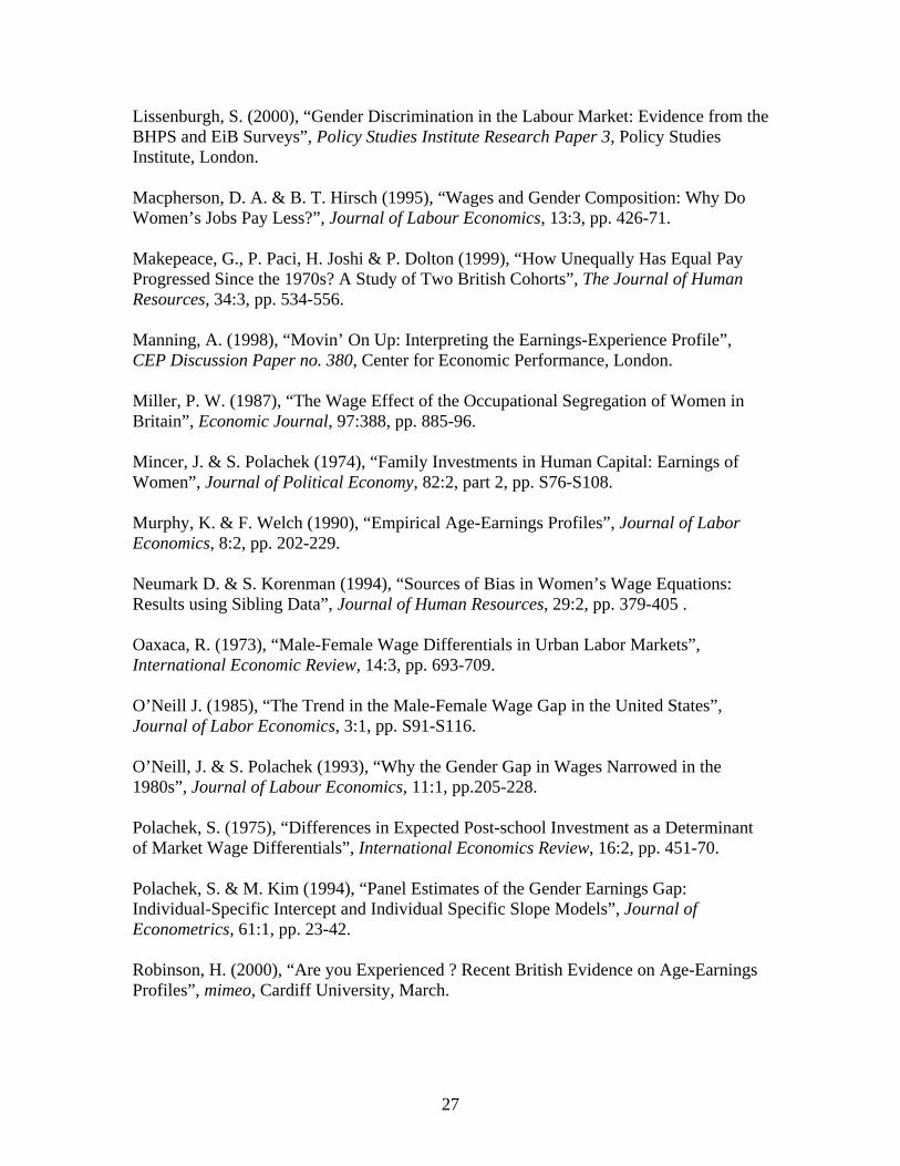
Lissenburgh, S. (2000), “Gender Discrimination in the Labour Market: Evidence from the BHPS and EiB Surveys”, Policy Studies Institute Research Paper 3, Policy Studies Institute, London. Macpherson, D. A. & B. T. Hirsch (1995), “Wages and Gender Composition: Why Do Women’s Jobs Pay Less?”, Journal of Labour Economics, 13:3, pp. 426-71. Makepeace, G., P. Paci, H. Joshi & P. Dolton (1999), “How Unequally Has Equal Pay Progressed Since the 1970s? A Study of Two British Cohorts”, The Journal of Human Resources, 34:3, pp. 534-556. Manning, A. (1998), “Movin’ On Up: Interpreting the Earnings-Experience Profile”, CEP Discussion Paper no. 380, Center for Economic Performance, London. Miller, P. W. (1987), “The Wage Effect of the Occupational Segregation of Women in Britain”, Economic Journal, 97:388, pp. 885-96. Mincer, J. & S. Polachek (1974), “Family Investments in Human Capital: Earnings of Women”, Journal of Political Economy, 82:2, part 2, pp. S76-S108. Murphy, K. & F. Welch (1990), “Empirical Age-Earnings Profiles”, Journal of Labor Economics, 8:2, pp. 202-229. Neumark D. & S. Korenman (1994), “Sources of Bias in Women’s Wage Equations: Results using Sibling Data”, Journal of Human Resources, 29:2, pp. 379-405 . Oaxaca, R. (1973), “Male-Female Wage Differentials in Urban Labor Markets”, International Economic Review, 14:3, pp. 693-709. O’Neill J. (1985), “The Trend in the Male-Female Wage Gap in the United States”, Journal of Labor Economics, 3:1, pp. S91-S116. O’Neill, J. & S. Polachek (1993), “Why the Gender Gap in Wages Narrowed in the 1980s”, Journal of Labour Economics, 11:1, pp.205-228. Polachek, S. (1975), “Differences in Expected Post-school Investment as a Determinant of Market Wage Differentials”, International Economics Review, 16:2, pp. 451-70. Polachek, S. & M. Kim (1994), “Panel Estimates of the Gender Earnings Gap: Individual-Specific Intercept and Individual Specific Slope Models”, Journal of Econometrics, 61:1, pp. 23-42. Robinson, H. (2000), “Are you Experienced ? Recent British Evidence on Age-Earnings Profiles”, mimeo, Cardiff University, March.

27

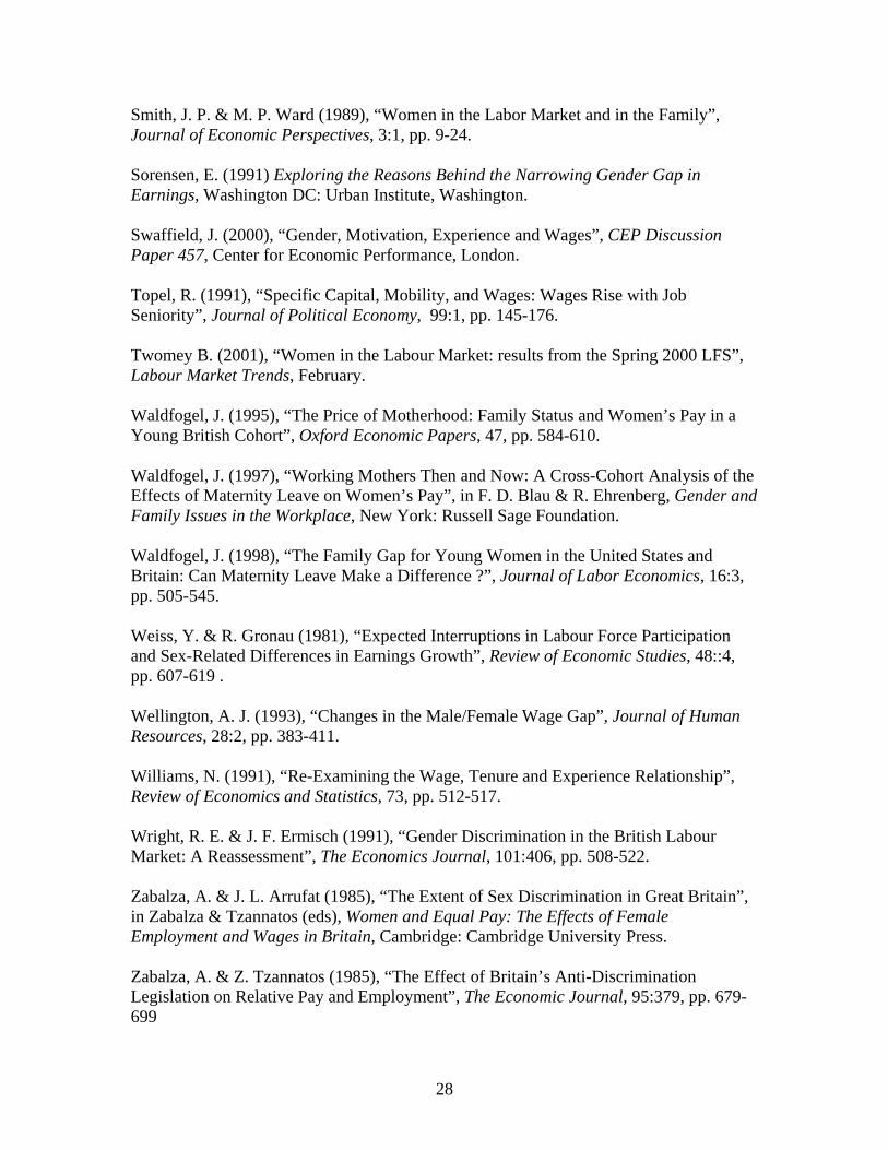
Smith, J. P. & M. P. Ward (1989), “Women in the Labor Market and in the Family”, Journal of Economic Perspectives, 3:1, pp. 9-24. Sorensen, E. (1991) Exploring the Reasons Behind the Narrowing Gender Gap in Earnings, Washington DC: Urban Institute, Washington. Swaffield, J. (2000), “Gender, Motivation, Experience and Wages”, CEP Discussion Paper 457, Center for Economic Performance, London. Topel, R. (1991), “Specific Capital, Mobility, and Wages: Wages Rise with Job Seniority”, Journal of Political Economy, 99:1, pp. 145-176. Twomey B. (2001), “Women in the Labour Market: results from the Spring 2000 LFS”, Labour Market Trends, February. Waldfogel, J. (1995), “The Price of Motherhood: Family Status and Women’s Pay in a Young British Cohort”, Oxford Economic Papers, 47, pp. 584-610. Waldfogel, J. (1997), “Working Mothers Then and Now: A Cross-Cohort Analysis of the Effects of Maternity Leave on Women’s Pay”, in F. D. Blau & R. Ehrenberg, Gender and Family Issues in the Workplace, New York: Russell Sage Foundation. Waldfogel, J. (1998), “The Family Gap for Young Women in the United States and Britain: Can Maternity Leave Make a Difference ?”, Journal of Labor Economics, 16:3, pp. 505-545. Weiss, Y. & R. Gronau (1981), “Expected Interruptions in Labour Force Participation and Sex-Related Differences in Earnings Growth”, Review of Economic Studies, 48::4, pp. 607-619 . Wellington, A. J. (1993), “Changes in the Male/Female Wage Gap”, Journal of Human Resources, 28:2, pp. 383-411. Williams, N. (1991), “Re-Examining the Wage, Tenure and Experience Relationship”, Review of Economics and Statistics, 73, pp. 512-517. Wright, R. E. & J. F. Ermisch (1991), “Gender Discrimination in the British Labour Market: A Reassessment”, The Economics Journal, 101:406, pp. 508-522. Zabalza, A. & J. L. Arrufat (1985), “The Extent of Sex Discrimination in Great Britain”, in Zabalza & Tzannatos (eds), Women and Equal Pay: The Effects of Female Employment and Wages in Britain, Cambridge: Cambridge University Press. Zabalza, A. & Z. Tzannatos (1985), “The Effect of Britain’s Anti-Discrimination Legislation on Relative Pay and Employment”, The Economic Journal, 95:379, pp. 679-699

28

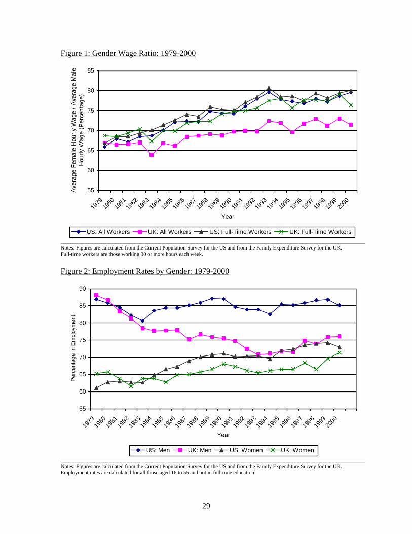
Figure 1: Gender Wage Ratio: 1979-2000

55

60

65

70

75

80

85

1979

1980

1981

1982

1983

1984

1985

1986

1987

1988

1989

1990

1991

1992

1993

1994

1995

1996

1997

1998

1999

2000

Year

Ave

rage

Fem

ale

Hou

rly W

age

/ Ave

rage

Mal

e H

ourly

Wag

e (P

erce

ntag

e)

US: All Workers UK: All Workers US: Full-Time Workers UK: Full-Time Workers

Notes: Figures are calculated from the Current Population Survey for the US and from the Family Expenditure Survey for the UK. Full-time workers are those working 30 or more hours each week.

Figure 2: Employment Rates by Gender: 1979-2000

55

60

65

70

75

80

85

90

1979

1980

1981

1982

1983

1984

1985

1986

1987

1988

1989

1990

1991

1992

1993

1994

1995

1996

1997

1998

1999

2000

Year

Per

cent

age

in E

mpl

oym

ent

US: Men UK: Men US: Women UK: Women

Notes: Figures are calculated from the Current Population Survey for the US and from the Family Expenditure Survey for the UK. Employment rates are calculated for all those aged 16 to 55 and not in full-time education.

29

Figure 3: Employment Rates by Gender and Age

45

50

55

60

65

70

75

80

85

90

95

16 18 20 22 24 26 28 30 32 34 36 38 40 42 44 46 48 50 52 54

Age

Per

cent

age

in E

mpl

oym

ent

US: Men UK: Men US: Women UK: Women

Notes: Figures are calculated from the Current Population Survey for the US and from the Family Expenditure Survey for the UK for the years 1979 to 2000. Employment rates are calculated for all those aged 16 to 55 and not in full-time education.

30

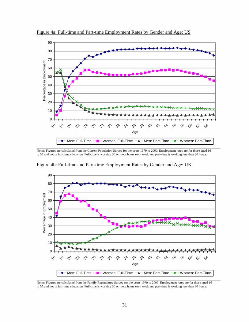
Figure 4a: Full-time and Part-time Employment Rates by Gender and Age: US

0

10

20

30

40

50

60

70

80

90

16 18 20 22 24 26 28 30 32 34 36 38 40 42 44 46 48 50 52 54

Age

Per

cent

age

in E

mpl

oym

ent

Men: Full-Time Women: Full-Time Men: Part-Time Women: Part-Time

Notes: Figures are calculated from the Current Population Survey for the years 1979 to 2000. Employment rates are for those aged 16 to 55 and not in full-time education. Full-time is working 30 or more hours each week and part-time is working less than 30 hours.

Figure 4b: Full-time and Part-time Employment Rates by Gender and Age: UK

0

10

20

30

40

50

60

70

80

90

16 18 20 22 24 26 28 30 32 34 36 38 40 42 44 46 48 50 52 54

Age

Per

cent

age

in E

mpl

oym

ent

Men: Full-Time Women: Full-Time Men: Part-Time Women: Part-Time

Notes: Figures are calculated from the Family Expenditure Survey for the years 1979 to 2000. Employment rates are for those aged 16 to 55 and not in full-time education. Full-time is working 30 or more hours each week and part-time is working less than 30 hours.

31

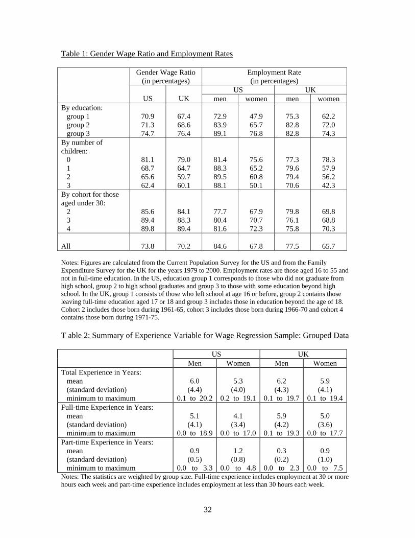
Table 1: Gender Wage Ratio and Employment Rates

Gender Wage Ratio (in percentages)

Employment Rate (in percentages)

US UK

US

UK men women men women

By education: group 1 group 2 group 3

70.9 71.3 74.7

67.4 68.6 76.4

72.9 83.9 89.1

47.9 65.7 76.8

75.3 82.8 82.8

62.2 72.0 74.3

By number of children: 0 1 2 3

81.1 68.7 65.6 62.4

79.0 64.7 59.7 60.1

81.4 88.3 89.5 88.1

75.6 65.2 60.8 50.1

77.3 79.6 79.4 70.6

78.3 57.9 56.2 42.3

By cohort for those aged under 30: 2 3 4

85.6 89.4 89.8

84.1 88.3 89.4

77.7 80.4 81.6

67.9 70.7 72.3

79.8 76.1 75.8

69.8 68.8 70.3

All

73.8

70.2

84.6

67.8

77.5

65.7

Notes: Figures are calculated from the Current Population Survey for the US and from the Family Expenditure Survey for the UK for the years 1979 to 2000. Employment rates are those aged 16 to 55 and not in full-time education. In the US, education group 1 corresponds to those who did not graduate from high school, group 2 to high school graduates and group 3 to those with some education beyond high school. In the UK, group 1 consists of those who left school at age 16 or before, group 2 contains those leaving full-time education aged 17 or 18 and group 3 includes those in education beyond the age of 18. Cohort 2 includes those born during 1961-65, cohort 3 includes those born during 1966-70 and cohort 4 contains those born during 1971-75.

T able 2: Summary of Experience Variable for Wage Regression Sample: Grouped Data

US UK Men Women Men Women

Total Experience in Years: mean (standard deviation) minimum to maximum

6.0

(4.4) 0.1 to 20.2

5.3

(4.0) 0.2 to 19.1

6.2

(4.3) 0.1 to 19.7

5.9

(4.1) 0.1 to 19.4

Full-time Experience in Years: mean (standard deviation) minimum to maximum

5.1

(4.1) 0.0 to 18.9

4.1

(3.4) 0.0 to 17.0

5.9

(4.2) 0.1 to 19.3

5.0

(3.6) 0.0 to 17.7

Part-time Experience in Years: mean (standard deviation) minimum to maximum

0.9

(0.5) 0.0 to 3.3

1.2

(0.8) 0.0 to 4.8

0.3

(0.2) 0.0 to 2.3

0.9

(1.0) 0.0 to 7.5

Notes: The statistics are weighted by group size. Full-time experience includes employment at 30 or more hours each week and part-time experience includes employment at less than 30 hours each week.

32

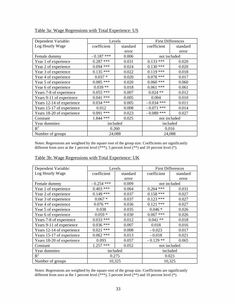
Table 3a: Wage Regressions with Total Experience: US

Levels First Differences Dependent Variable: Log Hourly Wage coefficient standard

error coefficient standard

error Female dummy - 0.187 *** 0.006 not included Year 1 of experience 0.287 *** 0.031 0.133 *** 0.020 Year 2 of experience 0.094 *** 0.024 0.130 *** 0.020 Year 3 of experience 0.135 *** 0.022 0.119 *** 0.018 Year 4 of experience 0.037 * 0.020 0.078 *** 0.017 Year 5 of experience 0.085 *** 0.020 0.060 *** 0.060 Year 6 of experience 0.039 ** 0.018 0.061 *** 0.061 Years 7-8 of experience 0.055 *** 0.007 0.024 ** 0.012 Years 9-11 of experience 0.041 *** 0.005 0.004 0.010 Years 12-14 of experience 0.034 *** 0.005 - 0.034 *** 0.011 Years 15-17 of experience 0.012 0.008 - 0.071 *** 0.014 Years 18-20 of experience 0.091 *** 0.023 - 0.089 *** 0.027 Constant 1.844 *** 0.025 not included Year dummies included included R2 0.260 0.016 Number of groups 24,088 24,088 Notes: Regressions are weighted by the square root of the group size. Coefficients are significantly different from zero at the 1 percent level (***), 5 percent level (**) and 10 percent level (*).

Table 3b: Wage Regressions with Total Experience: UK

Levels First Differences Dependent Variable: Log Hourly Wage coefficient standard

error coefficient standard

error Female dummy - 0.254 *** 0.009 not included Year 1 of experience 0.403 *** 0.064 0.264 *** 0.031 Year 2 of experience 0.149 *** 0.037 0.158 *** 0.027 Year 3 of experience 0.067 * 0.037 0.123 *** 0.027 Year 4 of experience 0.076 ** 0.036 0.121 *** 0.027 Year 5 of experience 0.038 0.035 0.046 * 0.026 Year 6 of experience 0.059 * 0.030 0.067 *** 0.026 Years 7-8 of experience 0.033 *** 0.012 0.041 ** 0.018 Years 9-11 of experience 0.036 *** 0.007 0.018 0.016 Years 12-14 of experience 0.021 *** 0.008 - 0.023 0.017 Years 15-17 of experience 0.062 *** 0.013 - 0.018 0.021 Years 18-20 of experience 0.093 0.057 - 0.129 ** 0.065 Constant 1.257 *** 0.052 not included Year dummies included included R2 0.275 0.023 Number of groups 10,325 10,325 Notes: Regressions are weighted by the square root of the group size. Coefficients are significantly different from zero at the 1 percent level (***), 5 percent level (**) and 10 percent level (*).

33

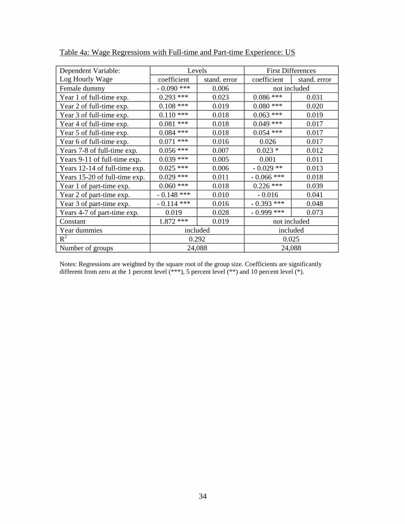
Table 4a: Wage Regressions with Full-time and Part-time Experience: US

Levels First Differences Dependent Variable: Log Hourly Wage coefficient stand. error coefficient stand. error Female dummy - 0.090 *** 0.006 not included Year 1 of full-time exp. 0.293 *** 0.023 0.086 *** 0.031 Year 2 of full-time exp. 0.108 *** 0.019 0.080 *** 0.020 Year 3 of full-time exp. 0.110 *** 0.018 0.063 *** 0.019 Year 4 of full-time exp. 0.081 *** 0.018 0.049 *** 0.017 Year 5 of full-time exp. 0.084 *** 0.018 0.054 *** 0.017 Year 6 of full-time exp. 0.071 *** 0.016 0.026 0.017 Years 7-8 of full-time exp. 0.056 *** 0.007 0.023 * 0.012 Years 9-11 of full-time exp. 0.039 *** 0.005 0.001 0.011 Years 12-14 of full-time exp. 0.025 *** 0.006 - 0.029 ** 0.013 Years 15-20 of full-time exp. 0.029 *** 0.011 - 0.066 *** 0.018 Year 1 of part-time exp. 0.060 *** 0.018 0.226 *** 0.039 Year 2 of part-time exp. - 0.148 *** 0.010 - 0.016 0.041 Year 3 of part-time exp. - 0.114 *** 0.016 - 0.393 *** 0.048 Years 4-7 of part-time exp. 0.019 0.028 - 0.999 *** 0.073 Constant 1.872 *** 0.019 not included Year dummies included included R2 0.292 0.025 Number of groups 24,088 24,088 Notes: Regressions are weighted by the square root of the group size. Coefficients are significantly different from zero at the 1 percent level (***), 5 percent level (**) and 10 percent level (*).

34

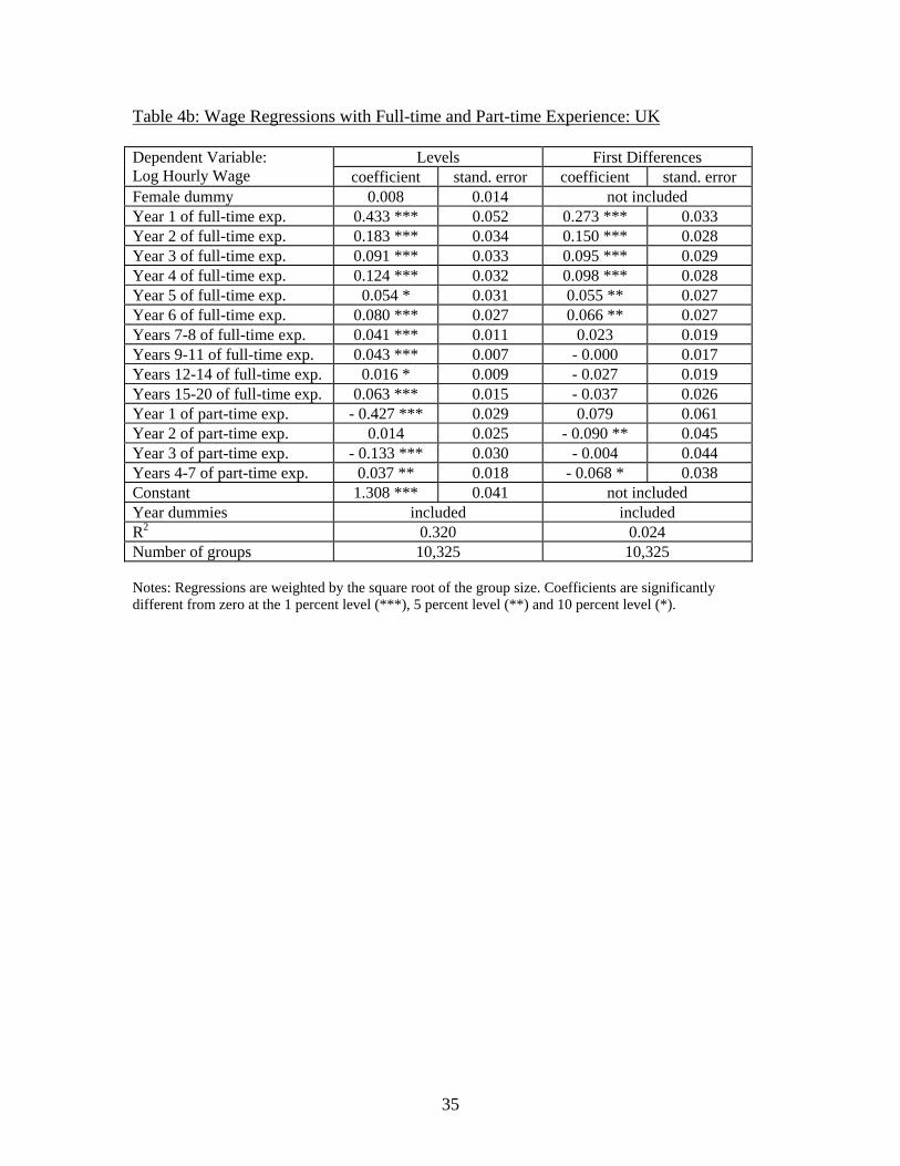
Table 4b: Wage Regressions with Full-time and Part-time Experience: UK

Levels First Differences Dependent Variable: Log Hourly Wage coefficient stand. error coefficient stand. error Female dummy 0.008 0.014 not included Year 1 of full-time exp. 0.433 *** 0.052 0.273 *** 0.033 Year 2 of full-time exp. 0.183 *** 0.034 0.150 *** 0.028 Year 3 of full-time exp. 0.091 *** 0.033 0.095 *** 0.029 Year 4 of full-time exp. 0.124 *** 0.032 0.098 *** 0.028 Year 5 of full-time exp. 0.054 * 0.031 0.055 ** 0.027 Year 6 of full-time exp. 0.080 *** 0.027 0.066 ** 0.027 Years 7-8 of full-time exp. 0.041 *** 0.011 0.023 0.019 Years 9-11 of full-time exp. 0.043 *** 0.007 - 0.000 0.017 Years 12-14 of full-time exp. 0.016 * 0.009 - 0.027 0.019 Years 15-20 of full-time exp. 0.063 *** 0.015 - 0.037 0.026 Year 1 of part-time exp. - 0.427 *** 0.029 0.079 0.061 Year 2 of part-time exp. 0.014 0.025 - 0.090 ** 0.045 Year 3 of part-time exp. - 0.133 *** 0.030 - 0.004 0.044 Years 4-7 of part-time exp. 0.037 ** 0.018 - 0.068 * 0.038 Constant 1.308 *** 0.041 not included Year dummies included included R2 0.320 0.024 Number of groups 10,325 10,325 Notes: Regressions are weighted by the square root of the group size. Coefficients are significantly different from zero at the 1 percent level (***), 5 percent level (**) and 10 percent level (*).

35

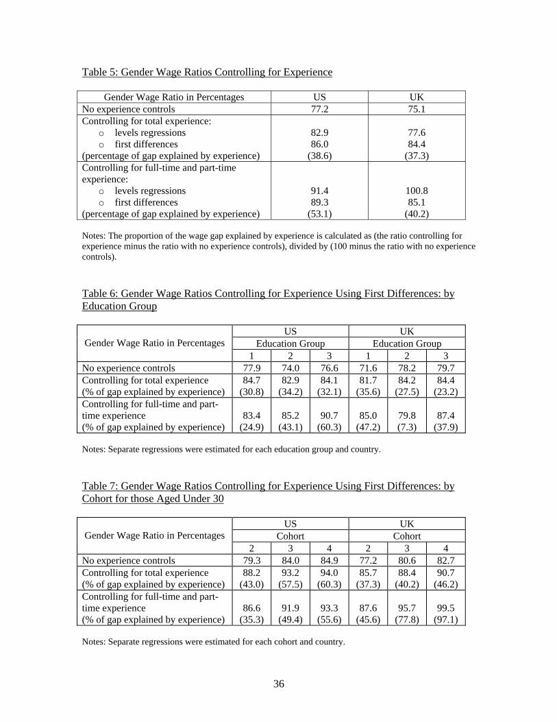
Table 5: Gender Wage Ratios Controlling for Experience

Gender Wage Ratio in Percentages US UK No experience controls 77.2 75.1 Controlling for total experience:

o levels regressions o first differences

(percentage of gap explained by experience)

82.9 86.0

(38.6)

77.6 84.4

(37.3) Controlling for full-time and part-time experience:

o levels regressions o first differences

(percentage of gap explained by experience)

91.4 89.3

(53.1)

100.8 85.1

(40.2) Notes: The proportion of the wage gap explained by experience is calculated as (the ratio controlling for experience minus the ratio with no experience controls), divided by (100 minus the ratio with no experience controls).

Table 6: Gender Wage Ratios Controlling for Experience Using First Differences: by Education Group

US UK Education Group Education Group

Gender Wage Ratio in Percentages

1 2 3 1 2 3 No experience controls 77.9 74.0 76.6 71.6 78.2 79.7 Controlling for total experience (% of gap explained by experience)

84.7 (30.8)

82.9 (34.2)

84.1 (32.1)

81.7 (35.6)

84.2 (27.5)

84.4 (23.2)

Controlling for full-time and part-time experience (% of gap explained by experience)

83.4

(24.9)

85.2

(43.1)

90.7

(60.3)

85.0

(47.2)

79.8 (7.3)

87.4

(37.9) Notes: Separate regressions were estimated for each education group and country. Table 7: Gender Wage Ratios Controlling for Experience Using First Differences: by Cohort for those Aged Under 30

US UK Cohort Cohort

Gender Wage Ratio in Percentages

2 3 4 2 3 4 No experience controls 79.3 84.0 84.9 77.2 80.6 82.7 Controlling for total experience (% of gap explained by experience)

88.2 (43.0)

93.2 (57.5)

94.0 (60.3)

85.7 (37.3)

88.4 (40.2)

90.7 (46.2)

Controlling for full-time and part-time experience (% of gap explained by experience)

86.6

(35.3)

91.9

(49.4)

93.3

(55.6)

87.6

(45.6)

95.7

(77.8)

99.5

(97.1) Notes: Separate regressions were estimated for each cohort and country.

36

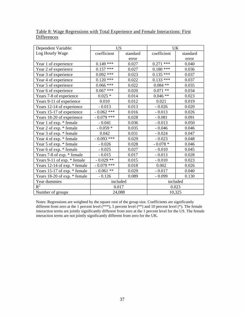
Table 8: Wage Regressions with Total Experience and Female Interactions: First Differences

US UK Dependent Variable: Log Hourly Wage coefficient standard

error coefficient standard

error Year 1 of experience 0.149 *** 0.027 0.271 *** 0.040 Year 2 of experience 0.157 *** 0.027 0.180 *** 0.036 Year 3 of experience 0.092 *** 0.023 0.135 *** 0.037 Year 4 of experience 0.120 *** 0.022 0.133 *** 0.037 Year 5 of experience 0.066 *** 0.022 0.084 ** 0.035 Year 6 of experience 0.067 *** 0.020 0.071 ** 0.034 Years 7-8 of experience 0.025 * 0.014 0.046 ** 0.023 Years 9-11 of experience 0.010 0.012 0.021 0.019 Years 12-14 of experience - 0.013 0.013 - 0.026 0.020 Years 15-17 of experience - 0.062 *** 0.016 - 0.013 0.026 Years 18-20 of experience - 0.079 *** 0.028 - 0.081 0.091 Year 1 of exp. * female - 0.041 0.036 - 0.013 0.050 Year 2 of exp. * female - 0.059 * 0.035 - 0.046 0.046 Year 3 of exp. * female 0.042 0.031 - 0.024 0.047 Year 4 of exp. * female - 0.093 *** 0.029 - 0.023 0.048 Year 5 of exp. * female - 0.026 0.028 - 0.078 * 0.046 Year 6 of exp. * female - 0.025 0.027 - 0.010 0.045 Years 7-8 of exp. * female - 0.015 0.017 - 0.013 0.028 Years 9-11 of exp. * female - 0.029 ** 0.015 - 0.010 0.023 Years 12-14 of exp. * female - 0.079 *** 0.018 0.002 0.026 Years 15-17 of exp. * female - 0.061 ** 0.029 - 0.017 0.040 Years 18-20 of exp. * female - 0.126 0.089 - 0.099 0.130 Year dummies included included R2 0.017 0.023 Number of groups 24,088 10,325 Notes: Regressions are weighted by the square root of the group size. Coefficients are significantly different from zero at the 1 percent level (***), 5 percent level (**) and 10 percent level (*). The female interaction terms are jointly significantly different from zero at the 1 percent level for the US. The female interaction terms are not jointly significantly different from zero for the UK.

37

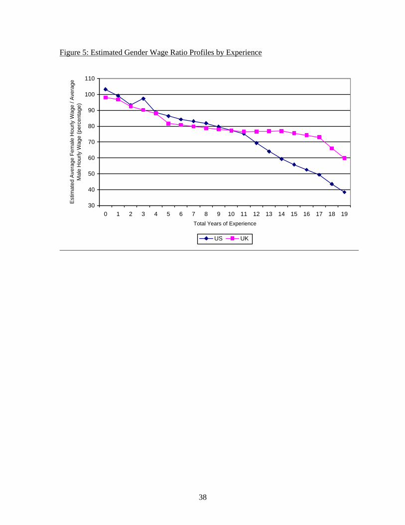
Figure 5: Estimated Gender Wage Ratio Profiles by Experience

30

40

50

60

70

80

90

100

110

0 1 2 3 4 5 6 7 8 9 10 11 12 13 14 15 16 17 18 19Total Years of Experience

Est

imat

ed A

vera

ge F

emal

e H

ourly

Wag

e / A

vera

ge

Mal

e H

ourly

Wag

e (p

erce

ntag

e)

US UK

38

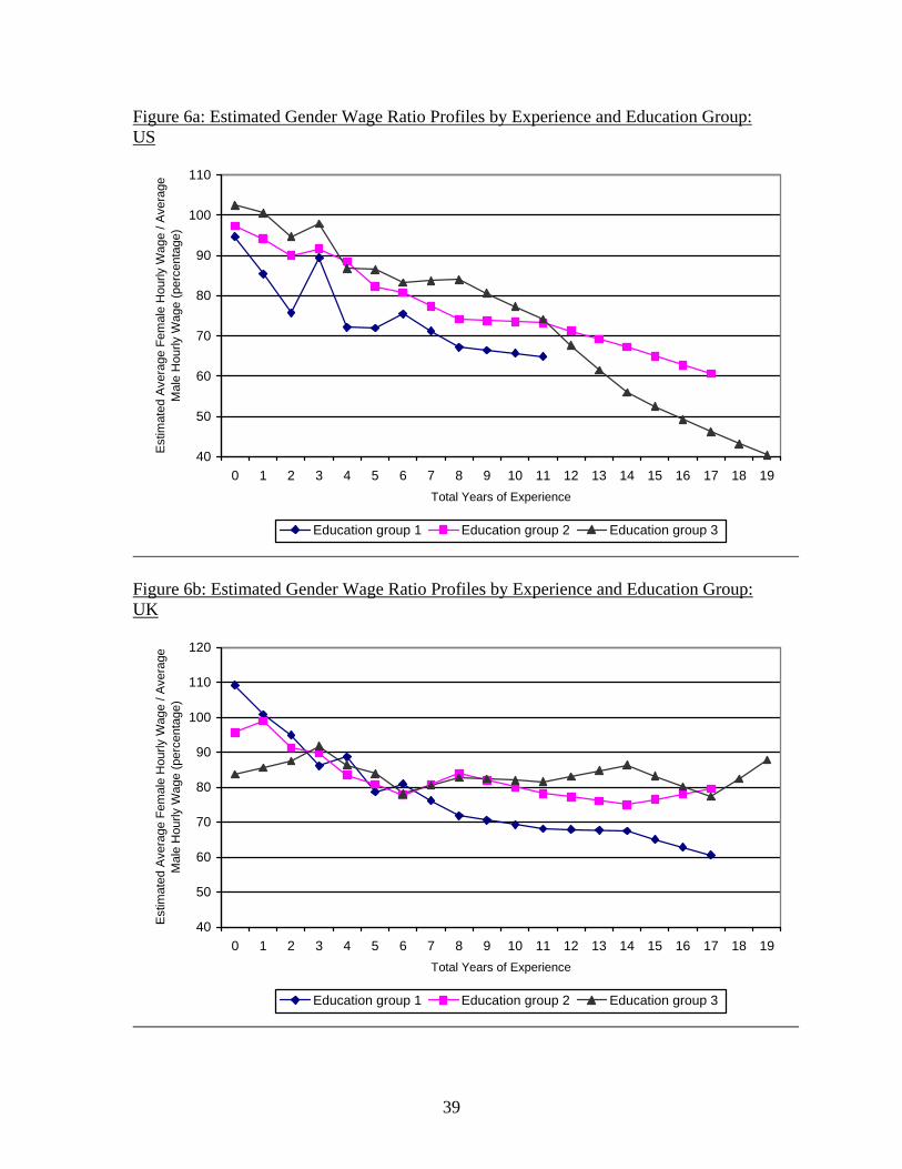
Figure 6a: Estimated Gender Wage Ratio Profiles by Experience and Education Group: US

40

50

60

70

80

90

100

110

0 1 2 3 4 5 6 7 8 9 10 11 12 13 14 15 16 17 18 19Total Years of Experience

Est

imat

ed A

vera

ge F

emal

e H

ourly

Wag

e / A

vera

ge

Mal

e H

ourly

Wag

e (p

erce

ntag

e)

Education group 1 Education group 2 Education group 3

Figure 6b: Estimated Gender Wage Ratio Profiles by Experience and Education Group: UK

40

50

60

70

80

90

100

110

120

0 1 2 3 4 5 6 7 8 9 10 11 12 13 14 15 16 17 18 19Total Years of Experience

Est

imat

ed A

vera

ge F

emal

e H

ourly

Wag

e / A

vera

ge

Mal

e H

ourly

Wag

e (p

erce

ntag

e)

Education group 1 Education group 2 Education group 3

39

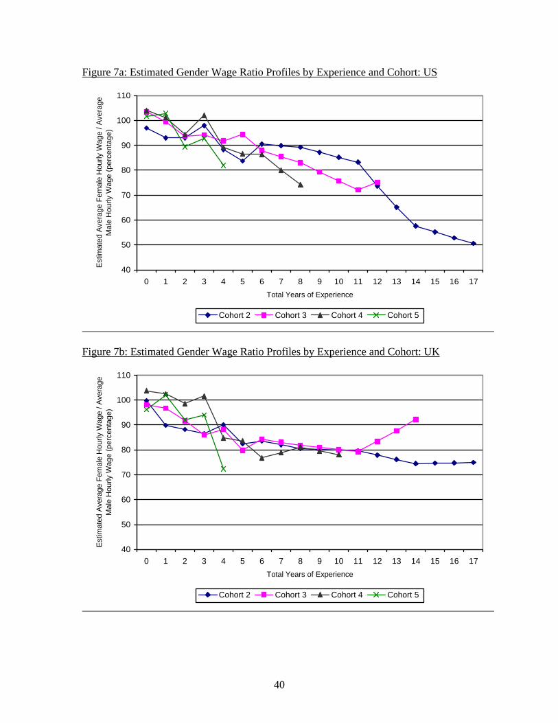
Figure 7a: Estimated Gender Wage Ratio Profiles by Experience and Cohort: US

40

50

60

70

80

90

100

110

0 1 2 3 4 5 6 7 8 9 10 11 12 13 14 15 16 17Total Years of Experience

Est

imat

ed A

vera

ge F

emal

e H

ourly

Wag

e / A

vera

ge

Mal

e H

ourly

Wag

e (p

erce

ntag

e)

Cohort 2 Cohort 3 Cohort 4 Cohort 5

Figure 7b: Estimated Gender Wage Ratio Profiles by Experience and Cohort: UK

40

50

60

70

80

90

100

110

0 1 2 3 4 5 6 7 8 9 10 11 12 13 14 15 16 17Total Years of Experience

Est

imat

ed A

vera

ge F

emal

e H

ourly

Wag

e / A

vera

ge

Mal

e H

ourly

Wag

e (p

erce

ntag

e)

Cohort 2 Cohort 3 Cohort 4 Cohort 5

40