PROCEEDINGS OF THEROMAN NUMBER THEORY ASSOCIATIONVolume 2, Number 1, March 2017, pages 61-81

Michel Waldschmidt

Continued Fractions:Introduction and Applications

written by Carlo Sanna

The continued fraction expansion of a real number x is a very efficientprocess for finding the best rational approximations of x. Moreover,continued fractions are a very versatile tool for solving problems relatedwith movements involving two different periods. This situation occursboth in theoretical questions of number theory, complex analysis, dy-namical systems... as well as in more practical questions related withcalendars, gears, music... We will see some of these applications.

1 The algorithm of continued fractions

Given a real number x, there exist an unique integer bxc, called theintegral part of x, and an unique real {x} ∈ [0, 1[, called the fractionalpart of x, such that

x = bxc + {x}.

If x is not an integer, then {x} , 0 and setting x1 := 1/{x} we have

x = bxc +1x1.

61

Again, if x1 is not an integer, then {x1} , 0 and setting x2 := 1/{x1}

we get

x = bxc +1

bx1c +1x2

.

This process stops if for some i it occurs {xi } = 0, otherwise it continuesforever. Writing a0 := bxc and ai = bxic for i ≥ 1, we obtain the so-called continued fraction expansion of x:

x = a0 +1

a1 +1

a2 +1

a3 +. . .

,

which from now on we will write with the more succinct notation

x = [a0, a1, a2, a3, . . .].

The integers a0, a1, . . . are called partial quotients of the continuedfraction of x, while the rational numbers

pkqk

:= [a0, a1, a2, . . . , ak]

are called convergents. The convergents are the best rational approxi-mations of x in the following sense: If p and q > 0 are integers suchthat �����

pq− x

�����<

12q2 , (1)

then p/q is a convergent of x. Indeed, of any two consecutive con-vergents pk/qk and pk+1/qk+1 of x, one at least satisfies (1) (see [7,Theorems 183 and 184]).If x = a/b is a rational number, then the method for obtaining the

continued fraction of x is nothing else than the Euclidean algorithm for

62

computing the greatest common divisor of a and b:

a = a0b + r0, 0 ≤ r0 < b, x1 = b/r0,

b = a1r0 + r1, 0 ≤ r1 < r0, x2 = r0/r1,

r0 = a2r1 + r2, 0 ≤ r2 < r1, x3 = r1/r2,

· · ·

Therefore, on the one hand, since the Euclidean algorithm alwaysstops, the continued fraction of a rational number is always finite. Onthe other hand, it is obvious that a finite continued fraction representsa rational number. Hence, in conclusion, we have shown that a realnumber is rational if and only if its continued fraction expansion isfinite.Note that, if ak ≥ 2, then

[a0, a1, a2, . . . , ak] = [a0, a1, a2, . . . , ak−1, ak − 1, 1], (2)

Thus a rational number can be expressed as a continued fraction in atleast two ways. Indeed, it can be proved [7, Theorem 162] that anyrational number can be written as a continued fraction in exactly twoways, which are given by (2).

2 The number of days in a year

Let us see an application of continued fractions to the design of acalendar. How many days are in a year? A good answer is 365.However, the astronomers tell us that the Earth completes its orbitaround the Sun in approximately 365.2422 days. The continued fractionof this figure is

365.2422 = [365, 4, 7, 1, 3, 4, 1, 1, 1, 2].

The second convergent is

365.25 = 365 +14,

63

which means a calendar of 365 days per year but a leap year every 4years. The forth convergent gives the better approximation

365.2424 . . . = [365, 4, 7, 1] = 365 +833.

The Gregorian calendar, named after Pope Gregorio XIII who intro-duced it in 1582, is based on a cycle of 400 years: there is one leap yearevery year which is a multiple of 4 but not of 100 unless it is a multipleof 400. This means that in 400 years one omits 3 leap years, thus thereare

400 · 365 + 100 − 3 = 146097

days. On the other hand, in 400 years the number of days counted withan year of 365 + 8

33 days is

400 ·(365 +

833

)= 146096.9696 . . .

a very good approximation!

3 Design a planetarium

Christiaan Huygens (1629–1695) among being a mathematician, as-tronomer, physicist and probabilist, was also a great horologist. Hedesigned more accurate clocks then the ones available at his time. Inparticular, his invention of the pendulum clock was a breakthrough intimekeeping. Huygens also built a mechanical model of the solar sys-tem. He wanted to design the gear ratios in order to produce a properscaled version of the planetary orbits. He knew that the time requiredfor the planet Saturn to orbit around the Sun is about

777084312640858

= 29.425448 . . . = [29, 2, 2, 1, 5, 1, 4, . . .].

The forth convergent is

[29, 2, 2, 1] =2067.

64

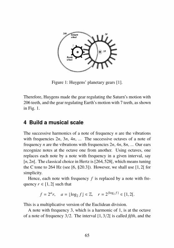
Figure 1: Huygens’ planetary gears [1].

Therefore, Huygens made the gear regulating the Saturn’s motion with206 teeth, and the gear regulating Earth’s motion with 7 teeth, as shownin Fig. 1.

4 Build a musical scale

The successive harmonics of a note of frequency n are the vibrationswith frequencies 2n, 3n, 4n, ... The successive octaves of a note offrequency n are the vibrations with frequencies 2n, 4n, 8n, ... Our earsrecognize notes at the octave one from another. Using octaves, onereplaces each note by a note with frequency in a given interval, say[n, 2n[. The classical choice in Hertz is [264, 528[, which means tuningthe C tone to 264 Hz (see [6, §20.3]). However, we shall use [1, 2[ forsimplicity.Hence, each note with frequency f is replaced by a note with fre-

quency r ∈ [1, 2[ such that

f = 2ar, a = blog2 f c ∈ Z, r = 2{log2 f } ∈ [1, 2[.

This is a multiplicative version of the Euclidean division.A note with frequency 3, which is a harmonic of 1, is at the octave

of a note of frequency 3/2. The interval [1, 3/2[ is called fifth, and the

65

ratio of its end points is 3/2. The interval [3/2, 2[ is called fourth, withratio 4/3. The successive fifths are the notes in the interval [1, 2[ whichare at the octave of notes with frequencies

1, 3, 9, 27, 81, . . .

namely:

1,32,98,2716,8164, . . .

We shall never come back to the initial value 1, since the Diophantineequation 2a = 3b has no solution in integers a and b.In other words, the logarithm of 3 in basis 2 is irrational. Powers of 2

which are close to power of 3 correspond to good rational approximationa/b to log2 3. Thus it is natural to look at the continued fractionexpansion:

log2 3 = 1.58496250072 . . . = [1, 1, 1, 2, 2, 3, 1, 5, . . .].

The approximation

log2 3 ≈ [1, 1, 1, 2] =85

means that 28 = 256 is not too far from 35 = 243, that is, 5 fifthsproduce almost 3 octaves. The next approximation

log2 3 ≈ [1, 1, 1, 2, 2] =1912

tells us that 219 = 524288 is close to 312 = 531441, that is(32

)12= 129.74 . . . ≈ 27 = 128.

This means that 12 fifths are just a bit more than 7 octaves.The figure

312

219 = 1.01364,

66

is called the Pythagorean comma (or ditonic comma) and produces anerror of about 1.36%, which most people cannot hear.Further remarkable approximations between perfect powers are:

53 = 125 ≈ 27 = 128,

that is, (54

)3= 1.953 . . . ≈ 2,

so that 3 thirds (ratio 5/4) produce almost 1 octave; and

210 = 1024 ≈ 103,

which means that one kibibyte (1024 bytes) is about one kilobyte (1000bytes), and that doubling the intensity of a sound is close to adding 3decibels.

5 Exponential Diophantine equations

Another way to avoid the problem that we cannot solve the equation2a = 3b in positive integers a and b, might be looking for powersof 2 which are just one unit from powers of 3, that is |2a − 3b | = 1.This question was asked by the French composer Philippe de Vitry(1291–1361) to the medieval Jewish philosopher and astronomer Leviben Gershon (1288–1344). Gershon proved that there are only threesolutions (a, b) to the Diophantine equation 2a − 3b = ±1, namely(1, 1), (2, 1), (3, 2).Indeed, suppose that 2a − 3b = −1. If a = 1 then, obviously, b = 1.

If a ≥ 2 then 3b ≡ 1 (mod 4), so that b = 2k for some positive integerk, and consequently

2a = 3b − 1 = (3k − 1)(3k + 1),

which implies that both 3k − 1 and 3k + 1 are powers of 2. But the onlypowers of 2 which differ by 2 are 2 and 4, hence k = 1, b = 2, anda = 3.

67

Similarly, suppose that 2a − 3b = 1. Hence 2a ≡ 1 (mod 3), so thata = 2k for some positive integer k and

3b = 2a − 1 = (2k − 1)(2k + 1),

which implies that both 2k − 1 and 2k + 1 are powers of 3. But the onlypowers of 3 which differ by 2 are 1 and 3, hence k = 1, a = 2, andb = 1.This kind of questions lead to the study of the so called exponential

Diophantine equations. A notable case is the Catalan’s equation

xp − yq = 1,

where x, y, p, q are integers all ≥ 2. In 2002 Mihăilescu [9] showedthat 32 − 23 = 1 is the only solution, as conjectured by Catalan in 1844.

6 Electric networks

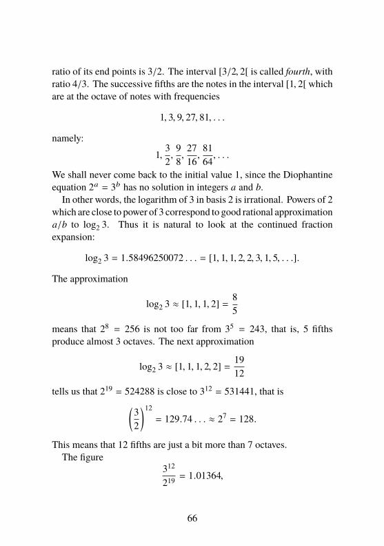
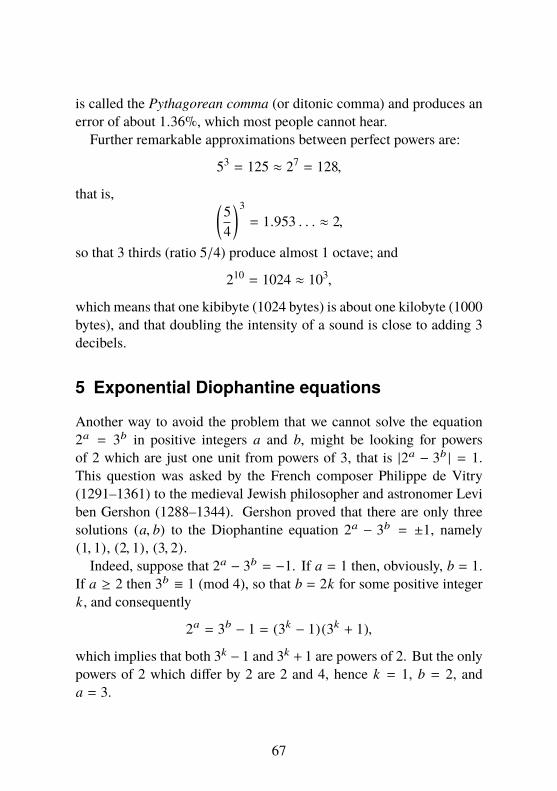
The electrical resistance of a series of two resistances R1 and R2 isR1 + R2 (see Fig. 2). If R1 and R2 are instead in a parallel network (see

Figure 2: Two resistances R1 and R2 in series.

Fig. 3), then the resulting resistance R satisfies

1R=

1R1+

1R2.

Therefore, it follows easily that the resistance U of the circuit of Fig. 4

68

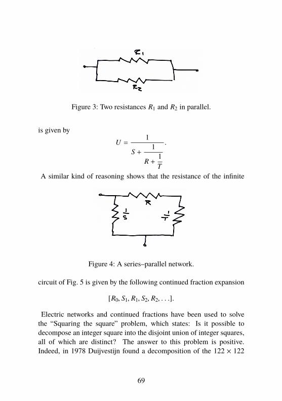
Figure 3: Two resistances R1 and R2 in parallel.

is given by

U =1

S +1

R +1T

.

A similar kind of reasoning shows that the resistance of the infinite

Figure 4: A series–parallel network.

circuit of Fig. 5 is given by the following continued fraction expansion

[R0, S1, R1, S2, R2, . . .].

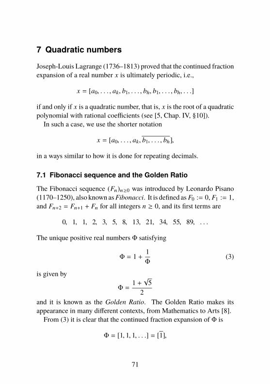
Electric networks and continued fractions have been used to solvethe “Squaring the square” problem, which states: Is it possible todecompose an integer square into the disjoint union of integer squares,all of which are distinct? The answer to this problem is positive.Indeed, in 1978 Duijvestijn found a decomposition of the 122 × 122

69

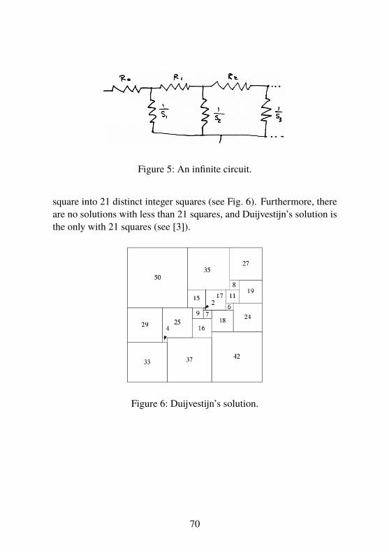
Figure 5: An infinite circuit.

square into 21 distinct integer squares (see Fig. 6). Furthermore, thereare no solutions with less than 21 squares, and Duijvestijn’s solution isthe only with 21 squares (see [3]).

Figure 6: Duijvestijn’s solution.

70

7 Quadratic numbers

Joseph-Louis Lagrange (1736–1813) proved that the continued fractionexpansion of a real number x is ultimately periodic, i.e.,

x = [a0, . . . , ak, b1, . . . , bh, b1, . . . , bh, . . .]

if and only if x is a quadratic number, that is, x is the root of a quadraticpolynomial with rational coefficients (see [5, Chap. IV, §10]).In such a case, we use the shorter notation

x = [a0, . . . , ak, b1, . . . , bh],

in a ways similar to how it is done for repeating decimals.

7.1 Fibonacci sequence and the Golden Ratio

The Fibonacci sequence (Fn)n≥0 was introduced by Leonardo Pisano(1170–1250), also known asFibonacci. It is defined as F0 := 0, F1 := 1,and Fn+2 = Fn+1 + Fn for all integers n ≥ 0, and its first terms are

0, 1, 1, 2, 3, 5, 8, 13, 21, 34, 55, 89, . . .

The unique positive real numbers Φ satisfying

Φ = 1 +1Φ

(3)

is given by

Φ =1 +√

52

and it is known as the Golden Ratio. The Golden Ratio makes itsappearance in many different contexts, from Mathematics to Arts [8].From (3) it is clear that the continued fraction expansion of Φ is

Φ = [1, 1, 1, . . .] = [1],

71

the simplest infinite continued fraction. Notably, the convergents of Φare precisely the ratios of consecutive Fibonacci numbers

[1] =F2

F1, [1, 1] =

F3

F2, [1, 1, 1] =

F4

F3, [1, 1, 1, 1] =

F5

F4, . . .

so thatΦ = lim

n→+∞

Fn+1

Fn.

7.2 Continued fraction for√

2

The square root of 2 satisfies

√2 = 1 +

1√

2 + 1,

while√

2 = 1 +1

2 +1

√2 + 1

,

hence the continued fraction expansion of√

2 is given by√

2 = [1, 2, 2, 2, . . .] = [1, 2].

7.3 Paper folding

The number√

2 appears in the A series paper sizes. Precisely, since√

2is twice its inverse, i.e.,

√2 = 2/

√2, folding a rectangular piece of paper

with sides in proportion√

2 yields a new rectangular piece of paper withsides in proportion

√2 again. The sizes of an A0 paper are defined to

be in proportion√

2 and so that the area is 1 m2. Thus, rounded to thenearest millimetre, an A0 paper is 841 by 1189 millimetres. Note that

8411189

=2949= [1, 2, 2, 2, 2]

72

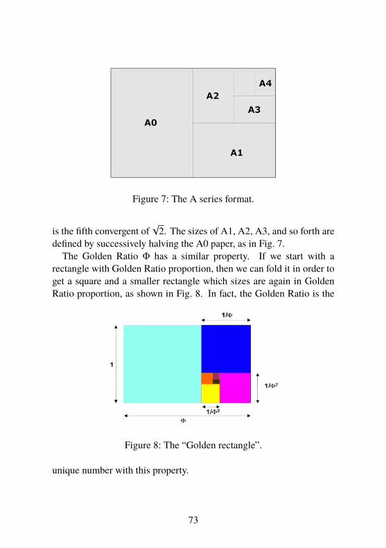
Figure 7: The A series format.

is the fifth convergent of√

2. The sizes of A1, A2, A3, and so forth aredefined by successively halving the A0 paper, as in Fig. 7.

The Golden Ratio Φ has a similar property. If we start with arectangle with Golden Ratio proportion, then we can fold it in order toget a square and a smaller rectangle which sizes are again in GoldenRatio proportion, as shown in Fig. 8. In fact, the Golden Ratio is the

Figure 8: The “Golden rectangle”.

unique number with this property.

73

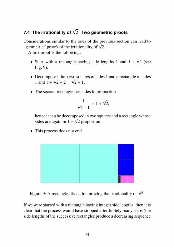
7.4 The irrationality of√

2: Two geometric proofs

Considerations similar to the ones of the previous section can lead to“geometric” proofs of the irrationality of

√2.

A first proof is the following:

• Start with a rectangle having side lengths 1 and 1 +√

2 (seeFig. 9).

• Decompose it into two squares of sides 1 and a rectangle of sides1 and 1 +

√2 − 2 =

√2 − 1.

• The second rectangle has sides in proportion

1√

2 − 1= 1 +

√2,

hence it can be decomposed in two squares and a rectangle whosesides are again in 1 +

√2 proportion.

• This process does not end.

Figure 9: A rectangle dissection proving the irrationality of√

2.

If we were started with a rectangle having integer side lengths, then it isclear that the process would have stopped after finitely many steps (theside lengths of the successive rectangles produce a decreasing sequence

74

of positive integers). The same conclusion holds for a rectangle withside lengths in rational proportion (reduce to a common denominatorand scale). Therefore, 1 +

√2 is irrational, and so is

√2.

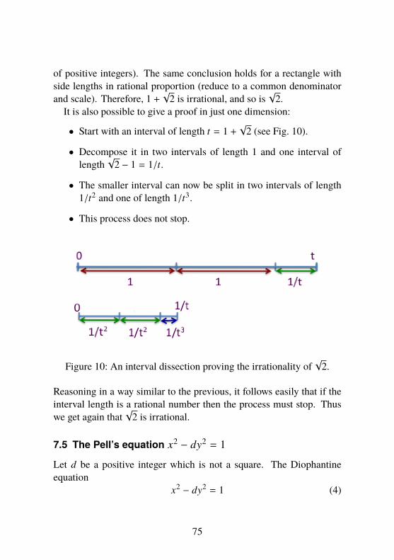
It is also possible to give a proof in just one dimension:

• Start with an interval of length t = 1 +√

2 (see Fig. 10).

• Decompose it in two intervals of length 1 and one interval oflength

√2 − 1 = 1/t.

• The smaller interval can now be split in two intervals of length1/t2 and one of length 1/t3.

• This process does not stop.

Figure 10: An interval dissection proving the irrationality of√

2.

Reasoning in a way similar to the previous, it follows easily that if theinterval length is a rational number then the process must stop. Thuswe get again that

√2 is irrational.

7.5 The Pell’s equation x2 − dy2 = 1

Let d be a positive integer which is not a square. The Diophantineequation

x2 − dy2 = 1 (4)

75

is known as Pell’s equation [5, Chap. IV, §11]. It can be rewritten as(x −√

dy) (

x +√

dy)= 1,

hence, for y > 0, we have that x/y is a rational approximation of√d. This is the reason why a strategy for solving (4) is based on the

continued fraction expansion of√

d.It is quite curious that for relatively small values of d the solutions

(x, y) of (4) can be very large. For example, the Indian mathematicianBrahmagupta (~628) asked for solution for d = 92. The continuedfraction expansion of

√92 is

√92 = [9, 1, 1, 2, 4, 2, 1, 1, 18],

and a solution (x, y) = (1151, 120) is obtained from

[9, 1, 1, 2, 4, 2, 1, 1] =1151120

.

Another example is the one of Bhaskara (~1150), that using the samemethod of Brahmagupta showed that a solution for d = 61 is given by

x = 1766319049, y = 226153980.

But a more impressive example was given by Fermat, who asked to hisfriend Brouncker a solution for d = 109, saying that he choose a smallvalue of d to make the problem not too difficult. However, the smallestsolution is

x = 158070671986249, y = 15140424455100,

which is also given by

*,

261 + 25√

1092

+-

6

= 158070671986249 + 15140424455100√

109.

76

8 Continued fractions for e and π

Leonard Euler (1707–1784) proved that the continued fraction for e isgiven by

e = [2, 1, 2, 1, 1, 4, 1, 1, 6, 1, . . .]

= [2, 1, 2m, 1]m≥1.

This result implies that e is not rational neither a quadratic irrational.(Indeed, in 1874 Charles Hermite proved that e is transcendental.)Actually, Euler showed the more general result that for any integera ≥ 1 it holds

e1/a = [1, a − 1, 1, 3a − 1, 1, 1, 5a − 1, 1, . . .]

= [1, (2m + 1)a − 1, 1]m≥1.

JohannHeinrich Lambert (1728–1777) proved tan(v) is irrational whenv , 0 is rational. Hence π is irrational, since tan(π/4) = 1. Thecontinued fraction expansion of π,

π = [3, 7, 15, 1, 292, 1, 1, 1, 2, 1, 3, 1, 14, 2, 1, 1, . . .].

is much more mysterious than the one of e. Indeed, it is still anopen problem to understand if the sequence of partial quotients of π isbounded or not.

9 Continued fractions for analytic functions

Also some analytic functions have a kind of continued fraction expan-sion. For example, the tangent:

tan(x) =x

1 −x2

3 −x2

5 −x2

7 − . . .

.

77

The study of continued fractions of analytic functions is strictly con-nected to the theory of Padé approximations, which are rational functionapproximations of analytic functions (see [4]).

10 Gauss map and ergodic theory

Let (X, µ) be a probability space and let H : X → X be a map thatpreserve the measure µ, i.e., µ(H−1(E)) = µ(E) for any measurableE ⊆ X . The Birkhoff’s Ergodic Theorem [13, §1.6] states that if H isergodic, which means that H−1(E) = E implies µ(E) = 0 or µ(E) = 1,then for any f ∈ L1

µ (X ) we have

limn→∞

1n

n∑k=1

f (H (k) (x)) =∫X

f dµ,

for almost all x ∈ X , respect to the measure µ, where H (k) denotes thek-th iterate of H .We have seen that the partial quotient of a continued fraction are

obtained by iterating the map

T : x 7→1x−

⌊1x

⌋,

which is called Gauss map. It can be proved that the Gauss mappreserve the measure

µ(E) :=1

log 2

∫E

dxx + 1

, E ⊆ [0, 1],

and that it is ergodic. This facts connect continued fractions with thestudy of chaotic dynamical systems. In particular, exploiting this con-nection, it can be proved the following result of Aleksandr YakovlevichKhinchin: For all real numbers

x = [a0, a1, a2, . . .],

78

but a set of Lebesgue measure zero, it holds

limn→∞

n

√√n∏

k=1ak = K0,

where

K0 :=∞∏r=1

(1 +

1r (r + 2)

) log2 r

≈ 2.685452 . . .

is known as Khinchin’s constant.

11 Connection with the Riemann zeta function

We recall that for real s > 1, the Riemann zeta function is defined by

ζ (s) =∞∑n=1

1ns.

Notably, ζ (s) is related to the Gauss map T by the following formula

ζ (s) =1

s − 1− s

∫ 1

0T (x)xs−1ds.

12 Generalizations of continued expansion inhigher dimension

Simultaneous rational approximations of real numbers is a much moredifficult problem than the rational approximation of a single number.In fact, the continued fraction expansion algorithm has many specificfeatures and so far there is no extension of this algorithm in higherdimension with all such properties.However, some attempts has been made, in particular the Jacobi–

Perron algorithm [2] uses a kind of ternary continued fraction expansion

79

to deal with cubic irrationality. This topic is strictly related the Geom-etry of numbers, started by Hermann Minkowski (1864–1909), whichis the study of convex bodies and integer vectors in the n-dimensionalspace Rn. One of the most important result of this field is the LLLalgorithm [10], named after Arjen Lenstra, Hendrik Lenstra and LaszloLovasz, that given m vectors in Rn it produces a basis of the lattice theygenerate with often a smaller norm than the initial ones.For more recent results see the works of Wolfgang Schmidt, Leon-

hard Summerer, and Damien Roy [11, 12] in the so-called Parametricgeometry of numbers.

References

[1] Chaos in Numberland: The secret life of contin-ued fractions, http://plus.maths.org/content/chaos-numberland-secret-life-continued-fractions.

[2] L. Bernstein, The Jacobi-Perron algorithm—Its theory and appli-cation, Lecture Notes in Mathematics, Vol. 207, Springer-Verlag,Berlin-New York, 1971.

[3] C. J. Bouwkamp and A. J. W. Duijvestijn, Catalogue of simpleperfect squared squares of orders 21 through 25, EUT Report-WSK, vol. 92, Eindhoven University of Technology, Departmentof Mathematics and Computing Science, Eindhoven, 1992.

[4] C. Brezinski, History of continued fractions and Padé approxi-mants, Springer Series in Computational Mathematics, vol. 12,Springer-Verlag, Berlin, 1991.

[5] H. Davenport, The Higher Arithmetic, eighth ed., Cambridge Uni-versity Press, Cambridge, 2008, An introduction to the theory ofnumbers, With editing and additional material by James H. Dav-enport.

80

[6] P. U. P. A. Gilbert and W. Haeberli, Physics in the Arts: Revisededition, Complementary Science, Elsevier Science, 2011.

[7] G. H. Hardy and E. M. Wright, An introduction to the theory ofnumbers, sixth ed., Oxford University Press, Oxford, 2008, Re-vised by D. R. Heath-Brown and J. H. Silverman, With a forewordby Andrew Wiles.

[8] H. E. Huntley, The Divine Proportion: A Study in MathematicalBeauty, Dover Books on Mathematics, Dover Publications, 1970.

[9] P. Mihăilescu, Primary cyclotomic units and a proof of Catalan’sconjecture, J. Reine Angew. Math. 572 (2004), 167–195.

[10] P. Q. Nguyen andB. Vallée (eds.), The LLL algorithm: Survey andapplications, Information Security and Cryptography, Springer-Verlag Berlin Heidelberg, 2010.

[11] D. Roy, On Schmidt and Summerer parametric geometry of num-bers, Ann. of Math. (2) 182 (2015), no. 2, 739–786.

[12] W.M. Schmidt and L. Summerer,Diophantine approximation andparametric geometry of numbers, Monatsh. Math. 169 (2013),no. 1, 51–104.

[13] P. Walters, An introduction to ergodic theory, Graduate Texts inMathematics, vol. 79, Springer-Verlag, New York-Berlin, 1982.

Carlo SannaDepartment of Mathematics “Giuseppe Peano”Università degli Studi di TorinoVia Carlo Alberto 1010123 Torino, Italy.email: carlo.sanna.dev@gmail.com

81