Microarray AnalysisThe Basics

Thomas Girke

December 9, 2011

Microarray Analysis Slide 1/42

Technology

Challenges

Data Analysis

Data Depositories

R and BioConductor

Homework Assignment

Microarray Analysis Slide 2/42

Outline

Technology

Challenges

Data Analysis

Data Depositories

R and BioConductor

Homework Assignment

Microarray Analysis Technology Slide 3/42

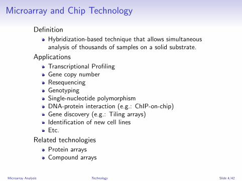
Microarray and Chip Technology

Definition

Hybridization-based technique that allows simultaneousanalysis of thousands of samples on a solid substrate.

Applications

Transcriptional ProfilingGene copy numberResequencingGenotypingSingle-nucleotide polymorphismDNA-protein interaction (e.g.: ChIP-on-chip)Gene discovery (e.g.: Tiling arrays)Identification of new cell linesEtc.

Related technologies

Protein arraysCompound arrays

Microarray Analysis Technology Slide 4/42

Why Microarrays?

Simultaneous analysis of thousands of genes

Discovery of gene functions

Genome-wide network analysis

Analysis of mutants and transgenics

Identification of drug targets

Causal understanding of diseases

Clinical studies and field trials

Microarray Analysis Technology Slide 5/42

Different Types of Microarrays

Single channel approaches

Affymetrix gene chipsMacroarrays

Multiple channel approaches

Dual color (cDNA) microarrays

Specialty approaches

Bead arrays: Lynx, Illumina, ...PCR-based profiling: CuraGen, ...

Microarray Analysis Technology Slide 6/42

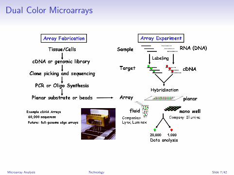
Dual Color Microarrays

Microarray Analysis Technology Slide 7/42

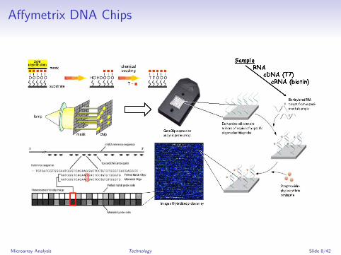
Affymetrix DNA Chips

Microarray Analysis Technology Slide 8/42

Outline

Technology

Challenges

Data Analysis

Data Depositories

R and BioConductor

Homework Assignment

Microarray Analysis Challenges Slide 9/42

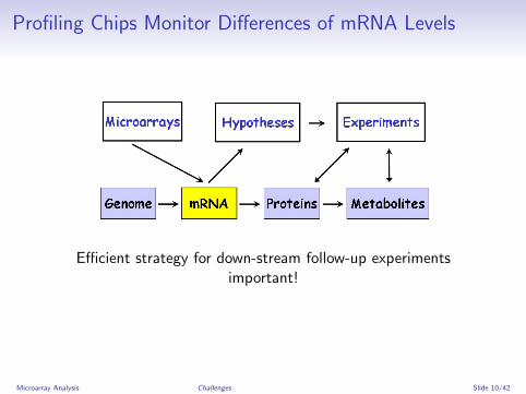
Profiling Chips Monitor Differences of mRNA Levels

Efficient strategy for down-stream follow-up experimentsimportant!

Microarray Analysis Challenges Slide 10/42

Strategies to Validate Array Hits

Real-time PCR, Northern, etc.

Transgenic tests

Knockout plants and/or activation tagged lines

Protein profiling

Metabolic profiling

Other tests: in situ hybs, biochemical and physiological tests

Integration with sequence, proteomics and metabolicdatabases

Microarray Analysis Challenges Slide 11/42

Sources of Variation in Transcriptional ProfilingExperiments

Every step in transcriptional profiling experiments cancontribute to the inherent ’noise’ of array data.

Variations in biosamples, RNA quality and target labeling arenormally the biggest noise introducing steps in arrayexperiments.

Careful experimental design and initial calibration experimentscan minimize those challenges.

Microarray Analysis Challenges Slide 12/42

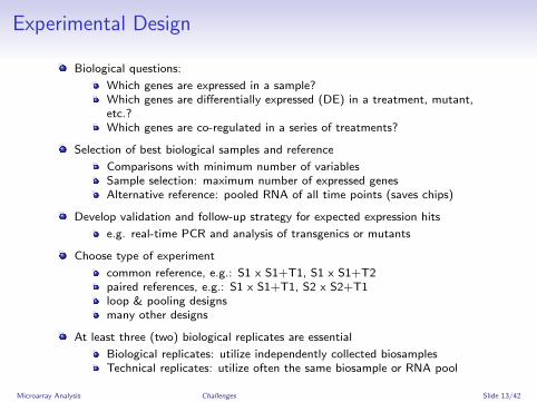
Experimental Design

Biological questions:

Which genes are expressed in a sample?Which genes are differentially expressed (DE) in a treatment, mutant,etc.?Which genes are co-regulated in a series of treatments?

Selection of best biological samples and reference

Comparisons with minimum number of variablesSample selection: maximum number of expressed genesAlternative reference: pooled RNA of all time points (saves chips)

Develop validation and follow-up strategy for expected expression hits

e.g. real-time PCR and analysis of transgenics or mutants

Choose type of experiment

common reference, e.g.: S1 x S1+T1, S1 x S1+T2paired references, e.g.: S1 x S1+T1, S2 x S2+T1loop & pooling designsmany other designs

At least three (two) biological replicates are essential

Biological replicates: utilize independently collected biosamplesTechnical replicates: utilize often the same biosample or RNA pool

Microarray Analysis Challenges Slide 13/42

Outline

Technology

Challenges

Data Analysis

Data Depositories

R and BioConductor

Homework Assignment

Microarray Analysis Data Analysis Slide 14/42

Basic Data Analysis Steps

Image Processing: transform feature and background pixelinto intensity values

Transformations

Removal of flagged values (optional)Detection limit (optional)Background subtractionTaking logarithms

Normalization

Identify EGs and DEGs

Which genes are expressed?Which genes are differentially expressed?

Cluster analysis (time series)

Which genes have similar expression profiles?

Promoter analysis

Integration with functional information: pathways, etc.

Microarray Analysis Data Analysis Slide 15/42

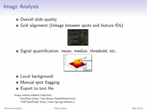
Image Analysis

Overall slide quality

Grid alignment (linkage between spots and feature IDs)

Signal quantification: mean, median, threshold, etc.

Local background

Manual spot flagging

Export to text file

Image analysis software (selection)

ScanAlyze (http://rana.lbl.gov/EisenSoftware.htm)

TIGR SpotFinder (http://www.tigr.org/software/)

Microarray Analysis Data Analysis Slide 16/42

Background Correction

Filtering (optional)

Intensities below detection limitNegative intensitiesSpacial quality issues

Background correction

BG consists of non-specific hybridization and backgroundfluorescenceIf BG is higher than signal: (1) remove values, (2) set signal tolowest measured intensity, (3) many other approachesBG subtraction

Local backgroundGlobal backgroundNo background subtraction

Background subtraction can cause ratio inflation, thereforebackground corrected intensities below threshold are often setto threshold or similar value.

Microarray Analysis Data Analysis Slide 17/42

Normalization

Normalization is the process of balancing the intensities of thechannels to account for variations in labeling and hybridizationefficiencies. To achieve this, various adjustment strategies are usedto force the distribution of all ratios to have a median (mean) of 1or the log-ratios to have a median (mean) of 0.

Microarray Analysis Data Analysis Slide 18/42

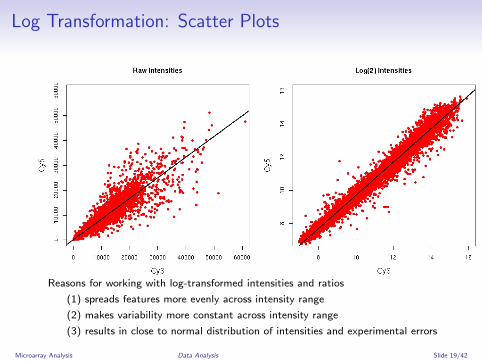
Log Transformation: Scatter Plots

Reasons for working with log-transformed intensities and ratios

(1) spreads features more evenly across intensity range

(2) makes variability more constant across intensity range

(3) results in close to normal distribution of intensities and experimental errors

Microarray Analysis Data Analysis Slide 19/42

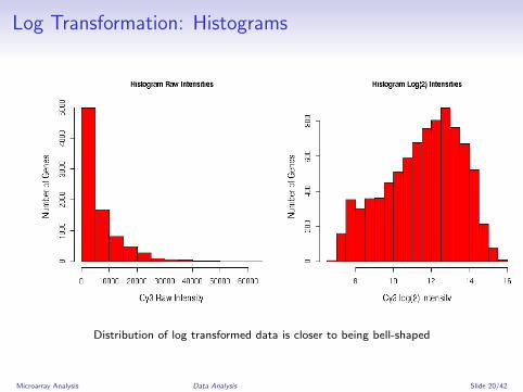
Log Transformation: Histograms

Distribution of log transformed data is closer to being bell-shaped

Microarray Analysis Data Analysis Slide 20/42

Normalization If Large Fraction of Genes IS DE

Minimize normalization requirements (dynamic range limits)

Pre-scanning: hybridize equal amounts of label

During scanning: balance average intensities through laserpower and PMP adjustments

Normalization if large fraction of genes is DE

Spike-in controls

Housekeeping controls

Determine constant feature set

Microarray Analysis Data Analysis Slide 21/42

Normalization If Large Fraction of Genes IS NOT DE

Global Within-Array Normalization

Multiply one channels with normalization factor⇒ Ch2 x mCh1/mCh2 (treats both channels differently)

Linear regression fit of log2(Ch2) against log2(Ch1)⇒ adjust Ch1 with fitted values (treats both channelsdifferently)

Linear regression fit of log2(ratios) against avg log2(int)⇒ subtract fitted value from raw log ratios (treats bothchannels equally)

Non-linear regression fit of log2(ratios) against avg log2(int)Most commonly used: Loess (locally weighted polynomial)regression joins local regressions with overlapping windows tosmooth curve⇒ subtract fitted value on Loess regression from raw logratios (treats both channels equally)

Microarray Analysis Data Analysis Slide 22/42

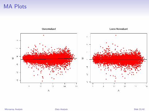
MA Plots

Microarray Analysis Data Analysis Slide 23/42

Normalization If Large Fraction of Genes IS NOT DE

Spacial Within-Array Normalization

All of the above methods can be used to correct for spacialbias on the array. Examples:

Block or Print Tip Loess

2D Loess Regression

Microarray Analysis Data Analysis Slide 24/42

Normalization If Large Fraction of Genes IS NOT DE

Between-Array NormalizationTo compare ratios between dual-color arrays or intensitiesbetween single-color arrays

Scaling⇒ log(rat) - mean log(rat) or log(int) - mean log(int)⇒ Result: mean = 0

Centering (z-value)⇒ [rat - mean(rat)] / [STD] or [int - mean(int)] / [STD]⇒ Result: mean = 0, STD = 1

Distribution Normalization (apply to group of arrays!)⇒ (1) Generate centered data, (2) sort each array byintensities, (3) calculate mean for sorted values across arrays,(4) replace sorted array intensities by corresponding meanvalues, (5) sort data back to original order⇒ Result: mean = 0, STD = 1, identical distribution betweenarrays

Microarray Analysis Data Analysis Slide 25/42

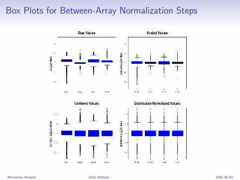
Box Plots for Between-Array Normalization Steps

Microarray Analysis Data Analysis Slide 26/42

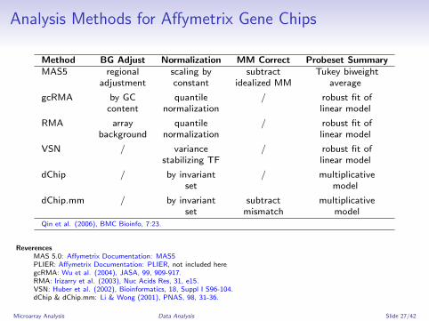
Analysis Methods for Affymetrix Gene Chips

Method BG Adjust Normalization MM Correct Probeset SummaryMAS5 regional scaling by subtract Tukey biweight

adjustment constant idealized MM average

gcRMA by GC quantile / robust fit ofcontent normalization linear model

RMA array quantile / robust fit ofbackground normalization linear model

VSN / variance / robust fit ofstabilizing TF linear model

dChip / by invariant / multiplicativeset model

dChip.mm / by invariant subtract multiplicativeset mismatch model

Qin et al. (2006), BMC Bioinfo, 7:23.

ReverencesMAS 5.0: Affymetrix Documentation: MAS5PLIER: Affymetrix Documentation: PLIER, not included heregcRMA: Wu et al. (2004), JASA, 99, 909-917.RMA: Irizarry et al. (2003), Nuc Acids Res, 31, e15.VSN: Huber et al. (2002), Bioinformatics, 18, Suppl I S96-104.dChip & dChip.mm: Li & Wong (2001), PNAS, 98, 31-36.

Microarray Analysis Data Analysis Slide 27/42

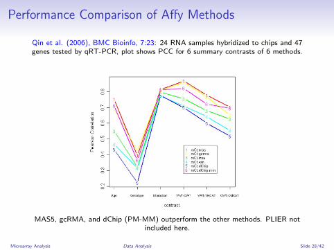
Performance Comparison of Affy Methods

Qin et al. (2006), BMC Bioinfo, 7:23: 24 RNA samples hybridized to chips and 47genes tested by qRT-PCR, plot shows PCC for 6 summary contrasts of 6 methods.

MAS5, gcRMA, and dChip (PM-MM) outperform the other methods. PLIER notincluded here.

Microarray Analysis Data Analysis Slide 28/42

Analysis of Differentially Expressed Genes

Advantages of statistical test over fold change threshold forselecting DE genes

Incorporates variation between measurementsEstimate for error rateDetection of minor changesRanking of DE genes

Approaches

Parametric test: t-testNon-parametric tests: Wilcoxon sign-rank/rank-sum testsBootstrap analysis (boot package)Significance Analysis of Microarrays (SAM)Linear Models of Microarrays (LIMMA)Rank ProductANOVA and MANOVA (R/maanova)

Multiplicity of testing: p-value adjustments

Methods: fdr, bonferroni, etc.

Microarray Analysis Data Analysis Slide 29/42

Outline

Technology

Challenges

Data Analysis

Data Depositories

R and BioConductor

Homework Assignment

Microarray Analysis Data Depositories Slide 30/42

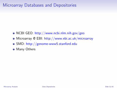
Microarray Databases and Depositories

NCBI GEO: http://www.ncbi.nlm.nih.gov/geo

Microarray @ EBI: http://www.ebi.ac.uk/microarray

SMD: http://genome-www5.stanford.edu

Many Others

Microarray Analysis Data Depositories Slide 31/42

Outline

Technology

Challenges

Data Analysis

Data Depositories

R and BioConductor

Homework Assignment

Microarray Analysis R and BioConductor Slide 32/42

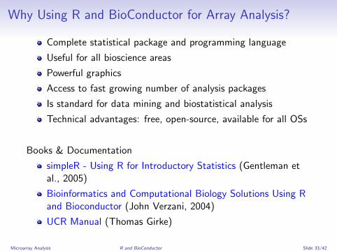
Why Using R and BioConductor for Array Analysis?

Complete statistical package and programming language

Useful for all bioscience areas

Powerful graphics

Access to fast growing number of analysis packages

Is standard for data mining and biostatistical analysis

Technical advantages: free, open-source, available for all OSs

Books & Documentation

simpleR - Using R for Introductory Statistics (Gentleman etal., 2005)

Bioinformatics and Computational Biology Solutions Using Rand Bioconductor (John Verzani, 2004)

UCR Manual (Thomas Girke)

Microarray Analysis R and BioConductor Slide 33/42

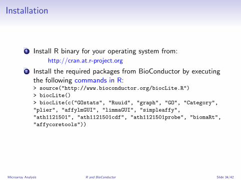
Installation

1 Install R binary for your operating system from:

http://cran.at.r-project.org

2 Install the required packages from BioConductor by executingthe following commands in R:> source("http://www.bioconductor.org/biocLite.R")

> biocLite()

> biocLite(c("GOstats", "Ruuid", "graph", "GO", "Category",

"plier", "affylmGUI", "limmaGUI", "simpleaffy",

"ath1121501", "ath1121501cdf", "ath1121501probe", "biomaRt",

"affycoretools"))

Microarray Analysis R and BioConductor Slide 34/42

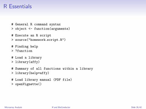
R Essentials

# General R command syntax

> object <- function(arguments)

# Execute an R script

> source("homework script.R")

# Finding help

> ?function

# Load a library

> library(affy)

# Summary of all functions within a library

> library(help=affy)

# Load library manual (PDF file)

> openVignette()

Microarray Analysis R and BioConductor Slide 35/42

Outline

Technology

Challenges

Data Analysis

Data Depositories

R and BioConductor

Homework Assignment

Microarray Analysis Homework Assignment Slide 36/42

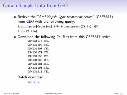
Obtain Sample Data from GEO

Retieve the ”Arabidopsis light treatment series” (GSE5617)from GEO with the following query:Arabidopsis[Organism] AND Atgenexpress[Title] AND

light[Title]

Download the following Cel files from this GSE5617 series:GSM131177.CEL

GSM131192.CEL

GSM131207.CEL

GSM131179.CEL

GSM131193.CEL

GSM131209.CEL

GSM131181.CEL

GSM131195.CEL

GSM131211.CEL

Batch download:GEO CEL.zip

Microarray Analysis Homework Assignment Slide 37/42

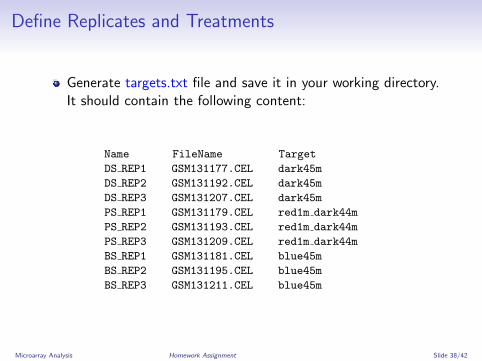
Define Replicates and Treatments

Generate targets.txt file and save it in your working directory.It should contain the following content:

Name FileName Target

DS REP1 GSM131177.CEL dark45m

DS REP2 GSM131192.CEL dark45m

DS REP3 GSM131207.CEL dark45m

PS REP1 GSM131179.CEL red1m dark44m

PS REP2 GSM131193.CEL red1m dark44m

PS REP3 GSM131209.CEL red1m dark44m

BS REP1 GSM131181.CEL blue45m

BS REP2 GSM131195.CEL blue45m

BS REP3 GSM131211.CEL blue45m

Microarray Analysis Homework Assignment Slide 38/42

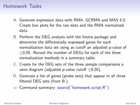
Homework Tasks

A. Generate expression data with RMA, GCRMA and MAS 5.0.Create box plots for the raw data and the RMA normalizeddata.

B. Perform the DEG analysis with the limma package anddetermine the differentially expressed genes for eachnormalization data set using as cutoff an adjusted p-value of≤0.05. Record the number of DEGs for each of the threenormalization methods in a summary table.

C. Create for the DEG sets of the three sample comparisons avenn diagram (adjusted p-value cutoff ≤0.05).

D. Generate a list of genes (probe sets) that appear in all threefiltered DEG sets (from B.).

⇒ Command summary: source(”homework script.R”)

Microarray Analysis Homework Assignment Slide 39/42

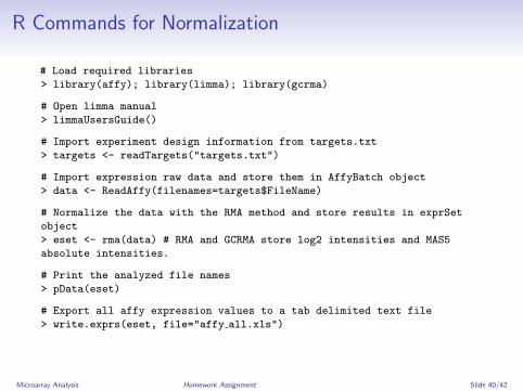
R Commands for Normalization

# Load required libraries

> library(affy); library(limma); library(gcrma)

# Open limma manual

> limmaUsersGuide()

# Import experiment design information from targets.txt

> targets <- readTargets("targets.txt")

# Import expression raw data and store them in AffyBatch object

> data <- ReadAffy(filenames=targets$FileName)

# Normalize the data with the RMA method and store results in exprSet

object

> eset <- rma(data) # RMA and GCRMA store log2 intensities and MAS5

absolute intensities.

# Print the analyzed file names

> pData(eset)

# Export all affy expression values to a tab delimited text file

> write.exprs(eset, file="affy all.xls")

Microarray Analysis Homework Assignment Slide 40/42

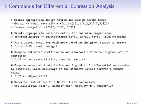
R Commands for Differential Expression Analysis

# Create appropriate design matrix and assign column names

> design <- model.matrix(∼ -1+factor(c(1,1,1,2,2,2,3,3,3)));

colnames(design) <- c("S1", "S2", "S3")

# Create appropriate contrast matrix for pairwise comparisons

> contrast.matrix <- makeContrasts(S2-S1, S3-S2, S3-S1, levels=design)

# Fit a linear model for each gene based on the given series of arrays

> fit <- lmFit(eset, design)

# Compute estimated coefficients and standard errors for a given set of

contrasts

> fit2 <- contrasts.fit(fit, contrast.matrix)

# Compute moderated t-statistics and log-odds of differential expression

by empirical Bayes shrinkage of the standard errors towards a common

value

> fit2 <- eBayes(fit2)

# Generate list of top 10 DEGs for first comparison

> topTable(fit2, coef=1, adjust="fdr", sort.by="B", number=10)

Microarray Analysis Homework Assignment Slide 41/42

Online Manual

Continue on online manual.

Microarray Analysis Homework Assignment Slide 42/42