microcom model gtx-2.0 satellite transmitter and data ...€¦ · data logger configuration utility...
TRANSCRIPT
Microcom Model GTX-2.0 Satellite Transmitter
and Data Logger
Configuration Utility Operation and Maintenance
Version 2.20 Release 1
Microcom Design, Inc.
10948 Beaver Dam Road, Suite C Hunt Valley, MD 21030

Microcom GTX-2.0 O&M Manual V2.20/R1
Microcom Design, Inc. ii
Table of Contents
1. Introduction.......................................................................................................................................... 1 1.1. Manual Organization ........................................................................................................................ 1 1.1.1. GTX Configuration and Upgrade Utilities ..................................................................................... 1 1.2. Theory of Operation ......................................................................................................................... 2 1.2.1. Main Microcontroller...................................................................................................................... 2 1.2.2. Time Keeping Microcontroller ....................................................................................................... 2 1.2.3. GTX-2.0 Operational Overview..................................................................................................... 3 1.2.3.1. Time Management..................................................................................................................... 3 1.2.3.1.1. Data Transmission Scheduler ................................................................................................. 3 1.2.3.1.2. Real-Time Clock Update and TCXO Calibration Scheduler ................................................... 4 1.2.3.1.3. Data Collection (SDI-12, Internal Sensors, and Equation) Scheduler .................................... 4 1.2.3.2. Data/Memory Storage ............................................................................................................... 4 1.2.3.2.1. Satellite Transmit Buffers ........................................................................................................ 4 1.2.3.2.1.1. Timed Transmit Buffer ......................................................................................................... 5 1.2.3.2.1.2. Random Transmit Buffer...................................................................................................... 5 1.2.3.2.2. Data/Event Log........................................................................................................................ 6 1.2.3.2.3. Configuration Memory ............................................................................................................. 6 1.2.3.2.4. Program/Firmware Memory..................................................................................................... 7 1.2.3.3. Satellite Message Transmission Messages .............................................................................. 7 1.2.3.3.1. GOES ASCII and Pseudo-Binary Transmit Buffer Formatting................................................ 7 1.2.3.3.2. GOES Binary Buffer Formatting .............................................................................................. 8 1.2.3.4. RF Transmitter Control .............................................................................................................. 8 1.2.3.4.1. Battery Voltage Monitor ........................................................................................................... 8 1.2.3.4.2. Transmitter Power Control ...................................................................................................... 9 1.2.3.4.3. Channel Selection Synthesizer ............................................................................................... 9 1.2.3.4.4. Forward and Reverse Power Monitor ..................................................................................... 9 1.2.3.4.5. Symbol Timing, Data Modulation, and AGC ........................................................................... 9 1.2.3.5. Serial Port Interface................................................................................................................... 9 1.2.3.6. SDI-12 Interface ...................................................................................................................... 10 1.2.3.7. Internal Sensors (Temperature, Tipping Bucket, Battery Voltage).......................................... 10 1.2.3.8. Internal Sensors (Equation Processor) ................................................................................... 10 1.2.3.9. Min, Max, Average (MMA) Processor ..................................................................................... 10 1.2.3.10. TKM Real-Time Clock and BBU-RTC ..................................................................................... 11 1.2.3.10.1. TCXO Temperature Sensor .................................................................................................. 11 1.2.3.10.2. Temperature Monitor Function .............................................................................................. 11 1.2.3.11. Main Microcontroller Wake Up ................................................................................................ 12 1.2.3.11.1. Alarm Clock Function ............................................................................................................ 12 1.2.3.11.2. Serial Port Activity ................................................................................................................. 12 1.2.3.11.3. Push-Button Wakeup ............................................................................................................ 13 1.2.3.12. GPS Receiver and Interface.................................................................................................... 13 1.2.3.12.1. Clock Set and Synchronization to UTC................................................................................. 13 1.2.3.12.2. TCXO Frequency Calibration ................................................................................................ 14 1.2.3.12.3. Lat/Long Position................................................................................................................... 14 1.2.3.13. Failsafe Transmit Monitor ........................................................................................................ 14 1.2.3.14. Push-Button/LED Interface...................................................................................................... 15
2. GTX Hardware Set Up ...................................................................................................................... 16 2.1. Connector Information.................................................................................................................... 16 2.1.1. Main Power Connections............................................................................................................ 16 2.1.2. RF Output Connections .............................................................................................................. 16 2.1.3. Tipping Bucket and Custom I/O Connections............................................................................. 17 2.1.4. GPS Antenna Connections......................................................................................................... 17 2.1.5. RS-232 Serial Port Connections................................................................................................. 18 2.1.6. SDI-12 Connections.................................................................................................................... 18

Microcom GTX-2.0 O&M Manual V2.20/R1
Microcom Design, Inc. iii
2.2. Failsafe Reset Push-Button and LED Indicators ........................................................................... 19 2.3. Site Cable Connections.................................................................................................................. 19 2.4. Power Supply, Battery and Power Consumption........................................................................... 19 2.5. Antenna Selections and Mounting ................................................................................................. 19
3. GTX-2.0 Basic Operation and Configuration..................................................................................... 21 3.1. Terminal Interface .......................................................................................................................... 21 3.1.1. Typical Command Usage ........................................................................................................... 21 3.2. Configuration Utility Overview........................................................................................................ 23 3.2.1. Create/Open A Setup Template ................................................................................................. 24 3.2.2. Configure GTX From A Template ............................................................................................... 26 3.2.3. Monitor/Inspect GTX................................................................................................................... 27 3.2.4. Configure/Control/Deploy GTX................................................................................................... 28 3.2.5. Configuration and Template Files............................................................................................... 29 3.3. Terminal versus Configuration Utility ............................................................................................. 30 3.4. Enabled versus Disabled Operation .............................................................................................. 31 3.4.1. Transmitter versus Data Logger Functions – Setting the GTX Operation Mode........................ 31 3.4.2. Configuring the GTX to Power Up Enabled................................................................................ 32 3.5. GPS Time Sync and TCXO Calibration Settings ........................................................................... 33
4. GTX Operation with GOES ............................................................................................................... 35 4.1. GOES DCS Description ................................................................................................................. 35 4.2. Set Up for Use with Self-Timed Operation..................................................................................... 37 4.2.1. Terminal Configuration for GOES Self-Timed Operation ........................................................... 37 4.2.2. Utility Configuration for Self-Timed Operation ............................................................................ 38 4.3. Set Up for Use with Random Operation......................................................................................... 39 4.3.1. Terminal Configuration for Random Operation........................................................................... 39 4.3.2. Utility Configuration for Random Operation................................................................................ 40 4.4. Timed and Random Operation Flags............................................................................................. 41 4.4.1. Common Operation Flags........................................................................................................... 41 4.4.2. Timed Only Operation Flags....................................................................................................... 42 4.4.2.1. Center Transmission in Window.............................................................................................. 42 4.4.2.2. Timed Buffer Control Flags...................................................................................................... 42
5. Soft Configuration.............................................................................................................................. 43 5.1. Soft Configuration Allocation and Memory Usage ......................................................................... 43
6. Data Collection .................................................................................................................................. 45 6.1. Basic Operation.............................................................................................................................. 45 6.1.1. RS-232 Data Collection Using an External Data System........................................................... 45 6.1.2. Sensor Data Collection ............................................................................................................... 45 6.1.2.1. Internal Sensors ...................................................................................................................... 46 6.1.2.1.1. Temperature Sensor ............................................................................................................. 47 6.1.2.1.2. Tipping Bucket Counter......................................................................................................... 48 6.1.2.1.2.1. Tipping Bucket Scaling ...................................................................................................... 48 6.1.2.1.2.2. Tipping Bucket Rollover..................................................................................................... 48 6.1.2.1.2.3. Tipping Bucket Auto Clear ................................................................................................. 48 6.1.2.1.3. Battery Voltage...................................................................................................................... 49 6.1.2.1.4. Equation Internal Sensors ..................................................................................................... 49 6.1.2.1.5. Clock Internal Sensors .......................................................................................................... 51 6.1.2.1.6. Testing the Internal Sensors ................................................................................................. 52 6.1.2.2. SDI-12 Data Collection ............................................................................................................ 53 6.1.3. SDI-12 Power Control ................................................................................................................. 55 6.1.4. Sensor Data Logging .................................................................................................................. 57 6.1.5. Sensor Labeling .......................................................................................................................... 58
7. Equation Processor ........................................................................................................................... 60 7.1. Equation Basics ............................................................................................................................. 60
Microcom GTX-2.0 O&M Manual V2.20/R1
Microcom Design, Inc. iv
7.1.1. Equation Operators..................................................................................................................... 60 7.1.2. Equation Constants..................................................................................................................... 62 7.1.2.1. Inline Constants ....................................................................................................................... 62 7.1.2.2. Configuration Constants .......................................................................................................... 62 7.1.3. Equation Variables...................................................................................................................... 64 7.1.3.1. Sensor Variable Standard Designations ................................................................................. 64 7.1.3.2. Sensor Label Variable ............................................................................................................. 64 7.1.3.3. Configuration Constant Labels ................................................................................................ 64 7.1.3.4. MMA Processor Variables ....................................................................................................... 65 7.1.3.4.1. MMA Variables Standard Designations ................................................................................ 65 7.1.3.4.2. MMA Variables Pseudo Functions ........................................................................................ 66 7.1.4. Equation Arithmetic Functions .................................................................................................... 66 7.2. Format Specifiers for Equations..................................................................................................... 67 7.3. Entering and Editing Equations using the Configuration Utility ..................................................... 68 7.4. If-Construct (?) for Equations......................................................................................................... 69 7.5. Equation Initial Conditions ............................................................................................................. 71 7.5.1. Initial Sensor, Variable, and Equation Values ............................................................................ 71 7.5.2. Initialization Equations ................................................................................................................ 71 7.6. Default Labels, Standard Designators, Functions ......................................................................... 72
8. Min, Max, Average (MMA) Processor ............................................................................................... 73 8.1. MMA Basics and Configuration Utility Definition............................................................................ 73 8.2. MMA Vector Average ..................................................................................................................... 75
9. Formatting Transmission Buffers ...................................................................................................... 77 9.1. Header Parameters........................................................................................................................ 78 9.2. Sensor Parameters ........................................................................................................................ 79 9.3. ASCII Versus Pseudo-Binary Formatting....................................................................................... 80 9.3.1. Rounding versus Truncating for Transmission Buffers............................................................... 82 9.4. Data Buffer Configuration............................................................................................................... 83 9.4.1. Timed Data Buffer Configuration Example – ASCII Formatting ................................................. 83 9.4.1.1. Timed Data Buffer Configuration Example – ASCII Flags ...................................................... 84 9.4.1.1.1. Timed Data Buffer Configuration Example – Labels ............................................................. 85 9.4.1.1.2. Timed Data Buffer Configuration Example – Record Terminators........................................ 85 9.4.1.1.3. Timed Data Buffer Configuration Example – Leading Zero .................................................. 86 9.4.1.2. Timed Data Buffer Configuration Example – Summary .......................................................... 86 9.4.2. Random Data Buffer Configuration Example – Pseudo-Binary Formatting ............................... 87 9.4.3. Including Min, Max, and Average Data in Transmission Buffers................................................ 90 9.5. Random Report Triggering ............................................................................................................ 92 9.6. Random Report Triggers for Sensor Logging Only ....................................................................... 95 9.7. Slash Fill Option for Transmission Buffers..................................................................................... 96 9.8. Text Transmit Parameter ............................................................................................................... 98
10. Retrieving Logged Data................................................................................................................... 100 10.1. Log Retrieval Using the Configuration Utility ............................................................................... 100 10.2. Retrieving Selected Entries – Filtered Log Retrieval ................................................................... 102 10.3. CSV Log Dump Format................................................................................................................ 103 10.4. Log Retrieval Using the Terminal Interface.................................................................................. 103 10.5. Auto Log Monitor.......................................................................................................................... 105 10.6. Log Dump Timing – Terminal versus Utility ................................................................................. 105 10.7. Data Graphing.............................................................................................................................. 106 10.8. Logged Events Summary............................................................................................................. 108
11. RS-232 Serial Port Interface Command Reference........................................................................ 110 11.1. RS-232 Command Protocol ......................................................................................................... 110 11.1.1. RS-232 Interface Protocol ........................................................................................................ 110 11.1.2. RS-232 Hardware Interface ...................................................................................................... 110 11.1.3. RS-232 Command Format........................................................................................................ 110
Microcom GTX-2.0 O&M Manual V2.20/R1
Microcom Design, Inc. v
11.1.4. RS-232 Access Rights .............................................................................................................. 111 11.1.5. Password Protection for Configuration Commands.................................................................. 111 11.2. Satellite Transmission Configuration Commands........................................................................ 112 11.2.1. Platform ID (PID=xxxxxxxx) [dtx] .............................................................................................. 112 11.2.2. GTX Operation Mode (GTX=x) [dtx] ......................................................................................... 112 11.2.3. Timed Transmit Channel (TCH=ccc,bbbb) [dtx] ....................................................................... 112 11.2.4. Timed Transmit Interval (TTI=dd:hh:mm:ss) [dtx]..................................................................... 113 11.2.5. First Transmission Time (FTT=hh:mm:ss) [dtx]........................................................................ 113 11.2.6. Timed Window Length (TWL=xxx) [dtx].................................................................................... 113 11.2.7. Timed Operation Flags (TOF=xx) [dtx] ..................................................................................... 113 11.2.8. Timed Preamble (TPR=xxxxx) [dtx].......................................................................................... 113 11.2.9. Timed Data Format (TDF=xxxxxx) [dtx].................................................................................... 114 11.2.10. Timed Data Source (TDS=xxxxxx) [dtx] ................................................................................... 114 11.2.11. Timed Data Order (TDO=xxxxxx) [dtx] ..................................................................................... 114 11.2.12. Random Transmit Channel (RCH=ccc,bbbb) [dtx] ................................................................... 114 11.2.13. Random Transmit Interval (RIN=xxx) [dtx] ............................................................................... 114 11.2.14. Randomization Percent (RPC=pp) [dtx] ................................................................................... 114 11.2.15. Random Repeat Count (RRC=xx) [dtx] .................................................................................... 115 11.2.16. Random Data Format (RDF=xxxxxx) [dtx]................................................................................ 115 11.2.17. Random Data Source (RDS=xxxxxx) [dtx] ............................................................................... 115 11.2.18. Random Data Order (RDO=xxxxxx) [dtx] ................................................................................. 115 11.2.19. Random Operation Flags (ROF=xx) [dtx] ................................................................................. 116 11.3. General Transmitter Configuration Commands ........................................................................... 116 11.3.1. Transmit Power (TXP=a.a,[b.b]) [dtx] ....................................................................................... 116 11.3.2. Time (TIM=hh:mm:ss) [dtx]....................................................................................................... 116 11.3.3. Date (DAT=mm/dd/yyyy) [dtx]................................................................................................... 117 11.3.4. Time Correct (TIC) [all] ............................................................................................................. 117 11.3.5. Time Zone Offset (TZN) [dtx].................................................................................................... 117 11.3.6. UTC Correction (UTC) [all] ....................................................................................................... 117 11.3.7. Invalid Replace Character (IRC=c) [dtx] ................................................................................... 117 11.3.8. Slash Fill (SFL=b) [dtx] ............................................................................................................. 118 11.3.9. Power Up Enabled (PUE=b) [dtx] ............................................................................................. 118 11.4. RS-232 Transmit Data Storage Commands ................................................................................ 118 11.4.1. Literal Character Designator, ‘/’ ................................................................................................ 118 11.4.2. Timed Data Buffer Load (TDT=xxx…) [etx] .............................................................................. 119 11.4.3. Timed Buffer Size (TBS?) [all] .................................................................................................. 119 11.4.4. Clear Timed Buffer (CTB) [all] .................................................................................................. 119 11.4.5. Timed Buffer Dump (TBD) [all] ................................................................................................. 119 11.4.6. Random Data Buffer Load (RDT=xxx…) [etx] .......................................................................... 120 11.4.7. Random Buffer Size (RBS?) [all] .............................................................................................. 120 11.4.8. Clear Random Buffer (CRB) [all] .............................................................................................. 121 11.4.9. Random Buffer Dump (RBD) [all] ............................................................................................. 121 11.4.10. Random Buffer Transmissions Remaining (RBT) [all] .............................................................. 121 11.5. Data Collection Setup and Test Commands................................................................................ 121 11.5.1. SDI-12 Data Collection Setup and Test Commands ................................................................ 121 11.5.1.1. Number of SDI-12 Sensors (SSN=xx) [dtx] ........................................................................... 122 11.5.1.2. SDI-12 Command Basics ...................................................................................................... 122 11.5.1.3. SDI-12 Sensor Definition (SSX=a,m,p,rate,offset,<log>) [dtx] .............................................. 123 11.5.1.4. SDI-12 Sensor Label (SLX=xxxx) [dtx].................................................................................. 125 11.5.1.5. Next SDI-12 Sample (SMX) [all] ............................................................................................ 126 11.5.1.6. SDI-12 Test Command (SDI) [all].......................................................................................... 126 11.5.1.7. SDI-12 Timeout Setting (STO=xx) [all] .................................................................................. 128 11.5.2. SDI-12 Power Control Commands ........................................................................................... 128 11.5.2.1. SDI-12 Power Control (SPC) [all] .......................................................................................... 128 11.5.2.2. SDI-12 Power Mode (SPM) [dtx] ........................................................................................... 129 11.5.2.3. SDI-12 Power Table Entry (SPX) [dtx] .................................................................................. 129

Microcom GTX-2.0 O&M Manual V2.20/R1
Microcom Design, Inc. vi
11.5.3. Internal Sensor Data Collection Setup and Test Commands................................................... 130 11.5.3.1. Number of Internal Sensors (ISN=xx) [dtx]............................................................................ 130 11.5.3.2. Internal Sensor Command Basics ......................................................................................... 130 11.5.3.3. Internal Sensor Definition (ISX=t,rate,offset,<log>) [dtx]....................................................... 131 11.5.3.4. Internal Sensor Label (ILX=xxxx) [dtx] .................................................................................. 133 11.5.3.5. Next Internal Sensor Sample (IMX) [all] ................................................................................ 133 11.5.3.6. Internal Sensor Test (IST) [all]............................................................................................... 134 11.5.3.7. TCXO Temperature (TOT) [all] – Internal Temperature........................................................ 134 11.5.3.8. Tipping Bucket Count (TBC) [all] ........................................................................................... 134 11.5.3.9. Tipping Bucket Value (TBV) [all] ........................................................................................... 135 11.5.3.10. Tipping Bucket Multiplier (TBM=xxx) [dtx] ............................................................................. 135 11.5.3.11. Tipping Bucket Rollover (TBR=xxxxx) [dtx] ........................................................................... 135 11.5.3.12. Tipping Bucket Auto Clear (TBA=xxx) [dtx] ........................................................................... 135 11.6. Equation and Min, Max, Average (MMA) Commands ................................................................. 136 11.6.1. Equation Definition (EQN) [dtx]................................................................................................. 136 11.6.2. Equation Test (EQT) [dtx] ......................................................................................................... 137 11.6.3. Equation Constants................................................................................................................... 138 11.6.3.1. Number of Equation Constants (EKN=xx) [dtx] ..................................................................... 138 11.6.3.2. Equation Constant Value (EKV) [all] ..................................................................................... 138 11.6.3.3. Equation Constant Label (EKL) [dtx] ..................................................................................... 139 11.6.4. Equation Variable (EQV) [all] .................................................................................................... 139 11.6.5. Number of Min, Max, Average Processors (MMN=xx) [dtx] ..................................................... 139 11.6.6. Min, Max, Average Definition (MMA=sensor,rate,offset,<flags>) [dtx] ..................................... 139 11.7. Data Transmission Storage Setup Commands ........................................................................... 141 11.7.1. Number of Timed Buffer Parameters (TPN=xxx) [dtx].............................................................. 141 11.7.2. Number of Random Buffer Parameters (RPN) [dtx] ................................................................. 141 11.7.3. Timed and Random Data Parameter Definition (TDP & RDP) [dtx] ......................................... 142 11.7.3.1. Header Data Parameters....................................................................................................... 145 11.7.3.1.1. Platform Identification String (PIS) [dtx] .............................................................................. 146 11.7.3.1.2. Pseudo Binary Character 1 and 2 (PB1 and PB2) [dtx] ...................................................... 146 11.7.3.2. Sensor Data Parameters ....................................................................................................... 146 11.7.3.3. Appending Min, Max, and Average Data to Sensor Data Parameters.................................. 148 11.7.3.4. Text Field Parameters ........................................................................................................... 149 11.7.4. Number of Random Triggers (RTN) [dtx].................................................................................. 149 11.7.5. Random Report Trigger Definition (RRT) [dtx] ......................................................................... 149 11.8. Time Sync and Oscillator Calibration Configuration .................................................................... 151 11.8.1. GPS Time Sync Interval (GTS=ttt) [dtx].................................................................................... 151 11.8.2. GPS TCXO Calibration (GTC=dd) [dtx] .................................................................................... 152 11.8.3. GPS OCXO Calibration (GOC=dd) [dtx]................................................................................... 152 11.8.4. GPS Sync/Calibration Timeout (GTO=to) [dtx]......................................................................... 152 11.8.5. GPS Log Sync/Calibration (GLG=f) [dtx] .................................................................................. 152 11.9. General Configuration Commands .............................................................................................. 152 11.9.1. RS-232 Command Active Time (CAT) [all] ............................................................................... 152 11.9.2. Configuration Save (CFS) [dtx]................................................................................................. 152 11.9.3. Configuration Restore (CFR) [dtx] ............................................................................................ 152 11.9.4. Configuration Default (ConfigDefault) [dtx] ............................................................................... 153 11.9.5. Configuration Verify (CFV) [all] ................................................................................................. 153 11.9.6. Configuration Change Begin (CFB) [dtx] .................................................................................. 153 11.9.7. Configuration Enable (CFE) [dtx].............................................................................................. 153 11.9.8. Configuration Password (CPW) [dtx] ........................................................................................ 153 11.9.9. Configuration Memory Available (CMA) [dtx] ........................................................................... 154 11.10. Status and Other Commands ...................................................................................................... 154 11.10.1. Read Configuration (RCF) [all] ................................................................................................ 154 11.10.2. Enable GTX (ETX) [all] ............................................................................................................. 155 11.10.3. Disable GTX (DTX) [all] ........................................................................................................... 155 11.10.4. Check GTX Configuration (CTX) [all]....................................................................................... 155
Microcom GTX-2.0 O&M Manual V2.20/R1
Microcom Design, Inc. vii
11.10.5. Read Status (RST) [all] ............................................................................................................ 156 11.10.6. Last Transmission Status (LTS) [all]........................................................................................ 156 11.10.7. Transmission Summary Counts (TXC) [all] .............................................................................. 157 11.10.8. GPS Module On/Off (GPO) [dtx]............................................................................................... 157 11.10.9. GPS State (GPS) [all] ............................................................................................................... 157 11.10.10. GPS Extended Status (GPX) [all] ............................................................................................. 158 11.10.11. GPS Version (GPV) [all] ........................................................................................................... 158 11.10.12. GPS Satellite Status (GSS) [all]................................................................................................ 158 11.10.13. GPS Clock Check (GCC) [all] ................................................................................................... 159 11.10.14. Read GPS Position (RGP) [all] ................................................................................................. 159 11.10.15. Read GPS Position as Float (RGF) [all] ................................................................................... 160 11.10.16. Last GPS Calibration (LGC) [all] ............................................................................................... 160 11.10.17. Read Battery Volts (RBV) [all] .................................................................................................. 160 11.11. Data Log Retrieval Commands.................................................................................................... 160 11.11.1. Log Data Dump (LOG) [all] ....................................................................................................... 160 11.11.2. Log Filter Control (LFX) [all]...................................................................................................... 161 11.11.3. Log Hex Dump (LHD) [all]......................................................................................................... 162 11.11.4. Log Hex Filter Dump (LHF) [all] ................................................................................................ 163 11.11.5. Auto Log Dump Monitor (LOG=AUTO) [all] .............................................................................. 164 11.11.6. Log Memory Size (LGS) [all]..................................................................................................... 164 11.12. Transmitter Test Commands ....................................................................................................... 164 11.12.1. Force Test Transmission (FTX=type,channel,bitrate) [dtx] ...................................................... 164 11.12.2. Stop Test Transmission (STX) [dtx].......................................................................................... 165 11.12.3. Fail Safe Reset (FSR) [all] ........................................................................................................ 165 11.12.4. Force GPS Fix (FGF) [dtx] ....................................................................................................... 165 11.12.5. GPS Calibration/Sync Start (GCS) [dtx] ................................................................................... 165
12. Troubleshooting Hints ..................................................................................................................... 167 12.1. Using GTX and GTX Utility Tools ................................................................................................ 167 12.1.1. Diagnostic Status Information................................................................................................... 167 12.1.2. Transmission Troubleshooting.................................................................................................. 169 12.1.3. SDI-12 Troubleshooting............................................................................................................ 171 12.1.4. GPS Diagnostics....................................................................................................................... 172 12.1.4.1. GPS Calibration..................................................................................................................... 172 12.1.4.2. GPS Troubleshooting ............................................................................................................ 173 12.1.5. Advanced Settings .................................................................................................................... 174 12.1.6. Antenna Pointing Aid ................................................................................................................ 175 12.2. Microcom Test Set Aided Troubleshooting .................................................................................. 176 12.2.1. Test Set Overview..................................................................................................................... 177 12.2.2. Troubleshooting with a Test Set ............................................................................................... 178
Appendix A: Command Summary by Function .................................................................................... 182
Appendix B: Alphabetical Command Summary ................................................................................... 186
Appendix C: In-Application-Programming Procedure .......................................................................... 189 C.1. Configuring the Upgrade Utility for Operation.............................................................................. 189 C.2. Determining the Current Firmware Versions................................................................................ 190 C.3. Upgrading the GTX Firmware ...................................................................................................... 190
Appendix D: Antenna Pointing Curves ................................................................................................. 193
Appendix E: List of Acronyms .............................................................................................................. 196
Appendix F: Web References .............................................................................................................. 198

Microcom GTX-2.0 O&M Manual V2.20/R1
Microcom Design, Inc. viii
List of Figures
Figure 1: GTX-2.0 Case ............................................................................................................................. 16 Figure 2: Tipping Bucket Interface Connections........................................................................................ 17 Figure 3: Battery Backup Interface Connections ....................................................................................... 17 Figure 4: SDI-12 Interface Connector ........................................................................................................ 18 Figure 5: Command Line Configuration Example ...................................................................................... 22 Figure 6: Read Configuration Example...................................................................................................... 22 Figure 7: Configuration Utility - Main Screen ............................................................................................. 23 Figure 8: Configuration Utility - Options/Comm Menu ............................................................................... 24 Figure 9: Configuration Utility - Create/Open A Setup Template............................................................... 24 Figure 10: Configuration Utility – Configuration Quantities........................................................................ 25 Figure 11: Configuration Utility - File Menu................................................................................................ 25 Figure 12: Configuration Utility - Configure GTX From A Template .......................................................... 26 Figure 13: Configuration Utility - Monitor/Inspect GTX Information ........................................................... 27 Figure 14: Configuration Utility - Monitor/Inspect SDI-12 Sensors ............................................................ 28 Figure 15: Configuration Utility - Configure/Control/Deploy GTX .............................................................. 29 Figure 16: Configuration Utility - Advanced Menu ..................................................................................... 30 Figure 17: Configuration Utility - GTX Direct Control ................................................................................. 31 Figure 18: GTX Configuration Preferences – Mode Tab ........................................................................... 32 Figure 19: Configuration Utility - General Setup Page............................................................................... 33 Figure 20: Major Elements of GOES DCS................................................................................................. 35 Figure 21: Channel 49 GOES East Received Messages Overlaid Time Assigned Slots.......................... 37 Figure 22: Configuration Utility - Transmission Setup Page ...................................................................... 38 Figure 23: Random Transmission Terminal Setup .................................................................................... 40 Figure 24: Configuration Utility - Random Transmission Setup................................................................. 41 Figure 25: Configuration Utility - Internal Sensors Setup Page ................................................................. 47 Figure 26: Configuration Utility - Tipping Bucket Daily Auto Clear ............................................................ 49 Figure 27: Configuration Utility - Equation Internal Sensor Setup ............................................................. 50 Figure 28: Configuration Utility - Clock Internal Sensor Setup .................................................................. 51 Figure 29: Configuration Utility - Reading Internal Sensors....................................................................... 53 Figure 30: Configuration Utility - SDI-12 Sensors Setup Page .................................................................. 55 Figure 31: Configuration Utility - SDI-12 Power Schedule Example.......................................................... 56 Figure 32: Configuration Utility - Setting Logging Trigger Flags ................................................................ 58 Figure 33: Configuration Utility - Internal Sensors with Custom Labels .................................................... 59 Figure 34: Configuration Utility - Equation Constants Table...................................................................... 63 Figure 35: Configuration Utility - Defined Equation Constant Example ..................................................... 63 Figure 36: Configuration Utility - Equations Page...................................................................................... 68 Figure 37: Configuration Utility - Equations Editor Dialog.......................................................................... 68 Figure 38: Configuration Utility - Equations - Temperature Conversion .................................................... 69 Figure 39: Configuration Utility - Equations - Logging Temperature in ºF ................................................. 69 Figure 40: Configuration Utility - Equations - Temperature Conversion with Label................................... 69 Figure 41: Configuration Utility - Sensor Min Max Avg Page..................................................................... 73 Figure 42: Configuration Utility - Defining an MMA Processor .................................................................. 74 Figure 43: Configuration Utility - Configuring an MMA Processor ............................................................. 75 Figure 44: Configuration Utility - Time Data Buffer Page........................................................................... 77 Figure 45: Configuration Utility - GTX Header Parameters ....................................................................... 78 Figure 46: Configuration Utility - Header and Sensor Parameters 1 ......................................................... 79 Figure 47: Configuration Utility - Header and Sensor Parameters 2 ......................................................... 80 Figure 48: Configuration Utility - Data Buffer - Internal Sensor Setup....................................................... 83 Figure 49: Configuration Utility - Data Buffer - SDI-12 Sensor Setup........................................................ 83 Figure 50: Configuration Utility - Timed Data Buffer Header Configuration 1............................................ 84 Figure 51: Configuration Utility - Record Format Flags Dialog .................................................................. 85 Figure 52: Configuration Utility - Timed Data Buffer Header Configuration 2............................................ 85 Figure 53: Configuration Utility - Timed Data Buffer Sensor Configuration ............................................... 86 Figure 54: Configuration Utility - Timed Data Buffer Example ................................................................... 87

Microcom GTX-2.0 O&M Manual V2.20/R1
Microcom Design, Inc. ix
Figure 55: Configuration Utility - Random Data Buffer Configuration 1..................................................... 88 Figure 56: Configuration Utility - Random Data Buffer Configuration 2..................................................... 89 Figure 57: Configuration Utility - Random Data Buffer Example ............................................................... 90 Figure 58: Configuration Utility - Appending MMA Data To Transmission Data........................................ 91 Figure 59: Configuration Utility - Including MMA Transmission Data in a Unique Record ........................ 92 Figure 60: Configuration Utility - Random Triggers Page .......................................................................... 93 Figure 61: Configuration Utility - Sensor Trigger Setup Example.............................................................. 94 Figure 62: Configuration Utility - Random Triggers Example .................................................................... 94 Figure 63: Configuration Utility - Adding the Trigger Code to the Random Data Buffer............................ 95 Figure 64: Configuration Utility - “Log Only” Random Triggers Example .................................................. 96 Figure 65: Configuration Utility - Timed Data Buffer Slash Fill Example ................................................... 97 Figure 66: Configuration Utility - Random Data Buffer Slash Fill Example................................................ 98 Figure 67: Configuration Utility - Text Transmit Parameter Example ........................................................ 98 Figure 68: Configuration Utility - Text Transmit Parameter as a Label Example....................................... 99 Figure 69: Configuration Utility - Log Retrieval Dialog............................................................................. 100 Figure 70: Configuration Utility - Log Erasure Comfirmation Dialog........................................................ 101 Figure 71: Configuration Utility - Retrieved Log....................................................................................... 101 Figure 72: Configuration Utility - Filtered Log .......................................................................................... 102 Figure 73: Configuration Utility - Log Dump in CSV Format .................................................................... 103 Figure 74: Terminal Log Retrieval............................................................................................................ 104 Figure 75: Terminal Filtered Log Retrieval............................................................................................... 105 Figure 76: Configuration Utility - Log Graph Setup Dialog....................................................................... 106 Figure 77: Configuration Utility - Filtered Log Dump for Graphing .......................................................... 107 Figure 78: Configuration Utility - Sensor Log Graph Example................................................................. 107 Figure 79: Configuration Utility - Sensor Log Graph Zoom Example ...................................................... 108 Figure 80: Configuration Utility - Last Transmission Status Example...................................................... 167 Figure 81: Configuration Utility - Monitor/Inspect Last Transmission ...................................................... 168 Figure 82: Configuration Utility - GTX Status Dialog ............................................................................... 169 Figure 83: Configuration Utility - GTX Test Options Dialog ..................................................................... 169 Figure 84: Configuration Utility - SDI-12 Dialog ....................................................................................... 171 Figure 85: Configuration Utility - SDI-12 Sensors Page with Diagnostics ............................................... 172 Figure 86: Configuration Utility - Advanced Menu with GTX Calibration Enabled................................... 173 Figure 87: Configuration Utility - GTX Calibration Dialog ........................................................................ 173 Figure 88: Configuration Utility - Monitor/Inspect GPS Status................................................................. 174 Figure 89: Configuration Utility - General Setup Page with Advanced Settings ...................................... 175 Figure 90: Configuration Utility - Launching the Antenna Pointing Aid.................................................... 176 Figure 91: Configuration Utility - GOES Antenna Pointing Utility Dialog ................................................. 176 Figure 92: GOES DCS Tx Test Set Front Panel...................................................................................... 177 Figure 93: GOES DCS Tx Test Set Rear Panel ...................................................................................... 177 Figure 94: Test Set - Main Page .............................................................................................................. 178 Figure 95: Test Set - Captured Message................................................................................................. 179 Figure 96: Test Set - Message Summary Page....................................................................................... 179 Figure 97: Test Set - Phase Amplitude Polar Graph ............................................................................... 180 Figure 98: Test Set - Microcom GTX Control Page ................................................................................. 181 Figure 99: GTX Upgrade Utility................................................................................................................ 189 Figure 100: GTX Upgrade Utility – Selecting the “Comm Port” ............................................................... 190 Figure 101: GTX Upgrade Utility – Current Version Identification ........................................................... 190 Figure 102: GTX Upgrade Utility – Preparing for a Firmware Update ..................................................... 191 Figure 103: GTX Upgrade Utility – Programming .................................................................................... 191 Figure 104: GTX Upgrade Utility – Programming Complete.................................................................... 192 Figure 105: GOES East Elevation and Azimuth vs. Longitude and Latitude........................................... 194 Figure 106: GOES West Elevation and Azimuth vs. Longitude and Latitude.......................................... 195

Microcom GTX-2.0 O&M Manual V2.20/R1
Microcom Design, Inc. x
List of Tables
Table 1: Approved International Alphabet.................................................................................................... 8 Table 2: Failsafe Time Limits ..................................................................................................................... 14 Table 3: RS-232 Serial Port Pin-out........................................................................................................... 18 Table 4: GTX Cables.................................................................................................................................. 19 Table 5: Sample Power Consumption ....................................................................................................... 19 Table 6: Antenna Selection for GOES Operation ...................................................................................... 20 Table 7: Related Satellite Data Collection Systems .................................................................................. 35 Table 8: Timed Transmission Setup Commands....................................................................................... 38 Table 9: Random Transmission Setup Commands ................................................................................... 39 Table 10: Soft Configuration Memory Utilization ....................................................................................... 43 Table 11: Clock Internal Sensor Formats and Values ............................................................................... 52 Table 12: Equation Operators.................................................................................................................... 61 Table 13: Equation Arithmetic Functions ................................................................................................... 67 Table 14: Standard Designators and Default Label Summary .................................................................. 72 Table 15: Pseudo-Binary Character Set .................................................................................................... 81 Table 16: Logged Events Summary......................................................................................................... 109 Table 17: GTX-2.0 Operational Modes .................................................................................................... 112 Table 18: Timed Operation Flag Byte ...................................................................................................... 113 Table 19: Random Operation Flag Byte .................................................................................................. 116 Table 20: Internal Sensor Type Codes .................................................................................................... 132 Table 21: Equation Error Messages ........................................................................................................ 136 Table 22: Transmit Buffer Header Parameters........................................................................................ 145 Table 23: GCS Command Bit Map .......................................................................................................... 165

Microcom GTX-2.0 O&M Manual V2.20/R1
Microcom Design, Inc. 1
1. Introduction
The Microcom Model GTX-2.0 is a highly versatile yet easy-to-use Satellite Transmitter and Data Logger intended for use in a wide variety of satellite based meteorological data collection applications. While the GTX transmitter can be used with an external data logger, it can also operate as a stand-alone data collection platform. Further, the GTX-2.0 can operate in a Data Logger only mode (i.e. data collection only, no satellite transmissions).
The GTX-2.0 is the second generation of the Microcom GTX and is certified to Version 2.0 of the NOAA/NESDIS GOES Data Collection Platform Radio Set (DCPRS) CERTIFICATION STANDARDS at 300 bps and 1200 bps. The GTX-2.0 is also certified for use on the satellite systems summarized below. While this manual primarily focuses on the data collection functions and transmission on the NOAA/NESDIS GOES systems, various addendums are available that detail the difference for the other meteorological satellite systems.
• MeteoSat/EumetSat at 100 bps – International and Regional Channels • INSAT at 4800 bps – Random Burst and Self-Timed Modes • ARGOS and SCD at 400 bps Random for Low Earth Orbit Satellites
1.1. Manual Organization
This Operation Manual is divided into the following sections:
� Section 1 provides the introduction and theory of operation � Section 2 details the hardware setup of the GTX � Section 3 details the basic operation of the GTX � Section 4 details the setup options of the GTX for GOES operation � Section 5 details the soft configuration option for the GTX � Section 6 details the setup options of the GTX for data collection � Section 7 details the Equation Processor implemented in the GTX � Section 8 details the Min, Max, Average Processor implemented in the GTX � Section 9 details the formatting of transmission buffers � Section 10 details the retrieval of logged data � Section 11 provides a complete RS-232 command summary � Section 12 provides useful troubleshooting information � Appendix A is the Command Summary by Function � Appendix B is the Command Summary in alphabetical order � Appendix C provides information on the GTX reprogramming application � Appendix D is antenna pointing curves � Appendix E provides a summary of acronyms � Appendix F is a list of web references
1.1.1. GTX Configuration and Upgrade Utilities
In addition to detailing the operation of the GTX itself, this manual also describes how to use the GTX Configuration Utility and the GTX Upgrade Utility. These PC applications are provided at no charge to GTX users.
Since the GTX Configuration Utility is tightly coupled to the features and operation of the GTX, the use of this application is covered in conjunction with each specific feature of the GTX. In other words, instead of a separate section (or separate manual), the application is detailed throughout this GTX manual.
As of the release of this manual, the latest version of the GTX Configuration Utility is V2.42 the latest release of the GTX Upgrade Utility is V2.16. While the latest release of the Upgrade Utility supports both the GTX-1.0 and the GTX-2.0, V2.40 and higher of the Configuration Utility is GTX-2.0 specific.
Note that the GUI screens representing both these applications throughout this manual may not represent the latest version number. However, even though the version numbers may not match, the operational characteristics and explanation of a particular GUI screen is not affected by this difference.

Microcom GTX-2.0 O&M Manual V2.20/R1
Microcom Design, Inc. 2
1.2. Theory of Operation
The Microcom GTX Transmitter system utilizes two separate microcontrollers to distribute the required functionality of the system. In addition to ensuring that no one controller is overburdened, separating the functionality into multiple microcontrollers also facilitates power management and satisfies the independent Failsafe requirements required by most satellite based meteorological data collection systems.
The following sections will provide a brief overview of these two microcontrollers and the major functional tasks of the GTX-2.0.
1.2.1. Main Microcontroller
The Main Microcontroller is the central control unit for the transmitter. It communicates directly with the Time Keeping Microcontroller (TKM). It is also responsible for scheduling tasks both for itself and for the TKM, e.g. satellite transmissions and Real-Time Clock updates. It manages all data collection, data storage and retrieval, system calibration, and system setup functions. It also has direct control of the RF transmitter hardware and is responsible for formatting and encoding the data for transmissions. Finally, the Main Microcontroller provides the user interface for setup and calibration via the RS-232 port. A summary of the major functions related to the Main Microcontroller is provided below.
• Time Management • Data Storage • Transmission (aka GOES) Data Formatting • Transmission (aka GOES) Message Formatting • Transmission (aka GOES) Transmitter Control • SDI-12 Data Collection • Internal Sensor Data Collection • Time Keeping Interface • System Setup and Control – RS-232 Interface
During idle periods, the Main Microcontroller enters a Power Down state to reduce the system’s power requirements. Prior to entering the Power Down mode, the Main Microcontroller notifies the Time Keeping Microcontroller when to be awakened for the next scheduled task.
1.2.2. Time Keeping Microcontroller
The primary functions of the Time Keeping Microcontroller (TKM) are to provide a highly accurate real-time clock function and act as an “alarm clock” to the Main Microcontroller. However, the TKM provides several other functions that are critical to the transmitters overall operation.
Specifically, the TKM also provides an independent Failsafe operation (as required by most certification requirements for satellite transmitters), as well as the GPS receiver interface.
The Time Keeping Module also provides for external events to wake up the Main Microcontroller. When an event occurs (time or external) that requires the Main Microcontroller’s attention, the TKM will wake it up and provide upon request the reason for the wakeup.
The TCXO temperature correction, GPS time, and position data are all readable by Main Microcontroller.
A summary of the major functions related to the Time Keeping Microcontroller is provided below.
• Real-Time Clock • Main Processor Wake Up • TCXO Temperature Sensor • GPS Interface • Tipping Bucket Counter • Failsafe Transmit Monitor • LED and Push-Button Interface

Microcom GTX-2.0 O&M Manual V2.20/R1
Microcom Design, Inc. 3
1.2.3. GTX-2.0 Operational Overview
The following subsections detail the operational functionality of the GTX-2.0 transmitter, and provides and overview of how these functions are distributed between the two microcontrollers.
The following functional aspects are addressed.
• Time Management • Data Storage • GOES Data Formatting • RF Transmitter Control • Serial Port Interface (RS-232) • SDI-12 Sensor Interface • Internal Sensors • Real-Time Clock • Main Microcontroller Wakeup • GPS Receiver and Interface • Failsafe Transmit Monitor • System Setup and Calibration – RS-232 Interface
1.2.3.1. Time Management
While the Time Keeping Microcontroller provides the Real-Time clock functions, the Main Microcontroller provides the scheduling of tasks. The Main Microcontroller utilizes the TKM as an alarm clock to wake itself up to perform the next scheduled task. The three main tasks that are scheduled by the system are summarized below.
• Data Transmission Scheduler • Real-Time Clock Update and TCXO Calibration Scheduler • Data Collection Scheduler
The Main Microcontroller maintains a task list with an entry for each of the configured functions including the time the next task needs to be completed and the anticipated time required to complete and/or initiate the task. Prior to entering the Power Down mode, the unit determines the time it needs to be awakened to complete the task and then notifies the TKM accordingly. Depending on how the system is configured, more than one task may need to be completed each time the Main Microcontroller is awakened.
The task scheduler, when necessary, will also reschedule tasks to avoid conflicts. For example, if the next Random transmission is scheduled too close to the next Timed transmission, the scheduler will reschedule the Random transmission to avoid tripping the Failsafe.
1.2.3.1.1. Data Transmission Scheduler
The primary task of the unit is to transmit logged data at scheduled intervals beginning at a predetermined start time. Given that the timed transmission may need to occur at very precise times (e.g. +/- 0.25 seconds for NOAA Version 2 GOES operation), the Data Transmission Scheduler has the highest priority. The scheduler must ensure the Main Microcontroller is up and running with sufficient time to prepare the buffered data for transmission and enable the RF circuitry to commence transmission. Once the data has been formatted and the RF sections are energized, the Main Microcontroller will enable the RF Final and begin the transmission at the required time.
The Data Transmission Scheduler is also responsible for scheduling Random Reports (used on GOES Random channels). The Data Transmission Scheduler utilizes a pseudo-random delay between Random Reports to minimize the possibility of transmission collisions. In the event a Random Report will conflict with a Timed Report, the Random Report will be rescheduled to the next pseudo time to avoid tripping the Failsafe. The task scheduler utilizes a user programmable report interval and a user programmable randomizing percentage, to determine the delay between multiple Random Reports. This results in a uniformly distributed pseudo-random delay between reports.

Microcom GTX-2.0 O&M Manual V2.20/R1
Microcom Design, Inc. 4
1.2.3.1.2. Real-Time Clock Update and TCXO Calibrat ion Scheduler
In order to achieve the required time and frequency accuracy, the system can utilizes an internally installed GPS receiver to synchronize its clock with Coordinated Universal Time (UTC). To provide this synchronization, the Main Microcontroller will periodically schedule a UTC clock update using the GPS receiver.
Also periodically, but typically less frequently than a UTC update, the Main Microcontroller will perform a calibration of the TCXO (Temperature-Compensated-Crystal Oscillator) using the GPS receiver’s PPS. A TCXO is utilized to provide a precision clock source and to provide the transmit frequency reference for the channel synthesizer.
The primary goal of the Real-Time Clock Update and TCXO Calibration Scheduler is to ensure sufficient updates are done to maintain UTC time synchronization and transmit frequency accuracy, while at the same time keeping the number of updates to a minimum to avoid unnecessary power drain on the battery. The frequency of UTC updates may be configured by the user in hourly increments, while the TCXO frequency calibration is schedule in daily multiples of Timed Reports. However, the GTX places limits on the schedule to ensure the unit does not violate system requirements. Specifically, if the transmitter is unable to obtain a time update or perform a TCXO calibration within 20 days of the last time update, GOES Timed transmissions will be disabled until a clock sync can be performed. If a scheduled clock update cannot be completed as scheduled (e.g. failure of the GPS receiver to acquire sufficient satellites), the Clock update will be rescheduled to re-occur in one hour.
For users with less stringent timing requirements, e.g. Data logger only operation, the GTX’s time can be manually set and GPS time synchronization can be eliminated. In this mode of operation, the GTX is available with a battery-backed up RTC (battery can be provided externally for easy field replacement). In this configuration, the BBU-RTC is only utilized to recall the current time and date when power is cycled. The operational date and time are still provided via the TKM for improved accuracy, and the GTX will periodically update the BBU-RTC from the TKM’s time and date.
1.2.3.1.3. Data Collection (SDI-12, Internal Sensor s, and Equation) Scheduler
Inherent in the GTX’s design is the ability to collect, store, and transmit data from a variety of sensors. Using mechanisms similar to the Data Transmission Scheduler, the unit can schedule collection of data parameters from SDI-12 sensors, the internal temperature sensor, the unit’s battery voltage and a tipping bucket counter implemented in the TKM. The data collection rate for each sensor/parameter can be uniquely configured using RS-232 commands. Once defined and the unit enabled, the Data Collection Scheduler, in concert with the transmission scheduler, will monitor the task list and ensure data is collected at the predetermined intervals.
In addition to collecting data, the GTX can also process it in a variety of ways. The GTX firmware includes a powerful equation processor that allows the collected data to be manipulated and/or re-formatted to suit the user’s requirements. In addition to user definable equations, the GTX also provides a Min, Max, and Average (MMA) processor that allows the user to easily collect cumulative sampled data. The execution schedule for equations and MMA functions is defined in a similar manner to data collection and is therefore also under control of the Data Collection Scheduler.
Note that while MMA values are handled somewhat uniquely, equations are actually a special form of an Internal Sensor. Accordingly, equation results can be scheduled and processed just like any other sensor.
1.2.3.2. Data/Memory Storage
Various memory storage components are included in the GTX to store transmission data, log data and events, save calibration and configuration information, and provide the program operation memory.
1.2.3.2.1. Satellite Transmit Buffers
Data for satellite transmissions can be provided via the RS-232, or may be collected either from external SDI-12 sensors or from various internal sensors.
Microcom GTX-2.0 O&M Manual V2.20/R1
Microcom Design, Inc. 5
Whether data is provided via the RS-232 port or collected from sensors, the GTX will collect and store the data in one of two buffers until it is needed for a transmission. Two types of transmissions, Random and Timed, are available and can be configured by the user. The transmitter provides the following two types of buffers.
• Timed Transmit Buffer • Random Transmit Buffer
The primary distinctions between Timed and Random Transmissions are 1) when they occur and 2) the allowed length of the messages. Timed messages must occur at a precise instant in time, but can be quite long (e.g. up to 110 seconds for GOES 300/1200 bps operation). Random messages require a random interval schedule, and are limited in their duration (e.g. 3 seconds for GOES 300 bps mode). The limits for all transmission rates are provided in Table 2.
Random messages are typically triggered by an external source (e.g. data being loaded into the Random Buffer or based on the value of a sensor reading) and usually only transmit a predetermined number of messages before the random reports are terminated until the next trigger event.
The following subsections provide additional details with regard to Timed and Random transmit buffers.
1.2.3.2.1.1. Timed Transmit Buffer
The Timed Transmit Buffer’s associated control functions are responsible for parsing, converting, and storing data in the self-timed buffer. Data to be stored in the buffer for a Timed Transmission may be received via the RS-232 port, or may be collected from various sensors.
When data is provided via the RS-232 port, the data loaded into the buffer must be formatted by the host depending on the transmission format selected, i.e. ASCII, Pseudo-Binary, or Binary (see Section 11.2.9). Note that while the transmitter does not preclude loading of various prohibited characters, the GOES transmission function will substitute a valid ASCII character instead of transmitting the invalid character (see Section 11.3.4). When configured for RS-232 operation, the Timed Transmit Buffer can be configured to be cleared automatically following a Timed Transmission. If data is received for the Timed Transmit Buffer after a Timed Transmission has been initiated (approximately 5 seconds before the scheduled transmission window) or during the actual Timed Transmission, the new data will not be included in the current transmission, but will be buffered for the next Timed Transmission.
1.2.3.2.1.2. Random Transmit Buffer
The Random Transmit Buffer control function handles buffering of data for random reports. The loading of data into the Random report buffer is similar in fashion to the Timed report buffer.
Data loaded into the buffer via the RS-232 port must be formatted by the host depending on the transmission format selected, i.e. ASCII, Pseudo-Binary, or Binary (see Section 11.2.16). Note that while the transmitter does not preclude loading of various prohibited characters, the GOES transmission function will substitute a valid ASCII character instead of transmitting the invalid character (see Section 11.3.4).
When configured for GOES operation with data provided via the RS-232 port, receipt of data for the Random Transmit Buffer Report will trigger the random report sequence. The reports can be repeated multiple times at a randomly generated intervals (see Sections 11.2.13 and 11.2.15). If data is received for the Random buffer prior to completing the required number of Random Transmission, the new data overwrites the previous data and triggers a new report cycle, i.e. the number of random reports is reset. After the last transmission, the data in the buffer will be flushed.
When configured for collecting and transmitting sensor data, Random Reports are triggered in response to one or more user defined sensor triggers. Sensor triggers can be configured to initiate a random report when the sensor value is above a set point, below a set point, and/or if the change from the previous reading exceeds a threshold. Further, the sensor data that triggers the report may or may not be included in the Random transmit buffer.
For Random Reports, the user can also configure the number of times to repeat the Random Report (Section 11.2.15). For sensor triggered reports, the repeat count must be greater than zero. For RS-232

Microcom GTX-2.0 O&M Manual V2.20/R1
Microcom Design, Inc. 6
operation, if the repeat count is not set to zero, then the Random Report Buffer will be automatically cleared after the last transmission has occurred. A value of zero for the repeat count will cause the system to repeat the random transmission until the buffer is cleared by the host. Note clearing the buffer with the repeat count set to a non-zero value will also terminate the random transmissions triggered via the RS-232 port.
A sequential message count can be sent with each message to identify any missed transmissions.
1.2.3.2.2. Data/Event Log
In addition to capturing data for satellite transmissions, captured data may also be logged in the GTX’s memory for later retrieval via RS-232. Captured data can also include equation results and the cumulative information from the Min, Max, Average processor. Further, diagnostic event information can be captured in the log as well.
The Data/Event Log is stored in nonvolatile memory. As such, the log is not affected by power supply interruptions. Data and/or Events are stored in a large circular buffer, whereby the oldest information is replaced with new data as it is logged. Each entry in the log is time and date stamped. Utilizing a circular buffer with individual time/date stamps eliminates the need to pre-format the memory based on the collection rates of information, which means altering the collection setup does not require the logged data to be erased nor does it prevent stored information from being properly recalled.
Normally, including unique time/date stamps with each entry would result in a significant reduction in the logging capability since a large portion of the memory would be utilized to store this information. However, the Microcom GTX implements sophisticated logging/retrieval algorithms to compress entries into as few bytes as possible. While the actual number of bytes required to store a log entry is dependant on several factors (e.g. sampling rate, data precision, etc.), most entries can be stored with as few as four bytes, and the maximum entry is only 8 bytes.
A unique characteristic of the compression algorithm employed in the GTX is that more frequent sampling actually reduces the number of bytes required to store each entry. Microcom has evaluated numerous typical configurations and determined that the average number of bytes required to store entries in the Data/Event Log is approximately 4 ¼ to 4 ½ bytes.
The base configuration provides 128 kilobytes of memory, but the logging memory can be expanded to as much as 1 megabyte. In the standard memory size configuration, approximately 30,000 entries can be stored in the Data/Event Log. With the full expanded memory the data storage will eight times as large as the standard memory, or approximately 240,000 entries.
As noted above, the Data/Event Log is stored in nonvolatile memory. The memory devices utilized in the GTX for this log have a data retention specification of over 200 years, and are specified to withstand over 1 million erase/write cycles (read cycles are unlimited). Since the log is a circular buffer, memory locations are overwritten very infrequently. For example, assuming 6 entries are written every five minutes with the standard memory size, memory locations will only be overwritten once every 1000 cycles (30,000 / (6*5)); this is equivalent to approximately once every 3.5 days. Even assuming 1 byte is written every second, it would take over 4000 years to exceed the specified 1 million erase/write cycle limit.
1.2.3.2.3. Configuration Memory
Configuration memory consists of three distinct sections: 1) calibration constants, 2) general configuration, and 3) soft configuration. All configuration data is stored in nonvolatile memory separate from the Data/Event log. The first two sections are only 256 bytes in size, while the soft configuration memory size is 6144 bytes (soft configuration is covered in detail in Section 5).
For data integrity, three copies of the calibration constants are kept in two distinct memory devices. Two copies of the general configuration and soft configuration are kept. Each copy of a configuration block has it’s own unique identifier and data validation checksum. If one copy of a configuration block is corrupted, the GTX will automatically utilize a valid copy. If all copies of a particular section are corrupt, the GTX will not operate until the problem is rectified. The CFV command (see Section 11.9.5) can be used to check the validity of the configuration sections.

Microcom GTX-2.0 O&M Manual V2.20/R1
Microcom Design, Inc. 7
The nonvolatile memory used to store the calibration and configuration information has a data retention specification of over 15 years and an erase/write endurance of over 100,000 cycles.
1.2.3.2.4. Program/Firmware Memory
The GTX’s operational program or firmware consist of two major elements; the Main Microcontroller’s firmware and the TKM’s firmware. Both of these firmware sections are In-Application-Programmable (IAP). This means the firmware of the GTX can be upgraded without replacing any memory devices nor without having to even open up the GTX case.
See Appendix C: for more information on the IAP procedures and utilities.
1.2.3.3. Satellite Message Transmission Messages
The GTX-2.0 fully complies with NESDIS specifications for GOES HDR messages per the GOES Data Collection Platform Radio Set (DCPRS) CERTIFICATION STANDARDS at 300 bps and 1200 bps, Version 2.0. Further, regardless of the type of GOES transmission (Timed or Random), the GTX provides the necessary functionality to properly format a GOES message.
Pursuant to NESDIS guidelines, 100 bps transmissions are no longer to be made on the GOES system except on for the CGMS approved International channels. The GTX-2.0 is certified for 100 bps operation on the MeteoSat/EumetSat system, which also supports the CGMS International channels. To use the GTX-2.0 at 100 bps on the GOES system on the approved International channels, the GTX-2 must be operated in the MeteoSat mode (see Section 11.2.2). For 100 bps operation, the GTX supports both Long and Short preambles.
1.2.3.3.1. GOES ASCII and Pseudo-Binary Transmit Bu ffer Formatting
Formatting for ASCII or Pseudo-Binary data for either GOES Timed or Random transmissions assumes all data provided is in 7-bit ASCII format without parity (i.e. extended ASCII characters can not be transmitted). While this assumption applies directly to RS-232 supplied data, it is also indirectly applies to sensor collected data. In other words, all sensor data is collected and stored in ASCII or Pseudo-Binary.
Data received via the RS-232 port is provided by the Host using the either the TimedData (Section 11.4.2) or RandomData (Section 11.4.6) commands. When loading data from the host, any 8-bit binary value will be accepted; however prior to transmission the byte value stored will have its most-significant bit set to odd parity based on the lower 7-bits.
Since all RS-232 commands must be terminated by a [CR] (or a [CR]/[LF] sequence), a literal character designator, ‘/’ (slash), must precede these characters to embed them in the data to be transmitted. The transmitter will automatically parse out the literal designator prior to loading the appropriate buffer.
With the advent of Version 2.0 of the GOES Certification Specification, the prohibition of certain ASCII characters has been eliminated. With on exception all ASCII characters with a hexadecoimal value between 0x00 and 0x7F can now be transmitted in a GOES ASCII message. The only exception is the GOES EOT (0x04) control code; ASCII messages must be terminated with single EOT. As such, additional EOT codes CANNOT appear in the message content.
For Pseudo-Binary transmissions, the transmitter will replace any ASCII character other than space [SP], slash (‘/’), [CR] or [LF] that does not conform to the Pseudo-Binary specification (0x3F-0x7F) with a user delineable character, even if it is another valid ASCII printable character.
For 100 bps transmissions on the CGMS International channels, only the ASCII characters shown in Table 1 are permitted. When attempting to transmit any other character than those listed in the table below, the GTX will also replace the noncompliant characters with a user define-able character.
The default replacement character is the ASCII forward slash (‘/’, 0x2F), which is valid in both character sets. While the user can change the replacement character (see Section 11.3.7), the GTX-2.0 does not limit the choices of the character nor ensure that it is a valid Pseudo-Binary or International character since the sets are not identical. As such, it is the user’s responsibility to ensure the chosen replacement character is a valid for the type of satellite transmissions to be utilized.

Microcom GTX-2.0 O&M Manual V2.20/R1
Microcom Design, Inc. 8
Table 1: Approved International Alphabet
1.2.3.3.2. GOES Binary Buffer Formatting
Formatting for GOES Binary data for either the Timed or Random Transmit Buffers, assumes the data provided to the transmitter will be 8-bit binary values. The data to be loaded into the appropriate buffer is provided by the Host using the TimedData (Section 11.4.2) or RandomData (Section 11.4.6) commands.
The same literal character translation operation defined for [CR] and [LF] characters also applies to Binary formatting. No other data formatting operations are required for Binary Buffer Formatting.
Note that while the transmitter will support Binary format, binary data transmissions are not allowed by NESDIS on the GOES system at this time.
1.2.3.4. RF Transmitter Control
All RF Transmitter Control functions (with the exception of the Failsafe Transmit Monitor, Section 1.2.3.13) are handled by the Main Microcontroller. The various functions required to implement a GOES Transmission are listed below and explained in the following sections.
• Battery Voltage Monitor • Transmitter Power Control • Channel Selection Synthesizer • Forward and Reverse Power Monitor • Symbol Timing, I/Q Modulation, and AGC
1.2.3.4.1. Battery Voltage Monitor
Prior to initiating a transmission, the Main Microcontroller verifies the battery voltage is within acceptable limits. If the voltage is too low (indicating a weak or defective battery) or too high (indicating a disconnected battery with power coming only from the photo-voltaic cells), the Main Microcontroller will abort the transmission, and log this event.

Microcom GTX-2.0 O&M Manual V2.20/R1
Microcom Design, Inc. 9
The Battery Voltage is also measured during the carrier portion of a transmission (i.e. under load). This reading is saved and included in the status report of the last transmission (see Section 11.10.6) and may also be included as a Header parameter for the next transmission (see Section 11.7.3.1).
If the voltage is too low before any transmit circuits are enabled, the transmission is aborted, and none of the circuits are energized. However, if the supply voltage is above the limit, a portion of the transmit circuitry is enabled to produce a partially loaded battery condition. After a brief warm up delay, the high limit is checked and the low limit is re-checked. Providing a partial load can be helpful under extreme cold conditions where it is typical for lead-acid batteries to be charged to a much higher level; testing for the high limit under a load can pull the battery level back within acceptable limits. Further, re-checking the supply for the low limit under a loaded condition provides a better indication that the battery is able to support the transmission.
The battery voltage can also be collected, stored and/or transmitted as an Internal Sensor.
1.2.3.4.2. Transmitter Power Control
Prior to commencing a transmission, the Main Microcontroller will power up the RF circuitry. To conserve power, these sections are maintained in a power off state except when making a transmission
1.2.3.4.3. Channel Selection Synthesizer
Once the RF circuitry is energized, the Main Microcontroller will configure the Channel Selection Synthesizer for the required channel depending the type of transmission (Timed or Random), and the user configured channel. The GTX is capable of tuning the Channel Synthesizer to any frequency in the range of 400 MHz to 405 MHz with a resolution of less than 20 Hz. This allows operation on a wide variety of meteorological satellite systems. However, to simplify user configuration, the user simply needs to enter the correct channel number for the intended system. In other words, the GTX facilitates set up by allowing entry of channel numbers instead of operating frequency. The reference frequency for the Channel Synthesizer is provided by the low-power TCXO.
1.2.3.4.4. Forward and Reverse Power Monitor
During a transmission, the Forward Power and Reverse Power are measured by the Main Microcontroller. The Forward and Reverse power readings are used to calculate the VSWR for the transmission; this provides a measure of the health of the antenna.
The Forward Power reading is also used by the AGC function to control the transmitter’s RF output during the message. The AGC function ensures a constant peak RF output power from transmission to transmission and accounts for variations in temperature and power supply.
Similar to the Battery Voltage, both the Forward and Reverse (a.k.a. Reflected) power readings are saved and included in the status report of the last transmission (see Section 11.10.6) and may also be included as Header parameters for the next transmission (see Section 11.7.3.1).
1.2.3.4.5. Symbol Timing, Data Modulation, and AGC
The Main Microcontroller is in total control of the Symbol Timing, the I/Q Modulation and the AGC (Automatic Gain Control) functions. Other than setting the desired bps rate, the user does not need to provide any configuration settings for these functions.
1.2.3.5. Serial Port Interface
All Data Entry, System Setup, Calibration, and Diagnostic functions are performed using an RS-232 Serial Port Interface. The RS-232 port utilizes an ASCII command line interface allowing configuration via a terminal program, such as Windows© HyperTerminal. Utilizing an ASCII command line interface (as opposed to a menu system) allows common configurations to be captured in a text editor. The captured file can then be downloaded to allow multiple units to be quickly configured with a simple terminal interface.
Microcom also provides at no additional cost, a custom Windows© program that facilitates GTX set up using a graphical interface.
The Serial Port Interface is also suitable for connection to data loggers equipped with an RS-232 port.

Microcom GTX-2.0 O&M Manual V2.20/R1
Microcom Design, Inc. 10
1.2.3.6. SDI-12 Interface
The GTX transmitter includes an industry standard SDI-12 interface, which provides the basis for direct data acquisition by transmitter. Using this interface, the GTX can collect data from a variety of SDI-12 sensors, which can be formatted, buffered, and transmitted without intervention from an external host. In other words, the GTX by itself can act as a stand-alone Data Collection Platform or as a Data Logger. The transmitter provides a robust mechanism to simplify data collection from SDI-12 devices with significant flexibility as to the number, type, and sampling rate of SDI-12 parameters. Data collected from the SDI-12 interface can be stored in the Timed or Random buffer or both. Further, these parameters can also be used to trigger Random Reports.
Data collected from SDI-12 Sensors can also be stored in the Data/Event log and can be used as inputs to the Equation and Min, Max, Average processor.
1.2.3.7. Internal Sensors (Temperature, Tipping Buc ket, Battery Voltage)
In addition to collecting data from external SDI-12 Sensors, the GTX provides three Internal Sensors, a temperature sensor, a tipping bucket counter, and the battery voltage sensor. While the primary purpose of the temperature sensor is to improve the time keeping accuracy by compensating for temperature variation of the TCXO, the GTX may also be configured to use this sensor as a data collection device.
The GTX also provides an interface for contact closure tipping bucket rain gauge. A 16-bit Tipping Bucket Counter function is tied to this interface, which can also provide a data source for messages. While the Tipping Bucket is actually an external device, the Tipping Bucket Counter (TBC) is considered an Internal Sensor for the purpose of configuration since the GTX directly interfaces to the bucket and the counting operation is performed internal to the GTX. In addition to being collected as a count value, the GTX includes the ability to format the TBC reading in engineering units (i.e. inches or mm of rainfall).
1.2.3.8. Internal Sensors (Equation Processor)
In addition to collecting sensor data, the GTX-2.0 incorporates a powerful equation processor that allows the end user the ability to manipulate the collected parameters numerically. Once an equation is defined, it can be treated as an Internal Sensor. As such, the sampling or execution interval of the equation can be defined by the user. Equations will typically use one or more collected sensor parameters as variables, apply a numerical calculation to the values and return a result. A typical example is an equation to convert Centigrade to Fahrenheit.
Once the equation is executed the end result is then assigned to the Internal Sensor, the result can be stored in a transmit buffer, stored in the Data/Event Log, used to trigger a Random Report, passed to the MMA processor, and/or used an input to another equation. In other words, equation results can be treated like any other sensor.
Equations are entered and stored as text strings. These strings can consist of a single equation or a series of calculations with intermediate results assigned to other variables. The final result can be formatted to a user defined precision.
1.2.3.9. Min, Max, Average (MMA) Processor
The Min, Max, Average (MMA) processor allows the user to easily collect, store, and/or transmit cumulative information for any defined sensor. Once a sensor is defined (SDI-12, Internal, or Equation), an MMA process can be attached to the sensor. Independent of the user selected sampling rate for the sensor, the user can define the MMA interval for the sensor. As data is collected from a sensor, each collected value is passed to the MMA processor.
The MMA Processor compares this reading to the current minimum and maximum, and updates these values along with the time the min or max occurred. Further, the reading will be added to the average accumulator and the average count will be incremented. Upon expiration of the MMA interval, the average will be computed and the resultant Min, Max and Averages can be forwarded to a transmit buffer, stored in the Data/Event Log, or used in equations.

Microcom GTX-2.0 O&M Manual V2.20/R1
Microcom Design, Inc. 11
1.2.3.10. TKM Real-Time Clock and BBU-RTC
As noted previously, the primary function of the TKM is to provide a precise, low power Real-Time clock. The TKM’s Real-Time clock also has complete calendar functions (i.e. time and date). Time is kept in 24-hour mode to 0.01 seconds (i.e. hh:mm:ss.ss). The calendar function provides month, date, and year (in four digit mode) with leap year correction.
Even without periodic updates from the GPS receiver, the GTX provides a time keeping accuracy of typically ±0.1 PPM (±0.5 PPM worst case). To facilitate accurate time keeping, the TKM utilizes a low-power TCXO as its clock source. While the TCXO provides an accurate timing source, its accuracy over temperature by itself does not yield the ±0.1 PPM typical performance. To achieve this accuracy required the implementation of proprietary functions, which significantly improve the time keeping accuracy beyond that possible by the TCXO itself.
These functions allow the TKM to make small adjustments to its basic timebase in response to temperature variations. In essence, the TKM monitors the temperature of the TCXO and utilizes frequency correction versus temperature table to compute a clock correction factor. The frequency correction table is pre-loaded at the factory and does not require on-site generation, i.e. this table is NOT built up over time once the unit is deployed. Using this table, the temperature of the TCXO, and an aging calibration factor, the TKM determines an overall clock correction factor. By continuously monitoring the temperature and updating the clock correction factor, the GTX is capable of achieving superior time keeping performance.
As noted previously, the GTX is available with an optional battery-backed up real-time clock (BBU-RTC) for use in applications where stringent time keeping is not required and/or GPS time synchronization is not desirable; for example, when using the GTX to only send Random GOES transmissions or when using the GTX as just a Data Logger. In this optional configuration, the TKM still provides the operational time source; the BBU-RTC is simply utilized to replace the dependency on acquiring time from the GPS receiver when power is cycled.
Further, even in GPS required applications, i.e. to send Self-Timed GOES transmissions, the BBU-RTC will be used to initially set the clock to allow data collection function to commence immediately upon power up. Note that while the time and date will be set by the BBU-RTC, Self-Timed GOES transmissions will not be allowed until the GTX synchronizes its internal clock to UTC using the GPS receiver.
1.2.3.10.1. TCXO Temperature Sensor
In order to provide TCXO temperature correction for improved time keeping accuracy, the TKM interfaces to a Digital Temperature Sensor. The TKM communicates directly with the temperature sensor and initiates a temperature measurement every second. The temperature sensor provides measurements directly in Celsius with a resolution of 0.25ºC. Each new temperature reading is used to enter the TCXO lookup table to get the corresponding TCXO temperature correction factor. The temperature correction value is added to the TCXO aging correction to provide the total error correction.
The temperature is also readable by the Main Microcontroller, and can provide a local temperature measurement for data transmissions.
1.2.3.10.2. Temperature Monitor Function
The TCXO temperature sensor is also used to monitor the operational temperature of the GTX and, moreover, to preclude certain functions if the temperature is outside safe operating limits. Since this sensor is internal to the GTX, it provides an accurate measurement of the unit’s current operational temperature.
The GTX, like all GOES transmitters, is certified to operate over a temperature range of –40° to +50° Celsius. The TCXO temperature curve used to improve the time keeping accuracy of the GTX, explained in the previous section, covers a range of –40° to + 60° Celsius. All components for basic operation are specified with minimum operating temperature range of –40° to +85° Celsius. Further, Microcom has tested numerous GTX units and confirmed with a high degree of certainty, that the two microcontrollers and their associated circuitry work reliably down to –43°C.
Microcom GTX-2.0 O&M Manual V2.20/R1
Microcom Design, Inc. 12
Since the GTX can remain operational outside the GOES certification temperature range, special code has been included to disable transmissions whenever the operating temperature is more than 2 degrees outside this range, i.e. below –42°C or above +52°C ; the additional two degrees does not impact transmissions and provides some margin to account for measurement errors.
Further, the same algorithm is applied to energizing the GPS receiver albeit with a slightly wider range, i.e. –42° to +62° Celsius. Specifically, GPS fixes are disabled whenever the operating temperature is sensed to be outside this range.
Finally, to ensure Self-Timed transmissions are not sent when the internal clock is suspect following extreme adverse temperature conditions, the firmware will disable Timed transmissions until a GPS fix can be made. The two conditions that result in disabling Self-Timed transmission until after the next GPS fix are summarized below:
• Temperature sensed below -45°C or above +65°C • Operation between –45°C and –42°C or +62°C and +65° C for more than 4 hours
Note that in order for a GPS fix to occur following either of the above two conditions, the operating temperature must first return to an acceptable value.
It should be stressed that these temperature monitoring and disabling functions only apply to transmissions and GPS fixes. The GTX will attempt to continue to capture and log sensor data. However, the validity of this data will depend on the operating temperature specifications of the sensors themselves. It is good idea that when such extreme temperatures are possible that the GTX be configured to capture and log its internal temperature so that it can be correlated with any sensor readings that are captured during times of severe temperature extremes.
1.2.3.11. Main Microcontroller Wake Up
The second main purpose of the Time Keeping Microcontroller is to wake up the Main Microcontroller when it is required to perform some action or respond to some external event. Provided below is a list of the possible wakeup sources/reasons. After being awakened, the Main Microcontroller will query the TKM as to what triggered the wakeup.
• Alarm Clock Function • Serial Port Activity • Push-Button Wakeup
1.2.3.11.1. Alarm Clock Function
Prior to entering the low power sleep mode, the Main Microcontroller will notify the TKM when to wake it up. The TKM includes an alarm clock function to provide this wakeup. The Main Microcontroller will simply configure the time that it should be awakened. Each time the TKM updates its Real-Time clock, it also compares the current time to the alarm time; when a match occurs, the TKM will initiate the wakeup sequence.
1.2.3.11.2. Serial Port Activity
To facilitate waking up the Main Microcontroller in response to RS-232 activity, the TKM monitors the Serial Port’s RXD and RTS lines. Three conditions occurring on these lines will cause the TKM to wake the Main up from its sleep mode. Note that as long as the Main is awake the TKM ignores these lines.
The first condition that will wake the Main Microcontroller from its sleep mode is an active signal on the RTS line. Therefore, this function requires the RTS to go to the inactive state to allow the Main Microcontroller to enter the sleep mode. The Main Microcontroller will also de-assert the CTS line prior to entering the sleep state.
The second condition that will wake the Main Microcontroller from its sleep mode is receipt of the [CR] attention character; other characters will be ignored. Using this method, it is possible to only use the TXD and RXD lines to communicate with the transmitter, i.e. the RTS and CTS handshake lines do not need to be connected.
Microcom GTX-2.0 O&M Manual V2.20/R1
Microcom Design, Inc. 13
The final condition is receiving a break condition on the RXD line. This is essentially the same as the RTS becoming active.
Note the primary distinction between the methods is that receiving a [CR] automatically gets the transmitter’s attention. The other two methods only wakeup the Main Microcontroller, a [CR] must still be issued to allow the unit to respond to serial data.
1.2.3.11.3. Push-Button Wakeup
For diagnostic and troubleshooting purposes, a discrete push-button is provided through the case of the transmitter. If the Main Microcontroller is asleep, pressing the push-button will wake the unit up.
This button is also the only mechanism provided to clear the Failsafe in normal operation. To reset the Failsafe, this button must be continuously depressed for a period of five seconds.
1.2.3.12. GPS Receiver and Interface
The TKM also provides the serial communication interface to the GPS Receiver module. Use of the GPS is required for GOES operation, and is optional otherwise. The TKM also controls the power to the GPS; the GPS receiver normally resides in a powered down state to minimize system current drain. The GPS is be powered up as needed to maintain time synchronization with UTC. The system will also periodically use the GPS’s Pulse-Per-Second (PPS} signal to calibrate the TCXO to account for aging effects.
The GPS Receiver is directly connected to the TKM. Note that because the system only utilizes the GPS for self-calibration purposes, which are controlled by the Main Microcontroller, the TKM only enables the GPS when instructed to do so.
The following sections (summarized below) provide additional detail on the use of the GPS receiver.
• Clock Set and Synchronization to UTC • TCXO Frequency Calibration • Lat/Long Position
1.2.3.12.1. Clock Set and Synchronization to UTC
As noted previously, the main purpose of the GPS receiver is to synchronize the Real-Time clock to Universal Coordinated Time (UTC). Setting the clock and synchronizing to UTC requires coordinating a GPS time request in concert with the PPS signal. After powering up the GPS receiver, the TKM in coordination with the Main Microcontroller monitors the status of satellite acquisition.
Once enough satellites have been acquired to allow the receiver to accurately determine the GPS time, the transmitter will begin monitoring the PPS line. To synchronize to UTC, the TKM waits for a 1 PPS pulse; upon receipt, the TKM requests the GPS time. This information is converted to UTC (GPS time differs from UTC by a known offset included in the GPS almanac data) and is loaded into the timing registers. Prior to loading the registers, the internal time keeping function is temporarily disabled. At the next PPS strobe (i.e. one second after the first), the time keeping is re-enabled. This procedure allows the TKM to synchronize it Real-Time clock to within a few microseconds of UTC.
While the GPS is used to synchronize the GTX’s clock to UTC, the GTX can also operate in local time by providing the Time Zone correction parameter (see Section 11.3.5), and the time and date can be manually set. Note that the Time Zone correction is only utilized when the GTX performs a GPS synchronization to adjust the internal relative to UTC. In other words, the GTX essentially always assumes it is working in local time. However, setting the Time Zone offset is optional and the default value is 0, which in effect allows the unit to operate in UTC time.
One important consideration resulting from the use of the Time Zone offset in a GOES transmission environment is that NESDIS always specifies the time of first transmission (FFT) in UTC. Accordingly, FirstTimedTx configuration parameter (see Section 11.2.5) is always assumed to be in UTC. The GTX will automatically adjust this value whenever the Time Zone offset is not 0. In other words, it is not necessary for the user to adjust the FTT value manually.
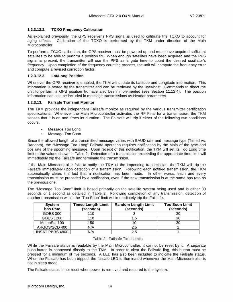
Microcom GTX-2.0 O&M Manual V2.20/R1
Microcom Design, Inc. 14
1.2.3.12.2. TCXO Frequency Calibration
As explained previously, the GPS receiver’s PPS signal is used to calibrate the TCXO to account for aging effects. Calibration of the TCXO is performed by the TKM under direction of the Main Microcontroller.
To perform a TCXO calibration, the GPS receiver must be powered up and must have acquired sufficient satellites to be able to perform a position fix. When enough satellites have been acquired and the PPS signal is present, the transmitter will use the PPS as a gate time to count the desired oscillator’s frequency. Upon completion of the frequency counting process, the unit will compute the frequency error and compute a revised correction factor.
1.2.3.12.3. Lat/Long Position
Whenever the GPS receiver is enabled, the TKM will update its Latitude and Longitude information. This information is stored by the transmitter and can be retrieved by the user/host. Commands to direct the unit to perform a GPS position fix have also been implemented (see Section 11.12.4). The position information can also be included in message transmissions as Header parameters.
1.2.3.13. Failsafe Transmit Monitor
The TKM provides the independent Failsafe monitor as required by the various transmitter certification specifications. Whenever the Main Microcontroller activates the RF Final for a transmission, the TKM senses that it is on and times its duration. The Failsafe will trip if either of the following two conditions occurs.
• Message Too Long • Message Too Soon
Since the allowed length of a transmitted message varies with BAUD rate and message type (Timed vs. Random), the “Message Too Long” Failsafe operation requires notification by the Main of the type and bps rate of the upcoming message. Upon receipt of this notification, the TKM will set its Too Long time limit to the values shown in Table 2. Detection of a transmission exceeding the appropriate time limit will immediately trip the Failsafe and terminate the transmission.
If the Main Microcontroller fails to notify the TKM of the impending transmission, the TKM will trip the Failsafe immediately upon detection of a transmission. Following each notified transmission, the TKM automatically clears the fact that a notification has been made. In other words, each and every transmission must be preceded by a notification, even if the new transmission is at the same bps rate as the previous one.
The “Message Too Soon” limit is based primarily on the satellite system being used and is either 30 seconds or 1 second as detailed in Table 2. Following completion of any transmission, detection of another transmission within the “Too Soon” limit will immediately trip the Failsafe.
System bps Rate
Timed Length Limit (seconds)
Random Length Limit (seconds)
Too Soon Limit (seconds)
GOES 300 110 3 30 GOES 1200 110 1.5 30
MeteoSat 100 150 10 30 ARGOS/SCD 400 N/A 2.5 1 INSAT PBRS 4800 N/A 2.5 1
Table 2: Failsafe Time Limits
While the Failsafe status is readable by the Main Microcontroller, it cannot be reset by it. A separate push-button is connected directly to the TKM. In order to clear the Failsafe flag, this button must be pressed for a minimum of five seconds. A LED has also been included to indicate the Failsafe status. When the Failsafe has been tripped, the failsafe LED is illuminated whenever the Main Microcontroller is not in sleep mode.
The Failsafe status is not reset when power is removed and restored to the system.
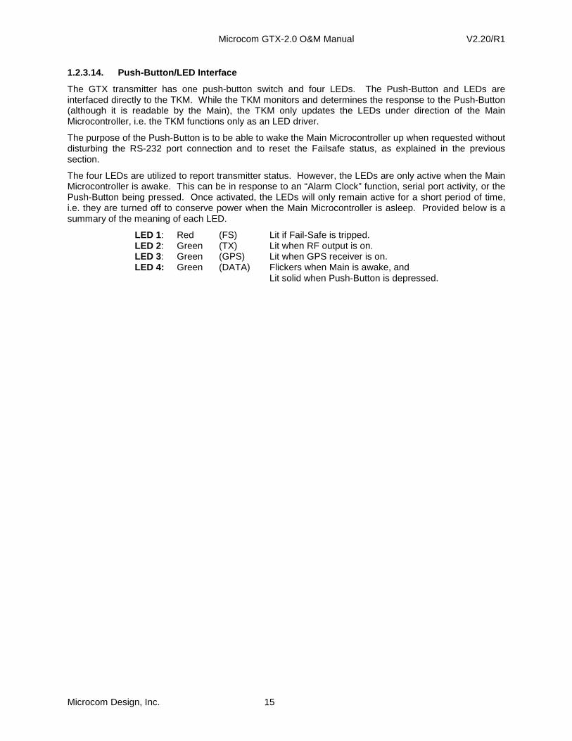
Microcom GTX-2.0 O&M Manual V2.20/R1
Microcom Design, Inc. 15
1.2.3.14. Push-Button/LED Interface
The GTX transmitter has one push-button switch and four LEDs. The Push-Button and LEDs are interfaced directly to the TKM. While the TKM monitors and determines the response to the Push-Button (although it is readable by the Main), the TKM only updates the LEDs under direction of the Main Microcontroller, i.e. the TKM functions only as an LED driver.
The purpose of the Push-Button is to be able to wake the Main Microcontroller up when requested without disturbing the RS-232 port connection and to reset the Failsafe status, as explained in the previous section.
The four LEDs are utilized to report transmitter status. However, the LEDs are only active when the Main Microcontroller is awake. This can be in response to an “Alarm Clock” function, serial port activity, or the Push-Button being pressed. Once activated, the LEDs will only remain active for a short period of time, i.e. they are turned off to conserve power when the Main Microcontroller is asleep. Provided below is a summary of the meaning of each LED.
LED 1: Red (FS) Lit if Fail-Safe is tripped. LED 2: Green (TX) Lit when RF output is on. LED 3: Green (GPS) Lit when GPS receiver is on. LED 4: Green (DATA) Flickers when Main is awake, and Lit solid when Push-Button is depressed.

Microcom GTX-2.0 O&M Manual V2.20/R1
Microcom Design, Inc. 16
2. GTX Hardware Set Up
The Microcom GTX is housed in a rugged, compact 6”x8”x1.5” aluminum enclosure. All connections to the transmitter are via end panel connectors as shown in Figure 1.
3
10
12.5Vdc
INPUT
+
1
-
OUT
RF
RF OUT
12.5Vdc
POWER
Satellite Data TransmitterGTX - 2.0
GPS
TX
FS TRIPPED
DATA
FS RESET
SDI-12
SERIAL
PORT
GPS ANT
5
6
11
8 9
7
4
2
FAILSAFE
RESET
DATA
I/O
TB
AB
DC
TG
RS-232
ANT
GPS
SDI-12
D+
-
GPS
TX
FS
I/0 / TB
Figure 1: GTX-2.0 Case
Referring to Figure 1, provided below is a list of the major end panel components.
1. Main Power Input Connector - +12.5 VDC 2. RF Output Connector 3. Tipping Bucket and Custom I/O Connector 4. GPS Antenna Connector 5. RS-232 Serial Port Connector 6. SDI-12 Interface Connector 7. Failsafe Reset Push-Button 8. LED4: Data Information LED (Green) 9. LED3: GPS Receive Active LED (Green)
10. LED2: RF Transmit Active LED (Green) 11. LED1: Failsafe Tripped LED (Red)
2.1. Connector Information
2.1.1. Main Power Connections
The main power input to the GTX is designed for a standard 12 Volt Lead Acid battery. The GTX-2.0 uses a keyed, locking, high current power connection, Molex P/N 50-84-2020; the mating connector is Molex P/N 50-84-1020.
The GTX-2.0 is supplied with a power cable to simplify the battery/power connection requirements. The supplied power cable consists of the mating connector with red and black wire leads; the red lead must be connected to the positive supply terminal and the black must be connected to the negative supply terminal. The supply lead ends are not terminated; user must provide the appropriate supply connections. Custom cables can also be provided by Microcom.
2.1.2. RF Output Connections
The RF Output connector (RF OUT) is a standard female SMA RF connector. External cabling must be provided to connect the RF Output to the GOES transmit antenna. For minimal cost, Microcom can provide the GOES transmit antenna cable. The standard cable is SMA-to-N with 20’ of LMR-240. Custom lengths and antenna connections can also be provided.

Microcom GTX-2.0 O&M Manual V2.20/R1
Microcom Design, Inc. 17
2.1.3. Tipping Bucket and Custom I/O Connections
The Tipping Bucket and I/O interface is a multipurpose connection point provided via a four position terminal block with detachable header as shown in Figure 2; Figure 1 shows the I/O and TB interface connector with the header removed. The interface connector is a Phoenix Contact P/N 1881464, and the detachable header is P/N 1881341.
The detachable header provides a zero insertion force compression connection that can accept wire sizes from 20 to 26 AWG. To insert the individual wires, a small tool is required to depress the compression release tab located above the wire receptacle. Once depressed, the wire can be inserted and the tab can be released locking the wire in place.
When viewed from the end panel, the “I/O TB” connector pins are designated A B C D T G left to right as shown in Figure 2.
Tipping Bucket
I/O
C
TB
GTDGPSANT BA
Figure 2: Tipping Bucket Interface Connections
The primary purpose of this connector is to provide a normally-open contact closure Tipping Bucket interface to the GTX’s internal counter. The connections for the Tipping Bucket must be made to pins T and G (ground) as shown in Figure 2.
The remaining four contacts (A through D) are routed to an internal connector that provides an interface to one of a variety of GTX option boards. These optional connections can be used to provide backup battery or analog inputs, an additional serial port, switched supply outputs, or other custom application specific signals as required. The specific connectivity is option board dependant.
As an example, if the GTX is ordered with the BBU-RTC option (see Section 1.2.3.10) this connector provides the input point for an external 3.6V Lithium battery to power the BBU-RTC when the GTX loses main power or the main battery voltage falls below the cutoff level. The connection points for the backup battery are shown in Figure 3; the positive lead of the battery connects to A and the negative lead connects to B.
Backup Battery
I/O
C
TB
GTDGPSANT BA
Figure 3: Battery Backup Interface Connections
2.1.4. GPS Antenna Connections
The GPS Antenna connector (GPS ANT) is a standard female MCX RF connector. The GPS Antenna connection must be interfaced to either a Trimble 3V Bullet (P/N 48360) or a Trimble 3V Magnetic-Mount Patch (39265-50) antenna. The GTX-2.0 comes standard with the 3V Bullet Antenna, but does not include an interface cable. If desired Microcom can alternately supply the magnetic-mount antenna or

Microcom GTX-2.0 O&M Manual V2.20/R1
Microcom Design, Inc. 18
can supply the interface cable for the Bullet antenna (the Magnetic Mount antenna incorporates a 5M cable). The standard Bullet interface cable is MCX-to-TNC with 20’ of LMR-240; custom lengths can also be provided.
2.1.5. RS-232 Serial Port Connections
The RS-232 Serial Port connector provides the host interface. The connector is a standard 9-pin female Sub-D connector.
Table 3 provides the signal connection for the 9-pin female Sub-D connector. Note that the signal names are referenced to the GTX-2.0; e.g. the TXD line is the transmit output from the GTX, which should be connected to the receive input of the host. All signals are true bipolar RS-232 levels.
Pin Number Signal 1 N/C 2 TXD 3 RXD 4 N/C 5 GND 6 N/C 7 RTS 8 CTS 9 N/C
Table 3: RS-232 Serial Port Pin-out
The connections shown in Table 3 allow the transmitter to be directly connected to a standard COMM port on a PC using a straight-through 9 conductor RS-232 patch cable.
Use of the RTS and CTS lines are optional as explained in Sections 1.2.3.11.2 and 3.1.
2.1.6. SDI-12 Connections
The SDI-12 connector provides an industry standard SDI-12 serial interface. The 3-pin connector provides a 1A recoverable PTC (Positive Temperature Coefficient thermistor) fused supply output, a serial data line, and ground (battery negative). The screw terminal connector is a Phoenix Contact P/N 1757255 with the detachable header P/N 1757022.
The detachable header provides a zero insertion force compression connection that can accept wire sizes from 12 to 24 AWG. To insert the wires, a small flat blade screwdriver is required to open and close the wire compression contact.
When viewed from the end panel, the SDI-12 connector pins are numbered 1 through 3 from left to right as shown in Figure 4; pin 1 is +V, pin 2 is Data, and pin 3 is GND.
RESETFAILSAFE
DATA RS-232
321
+V GND
Data
Figure 4: SDI-12 Interface Connector
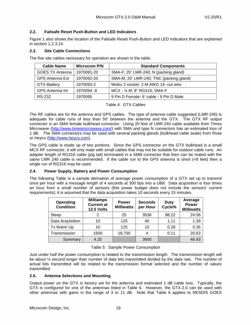
Microcom GTX-2.0 O&M Manual V2.20/R1
Microcom Design, Inc. 19
2.2. Failsafe Reset Push-Button and LED Indicators
Figure 1 also shows the location of the Failsafe Reset Push-Button and LED indicators that are explained in section 1.2.3.14.
2.3. Site Cable Connections
The five site cables necessary for operation are shown in the table.
Cable Name Microcom P/N Standard Components
GOES TX Antenna 1970091-20 SMA-F; 20’ LMR-240; N (packing gland)
GPS Antenna Ext 1970092-20 SMA-M; 20’ LMR-240; TNC (packing gland)
GTX-Battery 1970093-2 Molex 2 socket- 2 M AWG 14- cut wire
GPS Antenna Int 1970094-.8 MCX - ¼ M; 8” RG316; SMA-F
RS-232 1970095 9 Pin D Female- 6’ cable - 9 Pin D Male
Table 4: GTX Cables
The RF cables are for the antenna and GPS cables. The type of antenna cable suggested (LMR-240) is adequate for cable runs of less than 50’ between the antenna and the GTX. The GTX RF output connector is an SMA female bulkhead connector. Using 20 feet of LMR-240 cable available from Times Microwave (http://www.timesmicrowave.com/) with SMA and type N connectors has an estimated loss of 1 dB. The SMA connectors may be used with several packing glands (bulkhead cable seals) from Rose or Heyco (http://www.heyco.com).
The GPS cable is made up of two portions. Since the GPS connector on the GTX bulkhead is a small MCX RF connector, it will only mate with small cables that may not be suitable for outdoor cable runs. An adapter length of RG316 cable (pig tail) terminated in a SMB connector that then can be mated with the same LMR 240 cable is recommended. If the cable run to the GPS antenna is short (<8 feet) then a single run of RG316 may be used.
2.4. Power Supply, Battery and Power Consumption
The following Table is a sample derivation of average power consumption of a GTX set up to transmit once per hour with a message length of 4 seconds at 300 bps into a UB8. Data acquisition is four times an hour from a small number of sensors (this power budget does not include the sensors’ current requirements); it is assumed that the data acquisition takes 10 seconds every 15 minutes.
Operating Condition
Milliamps Current at 12.5 Volts
Power Milliwatts
Seconds per Hour
Duty Cycle%
Average Power
Milliwatts Sleep 2 25 3536 98.22 24.56
Data Acquisition 10 125 40 1.11 1.39
Tx Warm Up 10 125 10 0.28 0.35
Transmission 1500 18,750 4 0.11 20.63
Summary 4.25 3600 46.93
Table 5: Sample Power Consumption
Just under half the power consumption is related to the transmission length. The transmission length will be about ½ second longer than number of data bits transmitted divided by the data rate. The number of actual bits transmitted will be related to the transmission format selected and the number of values transmitted.
2.5. Antenna Selections and Mounting
Output power on the GTX is factory set for the antenna and estimated 1 dB cable loss. Typically, the GTX is configured for one of the antennas listed in Table 6. However, the GTX-2.0 can be used with other antennas with gains in the range of 3 to 11 dB. Note that Table 6 applies to NESDIS GOES

Microcom GTX-2.0 O&M Manual V2.20/R1
Microcom Design, Inc. 20
operation only; contact Microcom for information on antenna selection and maximum powers for use on other satellite systems.
Antenna Manufacturer
Model
Gain dB
Max Power 300 (Watts)
Max Power 1200 (Watts)
Microcom Design UB6 (XPress) 6 2.5 N/A Microcom Design UB8 8 1.6 5.0 Synergetics 18B-N 11 0.8 3.0
Table 6: Antenna Selection for GOES Operation
In order to ensure optimum operation, it is necessary to properly aim the transmit antenna. Appendix C: provides the necessary azimuth and elevation curves for any Latitude and Longitude within the satellite’s look angle.

Microcom GTX-2.0 O&M Manual V2.20/R1
Microcom Design, Inc. 21
3. GTX-2.0 Basic Operation and Configuration
Prior to placing the GTX-2.0 into service, the unit must be properly configured for the intended application. Configuring the GTX for operation consists of setting up the data collection functions and/or the transmission parameters.
The GTX may be configured using the intuitive command line interface using either a PC, a PalmTop, or a PDA. Microcom also provides an easy-to-use Windows© based configuration utility.
In either case, the host computer must have a standard RS-232 port to perform the configuration. The following sections provide an overview of both configuration methods; additional information with regard to configuring a specific function is provided throughout the remainder of this manual. Section 0 provides a complete reference for the serial port command interface.
3.1. Terminal Interface
The GTX was designed with a highly versatile and intuitive RS-232 port ASCII command line interface, which allows complete configuration via a terminal program, such as Windows© HyperTerminal. The interface is also suitable for connection to data loggers equipped with an RS-232 port. By utilizing an ASCII command line interface (as opposed to a menu system), common configurations can be captured in a text editor, which can be edited and easily downloaded to other units to facilitate configuring multiple units with similar setups.
The RS-232 port communicates at 9600 BAUD with 8 data bits, no parity and 1 stop bit. The serial port interface implements the RS-232 standard TXD, RXD, RTS, and CTS signals. While the handshake lines (RTS & CTS) are provided, the GTX is also designed to work with just the data lines (TXD & RXD). In other words, only the TXD, RXD, and ground connections are absolutely required for proper communications.
With few exceptions, all commands are a three character alphanumeric abbreviation or acronym of the command functionality. Certain commands that are more than three alphanumeric characters in length to prevent them from being inadvertently entered. Throughout this manual, the three-character commands are shown in all uppercase and are bolded. Any commands that are longer than three characters are shown in mixed case for readability. In actual use, the GTX command set is case insensitive, i.e. the GTX will accept any combination of upper and lower case characters.
Many commands are used to set or retrieve various configuration/calibration parameters. When setting parameters, the command is followed by an equals sign (‘=’). When retrieving parameters, the command is followed by a question mark (‘?’).
Certain commands are used to direct the transmitter to execute a specific function (e.g. clear a buffer); in such cases, neither a ‘=’ or a ‘?’ is utilized. Some of these commands may allow an optional parameter that further defines what action(s) will be executed. In this case, an equals sign may be utilized.
3.1.1. Typical Command Usage
Figure 5 shows a typical command line sequence to set up a GTX for an hourly timed transmission using a terminal interface. Following configuring the GTX for GOES mode (GTX=1), the command sequence sets the NOAA/NESDIS supplied parameters; i.e. the DCP’s Platform ID, the GOES channel and data rate, the self-timed transmission interval of 1 hour, the start time of the window assignment, and the window length. Following this information, the example in Figure 5 configures some of the user determinable settings; i.e. the message data format (ASCII), the message data source (RS-232), and the Timed Operational Flags.
Figure 6 shows a typical response to the Read Configuration (RCF?) command. The first ten lines of the response parrot the commands that were used to configure Timed operation in the example of Figure 5. The remaining lines show the current configuration for Random transmission operation. Using the Read Configuration command, the user can capture the setup to a text file that can then be edited and downloaded to another GTX.
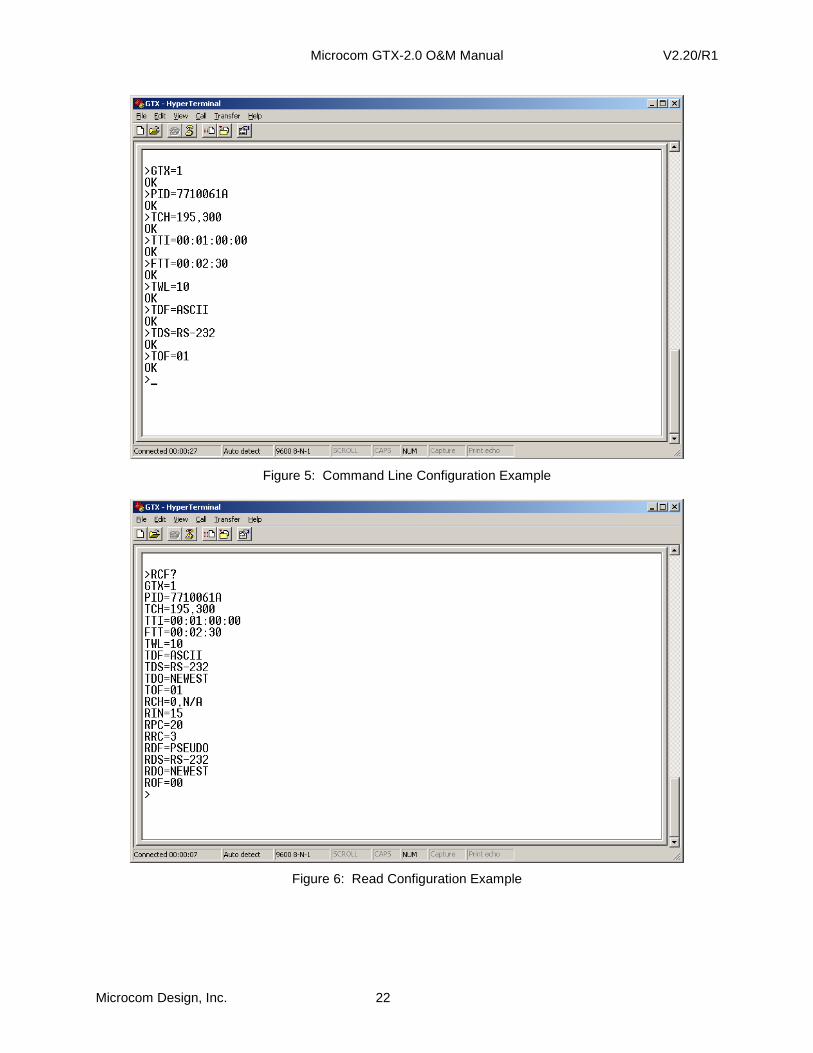
Microcom GTX-2.0 O&M Manual V2.20/R1
Microcom Design, Inc. 22
Figure 5: Command Line Configuration Example
Figure 6: Read Configuration Example
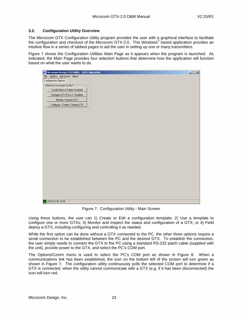
Microcom GTX-2.0 O&M Manual V2.20/R1
Microcom Design, Inc. 23
3.2. Configuration Utility Overview
The Microcom GTX Configuration Utility program provides the user with a graphical interface to facilitate the configuration and checkout of the Microcom GTX-2.0. This Windows© based application provides an intuitive flow in a series of tabbed pages to aid the user in setting up one or many transmitters.
Figure 7 shows the Configuration Utilities Main Page as it appears when the program is launched. As indicated, the Main Page provides four selection buttons that determine how the application will function based on what the user wants to do.
Figure 7: Configuration Utility - Main Screen
Using these buttons, the user can 1) Create or Edit a configuration template; 2) Use a template to configure one or more GTXs; 3) Monitor and Inspect the status and configuration of a GTX; or 4) Field deploy a GTX, including configuring and controlling it as needed.
While the first option can be done without a GTX connected to the PC, the other three options require a serial connection to be established between the PC and the desired GTX. To establish the connection, the user simply needs to connect the GTX to the PC using a standard RS-232 patch cable (supplied with the unit), provide power to the GTX, and select the PC’s COM port.
The Options/Comm menu is used to select the PC’s COM port as shown in Figure 8. When a communications link has been established, the icon on the bottom left of the screen will turn green as shown in Figure 7. The configuration utility continuously polls the selected COM port to determine if a GTX is connected; when the utility cannot communicate with a GTX (e.g. if it has been disconnected) the icon will turn red.

Microcom GTX-2.0 O&M Manual V2.20/R1
Microcom Design, Inc. 24
Figure 8: Configuration Utility - Options/Comm Menu
3.2.1. Create/Open A Setup Template
Selecting “Create/Open A Setup Template” allows the user to create new configuration template or edit an existing template. Template configurations provide a mechanism to define common setups that can be used for multiple GTX transmitters/data loggers. The template can then be used as baseline for configuring several units using the “Configure GTX From A Template” mode (see Section 3.2.2).
Figure 9: Configuration Utility - Create/Open A Setup Template
Once the “Create/Open A Setup Template” option is selected, additional page tab buttons become visible to allow the template to be defined as shown in Figure 9. For example, selecting the General Setup tab, allows the user to configure the GTX’s basic characteristics as shown in Figure 10. The first step in configuring the GTX is to Determine the type and number of “Configuration Quantities” that will be

Microcom GTX-2.0 O&M Manual V2.20/R1
Microcom Design, Inc. 25
required. As explained, in Section 5, the GTX-2.0 uses a soft approach to its configuration memory. This allows the available memory to be tailored to the specific needs of each user and/or platform.
Figure 10: Configuration Utility – Configuration Quantities
Once the “Configuration Quantities” are selected and saved, additional tabbed pages may become visible. In the example of Figure 10, the changes made added the “Transmission Setup”, “SDI-12 Sensors”, “Internal Sensors”, “Sensor Min Max Avg”, “Timed Data Buffer”, and “Random Triggers” tabs.
Once these additional tabs are available, the user can continue with the definition of the Template. After the configuration template has been fully defined, it can be saved using the File/Save Template menu item as shown in Figure 11.
Figure 11: Configuration Utility - File Menu
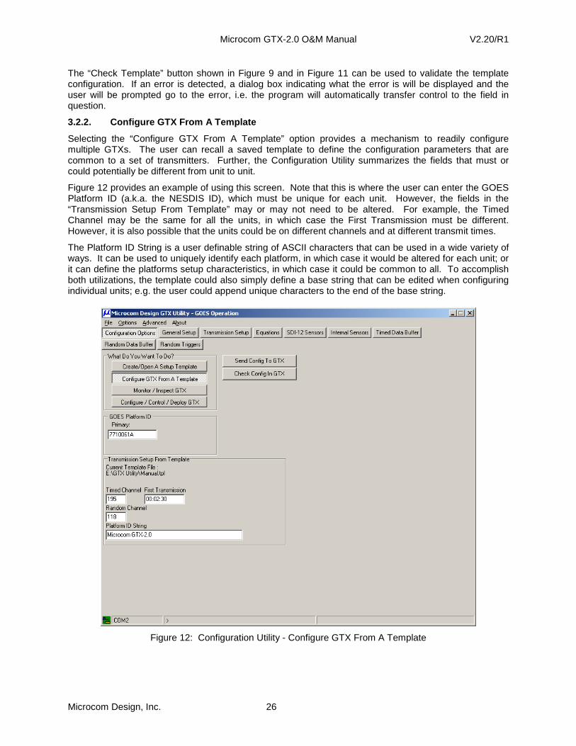
Microcom GTX-2.0 O&M Manual V2.20/R1
Microcom Design, Inc. 26
The “Check Template” button shown in Figure 9 and in Figure 11 can be used to validate the template configuration. If an error is detected, a dialog box indicating what the error is will be displayed and the user will be prompted go to the error, i.e. the program will automatically transfer control to the field in question.
3.2.2. Configure GTX From A Template
Selecting the “Configure GTX From A Template” option provides a mechanism to readily configure multiple GTXs. The user can recall a saved template to define the configuration parameters that are common to a set of transmitters. Further, the Configuration Utility summarizes the fields that must or could potentially be different from unit to unit.
Figure 12 provides an example of using this screen. Note that this is where the user can enter the GOES Platform ID (a.k.a. the NESDIS ID), which must be unique for each unit. However, the fields in the “Transmission Setup From Template” may or may not need to be altered. For example, the Timed Channel may be the same for all the units, in which case the First Transmission must be different. However, it is also possible that the units could be on different channels and at different transmit times.
The Platform ID String is a user definable string of ASCII characters that can be used in a wide variety of ways. It can be used to uniquely identify each platform, in which case it would be altered for each unit; or it can define the platforms setup characteristics, in which case it could be common to all. To accomplish both utilizations, the template could also simply define a base string that can be edited when configuring individual units; e.g. the user could append unique characters to the end of the base string.
Figure 12: Configuration Utility - Configure GTX From A Template

Microcom GTX-2.0 O&M Manual V2.20/R1
Microcom Design, Inc. 27
As shown in Figure 12, the “Configure GTX From A Template” page provides a button to send the configuration to the GTX. A second button allows the configuration to be validated in the GTX after download.
When configuring a GTX from a template, the user has the option to lock out any changes to configuration parameters except for those shown in Figure 12. The default case is to allow the user to view the template settings on the setup pages, but the editing controls are disabled. To enable template editing in this mode, use the Options/Preferences menu item to call up the “GTX Configuration Preferences” dialog; select the “Configuration” tab and check the “Allow Template Mod when Configuring GTX from Template” box.
3.2.3. Monitor/Inspect GTX
The “Monitor/Inspect GTX” option allows the user to quickly, and easily, get status information for a unit. While this option can be used any time a GTX is connected to the PC, it is most useful for checking the status of operational platforms, i.e. when the GTX is enabled.
In this mode, the Configuration Utility periodically polls the connected GTX for it’s current status. The status information is summarized in a set of tabbed pages as shown in Figure 13, with the unit’s Platform ID provided at the top of the tab sheets.
Figure 13: Configuration Utility - Monitor/Inspect GTX Information
Using the various tab sheets, the user can get a “GTX Information” summary (see Figure 13), data on the “Last Transmission” (see Figure 81), and current “GPS Status” (see Figure 88). Tabs are also provided to view the last sample value and when the next sample will be taken from either the Internal or SDI-12 Sensors as shown in the example of Figure 14. The user can even view the data in the Timed (see Figure 54) and Random (see Figure 57) transmission buffers.

Microcom GTX-2.0 O&M Manual V2.20/R1
Microcom Design, Inc. 28
The “Retrieve Config From GTX” button can be used to upload the entire configuration setup, which can then be viewed (but not edited) using the main setup tab buttons.
Figure 14: Configuration Utility - Monitor/Inspect SDI-12 Sensors
3.2.4. Configure/Control/Deploy GTX
The “Configure/Control/Deploy GTX” option provides total control of the GTX. In this mode, the user can completely configure the unit, if it has not already been done. This option also provides several controls to prepare the unit for operation, and to deploy it.
As shown in Figure 15, this page allows the user to Set or Read the GTX’s clock; Preset or Read the UTC correction; upload, download, and verify configurations; and Enable (in either transmitter or Data Logger mode) and Disable the GTX. This page also provides a button to reset all configuration settings to their factory default values.
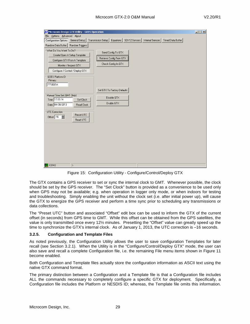
Microcom GTX-2.0 O&M Manual V2.20/R1
Microcom Design, Inc. 29
Figure 15: Configuration Utility - Configure/Control/Deploy GTX
The GTX contains a GPS receiver to set or sync the internal clock to GMT. Whenever possible, the clock should be set by the GPS receiver. The “Set Clock” button is provided as a convenience to be used only when GPS may not be available; e.g. when operation in logger only mode, or when indoors for testing and troubleshooting. Simply enabling the unit without the clock set (i.e. after initial power up), will cause the GTX to energize the GPS receiver and perform a time sync prior to scheduling any transmissions or data collections.
The “Preset UTC” button and associated “Offset” edit box can be used to inform the GTX of the current offset (in seconds) from GPS time to GMT. While this offset can be obtained from the GPS satellites, the value is only transmitted once every 12½ minutes. Presetting the “Offset” value can greatly speed up the time to synchronize the GTX’s internal clock. As of January 1, 2013, the UTC correction is –16 seconds.
3.2.5. Configuration and Template Files
As noted previously, the Configuration Utility allows the user to save configuration Templates for later recall (see Section 3.2.1). When the Utility is in the “Configure/Control/Deploy GTX” mode, the user can also save and recall a complete Configuration file, i.e. the remaining File menu items shown in Figure 11 become enabled.
Both Configuration and Template files actually store the configuration information as ASCII text using the native GTX command format.
The primary distinction between a Configuration and a Template file is that a Configuration file includes ALL the commands necessary to completely configure a specific GTX for deployment. Specifically, a Configuration file includes the Platform or NESDIS ID; whereas, the Template file omits this information.

Microcom GTX-2.0 O&M Manual V2.20/R1
Microcom Design, Inc. 30
Further, a Configuration file also has a CFS (Configuration Save, see Section 11.9.2) command at the end of the file.
3.3. Terminal versus Configuration Utility
As detailed in Section 3.2.5, the Configuration Utility utilizes the GTX command set to save configuration files. Further, the Configuration Utility simply encapsulates the GTX’s terminal protocol and command set into a graphical interface. In other words, any operation that can be accomplished from the Configuration Utility can also be done using a Terminal interface. Section 11 provides a complete description of the GTX’s command set.
Since the Configuration Utility saves the configuration information as GTX commands in text files, these files can also be used by Terminal applications to download the configuration when the Configuration Utility is not available, i.e. from a PDA or a PalmTop.
Further, since the Configuration Utility is designed to communicate with the GTX using it’s standard command set, it is also possible to issue direct commands to the GTX from the Utility. By accessing the Advanced/GTX Control menu item as shown in Figure 16, the user can launch the GTX Direct Control dialog shown in Figure 17.
Figure 16: Configuration Utility - Advanced Menu
Using this dialog, the user can issue any command to the GTX and view the response in the memo field. This dialog can be useful to quickly check out a GTX or even change a configuration parameter without affecting the configuration or template currently being worked on.
For example, Figure 17 shows how this dialog can be used to query the status of the connected GTX to ensure its configuration can be altered, i.e. the unit is Disabled. Once verified, the FTT? Command is used to query for the current value for the time of first transmission (i.e. the start of the self-timed window). Next, this parameter is changed to 00:47:00, and a CFS command is issued to commit the change to permanent memory.
Performing such a sequence through direct control, allows a GTX configuration parameter to be updated without affecting any of the settings on the various configuration pages.

Microcom GTX-2.0 O&M Manual V2.20/R1
Microcom Design, Inc. 31
Figure 17: Configuration Utility - GTX Direct Control
3.4. Enabled versus Disabled Operation
The GTX-2.0 operates in one of two main states, Enabled or Disabled. Either the Terminal Interface or the Configuration Utility can be used to transition the GTX back and forth between the Enabled and Disabled state. To deploy a GTX for operation, it must be placed in the Enabled state.
In the Disabled state, the GTX can be configured. It will not automatically collect data from sensors or send transmissions. However, test commands have been provided to perform these functions for test and troubleshooting. In the Disabled state, the GTX’s Main Microcontroller always remains awake (i.e. does not enter it’s low power sleep state) and the RS-232 port is continuously enabled.
In the Enabled state, the GTX’s configuration can NOT be altered. In this state, the unit will collect data from sensors based on the configured schedules, and will transmit normally, i.e. according to the self-timed schedule or send random transmission in response to triggering events. When the GTX is enabled, the unit will also automatically enter the sleep mode to reduce current consumption. In order to send RS-232 commands, the user or host data logger must first wake up the unit before it will respond to RS-232 commands.
Note that the Configuration Utility’s “Monitor/Inspect GTX” (see Section 3.2.3) mode will provide sufficient serial port activity to keep the unit out of sleep mode even when it’s Enabled.
While the user can NOT send test transmissions when a GTX is Enabled, commands can be issued to obtain feedback from the Internal and SDI-12 Sensors to confirm proper operation without disabling the unit.
3.4.1. Transmitter versus Data Logger Functions – S etting the GTX Operation Mode
The GTX-2.0 provides both satellite transmission and data logging capabilities. While the most common application will utilize both these capabilities, the GTX can be used as a transmitter only and as a data logger only.
When utilizing the GTX as a transmitter only, the bulk of the data to transmit is provided from an external device via the serial interface, i.e. the Timed or Random Data Source (TDS or RDS) is set to RS-232. However, configuring the GTX to operate in this manner does not preclude the use of the data logger functions, i.e. the GTX can still be configured to sample sensors and log their data, but the sampled data
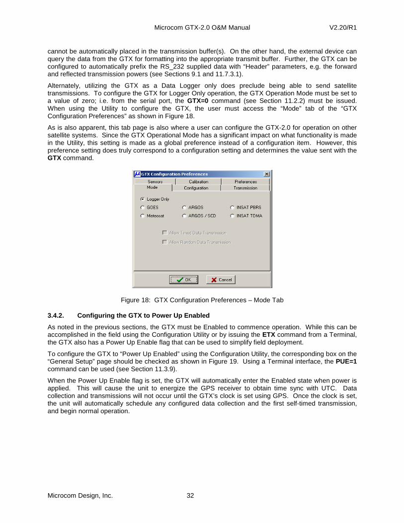
Microcom GTX-2.0 O&M Manual V2.20/R1
Microcom Design, Inc. 32
cannot be automatically placed in the transmission buffer(s). On the other hand, the external device can query the data from the GTX for formatting into the appropriate transmit buffer. Further, the GTX can be configured to automatically prefix the RS_232 supplied data with “Header” parameters, e.g. the forward and reflected transmission powers (see Sections 9.1 and 11.7.3.1).
Alternately, utilizing the GTX as a Data Logger only does preclude being able to send satellite transmissions. To configure the GTX for Logger Only operation, the GTX Operation Mode must be set to a value of zero; i.e. from the serial port, the GTX=0 command (see Section 11.2.2) must be issued. When using the Utility to configure the GTX, the user must access the “Mode” tab of the “GTX Configuration Preferences” as shown in Figure 18.
As is also apparent, this tab page is also where a user can configure the GTX-2.0 for operation on other satellite systems. Since the GTX Operational Mode has a significant impact on what functionality is made in the Utility, this setting is made as a global preference instead of a configuration item. However, this preference setting does truly correspond to a configuration setting and determines the value sent with the GTX command.
Figure 18: GTX Configuration Preferences – Mode Tab
3.4.2. Configuring the GTX to Power Up Enabled
As noted in the previous sections, the GTX must be Enabled to commence operation. While this can be accomplished in the field using the Configuration Utility or by issuing the ETX command from a Terminal, the GTX also has a Power Up Enable flag that can be used to simplify field deployment.
To configure the GTX to “Power Up Enabled” using the Configuration Utility, the corresponding box on the “General Setup” page should be checked as shown in Figure 19. Using a Terminal interface, the PUE=1 command can be used (see Section 11.3.9).
When the Power Up Enable flag is set, the GTX will automatically enter the Enabled state when power is applied. This will cause the unit to energize the GPS receiver to obtain time sync with UTC. Data collection and transmissions will not occur until the GTX’s clock is set using GPS. Once the clock is set, the unit will automatically schedule any configured data collection and the first self-timed transmission, and begin normal operation.

Microcom GTX-2.0 O&M Manual V2.20/R1
Microcom Design, Inc. 33
Figure 19: Configuration Utility - General Setup Page
3.5. GPS Time Sync and TCXO Calibration Settings
As indicated in Figure 19, the General Setup tab page is also where the user can configure the GPS Time Sync and TCXO Calibration options. Specifically, four controls are provided in the “GPS Time Sync” group to customize this functionality.
First, the user can specify how often, in hours, the GPS receiver is energized to synchronize the GTX’s internal clock. The default setting is 24 hours, or once a day.
Second, an option is provided to configure how often the GTX will calibrate the internal TCXO using the GPS receiver. The default is once every 10 days, which should be adequate for most applications. Note, to maintain the required transmit frequency accuracy for GOES operation, the GTX-2.0 MUST perform a TCXO calibration at least once every 20 days. Otherwise, per NOAA/NESDIS requirements, the GTX will discontinue making transmissions. However, all data collection functions will remain active.
The third parameter is a timeout value in minutes. If the GPS receiver can not acquire sufficient satellites to perform a Time Sync or TCXO Calibration in the specified time, e.g. 15 minutes, the operation will be aborted and re-scheduled for the next hour. This timeout is simply to minimize current drain on the system battery if some fault exists in the GPS subsystem.
Finally, checking the Log GPS Calibration box directs the GTX to log any occurrence of a GPS Time Sync, or TCXO Calibration in the event buffer. When a Time Sync event is logged, it’s time stamp is the actual time sync of the event and the data saved is the GTX’s clock error just prior to the synchronization; this value is measured an stored in seconds with millisecond resolution. When the GTX logs a TCXO calibration, the correction factor in parts per million is logged.

Microcom GTX-2.0 O&M Manual V2.20/R1
Microcom Design, Inc. 34
The TCXO Calibration and Sync Timeout settings are considered "Advanced Settings”. While these parameters are always visible, they are only enabled for edit when the “Advanced Settings” menu option in the “Advanced” menu is checked.
Each of the four settings discussed above has a corresponding serial command (GTS, GTC, GTO, and GLG) associated discussed in Section 11.8.

Microcom GTX-2.0 O&M Manual V2.20/R1
Microcom Design, Inc. 35
4. GTX Operation with GOES
This section provides an overview of the required setup of the GTX for operation on the GOES DCS system.
4.1. GOES DCS Description
A more complete description of the GOES DCS is included on the references in the appendices. The description here is given to aid in the initial operating set up of the GTX.
GOES DCS is a US supported system for the collection of environmental data. Its principal components are the geosynchronous spacecrafts (East and West), NOAA’s Command and Data Acquisition Station (CDA) located at Wallops Island, and the Remote Data Collection Platform (DCP) transmitters. These elements are shown in the Figure 20.
GOESSPACECRAFT
WEST
GOESSPACECRAFT
EAST
NOAA WALLOPS CDASTATION
4.8 METERANTENNA
7 METERANTENNA
PILOT SIGNAL TOGOES EAST AND
WEST SPACECRAFT
FIELD ofREMOTE
DCPs
Figure 20: Major Elements of GOES DCS
The spacecrafts are located at 75 W (GOES East) and 135 W (GOES West) longitude and zero latitude positions at a geosynchronous altitude of 22,500 miles above the earth’s surface. The remote DCPs transmit in a frequency band about 402 MHz. The downlink from the spacecraft is at 1694 MHz and includes the DCS signals from the remote sites along other weather data, e.g. earth imagery. These frequencies are reserved internationally for exclusive use in this service.
GOES DCS is part of a worldwide system of satellites that provide global coverage for environmental observations. Some of the other satellite based systems are shown in Table 7 below.
System Location(s) Operator Comments
METEOSAT 0 Eumetsat
INSAT 80 E and 87 E INSRO of India
GMS 140 E Japan Met
ARGOS Polar Orbit French Government Uses NOAA polar satellites.
Table 7: Related Satellite Data Collection Systems
Microcom GTX-2.0 O&M Manual V2.20/R1
Microcom Design, Inc. 36
In all of these cases the satellite functions as a radio repeater where signals in the specified frequency band are received by the satellite, amplified, converted in frequency and relayed to the ground receiving equipment of the system operator.
The system user provides the remote sensing equipment. Received data or messages may be obtained from the system Operator via various terrestrial communication links (e.g. the Internet). However, the system user may also provide their own satellite-receiving equipment, also known as a Direct Readout Ground Station (DRGS), to directly receive the remote transmissions.
Since the satellite repeater is shared by all users, its method of shared use is specified by the Operator. These methods of use and equipment must be agreed to by the system users.
The GTX-2.0 is certified for use on:
• GOES, all bands • METEOSAT International and Regional Bands • ARGOS/SCD • INSAT PBRS Mode • GMS
Currently the only operating method for GOES DCS is self-initiated; interrogation or polled operation is not currently supported. The GTX supports two methods of self-initiated operation, self-timed and random reporting. The self-timed mode uses the remote’s internal clock to trigger a data transmission. The random mode typically uses sensor activity to trigger a transmission sequence.
The frequency band of operation for GOES DCS uplink is 401.7 to 402.1 MHz. Per the second certification standard (CS2), the 400 kHz frequency band is divided into 532 channels of 750 Hz each for low rate operation of 300 bps. Portions of this same frequency band can be allocated to 1200 bps operation; in the latest standard, a 1200 bps channel requires three consecutive 750 Hz channel, or 2,250 Hz. In the original HDR certification standard (CS1), 300 bps channels were 1,500 kHz wide and 1200 bps channels were 3kHz wide. The allocation of 300 bps channels versus 1200 bps channels is solely at the discretion of NOAA/NESDIS, the GOES system Operator. For the foreseeable future, NOAA will be operating in both CS1 and CS2 mode, but CS1 and CS2 transmitters can share common channels.
NOAA/NESDIS (and other Operators) specifies the following items to the user:
• List of Certified Transmitters available for selection • Remote Platform ID of 8 Hex characters • Operating channel(s) • Operating data rate(s) • Self-Timed reporting slot • Random reporting daily transmission time loading
An example of received messages and their associated NOAA assigned time slots is shown in Figure 21. This screen shot is from Microcom’s DAMS-NT GOES DCS Tool Kit.
The yellow lines indicate the actual times of the received messages overlaying the assigned windows as indicated by the two-tone gray spaces. The messages would be ideally located in the center of the assigned time spaces.

Microcom GTX-2.0 O&M Manual V2.20/R1
Microcom Design, Inc. 37
Figure 21: Channel 49 GOES East Received Messages Overlaid Time Assigned Slots
4.2. Set Up for Use with Self-Timed Operation
The user should have on hand the following information:
� NOAA/NESDIS information for: • Reporting Channel and BAUD Rate, example is 195 at 300 bps • Reporting Time, e.g. 02:30 (in UTC/GMT not local time) • Reporting Interval, e.g. 60 minutes • Reporting Window length, e.g. 10 seconds
� GTX connected to Laptop, power supply, RF Load, GPS antenna.
Time given by NESDIS is the time after midnight of GMT on which the first transmission of that day will be made. The GTX’s clock must be set to GMT to ensure proper operation; this will be done automatically if the GTX’s internal clock is set using the integral GPS receiver.
The following subsections detail the procedures for setting up a GTX for Self-Timed operation. Both the Configuration Utility and the Terminal interface setup are covered. However, the information provided only covers the scheduling and formatting of self-timed transmissions; the procedures and set up information for loading data into the Timed transmission buffer will be covered in later sections.
4.2.1. Terminal Configuration for GOES Self-Timed O peration
Figure 5 provides an example of setting up the GTX for GOES Self-Timed operation. A total of six commands must be provided to properly schedule and format GOES self-timed transmissions; two additional commands (TDS & TDO) affect data storage in the Timed Buffer and are covered later.
Note that all the commands involving transmitter set up require the GTX to be placed in the Disabled mode (i.e. send the DTX command). Complete descriptions of all commands is provided in Section 11.2. Table 8 provides a summary of the commands required to complete the Self-Timed setup.
When using the Terminal Interface to setup a GTX, it is often helpful to perform an RCF (Read Configuration) command. This command prints out the current configuration and presents that information in the proper format as shown in Figure 6.
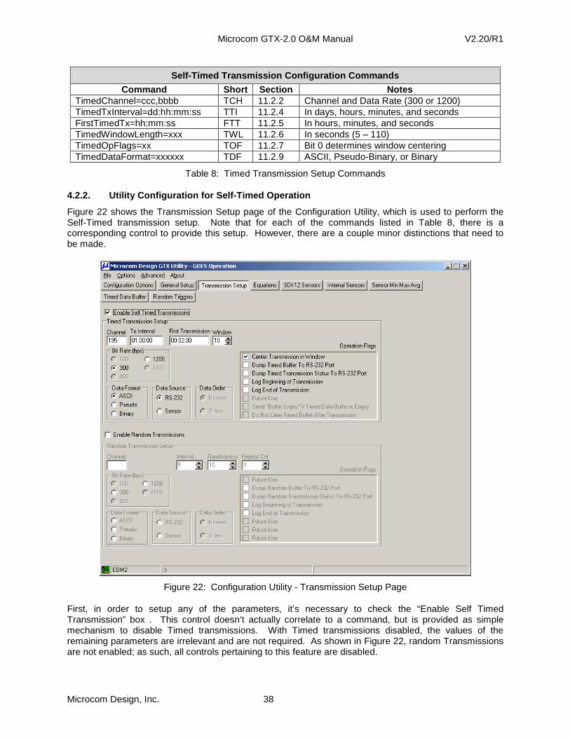
Microcom GTX-2.0 O&M Manual V2.20/R1
Microcom Design, Inc. 38
Self-Timed Transmission Configuration Commands
Command Short Section Notes TimedChannel=ccc,bbbb TCH 11.2.2 Channel and Data Rate (300 or 1200) TimedTxInterval=dd:hh:mm:ss TTI 11.2.4 In days, hours, minutes, and seconds FirstTimedTx=hh:mm:ss FTT 11.2.5 In hours, minutes, and seconds TimedWindowLength=xxx TWL 11.2.6 In seconds (5 – 110) TimedOpFlags=xx TOF 11.2.7 Bit 0 determines window centering TimedDataFormat=xxxxxx TDF 11.2.9 ASCII, Pseudo-Binary, or Binary
Table 8: Timed Transmission Setup Commands
4.2.2. Utility Configuration for Self-Timed Operati on
Figure 22 shows the Transmission Setup page of the Configuration Utility, which is used to perform the Self-Timed transmission setup. Note that for each of the commands listed in Table 8, there is a corresponding control to provide this setup. However, there are a couple minor distinctions that need to be made.
Figure 22: Configuration Utility - Transmission Setup Page
First, in order to setup any of the parameters, it’s necessary to check the “Enable Self Timed Transmission” box . This control doesn’t actually correlate to a command, but is provided as simple mechanism to disable Timed transmissions. With Timed transmissions disabled, the values of the remaining parameters are irrelevant and are not required. As shown in Figure 22, random Transmissions are not enabled; as such, all controls pertaining to this feature are disabled.

Microcom GTX-2.0 O&M Manual V2.20/R1
Microcom Design, Inc. 39
Second, the Tx Interval in the Configuration Utility only shows hours, minutes, and seconds. Since transmission intervals greater than 3 or 4 hours are atypical, the utility omits the days in the control and will force them to 00 when issuing the command. If daily intervals are required, this control can be set to include days by checking the “Allow Interval Days” box on the Transmission Setup page of the GTX Configuration Preferences dialog.
4.3. Set Up for Use with Random Operation
The user should have on hand the following information:
� NOAA/NESDIS information for: • Reporting Channel and BAUD Rate, example is 118 at 100 bps • Reporting Interval, e.g. 15 minutes • Reporting Repeat Count, e.g. 3 transmissions
� GTX connected to Laptop, power supply, RF Load, GPS antenna.
The following subsections detail the procedures for setting up a GTX for Random operation. Both the Configuration Utility and the Terminal interface setup are covered. However, the information provided only covers the scheduling and formatting of self-timed transmissions; the procedures and set up information for loading data into the Random transmission buffer will be covered in later sections.
4.3.1. Terminal Configuration for Random Operation
Figure 23 provides an example of setting up the GTX for Random operation using a Terminal interface. A total of six commands must be provided to properly schedule and format random transmissions; two additional commands (RDS & RDO) affect data storage in the Random Buffer and are covered later.
Note that all the commands involving transmitter set up require the GTX to be placed in the Disabled mode (i.e. send the DTX command). Complete descriptions of all commands is provided in Section 11.2. Table 9 provides a summary of the commands required to complete the Random setup.
Random Transmission Configuration Commands
Command Short Section Notes RandomChannel=ccc,bbbb RCH 11.2.12 Channel and BAUD rate (300 or 1200) RandomInterval=mm RIN 11.2.13 In minutes RandomPercent=pp RPC 11.2.14 In percent RandomRepeatCnt=xx RRC 11.2.15 RandomDataFormat =xxxxxxx RDF 11.2.16 ASCII, Pseudo-Binary, or Binary RandomOpFlags=xx ROF 11.2.19
Table 9: Random Transmission Setup Commands

Microcom GTX-2.0 O&M Manual V2.20/R1
Microcom Design, Inc. 40
Figure 23: Random Transmission Terminal Setup
When using the Terminal Interface to setup a GTX, it is often helpful to perform an RCF (Read Configuration) command. This command prints out the current configuration and presents that information in the proper format as shown in Figure 6.
4.3.2. Utility Configuration for Random Operation
Figure 24 shows the Transmission Setup page of the Configuration Utility, which is used to perform the Random transmission setup. Note that for each of the commands listed in Table 9, there is a corresponding control to provide this setup. However, there are a couple of minor distinctions that need to be made.
First, in order to setup any of the parameters, it’s necessary to check the “Enable Random Transmission” box. This control doesn’t actually correlate to a command, but is provided as simple mechanism to disable Random transmissions. With Random transmissions disabled, the values of the remaining parameters are irrelevant and are not required. Figure 23 shows this same page with Random transmissions not enabled; as such, controls pertaining to this feature are disabled.
Second, note also that there is not a Preamble control in the Random Transmission Setup group (see Figure 24) nor is there a command in Table 9 for this setting. The preamble type does not apply to HDR operation and Long Preambles are not permitted for Random transmission at 100 bps so this control is omitted.
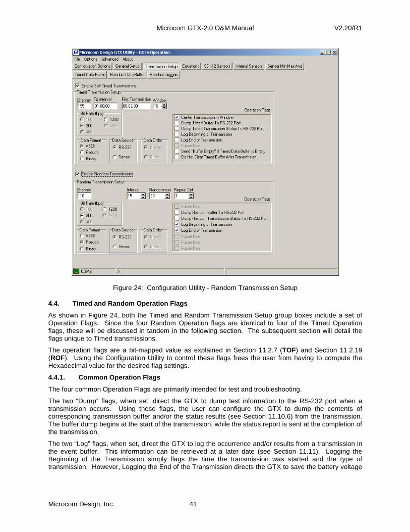
Microcom GTX-2.0 O&M Manual V2.20/R1
Microcom Design, Inc. 41
Figure 24: Configuration Utility - Random Transmission Setup
4.4. Timed and Random Operation Flags
As shown in Figure 24, both the Timed and Random Transmission Setup group boxes include a set of Operation Flags. Since the four Random Operation flags are identical to four of the Timed Operation flags, these will be discussed in tandem in the following section. The subsequent section will detail the flags unique to Timed transmissions.
The operation flags are a bit-mapped value as explained in Section 11.2.7 (TOF) and Section 11.2.19 (ROF). Using the Configuration Utility to control these flags frees the user from having to compute the Hexadecimal value for the desired flag settings.
4.4.1. Common Operation Flags
The four common Operation Flags are primarily intended for test and troubleshooting.
The two “Dump” flags, when set, direct the GTX to dump test information to the RS-232 port when a transmission occurs. Using these flags, the user can configure the GTX to dump the contents of corresponding transmission buffer and/or the status results (see Section 11.10.6) from the transmission. The buffer dump begins at the start of the transmission, while the status report is sent at the completion of the transmission.
The two “Log” flags, when set, direct the GTX to log the occurrence and/or results from a transmission in the event buffer. This information can be retrieved at a later date (see Section 11.11). Logging the Beginning of the Transmission simply flags the time the transmission was started and the type of transmission. However, Logging the End of the Transmission directs the GTX to save the battery voltage

Microcom GTX-2.0 O&M Manual V2.20/R1
Microcom Design, Inc. 42
under load, the forward power, and the reflected power in the event log. Recalling this data can provide useful information with regard to the performance of the unit over time.
4.4.2. Timed Only Operation Flags
Four additional flags applicable to Timed transmissions only are included in the Timed Operation Flags as shown in Figure 24.
4.4.2.1. Center Transmission in Window
The “Center Transmission in Window” flag, when set, directs the GTX to center the Timed transmission within the programmed transmission window. Specifically, prior to sending a Timed message, the GTX will compute the message length, subtracts this value from the TimedWindowLength , and adjust the transmission start time by one half of the difference. This process ensures that the message is precisely centered in the window.
Not setting this flag will direct the GTX to start the message at the top of window.
Centering the transmission in the window ensures the maximum protection from being interfered with by a platform in a neighboring window, especially when the message length is small compared to the window size. This approach can be critical to reliable message reception when neighboring windows are “owned” by another GOES user.
4.4.2.2. Timed Buffer Control Flags
The remaining two Timed Operation Flags are related to the Timed message buffer. Both of these flags are only applicable when the GTX is configured with RS-232 as the Data Source, i.e. when transmission data is provided by an external host.
The Send “Buffer Empty” flag directs the GTX to send the message “BUFFER EMPTY” if the Timed message buffer is empty at the start of a timed transmission.
The “Do Not Clear Timed Buffer” overrides the default operation of automatically clearing the Timed message buffer at completion of a transmission.
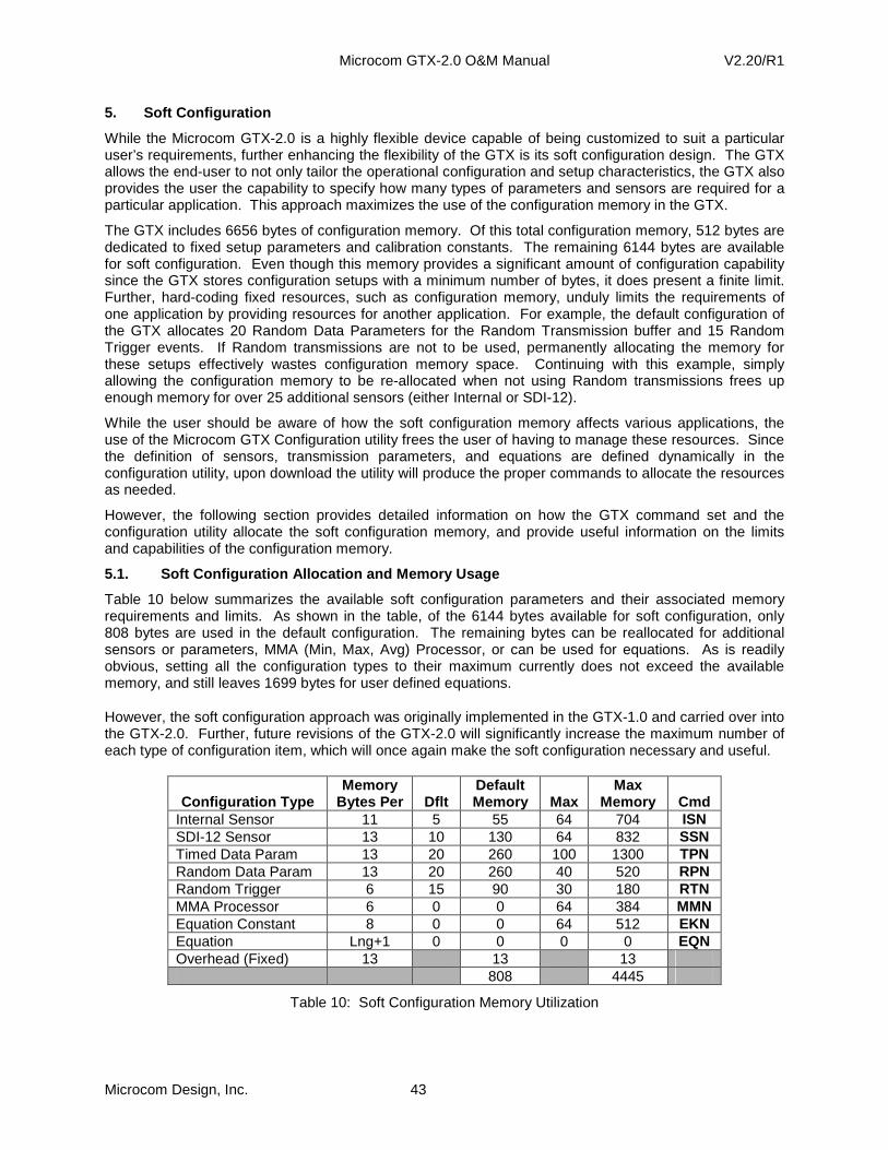
Microcom GTX-2.0 O&M Manual V2.20/R1
Microcom Design, Inc. 43
5. Soft Configuration
While the Microcom GTX-2.0 is a highly flexible device capable of being customized to suit a particular user’s requirements, further enhancing the flexibility of the GTX is its soft configuration design. The GTX allows the end-user to not only tailor the operational configuration and setup characteristics, the GTX also provides the user the capability to specify how many types of parameters and sensors are required for a particular application. This approach maximizes the use of the configuration memory in the GTX.
The GTX includes 6656 bytes of configuration memory. Of this total configuration memory, 512 bytes are dedicated to fixed setup parameters and calibration constants. The remaining 6144 bytes are available for soft configuration. Even though this memory provides a significant amount of configuration capability since the GTX stores configuration setups with a minimum number of bytes, it does present a finite limit. Further, hard-coding fixed resources, such as configuration memory, unduly limits the requirements of one application by providing resources for another application. For example, the default configuration of the GTX allocates 20 Random Data Parameters for the Random Transmission buffer and 15 Random Trigger events. If Random transmissions are not to be used, permanently allocating the memory for these setups effectively wastes configuration memory space. Continuing with this example, simply allowing the configuration memory to be re-allocated when not using Random transmissions frees up enough memory for over 25 additional sensors (either Internal or SDI-12).
While the user should be aware of how the soft configuration memory affects various applications, the use of the Microcom GTX Configuration utility frees the user of having to manage these resources. Since the definition of sensors, transmission parameters, and equations are defined dynamically in the configuration utility, upon download the utility will produce the proper commands to allocate the resources as needed.
However, the following section provides detailed information on how the GTX command set and the configuration utility allocate the soft configuration memory, and provide useful information on the limits and capabilities of the configuration memory.
5.1. Soft Configuration Allocation and Memory Usag e
Table 10 below summarizes the available soft configuration parameters and their associated memory requirements and limits. As shown in the table, of the 6144 bytes available for soft configuration, only 808 bytes are used in the default configuration. The remaining bytes can be reallocated for additional sensors or parameters, MMA (Min, Max, Avg) Processor, or can be used for equations. As is readily obvious, setting all the configuration types to their maximum currently does not exceed the available memory, and still leaves 1699 bytes for user defined equations.
However, the soft configuration approach was originally implemented in the GTX-1.0 and carried over into the GTX-2.0. Further, future revisions of the GTX-2.0 will significantly increase the maximum number of each type of configuration item, which will once again make the soft configuration necessary and useful.
Configuration Type
Memory Bytes Per
Dflt
Default Memory
Max
Max Memory
Cmd
Internal Sensor 11 5 55 64 704 ISN SDI-12 Sensor 13 10 130 64 832 SSN Timed Data Param 13 20 260 100 1300 TPN Random Data Param 13 20 260 40 520 RPN Random Trigger 6 15 90 30 180 RTN MMA Processor 6 0 0 64 384 MMN Equation Constant 8 0 0 64 512 EKN Equation Lng+1 0 0 0 0 EQN Overhead (Fixed) 13 13 13 808 4445
Table 10: Soft Configuration Memory Utilization

Microcom GTX-2.0 O&M Manual V2.20/R1
Microcom Design, Inc. 44
The far right column of Table 10 provides the GTX command that can be utilized to adjust the allocated memory for each configuration type. These commands are covered in detail in Section 11.
One other useful command when setting up the soft configuration for the GTX is the Configuration Memory Available (or CMA) command. This command allows the user to query the GTX for the number of soft configuration bytes currently available. In other words, this command frees the user of having to calculate the available memory in the soft configuration memory based on the current definitions.
Microcom GTX-2.0 O&M Manual V2.20/R1
Microcom Design, Inc. 45
6. Data Collection
In addition to being a fully functional satellite data transmitter, the Microcom GTX-2.0 is also a versatile data collection system. By combining these two major features, the GTX-2.0 can function as a complete Data Collection Platform. Further, with the addition of a few external SDI-12 sensors the GTX can meet or exceed many satellite based environmental data collection requirements. The ability of the GTX to provide logging also allows the GTX to operate as stand-alone Data Logger.
6.1. Basic Operation
The GTX-2.0 can operate in one of two main data collection modes for satellite transmission; either RS-232 or Sensor. As shown in Figure 24, the Timed and Random transmission setups can be independently set as to which mode to operate in. For example, the Timed Buffer can collect data from an RS-232 source while the Random Buffer can be loaded from direct Sensor data, and vice versa.
The primary distinction between this two modes of operation is whether the transmission buffer(s) is/are loaded directly by the sensor data the GTX “collects” or by data that is supplied from an external source.
6.1.1. RS-232 Data Collection Using an External Dat a System
When the Data Source for Timed or Random transmissions is set to RS-232, the GTX expects the bulk of the data to be loaded into the corresponding transmission buffer to be provided by an external source such as a data logger (e.g. the Microcom SI-5).
While the bulk of the data is provided externally, the GTX can also be set up to include health data in the form of Header parameters (see Section 9.1) in the message stream. Typically, the Header parameters provide health status about the transmitter captured from the previous transmission by the GTX itself (e.g. battery voltage under load).
When operating in the RS-232 mode, the external source is responsible for capturing, formatting, and providing the message data. Data for the Timed Buffer is supplied using the Timed Data (TDT) command, see Section 11.4.2. Data for the Random Buffer is supplied using the Random Data (RDT) command, see Section 11.4.6.
Even though the external source or host is required to provide the data for a buffer configured with RS-232 as the data source, the GTX’s internal sensors and SDI-12 can still be utilized to collect the data. In other words, the host can use the GTX command set to collect the data from the internal temperature sensor, the tipping bucket counter, and the battery voltage sensor; the host can even send commands to SDI-12 devices connected to the GTX while the unit is operating.
To configure the Timed Buffer for RS-232 data collection using the Terminal interface, the command TDS=R is sent as shown in Figure 5. To configure the Random Buffer for RS-232 data collection using the Terminal interface, the command RDS=R is sent as shown in Figure 23. Note that when Random transmissions are configured with RS-232 as the data source the loading of data into the Random Buffer is the event which triggers the Random reporting sequence.
6.1.2. Sensor Data Collection
When the Data Source for Timed or Random transmissions is set to Sensor, the GTX will collect, format, and load the data into the corresponding transmission buffer autonomously. The process of collecting data is independently configured from the processes of formatting and loading the buffers. This approach provides the user with unprecedented flexibility in designing the data collection system.
The following subsections detail the data collection process, while Section 9 describes the formatting and loading of collected data into the transmit buffers.
The GTX-2.0 provides for data collection from both internal sensors (temperature, tipping bucket counter, and battery voltage) and from external SDI-12 sensors. In either case, the user has complete flexibility in the scheduling and use of the collected data parameters.
Each sensor parameter has a unique collection schedule. Specifically, the user defines both a collection Interval and Offset. The collection interval defines how often a sensor is read and collected; the offset defines precisely when in the interval window the collection occurs.

Microcom GTX-2.0 O&M Manual V2.20/R1
Microcom Design, Inc. 46
Permitting sensor parameters to have their own collection interval allows some parameters to be read more frequently than others. For example, one parameter may be read on a 5 minute schedule and another parameter may be read on a 15 minute schedule. If both parameters are to be included in an hourly Self-Timed transmission, 12 readings from the first parameter would be included in the Timed Buffer while 4 parameters from the second would be included.
It’s also permissible to define two different schedules for the same parameter. For example, the tipping bucket counter can be read on a 15 minute schedule for inclusion into the Random Buffer, and can also be read on a 1 minute schedule to be used to trigger a Random report sequence.
Providing a unique offset for each sensor allows the user to completely control the timing of data collection for parameters. This feature can be utilized to fully specify the collection order for parameters that have the same collection schedule. It can also be useful to schedule data collection around Self-Timed events, i.e. to ensure the data collection occurs at precisely the desired instant in time with regard to the scheduled transmissions.
Intervals for sensor sampling must be in the range of 00:00:01 to 24:00:00 (i.e. once a second to once a day). Offsets can be 00:00:00 (i.e. no offset), and any value less than the Interval. For Intervals and Offsets in the range of 00:00:00 to 12:00:00, the value can be defined to the second. However, Intervals and Offsets between 12:00:00 and 24:00:00 must have an even second; i.e. the resolution is 2 seconds.
When a data parameter is collected, it is automatically forwarded to the Data Storage module for processing (see Section 1.2.3.2). Collected data can be included in either of the two transmission buffers (Timed and Random), used to trigger Random report sequences, and/or logged in the Data/Event Buffer for RS-232 retrieval. In other words, how the data is to be used is fully at the discretion of the user.
6.1.2.1. Internal Sensors
The GTX-2.0 provides three types of physical Internal Sensors, temperature, tipping bucket counter, and battery voltage. Additionally, Internal Sensors can be tied to Equations and can be used to capture the GTX’s internal clock.
While the Tipping Bucket is actually an external device, the counting operation is performed internally in the GTX. As such, for the purpose of configuration, the Tipping Bucket Counter is considered an Internal Sensor. The tipping bucket counter can be collected and processed in raw counts, a scaled value, and/or both.
Figure 25 shows an example of a typical configuration for the Internal Sensor using the Configuration Utility. This figure also shows the first step in defining the Internal Sensors. Clicking the arrow button in the “Type” cell of the desired sensor row calls up a drop down list. In addition to the four physical sensor options (“Temp”, “Count”, “Value”, and “Battery”), the user can select the “Clock” option and any defined equation.
In this example, only one equation (EQN0) has been defined. As more equations are defined, they are automatically added to the drop down list.
The maximum number of Internal Sensors that can be defined is 64. This flexibility not only supports numerous equation definitions to be scheduled and executed, it also allows the same sensor to be read on multiple schedules. For example, in Figure 25, the tipping bucket is read on a 15 minute schedule as a scaled value (i.e. the raw counts times the Multiplier value of 0.01); also, the tipping bucket is read on a 1 minute schedule, un-scaled. The scroll bar on the right of the grid allows access to the remaining Internal Sensors.
In the example in Figure 25, all three parameters have unique Offsets 1 second apart. Accordingly, when these sensors are all collected, the temperature will be read first, followed by the tipping bucket value, followed by the tipping bucket count. Note that it is not necessary to explicitly provide this scheduling as the sensors will typically be sampled in the order they are defined; the intention of the example is to also show the versatility of the offset feature.
On the other, when using sensor values to feed equations, the equation must be scheduled to execute after the sensor sampling will be complete to ensure the most current values are utilized in the equations.
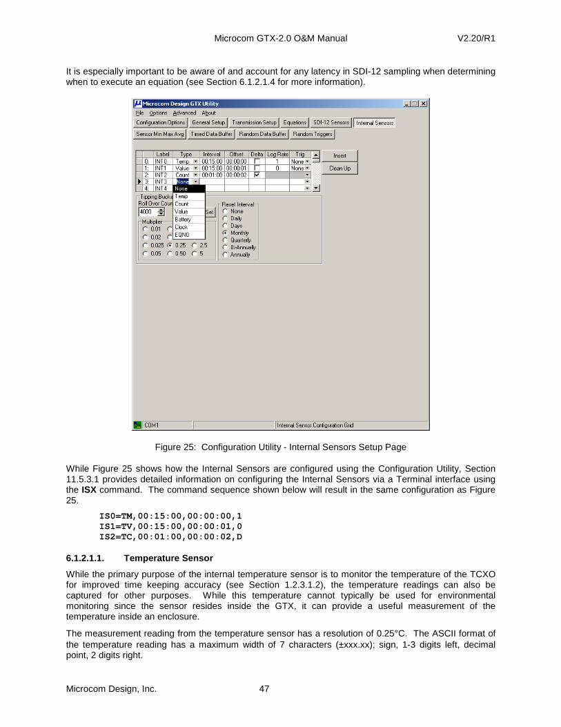
Microcom GTX-2.0 O&M Manual V2.20/R1
Microcom Design, Inc. 47
It is especially important to be aware of and account for any latency in SDI-12 sampling when determining when to execute an equation (see Section 6.1.2.1.4 for more information).
Figure 25: Configuration Utility - Internal Sensors Setup Page
While Figure 25 shows how the Internal Sensors are configured using the Configuration Utility, Section 11.5.3.1 provides detailed information on configuring the Internal Sensors via a Terminal interface using the ISX command. The command sequence shown below will result in the same configuration as Figure 25.
IS0=TM,00:15:00,00:00:00,1 IS1=TV,00:15:00,00:00:01,0 IS2=TC,00:01:00,00:00:02,D
6.1.2.1.1. Temperature Sensor
While the primary purpose of the internal temperature sensor is to monitor the temperature of the TCXO for improved time keeping accuracy (see Section 1.2.3.1.2), the temperature readings can also be captured for other purposes. While this temperature cannot typically be used for environmental monitoring since the sensor resides inside the GTX, it can provide a useful measurement of the temperature inside an enclosure.
The measurement reading from the temperature sensor has a resolution of 0.25°C. The ASCII format of the temperature reading has a maximum width of 7 characters (±xxx.xx); sign, 1-3 digits left, decimal point, 2 digits right.

Microcom GTX-2.0 O&M Manual V2.20/R1
Microcom Design, Inc. 48
6.1.2.1.2. Tipping Bucket Counter
The tipping bucket counter interface allows connection to industry standard contact-closure style tipping buckets for measuring rainfall accumulation (see Section 2.1.3). The counter increments every time it detects a switch contact closure from the tipping bucket; each tip is calibrated to a predetermined amount of rainfall.
The tipping bucket counts can be collected periodically and transmitted to provide an indication of the amount of rainfall that has occurred at a remote site. The rainfall measurement can be collected as raw counts or as a scaled value. Scaling allows the rainfall value to be reported in engineering units (e.g. inches or millimeters).
The tipping bucket counter can be automatically cleared (reset to 0) on a variety of schedules or simply allowed to rollover at a user defined terminal value. The counter resolution is 16-bits, which yields a count range of 0 to 65,535.
The ASCII format of the tipping bucket counts is an integer value with leading 0 digits; the number of digits is equal to the number of digits in the terminal count minus one. For example, for a roll over count of 1001-10000, the tipping bucket count will always be reported with four digits (e.g. 0000); for terminal counts greater than 9999 (i.e. 10001-65535), the counts will be reported with five digits (e.g. 00000).
6.1.2.1.2.1. Tipping Bucket Scaling
As shown in Figure 25, the Tipping Bucket Multiplier can be set to one of 12 standard values; the default value is 1. When scaling is active (not set to 1), the tipping bucket value will be the scaled product of the Multiplier times the raw counts. See Section 11.5.3.10 for information on using the Terminal command (TBM) to set this value.
The ASCII format of the Tipping Bucket Value depends on both the rollover limit and the scaling multiplier, and includes leading zeroes, if necessary. The number of decimal places (digits to the right of the decimal point) will be the same as the multiplier. Further, since the value is reported with leading 0 digits; the number of digits to the left of the decimal point can be determined by computing the maximum value. For example, if the rollover count set to 4000 with a Multiplier of 0.25, the maximum reading is 999.75 (0.25*(4000-1)). Accordingly, for this example, the value will be between 000.00 and 999.75, inclusive. Figure 29 shows another example for this configuration.
6.1.2.1.2.2. Tipping Bucket Rollover
The user can define a rollover value for the tipping bucket raw counts to limit the range of the counts and/or the Tipping Bucket Value. As shown in Figure 25 and Figure 29, this value is entered in the edit box in the “Tipping Bucket Setup” group. The maximum reading for the counts is 1 less than the rollover count, i.e. the counter rolls back to 0 when it would equal this number. Setting the rollover to 0 allows the counter to reach the maximum 16-bit value of 65,535. See Section 11.5.3.11 for information on using the Terminal command (TBR) to set this parameter.
6.1.2.1.2.3. Tipping Bucket Auto Clear
The GTX can be configured to automatically clear the counter on one of the time schedules shown in Figure 25 (e.g. Monthly). When the internal clock advances the day, it checks the Reset Interval and zeroes the counter if necessary. The Reset Interval can be a fixed number of days or can be scheduled to coincide with the 1ST of the month. Setting the Reset Interval to Monthly (Jan-Dec), Quarterly (Jan, Apr, Jul, Oct), Bi-Annually (Jan, Jul), or Annually (Jan) will reset on the first of the months listed parenthetically. See Section 11.5.3.12 for information on using the Terminal interface to configure the Reset Interval using the TBA command.
When the “Daily” auto clear option is selected, the user can also specify a precise UTC hour as to when to clear the tipping bucket as shown in Figure 26. The default value is hour 0, i.e. at the beginning of the new UTC day, but allowing the hour to be specified can be useful to have the reset occur at the start of the local day.
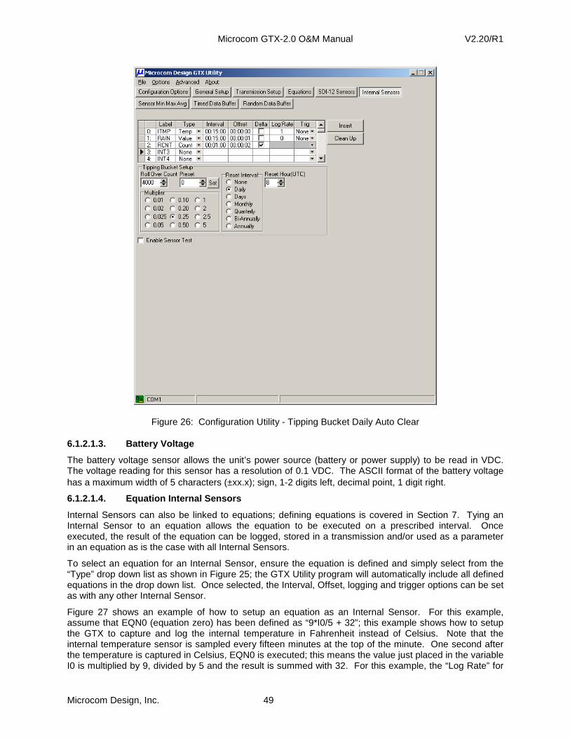
Microcom GTX-2.0 O&M Manual V2.20/R1
Microcom Design, Inc. 49
Figure 26: Configuration Utility - Tipping Bucket Daily Auto Clear
6.1.2.1.3. Battery Voltage
The battery voltage sensor allows the unit’s power source (battery or power supply) to be read in VDC. The voltage reading for this sensor has a resolution of 0.1 VDC. The ASCII format of the battery voltage has a maximum width of 5 characters (±xx.x); sign, 1-2 digits left, decimal point, 1 digit right.
6.1.2.1.4. Equation Internal Sensors
Internal Sensors can also be linked to equations; defining equations is covered in Section 7. Tying an Internal Sensor to an equation allows the equation to be executed on a prescribed interval. Once executed, the result of the equation can be logged, stored in a transmission and/or used as a parameter in an equation as is the case with all Internal Sensors.
To select an equation for an Internal Sensor, ensure the equation is defined and simply select from the “Type” drop down list as shown in Figure 25; the GTX Utility program will automatically include all defined equations in the drop down list. Once selected, the Interval, Offset, logging and trigger options can be set as with any other Internal Sensor.
Figure 27 shows an example of how to setup an equation as an Internal Sensor. For this example, assume that EQN0 (equation zero) has been defined as “9*I0/5 + 32”; this example shows how to setup the GTX to capture and log the internal temperature in Fahrenheit instead of Celsius. Note that the internal temperature sensor is sampled every fifteen minutes at the top of the minute. One second after the temperature is captured in Celsius, EQN0 is executed; this means the value just placed in the variable I0 is multiplied by 9, divided by 5 and the result is summed with 32. For this example, the “Log Rate” for

Microcom GTX-2.0 O&M Manual V2.20/R1
Microcom Design, Inc. 50
INT0 has been set to 0, disabling the logging of the Celsius, and the “Log Rate” for INT3 is set to 1, enabling the capture of the internal GTX temperature in Fahrenheit in the data log.
Figure 27: Configuration Utility - Equation Internal Sensor Setup
As noted above, it is important to properly schedule the execution of an equation relative to the sampling of the sensor values that are to be used in the equation to ensure the correct and most current values are utilized in the calculations. While the latency in sampling the GTX’s Internal Sensors is negligible (i.e. equations can be executed within a second of the Internal Sensor sampling), SDI-12 Sensors can have a considerable time delay (several seconds to even minutes) between the request to perform the sample and when the reading is available to be collected. These time delays must be accounted for when scheduling equations that operate on SDI-12 Sensor values.
For example assume, and SDI-12 sensor is sampled every 10 minutes with an offset of 00:00:00 (i.e. at xx:10:00, xx:20:00, and so on). Further, assume the particular SDI-12 sensor requires 5 seconds to complete the measurement before the reading is available and that an equation is required to process the sampled value. In this example, the equation should be scheduled to execute every ten minutes with an offset of at least 00:00:06 (six seconds) to be certain the latest sample is available for when the equation executes.

Microcom GTX-2.0 O&M Manual V2.20/R1
Microcom Design, Inc. 51
6.1.2.1.5. Clock Internal Sensors
Selecting a “Clock” internal sensor allows the GTX’s internal clock to be sampled and captured. The captured value can then be used to place a timestamp in a transmission before and/or be used in a calculation.
As shown in Figure 28, once the Internal Sensor “Type” is set to “Clock”, the “Delta” and “Log Rate” rate fields are disabled, i.e. clock samples cannot be logged – there’s no reason to log a clock value since all logged parameters and events automatically include a timestamp. For a “Clock” Internal Sensor, the “Trig” cell drop down list is populated with a series of time/date formatting options that are used to select the desired format for the clock sample.
Figure 28: Configuration Utility - Clock Internal Sensor Setup
One of thirty-three different formatting strings are available that allow capturing and formatting various subsets of the GTX’s date and time fields (i.e. secs, minutes, hours, day, month, year). The formatting options are summarized in Table 11. As the table indicates, time/date strings can be generated with or without the standard separators (colon for time and slash for date). All fields are generated with leading zeroes, where applicable, and the year field is always four digits.
If the Clock Internal Sensor is selected to be in an ASCII formatted transmission buffer, the field width must be sufficient to accommodate the data and separators if specified. When used in a Pseudo Binary transmission buffer or in an equation, the value of the clock sensor is simply the numeric value of the digits up to the first separator character, if present.

Microcom GTX-2.0 O&M Manual V2.20/R1
Microcom Design, Inc. 52
Format String
Field(s)
Example Output 01/02/2013 12:34:56
Sensor Value
S Second 56 56 MI Minute 34 34 MS Minute, Second 3456 3456 M:S Minute, Second 34:56 34 H Hour 12 12
HM Hour, Minute 1234 1234 H:M Hour, Minute 12:34 12 HMS Hour, Minute, Second 123456 123456 H:M:S Hour, Minute, Second 12:34:56 12 JHMS Julian Day, Hour, Minute, Second 002123456 002123456
J:H:M:S Julian Day, Hour, Minute, Second 002:12:34:56 002 D Day of Month 02 02
MO Month 01 01 Y Year 2013 2013 J Julian Day 002 002
MD Month, Day of Month 0102 0102 M/D Month, Day of Month 01/02 01 MDY Month, Day of Month, Year 01022013 01022013 M/D/Y Month, Day of Month, Year 01/02/2013 01
DM Day of Month, Month 0201 0201 D/M Day of Month, Month 02/01 02 DMY Day of Month, Month, Year 02012013 02012013 D/M/Y Day of Month, Month, Year 02/01/2013 02
MY Month, Year 012013 012013 M/Y Month, Year 01/2013 01 YM Year, Month 201301 201301 Y/M Year, Month 2013/01 2013 YMD Year, Month, Day of Month 20130102 20130102 Y/M/D Year, Month, Day of Month 2013/01/02 2013
JY Julian Day, Year 0022013 0022013 J/Y Julian Day, Year 002/2013 002 YJ Year, Julian Day 2013002 2013002 Y/J Year, Julian Day 2013/002 2013
Table 11: Clock Internal Sensor Formats and Values
6.1.2.1.6. Testing the Internal Sensors
Figure 29 shows the Internal Sensor page of the Configuration Utility when it is in the Configure/Control/Deploy GTX modes (see Section 3.2.4). In this mode, the utility provides access to “Enable Sensor Test”. Further, to display the “Tests” group, the “Enable Sensor Test” box must be checked as shown.
The Temperature, Bucket Count, Bucket Value, and Battery Voltage buttons can be used to read the current sensor values. These buttons are equivalent to issuing the TOT? (Section 11.5.3.7), TBC? (Section 11.5.3.8), TBV? (Section 11.5.3.9), and RBV? (Section 11.10.17) commands, respectively.
Selecting a row where the Internal Sensor is tied to an equation then clicking the “Equation Test” button will direct the GTX to execute the associated equation. In the example below, EQN0 is defined to convert the temperature reading from Celsius to Fahrenheit. While equations are defined in standard Infix notation (see Section 7), the actual process of the equation execution is shown in Postfix notation where the operands follow the operators (this is also known as Reverse Polish Notation or RPN).
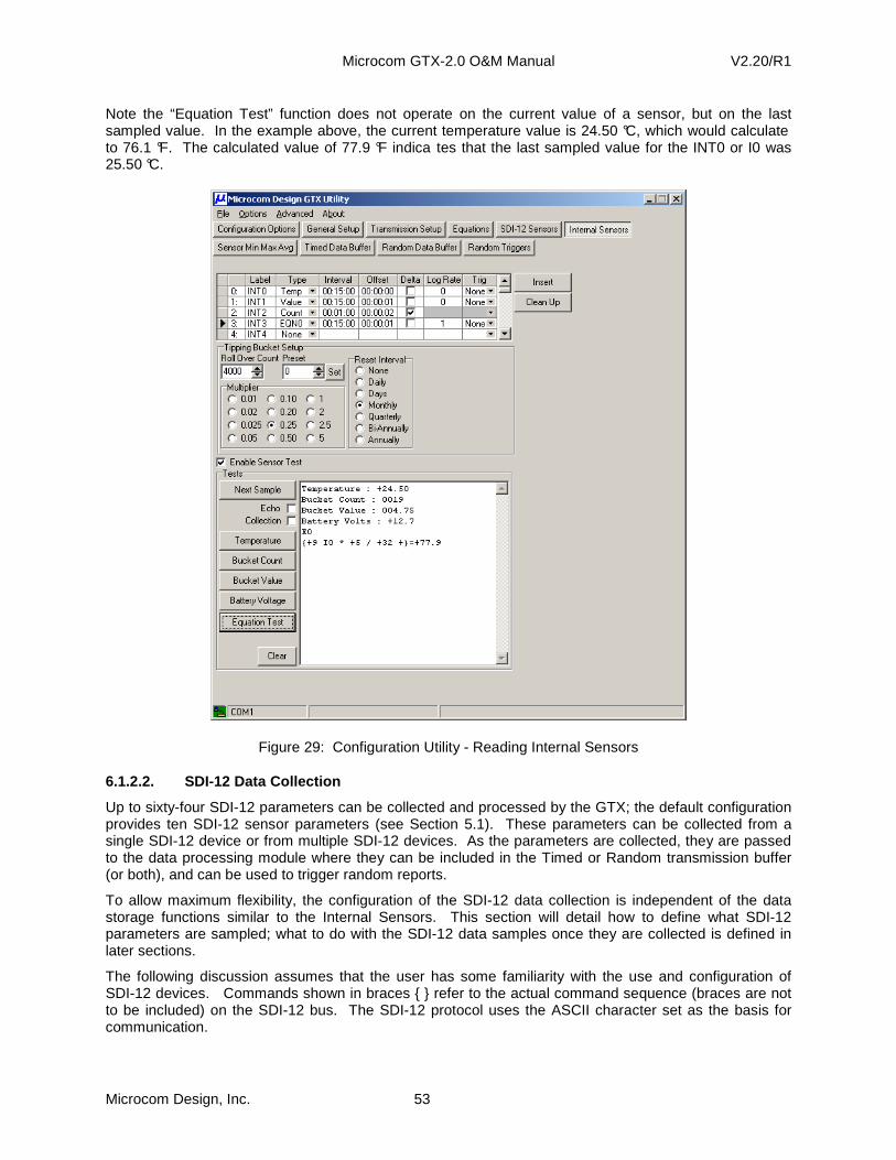
Microcom GTX-2.0 O&M Manual V2.20/R1
Microcom Design, Inc. 53
Note the “Equation Test” function does not operate on the current value of a sensor, but on the last sampled value. In the example above, the current temperature value is 24.50 °C, which would calculate to 76.1 °F. The calculated value of 77.9 °F indica tes that the last sampled value for the INT0 or I0 was 25.50 °C.
Figure 29: Configuration Utility - Reading Internal Sensors
6.1.2.2. SDI-12 Data Collection
Up to sixty-four SDI-12 parameters can be collected and processed by the GTX; the default configuration provides ten SDI-12 sensor parameters (see Section 5.1). These parameters can be collected from a single SDI-12 device or from multiple SDI-12 devices. As the parameters are collected, they are passed to the data processing module where they can be included in the Timed or Random transmission buffer (or both), and can be used to trigger random reports.
To allow maximum flexibility, the configuration of the SDI-12 data collection is independent of the data storage functions similar to the Internal Sensors. This section will detail how to define what SDI-12 parameters are sampled; what to do with the SDI-12 data samples once they are collected is defined in later sections.
The following discussion assumes that the user has some familiarity with the use and configuration of SDI-12 devices. Commands shown in braces { } refer to the actual command sequence (braces are not to be included) on the SDI-12 bus. The SDI-12 protocol uses the ASCII character set as the basis for communication.
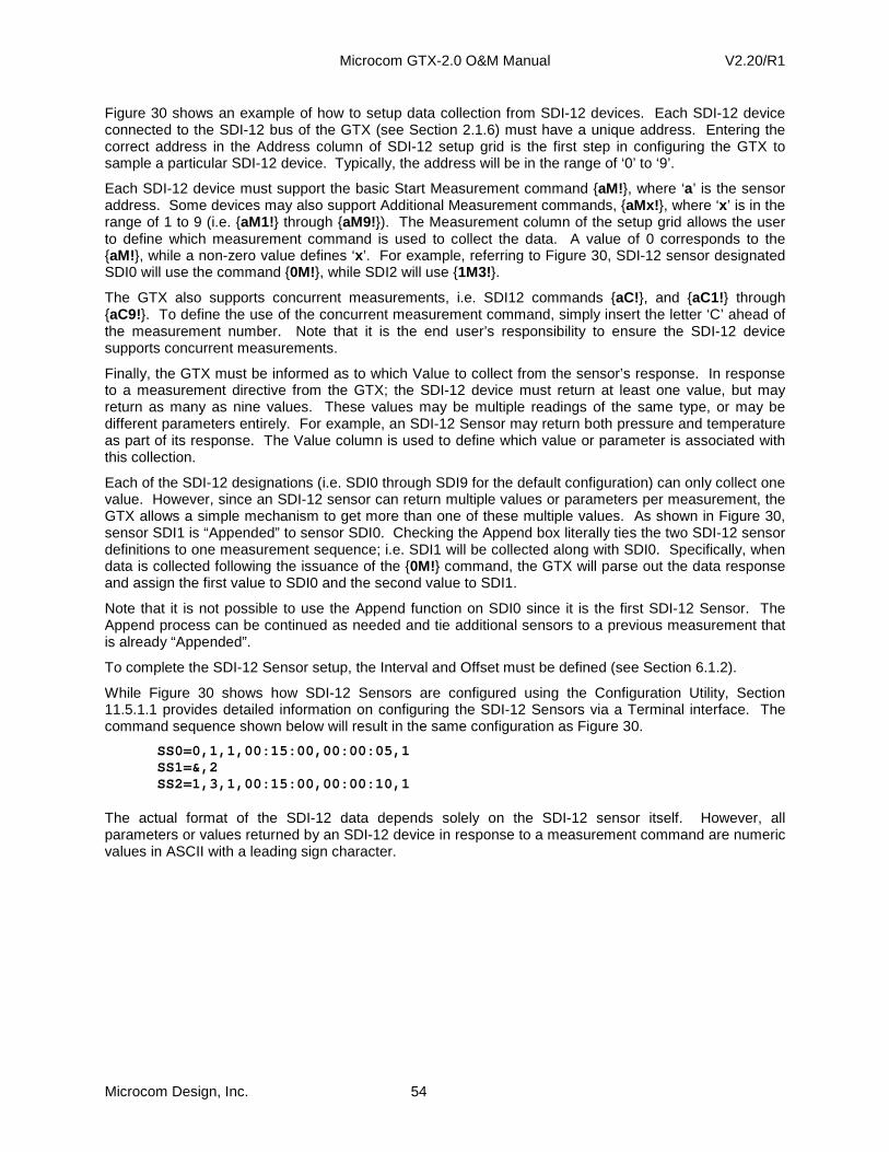
Microcom GTX-2.0 O&M Manual V2.20/R1
Microcom Design, Inc. 54
Figure 30 shows an example of how to setup data collection from SDI-12 devices. Each SDI-12 device connected to the SDI-12 bus of the GTX (see Section 2.1.6) must have a unique address. Entering the correct address in the Address column of SDI-12 setup grid is the first step in configuring the GTX to sample a particular SDI-12 device. Typically, the address will be in the range of ‘0’ to ‘9’.
Each SDI-12 device must support the basic Start Measurement command {aM!}, where ‘a’ is the sensor address. Some devices may also support Additional Measurement commands, {aMx!}, where ‘x ’ is in the range of 1 to 9 (i.e. {aM1!} through {aM9!}). The Measurement column of the setup grid allows the user to define which measurement command is used to collect the data. A value of 0 corresponds to the {aM!}, while a non-zero value defines ‘x’. For example, referring to Figure 30, SDI-12 sensor designated SDI0 will use the command {0M!}, while SDI2 will use {1M3!}.
The GTX also supports concurrent measurements, i.e. SDI12 commands {aC!}, and {aC1!} through {aC9!}. To define the use of the concurrent measurement command, simply insert the letter ‘C’ ahead of the measurement number. Note that it is the end user’s responsibility to ensure the SDI-12 device supports concurrent measurements.
Finally, the GTX must be informed as to which Value to collect from the sensor’s response. In response to a measurement directive from the GTX; the SDI-12 device must return at least one value, but may return as many as nine values. These values may be multiple readings of the same type, or may be different parameters entirely. For example, an SDI-12 Sensor may return both pressure and temperature as part of its response. The Value column is used to define which value or parameter is associated with this collection.
Each of the SDI-12 designations (i.e. SDI0 through SDI9 for the default configuration) can only collect one value. However, since an SDI-12 sensor can return multiple values or parameters per measurement, the GTX allows a simple mechanism to get more than one of these multiple values. As shown in Figure 30, sensor SDI1 is “Appended” to sensor SDI0. Checking the Append box literally ties the two SDI-12 sensor definitions to one measurement sequence; i.e. SDI1 will be collected along with SDI0. Specifically, when data is collected following the issuance of the {0M!} command, the GTX will parse out the data response and assign the first value to SDI0 and the second value to SDI1.
Note that it is not possible to use the Append function on SDI0 since it is the first SDI-12 Sensor. The Append process can be continued as needed and tie additional sensors to a previous measurement that is already “Appended”.
To complete the SDI-12 Sensor setup, the Interval and Offset must be defined (see Section 6.1.2).
While Figure 30 shows how SDI-12 Sensors are configured using the Configuration Utility, Section 11.5.1.1 provides detailed information on configuring the SDI-12 Sensors via a Terminal interface. The command sequence shown below will result in the same configuration as Figure 30.
SS0=0,1,1,00:15:00,00:00:05,1 SS1=&,2 SS2=1,3,1,00:15:00,00:00:10,1
The actual format of the SDI-12 data depends solely on the SDI-12 sensor itself. However, all parameters or values returned by an SDI-12 device in response to a measurement command are numeric values in ASCII with a leading sign character.

Microcom GTX-2.0 O&M Manual V2.20/R1
Microcom Design, Inc. 55
Figure 30: Configuration Utility - SDI-12 Sensors Setup Page
6.1.3. SDI-12 Power Control
As shown in Figure 30, the bottom of the SDI-12 Sensors setup page also includes several controls that are used to define when the SDI-12 Power bus is enabled. The “GTX Enabled” group box in the “SDI-12 Power” section is used to define how the SDI-12 Power should be controlled when the unit is enabled; the three options are “Always Off”, “Always On”, and “On Per Schedule”. The “GTX Disabled” group box defines what the SDI-12 Power should do when the GTX is disabled; the only option here are “Always Off” or “Always On”. Note that the default settings for both these group boxes are “Always On”, i.e. the SDI-12 Power is always present.
When the GTX is configured for “On Per Schedule”, the table in the center of the “SDI-12 Power” section is used to define the On/Off schedule. Up to six schedules (0 thru 5) can be defined allowing for multiple distinct on times, as well as for overlapping on times.
For each entry in the table, three fields are defined; an interval, an offset, and a duration. The interval and offset settings operate in a similar fashion to the rate intervals and offsets for sensor sampling. Specifically, the interval determines how often the power should be turned on and the offset determines where within the interval the power should be turned on. The duration determines how long the SDI-12 power should be on. In the table, all three fields are specified in “hh:mm:ss” format.
The offset and duration values must be strictly less than the interval. The interval and duration values cannot be zero; except in the case where all three values are zero which is an undefined or cleared entry. The minimum interval is 15 seconds and the maximum interval is twenty-four hours (i.e. 24:00:00).

Microcom GTX-2.0 O&M Manual V2.20/R1
Microcom Design, Inc. 56
The ability to turn SDI-12 supply off and on can be useful to reduce the overall system power requirements by only powering up SDI-12 devices when necessary to make measurements. Note that this feature should not be used with sensors that provide average (e.g. average wind speed) or accumulated (e.g. rainfall) readings since the sensor will not be able make the necessary measurements to update averages or accumulate totals during the time the SDI-12 bus is powered down. Further, when programming the SDI-12 Power On/Off cycle, consideration must be given to warm-up times required by the SDI-12 sensors.
While the SDI-12 Power is primarily intended for the SDI-12 bus, this switchable +12 VDC output can be used to power other devices as well, and the programmable on/off features can be used to only enable these devices when necessary. The only requirement is that total maximum current for all devices be limited to 0.5 amps; the +12V supply for the SDI-12 bus has an inline self-resetting fuse of 1 amp.
Figure 31 shows an example of SDI-12 Power scheduling. In this example, the first three schedules in the table are defined, and the last three are unused (i.e. “Interval”, “Offset”, and “Duration all “00:00:00”). Note that for the schedule to be active, the “GTX Enabled” setting MUST be set to “On Per Schedule”. This separate control setting is useful when it is desired to disable the On/Off schedule without having to clear the table values.
Figure 31: Configuration Utility - SDI-12 Power Schedule Example
In the example shown in Figure 31, the first entry will result in the SDI-12 Power coming on every fifteen minutes at 7 minutes into the interval (i.e. at xx:07:00, xx:22:00, xx:37:00, and xx:52:00), and will be on for two minutes (i.e. until xx:09:00, xx:24:00, xx:39:00, and xx:54:00). The second entry adds an
Microcom GTX-2.0 O&M Manual V2.20/R1
Microcom Design, Inc. 57
additional point in time where the SDI-12 bus will be powered up for 30 seconds before the top of each hour and stay on until 30 seconds after the hour (1 minute in total). The third table entry defines an overlapping segment where the SDI-12 Power will be for an entire hour every day beginning at 12:00:00 UTC.
As this example shows, the ability to define multiple entries in the SDI-12 Power table allows for several distinct and/or overlapping regions. If any entry in the table indicates the SDI-12 Power should be on, then the SDI-12 bus will be powered. Only when all entries in the table indicate that the SDI-12 Power should be off will the power be removed from the SDI-12 bus.
Section 11.5.2, details how to define the SDI-12 Power controls using the Terminal interface. Note that the “On Per Schedule” option in the “GTX Enabled” group box is equivalent to the Auto mode when using the terminal commands to define the SDI-12 Power Mode (see Section 11.5.2.2).
6.1.4. Sensor Data Logging
As shown in Figure 25 and Figure 30, both Internal and SDI-12 Sensors have Log Rate, Delta, and Trig columns. As has been noted previously, the data collected can also be logged to a nonvolatile Data/Event buffer. Each logged data point has its own timestamp.
In a typical DCP application, data is being continuously sampled, buffered and transmitted in “near real-time”. As long as the data is properly received, this “near real-time” data can be used for rapid response to changing environmental conditions. However, this data can also be archived for historical analysis.
As long as the communication link is unobstructed, the received data will be readily and reliably available for both types of use. However, if a fault condition (e.g. a broken antenna cable) disrupts the link, the data is irretrievably lost for the “near real-time” application. On the other hand, the ability to log and retrieve data ensures that gaps in the historical archive can be filled in at a later date. This ability also allows the GTX to operate in a Logger only mode.
While the default is to log all data values collected, the GTX provides a mechanism to maximize the historical length of the log. In the “near real-time” application, it’s quite often necessary to have several data points collected within an hour for a particular sensor. However, archiving this much data may not be practical, or simply not required. For example, it may be desirable to have 15 minute data points collected and transmitted, but only the hourly readings archived. This simple example reduces the memory requirements by a factor of 4. This memory reduction directly translates into a factor of 4 increase in the archival capabilities of the GTX log. For example, instead of one month worth of data being logged, four months would be saved; or instead of 3 months, a full year could be retrieved.
Reducing the logging rate will also reduce the time to retrieve a block of data.
Accordingly, both the Internal and SDI-12 Sensor configurations allow each sensor’s data to be logged at a multiple of the sampling rate. As noted previously, the default Log Rate is 1, i.e. every sample is saved. If the Log Rate values in Figure 25 and Figure 30, are changed from 1 to 4, then only an hourly sample is stored in the log.
The product of the Log Rate and the Interval, effectively defines a “Logging Interval”. Further, the GTX automatically determines a similar, relative “Logging Offset” to ensure the saved sample is at a specific and determinable time. Continuing the previous example and assuming the Offset is 00:00:00, the GTX does not simply log every fourth reading beginning whenever the unit is Enabled, instead it will ensure that the top of the hour readings are saved. If the Log Rate is reduced to 2, samples will be saved ON the half hour; if the Log Rate is increased to 96 (4*24), then the data point will be logged at midnight.
The GTX also allows the user to define two logging modifier flags, ‘H’ and ‘L’. These flags, when set, direct the GTX to log all sample points from this sensor when the value is above or below a Random Trigger Limit for this sensor. Specifically, if the defined sensor is used as a High or Rise random/sensor trigger and the current reading is above either of these thresholds, the value will be logged regardless of the log interval. If the defined sensor is used as a Low or Fall random/sensor trigger and the current reading is below either of these thresholds, the value will also be logged independent of the log interval.
This mechanism allows data to be logged more frequently when conditions warrant, and less frequently otherwise. A special “Log Only” version the Random Report Triggers can also be defined so that the

Microcom GTX-2.0 O&M Manual V2.20/R1
Microcom Design, Inc. 58
trigger mechanism applies just to the logging of the sensor, i.e. it will not trigger a random report. See Sections 9.5, 9.6, and 11.7.5 for information on Random Report Triggers.
Figure 32 shows how to set these flags using the Configuration Utility. Selecting “High” only enables the ‘H’ flag; selecting “Low” only enables the ‘L’ flag; selecting “H/L” enables both and “None” disables all three.
Random triggers can also be defined as Delta, i.e. the trigger occurs when the difference between the current and the last value is above/below a specified limit. Logging can also be based on these Delta triggers. In the High case, the logging will be done when the difference value is above the positive limit, i.e. the rate of change is in the positive direction and exceeds the threshold. For the Low log trigger, data will only be collected when the difference between the current and the last value is below the negative value of the limit, i.e. the rate of change is in the negative direction and exceeds the threshold.
Figure 32: Configuration Utility - Setting Logging Trigger Flags
Another option provided by the GTX is Delta logging. As shown in Figure 32, checking the Delta box disables the Log Rate and Trig fields, and enables the Delta logging feature. Delta logging directs the GTX to only save a new value when it is different from the previously stored value. This can be a highly effective approach for data such as a Tipping Bucket Rain-gauge, where for extended periods of time the data does not change at all (e.g. it has not rained). Using this approach, collected data can be sampled at much higher rates and logged with finer resolution when an event is occurring (e.g. when its raining) without overtaxing the memory storage.
For example, Figure 32 has the tipping bucket count being sampled on a one-minute basis, but a data point is only logged when the new sample is different from the previously stored value. If each an every data point were save, the log would have 1,440 points per day; if it didn’t rain during the day, this would mean 1,440 points with exactly the same value would be stored! However, when it is raining, data is sampled and stored much more frequently than it is collected for transmission (e.g. every 15 minutes). This added resolution in sampling not only provides more precise timing to better determine when it actually rained; it also provides an indication of how hard it rained.
As shown in Figure 25, the Log Rate can also be set to 0, which will disable logging for this sensor. For the example shown, the Tipping Bucket Value is redundant since the Tipping Bucket Count is being saved.
6.1.5. Sensor Labeling
The figures shown throughout this section have utilized the default Labels for the Internal (INTx or INxx) and the SDI-12 (SDIx or SDxx) Sensors. The GTX, and therefore the Configuration Utility, also allows the user to redefine these the labels. By placing the cursor in the desired Label field, the user can overwrite the existing designator with any 1-4 character string.
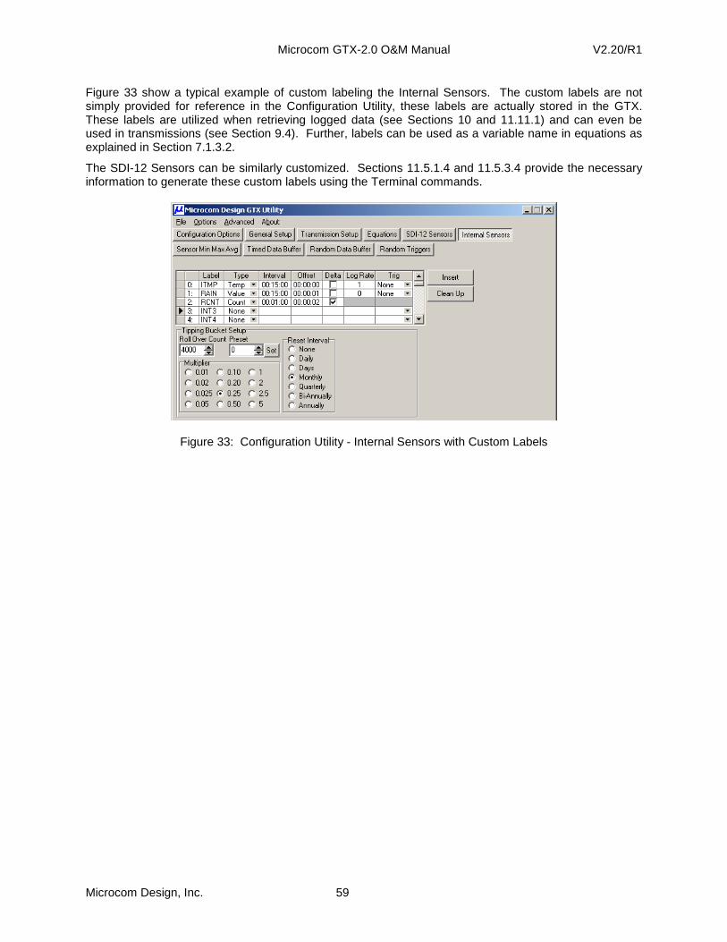
Microcom GTX-2.0 O&M Manual V2.20/R1
Microcom Design, Inc. 59
Figure 33 show a typical example of custom labeling the Internal Sensors. The custom labels are not simply provided for reference in the Configuration Utility, these labels are actually stored in the GTX. These labels are utilized when retrieving logged data (see Sections 10 and 11.11.1) and can even be used in transmissions (see Section 9.4). Further, labels can be used as a variable name in equations as explained in Section 7.1.3.2.
The SDI-12 Sensors can be similarly customized. Sections 11.5.1.4 and 11.5.3.4 provide the necessary information to generate these custom labels using the Terminal commands.
Figure 33: Configuration Utility - Internal Sensors with Custom Labels

Microcom GTX-2.0 O&M Manual V2.20/R1
Microcom Design, Inc. 60
7. Equation Processor
The Microcom GTX-2.0 incorporates a powerful, yet easy to use, Equation Processor to allow the user to numerically manipulate acquired data in virtually unlimited ways. Equations are defined and scheduled independently of the sampled sensors they operate on. Further, an equation may consist of a single evaluation or may have multiple evaluations strung together that are executed in left-to-right order. The ability to combine multiple evaluations in a single equation provides the user ability to define a subroutine to be executed.
Once an equation is defined, it can be attached to an Internal Sensor, which allows the evaluation to be scheduled exactly like any other sensor. Likewise, the end result of the equation is essentially a new “sensor sample” that can be further processed just like an actual sensor value. In other words, the equation result can be stored in the Data/Event log, passed on to a Min, Max, Average Processor (see Section 8), stored in a transmission buffer, used to trigger a Random report, and/or used in a subsequent equation.
Equations can be used to provide simple data conversion; such as, converting a sensor from one engineering unit to another, or altering the data precision (adding or removing decimal places for formatting).
Equations can also be used to provide complex data manipulation such as polynomial curve fitting or spatial manipulation (combining or averaging multiple sensor readings to produce a single result). By properly scheduling multiple equations and other processes, even relatively complex tasks such as producing composite time averages and min/max functions can be readily accomplished. Note that the Min, Max, Average (MMA) Processor covered in Section 8 allows these operations on a single value; by combining these processes with the proper scheduling, MMA values can be acquired for the results of more complex manipulation of collected data.
Equations can even be used to extend the log/sampling ratios for sensors. The GTX logging function operates as a multiple of sensor samples, but is limited to a log/sample ratio of 250; i.e. for a given sampling interval, the maximum delay in logged values is limited to 250. With this limit, logging a sensor once a day requires a minimum sampling interval of 6 minutes (6*240 = 1,440 minutes = 24 hours). By using an equation to simply capture a sensor value (i.e. assign the sensor reading as the equation result), the log/sample ratio can be easily extended. To accomplish this the sensor reading is not directly logged instead, the equation is defined to extract the value at the desired log rate and the equation value can be logged. Note that the actual sensor sample provided at this rapid rate can still be used for all other processes (e.g. MMA result, Random triggering, etc.).
7.1. Equation Basics
Equations are defined by the user as ASCII strings. The equations strings are stored in the GTX’s soft configuration memory, and are recalled based on a user defined schedule (as defined by the Internal Sensor schedule the equation is tied to). Once recalled, the equation is then parsed and executed.
7.1.1. Equation Operators
Permissible equation operators are provided in Table 12 below. As indicated in Table 12, the GTX supports all major numerical functions (add, sub, multiply, etc.), as well as, the standard relational functions (equal to, not equal to, greater than, etc.). As also indicated, parenthesis are supported to override operator precedence where necessary.
The GTX also supports the exponent operator (^), which allows polynomial equations to be executed for curve fitting, and fractional roots (e.g. I0^0.5 takes the square root of I0).
Note that the Assignment operator and the Equal To operator are both a single equals sign. The GTX will only accept an equal sign as the assignment operator when it immediately follows a single variable at the start of the equation; otherwise, the GTX assumes the equals sign is the Equal To operator. For example, “I0=10 …” is an assignment operation; “(I0=10) …” and “10=I0 …” are Equal To operators.
The If-Construct operator (?), allows the user to easily enter conditional equations. The use of the If-Construct is covered in detail in Section 7.4.
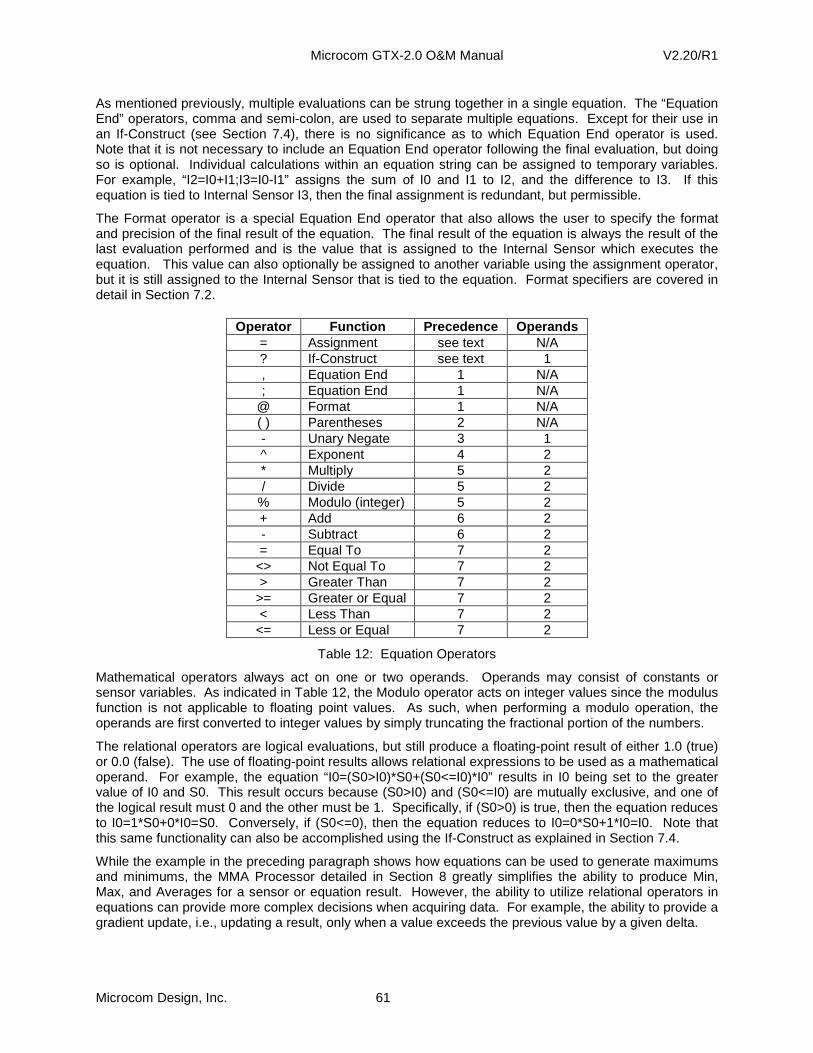
Microcom GTX-2.0 O&M Manual V2.20/R1
Microcom Design, Inc. 61
As mentioned previously, multiple evaluations can be strung together in a single equation. The “Equation End” operators, comma and semi-colon, are used to separate multiple equations. Except for their use in an If-Construct (see Section 7.4), there is no significance as to which Equation End operator is used. Note that it is not necessary to include an Equation End operator following the final evaluation, but doing so is optional. Individual calculations within an equation string can be assigned to temporary variables. For example, “I2=I0+I1;I3=I0-I1” assigns the sum of I0 and I1 to I2, and the difference to I3. If this equation is tied to Internal Sensor I3, then the final assignment is redundant, but permissible.
The Format operator is a special Equation End operator that also allows the user to specify the format and precision of the final result of the equation. The final result of the equation is always the result of the last evaluation performed and is the value that is assigned to the Internal Sensor which executes the equation. This value can also optionally be assigned to another variable using the assignment operator, but it is still assigned to the Internal Sensor that is tied to the equation. Format specifiers are covered in detail in Section 7.2.
Operator Function Precedence Operands = Assignment see text N/A ? If-Construct see text 1 , Equation End 1 N/A ; Equation End 1 N/A
@ Format 1 N/A ( ) Parentheses 2 N/A - Unary Negate 3 1 ^ Exponent 4 2 * Multiply 5 2 / Divide 5 2
% Modulo (integer) 5 2 + Add 6 2 - Subtract 6 2 = Equal To 7 2
<> Not Equal To 7 2 > Greater Than 7 2
>= Greater or Equal 7 2 < Less Than 7 2
<= Less or Equal 7 2
Table 12: Equation Operators
Mathematical operators always act on one or two operands. Operands may consist of constants or sensor variables. As indicated in Table 12, the Modulo operator acts on integer values since the modulus function is not applicable to floating point values. As such, when performing a modulo operation, the operands are first converted to integer values by simply truncating the fractional portion of the numbers.
The relational operators are logical evaluations, but still produce a floating-point result of either 1.0 (true) or 0.0 (false). The use of floating-point results allows relational expressions to be used as a mathematical operand. For example, the equation “I0=(S0>I0)*S0+(S0<=I0)*I0” results in I0 being set to the greater value of I0 and S0. This result occurs because (S0>I0) and (S0<=I0) are mutually exclusive, and one of the logical result must 0 and the other must be 1. Specifically, if (S0>0) is true, then the equation reduces to I0=1*S0+0*I0=S0. Conversely, if (S0<=0), then the equation reduces to I0=0*S0+1*I0=I0. Note that this same functionality can also be accomplished using the If-Construct as explained in Section 7.4.
While the example in the preceding paragraph shows how equations can be used to generate maximums and minimums, the MMA Processor detailed in Section 8 greatly simplifies the ability to produce Min, Max, and Averages for a sensor or equation result. However, the ability to utilize relational operators in equations can provide more complex decisions when acquiring data. For example, the ability to provide a gradient update, i.e., updating a result, only when a value exceeds the previous value by a given delta.
Microcom GTX-2.0 O&M Manual V2.20/R1
Microcom Design, Inc. 62
7.1.2. Equation Constants
Equation constants can be defined inline as standard numerical values or can utilize one of up to sixty-four special configurable constants, designated as K0 through K63. Inline constants simplify the equation definition process, but cannot be altered without redefining the equation, which requires disabling the GTX. Alternately, special provisions in the GTX code allow configuration constants to be modified while the GTX is enabled. This implementation allows these configurable constants to be altered, which in essence allows the equation to be modified, even though the GTX is enabled.
Configuration constants are especially useful when it is necessary or desirable to apply calibration factors or offsets to a sensor reading. Using configuration constants to perform calibration corrections allows the calibration constants to be tweaked without having to stop normal GTX operations. Further, when a configurable constant (K0-K63) is changed when the GTX is enabled, the change is captured as an Event in the Data/Event Log providing a record of any “calibration” changes.
7.1.2.1. Inline Constants
Inline constants are simply numerical values defined in the equation string (e.g. 3.141593). Constants can be entered with any number of significant digits and can use the exponent designation, E, (e.g. 1E5 = 105). However, the GTX’s mathematical functions are performed in single precision IEEE 4-byte floating-point format. As such, constants, intermediate results, and the final result have an inherent precision of 7 significant digits.
7.1.2.2. Configuration Constants
As mentioned above, a special class of constants is also available for use in equations that are stored as part of the soft configuration memory. A unique feature of the constants is that the “constant value” can be modified even while the GTX is enabled. Up to 64 configurable equation constants can be defined and are designated K0 through K63. Initially these equation constants default to a value of zero, but can be initialized as part of the GTX configuration.
Since configuration constants are changeable while the GTX is in operation, they are especially useful for applying calibration corrections to a sensor. For example, assume it is necessary or desirable to apply a scaling and offset correction to SDI-12 sensor 0. Rather than using inline calibration values in an equation, the calibration equation could be defined as “K0*S0+K1”. In this example, K0 is the scaling correction and K1 is the offset correction. If no calibration is required, then K0 can be initially defined as 1.0 and K1 can be initially defined as 0.0. If over time, the sensor requires a calibration adjustments then K0 and K1 can be modified “on-the-fly” to correct the sensor reading without the need to disable the GTX.
Another useful feature of the configuration constants is that changes to these values are or can be captured in the Event Log. Changes made to these values when the GTX is enabled are always saved in the log while changes made with the GTX is disabled can be optionally saved. Capturing equation constant changes in the Event Log in effect provides an automatic record of the any calibration adjustments.
Specifying configuration constant values via the terminal interface is accomplished via the EKV command, which is covered in Section 11.6.3.
The screen in Figure 34 below shows the “Equation Constants” table at the bottom of the Equations page. First note that the number of available configuration constants is also definable from 0 up to 64 using the “General Setup” tab page (see Figure 10) or the EKN command (see Section 11.6.3.1). Further, note that all constants default to a value of 0 (zero). To configure a constant’s value prior to enabling the GTX, simply click in the appropriate cell in the table and enter the desired value. If the configuration constant’s value needs to be changed while the GTX is in operation, this must be manually done using the EKV command (see Section 11.6.3.2).
Figure 35 shows an example of the “Equation Constants” table with K0 defined to be 1.23 and K1 defined to be 0.04. This example also shows how to “Label” an Equation Constant. Similar to Internal and SDI-12 Sensors, Equation Constants can be given up to a four character Label that can make the references to these constants more meaningful. In this example, K0 is labeled as “SCL” (scale) and K1 is given the
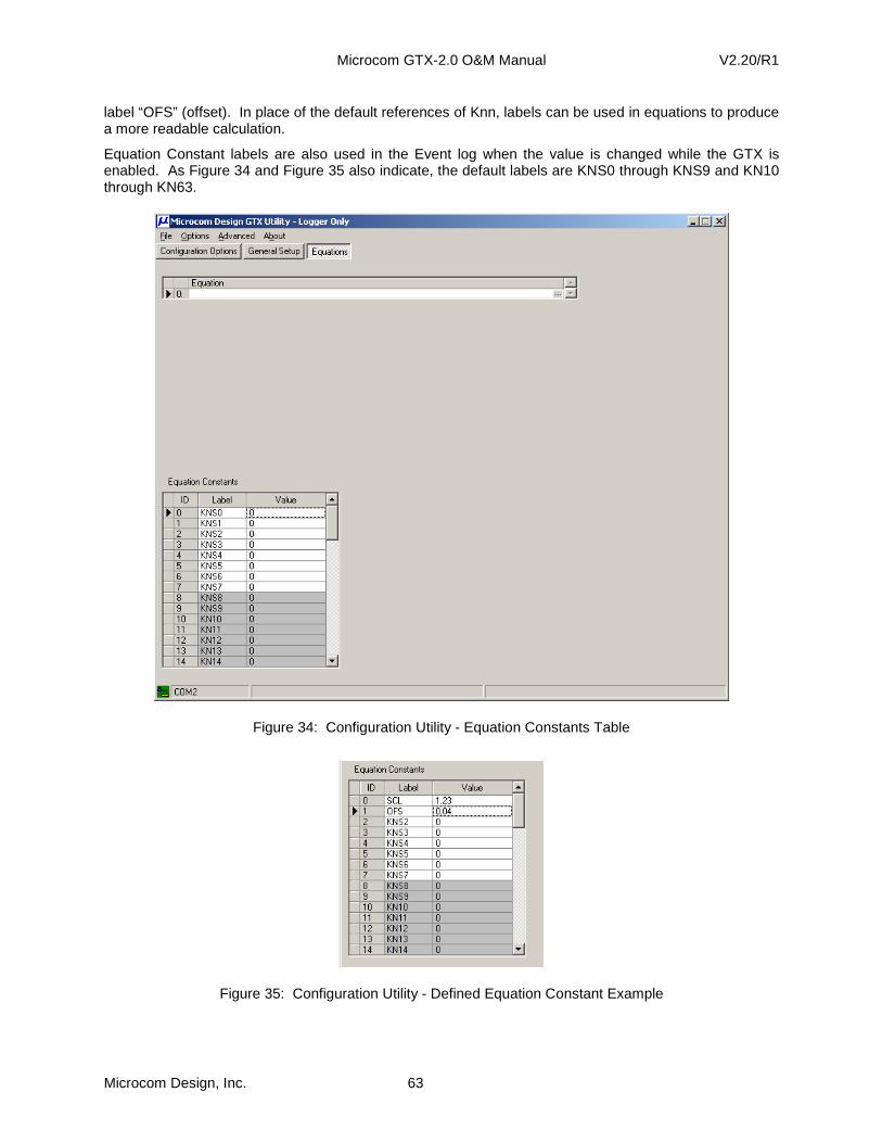
Microcom GTX-2.0 O&M Manual V2.20/R1
Microcom Design, Inc. 63
label “OFS” (offset). In place of the default references of Knn, labels can be used in equations to produce a more readable calculation.
Equation Constant labels are also used in the Event log when the value is changed while the GTX is enabled. As Figure 34 and Figure 35 also indicate, the default labels are KNS0 through KNS9 and KN10 through KN63.
Figure 34: Configuration Utility - Equation Constants Table
Figure 35: Configuration Utility - Defined Equation Constant Example
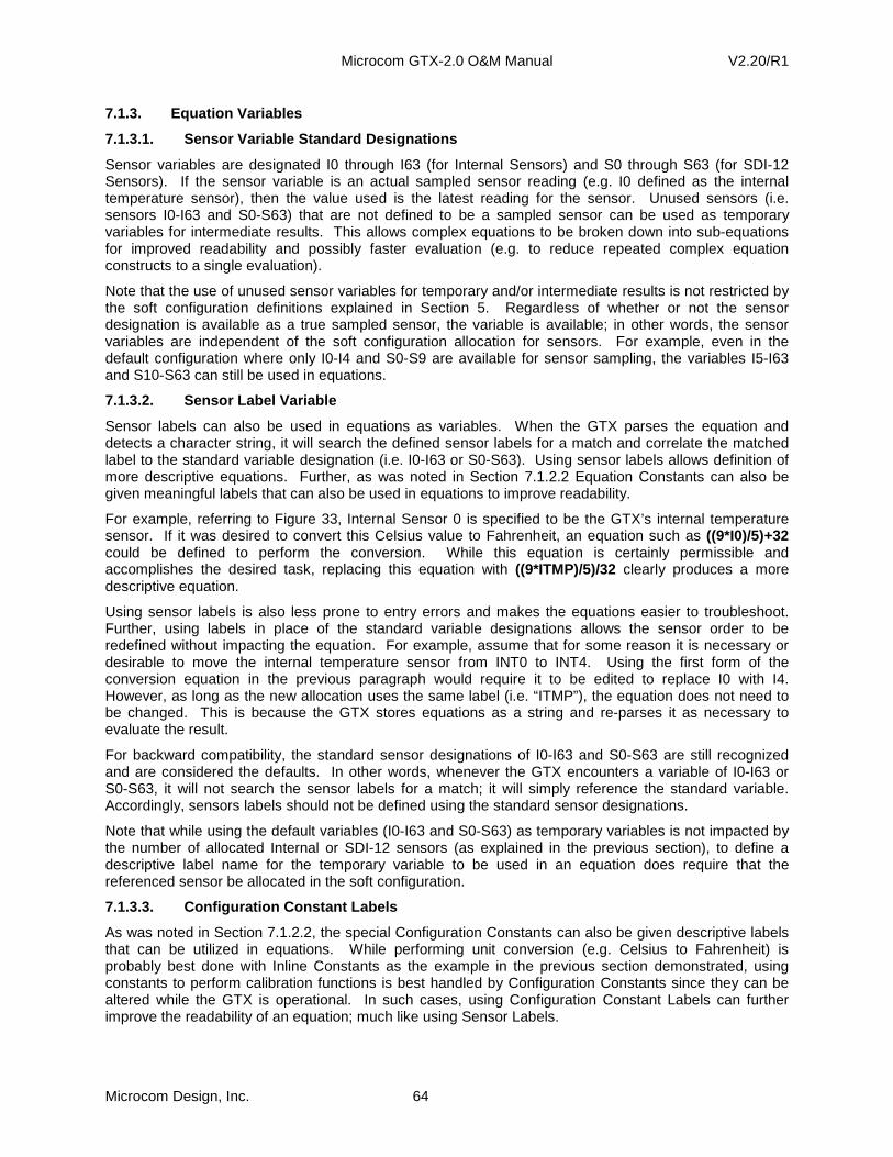
Microcom GTX-2.0 O&M Manual V2.20/R1
Microcom Design, Inc. 64
7.1.3. Equation Variables
7.1.3.1. Sensor Variable Standard Designations
Sensor variables are designated I0 through I63 (for Internal Sensors) and S0 through S63 (for SDI-12 Sensors). If the sensor variable is an actual sampled sensor reading (e.g. I0 defined as the internal temperature sensor), then the value used is the latest reading for the sensor. Unused sensors (i.e. sensors I0-I63 and S0-S63) that are not defined to be a sampled sensor can be used as temporary variables for intermediate results. This allows complex equations to be broken down into sub-equations for improved readability and possibly faster evaluation (e.g. to reduce repeated complex equation constructs to a single evaluation).
Note that the use of unused sensor variables for temporary and/or intermediate results is not restricted by the soft configuration definitions explained in Section 5. Regardless of whether or not the sensor designation is available as a true sampled sensor, the variable is available; in other words, the sensor variables are independent of the soft configuration allocation for sensors. For example, even in the default configuration where only I0-I4 and S0-S9 are available for sensor sampling, the variables I5-I63 and S10-S63 can still be used in equations.
7.1.3.2. Sensor Label Variable
Sensor labels can also be used in equations as variables. When the GTX parses the equation and detects a character string, it will search the defined sensor labels for a match and correlate the matched label to the standard variable designation (i.e. I0-I63 or S0-S63). Using sensor labels allows definition of more descriptive equations. Further, as was noted in Section 7.1.2.2 Equation Constants can also be given meaningful labels that can also be used in equations to improve readability.
For example, referring to Figure 33, Internal Sensor 0 is specified to be the GTX’s internal temperature sensor. If it was desired to convert this Celsius value to Fahrenheit, an equation such as ((9*I0)/5)+32 could be defined to perform the conversion. While this equation is certainly permissible and accomplishes the desired task, replacing this equation with ((9*ITMP)/5)/32 clearly produces a more descriptive equation.
Using sensor labels is also less prone to entry errors and makes the equations easier to troubleshoot. Further, using labels in place of the standard variable designations allows the sensor order to be redefined without impacting the equation. For example, assume that for some reason it is necessary or desirable to move the internal temperature sensor from INT0 to INT4. Using the first form of the conversion equation in the previous paragraph would require it to be edited to replace I0 with I4. However, as long as the new allocation uses the same label (i.e. “ITMP”), the equation does not need to be changed. This is because the GTX stores equations as a string and re-parses it as necessary to evaluate the result.
For backward compatibility, the standard sensor designations of I0-I63 and S0-S63 are still recognized and are considered the defaults. In other words, whenever the GTX encounters a variable of I0-I63 or S0-S63, it will not search the sensor labels for a match; it will simply reference the standard variable. Accordingly, sensors labels should not be defined using the standard sensor designations.
Note that while using the default variables (I0-I63 and S0-S63) as temporary variables is not impacted by the number of allocated Internal or SDI-12 sensors (as explained in the previous section), to define a descriptive label name for the temporary variable to be used in an equation does require that the referenced sensor be allocated in the soft configuration.
7.1.3.3. Configuration Constant Labels
As was noted in Section 7.1.2.2, the special Configuration Constants can also be given descriptive labels that can be utilized in equations. While performing unit conversion (e.g. Celsius to Fahrenheit) is probably best done with Inline Constants as the example in the previous section demonstrated, using constants to perform calibration functions is best handled by Configuration Constants since they can be altered while the GTX is operational. In such cases, using Configuration Constant Labels can further improve the readability of an equation; much like using Sensor Labels.

Microcom GTX-2.0 O&M Manual V2.20/R1
Microcom Design, Inc. 65
For example, assume SDI-12 sensor S0 is tied to some form of a water level sensor that requires a first order field calibration; i.e. slope and offset. Further, assume that this SDI-12 sensor is given the label “WLVL” and that’s its desired to use Configuration Constants K0 and K1 to perform the linear calibration. An Internal Sensor can be tied to an equation of the form K0*WLVL+K1 to perform the correction.
While this is certainly permissible, the two Configuration Constants can be labeled as the example in Section 7.1.2.2 with the descriptive names “SCL” and “OFS”. If this is done, then the equation can be defined as SCL*WLVL+OFS. While this equation performs the calculation, it better defines the intended functionality.
It should be emphasized that the standard constant designations can be used interchangeably with constant labels. As such, whenever the GTX encounters K0-K63 in an equation, it will not search the labels for a match; it will simply utilize the appropriate standard Configuration Constant designation. Accordingly, constant labels should not be defined using the standard constant designations (nor the standard sensor labels for that matter).
7.1.3.4. MMA Processor Variables
As explained in Section 8, the GTX provides a convenient mechanism to facilitate the capture and computation of the minimum, maximum and average for a sensor reading or equation result. The resultant output(s) of the MMA processors can also be used as variables in equations. The GTX provides two mechanisms to reference these outputs; standard variable designators and pseudo functions, which will be covered in the next two sections.
When setting up an MMA Processor, the user ties the processor to a specific sensor reading or equation output, and defines the MMA processing interval. As values are collected, they are automatically forwarded to the MMA Processor and acted upon in real-time. At the end of the user defined processing interval, the final min, max and/or average can be logged and/or stored in a transmission buffer.
While the final MMA interval results are automatically processed for logging and buffer storage, they are retrieved for use in an equation when the equation executes. Therefore, to ensure the equation processes the full interval minimum, maximum and/or average, equations that use these values should be configured to execute shortly after the MMA interval is complete and before the next sample is collected.
For example, assume an average hourly temperature is being computed by an MMA processor with the temperature sensor being read every fifteen minutes. If the samples are collected at 0, 15, 30 and 45 minutes into the hour, then the MMA processor should be set up with a one hour interval and an offset just after the final sample is collected at 45 minute mark and accounting for the sampling time of the sensor, e.g. 00:45:05 . Likewise, any equation that depends on this hourly average should also have a one hour interval with an execution offset that causes the equation to also be evaluated just after the final sensor reading is collected, but before the next sample time occurs.
However, it is not necessary to provide any additional time delay to ensure the MMA Processor completes it processing before the equation executes. This is because the values extracted from the MMA Processor are not the last updated min, max or average, but are instead a live value computed as requested by the equation processor. Further, the min, max and average intermediate processing values are not cleared or reset at the end of the MMA interval. Instead, the intermediate values remain intact and a flag is set to direct them to be reset or cleared once the next sample is collected.
This implementation allows equations that utilize MMA results as variables to be executed at any time after the last sample is collected and before the first sample is collected in the new interval. Further, since the MMA values used in equations are live calculated values, the first time an equation executes the values from the MMA Processor will be valid even if collection process began part way into the interval.
7.1.3.4.1. MMA Variables Standard Designations
Similar to the standard designations for Internal Sensors, SDI-12 Sensors, and Configuration Constants the standard designations for MMA variable consist of a single letter followed by a numeric value from 0 to 63. The standard letter designators are ‘N’, ‘X’, ‘G’, and ‘C’ representing minimum, maximum,
Microcom GTX-2.0 O&M Manual V2.20/R1
Microcom Design, Inc. 66
average, and count; respectively. The count variable is simply the number of samples that have been collected to determine the min, max and average.
While the sensor standard designators (I0-I63 and S0-S63) can be used in equations regardless of whether or not the sensor is defined, the same is not true for the MMA variables (i.e. N0-N63, X0-X63, G0-G63, and C0-C63). In order for a MMA variable to be used in an equation, the corresponding MMA Processor must be defined.
When validating an entered equation, the GTX will declare an error if the equation references an undefined MMA Processor variable. Further, if an MMA Processor is undefined subsequent to the equation validation, the MMA variable value used when the equation executes will always be NaN (Not-a-Number), and the final result of the equation will also be NaN.
Unlike sensor variables, the output of an equation cannot be assigned to an MMA variable.
7.1.3.4.2. MMA Variables Pseudo Functions
While the standard MMA variable designators provide a simple approach to referencing them in equations, their use is somewhat cryptic. Accordingly, the GTX firmware supports four pseudo function references to access these values. The four pseudo functions are: MIN(var), MAX(var), AVG(var), and CNT(var).
These are referred to as pseudo functions since they are entered into an equation using a function format; function name with an argument enclosed in parentheses. However, unlike an arithmetic function (see next section), the argument can only be a single sensor variable reference.
The variable reference for the argument can be either a standard sensor variable designator (e.g. I0 or S0), or it can be a sensor label. In other words, when the equation processor detects the MMA pseudo function name, it looks for only a standard variable or a sensor label within the parentheses and validates it as a sensor reference tied to an MMA Process.
For example, AVG(I0) is equivalent to G0 and CNT(S2) is equivalent to C2. If the label for I0 is defined as “ITMP” as in the various examples in this manual, then following are all equivalent …
G0 ⇔ AVG(I0) ⇔ AVG(ITMP) C0 ⇔ CNT(I0) ⇔ CNT(ITMP) N0 ⇔ MIN(I0) ⇔ MIN(ITMP) X0 ⇔ MAX(I0) ⇔ MAX(ITMP) The use of pseudo functions for MMA variable references improves the readability of the equations with very little penalty in storage requirements, i.e. longer equation require more soft configuration memory.
7.1.4. Equation Arithmetic Functions
The GTX-2.0 equation processor includes a variety of standard and transcendental functions. The available functions are listed in Table 11. Arguments for the functions can be constants, default sensor variables (e.g. I0), sensor labels, or sub-equations (e.g. SQRT(I0*S0)).

Microcom GTX-2.0 O&M Manual V2.20/R1
Microcom Design, Inc. 67
Name Function Format Result ABS Absolute Value ABS(X) absolute value of X CEIL Ceiling CEIL(X) smallest integer > X
FLOOR Floor FLOOR(X) smallest integer < X RND Round RND(X) closest integer to X
SQRT Square Root SQRT(X) square root of X (same as X^0.5) SIN Sine SIN(A) sine of angle, A in degrees COS Cosine COS(A) cosine of angle, A in degrees TAN Tangent TAN(A) tangent of angle, A in degrees ASIN Arcsine ASIN(X) arcsine of X, result in degrees ACOS Arccosine ACOS(X) arccosine of X, result in degrees ATAN Arctangent ATAN(X,Y) arctangent of X & Y, result in degrees LOG Logarithm LOG(X) log base 10 of X LN Natural Log LN(X) log base e of X
EXP Exponential EXP(X) e raised to the X power FMOD Float Modulo FMOD(X,Y) floating point modulus of X relative to Y VALOK Value OK VALOK(X) 1.0 if X is a valid value, 0.0 if not
Table 13: Equation Arithmetic Functions
7.2. Format Specifiers for Equations
As noted Section 7.1.1, the Equation Processor also allows the user to specify the format and precision of the end result of an equation. Two format specifiers are provided, “nF” and “nG”. Preceding each of these format specifiers is a numeric value (n) between 0 and 7 defining the precision or significant digits of the result.
The “nF” format specifier directs the GTX to format the result with a fixed number of digits after the decimal point. For example, a format specifier of 3F will produce a result with the format “±x … x.xxx” ; i.e. the number of digits to the left of the decimal point depends on the value, but the number of digits to right is always fixed at 3. If the magnitude of the value is less than 1.0, then a single 0 will follow the sign character (as in the SDI-12 format, a sign character, + or -, is always included); e.g. for a format of 3F with a magnitude of less than 1, the result will be “±0.xxx”.
The “nG” format specifier directs the GTX to format the result with maximum number of significant digits; i.e. the sum of the significant digits before and after the decimal point will always less than or equal “n”. For example, a format specifier of “3G” for a value of 1.234 will produce a result in the format “+1.23”; a value of 12.34 with the “3G” will yield “+12.3”. Where necessary, place holder digits (0’s) will be included, but do not add into the significant digit count. However, the “nG” format attempts to produce a result with the fewest number of characters; e.g. if the result is 1.23 and the format specify is “5G”, then the result will be in the format of “+1.23” since appending 0’s does not affect the number of significant digits and makes the string result longer. The “nG” format will also utilize the standard exponent format (“±x.xxxEnn”) if it results in fewer characters. For example, a value of 123,000,000 with a format specifier of “3G” will yield “+1.23E+08” since this is more compact than “+123000000”.
To specify the format for the equation result, the equation must be terminated with “@nF” or “@nG”. For example, the equation “S0+S1@3F” will sum S0 and S1 and produce a result with 3 decimal places. If the format specify is omitted, then the default specifier of “7G” will be used, ensuing the result is processed with the maximum number of significant digits possible for the IEEE 4-byte floating-point format.
Note that the equation capability and format specifiers provide a simple mechanism to re-format sampled data. For example, assume a SDI-12 sensor S0 provides a measurement with 5 decimal places, but it is desired to only produce logged results with 3 decimal places, defining an equation “S0@3F”, and operating on the equation result instead of the raw sample will yield logged values with the desired precision.
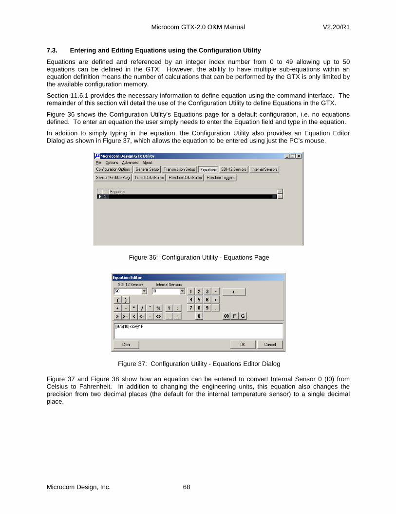
Microcom GTX-2.0 O&M Manual V2.20/R1
Microcom Design, Inc. 68
7.3. Entering and Editing Equations using the Confi guration Utility
Equations are defined and referenced by an integer index number from 0 to 49 allowing up to 50 equations can be defined in the GTX. However, the ability to have multiple sub-equations within an equation definition means the number of calculations that can be performed by the GTX is only limited by the available configuration memory.
Section 11.6.1 provides the necessary information to define equation using the command interface. The remainder of this section will detail the use of the Configuration Utility to define Equations in the GTX.
Figure 36 shows the Configuration Utility’s Equations page for a default configuration, i.e. no equations defined. To enter an equation the user simply needs to enter the Equation field and type in the equation.
In addition to simply typing in the equation, the Configuration Utility also provides an Equation Editor Dialog as shown in Figure 37, which allows the equation to be entered using just the PC’s mouse.
Figure 36: Configuration Utility - Equations Page
Figure 37: Configuration Utility - Equations Editor Dialog
Figure 37 and Figure 38 show how an equation can be entered to convert Internal Sensor 0 (I0) from Celsius to Fahrenheit. In addition to changing the engineering units, this equation also changes the precision from two decimal places (the default for the internal temperature sensor) to a single decimal place.

Microcom GTX-2.0 O&M Manual V2.20/R1
Microcom Design, Inc. 69
Figure 38: Configuration Utility - Equations - Temperature Conversion
Figure 39 shows how the equation can be tied to Internal Sensor 4 and how the internal temperature sensor can now be logged in Fahrenheit instead of Celsius.
Figure 39: Configuration Utility - Equations - Logging Temperature in ºF
Figure 40 shows how the equation can be modified to use the sensor label from Internal Sensor 0 (“ITMP”) to make the equation more descriptive. As noted in Section 7.1.3.2, using the sensor label does not affect the processing of the equation, it simply makes the equation more readable, i.e. the equations in Figure 38 and Figure 40 are identical from the standpoint of the equation processing and end result.
Figure 40: Configuration Utility - Equations - Temperature Conversion with Label
By using the Equations page and assigning additional equations to Internal Sensors substantial processing and evaluation of sampled data can be readily accomplished.
7.4. If-Construct (?) for Equations
An If-Construct can be defined by using the ? (question mark) operator. If-Constructs allow the user to execute one or more sub-equations based on the result of the “if” test. The general format for an If-Construct is shown below.
Microcom GTX-2.0 O&M Manual V2.20/R1
Microcom Design, Inc. 70
<asgn> = <cond>? <true> : <false>;
where, <asgn> is an assignment variable (e.g. I0) <cond> is the condition to test <true> is the equation(s) to execute if <cond> is true (i.e. not equal to zero) <false> is the equation(s) to execute if <cond> is false (i.e. equal to zero)
As shown above, the condition (<cond>) to test is terminated with a question mark (‘?’), and the <true> and <false> equations are separated by a colon (‘:’). The <false> equations must be terminated with a semi-colon if additional equations not part of the If-Construct are to be executed; the semi-colon can be omitted or replaced with the format specifier (‘@’), when the If-Construct is the last equation.
Within the <true> or <false> portions of the If-Construct, multiple sub-equations can be executed. However, these sub-equations must be separated by commas only (i.e. semi-colons can not be used).
As with all equations, the result of the If-Construct is the last sub-equation evaluated. However, with an If-Construct, this is the last sub-equation evaluated within the <true> or <false> list depending on the result of the condition. Likewise, this result can be optionally assigned to a specified variable.
If-Constructs can be used to return a simple variable. For example, “I0=(S0>I0)? S0 : I0;” will set I0 to the maximum of S0 and I0.
If-Constructs can also be used to effectively create subroutines. For example, the equation below can be used to set I3 equal to the average of the last ten samples of I0. In this example, I1 is used to count the number of I0 samples (i.e. I1=I1+1), and I2 is used to accumulate the I0 samples (i.e. I2=I0+I2). Once ten samples have been accumulated (I1=10), the final intermediate sum is calculated (I3=I0+I2), the count and sum values are cleared (I1=0 and I2=0), and the average is computed (I3/10).
I1=I1+1; I3=(I1=10)? I3=I0+I2, I1=0, I2=0, I3/10 : I2=I0+I2, I3;
Note that in the example above, the result of the If-Construct is explicitly assigned to I3. However, the value assigned to I3 is NOT the result of the conditional portion (I1=10) of the construct as might first appear. Instead, the value assigned to I3 is the result of the last equation executed in either the <true> (I3/10) or the <false> (I3) portion of the If-Construct. The inclusion of I3 at the end of the <false> portion ensures that I3 is always equal to the last average computed and does not get assigned to the intermediate sums (i.e. I2=I0+I2).
As noted previously, format specifiers can also be utilized with If-Constructs. For example, defining the equation “(S5>S6)? S5 : S6@2F” and tying it to an Internal Sensor, not only sets the Internal Sensor to the maximum of S5 or S6, it also formats the value to two decimal places, regardless of whether the <true> clause is executed (i.e. S5) or the <false> clause executed (i.e. S6). In other words, the format specifier applies to the If-Construct, not just the <false> portion.
It is not possible to directly nest If-Constructs; for example, attempting to define the equation below will return the error message “ERR: Nested If Test”.
I1=(I0=0)? 0 : (I0>0)? +1 : -1;
However, by using temporary values and multiple consecutive If-Constructs, the same effect the desired can be achieved. For example, the equation below will result in I1 being set to zero if I0=0, I1 being set to +1 if I0>0, or I1 being set to -1 if I0<0. Note that following the first test, I1 will either equal zero or will equal I0; if I1 is set to zero, than the following to tests will both fail and in both cases I1 will be set equal to itself. However, if I0 is not zero, then I1 will be set to I0 after the first test and one of the following decisions must yield a true result.
I1=(I0=0)? 0 : I0; I1=(I1>0)? +1 : I1; I1=(I1<0)? -1 : I1
The “if” condition does not necessarily have to yield a value of 1.0 to be “true” (as occurs when using the relational operators), any non-zero value is also considered “true”. Conversely, only a result of zero (0.0) yields a “false” result. As such, the “if” test (I0<>0)? is equivalent to simply (I0)?
Microcom GTX-2.0 O&M Manual V2.20/R1
Microcom Design, Inc. 71
Finally, it should be noted that the If-Construct operator (‘?’) has higher precedence than the assignment operator, but lower precedence then any mathematical functions. This means the equation “I0=I0+1>10?” increments I0 by 1, tests the intermediate result (I0+1) to see if it is greater than 10, and assigns the appropriate result of the <true> or <false> clause to I0. To increment I0 by 1, save the incremented value to I0, and then perform the test; the equation must be broken into two parts, i.e. “I0=I0+1; I0>10?”. While parenthesis around the “if” condition are not absolutely necessary, they do help to clarify the intent and actual execution of If-Construct.
7.5. Equation Initial Conditions
Once the GTX is enabled and the clock is set, equations will be processed on the time schedule defined by their associated Internal Sensor configuration. Since the time at which equation processing begins is typically not at any specific time, it is important to understand the initial conditions and variable settings to understand how equations are handled to avoid erroneous results until valid sensor readings are available.
7.5.1. Initial Sensor, Variable, and Equation Value s
By default, all unused sensor/variables (I0-I63 and S0-S63) are initialized to zero when the GTX is enabled. However, any defined Internal or SDI-12 sensors are preset to a special value that is designated as NaN (not-a-number). If an equation is executed before a valid sensor reading is acquired to replace this special value, then the result of that equation will also be NaN. In general, executing any equation with one or more input variables equal to NaN produces an NaN result.
If the resulting value from an equation is NaN and the Internal Sensor that is tied to this equation is referenced in a transmission buffer, then no value is copied to the transmission buffer. In other words, the transmission buffer value remains null and is filled in with slashes or spaces based on the setting of the Slash Fill flag (see Section 9.7). This protection mechanism ensures that erroneous, albeit possibly realistic, values are not inadvertently transmitted. For example, assume an equation is defined to convert a temperature reading from Celsius to Fahrenheit and that the temperature sensor has not been sampled before the equation executes. If the initial value for the corresponding temperature value was initialized to zero, then the result of the equation would 32 (°F). While this may be a realistic value, it is m ost likely not the correct reading for the current temperature.
If it is desirable for a particular sensor variable to have an explicitly defined initial value, then this can be accomplished using an Initialization Equation as will be detailed in the next section.
7.5.2. Initialization Equations
While equations are primarily intended to be tied to an Internal Sensor so that the equations will be executed on a scheduled basis, equations do not necessarily have to be tied to an Internal Sensor. Any equation that is not tied to an Internal Sensor is considered an Initialization Equation. Initialization Equations are executed whenever the GTX is enabled for operation. Since these equations are executed only once (when the unit is placed in the enabled state), they provide a convenient mechanism to explicitly initialize variables.
Using an Initialization Equation, any variable can be explicitly initialized to any value (e.g. I0=10). This feature can be useful to initially set a counter variable to a value other than zero. It can also be used to initialize a variable to a default value to produce a valid output the first time it is executed.
As another example, assume an equation is defined to capture a maximum value of a sensor. If the sensor readings can never be negative (e.g. wind speed), then allowing the maximum variable to default to zero does not present a problem as the new reading is guaranteed to be equal to or greater than 0. However, for sensor readings that can have valid negative values (e.g. temperature), an initial value of zero will not ensure the maximum is properly captured; as long as the value is negative, the default initial value of zero will be considered the maximum reading. To avoid this, an Initialization Equation can be utilized to default the variable to a sufficiently negative value (e.g. -100) to ensure the first reading is always captured as the maximum.

Microcom GTX-2.0 O&M Manual V2.20/R1
Microcom Design, Inc. 72
It should also be noted, that the Min, Max, and Average Processor described in Section 8, eliminates the need to initialize variables to capture minimums and maximums since it provides the requisite processing to ensure the first captured sensor value is always set as the initial minimum and maximum.
Note that when a variable is explicitly initialized, this initialization only sets the internal value of the variable; it does not constitute a sensor reading (i.e. the initial values are not logged nor are they forwarded to the transmission buffers). In other words, the initial value simply sets the starting value that will be used in subsequent equations when they are first executed.
7.6. Default Labels, Standard Designators, Function s
As was discussed in the preceding sections, the GTX Equation Processor can utilize Labels and Standard Designators to represent Sensor, Configuration Constants, and MMA values. For Sensors (Internal and SDI-12) and Configuration Constants, the GTX also provides “Default Labels”. While the user can naturally change the Labels from there defaults, the Default Labels can also be utilized “as is”.
However, Default Labels are not the same as the Standard Designators. When a string matching a Standard Designator is found in an Equation, the GTX never performs a Label or Function lookup; it simply uses the designator to access the corresponding value or uses it to determine the appropriate Pseudo-Function of the MMA Processor.
On the other hand, if the Equation Processor encounters a string that does not match a Standard Designation, then it tries to match it to a function reference or label. If the user hasn’t provided a custom Label for a Sensor or Constant, the GTX assumes the Default Label in the search algorithm.
Table 14 summarizes the Standard Designators, and the corresponding Default Labels or MMA Pseudo Functions used by the GTX-2.0. When defining Labels, the user should avoid using any of the Standard Designators. Failure to do so can produce unexpected results as the GTX will recognize the designators before searching the labels. The user should also avoid using MMA Pseudo-Function or Arithmetic Function (Table 13) names as Labels as well.
Parameter
Standard Designators
Default Label or Pseudo Function
Internal Sensor I0-I63 INT0-INT9 and IN10-IN63 SDI-12 Sensor S0-S63 SDI0-SDI9 and SD10-SD63
Configuration Constant K0-K63 KNS0-KNS9 and KN10-KN63 MMA Minimum N0-N63 MIN() MMA Maximum X0-X63 MAX() MMA Average G0-G63 AVG() MMA Count C0-C63 CNT()
Table 14: Standard Designators and Default Label Summary
Two other important distinction between Standard Designators, Functions, and Labels, and Functions that need to be made are how the GTX handles letter case and the order in which the GTX looks for these tokens. The search order and case rules is summarized below:
• Standard Designators: Are case sensitive; e.g. “I0” is recognized as Standard Designator, but “i0” is not.
• Functions: Are case insensitive; e.g. LN() and ln() are both recognized as the Natural Logarithm function. This applies to both Arithmetic and MMA Pseudo Functions.
• Labels: Are case sensitive; e.g. INT0 is not the same as int0. Labels can also mix case; e.g. TEMP, Temp, and temp are all valid, but are not interchangeable.
Since Functions are recognized before Labels and Functions are case insensitive, Labels should not be defined as a mixed or lower case version any function reference; if the Equation Processor is to be used. Naturally, if the user’s application does not require calculations, then the Equation Processor will not be required and this caution is not applicable.

Microcom GTX-2.0 O&M Manual V2.20/R1
Microcom Design, Inc. 73
8. Min, Max, Average (MMA) Processor
The Microcom GTX-2.0 also implements a special equation processor to allow the user to easily generate cumulative information for a sensor or equation result. The Min, Max, and Average Processor (MMA) allows the user to define a process to accumulate, log and transmit the minimum and maximum value sampled over a given interval, along with being able to easily calculate the average value of the samples over the interval.
Up to 64 MMA Processes can be defined in the GTX. For each process, the user must specify the sensor (Internal or SDI-12) to accumulate MMA data. Since Internal Sensors can also be tied to equations, an MMA Process can therefore operate on the result of an equation as well as sampled sensor data. Further, the min, max, and average results can then be used in subsequent equations as explained in Section 7.1.3.3.
8.1. MMA Basics and Configuration Utility Definitio n
When defining an MMA Process, the sensor to be accumulated must be specified along the accumulation interval (or rate). An optional accumulation offset allows the user to specify exactly when the Min, Max, and Average data will be collected and processed within the interval. Finally, the user can specify which, if any, MMA results are logged to the Data/Event buffer.
Figure 41: Configuration Utility - Sensor Min Max Avg Page
Section 11.6.6 details the use of the command interface to setup MMA Processes. The remainder of this section will detail the setup steps using the Configuration Utility. Note that once an MMA Process is

Microcom GTX-2.0 O&M Manual V2.20/R1
Microcom Design, Inc. 74
defined, the resultant data can also be included in a transmission buffer as explained in Section 9.4.3 (configuration utility), and Section 11.7.3 (command line interface).
Figure 41 shows the main MMA page of the Configuration Utility. This page consists of a single grid with 8 columns and 64 rows. The rows are numbered 0 through 63 corresponding to the index number of the MMA Processor. It also shows the page with all MMA Processors disabled, i.e. set to “None”. To define an MMA Processor, simply click on the drop-down arrow in the desired MMA Processor and select the desired sensor as shown in Figure 42.
Figure 42: Configuration Utility - Defining an MMA Processor
Once the desired sensor is selected, the user can fill in the remaining columns. The Interval column specifies the processing interval for the MMA Processor, i.e. how often the Min, Max, and Average values will be collected and processed. The Offset column specifies exactly when in the Interval, the processing will occur. It useful to ensure the last data value in the Interval has been forwarded to the MMA Processor. The default Offset is 00:00:00.
For MMA Processes, Intervals must be in the range of 00:00:10 to 24:00:00 (i.e. ten seconds to once a day). Offsets can be 00:00:00 (i.e. no offset), and any value less than the Interval. For Intervals and Offsets less than 12:00:00, the value can be defined to the second. However, Intervals and Offsets between 12:00:00 and 24:00:00 must have an even second; i.e. the resolution is 2 seconds.
The “Min”, “Max”, and “Avg” columns provide checkboxes (once the sensor has been defined). Checking the appropriate box instructs the GTX to log the equivalent parameter in the Data/Event Log.

Microcom GTX-2.0 O&M Manual V2.20/R1
Microcom Design, Inc. 75
This process is can be repeated for as many MMA Processor as the application requires. Note that the use of the Configuration Utility frees the user from having to specify the maximum number of MMA Processors to allocate in the soft configuration memory using the MMN command (see Sections 5 and 11.6.4). The Configuration Utility will set the maximum number to provide sufficient processors as specified by the “Sensor Min Max Avg” page.
Figure 43: Configuration Utility - Configuring an MMA Processor
Figure 43 shows a completed MMA Processor for Internal Sensor “ITMP”. If “ITMP” is configured as shown in Figure 33, then it will be sampled every 15 minutes, and the minimum, maximum, and average values will be logged on a daily basis. Note that the Offset for this MMA Processor is set to 23:45:10; with this setting the MMA data will be captured and processed 10 seconds after the last value of the day is processed. Referring back to Figure 33, the first sample of each day occurs right at midnight. Whether or not the midnight sample is the first sample of the new day or the last sample is at the users discretion, and either case can be easily accommodated by adjusting the Offset setting.
8.2. MMA Vector Average
A special case of the MMA processor that can be defined is to perform a vector average. Vector averaging is useful when trying to average a directional value, such as degrees. When averaging degrees, an erroneous result will most likely occur when individual values fluctuate around the 0° and 360° transition point. For example, the correct av erage of 1° and 359° should be 0°, but the numerica l average of these two values is 180.

Microcom GTX-2.0 O&M Manual V2.20/R1
Microcom Design, Inc. 76
Checking, the “Vec” box for a MMA directs the GTX to perform a unity gain vector average. In this mode of operation, the values are assumed to be in degrees and the sine and cosine values are computed then summed. When the average is computed the summed values are converted back to degrees using a four quadrant arctangent function.
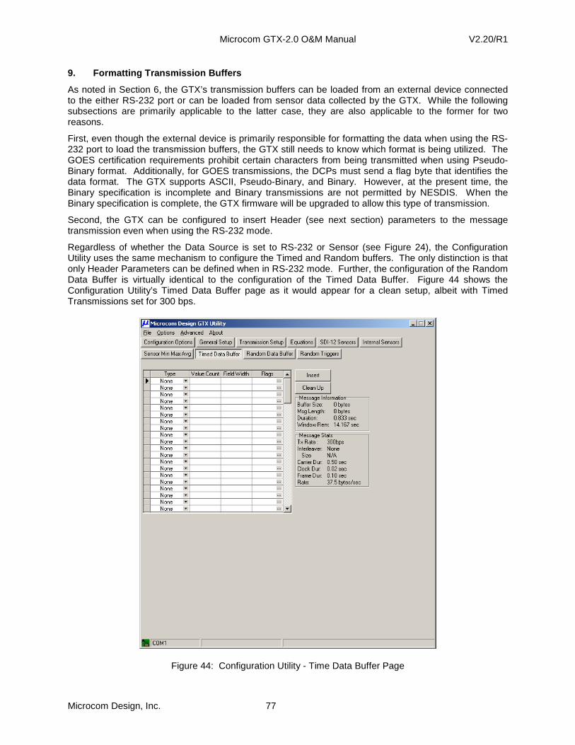
Microcom GTX-2.0 O&M Manual V2.20/R1
Microcom Design, Inc. 77
9. Formatting Transmission Buffers
As noted in Section 6, the GTX’s transmission buffers can be loaded from an external device connected to the either RS-232 port or can be loaded from sensor data collected by the GTX. While the following subsections are primarily applicable to the latter case, they are also applicable to the former for two reasons.
First, even though the external device is primarily responsible for formatting the data when using the RS-232 port to load the transmission buffers, the GTX still needs to know which format is being utilized. The GOES certification requirements prohibit certain characters from being transmitted when using Pseudo-Binary format. Additionally, for GOES transmissions, the DCPs must send a flag byte that identifies the data format. The GTX supports ASCII, Pseudo-Binary, and Binary. However, at the present time, the Binary specification is incomplete and Binary transmissions are not permitted by NESDIS. When the Binary specification is complete, the GTX firmware will be upgraded to allow this type of transmission.
Second, the GTX can be configured to insert Header (see next section) parameters to the message transmission even when using the RS-232 mode.
Regardless of whether the Data Source is set to RS-232 or Sensor (see Figure 24), the Configuration Utility uses the same mechanism to configure the Timed and Random buffers. The only distinction is that only Header Parameters can be defined when in RS-232 mode. Further, the configuration of the Random Data Buffer is virtually identical to the configuration of the Timed Data Buffer. Figure 44 shows the Configuration Utility’s Timed Data Buffer page as it would appear for a clean setup, albeit with Timed Transmissions set for 300 bps.
Figure 44: Configuration Utility - Time Data Buffer Page
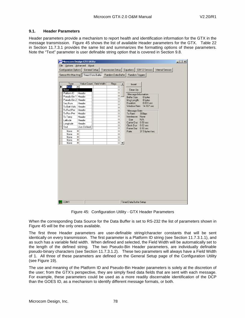
Microcom GTX-2.0 O&M Manual V2.20/R1
Microcom Design, Inc. 78
9.1. Header Parameters
Header parameters provide a mechanism to report health and identification information for the GTX in the message transmission. Figure 45 shows the list of available Header parameters for the GTX. Table 22 in Section 11.7.3.1 provides the same list and summarizes the formatting options of these parameters. Note the “Text” parameter is user definable string option that is covered in Section 9.8.
Figure 45: Configuration Utility - GTX Header Parameters
When the corresponding Data Source for the Data Buffer is set to RS-232 the list of parameters shown in Figure 45 will be the only ones available.
The first three Header parameters are user-definable string/character constants that will be sent identically on every transmission. The first parameter is a Platform ID string (see Section 11.7.3.1.1), and as such has a variable field width. When defined and selected, the Field Width will be automatically set to the length of the defined string. The two Pseudo-Bin Header parameters, are individually definable pseudo-binary characters (see Section 11.7.3.1.2). These two parameters will always have a Field Width of 1. All three of these parameters are defined on the General Setup page of the Configuration Utility (see Figure 19).
The use and meaning of the Platform ID and Pseudo-Bin Header parameters is solely at the discretion of the user; from the GTX’s perspective, they are simply fixed data fields that are sent with each message. For example, these parameters could be used as a more readily discernable identification of the DCP than the GOES ID, as a mechanism to identify different message formats, or both.
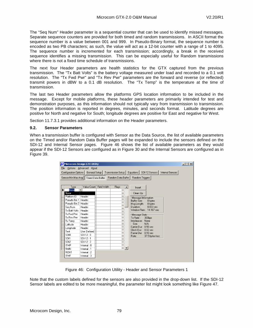
Microcom GTX-2.0 O&M Manual V2.20/R1
Microcom Design, Inc. 79
The “Seq Num” Header parameter is a sequential counter that can be used to identify missed messages. Separate sequence counters are provided for both timed and random transmissions. In ASCII format the sequence number is a value between 001 and 999. In Pseudo-Binary format, the sequence number is encoded as two PB characters; as such, the value will act as a 12-bit counter with a range of 1 to 4095. The sequence number is incremented for each transmission; accordingly, a break in the received sequence identifies a missing transmission. This can be especially useful for Random transmissions where there is not a fixed time schedule of transmissions.
The next four Header parameters are health statistics for the GTX captured from the previous transmission. The “Tx Batt Volts” is the battery voltage measured under load and recorded to a 0.1 volt resolution. The “Tx Fwd Pwr” and “Tx Rev Pwr” parameters are the forward and reverse (or reflected) transmit powers in dBW to a 0.1 dB resolution. The “Tx Temp” is the temperature at the time of transmission.
The last two Header parameters allow the platforms GPS location information to be included in the message. Except for mobile platforms, these header parameters are primarily intended for test and demonstration purposes, as this information should not typically vary from transmission to transmission. The position information is reported in degrees, minutes, and seconds format. Latitude degrees are positive for North and negative for South; longitude degrees are positive for East and negative for West.
Section 11.7.3.1 provides additional information on the Header parameters.
9.2. Sensor Parameters
When a transmission buffer is configured with Sensor as the Data Source, the list of available parameters on the Timed and/or Random Data Buffer pages will be expanded to include the sensors defined on the SDI-12 and Internal Sensor pages. Figure 46 shows the list of available parameters as they would appear if the SDI-12 Sensors are configured as in Figure 30 and the Internal Sensors are configured as in Figure 39.
Figure 46: Configuration Utility - Header and Sensor Parameters 1
Note that the custom labels defined for the sensors are also provided in the drop-down list. If the SDI-12 Sensor labels are edited to be more meaningful, the parameter list might look something like Figure 47.

Microcom GTX-2.0 O&M Manual V2.20/R1
Microcom Design, Inc. 80
Figure 47: Configuration Utility - Header and Sensor Parameters 2
The list of available Sensor parameters is continuously, and dynamically adjusted, as the user edits the SDI-12 and Internal Sensor pages. The drop-down list of Header and Sensor parameters greatly simplifies the setup of the transmission buffers as will be shown in Sections 9.4.1 and 9.4.2.
9.3. ASCII Versus Pseudo-Binary Formatting
Before detailing the process of setting up a Data Buffer, a brief description of the two types of formats, ASCII versus Pseudo-Binary, will be instructive.
When a DCP is configured for ASCII messages, data is sent using the ASCII character set and sensor readings are typically formatted as numeric values in engineering units. ASCII messages quite often label the measurements and utilize various white space characters and delimiters (e.g. spaces, commas, carriage returns, etc.). While this approach provides a message structure that can be easily read upon receipt, it also can significantly increases the message size and duration; even to the point where the message length may exceed the allotted time window.
While the GTX supports the ASCII format for platforms that require it, it also supports Pseudo-Binary messages. Pseudo-Binary formatting can greatly reduce the message size, which allows more data points to be sent than would be possible using ASCII formatted data. Pseudo-binary format is generally preferred by the GOES DCS user community, and is strongly recommended by NOAA/NESDIS.
Pseudo-Binary format is an encoding scheme that utilizes a subset of the ASCII character set. Each byte transmitted is an ASCII character and contains 6 bits of binary information. The pseudo-binary character set is provided in the table below.
As shown in Table 15, the 64 characters from @ to DEL represent a contiguous range of values from 0 to 63. With the exception of DEL, the characters are all ASCII printable. While it is permissible to transmit the DEL character, the Pseudo-binary specification allows the ? character to be used in place of the DEL so that all the characters are printable.

Microcom GTX-2.0 O&M Manual V2.20/R1
Microcom Design, Inc. 81
Char Hex Value Char Hex Value Char Hex Value Char Hex Value @ 40 0 P 50 16 ‘ 60 32 p 70 48 A 41 1 Q 51 17 a 61 33 q 71 49 B 42 2 R 52 18 b 62 34 r 72 50 C 43 3 S 53 19 c 63 35 s 73 51 D 44 4 T 54 20 d 64 36 t 74 52 E 45 5 U 55 21 e 65 37 u 75 53 F 46 6 V 56 22 f 66 38 v 76 54 G 47 7 W 57 23 g 67 39 w 77 55 H 48 8 X 58 24 h 68 40 x 78 56 I 49 9 Y 59 25 i 69 41 y 79 57 J 4A 10 Z 5A 26 j 6A 42 z 7A 58 K 4B 11 [ 5B 27 k 6B 43 { 7B 59 L 4C 12 \ 5C 28 l 6C 44 | 7C 60 M 4D 13 ] 5D 29 m 6D 45 } 7D 61 N 4E 14 ^ 5E 30 n 6E 46 ~ 7E 62 O 4F 15 _ 5F 31 o 6F 47 DEL 7F 63 ? 3F 63
Table 15: Pseudo-Binary Character Set
Using a single pseudo-binary character allows one of 64 values to be represented. To represent more values, multiple characters are used. Specifically, two characters can be used to represent a 12-bit value, which yields a range of 0 to 4095 or 4096 distinct values (64*64=4096). If necessary, three and fours characters can be used to represent 18 and 24 bit values, respectively.
The key to using pseudo-binary is range limiting and scaling. For example, the GTX uses a single pseudo-binary character to represent the battery voltage under load. Since it can be reasonably assumed that the battery voltage under load will be in the range of 9.0 to 15.3 VDC, the GTX converts the battery reading to an integer in the range of 0 to 63 by subtracting 9 and multiplying by 10. The resulting integer is then encoded using the table above. For battery reading of 12.5 the result is 35 = 10*(12.5-9.0), in which case the GTX would load and transmit the ‘c’ character for this reading.
As the battery voltage example shows, range limiting is accomplished by adding or subtracting an offset and scaling is applied to convert the value to an integer to the desired precision. The scale value is also known as the “slope”. By choosing the appropriate slope and offset values most readings can be readily converted to one or two pseudo-binary characters. Note that by converting the battery voltage to pseudo-binary format, the number of characters required to represent the reading is reduced from a maximum of four (e.g. 12.5) to just one character (e.g. ‘c’).
Values that can be both positive and negative can be handled in one of two ways: 1) an offset can be added to shift the range of numbers to all positive values, or 2) the data can be converted to a two’s-complement value. Two’s-complement representation is a method of expressing negative numbers so subtraction may be performed by a simple fixed-precision binary accumulator (adder). The negative value is computed by complementing each bit and then adding 1. For example the value 5 is represented in 6-bits as 000101, while the value of –5 is represented as 111011 (111010+000001). Note that most computers represent negative integers in two’s-complement format. An alternative method of determining the two’s-complement representation is to subtract the value from the 2N , where N is the number of bits to be used. For example, 26-5 = 64-5 = 59 = 111011.
A good example of a signed parameter is the internal temperature sensor, which has a resolution of 0.25°C. To represent a temperature range of -40°C to +60°C to ¼°C requires 400 unique values (4*100), which can be easily accomplished with two pseudo-binary characters using a slope of 4 and an offset of 40. The offset value ensures all the readings are positive and is an example of the first approach to handling negative values. However, if an offset value of zero is used the data will have to be represented in two’s-complement format.
Microcom GTX-2.0 O&M Manual V2.20/R1
Microcom Design, Inc. 82
When configuring a pseudo-binary parameter for inclusion in a transmission buffer, the user specifies the pseudo-binary number of characters to use by setting the desired character count in the Field Width column (see Figure 56). A positive Field Width indicates the readings will be unipolar, while a negative Field Width will direct the GTX to use two’s-complement format.
Note that the GTX will clamp any readings outside the permissible range to the appropriate extreme value. For example, for a Field Width of 2, the maximum range for a 12-bit value is 0 to 4095; as such, negative values will be clamped to 0, and values equal to 4096 or greater will be clamped to 4095. For a Field Width of –2, the maximum range for a 12-bit value is –2048 to +2047; values outside this range will be clamped to the closest permissible value.
Returning to the temperature example, using an offset of 40 allows the range of values to be expressed unipolar. For example, a temperature reading of –10.25°C would be represented by the pseudo-binary character string ‘Aw’. Table 15 can be used to convert this representation back to engineering units; note that since the first pseudo-binary character represents the upper 6-bits of the 12-bit value, the equivalent value of this character from Table 15 must be multiplied by 64. Specifically, the string ‘Aw’ is equivalent to (1*64)+55 = 129 (i.e. A=1 and w=55). Applying the inverse scaling and offset yields (119/4)-40 = -10.25.
For a 0 offset with a Field Width of –2, this same value would be represented as ‘?W’. Converting this value back to engineering units is performed using a similar procedure with one extra step. First, the ‘?W’ is converted to a positive integer using Table 15; specifically, (63*64)+23 = 4055 (i.e. ?=63 and W=23). Now this value must be subtracted from 212=4096 and inverse scaled; i.e. (4055-4096)/4 = -41/4 = -10.25.
Note that in both cases, converting the temperature readings from ASCII to pseudo-binary reduces the required number of characters from six (e.g. –10.25) to two (e.g. ‘Aw’ or ‘?W’). The two simple examples used in this section, battery voltage and temperature, demonstrate the power of pseudo-binary formatting. Specifically, it provides the ability to reduce message sizes by as much as 67% to 75%. The next two sections, which provide detailed examples of ASCII and pseudo-binary formatting, will expand on this ability to compress message lengths using the pseudo-binary approach.
9.3.1. Rounding versus Truncating for Transmission Buffers
In addition to affecting the message length and transmission time, use of ASCII versus Pseudo-Binary format also determines whether data values are truncated or rounded when stored in a transmission buffer. However, before detailing the truncation and rounding procedures applied by the GTX, it is important to note that when data values are passed to the transmission buffers they are always passed as an ASCII string. In the case of SDI-12 parameters, the string value is directly captured from the SDI-12 sensor. For Internal Sensors the ASCII string is in the default format for the specific sensor (e.g. temperature, tipping bucket, etc.) or in the format specified as part of the equation (see Section 7.2).
When using ASCII for a transmission buffer, the string value is simply copied to the appropriate location in the buffer. As explained in Section 9.4.1, the user specifies the field width for each ASCII value. As such, the field width should be sufficiently specified to allow the entire string to fit. If the field width is less than the string length, then characters are dropped from the right. Accordingly, any decimal places that won’t fit are simply truncated; i.e. the value is not rounded.
However, using equations and format specifiers (see Section 7.2), rounding a value to any specified precision can be easily accomplished. For example, if an SDI-12 sensor reports it’s value to 3 decimal places but the user wishes to transmit the value with only 1 decimal place, an equation that simply references this value with the format specifier “@1F” can be used. The format specifier not only reduces the number of decimal places in the resultant ASCII string, it also performs a rounding operation.
When using Pseudo-Binary for the transmission, all values are converted from their ASCII string format to a floating-point value, appropriately offset and scaled, rounded to a whole number, and then converted to pseudo-binary. As such, there is an inherent rounding operation in the conversion process. In other words, conversion to pseudo-binary always rounds values before storing them in the transmission buffer.
It should be emphasized that rounding and/or truncation operations described above only apply when storing values in a transmission buffer. When values are stored in the Data/Event log, they are always stored to the maximum precision possible; i.e. based on the number significant digits in the value up to a

Microcom GTX-2.0 O&M Manual V2.20/R1
Microcom Design, Inc. 83
maximum of 7 (the maximum precision of a standard IEEE 4-byte floating point value). Further, as explained in Sections 7 and 8, respectively, the Equation and MMA Processors always use the values converted to a IEEE 4-byte floating point value. As such, these processes also do not round values below the maximum of 7 significant digits.
9.4. Data Buffer Configuration
The following two subsections will provide examples of how to utilize the Configuration Utility to complete the definitions of the Timed and Random Data Buffers. For the purpose of these examples, it is assumed that the GTX is to be configured as shown in Figure 48 and Figure 49.
Figure 48: Configuration Utility - Data Buffer - Internal Sensor Setup
Specifically, the internal sensors will provide a temperature reading, an accumulated rain value (scaled tipping bucket value to 0.01”), and the raw tipping bucket counts. Further, only one SDI-12 sensor is utilized that provides a water level reading in feet to a hundredth of a foot (i.e. 0.01’). All sensor readings will be collected on a 15 minute schedule, and it is assumed the GTX will be transmitting on an hourly schedule.
Figure 49: Configuration Utility - Data Buffer - SDI-12 Sensor Setup
9.4.1. Timed Data Buffer Configuration Example – AS CII Formatting
While the preferred method of message formatting is pseudo-binary (per NOAA/NESDIS), this section will provide an example of configuring the GTX’s Timed Data Buffer for ASCII transmissions. The following section provides a similar example on how to configure the Random Data Buffer for pseudo-binary transmissions.
To configure the timed message structure, the user utilizes the Timed Data Buffer page to select the desired parameters to be included in the buffer as shown in Figure 47.

Microcom GTX-2.0 O&M Manual V2.20/R1
Microcom Design, Inc. 84
Figure 50 shows the Timed Data Buffer configuration with the first three parameters defined as Header parameters “Tx Batt Volts”, “Tx Fwd Pwr”, and “Tx Rev Pwr”. Note that when Header parameters are defined, the Configuration Utility automatically fills in the Value Count and Field Width columns and “greys” them out indicating that these values cannot be altered. The Value Count determines the number of historical readings that are to be included and the Field Width determines the number of characters to reserve in the message stream. Header parameters will always have a Value Count of 1, and the Field Width is determined by the GTX.
As shown in Figure 50, the three Header parameters selected all have Field Width of 5 characters. Accordingly, at this point the “Message Information” box reports a “Buffer Size” of 15 bytes; the message length (“Msg Length) for a HDR transmission is always 8 bytes more as the total message size includes the 4-byte GOES ID, the HDR flag byte, an EOT character, and two flush bytes (4+1+1+2 = 8) per the NESDIS HDR Certification. The Message Information also provides information on the actual length of the message, i.e. the “Duration” in seconds, and also the amount of time remaining in the defined transmission window.
Figure 50: Configuration Utility - Timed Data Buffer Header Configuration 1
9.4.1.1. Timed Data Buffer Configuration Example – ASCII Flags
The “Flags” column is used to define additional formatting options for the associated record or parameter. Clicking the “…” button in the cell launches the “Record Format Flags” dialog as shown in Figure 51. This dialog allows the user to specify a “Label” to precede the value and can be used to select various “Record Terminators”, i.e. “Space”, “Carriage Return”, and/or “Line Feed”.

Microcom GTX-2.0 O&M Manual V2.20/R1
Microcom Design, Inc. 85
Figure 51: Configuration Utility - Record Format Flags Dialog
9.4.1.1.1. Timed Data Buffer Configuration Example – Labels
Labels and Record Terminators are fixed strings and white-space characters that can improve the readability of an ASCII message. While the use of these feature is strongly discouraged for operational platforms as they increase the message duration, they can be quite useful for test and demonstration purposes.
Figure 52: Configuration Utility - Timed Data Buffer Header Configuration 2
Enabling the “Label” option for a field also enables the radio group to define whether or not a colon should be included with the label text, and if so, its location. The default mode is to include the colon after the label (e.g. “RAIN:”). However, the user also has the option to have the colon precede the label (e.g. “:RAIN”) or omit the colon completely. See Section 11.7.3 for information on how to specify the label options using the terminal commands.
9.4.1.1.2. Timed Data Buffer Configuration Example – Record Terminators
Each transmit record can be optionally terminated with a Space, a Carriage Return (CR), and/or a Line Feed (LF) as shown in Figure 51. When multiple terminators are specified, they are included in a prioritized order of space then CR then LF. For example, selecting Carriage Return and Line Feed always results in the CR being output before the LF.
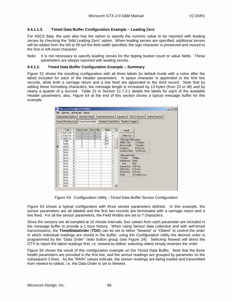
Microcom GTX-2.0 O&M Manual V2.20/R1
Microcom Design, Inc. 86
9.4.1.1.3. Timed Data Buffer Configuration Example – Leading Zero
For ASCII data, the user also has the option to specify the numeric value to be reported with leading zeroes by checking the “Add Leading Zero” option. When leading zeroes are specified, additional zeroes will be added from the left to fill out the field width specified; the sign character is preserved and moved to the first or left-most character.
Note: It is not necessary to specify leading zeroes for the tipping bucket count or value fields. These parameters are always reported with leading zeroes.
9.4.1.2. Timed Data Buffer Configuration Example – Summary
Figure 52 shows the resulting configuration with all three labels (in default mode with a colon after the label) included for each of the Header parameters. A space character is appended to the first two records, while both a carriage return and a line feed are appended to the third record. Note that by adding these formatting characters, the message length is increased by 13 bytes (from 23 to 36) and by nearly a quarter of a second. Table 22 in Section 11.7.3.1 details the labels for each of the available Header parameters; also, Figure 54 at the end of this section shows a typical message buffer for this example.
Figure 53: Configuration Utility - Timed Data Buffer Sensor Configuration
Figure 53 shows a typical configuration with three sensor parameters defined. In this example, the sensor parameters are all labeled and the first two records are terminated with a carriage return and a line feed. For all the sensor parameters, the Field Widths are set to 7 characters.
Since the sensors are all sampled at 15 minute intervals, four values from each parameter are included in the message buffer to provide a 1 hour history. When using Sensor data collection and with self-timed transmissions, the TimedDataOrder (TDO) can be set to either “Newest” or “Oldest” to control the order in which individual readings are stored in the buffer; using the Configuration Utility the desired order is programmed by the “Data Order” radio button group (see Figure 24). Selecting Newest will direct the GTX to report the latest readings first, i.e. newest-to-oldest; selecting oldest simply reverses the order.
Figure 54 shows the result of this configuration example on the Timed Data Buffer. Note that the three health parameters are provided in the first line, and the sensor readings are grouped by parameter on the subsequent 3 lines. As the “RAIN” values indicate, the sensor readings are being loaded and transmitted from newest-to-oldest, i.e. the Data Order is set to Newest.

Microcom GTX-2.0 O&M Manual V2.20/R1
Microcom Design, Inc. 87
As noted previously, the formatting options provide an easily reading message; each parameter is labeled, records are organized in lines, and the sensor readings are in a row-column matrix. Again, while the use of these formatting options can be useful for test and demonstration, it also significantly increases the message duration.
As shown in Figure 53, the total duration for this message format is 4.407 seconds. If just the labeling options are removed, a 16% reduction (3.687 versus 4.407 seconds) in message length can be realized.
Figure 54: Configuration Utility - Timed Data Buffer Example
Section 11.7.1 provides the necessary information to use the terminal commands to setup the Timed Data Buffer. Provided below is the list of commands to reproduce the configuration shown in the above example.
TDP=0,H4,LS TDP=1,H5,LS TDP=2,H6,LRN TDP=3,I0,4,7,LRN TDP=4,I1,4,7,LRN TDP=5,S0,4,7,L
9.4.2. Random Data Buffer Configuration Example – P seudo-Binary Formatting
In this section, an example of how the Configuration Utility can be used to configure the Random Data Buffer will be provided. This example will use a similar configuration to the example in the previous
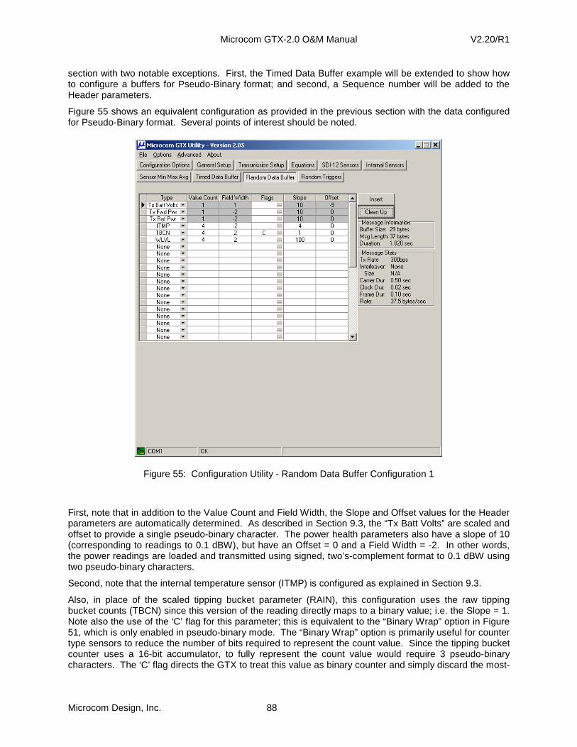
Microcom GTX-2.0 O&M Manual V2.20/R1
Microcom Design, Inc. 88
section with two notable exceptions. First, the Timed Data Buffer example will be extended to show how to configure a buffers for Pseudo-Binary format; and second, a Sequence number will be added to the Header parameters.
Figure 55 shows an equivalent configuration as provided in the previous section with the data configured for Pseudo-Binary format. Several points of interest should be noted.
Figure 55: Configuration Utility - Random Data Buffer Configuration 1
First, note that in addition to the Value Count and Field Width, the Slope and Offset values for the Header parameters are automatically determined. As described in Section 9.3, the “Tx Batt Volts” are scaled and offset to provide a single pseudo-binary character. The power health parameters also have a slope of 10 (corresponding to readings to 0.1 dBW), but have an Offset = 0 and a Field Width = -2. In other words, the power readings are loaded and transmitted using signed, two’s-complement format to 0.1 dBW using two pseudo-binary characters.
Second, note that the internal temperature sensor (ITMP) is configured as explained in Section 9.3.
Also, in place of the scaled tipping bucket parameter (RAIN), this configuration uses the raw tipping bucket counts (TBCN) since this version of the reading directly maps to a binary value; i.e. the Slope = 1. Note also the use of the ‘C’ flag for this parameter; this is equivalent to the “Binary Wrap” option in Figure 51, which is only enabled in pseudo-binary mode. The “Binary Wrap” option is primarily useful for counter type sensors to reduce the number of bits required to represent the count value. Since the tipping bucket counter uses a 16-bit accumulator, to fully represent the count value would require 3 pseudo-binary characters. The ‘C’ flag directs the GTX to treat this value as binary counter and simply discard the most-

Microcom GTX-2.0 O&M Manual V2.20/R1
Microcom Design, Inc. 89
significant bits (i.e. it disables the clamping of values as discussed in Section 9.3). In this example, this operation effectively reduces the tipping bucket counter from 16 to 12 bits, reducing the number of pseudo-binary characters needed by 1. Note that this same operation can also be accomplished by setting the Tipping Bucket Rollover Count to 4096 (see Sections 6.1.2.1.2.2 and 11.5.3.11).
Figure 56: Configuration Utility - Random Data Buffer Configuration 2
Next, the water level parameter utilizes a Slope of 100 and an Offset of 0 with a Field Width of 2. This scaling allows the data to be represented to the maximum resolution of 0.01’ with a range of 0.00’ to 40.95’. Since the Filed Width is positive it is assumed the actual values cannot be negative.
By utilizing pseudo-binary format and removing all formatting characters (labels and record terminators), the message duration is reduced from 4.407 seconds to 1.820 seconds, or nearly 41%.
As a final step in this example, Figure 56 shows the result of inserting the “Seq Num” Header parameter and adding record terminators to the fourth through sixth parameters. Adding a sequence number to a random report can aid in identifying missed messages, which can result on Random channels due to DCP message collisions.
Adding the record terminators is done simply to facilitate the comparison of the Timed Data Buffer and Random Data Buffer values in the examples from Figure 54 and Figure 57. In other words, since the data values shown in these figures are from the same set of collection samples, the last three lines can be directly compared to demonstrate the ASCII to pseudo-binary conversion.
For example, the first tipping bucket count (TBCN) from Figure 57 is ‘@L’, which correlates to (0*64)+12 = 12, which is equivalent to 000.12” of “RAIN” from Figure 54. The remaining readings can likewise be compared.
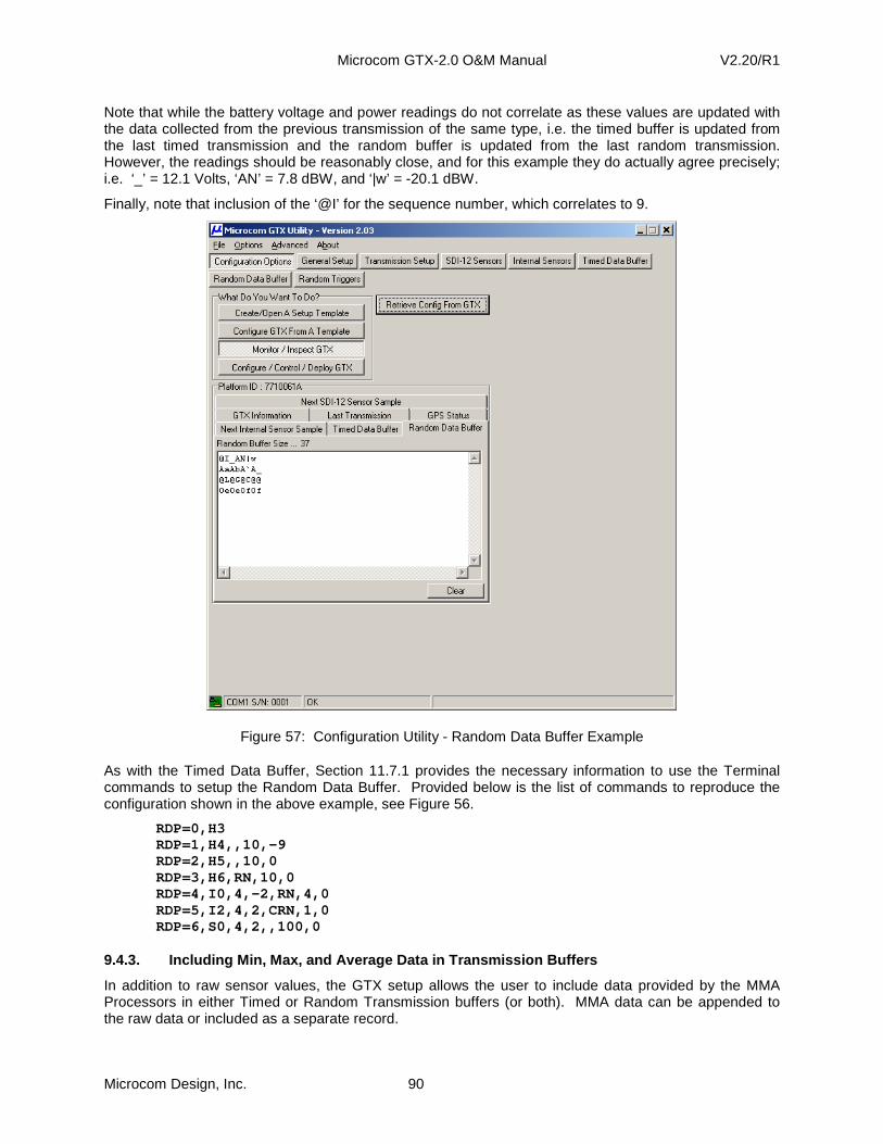
Microcom GTX-2.0 O&M Manual V2.20/R1
Microcom Design, Inc. 90
Note that while the battery voltage and power readings do not correlate as these values are updated with the data collected from the previous transmission of the same type, i.e. the timed buffer is updated from the last timed transmission and the random buffer is updated from the last random transmission. However, the readings should be reasonably close, and for this example they do actually agree precisely; i.e. ‘_’ = 12.1 Volts, ‘AN’ = 7.8 dBW, and ‘|w’ = -20.1 dBW.
Finally, note that inclusion of the ‘@I’ for the sequence number, which correlates to 9.
Figure 57: Configuration Utility - Random Data Buffer Example
As with the Timed Data Buffer, Section 11.7.1 provides the necessary information to use the Terminal commands to setup the Random Data Buffer. Provided below is the list of commands to reproduce the configuration shown in the above example, see Figure 56.
RDP=0,H3 RDP=1,H4,,10,-9 RDP=2,H5,,10,0 RDP=3,H6,RN,10,0 RDP=4,I0,4,-2,RN,4,0 RDP=5,I2,4,2,CRN,1,0 RDP=6,S0,4,2,,100,0
9.4.3. Including Min, Max, and Average Data in Tran smission Buffers
In addition to raw sensor values, the GTX setup allows the user to include data provided by the MMA Processors in either Timed or Random Transmission buffers (or both). MMA data can be appended to the raw data or included as a separate record.

Microcom GTX-2.0 O&M Manual V2.20/R1
Microcom Design, Inc. 91
To append the MMA data, the MMA flags ‘N’, ‘X’, and ‘G’ (corresponding to the last letters in the abbreviations min, max, and avg) are simply appended to the Value Count field as shown in Figure 58. Using this approach simply appends the MMA fields to the sampled data record. These values will always appear after the raw values and in Min, Max, and Average order. Note that the same field width is used for these readings and the effective Value Count is increased by 1 for each MMA parameter selected. As shown in Figure 58, the message length increased by 21 bytes (7 characters for each of the MMA parameters).
Figure 58: Configuration Utility - Appending MMA Data To Transmission Data
To include the MMA data as a separate record (e.g. so the MMA parameters appear on a separate line), a new transmission record must first be inserted, or appended to the list. To only include the MMA data in this record, set the Value Count to 0 and append the desired MMA flags as shown in Figure 59. Note that this is the only time a zero Value Count is permissible.
Using this approach, the label will be identical to the label used for the raw values, but the MMA data will appear on a separate line due to the use of the “LRN” flags; however, the message length has now increased an additional 8 bytes for the label and the line separator characters (CR/LF). If it is desired to use a different label for the MMA data, the raw values can simply be tied to a separate Internal Sensor, and the MMA Processor tied to this separate Internal Sensor. This yields a “virtual” sensor that is equivalent to the raw sample sensor. However, since it is a unique Internal Sensor, it can have a unique label.
For example, assume equation 0 simply equals “I0” (e.g. EQN,0=I0). Now assume that equation 0 is tied to Internal Sensor 4, “I4”, which is executed at the same sample rate as “I0”. If the MMA Processor that was accumulated data for “I0” is simply edited to accumulate data for “I4”, then no effective changes in the processing of the sampled have been altered. However, since “I4” is a unique sensor, it’s label can be changed to “TMMA” (or another descriptor the user deems appropriate). Now the transmission buffer (and the Data/Event Log) will use the label for “I4” when identifying the MMA data for this sensor.
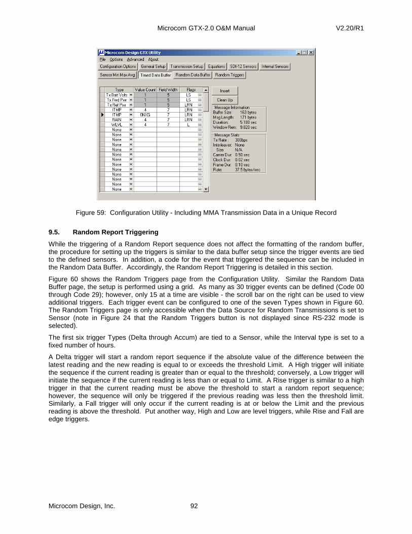
Microcom GTX-2.0 O&M Manual V2.20/R1
Microcom Design, Inc. 92
Figure 59: Configuration Utility - Including MMA Transmission Data in a Unique Record
9.5. Random Report Triggering
While the triggering of a Random Report sequence does not affect the formatting of the random buffer, the procedure for setting up the triggers is similar to the data buffer setup since the trigger events are tied to the defined sensors. In addition, a code for the event that triggered the sequence can be included in the Random Data Buffer. Accordingly, the Random Report Triggering is detailed in this section.
Figure 60 shows the Random Triggers page from the Configuration Utility. Similar the Random Data Buffer page, the setup is performed using a grid. As many as 30 trigger events can be defined (Code 00 through Code 29); however, only 15 at a time are visible - the scroll bar on the right can be used to view additional triggers. Each trigger event can be configured to one of the seven Types shown in Figure 60. The Random Triggers page is only accessible when the Data Source for Random Transmissions is set to Sensor (note in Figure 24 that the Random Triggers button is not displayed since RS-232 mode is selected).
The first six trigger Types (Delta through Accum) are tied to a Sensor, while the Interval type is set to a fixed number of hours.
A Delta trigger will start a random report sequence if the absolute value of the difference between the latest reading and the new reading is equal to or exceeds the threshold Limit. A High trigger will initiate the sequence if the current reading is greater than or equal to the threshold; conversely, a Low trigger will initiate the sequence if the current reading is less than or equal to Limit. A Rise trigger is similar to a high trigger in that the current reading must be above the threshold to start a random report sequence; however, the sequence will only be triggered if the previous reading was less then the threshold limit. Similarly, a Fall trigger will only occur if the current reading is at or below the Limit and the previous reading is above the threshold. Put another way, High and Low are level triggers, while Rise and Fall are edge triggers.

Microcom GTX-2.0 O&M Manual V2.20/R1
Microcom Design, Inc. 93
Figure 60: Configuration Utility - Random Triggers Page
An Accumulation (Accum) trigger is similar to a Delta trigger in that the difference between this reading and a previous reading must exceed the programmed limit. However, while the Delta trigger works on two successive samples (i.e. the previous reading is the last reading), the Accumulation trigger works on the value saved the last time this parameter actually triggered a Random Report sequence. This type of trigger is useful for triggering when a predetermined amount of rainfall has occurred regardless of how often the sensor is sampled, i.e. regardless of how hard it is raining.
The Interval trigger is a special trigger that can be used to ensure a Random Report is triggered every so often as a confidence check that the transmitter is still functional. When defining an Interval trigger, no parameter identification is required or permitted, i.e. the Sensor cell will be grayed out (see Figure 62). For an Interval trigger, the Limit value can be set from 1 to 240 hours (fractional values are not permitted). An Interval trigger will only occur if a Random Report has not been triggered by another defined trigger within the last number of Limit hours.
Figure 61 shows the steps required to define a Sensor trigger event. First, the desired sensor is selected from the drop-down list, and then the threshold Limit is entered. In this example, a Random Report sequence will be triggered whenever a tenth inch of rain is accumulated.
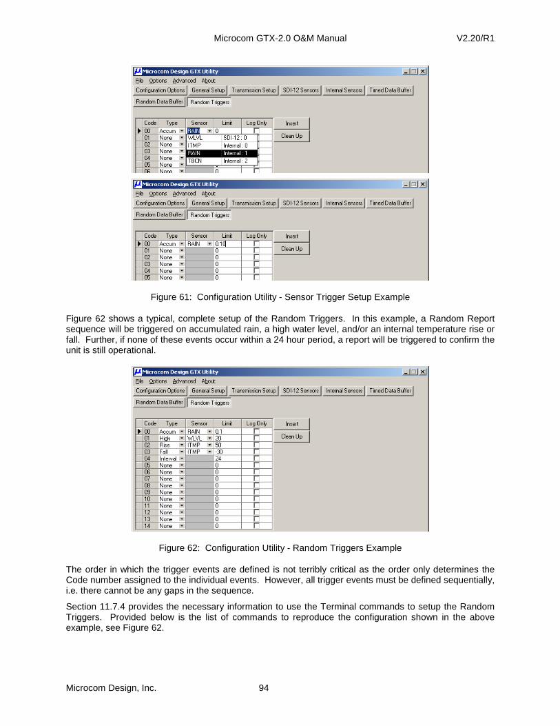
Microcom GTX-2.0 O&M Manual V2.20/R1
Microcom Design, Inc. 94
Figure 61: Configuration Utility - Sensor Trigger Setup Example
Figure 62 shows a typical, complete setup of the Random Triggers. In this example, a Random Report sequence will be triggered on accumulated rain, a high water level, and/or an internal temperature rise or fall. Further, if none of these events occur within a 24 hour period, a report will be triggered to confirm the unit is still operational.
Figure 62: Configuration Utility - Random Triggers Example
The order in which the trigger events are defined is not terribly critical as the order only determines the Code number assigned to the individual events. However, all trigger events must be defined sequentially, i.e. there cannot be any gaps in the sequence.
Section 11.7.4 provides the necessary information to use the Terminal commands to setup the Random Triggers. Provided below is the list of commands to reproduce the configuration shown in the above example, see Figure 62.
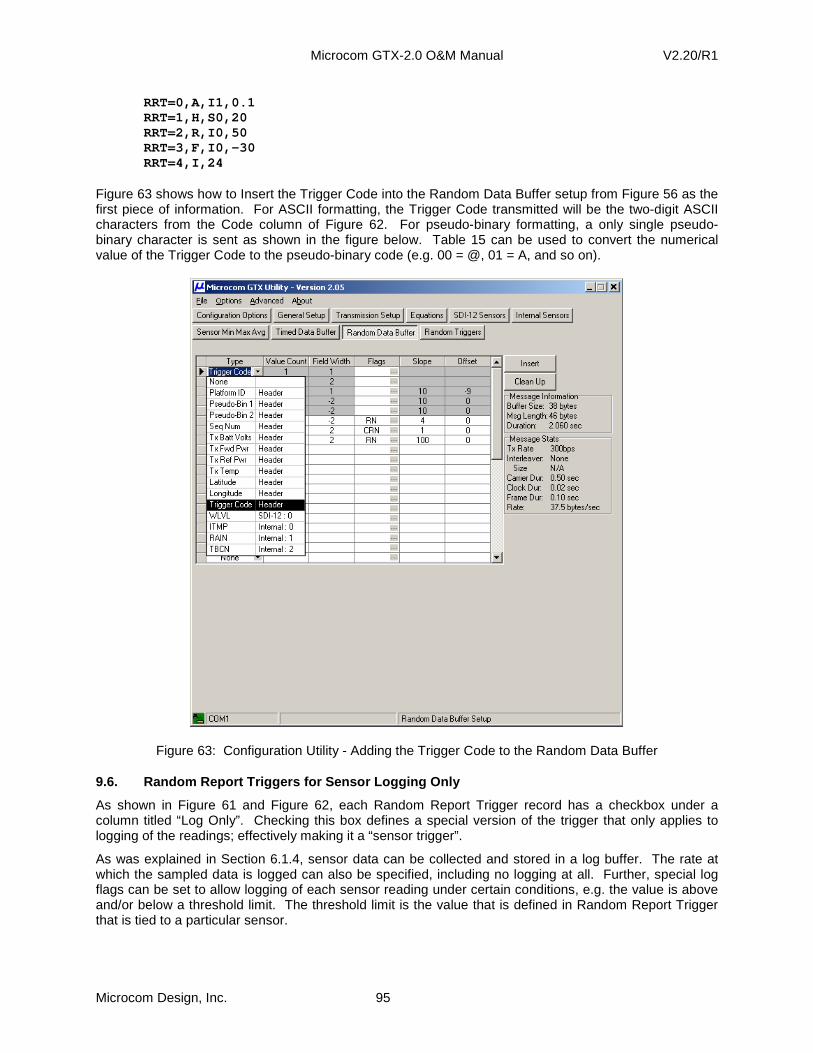
Microcom GTX-2.0 O&M Manual V2.20/R1
Microcom Design, Inc. 95
RRT=0,A,I1,0.1 RRT=1,H,S0,20 RRT=2,R,I0,50 RRT=3,F,I0,-30 RRT=4,I,24
Figure 63 shows how to Insert the Trigger Code into the Random Data Buffer setup from Figure 56 as the first piece of information. For ASCII formatting, the Trigger Code transmitted will be the two-digit ASCII characters from the Code column of Figure 62. For pseudo-binary formatting, a only single pseudo-binary character is sent as shown in the figure below. Table 15 can be used to convert the numerical value of the Trigger Code to the pseudo-binary code (e.g. 00 = @, 01 = A, and so on).
Figure 63: Configuration Utility - Adding the Trigger Code to the Random Data Buffer
9.6. Random Report Triggers for Sensor Logging Only
As shown in Figure 61 and Figure 62, each Random Report Trigger record has a checkbox under a column titled “Log Only”. Checking this box defines a special version of the trigger that only applies to logging of the readings; effectively making it a “sensor trigger”.
As was explained in Section 6.1.4, sensor data can be collected and stored in a log buffer. The rate at which the sampled data is logged can also be specified, including no logging at all. Further, special log flags can be set to allow logging of each sensor reading under certain conditions, e.g. the value is above and/or below a threshold limit. The threshold limit is the value that is defined in Random Report Trigger that is tied to a particular sensor.

Microcom GTX-2.0 O&M Manual V2.20/R1
Microcom Design, Inc. 96
Enabling the “Log Only” option, allows thresholds to be defined for logging purpose without allowing them to trigger a random report. If the example from Figure 62 is modified as shown in Figure 64, then the “RAIN”, “WLVL” and “Interval” triggers will still generate a Random Report sequence when they fire, but the two “ITMP” triggers will not. These two triggers will only be used to affect the logging rate of the “ITMP” readings.
Figure 64: Configuration Utility - “Log Only” Random Triggers Example
9.7. Slash Fill Option for Transmission Buffers
As shown in Figure 19 and detailed in Section 11.3.8, the user can direct the GTX to fill null data fields in a transmission buffer with a forward slash character (‘/’) in place of the default fill process.
In the default case, the GTX initially fills all transmission buffer data fields with space characters. Following the initial fill, the GTX will fill data fields with the appropriate value unless a sensor fails to report its value due to a fault condition.
When the transmission format is ASCII and a sensor fails to provide a value, the GTX will fill the appropriate ASCII field with the string “N/M” (right-justified, sufficient spaces will be added to the left to fill the field) if the field width is greater than three characters. When the field width is three characters or less, the GTX will fill with spaces. When the transmission format is Pseudo-Binary, the GTX defaults to filling with spaces when a sensor fails to respond.
When the Slash Fill option is enabled, the GTX will always fill ASCII and Pseudo-Binary fields with the forward slash character (‘/’). In other words, the transmission buffers will be initially filled with slashes and the appropriate field will be updated with slashes when a sensor fails to respond. One important distinction between ASCII and Pseudo-Binary format is that in Pseudo-Binary format the entire field width is always filled with slashes. However, in ASCII format, a space is loaded into the first character of the field and the remaining characters are filled with slashes when multiple values of the same parameter are to be reported.
The substitution of a space for the first character in a multiple value lists ensures there is at least one white space character between each value which improves readability. Note when only one value is to be reported for a parameter, the entire field is field with slashes.
In addition to identifying null data, the slash fill feature is also useful to better see the structure of the transmission buffer before data is actually collected since the space fill characters are not readily distinguishable when all the fields are null.
For example, Figure 65 shows the Timed Data Buffer from the example in Section 9.4.1 with the Slash Fill option enabled prior to any data collection operations or a timed transmission. The slashes clearly indicate the Field Widths and Value Counts for the setup. Since space characters are not visible, the message structure wouldn’t be as readily discernable.
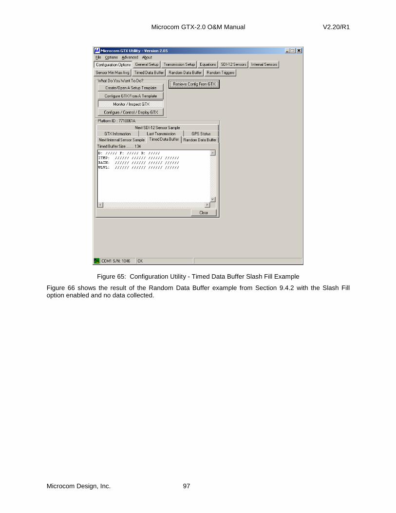
Microcom GTX-2.0 O&M Manual V2.20/R1
Microcom Design, Inc. 97
Figure 65: Configuration Utility - Timed Data Buffer Slash Fill Example
Figure 66 shows the result of the Random Data Buffer example from Section 9.4.2 with the Slash Fill option enabled and no data collected.

Microcom GTX-2.0 O&M Manual V2.20/R1
Microcom Design, Inc. 98
Figure 66: Configuration Utility - Random Data Buffer Slash Fill Example
9.8. Text Transmit Parameter
Text parameters allow fixed text strings to be included in a transmit buffer. While sending fixed text strings in a transmission is not a recommended practice since it increases the size and duration of a message without providing measurement data, legacy GOES transmissions quite often utilized such strings and it may be necessary to include them for backward compatibility.
To enter a fixed text string in a transmission buffer, simply select the Text option in the Type drop down and enter up to a ten character string in the corresponding “Value Count” field as shown in Figure 67.
Figure 67: Configuration Utility - Text Transmit Parameter Example

Microcom GTX-2.0 O&M Manual V2.20/R1
Microcom Design, Inc. 99
Note that when the Text parameter type is selected, the “Field Width” cell is grayed out and not utilized. However, the “Flags” remains in effect allowing the standard terminators of Space, CR, and/or LF to be specified to follow the field.
Text parameters also implement a special case of the labeling option. Specifying the Label option essentially tells the GTX that the text field is to be treated as a “Label”. Accordingly, the GTX will automatically append a colon to the string. The default setting is to place the colon after the text field or label, but placing the colon before the string is also an optional setting (see Figure 51). Figure 68 shows an example of how to use a Text parameter as a label.
Figure 68: Configuration Utility - Text Transmit Parameter as a Label Example
See Section 11.7.3.4 for information on how to specify Text parameters in transmit buffers using Terminal commands.
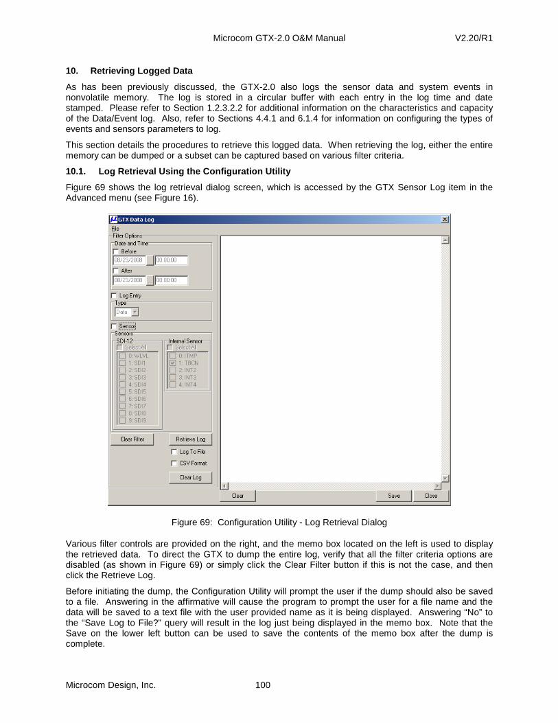
Microcom GTX-2.0 O&M Manual V2.20/R1
Microcom Design, Inc. 100
10. Retrieving Logged Data
As has been previously discussed, the GTX-2.0 also logs the sensor data and system events in nonvolatile memory. The log is stored in a circular buffer with each entry in the log time and date stamped. Please refer to Section 1.2.3.2.2 for additional information on the characteristics and capacity of the Data/Event log. Also, refer to Sections 4.4.1 and 6.1.4 for information on configuring the types of events and sensors parameters to log.
This section details the procedures to retrieve this logged data. When retrieving the log, either the entire memory can be dumped or a subset can be captured based on various filter criteria.
10.1. Log Retrieval Using the Configuration Utility
Figure 69 shows the log retrieval dialog screen, which is accessed by the GTX Sensor Log item in the Advanced menu (see Figure 16).
Figure 69: Configuration Utility - Log Retrieval Dialog
Various filter controls are provided on the right, and the memo box located on the left is used to display the retrieved data. To direct the GTX to dump the entire log, verify that all the filter criteria options are disabled (as shown in Figure 69) or simply click the Clear Filter button if this is not the case, and then click the Retrieve Log.
Before initiating the dump, the Configuration Utility will prompt the user if the dump should also be saved to a file. Answering in the affirmative will cause the program to prompt the user for a file name and the data will be saved to a text file with the user provided name as it is being displayed. Answering “No” to the “Save Log to File?” query will result in the log just being displayed in the memo box. Note that the Save on the lower left button can be used to save the contents of the memo box after the dump is complete.

Microcom GTX-2.0 O&M Manual V2.20/R1
Microcom Design, Inc. 101
The Clear button is used to erase the contents of the memo box, and the Close button will close this dialog.
The Clear Log button is used to erase the entire contents of the Data/Event log. Since the data is irretrievably lost once the memory is cleared, the program will prompt the user to confirm the request to erase the log before proceeding as shown in Figure 70.
Figure 70: Configuration Utility - Log Erasure Comfirmation Dialog
Figure 71 shows an example of a retrieved log. Note that each entry has a 5-digit sequence number and a 3 or 4 character identifier. “STX” and ETX” identify the start and end of a transmission, respectively. The custom sensor labels defined by the user when setting up the sensor collections are used to identify the sensor readings. Following the identifier is the date and time the data was logged, and then the actual data is displayed.
For an “STX” entry, only the type of transmission (TEST, TIMED, or RANDOM) and the start time is logged. The “ETX” entry also includes the type of transmission, but additionally logs the transmission’s battery voltage (in VDC), and forward/reflected power readings (in dBW).
Figure 71: Configuration Utility - Retrieved Log
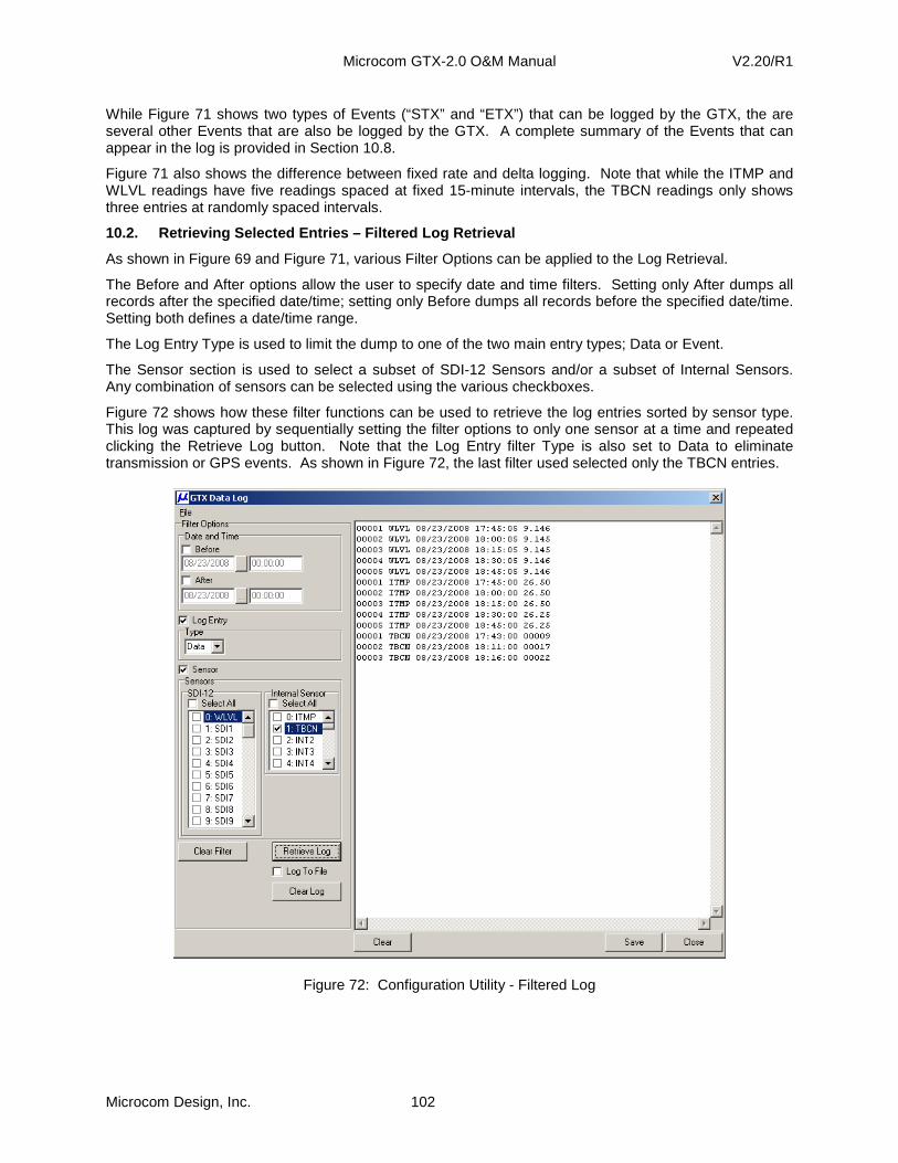
Microcom GTX-2.0 O&M Manual V2.20/R1
Microcom Design, Inc. 102
While Figure 71 shows two types of Events (“STX” and “ETX”) that can be logged by the GTX, the are several other Events that are also be logged by the GTX. A complete summary of the Events that can appear in the log is provided in Section 10.8.
Figure 71 also shows the difference between fixed rate and delta logging. Note that while the ITMP and WLVL readings have five readings spaced at fixed 15-minute intervals, the TBCN readings only shows three entries at randomly spaced intervals.
10.2. Retrieving Selected Entries – Filtered Log Re trieval
As shown in Figure 69 and Figure 71, various Filter Options can be applied to the Log Retrieval.
The Before and After options allow the user to specify date and time filters. Setting only After dumps all records after the specified date/time; setting only Before dumps all records before the specified date/time. Setting both defines a date/time range.
The Log Entry Type is used to limit the dump to one of the two main entry types; Data or Event.
The Sensor section is used to select a subset of SDI-12 Sensors and/or a subset of Internal Sensors. Any combination of sensors can be selected using the various checkboxes.
Figure 72 shows how these filter functions can be used to retrieve the log entries sorted by sensor type. This log was captured by sequentially setting the filter options to only one sensor at a time and repeated clicking the Retrieve Log button. Note that the Log Entry filter Type is also set to Data to eliminate transmission or GPS events. As shown in Figure 72, the last filter used selected only the TBCN entries.
Figure 72: Configuration Utility - Filtered Log
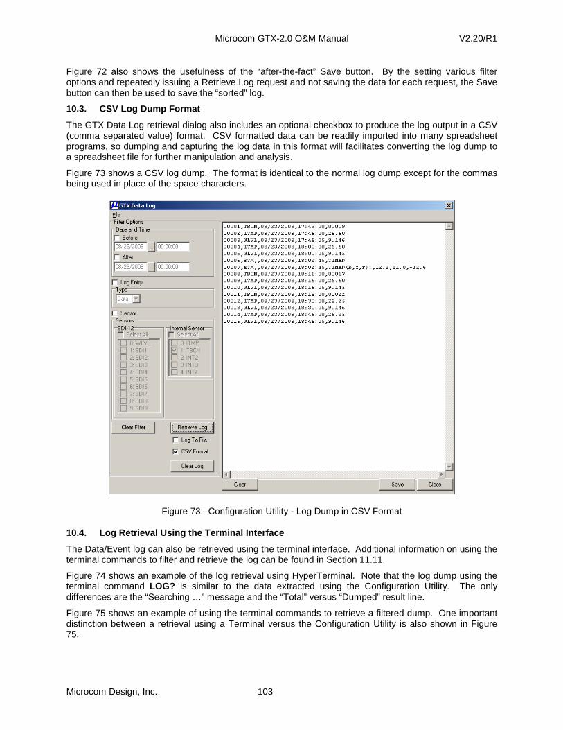
Microcom GTX-2.0 O&M Manual V2.20/R1
Microcom Design, Inc. 103
Figure 72 also shows the usefulness of the “after-the-fact” Save button. By the setting various filter options and repeatedly issuing a Retrieve Log request and not saving the data for each request, the Save button can then be used to save the “sorted” log.
10.3. CSV Log Dump Format
The GTX Data Log retrieval dialog also includes an optional checkbox to produce the log output in a CSV (comma separated value) format. CSV formatted data can be readily imported into many spreadsheet programs, so dumping and capturing the log data in this format will facilitates converting the log dump to a spreadsheet file for further manipulation and analysis.
Figure 73 shows a CSV log dump. The format is identical to the normal log dump except for the commas being used in place of the space characters.
Figure 73: Configuration Utility - Log Dump in CSV Format
10.4. Log Retrieval Using the Terminal Interface
The Data/Event log can also be retrieved using the terminal interface. Additional information on using the terminal commands to filter and retrieve the log can be found in Section 11.11.
Figure 74 shows an example of the log retrieval using HyperTerminal. Note that the log dump using the terminal command LOG? is similar to the data extracted using the Configuration Utility. The only differences are the “Searching …” message and the “Total” versus “Dumped” result line.
Figure 75 shows an example of using the terminal commands to retrieve a filtered dump. One important distinction between a retrieval using a Terminal versus the Configuration Utility is also shown in Figure 75.

Microcom GTX-2.0 O&M Manual V2.20/R1
Microcom Design, Inc. 104
Note that in Figure 75, the record numbers are not sequential, but skip records 00006 and 00007. Also note that the Total count is still 15, but the Dumped count is only 13. In other words, the entry numbers provided in this dump format are truly the record entry numbers in the log at the time it is requested. When filtering is applied, the entries not meeting the criteria are filtered out, but the sequential record number is incremented when it is skipped. On the other hand, note that the filtered dumps from the example in Figure 72, always show sequential numbers beginning at 00001 and no Total versus Dumped information is provided.
The reasons for these differences is explained in Section 10.6.
Figure 74: Terminal Log Retrieval

Microcom GTX-2.0 O&M Manual V2.20/R1
Microcom Design, Inc. 105
Figure 75: Terminal Filtered Log Retrieval
10.5. Auto Log Monitor
The Auto Log Monitor allows the user to define and monitor a single logged parameter of a defined set of parameters entering the Data/Event log. Currently the Auto Log Monitor function is only supported from a terminal interface or the Direct Control option in the Configuration Utility as explained in Section 3.3.
The Auto Log Monitor utilizes the log filtering functions and displays any entries being appended to the Data/Event Log that meet the filter criteria. The Auto Log Monitor output format is similar to that shown in Figure 75, with the exception that the entry numbers (the first column of the output) are omitted.
To enter the Auto Log Monitor, the operator needs to enter the command LOG=AUTO via the terminal interface or the configuration utilities Direct Control screen (keyword AUTO in all caps). Once enabled the user must press the ESC key to terminate the Auto Log Monitor mode. See Section 11.11.5 for additional information on this feature.
10.6. Log Dump Timing – Terminal versus Utility
It was noted in Section 10.2, that there can be slight differences in the record numbers when retrieving the data log using the Configuration Utility versus using a Terminal application. These differences occur because the Configuration Utility does not actually use the LOG? command. As shown in Figure 75, this command dumps the data as ASCII text strings. To dump an entire log of just the standard size (128 kB) as text strings can take over 15 minutes to complete. Increasing the log size to 1 MB means this format could take over two hours to dump.
As such, the Configuration Utility uses commands that perform a compressed dump (see Sections 11.11.3 and 11.11.4). The compressed dump commands significantly speed up the retrieval process in two ways. First, since the data is sent in a compressed format, far fewer bytes are sent for each record entry then is required for a formatted text string. Second, special modes of these dumps allow the serial transfer rate to be temporarily increased from 9600 bits per second (bps) up to 57,600 bps (six times faster).

Microcom GTX-2.0 O&M Manual V2.20/R1
Microcom Design, Inc. 106
Using these compressed dump commands, a full unfiltered log dump of the maximum log memory size of 1 MB can be accomplished in a little over 7 minutes.
Further, to speed up a filtered transfer, the GTX actually performs the filter operation and only sends the records (in a compressed format) that meet the filter criteria. While it is certainly possible to have the Configuration Utility perform the filtering after it receives the data, to do so could mean that a significant amount of data would have to be transferred when only a few records actually meet the filter criteria.
Returning to the differences between a Terminal dump and a Utility retrieval, since not all records are sent and record numbers are not actually included in the compressed format, it is not possible for the Configuration Utility to determine the record numbers that would be assigned by the GTX.
In a general sense, if filtering is not applied, then the sequence numbers in the Configuration Utility retrieval will match the record numbers in the terminal dump. However, since the data log is continuously being updated as long as the GTX is enabled and the log is a circular buffer, the actual record numbers do not remain static. Once the log is full, a new entry will replace the oldest entry and the oldest entry in the log is always the first record (i.e. 00001). Therefore, if sufficient time elapses between the two dumps the record numbers will not match.
If desired, a Terminal interface can also make use of the compressed data log retrieval to speed up the transfer process, albeit without the bps rate increase. While the specifics required to parse the compressed data are proprietary and not documented in this manual, the data can be captured into a text file and decompressed later. Microcom provides (at no charge) a separate utility to parse the data from a captured text file. See Section 11.11.3 and 11.11.4 for information on using the compressed log dumps.
Finally, it should also be noted, that none of the log dump mechanisms affect the GTX’s ability to perform it’s normal functions. In other words, even though a significant amount of time can be required to dump a full log, the GTX can continue to collect, store, and transmit data during a log dump.
10.7. Data Graphing
With the GTX Utility, it is also possible to generate a quick graph of sensor values retrieved from the data log. In addition to providing general information on various sensor readings, this function can be especially useful to quickly determine if an errant sensor has been reporting suspect data since it is far easier to see discontinuities in a graphical format than visually searching through a list of numerical values.
While it’s not necessary to limit the log dump using the various filter options, limiting the retrieval to a specific date/time range and to just the desired sensors can greatly reduce the log dump time, especially when the log size is large. In the example shown in Figure 77, the date range was limited to two specific dates and only four specific sensors values were desired.
Once the log dump is complete, clicking the “Graph” button launches the “Graph Setup” dialog (shown in Figure 76) with a drop down list of the sensors retrieved. Using this dialog, the user selects the desired sensor to graph and then clicks the “OK” button.
Figure 76: Configuration Utility - Log Graph Setup Dialog
Once the desired sensor is selected, the GTX Utility will produce a graph of the retrieved sensor data similar to the one shown in Figure 78. To call up the graph for another retrieved sensor, simply close the first graph and click the “Graph” button again, i.e. it is not necessary to perform the dump again provided the data for the desired sensor has already been retrieved.

Microcom GTX-2.0 O&M Manual V2.20/R1
Microcom Design, Inc. 107
Figure 77: Configuration Utility - Filtered Log Dump for Graphing
Figure 78: Configuration Utility - Sensor Log Graph Example
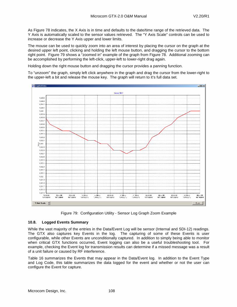
Microcom GTX-2.0 O&M Manual V2.20/R1
Microcom Design, Inc. 108
As Figure 78 indicates, the X Axis is in time and defaults to the date/time range of the retrieved data. The Y Axis is automatically scaled to the sensor values retrieved. The “Y Axis Scale” controls can be used to increase or decrease the Y Axis upper and lower limits.
The mouse can be used to quickly zoom into an area of interest by placing the cursor on the graph at the desired upper left point, clicking and holding the left mouse button, and dragging the cursor to the bottom right point. Figure 79 shows a “zoomed in” example of the graph from Figure 78. Additional zooming can be accomplished by performing the left-click, upper-left to lower-right drag again.
Holding down the right mouse button and dragging the cursor provides a panning function.
To “unzoom” the graph, simply left click anywhere in the graph and drag the cursor from the lower-right to the upper-left a bit and release the mouse key. The graph will return to it’s full data set.
Figure 79: Configuration Utility - Sensor Log Graph Zoom Example
10.8. Logged Events Summary
While the vast majority of the entries in the Data/Event Log will be sensor (Internal and SDI-12) readings. The GTX also captures key Events in the log. The capturing of some of these Events is user configurable, while other Events are unconditionally captured. In addition to simply being able to monitor when critical GTX functions occurred, Event logging can also be a useful troubleshooting tool. For example, checking the Event log for transmission results can determine if a missed message was a result of a unit failure or caused by RF interference.
Table 16 summarizes the Events that may appear in the Data/Event log. In addition to the Event Type and Log Code, this table summarizes the data logged for the event and whether or not the user can configure the Event for capture.

Microcom GTX-2.0 O&M Manual V2.20/R1
Microcom Design, Inc. 109
The “STX” and “ETX” Events are tied to transmissions. The “STX” Event simply logs the type of transmission and reports it as an ASCII string. Test transmissions are always logged, while Timed and Random transmission can be selectively logged. The “ETX” logs the result of the transmission. For good transmission three values are captured (battery volts, forward power, and reflected power). For failed transmissions a failure code string is reported (see Section 11.10.6 for the possible types of failures).
Two types of GPS related events can be logged (i.e. “SYNC” or “TCXO”). The “SYNC” event identifies when the GTX’s internal clock was last synchronized using the GPS receiver; the data captured for this event is the number of seconds the internal clock differed from UTC prior to the synchronization; the value is reported with a resolution of one millisecond. The “TCXO” Event marks when the units oscillators were re-calibrated using the GPS receiver, and log the absolute error from the expected nominal in parts per million.
The next sequence of Events listed in Table 16 refer to when the GTX itself is enabled or disabled, and when Self Timed and/or Random transmission are enabled or disabled. For each of these Events, the data reported is an ASCII string describing the Event.
The last Event listed in Table 16 is an Equation Constant change. This event is logged whenever the user alters one of the sixty-four configurable equation constants, with the GTX enabled. Changes to these constants can also be captured when the GTX is disabled, but the user must explicitly request the logging to occur (see Section 11.6.3 for details). The Log Code is the user defined Label for the Configuration Constant that was changed, and the data captured is new value entered for the constant. See Section 7.1.2.2 for more information on configurable equation constants.
Event Type Log
Code
Data User
Config Start of Tx – Test STX “TEST” No Start of Tx – Timed STX “TIMED” Yes Start of Tx – Random STX “RANDOM” Yes End of Tx – Good ETX Battery Volts, Fwd Power, Rev Power Yes End of Tx – Bad ETX Failure Code – See Section 11.10.6 Yes GPS Time Sync SYNC Clock Error Prior to Sync in Seconds Yes GPS TCXO Calibration TCXO TCXO Frequency Error in ppm Yes GTX Disabled GTX “DIS” No GTX Enabled GTX “ENB” No GTX Enabled - Logger GTX “ENB LGR” No Timed Tx Disabled GTX “DIS ST-TX” No Timed Tx Enabled GTX “ENB ST-TX” No Random Tx Disabled GTX “DIS RN-TX” No Random Tx Enabled GTX “ENB RN-TX” No Equation Constant Label Value Assigned to Constant No
Table 16: Logged Events Summary

Microcom GTX-2.0 O&M Manual V2.20/R1
Microcom Design, Inc. 110
11. RS-232 Serial Port Interface Command Reference
All Data Entry, System Setup, Calibration, and Diagnostic functions are performed using an RS-232 Interface.
The Microcom GTX Utility Interface application (GUI) greatly reduces the complexity of configuring, monitoring, and deploying the Microcom GTX by providing an easy-to-use, graphical user interface. This interface application encapsulates all the commands detailed in this section.
The information provided in this section provides the user with the necessary information to perform GTX setup, control, and status monitoring from a host terminal (e.g. external data logger) or terminal application (i.e. when the GUI is not available).
11.1. RS-232 Command Protocol
The RS-232 port utilizes an ASCII command line interface allowing configuration via a terminal program, such as Windows HyperTerminal. The interface is also suitable for connection to data loggers equipped with an RS-232 port. By utilizing an ASCII command line interface (as opposed to a menu system), common configurations can be captured in a text editor and are readily downloadable.
11.1.1. RS-232 Interface Protocol
A [CR] (0x0d) must be entered to get the transmitter’s attention and is used to terminate a command line. The transmitter responds with a ‘>’ (0x3e) to indicate that it is ready to receive a command. If the transmitter is enabled for GOES transmissions and no command is entered for a period of time (default is 5 seconds, see Section 11.9.1), the transmitter’s attention is lost and another [CR] must be entered. Commands can optionally be terminated with [CR][LF]; in other words, a [LF] character received following a [CR] will be ignored.
Each character entered is echoed to the host to allow for simple error checking and to support the terminal nature of the implementation. A backspace character (BS, 0x08) deletes the last character entered. The ESC character (0x1b) will delete the entire command.
For commands that dump a significant amount of data, sending the ESC character (or pressing the ESC key when using a Terminal application) will immediately terminate the dump and cause the prompt character to be reported.
11.1.2. RS-232 Hardware Interface
The settings for the RS-232 port are 9600 BAUD, 8 data bits, no parity and 1 stop bit.
The serial port interface implements the RS-232 standard TXD, RXD, RTS, and CTS signals.
To conserve power during operation, the GTX will enter a sleep mode during idle periods. While the unit is in the low power mode, it monitors the RS-232 input lines and wakes up upon RTS going active or in response to a [CR] being received. If the unit is woken up due to the RTS line becoming active, it will activate the CTS line to signal that it is ready to receive data. If the unit is woken up due to the receipt of a [CR], CTS will be asserted and the prompt character (‘>’) will be issued.
11.1.3. RS-232 Command Format
With few exceptions, all commands use a three-character identifier. Command that do not utilize a three-character identifier are done to prevent them from being accidentally entered due to the nature of the command function. The three-character identifier is roughly an abbreviation or acronym of the command function. The commands described in the following sections will include the functional name with the three-character identifier or long name provided parenthetically. Note that while all three-character identifiers are shown in uppercase, the GTX will accept any combination of upper and lower case characters.
Many commands are used to set or retrieve various configuration/calibration parameters. When setting parameters, the command is followed by an equals sign (‘=’). When retrieving parameters, the command is followed by a question mark (‘?’).

Microcom GTX-2.0 O&M Manual V2.20/R1
Microcom Design, Inc. 111
Some commands are used to direct the transmitter to execute a specific function (e.g. clear a buffer); in such cases, neither a ‘=’ nor a ‘?’ is utilized. Although, some of these commands may allow an optional parameter that further defines what action(s) will be executed, in which case an equals sign will be necessary.
Where commands are only used to request status information, typically the question mark is optional; in other words, the status information will be returned regardless of whether or not the ‘?’ is included.
Unless otherwise noted, the transmitter will respond to all commands with …
OK[CR][LF]> if the command (and parameter) is (are) accepted.
ERR[CR][LF]> if a command or parameter is invalid, or if the command can not be accepted.
<cmd>=<data> when returning data parameters, <cmd> will match the command requesting [CR][LF]> the data.
11.1.4. RS-232 Access Rights
All commands are subject to an access right based on either the current state of the transmitter (enabled or disabled for GOES transmissions) or a password protection. Four levels of access rights are currently implemented. These are summarized below ordered from highest access required to lowest.
1. Development Access [dev]: Commands used for program debugging and/or NESDIS Certification.
2. Factory Access [fct]: Commands used for factory calibration and configuration. 3. Transmitter Disabled [dtx]: Commands used for operational configuration by end user. 4. Unrestricted [all]: Commands that may be issued at any time; typically status requests.
Development and Factory access commands are not intended for general use. As such, they are not covered in this document, and are password protected to prevent unauthorized use. Unauthorized use of these commands may cause the GTX to function incorrectly, and could violate NESDIS Certification.
Transmitter Disabled access commands are typically used for configuring the transmitter for GOES operation, and are controlled by the state of the transmitter. Commands to change/set these parameters are only allowed when the transmitter is disabled, i.e. GOES transmissions are disabled. If the transmitter is enabled, then only the query form of the command is allowed.
The access level for each command is provided in brackets in the section title using the codes shown in the list above.
11.1.5. Password Protection for Configuration Comma nds
In addition to having an access level of “dtx”, commands that affect the GTX’s configuration setup (e.g. transmissions, sensors, data formatting, etc.) are also password protected to prevent unauthorized access, especially in a remote access (e.g. modem) situation. The configuration password can be set and/or edited by the CPW command (see Section 11.9.8).
Once a GTX has been enabled for operation, changing the configuration requires the user to place the unit in the disabled state (DTX), followed by entering the password using the CPE command (see Section 11.9.7). Until the configuration is “unlocked” by entering the correct password, the configuration cannot be edited or modified, and the response to any configuration command will be ERR. The Microcom GTX Configuration Utility also supports the use of password protection for the configuration.
If the password is not entered or explicitly cleared, then it is not necessary to utilize the CPE command to unlock the configuration. However, disabling the GTX is always required.
Further, note that the password protection does not take affect until the unit has been enabled at least once. As such, entering the password does not immediately lock the configuration to facilitate initial field deployment.
If the configuration password is entered incorrectly or is otherwise unknown to the user (e.g. forgotten), then it is still possible to “unlock” the GTX. However to do so requires recycling the power and not entering the enabled state. As such, the Power Up Enable (PUE) and Configuration Save (CFS)

Microcom GTX-2.0 O&M Manual V2.20/R1
Microcom Design, Inc. 112
commands (see Sections 11.3.9 and 11.9.2, respectively), are the only configuration commands that are not password protected. Therefore, to unlock a GTX without knowing the password requires the following 5 step process:
1. Disable the GTX (DTX). 2. Disable power up enables (PUE=0). 3. Save the configuration (CFS) – only updates the PUE flag, since all other configuration
commands are protected. 4. Turn the GTX off; requires physically disconnecting power. 5. Turn the GTX on; reconnect power. The GTX will power up in the disabled state and will not
require password unlocking.
Note that the approach outlined above requires being physically present at the GTX and is not possible to accomplish remotely. Further, this approach avoids the use of a permanent “hidden” or “backdoor” password being hard-coded in the GTX firmware; which once known could be used to unlock any GTX.
11.2. Satellite Transmission Configuration Commands
The following commands are used to set the configuration parameters for GOES transmissions. Unless otherwise specified, these parameters have invalid default values and must be set explicitly before transmissions can be enabled using the Enable GTX (ETX) command. These parameters are stored in nonvolatile memory by issuing the Configuration Save (CFS) command (see Section 11.9.2) or will be automatically saved when the transmitter is enabled.
The transmitter must be explicitly disabled using the DTX command before these parameters can be modified. Parameters can be read by entering ’?’ in place of the value in the command string while transmissions are enabled or disabled. All parameters can be read at the same time using the Read Configuration (RCF) command.
11.2.1. Platform ID (PID=xxxxxxxx) [dtx]
This command sets the Platform ID (i.e. the NESDID GOES DCP ID) command to value xxxxxxxx. Valid range is 0x00000002 to 0xFFFFFFFE (4 byte, 8 Hex characters), and only even values will be accepted.
Setting PID=INV will clear the current Platform ID and return it to an invalid state.
11.2.2. GTX Operation Mode (GTX=x) [dtx]
This command accepts/returns a single numerical value in the range of 0 to 6 that determines/identifies the operational mode of the GTX-2.0. Among other things, the operational mode specifies the transmitter modulation and data rate, and the satellite system channel designations.
Operational Mode
Value
Mode Notes
Date Rate(s)
Logger Only 0 No Transmit Functions are Enabled N/A NOAA GOES 1 Default – Channels per Version 2 Spec 300,1200 MeteoSat/EumetSat 2 MeteoSat 2ND Generation Channels 100 ARGOS 3 ARGOS Channels – Random Only 400 ARGOS/SCD 4 ARGOS & SCD Channels – Random Only 400 INSAT PBRS 5 INSAT Pseudo Random Burst Mode 4800 INSAT TDMA 6 INSAT Self-Timed (reserved for future) 4800
Table 17: GTX-2.0 Operational Modes
11.2.3. Timed Transmit Channel (TCH=ccc,bbbb) [dtx]
This command sets the channel number (ccc ) and bit rate (bbbb ) for timed transmissions.
The allowable channel number (ccc ) and bit rate (bbbb) parameters depend on the GTX Mode.
Setting the channel number to 0 will disable timed transmissions; when disabling timed transmissions, the bit rate parameter is not required.

Microcom GTX-2.0 O&M Manual V2.20/R1
Microcom Design, Inc. 113
11.2.4. Timed Transmit Interval (TTI=dd:hh:mm:ss) [ dtx]
This command sets the interval between timed transmissions to days, hours, minutes, seconds specified in dd:hh:mm:ss. Valid range is 00:00:05:00 to 30:00:00:00.
Default value is 00:01:00:00, or once an hour.
11.2.5. First Transmission Time (FTT=hh:mm:ss) [dtx ]
This command sets the time for the first timed transmission of the day. While the TTI command sets the interval of the transmissions, the FTT command essentially sets where in the interval the transmission will occur. Valid range is 00:00:00 to 23:59:59.
NOTE: The time of first transmission MUST always be entered in UTC (aka. GMT) even if the GTX is configured to operate in local time (see Sections 11.3.2 and 11.3.5). The GTX will automatically adjust the actual time of the first transmission to local time, if necessary.
Default value is 00:00:00.
11.2.6. Timed Window Length (TWL=xxx) [dtx]
This command sets the length of the timed transmit window. Length is specified in seconds. Valid range is 5 to 240 seconds. Note that the maximum window length can exceed the failsafe limits.
Default value is 30 seconds.
11.2.7. Timed Operation Flags (TOF=xx) [dtx]
This command sets the option byte for timed transmissions. The timed option byte is a bit-mapped value that determines various operation modes for timed transmissions. The value must be entered in a hexadecimal format.
The default value for the TimedOpFlags is all bits cleared.
The bit mapping is provided in the table below; unused bits should be set to 0.
Bit Name Description 0 Window Position 0 = Message aligned at top of Timed Window.
1 = Message aligned to center of Timed Window. 1 Buffer Dump 0 = Do not dump Timed Buffer.
1 = Dump Timed Buffer to RS-232 after Tx. 2 Status Dump 0 = Do not dump Timed status.
1 = Dump Timed status to RS-232 after Tx. 3 Log TX Start 0 = Do not log start of Timed Tx in Data/Event buffer.
1 = Log start of Timed Tx in Data/Event buffer. 4 Log TX End 0 = Do not log end of Timed Tx in Data/Event buffer.
1 = Log end of Timed Tx and stats in Data/Event buffer. 5 Not used Reserved for future use 6 Buffer Empty 0 = Send null data if Timed Buffer empty.
1 = Send “BUFFER EMPTY” if no Timed data. 7 No Clear 0 = Timed Buffer cleared after transmission.
1 = Timed Buffer not cleared after transmission.
Table 18: Timed Operation Flag Byte
11.2.8. Timed Preamble (TPR=xxxxx) [dtx]
This command sets the preamble type for timed transmissions. Valid values are Short or Long (a.k.a. S or L). This setting only applies to METEOSAT 100 bps timed transmissions.
Default value is Short.

Microcom GTX-2.0 O&M Manual V2.20/R1
Microcom Design, Inc. 114
11.2.9. Timed Data Format (TDF=xxxxxx) [dtx]
This command sets the timed transmission data format to ASCII, Pseudo (pseudo-binary), or Binary (a.k.a. A, P or B).
When the Timed Data Source (TDS) is set to RS-232, this parameter is used to set the flag word in a GOES transmission.
When the Timed Data Source is set to Sensor, this parameter is used to determine the formatting of sensor data before it is stored in the transmit buffer. Currently a timed format of Binary is not valid when the timed data source is Sensor.
Default value is ASCII.
11.2.10. Timed Data Source (TDS=xxxxxx) [dtx]
This command sets the source for data for timed transmissions. Valid values are RS-232 or Sensor (a.k.a. R or S). When set to RS-232, the transmitter accepts data for transmission from the RS-232 port via the TDT command. When set to Sensor, the transmitter will collect, format, and store sensor parameter in the Timed Transmit buffer.
Default value is RS-232.
11.2.11. Timed Data Order (TDO=xxxxxx) [dtx]
The Timed Data Order is a global value that determines the order in which multiple data points from the same parameter are stored in the Timed buffer. This value can be set to Newest (a.k.a. N), which indicates the most recent data point will be transmitted first (i.e. newest-to-oldest); or it can be set to Oldest (a.k.a. O), which indicates the oldest data point will be transmitted first (i.e. oldest-to-newest). This parameter is only applicable when TDS=SENSOR.
Default value is Newest.
11.2.12. Random Transmit Channel (RCH=ccc,bbbb) [dt x]
This command sets the channel number (ccc ) and bit rate (bbbb ) for random transmissions.
The allowable channel number (ccc ) and bit rate (bbbb) parameters depend on the GTX Mode.
Setting the channel number to 0 will disable random transmissions; when disabling random transmissions, the bit rate parameter is not required.
11.2.13. Random Transmit Interval (RIN=xxx) [dtx]
This command sets the random transmission interval. The randomizing interval is the interval in which a random transmission will occur once a random report has been triggered. The actual transmission time will be random, but on average will occur at this rate.
For GOES operation, xxx is in minutes, and the valid range is 5 to 99 minutes.
Default value is 15 minutes.
11.2.14. Randomization Percent (RPC=pp) [dtx]
This command sets the random transmission randomizing percentage. This value determines the range of randomization as a percentage of the Random Interval (RIN). Random transmissions will occur at a uniformly distributed random time within this range and on average occur at the Random Interval rate. Valid range is 10 to 50%.
Default value is 20%
For example, for a Random Interval of 15 minutes and a Random Percent of 20%, then the time between any two random transmissions will be 12 to 18 minutes (15 ± 3 minutes).

Microcom GTX-2.0 O&M Manual V2.20/R1
Microcom Design, Inc. 115
11.2.15. Random Repeat Count (RRC=xx) [dtx]
This command sets the random transmission repeat count. The random transmission repeat count is the number of times a random transmission will be repeated before the sequence of Random reports is terminated. Random transmissions will occur once every random transmission interval as specified by the Random Interval (RIN) parameter. The valid range of this parameter is 0 – 99.
For example, a value of 3 will direct the transmitter to send the data in the Random buffer 3 times before terminating.
A value of 0 indicates that random transmissions will occur every random transmission interval until explicitly terminated by the host.
When the Random Data Source is set to RS-232, random reports are only triggered in response to data being loaded into the buffer via the RDT command. Upon completion of the programmed number of random transmissions, the Random buffer will be automatically cleared and the random transmission sequence terminated. When RRC=0, random transmissions will continue until the host clears the Random buffer.
When the Random Data Source is set to Sensor, random reports are triggered in response to user configurable set points based on the data being collected. In Sensor mode, data is continuously being collected and stored in the Random buffer based on the user’s setup; therefore, upon completion of the programmed number of random transmissions, the Random buffer is not cleared when the random transmission sequence terminated. In this mode when RRC=0, random transmissions will begin immediately once the GTX is enabled (ETX) and will continue as long the unit remains in this state, i.e. the host must explicitly disables the GTX using the DTX to terminate random transmissions.
Default value is 3.
11.2.16. Random Data Format (RDF=xxxxxx) [dtx]
This command sets the random transmission data format to ASCII, Pseudo (pseudo-binary), or Binary (a.k.a. A, P or B).
When the Random Data Source is set to RS-232, this parameter is used to set the flag word in GOES 300 and 1200 bps transmissions.
When the Random Data Source is set to Sensor, this parameter is used to determine the formatting of sensor data before it is stored in the transmit buffer.
Default value is Pseudo.
11.2.17. Random Data Source (RDS=xxxxxx) [dtx]
This command sets the source for data for random transmissions. Valid values are RS-232 or Sensor (a.k.a. R or S). When set to RS-232, the transmitter accepts data for transmission from the RS-232 port via the RDT command. When set to Sensor, the transmitter will collect, format, and store sensor parameter in the Random Transmit buffer.
Default value is RS-232.
11.2.18. Random Data Order (RDO=xxxxxx) [dtx]
The Random Data Order is a global value that determines the order in which multiple data points from the same parameter are stored in the Random buffer. This value can be set to Newest (a.k.a. N), which indicates the most recent data point will be transmitted first (i.e. newest-to-oldest); or it can be set to Oldest (a.k.a. O), which indicates the oldest data point will be transmitted first (i.e. -to-oldest-to-newest). This parameter is only applicable when RDS=SENSOR.
Default value is Newest.
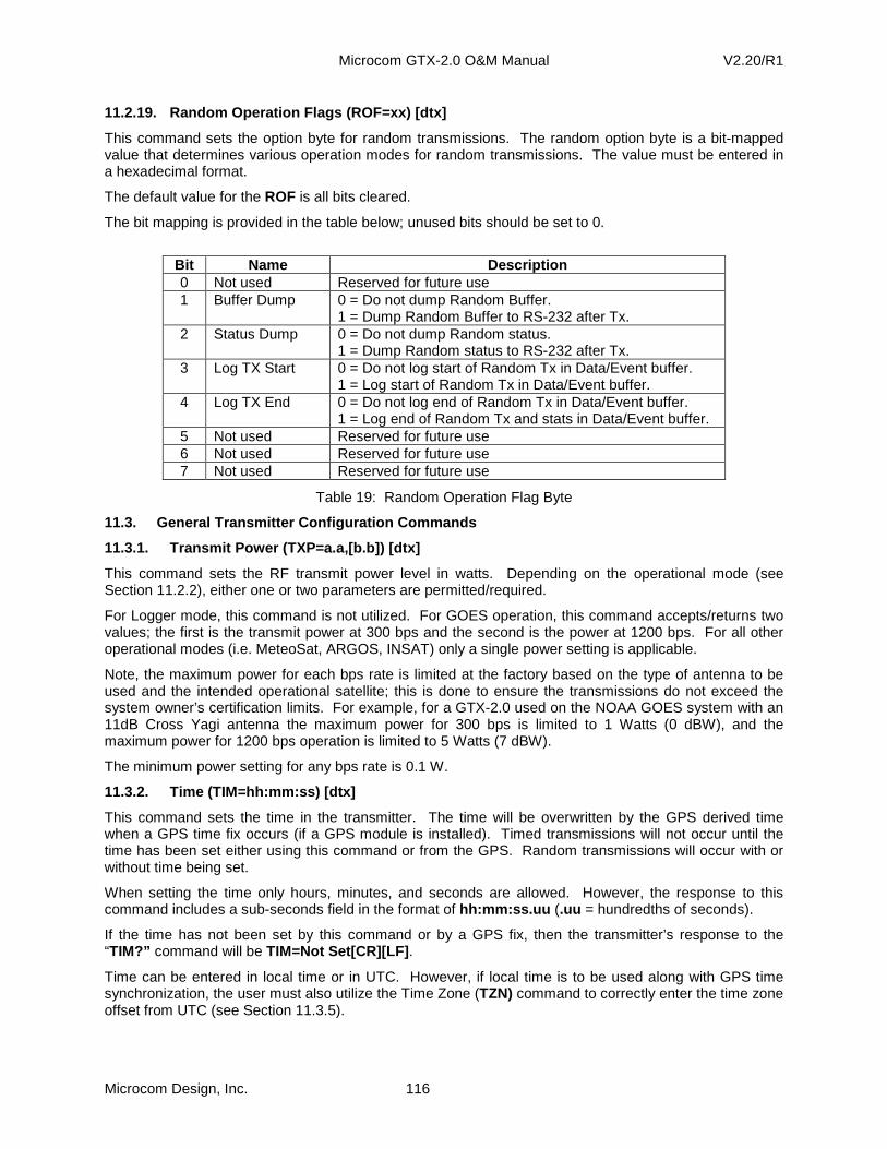
Microcom GTX-2.0 O&M Manual V2.20/R1
Microcom Design, Inc. 116
11.2.19. Random Operation Flags (ROF=xx) [dtx]
This command sets the option byte for random transmissions. The random option byte is a bit-mapped value that determines various operation modes for random transmissions. The value must be entered in a hexadecimal format.
The default value for the ROF is all bits cleared.
The bit mapping is provided in the table below; unused bits should be set to 0.
Bit Name Description 0 Not used Reserved for future use 1 Buffer Dump 0 = Do not dump Random Buffer.
1 = Dump Random Buffer to RS-232 after Tx. 2 Status Dump 0 = Do not dump Random status.
1 = Dump Random status to RS-232 after Tx. 3 Log TX Start 0 = Do not log start of Random Tx in Data/Event buffer.
1 = Log start of Random Tx in Data/Event buffer. 4 Log TX End 0 = Do not log end of Random Tx in Data/Event buffer.
1 = Log end of Random Tx and stats in Data/Event buffer. 5 Not used Reserved for future use 6 Not used Reserved for future use 7 Not used Reserved for future use
Table 19: Random Operation Flag Byte
11.3. General Transmitter Configuration Commands
11.3.1. Transmit Power (TXP=a.a,[b.b]) [dtx]
This command sets the RF transmit power level in watts. Depending on the operational mode (see Section 11.2.2), either one or two parameters are permitted/required.
For Logger mode, this command is not utilized. For GOES operation, this command accepts/returns two values; the first is the transmit power at 300 bps and the second is the power at 1200 bps. For all other operational modes (i.e. MeteoSat, ARGOS, INSAT) only a single power setting is applicable.
Note, the maximum power for each bps rate is limited at the factory based on the type of antenna to be used and the intended operational satellite; this is done to ensure the transmissions do not exceed the system owner’s certification limits. For example, for a GTX-2.0 used on the NOAA GOES system with an 11dB Cross Yagi antenna the maximum power for 300 bps is limited to 1 Watts (0 dBW), and the maximum power for 1200 bps operation is limited to 5 Watts (7 dBW).
The minimum power setting for any bps rate is 0.1 W.
11.3.2. Time (TIM=hh:mm:ss) [dtx]
This command sets the time in the transmitter. The time will be overwritten by the GPS derived time when a GPS time fix occurs (if a GPS module is installed). Timed transmissions will not occur until the time has been set either using this command or from the GPS. Random transmissions will occur with or without time being set.
When setting the time only hours, minutes, and seconds are allowed. However, the response to this command includes a sub-seconds field in the format of hh:mm:ss.uu (.uu = hundredths of seconds).
If the time has not been set by this command or by a GPS fix, then the transmitter’s response to the “TIM?” command will be TIM=Not Set[CR][LF] .
Time can be entered in local time or in UTC. However, if local time is to be used along with GPS time synchronization, the user must also utilize the Time Zone (TZN) command to correctly enter the time zone offset from UTC (see Section 11.3.5).
Microcom GTX-2.0 O&M Manual V2.20/R1
Microcom Design, Inc. 117
11.3.3. Date (DAT=mm/dd/yyyy) [dtx]
This command sets the date in the transmitter. The date will be overwritten by the GPS derived date when a GPS fix is acquired (if a GPS module is installed). Timed transmissions will not occur until the date has been set either using this command or from the GPS. Random transmissions will occur with or without the date being set.
If the date has not been set by this command or by a GPS fix, then the transmitter’s response to the “DAT?” command will be DAT=Not Set[CR][LF] .
11.3.4. Time Correct (TIC) [all]
This Time Correct command allows the time to be corrected for drift errors without re-entering the time. Note that this command is valid at any time (provided the time and date have been set), so it can be utilized to correct the time without disabling the GTX.
This command neither accepts nor returns any parameters. Issuing the command directs the GTX to reset its internal clock to the nearest minute. In other words, if the current time is within the first half of a minute (seconds < 30), then this command simply zeroes out the seconds; if the current time is in the second half of the minute (seconds >= 30), then the GTX advances the clock (time and date) to the top of the next minute.
11.3.5. Time Zone Offset (TZN) [dtx]
The Time Zone Offset command allows the user to enter a time zone correction in hours relative to UTC. Entering a time zone correction is absolutely necessary if the GTX is to be operated in local time with GPS time synchronization possible. While the time in the GTX can be manually entered, using GPS to update the clock will cause the time to be reset automatically when the GTX performs a time sync. However, prior to applying the update, the GTX will adjust the UTC time provided by the GPS receiver by the time zone correction to convert UTC to local time.
The time zone correction can be set in the range of -13 to +13 hours in quarter hour steps (0.25). Setting the value to 0, implies the GTX is working in UTC or GMT.
Default value is 0.
11.3.6. UTC Correction (UTC) [all]
The UTC command allows the user to preset or request the UTC correction. The UTC correction is an integer offset in seconds from GPS time to UTC or GMT. While the GPS receiver will automatically determine the offset from the GPS satellites, the correction factor is only sent once every 12.5 minutes. As such, this command can be used to preset the offset value, which can greatly speed up the time to synchronize the GTX’s internal clock. As of July 1, 2012, the UTC correction is -16 seconds.
As a preset, this is a “one-time use only” setting, i.e. the next time the GTX synchronizes the clock via the GPS receiver it will wait until the correction is received.
To preset the offset correction, the command format is UTC=-16. Note that this command has an access level of all , so it can be used even after the GTX has been enabled. Once the GTX obtains the correction from the GPS system, it will not accept a preset value.
Issuing the query form of this command (UTC?) can produce one of three responses. If the UTC correction has not been determined from the GPS system and has not been preset by the user, the GTX will respond with UTC=Not Set . If the UTC correction has been set by GPS, the response will be UTC=-16,G. If the UTC correction has been manually preset, the response is UTC=-16,M.
11.3.7. Invalid Replace Character (IRC=c) [dtx]
This command defines the ASCII character that will be substituted for any invalid character detected in a transmission buffer. Certain operational modes (e.g. GOES Pseudo-Binary, METEOSAT International, etc.) restrict the allowable characters that can be transmitted. If the GTX is operating in one of these modes and detects a prohibited character in the transmission buffer, it will transmit this character in its place. The default character is the forward slash ‘/’. Only printable ASCII characters (space through tilde) are permitted.

Microcom GTX-2.0 O&M Manual V2.20/R1
Microcom Design, Inc. 118
11.3.8. Slash Fill (SFL=b) [dtx]
The Slash Fill command controls how unread data fields in transmission buffers are filled. The default configuration for the GTX is to fill the fields with ASCII space characters on buffer initialization. Setting this parameter to 1 (SFL=1), directs the GTX to use the ASCII slash character (/) as the fill character.
Once the GTX is enabled, as sensor data is read and processed the captured data will overwrite the fill characters. However, if a sensor fails, the GTX will apply fill data to the field to distinguish between an actual reading and an error.
With this flag set to 0, the GTX will fill Pseudo-Binary fields with spaces in the event of an erroneous reading. For ASCII transmission, the GTX will insert the string ‘‘N/M” along with enough space to fill the fieldwidth to indicate “No Measurement”; if the fieldwidth is less than 4 characters, the GTX will only fill spaces.
When SFL=1, transmission fields will instead simply be filled with the slash character in the event of erroneous readings.
Note that when slash filling is utilized for ASCII transmission fields, the left most character of the field will still be a space to delimit the field. However, Pseudo-Binary transmission fields are always completely filled.
Default value is 0. (No slash fill).
11.3.9. Power Up Enabled (PUE=b) [dtx]
This command directs the transmitter to power up enabled (b=1) or disabled (b=0). Setting this flag to true (b=1) can be used to avoid having to explicitly enable the unit during field deployment. If the transmitter is configured for its operational mode, then setting this flag true (and saving it with the configuration), will cause the unit to immediately enter the enabled state upon power up.
If the transmitter is configured for timed transmission operation or no BBU-RTC is available in the unit, an immediate GPS fix will be initiated on power up. Note that if a GPS receiver is not installed, this mode can still be used if a BBU-RTC is available and the transmitter is only configured for random reports or for use as a logger only.
Clearing this flag directs the unit to power up into the disabled state. This command is only one of two configuration commands that are not password protected (see Section 11.1.5).
Default value is 0. (Power Disabled).
11.4. RS-232 Transmit Data Storage Commands
The following commands are used to manage and store data in the transmission buffers using the RS-232 port as the source for data.
11.4.1. Literal Character Designator, ‘/’
When using the RS-232 buffer to load data into a transmit buffer, certain bytes or characters must be preceded with a literal character slash (‘/’) to avoid being misinterpreted as a command control character. For example, if a [CR] is to be loaded into the Timed (TDT) or Random (RDT) buffer, then the [CR] must be preceded with the literal character since the [CR] (0x0d) character is used to indicate the end of a data storage command (as with other command types).
The only other two command control characters used by the transmitter are [BS] (0x08, used to edit commands) and [ESC] (0x1b, used to terminate commands). Accordingly, to load these binary values into a transmit buffer also requires use of the literal designator.
In actuality, except for a few special cases, receipt of the literal character (‘/’) will direct the transmitter to load the next character as it is received into the buffer. Therefore, to actually load a slash character into the desired buffer requires sending two consecutive slashes, i.e. ‘//’.
Three special cases have been implemented in the interface to facilitate loading the characters listed below when operating the transmitter from a terminal program (e.g. for test and troubleshooting).
Microcom GTX-2.0 O&M Manual V2.20/R1
Microcom Design, Inc. 119
• /R or /r will load a [CR] (0x0d)
• /N or /n will load a [LF] (0x0d)
• /T or /t will load a [HT] (0x09)
However, when the transmitter is connected to an autonomous host (e.g. a data logger), it is not necessary to precede any binary characters other than those that correlate to those specified above ([CR], [BS], [ESC], and ‘/’) with the literal designator.
11.4.2. Timed Data Buffer Load (TDT=xxx…) [etx]
The TDT command appends host formatted data to the Timed buffer when the Timed Data Source is RS-232. This command is not permitted and will return an error response (ERR) when TDS=SENSOR, or whenever the transmitter is disabled.
Prior to sending a timed transmission, the transmitter will insert the appropriate preamble and programmed DCP ID, any header information (e.g. HDR flag byte and/or sequence number), and for GOES operation append the appropriate EOT. If the Timed Data Format (TDF) is ASCII or Pseudo-Binary the transmitter will also insert the correct parity bit for each message character.
The maximum length of the formatted data can be up to 126000 bits, or 15750 bytes (see Section 1.2.3.2.1). However, the actual buffer size is calculated based on the Timed Window Length (TWL), i.e. the transmitter will not accept more bytes than can be sent in the programmed window length at the configured bps format.
If this command is received when a transmission is initiated and pending (approximately 5 seconds before the scheduled transmission) or during a timed transmission, the data will not be included in the current transmission but will be buffered for the next timed transmission. When a timed transmission is complete, the transmitted data will be automatically cleared from the timed buffer unless the “No Clear” flag is set (see Section 11.2.7).
The transmitter responds with: [CR][LF]> if the data is accepted. ERR[CR][LF]> if the buffer is full
Note that the transmitter will not prevent any prohibited characters from being loaded into the buffer. Instead, these characters will be replaced with a user defined character before being transmitted if the unit is configured for Pseudo-Binary operation.
The unique nature of this command requires that several important distinctions from other commands be noted.
• This command will only be accepted when the transmitter is enabled.
• Once the equals sign is received, the command itself may not be edited. In other words, backspacing to the point where the equals sign is deleted will terminate the command.
• While other commands have a predetermined number of parameters, the amount of data that can be loaded with this command is only limited by the buffer size as determined by the transmit window length.
11.4.3. Timed Buffer Size (TBS?) [all]
This command returns the number of bytes stored in the timed transmission buffer.
11.4.4. Clear Timed Buffer (CTB) [all]
This command clears the timed transmission buffer if the Timed data source is the RS-232 port. The command has no effect when TDS=SENSOR.
11.4.5. Timed Buffer Dump (TBD) [all]
The TBD command will dump the current contents of the Timed transmit buffer. This command can be used to verify that data collected from sensors is properly formatted and loaded into the timed transmission buffer. In addition to the actual data stored in the buffer, this command also reports the number of bytes stored in the timed buffer as shown in the example below.
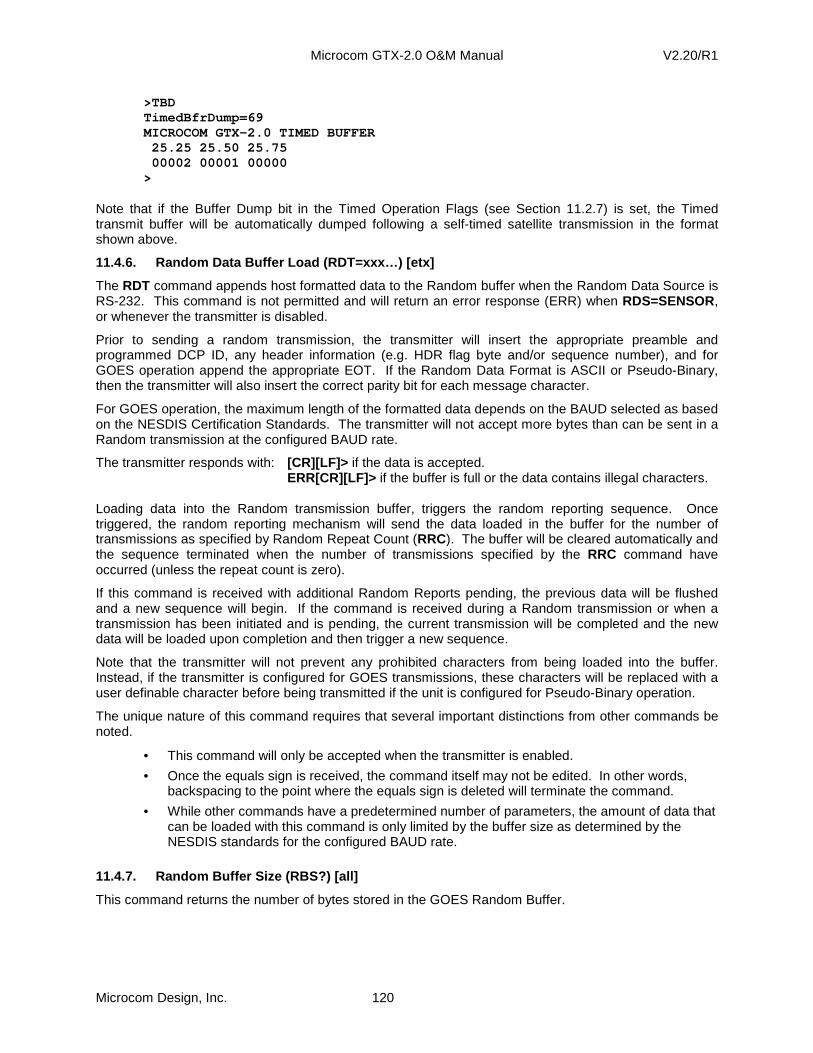
Microcom GTX-2.0 O&M Manual V2.20/R1
Microcom Design, Inc. 120
>TBD TimedBfrDump=69 MICROCOM GTX-2.0 TIMED BUFFER 25.25 25.50 25.75 00002 00001 00000 >
Note that if the Buffer Dump bit in the Timed Operation Flags (see Section 11.2.7) is set, the Timed transmit buffer will be automatically dumped following a self-timed satellite transmission in the format shown above.
11.4.6. Random Data Buffer Load (RDT=xxx…) [etx]
The RDT command appends host formatted data to the Random buffer when the Random Data Source is RS-232. This command is not permitted and will return an error response (ERR) when RDS=SENSOR, or whenever the transmitter is disabled.
Prior to sending a random transmission, the transmitter will insert the appropriate preamble and programmed DCP ID, any header information (e.g. HDR flag byte and/or sequence number), and for GOES operation append the appropriate EOT. If the Random Data Format is ASCII or Pseudo-Binary, then the transmitter will also insert the correct parity bit for each message character.
For GOES operation, the maximum length of the formatted data depends on the BAUD selected as based on the NESDIS Certification Standards. The transmitter will not accept more bytes than can be sent in a Random transmission at the configured BAUD rate.
The transmitter responds with: [CR][LF]> if the data is accepted. ERR[CR][LF]> if the buffer is full or the data contains illegal characters.
Loading data into the Random transmission buffer, triggers the random reporting sequence. Once triggered, the random reporting mechanism will send the data loaded in the buffer for the number of transmissions as specified by Random Repeat Count (RRC). The buffer will be cleared automatically and the sequence terminated when the number of transmissions specified by the RRC command have occurred (unless the repeat count is zero).
If this command is received with additional Random Reports pending, the previous data will be flushed and a new sequence will begin. If the command is received during a Random transmission or when a transmission has been initiated and is pending, the current transmission will be completed and the new data will be loaded upon completion and then trigger a new sequence.
Note that the transmitter will not prevent any prohibited characters from being loaded into the buffer. Instead, if the transmitter is configured for GOES transmissions, these characters will be replaced with a user definable character before being transmitted if the unit is configured for Pseudo-Binary operation.
The unique nature of this command requires that several important distinctions from other commands be noted.
• This command will only be accepted when the transmitter is enabled.
• Once the equals sign is received, the command itself may not be edited. In other words, backspacing to the point where the equals sign is deleted will terminate the command.
• While other commands have a predetermined number of parameters, the amount of data that can be loaded with this command is only limited by the buffer size as determined by the NESDIS standards for the configured BAUD rate.
11.4.7. Random Buffer Size (RBS?) [all]
This command returns the number of bytes stored in the GOES Random Buffer.

Microcom GTX-2.0 O&M Manual V2.20/R1
Microcom Design, Inc. 121
11.4.8. Clear Random Buffer (CRB) [all]
This command clears the random transmission buffer if the Random data source is the RS-232 port. In this mode, clearing the random transmission buffer will also terminate the active Random Report sequence. The command has no effect when RDS=SENSOR.
11.4.9. Random Buffer Dump (RBD) [all]
The RBD command will dump the current contents of the Random transmit buffer. This command can be used to verify that data collected from sensors is properly formatted and loaded into the timed transmission buffer. In addition to the actual data stored in the buffer, this command also reports the number of bytes stored in the timed buffer as shown in the example below.
>RBD RBD=17 Acg]gvhO@@B@@A@@@ >
Note that if the Buffer Dump bit in the RandomOpFlags (see Section 11.2.19) is set, the Random transmit buffer will be automatically dumped following a self-timed satellite transmission in the format shown above.
11.4.10. Random Buffer Transmissions Remaining (RBT ) [all]
This command returns the number of Random transmissions remaining to be sent in the current Random Report sequence. If the transmitter or Random Reports are not enabled, the command returns ‘N/A’. If the Random Repeat Count is set to zero, then the command returns ‘Inf’, indicating the Random Reports will continue until the host clears the Random Buffer.
11.5. Data Collection Setup and Test Commands
The GTX’s capabilities also include being able to collect, process, format, store, and transmit data from external SDI-12 devices as well as its internal sensor functions. This extended functionality allows the GTX to be used as a complete DCP without the need for an external Data Logger. It also allows the GTX to operate as a standalone Data Logger.
Setting the GTX up to collect and transmit data is a relatively simple, two-step process. First, the user must configure the actual data collection. Second, the user must configure the desired transmit buffer to format and log the data for transmission.
By separating these functions, it is possible to have the data captured from a sensor to be stored in either the Timed buffer, the Random buffer, both buffers, or neither, but be used to trigger Random Reports. Further, not only can the same data be stored in both buffers, it’s also possible to store it in different formats; e.g. ASCII in the Timed buffer, and Pseudo-Binary in the Random buffer. Sampled data is also passed to the equation processor, the Min, Max, Average (MMA) processor and the Data/Event log.
The following subsections detail the commands used to configure and test the data collection functions. Section 11.6 details the commands to format and log data into the transmit buffers.
11.5.1. SDI-12 Data Collection Setup and Test Comma nds
The following sections detail the SDI-12 data collection setup and test commands implemented in the GTX. Up to 64 SDI-12 parameters can be collected and stored by the GTX. These parameters can be collected from a single SDI-12 device or from multiple SDI-12 devices. As the parameters are collected, they are passed to the data format and storage module where they can be included in the Timed or Random transmission buffer (or both). The SDI-12 parameters can also be used to trigger random reports, operated on by the equation and MMA processors, and stored in the Data/Event log.
While an absolute maximum of 64 SDI-12 parameters can be defined and collected, the actual number of SDI-12 parameters that can implemented depends on the Soft Configuration of the GTX (see Section 5).
To allow maximum flexibility, the configuration of the SDI-12 data collection is independent of the data storage functions. In other words, the commands described in the following subsections only define what
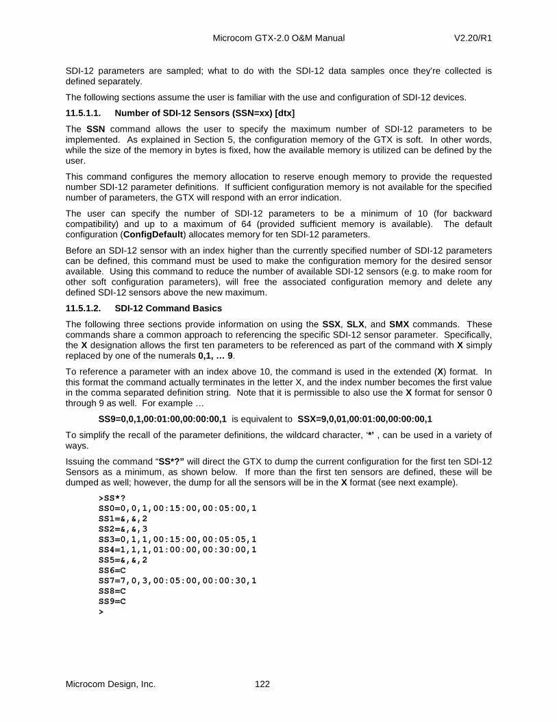
Microcom GTX-2.0 O&M Manual V2.20/R1
Microcom Design, Inc. 122
SDI-12 parameters are sampled; what to do with the SDI-12 data samples once they’re collected is defined separately.
The following sections assume the user is familiar with the use and configuration of SDI-12 devices.
11.5.1.1. Number of SDI-12 Sensors (SSN=xx) [dtx]
The SSN command allows the user to specify the maximum number of SDI-12 parameters to be implemented. As explained in Section 5, the configuration memory of the GTX is soft. In other words, while the size of the memory in bytes is fixed, how the available memory is utilized can be defined by the user.
This command configures the memory allocation to reserve enough memory to provide the requested number SDI-12 parameter definitions. If sufficient configuration memory is not available for the specified number of parameters, the GTX will respond with an error indication.
The user can specify the number of SDI-12 parameters to be a minimum of 10 (for backward compatibility) and up to a maximum of 64 (provided sufficient memory is available). The default configuration (ConfigDefault ) allocates memory for ten SDI-12 parameters.
Before an SDI-12 sensor with an index higher than the currently specified number of SDI-12 parameters can be defined, this command must be used to make the configuration memory for the desired sensor available. Using this command to reduce the number of available SDI-12 sensors (e.g. to make room for other soft configuration parameters), will free the associated configuration memory and delete any defined SDI-12 sensors above the new maximum.
11.5.1.2. SDI-12 Command Basics
The following three sections provide information on using the SSX, SLX, and SMX commands. These commands share a common approach to referencing the specific SDI-12 sensor parameter. Specifically, the X designation allows the first ten parameters to be referenced as part of the command with X simply replaced by one of the numerals 0,1, … 9.
To reference a parameter with an index above 10, the command is used in the extended (X) format. In this format the command actually terminates in the letter X, and the index number becomes the first value in the comma separated definition string. Note that it is permissible to also use the X format for sensor 0 through 9 as well. For example …
SS9=0,0,1,00:01:00,00:00:00,1 is equivalent to SSX=9,0,01,00:01:00,00:00:00,1
To simplify the recall of the parameter definitions, the wildcard character, ‘*’ , can be used in a variety of ways.
Issuing the command “SS*?” will direct the GTX to dump the current configuration for the first ten SDI-12 Sensors as a minimum, as shown below. If more than the first ten sensors are defined, these will be dumped as well; however, the dump for all the sensors will be in the X format (see next example).
>SS*? SS0=0,0,1,00:15:00,00:05:00,1 SS1=&,&,2 SS2=&,&,3 SS3=0,1,1,00:15:00,00:05:05,1 SS4=1,1,1,01:00:00,00:30:00,1 SS5=&,&,2 SS6=C SS7=7,0,3,00:05:00,00:00:30,1 SS8=C SS9=C >

Microcom GTX-2.0 O&M Manual V2.20/R1
Microcom Design, Inc. 123
Issuing the command “SSX?” will direct the GTX to dump the current configuration for all defined sensors, but forces the X format even if only the first ten SDI-12 Sensors have definitions, as shown below.
>SSX? SSX=0,0,0,1,00:15:00,00:05:00,1 SSX=1,&,&,2 SSX=2,&,&,3 SSX=3,0,1,1,00:15:00,00:05:05,1 SSX=4,1,1,1,01:00:00,00:30:00,1 SSX=5,&,&,2 SSX=6,C SSX=7,7,0,3,00:05:00,00:00:30,1 SSX=8,C SSX=9,C >
Issuing the command “SS*=*?” or “SSX=*?” will direct the GTX to dump the current configuration for all available SDI-12 Sensors regardless of whether or not they are defined. In other words, the dump will include sensors 0 through one less than the value defined by SSN (since the indexing is zero based). For example, for the maximum number of SDI-12 sensors (64), the dump will be from 0 to 63.
Issuing the command “SS*=n?” when n is a number less than the maximum specified will direct the GTX to dump the current configuration for all SDI-12 Sensors up to and including n.
Again, these wildcard uses also apply to the commands SLX and SMX.
11.5.1.3. SDI-12 Sensor Definition (SSX=a,m,p,rate, offset,<log>) [dtx]
The SSX command defines the operation of up to 64 SDI-12 parameters. For each parameter, the user must define the following …
a = SDI-12 device’s address m = SDI-12 measurement number p = parameter number of measurement rate = sample rate interval offset = offset into sample interval for collection <log> = optional logging specifier (default is 1)
To define one of the first ten parameters, the parameter index (0 through 9) can simply replace the character X in the command (e.g. SS0=a, …). To define parameters 10 and higher, the index value must be included as the first value in the comma delimited definition ahead of the device’s address specifier (e.g. SSX=10,a, …).
If multiple SDI-12 devices are connected to the bus, then each device must have a unique address. SDI-12 devices can use address identifiers 0-9, A-Z, and a-z. If only a single SDI-12 device is to be utilized, the user can optionally configure the address for one of the two SDI-12 wildcard address characters ‘?’ or ‘*’. Note that the user must be certain that the SDI-12 device will respond the selected wildcard character, as this is not a requirement of the SDI-12 interface.
While all SDI-12 devices have a primary measurement, some devices also provide additional measurements. When the SDI-12 data point to be collected has m=0, the GTX is configured to sample the primary measurement (i.e. SDI-12 command aM!). The GTX also supports collecting data points from the additional measurements; setting m=1, m=2, …, or m=9, will direct the GTX to initiate the desired additional measurement (i.e. SDI-12 command aMm!).
If concurrent measurements are desired, the measurement number can be preceded by the letter C (e.g. m=C0, m=C1, …, or m=C9) to direct the GTX to use concurrent mode operation for the sensor. Note the SDI-12 device must support concurrent measurements for this mode to function properly. Since the
Microcom GTX-2.0 O&M Manual V2.20/R1
Microcom Design, Inc. 124
definition string applies just to the sensor parameter defined, concurrent and non-concurrent measurements can be intermixed as required.
For each SDI-12 measurement, the SDI-12 device may actually return more than one parameter. Accordingly, each SDI-12 Sensor definition must include the parameter number (p) to collect. The parameter number must be a value between 1 and 9. Note that the parameter number does NOT necessarily correlate to a SDI-12 Send Data command (i.e. aD0! through aD9!). Following and SDI-12 measurement command, the GTX will extract and concatenate all values taken by the device by using as many Send Data commands as necessary to get all values measured in response to the specifically issued measurement command. Once all values have been collected and concatenated, the concatenated string will be parsed for the selected parameter.
The user can individually specify the sampling rate for each SDI-12 device. Further, the user can optionally specify an offset into the sampling interval as to when to take the measurement. Both the sampling rate and the offset can be specified either as an integer number of seconds or as a time interval in hours, minutes, and seconds (i.e. hh:mm:ss). However, when requesting the current configuration, the GTX always replies with the rate and offset in interval format.
The maximum sample rate is 24 hours (e.g. 24:00:00 or 86,400 seconds). However, for sampling rates and offsets above 12 hours (43,200 seconds), the value must be even. In other words below twelve hours the resolution is 1 second and above 12 hours its 2 seconds for these values. While the minimum sampling rate can be set as low as 1 second, bear in mind that the SDI-12 device may have its own limit on sampling frequency (sampling too often can also adversely affect the overall power consumption of the system).
The maximum offset is equal to the sampling rate , and the minimum offset is 0 seconds. The offset is optional, and if omitted it will be set to 0 (no offset). The offset determines at what point in the sampling interval the measurement will be taken; for example, setting the sampling rate to 1 hour with a 15 minute offset, will direct the GTX to make the measurement once every hour, but at 15 minutes into the hour. Using the offset allows the user to fine tune exactly when a parameter is captured and to know exactly when a parameter was measured in relation to Timed transmissions and other parameters. Proper use of the offset can also ensure measurements do not conflict with each other or known transmission times.
The optional <log> specifier controls how often the collected value is stored in the Data/Event buffer. If this parameter is omitted, the default value of 1 will be used (i.e. every sample will be saved). Specifying a value of 0, disables the logging. Using a value greater than 1 will define a “logging interval” that is an integer multiple of the sampling interval. For example, sampling every 5 minutes with a <log> value of 12 will direct the GTX to save a sample every hour. The <log> parameter can also be set to “D” for delta logging. Delta logging causes the GTX to only save a new value when it is different from the previously stored value. The maximum log value that can be specified is 250.
Two optional flags can also be included with the optional <log> specifier. These flags are defined by including the characters H and/or L. Appending an H flag to the log specifier directs the GTX to check the Random Report Triggers for a trigger type of High or Rise tied to this sensor. Likewise, if the L flag is appended, the GTX will check the Random Report Triggers for a trigger type of Low or Fall tied to this sensor. If such a Random Trigger exists, and the value is such that it is above (for H) or below (for L) the trigger limit the value will always be logged. This allows data to be logged less frequently, except when conditions warrant.
Since an SDI-12 device can return multiple parameters in response to a single measurement, a special mechanism has been implemented to facilitate capturing multiple parameters without having to initiate redundant measurement cycles. Specifying the address a=& allows the user to tie this SDI-12 Sensor parameter to the previous measurement and capture a different value in the response form the SDI-12 device. When using this specification, the measurement parameter must also be defined as ‘&’ or omitted, and only a new parameter number (p) and logging specifier (<log> ) may be defined; i.e. the rate and offset may be specified. Omitting the logging specifier will result in this parameter being logged as it is for the SDI-12 sensor it is tied to. For example, specifying SS1=&,&,2 (or SS1=&,2) will direct the GTX to capture the 2ND parameter returned from the measurement defined by SS0 in addition to whatever parameter is captured as part of the measurement defined by SS0; the sampling rate and offset for SS1
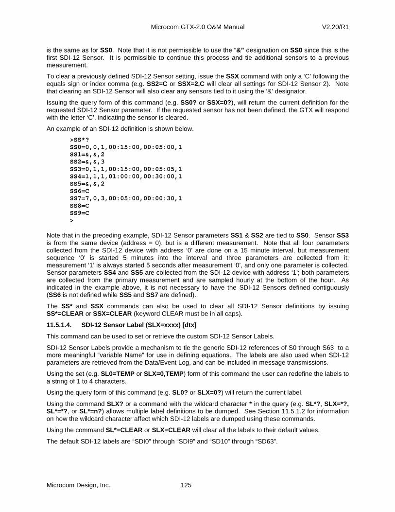
Microcom GTX-2.0 O&M Manual V2.20/R1
Microcom Design, Inc. 125
is the same as for SS0. Note that it is not permissible to use the “&” designation on SS0 since this is the first SDI-12 Sensor. It is permissible to continue this process and tie additional sensors to a previous measurement.
To clear a previously defined SDI-12 Sensor setting, issue the SSX command with only a ‘C’ following the equals sign or index comma (e.g. SS2=C or SSX=2,C will clear all settings for SDI-12 Sensor 2). Note that clearing an SDI-12 Sensor will also clear any sensors tied to it using the ‘&’ designator.
Issuing the query form of this command (e.g. SS0? or SSX=0?), will return the current definition for the requested SDI-12 Sensor parameter. If the requested sensor has not been defined, the GTX will respond with the letter ‘C’, indicating the sensor is cleared.
An example of an SDI-12 definition is shown below.
>SS*? SS0=0,0,1,00:15:00,00:05:00,1 SS1=&,&,2 SS2=&,&,3 SS3=0,1,1,00:15:00,00:05:05,1 SS4=1,1,1,01:00:00,00:30:00,1 SS5=&,&,2 SS6=C SS7=7,0,3,00:05:00,00:00:30,1 SS8=C SS9=C >
Note that in the preceding example, SDI-12 Sensor parameters SS1 & SS2 are tied to SS0. Sensor SS3 is from the same device (address = 0), but is a different measurement. Note that all four parameters collected from the SDI-12 device with address ‘0’ are done on a 15 minute interval, but measurement sequence ‘0’ is started 5 minutes into the interval and three parameters are collected from it; measurement ‘1’ is always started 5 seconds after measurement ‘0’, and only one parameter is collected. Sensor parameters SS4 and SS5 are collected from the SDI-12 device with address ‘1’; both parameters are collected from the primary measurement and are sampled hourly at the bottom of the hour. As indicated in the example above, it is not necessary to have the SDI-12 Sensors defined contiguously (SS6 is not defined while SS5 and SS7 are defined).
The SS* and SSX commands can also be used to clear all SDI-12 Sensor definitions by issuing SS*=CLEAR or SSX=CLEAR (keyword CLEAR must be in all caps).
11.5.1.4. SDI-12 Sensor Label (SLX=xxxx) [dtx]
This command can be used to set or retrieve the custom SDI-12 Sensor Labels.
SDI-12 Sensor Labels provide a mechanism to tie the generic SDI-12 references of S0 through S63 to a more meaningful “variable Name” for use in defining equations. The labels are also used when SDI-12 parameters are retrieved from the Data/Event Log, and can be included in message transmissions.
Using the set (e.g. SL0=TEMP or SLX=0,TEMP) form of this command the user can redefine the labels to a string of 1 to 4 characters.
Using the query form of this command (e.g. SL0? or SLX=0? ) will return the current label.
Using the command SLX? or a command with the wildcard character * in the query (e.g. SL*? , SLX=*?, SL*=*? , or SL*=n? ) allows multiple label definitions to be dumped. See Section 11.5.1.2 for information on how the wildcard character affect which SDI-12 labels are dumped using these commands.
Using the command SL*=CLEAR or SLX=CLEAR will clear all the labels to their default values.
The default SDI-12 labels are “SDI0” through “SDI9” and “SD10” through “SD63”.
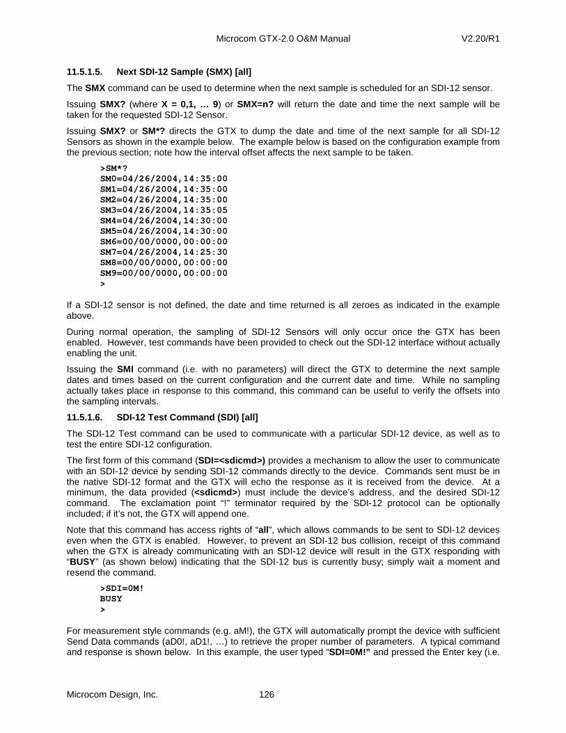
Microcom GTX-2.0 O&M Manual V2.20/R1
Microcom Design, Inc. 126
11.5.1.5. Next SDI-12 Sample (SMX) [all]
The SMX command can be used to determine when the next sample is scheduled for an SDI-12 sensor.
Issuing SMX? (where X = 0,1, … 9) or SMX=n? will return the date and time the next sample will be taken for the requested SDI-12 Sensor.
Issuing SMX? or SM*? directs the GTX to dump the date and time of the next sample for all SDI-12 Sensors as shown in the example below. The example below is based on the configuration example from the previous section; note how the interval offset affects the next sample to be taken.
>SM*? SM0=04/26/2004,14:35:00 SM1=04/26/2004,14:35:00 SM2=04/26/2004,14:35:00 SM3=04/26/2004,14:35:05 SM4=04/26/2004,14:30:00 SM5=04/26/2004,14:30:00 SM6=00/00/0000,00:00:00 SM7=04/26/2004,14:25:30 SM8=00/00/0000,00:00:00 SM9=00/00/0000,00:00:00 >
If a SDI-12 sensor is not defined, the date and time returned is all zeroes as indicated in the example above.
During normal operation, the sampling of SDI-12 Sensors will only occur once the GTX has been enabled. However, test commands have been provided to check out the SDI-12 interface without actually enabling the unit.
Issuing the SMI command (i.e. with no parameters) will direct the GTX to determine the next sample dates and times based on the current configuration and the current date and time. While no sampling actually takes place in response to this command, this command can be useful to verify the offsets into the sampling intervals.
11.5.1.6. SDI-12 Test Command (SDI) [all]
The SDI-12 Test command can be used to communicate with a particular SDI-12 device, as well as to test the entire SDI-12 configuration.
The first form of this command (SDI=<sdicmd>) provides a mechanism to allow the user to communicate with an SDI-12 device by sending SDI-12 commands directly to the device. Commands sent must be in the native SDI-12 format and the GTX will echo the response as it is received from the device. At a minimum, the data provided (<sdicmd> ) must include the device’s address, and the desired SDI-12 command. The exclamation point “!” terminator required by the SDI-12 protocol can be optionally included; if it’s not, the GTX will append one.
Note that this command has access rights of “all ”, which allows commands to be sent to SDI-12 devices even when the GTX is enabled. However, to prevent an SDI-12 bus collision, receipt of this command when the GTX is already communicating with an SDI-12 device will result in the GTX responding with “BUSY” (as shown below) indicating that the SDI-12 bus is currently busy; simply wait a moment and resend the command.
>SDI=0M! BUSY >
For measurement style commands (e.g. aM!), the GTX will automatically prompt the device with sufficient Send Data commands (aD0!, aD1!, …) to retrieve the proper number of parameters. A typical command and response is shown below. In this example, the user typed “SDI=0M!” and pressed the Enter key (i.e.
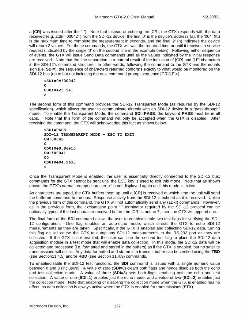
Microcom GTX-2.0 O&M Manual V2.20/R1
Microcom Design, Inc. 127
a [CR] was issued after the “!”). Note that instead of echoing the [CR], the GTX responds with the data received (e.g. atttn=‘00042’ ) from the SDI-12 device; the first ‘0’ is the device’s address (a), the ‘004’ (ttt) is the maximum time to complete the measurement in seconds, and the final ‘2’ (n) indicates the device will return 2 values. For these commands, the GTX will wait the required time or until it receives a service request (indicated by the single ‘0’ on the second line in the example below). Following either sequence of events, the GTX will issue Send Data commands until all the values indicated by the initial response are received. Note that the line separation is a natural result of the inclusion of [CR] and [LF] characters in the SDI-12’s command structure. In other words, following the command to the GTX and the equals sign (i.e. SDI=), the sequence of characters returned conforms exactly to what would be monitored on the SDI-12 bus (up to but not including the next command prompt sequence [CR][LF]>).
>SDI=0M!00042 0 0D0!0+25.9+1 >
The second form of this command provides the SDI-12 Transparent Mode (as required by the SDI-12 specification), which allows the user to communicate directly with an SDI-12 device in a “pass-through” mode. To enable the Transparent Mode, the command SDI=PASS; the keyword PASS must be in all caps. Note that this form of the command will only be accepted when the GTX is disabled. After receiving the command, the GTX will acknowledge this fact as shown below.
>SDI=PASS SDI-12 TRANSPARENT MODE - ESC TO EXIT 0M!00042 0 0D0!0+9.96+10 0M1!00041 00 0D0!0+94.9633 >
Once the Transparent Mode is enabled, the user is essentially directly connected to the SDI-12 bus; commands for the GTX cannot be sent until the ESC key is used to exit this mode. Note that as shown above, the GTX’s normal prompt character ‘>’ is not displayed again until this mode is exited.
As characters are typed, the GTX buffers them up until a [CR] is received at which time the unit will send the buffered command to the bus. Response activity from the SDI-12 is echoed as it is received. Unlike the previous form of this command, the GTX will not automatically send any {aDx!} commands. However, as in the previous form, the exclamation point “!” terminator required by the SDI-12 protocol can be optionally typed; if the last character received before the [CR] is not an ‘!’, then the GTX will append one.
The final form of the SDI command allows the user to enable/disable two test flags for verifying the SDI-12 configuration. One flag enables an auto-echo mode, which directs the GTX to echo SDI-12 measurements as they are taken. Specifically, if the GTX is enabled and collecting SDI-12 data, turning this flag on will cause the GTX to dump any SDI-12 measurements to the RS-232 port as they are collected. If the GTX is not enabled, the user can use the second test flag to place the SDI-12 data acquisition module in a test mode that will enable data collection. In this mode, the SDI-12 data will be collected and processed (i.e. formatted and stored in the buffers) as if the GTX is enabled, but no satellite transmissions will occur. Any data formatted and stored in a transmit buffer can be verified using the TBD (see Section11.4.5) and/or RBD (see Section 11.4.9) commands.
To enable/disable the SDI-12 test functions, the SDI command is issued with a single numeric value between 0 and 3 (inclusive). A value of zero (SDI=0) clears both flags and hence disables both the echo and test collection mode. A value of three (SDI=3) sets both flags, enabling both the echo and test collection. A value of one (SDI=1) enables just the echo mode, and a value of two (SDI=2) enables just the collection mode. Note that enabling or disabling the collection mode when the GTX is enabled has no affect, as data collection is always active when the GTX is enabled for transmissions (ETX).
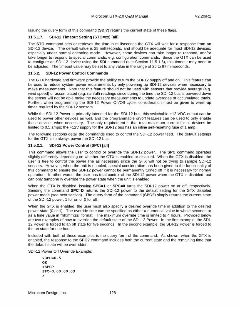
Microcom GTX-2.0 O&M Manual V2.20/R1
Microcom Design, Inc. 128
Issuing the query form of this command (SDI?) returns the current state of these flags.
11.5.1.7. SDI-12 Timeout Setting (STO=xx) [all]
The STO command sets or retrieves the time in milliseconds the GTX will wait for a response from an SDI-12 device. The default value is 25 milliseconds, and should be adequate for most SDI-12 devices, especially under normal operating mode. However, some devices can take longer to respond, and/or take longer to respond to special commands, e.g. configuration commands. Since the GTX can be used to configure an SDI-12 device using the SDI command (see Section 11.5.1.6), this timeout may need to be adjusted. The timeout value may be set to any value in the range of 25 to 87 milliseconds.
11.5.2. SDI-12 Power Control Commands
The GTX hardware and firmware provide the ability to turn the SDI-12 supply off and on. This feature can be used to reduce system power requirements by only powering up SDI-12 devices when necessary to make measurements. Note that this feature should not be used with sensors that provide average (e.g. wind speed) or accumulated (e.g. rainfall) readings since during the time the SDI-12 bus is powered down the sensor will not be able make the necessary measurements to update averages or accumulated totals. Further, when programming the SDI-12 Power On/Off cycle, consideration must be given to warm-up times required by the SDI-12 sensors.
While the SDI-12 Power is primarily intended for the SDI-12 bus, this switchable +12 VDC output can be used to power other devices as well, and the programmable on/off features can be used to only enable these devices when necessary. The only requirement is that total maximum current for all devices be limited to 0.5 amps; the +12V supply for the SDI-12 bus has an inline self-resetting fuse of 1 amp.
The following sections detail the commands used to control the SDI-12 power feed. The default settings for the GTX is to always power the SDI-12 bus.
11.5.2.1. SDI-12 Power Control (SPC) [all]
This command allows the user to control or override the SDI-12 power. The SPC command operates slightly differently depending on whether the GTX is enabled or disabled. When the GTX is disabled, the user is free to control the power line as necessary since the GTX will not be trying to sample SDI-12 sensors. However, when the unit is enabled, special consideration has been given to the functionality of this command to ensure the SDI-12 power cannot be permanently turned off if it is necessary for normal operation. In other words, the user has total control of the SDI-12 power when the GTX is disabled, but can only temporarily override the power state when the unit is enabled.
When the GTX is disabled, issuing SPC=1 or SPC=0 turns the SDI-12 power on or off, respectively. Sending the command SPC=D returns the SDI-12 power to the default setting for the GTX disabled power mode (see next section). The query form of the command (SPC?) simply returns the current state of the SDI-12 power; 1 for on or 0 for off.
When the GTX is enabled, the user must also specify a desired override time in addition to the desired power state (0 or 1). The override time can be specified as either a numerical value in whole seconds or as a time value in “hh:mm:ss” format. The maximum override time is limited to 4 hours. Provided below are two examples of how to override the default state of the SDI-12 Power. In the first example, the SDI-12 Power is forced to an off state for five seconds. In the second example, the SDI-12 Power is forced to the on state for one hour.
Included with both of these examples is the query form of the command. As shown, when the GTX is enabled, the response to the SPC? command includes both the current state and the remaining time that the default state will be overridden.
SDI-12 Power Off Override Example:
>SPC=0,5 OK >SPC? SPC=0,00:00:03 >
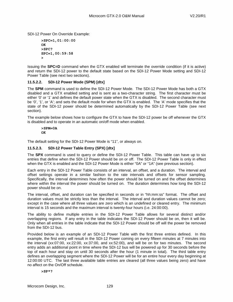
Microcom GTX-2.0 O&M Manual V2.20/R1
Microcom Design, Inc. 129
SDI-12 Power On Override Example:
>SPC=1,01:00:00 OK >SPC? SPC=1,00:59:58 >
Issuing the SPC=D command when the GTX enabled will terminate the override condition (if it is active) and return the SDI-12 power to the default state based on the SDI-12 Power Mode setting and SDI-12 Power Table (see next two sections).
11.5.2.2. SDI-12 Power Mode (SPM) [dtx]
The SPM command is used to define the SDI-12 Power Mode. The SDI-12 Power Mode has both a GTX disabled and a GTX enabled setting and is sent as a two-character string. The first character must be either ‘0’ or ‘1’ and defines the default power state when the GTX is disabled. The second character must be ‘0’, ‘1’, or ‘A’; and sets the default mode for when the GTX is enabled. The ‘A’ mode specifies that the state of the SDI-12 power should be determined automatically by the SDI-12 Power Table (see next section).
The example below shows how to configure the GTX to have the SDI-12 power be off whenever the GTX is disabled and to operate in an automatic on/off mode when enabled.
>SPM=0A OK
The default setting for the SDI-12 Power Mode is “11”, or always on.
11.5.2.3. SDI-12 Power Table Entry (SPX) [dtx]
The SPX command is used to query or define the SDI-12 Power Table. This table can have up to six entries that define when the SDI-12 Power should be on or off. The SDI-12 Power Table is only in effect when the GTX is enabled and the SDI-12 Power Mode is either “0A” or “1A” (see previous section).
Each entry in the SDI-12 Power Table consists of an interval, an offset, and a duration. The interval and offset settings operate in a similar fashion to the rate intervals and offsets for sensor sampling. Specifically, the interval determines how often the power should be turned on and the offset determines where within the interval the power should be turned on. The duration determines how long the SDI-12 power should be on.
The interval, offset, and duration can be specified in seconds or in “hh:mm:ss” format. The offset and duration values must be strictly less than the interval. The interval and duration values cannot be zero; except in the case where all three values are zero which is an undefined or cleared entry. The minimum interval is 15 seconds and the maximum interval is twenty-four hours (i.e. 24:00:00).
The ability to define multiple entries in the SDI-12 Power Table allows for several distinct and/or overlapping regions. If any entry in the table indicates the SDI-12 Power should be on, then it will be. Only when all entries in the table indicate that the SDI-12 Power should be off will the power be removed from the SDI-12 bus.
Provided below is an example of an SDI-12 Power Table with the first three entries defined. In this example, the first entry will result in the SDI-12 Power coming on every fifteen minutes at 7 minutes into the interval (xx:07:00, xx:22:00, xx:37:00, and xx:52:00), and will be on for two minutes. The second entry adds an additional point in time where the SDI-12 bus will be powered up for 30 seconds before the top of each hour and stay on until 30 seconds after the hour (1 minute in total). The third table entry defines an overlapping segment where the SDI-12 Power will be for an entire hour every day beginning at 12:00:00 UTC. The last three available table entries are cleared (all three values being zero) and have no affect on the On/Off schedule.
>SP*?

Microcom GTX-2.0 O&M Manual V2.20/R1
Microcom Design, Inc. 130
SP0=00:15:00,00:07:00,00:02:00 SP1=01:00:00,00:59:30,00:01:00 SP2=24:00:00,12:00:00,01:00:00 SP3=00:00:00,00:00:00,00:00:00 SP4=00:00:00,00:00:00,00:00:00 SP5=00:00:00,00:00:00,00:00:00 >
As the above example indicates, the command SP*? returns all six entries in the SDI-12 Power Table using a format where the table index is the last character of the command. Using the SPX? command provides the same information, but each response line will begin with “SPX=n,… ” where n is the table index.
To query an individual setting use either SPn? or SPX=n? , where n is the desired table index value.
To clear an individual table entry use either SPn=C or SPX=n,C. To clear the entire table use the command SPC=CLEAR .
11.5.3. Internal Sensor Data Collection Setup and T est Commands
The following sections detail the data collection setup and test commands implemented in the GTX for Internal Sensors. Internal Sensors include both equations and the physical internal hardware sensors; i.e. the temperature sensor, the internal tipping bucket counter, and the battery (or supply) voltage. When the Internal Sensor is defined to be a hardware sensor, the specified internal sensors will be sampled, collected, and processed by the GTX. When the Internal Sensor is defined to be an equation, the GTX will evaluate the equation and then process the resultant parameter.
As the parameters are collected, they are passed to the data format and storage module where they can be included in the Data/Event Log, the Timed transmission buffer, and/or Random transmission buffer. These parameters can also be used to trigger random reports.
To allow maximum flexibility, the configuration of the Internal Sensor data collection is independent of the data storage functions. In other words, the commands described in the following subsections only define what internal parameters are sampled and/or what equations are evaluated, what to do with the data samples once they’re collected is defined separately.
11.5.3.1. Number of Internal Sensors (ISN=xx) [dtx]
The ISN command allows the user to specify the maximum number of Internal Sensor parameters to be implemented. As explained in Section 5, the configuration memory of the GTX is soft. In other words, while the size of the memory in bytes is fixed, how the available memory is utilized can be defined by the user.
This command configures the memory allocation to reserve enough memory to provide the requested number Internal Sensor parameter definitions. If sufficient configuration memory is not available for the specified number of parameters, the GTX will respond with an error indication.
The user can specify the number of Internal Sensor parameters to be a minimum of 5 (for backward compatibility) and up to a maximum of 64 (provided sufficient memory is available). The default configuration (ConfigDefault ) allocates memory for five Internal Sensor parameters.
Before an Internal Sensor with an index higher than the currently specified number of Internal Sensor parameters can be defined, this command must be used to make the configuration memory for the desired sensor available. Using this command to reduce the number of available Internal Sensors (e.g. to make room for other soft configuration parameters), will free the associated configuration memory and delete any defined Internal Sensors above the new maximum.
11.5.3.2. Internal Sensor Command Basics
The following three sections provide information on using the ISX, ILX, and IMX commands. These commands share a common approach to referencing the specific Internal Sensor parameter. Specifically,
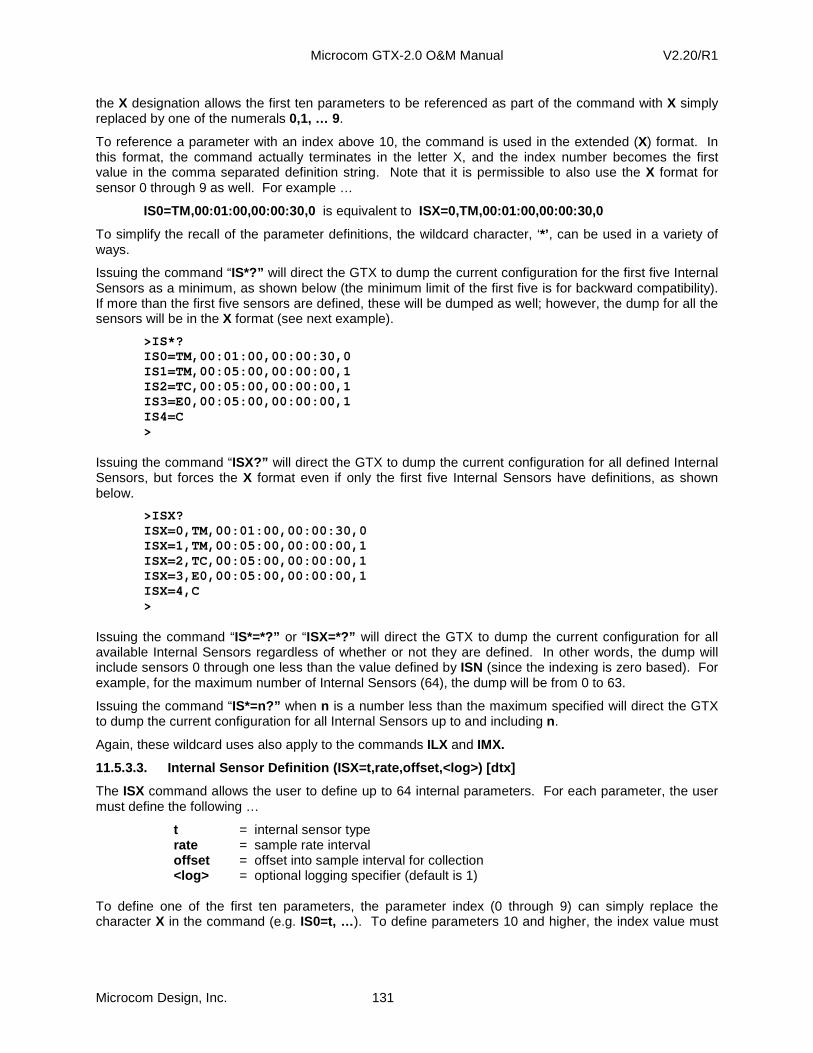
Microcom GTX-2.0 O&M Manual V2.20/R1
Microcom Design, Inc. 131
the X designation allows the first ten parameters to be referenced as part of the command with X simply replaced by one of the numerals 0,1, … 9.
To reference a parameter with an index above 10, the command is used in the extended (X) format. In this format, the command actually terminates in the letter X, and the index number becomes the first value in the comma separated definition string. Note that it is permissible to also use the X format for sensor 0 through 9 as well. For example …
IS0=TM,00:01:00,00:00:30,0 is equivalent to ISX=0,TM,00:01:00,00:00:30,0
To simplify the recall of the parameter definitions, the wildcard character, ‘*’, can be used in a variety of ways.
Issuing the command “IS*?” will direct the GTX to dump the current configuration for the first five Internal Sensors as a minimum, as shown below (the minimum limit of the first five is for backward compatibility). If more than the first five sensors are defined, these will be dumped as well; however, the dump for all the sensors will be in the X format (see next example).
>IS*? IS0=TM,00:01:00,00:00:30,0 IS1=TM,00:05:00,00:00:00,1 IS2=TC,00:05:00,00:00:00,1 IS3=E0,00:05:00,00:00:00,1 IS4=C >
Issuing the command “ISX?” will direct the GTX to dump the current configuration for all defined Internal Sensors, but forces the X format even if only the first five Internal Sensors have definitions, as shown below.
>ISX? ISX=0,TM,00:01:00,00:00:30,0 ISX=1,TM,00:05:00,00:00:00,1 ISX=2,TC,00:05:00,00:00:00,1 ISX=3,E0,00:05:00,00:00:00,1 ISX=4,C >
Issuing the command “IS*=*?” or “ISX=*?” will direct the GTX to dump the current configuration for all available Internal Sensors regardless of whether or not they are defined. In other words, the dump will include sensors 0 through one less than the value defined by ISN (since the indexing is zero based). For example, for the maximum number of Internal Sensors (64), the dump will be from 0 to 63.
Issuing the command “IS*=n?” when n is a number less than the maximum specified will direct the GTX to dump the current configuration for all Internal Sensors up to and including n.
Again, these wildcard uses also apply to the commands ILX and IMX.
11.5.3.3. Internal Sensor Definition (ISX=t,rate,of fset,<log>) [dtx]
The ISX command allows the user to define up to 64 internal parameters. For each parameter, the user must define the following …
t = internal sensor type rate = sample rate interval offset = offset into sample interval for collection <log> = optional logging specifier (default is 1)
To define one of the first ten parameters, the parameter index (0 through 9) can simply replace the character X in the command (e.g. IS0=t, …). To define parameters 10 and higher, the index value must
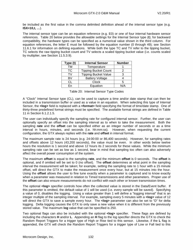
Microcom GTX-2.0 O&M Manual V2.20/R1
Microcom Design, Inc. 132
be included as the first value in the comma delimited definition ahead of the internal sensor type (e.g. ISX=10,t, …).
The internal sensor type can be an equation reference (e.g. E0) or one of four internal hardware sensor references. Table 20 below provides the allowable settings for the Internal Sensor type (t); for backward compatibility, the hardware types can be specified as a numerical value shown in the third column. For equation references, the letter E must be followed by the equation number (0 through 49); see Section 11.6.1 for information on defining equations. While both the type TC and TV refer to the tipping bucket, TC selects the raw tipping bucket count and TV selects a scaled tipping bucket value (i.e. counts scaled by multiplier, see Section 11.5.3.9).
Type (t) Internal Sensor Number TM Temperature 1 TC Tipping Bucket Count 2 TV Tipping Bucket Value 3 BV Battery Voltage 4 CL Clock 5 En Equation N/A
Table 20: Internal Sensor Type Codes A “Clock” Internal Sensor type (CL), can be used to capture a time and/or date stamp that can then be included in a transmission buffer or used as a value in an equation. When selecting this type of Internal Sensor, the <log> field is replaced with a <format> field specifying the format of time/date stamp. One of thirty-three predefined format strings must be specified. The available format strings are defined in Table 11 in Section 6.1.2.1.5.
The user can individually specify the sampling rate for configured internal sensor. Further, the user can optionally specify an offset into the sampling interval as to when to take the measurement. Both the sampling rate and the offset can be specified either as an integer number of seconds or as a time interval in hours, minutes, and seconds (i.e. hh:mm:ss). However, when requesting the current configuration, the GTX always replies with the rate and offset in interval format.
The maximum sample rate is 24 hours (e.g. 24:00:00 or 86,400 seconds). However, for sampling rates and offsets above 12 hours (43,200 seconds), the value must be even. In other words below twelve hours the resolution is 1 second and above 12 hours its 2 seconds for these values. While the minimum sampling rate can be set as low as 1 second, bear in mind that sampling too often can also adversely affect the overall power consumption of the system.
The maximum offset is equal to the sampling rate , and the minimum offset is 0 seconds. The offset is optional, and if omitted will be set to 0 (no offset). The offset determines at what point in the sampling interval the measurement will be taken; for example, setting the sampling rate to 1 hour with a 15 minute offset, will direct the GTX to make the measurement once every hour, but at 15 minutes into the hour. Using the offset allows the user to fine tune exactly when a parameter is captured and to know exactly when a parameter was measured in relation to Timed transmissions and other parameters. Proper use of the offset can also ensure measurements do not conflict with each other or known transmission times.
The optional <log> specifier controls how often the collected value is stored in the Data/Event buffer. If this parameter is omitted, the default value of 1 will be used (i.e. every sample will be saved). Specifying a value of 0, disables the logging. Using a value greater than 1 will define a “logging interval” that is an integer multiple of the sampling interval. For example, sampling every 5 minutes with a <log> value of 12 will direct the GTX to save a sample every hour. The <log> parameter can also be set to “D” for delta logging. Delta logging causes the GTX to only save a new value when it is different from the previously stored value. The maximum log value that can be specified is 250.
Two optional flags can also be included with the optional <log> specifier. These flags are defined by including the characters H and/or L. Appending an H flag to the log specifier directs the GTX to check the Random Report Triggers for a trigger type of High or Rise tied to this sensor. Likewise, if the L flag is appended, the GTX will check the Random Report Triggers for a trigger type of Low or Fall tied to this

Microcom GTX-2.0 O&M Manual V2.20/R1
Microcom Design, Inc. 133
sensor. If such a Random Trigger exists, and the value is such that it is above (for H) or below (for L) the trigger limit the value will always be logged. This allows data to be logged less frequently, i.e. only when conditions warrant.
To clear a previously defined Internal Sensor setting, this command must be issued with only a ‘C’ as the definition string (e.g. IS2=C or ISX=2,C will clear all settings for Internal Sensor 2).
Issuing the query form of this command (e.g. IS0? or ISX=0?), will return the current definition for the requested Internal Sensor. If the requested sensor has not been defined, the GTX will respond with the letter ‘C’, indicating the sensor is cleared.
An example of Internal Sensor definition shown below.
>IS*? IS0=TM,00:01:00,00:00:30,0 IS1=TM,00:05:00,00:00:00,1 IS2=TC,00:05:00,00:00:00,1 IS3=E0,00:05:00,00:00:00,1 IS4=CL,00:05:00,00:00:00,J:H:M:S >
Note that in the preceding example, Internal Sensor parameters IS0 & IS1 are both sampling the internal temperature sensor. However, IS0 samples the temperature on a one-minute interval, while IS1 samples the temperature on a five-minute interval. Further, note that IS0 is sampled at the bottom of the minute (i.e. the offset is 00:00:30), while IS1 is sampled at the top of the minute (albeit only every 5 minutes). Internal Sensor 2 is sampling the Tipping Bucket Count and IS3 will execute equation E0 every 5 minutes. Internal Sensor IS4 is specified to be a Clock (CL) sensor that will capture the current Julian day, hour, minute, and second fields.
The IS* and ISX commands can also be used to clear all Internal Sensor definitions by issuing IS*=CLEAR or ISX=CLEAR (keyword CLEAR must be in all caps).
11.5.3.4. Internal Sensor Label (ILX=xxxx) [dtx]
This command can be used to set or retrieve the custom Internal Sensor Labels.
Internal Sensor Labels provide a mechanism to tie the generic references of I0 through I63 to a more meaningful “variable Name” for use in defining equations. The labels are also used when Internal Sensor parameters are retrieved from the Data/Event Log, and can be included in message transmissions.
Using the set (e.g. IL0=TEMP or ILX=0,TEMP) form of this command, the user can redefine the labels to any string of 1 to 4 characters.
Using the query form of this command (e.g. IL0? or ILX=0? ) will return the current label.
Using the command ILX? or a command with the wildcard character, ‘*’, in the query (e.g. IL*? , ILX=*?, IL*=*? , or IL*=n? ) allows multiple label definitions to be dumped. See Section 11.5.3.2 for information on how the wildcard character affects which Internal Sensor labels are dumped using these commands.
Using the command IL*=CLEAR or ILX=CLEAR will clear all the labels to their default values.
The default Internal Sensor labels are “INT0” through “INT9” and “IN10” through “IN63”.
11.5.3.5. Next Internal Sensor Sample (IMX) [all]
The IMX command can be used to determine when the next sample is scheduled for an internal data sensor.
Issuing IMX? (where X = 0,1, … 9) or IMX=n? will return the date and time the next sample will be taken for the requested sensor.
Issuing IMX? or IM*? will direct the GTX to dump the date and time of the next sample for all Internal Sensors as shown in the example below. The example below is based on the configuration example from the previous section; note how the interval offset affects the next sample to be taken.
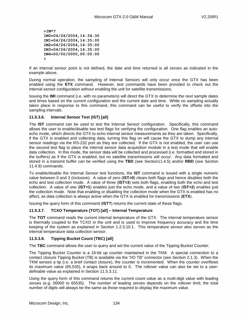
Microcom GTX-2.0 O&M Manual V2.20/R1
Microcom Design, Inc. 134
>IM*? IM0=04/26/2004,14:34:30 IM1=04/26/2004,14:35:00 IM2=04/26/2004,14:35:00 IM3=04/26/2004,14:35:00 IM4=00/00/0000,00:00:00 >
If an internal sensor point is not defined, the date and time returned is all zeroes as indicated in the example above.
During normal operation, the sampling of Internal Sensors will only occur once the GTX has been enabled using the ETX command. However, test commands have been provided to check out the internal sensor configuration without enabling the unit for satellite transmissions.
Issuing the IMI command (i.e. with no parameters) will direct the GTX to determine the next sample dates and times based on the current configuration and the current date and time. While no sampling actually takes place in response to this command, this command can be useful to verify the offsets into the sampling intervals.
11.5.3.6. Internal Sensor Test (IST) [all]
The IST command can be used to test the Internal Sensor configuration. Specifically, this command allows the user to enable/disable two test flags for verifying the configuration. One flag enables an auto-echo mode, which directs the GTX to echo internal sensor measurements as they are taken. Specifically, if the GTX is enabled and collecting data, turning this flag on will cause the GTX to dump any internal sensor readings via the RS-232 port as they are collected. If the GTX is not enabled, the user can use the second test flag to place the internal sensor data acquisition module in a test mode that will enable data collection. In this mode, the sensor data will be collected and processed (i.e. formatted and stored in the buffers) as if the GTX is enabled, but no satellite transmissions will occur. Any data formatted and stored in a transmit buffer can be verified using the TBD (see Section11.4.5) and/or RBD (see Section 11.4.9) commands.
To enable/disable the Internal Sensor test functions, the IST command is issued with a single numeric value between 0 and 3 (inclusive). A value of zero (IST=0) clears both flags and hence disables both the echo and test collection mode. A value of three (IST=3) sets both flags, enabling both the echo and test collection. A value of one (IST=1) enables just the echo mode, and a value of two (IST=2) enables just the collection mode. Note that enabling or disabling the collection mode when the GTX is enabled has no affect, as data collection is always active when the GTX is enabled for transmissions (ETX).
Issuing the query form of this command (IST?) returns the current state of these flags.
11.5.3.7. TCXO Temperature (TOT) [all] – Internal T emperature
The TOT command reads the current internal temperature of the GTX. The internal temperature sensor is thermally coupled to the TCXO in the unit and is used to improve frequency accuracy and the time keeping of the system as explained in Section 1.2.3.10.1. This temperature sensor also serves as the internal temperature data collection sensor.
11.5.3.8. Tipping Bucket Count (TBC) [all]
The TBC command allows the user to query and set the current value of the Tipping Bucket Counter.
The Tipping Bucket Counter is a 16-bit up counter maintained in the TKM. A special connection to a contact closure Tipping Bucket (TB) is available via the “I/O TB” connector (see Section 2.1.3). When the TKM senses a tip (i.e. a brief contact closure), the counter is incremented. When the counter overflows its maximum value (65,535), it wraps back around to 0. The rollover value can also be set to a user-definable value as explained in Section 11.5.3.11.
Using the query form of this command returns the current count value as a multi-digit value with leading zeroes (e.g. 00000 to 65535). The number of leading zeroes depends on the rollover limit; the total number of digits will always be the same as those required to display the maximum value.
Microcom GTX-2.0 O&M Manual V2.20/R1
Microcom Design, Inc. 135
Using the set form of the command, the TB count can be initialized to any value or cleared back to 0; use of leading zeroes when setting the count is optional.
11.5.3.9. Tipping Bucket Value (TBV) [all]
The TBV command allows the user to query scaled value of the Tipping Bucket Counter. The scaled value is equal to the counts (TBC) times the Tipping Bucket Multiplier (TBM).
The format of the Tipping Bucket Value depends on both the rollover limit (TBR) and the scaling multiplier (TBM). The number of decimal places (digits to the right of the decimal point) will be the same as the multiplier. The number of digits to the left of the decimal point is determined by computing the maximum value with leading zeroes as necessary. For example, if the rollover count is set to 4000 with a multiplier of 0.25, the maximum reading is 999.75 (0.25*(4000-1)). Accordingly, for this example, the value will be between 000.00 and 999.75, inclusive.
11.5.3.10. Tipping Bucket Multiplier (TBM=xxx) [dtx ]
The TBM command allows the user to set or query the scaling multiplier for the Tipping Bucket Value. The scaled value is equal to the counts (TBC) times the Tipping Bucket Multiplier (TBM).
The Multiplier can be set to one of twelve values: 0.01, 0.02, 0.025, 0.05, 0.1, 0.2, 0.25, 0.5, 1, 2, 2.5, or 5. The default value is 1.
11.5.3.11. Tipping Bucket Rollover (TBR=xxxxx) [dtx ]
The TBR command allows the user to set or query the Tipping Bucket Rollover setting. The Rollover parameters determines the maximum counts the Tipping Bucket Counter can reach before wrapping around to 0; i.e. one less than the rollover value. Setting this parameter to 0 allows the count to reached its maximum 16-bit value of 65535.
The default value is 0.
11.5.3.12. Tipping Bucket Auto Clear (TBA=xxx) [dtx ]
The TBA command is used to enable the Tipping Bucket Auto Clear function. This function allows the Tipping Bucket Counter to be automatically cleared to 0 at a predefined interval. The interval can be a fixed number of days (xxx = 1 to 120), or one of five special modes (D ⇒ daily, M ⇒ monthly, Q ⇒ quarterly, B ⇒ bi-annually, and A ⇒ annually). Setting TBA=0 disables the Auto Clear function; the TB Counter will count to its maximum and wrap around to 0.
When specifying the daily reset option, the command must also include a two-digit value (00 to 23) the determines at what hour in the day the reset will occur. For example, TBA=D,00 specifies that the tipping bucket count should be zeroed at the top of the UTC day. Specifying a different hour can be used to cause the daily reset to occur at the beginning of each day based on local time.
For a fixed number of days interval, the GTX will down count a counter at midnight of each day and clear the TB count when the day counter reaches zero; after which, the day counter is reset to the programmed value. When setting this mode, an optional initial day count value may also be provided separated from the interval by a comma. For example, to get the count to be reset once a week on Sunday at 00:00:00 (i.e. just after midnight Saturday) when placing the unit into service on Friday, the command TBA=7,2 would be used. If an initial count is not provided, then the day counter will be initialized to the interval.
For the special modes, the Tipping Bucket Counter will only be reset when a month rollover occurs at midnight (i.e. time changes from 23:59:59 to 00:00:00). The four modes select which month(s) the reset occurs. Setting the mode to Monthly will cause the counter to be reset at the beginning of each month. For Quarterly mode, the counter is only reset when the new month is January, April, July, or October. Bi-annually selects a reset only on January 1 and July 1, and Annually only reset the counter once a year on the 1ST of January.
The query form of the command returns the current setting (0, day interval, or special mode).
Issuing the TBA command without any parameters or the question mark in the day interval mode will return the interval and the current value of the day counter (i.e. the number of days until the next clear).
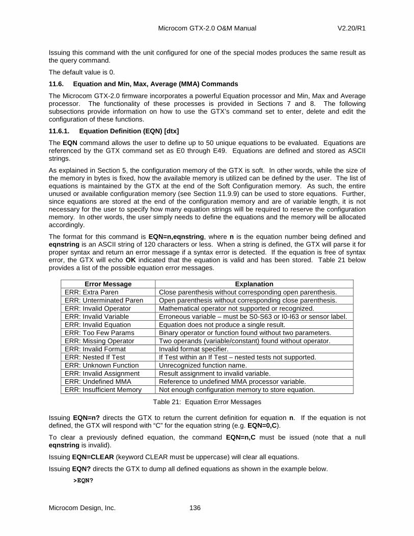
Microcom GTX-2.0 O&M Manual V2.20/R1
Microcom Design, Inc. 136
Issuing this command with the unit configured for one of the special modes produces the same result as the query command.
The default value is 0.
11.6. Equation and Min, Max, Average (MMA) Commands
The Microcom GTX-2.0 firmware incorporates a powerful Equation processor and Min, Max and Average processor. The functionality of these processes is provided in Sections 7 and 8. The following subsections provide information on how to use the GTX’s command set to enter, delete and edit the configuration of these functions.
11.6.1. Equation Definition (EQN) [dtx]
The EQN command allows the user to define up to 50 unique equations to be evaluated. Equations are referenced by the GTX command set as E0 through E49. Equations are defined and stored as ASCII strings.
As explained in Section 5, the configuration memory of the GTX is soft. In other words, while the size of the memory in bytes is fixed, how the available memory is utilized can be defined by the user. The list of equations is maintained by the GTX at the end of the Soft Configuration memory. As such, the entire unused or available configuration memory (see Section 11.9.9) can be used to store equations. Further, since equations are stored at the end of the configuration memory and are of variable length, it is not necessary for the user to specify how many equation strings will be required to reserve the configuration memory. In other words, the user simply needs to define the equations and the memory will be allocated accordingly.
The format for this command is EQN=n,eqnstring , where n is the equation number being defined and eqnstring is an ASCII string of 120 characters or less. When a string is defined, the GTX will parse it for proper syntax and return an error message if a syntax error is detected. If the equation is free of syntax error, the GTX will echo OK indicated that the equation is valid and has been stored. Table 21 below provides a list of the possible equation error messages.
Error Message Explanation ERR: Extra Paren Close parenthesis without corresponding open parenthesis. ERR: Unterminated Paren Open parenthesis without corresponding close parenthesis. ERR: Invalid Operator Mathematical operator not supported or recognized. ERR: Invalid Variable Erroneous variable – must be S0-S63 or I0-I63 or sensor label. ERR: Invalid Equation Equation does not produce a single result. ERR: Too Few Params Binary operator or function found without two parameters. ERR: Missing Operator Two operands (variable/constant) found without operator. ERR: Invalid Format Invalid format specifier. ERR: Nested If Test If Test within an If Test – nested tests not supported. ERR: Unknown Function Unrecognized function name. ERR: Invalid Assignment Result assignment to invalid variable. ERR: Undefined MMA Reference to undefined MMA processor variable. ERR: Insufficient Memory Not enough configuration memory to store equation.
Table 21: Equation Error Messages
Issuing EQN=n? directs the GTX to return the current definition for equation n. If the equation is not defined, the GTX will respond with “C” for the equation string (e.g. EQN=0,C).
To clear a previously defined equation, the command EQN=n,C must be issued (note that a null eqnstring is invalid).
Issuing EQN=CLEAR (keyword CLEAR must be uppercase) will clear all equations.
Issuing EQN? directs the GTX to dump all defined equations as shown in the example below.
>EQN?
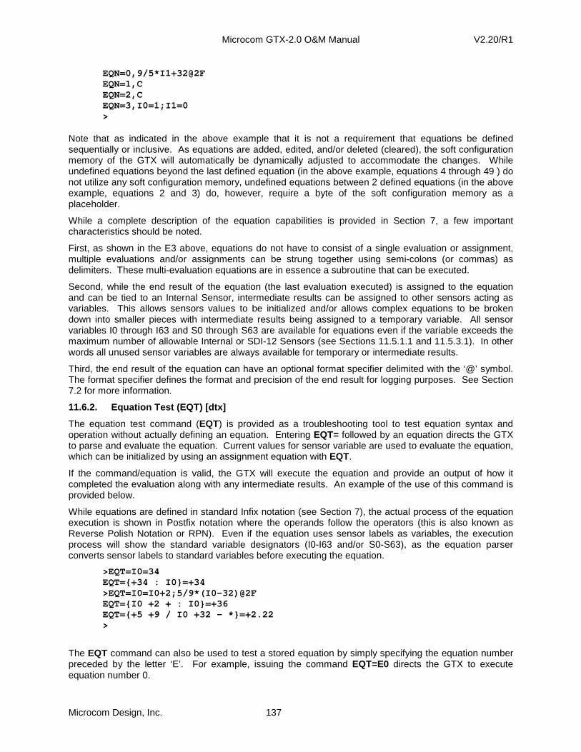
Microcom GTX-2.0 O&M Manual V2.20/R1
Microcom Design, Inc. 137
EQN=0,9/5*I1+32@2F EQN=1,C EQN=2,C EQN=3,I0=1;I1=0 >
Note that as indicated in the above example that it is not a requirement that equations be defined sequentially or inclusive. As equations are added, edited, and/or deleted (cleared), the soft configuration memory of the GTX will automatically be dynamically adjusted to accommodate the changes. While undefined equations beyond the last defined equation (in the above example, equations 4 through 49 ) do not utilize any soft configuration memory, undefined equations between 2 defined equations (in the above example, equations 2 and 3) do, however, require a byte of the soft configuration memory as a placeholder.
While a complete description of the equation capabilities is provided in Section 7, a few important characteristics should be noted.
First, as shown in the E3 above, equations do not have to consist of a single evaluation or assignment, multiple evaluations and/or assignments can be strung together using semi-colons (or commas) as delimiters. These multi-evaluation equations are in essence a subroutine that can be executed.
Second, while the end result of the equation (the last evaluation executed) is assigned to the equation and can be tied to an Internal Sensor, intermediate results can be assigned to other sensors acting as variables. This allows sensors values to be initialized and/or allows complex equations to be broken down into smaller pieces with intermediate results being assigned to a temporary variable. All sensor variables I0 through I63 and S0 through S63 are available for equations even if the variable exceeds the maximum number of allowable Internal or SDI-12 Sensors (see Sections 11.5.1.1 and 11.5.3.1). In other words all unused sensor variables are always available for temporary or intermediate results.
Third, the end result of the equation can have an optional format specifier delimited with the ‘@’ symbol. The format specifier defines the format and precision of the end result for logging purposes. See Section 7.2 for more information.
11.6.2. Equation Test (EQT) [dtx]
The equation test command (EQT) is provided as a troubleshooting tool to test equation syntax and operation without actually defining an equation. Entering EQT= followed by an equation directs the GTX to parse and evaluate the equation. Current values for sensor variable are used to evaluate the equation, which can be initialized by using an assignment equation with EQT.
If the command/equation is valid, the GTX will execute the equation and provide an output of how it completed the evaluation along with any intermediate results. An example of the use of this command is provided below.
While equations are defined in standard Infix notation (see Section 7), the actual process of the equation execution is shown in Postfix notation where the operands follow the operators (this is also known as Reverse Polish Notation or RPN). Even if the equation uses sensor labels as variables, the execution process will show the standard variable designators (I0-I63 and/or S0-S63), as the equation parser converts sensor labels to standard variables before executing the equation.
>EQT=I0=34 EQT={+34 : I0}=+34 >EQT=I0=I0+2;5/9*(I0-32)@2F EQT={I0 +2 + : I0}=+36 EQT={+5 +9 / I0 +32 - *}=+2.22 >
The EQT command can also be used to test a stored equation by simply specifying the equation number preceded by the letter ‘E’. For example, issuing the command EQT=E0 directs the GTX to execute equation number 0.
Microcom GTX-2.0 O&M Manual V2.20/R1
Microcom Design, Inc. 138
11.6.3. Equation Constants
The GTX-2.0 supports up to 64 user definable equation constants that can be modified even when the GTX is enabled. Equations can be defined with one or more user configurable constants, and the commands defined in this section may be used to specify the values for these constants. Moreover, unlike the equations themselves which can only be modified when the GTX is disabled, equation constants can changed while the GTX is enabled for operation.
As explained in more detail in Section 7.1.2.2, this feature provides a mechanism to allow for calibration of a sensor without the need to disable the GTX to make changes or corrections to the calibration values. For example, assume it is desirable or necessary to be able to provide a scaling and offset correction to SDI-12 sensor 0. While the user can define an equation to apply the necessary calibration factors directly in an equation (e.g. “0.95*S0 + 0.10”), changing the factors requires changing the equation which also requires disabling the GTX. However, if the calibration equation is defined as “K0*S0+K1”, then the calibration factors can be changed without having to disable the GTX.
11.6.3.1. Number of Equation Constants (EKN=xx) [dt x]
The EKN command allows the user to specify the maximum number of Equation Constants to be implemented. As explained in Section 5, the configuration memory of the GTX is soft. In other words, while the size of the memory in bytes is fixed, how the available memory is utilized can be defined by the user.
This command configures the memory allocation to reserve enough memory to provide the requested number of Equation Constants and their corresponding labels. If sufficient configuration memory is not available for the specified number of parameters, the GTX will respond with an error indication.
The user allocate no Equation Constants or up to a maximum of 64 (provided sufficient memory is available). The default configuration (ConfigDefault ) allocates no memory for contants.
Before an Equation Constant with an index higher than the currently specified number of constants can be defined, this command must be used to expand the number of constant. Using this command to reduce the number of available constants (e.g. to make room for other soft configuration parameters), will free the associated configuration memory and delete any defined Equation Constants above the new maximum. Note that while the constant values can be changed while the GTX is enabled, the number of constants can not.
11.6.3.2. Equation Constant Value (EKV) [all]
The EKV command allows the user to define the actual value for an Equation Constant.
The basic format for the EKV command is shown below:
EKV=n,val where,
n = constant number (0-63) val = the constant’s value
To query the current value of a specific constant, the command EKV=n? is used, where the desired constant number is ‘n’. The default value for a constant is zero, i.e. until it is explicitly defined by the user all constants are initially set to 0.
Issuing the command EKV? or EKV=*? , will direct the GTX to dump all defined constants, i.e. up to the maximum number as specified by the EKN command.
Another unique feature of Equation Constants are that any changes to their values can be captured in the Data/Event log. When the GTX is enabled, constant changes are always logged. By default, setting a constant when the GTX is disabled will not log the value. However, the user can override this default and force the value to be logged by appending a comma and the letter ‘L ’ after the val (value) field, e.g. EKV=0,1.23,L will set K0=1.23 and log the new value. Note that logging constants when the GTX is disabled also requires that the internal clock be set.

Microcom GTX-2.0 O&M Manual V2.20/R1
Microcom Design, Inc. 139
11.6.3.3. Equation Constant Label (EKL) [dtx]
Like SDI-12 and Internal Sensors, Equation Constants have a default designation of K0 through K63. However, also like sensors, these constants can have a descriptive name or label attached to them to improve the readability of an equation. The EKL command can be used to set or retrieve the custom Equation Constant Labels.
Using the set (e.g. EKL=0,SCL & EKL=1,OFS ) form of this command, the user can redefine the labels to any string of 1 to 4 characters.
Using the query form of this command (e.g. EKL=0? ) will return the current label for the constant.
Using the query command with the wildcard character, ‘*’, in the query (i.e. EKL=*? ) allows all label definitions to be dumped.
Using the command EKL=CLEAR will clear all the labels to their default values. The default Equation Constant labels are “KNS0” through “KNS9” and “KN10” through “KN63”.
11.6.4. Equation Variable (EQV) [all]
The equation variable command (EQV) allows a simple mechanism to query the current value of one of the standard equation variables, i.e. I0-I63 and S0-S63. Entering EQV= followed by the desired variable will return the current numeric value for that variable.
Note that this operation could also be accomplished using the EQT command with just the desired variable as the equation. However, this actually causes the test equation to be parsed and executed, which could interfere with an operational equation when the GTX is enabled. Accordingly, the EQT has an access level of “dtx” to prevent this conflict. As such, the EQV command, with an access level of “all ” must be used to query variables when the GTX is enabled.
The EQV command simply returns the stored value of the variable so it doesn’t require equation execution and does not pose a potential conflict.
11.6.5. Number of Min, Max, Average Processors (MMN =xx) [dtx]
The MMN command allows the user to specify the maximum number of MMA Processors to be implemented. As explained in Section 5, the configuration memory of the GTX is soft. In other words, while the size of the memory in bytes is fixed, how the available memory is utilized can be defined by the user.
This command configures the memory allocation to reserve enough memory to provide the requested number MMA Processor definitions. If sufficient configuration memory is not available for the requested processors, the GTX will respond with an error indication.
The user can specify the number of MMA Processors to be a minimum of 1 and up to a maximum of 64 (provided sufficient memory is available). The default configuration (ConfigDefault ) does not allocate any memory for MMA processing, i.e. effectively it sets MMN=0.
Before an MMA Processor with an index higher than the currently allocated number of MMA Processors can be defined, this command must be used to make the configuration memory for the desired processor available. Using this command to reduce the number of available MMA Processors (e.g. to make room for other soft configuration parameters), will free the associated configuration memory and delete any defined MMA Processors above the new maximum.
11.6.6. Min, Max, Average Definition (MMA=sensor,ra te,offset,<flags>) [dtx]
The MMA command allows the user to define up to 64 MMA Processors. For each processor, the user must define the following …
sensor = Internal or SDI-12 Sensor rate = processing rate interval offset = offset into processing interval for collection <flags> = optional logging and vector average flags; N X G or V (default is none)

Microcom GTX-2.0 O&M Manual V2.20/R1
Microcom Design, Inc. 140
When defining an MMA Processor, the first field provided in the MMA must be the index number of the MMA Processor. For example, MMA=0,I0,01:00:00,00:00:01,NXG ties MMA Processor 0 to Internal Sensor 0.
The sensor type can be either an Internal or SDI-12 sensor; note that since Internal Sensors can also be tied to an equation (see Section 11.5.3.3), an MMA Processor can also operate on an equation. While it is possible to define complex equations that operate on one or more parameters and produce minimum, maximum, and average results, the MMA Processor greatly simplifies this process for a single sensor parameter.
As a sensor is sampled, the value of the sensor is automatically passed to the MMA processing routines. If an MMA Processor is tied to this sensor, then the minimum and maximums will be updated accordingly (along with a time stamp for the value). Next, the value will be added to an accumulator and a count value will be incremented. At the processing rate , the GTX will extract and process the cumulative information (i.e. the average will be calculated), forward it to the Data/Event logger and the transmit buffers, and then reset the accumulation values for the next interval.
The user can individually specify the accumulation rate for configured Processor. Further, the user can optionally specify an offset into the accumulation interval as to when to the Min, Max, and Average values will be acquired and processed. Both the processing rate and the offset can be specified either as an integer number of seconds or as a time interval in hours, minutes, and seconds (i.e. hh:mm:ss). However, when requesting the current configuration, the GTX always replies with the rate and offset in interval format.
The maximum processing rate is 24 hours (e.g. 24:00:00 or 86,400 seconds). However, for processing rates and offsets above 12 hours (43,200 seconds), the value must be even. In other words below twelve hours the resolution is 1 second and above 12 hours its 2 seconds for these values. While the minimum processing rate can be set as low as 10 seconds, bear in mind that sampling too often can also adversely affect the overall power consumption of the system. Note that the processing rate for an MMA Processor is independent of the sampling interval for the sensor.
The maximum offset is equal to the processing rate , and the minimum offset is 0 seconds. The offset is optional, and if omitted will be set to 0 (no offset). The offset determines at what point in the processing interval the MMA data will be processed; for example, setting the processing rate to 1 hour with a 15 minute offset, will direct the GTX to make the process the MMA data once every hour, but at 15 minutes into the hour. Using the offset allows the user to fine tune exactly when the processing is performed and to know exactly when the average was computed in relation to Timed transmissions and other parameters. Proper use of the offset can also ensure measurements do not conflict with each other or known transmission times.
The optional <flags> specifier can be used to direct the MMA results to be stored in the Data/Event buffer. If this parameter is omitted, then no MMA results will be logged; however, they can still be included in the satellite transmission buffers (see Section 11.7.3.3). The flags are the single letters ‘N’, ‘X’, and ‘G’ (i.e. the last letter of the abbreviations for miN, maX, and avG). The flags can be provided in any combination and in any order. However, when logging or storing in a transmission buffer, the results will always be included in the order of Min, Max, and Average; un-flagged results will simply not be stored.
The optional <flags> specifier is also used to configure the MMA processor to perform a unity gain vector average instead of the standard numerical average. Including the letter ‘V’ (in addition to any logging letters) will direct this MMA processor to operate in vector average mode.
To clear a previously defined MMA Processor definition, the MMA command must be issued with only the comma delimited index number and the letter ‘C’ as the definition string (e.g. MMA=2,C will clear MMA Processor 2).
Issuing the query form of this command (e.g. MMA=n? ), will return the current definition for the requested MMA Processor. If the requested processor has not been defined, the GTX will respond with the letter ‘C’.
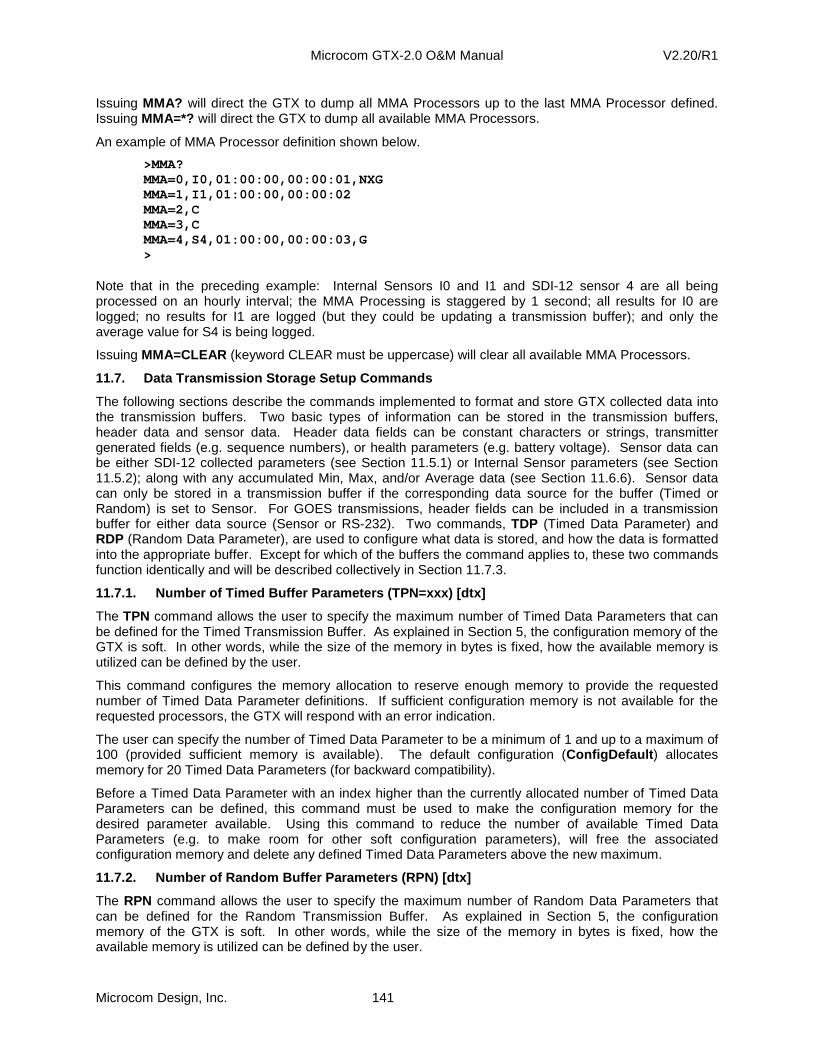
Microcom GTX-2.0 O&M Manual V2.20/R1
Microcom Design, Inc. 141
Issuing MMA? will direct the GTX to dump all MMA Processors up to the last MMA Processor defined. Issuing MMA=*? will direct the GTX to dump all available MMA Processors.
An example of MMA Processor definition shown below.
>MMA? MMA=0,I0,01:00:00,00:00:01,NXG MMA=1,I1,01:00:00,00:00:02 MMA=2,C MMA=3,C MMA=4,S4,01:00:00,00:00:03,G >
Note that in the preceding example: Internal Sensors I0 and I1 and SDI-12 sensor 4 are all being processed on an hourly interval; the MMA Processing is staggered by 1 second; all results for I0 are logged; no results for I1 are logged (but they could be updating a transmission buffer); and only the average value for S4 is being logged.
Issuing MMA=CLEAR (keyword CLEAR must be uppercase) will clear all available MMA Processors.
11.7. Data Transmission Storage Setup Commands
The following sections describe the commands implemented to format and store GTX collected data into the transmission buffers. Two basic types of information can be stored in the transmission buffers, header data and sensor data. Header data fields can be constant characters or strings, transmitter generated fields (e.g. sequence numbers), or health parameters (e.g. battery voltage). Sensor data can be either SDI-12 collected parameters (see Section 11.5.1) or Internal Sensor parameters (see Section 11.5.2); along with any accumulated Min, Max, and/or Average data (see Section 11.6.6). Sensor data can only be stored in a transmission buffer if the corresponding data source for the buffer (Timed or Random) is set to Sensor. For GOES transmissions, header fields can be included in a transmission buffer for either data source (Sensor or RS-232). Two commands, TDP (Timed Data Parameter) and RDP (Random Data Parameter), are used to configure what data is stored, and how the data is formatted into the appropriate buffer. Except for which of the buffers the command applies to, these two commands function identically and will be described collectively in Section 11.7.3.
11.7.1. Number of Timed Buffer Parameters (TPN=xxx) [dtx]
The TPN command allows the user to specify the maximum number of Timed Data Parameters that can be defined for the Timed Transmission Buffer. As explained in Section 5, the configuration memory of the GTX is soft. In other words, while the size of the memory in bytes is fixed, how the available memory is utilized can be defined by the user.
This command configures the memory allocation to reserve enough memory to provide the requested number of Timed Data Parameter definitions. If sufficient configuration memory is not available for the requested processors, the GTX will respond with an error indication.
The user can specify the number of Timed Data Parameter to be a minimum of 1 and up to a maximum of 100 (provided sufficient memory is available). The default configuration (ConfigDefault ) allocates memory for 20 Timed Data Parameters (for backward compatibility).
Before a Timed Data Parameter with an index higher than the currently allocated number of Timed Data Parameters can be defined, this command must be used to make the configuration memory for the desired parameter available. Using this command to reduce the number of available Timed Data Parameters (e.g. to make room for other soft configuration parameters), will free the associated configuration memory and delete any defined Timed Data Parameters above the new maximum.
11.7.2. Number of Random Buffer Parameters (RPN) [d tx]
The RPN command allows the user to specify the maximum number of Random Data Parameters that can be defined for the Random Transmission Buffer. As explained in Section 5, the configuration memory of the GTX is soft. In other words, while the size of the memory in bytes is fixed, how the available memory is utilized can be defined by the user.
Microcom GTX-2.0 O&M Manual V2.20/R1
Microcom Design, Inc. 142
This command configures the memory allocation to reserve enough memory to provide the requested number of Random Data Parameter definitions. If sufficient configuration memory is not available for the requested processors, the GTX will respond with an error indication.
The user can specify the number of Random Data Parameter to be a minimum of 1 and up to a maximum of 40 (provided sufficient memory is available). The default configuration (ConfigDefault ) allocates memory for 20 Random Data Parameters (for backward compatibility).
Before a Random Data Parameter with an index higher than the currently allocated number of Random Data Parameters can be defined, this command must be used to make the configuration memory for the desired parameter available. Using this command to reduce the number of available Random Data Parameters (e.g. to make room for other soft configuration parameters), will free the associated configuration memory and delete any defined Random Data Parameters above the new maximum.
11.7.3. Timed and Random Data Parameter Definition (TDP & RDP) [dtx]
The TDP and RDP commands are used to configure which data parameters are loaded into the Timed and Random transmit buffers, respectively. Since these two commands have identical usage, they are described in this section collectively; for the remainder of this section, the command XDP will be used to indicate both TDP and RDP.
In addition to determining what data is loaded into the appropriate buffer, the XDP command also determines the format of the data loaded. For either transmit buffer, the maximum number of parameters that may be defined is determined by the associated TPN or RPN commands (see previous two sections). While the nomenclature indicates that Header parameters should appear first, this is not actually a requirement; parameters (header or sensor) may be defined to be loaded into the buffer in any order. However, when the data source is RS-232, only Header parameters may be defined, and in this case, they will always be transmitted prior to sending the RS-232 loaded data.
The basic format for the XDP command is XDP=pn,id,pcnt<pflags>,fw_res,flags,scale,offset . However, depending on the parameter id and/or the data format selected for the buffer (ASCII, Pseudo, or Binary), not all parameters are required nor allowed. Provided below is the definition of the configuration fields for the XDP command.
pn = parameter number id = parameter identifier or designator (e.g. H0, S0, I0, etc.) pcnt = parameter count - number of measurements to store <pflags> = parameter flags – allows Min, Max, and Average data to be appended fw_res = field width or resolution for each parameter measurement flags = parameter flags scale = binary conversion scale offset = binary conversion offset
The parameter number (pn ) is used to designate the order in which the parameters appear in the transmit buffer; pn=0 is the first parameter, pn=1 is next and so on. When querying a specific data point, a special version of the query command is required. Specifically, to request the current configuration for a data parameter, the parameter number must be given after an equal sign and then be followed by a question mark. The command XDP=0? directs the transmitter to return the current configuration for parameter 0 (i.e. pn=0 ).
Since pn determines the order parameters appear in the buffer, parameters must be contiguous. Having a null parameter embedded in a sequence of parameters will prevent subsequent parameters from being included in the buffer. For example, if parameter 0 and parameter 2 are defined but parameter 1 is not, only parameter 0 will be loaded into the buffer. However, it is not necessary to define the parameters sequentially; parameter 2 may be defined before either parameter 0 or 1.
To facilitate editing the order of parameters, special versions of the XDP command have been implemented to allow clearing, insertion, and deletion of parameters. Specifically, …
XDP=pnC will clear parameter pn , but will not change the order of the remaining parameters
Microcom GTX-2.0 O&M Manual V2.20/R1
Microcom Design, Inc. 143
XDP=pnD will delete parameter pn , and will drop all subsequent parameters down by one XDP=pnI will insert a null (undefined) parameter at location pn , and move all subsequent
parameters up by one Note that for all three of these special formats, the operation letter (C, D, or I – can be either upper or lower case) must immediately follow the parameter number (pn ).
Note that when using the insert operation, a null or undefined parameter is inserted, which must be later defined to restore the contiguous nature of the parameter definition. In addition, if the last parameter (e.g. 19 in the default configuration) is defined when an insert operation is performed, its definition will be replaced with the preceding parameter (e.g. 18) and the previous definition will be irretrievably lost. To prevent losing parameters, use TPN or RPN to increase the maximum number of parameters before the insertion operation.
To clear the entire parameter definition for a transmit buffer, the command XDP=CLEAR (keyword CLEAR must be in all caps) is used.
Issuing the command XDP? will direct the transmitter to dump all defined parameters up to, but not including the first null parameter. If no parameters are defined (or the first parameter is null), the response will be XDP=0C. To dump all parameters regardless of whether or not they are defined, the command XDP=*? must be issued. Any parameter with a null definition will have the response format XDP=pnC .
Following the parameter number field, the next field identifies the parameter type (id ). There are three types of parameter ids that may be specified; Header parameters (Hn), SDI-12 Sensor parameters (Sn), and Internal Sensor parameters (In); note that since an Internal Sensor can be tied to an equation, equation results can also be included. In addition to the parameter type designator (H, S, or I), the user must specify the parameter id number, n. For header parameters, the id number determines the specific type of header parameter. For SDI-12 and internal sensor parameters, the id number correlates to an SDI-12 (Section 11.5.1.1) or Internal (Section 11.5.3.1) sensor collection definition. Additional information with regard to Header and Sensor parameters is provided in Sections 11.7.3.1 and 11.7.3.2, respectively.
For Sensor parameters, the next field that must be defined is the parameter count (pcnt ), which is the number of historical parameters to save and transmit. For example, if an SDI-12 sensor is sampled once every ten minutes and it is desired to have the last hour’s worth of sample transmitted, then the parameter count (pcnt ) would be set to 6. The order in which the parameters are stored and transmitted is determined by either the Timed Data Order or the Random Data Order; the data order can be oldest to newest or newest to oldest.
For Sensor parameters, three optional flags (pflags ) can be included immediately (i.e. without a comma) following the parameter count (pcnt ). These optional flags determine which, if any, MMA results are stored in the transmission buffer following the historical parameter values. If this parameter is omitted, then no MMA results will be included. The flags are the single letters ‘N’, ‘X’, and ‘G’ (i.e. the last letter of the abbreviations for miN, maX, and avG). The flags can be provided in any combination and in any order. However, when they are stored in the transmission buffer, the results will always be included in the order of Min, Max, and Average; un-flagged results will simply not be included. Note that it is also possible to only include the MMA values for this parameter by using a pcnt of 0; otherwise, zero is not permissible value for the parameter count.
Following the parameter count, Sensor parameters must also have a field width defined for ASCII data format, or a resolution for defined binary or pseudo-binary formats. For ASCII formatted data, the field width determines the number of characters (1-16) to be reserved for each parameter in the list. For binary formatted data, the resolution is the number of bits (1-24) to reserve, save and transmit for each parameter. For pseudo-binary formatted data, the resolution is in pseudo-binary characters (1, 2, 3, or 4), which correlates to multiples of 6 bits (N=6, 12, 18, or 24).
For binary and pseudo-binary data, the resolution can be either positive or negative. Positive resolutions indicate that the binary representation of the value is unsigned, while a negative resolution indicates the binary value is in signed two’s complement format. In addition to determining the number of binary bits (N) to use to represent the transmitted parameter, the resolution also determines the maximum (positive
Microcom GTX-2.0 O&M Manual V2.20/R1
Microcom Design, Inc. 144
⇒ 2N-1, negative ⇒ 2N-1-1) and minimum (positive ⇒ 0, negative ⇒ -2N-1) limits. After conversion to binary, the parameter is ranged check and clamped to these limits.
For ASCII formatted data, if the number of characters in the parameter exceeds the field width the parameter string is truncated from the right to fit the field width. If the number of characters is less than the field width, the parameter string is padded with spaces from the left to fill the field width (i.e. right justified).
While the parameter count (pcnt ) and field width/resolution (fw_res ) are required for sensor parameters, there are not permitted for header parameters. Header parameters have predefined internal settings for these fields.
Following the fw_res field, the user may specify optional formatting flags for the parameter. Formatting flags are single ASCII characters that further define how the parameter is formatted in the transmit buffer. While not all formatting flags are applicable to all parameter types and/or data formats (ASCII, binary, or pseudo-binary), provided below is a summary of the available formatting flags.
S = Include a space separator after parameter list R = Include [CR] separator after parameter list N = Include [LF] separator after parameter list L = Include Label field before parameter list with a colon after label LB = Include Label field before parameter list with a colon before label LX = Include Label field before parameter list without a colon Z = Include leading zeroes on parameter values (ASCII only) C = Parameter is a counter value – allow binary wrap
Multiple flag characters are stringed together without commas or spaces. For example, to include a carriage return and a line feed after a parameter list, the flag field would be defined as either RN or NR. Note that the format flags can be specified in any order; regardless of the flag sequence in the definition, separator characters are appended in the order shown in the list above (i.e. space, [CR], [LF]). The label flag (L) is applicable to both Header (e.g. battery volts under load, forward power, reflected power, etc.) and Sensor parameters (i.e. SDI-12 and Internal). The count flag (C) is only applicable to sensor parameters, and only when in binary or pseudo-binary format; this flag allows count style parameters (e.g. tipping bucket count) to be sent with reduced resolution by removing the maximum limit restriction. Specifically, instead of clamping the binary value to a maximum, the value is allowed to wrap around zero.
When the data format for the corresponding transmit buffer is either pseudo-binary or binary, then the transmitter requires scale and offset conversion values to convert the numeric (i.e. ASCII decimal) parameter value to binary. As with the parameter count and resolution fields, these values are predetermined and cannot be entered for Header parameters. If the user does not explicitly specify these values for a sensor parameter, then the scale is set to 1 and the offset is set to 0. Prior to formatting and loading a binary or pseudo-binary parameter, the decimal value is converted to binary using the equation below. After conversion, the value is range checked and, if necessary, limited as explained previously.
binary = scale * (decimal – offset ) (decimal to binary conversion) While the parameter count, field width, scale, and offset values for Header parameters cannot be configured by the user, they can be read by issuing the XDP command without any parameters. Using the command in this format also validates the parameter list; and if valid, will initialize the appropriate buffer. Following a valid initialization, the transmitter will dump the parameter list similar to using the XDP? command. However, as part of this dump, the Header fields that are not user definable will be reported. If the transmitter detects an invalid parameter, then instead of dumping the parameter list, it will respond with XDP=INV,pn indicating at which parameter number the error was detected. Note that while parameter definitions are checked for validity upon entry, changing other configuration parameters could invalidate a parameter definition. For example, only Header parameters may be included with a transmission when the data source is RS-232; as such, if sensor parameters were defined with the data

Microcom GTX-2.0 O&M Manual V2.20/R1
Microcom Design, Inc. 145
source set to Sensor and then the source is changed to RS-232, then these parameter definitions will be invalid.
It should be noted that for ASCII and Pseudo-Binary formats, the data that is stored into a transmit buffer does NOT include the parity bit. Instead, the parity bit is set to odd parity just prior to transmission. This allows the data in the buffer to be dumped for verification using the terminal interface without having to deal with parity.
The following subsections provide additional specifics about transmit buffer parameter definitions with regard to Header and sensor parameters.
11.7.3.1. Header Data Parameters
As noted in the previous section, when defining a Header transmit parameter, only the parameter designator (id ) and flags are required or permitted. The remaining parameter fields are predefined by the transmitter. Provided below is a table detailing the available Header parameters and their predefined fields. Note that all Header parameters have a parameter count of 1, i.e. no historical buffering is performed.
Header parameters H0-H2 are user-definable string/character constants that will be sent identically on every transmission. These parameters are not allowed in binary format. Header parameter H0, is a platform identification string (see Section 11.7.3.1.1), and as such has a variable field width. When the transmit buffer is initialized, the field width is set to the length of the currently defined PIS string. Header parameters H1 and H2, are individually definable Pseudo-Binary (PB) characters (‘?’ to ‘~’).
H3 is a sequence counter parameter that can be used to identify missed messages. Separate sequence counters are provided for both timed and random transmissions. In ASCII format the sequence number is a value between 001 and 999. In Pseudo-Binary format, the sequence number is encoded as two PB characters; as such, the value will act as a 12-bit counter with a range of 1 to 4095. In Binary format, the sequence number is encoded as a single byte, and the value will be between 0x01 and 0xFF (1 to 255).
Header parameters H4 through H7 are measured during the carrier portion of the transmission, and included in the transmit buffer for the next message, i.e. delayed by one transmission time. The battery voltage is measured under load and recorded to a 0.1 volt resolution; note that for Pseudo-Binary format the battery voltage is encoded as a single PB character. The forward and reflected powers are in dBW to a 0.1 dB resolution. All four of these parameters may have an optional label preceding the value in ASCII format only; in the default labeling mode, these labels are the single ASCII character defined in Table 22 followed by a colon followed by a space. By specifying the appropriate flag, the colon can be moved to before the character or can be omitted entirely.
ID
Name
Param Count
Fw/Res A, P, B
Scale
Offset
Label
Related Command
H0 Platform Id String 1 V, V, E N/A N/A N/A PIS H1 Pseudo-Bin Char 1 1 1, 1, E N/A N/A N/A PB1 H2 Pseudo-Bin Char 2 1 1, 1, E N/A N/A N/A PB2 H3 Sequence Number 1 3, 2, 8 N/A N/A N/A None H4 Transmit Battery Volts 1 5, 1, 6 10.0 -9.0 B None H5 Forward Power 1 5, -2, -10 10.0 0.0 F None H6 Reflected Power 1 5, -2, -10 10.0 0.0 R None H7 Transmit Temperature 1 6, -2, -11 10.0 0.0 T None H8 GPS Latitude 1 10,4,N/A 1.0 0.0 Lat None H9 GPS Longitude 1 10,4,N/A 1.0 0.0 Lng None
Table 22: Transmit Buffer Header Parameters (V = Variable, E = Error, N/A = Not Applicable)
Header parameters H8 and H9 allow the platforms GPS location information to be included in the message. Note that except for mobile platforms, these header parameters are primarily intended for test and demonstration purposes, as this information should not typically vary from transmission to
Microcom GTX-2.0 O&M Manual V2.20/R1
Microcom Design, Inc. 146
transmission. Both of these parameters can have an optional label included ahead of the data. The position information is reported in degrees, minutes, and seconds format. Latitude degrees are positive for North and negative for South; longitude degrees are positive for East and negative for West. When the format is ASCII, a 10-character string provides this information; degrees, minutes, and seconds are separated with spaces. For pseudo-binary format, the data is reported using four characters; the first two characters are the signed degrees; the third and forth characters represent the minutes and seconds, respectively, as a single unsigned pseudo-binary character (0 to 59 = @ to {).
Note that when defining a Header parameter, the unused fields are completely omitted; do not include extraneous commas with null data for these fields. For example, to define the first parameter to be the platform id string with a [CR] and [LF] appended, the command is XDP=0,H0,RN.
Unlike sensor parameters, Header parameters may be included in a transmission even when the data source is RS-232. In this configuration, the header data is always sent ahead of any data loaded into the buffer via the serial port. Also, whenever the GTX reports a transmit buffer size configured for a data source of RS-232 with Header parameters defined, the byte counts for the Header portion and the received data portion are separated by a plus sign (e.g. 24+50). This allows the user or a host terminal to distinguish between how many bytes to be transmitted are from the header and how many are from the data.
11.7.3.1.1. Platform Identification String (PIS) [d tx]
The Platform Identification String is a user definable header parameter that may be used as constant preamble for DCP identification. The PIS is Header parameter H0 and can be up to 40 ASCII characters in length.
To clear the id string send the command PIS=. , i.e. the command plus a single period.
The default value is a null string, i.e. no characters.
11.7.3.1.2. Pseudo Binary Character 1 and 2 (PB1 an d PB2) [dtx]
PB1 and PB2 are user definable header parameters consisting of a single Pseudo-Binary character (‘?’ through ‘~’) that may be used as constant preambles. The use and definition of these values is completely up to the end user. PB1 correlates to Header parameter H1, and PB2 correlates to Header parameter H2.
These two parameters cannot be cleared, and their default values are both ‘@’.
11.7.3.2. Sensor Data Parameters
Two types of sensor data parameters may be included in a transmit buffer, SDI-12 sensor data or Internal sensor data (temperature or tipping bucket counter). For SDI-12 sensor parameters, the parameter designator (id ) is S0 through S63. For internal sensors, the parameter designator is I0 through I63. Note that in either case, the index of the parameter designator must be strictly less than the maximum number of sensors allocated for the type of sensor. The sensor does not have to necessarily be defined, but the configuration memory must support its definition. As detailed in subsequent sections, the collection rate for each sensor parameter is independently configurable. The total time spanned by the historical data in a transmit buffer for a particular parameter is a function of both the sampling rate and the parameter count (pcnt ).
When a parameter is collected, the parameter value and parameter designator are forwarded to the transmit buffer format module. The transmit buffer format module searches both the TDP and the RDP lists to determine if and where the parameter is to be inserted into the appropriate transmit buffer. After searching the two transmit parameter lists, the Random Report Trigger (RRT - see Section 11.7.4) list is also searched to determine if the parameter is to be checked against a threshold limit for triggering random reports. Note that this approach provides the flexibility to include any parameter in either transmit buffer as well as to be used to trigger random reports.
The native format for both types of sensor data is ASCII. In other words, the data passed to the transmit buffer format module is an ASCII string; e.g. the string value captured directly from an SDI-12 sensor. When the data format is ASCII, the received string is simply copied into the buffer after the older data is

Microcom GTX-2.0 O&M Manual V2.20/R1
Microcom Design, Inc. 147
shifted in the buffer to accommodate the new value (the oldest value is irretrievably lost). If the field width is less than the parameter string length, the string is truncated from the right. If the field width is greater than the string length, then the field is padded with spaces from the left (i.e. the parameter is right-justified in the buffer). Provided below is an example of a Timed Buffer Dump (TBD) with three timed parameters defined.
>TBD TBD=69 MICROCOM GTX-2.0 TIMED BUFFER 25.25 25.50 25.75 00002 00001 00000 >
The TDP definition for this example is provided below. The first timed parameter is the platform id string (PIS=MICROCOM GTX-2.0 TIMED BUFFER) followed a [CR][LF]. The second parameter is internal sensor 0, which has been configured for temperature, followed by a [CR][LF]. The last parameter is internal sensor 1, which is configured for the tipping bucket counter; no carriage or line feed is appended to this parameter list. Note that for the 2ND and 3RD parameters, three values are stored and both parameters were defined with a field width of 6 characters. Accordingly, since all the values are 5 characters, a space character is inserted before the parameter value.
>TDP? TDP=0,H0,RN TDP=1,I0,3,6,RN TDP=2,I1,3,6 >
If the data format for transmission is Pseudo-Binary, then the value is first converted to a binary representation and then encoded into Pseudo-Binary. Provided below is an example of a Random Buffer Dump (RBD) with random transmissions configured for Pseudo-Binary.
>RBD RBD=17 Acg]gvhO@@B@@A@@@ >
The RDP definition for this example is provided below. The first random parameter is PB1=A , and the second is PB2=c ; note that the use and interpretation of these characters is entirely up to the user. The third parameter is internal sensor 0, which has been configured for temperature. The last parameter is internal sensor 1, which is configured for the tipping bucket counter. While it is permissible to use parameter list separator flags (i.e. R, N, or S) in Pseudo-Binary format, typically this is not done; otherwise, the message will not achieve the maximum efficiency Pseudo-Binary can provide. Note that for the 3RD and 4TH parameters, three values are stored. However, while both use an offset of 0.0, the temperature scale is 100 and the tipping bucker scale is 1. In addition, for temperature the resolution is –2, indicating that both positive and negative (two’s complement) binary values are permitted; while the tipping bucket resolution is 3, indicating that only positive values are used. Further, the tipping bucket parameter is defined with the counter option flag (C); while not necessary for this example since 3 PB characters (i.e. 18-bits) are utilized, its inclusion does not affect operation and provides an indication of the type of parameter. However, if it’s acceptable to reduce the reported resolution of the counter to 12-bits, then only two PB characters would be required and the counter designation would be necessary.
>RDP? RDP=0,H1 RDP=1,H2 RDP=2,I0,3,-2,,100,0 RDP=3,I1,3,3,C,1,0 >
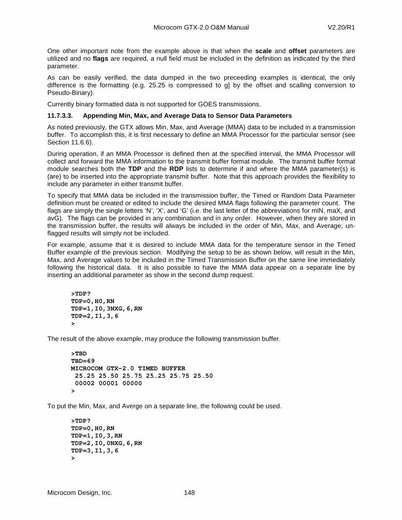
Microcom GTX-2.0 O&M Manual V2.20/R1
Microcom Design, Inc. 148
One other important note from the example above is that when the scale and offset parameters are utilized and no flags are required, a null field must be included in the definition as indicated by the third parameter.
As can be easily verified, the data dumped in the two preceeding examples is identical, the only difference is the formatting (e.g. 25.25 is compressed to g] by the offset and scalling conversion to Pseudo-Binary).
Currently binary formatted data is not supported for GOES transmissions.
11.7.3.3. Appending Min, Max, and Average Data to S ensor Data Parameters
As noted previously, the GTX allows Min, Max, and Average (MMA) data to be included in a transmission buffer. To accomplish this, it is first necessary to define an MMA Processor for the particular sensor (see Section 11.6.6).
During operation, if an MMA Processor is defined then at the specified interval, the MMA Processor will collect and forward the MMA information to the transmit buffer format module. The transmit buffer format module searches both the TDP and the RDP lists to determine if and where the MMA parameter(s) is (are) to be inserted into the appropriate transmit buffer. Note that this approach provides the flexibility to include any parameter in either transmit buffer.
To specify that MMA data be included in the transmission buffer, the Timed or Random Data Parameter definition must be created or edited to include the desired MMA flags following the parameter count. The flags are simply the single letters ‘N’, ‘X’, and ‘G’ (i.e. the last letter of the abbreviations for miN, maX, and avG). The flags can be provided in any combination and in any order. However, when they are stored in the transmission buffer, the results will always be included in the order of Min, Max, and Average; un-flagged results will simply not be included.
For example, assume that it is desired to include MMA data for the temperature sensor in the Timed Buffer example of the previous section. Modifying the setup to be as shown below, will result in the Min, Max, and Average values to be included in the Timed Transmission Buffer on the same line immediately following the historical data. It is also possible to have the MMA data appear on a separate line by inserting an additional parameter as show in the second dump request.
>TDP? TDP=0,H0,RN TDP=1,I0,3NXG,6,RN TDP=2,I1,3,6 >
The result of the above example, may produce the following transmission buffer.
>TBD TBD=69 MICROCOM GTX-2.0 TIMED BUFFER 25.25 25.50 25.75 25.25 25.75 25.50 00002 00001 00000 >
To put the Min, Max, and Averge on a separate line, the following could be used.
>TDP? TDP=0,H0,RN TDP=1,I0,3,RN TDP=2,I0,0NXG,6,RN TDP=3,I1,3,6 >

Microcom GTX-2.0 O&M Manual V2.20/R1
Microcom Design, Inc. 149
The result of the above example, may produce the following transmission buffer.
>TBD TBD=69 MICROCOM GTX-2.0 TIMED BUFFER 25.25 25.50 25.75 25.25 25.75 25.50 00002 00001 00000 >
11.7.3.4. Text Field Parameters
Fixed text strings can be included in a transmit buffers by specifying id in the TDP or RDP to be “T”. Up to a ten character string can then be defined for the parameter. In this form of the TDP or RDP command, the text string replaces the parameter count (pcnt ) field and the only other allowed field is the optional parameter flags (<pflags>) .
The example below shows how to set the TDP parameter 6 to the string “Testing123”. In this example, no optional flags are specified.
>TDP=6,T,”Testing123” The string for the Text should be enclosed in double quotes. However, when defining the text parameter, quotes can be omitted as long as the string does not include any embedded commas. In response to a query, the GTX will always enclose the text string in double quote.
Text field transmission parameters can also be defined with the optional terminator flags of S (space), C (carriage return), and L (linefeed). Also, specifying the L or LB flags designates this string as a label and will direct to GTX to include a colon either after or before, respectively, the string. The example below shows how to designate the same string as in the previous example to be a “label” string. Figure 68 in Section 9.8 shows how this text would appear in the transmit buffer.
>TDP=6,T,”Testing123”,L
11.7.4. Number of Random Triggers (RTN) [dtx]
The RTN command allows the user to specify the maximum number of Random Triggers that can be defined for Random Transmissions. As explained in Section 5, the configuration memory of the GTX is soft. In other words, while the size of the memory in bytes is fixed, how the available memory is utilized can be defined by the user.
This command configures the memory allocation to reserve enough memory to provide the requested number of Random Triggers. If sufficient configuration memory is not available for the requested processors, the GTX will respond with an error indication.
The user can specify the number of Random Triggers to be a minimum of 1 and up to a maximum of 30 (provided sufficient memory is available). The default configuration (ConfigDefault ) allocates memory for 15 Random Triggers (for backward compatibility).
Before a Random Trigger with an index higher than the currently allocated number of Random Triggers can be defined, this command must be used to make the configuration memory for the desired trigger available. Using this command to reduce the number of available Random Triggers (e.g. to make room for other soft configuration parameters), will free the associated configuration memory and delete any defined Random Triggers above the new maximum.
11.7.5. Random Report Trigger Definition (RRT) [dtx ]
In addition to being able to capture and store sensor parameters, the sensor parameters are also used to trigger Random Reports when the Random data source is configured for Sensor. Note that the sensor parameter(s) used to trigger the random report sequence does not actually have to be captured in the Random Transmit buffer.
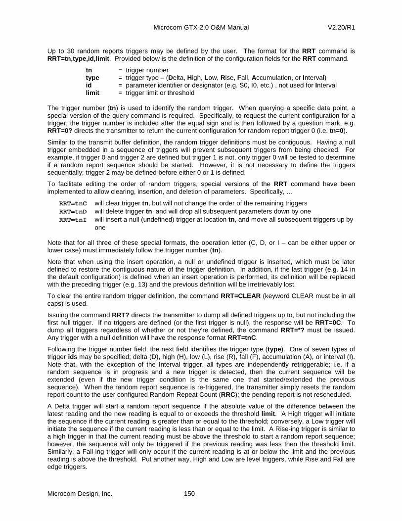
Microcom GTX-2.0 O&M Manual V2.20/R1
Microcom Design, Inc. 150
Up to 30 random reports triggers may be defined by the user. The format for the RRT command is RRT=tn,type,id,limit . Provided below is the definition of the configuration fields for the RRT command.
tn = trigger number type = trigger type – (Delta, High, Low, Rise, Fall, Accumulation, or Interval) id = parameter identifier or designator (e.g. S0, I0, etc.) , not used for Interval limit = trigger limit or threshold
The trigger number (tn ) is used to identify the random trigger. When querying a specific data point, a special version of the query command is required. Specifically, to request the current configuration for a trigger, the trigger number is included after the equal sign and is then followed by a question mark, e.g. RRT=0? directs the transmitter to return the current configuration for random report trigger 0 (i.e. tn=0 ).
Similar to the transmit buffer definition, the random trigger definitions must be contiguous. Having a null trigger embedded in a sequence of triggers will prevent subsequent triggers from being checked. For example, if trigger 0 and trigger 2 are defined but trigger 1 is not, only trigger 0 will be tested to determine if a random report sequence should be started. However, it is not necessary to define the triggers sequentially; trigger 2 may be defined before either 0 or 1 is defined.
To facilitate editing the order of random triggers, special versions of the RRT command have been implemented to allow clearing, insertion, and deletion of parameters. Specifically, …
RRT=tnC will clear trigger tn , but will not change the order of the remaining triggers RRT=tnD will delete trigger tn , and will drop all subsequent parameters down by one RRT=tnI will insert a null (undefined) trigger at location tn , and move all subsequent triggers up by
one Note that for all three of these special formats, the operation letter (C, D, or I – can be either upper or lower case) must immediately follow the trigger number (tn ).
Note that when using the insert operation, a null or undefined trigger is inserted, which must be later defined to restore the contiguous nature of the trigger definition. In addition, if the last trigger (e.g. 14 in the default configuration) is defined when an insert operation is performed, its definition will be replaced with the preceding trigger (e.g. 13) and the previous definition will be irretrievably lost.
To clear the entire random trigger definition, the command RRT=CLEAR (keyword CLEAR must be in all caps) is used.
Issuing the command RRT? directs the transmitter to dump all defined triggers up to, but not including the first null trigger. If no triggers are defined (or the first trigger is null), the response will be RRT=0C. To dump all triggers regardless of whether or not they’re defined, the command RRT=*? must be issued. Any trigger with a null definition will have the response format RRT=tnC .
Following the trigger number field, the next field identifies the trigger type (type ). One of seven types of trigger ids may be specified; delta (D), high (H), low (L), rise (R), fall (F), accumulation (A), or interval (I). Note that, with the exception of the Interval trigger, all types are independently retriggerable; i.e. if a random sequence is in progress and a new trigger is detected, then the current sequence will be extended (even if the new trigger condition is the same one that started/extended the previous sequence). When the random report sequence is re-triggered, the transmitter simply resets the random report count to the user configured Random Repeat Count (RRC); the pending report is not rescheduled.
A Delta trigger will start a random report sequence if the absolute value of the difference between the latest reading and the new reading is equal to or exceeds the threshold limit . A High trigger will initiate the sequence if the current reading is greater than or equal to the threshold; conversely, a Low trigger will initiate the sequence if the current reading is less than or equal to the limit. A Rise-ing trigger is similar to a high trigger in that the current reading must be above the threshold to start a random report sequence; however, the sequence will only be triggered if the previous reading was less then the threshold limit. Similarly, a Fall-ing trigger will only occur if the current reading is at or below the limit and the previous reading is above the threshold. Put another way, High and Low are level triggers, while Rise and Fall are edge triggers.
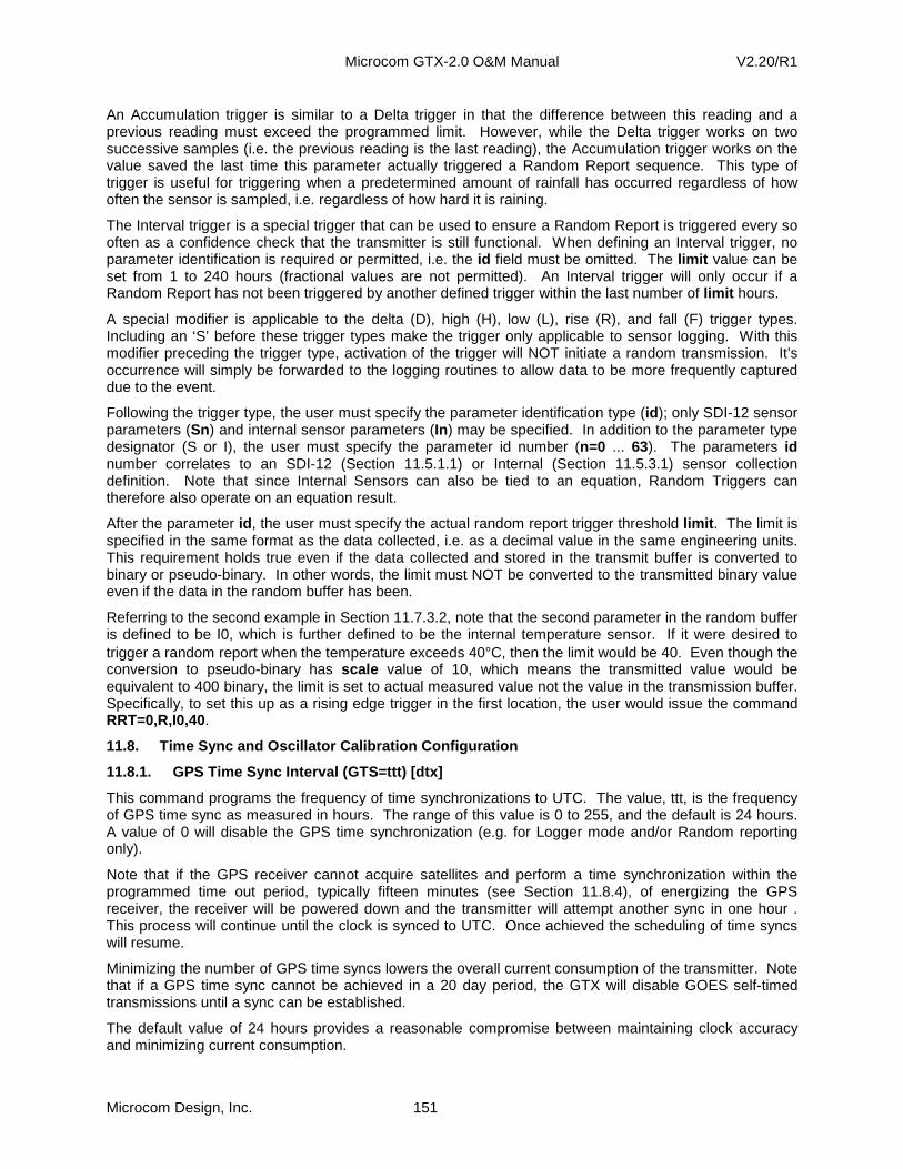
Microcom GTX-2.0 O&M Manual V2.20/R1
Microcom Design, Inc. 151
An Accumulation trigger is similar to a Delta trigger in that the difference between this reading and a previous reading must exceed the programmed limit. However, while the Delta trigger works on two successive samples (i.e. the previous reading is the last reading), the Accumulation trigger works on the value saved the last time this parameter actually triggered a Random Report sequence. This type of trigger is useful for triggering when a predetermined amount of rainfall has occurred regardless of how often the sensor is sampled, i.e. regardless of how hard it is raining.
The Interval trigger is a special trigger that can be used to ensure a Random Report is triggered every so often as a confidence check that the transmitter is still functional. When defining an Interval trigger, no parameter identification is required or permitted, i.e. the id field must be omitted. The limit value can be set from 1 to 240 hours (fractional values are not permitted). An Interval trigger will only occur if a Random Report has not been triggered by another defined trigger within the last number of limit hours.
A special modifier is applicable to the delta (D), high (H), low (L), rise (R), and fall (F) trigger types. Including an ‘S’ before these trigger types make the trigger only applicable to sensor logging. With this modifier preceding the trigger type, activation of the trigger will NOT initiate a random transmission. It’s occurrence will simply be forwarded to the logging routines to allow data to be more frequently captured due to the event.
Following the trigger type, the user must specify the parameter identification type (id ); only SDI-12 sensor parameters (Sn) and internal sensor parameters (In) may be specified. In addition to the parameter type designator (S or I), the user must specify the parameter id number (n=0 ... 63). The parameters id number correlates to an SDI-12 (Section 11.5.1.1) or Internal (Section 11.5.3.1) sensor collection definition. Note that since Internal Sensors can also be tied to an equation, Random Triggers can therefore also operate on an equation result.
After the parameter id , the user must specify the actual random report trigger threshold limit . The limit is specified in the same format as the data collected, i.e. as a decimal value in the same engineering units. This requirement holds true even if the data collected and stored in the transmit buffer is converted to binary or pseudo-binary. In other words, the limit must NOT be converted to the transmitted binary value even if the data in the random buffer has been.
Referring to the second example in Section 11.7.3.2, note that the second parameter in the random buffer is defined to be I0, which is further defined to be the internal temperature sensor. If it were desired to trigger a random report when the temperature exceeds 40°C, then the limit would be 40. Even though the conversion to pseudo-binary has scale value of 10, which means the transmitted value would be equivalent to 400 binary, the limit is set to actual measured value not the value in the transmission buffer. Specifically, to set this up as a rising edge trigger in the first location, the user would issue the command RRT=0,R,I0,40.
11.8. Time Sync and Oscillator Calibration Configur ation
11.8.1. GPS Time Sync Interval (GTS=ttt) [dtx]
This command programs the frequency of time synchronizations to UTC. The value, ttt, is the frequency of GPS time sync as measured in hours. The range of this value is 0 to 255, and the default is 24 hours. A value of 0 will disable the GPS time synchronization (e.g. for Logger mode and/or Random reporting only).
Note that if the GPS receiver cannot acquire satellites and perform a time synchronization within the programmed time out period, typically fifteen minutes (see Section 11.8.4), of energizing the GPS receiver, the receiver will be powered down and the transmitter will attempt another sync in one hour . This process will continue until the clock is synced to UTC. Once achieved the scheduling of time syncs will resume.
Minimizing the number of GPS time syncs lowers the overall current consumption of the transmitter. Note that if a GPS time sync cannot be achieved in a 20 day period, the GTX will disable GOES self-timed transmissions until a sync can be established.
The default value of 24 hours provides a reasonable compromise between maintaining clock accuracy and minimizing current consumption.
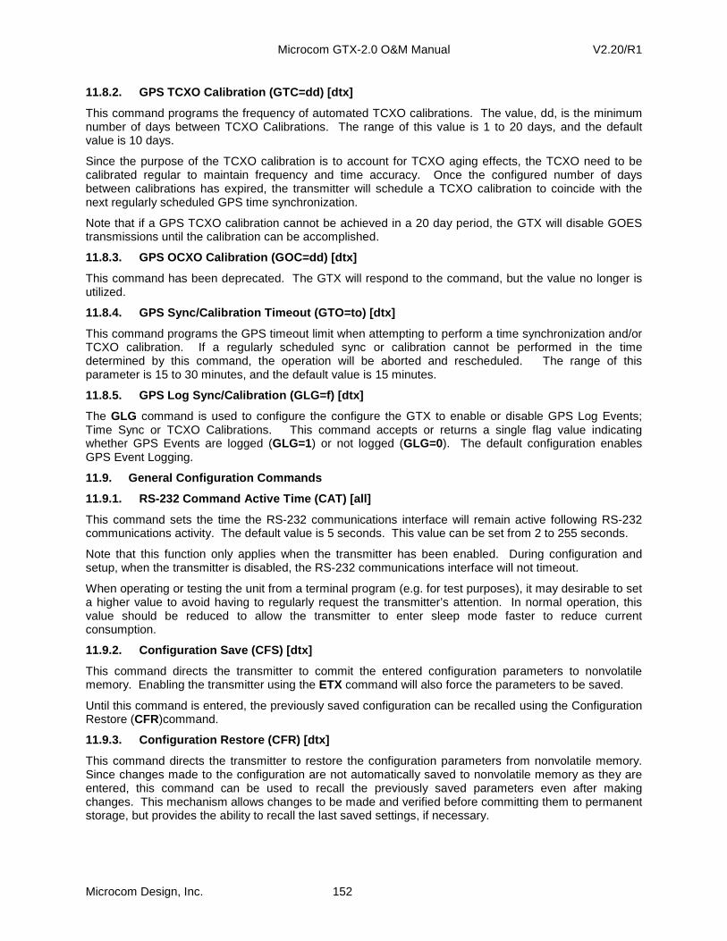
Microcom GTX-2.0 O&M Manual V2.20/R1
Microcom Design, Inc. 152
11.8.2. GPS TCXO Calibration (GTC=dd) [dtx]
This command programs the frequency of automated TCXO calibrations. The value, dd, is the minimum number of days between TCXO Calibrations. The range of this value is 1 to 20 days, and the default value is 10 days.
Since the purpose of the TCXO calibration is to account for TCXO aging effects, the TCXO need to be calibrated regular to maintain frequency and time accuracy. Once the configured number of days between calibrations has expired, the transmitter will schedule a TCXO calibration to coincide with the next regularly scheduled GPS time synchronization.
Note that if a GPS TCXO calibration cannot be achieved in a 20 day period, the GTX will disable GOES transmissions until the calibration can be accomplished.
11.8.3. GPS OCXO Calibration (GOC=dd) [dtx]
This command has been deprecated. The GTX will respond to the command, but the value no longer is utilized.
11.8.4. GPS Sync/Calibration Timeout (GTO=to) [dtx]
This command programs the GPS timeout limit when attempting to perform a time synchronization and/or TCXO calibration. If a regularly scheduled sync or calibration cannot be performed in the time determined by this command, the operation will be aborted and rescheduled. The range of this parameter is 15 to 30 minutes, and the default value is 15 minutes.
11.8.5. GPS Log Sync/Calibration (GLG=f) [dtx]
The GLG command is used to configure the configure the GTX to enable or disable GPS Log Events; Time Sync or TCXO Calibrations. This command accepts or returns a single flag value indicating whether GPS Events are logged (GLG=1) or not logged (GLG=0). The default configuration enables GPS Event Logging.
11.9. General Configuration Commands
11.9.1. RS-232 Command Active Time (CAT) [all]
This command sets the time the RS-232 communications interface will remain active following RS-232 communications activity. The default value is 5 seconds. This value can be set from 2 to 255 seconds.
Note that this function only applies when the transmitter has been enabled. During configuration and setup, when the transmitter is disabled, the RS-232 communications interface will not timeout.
When operating or testing the unit from a terminal program (e.g. for test purposes), it may desirable to set a higher value to avoid having to regularly request the transmitter’s attention. In normal operation, this value should be reduced to allow the transmitter to enter sleep mode faster to reduce current consumption.
11.9.2. Configuration Save (CFS) [dtx]
This command directs the transmitter to commit the entered configuration parameters to nonvolatile memory. Enabling the transmitter using the ETX command will also force the parameters to be saved.
Until this command is entered, the previously saved configuration can be recalled using the Configuration Restore (CFR)command.
11.9.3. Configuration Restore (CFR) [dtx]
This command directs the transmitter to restore the configuration parameters from nonvolatile memory. Since changes made to the configuration are not automatically saved to nonvolatile memory as they are entered, this command can be used to recall the previously saved parameters even after making changes. This mechanism allows changes to be made and verified before committing them to permanent storage, but provides the ability to recall the last saved settings, if necessary.
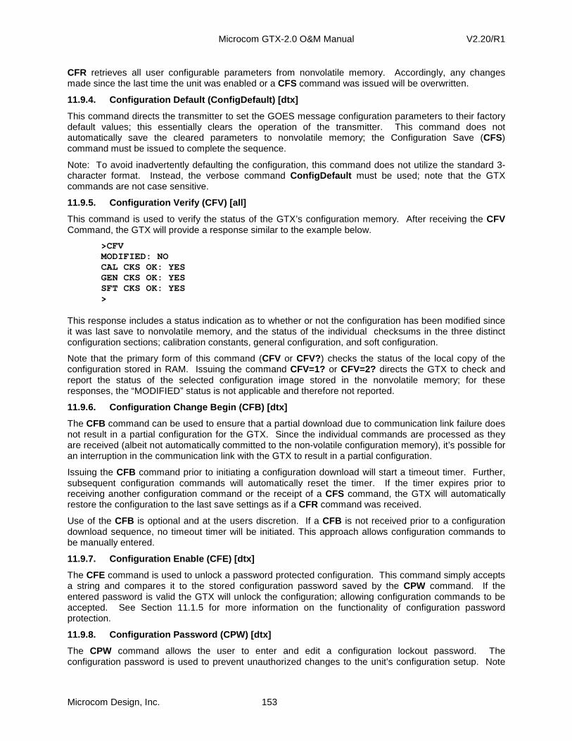
Microcom GTX-2.0 O&M Manual V2.20/R1
Microcom Design, Inc. 153
CFR retrieves all user configurable parameters from nonvolatile memory. Accordingly, any changes made since the last time the unit was enabled or a CFS command was issued will be overwritten.
11.9.4. Configuration Default (ConfigDefault) [dtx]
This command directs the transmitter to set the GOES message configuration parameters to their factory default values; this essentially clears the operation of the transmitter. This command does not automatically save the cleared parameters to nonvolatile memory; the Configuration Save (CFS) command must be issued to complete the sequence.
Note: To avoid inadvertently defaulting the configuration, this command does not utilize the standard 3-character format. Instead, the verbose command ConfigDefault must be used; note that the GTX commands are not case sensitive.
11.9.5. Configuration Verify (CFV) [all]
This command is used to verify the status of the GTX’s configuration memory. After receiving the CFV Command, the GTX will provide a response similar to the example below.
>CFV MODIFIED: NO CAL CKS OK: YES GEN CKS OK: YES SFT CKS OK: YES >
This response includes a status indication as to whether or not the configuration has been modified since it was last save to nonvolatile memory, and the status of the individual checksums in the three distinct configuration sections; calibration constants, general configuration, and soft configuration.
Note that the primary form of this command (CFV or CFV?) checks the status of the local copy of the configuration stored in RAM. Issuing the command CFV=1? or CFV=2? directs the GTX to check and report the status of the selected configuration image stored in the nonvolatile memory; for these responses, the “MODIFIED” status is not applicable and therefore not reported.
11.9.6. Configuration Change Begin (CFB) [dtx]
The CFB command can be used to ensure that a partial download due to communication link failure does not result in a partial configuration for the GTX. Since the individual commands are processed as they are received (albeit not automatically committed to the non-volatile configuration memory), it’s possible for an interruption in the communication link with the GTX to result in a partial configuration.
Issuing the CFB command prior to initiating a configuration download will start a timeout timer. Further, subsequent configuration commands will automatically reset the timer. If the timer expires prior to receiving another configuration command or the receipt of a CFS command, the GTX will automatically restore the configuration to the last save settings as if a CFR command was received.
Use of the CFB is optional and at the users discretion. If a CFB is not received prior to a configuration download sequence, no timeout timer will be initiated. This approach allows configuration commands to be manually entered.
11.9.7. Configuration Enable (CFE) [dtx]
The CFE command is used to unlock a password protected configuration. This command simply accepts a string and compares it to the stored configuration password saved by the CPW command. If the entered password is valid the GTX will unlock the configuration; allowing configuration commands to be accepted. See Section 11.1.5 for more information on the functionality of configuration password protection.
11.9.8. Configuration Password (CPW) [dtx]
The CPW command allows the user to enter and edit a configuration lockout password. The configuration password is used to prevent unauthorized changes to the unit’s configuration setup. Note
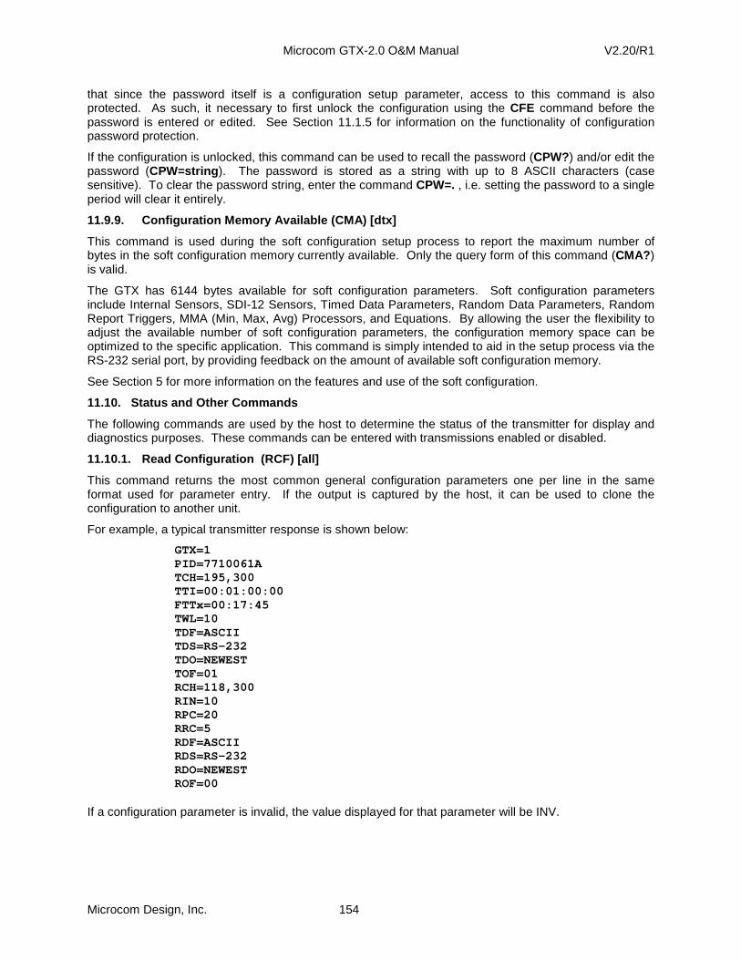
Microcom GTX-2.0 O&M Manual V2.20/R1
Microcom Design, Inc. 154
that since the password itself is a configuration setup parameter, access to this command is also protected. As such, it necessary to first unlock the configuration using the CFE command before the password is entered or edited. See Section 11.1.5 for information on the functionality of configuration password protection.
If the configuration is unlocked, this command can be used to recall the password (CPW?) and/or edit the password (CPW=string ). The password is stored as a string with up to 8 ASCII characters (case sensitive). To clear the password string, enter the command CPW=. , i.e. setting the password to a single period will clear it entirely.
11.9.9. Configuration Memory Available (CMA) [dtx]
This command is used during the soft configuration setup process to report the maximum number of bytes in the soft configuration memory currently available. Only the query form of this command (CMA? ) is valid.
The GTX has 6144 bytes available for soft configuration parameters. Soft configuration parameters include Internal Sensors, SDI-12 Sensors, Timed Data Parameters, Random Data Parameters, Random Report Triggers, MMA (Min, Max, Avg) Processors, and Equations. By allowing the user the flexibility to adjust the available number of soft configuration parameters, the configuration memory space can be optimized to the specific application. This command is simply intended to aid in the setup process via the RS-232 serial port, by providing feedback on the amount of available soft configuration memory.
See Section 5 for more information on the features and use of the soft configuration.
11.10. Status and Other Commands
The following commands are used by the host to determine the status of the transmitter for display and diagnostics purposes. These commands can be entered with transmissions enabled or disabled.
11.10.1. Read Configuration (RCF) [all]
This command returns the most common general configuration parameters one per line in the same format used for parameter entry. If the output is captured by the host, it can be used to clone the configuration to another unit.
For example, a typical transmitter response is shown below:
GTX=1 PID=7710061A TCH=195,300 TTI=00:01:00:00 FTTx=00:17:45 TWL=10 TDF=ASCII TDS=RS-232 TDO=NEWEST TOF=01 RCH=118,300 RIN=10 RPC=20 RRC=5 RDF=ASCII RDS=RS-232 RDO=NEWEST ROF=00
If a configuration parameter is invalid, the value displayed for that parameter will be INV.
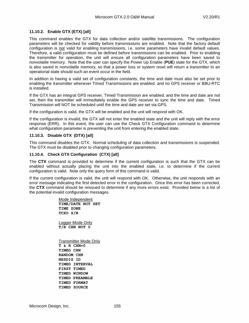
Microcom GTX-2.0 O&M Manual V2.20/R1
Microcom Design, Inc. 155
11.10.2. Enable GTX (ETX) [all]
This command enables the GTX for data collection and/or satellite transmissions. The configuration parameters will be checked for validity before transmissions are enabled. Note that the factory default configuration is not valid for enabling transmissions, i.e. some parameters have invalid default values. Therefore, a valid configuration must be defined before transmissions can be enabled. Prior to enabling the transmitter for operation, the unit will ensure all configuration parameters have been saved to nonvolatile memory. Note that the user can specify the Power Up Enable (PUE) state for the GTX, which is also saved in nonvolatile memory, so that a power loss or system reset will return a transmitter to an operational state should such an event occur in the field.
In addition to having a valid set of configuration constants, the time and date must also be set prior to enabling the transmitter whenever Timed Transmissions are enabled, and no GPS receiver or BBU-RTC is installed.
If the GTX has an integral GPS receiver, Timed Transmission are enabled, and the time and date are not set, then the transmitter will immediately enable the GPS receiver to sync the time and date. Timed Transmission will NOT be scheduled until the time and date are set via GPS.
If the configuration is valid, the GTX will be enabled and the unit will respond with OK.
If the configuration is invalid, the GTX will not enter the enabled state and the unit will reply with the error response (ERR). In this event, the user can use the Check GTX Configuration command to determine what configuration parameter is preventing the unit from entering the enabled state.
11.10.3. Disable GTX (DTX) [all]
This command disables the GTX. Normal scheduling of data collection and transmissions is suspended. The GTX must be disabled prior to changing configuration parameters.
11.10.4. Check GTX Configuration (CTX) [all]
The CTX command is provided to determine if the current configuration is such that the GTX can be enabled without actually placing the unit into the enabled state, i.e. to determine if the current configuration is valid. Note only the query form of this command is valid.
If the current configuration is valid, the unit will respond with OK. Otherwise, the unit responds with an error message indicating the first detected error in the configuration. Once this error has been corrected, the CTX command should be reissued to determine if any more errors exist. Provided below is a list of the potential invalid configuration messages.
Mode Independent TIME/DATE NOT SET TIME ZONE TCXO S/N Logger Mode Only T/R CHN NOT 0 Transmitter Mode Only T & R CHN=0 TIMED CHN RANDOM CHN NESDIS ID TIMED INTERVAL FIRST TIMED TIMED WINDOW TIMED PREAMBLE TIMED FORMAT TIMED SOURCE

Microcom GTX-2.0 O&M Manual V2.20/R1
Microcom Design, Inc. 156
TIMED ORDER TIME/DATE NOT SET TIMED BUFFER RANDOM PREAMBLE RANDOM FORMAT RANDOM SOURCE RANDOM ORDER RANDOM INTERVAL RANDOM PERCENT RANDOM REPEAT RANDOM BUFFER RANDOM BUFFER SIZE
If the CTX command is issued with the transmitter enabled, the unit will respond with CTX=GTX Enabled .
If the response is either the “TIMED BUFFER” or the “RANDOM BUFFER” error message, then there is an error in one or more data parameter definitions for the corresponding transmit buffer. In this event, the user can use the TDP or RDP command (with a question mark) to determine which parameter(s) are in error.
11.10.5. Read Status (RST) [all]
This command returns the firmware version # (M designates the Main Microcontroller firmware revision, while T designates the TKM firmware revision), serial number, transmitter state, GPS state, time to next transmission, number of bytes in timed transmit buffer, number of bytes in random transmit buffer, number of random transmission still pending, and the failsafe status.
The transmitter responds with:
FirmwareVersions: Mm.mm,Tt.t SerialNumber: nnnn TransmitterState: Enabled/Disabled GPSState: <status> TimeToNextTx: dd:hh:mm:ss TimedBufferSize: nnnn NextTimedTx: N/A or mm/dd/yyyy hh:mm:ss RandomBufferSize: nnnn RandomBufferTxs: nnn NextRandomTx: N/A or mm/dd/yyyy hh:mm:ss FailSafe: OK/Tripped
An additional feature of this comand is the auto status dump. Issuing the GTX the command RST=AUTO will direct the GTX to continuously dump the status report every few seconds (i.e. without being requested). Once this mode is enabled, the user must an an ESC to terminate the mode and allow new commands to be entered.
11.10.6. Last Transmission Status (LTS) [all]
This command returns the status of the last transmission. The last transmission could have been a regularly scheduled timed transmission, a random transmission, or a test transmission triggered by the FTX command.
If a transmission has occurred since the unit was last powered up, the transmitter responds to the command with:
TxType: Timed/Random/Test TxStatus: OK/FAIL TxTime: hh:mm:ss TxDate: mm/dd/yyyy FwdPwr: xx.x dBW RevPwr: xx.x dBW

Microcom GTX-2.0 O&M Manual V2.20/R1
Microcom Design, Inc. 157
TxVSWR: xx.xx:1 TxVolts: vv.v V >
Note: If the VSWR measures above 10:1, then the TxVSWR reading will indicate this condition with the string ” > 10:1 ”.
If no transmission has occurred, the response is just:
TxType: None In place of the generic failure response (“FAIL”), the transmitter may respond with one of the four specific failure indications:
TxStatus: FAILSAFE ⇒⇒⇒⇒ failsafe tripped TxStatus: FAIL POWER ⇒⇒⇒⇒ battery volts outside limits TxStatus: FAIL SYNTHESIZER ⇒⇒⇒⇒ frequency synthesizer unable to lock TxStatus: FAIL TEMPERATURE ⇒⇒⇒⇒ temperature outside transmit limits
Setting the Status Dump bit in either the TimedOpFlags (see Section 11.2.7) or the RandomOpFlags (see Section 11.2.19) will direct the transmitter to dump this information following a self-timed or random satellite transmission, respectively. Either of these flags being set will initiate the status report following a test transmission.
11.10.7. Transmission Summary Counts (TXC) [all]
The TXC command is used to clear or recall the GTX’s Good and Bad Transmission counts. The GTX keeps two sets of good/bad counts; one for Self-Timed transmission and another for Random transmissions. After each transmission, the GTX will increment the appropriate count based on the type of transmission and whether or not the transmission completed successfully.
The TXC or TXC? commands return the four count values separated by commas as shown in the example below. The first two values are the number of Good and Bad Self-Timed Transmissions (e.g. 147 Good and 2 Bad), while the second two values are the counts for Random Transmissions (e.g. 26 Good and no Bad).
>TXC? TXC=147,2,26,0 >
Issuing TXC=CLEAR (keyword CLEAR must be uppercase) will reset all four counts to zero. Note the Tx Good and Bad counts are also automatically cleared on power up; however, the values are not cleared when the GTX is enabled or disabled.
11.10.8. GPS Module On/Off (GPO) [dtx]
The GPO command allows the user to manually energize the GPS receiver for test and troubleshooting purposes when the GTX is disabled.
Issuing GPO=1 will turn on the GPS receiver and issuing GPO=0 will turn off the GPS receiver.
Using the query form of the command (GPO?) will return the current on/off state of the GPS receiver (1/0, respectively).
11.10.9. GPS State (GPS) [all]
This command returns a string indicating the current GPS state. This is the same information as provided in the “GPSState” field in response to the RST command. The string returned is one of the following.
Not Installed Off On-Initializing

Microcom GTX-2.0 O&M Manual V2.20/R1
Microcom Design, Inc. 158
On-No Usable Sats On-Need GPS Time On-1 Sat On-2 Sats On-3 Sats On-Waiting Solution On-Pos Fixes, Need UTC Corr On-Pos Fixes On-Unknown State
11.10.10. GPS Extended Status (GPX) [all]
The GPX command is an extended version of the GPS status request. This command returns additional information on the health and operation mode of the GPS module.
If the GPS receiver is off, then this command will simply return the string below.
GPX=Off
If the GPS receiver is on, then this command will return four lines similar to the example shown below.
GPS: On-Pos Fixes Fix: 3D Sat: 5 Ant: OK
The “GPS” field is the current GPS state string, which will be one of those shown in Section 11.10.9.
The “Fix” mode will be either 2D or 3D when the GPS receiver is performing position fixes and will be “?D” otherwise.
The “Sat” is the total number of GPS satellites currently being tracked.
The “Ant” field reports the health of the GPS Antenna. If a fault is detected in the GPS antenna, the “Ant” status line will report either “Open” (no antenna connected) or “Short” (the anntena and/or cable appears as an electrical short); otherwise, the “Ant” field will report as “OK”.
11.10.11. GPS Version (GPV) [all]
This command can be used to query the GPS receiver for its current firmware version. In order to retrieve this information, the GPS module MUST be on. Provided below is an example response.
GPV=C1.30 11.10.12. GPS Satellite Status (GSS) [all]
The GSS command allows the user to query the current GPS Satellite Status information. Specifically, this command provides a list of the GPS satellites currently being tracked and their respective ID number, azimuth, elevation, received signal quality, and a flag that indicates whether or not this satellite is currently being used in the position solution. The GPS receiver can track up to 12 satellites at any given instant, and the response to this command is a single line for each of the possible twelve satellites that can be tracked.
Each line is annotated with a satellite label after which is provided the data for the satellite. The first filed is the GPS Satellite ID (or PRN) number in the GPS constellation. Next is the Azimuth (0-90º) and Elevation (0-359º) of the satellite in degrees. The fourth field is the received Signal-to-Noise Ratio (SNR, aka C/N0); SNR is reported in decibels (dB). The final filed is a ‘1’ or ‘0’ indicating whether this satellite “is” or “is not” being used in the position solution, respectively. If a field value is unknown, it is reported with hyphens.
Provided below is an example of a typical response to the GSS command. In this example, of the twelve possible satellites, only eleven are currently being reported as being tracked or expected to be in view. As such, SAT12 is not reporting any numerical values in the first four fields, instead hyphens are reported

Microcom GTX-2.0 O&M Manual V2.20/R1
Microcom Design, Inc. 159
in these fields. Further, ten of the eleven satellites are currently being tracked; specifically, SAT01 thru SAT06 and SAT08 thru SAT11. Of these ten satellites all but SAT11 is being used in the solution. The SNRs for the acquired satellites range from 33 dB (SAT10) to 51 (SAT05).
>GSS SAT01: 21,61,207,49,1 SAT02: 24,58,105,49,1 SAT03: 15,38,054,47,1 SAT04: 22,37,302,47,1 SAT05: 14,25,245,51,1 SAT06: 09,13,038,49,1 SAT07: 33,13,109,--,0 SAT08: 06,10,279,44,1 SAT09: 19,07,317,45,1 SAT10: 03,05,294,33,1 SAT11: 18,--,---,50,0 SAT12: --,--,---,--,0
While SAT07’s Azimuth and Elevation are known from the almanac data provide by the GPS constellation, it is currently not being tracked as indicated by the absent SNR field. Conversely, SAT11 is currently being tracked, but the GPS module doesn’t have sufficient information to determine its Azimuth and Elevation.
Naturally, the satellite status only available when the GPS receiver is on. When the GPS receiver is off (GPO=0), the response to the command will be in the same format as shown above, but all twelve satellites will report null data similar to the way SAT12 is being reported in the example above.
The satellite signal strength information is automatically updated every second.
11.10.13. GPS Clock Check (GCC) [all]
The GCC command provides the ability to determine how far off the GTX’s internal clock from UTC. The query form of the command (GCC?) simply returns the date and time the last check was made and the clock error in seconds. The clock check information is captured whenever an automatic time sync is made or can be manually captured using the execute form of the command (GCC).
To manually capture the clock error, the GTX must be disabled (so as to not interfere with automatic updates), and the GPS receiver must be powered up and doing position fixes. Below is an example of how to use the GCC command. In this example, the GTX’s clock is currently 7 milliseconds ahead of UTC.
>GPO=1 OK >GPS? GPS=On-Pos Fixes >GCC GCC=09/15/2010 16:55:56,+0.007 >
11.10.14. Read GPS Position (RGP) [all]
This command returns the status of the last GPS fix whether it was a regularly scheduled fix or triggered by a Force GPS Fix command. The status parameters returned include: the time and date of the fix, latitude, longitude, and altitude. For this command the latitude and longitude are reported in degrees (with a leading sign character, ‘s’), minutes, and seconds. For the latitude, ‘+’ indicates North and ‘–‘ indicates South; while for longitude, ‘+’ indicates East and ‘–‘ indicates West. Altitude is reported in meters.
If a GPS fix has not yet occurred the transmitter will respond with: TOF: No Fix
Otherwise, it will respond with:
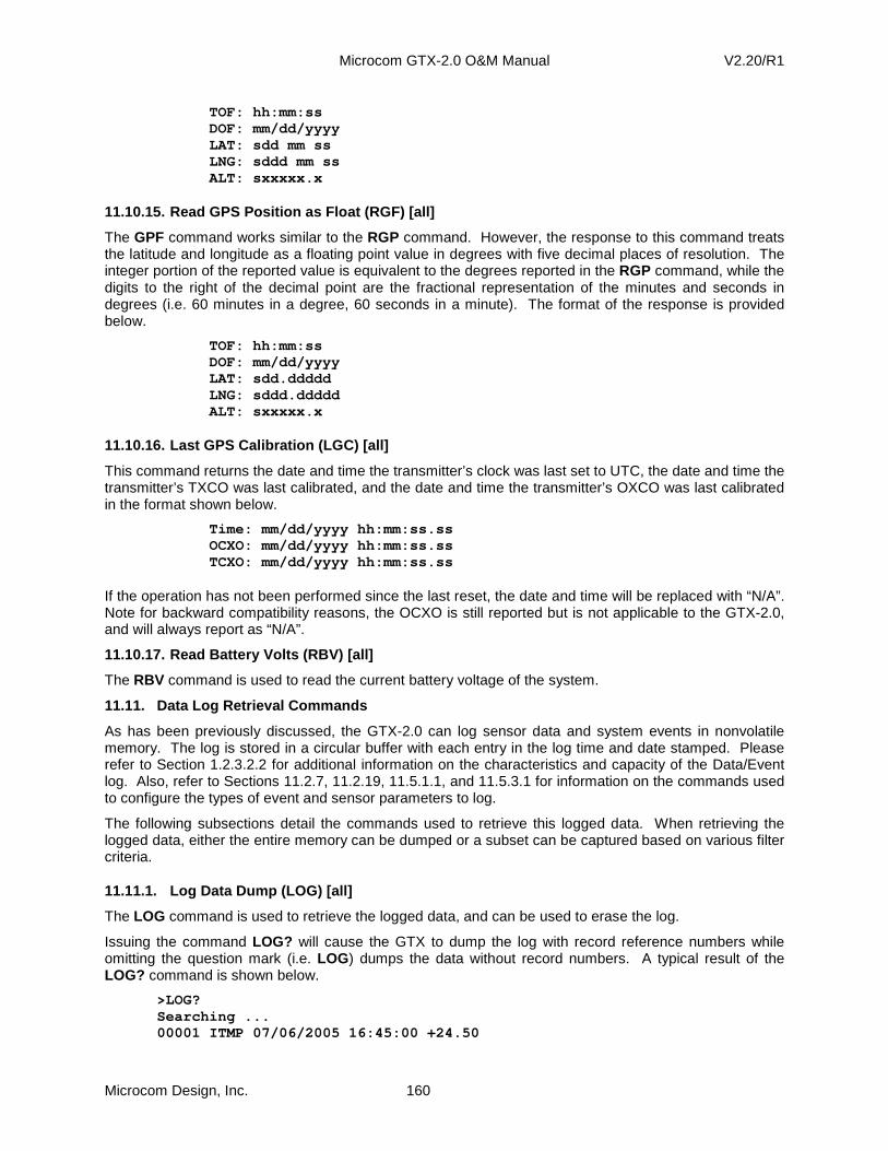
Microcom GTX-2.0 O&M Manual V2.20/R1
Microcom Design, Inc. 160
TOF: hh:mm:ss DOF: mm/dd/yyyy LAT: sdd mm ss LNG: sddd mm ss ALT: sxxxxx.x
11.10.15. Read GPS Position as Float (RGF) [all]
The GPF command works similar to the RGP command. However, the response to this command treats the latitude and longitude as a floating point value in degrees with five decimal places of resolution. The integer portion of the reported value is equivalent to the degrees reported in the RGP command, while the digits to the right of the decimal point are the fractional representation of the minutes and seconds in degrees (i.e. 60 minutes in a degree, 60 seconds in a minute). The format of the response is provided below.
TOF: hh:mm:ss DOF: mm/dd/yyyy LAT: sdd.ddddd LNG: sddd.ddddd ALT: sxxxxx.x
11.10.16. Last GPS Calibration (LGC) [all]
This command returns the date and time the transmitter’s clock was last set to UTC, the date and time the transmitter’s TXCO was last calibrated, and the date and time the transmitter’s OXCO was last calibrated in the format shown below.
Time: mm/dd/yyyy hh:mm:ss.ss OCXO: mm/dd/yyyy hh:mm:ss.ss TCXO: mm/dd/yyyy hh:mm:ss.ss
If the operation has not been performed since the last reset, the date and time will be replaced with “N/A”. Note for backward compatibility reasons, the OCXO is still reported but is not applicable to the GTX-2.0, and will always report as “N/A”.
11.10.17. Read Battery Volts (RBV) [all]
The RBV command is used to read the current battery voltage of the system.
11.11. Data Log Retrieval Commands
As has been previously discussed, the GTX-2.0 can log sensor data and system events in nonvolatile memory. The log is stored in a circular buffer with each entry in the log time and date stamped. Please refer to Section 1.2.3.2.2 for additional information on the characteristics and capacity of the Data/Event log. Also, refer to Sections 11.2.7, 11.2.19, 11.5.1.1, and 11.5.3.1 for information on the commands used to configure the types of event and sensor parameters to log.
The following subsections detail the commands used to retrieve this logged data. When retrieving the logged data, either the entire memory can be dumped or a subset can be captured based on various filter criteria.
11.11.1. Log Data Dump (LOG) [all]
The LOG command is used to retrieve the logged data, and can be used to erase the log.
Issuing the command LOG? will cause the GTX to dump the log with record reference numbers while omitting the question mark (i.e. LOG) dumps the data without record numbers. A typical result of the LOG? command is shown below.
>LOG? Searching ... 00001 ITMP 07/06/2005 16:45:00 +24.50

Microcom GTX-2.0 O&M Manual V2.20/R1
Microcom Design, Inc. 161
00002 TBCN 07/06/2005 16:45:02 00000 00003 WLVL 07/06/2005 16:45:09 +9.95 00004 ITMP 07/06/2005 17:00:00 +24.50 00005 WLVL 07/06/2005 17:00:09 +9.95 00006 STX 07/06/2005 17:02:30 TIMED 00007 ETX 07/06/2005 17:02:34 TIMED(b,f,r): 12.1,7 .7,-23.2 00008 ITMP 07/06/2005 17:15:00 +24.50 00009 WLVL 07/06/2005 17:15:09 +9.96 00010 ITMP 07/06/2005 17:30:00 +24.50 00011 WLVL 07/06/2005 17:30:09 +9.96 00012 TBCN 07/06/2005 17:32:02 00003 00013 TBCN 07/06/2005 17:44:02 00005 00014 ITMP 07/06/2005 17:45:00 +24.50 00015 WLVL 07/06/2005 17:45:09 +9.95 Total: 15 Dumped: 15 >
Each entry has 5-digit record number and a short string identifier. “STX” and ETX” identify the start and end of a transmission, respectively. The sensor labels defined by the SLX (Section 11.5.1.4) and ILX (Section 11.5.3.4) are used to identify the sensor readings. Following the identifier is the date and time the data was logged, and then the actual data is displayed.
For an “STX” entry, only the type of transmission (TEST, TIMED, or RANDOM) and the start time is logged. The “ETX” entry also includes the type of transmission, but additionally logs the transmission’s battery voltage (in VDC), and forward/reflected power readings (in dBW).
Two other types of events not shown in the list above can also be logged. These events (i.e. “SYNC” and “TCXO”) are related to GPS calibrations. The “SYNC” event identifies when the GTX’s internal clock was reset using the GPS and does not include any additional data. The “TCXO” event marks when the unit’s oscillator was re-calibrated using the GPS; this event also logs the absolute error from the expected nominal in parts per million (see Section 11.12.5 for additional information).
The only difference in the dump format for the LOG command is that no record numbers are provided. It should also be noted that with an expanded log memory (see Section 1.2.3.2.2) it is possible for the number of log entries to exceed 99,999, which means the record number could exceed five digits. For backward compatibility reason, the log dump preserved the 5-digit record number with leading zeroes. However, if the record number is 100,000 or higher then the record number will be reported with the appropriate number of digits.
The type of records dumped in response to LOG/LOG? commands can be controlled using the Log Filter command detailed in the next section.
Issuing LOG=CLEAR will direct the unit to completely erase the Data/Event log.
11.11.2. Log Filter Control (LFX) [all]
The LFX (X=A, B, T, S, I, D, or *) command can be used to define filter criteria for log dumps. Data can be filtered on date/time, type, and/or by a particular set of sensors.
LFA=date[,time] and LFB=date[,time] are used to define an after and/or before date/time filter. The time is optional; if omitted, the time will default to midnight (i.e. 00:00:00). Setting only LFA, dumps all records after the specified date/time; setting only LFB, dumps all records before the specified date/time. Setting both defines a date/time range.
LFT is used to limit the dump to one of the two main entry types. LFT=D selects only sensor data entries, LFT=E selects only event entries.
LFS=<subset> and LFI=<subset> , are used to select a subset of SDI-12 Sensors and/or a subset of Internal Sensors. The <subset> list can specify a single sensor, a range of sensors, or a list of sensors. For this command, sensors are always specified by their sensor number (0-63 for SDI-12 and 0-63 for Internal). To specify a range, a start and end sensor number separated by a dash is provided (e.g. 2-4).
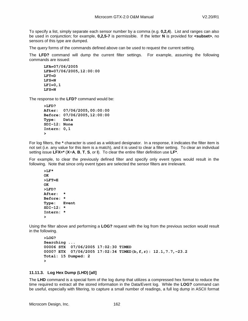
Microcom GTX-2.0 O&M Manual V2.20/R1
Microcom Design, Inc. 162
To specify a list, simply separate each sensor number by a comma (e.g. 0,2,4). List and ranges can also be used in conjunction; for example, 0,2,5-7 is permissible. If the letter N is provided for <subset> , no sensors of this type are dumped.
The query forms of the commands defined above can be used to request the current setting.
The LFD? command will dump the current filter settings. For example, assuming the following commands are issued:
LFA=07/06/2005 LFB=07/06/2005,12:00:00 LFT=D LFS=N LFI=0,1 LFS=N
The response to the LFD? command would be:
>LFD? After: 07/06/2005,00:00:00 Before: 07/06/2005,12:00:00 Type: Data SDI-12: None Intern: 0,1 >
For log filters, the * character is used as a wildcard designator. In a response, it indicates the filter item is not set (i.e. any value for this item is a match), and it is used to clear a filter setting. To clear an individual setting issue LFX=* (X=A, B, T, S, or I). To clear the entire filter definition use LF*.
For example, to clear the previously defined filter and specify only event types would result in the following. Note that since only event types are selected the sensor filters are irrelevant.
>LF* OK >LFT=E OK >LFD? After: * Before: * Type: Event SDI-12: * Intern: * >
Using the filter above and performing a LOG? request with the log from the previous section would result in the following.
>LOG? Searching ... 00006 STX 07/06/2005 17:02:30 TIMED 00007 ETX 07/06/2005 17:02:34 TIMED(b,f,r): 12.1,7 .7,-23.2 Total: 15 Dumped: 2 >
11.11.3. Log Hex Dump (LHD) [all]
The LHD command is a special form of the log dump that utilizes a compressed hex format to reduce the time required to extract all the stored information in the Data/Event log. While the LOG? command can be useful, especially with filtering, to capture a small number of readings, a full log dump in ASCII format

Microcom GTX-2.0 O&M Manual V2.20/R1
Microcom Design, Inc. 163
can take a substantial amount time to complete due to the verboseness of each line. The compressed data dump from this command will typically require only 1/5 the total time as an ASCII dump of the log. This command does not filter the data, all data entries are included regardless of the filtering option specified.
While the specifics required to parse out this data is proprietary and not documented in this manual, this command can still be useful as Microcom provides at no charge a separate utility to parse out the data from a captured text file. In other words, this command can be used to get a quick dump of the entire log and capture the data to a text file, which can then be input to the parsing utility for decompression. Note that the Configuration Utility actually utilizes this command when no filtering is active.
Below is an example of a short hex dump.
>LHD? 000049 300A5EC70C060062B28207000090870A 03E3F0037B0062D08903E381008D0482 84047904DF18F002EA0062D08903E4F0 037B0062D08903E4F2F10003F202D000 05F0BA0062D08903E3FFFFFFFFFFFFFF >
Please contact Microcom Design to obtain the parsing utility and to get additional information on its use.
11.11.4. Log Hex Filter Dump (LHF) [all]
The LHF command is a special form of the log dump that utilizes a compressed hex format to reduce the time required to dump specific records from the Data/Event log. The LHF command is similar to the LHD command described in the previous section, except that the currently defined filtering is applied (see Section 11.11.2). While the LOG? command can be useful, especially with filtering, to capture a small number of readings, even a large filtered dump can take time. The compressed data dump from this command can significantly reduce this time by allowing only specific records to be dumped.
While the specifics required to parse out this data is proprietary and not documented in this manual, this command can still be useful as Microcom provides at no charge a separate utility to parse out the data from a captured text file. In other words, this command can be used to get a quick filtered dump from the log, and the data captured to a text file, which can then be input to the parsing utility for decompression. Note that Configuration Utility actually utilizes this command when filtering is active.
Below is an example of a short, filtered hex dump.
>LHF? 300A5EC70C060062 320A5EC70E070000 100A5EC7150A03E3 300A5ECA90060062 100A5ECA990A03E3 300A5ECE14060062 100A5ECE1D0A03E4 300A5ED198060062 100A5ED1A10A03E4 320A5ED212070003 320A5ED4E2070005 300A5ED51C060062 100A5ED5250A03E3 >
Please contact Microcom Design to obtain the parsing utility and to get additional information on its use.

Microcom GTX-2.0 O&M Manual V2.20/R1
Microcom Design, Inc. 164
11.11.5. Auto Log Dump Monitor (LOG=AUTO) [all]
This special case of the LOG command allows the user to place the GTX in a special mode that dumps the Data/Event log entries to the serial port as they are stored in the buffer. In other words, this mode allows active and automatic monitoring of the logging process. To enable this mode, the LOG command must be entered with the special keyword AUTO (uppercase only) as its only parameter (i.e. LOG=AUTO ).
While the GTX provides other test mechanisms to monitor sensor sampling (see Section 11.5.1.6 and 11.5.3.6), the sensor sampling functions are not selectable to an individual sensor, i.e. only all Internal Sensors and/or all SDI-12 sensors can be monitored with these commands. The LOG=AUTO function on the other hand is subject to the Log Filtering functions described in Section 11.11.2. While all data is still logged, only the parameters that meet the filter criteria will be echoed to the serial port. As such, the user can use this feature to monitor a specific set of sensors. Once this mode is enabled, the user must issue an ESC to terminate the mode and allow new commands to be entered.
11.11.6. Log Memory Size (LGS) [all]
The logging memory of the GTX-2.0 can be expanded from the standard 128 kilobytes to as much as 1 megabyte (in 128 kB steps). After power up, the GTX automatically determines the total logging memory available. This query form of this command returns the total size in bytes, number of bytes currently in use, and the number of bytes available. Format of the response is provided below:
>LGS? LGS=<total>,<used>,<free>
NOTE: Since the Data/Event log uses a circular storage approach, the free amount does NOT have any
bearing on the number of future entries that can be saved; instead it simply provides the amount of currently unused memory.
11.12. Transmitter Test Commands
The following commands are used for testing the transmitter during troubleshooting. These commands can only be entered when normal transmissions are disabled. The test results are returned using the status commands listed in the previous sections.
11.12.1. Force Test Transmission (FTX=type,channel, bitrate) [dtx]
Force the immediate transmission of a test message.
Parameters:
type: 1 or C for carrier only 2 or K for alternating 010101 modulation (a.k.a. clock) 3 or R for random modulation 4 or M for fixed message with contents “FIELD INITIATED TEST TRANSMISSION”. 5 or I for identification message.
channel: 1 – 266 for bit rates of 100 and 300 1 – 133 for a bit rate of 1200 bitrate: 100, 300 or 1200 bps
Normal transmissions must be disabled using the DisableTx command for this command to work. Test transmission types 1 (C), 2 (K) and 3 (R) will continue until the StopTx command is received. Test transmission types 4 (M) and 5 (I) will stop as soon as the message transmission is completed.
The identification message (5 or I) includes the Platform ID string (PIS, 11.7.3.1.1); the fixed message string as in type 4 or M; and the GPS position information (latitude and longitude), if available.
It should also be noted that tripping the failsafe does not automatically terminate a continuous RF mode, an STX command must still be issued to disable the modulator. In other words, since only the final RF output stage is disabled via the independent failsafe mechanism, the transmitter internally continues to generate the requested modulation. Accordingly, resetting the failsafe without terminating a continuous
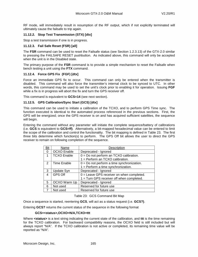
Microcom GTX-2.0 O&M Manual V2.20/R1
Microcom Design, Inc. 165
RF mode, will immediately result in resumption of the RF output, which if not explicitly terminated will ultimately cause the failsafe to trip again.
11.12.2. Stop Test Transmission (STX) [dtx]
Stop a test transmission if one is in progress.
11.12.3. Fail Safe Reset (FSR) [all]
The FSR command can be used to reset the Failsafe status (see Section 1.2.3.13) of the GTX-2.0 similar to pressing the FAILSAFE RESET pushbutton. As indicated above, this command will only be accepted when the unit is in the Disabled state.
The primary purpose of the FSR command is to provide a simple mechanism to reset the Failsafe when bench testing a unit using the FTX command.
11.12.4. Force GPS Fix (FGF) [dtx]
Force an immediate GPS fix to occur. This command can only be entered when the transmitter is disabled. This command will also force the transmitter’s internal clock to be synced to UTC. In other words, this command may be used to set the unit’s clock prior to enabling it for operation. Issuing FGF while a fix is in progress will abort the fix and turn the GPS receiver off.
This command is equivalent to GCS=14 (see next section).
11.12.5. GPS Calibration/Sync Start (GCS) [dtx]
This command can be used to initiate a calibration of the TCXO, and to perform GPS Time sync. The function executed is identical to the automated process referenced in the previous sections. First, the GPS will be energized; once the GPS receiver is on and has acquired sufficient satellites, the sequence will begin.
Entering the command without any parameter will initiate the complete sequence/battery of calibrations (i.e. GCS is equivalent to GCS=ff) . Alternatively, a bit-mapped hexadecimal value can be entered to limit the scope of the calibration and control the functionality. The bit mapping is defined in Table 23. The first three bits determine which function(s) to perform. The GPS Off bit allows the user to direct the GPS receiver to remain on following completion of the sequence.
Bit Name Description 0 OCXO Enable Deprecated - Ignored 1 TCXO Enable 0 = Do not perform an TCXO calibration.
1 = Perform an TCXO calibration. 2 Time Enable 0 = Do not perform a time synchronization.
1 = Perform a time synchronization. 3 Update Syn Deprecated - Ignored 4 GPS Off 0 = Leave GPS receiver on when completed.
1 = Turn GPS receiver off when completed. 5 OCXO Warm Up Deprecated - Ignored 6 Not used Reserved for future use 7 Not used Reserved for future use
Table 23: GCS Command Bit Map
Once a sequence is started, reentering GCS, will act as a status request (i.e. GCS?).
Entering GCS? returns the current status of the sequence in the following format
GCS=<status>,OCXO=N/A,TCXO=ttt
Where <status> is a text string indicating the current state of the calibration, and ttt is the time remaining for the TCXO calibration. For backward compatibility reasons, the OCXO field is still included but will always report “N/A”. If the TCXO calibration is not active or completed, its remaining time value will be reported as “N/A”.

Microcom GTX-2.0 O&M Manual V2.20/R1
Microcom Design, Inc. 166
To abort a calibration/time sync sequence, the command GCS=ABORT must be issued. The keyword ABORT must be in all caps.

Microcom GTX-2.0 O&M Manual V2.20/R1
Microcom Design, Inc. 167
12. Troubleshooting Hints
The GTX-2.0 and the Configuration Utility provides numerous troubleshooting tools to allow a user to diagnose problems. These tools not only provide diagnostic capabilities for the GTX itself, but also for devices connected to it (e.g. SDI-12 sensors).
While the GTX by itself provides significant self-diagnostic tools, users with numerous platforms (regardless of the manufacturer) may also benefit from the additional diagnostic capabilities provided by the Microcom GOES DCS Tx Test Set.
Section 12.1 provides information on using the basic tools provided by the GTX, while Section 12.2 provides an overview of the additional diagnostic capabilities inherent in the Microcom Test Set, especially those specifically intended for the GTX.
12.1. Using GTX and GTX Utility Tools
Included in the GTX’s command set are several commands specifically geared toward testing and troubleshooting a unit. Further, all of these diagnostic commands have been encapsulated in the Configuration Utility. Some of these features were discussed in previous sections. For example, Section 3.2.3 describes the Configuration Utility’s “Monitor/Inspect GTX” page, which provides a convenient mechanism to check status and diagnostic information for a myriad of GTX functions. Figure 17 in Section 3.3 shows how to use the Direct Control dialog in the Configuration Utility to gain low-level access to the GTX commands (i.e. provides an integrated terminal application). Simply retrieving the Data/Event log as discussed in Section 10 can be a useful diagnostic tool to identify intermittent problems and to verify a sensor is functioning properly.
This section will explain other useful diagnostic screens and expand on some of those already discussed.
12.1.1. Diagnostic Status Information
The GTX command set and Configuration Utility allow status information to be quickly gathered from a unit under test. For example, the LastTxStatus? command (see Section 11.10.6) provides useful information on the integrity of the transmit antenna connection as shown in Figure 80. This example also shows the GTX Direct Control dialog that allows GTX terminal commands to be issued.
Figure 80: Configuration Utility - Last Transmission Status Example
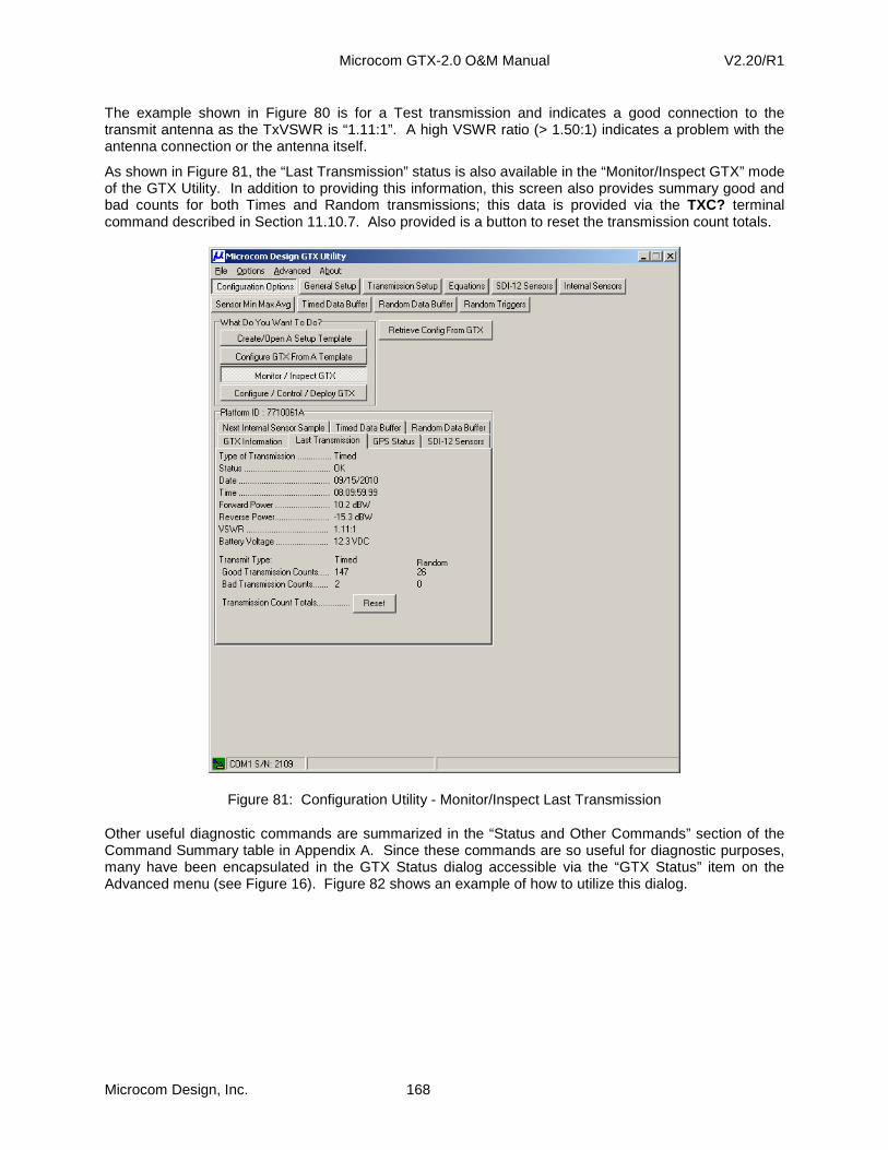
Microcom GTX-2.0 O&M Manual V2.20/R1
Microcom Design, Inc. 168
The example shown in Figure 80 is for a Test transmission and indicates a good connection to the transmit antenna as the TxVSWR is “1.11:1”. A high VSWR ratio (> 1.50:1) indicates a problem with the antenna connection or the antenna itself.
As shown in Figure 81, the “Last Transmission” status is also available in the “Monitor/Inspect GTX” mode of the GTX Utility. In addition to providing this information, this screen also provides summary good and bad counts for both Times and Random transmissions; this data is provided via the TXC? terminal command described in Section 11.10.7. Also provided is a button to reset the transmission count totals.
Figure 81: Configuration Utility - Monitor/Inspect Last Transmission
Other useful diagnostic commands are summarized in the “Status and Other Commands” section of the Command Summary table in Appendix A. Since these commands are so useful for diagnostic purposes, many have been encapsulated in the GTX Status dialog accessible via the “GTX Status” item on the Advanced menu (see Figure 16). Figure 82 shows an example of how to utilize this dialog.
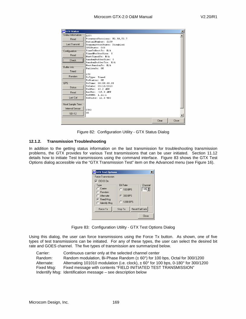
Microcom GTX-2.0 O&M Manual V2.20/R1
Microcom Design, Inc. 169
Figure 82: Configuration Utility - GTX Status Dialog
12.1.2. Transmission Troubleshooting
In addition to the getting status information on the last transmission for troubleshooting transmission problems, the GTX provides for various Test transmissions that can be user initiated. Section 11.12 details how to initiate Test transmissions using the command interface. Figure 83 shows the GTX Test Options dialog accessible via the “GTX Transmission Test” item on the Advanced menu (see Figure 16).
Figure 83: Configuration Utility - GTX Test Options Dialog
Using this dialog, the user can force transmissions using the Force Tx button. As shown, one of five types of test transmissions can be initiated. For any of these types, the user can select the desired bit rate and GOES channel. The five types of transmission are summarized below.
Carrier: Continuous carrier only at the selected channel center Random: Random modulation, Bi-Phase Random (± 60°) for 100 bps, Octal for 300/1200 Alternate: Alternating 101010 modulation (i.e. clock), ± 60° for 100 bps, 0-180° for 300/1200 Fixed Msg: Fixed message with contents “FIELD INITIATED TEST TRANSMISSION” Indentify Msg: Identification message – see description below

Microcom GTX-2.0 O&M Manual V2.20/R1
Microcom Design, Inc. 170
Note that normal transmissions must be disabled using the DisableTx command for this dialog to function. The first three Test transmission types will continue until the Stop Tx button is clicked, while the last two Test transmission types will stop as soon as the message transmission is completed.
The Identify Msg includes the Platform ID string (PIS, 11.7.3.1.1), the fixed message string as in the Fixed Msg type, and the GPS position information (latitude and longitude), if available.
Test transmissions are still subject to the GTX’s Failsafe Transmit Monitor. In other words, leaving continuous transmissions enabled for too long or sending transmissions too close together will trip the failsafe and disabling the RF output. For this reason, the Reset Fail-Safe button is provided. Note that this button will function only if the GTX has never been Enabled since the last time the power was recycled. Simply recycling the DC power will not necessarily allow the GTX to meet this requirement. The “Power Up Enabled” flag (see Section 3.4.2) must also be cleared so the GTX will not automatically enter the Enabled mode. The Reset Fail-Safe button can also be used in between transmission even if the Failsafe has not tripped to avoid tripping it on the next transmission.
It should also be noted that tripping the failsafe does not automatically terminate a continuous RF mode, the Stop Tx button must still be clicked. In other words, since only the final RF output stage is disabled via the independent failsafe mechanism, the transmitter internally continues to generate the requested modulation. Accordingly, resetting the failsafe without terminating a continuous RF mode, will immediately result in resumption of the RF output, which if not explicitly terminated will ultimately cause the failsafe to trip again.
NOTE: Forcing the GTX into a continuous Test mode f or an extended period of time can cause a significant temperature rise inside the unit, and c ould result in permanent damage. If it’s necessary, to enable the RF output for extended per iods of time (more than a minute), the units should be stood on its side and a fan provide d to force air circulation over the bottom of the case.

Microcom GTX-2.0 O&M Manual V2.20/R1
Microcom Design, Inc. 171
12.1.3. SDI-12 Troubleshooting
The GTX-2.0 provides several test modes to confirm proper operation of SDI-12 devices using the SDI12Test (SDI) command explained in Section 11.5.1.6.
To even further facilitate testing SDI-12 devices, the Configuration Utility provides the SDI-12 dialog shown in Figure 84. This dialog makes use of the SDI RS-232 command to send SDI-12 commands to devices connected to the bus. However, this command provides the added feature that it does not require the SDI-12 command to be preceded by “SDI=” as is required when using a Terminal interface or the GTX Direct Control dialog. When an SDI-12 command is entered in the top edit box (e.g. 0M), the Configuration Utility will insert the GTX command sequence and append the exclamation mark (e.g. SDI=0M!) before sending it to the GTX.
Figure 84: Configuration Utility - SDI-12 Dialog
If the Configuration Utility is placed in the Configure/Control/Deploy GTX mode (see Section 3.2.4), the SDI-12 Sensors page will look something like Figure 85. In this mode, the SDI-12 Sensor Query group is displayed. The Next Sample button can be used to query when the SDI-12 devices is next scheduled to be read.
Also, the Query Sensor button can be used to read the selected sensor. The selected sensor is indicated by the grid row that has a solid arrow in the left-most column. When the Query Sensor button is clicked, the Configuration Utility sends the appropriate {aMx} command, where a is Address and x is the Measurement specified in the grid. In other words, the sensor is queried exactly as it would be by the GTX when collecting data from this sensor.
Note that this function works even if the GTX is enabled for operation. However, if the SDI-12 bus is in use at the time the RS-232 command is received by the GTX, the sensor cannot be queried, as it would cause a bus collision. When this occurs, the GTX will respond with BUSY. Simply wait a moment and try again.

Microcom GTX-2.0 O&M Manual V2.20/R1
Microcom Design, Inc. 172
Figure 85: Configuration Utility - SDI-12 Sensors Page with Diagnostics
12.1.4. GPS Diagnostics
Numerous diagnostic, troubleshooting and calibration functions have been included in the GTX and the Utility. The following sections will detail these capabilities.
12.1.4.1. GPS Calibration
If an outside GPS antenna is available or a facility has an internal GPS repeater (GPS does not typically work indoors), then it’s possible to perform GPS diagnostics and calibrations on the bench. Since many facilities do not have this capability (i.e. access to a GPS antenna), the GTX Calibration menu option is disabled by default. To enable this option, go to the Calibration page of the Preferences dialog and check the “Show Calibration Menu” box. When enabled, the Advanced menu includes an additional option as shown in Figure 86.
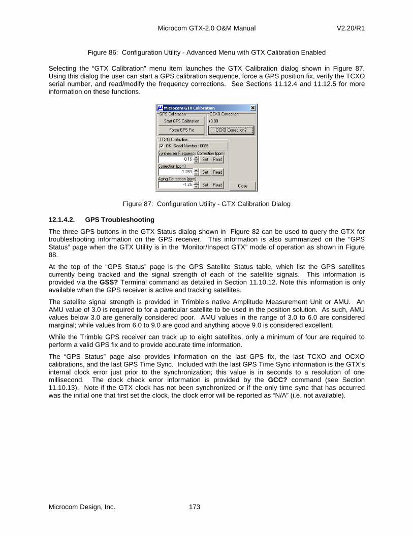
Microcom GTX-2.0 O&M Manual V2.20/R1
Microcom Design, Inc. 173
Figure 86: Configuration Utility - Advanced Menu with GTX Calibration Enabled
Selecting the “GTX Calibration” menu item launches the GTX Calibration dialog shown in Figure 87. Using this dialog the user can start a GPS calibration sequence, force a GPS position fix, verify the TCXO serial number, and read/modify the frequency corrections. See Sections 11.12.4 and 11.12.5 for more information on these functions.
Figure 87: Configuration Utility - GTX Calibration Dialog
12.1.4.2. GPS Troubleshooting
The three GPS buttons in the GTX Status dialog shown in Figure 82 can be used to query the GTX for troubleshooting information on the GPS receiver. This information is also summarized on the “GPS Status” page when the GTX Utility is in the “Monitor/Inspect GTX” mode of operation as shown in Figure 88.
At the top of the “GPS Status” page is the GPS Satellite Status table, which list the GPS satellites currently being tracked and the signal strength of each of the satellite signals. This information is provided via the GSS? Terminal command as detailed in Section 11.10.12. Note this information is only available when the GPS receiver is active and tracking satellites.
The satellite signal strength is provided in Trimble’s native Amplitude Measurement Unit or AMU. An AMU value of 3.0 is required to for a particular satellite to be used in the position solution. As such, AMU values below 3.0 are generally considered poor. AMU values in the range of 3.0 to 6.0 are considered marginal; while values from 6.0 to 9.0 are good and anything above 9.0 is considered excellent.
While the Trimble GPS receiver can track up to eight satellites, only a minimum of four are required to perform a valid GPS fix and to provide accurate time information.
The “GPS Status” page also provides information on the last GPS fix, the last TCXO and OCXO calibrations, and the last GPS Time Sync. Included with the last GPS Time Sync information is the GTX’s internal clock error just prior to the synchronization; this value is in seconds to a resolution of one millisecond. The clock check error information is provided by the GCC? command (see Section 11.10.13). Note if the GTX clock has not been synchronized or if the only time sync that has occurred was the initial one that first set the clock, the clock error will be reported as “N/A” (i.e. not available).
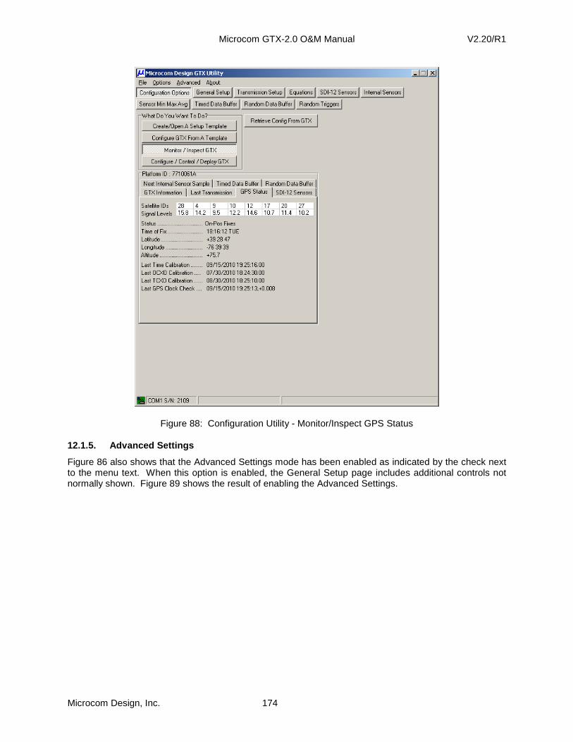
Microcom GTX-2.0 O&M Manual V2.20/R1
Microcom Design, Inc. 174
Figure 88: Configuration Utility - Monitor/Inspect GPS Status
12.1.5. Advanced Settings
Figure 86 also shows that the Advanced Settings mode has been enabled as indicated by the check next to the menu text. When this option is enabled, the General Setup page includes additional controls not normally shown. Figure 89 shows the result of enabling the Advanced Settings.

Microcom GTX-2.0 O&M Manual V2.20/R1
Microcom Design, Inc. 175
Figure 89: Configuration Utility - General Setup Page with Advanced Settings
In addition to the GPS Time Sync setting, the user can now adjust three additional parameters. These settings correspond to the GTC, GOC, and GTO commands. Information on the use and meaning of these configuration options can be found in Sections 11.8.2 through 11.8.4.
Also, as shown in Figure 89, the Advanced Settings group allows the user to modify the Invalid Character Replacement setting, which is equivalent to the IRC command (see Section 11.3.7). Further, this group box provides access to adjust the power settings in Watts for the transmitter for each of the three bps rates. The power settings can also be adjusted using the TXP command (see Section 11.3.1). Note that the maximum power setting is factory adjusted and limited based on the type of transmit antenna to be used based on NESDIS Certification requirements. Typically, the GTX is shipped with the desired output power equal to the maximum limit. Adjusting the power levels can be a useful diagnostic tool.
12.1.6. Antenna Pointing Aid
The GTX Utility has a built-in Antenna Pointing aid under the Advanced menu as shown in Figure 90. Selecting this menu option launches the GOES Antenna Pointing Utility dialog shown in Figure 91. This simple dialog makes it easy to get the correct Azimuth and Elevation angles for the transmit antenna based on a site’s latitude and longitude.
First the user needs to select the desired satellite; GOES East, GOES West, or a Custom satellite. Picking “GOES East” sets the “Target Satellite Longitude” to –75.00 (i.e. 75° West Longitude); while selecting “GOES West” sets the Longitude to –135.00 (i.e. 135° West Longitude). When one of the GOES satellites is selected, the up/down button can be used to tweak the longitude in 0.1° steps to account for any minor drift variations, but the value in the edit box cannot be manually edited. Selecting

Microcom GTX-2.0 O&M Manual V2.20/R1
Microcom Design, Inc. 176
the “Custom” option allows the satellites longitude to be manually entered; be sure to include the minus sign for West Longitude values.
Next the user enters the site latitude and longitude. If the GTX has a valid GPS fix for the site, the “Get GPS Fix” button can be used to quickly populate these values.
Finally, the user simply clicks the “Calculate” button to compute the required azimuth and elevation angles for the transmit antenna. The azimuth value is in “true” degrees, not magnetic. If a compass is going to be utilized to point the antenna, then the site’s magnetic declination must be accounted for when pointing the antenna.
Figure 90: Configuration Utility - Launching the Antenna Pointing Aid
Figure 91: Configuration Utility - GOES Antenna Pointing Utility Dialog
12.2. Microcom Test Set Aided Troubleshooting
While the previous section focused on the troubleshooting capabilities of the GTX and the Configuration Utility, this section will provide an overview of the additional diagnostic capabilities that are possible if the user also has a Microcom GOES DCS Tx Test Set.
The Microcom Design, Inc. GOES DCS Transmitter (Tx) Test Set is a sophisticated yet easy to use unit that greatly simplifies the testing of GOES DCS transmitters for both 100 bps and HDR (300 bps and 1200 bps) operation. Based on the same technology found in the DAMS-NT system deployed at Wallops CDA Station by Microcom in November of 2003, the GOES DCS Tx Test Set utilizes state-of-the-art Digital Signal Processing (DSP) to provide a host of message quality measurements that provide all the necessary information to ensure a transmitter is operating in accordance with NESDIS Certification requirements. A complete description of the use and functionality of the Test Set is beyond the scope of this manual. If desired, please contact Microcom to obtain a copy of GOES DCS Transmitter Test Set Operation Manual at no charge.
Figure 92 and Figure 93 show the front and rear panels of the Test Set.

Microcom GTX-2.0 O&M Manual V2.20/R1
Microcom Design, Inc. 177
POWERON
GAIN
5MHz
AG
ND
AG
ND
SYM
SYN
CFS
S D
ETSY
M D
ETC
AR
DET
PPS
DG
ND
Q-C
HA
NI-C
HA
N
RF InputPOWER
ONGAIN 25W MAX
DemodSIGNAL
ACQUIRED MESSAGE QUALITY
GOOD FAIR
100/300/1200 BPS
5MHz
POOR
Figure 92: GOES DCS Tx Test Set Front Panel
PININOUT402 MHz
GPS Ant.
IRIG B
IN OUT5 MHz RS 232
E
OW
R
Microcom Design, Inc.
S/N:
Made in U.S.A.
P/N: 6800150
WWW.MicrocomDesign.Com
Max Input3 Vpp
Max Input-10 dBm
Max Input-10 dBm
O
I
Figure 93: GOES DCS Tx Test Set Rear Panel
12.2.1. Test Set Overview
As shown in Figure 92, the Test Set can input the RF signal from the transmitter directly. Also, the front panel provides access to numerous test signals that can be used with an oscilloscope to analyze the modulation characteristics of RF signal.
The rear panel (shown in Figure 93) provides additional test connections that allow the actual RF signal to be analyzed. The 402 MHz Out is the raw input signal attenuated down by 47 dB so it can be feed a spectrum analyzer input. The 5 MHz Out provides a similar signal output, but after it has been mixed down to a lower frequency referenced to a virtual 5 MHz Pilot.
The rear panel also provides alternate signal input connections. Connecting an antenna (supplied with the Test Set) to the 402 MHz In connector allows the Test Set to analyze radiated signals. In this configuration, a deployed platform can be analyzed in the field without disrupting normal operation. This configuration can also be used to monitor several transmitters in a bench test by terminating each transmitter’s RF output with a dummy load. If the Test Set is within close proximity to the units being monitored, sufficient RF energy will leak out of the dummy loads to make reception possible.
The 5 MHz In connection is useful for those users that have access to a Microcom DAMS-NT DRGS system. Connecting the Test Set to a DAMS-NT system via the 5 MHz In allows the Test Set to be used to analyze signals being sent through the satellite.
Two timing inputs can also be connected to the Test Set via the rear panel. The Test Set has an internal GPS receiver, which when connected to a GPS antenna (supplied with the Test Set) allows the unit’s internal clock to be synchronized with GMT. The Test Set also provides an input connection for a standard IRIG-B timing signal. Providing either of these two time inputs allows the Test Set to monitor and verify a platform’s clock. For example, a platform can be set up to transmit at hourly intervals and the Test Set can capture these messages overnight. As each message is received, the Test Set will time stamp four points in the message, i.e. Carrier Lock, Symbol Sync, Frame Sync, and message End. Since

Microcom GTX-2.0 O&M Manual V2.20/R1
Microcom Design, Inc. 178
these time stamps are captured and reported to a millisecond, the platforms clock drift can be determined in a relatively short time interval, e.g. overnight.
The RS-232 connector allows the Test Set to be connected to a computer (e.g. a PC, a PalmTop, or a PDA) to perform the troubleshooting functions.
12.2.2. Troubleshooting with a Test Set
Similar to the GTX, the Test Set can utilize both a Terminal style interface (for PalmTops and PDAs) and a graphical-user-interface (GUI). However, the Terminal interface mode in the Test Set uses a simple, intuitive menu system, instead of a command line approach. The remainder of this section will detail some of the key troubleshooting features of the Test Set using the GUI. Note however, that any troubleshooting function that can be done with the GUI can also be done via the Terminal interface. Complete details on both the GUI and the Terminal Menu interface for the Test Set can be found in the GOES DCS Transmitter Test Set Operation Manual.
Figure 94 shows the main Test Set page of the GUI. As shown, the Test Set can be used to troubleshoot all three Bit Rates (100, 300, and 1200 bps); it can also operate in an 100/300 Auto BAUD detect mode since the channels for these bit rates are identical. This can be useful to simultaneously troubleshoot both 100 and 300 bps platforms. The Test Set can function in one of three modes, but is used most typically used in Certification mode.
As shown in Figure 94, the Test Set also functions as a power meter providing the RF signal strength in both dBW and in Watts. However, the real strength of the Test Set is the complete analysis of a received message as shown in Figure 95.
Figure 95 shows a GOES message captured by the Test Set. As is shown, the Test provides a host of statistics for the received message. In addition to the more familiar statistics of power (Avg Power) and frequency (Freq Dev), the Test Set provides a complete analysis of the phase modulation and GOES message characteristics (e.g. Car Time, Clk Bits, and Sym Rate). The Test Set also time stamps the four key points in the message down to the millisecond.
Figure 94: Test Set - Main Page

Microcom GTX-2.0 O&M Manual V2.20/R1
Microcom Design, Inc. 179
Figure 95: Test Set - Captured Message
In addition to providing this information in a text format, which can be logged, the GUI can summarize this information graphically as shown in Figure 96 and Figure 97.
Figure 96: Test Set - Message Summary Page

Microcom GTX-2.0 O&M Manual V2.20/R1
Microcom Design, Inc. 180
Figure 97: Test Set - Phase Amplitude Polar Graph
Numerous graphs similar to the example in Figure 97 can be generated from the captured data. These graphs provide a complete picture of the characteristics of the platform being tested, and can be used to troubleshoot a wide variety of problems. The captured data and graphs can also be used to generate a summary report as indicated by the Report button in Figure 96.
Note that while the Terminal interface can not directly generate graphs as it is a character based interface, the captured message data can be saved to a text file and imported into the GUI to generate the graphs at a later time.
The Test Set can be used to test and troubleshoot any DCP from any manufacturer. In actuality, this is the same Test Set used by NOAA/NESDIS to certify all GOES transmitters. While the Test Set is useful for troubleshooting all DCPs, a special feature that can only be used with the GTX is the “Microcom GTX” control page shown in Figure 98.
This page allows the user to directly control the GTX from the Test Set GUI. This control page is similar to the GTX Test Options dialog shown in Figure 83. It also provides the ability to send any command to and view the responses from the GTX, similar to the GTX Direct Control dialog shown in Figure 17.
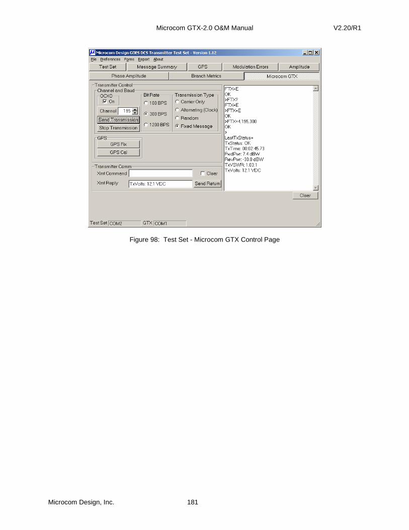
Microcom GTX-2.0 O&M Manual V2.20/R1
Microcom Design, Inc. 181
Figure 98: Test Set - Microcom GTX Control Page

Microcom GTX-2.0 O&M Manual V2.20/R1
Microcom Design, Inc. 182
Appendix A: Command Summary by Function
This appendix provides a command summary in tabular form sorted by functionality.
GOES Transmission Configuration Commands
Command Description CMD Access Section Notes Platform ID PID dtx 11.2.1 aka, NESDIS ID GTX Operation Mode GTX dtx 11.2.2 GOES, METEOSAT, INSAT, etc. Timed Transmit Channel TCH dtx 11.2.3 Timed Tx channel and data rate Timed Transmit Interval TTI dtx 11.2.4 In dd:hh:mm:ss First Transmission Time FTT dtx 11.2.5 As hh:mm:ss Timed Window Length TWL dtx 11.2.6 In seconds, 5-240 Timed Operation Flags TOF dtx 11.2.7 Bit Mapped Value Timed Preamble TPR dtx 11.2.8 Short or Long for 100 bps Timed Data Format TDF dtx 11.2.9 ASCII, Pseudo-Binary, or Binary Timed Data Source TDS dtx 11.2.10 RS-232 or Sensor Timed Data Order TDO dtx 11.2.11 Newest or Oldest Random Transmit Channel RCH dtx 11.2.12 Random channel and data rate Random Transmit Interval RIN dtx 11.2.13 In minutes Randomization Percent RPC dtx 11.2.14 In percent Random Repeat Count RRC dtx 11.2.15 Transmissions per Sequence Random Data Format RDF dtx 11.2.16 ASCII, Pseudo-Binary, or Binary Random Data Source RDS dtx 11.2.17 RS-232 or Sensor Random Data Order RDO dtx 11.2.18 Newest or Oldest Random Operation Flags ROF dtx 11.2.19 Bit Mapped Value
General Transmitter Configuration Commands
Command Description CMD Access Section Notes Transmit Power TXP dtx 11.3.1 In Watts by Mode and bps Time TIM dtx 11.3.2 Manual Time Set Date DAT dtx 11.3.3 Manual Date Set Time Correct TIC all 11.3.4 Manually Re-sync Clock Time Zone Offset TZN dtx 11.3.5 From UTC (in hours, 0.25 resolution) UTC Correction UTC all 11.3.6 Manually Preset UTC Correction Invalid Replace Character IRC dtx 11.3.7 Slash Fill SFL dtx 11.3.8 Use / to Fill Unread Data in Tx Buffers Power Up Enabled PUE dtx 11.3.9 Configure GTX to Power Up Enabled
Transmission Data Storage Commands
Command Description CMD Access Section Notes Timed Data Buffer Load TDT etx 11.4.2 TX must be enabled Timed Buffer Size TBS all 11.4.3 Get Current Size of Timed Tx Buffer Clear Timed Buffer CTB all 11.4.4 Clear the RS-232 Timed Tx Buffer Timed Buffer Dump TBD all 11.4.5 Return Contents of Timed Buffer Random Data Buffer Load RDT etx 11.4.6 TX must be enabled Random Buffer Size RBS all 11.4.7 Get Current Size of Random Tx Buffer Clear Random Buffer CRB all 11.4.8 Clear the RS-232 Timed Tx Buffer Random Buffer Dump RBD all 11.4.9 Return Contents of Timed Buffer Random Buffer Txs Remaining RBT all 11.4.10 Number Remaining in Sequence

Appendix A: Command Summary by Function V2.20/R1
Microcom Design, Inc. 183
Data Collection Setup and Test Commands – SDI-12
Command Description CMD Access Section Notes SDI-12 Sensor Number SSN dtx 11.5.1.1 Set Maximum SDI-12 Sensors (64) SDI-12 Sensor Define SSX dtx 11.5.1.3 X = 0 to 9 (or SSX=nn...) SDI-12 Sensor Label SLX dtx 11.5.1.4 X = 0 to 9 (or SLX=nn...) SDI-12 Sensor Next Sample SMX dtx 11.5.1.5 X = 0 to 9 (or SMX=nn...) SDI-12 Test Command SDI all 11.5.1.6 Supports Pass-Thru Mode SDI-12 Timeout STO all 11.5.1.7
SDI-12 Power Control Commands
Command Description CMD Access Section Notes SDI-12 Power Control SPC all 11.5.2.1 Enable/Disable SDI-12 Buss Power SDI-12 Power Mode SPM dtx 11.5.2.3 Set Default SDI-12 Power Modes SDI-12 Power Table Entry SPX dtx 11.5.2.3 Auto SDI-12 Power On/Off
Data Collection Setup and Test Commands – Internal Sensors
Command Description CMD Access Section Notes Internal Sensor Number ISN dtx 11.5.3.1 Set Maximum Internal Sensors (64) Internal Sensor Define ISX dtx 11.5.3.3 X = 0 to 9 (or ISX=nn…) Internal Sensor Label ILX dtx 11.5.3.4 X = 0 to 9 (or ILX=nn…) Internal Sensor Next Sample IMX dtx 11.5.3.5 X = 0 to 9 (or IMX=nn…) Internal Sensor Test IST all 11.5.3.6 TCXO Temperature TOT All 11.5.3.7 In degrees Celsius Tipping Bucket Count TBC all 11.5.3.8 Raw Counts Tipping Bucket Value TBV all 11.5.3.9 Scaled Value (Counts*Multiplier) Tipping Bucket Multiplier TBM dtx 11.5.3.10 Scaling multiplier Tipping Bucket Rollover TBR dtx 11.5.3.11 Counter rollover limit Tipping Bucket Auto Clear TBA dtx 11.5.3.12 Auto Reset to 0 Daily, Weekly, etc.
Equation Processing Setup/Test Commands
Command Description CMD Access Section Notes Equation Definition EQN dtx 11.6.1 Define/Edit/Delete Equation Equation Test EQT dtx 11.6.2 Verify Equation Syntax Number of Equation Constants EKN dtx 11.6.3.1 Set/Get Maximum Constants (64) Equation Constant Value EKV all 11.6.3.2 Set/Get Equation Constant Value Equation Constant Label EKL dtx 11.6.3.3 Set/Get Equation Constant Label Equation Variable EQV all 11.6.4 Query Equation Variable Value Min, Max, Average Number MMN dtx 11.6.5 Set Maximum MMA Processors (64) Min, Max, Average Definition MMA dtx 11.6.6 Define Min, Max, Average for Sensor
Sensor Data Transmission Setup Commands
Command Description CMD Access Section Notes Timed Parameter Buffer Number TPN dtx 11.7.1 Set Max Timed Data Params (100) Timed Data Param Defintion TDP dtx 11.7.3 Random Param Buffer Number RPN dtx 11.7.2 Set Max Random Data Params (40) Random Data Param Definition RDP dtx 11.7.3 Platform Identification String PIS dtx 11.7.3.1.1 Max 40-Character string Pseudo Binary Character PBX dtx 11.7.3.1.2 X = 1 or 2 Random Trigger Number RTN dtx 11.7.4 Set Maximum Random Triggers (30) Random Report Trigger Definition RRT dtx 11.7.5
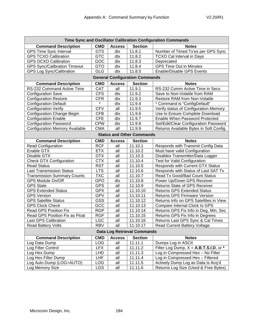
Appendix A: Command Summary by Function V2.20/R1
Microcom Design, Inc. 184
Time Sync and Oscillator Calibration Configuration Commands
Command Description CMD Access Section Notes GPS Time Sync Interval GTS dtx 11.8.1 Number of Timed Tx’es per GPS Sync GPS TCXO Calibration GTC dtx 11.8.2 TCXO Cal Interval in Days GPS OCXO Calibration GOC dtx 11.8.3 Deprecated GPS Sync/Calibration Timeout GTO dtx 11.8.4 GPS Time Out in Minutes GPS Log Sync/Calibration GLG dtx 11.8.5 Enable/Disable GPS Events
General Configuration Commands
Command Description CMD Access Section Notes RS-232 Command Active Time CAT all 11.9.1 RS-232 Comm Active Time in Secs Configuration Save CFS dtx 11.9.2 Save to Non-Volatile from RAM Configuration Restore CFR dtx 11.9.3 Restore RAM from Non-Volatile Configuration Default * dtx 11.9.4 * Command is “ConfigDefault” Configuration Verify CFV all 11.9.5 Verify status of Configuration Memory Configuration Change Begin CFB dtx 11.9.6 Use to Ensure Complete Download Configuration Enable CFE dtx 11.9.7 Enable When Password Protected Configuration Password CPW dtx 11.9.8 Set/Edit/Clear Configuration Password Configuration Memory Available CMA all 11.9.9 Returns Available Bytes in Soft Config
Status and Other Commands
Command Description CMD Access Section Notes Read Configuration RCF all 11.10.1 Responds with Transmit Config Data Enable GTX ETX all 11.10.2 Must have valid Configuration Disable GTX DTX all 11.10.3 Disables Transmitter/Data Logger Check GTX Configuration CTX all 11.10.4 Test for Valid Configuration Read Status RST all 11.10.5 Responds with Current GTX Status Last Transmission Status LTS all 11.10.6 Responds with Status of Last SAT Tx Transmission Summary Counts TXC all 11.10.7 Read Tx Good/Bad Count Status GPS Module On/Off GPO dtx 11.10.8 Power Up/Down GPS Receiver GPS State GPS all 11.10.9 Returns State of GPS Receiver GPS Extended Status GPX all 11.10.10 Returns GPS Extended Status GPS Version GPV all 11.10.11 Returns GPS Firmware Version GPS Satellite Status GSS all 11.10.12 Returns Info on GPS Satellites in View GPS Clock Check GCC all 11.10.13 Compare Internal Clock to GPS Read GPS Position Fix RGP all 11.10.14 Returns GPS Fix Info in Deg, Min, Sec Read GPS Position Fix as Float RGF all 11.10.15 Returns GPS Fix Info in Degrees Last GPS Calibration LGC all 11.10.16 Returns Last GPS Sync & Cal Times Read Battery Volts RBV all 11.10.17 Read Current Battery Voltage
Data Log Retrieval Commands
Command Description CMD Access Section Notes Log Data Dump LOG all 11.11.1 Dumps Log in ASCII Log Filter Control LFX all 11.11.2 Filter Log Dump, X = A,B,T,S,I,D, or * Log Hex Dump LHD all 11.11.3 Log in Compressed Hex – No Filter Log Hex Filter Dump LHF all 11.11.4 Log in Compressed Hex – Filtered Log Auto Dump (LOG=AUTO) LOG all 11.11.5 Actively Dump Log as Data is Acq’d Log Memory Size LGS all 11.11.6 Returns Log Size (Used & Free Bytes)
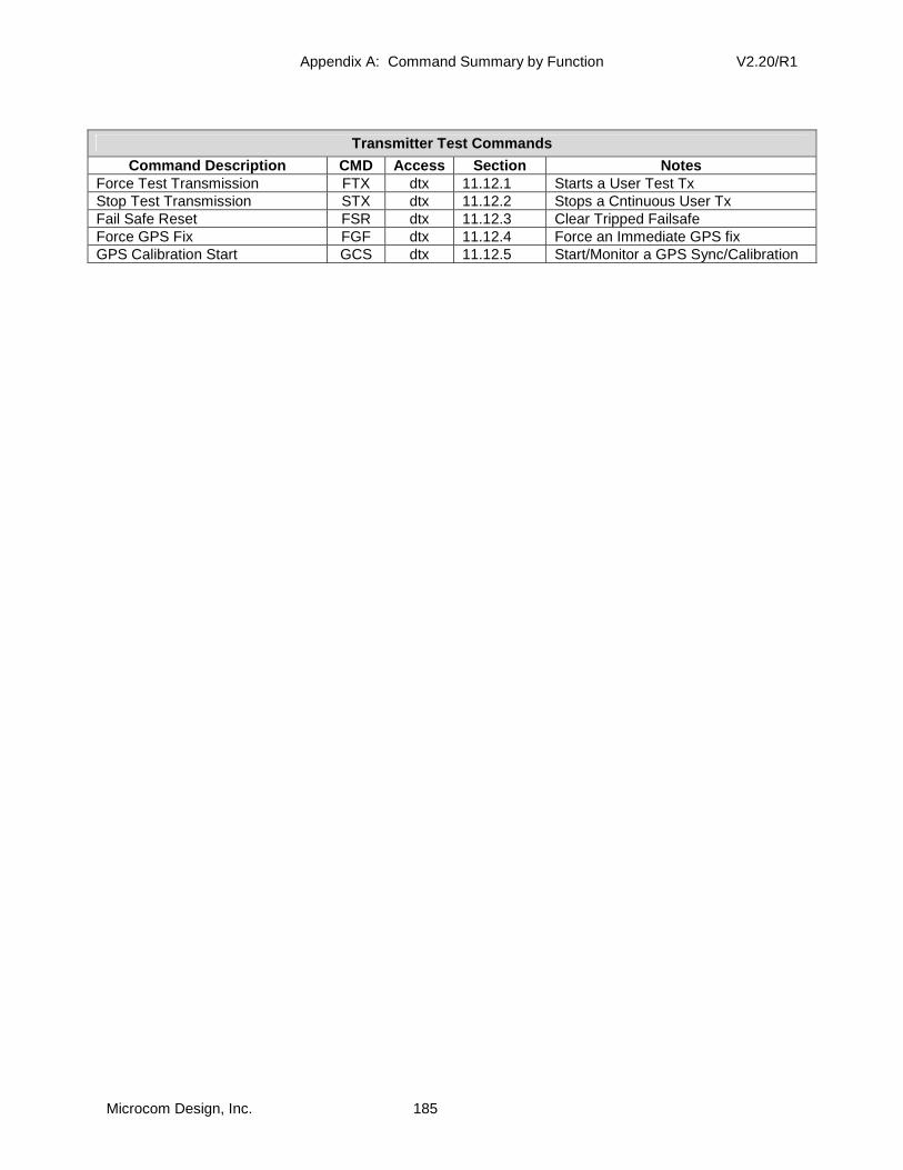
Appendix A: Command Summary by Function V2.20/R1
Microcom Design, Inc. 185
Transmitter Test Commands
Command Description CMD Access Section Notes Force Test Transmission FTX dtx 11.12.1 Starts a User Test Tx Stop Test Transmission STX dtx 11.12.2 Stops a Cntinuous User Tx Fail Safe Reset FSR dtx 11.12.3 Clear Tripped Failsafe Force GPS Fix FGF dtx 11.12.4 Force an Immediate GPS fix GPS Calibration Start GCS dtx 11.12.5 Start/Monitor a GPS Sync/Calibration
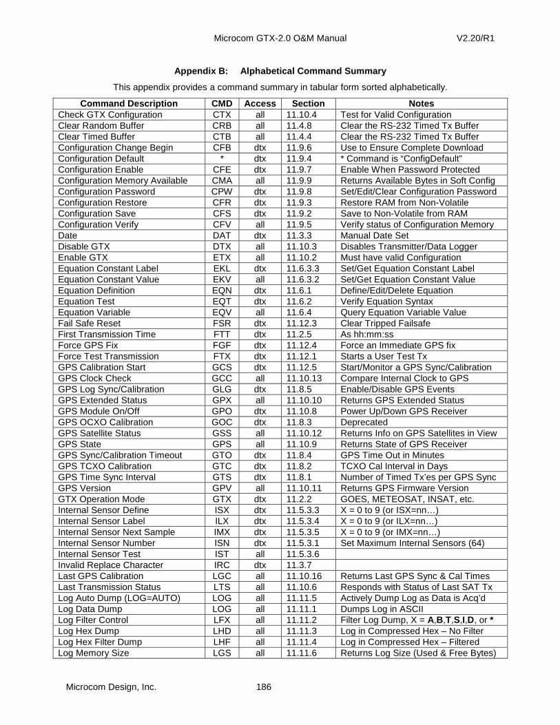
Microcom GTX-2.0 O&M Manual V2.20/R1
Microcom Design, Inc. 186
Appendix B: Alphabetical Command Summary
This appendix provides a command summary in tabular form sorted alphabetically.
Command Description CMD Access Section Notes Check GTX Configuration CTX all 11.10.4 Test for Valid Configuration Clear Random Buffer CRB all 11.4.8 Clear the RS-232 Timed Tx Buffer Clear Timed Buffer CTB all 11.4.4 Clear the RS-232 Timed Tx Buffer Configuration Change Begin CFB dtx 11.9.6 Use to Ensure Complete Download Configuration Default * dtx 11.9.4 * Command is “ConfigDefault” Configuration Enable CFE dtx 11.9.7 Enable When Password Protected Configuration Memory Available CMA all 11.9.9 Returns Available Bytes in Soft Config Configuration Password CPW dtx 11.9.8 Set/Edit/Clear Configuration Password Configuration Restore CFR dtx 11.9.3 Restore RAM from Non-Volatile Configuration Save CFS dtx 11.9.2 Save to Non-Volatile from RAM Configuration Verify CFV all 11.9.5 Verify status of Configuration Memory Date DAT dtx 11.3.3 Manual Date Set Disable GTX DTX all 11.10.3 Disables Transmitter/Data Logger Enable GTX ETX all 11.10.2 Must have valid Configuration Equation Constant Label EKL dtx 11.6.3.3 Set/Get Equation Constant Label Equation Constant Value EKV all 11.6.3.2 Set/Get Equation Constant Value Equation Definition EQN dtx 11.6.1 Define/Edit/Delete Equation Equation Test EQT dtx 11.6.2 Verify Equation Syntax Equation Variable EQV all 11.6.4 Query Equation Variable Value Fail Safe Reset FSR dtx 11.12.3 Clear Tripped Failsafe First Transmission Time FTT dtx 11.2.5 As hh:mm:ss Force GPS Fix FGF dtx 11.12.4 Force an Immediate GPS fix Force Test Transmission FTX dtx 11.12.1 Starts a User Test Tx GPS Calibration Start GCS dtx 11.12.5 Start/Monitor a GPS Sync/Calibration GPS Clock Check GCC all 11.10.13 Compare Internal Clock to GPS GPS Log Sync/Calibration GLG dtx 11.8.5 Enable/Disable GPS Events GPS Extended Status GPX all 11.10.10 Returns GPS Extended Status GPS Module On/Off GPO dtx 11.10.8 Power Up/Down GPS Receiver GPS OCXO Calibration GOC dtx 11.8.3 Deprecated GPS Satellite Status GSS all 11.10.12 Returns Info on GPS Satellites in View GPS State GPS all 11.10.9 Returns State of GPS Receiver GPS Sync/Calibration Timeout GTO dtx 11.8.4 GPS Time Out in Minutes GPS TCXO Calibration GTC dtx 11.8.2 TCXO Cal Interval in Days GPS Time Sync Interval GTS dtx 11.8.1 Number of Timed Tx’es per GPS Sync GPS Version GPV all 11.10.11 Returns GPS Firmware Version GTX Operation Mode GTX dtx 11.2.2 GOES, METEOSAT, INSAT, etc. Internal Sensor Define ISX dtx 11.5.3.3 X = 0 to 9 (or ISX=nn…) Internal Sensor Label ILX dtx 11.5.3.4 X = 0 to 9 (or ILX=nn…) Internal Sensor Next Sample IMX dtx 11.5.3.5 X = 0 to 9 (or IMX=nn…) Internal Sensor Number ISN dtx 11.5.3.1 Set Maximum Internal Sensors (64) Internal Sensor Test IST all 11.5.3.6 Invalid Replace Character IRC dtx 11.3.7 Last GPS Calibration LGC all 11.10.16 Returns Last GPS Sync & Cal Times Last Transmission Status LTS all 11.10.6 Responds with Status of Last SAT Tx Log Auto Dump (LOG=AUTO) LOG all 11.11.5 Actively Dump Log as Data is Acq’d Log Data Dump LOG all 11.11.1 Dumps Log in ASCII Log Filter Control LFX all 11.11.2 Filter Log Dump, X = A,B,T,S,I,D, or * Log Hex Dump LHD all 11.11.3 Log in Compressed Hex – No Filter Log Hex Filter Dump LHF all 11.11.4 Log in Compressed Hex – Filtered Log Memory Size LGS all 11.11.6 Returns Log Size (Used & Free Bytes)
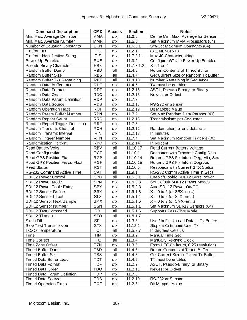
Appendix B: Alphabetical Command Summary V2.20/R1
Microcom Design, Inc. 187
Command Description CMD Access Section Notes Min, Max, Average Definition MMA dtx 11.6.6 Define Min, Max, Average for Sensor Min, Max, Average Number MMN dtx 11.6.5 Set Maximum MMA Processors (64) Number of Equation Constants EKN dtx 11.6.3.1 Set/Get Maximum Constants (64) Platform ID PID dtx 11.2.1 aka, NESDIS ID Platform Identification String PIS dtx 11.7.3.1.1 Max 40-Character string Power Up Enabled PUE dtx 11.3.9 Configure GTX to Power Up Enabled Pseudo Binary Character PBX dtx 11.7.3.1.2 X = 1 or 2 Random Buffer Dump RBD all 11.4.9 Return Contents of Timed Buffer Random Buffer Size RBS all 11.4.7 Get Current Size of Random Tx Buffer Random Buffer Txs Remaining RBT all 11.4.10 Number Remaining in Sequence Random Data Buffer Load RDT etx 11.4.6 TX must be enabled Random Data Format RDF dtx 11.2.16 ASCII, Pseudo-Binary, or Binary Random Data Order RDO dtx 11.2.18 Newest or Oldest Random Data Param Definition RDP dtx 11.7.3 Random Data Source RDS dtx 11.2.17 RS-232 or Sensor Random Operation Flags ROF dtx 11.2.19 Bit Mapped Value Random Param Buffer Number RPN dtx 11.7.2 Set Max Random Data Params (40) Random Repeat Count RRC dtx 11.2.15 Transmissions per Sequence Random Report Trigger Definition RRT dtx 11.7.5 Random Transmit Channel RCH dtx 11.2.12 Random channel and data rate Random Transmit Interval RIN dtx 11.2.13 In minutes Random Trigger Number RTN dtx 11.7.4 Set Maximum Random Triggers (30) Randomization Percent RPC dtx 11.2.14 In percent Read Battery Volts RBV all 11.10.17 Read Current Battery Voltage Read Configuration RCF all 11.10.1 Responds with Transmit Config Data Read GPS Position Fix RGP all 11.10.14 Returns GPS Fix Info in Deg, Min, Sec Read GPS Position Fix as Float RGF all 11.10.15 Returns GPS Fix Info in Degrees Read Status RST all 11.10.5 Responds with Current GTX Status RS-232 Command Active Time CAT all 11.9.1 RS-232 Comm Active Time in Secs SDI-12 Power Control SPC all 11.5.2.1 Enable/Disable SDI-12 Buss Power SDI-12 Power Mode SPM dtx 11.5.2.3 Set Default SDI-12 Power Modes SDI-12 Power Table Entry SPX dtx 11.5.2.3 Auto SDI-12 Power On/Off SDI-12 Sensor Define SSX dtx 11.5.1.3 X = 0 to 9 (or SSX=nn...) SDI-12 Sensor Label SLX dtx 11.5.1.4 X = 0 to 9 (or SLX=nn...) SDI-12 Sensor Next Sample SMX dtx 11.5.1.5 X = 0 to 9 (or SMX=nn...) SDI-12 Sensor Number SSN dtx 11.5.1.1 Set Maximum SDI-12 Sensors (64) SDI-12 Test Command SDI all 11.5.1.6 Supports Pass-Thru Mode SDI-12 Timeout STO all 11.5.1.7 Slash Fill SFL dtx 11.3.8 Use / to Fill Unread Data in Tx Buffers Stop Test Transmission STX dtx 11.12.2 Stops a Cntinuous User Tx TCXO Temperature TOT all 11.5.3.7 In degrees Celsius Time TIM dtx 11.3.2 Manual Time Set Time Correct TIC all 11.3.4 Manually Re-sync Clock Time Zone Offset TZN dtx 11.3.5 From UTC (in hours, 0.25 resolution) Timed Buffer Dump TBD all 11.4.5 Return Contents of Timed Buffer Timed Buffer Size TBS all 11.4.3 Get Current Size of Timed Tx Buffer Timed Data Buffer Load TDT etx 11.4.2 TX must be enabled Timed Data Format TDF dtx 11.2.9 ASCII, Pseudo-Binary, or Binary Timed Data Order TDO dtx 11.2.11 Newest or Oldest Timed Data Param Defintion TDP dtx 11.7.3 Timed Data Source TDS dtx 11.2.10 RS-232 or Sensor Timed Operation Flags TOF dtx 11.2.7 Bit Mapped Value
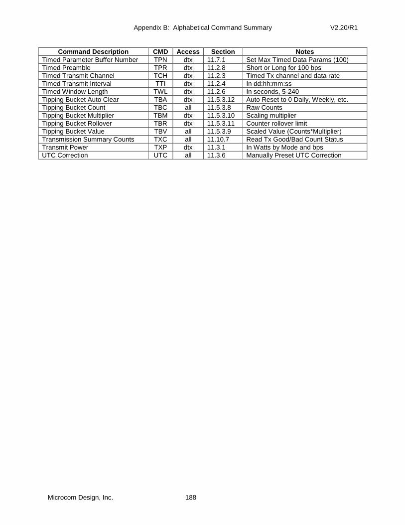
Appendix B: Alphabetical Command Summary V2.20/R1
Microcom Design, Inc. 188
Command Description CMD Access Section Notes Timed Parameter Buffer Number TPN dtx 11.7.1 Set Max Timed Data Params (100) Timed Preamble TPR dtx 11.2.8 Short or Long for 100 bps Timed Transmit Channel TCH dtx 11.2.3 Timed Tx channel and data rate Timed Transmit Interval TTI dtx 11.2.4 In dd:hh:mm:ss Timed Window Length TWL dtx 11.2.6 In seconds, 5-240 Tipping Bucket Auto Clear TBA dtx 11.5.3.12 Auto Reset to 0 Daily, Weekly, etc. Tipping Bucket Count TBC all 11.5.3.8 Raw Counts Tipping Bucket Multiplier TBM dtx 11.5.3.10 Scaling multiplier Tipping Bucket Rollover TBR dtx 11.5.3.11 Counter rollover limit Tipping Bucket Value TBV all 11.5.3.9 Scaled Value (Counts*Multiplier) Transmission Summary Counts TXC all 11.10.7 Read Tx Good/Bad Count Status Transmit Power TXP dtx 11.3.1 In Watts by Mode and bps UTC Correction UTC all 11.3.6 Manually Preset UTC Correction
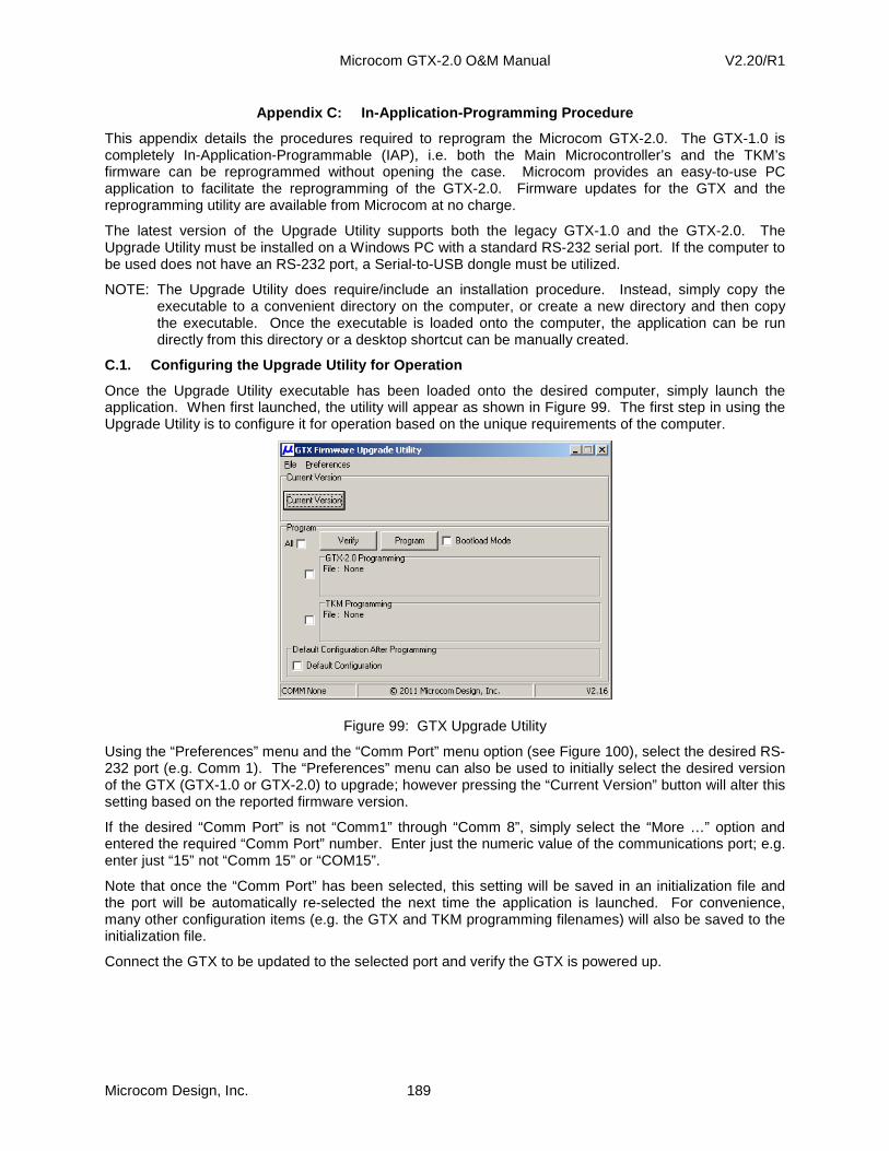
Microcom GTX-2.0 O&M Manual V2.20/R1
Microcom Design, Inc. 189
Appendix C: In-Application-Programming Procedure
This appendix details the procedures required to reprogram the Microcom GTX-2.0. The GTX-1.0 is completely In-Application-Programmable (IAP), i.e. both the Main Microcontroller’s and the TKM’s firmware can be reprogrammed without opening the case. Microcom provides an easy-to-use PC application to facilitate the reprogramming of the GTX-2.0. Firmware updates for the GTX and the reprogramming utility are available from Microcom at no charge.
The latest version of the Upgrade Utility supports both the legacy GTX-1.0 and the GTX-2.0. The Upgrade Utility must be installed on a Windows PC with a standard RS-232 serial port. If the computer to be used does not have an RS-232 port, a Serial-to-USB dongle must be utilized.
NOTE: The Upgrade Utility does require/include an installation procedure. Instead, simply copy the executable to a convenient directory on the computer, or create a new directory and then copy the executable. Once the executable is loaded onto the computer, the application can be run directly from this directory or a desktop shortcut can be manually created.
C.1. Configuring the Upgrade Utility for Operation
Once the Upgrade Utility executable has been loaded onto the desired computer, simply launch the application. When first launched, the utility will appear as shown in Figure 99. The first step in using the Upgrade Utility is to configure it for operation based on the unique requirements of the computer.
Figure 99: GTX Upgrade Utility
Using the “Preferences” menu and the “Comm Port” menu option (see Figure 100), select the desired RS-232 port (e.g. Comm 1). The “Preferences” menu can also be used to initially select the desired version of the GTX (GTX-1.0 or GTX-2.0) to upgrade; however pressing the “Current Version” button will alter this setting based on the reported firmware version.
If the desired “Comm Port” is not “Comm1” through “Comm 8”, simply select the “More …” option and entered the required “Comm Port” number. Enter just the numeric value of the communications port; e.g. enter just “15” not “Comm 15” or “COM15”.
Note that once the “Comm Port” has been selected, this setting will be saved in an initialization file and the port will be automatically re-selected the next time the application is launched. For convenience, many other configuration items (e.g. the GTX and TKM programming filenames) will also be saved to the initialization file.
Connect the GTX to be updated to the selected port and verify the GTX is powered up.
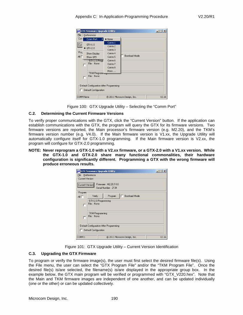
Appendix C: In-Application-Programming Procedure V2.20/R1
Microcom Design, Inc. 190
Figure 100: GTX Upgrade Utility – Selecting the “Comm Port”
C.2. Determining the Current Firmware Versions
To verify proper communications with the GTX, click the “Current Version” button. If the application can establish communications with the GTX, the program will query the GTX for its firmware versions. Two firmware versions are reported, the Main processor’s firmware version (e.g. M2.20), and the TKM’s firmware version number (e.g. V4.0). If the Main firmware version is V1.xx, the Upgrade Utility will automatically configure itself for GTX-1.0 programming. If the Main firmware version is V2.xx, the program will configure for GTX-2.0 programming.
NOTE: Never reprogram a GTX-1.0 with a V2.xx firmwa re, or a GTX-2.0 with a V1.xx version. While the GTX-1.0 and GTX-2.0 share many functional commo nalities, their hardware configuration is significantly different. Programm ing a GTX with the wrong firmware will produce erroneous results.
Figure 101: GTX Upgrade Utility – Current Version Identification
C.3. Upgrading the GTX Firmware
To program or verify the firmware image(s), the user must first select the desired firmware file(s). Using the File menu, the user can select the “GTX Program File” and/or the “TKM Program File”. Once the desired file(s) is/are selected, the filename(s) is/are displayed in the appropriate group box. In the example below, the GTX main program will be verified or programmed with “GTX_V220.hex”. Note that the Main and TKM firmware images are independent of one another, and can be updated individually (one or the other) or can be updated collectively.
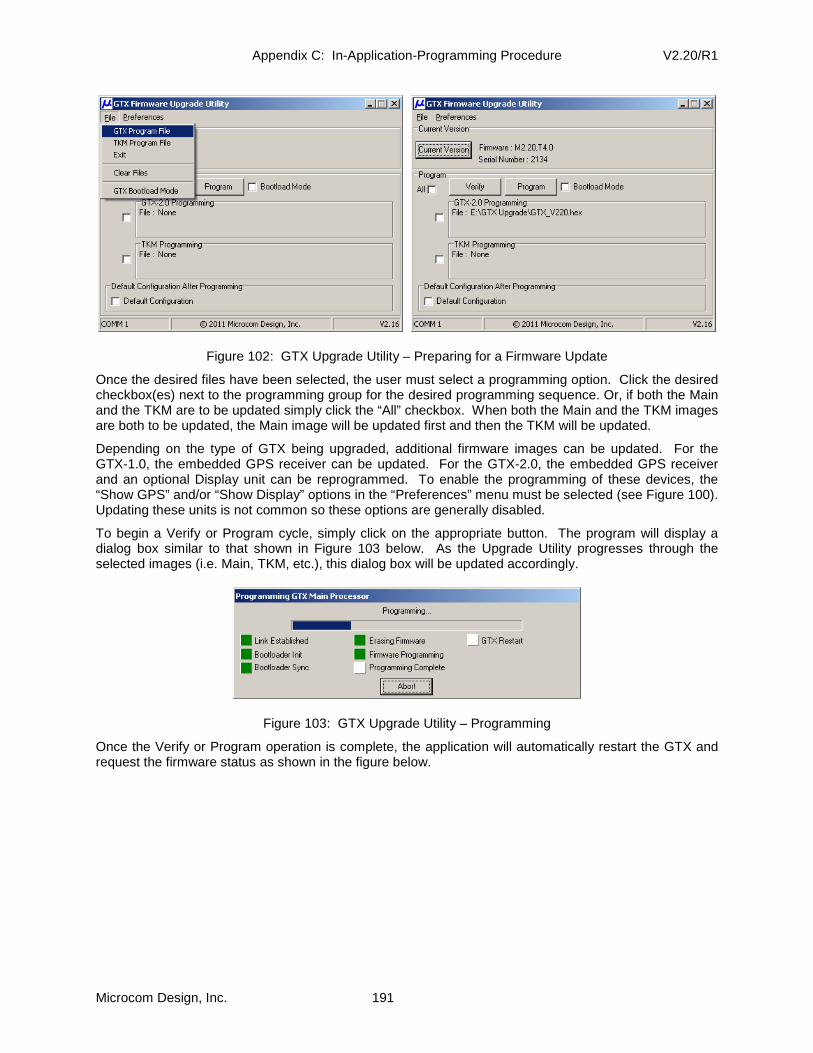
Appendix C: In-Application-Programming Procedure V2.20/R1
Microcom Design, Inc. 191
Figure 102: GTX Upgrade Utility – Preparing for a Firmware Update
Once the desired files have been selected, the user must select a programming option. Click the desired checkbox(es) next to the programming group for the desired programming sequence. Or, if both the Main and the TKM are to be updated simply click the “All” checkbox. When both the Main and the TKM images are both to be updated, the Main image will be updated first and then the TKM will be updated.
Depending on the type of GTX being upgraded, additional firmware images can be updated. For the GTX-1.0, the embedded GPS receiver can be updated. For the GTX-2.0, the embedded GPS receiver and an optional Display unit can be reprogrammed. To enable the programming of these devices, the “Show GPS” and/or “Show Display” options in the “Preferences” menu must be selected (see Figure 100). Updating these units is not common so these options are generally disabled.
To begin a Verify or Program cycle, simply click on the appropriate button. The program will display a dialog box similar to that shown in Figure 103 below. As the Upgrade Utility progresses through the selected images (i.e. Main, TKM, etc.), this dialog box will be updated accordingly.
Figure 103: GTX Upgrade Utility – Programming
Once the Verify or Program operation is complete, the application will automatically restart the GTX and request the firmware status as shown in the figure below.

Appendix C: In-Application-Programming Procedure V2.20/R1
Microcom Design, Inc. 192
Figure 104: GTX Upgrade Utility – Programming Complete

Microcom GTX-2.0 O&M Manual V2.20/R1
Microcom Design, Inc. 193
Appendix D: Antenna Pointing Curves
The curves of Figure 105 and Figure 106 are included to allow quick determination of the elevation and azimuth angles to GOES East and GOES West, respectively. Both spacecraft are in equatorial, geosynchronous orbit with GOES East at 75W degrees (-75 degrees) and GOES West at 135W degrees (-135 degrees).
In each figure, the closed (red) curves labeled with the bold numbers give the elevation angle, and the black curves give the azimuth relative to true north. The curves are labeled in 10 degree increments, which is adequate for pointing the low gain antennas (less than 11 dB) used in conjunction with DCS transmitters. Each of the four major quadrants is labeled as N, S, E, and W to indicate the direction pointing to the spacecraft. In Figure 106, the longitude scale is from –225 to –45 degrees. Normally, the range from –225 and –180 degrees would be expressed as 135E to 180E. To correct longitudes expressed as East, subtract 360 degrees from the longitude, i.e. 155E corresponds to –215 degrees.
As an example, the NOAA Command and Data Acquisition Station (CDA) located at Wallops Island is located at 38N and 75.5W. By convention for latitude, N is positive and S is negative; and for longitude E is positive and W is negative. From Figure 105, the azimuth and elevation angles from WCDA are 179 and 46 degrees, respectively. WCDA is only 0.5 degrees west of GOES East. Similarly, from Figure 106, the azimuth and elevation to GOES West are 245 and 15 degrees, respectively.
Note that the azimuth angles are relative to true north and must be corrected for the local magnetic declination. For WCDA, this correction is 11.5W. A west correction is added to the true north azimuth, while an east correction is subtracted. Thus, the magnetic azimuths to GOES East and West from WCDA are 191 and 257 degrees, respectively.
Outside the 0 degree elevation curve, the azimuths are meaningless since the spacecraft is below the local horizon. In fact, the GOES DCS system is intended for use above a 5-degree elevation angle. Below this elevation, the wide antenna beams are strongly impacted by reflection from the earth, making the path loss unpredictable.
As explained in Section 12.1.6, the GTX Utility also includes a function to determine the antenna azimuth and elevation angles for a specific location provided in latitude and longitude.
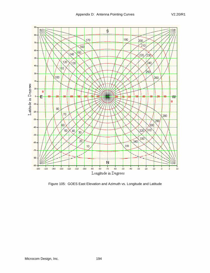
Appendix D: Antenna Pointing Curves V2.20/R1
Microcom Design, Inc. 194
Figure 105: GOES East Elevation and Azimuth vs. Longitude and Latitude

Appendix D: Antenna Pointing Curves V2.20/R1
Microcom Design, Inc. 195
Figure 106: GOES West Elevation and Azimuth vs. Longitude and Latitude

Microcom GTX-2.0 O&M Manual V2.20/R1
Microcom Design, Inc. 196
Appendix E: List of Acronyms
8PSK 8 State Phase Shift Keying AC Alternating Current
AGC Automatic Gain Control
AM Amplitude Modulation
ANSI American National Standards Institute ARM Abnormal Response Messages ASCII American Standard Code for Information Interchange BCH Bose, Chaudhari and Hocquenghem BER Bit Error Rate, Bit Errors Received bps, BPS Bits per Second BPSK Binary Phase Shift Keying CDA Command and Data Acquisition CGMS Coordination Group for Meteorological Satellites DADDS DCS Administrative and Data Distribution System DAMS-NT Data Acquisition and Monitoring System – New Technology DAPS Data Collection System Automated Processing System dB Decibel dBm Decibels relative to one milliwatt DC Direct Current DCP Data Collection Platform DCPRS Data Collection Platform Radio Set DCS Data Collection System Demod Demodulator DOMSAT Domestic Satellite DPCM Dual Pilot Control Module DRGS Direct Readout Ground Station DSP Digital Signal Processor; Digital Signal Processing EIRP Equivalent Isotropic Radiated Power EOT, ETX End of Transmission FSS Frame Synch Sequence GOES Geostationary Operational Environmental Satellite GUI Graphical User Interface HRIT High Rate Information Transmission Hz Hertz ICD Interface Control Document I/O Input/Output IF Intermediate Frequency IIM Input Interface Module (DAMS-NT) IP Internet Protocol IRIG-B Inter-Range Instrumentation Group code B for 1 second timing standard

Appendix E: List of Acronyms V2.20/R1
Microcom Design, Inc. 197
kHz Kilohertz L-band 1694.3 to 1694.7 MHz for this DCS application LAN Local Area Network LRGS Local Readout Ground Station LRIT Low Rate Information Transmission LSB Least Significant Bit max Maximum MHz Megahertz min Minimum MSB Most Significant Bit NESDIS National Environmental Satellite, Data, and Information Service NIC Network Interface Controller or Network Interface Card NIC-MUX Network Interface Controller and Multiplexer (DAMS-NT) NOAA National Oceanic and Atmospheric Administration NRZ-L Non-Return to Zero - Level NSOF NOAA’s Satellite Operations Facility NWS National Weather Service NWSTG National Weather Service Telecommunications Gateway O&M Operations and Maintenance OEM Original Equipment Manufacturer OS Operating System PM Phase Modulation ppm, PPM parts per million PSK Phase Shift Keying QMB Quad Mother Board (DAMS-NT) RF Radio Frequency sps Symbols per Second sync Synchronizer; Synchronization TCP Transfer Control Protocol U.S. United States UHF Ultra High Frequency (401.7 to 402.1 MHz for this DCS application) UTC V Volts VC Virtual Channel Vpp Volts peak-to-peak WCDA Wallops Command and Data Acquisition WCDAS Wallops Command and Data Acquisition Station
Microcom GTX-2.0 O&M Manual V2.20/R1
Microcom Design, Inc. 198
Appendix F: Web References
GOES DCS Description
http://www.osd.noaa.gov/daps/pdocs.htm
see “Other Attachments”
goesdes.pdf and ngop1.pdf
GOES HDR Certification
http://www.osd.noaa.gov/download/index.htm
GOES DCS Home Page
http://noaasis.noaa.gov/DCS
GOES DCS Adminstration and Data Dessimination Syste m (DADDS)
Wallops
https://dcs1.noaa.gov
https://dcs2.noaa.gov
NSOF
https://dcs3.noaa.gov
https://dcs4.noaa.gov