Microeconomics

James B. Wilcox

Resources provided by:

The University of Southern MississippiCenter for Economic and Entrepreneurship Education,

Mississippi State University, & Virtual Economics

Economics…is the study of how individuals and society choose, with or without the use of money, to employ scarce productive resources to produce various commodities over time and distribute them for consumption, now and in the future, among various people and groups in a society.

The Economic Way of Thinking:Three Activities to Demonstrate Marginal Analysis 2

5

9

12

14

15

15

14

2

3

4

3

2

1

0

-1

MTE Microeconomics

© 2009 South-Western/Cengage Learning

99

Production and Costs

• Producers: Maximize profit• Opportunity cost

– All resources have an opportunity cost

• Explicit costs– Payments for resources

• Implicit costs – Opportunity cost of resources owned by

the firm / firm owners

– No cash payment

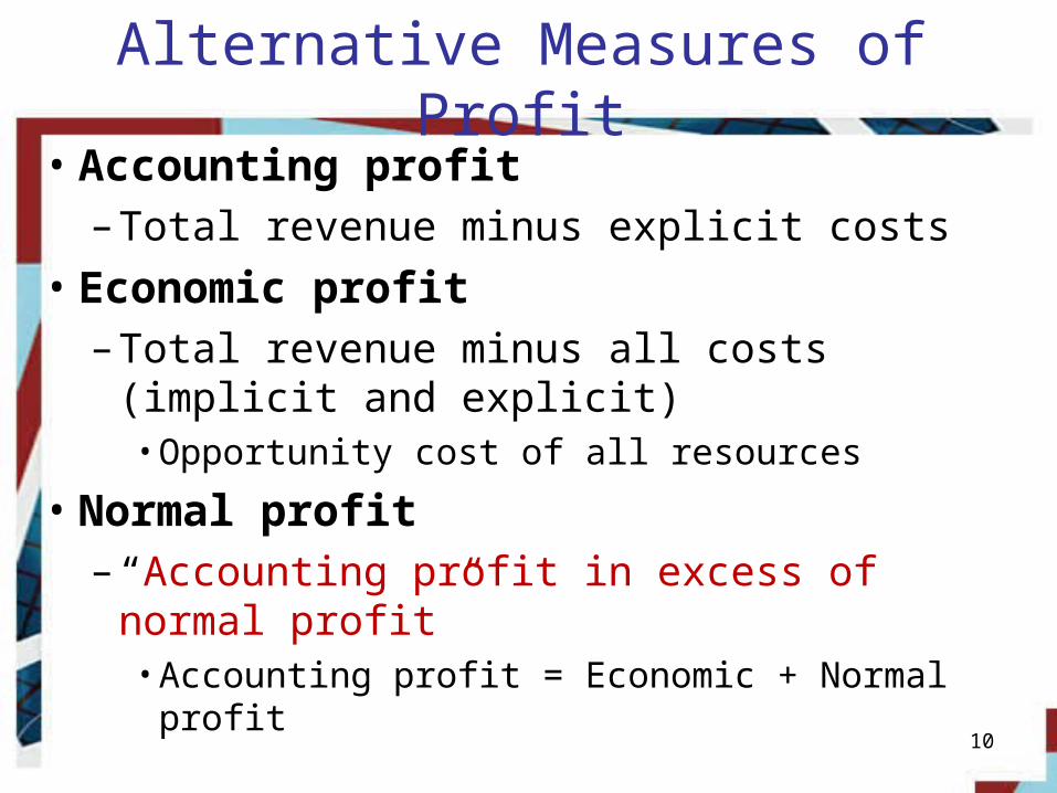
Alternative Measures of Profit

• Accounting profit– Total revenue minus explicit costs

• Economic profit– Total revenue minus all costs (implicit and

explicit)• Opportunity cost of all resources

• Normal profit– “Accounting profit in excess of normal profit”

• Accounting profit = Economic + Normal profit10

Production in the Short Run

• Variable resources– Can be varied quickly

• Fixed resources – Cannot be altered easily

• Short run– At least one resource is fixed

• Long run – No resource is fixed

11

Law of Diminishing Marginal Returns

• Total product: total output produced • Production function

– Relationship between amount of resources employed and total product

• Marginal product: the change in total product resulting from a one-unit increase in a resource employed by the firm

12

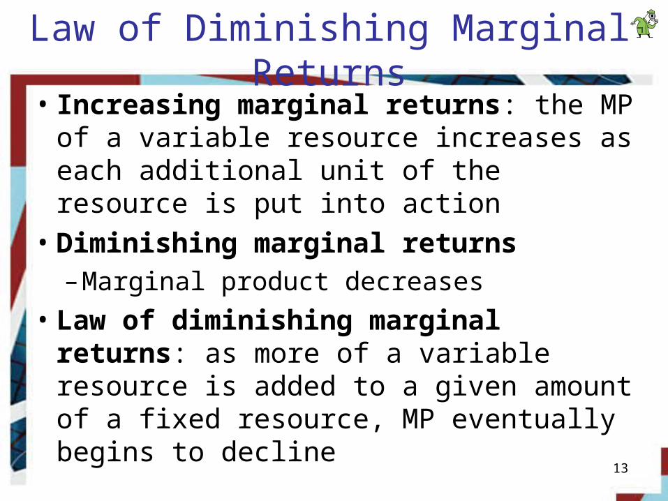
Law of Diminishing Marginal Returns

• Increasing marginal returns: the MP of a variable resource increases as each additional unit of the resource is put into action

• Diminishing marginal returns – Marginal product decreases

• Law of diminishing marginal returns: as more of a variable resource is added to a given amount of a fixed resource, MP eventually begins to decline 13

Exhibit 3The total and marginal product of labor

14

5

10

15

Tot

al p

rodu

ct

(to

ns/d

ay)

5 10 Workers per day0

5 10 Workers per day

1

3

5

Mar

gina

l pro

duct

(to

ns/d

ay)

0

2

4

Total

product

Marginal product

Negative

marginal

returns

Diminishing but

positive

marginal returns

Increasing

marginal

returns

(a) Total product

(b) Marginal product

Costs in the Short Run

• Fixed cost (TFC): any production costs that a firm incurs even when it is not producing output; Ex: overhead—rent, insurance, property taxes

• Variable cost (TVC) any production costs that change as output changes; TVC = 0 when the firm is not producing any output; Ex.: labor costs

15

Costs in the Short Run

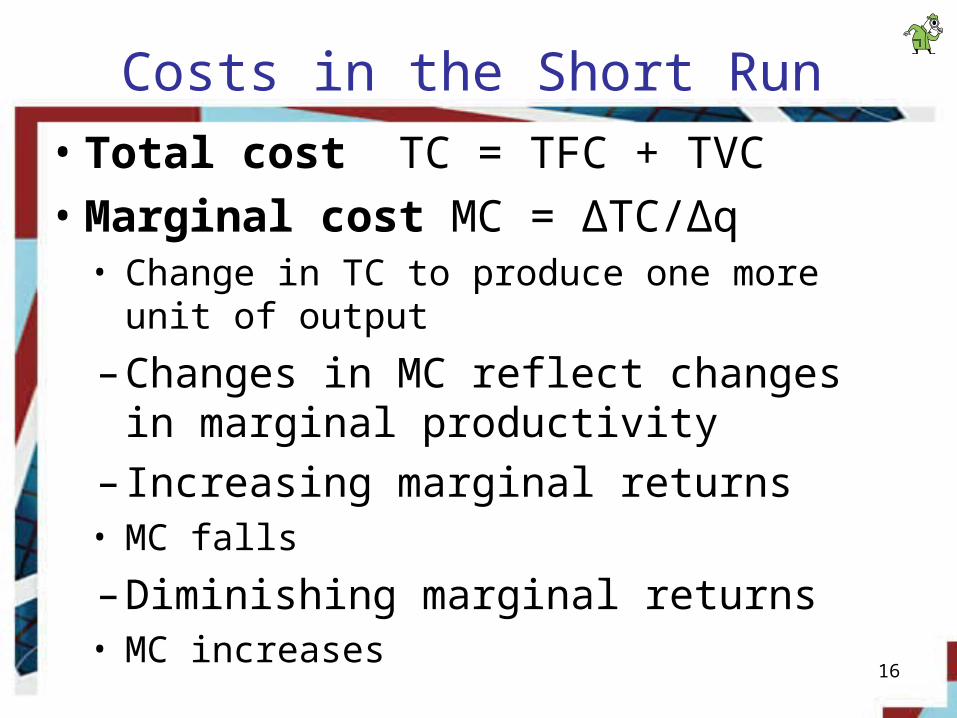
• Total cost TC = TFC + TVC• Marginal cost MC = ∆TC/∆q

• Change in TC to produce one more unit of output

– Changes in MC reflect changes in marginal productivity

– Increasing marginal returns• MC falls

– Diminishing marginal returns• MC increases 16

Exhibit 4Short-run TC and MC data for Smoother Mover

17

(1)Tons moved

per day(q)

(2)Fixed cost(FC)

(3)Workers per day

(4)Variable

cost(VC)

(5)Total cost

(TC=FC+VC)

(6)Marginal cost

MC=∆TC/∆q

0259

121415

$200 200 200 200 200 200 200

0123456

$0100200300400500600

18

(1)Tons moved

per day(q)

(2)Fixed cost(FC)

(3)Workers per day

(4)Variable

cost(VC)

(5)Total cost

(TC=FC+VC)

(6)Marginal cost

MC=∆TC/∆q

0259

121415

$200 200 200 200 200 200 200

0123456

$0100200300400500600

$200 300 400 500 600 700 800

-$50.00 33.33 25.00 33.33 50.55 100.00

•SR TC and MC data for Smoother Mover

Exhibit 5TC and MC curves for Smoother Mover

19

200

$500

Tot

al d

olla

rs

25

Cos

t per

ton

$50Marginal cost

9 15 Tons per day0 63 12

Fixed cost

Total cost

Tons per day0 9 1563 12

Variable costFixed

cost

FC = $200 at all levels of output

VC starts from origin; increases slowly at first;

with diminishing returns, VC increases rapidly

TC is the vertical sum of FC and VC

MC first declines: increasing marginal returns;

then increases: diminishing marginal returns

Average Cost in the Short Run

• Average variable cost AVC = VC/q• Average total cost ATC = TC/q• When MC < average cost

– The marginal pulls down the average

• When MC > average cost– The marginal pulls up the average

• U-shape of average cost curves– Law of diminishing marginal returns

20

Exhibit 7Average and marginal cost curves; Smoother Movers

21

0 5 10 15 Tons per day

$150

125

100

75

50

25

Cos

t pe

r to

n

ATC

AVC

MC

ATC and AVC: decline,

reach low points, then rise.

When MC is below AVC (ATC),

AVC (ATC) is falling

When MC = AVC (ATC), AVC (ATC) is at its minimum.

When MC is above AVC (ATC),

AVC (ATC) is increasing.

Perfect Competition

© 2009 South-Western/ Cengage Learning

2323

What is Market Structure?

• Market structure– Number of suppliers

– Product’s degree of uniformity

– Ease of entry into the market

– Forms of competition among forms

• Industry– All firms supplying output to a market

Types of Market Structure

• Perfect Competition: many sellers; horizontal demand curve

• Monopoly: one seller• Monopolistic Competition: many

sellers; downward-sloping demand curve• Oligopoly: few sellers

24

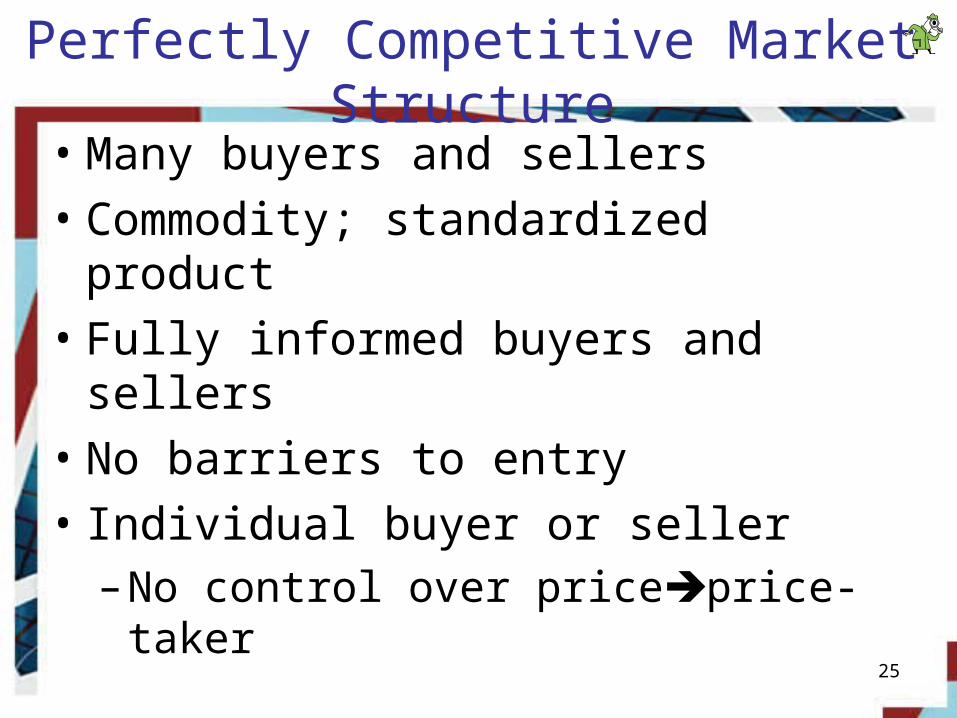
Perfectly Competitive Market Structure

• Many buyers and sellers• Commodity; standardized product• Fully informed buyers and sellers• No barriers to entry• Individual buyer or seller

– No control over priceprice-taker

25

Demand Under Perfect Competition

• Market price– Determined by market demand and

supply. All firms must use this price on their products.

• Demand curve facing one supplier– Horizontal line at the market price

– Perfectly elastic

26

Short Run Profit Maximization

• Maximize economic profit– Choose the quantity at which total

revenue (TR) exceeds total cost (TC) by the greatest amount

– TR = PxQ

• Profit = TR – TC

27

Golden Rule of Profit Maximization

• Marginal revenue: the change in TR from selling an additional unit– ∆TR/∆q

• MR = P = AR (perfect competition)• Golden rule: produce where MR = MC

– Expand output: MR>MC

– Stop before MC>MR

28

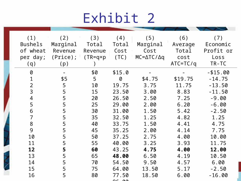
Exhibit 2

• Short-run cost and revenue; perfectly competitive firm

29

(1)Bushels of wheat

per day;(q)

(2)MarginalRevenue

(Price); (p)

(3)Total

Revenue(TR=q×p)

(4)TotalCost(TC)

(5)Marginal

CostMC=∆TC/∆q

(6)Average

Total costATC=TC/q

(7)Economic

Profit or LossTR-TC

0123456789

10111213141516

-$5555555555555555

$05

101520253035404550556065707580

$15.0019.7523.5026.5029.0031.0032.5033.7535.2537.2540.0043.2548.0054.5064.0077.5096.00

-$4.753.753.002.502.001.501.251.502.002.753.254.756.509.50

13.5018.50

-$19.7511.758.837.256.205.424.824.414.144.003.934.004.194.575.176.00

-$15.00-14.75-13.50-11.50-9.00-6.00-2.501.254.757.75

10.0011.7512.0010.506.00-2.50-16.00

Monopoly

© 2009 South-Western/ Cengage Learning

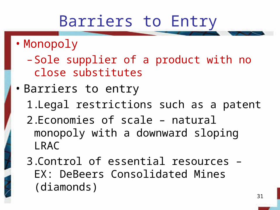
Barriers to Entry

• Monopoly– Sole supplier of a product with no close

substitutes

• Barriers to entry1.Legal restrictions such as a patent

2.Economies of scale – natural monopoly with a downward sloping LRAC

3.Control of essential resources – EX: DeBeers Consolidated Mines (diamonds)

31

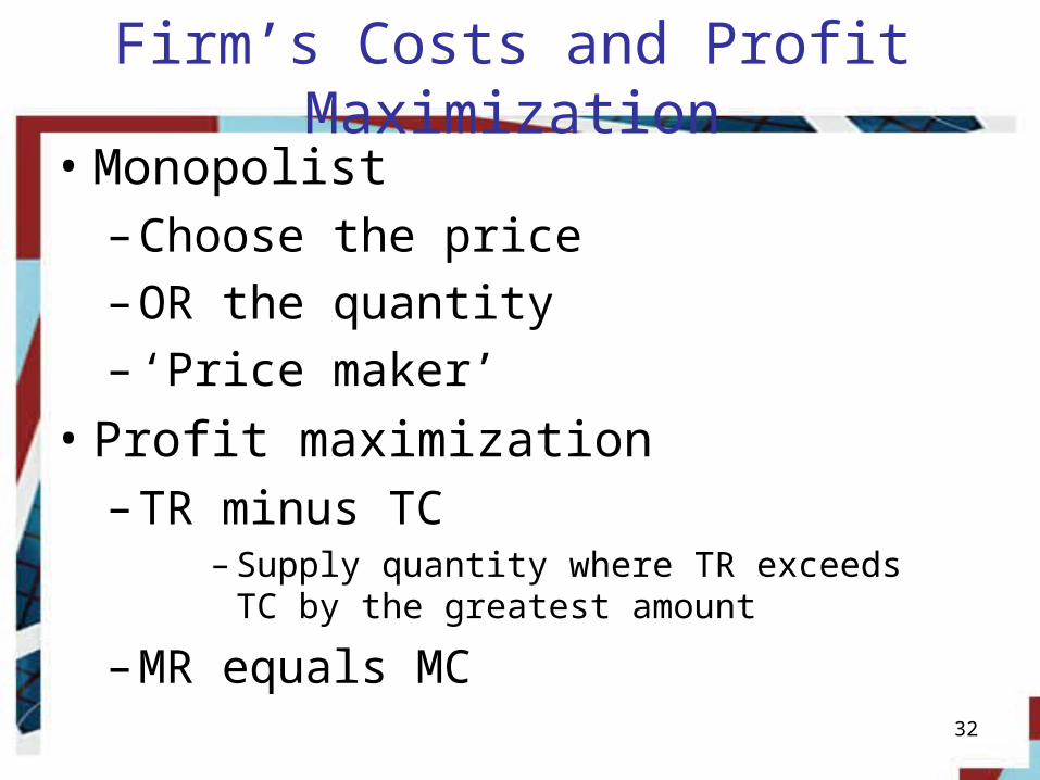
Firm’s Costs and Profit Maximization

• Monopolist– Choose the price

– OR the quantity

– ‘Price maker’

• Profit maximization– TR minus TC

– Supply quantity where TR exceeds TC by the greatest amount

– MR equals MC32

Exhibit 5

• Short-run costs and revenue for a monopolist

33

(1)Diamonds

per day(Q)

(2)Price(AR)(p)

(3)Total

RevenueTR=p×Q

(4)Marginal Revenue

MR=∆TR/∆Q

(5)TotalCost(TC)

(6)Marginal

Cost(MC)

(7)Average

Total costATC=TC/q

(8)Total profit

or loss(=TR-TC)

0123456789

1011121314151617

$7,7507,5007,2507,0006,7506,5006,2506,0005,7505,5005,2505,0004,7504,5004,2504,0003,7503,500

0$7,50014,50021,00027,00032,50037,50042,00046,00049,50052,50055,00057,00058,50059,50060,00060,00059,500

-$7,5007,0006,5006,0005,5005,0004,5004,0003,5003,0002,5002,0001,5001,000500

0-500

$15,00019,75023,50026,50029,00031,00032,50033,75035,25037,25040,00043,25048,00054,50064,00077,50096,000121,000

-$4,7503,7503,0002,5002,0001,5001,2501,5002,0002,7503,2504,7506,5009,500

13,50018,50025,000

-$19,75011,7508,8337,7506,2005,4204,8204,4104,1404,0003,9304,0004,1904,5705,1706,0007,120

-$15,000-12,250-9,000-5,500-2,0001,5005,0008,25010,75012,25012,50011,7509,0004,000-4,500-17,500-36,000-61,500

Monopolistic Competition

and Oligopoly

Monopolistic Competition

• Characteristics– Many producers

– Low barriers to entry

– Slightly different products• A firm that raises prices: lose some

customers to rivals

– Some control over price ‘Price makers’• Downward sloping D curve

– Act independently35

Monopolistic Competition

• Product differentiation– Physical differences

• Appearance; quality

– Location• Spatial differentiation

– Services

– Product image• Promotion; advertising

36

Oligopoly

• Few sellers• Barriers to entry

– Economies of scale

– Legal restrictions

– Brand names

– Control over an essential resource

– High cost of entry• Start-up costs; advertising

• Crowding out the competition37

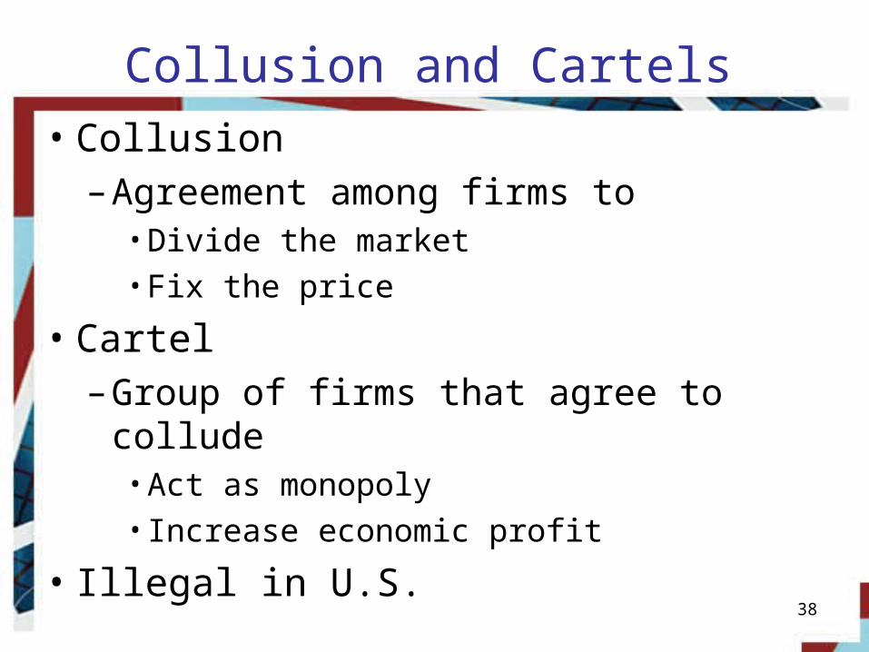
Collusion and Cartels

• Collusion– Agreement among firms to

• Divide the market• Fix the price

• Cartel– Group of firms that agree to collude

• Act as monopoly• Increase economic profit

• Illegal in U.S.38

Comparisons Across Market Structures

CharacteristicsPerfect Competition

Monopolistic Competition

Oligopoly Monopoly

Sellers Many Many Few One

Products Identical Close substitutes, but not identical

Identical (ex: oil) ORDifferent (ex: cereal)

No close substitutes

Prices Price-taker Price-maker Price-maker Price-maker

Entry and Exit No barriers No barriers Barriers Barriers

Demand horizontal Downward-sloping

Downward-sloping

Downward-sloping

Profits MR=MC MR=MC MR=MC MR=MC

Long-Run Economic Profits

Zero Zero Greater than zero

Greater than zero

39

Public Goods

and Public Choice

© 2009 South-Western/ Cengage Learning

Characteristics of Pure Public Goods

• Nonrival: more than one person can consume the good or service at the same timeMC of an additional user is zero

• Nonexcludable: difficult or impossible to exclude others from deriving the benefits of the public good

41

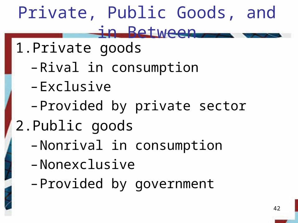
Private, Public Goods, and in Between

1. Private goods– Rival in consumption

– Exclusive

– Provided by private sector

2. Public goods– Nonrival in consumption

– Nonexclusive

– Provided by government

42

Private, Public Goods, and in Between

3. Natural monopoly– Nonrival but exclusive

– With congestion: private goods

– Provided by private sector or government

4. Open-access good– Rival but nonexclusive

– Regulated by government

43

Exhibit 1

• Categories of goods

44

Paying for Public Goods

• Tax = marginal valuation– Free-rider problem

• People try to benefit from the public goods without paying for them

– Ability to pay

45

Externalities

and the Environment

© 2009 South-Western/ Cengage Learning

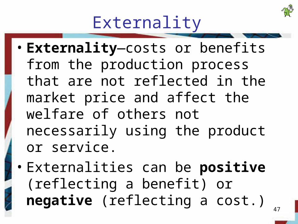
Externality

• Externality—costs or benefits from the production process that are not reflected in the market price and affect the welfare of others not necessarily using the product or service.

• Externalities can be positive (reflecting a benefit) or negative (reflecting a cost.)

47

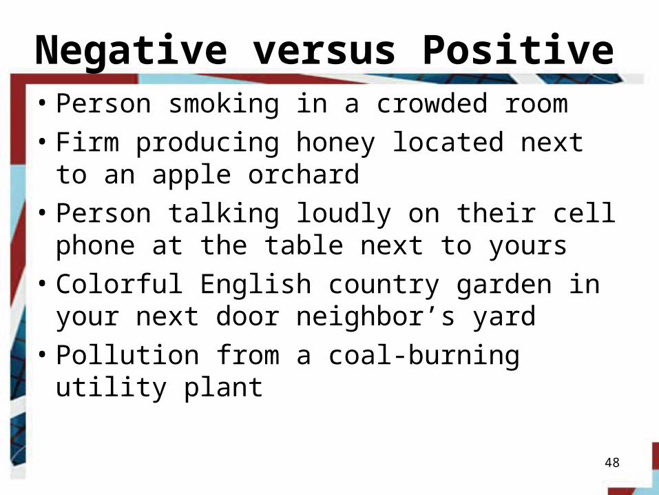
Negative versus Positive• Person smoking in a crowded room• Firm producing honey located next to an

apple orchard• Person talking loudly on their cell phone

at the table next to yours• Colorful English country garden in your

next door neighbor’s yard• Pollution from a coal-burning utility plant

48

Negative Externality

• Marginal Private Cost (MPC): private costs of production such as wages, costs of materials, rent, insurance, taxes, etc.

• Marginal External Cost (MEC): valuation of marginal damage caused by negative externality

• Marginal Social Cost (MSC):

= MPC + MEC

49

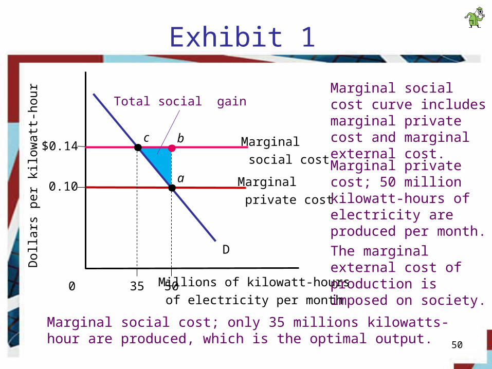
Exhibit 1

50

0.10

$0.14

Dol

lars

per

kilo

wat

t-ho

ur

Marginal

social cost Marginal private cost; 50 million kilowatt-hours of electricity are produced per month.

The marginal external cost of production is imposed on society.

350 Millions of kilowatt-hours

of electricity per month50

Marginal

private cost

D

a

c

Marginal social cost; only 35 millions kilowatts-hour are produced, which is the optimal output.

Marginal social cost curve includes marginal private cost and marginal external cost.

Total social gain

b

Public Responses to Negative Externalities

• Tax the polluter: levy a tax on each level of output produced by the polluter in an amount equal to the MEC inflicted at the socially efficient level of output.

• Subsidize the polluter: pay the polluter not to pollute

• Environmental regulation: Government tells the polluter to reduce pollution or face sanctions (1990 Clean Air Act)

51

Public Responses to Negative Externalities

• Economic efficiency approach: marketable permits—government sells producers permits to pollute (pollution rights)

52

Positive Externality

• Marginal Private Benefit (MPB): private benefits of production or consumption

• Marginal External Benefit (MEB): valuation of marginal benefit created by positive externality

• Marginal social benefit = MPB + MEB

53

Positive Externalities

• Beneficial externalities• Education

– Personal benefits

– Benefits to society• Positive externality

• Public policy– To increase quantity beyond private

optimum

54

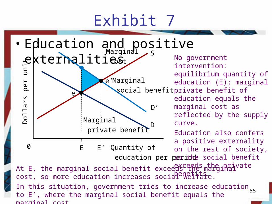
Exhibit 7

• Education and positive externalities

55

E0 E’ Quantity of

education per period

Dol

lars

per

uni

t

DMarginal

private benefit

D’

Marginal

social benefit

SMarginal

cost

e’

e

No government intervention: equilibrium quantity of education (E); marginal private benefit of education equals the marginal cost as reflected by the supply curve.

Education also confers a positive externality on the rest of society, so the social benefit exceeds the private benefits.

At E, the marginal social benefit exceeds the marginal cost, so more education increases social welfare.

In this situation, government tries to increase education to E’, where the marginal social benefit equals the marginal cost.

Income Distribution

and Poverty

© 2009 South-Western/ Cengage Learning

Income Distribution by Quintiles

• Distribution of income– U.S. households

– Ranked by income

– Five groups of equal size (quintiles)

• Percentage of income received in 1970– Poorest 20% of population

• 4.1% of income

– Richest 20% of population• 43.3% of income

57

Exhibit 1

• Share of aggregate household income by quintile: 1970, 1980, 1990, and 2005

58

Income Distribution by Quintiles

• Richest 20% of population– Increased share of income

– Two-earner households

• Poorest 20% of population– Decreased share of income

– Single-parent household

59

The Lorenz Curve

• Lorenz curve: graphical representation of the size of the income distribution

• The diagonal line represents equal distribution or perfect income equality. Each 20 percent of the population receives 20 percent of total income.

60

Exhibit 2: Lorenz Curve

61

Households (cumulative percent)

Inco

me

(cum

ulat

ive

perc

ent)

1970

2005

a

bEqual d

istrib

ution

Lorenz curve: convenient way of showing the % of total income received by any given % of households when households are arrayed from smallest to largest.

Point a: in 1970, the bottom 80% of households received 56.7% of all income.

Point b: in 2005, the share of all income going to the bottom 80% of households was lower than in 1970.

If income were evenly distributed across households, the Lorenz curve would be a straight line.

Why Incomes Differ

• Number of household members working• Education, ability, job experience• Productivity• High-income household

• Well-educated couple; both spouses employed

• Low-income household• One person living alone• Single-parent, female• Poorly educated

62

A College Education Pays More

• Median wage, past 20 years– Only high-school diploma: decreased 6%

• Industry deregulation; declining unionization• Information technology

– College degree: increased 12%• Information technology• Higher rewards for education

63

Redistribution Programs

• Official U.S. poverty level– Family of four: $19,971 in 2005

– $13.70 per person per day

– Pretax money income– Includes cash transfers– Excludes value of non-cash transfers

» Food stamps; Medicaid; Subsidized housing» Employer-provided health insurance

– Recessions: Increase in poverty

• International poverty line: • $1 per person per day 64

Exhibit 3 (1959-2005)

• Number and percentage of US population in poverty

65

Social Insurance

1. Social security

2. Medicare

3. Unemployment insurance

4. Workers’ compensation• Deducted from workers’ pay

– Aimed at people with work history

• Income redistribution • From rich to poor • From young to old 66

Income Assistance

• Welfare programs• Means-tested program: only individuals

with incomes below a certain level qualify

1.Cash transfers programs– Temporary assistance for needy families:

TANF replaced AFDC

– Supplemental security income

– General assistance aid

– Earned-income tax credit67

Income Assistance

2. In-kind transfer programs– Medicaid: basic medical care for the poor

– Food stamps

– Housing assistance

– Support for day care, school lunches

– Energy assistance

– Education and training

68

Percent of population living in poverty by state

69

Welfare Reform

• Welfare-to-work programs• 1997: Temporary assistance for needy

families– States: more control

• Maximum time to receive benefits: 5 years• Work participation rates: must work after 2

years of receiving benefits• Benefit levels are reduced less than dollar

for dollar when one obtains a job

70

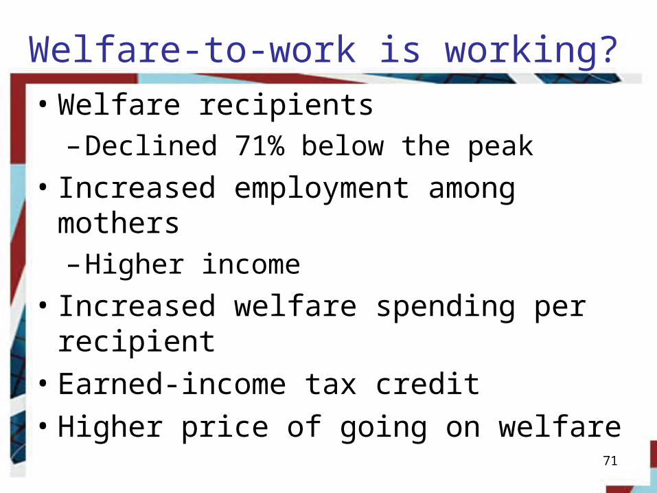
Welfare-to-work is working?

• Welfare recipients– Declined 71% below the peak

• Increased employment among mothers – Higher income

• Increased welfare spending per recipient• Earned-income tax credit• Higher price of going on welfare

71

QuickTime™ and aTIFF (Uncompressed) decompressor

are needed to see this picture.

Statistics from U.S. GAO

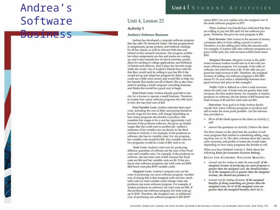
Andrea’s SoftwareBusiness

73

74

$60

$60

$60

$60

$60

$60

$60

$60

$145

$180

$210

$245

$285

$330

$385

$525

$35

$30

$35

$40

$45

$55

$65

$112

$168

$224

$56

$56

$56

$56

$56

$56

$56

$280

$336

$392

$448

$560

$56

$56

$56

$56

$56

$56

$56

-$49 (loss)-$33 (loss)

$14 (profit)

$35 (profit)

$62 (profit)

$63 (profit)

$54 (profit)

$35 (profit)

Microeconomics

James B. Wilcox

Resources provided by:

The University of Southern MississippiCenter for Economic and Entrepreneurship Education,

Mississippi State University, & Virtual Economics