micromechanical study of pfz in aluminum alloys1017317/fulltext01.pdf · grain boundaries. pfz has...

IN DEGREE PROJECT SOLID MECHANICS,SECOND CYCLE, 30 CREDITS

, STOCKHOLM SWEDEN 2016

Micromechanical study of PFZ in aluminum alloys

HOSSEIN SHARIATI

KTH ROYAL INSTITUTE OF TECHNOLOGYSCHOOL OF ENGINEERING SCIENCES

www.kth.se

Royal Institute of Technology

School of Engineering Sciences

Micromechanical Study of PFZ in

Aluminum Alloys

Hossein Shariati

Master degree project in Solid Mechanics

Supervisor: Jonas Faleskog

Stockholm, Sweden, June 2016

i

Summary

There are a number of experiments showing that the ductility of aluminum alloys decreases

during age-hardening heat treatment. Observing the grains of age-hardened aluminum alloys

at the micron scale, one can notice that there are precipitate-free zones (PFZs) along the

grain boundaries. PFZ has yield stress three times lower than the grain interior (bulk) due to

absence of alloying elements. As a result, PFZ is suspected to be the reason for ductility

reduction of alloys. On the other hand, a number of experiments performed on specimens

with micron-scale dimensions have shown that the plastic deformation of crystalline

materials is size-dependent. These micron-scale dimensions which can influence the

mechanical behavior, such as yield stress or hardening, are not taken into account in the

conventional plasticity theory, therefore another theory has been developed. That theory is

Strain Gradient Plasticity (SGP). The specific SGP theory used here is a so called ‘higher-

order theory’ in the sense that higher order stresses as well as additional boundary conditions

are included in the theory. SGP theory also includes length scale parameters in order to be

dimensionally consistent.

On a recent study conducted by Fourmeau et al. (Fourmeau, 2015), transmission electron

microscopy (TEM) is used to display the geometrical properties and the chemical

composition of PFZ in the AA7075-T651 aluminum alloy. It is observed that the width of PFZ

is about 20 to 40 nm. In the present thesis, the properties for PFZ and bulk material provided

by that study are used for a micromechanical finite element model of a microstructure

including the bulk, PFZ and the grain boundary (GB). A uniaxial loading condition is applied

to the representative volume element (RVE) and SGP theory is hired in order to capture the

plastic strain fields as well as the stress triaxiality in PFZ and bulk region. Moreover a

damage criterion is employed and studied for models with PFZ and without PFZ to

understand the role of PFZ in reduction of the ductility of aluminum alloys. It is found that

the damage parameter is much higher in the presence of PFZ. Finally, the void growth is

studied by adding voids at critical locations to the model.

Keywords: precipitate-free zones; micromechanics, strain gradient plasticity;

ii

Sammanfattning

Det finns ett flertal experiment som visar att duktiliteten hos aluminiumlegeringar minskar under åldringshärdning. Vid observationer på mikronivå av korn i en åldringshärdad aluminiumlegering kan ’precipitate-free zones’ (PFZs) iakttas längs korngränserna. På grund av avsaknaden av legeringsämnen har dessa zoner en sträckgräns som är tre gånger lägre än kornets inre del (bulkmaterial). Förekomsten av PFZ misstänkt därför ligga till grund för minskningen av duktilitet hos dessa legeringar. Å andra sidan har experiment som utförts på provstavar med dimensioner i storleksordningen mikrometer visat att plastisk deformation av kristallina material är storleksberoende. Dessa längskaleeffekter, vilka kan influera det mekaniska beteendet såsom sträckgräns och hårdnande, tas inte i beaktning i konventionell plasticitetsteori och det har därför utvecklats en ny teori, ’Strain Gradient Plasticity’ (SGP). Den SGP-teori som används i detta arbete är av typen ’högre ordningens teori’, vilket innebär att högre ordningens spänningar samt ytterligare randvillkor är inkluderade i teorin. SGP-teorin inkluderar även längdskalningsparametrar för att behålla konsekventa dimensioner.

I en nyligen utförd studie av Fourmeau et al. (Formeau, 2015) användes transmissionselektronmikroskopi (TEM) för att ta fram de geometriska egenskaperna och den kemiska kompositionen av PFZ i aluminiumlegeringen AA7075-T651. I studien framgår att bredden av PFZ är omkring 20 till 40 nm. I detta examensarbete används de erhållna egenskaperna hos PFZ och ”bulkmaterialet” i en mikromekanisk finita element modell av en mikrostruktur inkluderande ”bulkmaterial”, PFZ och korngränser. En enaxlig last appliceras på ett representativ volym element (RVE) och SGP-teorin utnyttjas för att ta fram det plastiska töjningsfältet samt det treaxliga spänningstillståndet i PFZ och bulk regionen. Dessutom introduceras ett skadekriterium för modeller med och utan PFZ för att få en förståelse för hur PFZ inverkar på minskningen av duktilitet hos aluminiumlegeringar. Studien visar att skadeparametern har ett högre värde i modeller med PFZ. Slutligen undersöks hålrumstillväxten genom att addera hålrum vid kritiska positioner i modellen.

Nyckelord: precipitate-free zones, mikromekanik, strain gradient plasticity;

iii

Acknowledgement

The work presented in this thesis is done between January and June 2016 at the department

of Solid Mechanics, Royal Institute of Technology in Stockholm, Sweden. First of all, I would

like to express my gratitude to my supervisor Prof. Jonas Faleskog, for giving me the

opportunity to work on this interesting project. Secondly, I would like to thank Dr. Carl

Dahlberg, who helped me a lot during this work. I have also enjoyed several discussions with

PhD student Mohammadali Asgharzadeh.

Stockholm, June 2016

Hossein Shariati

iv

Contents

Summary ......................................................................................................................................................... i

Sammanfattning ............................................................................................................................................. ii

Acknowledgement ......................................................................................................................................... iii

1 Introduction ............................................................................................................................................ 1

1.1 Literature study ............................................................................................................................. 1

1.2 Purpose .......................................................................................................................................... 2

2 Theory ..................................................................................................................................................... 3

2.1 Interface ......................................................................................................................................... 3

2.2 Strain gradient plasticity (SGP) .................................................................................................... 3

2.3 Damage parameter ........................................................................................................................ 7

3 Model ...................................................................................................................................................... 9

3.1 Material properties ........................................................................................................................ 9

3.2 Micromechanical model ................................................................................................................ 9

3.3 Mesh generation .......................................................................................................................... 10

3.4 Boundary conditions ................................................................................................................... 15

3.5 Solution ........................................................................................................................................ 16

3.6 Post-processing ........................................................................................................................... 16

4 Results and discussion .........................................................................................................................20

4.1 Parametric study .........................................................................................................................20

4.2 Models with and without PFZ ..................................................................................................... 32

4.3 Models with voids ........................................................................................................................ 36

4.4 PFZ width investigation .............................................................................................................. 39

5 Conclusion ............................................................................................................................................ 42

6 References ............................................................................................................................................. 43

7 Appendix ............................................................................................................................................... 44

Introduction

1

1 Introduction

The aluminum alloy considered in this thesis is AA7075 (7xxx) which is a high-strength alloy

often used for industrial purposes. It can be hardened as a result of precipitation hardening

(age hardening) process. Precipitation hardening is related to increased strength due to the

presence of small finely dispersed second phase particles, commonly called precipitates

within the original phase matrix. In spite of high strength properties of 7xxx series, these

series of alloys are suspected to loss of other properties such as ductility. Ductility is the

deformation capacity of a material after yielding, or its ability to dissipate energy during the

plastic deformation. The loss of ductility is known to be due to precipitate free zones (PFZ) in

the vicinity of the grain boundaries (GB) within the microstructure of alloy. In fact PFZ

material is softer as it has a lower yield stress compared to the grain interior (bulk) due to

absence of alloying elements. The width and properties of PFZ is a result of different items

such as ageing temperature and time. As a result of different properties of PFZ material

compared to bulk material, the plastic flow is nonhomogeneous and there is plastic flow

localization which leads to fracture.

The plastic deformation of crystalline materials, such as aluminum, is size-dependent.

However, size effects are not accounted for in conventional plasticity. Therefore the Strain

Gradient Plasticity (SGP) was developed. By using SGP theory, we can enter length scale

parameters to the material constitutive law. As an example the grain size in aluminum is

considered as a length scale that affects material parameters such as yield stress and power

law hardening moduli. SGP is a higher order theory in the sense that higher order stresses

and extra boundary conditions are included in the theory. Moreover, SGP theory can be

understood by dislocation theory which explains the hardening phenomena in materials as a

result of the accumulation of both statistically stored dislocations (SSD) and geometrically

necessary dislocations (GND). The gradient in plastic strain is proportional to the density of

the geometrically necessary dislocations. Tension and torsion of thin copper wires confirm

the material hardening due to plastic strain gradient.

1.1 Literature study

Trying to understand the PFZ influence on mechanical properties of aluminum alloys, a lot of

investigations are conducted in the literature. In one of those studies (Srivatsan et al., 1991),

Srivatsan and Lavernia investigate the influence of PFZ along grain boundaries on

mechanical properties for an aluminum alloy. They conclude that the ductility decreases due

to the restriction of plastic deformation in PFZ along grain boundaries and fracture happens

when a critical local strain is reached in PFZ. In another study (Ludtka et al., 1982), Ludtka

and Laughlin investigate the effects of microstructure and strength on the fracture toughness

of ultra-high strength aluminum alloys. They suggeste that different strength between the

matrix and PFZ is the reason to the fracture toughness behavior of the alloys. Moreover, in

(Pardoen et al., 2003) the competition between intergranular and transgranular failure is

qualitatively studied. The PFZ has a lower yield stress, therefore it starts to deform plastically

and the grain interior only deforms elastically at this step. The elastic region imposes a strong

constraint on PFZ, resulting in high stress triaxiality in PFZ. As a result, the void growth rate

is accelerated in PFZ and consequently there will be a rapid coalescence of the voids. Then

the bulk material starts to yield and the stress triaxiality drops in PFZ. Due to higher

hardening of PFZ, a higher constraint is now applied on the grain interior. Therefore, voids

start to grow more rapidly within the grain until they finally coalesce.

Introduction

2

Evaluation of PFZ effects on the macroscopic behavior is very difficult because of numerous

reasons (Fourmeau et al., 2015). Firstly, the material of PFZ is different from the bulk and its

width is about nanometer, it is therefore difficult to find its mechanical properties from

laboratory tests. Macroscopic specimens of temper conditions which are similar to PFZ

material are used to find the PFZ’s mechanical properties. The assumption that the PFZ is a

highly supersaturated solid solution leads to the point that the W temper (solution heat

treated only) should be representative for the PFZ. Secondly, the stress states in the

precipitate-free zone is different from the macroscopic loading condition. As for an example,

in the case of macroscopic uniaxial load, the stress state in PFZ is not uniaxial and there is a

significant amount of stress triaxiality in PFZ. Moreover, there are several parameters

affecting the macroscopic behavior, e.g. PFZ width, size and spacing of precipitates, yield

stress and work-hardening behavior of PFZ and bulk. As a result of the mentioned

difficulties, it should be noted that the parametric study presented in this thesis is qualitative.

A number of studies performed have shown that plasticity is a size dependent phenomena.

Those studies have concluded that the material response to the loading condition is stronger

for smaller sizes, e.g. fine-grained metals are stronger than coarse-grained ones.

1.2 Purpose

There are a number of numerical simulations in the literature trying to capture the PFZ

influence on mechanical behavior of aluminum alloys. In most of those studies, the

conventional plastic theory are employed to solve the boundary value problem. However, in

the present thesis Strain gradient plasticity (SGP) framework for isotropic materials

(Gudmundson, 2004) is used as a basis for the work.

The objective of this thesis is to numerically model the RVE1 of high strength aluminum alloy,

using the bulk and PFZ features which are observed experimentally in (Fourmeau et al.,

2015). This model is employed to solve boundary value problems using SGP-FEM program

developed by Dahlberg and Faleskog (Dahlberg and Faleskog, 2013; Dahlberg et al., 2013).

Then a parametric study is done to investigate the effect of each parameter on the

macroscopic behavior under a uniaxial loading condition. Finally a damage parameter, which

is a function of the effective plastic strain and stress triaxiality, is engaged and studied for the

model with PFZ and the model without PFZ.

Section 2 describes a brief summary of the theory behind the numerical model. Section 3

presents the micromechanical model of an idealized microstructure, the FEM model and the

MATLAB scripts which are meshing, solving and post-processing the results. Section 4

provides the numerical results and discussion. Section 5 is about the conclusions and future

works.

1 In order to predict the macroscopic behavior of a material, which is non-homogeneous on the microstructural level, a sufficiently large volume must be considered. The volume must be representative of the average material behavior. Such a volume is denoted as a representative volume element (RVE).

Theory

3

2 Theory

2.1 Interface

Heterogeneity of plastic flow in metals is often due to the presence of interfaces. In fact

interfaces act like barriers to dislocation motions. The grain boundary is an example of

interfaces. The boundary between PFZ and bulk region can also be considered as another

example of interfaces as a result of the change of material properties. The interfaces can be

stiff and mostly impenetrable to dislocations or soft and transparent. The main result of the

interaction between dislocation movement and the interfaces is the hardening effect. The

interface effects on plastic flow can be introduced by using strain gradient plasticity models

(SGP).

2.2 Strain gradient plasticity (SGP)

The theory for approaching the problem presented in this report is based on the higher order

strain gradient plasticity theory by Gudmundson (Gudmundson, 2004). Very brief summary

of the theory is presented in this section.

The kinematic relations between primary displacements 𝑢𝑖 and plastic strains 휀𝑖𝑗𝑃 are as

follow

휀𝑖𝑗 =

1

2(𝑢𝑖,𝑗 + 𝑢𝑗,𝑖), (1)

휀𝑖𝑗 = 휀𝑖𝑗𝑒 + 휀𝑖𝑗

𝑝, (2)

휀𝑘𝑘𝑝= 0, (3)

where 휀𝑖𝑗𝑒 is the elastic strain. Equation (3) is due to incompressibility in continuum plasticity.

Following the idea in (Fleck et al., 2009), new relations are introduced as

휀�̂�𝑗 =

1

2(휀𝑖𝑗

𝑝2+ 휀𝑖𝑗

𝑝1), (4)

휀�̌�𝑗 = 휀𝑖𝑗𝑝2− 휀𝑖𝑗

𝑝1 , (5)

where the first relation describes the average plastic strain across an interface and the second

equation is showing the difference between plastic stains at an interface. The advantage of

using these relations is that we can have discontinuous plastic strain fields.

In the SGP theory used in this work, contributions of the work performed by plastic strains

휀𝑖𝑗𝑃 and their gradients 휀𝑖𝑗,𝑘

𝑃 in the body Ω and the energy stored in internal interfaces 𝑆𝑖𝑛𝑡 are

added to the conventional virtual work formulation.

∫ [𝜎𝑖𝑗𝛿휀𝑖𝑗 + (𝑞𝑖𝑗 − 𝑠𝑖𝑗)𝛿휀𝑖𝑗

𝑝+𝑚𝑖𝑗𝑘𝛿휀𝑖𝑗,𝑘

𝑝]𝑑𝑉

Ω

+∫ [�̌�𝑖𝑗𝛿휀�̂�𝑗 + �̂�𝑖𝑗𝛿휀�̌�𝑗]𝑑𝑆 𝑆𝑖𝑛𝑡

= ∫ [𝑇𝑖𝛿𝑢𝑖 +𝑀𝑖𝑗𝛿휀𝑖𝑗𝑝]𝑑𝑆

𝑆𝑒𝑥𝑡.

(6)

where the RHS is the work done on the external boundary 𝑆𝑒𝑥𝑡. Here 𝜎𝑖𝑗 is Cauchy stress and

𝑠𝑖𝑗 = 𝜎𝑖𝑗 − 𝛿𝑖𝑗𝜎𝑘𝑘 3⁄ is its deviator. 𝑞𝑖𝑗 and 𝑚𝑖𝑗 are called micro stress and moment stress.

Theory

4

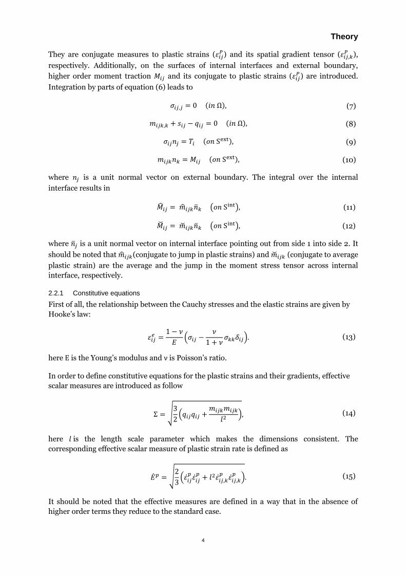
They are conjugate measures to plastic strains (휀𝑖𝑗𝑃 ) and its spatial gradient tensor (휀𝑖𝑗,𝑘

𝑃 ),

respectively. Additionally, on the surfaces of internal interfaces and external boundary,

higher order moment traction 𝑀𝑖𝑗 and its conjugate to plastic strains (휀𝑖𝑗𝑃 ) are introduced.

Integration by parts of equation (6) leads to

𝜎𝑖𝑗,𝑗 = 0 (𝑖𝑛 Ω), (7)

𝑚𝑖𝑗𝑘,𝑘 + 𝑠𝑖𝑗 − 𝑞𝑖𝑗 = 0 (𝑖𝑛 Ω), (8)

𝜎𝑖𝑗𝑛𝑗 = 𝑇𝑖 (𝑜𝑛 Sext), (9)

𝑚𝑖𝑗𝑘𝑛𝑘 = 𝑀𝑖𝑗 (𝑜𝑛 Sext), (10)

where 𝑛𝑗 is a unit normal vector on external boundary. The integral over the internal

interface results in

�̂�𝑖𝑗 = �̂�𝑖𝑗𝑘�̅�𝑘 (𝑜𝑛 Sint), (11)

�̌�𝑖𝑗 = �̌�𝑖𝑗𝑘�̅�𝑘 (𝑜𝑛 Sint), (12)

where �̅�𝑗 is a unit normal vector on internal interface pointing out from side 1 into side 2. It

should be noted that �̂�𝑖𝑗𝑘(conjugate to jump in plastic strains) and �̌�𝑖𝑗𝑘 (conjugate to average

plastic strain) are the average and the jump in the moment stress tensor across internal

interface, respectively.

2.2.1 Constitutive equations

First of all, the relationship between the Cauchy stresses and the elastic strains are given by

Hooke’s law:

휀𝑖𝑗𝑒 =

1 − 𝜈

𝐸(𝜎𝑖𝑗 −

𝜈

1 + 𝜈𝜎𝑘𝑘𝛿𝑖𝑗). (13)

here E is the Young’s modulus and ν is Poisson’s ratio.

In order to define constitutive equations for the plastic strains and their gradients, effective

scalar measures are introduced as follow

Σ = √3

2(𝑞𝑖𝑗𝑞𝑖𝑗 +

𝑚𝑖𝑗𝑘𝑚𝑖𝑗𝑘

𝑙2), (14)

here 𝑙 is the length scale parameter which makes the dimensions consistent. The

corresponding effective scalar measure of plastic strain rate is defined as

�̇�𝑝 = √2

3(휀�̇�𝑗

𝑝휀�̇�𝑗𝑝+ 𝑙2휀�̇�𝑗,𝑘

𝑝휀�̇�𝑗,𝑘𝑝). (15)

It should be noted that the effective measures are defined in a way that in the absence of

higher order terms they reduce to the standard case.

Theory

5

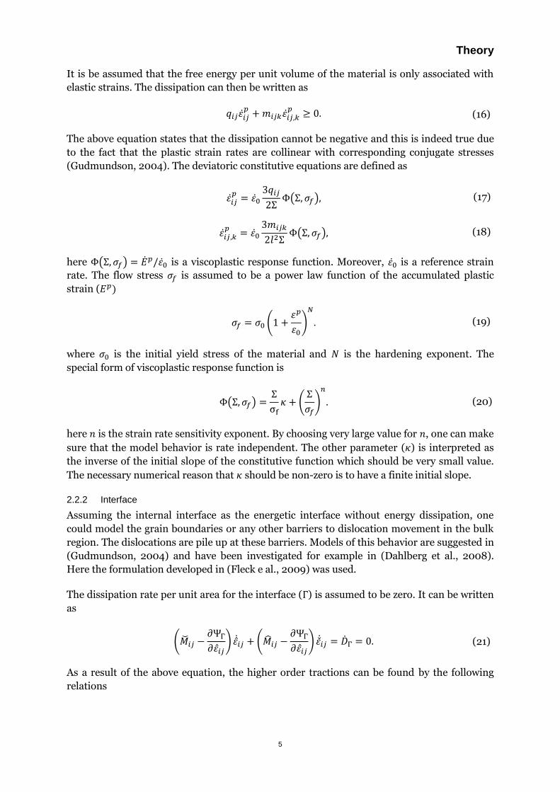
It is be assumed that the free energy per unit volume of the material is only associated with

elastic strains. The dissipation can then be written as

𝑞𝑖𝑗휀�̇�𝑗𝑝+𝑚𝑖𝑗𝑘휀�̇�𝑗,𝑘

𝑝≥ 0. (16)

The above equation states that the dissipation cannot be negative and this is indeed true due

to the fact that the plastic strain rates are collinear with corresponding conjugate stresses

(Gudmundson, 2004). The deviatoric constitutive equations are defined as

휀�̇�𝑗𝑝= 휀0̇

3𝑞𝑖𝑗

2ΣΦ(Σ, 𝜎𝑓), (17)

휀�̇�𝑗,𝑘𝑝

= 휀0̇3𝑚𝑖𝑗𝑘

2𝑙2ΣΦ(Σ, 𝜎𝑓), (18)

here Φ(Σ, 𝜎𝑓) = �̇�𝑝/휀0̇ is a viscoplastic response function. Moreover, 휀0̇ is a reference strain

rate. The flow stress 𝜎𝑓 is assumed to be a power law function of the accumulated plastic

strain (𝐸𝑝)

𝜎𝑓 = 𝜎0 (1 +

휀𝑝

휀0)

𝑁

. (19)

where 𝜎0 is the initial yield stress of the material and 𝑁 is the hardening exponent. The

special form of viscoplastic response function is

Φ(Σ, 𝜎𝑓) =

Σ

σf𝜅 + (

Σ

𝜎𝑓)

𝑛

. (20)

here 𝑛 is the strain rate sensitivity exponent. By choosing very large value for 𝑛, one can make

sure that the model behavior is rate independent. The other parameter (𝜅) is interpreted as

the inverse of the initial slope of the constitutive function which should be very small value.

The necessary numerical reason that 𝜅 should be non-zero is to have a finite initial slope.

2.2.2 Interface

Assuming the internal interface as the energetic interface without energy dissipation, one

could model the grain boundaries or any other barriers to dislocation movement in the bulk

region. The dislocations are pile up at these barriers. Models of this behavior are suggested in

(Gudmundson, 2004) and have been investigated for example in (Dahlberg et al., 2008).

Here the formulation developed in (Fleck e al., 2009) was used.

The dissipation rate per unit area for the interface (Γ) is assumed to be zero. It can be written

as

(�̌�𝑖𝑗 −

𝜕ΨΓ𝜕휀�̂�𝑗

)휀̂�̇�𝑗 + (�̂�𝑖𝑗 −𝜕ΨΓ𝜕휀�̂�𝑗

)휀̌�̇�𝑗 = �̇�Γ = 0. (21)

As a result of the above equation, the higher order tractions can be found by the following

relations

Theory

6

�̌�𝑖𝑗 =


, (22)

�̂�𝑖𝑗 =


, (23)

where ΨΓ is the interface potential function and it depends on the plastic strains at the

internal interface.

ΨΓ = ΨΓ(휀�̂�𝑗 , 휀�̌�𝑗). (24)

It would be useful to introduce the effective measures, the average amount of plastic strains

at interface (휀+) and plastic mismatch (휀−), as follow

휀+ = √휀�̂�𝑗휀�̂�𝑗 , (25)

휀− = √휀�̌�𝑗휀�̌�𝑗 , (26)

and as a result

ΨΓ = ΨΓ(휀+, 휀−), (27)

The differential of potential function becomes

𝑑ΨΓ =

𝜕ΨΓ𝜕휀+

𝑑휀+ +𝜕ΨΓ𝜕휀−

𝑑휀− = �̌�𝑖𝑗𝑑휀�̂�𝑗 + �̂�𝑖𝑗𝑑휀�̌�𝑗 , (28)

which is equivalent to

�̌�𝑖𝑗 =

𝜕ΨΓ𝜕휀+

𝜕휀+

𝜕휀�̂�𝑗+𝜕ΨΓ𝜕휀−

𝜕휀−

𝜕휀�̂�𝑗= 𝜓Γ(휀

+)휀�̂�𝑗

휀+, (29)

�̂�𝑖𝑗 =

𝜕ΨΓ𝜕휀+

𝜕휀+

𝜕휀�̌�𝑗+𝜕ΨΓ𝜕휀−

𝜕휀−

𝜕휀�̌�𝑗= 𝜓Γ(휀

+)휀�̌�𝑗

휀+, (30)

A simple form of 𝜓Γ used here is

𝜓Γ(휀∗) = 𝐺0𝐿

∗휀∗ (31)

where 𝐺0 and 𝐿∗ are interface stiffness and length scales, respectively. The subscript ∗ is

either + or −. The saturated value corresponding to 휀+ has an important role in the problem

modeling which is discussed in the following sections. The mentioned value is 𝑀0+ = 𝐺0휀0𝐿

+

and it is called interface symmetric strength. Additionally, the value corresponding to plastic

strains mismatch 𝑀0− = 𝐺0휀0𝐿

− is also important and it is called the interface skew strength.

Theory

7

2.2.3 Boundary conditions (BCs)

Boundary conditions should be supplied to kinematic variables which are displacements and

plastic strains in this work. This can be done by either prescribing the value of the mentioned

variables or prescribing the traction which are conjugated to these variables. As for

displacement and its conjugated traction, the procedure is obvious and will not be explained

here. However, as for the plastic strain and the conjugated higher order traction moment, the

procedure is explained as below.

One condition would be constraining the plastic strain to be zero, which is easily applicable

and it is called micro-hard condition (e.g. due to symmetry). Another condition could be

micro-free, which means that the plastic strain is free to obtain any value during the

deformation. That condition is corresponding to for instance a free surface and the

conjugated moment traction is prescribed to be zero. However, prescribing the plastic strain

or the conjugated moment traction to a non-zero value is difficult to motivate physically. So

the remaining choices are either micro-free or micro-hard conditions on the external

boundary. As for the internal interface, the situation is different and it is not easily

determined just by choosing micro-hard or micro-free conditions. As a result, an interface

energy approach is used which made us able to have micro-hard or micro-free conditions in

its limits and even conditions between these two extreme cases.

2.2.4 Finite element formulation

The finite element implementation method used in the solver can be seen in (Dahlberg and

Faleskog, 2013), under the Finite element formulation section. Here, the solver is employed

to solve the boundary value problems. The situation in this thesis is a 2D plane strain. The

condition of plane strain is achieved by constraining the total out of plane strains to zero

(휀𝑧𝑧 = 휀𝑥𝑧 = 휀𝑦𝑧 = 0). As a result, 휀𝑧𝑧𝑒 = −휀𝑧𝑧

𝑝 and similarly for the other out of plane strains.

On the other hand, two of stresses in z-direction (𝜎𝑥𝑧, 𝜎𝑦𝑧) are zero because of symmetry

condition. Therefore the corresponding elastic strains as well as plastic strains should be

zero. Moreover, no boundary condition can be applied in z-direction and consequently there

is no gradient in the corresponding strain fields (휀𝑖𝑗,𝑧𝑝 is zero). Finally, it should be noticed

that due to enforcing of the plastic incompressibility condition 휀𝑧𝑧𝑝= −(휀𝑥𝑥

𝑝+ 휀𝑦𝑦

𝑝).

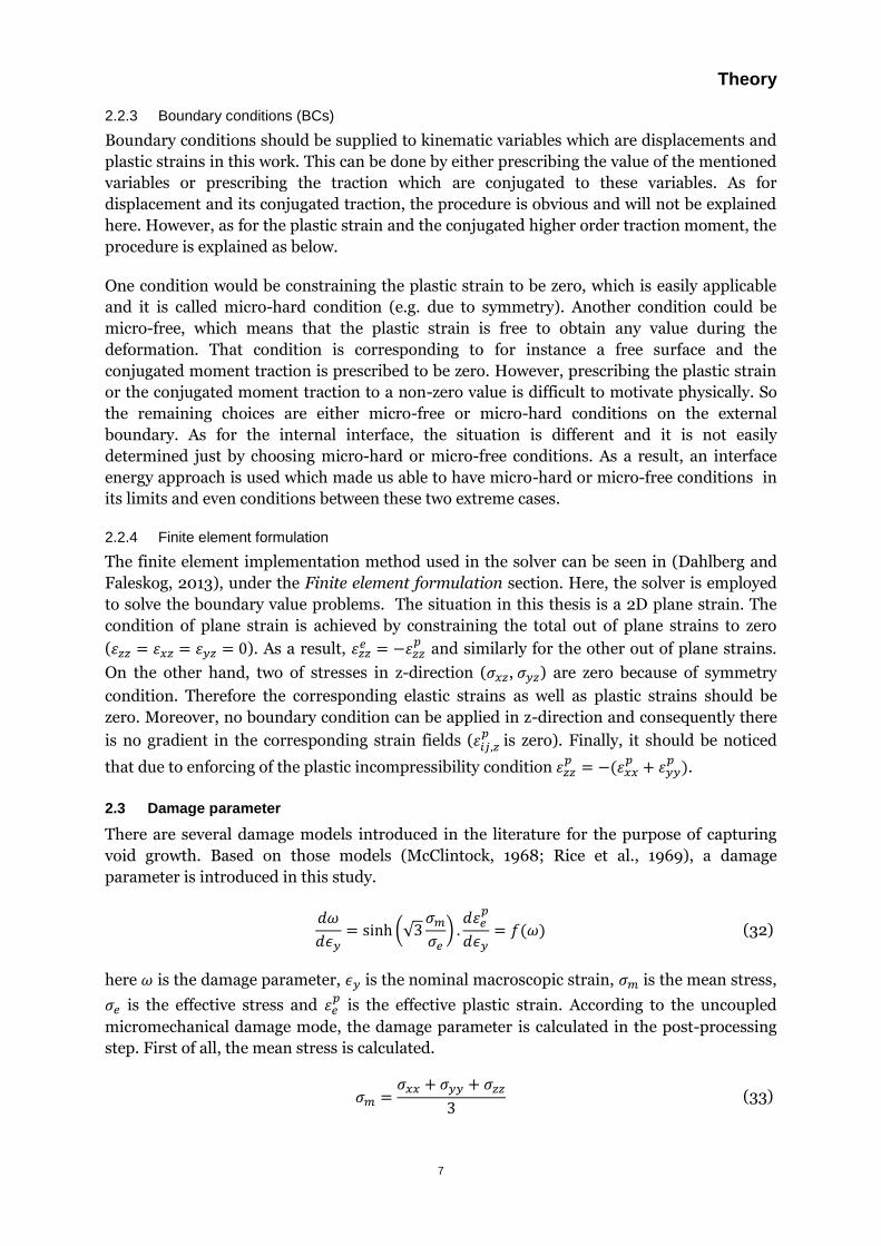
2.3 Damage parameter

There are several damage models introduced in the literature for the purpose of capturing

void growth. Based on those models (McClintock, 1968; Rice et al., 1969), a damage

parameter is introduced in this study.

𝑑𝜔

𝑑𝜖𝑦= sinh (√3

𝜎𝑚𝜎𝑒) .𝑑휀𝑒

𝑝

𝑑𝜖𝑦= 𝑓(𝜔) (32)

here 𝜔 is the damage parameter, 𝜖𝑦 is the nominal macroscopic strain, 𝜎𝑚 is the mean stress,

𝜎𝑒 is the effective stress and 휀𝑒𝑝

is the effective plastic strain. According to the uncoupled

micromechanical damage mode, the damage parameter is calculated in the post-processing

step. First of all, the mean stress is calculated.

𝜎𝑚 =

𝜎𝑥𝑥 + 𝜎𝑦𝑦 + 𝜎𝑧𝑧

3 (33)

Theory

8

where 𝜎𝑖𝑗 is components of the Cauchy stress. The accumulated damage parameter can be

found by the integration of the expression (32).

𝜔 = ∫ 𝑓(𝜔). 𝑑𝜖𝑦

𝜖𝑦,𝑐

0

(34)

here 𝜖𝑦,𝑐 is the nominal macroscopic strain at the selected solution time step. In the post-

processing step, the effective plastic strain increment (Δ휀𝑒𝑝

), mean stress and effective stress

(von Mises) are determined for each solution time step. Then the accumulated damage

parameter is found using the following relation

𝜔 = ∑sinh(√3 (

𝜎𝑚𝜎𝑒)𝑖

) (Δ휀𝑒𝑝)𝑖

𝑛

𝑖=1

(35)

where 𝑖 = 1 and 𝑖 = 𝑛 represent the first and the last solution time steps, respectively. As it

can be seen from the previous relation, the effective plastic strain increment at each step is

amplified by the corresponding stress state triaxiality. It should be noted that the ratio of

mean stress to effective stress represents the stress state triaxiality.

𝑠𝑡𝑟𝑒𝑠𝑠 𝑡𝑟𝑖𝑥𝑖𝑎𝑙𝑖𝑡𝑦 =𝜎𝑚𝜎𝑒

(36)

Model

9

3 Model

3.1 Material properties

The alloy used in this thesis is high-strength A7075-T651 aluminum alloy. As mentioned

before, the 7xxx series of aluminum alloys are influenced by the presence of precipitate-free

zone (PFZ) with a nanoscale width, which is located between the grain interior (bulk) and the

grain boundary (GB). PFZ is created due to quenching after the solution heat treatment and

subsequent ageing. PFZ is softer (with lower yield stress) than bulk hardened by precipitates.

The description of the alloy can be found in a study done by Fourmeau et al. as well as the

PFZ and the bulk material models, see figure 3 in (Fourmeau et al., 2015). W temper is

considered as PFZ representative in a qualitative manner. As for the grain (bulk), T651

temper is used. Assuming PFZ behavior is the same as W temper, some of PFZ features can

be investigated which leads to understanding of ductility reduction of the alloy in the

presence of precipitate-free zone.

The power law hardening for bulk and PFZ can be formulated as

𝜎𝑓 = 𝜎𝑦 (1 +

휀𝑒𝑝

휀0)

𝑁

(37)

where 𝜎𝑦 is yield stress and 휀0 is yield strain. 𝑁 is hardening exponent. 휀𝑒𝑝

is the effective

plastic strain. The yield stress for bulk (𝜎𝑦,𝑏𝑢𝑙𝑘 = 540 𝑀𝑃𝑎) is about three times bigger than

the yield stress for PFZ (𝜎𝑦,𝑃𝐹𝑍 = 170 𝑀𝑃𝑎). However the hardening exponent is 0.084 for

bulk which is lower than 0.24 for PFZ, so the material work hardens more in PFZ. The

Young’s modulus for both (PFZ and bulk) is 𝐸 = 70 𝐺𝑃𝑎 and the Poisson’s ratio is 𝜈 = 0.3.

Finally, bearing in mind that PFZ, which is generally believed as a pure aluminum zone inside

a harder matrix, includes non-negligible amounts of alloying elements in solid solution, and

consequently its behavior is different from pure aluminum in terms of plastic hardening for

example, see (Fourmeau et al., 2015). That should take into account for the microstructure

modeling.

3.2 Micromechanical model

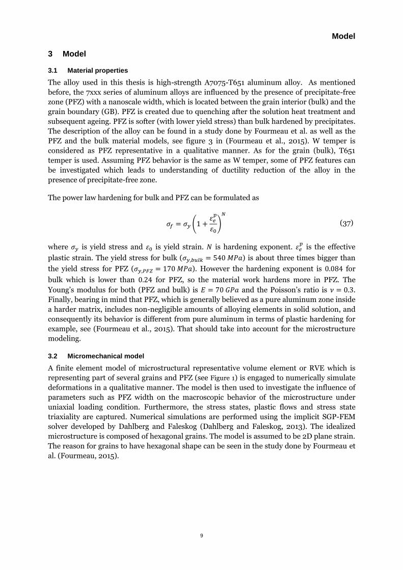
A finite element model of microstructural representative volume element or RVE which is

representing part of several grains and PFZ (see Figure 1) is engaged to numerically simulate

deformations in a qualitative manner. The model is then used to investigate the influence of

parameters such as PFZ width on the macroscopic behavior of the microstructure under

uniaxial loading condition. Furthermore, the stress states, plastic flows and stress state

triaxiality are captured. Numerical simulations are performed using the implicit SGP-FEM

solver developed by Dahlberg and Faleskog (Dahlberg and Faleskog, 2013). The idealized

microstructure is composed of hexagonal grains. The model is assumed to be 2D plane strain.

The reason for grains to have hexagonal shape can be seen in the study done by Fourmeau et

al. (Fourmeau, 2015).

Model

10

a) Microstructure b) RVE

Figure 1: a) Columnar microstructure (plane strain) with hexagonal grains. The representative volume element (RVE) is specified by dashed rectangle. d is the grain size. b) The RVE model.

Bulk region and PFZ (precipitate free zone) are specified by green and orange colors, respectively. The outer blue lines represent the symmetry boundary. The yellow continuous lines show the

grain boundary interfaces and the yellow dashed lines indicate the interfaces between bulk region and PFZ.

As already mentioned PFZ is nanoscale (20 − 40 𝑛𝑚) in size (Fourmeau et al., 2015). On the

other hand the size of grains is found to be about 10 𝜇𝑚. So the ratio of grain size to PFZ

width is between 250 and 500. Numerical simulations using those values are computationally

expensive. As a result, numerical simulations were performed using the ratio of grain size to

PFZ width equal to 20 and then equal to 40 in order to see the influence of the ratio on the

numerical results.

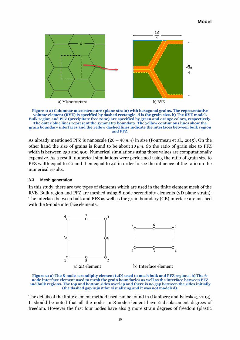
3.3 Mesh generation

In this study, there are two types of elements which are used in the finite element mesh of the

RVE. Bulk region and PFZ are meshed using 8-node serendipity elements (2D plane strain).

The interface between bulk and PFZ as well as the grain boundary (GB) interface are meshed

with the 6-node interface elements.

a) 2D element b) Interface element

Figure 2: a) The 8-node serendipity element (2D) used to mesh bulk and PFZ regions. b) The 6-node interface element used to mesh the grain boundaries as well as the interface between PFZ

and bulk regions. The top and bottom sides overlap and there is no gap between the sides initially (the dashed gap is just for visualizing and it was not modeled).

The details of the finite element method used can be found in (Dahlberg and Faleskog, 2013).

It should be noted that all the nodes in 8-node element have 2 displacement degrees of

freedom. However the first four nodes have also 3 more strain degrees of freedom (plastic

Model

11

strain degrees of freedom). The point of introducing the plastic strains as degrees of freedom

is to constrain the plastic strains of the boundary nodes. As for the 6-node interface element,

the nodes on the bottom side (node number 1, 2 and 3) and the top side (node number 4, 5

and 6) have the same coordinates (overlap) initially. However they can separate or slide

during the deformation of the RVE.

A set of MATLAB scripts is written to generate a mesh for the RVE. The reason for using

several scripts instead of only one script is to make the further implementation easier.

A brief description of some of the main scripts are presented below:

AREAS_DEFINITION: In order to make the mesh generation process easier, the RVE has

been divided into several areas which are meshed separately. The vertices of these areas are

determined and stored in a structure called ‘Area’. Each field of the mentioned structure is a

matrix including the x and y coordinates of vertices (e.g. Area.B1 = [0 0; 0.44 0; 0.22 0.38; 0

0.38]).

Figure 3: Bulk (B) and PFZ (P) areas which are meshed separately. Bulk areas and PFZ areas are shown with green and orange colors, respectively. The grain boundary (GB) interfaces are

specified with continuous lines, whereas the interfaces between the bulk and PFZ areas are shown with dashed lines.

An edge biased structured mesh is used to have more elements in the vicinity of the interfaces

due to the presence of plastic strain gradients. An example of a biased mesh for an arbitrary

area can be seen in Figure 4.

Figure 4: An example of an edge biased structured mesh.

Model

12

𝑙𝑖 = 𝑙1(𝜆)𝑖−1 (38)

𝑙1 = 𝐿

(𝜆 − 1)

𝜆𝑛 − 1 (39)

here 𝐿 is the length of the bottom edge of the area. The parameter 𝜆 is the ratio of 𝑙2 to 𝑙1.

COOR_NOD_AREA: The coordinates of the nodes of each area are determined. First of all,

the four edges of an area are divided to several divisions using the biased mesh method. Then

the coordinates of other points within the area are found. Thirdly, the coordinates of the mid-

points (mid-nodes) are found. Finally, a script called COOR_NOD_AREA_CHECK is created

to make sure that the nodes which are shared between edges have the same coordinates.

ADD_NODE: After finding the coordinates of points and storing them in a matrix variable,

the script is used in order to assign those coordinates to new nodes. The nodes are saved as a

matrix variable which indicates the node number as its first column and the x and 𝑦-

coordinates as its second and third columns, respectively. It should take into consideration

that some areas share the nodes between each other. The shared nodes should have the same

number and coordinates. Consequently, after adding new nodes of each separated area to the

global node variable, a script called DELETE_REDUNDANT_NODE is run to remove

duplicate nodes (e.g. shared nodes on the boundary between F01 and F05 in Figure 3).

ADD_ELEMENT: Now that the nodes of an area are found, the script is utilized to define 8-

node elements (Figure 2). The output of the script is a matrix with n-rows (n is the number of

all elements within the model) and ten columns which stores the element number, material

number and the nodes’ numbers. After meshing all bulk and PFZ areas, a global matrix

variable which has the information about all the elements is generated.

Another point is to store the information about nodes and elements of each area to the

structure variables called ‘PFZ’ and ‘Bulk’ (e.g. ‘Bulk (1).node’ stores the nodes of the area B01

in Figure 3). These structures also should include the information about the nodes on the

boundaries of each area (e.g. ‘Bulk (1).TopEdgeNode’ includes the nodes on the top edge of the

area B01). Those boundary nodes can be used to introduce the interface elements or

boundary conditions.

MESH_INTERFACES: As for the interface elements, the script is developed to get the nodes

on the grain boundaries or between PFZ and bulk areas as the input and generate interface

elements as the output. These interface elements are merged to the global matrix variable.

The first and second trials of mesh generation can be seen in Figure 5. The first trial is not

very successful since it leads to high skewness and the quality of the mesh is not appropriate.

In the second trial it is tried to take advantage of symmetry.

Model

13

a) b)

Figure 5: a) First trial of mesh generation (some elements are skew which lowers the mesh quality and suitability). b) Second trial of mesh generation (taking advantage of symmetry)

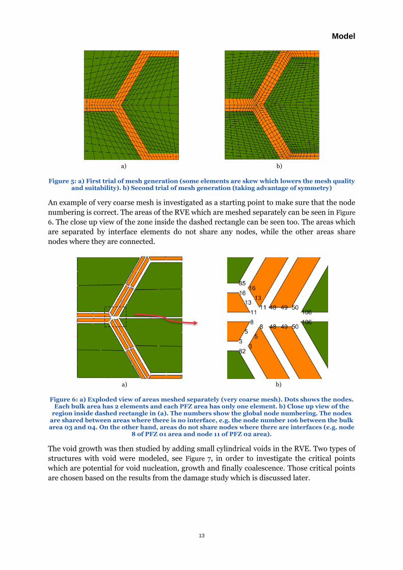
An example of very coarse mesh is investigated as a starting point to make sure that the node

numbering is correct. The areas of the RVE which are meshed separately can be seen in Figure

6. The close up view of the zone inside the dashed rectangle can be seen too. The areas which

are separated by interface elements do not share any nodes, while the other areas share

nodes where they are connected.

a) b)

Figure 6: a) Exploded view of areas meshed separately (very coarse mesh). Dots shows the nodes. Each bulk area has 2 elements and each PFZ area has only one element. b) Close up view of the

region inside dashed rectangle in (a). The numbers show the global node numbering. The nodes are shared between areas where there is no interface, e.g. the node number 106 between the bulk area 03 and 04. On the other hand, areas do not share nodes where there are interfaces (e.g. node

8 of PFZ 01 area and node 11 of PFZ 02 area).

The void growth was then studied by adding small cylindrical voids in the RVE. Two types of

structures with void were modeled, see Figure 7, in order to investigate the critical points

which are potential for void nucleation, growth and finally coalescence. Those critical points

are chosen based on the results from the damage study which is discussed later.

Model

14

a) b)

Figure 7: a) Model with void type-I (very fine mesh). b) Model with void type-II

In order to capture void growth during deformation, spider web grid generation method is

used, Figure 8. The volume of the void is its area multiply the thickness of the model which is

set to unity. Therefore, the expansion of the void is assumed to be proportional only to its

area. The nodes on the voids are stored in a structure variable to be used later. The

circumference of the void is calculated at each time step by knowing the coordinates of those

nodes. Then the circumference is divided by 2𝜋 in order to find the radius of the void at each

step. The important point is that the change in shape of the void is neglected.

Figure 8: Spider web mesh.

The voids are added to the model by manipulating some of the MATLAB scripts. First of all,

each PFZ area was divided to two or three separated zones based on the model with void type.

Then the zone which includes the void is meshed using mapped meshing method, see Figure

9. In the next step, the other zones of each PFZ area are meshed. The mesh generation for

bulk areas do not change significantly.

Figure 9: Mapped meshing which is used to mesh the area around voids (mid-nodes are not shown).

Model

15

After generating mesh using MATLAB scripts, the information about the nodes, elements and

the material properties should be extracted from the model and saved as a text file to be used

as the input required by the solver. The first line of the text file which named ‘Input.txt’ is

about general model dimensions and variables: dimension of the problem (2D), plane type

(plane strain), number of nodes, number of continuum elements, number of interface

elements, number of material sets (2 sets: bulk and PFZ), number of interface material sets (3

sets: grain boundary type I, bulk and PFZ, grain boundary type II), number of material

properties, number of interface properties, number of boundary nodes. Different types of

grain boundary interfaces are shown in Figure 10. The differences between two types is

discussed in section 3.4.

Figure 10: The red lines represent the grain boundary interface type I and the blue lines indicates the grain boundary type II.

After writing the general dimensions of the model in the text file, the material properties are

specified. The material properties are: Young’s modulus (𝐸), Poisson’s ratio (𝜈), yield stress

(𝜎0), hardening exponent (𝑁) and length scale (𝑙). It should be noted that two sets of material

properties are defined, PFZ and bulk materials. Then the interface properties are written in

the text file: 𝐺0. 𝐿+ and 𝐺0. 𝐿

−. As mentioned before, there are three sets of interface

properties. For more information about the parameters see section 2.1. In the next lines of

the text file, the information about nodes and elements are listed. As for nodes, numbers and

coordinates are indicated and as for elements, numbers, material and nodes are written.

Finally the boundary nodes are specified.

3.4 Boundary conditions

Due to symmetry conditions at the boundaries the shear strains are set to zero (𝛾𝑥𝑦 = 0). No

constraints are applied on the normal plastic strains, consequently higher order tractions are

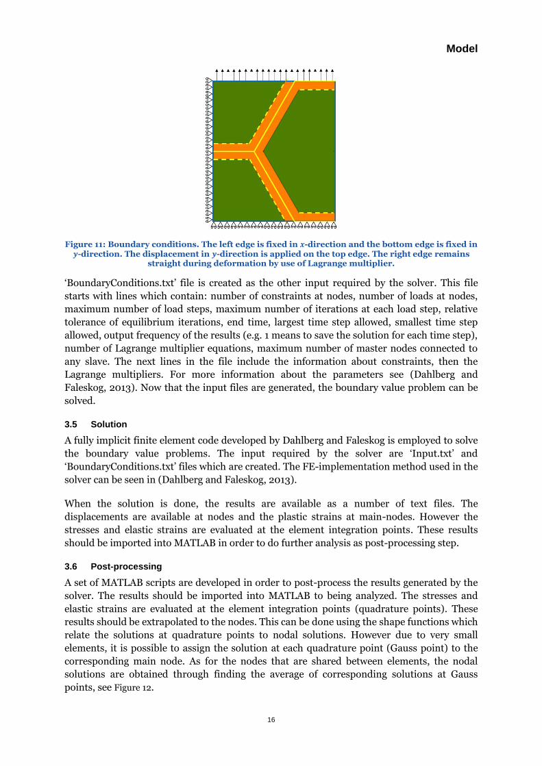
equal to zero (𝑀11 = 𝑀22 = 0). A uniaxial plane strain tension is considered as the loading

condition. The load is chosen as a prescribed displacement on the top edge of the RVE, see

Figure 11. The material experiences yielding, because of the prescribed displacement

magnitude, which is desired. The bottom and left edges are constrained to have zero

displacements. Moreover, Lagrange multiplier is used on the right edge which should stay

straight during deformation.

Model

16

Figure 11: Boundary conditions. The left edge is fixed in 𝒙-direction and the bottom edge is fixed in 𝒚-direction. The displacement in 𝒚-direction is applied on the top edge. The right edge remains

straight during deformation by use of Lagrange multiplier.

‘BoundaryConditions.txt’ file is created as the other input required by the solver. This file

starts with lines which contain: number of constraints at nodes, number of loads at nodes,

maximum number of load steps, maximum number of iterations at each load step, relative

tolerance of equilibrium iterations, end time, largest time step allowed, smallest time step

allowed, output frequency of the results (e.g. 1 means to save the solution for each time step),

number of Lagrange multiplier equations, maximum number of master nodes connected to

any slave. The next lines in the file include the information about constraints, then the

Lagrange multipliers. For more information about the parameters see (Dahlberg and

Faleskog, 2013). Now that the input files are generated, the boundary value problem can be

solved.

3.5 Solution

A fully implicit finite element code developed by Dahlberg and Faleskog is employed to solve

the boundary value problems. The input required by the solver are ‘Input.txt’ and

‘BoundaryConditions.txt’ files which are created. The FE-implementation method used in the

solver can be seen in (Dahlberg and Faleskog, 2013).

When the solution is done, the results are available as a number of text files. The

displacements are available at nodes and the plastic strains at main-nodes. However the

stresses and elastic strains are evaluated at the element integration points. These results

should be imported into MATLAB in order to do further analysis as post-processing step.

3.6 Post-processing

A set of MATLAB scripts are developed in order to post-process the results generated by the

solver. The results should be imported into MATLAB to being analyzed. The stresses and

elastic strains are evaluated at the element integration points (quadrature points). These

results should be extrapolated to the nodes. This can be done using the shape functions which

relate the solutions at quadrature points to nodal solutions. However due to very small

elements, it is possible to assign the solution at each quadrature point (Gauss point) to the

corresponding main node. As for the nodes that are shared between elements, the nodal

solutions are obtained through finding the average of corresponding solutions at Gauss

points, see Figure 12.

Model

17

a) b)

Figure 12: a) Gauss points within an element which are indicated by blue dots. Due to using fine mesh (small elements), the solution in each Gauss point is assigned to the corresponding node. b)

An example of shared node between elements which is specified by red dot. The solutions in corresponding Gauss points are summed and then averaged in order to obtain the nodal solution.

Here a brief description of some of the main scripts for post-processing are presented:

IMPORT_GAUSS_POINTS_DATA: this is the first script in post-processing step which

imports the solutions at Gauss points to the MATLAB workspace. First of all, the stresses and

strains which are saved in ‘CauchyStress.out’, ‘ElasticStrain.out’ and ‘PlasticStrain.out’ files

are imported. Secondly, the area matching to each Gauss point (the element is divided to 4

areas, each corresponding to one Gauss point) is taken from ‘geometry.out’ file. Finally, the

imported values are being used to generate elemental solutions, e.g. the Cauchy stresses at 4

Gauss points within an element are multiplied by their associated areas and then the

summation of resulting values is dived by 4 to find the average. The elemental solutions can

be used to see contour plots. It should take into consideration that those solutions are not

continuous across the elements.

IMPORT_NODES_DOF: The next MATLAB script imports displacements and plastic strains

from ‘dof.out’ text file to MATLAB workspace. This is a tricky task since vertex nodes have 5

degrees of freedom, displacements and plastic strains, while the mid-nodes have only 2

degrees of freedom, only displacements. Therefore an algorithm is written which check the

DOF of each node and then read the values from the text file based on DOF. Finally there is a

command which finds the number of solution time steps and store them as a scalar variable.

It should be stated that all the results imported into workspace are going to be saved as fields

of a structure variable named ‘Sol’, e.g. ‘Sol.Nod(1).EffPlasStrain’ is a vector which contains the

effective plastic strains at each time step.

IMPORT_TRACTIONS: There are also tractions as results which are extracted from ‘tractions.out’ text file using the script. These results contain the force tractions as well as moment tractions (𝑓𝑥 , 𝑓𝑦,𝑀𝑥 ,𝑀𝑦 and 𝑀𝑥𝑦). The force tractions are used to find the nominal

macro stresses.

ANALYSIS: after importing the evaluated results by the solver into MATLAB workspace as

the structure variable (Sol), these results should be analyzed to generate plots. First thing to

do is to calculate the effective plastic strains.

Δ휀𝑒𝑝= √

2

3((Δ휀𝑥𝑥

𝑝)2+ (Δ휀𝑦𝑦

𝑝)2+ (Δ휀𝑥𝑥

𝑝+ Δ휀𝑦𝑦

𝑝)2+ (2Δ휀𝑥𝑦

𝑝)2) (40)

Model

18

then the accumulated value can be obtained

휀𝑒𝑝=∑Δ휀𝑝 (41)

however the effective plastic strains and the other values calculated by the script are only

obtained for main nodes. In fact in plotting contours, only the values at main nodes are going

to be used. These effective values are saved as ‘Sol.Nod.EffPlasStrain’ variable for further

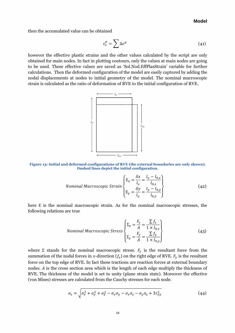
calculations. Then the deformed configuration of the model are easily captured by adding the

nodal displacements at nodes to initial geometry of the model. The nominal macroscopic

strain is calculated as the ratio of deformation of RVE to the initial configuration of RVE.

Figure 13: Initial and deformed configurations of RVE (the external boundaries are only shown). Dashed lines depict the initial configuration.

𝑁𝑜𝑚𝑖𝑛𝑎𝑙 𝑀𝑎𝑐𝑟𝑜𝑠𝑐𝑜𝑝𝑖𝑐 𝑆𝑡𝑟𝑎𝑖𝑛

{

Εx =

𝛿𝑥

𝑙𝑥=𝑙𝑥 − 𝑙0,𝑥𝑙0,𝑥

Εy =𝛿𝑦

𝑙𝑦=𝑙𝑦 − 𝑙0,𝑦

𝑙0,𝑦 }

(42)

here Ε is the nominal macroscopic strain. As for the nominal macroscopic stresses, the

following relations are true

𝑁𝑜𝑚𝑖𝑛𝑎𝑙 𝑀𝑎𝑐𝑟𝑜𝑠𝑐𝑜𝑝𝑖𝑐 𝑆𝑡𝑟𝑒𝑠𝑠

{

Σx =

𝐹𝑥𝐴=

∑𝑓𝑥1 × 𝑙0,𝑥

Σy =𝐹𝑦

𝐴=

∑𝑓𝑦

1 × 𝑙0,𝑦}

(43)

where Σ stands for the nominal macroscopic stress. 𝐹𝑥 is the resultant force from the

summation of the nodal forces in 𝑥-direction (𝑓𝑥) on the right edge of RVE. 𝐹𝑦 is the resultant

force on the top edge of RVE. In fact these tractions are reaction forces at external boundary

nodes. 𝐴 is the cross section area which is the length of each edge multiply the thickness of

RVE. The thickness of the model is set to unity (plane strain state). Moreover the effective

(von Mises) stresses are calculated from the Cauchy stresses for each node.

𝜎𝑒 = √𝜎𝑥

2 + 𝜎𝑦2 + 𝜎𝑧

2 − 𝜎𝑥𝜎𝑦 − 𝜎𝑥𝜎𝑧 − 𝜎𝑦𝜎𝑧 + 3𝜏𝑥𝑦2 (44)

Model

19

Other quantities of interest are the mean stress and stress triaxiality which are used to find

the damage parameter. The mean stress is calculated as below

𝜎𝑚 =

𝜎𝑥 + 𝜎𝑦 + 𝜎𝑧

3 (45)

where 𝜎 is the Cauchy stress. Then the stress triaxiality is found using the following relation

𝑠𝑡𝑟𝑒𝑠𝑠 𝑡𝑟𝑖𝑎𝑥𝑖𝑎𝑙𝑖𝑡𝑦 =𝜎𝑚𝜎𝑒

(46)

where 𝜎𝑒 is the effective stress. Knowing the stress triaxiality and the effective plastic strain,

one can find the damage parameter. The damage parameter is found for each step and

considered as an incremental variable.

Δ𝐷 = sinh(𝑠𝑞𝑟𝑡(𝑠𝑡𝑟𝑒𝑠𝑠 𝑡𝑟𝑖𝑎𝑥𝑖𝑎𝑙𝑖𝑡𝑦)) Δεe𝑝

(47)

the incremental damage is saved as ‘Sol.Nod.Damage.Del’.Then the accumulated damage is calculated as the sum of the increments and it is stored as a variable named ‘Sol.Nod.Damage.Sum’. Moreover the maximum value of effective plastic strain is found at each time step which is used as a criteria for mesh convergence study.

CONTOUR_PLOT: the contours are plotted for different purposes such as the effective

plastic strain. The plots are generated using the ‘pcolor’ command in MATLAB. There is an

option of ‘pcolor’ command which is ‘shading interp’ which varies the color in each line

segment and face by interpolating the colormap index or true color value across the line or

face2. However using this option leads to taking so much time to generate plots. Therefore the

option is not used and instead the average value of nodal solutions for each element is

determined and used to generate contour plots.

2 MATLAB online help

Results and discussion

20

4 Results and discussion

4.1 Parametric study

In order to understand the effects of material and interface parameters on the overall

behavior of the microstructure, a number of parametric studies are performed by changing

some parameters while keeping others constant. The nominal macroscopic stress-strain

curves are acquired as a representative of the microstructure overall behavior. The

unchanged bulk material properties are: 𝐸 𝜎0,𝑏𝑢𝑙𝑘⁄ = 130, 𝜈 = 0.3, 𝑛 = 500, 휀0̇ = 0.04, 𝜇 =

2, 𝜅 = 0.00001, 휀0,𝑏𝑢𝑙𝑘 = 𝜎0,𝑏𝑢𝑙𝑘 𝐸⁄ and 𝑛𝑏𝑢𝑙𝑘 = 0.084 (see section 2.2.1 and 3.1 for definition

of parameters). As for PFZ material properties, most of the properties are the same as bulk

except for: 𝜎0,𝑃𝐹𝑍 𝜎0,𝑏𝑢𝑙𝑘⁄ = 0.32, 휀0,𝑃𝐹𝑍 = 0025 and 𝑛𝑃𝐹𝑍 = 0.24. The constitutive equations

for the interface are described in detail in section 2.2.2. The stiffness for the elastic

deformation at the interface is set to 𝐶. 𝑑 𝜎0,𝑏𝑢𝑙𝑘⁄ = 3.107, where 𝑑 is the grain size. The

interface hardening is 𝐻𝑠. 𝑑 𝜎0,𝑏𝑢𝑙𝑘⁄ = 10. The constant parameters for the energetic interface

are: 𝐺0 𝜎0,𝑏𝑢𝑙𝑘⁄ = 50, 휀0 = 0.4 𝜎0,𝑏𝑢𝑙𝑘 𝐸⁄ and 𝐿− of the grain boundary interface is set to a very

large value. The latter parameter is chosen in a way that there is no plastic strains mismatch

across the grain boundary interface due to having the same material (PFZ) on both sides of

this interface. The parameters for the energy potential (Ψ) are: 𝑝 = 6, 𝑞 = 2 and 𝜂 = 1 see

(Dahlberg and Faleskog, 2013).

The following expressions are developed to make the changing parameters easier to

manipulate

𝑀+ = 𝐺0휀0𝐿+ (48)

𝑀+ = 10 𝜎0,𝑏𝑢𝑙𝑘 𝑙𝑏𝑢𝑙𝑘 (49)

𝐺0 = 0.4 𝐸 (50)

휀0,𝑖𝑛𝑡𝑒𝑟𝑓𝑎𝑐𝑒 = 𝜂𝜎0,𝑏𝑢𝑙𝑘𝐸

(51)

therefore

0.4 𝐸 𝐿+ 𝜂 𝜎0,𝑏𝑢𝑙𝑘𝐸

= 10 𝜎0,𝑏𝑢𝑙𝑘 𝑙𝑏𝑢𝑙𝑘 (52)

as a result

𝐿+ = 𝑙𝑏𝑢𝑙𝑘

10

0.4 𝜂 (53)

finally

𝐿+ = 𝑙𝑏𝑢𝑙𝑘

25

𝜂 (54)

using the expression (54), one can change 𝜂 in order to change 𝐿+ for the interfaces.

The following parameters are used in all the studies unless something else is stated.


21

𝑑 = 1, 2ℎ 𝑑⁄ = 0.05,

𝜂𝐵𝑃 = 64, 𝜂𝐺𝐵 = 64,

𝐿𝐵𝑃− 𝑑⁄ = 10−5 , 𝐿𝐺𝐵

− 𝑑⁄ = 4000,

𝑙𝑏𝑢𝑙𝑘 𝑑⁄ = 0.1, 𝑙𝑃𝐹𝑍 𝑑⁄ = 0.1

(55)

where 𝑑 is the grain size, 2ℎ is the PFZ width, 𝐵𝑃 stands for the interface between bulk and

PFZ, 𝐺𝐵 means grain boundary interface and 𝑙 is the material length scale.

Figure 14: Amount of effective plastic strain (𝜺𝒆𝒑), stress state triaxiality (𝝈𝒎 𝝈𝒆⁄ ), damage

parameter (𝝎) and effective stress (𝝈𝒆) along the yellow line (𝑺) indicated in the first shape.


22

The amounts of effective plastic strain, stress state triaxiality, damage and effective stress are

determined along the yellow line in Figure 14. The line is located in the middle of PFZ. The

damage parameter is a function of plastic strain which is amplified by the stress state

triaxiality. Therefore the maximum damage value is located at the point where the values of

stress state triaxiality and effective plastic strain are maximum.

4.1.1 Mesh convergence

A mesh convergence study is performed. The nominal macroscopic stress-strain curves are

generated using different number of elements (different element sizes). The number of

divisions along PFZ is defined as a parameter called ‘𝑁𝑜. 𝑒𝑙. 𝑥’ and the number of divisions

across PFZ thickness is called ‘𝑁𝑜. 𝑒𝑙. 𝑡’, see Figure 15. The generated macroscopic stress-

strain curves can be seen in Figure 16 and Figure 17Figure 15. It should be noted that the red

and blue solid lines show the material models for PFZ and bulk, respectively. The

micromechanical model consists of both PFZ and bulk region, therefore the resultant

material model is different from PFZ and bulk models. Moreover, the micromechanical

model generally has higher macroscopic yield stress due to presence of the interfaces which

acts as barriers against dislocation motions.

Figure 15: The number of elements along PFZ is named as No.el.t and the number of elements

across its thickness is called No.el.x.


23

Figure 16: Nominal macroscopic stress-strain curves (uniaxial loading) for different number of

elements along PFZ (No.el.x). The red and blue solid line show PFZ and bulk material models.

Figure 17: Nominal macroscopic stress-strain curves for different number of elements across PFZ

width (No.el.t).


24

As it is clear from Figure 16, all the studies lead to mostly the same macroscopic behavior and

from Figure 17, one can see that the number of elements across PFZ width change the

macroscopic behavior of the model. However it would be useful to compare the resultant

maximum effective plastic strain within the model using various number of elements, Figure

18.

Figure 18: The influence of number of parameters on the maximum effective plastic strain within the model

It can be seen from the previous figure that the number of elements have impact on the

maximum plastic strain. The maximum value of plastic strain is converged using 30 elements

along PFZ. However using 30 elements is computationally expensive. Therefore 20 is chosen

as the value of 𝑁𝑜. 𝑒𝑙. 𝑥. From Figure 17 for the number of elements across PFZ, 6 is chosen as

an appropriate value. So these number of elements are used in all the studies unless

something else is stated.

4.1.2 Interface length scales (𝐿−, 𝐿+)

The value of 𝐿− for the interface between PFZ and bulk is investigated. Since the material

property on one side of this interface is different from the material property on the other side,

no penalty should exist on the plastic strain mismatch across that interface. However it is

observed that the solution does not converge by setting a value of 𝐿− that is too small.

Therefore a study of 𝐿− magnitude is performed and it is seen that the magnitudes less than

10−5𝑑 lead to the same macroscopic behavior, see Figure 19. Therefore the 10−5𝑑 is chosen

as the optimal value.

In the next step, the amount of 𝐿𝐺𝐵− (GB: grain boundary) is studied. The material properties

are the same for both sides of the grain boundary interface, therefore high penalty should be

imposed in order to make sure that there is almost no strain mismatch across the interface. It


25

can be seen from Figure 20, that all the values of 𝐿𝐺𝐵− lead to the same result. Consequently

𝐿𝐺𝐵− = 4000𝑑 is chosen.

Figure 19: The study of 𝐋− of the interface between bulk and PFZ.

Figure 20: The study of 𝑳𝑮𝑩

− , GB stands for grain boundary.


26

The length scales (𝐿+) of the grain boundary interface and the interface between bulk and

PFZ are studied and the results are discussed in this section. In fact 𝐿+ penalizes the amount

of plastic strains, consequently increasing the value of interface length scale leads to higher

gradients in plastic strains on both sides of the interface. It should be noted that 𝐿+ is defined

as a function of 𝜂, expression (54), therefore the figures for 𝐿+ investigation is based on 𝜂 and

a higher value of 𝜂 corresponds to a lower value of 𝐿+.

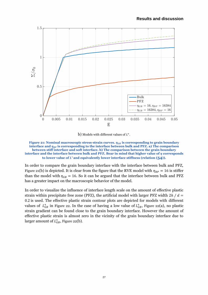
The value of 𝐿+ has an impact on the macroscopic behavior of the model, see Figure 21(a). The

slope of the stress-strain curves after yield onset is raised by increasing the value of 𝐿+ (or

equivalently decreasing 𝜂 parameter). In addition the yield stress is increased. Since the

stress corresponding to a specific strain (e.g. 0.05) is higher for the model with greater 𝐿+

magnitudes, an argument can be formulated as ‘increasing 𝐿+ makes the RVE model stiffer’.

The relation between the interface stiffness, which is proportional to 𝐿+, and the stresses in

PFZ and bulk regions is summarized as below.

The external work is equal to the internal work. The internal energy is the sum of elastic

strain energy, dissipated energy due to plastic deformation as well as the stored energy in

interfaces. Moreover, the amount of energy stored in interfaces depends on the 𝐿+ value. So if

the value of 𝐿+ changes, the amount of stored energy in interfaces will change. Consequently

the total amount of strain and dissipated energy in bulk and PFZ will change. As a result the

stresses in bulk and PFZ will change too.

a) Models with equal values of 𝐿+ of the interfaces (𝐿𝐺𝐵

+ = 𝐿𝐵𝑃+ or equivalently 𝜂𝐺𝐵 = 𝜂𝐵𝑃).


27

b) Models with different values of 𝐿+.

Figure 21: Nominal macroscopic stress-strain curves. 𝜼𝑮𝑩 is corresponding to grain boundary interface and 𝜼𝑩𝑷 is corresponding to the interface between bulk and PFZ. a) The comparison

between stiff interface and soft interface. b) The comparison between the grain boundary interface and the interface between bulk and PFZ. Bear in mind that higher value of 𝜼 corresponds

to lower value of 𝑳+and equivalently lower interface stiffness (relation (54)).

In order to compare the grain boundary interface with the interface between bulk and PFZ,

Figure 21(b) is depicted. It is clear from the figure that the RVE model with 𝜂𝐵𝑃 = 16 is stiffer

than the model with 𝜂𝐺𝐵 = 16. So it can be argued that the interface between bulk and PFZ

has a greater impact on the macroscopic behavior of the model.

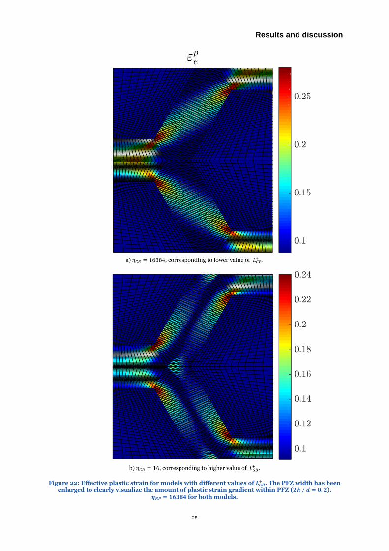
In order to visualize the influence of interface length scale on the amount of effective plastic

strain within precipitate free zone (PFZ), the artificial model with larger PFZ width 2ℎ ⁄ 𝑑 =

0.2 is used. The effective plastic strain contour plots are depicted for models with different

values of 𝐿𝐺𝐵+ in Figure 22. In the case of having a low value of 𝐿𝐺𝐵

+ , Figure 22(a), no plastic

strain gradient can be found close to the grain boundary interface. However the amount of

effective plastic strain is almost zero in the vicinity of the grain boundary interface due to

larger amount of 𝐿𝐺𝐵+ , Figure 22(b).


28

a) 𝜂𝐺𝐵 = 16384, corresponding to lower value of 𝐿𝐺𝐵

+ .

b) 𝜂𝐺𝐵 = 16, corresponding to higher value of 𝐿𝐺𝐵

+ .

Figure 22: Effective plastic strain for models with different values of 𝑳𝑮𝑩+ . The PFZ width has been

enlarged to clearly visualize the amount of plastic strain gradient within PFZ (𝟐𝒉 ⁄ 𝒅 = 𝟎. 𝟐). 𝜼𝑩𝑷 = 𝟏𝟔𝟑𝟖𝟒 for both models.


29

4.1.3 Material length scale (𝑙)

The length scales of bulk and PFZ are established as changing parameters in this step.

Altering the length scales changes the length which is needed for the plastic strain to increase

from a minimum value to a maximum value. In other words, the length over which the plastic

strain gradient is present is proportional to the length scale. The length scale of bulk is

normalized with grain size and the length scale of PFZ is normalized with respect to PFZ

thickness (ℎ, which is half PFZ width).

a) Models with equal bulk and PFZ material length scales (𝑙𝑏𝑢𝑙𝑘 = 𝑙𝑃𝐹𝑍).


30

b) Models with different bulk and PFZ material length scales.

Figure 23: Nominal macroscopic stress-strain curves for models with various material length

scales. The value of 𝑳+ has been kept constant for all models.

As it is clear from Figure 23, the amount of material length scale has a significant effect on

the macroscopic behavior. After yielding point, the slope of the stress-strain curves depends

significantly on the length scale and increasing the length scale makes the model work

hardens more. Equivalently it can be argued that for the same amount of total strain, the

corresponding stress value rises by increasing the length scale. This is due to the fact that the

plastic strain gradient is present over a larger distance by increasing the length scale and

consequently the total amount of plastic strain decreases.

In order to visualize the influence of material length scale on the amount of effective plastic

strain within precipitate free zone (PFZ), the artificial model with larger PFZ’s width 2ℎ ⁄ 𝑑 =

0.2 has been used. The value of PFZ material length scale (𝑙𝑃𝐹𝑍) normalized by the grain size

(𝑑) is raised from 0.01 to 0.1, Figure 24.

As it is clear from Figure 24, the effective plastic strain is decreased by the factor two and the

plastic strain gradient appears over larger area. This is due to the fact that increasing 𝑙/𝑑

introduces higher constrains on the amount of plastic strain gradient.


31

a) 𝑙𝑃𝐹𝑍/𝑑 = 0.01

b) 𝑙𝑃𝐹𝑍/𝑑 = 0.1

Figure 24: Effective plastic strain for models with different PFZ material length scales (𝒍𝑷𝑭𝒁). The PFZ width has been enlarged to clearly visualize the amount of plastic strain gradients within PFZ

(𝟐𝒉 ⁄ 𝒅 = 𝟎. 𝟐).


32

4.2 Models with and without PFZ

In this section, the models with and without PFZ are compared to understand the role of PFZ

on the ductility reduction. It should be noted that the amount of 𝐿𝐵𝑃+ is set to a lower value

compared to the value of 𝐿𝐺𝐵+ , since the interface between bulk and PFZ is not a true physical

interface. In fact the dislocation is free to move from bulk region to PFZ, except that the

density of dislocations is higher in the softer zone (PFZ), therefore the dislocations pile up at

the boundary between bulk and PFZ.

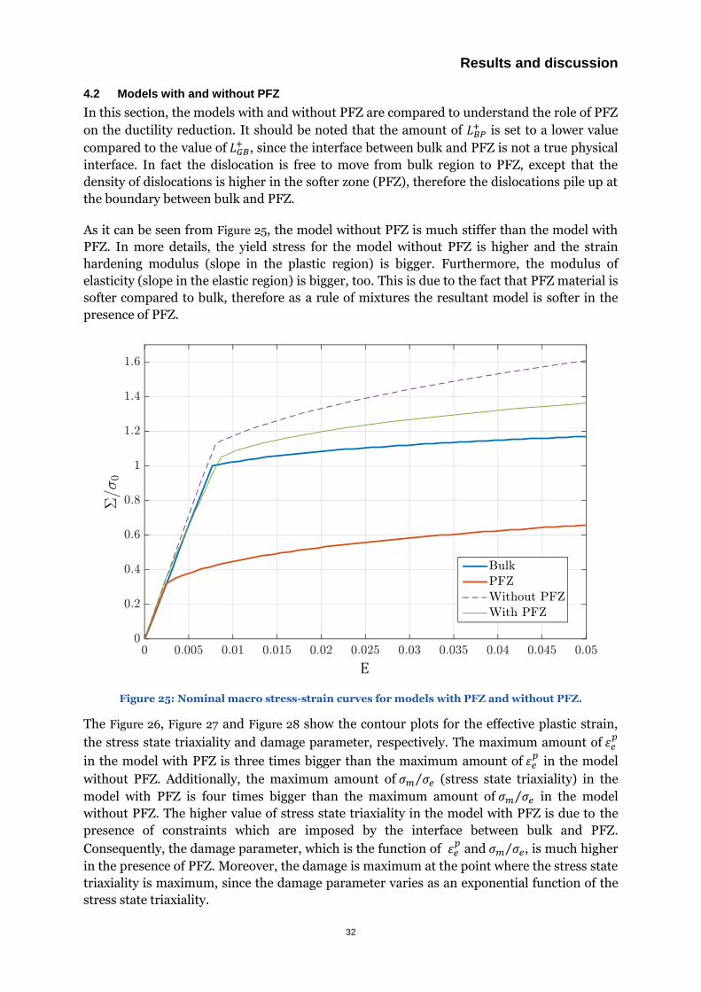
As it can be seen from Figure 25, the model without PFZ is much stiffer than the model with

PFZ. In more details, the yield stress for the model without PFZ is higher and the strain

hardening modulus (slope in the plastic region) is bigger. Furthermore, the modulus of

elasticity (slope in the elastic region) is bigger, too. This is due to the fact that PFZ material is

softer compared to bulk, therefore as a rule of mixtures the resultant model is softer in the

presence of PFZ.

Figure 25: Nominal macro stress-strain curves for models with PFZ and without PFZ.

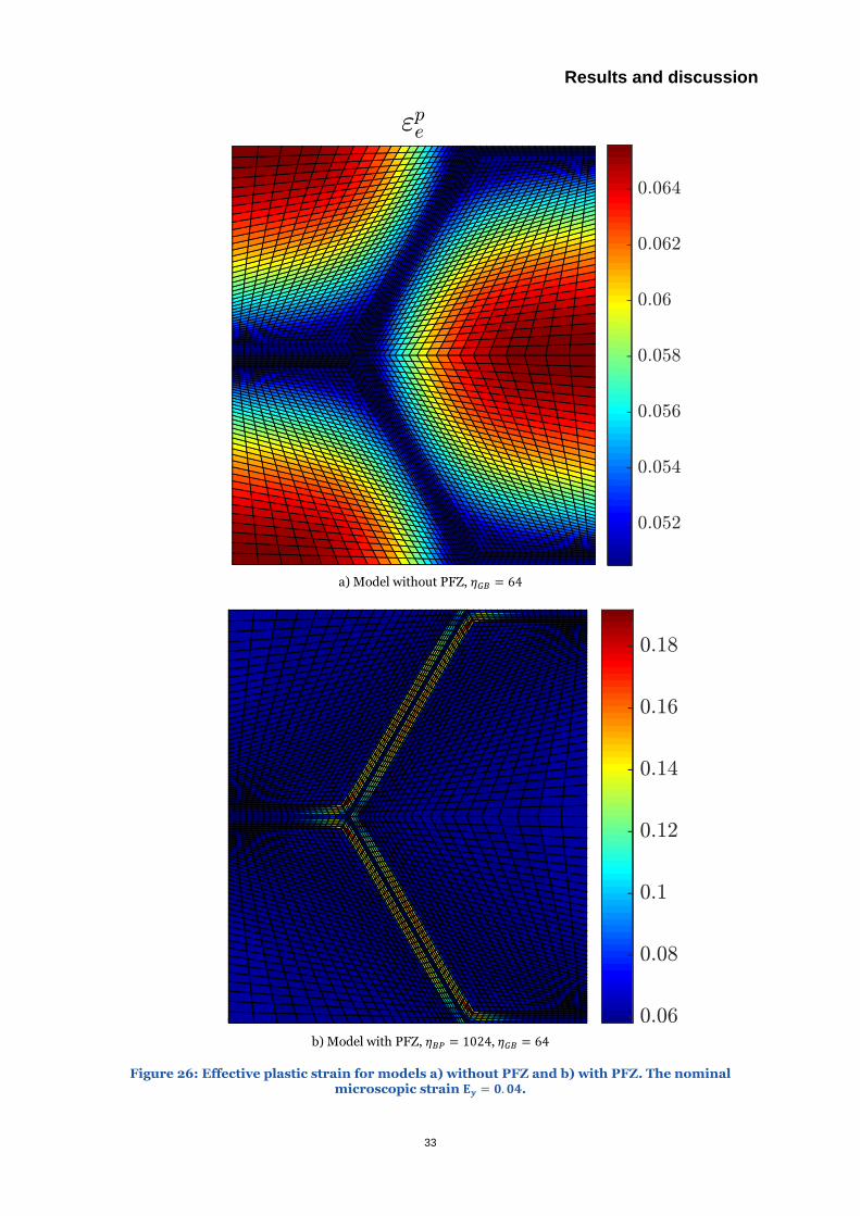
The Figure 26, Figure 27 and Figure 28 show the contour plots for the effective plastic strain,

the stress state triaxiality and damage parameter, respectively. The maximum amount of 휀𝑒𝑝

in the model with PFZ is three times bigger than the maximum amount of 휀𝑒𝑝

in the model

without PFZ. Additionally, the maximum amount of 𝜎𝑚 𝜎𝑒⁄ (stress state triaxiality) in the

model with PFZ is four times bigger than the maximum amount of 𝜎𝑚 𝜎𝑒⁄ in the model

without PFZ. The higher value of stress state triaxiality in the model with PFZ is due to the

presence of constraints which are imposed by the interface between bulk and PFZ.

Consequently, the damage parameter, which is the function of 휀𝑒𝑝

and 𝜎𝑚 𝜎𝑒⁄ , is much higher

in the presence of PFZ. Moreover, the damage is maximum at the point where the stress state

triaxiality is maximum, since the damage parameter varies as an exponential function of the

stress state triaxiality.


33

a) Model without PFZ, 𝜂𝐺𝐵 = 64

b) Model with PFZ, 𝜂𝐵𝑃 = 1024, 𝜂𝐺𝐵 = 64

Figure 26: Effective plastic strain for models a) without PFZ and b) with PFZ. The nominal microscopic strain 𝚬𝒚 = 𝟎. 𝟎𝟒.


34



Figure 27: Stress state triaxiality for models a) without PFZ and b) with PFZ. The nominal microscopic strain 𝚬𝒚 = 𝟎. 𝟎𝟒.


35



Figure 28: Accumulated damage for models a) without PFZ and b) with PFZ. The nominal macroscopic strain 𝚬𝒚 = 𝟎. 𝟎𝟒.


36

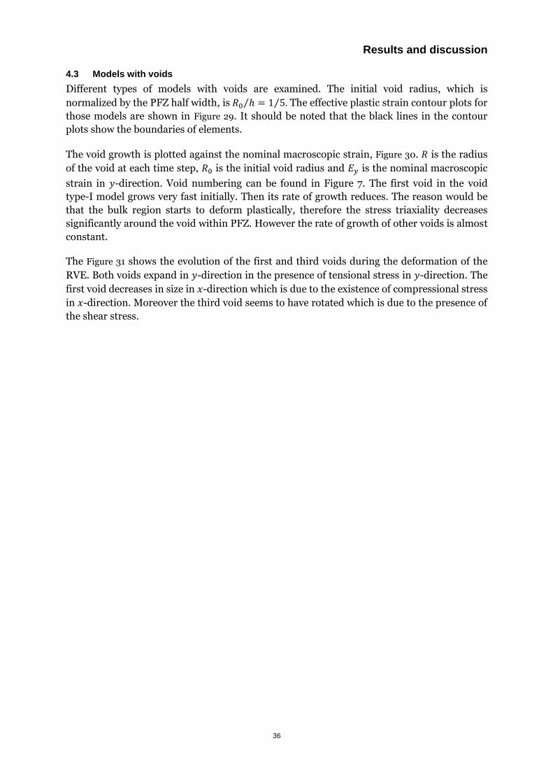
4.3 Models with voids

Different types of models with voids are examined. The initial void radius, which is

normalized by the PFZ half width, is 𝑅0 ℎ⁄ = 1 5⁄ . The effective plastic strain contour plots for

those models are shown in Figure 29. It should be noted that the black lines in the contour

plots show the boundaries of elements.

The void growth is plotted against the nominal macroscopic strain, Figure 30. 𝑅 is the radius

of the void at each time step, 𝑅0 is the initial void radius and 𝐸𝑦 is the nominal macroscopic

strain in 𝑦-direction. Void numbering can be found in Figure 7. The first void in the void

type-I model grows very fast initially. Then its rate of growth reduces. The reason would be

that the bulk region starts to deform plastically, therefore the stress triaxiality decreases

significantly around the void within PFZ. However the rate of growth of other voids is almost

constant.

The Figure 31 shows the evolution of the first and third voids during the deformation of the

RVE. Both voids expand in 𝑦-direction in the presence of tensional stress in 𝑦-direction. The

first void decreases in size in 𝑥-direction which is due to the existence of compressional stress

in 𝑥-direction. Moreover the third void seems to have rotated which is due to the presence of

the shear stress.


37

a) Void type-I.

b) Void type-II.

Figure 29: Effective plastic strain for models with voids.


38

Figure 30: Void growth vs. nominal macroscopic strain, 𝑹 is the radius of the void at each step, 𝑹𝟎 is the initial void radius and 𝑬𝒚 is the nominal macroscopic strain in 𝒚-direction. 𝑹𝟎 𝒉⁄ = 𝟏 𝟓⁄ . Void

numbering is based on Figure 7.

a) Void 1, type-I


39

b) Void 3, type-I

Figure 31: Examples of void evolutions. The dashed blue circles show the void with initial

configuration (1st step) which is moved.

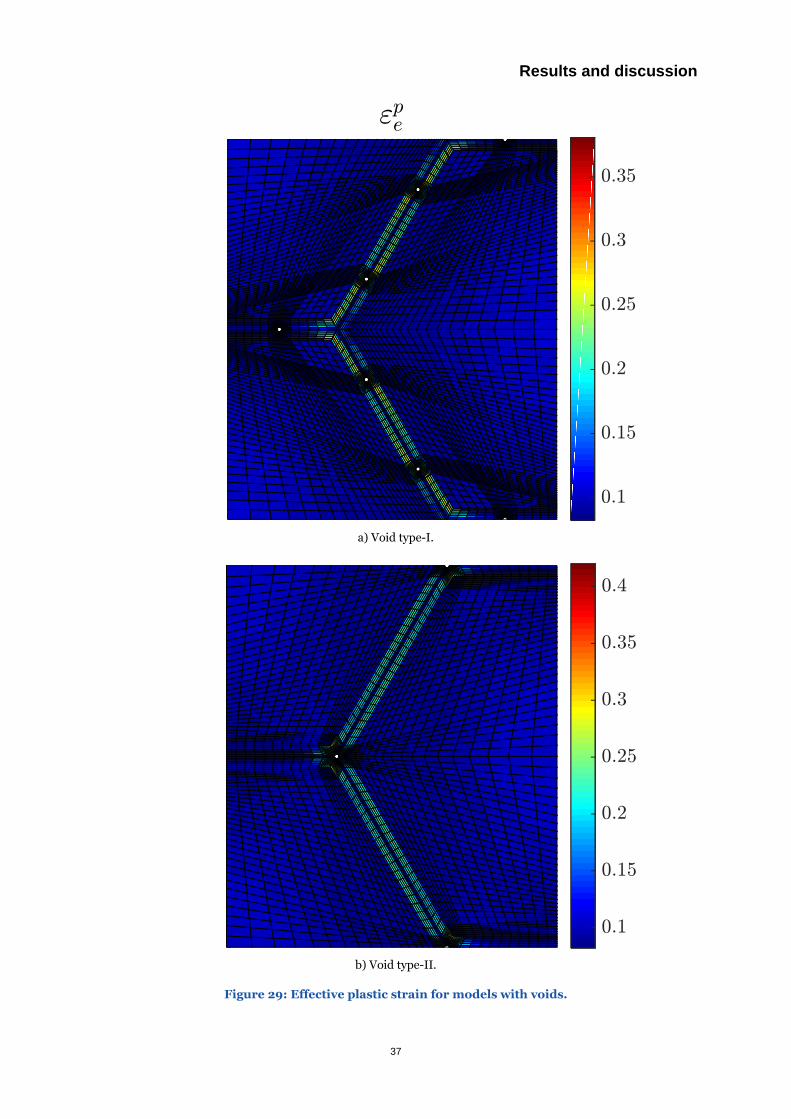
4.4 PFZ width investigation

In this section, PFZ width is studied. As it can be seen from the Figure 32, the yield stress

increases as PFZ width decreases since the volume fraction of softer material (PFZ) is

reduced. Additionally, the maximum amounts of effective plastic strain and damage

parameter within the RVE are plotted against PFZ width normalized by the grain size (2ℎ 𝑑⁄ ),

see Figure 33. The amount of maximum damage parameter increases by reducing PFZ width.

Therefore it can be argued that for the model of RVE with real PFZ thickness which is

computationally expensive to be solved, the maximum amount of damage would be very

high. Equivalently, the possibility of void growth inside PFZ would be very high.

Finally the effective plastic strain is plotted against nominal macroscopic strain, see Figure 34.

The solid lines and dashed lines are corresponding to effective plastic strain evolution in PFZ

and effective plastic strain in bulk region, respectively. It is obvious that the plastic

deformation is much higher in PFZ compared to bulk region. Moreover, plastic deformation

of the model with thicker PFZ is lower than the model with thinner PFZ.


40

Figure 32: Nominal macro stress-strain curves for models with different PFZ widths (𝟐𝒉).

a)


41

b)

Figure 33: Maximum values of a) effective plastic strain and b) accumulated damage vs. PFZ widths (𝟐𝒉). The nominal macroscopic strain 𝚬𝒚 = 𝟎.𝟎𝟒.

Df

Figure 34: Evolution of effective plastic strain of nodes with maximum values in PFZ and bulk region.

Conclusion

42

5 Conclusion

The influence of precipitate-free zone (PFZ) on the ductility reduction is investigated for the

hexagonal grain structure of the high-strength A7075-T651 aluminum alloy. PFZ is softer

material, having lower yield stress, compared to bulk (grain interior) material and it is

located along the grain boundaries (GB). The analysis is carried out using strain gradient

plasticity (SGP). The grain boundaries and the boundary between PFZ and bulk region are

modeled with interface elements. In fact, an interface is considered as a barrier to dislocation

motion, therefore using the interfaces leads to non-uniform plastic strain within the model.

As a result plastic strain gradients are introduced. These gradients are influential if they

occur over a distance comparable to the material length scale (𝑙). The length scale is a

phenomenological material parameter representing the scale at which the plastic strain

gradients are present. A damage parameter is defined which is representative of void growth

rate.

The representative volume element (RVE) of the microstructure is modeled. The uniaxial

loading condition is achieved by prescribed displacement on the top boundary edge of the

RVE. The nominal macroscopic strain and stress are defined and the stress-strain curves are

considered as the representative of the macroscopic behavior of the model. Several

parametric studies are performed in order to understand the role of each parameter on the

macroscopic behavior. Moreover, the models with and without PFZ are compared to

understand the role of PFZ in ductility reduction. Additionally, the real voids are modeled

within PFZ and the evolution of them during deformation are monitored. Finally, PFZ width

is examined to see the change in the maximum damage parameter which is proportional to

void growth rate.

One of the main results of the present study is the comparison of the amount of damage

parameter between the model with PFZ and the model without PFZ, Figure 28. As it can be

seen from the figure, the maximum amount of accumulated damage is much higher in the

model with PFZ. Consequently, it can be argued that the possibility of void nucleation,

growth and coalescence is much higher in the presence of PFZ.

Another point is that the amount of maximum plastic strain increases by making the PFZ

thinner, in spite of the fact that the volume fraction of PFZ, which has lower yield stress,

decreases and consequently the maximum damage parameter also rises, Figure 33.

It should be noted that the choice of an isotropic models for PFZ and bulk as well as the use

of hexagonal grain structure are simplifications. In fact the present thesis is a qualitative

study with focus on understanding the PFZ and bulk material properties as well as the

interfaces features. Therefore, the results are supposed to give understanding of the role of

PFZ on the ductility reduction.

As for the further studies, it would beneficial to add finite strain to the solver then look at the

void growth and find the critical points with high possibility of failure. Moreover, it is

desirable to also add voids to bulk region and then look at the void growth for models with

PFZ and without PFZ.

References

43

6 References

Dahlberg CF, Gudmundson P (2008). Hardening and softening mechanisms at decreasing microstructural length scales. Philosophical Magazine 88.30-32, 3513-3525.

Dahlberg CF, Faleskog J (2013) An improved strain gradient plasticity formulation with energetic interfaces: theory and a fully implicit finite element formulation. Comput. Mech. 51, 641–659.

Dahlberg CF, Faleskog J, Niordson CF, Legarth BN (2013). A deformation mechanism map for polycrystals modeled using strain gradient plasticity and interfaces that slide and separate. International Journal of Plasticity 43, 177-195.

Evans AG, Hutchinson JW (2009). A critical assessment of theories of strain gradient plasticity. Acta Materialia 57.5, 1675-1688.

Fleck NA, Hutchinson JW (1997). Strain gradient plasticity. Advances in applied mechanics 33, 296-361.

Fleck NA, Willis JR (2009). A mathematical basis for strain-gradient plasticity theory. Part II: Tensorial plastic multiplier. Journal of the Mechanics and Physics of Solids 57.7, 1045-1057.

Fourmeau M, Marioara CD, Børvik T, Benallal A, Hopperstad OS (2015). A study of the influence of precipitate-free zones on the strain localization and failure of the aluminium alloy AA7075-T651. Philosophical Magazine, 95(28-30), 3278-3304.

Gudmundson P (2004). A unified treatment of strain gradient plasticity. Journal of the Mechanics and Physics of Solids 52.6, 1379-1406.

Ludtka GM, Laughlin DE (1982). The influence of microstructure and strength on the fracture mode and toughness of 7xxx series aluminum alloys. Metallurgical Transactions A, 13(3), 411-425.

McClintock FA (1968). A criterion for ductile fracture by the growth of holes. Journal of applied mechanics 35.2, 363-371.

Pardoen T, Dumont D, Deschamps A, Brechet Y (2003). Grain boundary versus transgranular ductile failure. Journal of the Mechanics and Physics of Solids, 51(4), 637-665.

Rice JR, Tracey DM (1969). On the ductile enlargement of voids in triaxial stress fields. Journal of the Mechanics and Physics of Solids 17.3, 201-217.

Srivatsan TS, Lavernia EJ (1991). The presence and consequences of precipitatefree zones in an aluminium-copper-lithium alloy. Journal of materials science 26.4, 940-950.

Appendix

44

7 Appendix

Some of the main matrix and structure variables, which are created in MATLAB workspace, are as follow:

Figure ii: An example of the element matrix variable which stores the information about the elements within the model.

Figure jj: A sample of the structure variable called ‘Bulk’ which stores the information about the bulk areas in the RVE model.

a)

Appendix

45

b)

c)

Figure kk: An example of a) the structure variable named as ‘Sol’ which saves the results, b) ‘Sol.Nod’ which includes the nodal solutions and c) ‘Sol.Nod(1).CauStress’ which includes the

Cauchy stresses for node 1.

micromechanical study of pfz in aluminum alloys1017317/fulltext01.pdf · grain boundaries. pfz has...

Documents