microscopic computations in the fractional …
TRANSCRIPT

MICROSCOPIC COMPUTATIONS IN
THE FRACTIONAL QUANTUM
HALL EFFECT
Stephanie Jane Huntington
A thesis submitted for the degree of Doctor of
Philosophy at Lancaster University, Department
of Physics.
November 2014
brought to you by COREView metadata, citation and similar papers at core.ac.uk
provided by Lancaster E-Prints

Abstract
The microscopic picture for fractional quantum Hall effect (FQHE) is difficult
to work with analytically for a large number of electrons. Therefore to make
predictions and attempt to describe experimental measurements on quantum Hall
systems, effective theories are usually employed such as the chiral Luttinger liquid
system. In this thesis the Monte Carlo method is used for Laughlin-type quantum
Hall systems to compute microscopic observables. In particular such computations
are carried out for the large system size expansion of the free energy. This work was
motivated by some disagreement in the literature about the form of the free energy
expansion and is still an ongoing project. Tunnelling in the FQHE is an interesting
problem since the tunnelling operators are derived from an effective theory which
has not yet been checked microscopically. To perform a test for the effective
tunnelling Hamiltonian, microscopic calculations were performed numerically for
charges tunnelling across the bulk states of a FQH device. To compute these matrix
elements, two methods were found to overcome a phase problem encountered in
the Monte Carlo simulations. The Monte Carlo results were compared to the
matrix elements predicted by the effective tunnelling Hamiltonian and there was
a good match between the data. Performing this comparison enabled the operator
ordering in the effective tunnelling Hamiltonian to be deduced and the data also
showed that the quasiparticle tunnelling processes were more relevant than the
electron tunnelling processes for all system sizes, supporting the idea that when
tunnelling is considered at a weak barrier, the electron tunnelling process can be
neglected.

Declaration
The work contained in this thesis is my original research work unless stated other-
wise. The original research presented has not been submitted towards the award
of higher degree elsewhere.
i

Dedication
This thesis is affectionately dedicated to my Grandad, Kenneth Bridgwater.
I am grateful for all your inspiration and encouragement, you are missed every
day and I hope you are proud.
ii

Acknowledgements
First and foremost, I would like to thank my supervisor, Dr. Vadim Cheianov, who
has shown an abundance of enthusiasm, insight, and patience throughout my time
in Lancaster. For his encouragement throughout my undergraduate degree and
to join the condensed matter theory group at Lancaster University, I thank Prof.
Vladimir Falko. I would also like to acknowledge Dr. Kyrylo Snizhko for many
interesting and helpful discussions related to the fractional quantum Hall effect.
Dr. Evgeni Burovski and Dr. Neil Drummond have also been extremely helpful
with answering any questions related to numerical, computational methods.
It has been a pleasure to be a part of the condensed matter theory group at
Lancaster, and for this I would like to thank other group members that I have
not already mentioned above; Elaheh Mostaani, Dr. Yury Shurkenov, Dr. Diana
Cosma, Dr. Charles Poli, Dr. John Wallbank, Simon Malzard, Dr. Edward
McCann and Prof. Henning Schomerus.
I would also like to thank Phil Furneaux, who has not only been a great Outreach
officer for the Physics Department at Lancaster University, but who has also been
very encouraging throughout the last couple of years; participating in the Outreach
program has been an exciting and fulfilling experience. I am very grateful to the
people who took the time to read chapters of this thesis, Dr. Edward Guise,
Bogdan Ganchev and Dr. Chris Poole.
All of my family and friends have shown a huge amount of support over the past
iii

four years including my Grandparents and brothers, in particular I would like to
thank my Mum, Dad, Kevin and Wendy. I owe you all a great deal.
iv

List of Figures
1.1 Quantum Hall bar with four-terminal geometry . . . . . . . . . . . 4
1.2 Plot for resistivity measurements for the QHE . . . . . . . . . . . . 4
1.3 Landau level spectrum for an electron in a magnetic field . . . . . . 11
1.4 Boundary effects on the Landau levels . . . . . . . . . . . . . . . . 13
1.5 Disk geometry for a FQH device . . . . . . . . . . . . . . . . . . . . 29
4.1 Disk geometry of a FQH device include impurity . . . . . . . . . . . 67
4.2 Plot of data for zero mode electron tunnelling for ν = 1 . . . . . . . 84
4.3 Plot of data for zero mode quasiparticle and electron tunnelling for
ν = 1/3 . . . . . . . . . . . . . . . . . . . . . . . . . . . . . . . . . 86
5.1 Sketch of density profile, ρ(1)0 . . . . . . . . . . . . . . . . . . . . . . 102
5.2 Sketch of density profile, ρ(2)0 . . . . . . . . . . . . . . . . . . . . . . 105
v

List of Tables
3.1 Data for the overlap of states containing edge excitations. . . . . . . 64
5.1 Comparison of numerical data and the model for the free energy
expansion τ (1)(κ) . . . . . . . . . . . . . . . . . . . . . . . . . . . . 109
5.2 Comparison of numerical data and the model for the free energy
expansion τ (2)(κ) . . . . . . . . . . . . . . . . . . . . . . . . . . . . 110
5.3 Comparison of numerical data and the model for the coefficient of
the linear N term, ∆(m) for the free energy expansion . . . . . . . 111
vi

List of Abbreviations
A list of commonly used abbreviations throughout this thesis is given below.
QH Quantum Hall
IQHE Integer quantum Hall effect
FQHE Fractional quantum Hall effect
FQH Fractional quantum Hall
LL Landau level
LLL Lowest Landau level
2DEG Two-dimensional electron gas
QPC Quantum point contact
OCP One-component plasma
RG Renormalization group
MC Monte Carlo
CoE Condition of ergodicity
CoDB Condition of detailed balance
vii

Contents
1 Introduction 1
1.1 Classical Hall Conductance . . . . . . . . . . . . . . . . . . . . . . . 5
1.2 Quantum Treatment of an Electron Subject to a Magnetic Field . . 7
1.3 The Integer Quantum Hall Effect . . . . . . . . . . . . . . . . . . . 11
1.4 The Fractional Quantum Hall Effect and Laughlin States . . . . . . 14
1.4.1 Analogy Between the Laughlin State and the One-Component
Plasma . . . . . . . . . . . . . . . . . . . . . . . . . . . . . . 16
1.4.2 Laughlin Excitations . . . . . . . . . . . . . . . . . . . . . . 19
1.5 Review of Literature Probing Transport Properties in the FQHE . . 23
1.6 Disk Geometry Fractional Quantum Hall Device . . . . . . . . . . . 28
2 The Monte Carlo Method 32
3 Edge Excitations in Laughlin-Type States 42
3.1 Microscopic Representation of Edge Excitations . . . . . . . . . . . 43
viii

3.2 Phenomenological Theory Representation of Edge Excitations . . . 49
3.2.1 Chiral Luttinger Liquid Formalism . . . . . . . . . . . . . . 50
3.3 Numerical Verification of Analytic Formulas for Overlap Integrals . 60
4 Zero-Mode Tunnelling Matrix Elements 65
4.1 Microscopic Computation of the Zero Mode Tunnelling Matrix El-
ements . . . . . . . . . . . . . . . . . . . . . . . . . . . . . . . . . . 66
4.1.1 Phase Problem Solution: Method 1 for χ ≤ 1 . . . . . . . . 70
4.1.2 Phase Problem Solution: Method 2 for χ = m . . . . . . . . 72
4.2 Zero Mode Tunnelling Matrix Elements Using the Effective Hamil-
tonian . . . . . . . . . . . . . . . . . . . . . . . . . . . . . . . . . . 76
4.3 Results for Zero Mode Tunnelling Matrix Elements . . . . . . . . . 82
4.3.1 Simulation Details . . . . . . . . . . . . . . . . . . . . . . . 82
4.3.2 Tunnelling Results for ν = 1 . . . . . . . . . . . . . . . . . . 83
4.3.3 Tunnelling Results for ν = 1/3 . . . . . . . . . . . . . . . . . 85
4.4 Summary and Conclusions . . . . . . . . . . . . . . . . . . . . . . . 87
5 Numerical Testing for the Free Energy Expansion in the Semi-
classical Limit 92
5.1 Introduction to the Formalism Used in the Free Energy Expansion . 94
5.2 Analytic Expressions for the Free Energy Expansions for Particular
Choices of W (z) . . . . . . . . . . . . . . . . . . . . . . . . . . . . . 99
ix
5.2.1 Free Energy Expansion with Potential W0(z) . . . . . . . . . 100
5.2.2 Free Energy Expansion with Potential W1(z) . . . . . . . . . 101
5.2.3 Free Energy Expansion with Potential W2(z) . . . . . . . . . 104
5.3 Numerical Calculation of the Free Energy . . . . . . . . . . . . . . 106
5.4 Simulation Details . . . . . . . . . . . . . . . . . . . . . . . . . . . 108
5.5 Results for MC Computations for the Free Energy Expansion . . . . 109
5.6 Summary and Conclusion . . . . . . . . . . . . . . . . . . . . . . . 111
6 Summary, Conclusions, and Future Work 114
Appendix A Theory of Symmetric Functions and the Free Fermion
QHE 123
A.1 Introduction to the Theory of Symmetric Polynomials . . . . . . . . 123
A.2 Analytical Calculations for Overlap Integrals in the Free Fermion
QHE . . . . . . . . . . . . . . . . . . . . . . . . . . . . . . . . . . . 132
Appendix B Calculating the Norm of Laughlin States 143
B.1 Boson Field Theory Reformulation for a Laughlin-Type System . . 144
B.2 Laughlin States Including Edge Excitations . . . . . . . . . . . . . . 149
x

Overview
This thesis investigates how Monte Carlo computations can be performed in the
microscopic picture of the fractional quantum Hall effect in the large system size
limit. Using this tool, numerous tests have been performed to check the validity of
effective theories commonly used to calculate observable quantities in the fractional
quantum Hall effect (FQHE).
Chapter 1 is the introductory chapter to this thesis. Many important concepts
and behaviours of quantum Hall (QH) systems are discussed which are useful
for understanding work presented in later chapters. In particular the Laughlin
wavefunction is introduced as a microscopic representation of fractional quantum
Hall (FQH) states occupying the lowest possible energy level. A disk-type geometry
FQH device is also introduced at the end of this chapter; this system is used for
future calculations presented in later chapters.
Many of the original computations carried out in this thesis use the Monte Carlo
(MC) method. Chapter 2 gives a description of how this method works, and in
particular why it is a good numerical method to use for computations involving
the FQHE. It turns out that the Laughlin states can be thought of as a two-
dimensional one-component plasma which provides an effective partition function
such that statistical averages of observables in the FQHE can be computed.
In Chapter 3 the formalism for the low-energy excitations of Laughlin’s wavefunc-
tion is reviewed in some detail. Initially the edge excitations are introduced from
xi
a microscopic perspective where it will be shown there exists a bosonic represen-
tation to describe the edge modes as collective sounds waves on the boundary of
the FQH system. The microscopic picture however, is hard to work with for large
system sizes and so in the second part of Chapter 3 a phenomenological theory
of the edge states is introduced, referred to as the chiral Luttinger liquid. In this
theory bosonized fermion operators are derived to describe the low-energy excita-
tions and the theory is able to make many predictions about transport properties
of the FQHE that can be experimentally tested and verified. The last section
of Chapter 3 presents original work for the computation of overlap integrals for
Laughlin states using the MC method.
One of the main results of the work carried out for this thesis is presented in
Chapter 4. The question asked is, can the effective theory of tunnelling across
bulk states in the FQHE be verified microscopically? To answer this question
zero mode tunnelling matrix elements are calculated according the the effective
tunnelling Hamiltonian using the bosonized operators derived in Chapter 3. This
calculation is then compared to a microscopic picture where the zero mode tun-
nelling matrix elements are computed using the MC method. In the microscopic
picture, tunnelling between edge states is initiated by inserting an impurity into the
bulk. The results show that the effective tunnelling Hamiltonian does accurately
describe tunnelling processes across bulk states in the FQHE.
In Chapter 5 another numerical test is carried out, but this time for the free
energy expansion in the large N -limit. This is an interesting study since there
are conflicting proposals for a Liouville-type equation for the equilibrium density
distribution in some external potential. These Liouville-type equations are derived
from the same field theory that gives the free energy expansion in the large N limit.
Thus testing the free energy expansion indirectly provides information about the
accuracy of the Liouville-type equations. This investigation is still ongoing.
Finally in Chapter 6 the summary and conclusion of this thesis are presented
xii

as well as discussing further avenues of possible study that relate to the original
computations presented in this thesis.
xiii

Chapter 1
Introduction
The discovery of the quantum Hall effect (QHE) came about when research began
on magnetotransport properties of two-dimensional electron systems. The exis-
tence of such a two-dimensional electronic system was first shown by Fowler et al.
[1]. The authors demonstrated that at a semiconductor interface there existed an
electron gas which when placed inside a magnetic field exhibited behaviour that
could only be attributed to electrons constrained to two dimensions. It will be
shown in Section 1.2 that for a two-dimensional electron gas (2DEG) subject to
a perpendicular magnetic field, the dispersion energies of electrons become quan-
tised. These discrete, equally spaced energy levels are referred to as Landau levels.
This physics played a major role in the explanation of the first quantum Hall effect
to be discovered experimentally, known as the integer quantum Hall effect (IQHE).
The IQHE was first discovered by Klaus von Klitzing [2] when a 2DEG formed
in a metal oxide semiconductor field-effect transistor (MOSFET) was placed in a
strong, perpendicular magnetic field at low temperatures. The signature observa-
tion of this phenomenon are plateaus in measurements of the Hall resistivity, ρH ,
whilst the longitudinal resistivity, ρL, tends to zero as the magnetic field, or elec-
tron density is varied. The Hall and longitudinal restistivities can be extracted by
measuring the Hall and longitudinal resistance respectively of a Hall bar, depicted
1

in Figure 1.1. Due to the longitudinal resistance being zero, at the plateaus the
current flow through the system is dissipationless. Figure 1.2 is an example of the
results from such an experiment. These plateaus occur at certain values of h/(νe2)
in the Hall resistivity, where ν is some integer. As emphasised in Klitzing’s paper,
the fact that the Hall resistivity is proportional to a ratio of two fundamental
constants means that it can be experimentally measured to a high accuracy. The
reason for the universal nature of ρH is related to the two-dimensional nature of
the system. It can be shown that for a rectangular geometry (see Figure 1.1) at a
plateau such that the longitudinal resistivity ρL = 0, the Hall resistivity is exactly
equal to the Hall resistance ρH ≡ RH . Since resistivity is a local quantity, the
results for RH are therefore insensitive to the fine details of the sample. Not only
does the QHE allow a definition of an accurate resistance standard but the system
can also be used to increase the accuracy of fundamental constants such as the
fine structure constant [2].
A description of the IQHE can be formulated completely in a free electron pic-
ture where all electron-electron interactions are disregarded. Then the observed
behaviour of the IQHE is a consequence of the gaps between the adjacent Lan-
dau levels. In particular, when impurities are present in the 2DEG, the Landau
levels become a spectrum of smoothed out, delta-like functions. It is the space
of localised states between the Landau levels that allows the plateaus in the Hall
resistivity to occur. Using this explanation, it is the number of filled Landau levels
ν which gives the value of the integer in the expression for the Hall resistivity
h/(νe2). This argument is discussed in more detail in Section 1.3.
Just as a clear explanation of the IQHE was formulated, a completely unexpected
observation was made in an experiment performed on a quantum Hall (QH) device
by Tsui, Stormer and Gossard [3]. Due to technological advances in semiconductor
physics, Tsui et al. were able to use a much cleaner sample than used by Klitzing
with higher carrier mobility, stronger magnetic fields and lower temperatures. The
2
group not only observed plateaus in Hall resistivity measurements corresponding
to integer values of ν, but also the fractional value of ν = 1/3. Other fractional
values of ν with an odd denominator have since been observed [4–9], as well as even
denominator fractions such as ν = 5/2 [10–12], which are only briefly mentioned
in this thesis. The observation of plateaus for which ν is a fractional value in
Hall resistivity measurements is referred to as the fractional quantum Hall effect
(FQHE). Some such plateaus can be seen in Figure 1.2.
A fractional value of ν corresponds to a partially filled Landau level. In the free
electron picture used to describe the IQHE, there exists no gap within a given
Landau level which is needed to observe the fractional plateaus. Therefore the
free electron picture is insufficient to provide an explanation for the FQHE and
one must consider the more complicated picture of the 2DEG being made up
of strongly correlated electrons. Impurities usually destroy electron correlations
which is one of the reasons why the FQHE is only observed in cleaner samples
with higher mobility.
In the next section of this chapter the behaviour of electrons subject to a magnetic
field is discussed which will lead onto a brief description of the observed behaviour
in the Hall measurements of the IQHE. The remainder of this chapter will then
focus on the FQHE; in particular Laughlin states [13] are introduced as well as
a review of some literature concerned with the edges states of the FQHE and
measurements on their transport properties. Throughout this thesis a specific
type of quantum Hall geometry is considered and this device is introduced at the
end of this chapter.
3
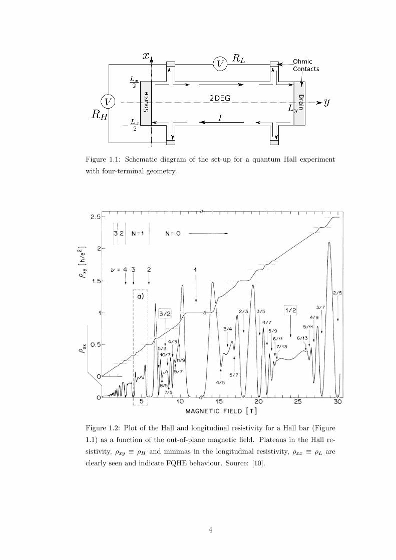
Figure 1.1: Schematic diagram of the set-up for a quantum Hall experiment
with four-terminal geometry.
Figure 1.2: Plot of the Hall and longitudinal resistivity for a Hall bar (Figure
1.1) as a function of the out-of-plane magnetic field. Plateaus in the Hall re-
sistivity, ρxy ≡ ρH and minimas in the longitudinal resistivity, ρxx ≡ ρL are
clearly seen and indicate FQHE behaviour. Source: [10].
4

1.1 Classical Hall Conductance
The effect of a voltage drop created across an electrical conductor when placed
in a magnetic field perpendicular to the direction of current flow has been known
since Hall’s discovery in 1879 [14]. Classical considerations alone are adequate to
describe this behaviour, which is attributed to the Lorentz force experienced by
the electrons inside the conductor. It will be shown in this section however that
classical considerations are not enough to predict the existence of Hall plateaus
for a two-dimensional conductor [15–17].
From the Drude theory of electrical conductivity [18], the average drift velocity of
an electron in an electric field E is
v = −eEτ0
m,
where τ0 is the mean free path time and −e, m are the charge and mass of the
electron respectively. The current density is
j = −nev = σ0E, (1.1)
where n is the electron density, σ0 = ne2τ0/m is the constant electrical conductivity
in the absence of a magnetic field. Including a magnetic field in the system in a
perpendicular direction to the electric field e.g., B = Bk, causes the motion of the
electron to be on the x− y plane and thus the conductivity and resistivity become
tensors σ and σ−1 = ρ respectively. Adding the Lorentz force to the force created
by the electric field (where it has been assumed that dv/dt = 0) gives
v = −e (E + v ×B)τ0
m. (1.2)
5

The above equation gives the x and y components of the drift velocity in terms of
the electric field components which can be substituted into (1.1) and rearranged
to give,
Ex = σ−10 jx + ωcσ
−10 τ0jy
Ey = −ωcσ−10 τ0jx + σ−1
0 jy,
where ωc = eB/m is the cyclotron frequency. Since E = ρj, the components for
the electric field above define the resistivity tensor to be,
ρ =
ρL ρH
−ρH ρL
=
σ−10 ωcσ
−10 τ0
−ωcσ−10 τ0 σ−1
0
. (1.3)
Components ρL and ρH are referred to the longitudinal and Hall resistivity respec-
tively. The conductivity is then easily extracted from (1.3) using σ = ρ−1.
σL =ρL
ρ2L + ρ2
H
=σ0
1 + ω2cτ
20
σH = − ρHρ2L + ρ2
H
= − ωcτ0σ0
1 + ω2cτ
20
= −neB
+σLωcτ0
(1.4)
From (1.4) it is noted that for a non-zero Hall resistivity, ρH 6= 0, the longitudinal
conductivity vanishes as the longitudinal resistivity vanishes. Thus in regions
where ρL vanishes, just as it is known to do in the QHE, the Hall conductance
tends to σH = −ne/B. In this regime where ρH 6= 0 but ρL → 0, the conductivity
and resistivity tensors become
σ =νe2
h
0 −1
1 0
, ρ =h
νe2
0 1
−1 0
. (1.5)
6

where ν = nh/(eB); this quantity is discussed in more detail in Section 1.2. To
make closer connections to the QH measurements in Figure 1.2, it would be con-
venient to transform resistivity values to resistances. For this a specific geometry
must be chosen and here a rectangular 2DEG is considered with length Ly in the
y-direction and Lx in the x-direction as shown in Figure 1.1. Resistivity is defined
as ρ = RA/W where A is the cross-sectional area perpendicular to the current
flow and W is the length over the voltage drop. Thus for this 2D, rectangular
system the result RH ≡ ρH is obtained and so the resistivity tensor in (1.5) is
equivalently the resistance tensor. In the QHE, ρL → 0 so then of course RL → 0
but for completeness, the relationship between the longitudinal resistance and the
longitudinal resistivity is ρL = RLLx/Ly.
According to this classical analysis, the Hall resistance should depend linearly on
the magnetic field and thus cannot predict the plateaus observed for the 2DEG
when it is placed in strong magnetic fields at low temperatures. To understand
how plateaus in the Hall resistance arise, a quantum treatment of an electron in a
magnetic field must be discussed.
1.2 Quantum Treatment of an Electron Subject
to a Magnetic Field
As already hinted in the introduction to this chapter, the IQHE lends itself to a
description of a two-dimensional (2D) system of electrons free from interactions.
This section will begin with an analysis of the behaviour of a single charged par-
ticle in a uniform magnetic field in the z-direction, from which the Landau level
spectrum can be derived. For simplicity a spin-less system is considered for which,
the Hamiltonian is given by
7

H =1
2m
(−i~∇− e
cA)2
, (1.6)
where −e and m are the charge and mass of the particle respectively and A is the
vector potential, related to the magnetic field via B = ∇×A. This Hamiltonian
can be solved using the Landau gauge, A = (0,−Bx, 0) where B is the magnitude
of the magnetic field [19]. With this particular choice of gauge there is no explicit
y-dependence in the Hamiltonian and thus the momentum in the y direction is
conserved [Py, H] = 0. This gives a plane wave solution for the y-dependence of
the wavefunction.
Ψ(x, y) = X(x)eikyy√Ly, (1.7)
where periodic boundary conditions have been assumed such that ky = 2πn/Ly
for some integer n and for Ly being the length of the system in the y-direction.
Substituting the solution Ψ(x, y) in the time independent Schrodinger equation
with Hamiltonian (1.6) gives the following eigenvalue equation for the x-coordinate
dependent part X(x), of the wavefunction
(− ~2
2m
∂2
∂x2+m
2ω2c
(x+ l2Bky
)2)X(x) = EX(x). (1.8)
The magnetic length lB is the natural length scale of the problem and ωc is the
cyclotron frequency which, corresponds to the minimum radius for the electrons
circular motion in the magnetic field. Their definitions are given below.
lB =
√~eB
ωc =eB
m(1.9)
8

From inspection it can be seen that the eigenvalue equation (1.8) is equivalent to
that of a one dimensional harmonic oscillator where l2Bky is the shifted position of
the center of the harmonic potential in the x-direction. Thus the energy spectrum
of the charged particle in a uniform magnetic field is given by
E =
(n+
1
2
)~ωc (1.10)
where n is some integer. Different values of n correspond to different Landau
levels, with the lowest Landau level (LLL) given by n = 0. Note that in the LLL,
the electron state is determined by a single quantum number, namely, the wave
vector ky. Solutions to (1.8) are given by
Xn(x) = Hn
(x+ l2Bky
lB
)exp
(−(x+ l2Bky)
2
2l2B
). (1.11)
It is straightforward to show that lB is the natural length scale of the system by
considering the correspondence between the x-coordinate at which the harmonic
oscillators in (1.8) are centered and the ky momentum values; i.e. x = −l2Bky =
−l2Bpy/~. By naively quantising this theory via py = −i~∂y, then the commutator
between the x and y coordinate is no longer zero, instead,
[x, y] = il2B.
Thus positions x and y cannot be simultaneously localised to an area smaller
than ∼ l2B near the centre of the one-dimensional harmonic oscillator. The area
corresponding to a single flux quantum and therefore to an electron is 2πl2B. The
Landau levels are highly degenerate and in fact for an infinitely long system,
the landau levels would be infinitely degenerate. This degeneracy is caused by
the continuous set of states for a free particle being compressed into a discrete
9

spectrum. To calculate this degeneracy, consider a system of length Ly in the
y-direction and Lx in the x-direction. The y-axis passes through the centre of the
system such that the y-directed edges intercept the x-axis at either ±Lx/2 (see
Figure 1.1). The largest possible momenta that an electron can occupy in the
ground-state is obviously the Fermi momenta ±kF . Thus the number of states per
Landau level (LL) ND is a sum of ky between the extremal values, since different
values of ky correspond to different states in a single Landau level.
ND =
kF∑k=−kF
1→ Ly2π
∫ kF
−kFdky =
LykFπ
, (1.12)
where the sum has been transformed into an integral over ky assuming Ly is large.
The extremal x-values are at the y-edges where x = ±Lx/2. From the harmonic
oscillator analysis, the relationship between x-space and momentum space ky is
x = −l2Bky and thus kF = Lx/(2l2B). This value for the Fermi momenta can be
substituted into (1.12). Using the form for the magnetic length given in (1.9) and
recognising that LxLyB is the total flux through the sample Φ and h/e is the
magnetic flux quantum Φ0 then
ND =Φ
Φ0
. (1.13)
Thus for each magnetic flux quantum penetrating the bar there is one state. Equa-
tion (1.13) allows the definition of another important quantity; the filling factor ν.
It corresponds to the ratio of the number of electrons N to the number of available
states ND.
ν =N
ND
(1.14)
This is the same number that appears in the equation for the Hall resistivity at a
10

given plateau and it corresponds to the number of states that are occupied. ν ∈ Z
corresponds to some integer number of completely filled Landau levels, whereas
ν = 1/3 means that only a third of all states in the LLL are occupied.
By solving the eigenvalue equation for the Hamiltonian (1.6) the energy spectrum
of the Landau levels have been derived for a single electron. These Landau levels
are highly degenerate and for an integer number of filled Landau levels there is a
gap of size ~ωc to the next available state. In the next section it will be discussed
how a slight modification to this LL spectrum can lead to the observed plateaus
in the Hall resistivity measurements for the IQHE.
1.3 The Integer Quantum Hall Effect
The focus of this section is to discuss the causes for the observed plateaus in the
Hall resistivity. The precise nature of how the Landau levels contribute to the
transport of current through the system is also reviewed. The arguments pre-
sented here are not rigorous but the mathematical details can be found in the
references given in this section.
Figure 1.3: Density of states for the first three Landau levels for; (a) a clean
system and (b) a dirty system containing impurities.
The 2DEG systems used in experiments are never completely free of impurities and
11

it turns out that it is these impurities that are essential to the observation of the
QHE. The impurities cause the LLs to broaden and lifts some of the degeneracy. In
turn the energy spectrum now consists of regions of extended states, in the centre
of the LL and localised states at the tails of the broadened energy spectrum,
see Figure 1.3. In QH experiments the Hall resistivity is measured as either the
magnetic field is varied or the carrier density is varied. In both cases, this effectively
means that the Fermi energy will change its position with respect to the Landau
level spectrum.
The plateaus in the Hall resistivity and/or Hall conductivity appear when the
Fermi energy is in a region of localised states, i.e. when some integer number
of Landau levels are completely full. In this region increasing the Fermi energy
only adds electrons to localised states and thus they make no difference to the
total Hall conductivity. Since the longitudinal conductivity is entirely dependent
on states at the Fermi energy [15], at a plateau the Fermi energy must lie in the
region of localised states for σL → 0. The Hall conductivity at a plateau, however
could be determined by considering only the extended states below the Fermi
energy. Laughlin [20] used the idea of this mobility gap between extended states
along with gauge invariance arguments to calculate the Hall conductance which
matched the experimental results.
Another important result used throughout this thesis which is applicable to both
the IQHE and the FQHE is that the current in the system is only transported
around the edges of the system and not through the bulk. This result was derived
by Halperin [21] who showed that when the electron density tends to zero, there
exists low-energy excited states which can transport current. Niu and Thouless
[22] calculated the electron propagator of the edge states of the QHE and showed
it was extended only in the direction along the edge and localized in all other
directions. At the edges or near an impurity LLs bend upwards due to a confining
potential that prevents electrons entering a forbidden region of space. Thus for
12

some cross-section of the 2DEG one would expect the energy profile to be similar
to that shown in Figure 1.4.
Figure 1.4: Energy levels of a 2DEG showing the first three LLs. The edges
of the 2DEG are at x = 0 and x = Lx. Two impurities are also shown in the
2DEG depicted by the shaded regions.
The LLs are full up to the Fermi energy and therefore there always exist at the
edges or around impurities extended states that support low energy excitations.
In the bulk, however, at a plateau, the Fermi energy lies only in the region of
localised states. Thus current is supported around the edges of a 2DEG or is
confined to some impurity and thus will not contribute to measurements of the
transport properties. This completes the brief review of the IQHE.
So far it has been shown to observe the QHE there must exist some mobility gap
which arises naturally in the 2DEG as a consequence of the applied magnetic field.
The mobility gap in the IQHE is the gap between extended states of the impurity-
broadened LLs. So far from this analysis there is no reason why plateaus should
exist at fractional values of filling factors. The remainder of this thesis is now
focused on the FQHE with the next section introducing the Laughlin wavefunction.
13

1.4 The Fractional Quantum Hall Effect and Laugh-
lin States
From experimental measurements of the Hall resistivity, the FQHE looks very
similar to the IQHE, the only difference being that the filling factor ν is a fraction.
However, the free fermion formalism that successfully predicts behaviours observed
for the IQHE fails for the FQHE. The reason for this is there is no energy gap
predicted within a given LL and so the FQHE is fundamentally very different to
the IQHE. The fact that the FQHE is observed only in cleaner samples, lower
temperatures and stronger magnetic fields [23] as compared to the IQHE suggests
that a mobility gap ∆ could be created by electron-electron interactions. The gap
∆ within a LL then plays a similar role to the cyclotron energy gap for the IQHE.
For the remainder of this section and for the majority of this thesis, only plateaus
in the Hall resistivity that correspond to the partially filled lowest Landau level
(LLL) are considered. In particular we are interested in filling factors of the form
ν = 1/m where m is an odd integer in this extreme quantum limit. When all
electrons occupy the LLL, the kinetic energy is fixed and only the Coulomb energy
and the effect of impurities need to be considered. So far there does not exist any
analytic wavefunction to solve the Hamiltonian with the 2D Coulomb interaction,
although it is possible to numerically compute the exact ground-state for a limited
number of particles using the method of diagonalistion [13].
Pioneering work for states with ν = 1/m was carried out by Laughlin and much
of the information reviewed here is from Laughlin’s work [13] and his discussion in
Ref. [23]. Laughlin postulated the idea of the formation of an incompressible fluid
which acts to stabilise the system at particular particle densities corresponding to
ν = 1/m. To produce an approximate ground-state wavefunction for this system
Laughlin used the reasoning; it must be anti-symmetric, reduce the amplitude
of finding two electrons close together which, consequently reduces the Coulomb
14

repulsion and also that the wavefunction must be an eigenstate of the total angular
momentum. The form of Laughlin’s wavefunction is;
ΨN =N∏i<j
(zi − zj)m exp
(−∑k
|zk|2
4l2B
), (1.15)
where the set {zi} are electron coordinates on the complex plane and N is the
total number of electrons in the system. The polynomial term (written above as
a product) is holomorphic and reduces the probability amplitude for finding two
electrons close together. Its power m must be an odd integer to keep the total
wavefunction anti-symmetric. The value of m appearing in the wavefunction will
be shown in the next section to be equivalent to the inverse filling factor, i.e.,
ν = 1/m. The wavefunction (1.15) describes a circular droplet of a 2DEG and
will be referred to as Laughlin’s wave function. The total angular momentum of
the state is mN(N − 1)~/2 and this value is proportional to the degree of the
polynomial in Eq. (1.15). The maximum angular momentum, ~lmax of a given
electron in the Laughlin droplet is given by the maximum power of a variable
in the polynomial, so for state (1.15), lmax = m(N − 1). Different values of l
correspond to different orbitals in the LLL, from observing the various powers of
the variables {zi}, only orbitals l = mk, where k is an integer from 0 to N − 1 are
occupied by electrons, the remaining orbitals are vacant.
It will be shown later in Section 1.6, that the radius of the quantum droplet fluid
described by (1.15) is dependent on the number of particles N and the number
of any quasiparticles or quasiholes inserted into the system. Thus the area of the
droplet cannot be altered without the injection or removal of particles from the
system. Systems behaving in this way are incompressible and there is a cost in
energy to add particles into the system. The fact that the Laughlin wavefunction
predicts the existence of some energy gap ∆ within the LLL, which is required to
observe plateaus in the Hall resistivity, lends support for Eq. (1.15) being a valid
15

microscopic representation of the FQHE.
Although Laughlin’s variational wavefunction is not an eigenstate of the exact
Hamiltonian, it has been shown to have a large overlap with the exact eigenstate
for a limited number of particles where the Coulomb Hamiltonian can be diag-
onalised numerically. Laughlin states are however an exact ground state for a
similar two-particle interaction Hamiltonian known as Haldane pseudo-potentials
[24] which will be discussed in more detail in Chapter 3. A powerful observa-
tion that Laughlin made about the wavefunction (1.15) was that it showed strong
similarities to the system for a one component plasma. This analogy is responsi-
ble for many interesting predictions about the FQH system and this idea will be
developed in the next section.
1.4.1 Analogy Between the Laughlin State and the One-
Component Plasma
From statistical mechanics, the local density at a given position r is
〈ρ (r)〉 =N∫dr2....drNZ (r, r2, ....., rN)∫
dr1....drNZ (r1, r2, ....., rN), (1.16)
where Z (r1, r2, ....., rN) is the partition function and the density operator is given
by ρ(r) =∑δ(r − ri). The partition function may be written in terms of the
potential ε as
Z (r1, r2, ....., rN) = eβε. (1.17)
Using the Laughlin wavefunction one can calculate the local density at a given
point z for the lowest Landau Level.
16

〈ρ(z)〉 =
Ne− |z|
2
2l2B
∫ N∏i=2
(d2zie
− |zi|2
2l2B |z − zi|2m
)N∏
i=2≤j
|zi − zj|2m
∫ N∏i=1
(d2zie
− |zi|2
2l2B
)N∏i≤j
|zi − zj|2m(1.18)
Requiring the quantum mechanical result be equivalent to the statistical result,
we must have
βε = m
(N∑i<j
ln |zi − zj|2 +N∑n=1
W (zn)
), (1.19)
where
W (z) = − |z|2
2ml2B. (1.20)
Here ε has the form of a potential that describes a one component, two dimensional
plasma [25]. The first term in the above expression is the interaction potential
between the charged particles whilst the second term is the background potential.
Defining β = −m, m is therefore inversely proportional to the temperature. From
the theory of plasmas, at small temperatures (corresponding to large m) plasmas
are known to crystallize and their is evidence of a phase change for the Laughlin
quantum fluid to a Wigner crystal at filling factors ν ≤ 1/7 [26]. Knowledge of the
behaviour of plasmas can be exploited to help described the FQHE phenomenon
for ν > 1/7.
If ρ0 denotes the equilibrium configuration of charges then the maximum energy
can be found from
17

∂ε
∂zi=
N∑j=1, 6=i
1
zi − zj+
∂
∂ziW (zi) = 0. (1.21)
In the continuum limit for large N values, this reads as
∂
∂z(Φ0(z)−W (z)) , (1.22)
where Φ0 is the Coulomb potential for the equilibrium charge distribution which,
is given in the large N limit by
Φ0(z) = −∫
d2ζ ln |z − ζ|2ρ0(ζ). (1.23)
Applying partial differentiation with respect to z to Eq. (1.22) gives a simple
equation for calculating the equilibrium density using the background potential
W (z).
∆W (z) = ∆Φ0(z) = −4πρ(z), (1.24)
where in the final expression of Eq. (1.24) Poisson’s equation has been used.
Therefore by calculating the Laplacian (∆ = 4∂z∂z) of the background potential,
the equilibrium density of charges can be calculated in the large N limit.
ρ(z) = − 1
4π∆W (z) =
1
2πml2B(1.25)
Using the above expression for density one can show that Laughlin states actually
correspond to filling factors ν = 1/m. It was shown previously in the chapter
that the degeneracy per Landau level is ND = Φ/Φ0; thus for each magnetic flux
18

quantum penetrating the sample there is a single state. Since ND/A = 1/(2πl2B),
where A is area of the sample, the filling factor from Eq. (1.14) is ν = N/ND =
2πl2Bρ = 1/m.
Laughlin’s plasma analogy has also been used to make interesting predictions about
the nature of the quasiparticles that arise from the system described by Eq. (1.15),
which are the subject of the next section.
1.4.2 Laughlin Excitations
The one-component plasma (OCP) analogy introduced in the previous section
provides an ideal setting for an investigation into the type of excitations that are
supported by the Laughlin state. The arguments presented here can be found
in Ref. [13]. Imagine that our FQH system is disk-shaped with a hole in the
centre through which an infinitely long solenoid is inserted such that the flux in
the conductor can be varied without altering the magnetic field. Through this
solenoid a single flux quantum is passed adiabatically. The result of this process
is that the Hamiltonian describing the system with the extra flux quantum added
H ′ differs from the original Hamiltonian H via a gauge transformation. Therefore
using a suitable gauge transformation, one can obtain an exact excited state of
the original H after the quantum flux was added to the system. Thus the excited
state corresponds to the creation of a quasiparticle or quasihole depending on the
sign of the quantum flux. Adding the quantum flux to the system (first consider
the quantum flux to be positive) must increase the outermost Landau orbital, l by
1. Therefore the maximum l-value of the system is now (N − 1)m+ 1 rather than
(N − 1)m. This new state satisfying the above properties can be written as,
Ψ+z0m =
N∏i=1
(zi − z0)Ψm (z1, z2, ...., zN) . (1.26)
19

I.e., The new state is the Laughlin state multiplied by the product of the difference
between the original particle coordinates zi and the position of the solenoid z0 (the
position where the solenoid pierces the quantum liquid has been generalised to any
position z0 rather than just at the origin). Since 〈Ψ+z0m |
∑i δ(zi − z0)|Ψ+z0
m 〉 = 0,
there is a zero probability of finding a particle at z0 and thus it is concluded that
we have created a quasihole at this position. Equation (1.26) can be generalised
for the creation of M quasiholes at positions w1, ..., wM via the above reasoning
as,
Ψ+w1,..,+wMm =
N∏i=1
M∏j
(zi − wj)Ψm (z1, z2, ...., zN) . (1.27)
Using the analogy between the FQH system and the OCP, the charge of the quasi-
hole can be calculated as follows [15]. Writing the magnitude squared of the
wavefunction in (1.26) as an exponential of the potential, i.e.,
|Ψ+z0m |2 = eβε. (1.28)
The corresponding potential ε can be written in terms of the potential from the
Laughlin wavefunction ε (1.19) with an extra logarithmic term;
βε = 2mN∑i<j
ln |zi − zj|+ 2N∑k
ln |zk − z0| −N∑n
|zn|2
2. (1.29)
Again the above potential is that of a classical one component plasma; however
there is an extra charge positioned at z0 whose potential is weaker by a factor of
1/m compared to the potential of the existing charges in the plasma. Plasmas
behave as to keep the system electrically neutral wherever possible, and therefore
the system will attempt to neutralise the quasihole with an accumulation of 1/m
charge near z0. Elsewhere the charge density will remain unchanged and constant.
20

Since it is the electrons in the system which carry the real electric charge, the ac-
cumulation at z0 has a net charge of −e/m once the electron charge density cancels
with the uniform background density. Thus it is concluded that the quasihole at
z0 must have a charge −e/m where −e is the electron charge.
Changing the sign of the quantum flux added to the system via the solenoid will
thus create a quasiparticle and according to the reasoning above, the maximum
powers of the zj in the Laughlin wavefunction will decrease by a unit value. One
way in which this can be done is to apply ∂/∂zi to the polynomial part of the
wavefunction. To generalise to the creation of such a quasiparticle at the arbitrary
point z0, the resulting state is given by
Ψ−z0m =N∏i=1
(∂
∂zi− z0
l2M
)Ψm (z1, z2, ...., zN) . (1.30)
Since the quasihole created by the extra quantum flux added to the system has a
charge of−e/m, it can be concluded that the quasiparticle must have charge +e/m,
created when removing a quantum flux. Not only do Laughlin quasiparticles have
a fractional charge, but they also obey fractional statistics. This can be seen
from calculating the Berry phase when a single quasiparticle adiabatically encircles
a second quasiparticle in the system [27]. The statistical phase gain from this
transformation is given by 2πν, where ν is the filling factor. The Berry phase
is equivalent to a double exchange of the two quasiparticles; thus for a single
exchange the wavefunction gains the phase πν. The fact that this result does
not give a resulting Berry phase of simply 2π is intriguing since the result shows
that even though the original and the final systems of quasiparticles are identical,
the wavefunction has undergone a transformation. The reason for this is the
two-dimensional nature of the system, where the operation of exchanging two
particles twice over is not equivalent to an identity transformation as it is in three
or more dimensions. Imagine adiabatically transporting a quasiparticle around a
21

stationary, second quasiparticle. In three or more dimensions this path can be
continuously deformed into a point, thus the total phase gain by this operation
must be equal to 2π. In two dimensions, however, the path of the quasiparticle
around the stationary, second quasiparticle cannot be deformed to a point because
of the singularity of the stationary quasiparticle position in the plane. Thus the
phase gain does not necessarily have to be equal to 2π.
Particles obeying fractional statistics are referred to as anyons since the interchange
of two such particles can result in any change of phase. There has been success in
observing the fractional statistical behaviour of Laughlin-type quasiparticles in QH
bars using interference experiments [28, 29]. The fractional statistics of Laughlin
state quasiparticles is referred to as Abelian statistics and there is a proposal that
some quasiparticles in FQH states may actually obey the less-trivial non-Abelian
statistics.
Non-Abelian statistics is a consequence of states containing multiple quasiparticles
being topologically degenerate [30]. In such cases exchanging identical particles can
result in the wavefunction undergoing a unitary transformation between degenerate
ground-states. FQH bars with quasiparticles obeying non-Abelian statistics have
been proposed as a potential qubit for a topological quantum computer [31–35]
though actually observing the non-Abelian statistics in FQH systems has proved
more difficult than for the Abelian case. One possible non-Abelian QH state is the
Moore-Read Pfaffian state to describe e.g., ν = 5/2 [36, 37] which is a particular
example of a more general class of non-Abelian states, the Read-Rezayi states [38].
However, the Moore-Read Pfaffian state is not the only proposed ground-state for
the ν = 5/2 FQHE [39] and it has been proposed that interference experiments
(similar to those carried out for Abelian quasiparticle FQH states) should help
resolve the issue of its microscopic description [40]. So far there have been no clear
results from interference experiments with regards to this matter [41–44].
This section completes all the introductory material needed for a basic understand-
22

ing of Laughlin’s wavefunction and the one component plasma analogy. It will be
used continuously in this thesis as a microscopic representation of the FQH states
with filling factors ν = 1/m, where m is odd. In particular the Laughlin state
will be used as a base for computing transport properties microscopically for a
FQH device and in the next section key ideas involving transport properties of the
FQHE will be discussed.
1.5 Review of Literature Probing Transport Prop-
erties in the FQHE
The primary focus of this thesis is on the transport properties of the FQHE which,
since the bulk states are incompressible, are determined by the 1D edge states of
the system. In this section a short overview will be given on the current theoretical
understanding of the edge states in the FQHE as well as the compatibility of the
theory with experiments. The discussion here will provide a motivation for the
work completed in later chapters and is based on the introduction of the work by
this author and V. Cheianov [45].
The 1D edges states in the FQHE consist of interacting electrons for which the
Fermi liquid theory breaks down and it was first proposed by Wen [46] that they
should instead, be described by a chiral Luttinger liquid. A chiral Luttinger liquid
has the key feature of low-energy excitations being collective sound modes and
it can be shown that the system has a four-terminal Hall conductance given by
ν(e2/h) [46]. In chapter 3 the formalism for the chiral Luttinger liquid will be intro-
duced. It is a phenomenological theory useful for describing transport properties
of the FQHE which are readily accessible to experimental measurements.
More recently, a great amount of theoretical and experimental effort has focused on
the transport properties of FQH edge states when the charge carriers are faced with
23

a single, or multiple potential barriers and tunnelling is observed. There are two
equivalent methods to initiate tunnelling in a QH device. The most common from
an experimentalist’s point of view is by physically moving the edges closer together
at some point along a Hall bar, known as a quantum point contact (QPC). Such a
constriction can be achieved by placing metallic plates above the 2D electron gas
and applying a negative bias causing a local depletion of electrons. As a result edge
states are brought closer together causing a finite probability of inter edge back
scattering. The strength of this pinching effect on the edge states is determined
by the magnitude of the bias applied to the magnetic plates. For ideal systems,
the same tunnelling behaviour can be obtained from placing an impurity into the
bulk which also couples the edges and allows back scattering to occur. Realistically
using an impurity is a much cleaner method to observe backscattering since a QPC
can have adverse effects on the surrounding quantum Hall fluid due to electrostatic
reconstruction [47].
One of the first pieces of work concerned with tunnelling at a QPC was carried
out by Kane and Fisher [48–50] who investigated tunnelling at both a weak link
and a weak barrier in a conventional Luttinger liquid. Similar work was also
carried out by Furusaki and Nagaosa [51] and Moon et al. [52]. At a weak link
tunnelling will be dominated by electrons in the Luttinger liquid since, effectively
the liquid is split into two separate islands. For a weak barrier however it is
the excitations of the Luttinger liquid that tunnel. For the work carried out
by Kane and Fisher a perturbative approach for the tunnelling Hamiltonian was
used in conjunction with the renormalization group (RG) to discover which of the
tunnelling processes were relevant in both the strong and weak back scattering limit
and predictions were made about the tunnelling conductance and the zero-bias
peaks in I-V characteristics. The predictions about the Luttinger liquid behaviour
is in stark contrast to that of the non-interacting system, the Fermi liquid. Here,
unlike the non-interacting case, the width of the zero-bias peaks are temperature
dependent, and in particular the conductance away from the peak has a power law
24

temperature dependence where the exponent of the power law is the interaction
parameter (determining the strength of the interactions between electrons) of the
Luttinger liquid. The reason for the differences is of course down to the interactions
between the Fermions in 1D and thus observing such behaviour in a 1D channel
will be key in discovering systems that are strongly correlated, non-Fermi liquids.
The form of the tunnelling Hamiltonian used in all of the referenced works in this
section can be mapped onto the boundary sine-Gordon model [53] and consists
of operators that annihilate a charge carrier in one direction and create another
carrier traveling in the opposite direction at some barrier.
So far there is experimental agreement of non-Fermi liquid behaviour in the Laugh-
lin type edge states of a FQH device [54, 55] though the specific value of the power
of the temperature dependence of the tunnelling conductance is slightly off the
expected theoretical value [56]. Experiments measuring shot noise and interfer-
ence experiments (all making use of one or multiple point contacts) are predicted
to prove the existence of fractionally charged carriers in the edge states as well
as display their (Abelian or non-Abelian) fractional statistics. In particular it has
been predicted that for Laughlin type QH states, the back scattered current in
shot noise experiments should be proportional to the charge of the carriers [57]
given by e∗ = νe in the weak back scattering limit at zero temperature, where ν is
the filling fraction of the lowest Landau level. Experimental work has claimed to
have observed Laughlin type quasiparticles in such experiments [58, 59] though not
all of the work agrees that the shot noise measurement is dependent only on the
charge of the quasiparticles. It has been claimed that the specifics of the tunnelling
barrier as well as the energy regimes used in the experiment can effect the value
of the back scattered current. This would account for a deviance in the predicted
value of the quasiparticle charge in the very weak back scattering limit obtained
in some experiments [60]. In particular, the boundary sine-Gordon model for var-
ious test states has not been able to resolve which ground state provides a good
description for even denominator filling fractions such as ν = 5/2. Experiments
25

at quantum point contacts for the ν = 5/2 states which measure tunnelling noise
and tunnelling conductance give predictions for quasiparticle charge e∗ and the
tunnelling particles interaction parameter, g [61]. There is still no obvious match
to the theoretical predictions of the various candidate states for the edges in the
ν = 5/2 system [43] and even distinguishing whether the state should display
Abelian or non-Abelian statistics is not obvious [39]. This problem was briefly
mentioned in the previous section.
The RG approach by Kane and Fisher is based on a 1D lattice model and it is
assumed that the edge states of the FQHE will display similar behaviour so this
approach is frequently used as a base model for theoretical predictions on transport
properties of the FQHE. There are important differences between the Luttinger
liquid model used for the perturbative RG analysis by Kane and Fisher and the
FQH edge states. The electron field operators in the Luttinger liquid model can be
derived microscopically from the 1D Hamiltonian describing a system of interacting
electrons. It is not the same for the FQH edge states since in this case, the edge
states result from a two-dimensional system of electrons in a strong magnetic field,
thus the low-energy effective theory is obtained by projecting the FQH states onto
the space of low energy edge states. The perturbative RG approach that works so
well for the lattice model Luttinger liquid cannot be extended straightforwardly to
the FQH edge states since it relies on the fact that interactions between electrons
can be treated perturbatively. Switching off the electron-electron interactions in
the FQHE will result in a completely different system altogether. So how do these
differences affect the formulation of a chiral Luttinger liquid as compared to that
of a conventional Luttinger liquid?
It is already understood that the low energy projection of the edge states in the
FQHE do not display exactly the same behaviour as the Luttinger liquid. One
example is the low energy projection of the electron field operator. In the Luttinger
liquid the anti-commutation relation for two spatially separated electron fields is
26

given by a delta function, the same behaviour of similar fields in the edges states
of a FQH system is not observed. There is another issue with the locality of the
effective tunnelling Hamiltonian for a quasiparticle being transferred between two
disconnected edges in the system. In the FQHE the tunnelling Hamiltonian takes
a similar form to that of the tunnelling Hamiltonian in the conventional Luttinger
liquid, i.e., the operator consists of creating a particle in one of the QH edge states
and annihilating a particle in the opposing edge [52, 62]. Without the perturbative
RG analysis at our disposal for FQH states there is no guarantee that the effective
theory tunnelling operators will be local. For the Luttinger liquid model however,
local operators in the microscopic theory are guaranteed to remain local in the
effective theory using the Kadanoff coarse graining procedure.
The problem of the locality of the tunnelling Hamiltonian has been investigated for
a FQH system containing multiple quantum point contacts. It was observed that
the tunnelling operators at one of the QPC’s did not commute with the tunnelling
operator at a different QPC, independent on the magnitude of their spatial sepa-
ration [63]. To impose the expected locality to which the quasiparticle tunnelling
operators should adhere, the effective quasiparticle operators had additional Klein
factors included in their representation [63–69]. The addition of the Klein factors
adds an extra phase to the quasiparticle fields and it is reasoned that this is a sta-
tistical phase which is gained during a tunnelling event between two disconnected
edges. This statistical phase is a result of the fractional statistics obeyed by the
quasiparticles. Including Klein factors results in the effective quasiparticle tun-
nelling operators at two different QPC to commute with one another. Results on
observables such as tunnelling currents are greatly dependent on the inclusion of
these Klein factors (for example compare work by Law et al. [66] with Jonckheere
et al. [70]).
To conclude, the model used to describe tunnelling in the FQHE has not been
tested microscopically so far. The model is based on the work carried out on a
27

conventional Luttinger liquid system and there is no obvious reason that applying
this work to a chiral Luttinger liquid should provide a true representation of the
behaviour observed in the FQHE. Tunnelling between edge states in the FQHE
is therefore an interesting property to be studied, in particular, predictions made
by the tunnelling Hamiltonian should be tested microscopically. Original work
concerning this issue is presented in Chapter 4 of this thesis. The geometry of the
FQH device that will be used in both Chapter 3 and Chapter 4 is introduced in
the next section of this introduction.
1.6 Disk Geometry Fractional Quantum Hall De-
vice
The first few chapters of this thesis concentrate on a FQH system with a particular
type of geometry that is introduced in this section for later reference. The FQH
device of interest consists of a ring of Laughlin-type FQH fluid with filling factor
given by ν = 1/m where m is an odd integer. This FQH device is shown in
Figure 1.5. This geometry has been chosen due to its convenient ground state
wavefunction, which has axial symmetry. Experiments are typically performed
using a Hall bar geometry such as that shown in Figure 1.1, however the properties
of interest, discussed later in this thesis, are not affected by the choice between
the ring, or Hall bar geometry. The inner radius of the ring is labelled as RI
and the outer radius is given by RO. For convenience in later works, the domain
corresponding to the inside the ring (|z| < RI) is denoted by DI and the domain
which confines the charges (RI ≤ |z| ≤ RO) is denoted by DM .
To create the macroscopic hole occupying the domain DI , an integer number of
M quasiholes are inserted at the center of the droplet at the coordinate z = 0.
Including the M quasiholes means that the wavefunction describing this system,
28

Figure 1.5: Schematic diagram for the FQH device with disk geometry. Elec-
trons are confined to the domain DM on the complex plane and at the edges
of this domain there is a sharp decrease to zero in particle density. The radii
of the inner and outer edge of DM are given by RI and RO respectively. Inside
the domain DI a number M of quasiholes have been inserted at the coordinate
z = 0 to create the inside edge of the disk. Regions excluding the domains DM
and DI contain a vacuum.
from (1.26) is given by
ΨMN =
N∏i<j
(zi − zj)mN∏k
zMk e− |zk|
2
4l2B . (1.31)
For a ring of sufficiently large width, i.e. RO −RI >> lB, transport in the system
will be confined to the edges due to the bulk being incompressible. At the interfaces
of the domain DM with the vacuum domains, there will be a sharp decrease to
zero in particle density. The larger the number of electrons N inside domain DM ,
then the sharper the decrease to zero in particle density. For the work carried out
in this thesis, we will mainly be interested in the large N -limit where the density
can be considered as a constant throughout the bulk of the system. In the region
of the magnetic length of the radius of the FQH droplet there is an overshoot in
the magnitude of the particle density before it drops to zero. This is a consequence
29

of the electron-electron correlations in the FQH fluid [71, 72].
The size of the macroscopic hole in the center of the droplet will depend on the
number of quasiholes M inserted at the center of the complex plane. To obtain an
expression for RI in terms of M it is noted that if the area of the domain DI was
filled with electrons (rather than quasiholes), then one could fit πR2Iρ electrons
into this space. Since a quasihole has charge e∗ = e/m, then a single quasihole
is (1/m)’th of a missing electron and so the domain DI actually consists of M/m
missing electrons. Therefore πR2Iρ ≡ M/m which when using the value for the
electron density ρ = 1/(2πml2B) gives
RI = lB√
2M. (1.32)
A similar method can be used to find an expression for R0 in terms of the pa-
rameters appearing in wavefunction of the system. Inside the area πR20 there are
effectively N + (M/m) electron-type particles and so πR2Oρ ≡ N + (M/m) which
gives the magnitude of the outer radius of the ring to be
RO = lB√
2mN + 2M. (1.33)
These equations for the radius RI and RO show explicitly that system described
by Laughlin is indeed incompressible since altering the area of the droplet will
subsequently inject or remove electrons from the system. Altering the value of
M however still preserves the area of the quantum fluid since the quasiholes cor-
respond to low-energy excitations of the inner boundary. A detailed discussion
of the low-energy edge excitations is given in Chapter 3. Since we have used
ρ = 1/(2πml2B), the values for RI and RO are exact for the large N limit.
In this introduction both the IQHE and the FQHE have been described and in
30

particular the reasons for the observed plateaus in the resistivity measurements
have been explained. For the IQHE, a free electron system can be considered
where interactions between charges are completely disregarded. In this picture, the
energy spectrum is the gaped Landau level dispersion, which with the the presence
of impurities in the 2DEG provide an explanation for the resistivity plateaus. One
can only explain the plateaus in the FQHE however by using strongly correlated
electrons. These interactions between the charges result in an energy gap opening
up within the LL’s. These gaps caused by electron correlations then play a similar
role to the to the LL gaps in the IQHE.
The Laughlin wave function has also been introduced. This state provides a micro-
scopic wavefunction for FQH states occupying the LLL. The bulk of the quantum
fluid described by this state is incompressible; however low-energy excitations can
be created at the edge of the fluid. Such properties, and many others, can be
shown using the Laughlin plasma analogy. In Section 1.5 the importance of these
low-energy excitations was discussed with respect to measurements on the trans-
port properties of the FQHE. The concept of tunnelling across the bulk states was
also discussed and how there is a lack of a solvable, microscopic description of
this process in the FQHE. Original work completed with regards to the effective
theory description of tunnelling will be presented in Chapter 4, after operators in
the chiral Luttinger liquid theory have been derived in Chapter 3. A large part
of the original work presented in this thesis uses the Monte Carlo (MC) method.
This will be the subject of the next chapter.
31

Chapter 2
The Monte Carlo Method
A large amount of original work presented in this thesis uses the Monte Carlo
(MC) method. In this section the main ideas and processes of MC simulations
are introduced. Particular attention is paid as to how the method can be applied
for computing observables in the microscopic representation of FQH systems. The
MC technique has proved to be a powerful tool for studies concerning the one-
component plasma (OCP) [73–76]. Since the Laughlin states for the FQHE can
be represented in terms of the partition function of this plasma, naturally the MC
computations have been extended to calculate many observables such as particle
densities and excitation energies of the Laughlin wavefunction [71, 77, 78].
The main problem for analytically calculating observables for Laughlin states is
that we are interested in the thermodynamic limit of the FQH system which holds
for a large number of particles (N →∞). This means that to calculate expectation
values of a general operator, A for a Laughlin system, for example given by;
〈A〉 =
⟨N,M
∣∣∣A∣∣∣N,M⟩〈N,M |N,M〉
=
∫ N∏k=1
d2zkΨMN AΨM
N∫ N∏k=1
d2zk|ΨMN |2
, (2.1)
32

one must calculate a large number (2N) of integrals. In Eq. (2.1), ΨMN is the
wavefunction for the LLL with disk geometry originally stated in Eq. (1.31) and
ΨMN is its complex conjugate. For ν 6= 1, where ν is the filling factor, there is no
simplification one can make to calculate these integrals analytically and thus one
must look to numerical methods such as the Monte Carlo procedure [79].
Looking at the averages in Eq. (2.1), the computation process that is commonly
used to calculate averages with respect to some trial wavefunction is the variational
Monte Carlo method, first used in calculations by W. L. McMillan [80]. The
most straightforward description to discuss how the variational MC algorithm
can be implemented for FQH correlators is by substituting the plasma analogy
|ΨMN |2 = e−βE into Eq. (2.1) to give the following expression for the expectation
value of A.
〈A〉 =
∫ N∏k=1
d2zke−βEA
∫ N∏k=1
d2zke−βE
. (2.2)
The expression (2.2) is now in a form reminiscent of the familiar statistical av-
erages with the denominator being thought of as the partition function of the
system. Monte Carlo computations can provide an estimate for the expectation
value of A by sampling possible states at random from a probability distribution
p(z1, z2, ..., zN) to perform the average. From (2.2) one can see that the partition
function is a continuous function and thus there are an infinite number of states
to be averaged over. Averaging over an infinite number of states is numerically
impossible and one must provide a cutoff Λ to the number of states used in the
average. Introducing the cutoff will introduce some statistical errors, though for
now there is no better method to perform the calculation exactly. So suppose Λ
states {λ1, λ1, ...., λΛ} are chosen with probabilities {pλ1 , pλ2 , ...., pλΛ} respectively,
then the best estimate for 〈A〉 is now a discrete sum of the states λi rather than
33

an integral over the continuum of states,
AΛ =
Λ∑i=1
Aλip−1λie−βEλi
Λ∑j=1
p−1λje−βEλj
. (2.3)
The quantity AΛ is known as the estimator. For an accurate value for the esti-
mator AΛ one needs to include the states λi that give the largest contributions
to the sum in (2.3). This process is known as importance sampling. Physical
systems choose states to occupy according to the Boltzmann probability distribu-
tion, which states that the probability of the system occupying state λi is given by
pλi = Z−1e−βEλi . It therefore makes sense to use this probability distribution for
finding states which have the largest contribution to the estimator. Substituting
the Boltzmann probability distribution into (2.3) gives;
AΛ = Λ−1
Λ∑i=1
Aλi . (2.4)
The next step is to form an algorithm that generates states according to the
Boltzmann probabilities. This is done using the Markov process such that if the
system starts in some initial state, then after a long enough running time the
Markov process generates a succession of states for the system with probabilities
given by the Boltzmann distribution. The states generated in this process are
called the Markov chain of states.
To show how the Markov process works, one needs to define transition probabilities
P (λi → λj) that give the probability that the state λj will be the next state in
the Markov chain when the system is currently occupying state λi. Transition
probabilities have the following conditions imposed: (i) they do not vary over time
and (ii) they do not depend on the history of the Markov chain (i.e., the states
34

that the system has already passed through), they only depend of the current
state λi and the next possible state in the Markov chain, λj. (iii) The transition
probabilities must of course satisfy
∑j
P (λi → λj) = 1 (2.5)
such that they have the correct normalisation. This constraint guarantees that at
each step in the Markov chain the system will definitely be in some final state, even
if it is the same as the initial state. With the transition probabilities now defined,
the conditions placed on the Markov chain can now be discussed. These are the
condition of ergodicity (CoE) and the condition of detailed balance (CoDB). When
both of these conditions, described below, are imposed on the Markov chain then
it is guaranteed that once the process has been run for a sufficiently long time,
the equilibrium distribution of states being generated will match the Boltzmann
distribution.
1. Condition of ergodicity (CoE): It should always be possible to reach any other
state in the system from some initial state in a finite number of steps.
2. Condition of detailed balance (CoDB):
pλiP (λi → λj) = pλjP (λj → λi). (2.6)
By following the CoE, one makes sure that every state has a non-zero probabil-
ity of being accessed at some point in the Markov chain, just like the Boltzmann
probability is non-zero for all possible states for the system. The CoDB on the
other hand makes sure that the equilibrium distribution is in fact the Boltzmann
distribution as opposed to some other probability distribution. The equation (2.6)
comes from the fact that by the definition of a system in equilibrium, the proba-
35
bility for a transition into a state and out of that state must be equal. It is once
the system reaches equilibrium and the probability distribution matches that of
the Boltzmann distribution that measurements for the observable (for example,
AΛ in (2.3)) can be taken.
Using (2.6) and the fact that one wishes for a probability distribution equivalent
to Boltzmann distribution when the system reaches equilibrium, the transition
probabilities must satisfy
P (λi → λj)
P (λj → λi)=pλjpλi
= e−β(Eλj−Eλi ). (2.7)
The next question is how are the transition probabilities chosen? So far there
only exists a condition on the ratios of the transition probabilities and so they are
not uniquely determined. This question can be avoided altogether by introducing
acceptance ratios. Imagine that the transition probabilities are split into two parts
such that,
P (λi → λj) = g(λi → λj)A(λi → λj) (2.8)
and therefore Eq. (2.7) becomes
P (λi → λj)
P (λj → λi)=g(λi → λj)A(λi → λj)
g(λj → λi)A(λj → λi)= e−β(Eλj−Eλi ). (2.9)
The probabilities g(a → b) are called selection probabilities and A(a → b) are
called acceptance ratios. To see the benefits of this notation it is noted that (2.9)
is always satisfied for the same final and initial state (say, state λi), no matter
what the value is for P (λi → λi). Therefore there is freedom in choosing and
manipulating other transition probabilities P (λi → λj) if the value of P (λi → λi)
36

can be adjusted accordingly such that (2.5) still remains satisfied. Thus the idea
behind splitting the transition probability into the selection probability and the
acceptance ratio is that the selection probabilities are the probabilities that a
transition will happen from an initial state into a final state and the acceptance
ratios give the probability that the next generated state is accepted/rejected and
are chosen such that (2.9) is satisfied.
Ideally, the larger the values of the acceptance ratios the quicker the Markov
process will reach equilibrium since there will be more states sampled in a shorter
amount of time. Therefore the larger of the two acceptance ratios in (2.9) is
always set to unity, whilst the other is adjusted accordingly so that the equation
still remains satisfied.
So far the discussion has been quite general for an equilibrium Monte Carlo cal-
culation. At this point however there are a selection of choices one could use to
calculate the acceptance ratios; in this work all computations were carried out in
accordance with the Metropolis algorithm [81]. The algorithm is simply defined
by the choice of the selection probabilities and is one of the most simple and most
common algorithms used. For the Metropolis algorithm implemented in the work
in this thesis, the selection probabilities are all equal to one another, and for a
system of N electrons, like for our FQH system, they are given by
g(λi → λj) = N−1, ∀ i, j. (2.10)
The selection probabilities in the equation for detailed balance (2.9) now cancel
each other and all that is left is the ratio of the acceptance ratios,
A(λi → λj)
A(λj → λi)= e−β(Eλj−Eλi ). (2.11)
37
Recall that the optimal way to choose the acceptance ratios is to make the largest
of the two in (2.11) equal to unity, therefore in the Metropolis algorithm acceptance
ratios have the form,
A(λi → λj) =
e−β(Eλj−Eλi ) for Eλj − Eλi > 0
1 otherwise.(2.12)
Other choices of acceptance ratios in the Metropolis algorithm are discussed in
Ref. [82]. The acceptance ratios (2.12) are such that if the energy of the new
state λj is less than or equal to the energy of our initial state λi then the new
state will be accepted, otherwise the new state is accepted with the probability
equal to e−β(Eλj−Eλi ). To decide if a new state should be accepted with a non-unity
acceptance ratio, a random number r is generated such that 0 ≤ r < 1, then the
new state λj is accepted if and only if
r < A(λi → λj) = e−β(Eλj−Eλi ).
To be more specific about the algorithm used in this work in accordance with
the FQHE, the different states of the system correspond to different positions of
electrons on the complex plane. It has already been shown that the outer radius
of a Laughlin FQH system with N electrons and M quasiholes at position z = 0 is
given by RO =√
2mN + 2M , where m = 1/ν is the inverse filling factor, and the
inner radius is RI =√
2M . Therefore before the Metropolis algorithm is initiated,
the initial state of the system is chosen by randomly placing the electrons inside
the disk on the complex plane with inner and outer radius RI and RO. Since
in this implementation of the Metropolis algorithm the selection probabilities are
all equal, to choose a new state an electron is chosen at random and its position
is shifted. Whether this new state is accepted or rejected then depends on the
acceptance ratios and thus the differences in energies of the initial and final state
38

as described in Eq. (2.12).
The exact Boltzmann energies that are chosen for a system in the FQH state will
actually depend on what observable is being measured. For those that match the
form given by (2.1) the plasma analogy can be invoked so that
ZN =
∫ N∏i=1
d2zie−βE =
∫ N∏i=1
d2zi|Ψ|2, (2.13)
which gives the energy of some state defined by particle coordinates λi = {z1, z2, · · · , zN}
to be
βEλi =N∑i=1
(|zi|2− 2M ln |zi|
)− 2m
N∑i<j
ln |zi − zj|. (2.14)
If one goes from state λk = {z1, z2, · · · , zk, · · · , zN} to λ′k = {z1, z2, · · · , z′k, · · · , zN}
then the difference in the energy between the initial and final state will only depend
on the energy contribution from the k’th particle which is given by
Eλk(z) =|z|2
2− 2M ln |z| − 2m
N∑i=16=k
ln |z − zi|, (2.15)
where z is the position of the k’th electron in either the initial or final state.
Therefore acceptance ratios from (2.12) are given by
A(λk → λ′k) =
e−∆Ek for Eλ′k − Eλk > 0
1, otherwise(2.16)
where
39

∆Ek =1
2
(|z′k|2 − |zk|2
)+ 2M ln
(|zk||z′k|
)+ 2m
∑i=16=k
ln
(|zk − zi||z′k − zi|
). (2.17)
The difficult question to determine is just how much of a shift should be imposed
on the electrons position? Moving the electron by too small amount means that
the energy range of the selected states will be narrow and thus it could take a
long time to reach equilibrium. Too large a shift is also counter productive since it
may be impossible to ever reach the states that minimise the energy and thus the
condition of ergodicity would not be satisfied. For this work the following method
is used. If the initial position of the particle is z = u+ iv then its new position is
given by
z′ = u+K
(δu− 1
2
)+ i
(v +K
(δv − 1
2
))(2.18)
where δu and δv are random numbers satisfying 0 ≤ (δu, δv) < 1, and K is some
constant that depends on the particulars of the program. The parameter K is
chosen such that there are a sufficient number of states that are being accepted or
rejected. Notice that the −1/2 term allows for possible moves in all direction on
the complex plane from 0 to 2π. The condition of ergodicity is satisfied since it is
possible for any particle to reach any position given a long enough time, and thus
all states are accessible in this Markov chain from any initial state.
Taking measurements for each new state that is accepted is not very efficient since
the measured value will only change a small amount for each successive particle
move. Also subsequent configurations in the Markov chain will be highly correlated
since only one particle position has been altered. Therefore the process of choosing
a new state and either accepting/rejecting it is carried out some number n times
between each measurement. After taking enough measurements when the system
has reached equilibrium, the expectation value of the estimator can be calculated
40

via calculating the average value of all the computed measurements, as shown in
Eq. (2.4). Due to the cutoff restricting the sampling to a finite number of states,
there is always an error associated with the value of the estimator in a Monte Carlo
simulation. Recall in the notation used here, the number of states involved in the
average of the estimator in Eq. (2.4) is Λ. The more measurements taken the
smaller the error becomes and eventually if it were possible to include all states so
that Λ→∞ then AΛ → 〈A〉 where 〈A〉 is the exact value of the statistical average
of some observable A shown in (2.2). Errors are estimated from the simulation
by determining the variance of the measurements recorded on the observable A.
Since the variance of the sample of measurements is
S2Λ =
1
Λ
Λ∑i=1
(Ai − 〈A〉)2 , (2.19)
then the magnitude of the error is given by SΛ and scales with the square root
of the number of measurements taken√
Λ. Eq. (2.19) holds only if the sample
of measurements is uncorrelated. An empirical check to see if subsequent mea-
surements are indeed uncorrelated is to compute nS2Λ, where n is the number of
configurations sampled between successive measurements. If nS2Λ is independent
of n, then subsequent measurements Ai are uncorrelated [83].
In this chapter, the MC method has been introduced, showing how statistical av-
erages can be computed in accordance with the Metropolis algorithm. To compute
observables for Laughlin states in particular, one can invoke the plasma analogy
to obtain an effective Boltzmann probability distribution which allows statistical
averages to be performed. Original work using the MC method and in particular
the Metropolis algorithm as discussed in this chapter, will be presented in Chapter
3, Chapter 4 and Chapter 5.
41
Chapter 3
Edge Excitations in
Laughlin-Type States
This chapter is devoted to the representations of edge excitations in Laughlin’s
theory of FQH states with filling factors ν = 1/m, where m is an odd integer. To
begin, in Section 3.1 we introduce the microscopic formalism for the description
of edge states and show the difficulties experienced when working analytically
with this representation. This leads onto a phenomenological description of the
FQH edge states pioneered by Wen [46] who proposed that the edge states can be
described by a chiral Luttinger liquid which has many similarities to a conventional
Luttinger liquid. This will be the subject of Section 3.2. In the final section of this
chapter, original work is presented for the overlaps of Laughlin states supporting
low-energy edge excitations.
42

3.1 Microscopic Representation of Edge Excita-
tions
In the introductory chapter of this thesis, it was pointed out that the Laughlin
wavefunction was a zero energy eigenstate for a short range, two-particle inter-
action. It was originally shown by Haldane [84] that there are a whole range of
additional states that are also zero energy eigenstates of this type of interaction
and they can be generated by multiplying the Laughlin state by a symmetric poly-
nomial Pk(zi) of the electron coordinates. The same findings have also been found
for other short range interactions like U(r) = ∇2δ2(r) [85, 86]. In this section
we will follow the Haldane pseudopotential argument to show that in general any
holomorphic function of electron coordinates describes a Laughlin-type state in
the LLL and also that these states correspond to the addition of excitations to the
edge states of a Laughlin-type FQH droplet.
Haldane pseudopotentials vm are defined as the expectation value of some potential
V that is dependent only on the relative angular momentum m′ of a pair of par-
ticles. In the LLL the kinetic energy term can be neglected and one can write the
interaction part of the Hamiltonian in terms of these Haldane pseudopotentials,
V =∞∑
m′=0
∑i<j
vm′Pm′(ij), (3.1)
where Pm′(ij) is a projection operator which selects states of relative angular mo-
mentum m′. Angular momentum contributions come from the polynomial part of
Laughlin’s wavefunction, so for now work is carried out in the holomorphic repre-
sentation of Laughlin’s wavefunction, which for a FQH droplet (the disk geometry
will be returned to later) with filling factor ν = 1/m is given by
43

ΨN =N∏i<j
(zi − zj)m. (3.2)
The angular momentum operator in complex coordinates is given by zi∂zi . Ap-
plying this operator to the state (3.2) for all particle coordinates gives the total
angular momentum M0 = mN(N − 1)/2 in units of ~. From the polynomial in
(3.2) one can see that the minimum, relative angular momentum between any two
electrons is m = ν−1. Therefore if we define a short range interaction such that the
Haldane pseudopotentials are non-zero only for relative angular momentum values
less than m (vm′ = 0 for m′ ≥ m) then the Laughlin state (3.2) is a zero-energy
eigenstate to the Hamiltonian (3.1). According to this potential, there also exist
an excitation gap allowing the observation of the plateaus in the Hall resistivity.
If, for example, two particles are forced to have a relative angular momentum of
m′ = 1 instead of m, then there will be a cost of energy v1. The state in Eq. (3.2)
however, is not the only eigenstate of this potential and generally, the states
ΨkN = Pk(z1, z2, · · · , zN)ΨN (3.3)
all have zero eigenvalues of the Hamiltonian (3.1) where Pk({zi}) are symmetric
polynomials with k denoting the degree of the polynomial. An introduction to
symmetric polynomials is given in the Appendix A.1. If the total angular momen-
tum of the Laughlin state (3.2) is given by M0 = mN(N − 1)/2, then the total
angular momentum of the Laughlin state multiplied by a symmetric polynomial of
degree k is M = M0 + k; thus multiplying the Laughlin state by symmetric poly-
nomials increases the total angular momentum of the state via moving electrons
to higher angular momentum orbitals.
Any symmetric polynomial can be generated by the addition and/or the multipli-
cation of power sum polynomials which take the form Sn =∑N
i=1 zni . Power sum
44

polynomials therefore provide a good basis for the description of edge excitations.
The degree of the polynomial labelled as k in Eq. (3.3) determines the degeneracy
for the momentum eigenvalue M = M0 +k. It is given by the number of partitions
λ = {λ1, λ2, . . . , λN}, which have the same weight |λi| = λ1 +λ2 + · · ·+λN = k. A
partition, λ is a set of integers, λi, that are ordered in decreasing size; λ1 ≥ λ2 ≥
· · · ≥ λN . Partitions are described in more detail in Appendix A.1. For k = 0 and
k = 1 the degeneracy is 1 and for k = 2 the degeneracy is 2. The important point
to make here however, is that each unique partition has a one-to-one correspond
with the configurations of boson edge excitations in the system. Each partition
also corresponds to a unique symmetric polynomial. If we consider the power sum
polynomials as a representation of the microscopic states, then we see that Sk can
be thought of as a creation operator of the k’th orbital and k∂Sk as an annihila-
tion operator also acting on the k’th orbital. It can be shown that such ladder
operators follow bosonic algebra [87].
To highlight the points made so far, consider a state of the type shown in (3.3)
with the angular momentum contribution from the multiplication of the symmetric
polynomial given by k = 3. There are three unique partitions that satisfy |λ| = 3.
These are λ1 = {3, 0N−1}, λ2 = {2, 1, 0N−2} and λ3 = {1, 1, 1, 0N−3}. For a general
partition of the form λ = {λ1, λ2, . . . , λN} the configuration of edge excitations
can be extracted as follows; the number of integers with the value λk = 1 in
the partition corresponds to the number of excitations in the angular momentum
orbital l = 1, the number of integers of the value λk = 2 corresponds to the
number of excitations in the angular momentum orbital l = 2 and so on until
the maximum possible integer which is λk = N , corresponding to an excitation
in the angular momentum orbital l = N . According to the theory of symmetric
polynomials, there are only allowed N orbitals and thus this provides the maximum
angular momentum contribution of the edge excitations. For more details on the
reasoning for this statement, see Appendix A.2.
45

Back to the example for |λ| = 3, then the partition λ1 corresponds to a state
with a single excitations added to the l = 3 orbital, λ2 corresponds to the state
with a single edge excitation added to the l = 2 orbital and the l = 1 orbital, and
finally λ3 corresponds to the addition of three edge excitations to the l = 1 orbital.
The microscopic wave functions for these three degenerate states are generated by
multiplying the Laughlin state by a product of power sum polynomials of degree
corresponding to the integers in the partition. Therefore, for a general partition
of the form λ = {λ1, λ2, . . . , λN} the corresponding microscopic state is
Ψ =N∏k>0
Sλi
N∏i<j
(zi − zj), (3.4)
where Sλi =∑N
j=1 zλ1j and only non-zero integers are included from the partition
(λi 6= 0). For our example where |λ| = 3, the three degenerate states are
Ψ1 = S3
N∏i<j
(zi − zj)
Ψ2 = S2S1
N∏i<j
(zi − zj)
Ψ3 = S31
N∏i<j
(zi − zj) (3.5)
So far we have considered a simple Laughlin FQH droplet with a single edge. Now
the partition formalism will be extended to the two-edged, disk-shape geometry
described by the state
ΨMN =
N∏i<j
(zi − zj)mN∏n=1
zMn . (3.6)
The additional factor which creates the macroscopic hole at z = 0 is itself a
46

symmetric polynomial and as a consequence is also a zero-energy eigenstate of
the Hamiltonian (3.1). The total angular momentum for this state however is
M0 = NM + (mN(N − 1)/2). Excitations to the outer boundary of the fluid are
added in the same way as in (A.15). Excitations for the inner boundary however
are added by multiplying the state (3.6) by power sum polynomials of the inverse
variable 1/zi. So, for example, a state labelled in terms of the number of excitations
nk in the k’th orbital on the outer boundary and in terms of n−k, the number of
excitations in the k’th orbital on the inner boundary is
|{n±k}〉 =N∏i<j
(zi − zj)mN∏n=1
zMn∏k>0
Snkk Sn−k−k
=N∏i<j
(zi − zj)mN∏n=1
zMn∏k>0
(N∑i=1
zki
)nk ( N∑i=1
1
zki
)n−k
, (3.7)
where, to shorten notation the power sum polynomials of variables zi and z−1i have
been represented as
Sk =N∑i=1
zki
S−k =N∑i=1
1
zki
The angular momentum contribution from the inner boundary is therefore negative
(a result from the excitations being represented by power sum polynomials of the
inverse variable) as compared to the angular momentum from the outer boundary.
This sets a cutoff for the maximum number of boson momentum orbitals occupied
for the inner boundary. The magnitude of the maximum total angular momentum
allowed for the inner boundary excitations is NM , where N is the number of
47

electrons and M is the number of quasiholes inserted at the position z = 0. A
higher value than this result gives a total angular momentum of the system less
than the value of M0 = mN(N − 1)/2, which physically does not make sense.
Power sum polynomials of the inverse variable z−1i can then be converted into a
partition formalism for the inner boundary. Thus for a two-edge system one will
have two separate partitions, one for each edge. To calculate observables of the
system, it is first of all important to consider the overlap of two states;
⟨{n′±p} |{n±k}〉 =
∫ N∏n=1
d2zi|zi|2Me|zi|
2
2
N∏i<j
|zi − zj|2m
×∏k>0
Snkk Sn−k−k
∏p>0
Sn′pp S
n′−p−p . (3.8)
As far as this author is aware, there are no analytic solutions for such integrals in
the large N limit except in the free fermion case where m = 1. In the free fermion
case the problem becomes trivial since the overlap integrals can be represented as
a series of overlap of Schur functions which have known solutions. This process
is detailed in Appendix A.2. For m > 1, then the Vandermonde determinant is
replaced instead by some determinant to the power m, which is much more difficult
to work with since the Schur function technique can no longer be applied.
So far in this chapter we have introduced how edge excitations can be represented
microscopically and the difficulty with calculating expectation values of these ex-
cited states for filling factors ν < 1 in the large N limit has also been noted. The
calculation of expectation values however can be computed numerically using the
Monte Carlo technique introduced in Chapter 2. The next section of this chapter
will focus on a phenomenological theory of how edge excitations can be represented
in the edge states of Laughlin-type systems. This theory is a powerful tool used
to make many predictions about transport properties of the FQHE.
48

3.2 Phenomenological Theory Representation of
Edge Excitations
The phenomenological theory discussed here was originally conceived by Wen [46]
who described the edge states of a FQH system as a chiral Luttinger liquid. As
already hinted in the introduction of this thesis, the model for the edge states is
loosely based on the model of a conventional Luttinger liquid [88, 89], which was
originally formulated due to the break-down of Fermi liquid theory for interacting
fermions in one dimension. The Luttinger liquid model is exactly solvable using
the technique of bosonisation first introduced by Tomonaga [89] and extended
in other works [90–92]. The key to the solubility of the model is linearising the
dispersion about the Fermi energy which introduces massless Dirac fermions. The
bosonisation procedure then allows the Hamiltonian for a 1D system of interacting
fermions to be expressed as a system of non-interacting Bosons. The elementary
excitations of this model can then be considered as collective boson modes, a
similar result to what has been found in the microscopic picture presented in
Section 3.1. Fermion operators in the original theory can then be expressed in
terms of the Boson fields that describe the low-energy excitations of the system.
The most distinct property of a Luttinger liquid is the occurrence of power-law
behaviours, where the exponent is dependent on the type of interaction and the
geometry of the system. The chiral Luttinger liquid system of the FQH edges also
have this property except, as will be shown later in this chapter, the exponents
are now universal and dependent only on the filling factor ν of the state [93]. Due
to the chiral nature of the system and the universality of the power-law exponent,
the FQHE is one of the best systems for observing Luttinger liquid-like behaviour.
In the remainder of this chapter the formalism for the chiral Luttinger liquid
will be introduced. As discussed in Section 1.5 there are subtle differences in
the phenomenological theory of the chiral Luttinger liquid and the theory of the
49
conventional Luttinger liquid.
3.2.1 Chiral Luttinger Liquid Formalism
The formalism used here to describe the chiral Luttinger liquid is based on the
works [94, 95] in which operators are projected onto the subspace of edge exci-
tations in order to define the zero mode operators and Boson creation and anni-
hilation operators for quasiparticles. It was shown in the previous section that
microscopically, the edge excitations can be represented by power sum polyno-
mials of the variables zi for an excitation on the outer boundary, or z−1i on the
inner boundary. Again we consider a disk shape geometry for the FQH system as
shown in Figure 1.5. These edge excitations are small incompressible deformations
of the boundary and generally they can be described by a set of parameters; tk
for the outer boundary and t−k for the inner boundary. Consider the following
wavefunction;
Ψ = ΨMN
N∏k=1
emw(zk) =N∏i<j
(zi − zj)mN∏k=1
zMk e− |zk|
2
4l2B
+mw(zk)≡ |N,M, {t±k}〉 (3.9)
where,
w(z) =∑k>0
(tkz
k +t−kzk
). (3.10)
The bra-ket notation has been introduced here for later calculations. This wave-
function is identical to the Laughlin wavefunction for the ground state system of a
disk-type geometry except for the additional function w(z) in the exponent. Dif-
ferentiating the state Ψ with respect to t±k brings down a power sum polynomial
S±k from the function w(z) in the exponent. Thus the states |{n±k}〉 can be gen-
50

erated by Ψ in Eq. (3.9) by applying differential operators in accordance with the
angular momentum orbitals that are occupied.
|{n±k}〉 =∏k>0
Sn±k±k ΨM
N =∏k>0
1
mn±k
∂n±kΨ
∂tn±k±k
∣∣∣∣t±k=0
(3.11)
The normalisation coefficient of the wavefunction (3.9) is given by the square-root
of the tau function of analytic curves τ νN(t±k, t±k), which in the semi-classical limit
takes the form
∫ N∏i=1
d2z|Ψ|2 = τ νN(t±k, t±k)→ τ ν(N,M, t±k, t±k). (3.12)
where,
τ ν(N,M, t±k, t±k) = D(N,M)×
exp
{m∑k>0
kR2kO |tk|2 + k
|t−k|2
R2kI
+ kt−ktk + ktk t−k
}, (3.13)
andD(N,M) ≡ τ(N,M, t±k, t±k)|t±k=0 is a function independent of t± and t±. The
tau-function has been studied in detail [96] and in Appendix B.2 it is calculated
explicitly using a field theory approach. In general, the overlap for two states of
the form (3.9) in the large N -limit is given by
⟨N,M, t±k|N ′,M ′, t′±k
⟩= τ ν(N,M, t±k, t
′±k)δN,N ′δM,M ′ . (3.14)
where the Kronecker delta terms represents that states of different N and M
are orthogonal in the large N limit. With the tau-function known, along with
equations (3.11) and (3.12), the overlap of states describing different sets of bosonic
51

edge excitations can be calculated. For excitations constrained on either the outer
boundary or the inner boundary,
〈{n±k}|{n±p}〉 =∏k,p>0
1
mn±k+n±p
∂n±k+n±pτ ν(N,M, t±p, t′±k)
∂tn±k±k ∂t
n±p±p
∣∣∣∣∣t±k=0
= D(N,M)∏k>0
(kR±2k±
m2
)n±kn±k! δpk, (3.15)
where R− ≡ RI is the inner boundary radius and R+ ≡ R0 is the outer boundary
radius. The formula for the overlap of states was originally obtained by Cheianov
et al. [94] for a single edged FQH droplet. For this thesis the overlap formula
(3.15) has been extended to a two edged system for the disk geometry FQHE. In
Section 3.3, overlap integrals of states supporting low-energy edge excitations are
computed microscopically and compared to the predictions from Eq. (3.15).
As expected, such overlaps are reminiscent of bosonic algebra, thus our next step
is to define raising and lowering operators to act on the states as follows;
a†±p |n±p〉 =√n±p + 1 |n±p + 1〉 ,
a±p |n±p〉 =√n±p |n±p − 1〉 . (3.16)
In accordance with previous notation +p corresponds to a ladder operator acting
on the p bosonic mode of the outer boundary and −p corresponds to the same
value mode but on the inner boundary. Using (3.11) and (3.12), and choosing a
representation in terms of t±k as in [94], these operators take the form
52

ap =1
RpO
√mp
(∂
∂tp−mpt−p
), a†p = Rp
O
√mp tp.
a−p =RpI√mp
(∂
∂t−p−mptp
), a†−p =
√mp
RpI
t−p. (3.17)
The mixture of inner and outer boundary terms for the annihilation operators
(i.e. they contain both tp and t−p) is a consequence of the mixed inner and outer
boundary t±k in the tau-function (3.13). Even with the mixture of inner and
outer boundary terms, it is a straightforward calculation to show that operators on
opposing boundaries commute with each other [a±k, a†∓k] = 0 and the commutation
relations for operators acting on the same boundaries follow the usual bosonic
algebra [a±k, a†±p] = δpk. In the chiral Luttinger liquid theory, zero-mode operators
must also be defined. For the outer boundary these are denoted as θN which
extracts the number of particles from a state, and eiϕN which is its conjugate
operator. There also exist similar operators for the inner boundary θM and eiϕM
that act on the quasihole number M . Using the state notation introduced in (3.9);
eiϕN |N,M, {t±k}〉 = |N + 1,M, {t±k}〉 ,
θN |N,M, {t±k}〉 = N |N,M, {t±k}〉 ,
eiϕM |N,M, {t±k}〉 = |N,M + 1, {t±k}〉 ,
θM |N,M, {t±k}〉 = M |N,M, {t±k}〉 . (3.18)
These operators satisfy the commutation relations; [θx, eiϕy ] = eiϕxδx,y where x or
y = N or M . With objects defined in (3.17) and (3.18), we are now in a position
to construct bosonised forms of the fermion field operators. In this construction, it
is assumed that the edges are sufficiently far apart such that they are completely
independent of each other, thus one must define an electron operator for both
53

the outer boundary ψm,O and the inner boundary ψm,I . Only the outer boundary
operator ψm,O will be explicitly constructed, the method used is identical for the
inner boundary and so it will not be repeated. The final expression for ψm,I will
be stated at the end of the construction of ψm,O. Consider the matrix element
〈N,M, {t±k}|ψ†m,O(ζ)∣∣N ′,M ′, {t′±k}
⟩. (3.19)
Since the bosonic operators ap and a†p have been defined in terms of the t-representations,
rather than seeing the fermion operator ψ†m,O in (3.19) as a creation operator act-
ing on the state to the right, it can instead be thought of as an annihilation
operator acting on the left-state. This choice is convenient since from Laughlin’s
work discussed in the introductory chapter of this thesis, we know the microscopic
expression for a hole created in a Laughlin state is given by
〈N,M, {t±k}|ψ†m,O(ζ)∣∣N ′,M ′, {t′±k}
⟩= ζMe−
|ζ|24 emw(ζ)
×∫ N∏
i=1
d2zi(ζ − zi)mem(w(zi)+w(zi))|ΨMN |2δN,N ′+1δM,M ′ , (3.20)
where ΨMN is the ground state Laughlin wave function when no edge excitations
have been added to the system (see Eq. (1.31)) and the Kronecker delta terms
follow from (3.14). To project this operation on the low energy edge states, (3.20)
is expected to be equivalent to
〈N,M, {t±k}|ψ†m,O(ζ)∣∣N ′,M ′, {t′±k}
⟩= ψ†m,O(ζ)τ ν(t±k, t±k)δN,N ′δM,M ′ , (3.21)
where, in this representation ψ†m,O is now the effective, low energy electron opera-
54

tor. The aim of what follows is to manipulate (3.20) to be in the form (3.21) and
thus obtain an expression for the low-energy effective electron operator. Since the
fermion operator must act on the outer boundary, it is safe to assume ζ > zi so
the following expansion can be used in (3.20),
N∏i=1
(ζ − zi)m = ζmN exp
(m
N∑i=1
ln
(1− zi
ζ
))= ζmN exp
(−m
∑k>0
1
kζk
N∑i=1
zki
).
The sum over the coordinates zi in the exponent of the above expression has the
form of the power sum polynomial. It has already been discussed how power sum
polynomials can by extracted from states |N,M, {t±k}〉 by differentiating the state
with respect to tk (e.g., see Eq. (3.11)). Using this argument and Eq. (3.14) allows
the expression in (3.20) to be written as,
〈N,M, {t±k}|ψ†m,O(ζ)∣∣N ′,M ′, {t′±k}
⟩= ζmN+Me−
|ζ|24 emw(ζ)e
−∑k>0
1
kζk∂∂tk
×δN,N ′+1δM,M ′τν(N,M, {t±k}, {t′±k}).
(3.22)
The matrix element of ψ†m,O is now in a similar form to its effective, low energy
representation in (3.21); all that remains is to sort out the zero-mode parts of the
operator. According to (3.18), the zero mode operators appear in the effective
field representation of the electron operator as a consequence of the following
contributions:
ζmN+M → ζmθN+θM ,
δN,N ′+1 → eiϕN δN,N ′ .
55
To finish the calculation, the final expression for the electron effective field operator
is expressed in terms of the boson ladder operators ap and a†p using (3.17), since
this representation is the most familiar and easy to work with as compared to the
t-representation. Our electron field operator is thus,
ψ†m,O(ξ) = eiϕN emφO(ξ), (3.23)
where φO is the bosonised part of the operator given by
φO(ξ) = −iξR
(θN +θMm
) +∑k>0
√1
mk
(e−ik
ξRa†k − e
ik ξRak
)= φ0
O(ξ) + φ+O(ξ) + φ−O(ξ), (3.24)
where we have decomposed the field φO in terms of its zero mode contribution
φ0O, its creation operator part φ+
O and its annihilation operator part φ−O. This
notation will be used to shorten expressions in later calculations. It is noted that
a non-trivial coordinate transformation has been made in Eqs. (3.23) and (3.24).
The coordinate ξ is now the longitudinal coordinate along the edges of the system
where ξ ∈ [0, 2πR] and R is the radius of the ring of FQH fluid. This is because
in the effective theory of edge states we assume that the edge states are one-
dimensional. As a consequence, terms in (3.23) that are dependent only on the
transverse direction to the ring of fluid (such as e−|ξ|2
4 ) have also been dropped.
Conjugating the field the field ψ†m,O(ξ) gives the bosonised representation of the
electron annihilation operator,
ψm,O(ξ) = e−mφO(ζ)e−iϕN , (3.25)
56

where φ0(ξ) is given in (3.24). In general one can write the bosonisation formulae
for general field operators ψp,O in the low-energy effective theory, where p is some
integer. The operator ψp,0 corresponds to the annihilation operator of particle with
charge e∗ = (p/m)e in the Laughlin state ν = (1/m). Therefore ψp=1,O corresponds
to the field for a single Laughlin quasiparticle with charge e∗ = (1/m)e = ν−1e
and ψp=m,O corresponds to the field describing m quasiparticles, or equivalently a
single electron. These general operators for the outer boundary take the form
ψ†p,O(ξ) = eipmϕN epφO(ξ),
ψp,O(ξ) = e−pφO(ξ)e−ipmϕN . (3.26)
Carrying out an equivalent calculation as shown here but now for the inner bound-
ary, the field operators ψp,I , ψ†p,I corresponding to creating or annihilating a particle
of charge e∗ = (p/m)e respectively are given by
ψ†p,I(ξ) = eipmϕN eipϕM epφI(ξ),
ψp,I(ξ) = e−pφI(ξ)e−ipmϕN e−ipϕM , (3.27)
where now the boson field φI(ξ) takes the form
φI(ξ) = − iξ
mRtM +
∑k>0
√1
mk
(eik
ξRa†−k − e
−ik ξRa−k
)= φ0
I(ξ) + φ+I (ξ) + φ−I (ξ). (3.28)
Similar to the outer boundary Bose field, the inner boundary boson field has
57
been decomposed in terms of the zero mode part φ0I , creation part φ+
I and the
annihilation part φ−I . What is missing from our discussion so far is the convention
of the ordering of the fermion fields. In fact this is a difficult point to comment
on because changing the type of operator ordering used alters the normalisation
coefficient of the fields. Without any microscopic calculations to compare to, the
normalisation coefficient cannot be determined in this theory alone. This problem
will be analysed in detail in Chapter 4, for now we define the ordering of the
operators to be
eφX(ξ) = eφ0X(ξ)eφ
+X(ξ)e−φ
−X(ξ)e
12
[φ+X(ξ),φ−X(ξ)], (3.29)
whereX = I/O and the following commutation relations have been used [φ0X , φ
+X ] =
[φ0X , φ
−X ] = 0. The commutation relation for the operators φ+
X and φ−X is given by,
[φ+X(ξ), φ−X(ξ)
]=∑k,p>0
[a†±k, a±p]
m√pk
= −∑k>0
1
mk. (3.30)
To complete the calculation the sum over k needs to be performed. There are two
natural cutoffs that can be considered for the low-energy limit of the system. The
first is related to the breakdown of the Boson creation and annihilation operators
in the Luttinger liquid theory, which are only independent operators for k ≤ N ,
this cutoff is a consequence of the theory of symmetric polynomials mentioned in
the previous section of this chapter. Therefore N could be a valid cutoff for the
sum. However there is also an obvious limit on the energy of the edge excitations
which is related to the bulk energy gap. If quasiparticles have an energy larger
than the bulk gap energy ∆ then they are able to travel through the bulk de-
stroying the representation of the chiral Luttinger liquid edge states in the FQHE.
The dispersion relation for the Bose excitations is linear at the edge and so the
maximum momentum for a quasiparticle is p = ∆/v where v is the quasiparticle
58

velocity. The momentum corresponding to a given edge orbital k is also given by
p = ~k/R and therefore the maximum value of the orbital according to the bulk
energy gap is k ≤ R∆/(v~) ≡ Λ. The value of the radius R is on the order of N
in the large N limit. Thus the two cutoffs are essentially equivalent. In this work
we use Λ ∼ R as the cutoff, which has a more apparent meaning in terms of the
physics of the system.
The sum over k in (3.31) is performed using Λ ∼ R ≡ |b| as a soft cutoff such that∑k>0 k
−1 →∑
k>0 k−1e−k/R = − ln(1− e−1/R). Therefore,
[φ+X(ξ), φ−X(ξ)
]= − 1
mln(1− e−1/R). (3.31)
The result in (3.31) only holds when the variable of the two boson fields is the
same. It is because of the form of the commutators of the boson fields such as
(3.31) that power law behaviours are observed in the transport properties of the
FQHE. For an example see Chapter 4, where matrix elements are calculated for
particles tunnelling across the bulk of a FQH device. The exponent of the power
law for Laughlin state FQH systems is related to m which is a universal parameter
defined from the bulk states of the system.
The Hamiltonian for this system is then equivalent to the Hamiltonian for a con-
ventional Luttinger liquid except the charge carriers move only in one direction, as
imposed by the magnetic field acting on the system. In terms of the boson fields,
the Hamiltonian for the chiral Luttinger liquid describing both the inner and outer
boundary edge states is
H = ~v∫ 2πR
0
dx[(∂xφI(x))2 + (∂xφO(x))2] (3.32)
where v is the velocity of the inner and outer boundary edge excitations. In this
59

chapter both the microscopic representation and the phenomenological descrip-
tion of the edge states has been presented. In the microscopic picture it has been
shown that the edge excitations can be added to the system by multiplying Laugh-
lin’s wavefunction by a symmetric polynomial. Such new states are zero energy
eigenstates of a short-range interaction Hamiltonian, however the total angular
momentum is changed and depends on the configuration of the excitations at the
FQH droplet boundaries. The phenomenological approach based on the work by
Wen shows how the edge states of the FQHE have close behaviour to a conven-
tional Luttinger liquid and allows predictions to be made on transport properties
of the FQHE. As discussed in the introductory chapter to this thesis, there is work
supporting this theory and the Luttinger liquid-like behaviour of the edge states.
The next, and final section of this chapter presents computations for overlaps of
Laughlin states supporting edge excitations, from a microscopic perspective.
3.3 Numerical Verification of Analytic Formulas
for Overlap Integrals
In this section, numerical data will be presented for the overlap integrals of states
containing both inner and outer boundary edge excitations. The overlap integrals
in the microscopic picture are computed using the MC method. This work validates
the analytic formula for the overlap integrals originally obtained in the work by
Cheianov et al. for a single edge FQH droplet [94]. In Section 3.2 the formula was
extended to include two edges in the FQH droplet as depicted in Figure 1.5. The
equation is restated below for convenience.
〈{n±k}|{n±p}〉 =∏k,p>0
1
mn±k+n±p
∂n±k+n±pτ ν(N,M, t±p, t′±k)
∂tn±k±k ∂t
n±p±p
∣∣∣∣∣t±k=0
, (3.33)
60

where R− ≡ RI is the inner boundary radius and R+ ≡ R0 is the outer boundary
radius and,
τ(N,M, t±k, t±k) = D(N,M)×
exp
{m∑k>0
kR2kO |tk|2 + k
|t−k|2
R2kI
+ kt−ktk + ktk t−k
},
(3.34)
is calculated explicitly in Appendix B. The function,
D(N,M) ≡ τ(N,M, t±k, t±k)|t±k=0 (3.35)
is independent of t±k and t±k and will be referred to as the zero mode part. The
microscopic computation of the overlap of states is important for two reasons.
Firstly, it provides a good test of the MC method for computing observables in
the FQHE. Secondly, the microscopic computations provide a good method to
check the form of the tau-function. See Appendix B for more details.
There are an infinite number of possible configurations of the boson occupied
orbitals {n±k}. Since it is an impossible task to verify all states satisfy the analytic
formula for the overlap integrals, the test is carried out for states satisfying the
total edge state contribution to the orbital angular momentum of |lI | = 0, or
|lI | = 2 for the inner boundary and lO = 0 or lO = 2 for the outer boundary. With
this angular momentum cutoff, the highest possible orbital that can be occupied
corresponds to the power sum polynomial S±2 with a single excitation. Therefore,
to perform the microscopic computations using the MC method, we seek states of
the form,
61
|n−1n−2n1n2〉 =
[N∑k=1
1
zk
]n−1[
N∑k=1
1
z2k
]n−2[
N∑k=1
zk
]n1[
N∑k=1
z2k
]n2
×N∏i<j
(zi − zj)mN∏i=1
zMi e− |zi|
2
4
=2∏
k=−2
Snkk
N∏i<j
(zi − zj)mN∏i=1
zMi , (3.36)
which has been obtained from Eq. (3.6) from Section 3.1. All possible states using
the notation in (3.36) are given in the left-hand column of Table 3.1, excluding
the trivial case 〈0|0〉. These combinations of states were obtained using |lI | =
n−1 + 2n−2 = 2 or 0 and lO = n1 + 2n2 = 2 or 0 for the total angular momentum
contribution for the inner and outer boundaries, respectively. More information
related to the array of states that correspond to certain angular momentum values
is given in Appendix A. The overlap integrals for the states given in Eq. (3.36)
are difficult to calculate in the large N limit for m 6= 1, as discussed in Section
3.1. Therefore to check the analytic formula for the overlap integrals given in
(3.34), the MC method is used. The MC method works by calculating statistical
averages and therefore ratios of the overlaps of states are computed which have
the following form,
⟨n′−1n
′−2n
′1n′2|n−1n−2n1n2
⟩〈0|0〉
=
∫N
|ΨMN |2
2∏p=−2
Sn′pp
2∏k=−2
Snkk∫N
|ΨMN |2
, (3.37)
where the following shorthand notation has been used:∫N≡∫ ∏N
i=1 d2zi and ΨMN
is the Laughlin wave function for the disk geometry FQH fluid. In total there are 8
states that correspond to the angular momentum cutoffs that have been imposed.
This results in a total of 8× 8 MC simulations run to compute overlap integrals of
the form (3.37). The overlaps were calculated for a system with N = 60 electrons
62

in the quantum fluid and M = 56 quasiholes in the center of the droplet to create
the inner boundary of the system. To compute the overlap integrals, FQH systems
were chosen that correspond to the filling factor ν = m−1 = 1/3.
All off-diagonal overlap integrals (i.e., where the occupation numbers in the left
state were different to those in the right state) were decreasing in magnitude as
compared to the diagonal elements and thus these results are not listed here. It
is noted however that the analytic expression for the overlap integrals (3.33) also
predicts zero for these off-diagonal elements in the large system size limit. The
results for the diagonal overlap integrals have been listed in Table 3.1 along with
the corresponding analytic values predicted by Eq.(3.33).
According to the analytic expression for the overlap integrals, all results will be
proportional to the zero-mode part of the tau-function, D(N,M). The form of
this function is unknown and therefore results in each of the rows listed in Table
3.1 correspond to ratios of overlap integrals of the form
〈2000|2000〉〈n−1n−2n1n2|n−1n−2n1n2〉
, (3.38)
where the denominator corresponds to the state listed in the left-hand column of
Table 3.1.
It is clear that the MC data in Table 3.1 is in complete agreement with the an-
alytic expression for the overlap integrals, originally derived by Cheianov et al.
This is something that has never been microscopically checked before. The results
also show that the form of the tau-function calculated in Appendix B accurately
represents bosonic excitations contained in the microscopic states. In this section
it has been shown that the MC method is a useful tool for performing micro-
scopic computations for Laughlin type systems for large system sizes. The overlap
integrals in Eq. (3.37) were straightforward integrals for the MC method to han-
63

〈n−1n−2n1n2|n−1n−2n1n2〉 Analytic prediction MC Result
〈2000|2000〉 1.00 1.00± 0.02〈0100|0100〉 0.333 0.333± 0.006〈2020|2020〉 1.01× 10⁻⁵ (1.05± 0.05)× 10−5
〈2001|2001〉 6.7× 10⁻⁶ (6.8± 0.2)× 10−6
〈0120|0120〉 6.7× 10⁻⁶ (6.7± 0.2)× 10−6
〈0101|0101〉 2.2× 10⁻⁶ (2.1± 0.1)× 10−6
〈0020|0020〉 3.58× 10⁻¹⁰ (3.55± 0.09)× 10−10
〈0001|0001〉 1.19× 10⁻¹⁰ (1.19± 0.03)× 10−10
Table 3.1: This table compares the analytic predictions for the overlap of states
containing edge excitations on the inner and outer boundary of a two-edged
FQHE. The second column lists the analytic predictions for the ratio of the
overlap 〈2000|2000〉 with the overlap integral shown in the first column of the
table. The third column lists the MC data for the same ratio of integrals.
dle. In the remaining chapters of this thesis the MC method will be applied for
more complicated computations in the microscopic theory of Laughlin-type FQH
systems.
64

Chapter 4
Zero-Mode Tunnelling Matrix
Elements
From the discussion in the introductory chapter of this thesis, tunnelling mea-
surements are an important transport property to observe and test the Luttinger
liquid-like behaviour of the FQHE. The theoretical description of tunnelling uses
the phenomenological theory of edge states proposed by Wen to create an effective
tunnelling Hamiltonian which is analysed by using a renormalization group (RG)
approach [52]. However since there are no microscopic calculations to compare the
calculations to, there are questions about how accurate a description this is. The
question which we would like to answer in this chapter is whether the effective
tunnelling Hamiltonian makes predictions that can be verified microscopically?
Also, is the tunnelling Hamiltonian a local operator? The RG analysis provides
flow equations for the tunnelling parameters; however without any initial condi-
tions from a microscopic model with which to compare, the flow equations cannot
provide answers to questions such as at which scales certain tunnelling processes
become irrelevant? To investigate these problems a microscopic model for tun-
nelling between edge states using the geometry of the FQH disk shown in Figure
1.5 is developed. It has already been discussed in Chapter 3 that in the micro-
scopic theory the matrix elements of Laughlin states cannot be solved analytically
65

by any methods known to this author and therefore tunnelling matrix elements
will be computed numerically using the MC method.
The microscopic tunnelling matrix elements can then be compared to the effec-
tive theory predictions where the tunnelling Hamiltonian is constructed using the
bosonised operator formalism introduced in Section 3.2 of Chapter 3. Only the
simplest possible matrix elements are considered initially; these are referred to as
the zero mode matrix elements and correspond to a system absent of any low-
energy boundary excitations in the FQH device. The computations presented in
this chapter are based on work by this author and V. Cheianov [45].
To begin, the representation of the zero mode tunnelling matrix elements is given
for the microscopic theory. Also in Section 4.1 the methods of calculating the
tunnelling matrix elements using MC are discussed. In Section 4.2 the low-energy
projection of the tunnelling Hamiltonian matrix elements are derived using the
bosonised formulae for the fermion operators derived in Chapter 3. In the Section
4.3 a comparison is made between the effective theory predictions and the mi-
croscopic calculations for the size dependence of the tunnelling matrix elements.
The final section presents a conclusion and summary for the work covered in this
chapter.
4.1 Microscopic Computation of the Zero Mode
Tunnelling Matrix Elements
In this chapter, only FQH states occupying the lowest Landau level are considered.
Since the exact ground state of a FQH system is not known, we instead use the
Laughlin wavefunction. To consider tunnelling across the bulk of a FQH device,
a disk-shaped Laughlin system is used consisting of an inner and outer edge as
shown in Figure 4.1. To create a second edge in our system such that tunnelling
66
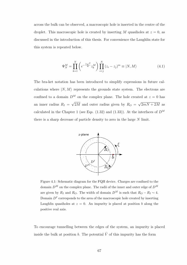
across the bulk can be observed, a macroscopic hole is inserted in the centre of the
droplet. This macroscopic hole is created by inserting M quasiholes at z = 0, as
discussed in the introduction of this thesis. For convenience the Laughlin state for
this system is repeated below.
ΨMN =
N∏k=1
(e−|zk|
2
4l zMk
) N∏i<j
(zi − zj)m ≡ |N,M〉 (4.1)
The bra-ket notation has been introduced to simplify expressions in future cal-
culations where |N,M〉 represents the grounds state system. The electrons are
confined to a domain DM on the complex plane. The hole created at z = 0 has
an inner radius RI =√
2M and outer radius given by RO =√
2mN + 2M as
calculated in the Chapter 1 (see Eqs. (1.32) and (1.33)). At the interfaces of DM
there is a sharp decrease of particle density to zero in the large N limit.
Figure 4.1: Schematic diagram for the FQH device. Charges are confined to the
domain DM on the complex plane. The radii of the inner and outer edge of DM
are given by RI and RO. The width of domain DM is such that RO −RI ∼ 4.
Domain DI corresponds to the area of the macroscopic hole created by inserting
Laughlin quasiholes at z = 0. An impurity is placed at position b along the
positive real axis.
To encourage tunnelling between the edges of the system, an impurity is placed
inside the bulk at position b. The potential V of this impurity has the form
67
V = uN∑i=1
δ(2)(zi − b). (4.2)
The parameter u corresponds to the strength of the potential which will be set to
unity and we assume that |b| = (RO +RI)/2. If the ring of the bulk is sufficiently
thick then adding the impurity to the system will have no effect on the edges
due to a finite correlation length in the bulk on the order of the magnetic length.
Therefore it is assumed that for all N the width of the system (RO−RI) is constant
and narrow enough such that both edges are affected by the impurity.
The microscopic expression for the zero mode tunnelling matrix elements due to
the impurity inserted into the bulk are given by
〈V 〉χ ≡〈N,M |V |N,M + χ〉√
〈N,M |N,M〉 〈N,M + χ|N,M + χ〉
=
∫N−1
|ΨMN |2
N−1∏i=1
zχi
N∑n=1
δ(2)(zn − b)√∫N
|ΨMN |2 ·
∫N
|ΨM+χN |2
(4.3)
where, to shorten notation inside the integrals, |ΨMN |2 is used to denote the ab-
solute value of Laughlin’s wavefunction squared and the integration variables are
shortened to∫N≡∫ ∏N
k=1 d2zk. This matrix element describes a process in which
a number χ of quasiparticles are transferred from the inner boundary to the outer
boundary due to the impurity potential V given in Eq. (4.2). Therefore χ = 1
corresponds to quasiparticle tunnelling and χ = m to electron tunnelling for some
Laughlin state ν = 1/m. Note that the denominator in (4.3) is needed to correctly
normalize the elements.
The delta-function in the numerator of Eq. (4.3) allows one of the variables in
68

the integral to be integrated out. Using the fact that the integrals appearing in
each term of the sum are symmetric with respect to the exchange of integration
variables, 〈V 〉χ can be written as
〈V 〉χ =
Ne−|b|22|b|2M bχ
∫N−1
|ΨMN−1|2
N−1∏i=1
zχi |zi − b|2m√∫N
|ΨMN |2 ·
∫N
|ΨM+χN |2
. (4.4)
The overlap integrals in Eq. (4.3) for the free fermion case can be calculated
analytically and thus provides a good check for the numerical methods developed in
this chapter. An effective numerical method to calculate these overlap integrals is
by using Monte Carlo (MC) simulations. As already discussed, this method seems
quite natural since the norm of the wavefunction can be considered as a partition
function for a 2D Coulomb plasma allowing statistical averages of operators to be
calculated with a probability distribution analogous of the Boltzmann distribution
of the plasma. All the MC simulations in the present work were carried out using
the Metropolis algorithm (see Chapter 2).
To directly use the MC method on the integral in the numerator of (4.3) is difficult
due the product over all particles of the form zχi . This product introduces a phase
problem to the calculation since the MC measurements on the phase part of this
product will have significant fluctuations between successive measurements and the
convergence of the simulation will be slow. Two successful methods to overcome
this phase problem have been found. The effectiveness of each method depends
on the value of χ and the first of the methods to be discussed is appropriate for
small values of χ whereas the second method can only be used for χ = m, i.e., for
the case of an electron tunnelling across the bulk.
69

4.1.1 Phase Problem Solution: Method 1 for χ ≤ 1
The first method of overcoming the phase problem in the integral (4.3) is by using
the cumulant expansion. It will be seen later that only for a small value of χ
can the particular cumulant expansion of interest be calculated reliably. First the
integral in the numerator should be expressed in a more convenient way. To do
this it is noted that part of the numerator of Eq. (4.4) can be re-written as;
N−1∏i=1
|zi − b|2mzχi =
(−b|b|
)χ(N−1) N−1∏i=1
|zi − b|2m|zi|χΘχ(zi, b)
where
Θχ(zi, b) =
(1− zib
) (1− b
zi
)∣∣1− zi
b
∣∣ ∣∣∣1− bzi
∣∣∣χ . (4.5)
The advantage of the function Θχ(z, b) is that its cumulant expansion can be cal-
culated with respect to some probability distribution using a MC simulation with
a relatively quick convergence. Indeed if we choose the probability distribution
such that
⟨N−1∏i=1
Θχ(zi, b)
⟩ϕ
=
∫N−1
|ΨMN−1|2
N−1∏i=1
|zi|χ |zi − b|2mΘχ(zi, b)∫N−1
|ΨMN−1|2
N−1∏i=1
|zi|χ |zi − b|2m(4.6)
then the average over Θ(z, b) in (4.6) can be related the tunnelling matrix elements
in (4.3) via
〈V 〉χ =
(−|b|b
)χ(N−1)⟨N−1∏i=1
Θχ(zi, b)
⟩ϕ
Ne|b|22 |b|2Mbχ
√h1h2, (4.7)
70

where
h1 =
∫N−1
|ΨMN−1|2
N−1∏i=1
|zi|χ|zi − b|2m∫N
|ΨMN |
, (4.8)
h2 =
∫N−1
|ΨMN−1|2
N−1∏i=1
|zi|χ|zi − b|2m∫N
|ΨM+χN |
. (4.9)
Integrals h1 and h2 are relatively trivial MC integrals to compute. Even though
the number of particles is different in the numerator and the denominator, it is
observed that the form of h1 and h2 is similar to the definition of the average of
the density operator (e.g., see Eq. (1.18)) and therefore
h1 =〈ρ〉M e
|b|22
N |b|2M
∫N−1
|ΨMN |2
N−1∏k=1
|zk − b|2m∫N−1
|ΨMN |2
N−1∏k=1
|zk − b|2m|zk|, (4.10)
h2 =〈ρ〉M+1 e
|b|22
N |b|2(M+1)
∫N−1
|ΨM+1N |2
N−1∏k=1
|zk − b|2m∫N−1
|ΨMN |2
N−1∏k=1
|zk − b|2m|zk|. (4.11)
Now the integrals in the numerator and denominator of both h1 and h2 have
the same number of integration variables and therefore the ratio of integrals can
be calculated using MC. Since it is assumed that the impurity is placed deep
within the bulk; 〈ρ(b)〉M = 〈ρ(b)〉M+1 = (2πm)−1. As already mentioned it is the
cumulant expansion of Θ(z, b) in (4.6) that gets rid of the phase problem in the
MC computations for the tunnelling matrix elements. In order to see why this is
so, consider Θ(z, b) written in terms of an exponential function.
71

eln Θ(z,b) = exp
(iχArg
[(1− z
b
)(1− b
z
)])(4.12)
The first couple of terms for the cumulant expansion of some function⟨eG⟩
is
⟨eG⟩
= e〈G〉+12!(〈G2〉−〈G〉2)+ 1
3!(2〈G〉3−3〈G〉〈G2〉+〈G3〉)+··· (4.13)
After substituting Eq. (4.12) into the expansion of Eq. (4.13) we notice the fol-
lowing; the mean field of G is essentially an average over an angle, which is zero.
Secondly, sequential terms in the expansion increase by a factor of χ. For the
cumulant expansion to be used reliably, the higher order terms must quickly decay
to zero. For χ > 1, this is not the case and the cumulent expansion converges too
slowly considering only a small, finite number of terms can be computed numeri-
cally. However for χ = 1 the cumulant expansion of 〈∏
Θ(zi, b)〉 is well behaved
and can be used to calculate the matrix elements in Eq. (4.3) reliably.
4.1.2 Phase Problem Solution: Method 2 for χ = m
The second method of avoiding the phase problem in (4.3) relies on the fact that
for the special case χ = m, then (4.3) can be written in terms of real valued
functions. The numerator of (4.3) (sticking to general χ for the moment) can be
written as follows,
〈N,M |V |N,M + χ〉 = Ne−b2
2 b2M+χ
∫N−1
|ΨMN−1|2
N−1∏i=1
zχi |zi − b|2m
72
= Ne−b2
2 b2M+χ
∫N−1
∣∣ΨMN−1
∣∣2 N−1∏i=1
|zi|2χzm−χi (zi − b)m(
1− b
zi
)m. (4.14)
The only non-zero terms of this integral are terms that conserve total angular
momentum; the remainder of the terms will be angle dependent and will go to zero
after performing the integration over the angle variables. To see what terms do
conserve angular momentum, a global transformation can be performed such that
{zi} → {zieiθ}, where θ is some constant. From performing this transformation it
can be deduced that for χ > m there are no terms in the polynomials that conserve
angular momentum and thus the tunnelling matrix elements 〈V 〉χ>m are zero for
Laughlin wave functions. Under a similar global rotation argument when χ = m,
the numerator of 〈V 〉m takes the particularly simple form
〈N,M |V |N,M +m〉 = Ne−b2/2b2M+m (−b)m(N−1)
∫N−1
∣∣ΨM+mN−1
∣∣2 . (4.15)
Therefore one can write the matrix element for the electron tunnelling as
〈V 〉m = Ne−b2
2 (−b)m(N−1)b2M+m
√Ξ2
τ. (4.16)
The integrals have all been symbolised by Ξ and τ to shorten notation and they
have the form
Ξ =
∫N−1
∣∣ΨM+mN−1
∣∣2∫N
∣∣ΨM+mN
∣∣2 , (4.17)
τ =
∫N
∣∣ΨMN
∣∣2∫N
∣∣ΨM+mN
∣∣2 . (4.18)
73

Functions Ξ and τ are simply ratios of the overlap of the ground state functions
(4.1) for various N and M values. The function τ is a relatively trivial MC
calculation, where Ξ is not so trivial due to the differing number of integration
variables in the numerator and the denominator. To form a method to compute
Ξ, consider the following average
〈F 〉N,M+m =
∫N
∣∣ΨM+mN
∣∣2 N∑i=1
f(zi)∫N
∣∣ΨM+mN
∣∣2 = N
∫N
∣∣ΨM+mN
∣∣2 f(zN)∫N
∣∣ΨM+mN
∣∣2 (4.19)
The explicit form of f(z) is chosen to be
f(zi) = Θ(|zi| − (RO + d)) =
1 for |zi| ≥ RO + d
0 otherwise,(4.20)
where d is some distance added to the outer radius and will be defined later. By
multiplying and dividing the average 〈F 〉N,M+m by∫N−1|ΨM+m
N−1 |2 then (4.19) can
be manipulated in such a way as to contain the function Ξ. I.e.,
〈F 〉N,M+m = N · Ξ ·
∫N
∣∣ΨM+mN
∣∣2 f(zN)∫N−1
∣∣ΨM+mN−1
∣∣2 = N Ξ IN . (4.21)
The remaining integrals in the expression (4.21) have been labelled by IN .
74

IN =
∫d2zNe
−|zN |2/2|zN |2(M+m)f(zN)
∫N−1
∣∣∣ΨβN−1
∣∣∣2 N−1∏i=1
|zi − zN |2m∫N−1
∣∣∣ΨβN−1
∣∣∣2= 2π
∫ ∞RO+d
drN e−r2
N/2 r2(M+m)+2m(N−1)N
⟨N−1∏i=1
∣∣∣∣1− zizN
∣∣∣∣2m⟩N−1,M+m
= 2π
∫ ∞RO+d
drN e−r2
N/2 r2(M+m)+2m(N−1)N γ(zN) (4.22)
The average over N − 1 particles is labelled as γ, which is a function of the N ’th
particle coordinate. Since it will be real valued the angle integration over the N ’th
coordinate has been performed. The function e−rN/2r2(M+m)+2m(N−1)N is a rapidly
decaying function away from the outer boundary and thus if the lower integration
limit of rN is sufficiently larger than RO, then one can use the following asymptotic
approximation γ(zN) ∼ γ(RO+d). This substitution makes the function γ(RO+d)
trivial to calculate using a MC simulation. Once γ(RO + d) is known, the integral
IN is a straightforward two-dimensional integral.
Alongside the γ-function, the average 〈F 〉 must also be calculated using an MC
simulation. This average is also dependent on d, the distance from the outer
boundary. Since 〈F 〉 simply counts the number of particles beyond the point
RO + d there is a trade-off as to how large d should be. The larger the value of
d the fewer particles there will be to count since the particle density decreases
sharply from the outer boundary, but also for larger values of d, the more accurate
the asymptotic approximation, γ(zN) ∼ γ(RO +d), thus a trade off must be made.
With Ξ now define in terms of computable MC integrals,
Ξ =〈F 〉N,M+m
NIN, (4.23)
then the zero mode tunnelling matrix elements satisfying χ = m can be expressed
75

in terms of these MC integrals as follows,
〈V 〉m = e−|b|2/2(−b)m(N−1)b2M+m
〈F 〉N,M+m
IN√τ
. (4.24)
Therefore the zero mode tunnelling matrix elements due to an impurity in the bulk
can be computed for the two special cases; χ = m given in terms of MC averages
in (4.24) and, for χ = 1 which has also been expressed in terms of MC averages in
the previous part of this section (4.7). In the next section, analogous expressions
for the tunnelling matrix elements will be formulated in the effective theory.
4.2 Zero Mode Tunnelling Matrix Elements Us-
ing the Effective Hamiltonian
As implied in the introduction, it is the edges of the device, consisting of two
counter propagating chiral Luttinger liquids that are of most interest for tunnelling
calculations. A successful method for describing the effective low-energy physics of
a chiral Luttinger liquid uses the method of bosonisation which has been discussed
in Chapter 3 where the bosonised fields for quasiparticle operators were derived.
For convenience they are stated below.
ψ†p,O(ξ) = eipmϕN epφO(ξ)
ψp,O(ξ) = e−pφO(ξ)e−ipmϕN
ψ†p,I(ξ) = eipmϕN eipϕM epφI(ξ)
ψp,I(ξ) = e−pφI(ξ)e−ipmϕN e−ipϕM (4.25)
76

The subscript “I” corresponds to an inner boundary operator and “O” to an outer
boundary operator. The fields φO/I are bosonic and are given by
φO(ξ) = −iξR
(θN +θMm
) +∑k>0
√1
mk
(e−ik
ξRa†k − e
ik ξRak
)= φ0
O + φ+O − φ
−O
φI(ξ) = − iξ
mRθM +
∑k>0
√1
mk
(eik
ξRa†−k − e
−ik ξRa−k
)= φ0
I + φ+I − φ
−I . (4.26)
In the effective theory of low-energy excitations the transverse positions to the
edges of the FQH device are unimportant since we assume that the domain DM is
a very narrow ring in comparison to the size of its outer radius RO, therefore our
particle fields depend only on the longitudinal coordinate ξ, where ξ ∈ [0, 2πR]
and R is the radius at which the transfer of charges between the edges takes place.
I.e., R ≡ |b|. In (4.25), ψp corresponds to the annihilation operator of particle with
charge e∗ = (p/m)e in the Laughlin state ν = (1/m). Therefore ψp=1 corresponds
to the field for a single Laughlin quasiparticle with charge e∗ = (1/m)e and ψp=m
corresponds to m quasiparticles, or equivalently a single electron field.
With the low-energy, effective theory field operators defined, one can now discuss
the effect of the impurity placed in the bulk. The tunnelling operator takes the
form
HT =∞∑p=1
Ap(ξ), (4.27)
where ξ is the longitudinal position at which tunnelling occurs along the boundaries
and the operators Ap transfer a number of p quasiparticles from the inner to the
outer boundary. From the form of HT one can see it is possible for the tunnelling
77

of any number of quasiparticles across the bulk. For p = 1, AP describes the
tunnelling process for a single quasiparticle and for p = m the tunnelling process is
for that of an electron in FQH state ν = 1/m. For Laughlin states, however, it was
shown (see Eq. (4.14)) that the transfer of p > m quasiparticles is identically zero.
Whether this behaviour should be extended to the exact wave functions of quantum
Hall states is unknown and, thus experiments on FQH systems that observe a
p > m tunnelling process would be extremely interesting and a good measure for
the preciseness of the Laughlin wavefunction as a microscopic description of the
FQHE.
Here two types of tunnelling processes across the bulk are considered, the first
being a single quasiparticle tunnelling and the second will be electron tunnelling
or equivalently m quasiparticles tunnelling. These processes are described by Ap=1
and Ap=m respectively. In general operators Ap have the form;
Ap(ξ) = tp
(ψ†p,O(ξ)ψp,I(ξ) + h.c.
), (4.28)
where ξ is the longitudinal position at which the tunnelling occurs on the bound-
aries and tp is a parameter that cannot be calculated analytically given the mi-
croscopic theory. In this work the scaling behaviour of the parameters tp will be
investigated as system size N is varied. This can be achieved by looking at the
zero mode matrix elements of the tunnelling operator.
〈Ap(ξ)〉 = 〈N,M |Ap(ξ) |N ′,M ′〉
= tp 〈N,M |ψ†p,O(ξ)ψp,I(ξ) |N ′,M ′〉+ h.c. (4.29)
= tp 〈N,M | eipmϕN epφO(ξ)e−pφI(ξ)e−i
pmϕN e−ipϕM |N ′,M ′〉+ h.c.
The first term in (4.29) describes a process where p particles move from the inner
boundary to the outer boundary and for the second term this process is reversed.
78

Only one term is needed here so the Hermitian conjugate term can be neglected.
Next the ordering of the operators is considered which will in turn affect the
behaviour of the parameter tp. Here, two types of ordering are considered with
the first being the usual definition of normal ordering defined by
eφ →: eφ : = eφ0
eφ+
e−φ−. (4.30)
The matrix element calculated using this ordering is denoted by 〈: Ap(ξ) :〉 and is
straightforward to calculate.
|〈: Ap(ξ) :〉| =∣∣∣⟨N,M ∣∣∣ei pmϕN : epφO(ξ)e−pφI(ξ) : e−i
pmϕN e−ipϕM
∣∣∣N ′,M ′⟩∣∣∣
= |tp|δN,N ′δM,M ′−p (4.31)
The absolute values of matrix elements are taken to get rid of unnecessary phase
terms. Therefore if normal ordering is used, only tp contributes to system size
dependence. On the other hand, a different result is obtained by choosing the
following ordering for the operators,
eφ = eφ0
eφ+
e−φ−e−
12
[φ0,φ+−φ−]e−12
[φ+,−φ−] = eφ0
eφ+
e−φ−e−
12
∑k(m
k), (4.32)
where the following commutation relations have been used; [φ0x(ξ), φ
+x (ξ)−φ−x (ξ)] =
0 and [φ+x (ξ), φ−x (ξ)] = −
∑k(m/k) where x = I or, x = O. These relations are
straightforward to calculate using the commutators listed in Chapter 3 for the zero
mode operators and a±k, a†±k. Proceeding with the matrix element (4.29),
79
|〈Ap(ξ)〉| = |tp| exp
(−∑k>0
p2
mk
)δN,N ′δM,M ′−p (4.33)
The sum over k in (4.33) has already been calculated in Chapter 3, see Eq.
(3.31). It was calculated using a soft cutoff Λ ∼ R ≡ |b| to give∑
k>0 k−1 →∑
k>0 k−1e−k/R = − ln(1 − e−1/R). To get an approximate idea of the behaviour
of this sum in the large N , or equivalently large R limit, the exponential in the
logarithm can be expanded to give − ln(1− e−1/R) ∼ lnR. Thus for a log-log plot
of the amplitude of (4.33) versus particle number, one would expect the gradient
to be ∼ −p2/m for large enough R ≡ |b|. For now we will keep the exact form of
the sum so that the final expression of the tunnelling matrix elements is,
|〈Ap(ξ)〉| = |tp|(
1− e−1R
) p2mδN,N ′δM,M ′−p. (4.34)
From (4.34); the zero mode tunnelling matrix elements have a dependence on
the system size N , which for non-normal ordering of operators given by (4.32) is
not from the parameter tp. If the operator Ap for ordering (4.32) is local then
we can assume all the system size dependence originates from the sum∑
k k−1
and tp is constant for all N . Ideally the tunnelling operators should remain local
since the impurity placed between the edges in the FQH device should only affect
charges in its vicinity and not the remainder of the system. The correlator of
a local operator 〈Ap(ξ)Ap(ξ′)〉 should be independent of system size for ξ and ξ′
sufficiently far apart, also ξ, ξ′ should be sufficiently far away from the edges of
the system.
〈Ap(ξ)Ap(ξ′)〉 = 〈N,M |Ap(ξ)Ap(ξ′) |N ′,M ′〉
= 2 exp
{2p2
m
∑k>0
k−1
(cos
[k
R(ξ′ − ξ)
]− 1
)}× cos
[ pR
(N − p
m
)(ξ′ − ξ)
](4.35)
80

Only matrix elements that are kept in the above expression are those with M ′ = M
and N ′ = N which satisfies the definition of the tunnelling operator Ap.
To finish the calculation, a soft cutoff is used (Λ ≡ R) to calculate the sum in (4.35),
which is the same approach as was used to calculate similar sums earlier for the
tunnelling matrix elements. Using this cutoff and taking the limit |ξ− ξ′|/R << 1
gives the final result for the correlator calculation in Eq. (4.36). There is no system
size independence as required for the correlator of the tunnelling operator using
the operator ordering defined in Eq. (4.32).
〈Ap(ξ)Ap(ξ′)〉 =2
(1 + (ξ′ − ξ)2)p2
m
cos[ pR
(N − p
m
)(ξ′ − ξ)
](4.36)
The correlator of the tunnelling operator for normal ordering, 〈: Ap(ξ) :: Ap(ξ′) :〉
does have system size dependence and therefore tunnelling operators Ap defined
by ordering (4.32) are preferred. To summarise this section; expressions for the
zero mode matrix tunnelling elements have been calculated for both normal or-
dered operators (4.31) and for non-normal ordered operators (4.34). In the normal
ordered case there is system size dependence which must be encoded in the pa-
rameter tp. For the non-normal ordered tunnelling operators, this size dependence
comes from the calculation of the matrix elements and the operator algebra itself.
Since the non-normal ordered tunnelling matrix elements show explicit size depen-
dence and were obtained from local tunnelling operators, it is expected that these
results should manifest from the microscopic theory also. Therefore we would ex-
pect to see the same system size dependence from 〈Ap(ξ)〉 and the microscopic
matrix elements 〈V 〉p. In the next section the details, and the results of the MC
computations will be discussed.
81

4.3 Results for Zero Mode Tunnelling Matrix El-
ements
After showing the formulation for the microscopic computations, the results of the
simulations can now be discussed. They are shown in the later parts of this section.
To begin, details for the particular states and system sizes of MC simulations are
presented.
4.3.1 Simulation Details
To run the MC simulations for the zero mode tunnelling matrix elements, the
filling factors chosen for the computations were ν = m−1 = 1/3 and ν = m−1 = 1.
The free fermion case provides a good check for the numeric methods used since
for this state, all matrix elements of form (4.3) can be calculated analytically. See
the Appendix A for a more detailed discussion.
When considering tunnelling across the bulk in a FQH device, there are two partic-
ularly interesting cases. According to the literature discussed in the introduction
to this thesis, for Laughlin states the most favourable form of tunnelling is for a
single quasiparticle (χ = 1). The other interesting case is for when an electron
tunnels across the bulk. In most other systems, as well as in the FQH system in
the strong back scattering regime, charge is usually transported by electrons. For
these reasons, MC simulations have been run for χ = 1 and χ = 3.
Equations (4.7) and (4.24) give the forms for the tunnelling operators in terms of
MC integrals for the tunnelling of a single quasiparticle and three quasiparticles
respectively. It is noted that in the free fermion case where ν = 1, electrons are
transported across the bulk rather than Laughlin quasiparticles and for χ > 1,
all the matrix elements in Eq. (4.3) are zero. Therefore both methods presented
82

in the previous two sections to overcome the phase problem are equivalent to one
another in the free fermion case ν−1 = χ = 1. The results listed for the free
fermion case in the next section were obtained using method 1.
For the less trivial state ν = 1/3, MC calculations according to method 1 were used
to calculate the zero mode tunnelling matrix elements for a single quasiparticle and
method 2 was used for three quasiparticles/one electron tunnelling. In method 1,
for both ν = 1 and ν = 1/3 the cumulant expansion (4.13) was computed up to
the tenth cumulant. For method 2; there is an additional value d that appears in
the integrals (4.19) and (4.22), which was defined as some length away from the
outer boundary. An appropriate value (found via a numerical calculation in the
free fermion state) to minimise systematic errors was found to be d = 3 magnetic
lengths.
It is the system size dependence of the matrix elements given by (4.3) that is
of interest and so multiple simulations where performed for various values of N
ranging from 20 to 200 electrons. For all values of N , the width of the system
between the two edges was always kept constant such that RO − RI ∼ 4 units of
magnetic length. This was achieved by varying the value of M accordingly with
the number of electrons, N . The only important statement about the placement
of the impurity is that it was equal distance from the inner and outer edge, i.e.,
|b| = (RO + RI)/2. Changing the argument of b has no physical effect on the
tunnelling due to the axial symmetry of the system. For simplicity these results
were obtained by choosing b to be along the positive real axis.
4.3.2 Tunnelling Results for ν = 1
The zero mode tunnelling matrix elements in the free fermion case were calculated
microscopically according to (4.7) where the averages were computed using MC.
The only non zero matrix element (excluding the trivial χ = 0 case) is when a
83

single electron is being transferred across the bulk corresponding to χ = 1 in (4.7).
These results are presented graphically on a log-log plot in Figure 4.2.
Figure 4.2: Curve for the logarithm of the zero mode quasiparticle tunnelling
operator versus the logarithm of N as calculated using Monte Carlo for filling
factor ν = m−1 = 1. The points are the data from the Monte Carlo calculations,
whilst the linear curve is the line of best fit as shown in Eq. (4.37).
The data set plotted on Figure 4.2 is fitted to straight a line where the gradient
of the line for ν = 1 is given by,
d ln 〈V 〉1d lnN
= −0.972± 0.006 (for ν = 1) (4.37)
The tunnelling matrix elements obviously have a system size dependence. There-
fore when comparing these numerical results to the effective theory results for the
tunnelling operator, operator ordering defined in (4.32) must be imposed for a
constant tp.
In the simulations, the impurity was placed at position b along the real axis and
84
so in the effective theory calculation ξ = 0 and R = |b|. These parameters allow
us to drop the absolute value of the matrix elements since the phase terms drop
out anyway. Setting p = χ = 1 in (4.34) gives
d ln 〈A1〉d lnN
= −0.966 (for ν = 1). (4.38)
Comparing (4.38) to (4.37) shows that the effective theory, when using non-normal
ordered operators does match the microscopic computations for the zero mode
tunnelling matrix elements.
4.3.3 Tunnelling Results for ν = 1/3
For the filling factor ν = 1/3 tunnelling matrix elements were computed for both a
quasiparticle (χ = 1) and an electron (χ = 3) tunnelling across the bulk. Method
1 (4.7) was used for the quasiparticle tunnelling case and method 2 (4.24) for elec-
tron tunnelling. The data from both MC simulations is presented on a log-log plot
in Figure 4.3.
The gradient of linear curve fitted to the χ = 1 data set is;
d ln 〈V 〉1d lnN
= −0.308± 0.003 (for ν = 1/3). (4.39)
Following similar arguments to those given in the results section for ν = 1; the
effective theory prediction for the tunnelling matrix elements for a quasiparticle
transferred across the bulk is
d ln 〈A1〉d lnN
= −0.331 (for ν = 1/3). (4.40)
85

Figure 4.3: Curve for the logarithm of the zero mode tunnelling matrix elements
versus the logarithm of N as calculated using MC for filling factor ν = m−1 =
1/3. The points are the data collected from the MC computations for χ = 1
and χ = 3, whilst the curves are lines of best fit shown in equations (4.39) and
(4.41) corresponding to a quasiparticle and electron respectively.
Comparing (4.40) to (4.39); the effective theory does not predict the correct scal-
ing behaviour for the zero mode tunnelling matrix elements from the tunnelling
Hamiltonian.
This author doubts that the difference between the effective theory and the nu-
merical calculation for a single quasiparticle tunnelling in the ν = 1/3 state is a
consequence of the numerical method used. Recall, for χ = 1, method 1 was used
within the MC calculation to compute the tunnelling matrix element, which makes
use of the cumulent expansion. Therefore there is a possibility that systematic er-
rors have appeared as a consequence of computing only a finite number of terms
for the cumulent expansion. This argument, however does not seem plausible for
the following reason; this cumulent expansion method was also used to compute
electron tunnelling in the free fermion case, where the results matched those of the
effective theory predictions. Since higher-order terms in the cumulent expansion
86
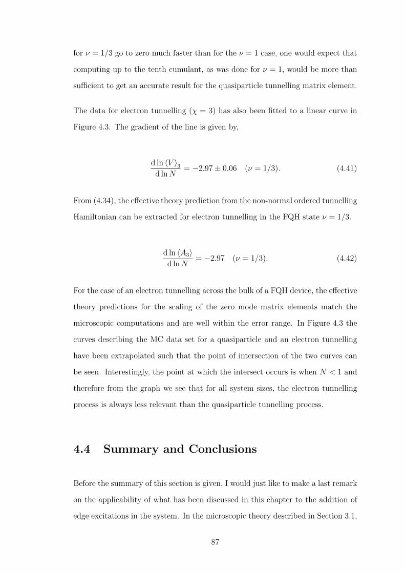
for ν = 1/3 go to zero much faster than for the ν = 1 case, one would expect that
computing up to the tenth cumulant, as was done for ν = 1, would be more than
sufficient to get an accurate result for the quasiparticle tunnelling matrix element.
The data for electron tunnelling (χ = 3) has also been fitted to a linear curve in
Figure 4.3. The gradient of the line is given by,
d ln 〈V 〉3d lnN
= −2.97± 0.06 (ν = 1/3). (4.41)
From (4.34), the effective theory prediction from the non-normal ordered tunnelling
Hamiltonian can be extracted for electron tunnelling in the FQH state ν = 1/3.
d ln 〈A3〉d lnN
= −2.97 (ν = 1/3). (4.42)
For the case of an electron tunnelling across the bulk of a FQH device, the effective
theory predictions for the scaling of the zero mode matrix elements match the
microscopic computations and are well within the error range. In Figure 4.3 the
curves describing the MC data set for a quasiparticle and an electron tunnelling
have been extrapolated such that the point of intersection of the two curves can
be seen. Interestingly, the point at which the intersect occurs is when N < 1 and
therefore from the graph we see that for all system sizes, the electron tunnelling
process is always less relevant than the quasiparticle tunnelling process.
4.4 Summary and Conclusions
Before the summary of this section is given, I would just like to make a last remark
on the applicability of what has been discussed in this chapter to the addition of
edge excitations in the system. In the microscopic theory described in Section 3.1,
87

edge excitations {n±k}, where n±k are the occupation numbers of the k’th orbital
on the inner “-” or outer “+” boundary are described by Laughlin’s wavefunction
multiplied by a series of power sum polynomials Sn±k±k .
|{n±k}, N,M〉 =∏k>0
Sn±k±k ΨM
N (4.43)
Similarly in terms of the chiral Luttinger liquid formalism, the same set of occupied
orbitals can be obtained by applying the boson creation operator a†±k to the ground
state.
|{n±k}〉 =∏k>0
a†±k |N,M〉 (4.44)
Therefore a similar procedure to the one described in this chapter can also be
used to numerically check the effective Hamiltonian for more complicated states
where not only has charge been transferred between edges, but also the occupation
configuration of excited orbitals has also been altered. If the effective Hamiltonian
does match the microscopic model then it is expected
⟨{n′±k}
∣∣V |{n±k}〉M→M+χ ≡
⟨N ′,M ′
∣∣∣∣∣∏p>0
a±pAχ(ξ)∏k>0
a†±k
∣∣∣∣∣N,M⟩, (4.45)
where V is the potential of the impurity inserted into the bulk and Aχ(ξ) is the
effective tunnelling operator in Eq. (4.28).
This work has investigated the zero mode tunnelling matrix elements due to an
impurity in the bulk, which have been computed as a function of system size, N
and then compared to the effective theory predictions for the effective tunnelling
operators. In Section 4.2, the effective theory predictions were discussed. The
88
quasiparticle operators from the Luttinger liquid theory of FQH edge states were
used to calculate the zero mode matrix elements of the tunnelling operators Ap,
where p corresponded to the number of quasiparticles tunnelling at the impurity.
These matrix elements were calculated using two types of ordering of quasiparticle
operators. The first type was the usual definition of normal ordering defined
in Eq. (4.30), where it was found that only the tunnelling parameter tp could
contain system size dependence. The second type of ordering considered was when
the operators were not normal ordered, as defined in Eq. (4.32). These matrix
elements did show signs of system size dependence. To investigate which scaling of
the tunnelling parameters tp best describes the tunnelling events in a FQH system,
a microscopic calculation was performed.
This microscopic calculation was based on the Laughlin states of the FQHE and
was the subject of Section 4.1. The microscopic formula that describes the process
for the tunnelling of χ particles due to the impurity inserted in to the bulk is given
by 〈V 〉χ in (4.3). The only known way of calculating such integrals in (4.3) was
by using numerical methods. The MC method was chosen for the computation of
〈V 〉χ, though to directly calculate this average would not be very efficient due to a
phase problem encountered in the simulation. This phase problem manifest itself
by causing a slow convergence of the simulation whilst computing the tunnelling
matrix elements.
Two methods were found to overcome this problem. Method 1. used MC to
calculate the cumulant expansion of a function related to 〈V 〉χ and was suitable
only for χ ≤ 1. Method 2. to overcome the phase problem was applicable only for
χ = ν−1, in which case the matrix elements in 〈V 〉χ could be written in terms of
real valued functions, thus avoiding any phase problems.
Finally, the results of the MC calculations for 〈V 〉χ were presented and compared to
the effective theory predictions of the tunnelling behaviour. It was found that the
electron tunnelling Hamiltonian predicted by the effective theory is an accurate
89

representation of the effects on the zero modes of the edges when an impurity
is inserted into the bulk of a ν = 1/3 Laughlin state. The predictions from
quasiparticle tunnelling Hamiltonian however, were significantly different to the
microscopically computed result. Emphasised in Section 4.3.3, there is no obvious
cause of an error arising from the microscopic computation.
For future work, I think there are two possible avenues of investigation to look
more closely at possible discrepancies of the effective theory for the tunnelling
matrix elements in the Laughlin states. The most obvious one would be to test
quasiparticle tunnelling for other Laughlin filling fractions, such as ν = 1/5. Initial
tests for such a calculation were conducted (using method 1, i.e. cumulant expan-
sion method) and it was found that numerically, this would be a time consuming
computation since the size of the cumulants are so small, many measurements
would need to be taken for an accurate result for the matrix elements. The second
potentially interesting avenue of investigation would be to investigate two quasi-
particles tunnelling at the impurity and see how the results would match up to
the predictions from the effective theory tunnelling operator. Again, to calculate
these matrix elements numerically would be time consuming compared to the cal-
culations computed so far in this chapter, namely because method 1 and method
2, introduced in Sections 4.1.1 and 4.1.2, could not be applied to the case when
two quasiparticle tunnel across the FQH bulk states.
There can be some agreement found between the microscopic computations and the
effective theory, shown in Figure 4.3 for filling fraction ν = 1/3. When increasing
the system sizes of the FQH device the electron operator plays a less important
role than that of the quasiparticle operator. This can be seen for all system sizes
and supports previous works mentioned in the introduction when the the electron
tunnelling term is dropped in comparison to the quasiparticle tunnelling process.
It is unfortunate that the behaviour of the most predominant tunnelling channel
(i.e. that of the quasiparticle) is the one in which there is a possibility of a
90

discrepancy in effective theory. Such computations involving tunnelling at an
impurity are an important link to experiments which use point contacts to measure
quasiparticle charge and the type of statistics they obey. In particular, shot noise
experiments involving measurements on the back scattered current (and therefore
will be dependent on the tunnelling matrix elements at the point contact) should
shed some light onto the correct scaling behaviour of the the tunnelling matrix
elements with system size. These experimental measurements would also need to
be accurate enough to distinguish between the numbers of magnitudes given in
(4.40) and (4.39).
The final conclusion for this section is that there is a possible discrepancy between
the tunnelling matrix elements calculated microscopically and the tunnelling ma-
trix elements predicted for the effective quasiparticle tunnelling Hamiltonian in
the Laughlin state ν = 1/3. It is unlikely that this discrepancy is a consequence of
the cumulant expansion method used to obtain the microscopic theory and thus
it is concluded there is possibly an error arising from the effective theory itself.
There has previously been some experimental work measuring quasiparticle charge
where the result did not agree with the predictions from the effective theory. This
supports the claim that the effective tunnelling Hamiltonian may not be a com-
plete theory in describing the tunnelling of quasiparticles between two edges in the
FQHE. A discussion of these works were given in Section 1.5 of the introduction
to this thesis. The effective theory however, for an electron tunnelling across the
bulk of a FQH device was shown to be in good agreement with the microscopic
computations of the tunnelling matrix elements.
91

Chapter 5
Numerical Testing for the Free
Energy Expansion in the
Semi-classical Limit
In the previous chapter, it is was shown that at a quantum point contact (QPC)
in the FQHE, there is a possible error with the formulation of the effective theory
Hamiltonian describing the tunnelling process of a Laughlin quasiparticle. There is
also some experimental evidence suggesting that tunnelling processes in Laughlin
states may not be accurately described by the effective tunnelling Hamiltonian [60].
This cited work was based on a shot noise experiment, involving measurements on
the back scattered current at a QPC. It was proposed that some differences between
the predictions of the effective theory and the experimental measurements could
be a consequence of the electrostatic reconstruction caused by the gates creating
the QPC. Therefore it is natural to want a description of the effects an external
electric field has on the surrounding charge density of the point contact. However,
in literature, the description of how the equilibrium density of the electrons in the
QH fluid behaves as a result of an applied external field is open to debate.
In fact there has been two differential equations derived, using completely different
92

methods, and each gives different functions of the equilibrium QH charge density
as a function of the external field. Therefore, to further shed light on the nature
of electrostatic reconstruction at a QPC in the future, one must first determine
which one of the two expressions for the charge density is accurate.
These differential equations for the equilibrium charge density in a QH droplet
will be referred to as Liouville-type equations, since their forms are similar to a
Liouville differential equation, the only difference being a non-zero term on the
right-hand-side. The first Liouville-type equation to be introduced was derived by
Zabrodin et al. in the semi-classical limit using Ward identities, the formula taken
from the work [97] is quoted below.
−~(2−m)
8π∆ ln ρ0(z) +mρ0(z) = σ(z), (5.1)
where m is the inverse filling factor of the quantum Hall state, ~ is a function
of magnetic length, the explicit relation will be given later, and σ(z) is related
to the background charge density due to the external potential. The notations
used in the works by Zabrodin et al. are explained in detail in the next section
of this chapter. A similar Liouville equation has been derived by Cheianov et al.
[98]. This calculation was carried out by reformulating Laughlin-type systems to
a boson field theory using the grand partition function. The method is discussed
in Appendix B where this Liouville-type equation is given in (B.17); it is restated
below to make a comparison with (5.1),
1
4π∆ ln ρ0(z) +mρ0(z) = mρbg(z). (5.2)
The terms on the right of Eqs. (5.2) and (5.1) are equivalent since in Zabrodin
et al.’s notation, σ(z) = mρbg(z). There is however a difference in the coefficient
of the terms containing the Laplacian. Eq. (5.1) appears to have an extra term
93

proportional to m∆ ln ρ0 that does not appear in (5.2).
To attempt to resolve the issue of which Liouville-type equation is most accurate,
Zabrodin et al.’s equation will be tested indirectly by a microscopic calculation
using the MC technique. This indirect test can be done by noting that in the
literature by Zabrodin et al. [97, 99–101], they use the plasma analogy to define
an effective free energy for the QH system. The authors then derive the free energy
expansion in the large N limit, and the method in which they use to do this, is
the same as the method used to derive the Liouville-type equation in (5.1). Thus
testing the free energy expansion will give some insight into the accuracy of the
different methods used to derive both (5.1) and (5.2).
The next section contains a brief introduction to the work carried out by Zabrodin
et al. [97, 99–101]. In Section 5.2 the analytic form of the Free energy expansion
is calculated; Sections 5.3 and 5.4 discuss how the Free energy expansion can be
computed numerically using MC. The results for this work are presented in Section
5.5 and the chapter ends with a summary and conclusion given in Section 5.6.
5.1 Introduction to the Formalism Used in the
Free Energy Expansion
The notations that are used in the work by Zabrodin et al. are quite different
to the notations used in the previous chapters and thus this chapter starts with
an introduction to the formalism used to obtain the free energy expansion of a
quantum fluid with the same interactions as described in the plasma analogy of
the Laughlin states. Note that here the geometry considered is a simple droplet
with a single boundary; there are no quasiholes inserted into the system. Using
Laughlin’s plasma analogy, the norm of Laughlin’s wavefunction can be considered
effectively as a partition function of the form
94

ZN =
∫ N∏k=1
(d2zk e
W (zk)/~) N∏i<j
|zi − zj|2m, (5.3)
where ~ = 2l2B. When the external potential W (z) takes the form W (z) = −zz,
the partition function is related to the absolute ground state of Laughlin’s wave-
function. Following the cited work [97, 99–101], we assume that the radius of the
quantum fluid is kept constant for any value of N . This is only possible if the
magnetic length, lB becomes a function of particle number N . Recall that Laugh-
lin’s wavefunction describes a circular quantum fluid with radius R = lB√
2mN
and so, for this radius to be kept constant, lB = R/(√
2mN). In accordance with
the cited work, rather than referring to the magnetic length we use the variable
~ = R2/(mN). An important result obtained by Zabrodin et al. is that in the
large-N limit (or equivalently in the limit ~ → 0) the effective free energy of the
2D Coulomb plasma has the expansion
F
~2= lnZN = c(N) +
F0
~2+F 1
2
~+O(~0). (5.4)
It is emphasised that the limit is taken in such a way that ~ → 0, N → ∞
whilst N~ is kept constant. Before writing the expression for each of the terms in
the expansion we first introduce some terminology used in the description of the
system. To take into account the obvious increase in density as N increases, the
particle density is now defined as
ρ(z) = ~N∑i=1
δ(2)(z − zi). (5.5)
Therefore the constant value in the large-N expansion is defined by
95

N~ =
∫d2zρ(z). (5.6)
The 2D Coulomb potential of the plasma is
Φ(z) = −~∑i=1
ln |zi − z|2m
= −m∫
d2ζ ln |z − ζ|2ρ(ζ), (5.7)
where the transformation to an integral in the second line holds in the large N
limit considered here and the density is defined in the following manner,
ρ(z) = − 1
4πm∆Φ(z) = ~
N∑i=1
δ2(z − zi). (5.8)
When the charges are in their equilibrium position, denoted by 〈ρ(z)〉 ≡ ρ0(z), the
2D Coulomb plasma potential is denoted as
Φ0(z) = −m∫
d2ζ ln |z − ζ|2ρ0(ζ). (5.9)
The condition for the equilibrium charge distribution is such that the energy ε is
maximised. The energy can be extracted from the partition function (5.3) using
ZN =∫Ne−~
−1ε.
− ε~
= m
N∑i 6=j
ln |zi − zj|+1
~
N∑i=1
W (zi), (5.10)
where it is a double sum in the first term following from∑
i<j ln |zi − zj| =
96

(1/2)∑
i 6=j ln |zi − zj|. By taking the continuum limit for the energy in (5.10),
which holds for scales much larger than the average spacing between particles, a
general expression for the free energy can be obtained,
F = ~2 lnZN = m
∫d2zd2z′ρ(z)ρ(z′) ln |z − z′|+
∫d2zρ(z)W (z). (5.11)
The first term in the free energy expansion, F0 in (5.4), is given by (5.11) when
the density corresponds to the equilibrium density of charges ρ0(z).
F0 = ~2 lnZN = m
∫d2zd2z′ρ0(z)ρ0(z′) ln |z − z′|+
∫d2zρ0(z)W (z) (5.12)
A convenient method to find ρ0 is to note that when the system of charges is in
an equilibrium distribution, the energy ε is maximised. The maximum energy is
given by
∂ε
∂zi= −m~
∑j=16=i
1
zi − zj− ∂W (zi)
∂zi= 0 (5.13)
Therefore when this condition holds, the density is given by ρ0. Taking the ex-
pression (5.13) to the continuum limit we have
∂
∂z(Φ0(z)−W (z)) = 0, (5.14)
where Φ0(z) is given by (5.9). Differentiating (5.14) with respect to z allows
the equilibrium density to be expressed in terms of the Laplacian of the external
potential which provides a trivial calculation for ρ0:
97
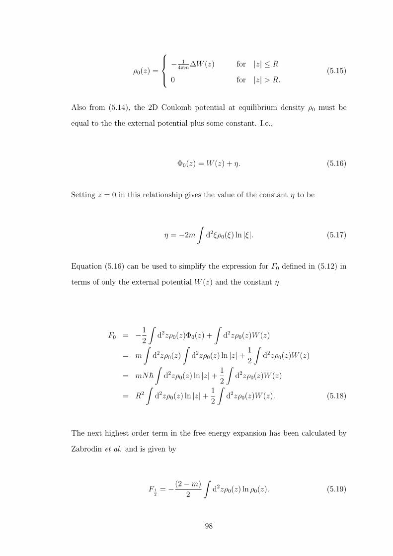
ρ0(z) =
−1
4πm∆W (z) for |z| ≤ R
0 for |z| > R.(5.15)
Also from (5.14), the 2D Coulomb potential at equilibrium density ρ0 must be
equal to the the external potential plus some constant. I.e.,
Φ0(z) = W (z) + η. (5.16)
Setting z = 0 in this relationship gives the value of the constant η to be
η = −2m
∫d2ξρ0(ξ) ln |ξ|. (5.17)
Equation (5.16) can be used to simplify the expression for F0 defined in (5.12) in
terms of only the external potential W (z) and the constant η.
F0 = −1
2
∫d2zρ0(z)Φ0(z) +
∫d2zρ0(z)W (z)
= m
∫d2zρ0(z)
∫d2zρ0(z) ln |z|+ 1
2
∫d2zρ0(z)W (z)
= mN~∫
d2zρ0(z) ln |z|+ 1
2
∫d2zρ0(z)W (z)
= R2
∫d2zρ0(z) ln |z|+ 1
2
∫d2zρ0(z)W (z). (5.18)
The next highest order term in the free energy expansion has been calculated by
Zabrodin et al. and is given by
F 12
= −(2−m)
2
∫d2zρ0(z) ln ρ0(z). (5.19)
98

Higher orders of the expansion have been calculated in the cited works [97, 99–
101], though these are not taken into account for the computations carried out in
this Thesis. The aim of the remainder of this chapter is to test via a numerical
computation if the free energy expansion in the large-N limit does display the
behaviour described, in particular by the term F 12. The numerical method used
in this work is Monte Carlo and it is convenient for this method to calculate
the difference of the free energy expansions for two similar systems rather than
calculating the free energy expansion directly. To do this we consider three different
potentials, W0, W1 and W2 for which the free energy expansion can be calculated
analytically using the model by Zabrodin et al. This is discussed in Section 5.2.
These free energy expansions can then be compared to numeric computations of
the differences in the free energy expansions of W1 with W0 and also W2 with W0,
which is described in Section 5.3 in more detail.
5.2 Analytic Expressions for the Free Energy Ex-
pansions for Particular Choices of W (z)
In this section the free energy expansions in the large N limit are calculated for
particular choices of potential W (z) according to the model by Zabrodin et al. The
first choice of external potential, W0(z) is chosen such that the partition function
(5.3) is equivalent to the magnitude squared of the Laughlin wavefunction. For this
system, the equilibrium particle density is simply a constant ρ(0)0 inside the domain
confining the charges. Since this is the simplest choice of external potential, this
system will be discussed first in Subsection 5.2.1. External potentials W1 and W2
will correspond to systems where the density of charges has been slightly deformed
from the constant value ρ(0)0 . In particular, the later two external potentials have
been chosen to reproduce relatively straight forward expressions to be computed
numerically.
99
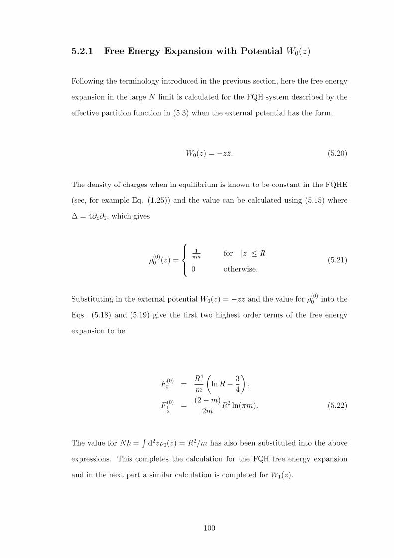
5.2.1 Free Energy Expansion with Potential W0(z)
Following the terminology introduced in the previous section, here the free energy
expansion in the large N limit is calculated for the FQH system described by the
effective partition function in (5.3) when the external potential has the form,
W0(z) = −zz. (5.20)
The density of charges when in equilibrium is known to be constant in the FQHE
(see, for example Eq. (1.25)) and the value can be calculated using (5.15) where
∆ = 4∂z∂z, which gives
ρ(0)0 (z) =
1πm
for |z| ≤ R
0 otherwise.(5.21)
Substituting in the external potential W0(z) = −zz and the value for ρ(0)0 into the
Eqs. (5.18) and (5.19) give the first two highest order terms of the free energy
expansion to be
F(0)0 =
R4
m
(lnR− 3
4
),
F(0)12
=(2−m)
2mR2 ln(πm). (5.22)
The value for N~ =∫
d2zρ0(z) = R2/m has also been substituted into the above
expressions. This completes the calculation for the FQH free energy expansion
and in the next part a similar calculation is completed for W1(z).
100

5.2.2 Free Energy Expansion with Potential W1(z)
For the FQH system, the equilibrium density was constant inside the domain
confining the charges. Since it is convenient to calculate the difference of the
free energy expansions within the confines of the numerical method used, here we
will discuss the free energy expansion for a slightly more complicated equilibrium
density profile which will in turn affect the form of the external potential W1(z).
The density profile considered here is one which is still radially symmetric, however
it has a maximum value at z = 0 and decreases linearly to the radius of the droplet
of charges:
ρ(1)0 (z) =
κ+ (ρ
(0)0 − κ)
|z|R1
for |z| ≤ R1
0 otherwise,
(5.23)
where ρ(0)0 = 1/(πm) is the value of the equilibrium distribution of charges for
potential W0(z) as discussed in the previous subsection and κ is a constant with
a value slightly increased from ρ(0)0 . A sketch of this density profile is shown in
Figure 5.1.
The difference in free energy between the system with the density as described in
(5.23) and the FQH system is taken for a given value of particle number N . Since
the density will be overall larger for this system than the FQH system, this implies
that if we wish for the constant N~ to be the same value for the two systems, the
radius for the droplet with density ρ(1)0 (z) will be different to the radius for the
FQH droplet described by potential W0. To calculate the radius of the new system
R1 we use the definition (5.6).
101

Figure 5.1: Sketch of density profile, ρ(1)0 (r), shown in black. The uniform,
homogeneous density ρ(0)0 corresponding to the external potentialW0 is shown in
red as a comparison. Since the total number of electrons in each fluid described
by density profiles; ρ(1)0 and ρ
(0)0 are equal, the radius of the droplet described
by the inhomogeneous density profile, R1 must be less than the radius of the
homogeneous density profile R0. The number κ denotes the maximum value of
ρ(1)0 − ρ
(0)0 .
N~ =
∫d2zρ
(1)0 (z) = 2π
∫ R1
0
dr r
(κ+ (ρ
(0)0 − κ)
|z|R1
)= 2πR2
1
(κ
6+ρ
(0)0
3
)(5.24)
For the FQH system, the value of the constant is N~ = R2/m and therefore
R1 = R
√3
2π(κ+ 2ρ(0)0 )
. (5.25)
Before continuing with the calculation for the first two terms in free energy expan-
sion for this new system, the external potential W1(z) must first be found which
describes the density profile given in (5.23). This is done by solving the 2D Poisson
equation. From Gauss’s Law the electric field due to the charge distribution with
102
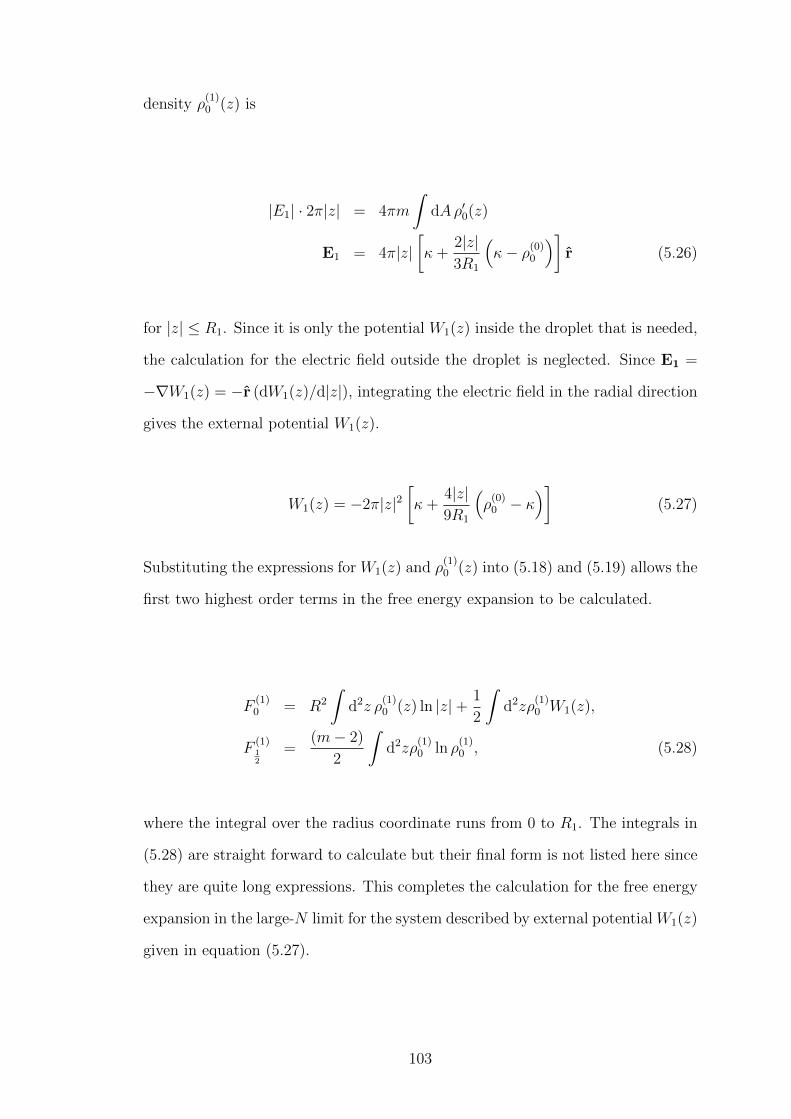
density ρ(1)0 (z) is
|E1| · 2π|z| = 4πm
∫dAρ′0(z)
E1 = 4π|z|[κ+
2|z|3R1
(κ− ρ(0)
0
)]r (5.26)
for |z| ≤ R1. Since it is only the potential W1(z) inside the droplet that is needed,
the calculation for the electric field outside the droplet is neglected. Since E1 =
−∇W1(z) = −r (dW1(z)/d|z|), integrating the electric field in the radial direction
gives the external potential W1(z).
W1(z) = −2π|z|2[κ+
4|z|9R1
(ρ
(0)0 − κ
)](5.27)
Substituting the expressions for W1(z) and ρ(1)0 (z) into (5.18) and (5.19) allows the
first two highest order terms in the free energy expansion to be calculated.
F(1)0 = R2
∫d2z ρ
(1)0 (z) ln |z|+ 1
2
∫d2zρ
(1)0 W1(z),
F(1)12
=(m− 2)
2
∫d2zρ
(1)0 ln ρ
(1)0 , (5.28)
where the integral over the radius coordinate runs from 0 to R1. The integrals in
(5.28) are straight forward to calculate but their final form is not listed here since
they are quite long expressions. This completes the calculation for the free energy
expansion in the large-N limit for the system described by external potential W1(z)
given in equation (5.27).
103

5.2.3 Free Energy Expansion with Potential W2(z)
In this section, the free energy expansion is calculated analytically for some config-
uration of charges of a one-component plasma described by the external potential
W2(z). The charges are confined to some droplet originating in the center of the
complex plane. This region of charge is denoted as the domain D2. The external
potential W2(z) is related to the density of charges when the system is in its equi-
librium configuration; this density is denoted as ρ(2)0 (z). This density is chosen to
be convenient when performing a MC simulation on the system and has the form
ρ(2)0 (z) = κ+
(ρ
(0)0 − κ
)√ |z|R2
. (5.29)
Again ρ(0)0 = 1/(πm) and κ is a small deviation of this value. This density profile
is sketched in Figure 5.2.
The radius of the droplet of charges R2 confined to domain D2 is calculated such
that
∫d2zρ
(0)0 (z) ≡
∫d2zρ
(2)0 (z), (5.30)
which gives the radius R2 in terms of the of the radius R for the uniform charge
distribution,
R2 = R
√√√√ 5
2π(κ+ 4ρ
(0)0
) . (5.31)
Following the method to extract the form of the external potential as described in
Section 5.2.2 the external potential W2(z) is calculated to be
104
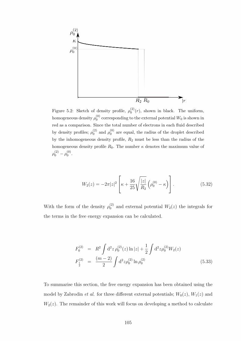
Figure 5.2: Sketch of density profile, ρ(2)0 (r), shown in black. The uniform,
homogeneous density ρ(0)0 corresponding to the external potentialW0 is shown in
red as a comparison. Since the total number of electrons in each fluid described
by density profiles; ρ(2)0 and ρ
(0)0 are equal, the radius of the droplet described
by the inhomogeneous density profile, R2 must be less than the radius of the
homogeneous density profile R0. The number κ denotes the maximum value of
ρ(2)0 − ρ
(0)0 .
W2(z) = −2π|z|2κ+
16
25
√|z|R2
(ρ
(0)0 − κ
) . (5.32)
With the form of the density ρ(2)0 and external potential W2(z) the integrals for
the terms in the free energy expansion can be calculated.
F(2)0 = R2
∫d2z ρ
(2)0 (z) ln |z|+ 1
2
∫d2zρ
(2)0 W2(z)
F(2)12
=(m− 2)
2
∫d2zρ
(2)0 ln ρ
(2)0 (5.33)
To summarise this section, the free energy expansion has been obtained using the
model by Zabrodin et al. for three different external potentials; W0(z), W1(z) and
W2(z). The remainder of this work will focus on developing a method to calculate
105

the free energy exactly for each of these potentials such that the first couple of
terms in the free energy expansion by Zabrodin et al. can be compared. The
numerical procedure used for the exact free energy expansion will be discussed in
Section 5.3.
5.3 Numerical Calculation of the Free Energy
In Eq. (5.4) the free energy expansion is shown to be related to the partition
function ZN in the following way,
F
~2= lnZN = C(N) +
F0
~2+F 1
2
~. (5.34)
To test the accuracy of this expansion a MC calculation can be used by computing
the ratio of the partition functions of the two systems for various values of N .
eτ(i)mc =
Z(i)N
Z(0)N
=
∫ N∏k=1
(d2zk e
Wi(zk)/~) N∏i<j
|zi − zj|2m
∫ N∏k=1
(d2zk e
W0(zk)/~) N∏i<j
|zi − zj|2m, (5.35)
where W0 = −zz and i = 1, 2 which corresponds to either the potential W1 or W2.
Therefore the formula (5.4) is tested by comparing the difference of two different
free energy expansions in the large N limit.
It is straightforward to see that the numerically computed value of τ(i)mc in Eq.
(5.35) should be equivalent to the value of τ(i)wz given by
τ (i)wz = lnZ
(i)N − lnZ
(0)N (W ) =
(mN
R2
)2
(F(i)0 − F
(0)0 ) +
mN
R2(F
(i)12
− F (0)12
), (5.36)
106
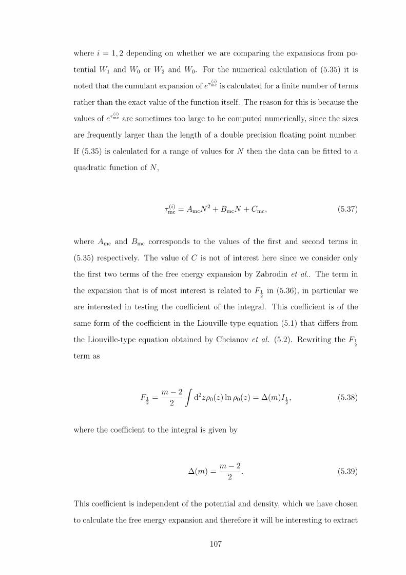
where i = 1, 2 depending on whether we are comparing the expansions from po-
tential W1 and W0 or W2 and W0. For the numerical calculation of (5.35) it is
noted that the cumulant expansion of eτ(i)mc is calculated for a finite number of terms
rather than the exact value of the function itself. The reason for this is because the
values of eτ(i)mc are sometimes too large to be computed numerically, since the sizes
are frequently larger than the length of a double precision floating point number.
If (5.35) is calculated for a range of values for N then the data can be fitted to a
quadratic function of N ,
τ (i)mc = AmcN
2 +BmcN + Cmc, (5.37)
where Amc and Bmc corresponds to the values of the first and second terms in
(5.35) respectively. The value of C is not of interest here since we consider only
the first two terms of the free energy expansion by Zabrodin et al.. The term in
the expansion that is of most interest is related to F 12
in (5.36), in particular we
are interested in testing the coefficient of the integral. This coefficient is of the
same form of the coefficient in the Liouville-type equation (5.1) that differs from
the Liouville-type equation obtained by Cheianov et al. (5.2). Rewriting the F 12
term as
F 12
=m− 2
2
∫d2zρ0(z) ln ρ0(z) = ∆(m)I 1
2, (5.38)
where the coefficient to the integral is given by
∆(m) =m− 2
2. (5.39)
This coefficient is independent of the potential and density, which we have chosen
to calculate the free energy expansion and therefore it will be interesting to extract
107

this value from the numerical data computed from the MC simulation. According
to (5.37) and (5.38) the numerical value of ∆(m) is given by
∆mc(m) =BmcR
2
m(I(1)12
− I(0)12
). (5.40)
In this section we have described a method in which the large N , free energy
expansion predicted by Zabrodin et al. can be tested and in particular we are
interested in testing the value of ∆(m) which according to the model has a value
given by Eq. (5.39).
5.4 Simulation Details
In total, 12 MC computations have been performed; for convenience each compu-
tation is denoted as τ(i)mc(κ,m). The symbol i represents whether the difference in
the free energy expansion is between W1(z) and W0(z) (i = 1) or W2(z) and W0(z)
(i = 2). κ denotes the magnitude of the density ρ(i)0 at the value z = 0 and can
have the value κ1 = ρ(0)0 + 1/4πm or κ2 = ρ
(0)0 + 1/10πm, where ρ
(0)0 = 1/(πm).
Then m corresponds to the value of the inverse filling in the FQHE terminology for
which τ(i)mc(κ,m) was computed for m = 1, 2, 3. The MC simulations to calculate
(5.35) were run for different particle number N , starting at N = 50 particles all the
way to N = 140 particles and the value of the constant radius R was chosen to be
R =√
2m50 and is therefore chosen to be dependent on the value of m. The rea-
son for testing the expansions for two different values of κ was to investigate if the
behaviour of the cumulant expansion strongly depended on the magnitude of the
alteration of the density from the uniform density value, i.e., |κ−ρ(0)0 |. In the next
section the results of all simulations listed here are presented and then compared
to the predicted results from the analytic model of the free energy expansion.
108
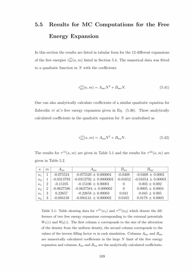
5.5 Results for MC Computations for the Free
Energy Expansion
In this section the results are listed in tabular form for the 12 different expansions
of the free energies τ(i)mc(κ,m) listed in Section 5.4. The numerical data was fitted
to a quadratic function in N with the coefficients
τ (i)mc(κ,m) = AmcN
2 +BmcN. (5.41)
One can also analytically calculate coefficients of a similar quadratic equation for
Zabrodin et al.’s free energy expansion given in Eq. (5.36). These analytically
calculated coefficients in the quadratic equation for N are symbolised as
τ (i)wz (κ,m) = AwzN
2 +BwzN. (5.42)
The results for τ (1)(κ,m) are given in Table 5.1 and the results for τ (2)(κ,m) are
given in Table 5.2.
κ m Awz Amc Bwz Bmc
κ1 1 -0.075524 -0.075520 ± 0.000004 -0.0408 -0.0408 ± 0.0003κ2 1 -0.0313793 -0.0313792 ± 0.0000003 -0.01652 -0.01654 ± 0.00003κ1 2 -0.15105 -0.15106 ± 0.00001 0 0.003 ± 0.002κ2 2 -0.0627586 -0.0627584 ± 0.000002 0 0.0005 ± 0.0004κ1 3 0.22657 -0.22658 ± 0.00003 0.041 0.045 ± 0.005κ2 3 -0.094138 -0.094141 ± 0.000002 0.0165 0.0178 ± 0.0003
Table 5.1: Table showing data for τ (1)(κ1) and τ (1)(κ2) which denote the dif-
ference of two free energy expansions corresponding to the external potentials
W1(z) and W0(z). The first column κ corresponds to the size of the alteration
of the density from the uniform density, the second column corresponds to the
values of the inverse filling factor m in each simulation. Columns Amc and Bmc
are numerically calculated coefficients in the large N limit of the free energy
expansion and columns Awz and Bwz are the analytically calculated coefficients.
109

κ m Awz Amc Bwz Bmc
κ1 1 -0.051707 -0.051707 ± 0.000001 -0.02477 -0.02477 ± 0.00008κ2 1 -0.0211961 -0.0211961 ± 0.000001 -0.00997 -0.00997 ± 0.00001κ1 2 -0.103413 -0.103410 ± 0.000008 0 0.000 ± 0.001κ2 2 -0.0423922 -0.0423928 ± 0.0000007 0 0.0004 ± 0.0001κ1 3 -0.155120 -0.155125 ± 0.000007 0.025 0.027 ± 0.001κ2 3 -0.0635883 -0.0635899 ± 0.0000005 0.00997 0.01070 ± 0.00008
Table 5.2: Table showing data for τ (2)(κ1) and τ (2)(κ2) which denote the dif-
ference of two free energy expansions corresponding to the external potentials
W2(z) and W0(z). The structure of this table is identical to Table 5.1.
From the results in Table 5.1 and Table 5.2, there is a good fit for the free energy
expansion model formulated by Zabrodin et al. and the numerical simulations for
the free fermion case. The results for m = 2 and m = 3 however are questionable.
In general the coefficient of the quadratic term in N , Awz can be matched to
the numerical data in the m = 2 case, though there is some deviance from the
expected value for m = 3. For the coefficient of the linear term in N , labelled Bwz,
there could be a fit for the m = 2 case, since the magnitude of the error in the
MC simulations is the same order of the measurement of Bwz, implying that this
result is zero within the confines of the simulation. The results which show a clear
deviance from the predicted values of the free energy model are measurements on
Bwz for m = 3. In Table 5.3 the values for ∆(m) have been listed for all of the 12
simulations carried out so far. From the free energy expansion model, the value
of ∆(m) is given in (5.39) and it can be extracted from the numerical data as
described in (5.40).
As expected, the data for the free fermion case m = 1 agree with the model
values for ∆(1). The results for m = 2 are unclear, and this is a consequence of
attempting to measure an observable whose value is obviously very small. Results
for ∆(3) appear not to match the predicted value from the model, in particular
all the numerical values from the four simulations run for this FQH filling factor
point at the value ∆(3) = 0.54 rather than 0.50, which is the model value.
110

m Model τ (1), κ1 τ (1), κ2 τ (2), κ1 τ (2), κ2
1 −12
-0.500 ± 0.004 -0.5004 ± 0.0009 -0.50 ± 0.01 -0.5003 ± 0.00072 0 0.04 ± 0.02 0.02 ± 0.01 0.00 ± 0.02 0.020 ± 0.0053 1
20.55 ± 0.06 0.54 ± 0.01 0.54 ± 0.02 0.537 ± 0.004
Table 5.3: Table summarising the values calculated for ∆(m). The first col-
umn corresponds to the value for the inverse filling factor m. The second
column is the value of ∆(m) from the analytic free energy expansion. The last
four columns corresponds to the numerical ∆(m) values from all simulations;
τ (1)(κ1), τ (1)(κ2), τ (2)(κ1) and τ (2)(κ2).
5.6 Summary and Conclusion
Clearly, the results listed in the previous section do not all match the prediction
by Zabrodin et al. for the free energy expansion in the large N limit. For FQH
filling factor m = 1, there is a good match between the analytic data and numerical
simulations which is not surprising since the free fermion case can be solved exactly
using analytic methods. What the numerical results do show for this case, is that
the method used in the MC simulations can work for this model. For m = 2, the
results are generally inconclusive due the values of the observables measured in
the MC simulation being small in magnitude. MC obviously struggles to calculate
such small observables due to the errors produced by the simulation. For the
m = 3 case there is certainly a deviance from the model predictions of the value
for ∆(m), this is clear since all four simulations run for this filling factor tend to
the same value of 0.54.
In general the numerical results do a agree with the behaviour of ∆(m) in the sense
that for m = 1, the value is negative, gets closer to zero for m = 2, then becomes
larger and positive for m = 3. Further testing needs to be carried out to accurately
pinpoint what has caused the differences between the numerical data and the model
values of the free energy expansion in the large N limit. A possibility to account
for these discrepancies is that they are caused by boundary effects that are not
taken into consideration in the work by Zabrodin et al. For example in the two
111

systems where the free energy expansion has been numerically tested, described
by the external potentials W1(z) and W2(z), the density profile has been altered
such that the radius of these systems has been shifted by an amount as compared
to the radius of the FQH system described by the external potential W0(z) = zz.
Also close to the boundary, the value of the density is different from the value of
the FQH system where the density is ρ(0)0 = 1/(πm).
Such boundary effects can be removed by considering a potential W3(z) such that
R3 = R and for a few magnetic lengths from the boundary, ρ(3)0 = ρ
(0)0 . This
investigation is ongoing. Another avenue of investigation is by directly testing the
forms of the Liouville-type equations themselves. In particular both Cheianov et
al.’s equation (5.2) and Zabrodin et al.’s equation (5.1) can be solved for ρ0(z) an-
alytically for some external potential W (z). These solutions can then be compared
to numerical computations of the density ρ0(z) from a MC simulation.
In summary, the analytic formula for the large N expansion obtained by Zabrodin
et al. has been tested via a microscopic computation. The numerical method of
performing the calculation is MC. To carry out the tests, specific systems were
chosen, where the density profile has been purposefully manipulated to deviate
from the constant, homogeneous density profile of charges observed in systems
such as the FQHE. This allowed the difference of the free energy expansions to be
calculated for the perturbed density profile and the constant density profile using
MC. The predictions for the free energy expansion obtained by Zabrodin et al.
does not match numerical data for m = 3, and, possibly m = 2. Further testing is
being carried out to identify the causes of these differences between the numerical
computations and the analytic model.
Even though there is not an exact match between Zabrodin et al.’s predictions
and the free energy expansion, what the results in this chapter do imply is that
Zabrodin et al.’s Liouville-type equation is more likely to predict more accurate
description of the equilibrium charge density of a QH fluid subject to an external
112

potential, rather than the Liouville-type equation derived by Cheianov et al. This
statement can be made in light of the behaviour of ∆(m) as shown in Table 5.3,
though a more thorough investigation is needed before any definite conclusions can
be stated. Experimentally accurate measurements at QPC’s in the FQHE could
also potentially help to resolve which description of the equilibrium charge density
works best. The main technicality here, from the theoretical perspective, would
be finding an external potential to solve the Liouville-type equations that matches
the external potential in the experiment to sufficient accuracy.
113
Chapter 6
Summary, Conclusions, and
Future Work
The aim of the work covered in this thesis was to microscopically verify effective
theory predictions with regards to the FQHE. Throughout this thesis only FQH
states described by the Laughlin wavefunction have been considered. These states
were introduced in Chapter 1; they lie in the LLL and have filling factors of the form
ν = 1/m, where m is an odd integer. The edge states in FQH systems support low-
energy excitations and they determine how charge is transported throughout the
system. There exists a phenomenological description of these edge states provided
by Wen. This is the chiral Luttinger liquid theory and it has been successful
in making predictions on transport behaviour, which can be tested and verified
experimentally. The chiral Luttinger liquid was discussed in detail in Chapter 3
where the bosonised formula for the electron fields were formulated by performing
a projection onto the low-energy space of excitations.
Original work was also presented in Chapter 3, Section 3.3 with regards to the
overlap of Laughlin states supporting low-energy excitations. An analytic for-
mula for the overlap of states for a single edge system was originally derived by
Cheianov et al. [94], as discussed in Section 3.2. This formula uses the tau-
114

function τ ν(N,M, tk, tk) to calculate overlap matrix elements. In Appendix B this
tau-function was derived for a two-edged system following a boson field theory
method originally discussed in [98]. Using the tau-function, τ ν(N,M, t±k, t±k) for
both inner and outer boundary edge excitations, allows the formula for the overlap
of states derived by Cheianov et al. to be extended to a two-edged FQH system.
This formula was important to verify since, firstly; the microscopic calculations in
the large N limit have never been extensively investigated. Secondly, the method
used to obtain the tau-function in Appendix B relies on a boson field theory
created using the grand partition function. Therefore the states that are averaged
over in this field theory, not only are dependent on the energy of the system, but
also the number of particles. Such an average for bulk properties of the FQH
system should not be affected by including states of varying number of particles,
however boundary specific properties such as the tau-function, could possibly be
affected. The microscopic definition of the tau-function (i.e. the norm of the
Laughlin wavefunction with the addition of edge excitations) is for a constant
particle number. By verifying the formula for the overlap of states, the form of
the tau-function is also checked.
To verify the analytic formula for the overlap of Laughlin states containing edge ex-
citations, the microscopic formulas were computed using the Monte Carlo method.
The space of states used in the computation were restricted such that the angu-
lar momentum contributions from the edge excitations on the inner and outer
boundary were given by 2 or 0 in units of ~. The Monte Carlo procedure was the
subject of Chapter 2 and it was shown that the numerical method could be used
effectively for computing FQHE observables due to the correspondence between
the Laughlin state and the partition function of a one component plasma. The
MC data for the microscopic computations for the overlap integrals were in good
correspondence to the predictions from the analytic formula, and thus also the
form of the tau-function for a two-edged system was also verified.
115

A particular transport property of the FQHE that was studied in this thesis was
the tunnelling of charge particles across the incompressible bulk states of a two-
edged FQH device. The motivation for such an investigation was the lack of a
microscopically derived theory. The description of tunnelling that is commonly
used in the FQHE is an effective tunnelling operator built up from the bosonised
operators defined in the chiral Luttinger liquid theory. Existing literature using
the effective tunnelling Hamiltonian was discussed in detail in Section 1.5. The
main concerns about the effective theory tunnelling operator was that it was taken
from the description of tunnelling for a conventional Luttinger liquid and directly
applied to a chiral Luttinger liquid describing the edge states of the FQHE.
Such an assumption has possible issues because, firstly, in a conventional Luttinger
liquid, the bosonised fermion fields can be microscopically derived unlike for simi-
lar fields in the chiral Luttinger liquid, which are obtained from a projection onto
the FQH low-energy edge states. This can lead to an issue with locality of the tun-
nelling operator in the FQHE. The second potential issue is that in a conventional
Luttinger liquid, interactions can be treated as perturbations whereas switching
off interactions in the FQHE is impossible because the system only exists in the
presence of strongly correlated electrons.
The need to describe the tunnelling process in the FQHE with an effective theory
is a consequence of the microscopic picture being difficult to analytically solve for
large system sizes. This was discussed in Section 3.1; therefore for microscopic
computations concerning tunnelling in the FQHE, the MC method would have to
be used.
The comparison of the effective theory and the microscopic representation of tun-
nelling in the FQHE was carried out In Chapter 4. To make the comparison,
the zero mode tunnelling matrix elements in the microscopic picture were first
formulated. These tunnelling matrix elements corresponded to some amount of
charge being transferred from the outside edge of a disk of FQH fluid to the inside
116
edge due to an impurity inserted into the bulk of the quantum fluid. To compute
these microscopic matrix elements using MC, a phase problem had to first be re-
solved. In this thesis two methods were found to solve this problem. The first
method was to calculate the cumulant expansion of the matrix elements rather
than the exact function itself. This method was appropriate when considering a
single quasiparticle tunnelling between the edge states. The second method found
was for an electron tunnelling across the bulk states. In this special case, due to
angular momentum considerations the integrals describing the tunnelling process
of an electron could be transformed purely in terms of real functions, thus remov-
ing any phase problems encountered in the MC simulations. The details of these
methods were given in Section 4.1.
The effective theory zero mode tunnelling operators were then calculated in Section
4.2 using the operators from the chiral Luttinger liquid theory. It was found that
one specific type of ordering of the operators in the effective tunnelling Hamiltonian
lead to a local tunnelling operator. The results for the local tunnelling operators
were chosen to be compared with the microscopically computed tunnelling matrix
elements. The comparison between the effective and microscopic theories was made
by comparing the size dependence of the zero mode tunnelling matrix elements.
The specific Laughlin states that were considered in this work correspond to the
filling factors ν = 1 and ν = 1/3.
The calculations using the local tunnelling operator were found to be in good agree-
ment with the MC data for electron tunnelling in both the ν = 1 and ν = 1/3
QH state. However, the effective theory tunnelling Hamiltonian for a Laughlin
quasiparticle did not predict the same scaling behaviour as computed microscop-
ically for the tunnelling matrix elements. This result was found for FQH filling
factor ν = 1/3 and could hint at there being an error within the effective theory.
To confirm this assertion, the scaling behaviour for the quasiparticle tunnelling
matrix elements in other Laughlin states, such as ν = 1/5, 1/7, etc., should also
117

be investigated, as well as the tunnelling processes for multiple quasiparticles at
the impurity. Such findings will hint as to where possible sources of the errors
occur in the effective theory of tunnelling across the bulk FQHE.
Definite conclusions that were drawn from Chapter 4 was that the bosonised oper-
ator ordering in the tunnelling Hamiltonian is important and must be considered
when performing calculations related to tunnelling in the FQHE. Changing the
ordering of the bosonised operators effects the locality of the tunnelling opera-
tor. Another important finding from the microscopic computations of both the
quasiparticle and electron tunnelling matrix elements for ν = 1/3 was that the
electron tunnelling process is less relevant than the quasiparticle tunnelling pro-
cess for all system sizes. This validates tunnelling calculations, which disregard
the electron tunnelling operator in the effective tunnelling Hamiltonian in favour
of only considering the quasiparticle tunnelling process.
With the success of the MC method to perform microscopic computations in the
FQHE, in Chapter 5 a similar numerical procedure was performed, but now mea-
suring the effective free energy of the system. The motivation for this project
is related to the fact that there exists conflicting results between the work by
Zabrodin et al. and Cheianov et al. Both have derived a Liouville-type equation
in the semi-classical limit for the equilibrium density in terms of some background
potential. The methods used are quite different, and as a consequence the Liou-
ville equation derived by Cheianov et al. differs to the equivalent equation derived
by Zabrodin et al. Therefore the aim of the work discussed in Chapter 5 was
to check which Liouville equation most accurately described the behaviour of the
FQH fluid. The method used by Cheianov et al. is discussed in Appendix B.1.
To perform a check for the two different Liouville equations, it was noticed that
Zabrodin et al. had also derived a free energy expansion in the large N limit, where
N corresponds to the number of electrons. The free energy is just the logarithm
of the partition function or, using the plasma analogy, the magnitude squared of
118
the wavefunction. From Chapter 2 and Chapter 4 objects such as the norm of
the Laughlin wavefunction are easily computed using MC, thus the free energy
expansion was chosen to be tested microscopically, which in turn would shed light
on the accuracy of the Liouville equation derived by Zabrodin et al. In particular,
the two Liouville equations differ only in a single coefficient. For the Liouville
equation derived by Zabrodin et al. this coefficient is denoted ∆(m) and the same
coefficient also appears in the free energy expansion. Therefore it is of particular
interest to compute the value of ∆(m) from the MC simulations.
In Section 5.2 analytic expressions for the free energy expansions were calculated
for two background potentials in accordance with the formulae from Zabrodin et
al.’s work. These expressions could in turn be compared to the MC data, which
were obtained using the cumulant expansion method. The FQH states used in
the MC simulations corresponded to filling factors ν = 1, 2, and 3. In the free
fermion case (m = 1) the MC data was in complete agreement with the large N
expansion of the free energy obtain by Zabrodin et al. For m = 2, the MC data
was inconclusive. The reason for the lack of clear data for this filling factor was
due to the measured values from the MC simulations being small in magnitude,
thus they were obscured by intrinsic statistical errors of the MC program. Finally
for the inverse filling factor m = 3, the MC results suggest that the value of ∆(m)
was not the same as the predicted value from the free energy expansion model.
The numerical results consistently gave a value closer to 0.54, whereas the model
predicts ∆(m) = 0.50.
It was deduced that the discrepancy from the m = 3 simulations were not a
consequence of the MC method used, I.e. it was not a systematic error of the
cumulant expansion since no significant systematic error was apparent in the free
fermion simulation. However it could be a result of boundary effects that are not
taken into account in the model of the free energy expansion by Zabrodin et al.
This project is still ongoing.
119
At the end of both the Chapters 4 and 5 there have already been proposals made
for further areas of study. For Chapter 5 which was concerned with the large N
expansion of the free energy, further MC tests were proposed which remove all
boundary effects from the problem. Such a simulation should be a better match
for the free energy expansion by Zabrodin et al. since their model does not take
into account perturbations around the boundary.
Another proposal for further study is directly related to the Liouville equations
derived by Cheianov et al. and Zabrodin et al. Both equations could be solved an-
alytically for some background potential. To investigate which Liouville equation
gives the most accurate equilibrium density distribution the analytical solutions
can be compared to a MC simulation of the same background potential which
calculates the density at given positions in the quantum fluid.
With regards to further work for the testing of the effective tunnelling Hamiltonian
in Chapter 4, it was proposed that the occupied angular momentum orbitals could
be increased such that we are no longer considering solely the zero mode matrix
elements. The problem with this is the vast number of states and therefore MC
simulations that would have to be included for an analysis that considers tunnelling
of excitations between one occupied orbital on one boundary to a different orbital
on the adjacent boundary. If an angular momentum cutoff is imposed however
this is possible and some trial simulations have already been carried out for the
free fermion case. These preliminary results show that the MC computation is still
a good method for investigating tunnelling of higher angular momentum orbitals
since the results can be checked against an exact analytic calculation for m = 1.
The method to calculate the analytic solution is discussed in Appendix A.2.
In Chapter 4 only tunnelling for Laughlin states was considered. In reality there
are many other FQH states that cannot be described by this wavefunction. An
example is the state with filling factor ν = 5/2. It was mentioned in Section 1.5
that not only is the microscopic wave function that describes this state unknown,
120

but whether the system follows Abelian or non-Abelian fractional statistics is still
under debate. One proposal for a possible wavefunction for the ν = 5/2 state is
the Pfaffian wave function. This state supports non-Abelian fractional statistics
and recently it has been indicated that there may also exist a plasma analogy for
the Pfaffian state [102]. With a plasma analogy for the Pfaffian state a similar
set of MC computations for tunnelling matrix elements can be carried out which,
in turn can be compared to both the effective theory predictions for this wave
function and also to experimental results measuring the tunnelling currents. Such
simulations would shed light on the microscopic representation of this ν = 5/2
state.
The final avenue to be considered for future study is related to the Klein fac-
tors, originally discussed in Section 1.5. Klein factors are extra phases added to
the quasiparticle operators in the chiral Luttinger liquid theory. These phases
allow multiple tunnelling operators at spatially separated multiple QPC’s to com-
mute with each other. Without these phases the tunnelling operators would not
commute and thus be non-local operators. The addition of these Klein factors in
literature is justified as being a manifestation of the fractional statistics followed by
the quasiparticles. It is known from the chiral Luttinger liquid theory that for two
quasiparticles exchanged on the same edge, a phase is obtained as a consequence
of the fractional statistics. The Klein factors are obtained from the conjecture
that a similar phase should also be picked up from exchanging quasiparticles on
two disconnected edges (such as the inner and outer boundary of the FQH disk
geometry considered in this thesis). An investigation to see if these Klein factors
manifest from the microscopic theory would be extremely interesting. They have
not been explicitly probed in the work presented in Chapter 4, concerned with
the zero mode tunnelling matrix elements for the disk FQH device since it can
be reasoned that for a two-edged system, the Klein factors do not contribute to
observables [63]. Thus a system of three or more disconnected edges would have
to be modelled microscopically.
121

In this thesis the MC method has been used to test the accuracy of effective
theories for Laughlin FQH fluids. For MC simulations to be accurate and have a
quick convergence, two solutions have been proposed to overcome phase problems
that occur whilst considering tunnelling in Laughlin FQH systems. In particular
using the results obtained from MC computations, it has been shown that the
effective theory of electron tunnelling is an accurate description of the processes
computed microscopically. This result is only true for a specific ordering of the
chiral Luttinger liquid operators in the effective tunnelling Hamiltonian. Using this
operator ordering also makes the Hamiltonian a local operator. The agreement
between the microscopic computation and effective tunnelling Hamiltonian does
not extend however, for a quasiparticle tunnelling across the bulk of the QH fluid,
in the state ν = 1/3. The cause of this disagreement may possibly be caused by an
inaccuracy in the effective quasiparticle tunnelling Hamiltonian. The MC method
has also been used to attempt to resolve the accurate form of the Liouville-type
equation for the equilibrium density of a Laughlin quantum fluid. Overall the
data was inconclusive possibly due to boundary effects in the simulation that were
not considered in the analytic model, which the numerical data was compared to.
Proposals have been made to overcome these boundary effects and work is still
ongoing to resolve which Liouville-type equation best describes the equilibrium
density distribution of a FQH system.
122

Appendix A
Theory of Symmetric Functions
and the Free Fermion QHE
In Section A.1 of this appendix, a brief overview of the theory of symmetric poly-
nomials is given. This material is complimentary to discussions in Section 3.1
of Chapter 3. Section A.2 contains information for analytically calculating exact
overlap integrals for the free fermion QHE. Such methods have been used as a
check for all MC programs discussed in this thesis.
A.1 Introduction to the Theory of Symmetric
Polynomials
Good references for the theory of symmetric polynomials can be found in books
[103] and [104]. This section introduces some definitions of the theory of symmetric
polynomials. A polynomial P (z1, z2, ..., zN) is symmetric if it is left invariant under
any transformation permuting any of the zi variables. Symmetric polynomials can
be expressed as a sum of monomial symmetric functions defined via;
123

mλ =∑P
zλ11 zλ2
2 zλ33 .....zλNN (A.1)
where the sum is over all permutations P of the coordinates {zi}. Therefore
monomial symmetric functions form a linear basis for all symmetric polynomials.
Different monomial symmetric functions can be distinguished from one another
via their relationship to a partition. A partition is an ordered set of integers which
can be written as,
λ = {λ1, λ2, λ3, ...., λN}, (A.2)
where λi are all integers and λ1 ≥ λ2 ≥ .... ≥ λN . Therefore the monomial given in
Eq. (A.1) has the subscript λ, which refers to the partition, and the powers of the
coordinates in the right-hand-side of the expression correspond to the integers in
the partition itself. For example, for the number of variables N = 3, the symmetric
monomial function corresponding to the partition λ = {3, 2, 1} is
mλ = z31z
22z
13 + z3
1z12z
23 + z2
1z32z
13 + z2
1z12z
33 + z1
1z32z
23 + z1
1z22z
33 . (A.3)
and we see from (A.3), the symmetric monomial functions are permanents.
The weight of a partition |λ| is defined as |λ| = λ1 + λ2 + λ3 + ......+ λN and the
length l(λ) is the number of parts, or integers the partition contains. For example
in (A.2), we have l(λ) = N . For meaningful partitions with regards to FQH
systems, it is required that l(λ) is less than or equal to the number of variables
zi. Another notation that is frequently used inside the partition is, kmk where
mk denotes the multiplicity, or frequency with which the integer k occurs. For
example;
124

λ = {31, 21, 13} = {3, 2, 1, 1, 1}. (A.4)
It will be shown that these two representations of the partition correspond to either
the boson or fermion representation of the low-energy excitations in the Laughlin
wavefunction. There are three main types of symmetric polynomials that we are
concerned with initially, these are;
1. Elementary symmetric functions,
2. Homogeneous product sums,
3. Power sums.
1. Elementary Symmetric Functions
For a total of N variables, the elementary symmetric functions are defined as
follows;
a1 =∑P
z1
a2 =∑P
z1z2
a3 =∑P
z1z2z3
...
an =∑P
z1z2z3.....zn (A.5)
where the sum is over all permutations of the N variables. For example, when
N = 3 the first three elementary symmetric functions are the following.
125

a1 = z1 + z2 + z3
a2 = z1z2 + z2z3 + z1z3
a3 = z1z2z3 (A.6)
The generators of the elementary symmetric functions are;
f(x) =n∏i=1
(1− zix) = 1− a1x+ a2x2 − a3x
3 + .....+ (−1)nanxn. (A.7)
2. Homogeneous Product Sums
The generator for the homogeneous product sums hi is simply the inverse of f(x)
in Eq. (A.7);
1
f(x)=
1
1− a1x+ a2x2...+ (−1)nanxn
= 1 + h1x+ h2x2 + h3x
3 + ....+ hnxn + ... (A.8)
where the last equality arises from an expansion of x. To obtain an expression for
the homogeneous product sums in terms of the variables zi, one can expand the
inverse of the product in (A.7) to give,
1
f(x)=∏i=1
(1 + zix+ z2
i x2 + z3
i x3 + ....
). (A.9)
Comparing the expressions in (A.8) and (A.9) we see that the homogeneous power
sums are simply the sum of all monomial symmetric functions of the same degree.
126

The first three homogeneous product sums are given below, where the sum is taken
over all permutations of the variables index.
h1 =∑P
z1
h2 =∑P
z21 +
∑P
z1z2
h3 =∑P
z31 +
∑P
z21z2 +
∑P
z1z2z3 (A.10)
3. Power Sums
Power sums, Sk are the sum over all variables to the power k.
Sk =∑P
zk1 (A.11)
The generating function for the power sum polynomials is obtained by differenti-
ating f(x) with respect to x in (A.7) then dividing the resulting function by f(x)
itself, i.e.
f ′(x)
f(x)=∑i
−zi1− zix
= −S1 − S2x− S3x2 − ...− Snxn−1 − ... (A.12)
It is the power sum polynomials of the form (A.11) that can be multiplied by
the Laughlin states to describe excitations in QH edge states. To see how this is
achieved we first consider a circular droplet of Laughlin’s incompressible fluid in
the free fermion state with m = 1.
One of the first papers to highlight the advantages of describing FQH states in
terms of symmetric polynomials was written by Stone [87, 105]. This work focused
127

on the free fermion picture corresponding to filling factor ν = 1. The holomorphic
representation (where exponential factors are omitted) of the Laughlin wavefunc-
tion in the free fermion state is
ΨGS =N∏i<j
(zi − zj). (A.13)
The wavefunction in (A.13) is actually the Vandermonde determinant which, in
matrix form is given by,
ΨGS =
∣∣∣∣∣∣∣∣∣∣∣∣∣
zN−11 zN−2
1 · · · 1
zN−12 zN−2
2 · · · 1
......
. . ....
zN−1N zN−2
N · · · 1
∣∣∣∣∣∣∣∣∣∣∣∣∣= det|zN−ts |. (A.14)
Excited edge states in the quantum Hall effect are obtained by multiplying the
ground state wavefunction by a series of power sum polynomials given in (A.11).
A general wavefunction describing low-level excitations in the edge states for the
system of free fermions is given by
Ψ =∏k>0
(N∑i
zki
)nk N∏i<j
(zi − zj), (A.15)
where k denotes the level of the excitation and nk is the number of excitations
in the k’th level. Thus creating low-level excitations increases the powers of the
zi in the polynomial part of the wavefunction. In general these excited states
should be able to be expressed in terms of a Slater determinant, where the extra
powers due to the additional edge excitations are denoted by a set of integers
λ = {λ1, λ2, λ3, ..., λN}.
128
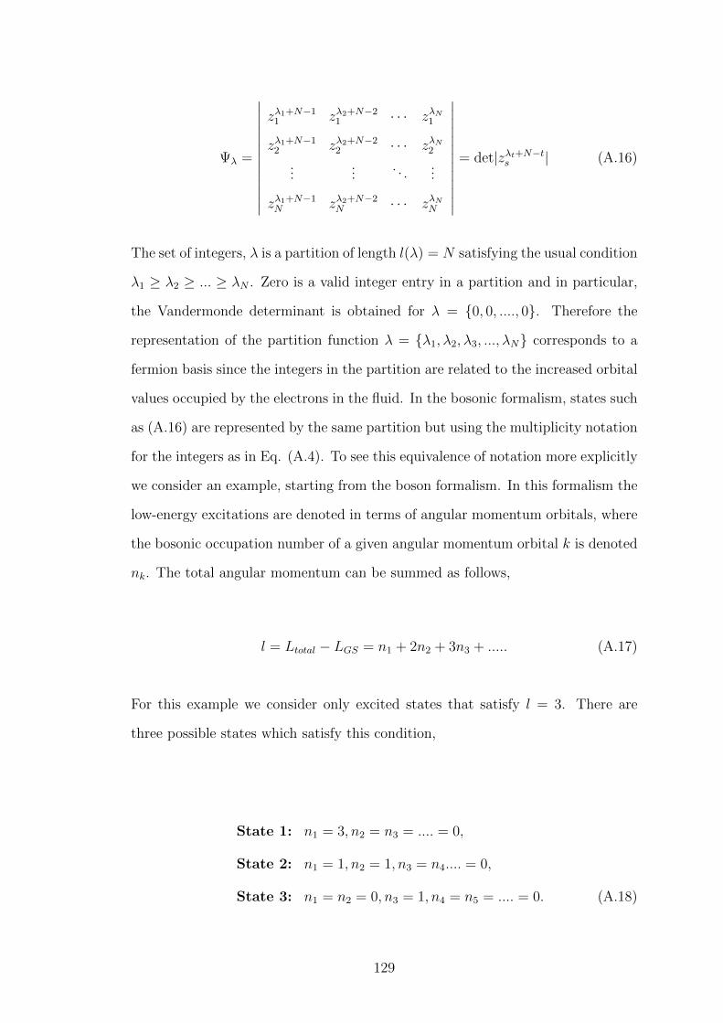
Ψλ =
∣∣∣∣∣∣∣∣∣∣∣∣∣
zλ1+N−11 zλ2+N−2
1 · · · zλN1
zλ1+N−12 zλ2+N−2
2 · · · zλN2
......
. . ....
zλ1+N−1N zλ2+N−2
N · · · zλNN
∣∣∣∣∣∣∣∣∣∣∣∣∣= det|zλt+N−ts | (A.16)
The set of integers, λ is a partition of length l(λ) = N satisfying the usual condition
λ1 ≥ λ2 ≥ ... ≥ λN . Zero is a valid integer entry in a partition and in particular,
the Vandermonde determinant is obtained for λ = {0, 0, ...., 0}. Therefore the
representation of the partition function λ = {λ1, λ2, λ3, ..., λN} corresponds to a
fermion basis since the integers in the partition are related to the increased orbital
values occupied by the electrons in the fluid. In the bosonic formalism, states such
as (A.16) are represented by the same partition but using the multiplicity notation
for the integers as in Eq. (A.4). To see this equivalence of notation more explicitly
we consider an example, starting from the boson formalism. In this formalism the
low-energy excitations are denoted in terms of angular momentum orbitals, where
the bosonic occupation number of a given angular momentum orbital k is denoted
nk. The total angular momentum can be summed as follows,
l = Ltotal − LGS = n1 + 2n2 + 3n3 + ..... (A.17)
For this example we consider only excited states that satisfy l = 3. There are
three possible states which satisfy this condition,
State 1: n1 = 3, n2 = n3 = .... = 0,
State 2: n1 = 1, n2 = 1, n3 = n4.... = 0,
State 3: n1 = n2 = 0, n3 = 1, n4 = n5 = .... = 0. (A.18)
129

To each unique state corresponds a unique partition. The integers in the partition
are given by k, where k corresponds to the occupied level of the excitation and if
nk ≥ 1, the multiplicity of k in the partition is equal nk. In general,
λ = {rnr , ..., 3n3 , 2n2 , 1n1} (A.19)
Thus our bosonic basis can be written in terms of the partitions;
λB,1 = {13}
λB,2 = {21, 11}
λB,3 = {31} (A.20)
For each bosonic excitation, the Laughlin wavefunction gets multiplied by a power
sum polynomial of degree corresponding to the momentum orbital occupied in
this representation. Thus the corresponding wavefunctions of the partitions in
(A.20) written in terms of the occupation numbers |n1, n2, n3〉 in the holomorphic
representation are;
|3, 0, 0〉 = S31
∏i<j
(zi − zj) =
[N∑i=1
zi
]3∏i<j
(zi − zj),
|1, 1, 0〉 = S1S2
∏i<j
(zi − zj) =
[N∑i=1
zi
][N∑i=1
z2i
]∏i<j
(zi − zj),
|0, 0, 1〉 = S3
∏i<j
(zi − zj) =
[N∑i=1
z3i
]∏i<j
(zi − zj). (A.21)
The corresponding fermion representation of partitions for states 1 to 3 in (A.18)
130

are;
State 1: {1, 1, 1, 0, ..., 0},
State 2: {2, 1, 0, 0, ..., 0},
State 3: {3, 0, 0, 0, ..., 0}. (A.22)
The Slater determinants corresponding to states 1 to 3 can thus be calculated
using (A.16) with the partitions given in (A.22). Therefore to summarise this
section, definitions of various types of symmetric polynomials have been introduced
along with the concept of a partition which can be represented using two different
notations. These can be thought of as a basis in the bosonic representation, where
low-energy excitations are created by multiplying the Laughlin wavefunction by a
series of power sum polynomials, or in the fermion representation where integers
in the partition correspond to the increase of angular momentum orbitals of the
electrons in the Laughlin droplet. Although the example considered in this section
was for the free fermion case, the excitation representations can be extended for
any Laughlin state with filling factor ν = 1/m. The fermion basis is most intuitive
for the free fermion case where the holomorphic part of the Laughlin wavefunction
is a Vandermonde determinant. It is for this reason the overlap integrals for the
free fermion case have an exact analytic solution. This will be the subject of the
next section.
131

A.2 Analytical Calculations for Overlap Integrals
in the Free Fermion QHE
Overlap integrals for the free fermion state can be made trivial to solve by in-
troducing another type of symmetric polynomial, called Schur functions. Schur
functions are defined by the quotient of the Slater determinants with respect to
the Vandermonde determinant. Each partition λ corresponds to a unique Schur
function;
Φλ =Ψλ
ΨGS
=det|zλt+n−ts |
det|zn−ts |, (A.23)
where the numerator of (A.23) is a Slater determinant of the form (A.16). The
inner product of two Schur functions is only non-zero when the Schur functions
are equivalent. Thus expressing FQH states for the free fermion system in terms
of Schur functions greatly reduces computational effort for the overlap of states.
The definition for the overlap of Schur functions is;
〈Φλ′ |Φλ〉 =
∫ N∏i=1
(d2zie
−|zi|2/2) N∏i<j
|zi − zj|2Φλ′Φλ. (A.24)
Using the definition of the Schur function in (A.23) as a quotient, with denominator
as the Vandermonde determinant, then the above overlap can be expressed in terms
of the product of two determinants,
〈Φλ′ |Φλ〉 =
∫ N∏i=1
(d2zie
−|zi|2/2)
det|zλ′t+n−ts |det|zλt+n−ts |δλ′λ. (A.25)
For the above integral to be non-zero there must exist terms in the product of
the two determinants which depend only on the magnitude of the coordinate and
132

not the angle. This condition is met only when λ′ ≡ λ. The product of the two
determinants is straightforward to calculate.
〈Φλ′ |Φλ〉 = (2π)NN !N∏i=1
[2λi+N−i(λi +N − i)!
]δλ′λ (A.26)
If free fermion QH states containing low-energy excitations can be expressed in
terms of the Schur functions, applying (A.26) will give the overlap of states. To
write the states as Schur functions one can use the conversion relations between
various different types of symmetric polynomials. Since the excited states of in-
terest are just the Vandermonde determinant multiplied by a series of power sum
polynomials, the aim is to be able to write such power sum polynomials as a linear
superposition of the Schur functions.
The Schur functions have a simple expression in terms of the homogeneous product
of sums given by the following determinant;
Φλ = det|hλs−s+t|. (A.27)
If one is also able to express power sum polynomials in terms of the homogeneous
product of sums then (A.27) can be used to define a new basis for the low-energy
excitations in the free fermion QH states. To do this an intermediate step is
needed which converts power sums to elementary symmetric functions (see previous
section) via the determinant of a quasi-lower triangular matrix.
133

Sr =
∣∣∣∣∣∣∣∣∣∣∣∣∣∣∣∣
a1 1 0 0 · · · 0
2a2 a1 1 0 · · · 0
3a3 a2 a1 1 · · · 0
......
......
. . ....
rar · · · · · · · · · · · · a1
∣∣∣∣∣∣∣∣∣∣∣∣∣∣∣∣(A.28)
A similar relationship also exist between homogeneous product sums and elemen-
tary symmetric functions.
ar =
∣∣∣∣∣∣∣∣∣∣∣∣∣∣∣∣
h1 1 0 0 · · · 0
h2 h1 1 0 · · · 0
h3 h2 h1 1 · · · 0
......
......
. . ....
hr · · · · · · · · · · · · h1
∣∣∣∣∣∣∣∣∣∣∣∣∣∣∣∣(A.29)
These are all the tools needed to express the power sum polynomials as a linear
superposition of Schur functions and all that remains is a simple algebraic problem.
To show an explicit example, we will continue on the example used earlier when
the three states were considered with the angular momentum contribution due to
the excitations, l = 3. These states were given in (A.21), since there are only three
partitions possible for l = 3, there are only three Schur functions that are needed
to define the basis for all states that satisfy l = 3. The aim is to find the following
coefficients such that (A.21) is satisfied.
134

|3, 0, 0〉 =(aΦ{1,1,1} + bΦ{2,1} + cΦ{3}
)∏i<j
(zi − zj)
|1, 1, 0〉 =(dΦ{1,1,1} + eΦ{2,1} + fΦ{3}
)∏i<j
(zi − zj)
|0, 0, 1〉 =(gΦ{1,1,1} + hΦ{2,1} + kΦ{3}
)∏i<j
(zi − zj) (A.30)
Equation (A.27) is first used to express the Schur functions in terms of homoge-
neous product of sums. The results for the three Schur functions in this example
are
Φ{1,1,1} = h31 − 2h1h2 + h3,
Φ{2,1} = h1h2 − h3,
Φ{3} = h3. (A.31)
Using (A.28) and (A.29) the power sum polynomials expressed in terms of the
homogeneous product of sums have the form;
S31 = a3
1 = h31,
S1S2 = a31 − 2a2a1 = −h3
1 + 2h1h2,
S3 = a31 − 3a2a1 + 3a3 = h3
1 − 3h1h2 + 3h3. (A.32)
Comparing the above with (A.31) it can be seen that (A.30) is satisfied by the
following coefficients of the Schur functions.
135
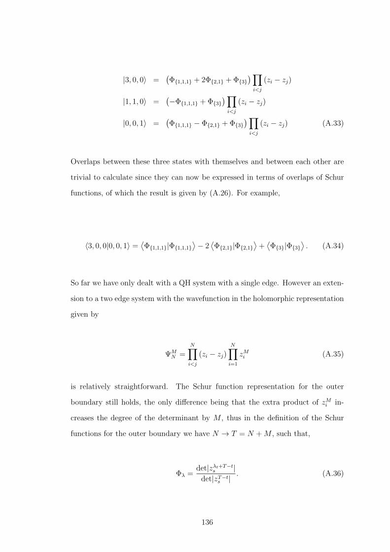
|3, 0, 0〉 =(Φ{1,1,1} + 2Φ{2,1} + Φ{3}
)∏i<j
(zi − zj)
|1, 1, 0〉 =(−Φ{1,1,1} + Φ{3}
)∏i<j
(zi − zj)
|0, 0, 1〉 =(Φ{1,1,1} − Φ{2,1} + Φ{3}
)∏i<j
(zi − zj) (A.33)
Overlaps between these three states with themselves and between each other are
trivial to calculate since they can now be expressed in terms of overlaps of Schur
functions, of which the result is given by (A.26). For example,
〈3, 0, 0|0, 0, 1〉 =⟨Φ{1,1,1}|Φ{1,1,1}
⟩− 2
⟨Φ{2,1}|Φ{2,1}
⟩+⟨Φ{3}|Φ{3}
⟩. (A.34)
So far we have only dealt with a QH system with a single edge. However an exten-
sion to a two edge system with the wavefunction in the holomorphic representation
given by
ΨMN =
N∏i<j
(zi − zj)N∏i=1
zMi (A.35)
is relatively straightforward. The Schur function representation for the outer
boundary still holds, the only difference being that the extra product of zMi in-
creases the degree of the determinant by M , thus in the definition of the Schur
functions for the outer boundary we have N → T = N +M , such that,
Φλ =det|zλt+T−ts |
det|zT−ts |. (A.36)
136

With this definition however we can obtain an overlap for the Schur functions for
the outer boundary similar to (A.26);
〈Φλ′ |Φλ〉 = (2π)NN !N∏i=1
[2λi+T−i(λi + T − i)!
]δλ′λ (A.37)
Defining a basis for excitations on the inner boundary is similar to that of the
outer boundary except now the power sum polynomials are a sum over the inverse
electron coordinate variables. Writing occupation numbers as n−k for an excitation
in the k’th orbital of the inner boundary; an example of a state containing only
inner boundary low-energy excitations is;
|n1, n2, n3〉 =
[N∑i=1
1
zi
]n−1[
N∑i=1
1
z2i
]n−2[
N∑i=1
1
z3i
]n−3 N∏i<j
(zi − zj)N∏i=1
zMi . (A.38)
A new variable can be defined, w = z−1 such that the terms defining the inner-edge
excitations are power sum polynomials in this new variable w,
Sn−k−k =
[N∑i=1
wki
]n−k=
[N∑i=1
1
zki
]n−k.
Thus, the additional angular momentum acquired by inner boundary low-energy
excitations is given by
l = Ltotal − LGS = −n−1 − 2n−2 − 3n−3 − ..... (A.39)
The definition of the Schur functions that corresponds to the inner excitations are
therefore given by;
137

Φ−λ =det|wλt+N−ts |
det|wN−ts |. (A.40)
This is the same definition as for the outer boundary excitations in Eq. (A.23) only
now the variable has changed z → w. Defining the Schur function in terms of the
variable w is however not good practice since the remainder of the wavefunction
is defined in terms of z = w−1 thus we need to convert (A.40) to an expression
dependant on z only. To begin this process, we first consider the denominator in
(A.40) and note that,
(∏i
wN−1i
)−1
det|wN−ts | = det|w1−ts | = det|zt−1
s |.
The determinant on the right-hand-side is as follows,
det|zt−1s | =
∣∣∣∣∣∣∣∣∣∣∣∣∣
1 z1 · · · zN−11
1 z2 · · · zN−12
......
. . ....
1 zN · · · zN−1N
∣∣∣∣∣∣∣∣∣∣∣∣∣.
To calculate the overlap between inner boundary Schur functions, we would hope
to be able to write the denominator in the Schur function definition (A.40) in
terms of the Vandermonde determinant in the variable z, given by;
det|zN−ts | =
∣∣∣∣∣∣∣∣∣∣∣∣∣
zN−11 · · · z1 1
zN−12 · · · z2 1
.... . .
......
zN−1N · · · zN 1
∣∣∣∣∣∣∣∣∣∣∣∣∣.
From observing the above two determinants, one can see that the Vandermonde
138

determinant det|zN−ts | can be obtained from det|zt−1s | by simply interchanging the
columns. Therefore we can now write the denominator in (A.40) in terms of the
Vandermonde determinant in variable z as
det|wN−ts | = (−1)N2
(N−1)
N∏i=1
(wN−1i
)det|zN−ts |. (A.41)
Now we focus our attention on the numerator of (A.40) proceeding in the same
way as for denominator by considering the following relation.
(∏i
wN−1i
)−1
det|wλt+N−ts | = det|wλt+1−ts | = det|zt−1−λt
s |
The form of the determinant on the right-hand-side written out explicitly is
det|zt−1−λts | =
∣∣∣∣∣∣∣∣∣∣∣∣∣
z−λ11 z1−λ2
1 · · · zN−1−λN1
z−λ12 z1−λ2
2 · · · zN−1−λN2
......
. . ....
z−λ1N z1−λ2
N · · · zN−1−λNN
∣∣∣∣∣∣∣∣∣∣∣∣∣.
One can exchange all the columns in the above determinant to completely reverse
their order which will give a factor of (−1) to the N2
(N − 1) times, this will
eventually cancel out with the same factor in (A.41).
det|zt−1−λts | = (−1)
N2
(N−1)
∣∣∣∣∣∣∣∣∣∣∣∣∣
zN−1−λN1 · · · z1−λ2
1 z−λ11
zN−1−λN2 · · · z1−λ2
2 z−λ12
.... . .
......
zN−1−λNN · · · z1−λ2
N z−λ1N
∣∣∣∣∣∣∣∣∣∣∣∣∣. (A.42)
To complete the final definition for the numerator of the Schur function, the con-
139

jugate partition λ must be defined. The partition λ = {λ1, λ2, ...., λN} can be
conjugated to give,
λ = {λ1, λ2, ..., λN−1, λN} = {λN , λN−1, ..., λ2, λ1} (A.43)
i.e., the order of the partition is simply reversed. An equation relating an element
of a partition to its conjugate element is
λN−i = λi+1. (A.44)
Using the conjugate partition λ rather than the partition λ we can express the
above determinant (A.45) as
det|zt−1−λts | = (−1)
N2
(N−1)
∣∣∣∣∣∣∣∣∣∣∣∣∣
zN−1−λ11 · · · z
1−λN−1
1 z−λN1
zN−1−λ12 · · · z
1−λN−1
2 z−λN2
.... . .
......
zN−1−λ1N · · · z
1−λN−1
N z−λNN
∣∣∣∣∣∣∣∣∣∣∣∣∣= (−1)
N2
(N−1)det|zN−t−λts |. (A.45)
So the numerator in (A.40) can be expressed as
det|wλt+N−ts | = (−1)N2
(N−1)
N∏i=1
(wN−1i
)det|zN−t−λts |. (A.46)
Combining (A.46) with (A.41), we can covert the definition of the Schur function
as a quotient in terms of w (A.40) to a simple quotient in terms of z where we
use the conjugate partition as opposed the the actual partition itself. The result
140

is given below.
Φ−λ =det|zN−t−λts |
det|zN−ts |(A.47)
All that remains is to calculate the overlap for the inner-boundary Schur functions.
〈Φ−λ′ |Φ−λ〉 =
∫ N∏i=1
(d2zie
−|zi|2/2|zi|2M) N∏i<j
|zi − zj|2Φ−λΦ−λδλ′λ
=
∫ N∏i=1
(d2zie
−|zi|2/2|zi|2M)
det|zN−t−λts |det|zN−t−λts |δλ′λ
=
∫ N∏i=1
(d2zie
−|zi|2/2)
det|zT−t−λts |det|zT−t−λts |δλ′λ,
where T = N +M . Note that this integral can only be solved when M is greater
or equal to the angular momentum contributions from the inner boundary. If this
condition is not fulfilled then negative powers of z occur in the in the determinants
for the overlap making the integrals diverge. Physically this condition makes sure
that there exists enough available excited states inside the hole of the QH disk
such that there is room for the occupancy of the inner boundary excitations.
The solution for the overlaps of the inner boundary Schur functions is as follows,
〈Φ−λ′ |Φ−λ〉 = N !(2π)NN∏i=1
(2T−i−λi(T − i− λi)!
)δλ′λ. (A.48)
Thus the inner boundary low-energy excitation states can now be treated in a
similar manner to the outer boundary excited states. The states that originally
consist of a product of power sum polynomials of the inverse variable can be
converted into a linear superposition of Schur functions defined in (A.40). The
overlap integrals for inner boundary low-energy excitations are then calculated
141

using (A.48).
The form of the overlap of Schur functions for the outer boundary and the inner
boundary allows all overlap integrals to be calculated for free fermion systems
containing any configuration of inner boundary excitations or outer boundary ex-
citations. In general, using this formalism of Schur functions in the free fermion
system, the overlap calculations of FQH excited states can be generalised to include
averages over operators.
142
Appendix B
Calculating the Norm of Laughlin
States
Laughlin-type wavefunctions are not normalised. In this section the norm of the
variational wavefunction is calculated for the generalised wavefunctions given in
(3.9), which support low-energy excitations. The norm of the wavefunctions are
tau-functions of analytic curves which have been studied in works of Wiegmann,
Zabrodin et al. [96, 97, 99]. To perform this calculation, the FQH system described
by Laughlin states is reformulated to a boson field theory using Laughlin’s plasma
analogy. The method involves expressing the grand partition function in terms of a
boson field path integral, from which an action describing the dynamics of the free
boson system can be extracted. The process that is followed here was originally
described in the work [98] for a Laughlin state containing a single edge, it has
been extended here to include excitations on the inner and outer boundaries of the
FQH device shown in Figure 1.5. The first part of this section is the field theory
reformulation for the “undeformed” Laughlin state when there are no excitations
present at the edges. In the second section the field theory formalism is extended
to include the edge excitations which in turn allows the form of the tau-function
to be calculated.
143

B.1 Boson Field Theory Reformulation for a Laughlin-
Type System
Laughlin’s plasma analogy allows one to express the magnitude squared of the
ground state wavefunction (1.31) as a partition function ZN of a classical two-
component plasma with Coulomb interactions.
ZN =
∫ N∏i
d2zie−mε =
∫ N∏i
d2zi|ΨMN |2, (B.1)
where
ε = −2N∑i<j
ln |zi − zj| −1
m
N∑i=1
ϕbg(z, z), (B.2)
and m is the inverse temperature in the plasma analogy. The symbol ϕbg is used
to shorten notation and encodes the background potential terms of the plasma.
ϕbg(z, z) = 2M ln |zi| −|zi|2
2(B.3)
The mapping described in [98] is now used for the case when the only excitations
in the system are the M quasiholes used to create the macroscopic hole at the
center of the device. The steps are repeated below for completeness. The aim is to
describe the system in terms of a field theory, to do this the partition function of
the plasma (B.1) is written as a correlator in terms of the Bose field φ = φ(z, z).
ZN =
∫ N∏i=1
(d2zie
ϕbg(zi,zi))⟨ N∏
i=1
ei√mφ
⟩(B.4)
The above average is performed using the Euclidean Gaussian action of a free
144
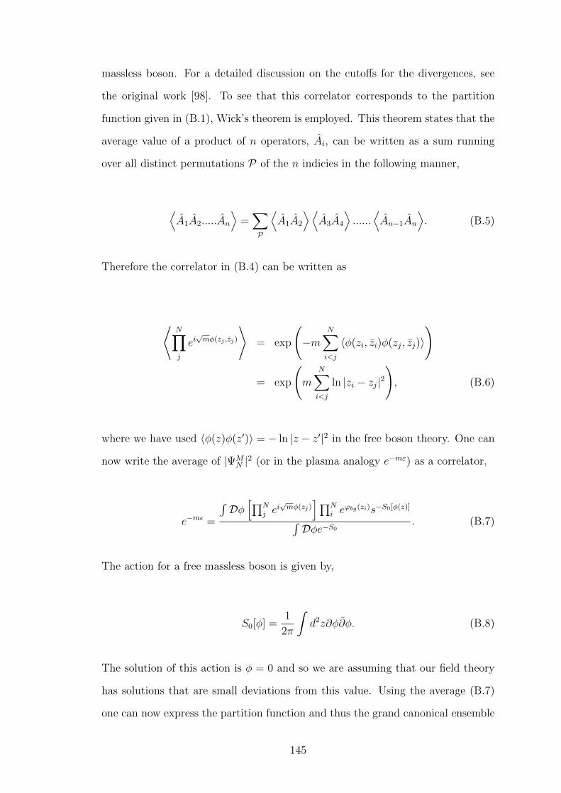
massless boson. For a detailed discussion on the cutoffs for the divergences, see
the original work [98]. To see that this correlator corresponds to the partition
function given in (B.1), Wick’s theorem is employed. This theorem states that the
average value of a product of n operators, Ai, can be written as a sum running
over all distinct permutations P of the n indicies in the following manner,
⟨A1A2.....An
⟩=∑P
⟨A1A2
⟩⟨A3A4
⟩......
⟨An−1An
⟩. (B.5)
Therefore the correlator in (B.4) can be written as
⟨N∏j
ei√mφ(zj ,zj)
⟩= exp
(−m
N∑i<j
〈φ(zi, zi)φ(zj, zj)〉
)
= exp
(m
N∑i<j
ln |zi − zj|2), (B.6)
where we have used 〈φ(z)φ(z′)〉 = − ln |z − z′|2 in the free boson theory. One can
now write the average of |ΨMN |2 (or in the plasma analogy e−mε) as a correlator,
e−mε =
∫Dφ[∏N
j ei√mφ(zj)
]∏Ni e
ϕbg(zi)s−S0[φ(z)]∫Dφe−S0
. (B.7)
The action for a free massless boson is given by,
S0[φ] =1
2π
∫d2z∂φ∂φ. (B.8)
The solution of this action is φ = 0 and so we are assuming that our field theory
has solutions that are small deviations from this value. Using the average (B.7)
one can now express the partition function and thus the grand canonical ensemble
145
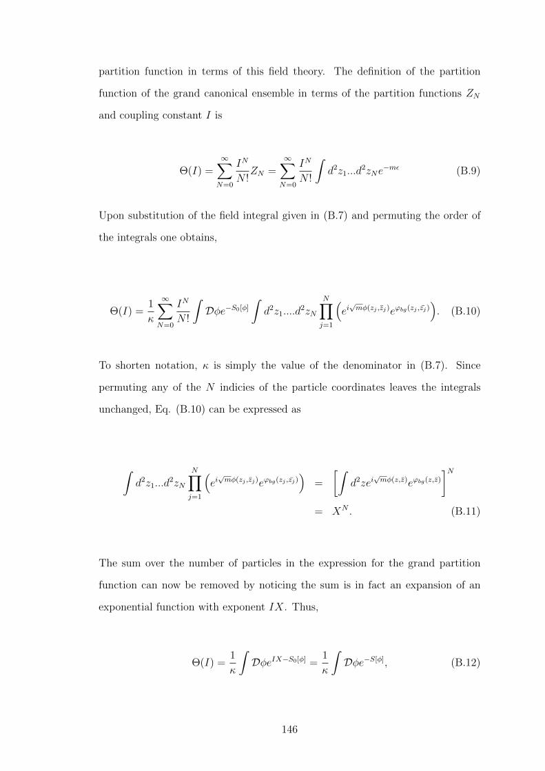
partition function in terms of this field theory. The definition of the partition
function of the grand canonical ensemble in terms of the partition functions ZN
and coupling constant I is
Θ(I) =∞∑N=0
IN
N !ZN =
∞∑N=0
IN
N !
∫d2z1...d
2zNe−mε (B.9)
Upon substitution of the field integral given in (B.7) and permuting the order of
the integrals one obtains,
Θ(I) =1
κ
∞∑N=0
IN
N !
∫Dφe−S0[φ]
∫d2z1....d
2zN
N∏j=1
(ei√mφ(zj ,zj)eϕbg(zj ,zj)
). (B.10)
To shorten notation, κ is simply the value of the denominator in (B.7). Since
permuting any of the N indicies of the particle coordinates leaves the integrals
unchanged, Eq. (B.10) can be expressed as
∫d2z1...d
2zN
N∏j=1
(ei√mφ(zj ,zj)eϕbg(zj ,zj)
)=
[∫d2zei
√mφ(z,z)eϕbg(z,z)
]N= XN . (B.11)
The sum over the number of particles in the expression for the grand partition
function can now be removed by noticing the sum is in fact an expansion of an
exponential function with exponent IX. Thus,
Θ(I) =1
κ
∫DφeIX−S0[φ] =
1
κ
∫Dφe−S[φ], (B.12)
146

where S[φ] is our new action in terms of the Bose field φ describing the ground
state FQH system depicted in Figure 1.5 and has the corresponding wavefunction
given by (1.31). The explicit form of this action is,
S[φ] =1
8π
∫d2z[(∇φ)(∇φ)− 4µei
√mφ(z,z)+ϕbg(z,z)
], (B.13)
where µ is the fugacity and is related to the coupling constant in the following
manner; µ = 2πI. Our aim is now to obtain an expression for the field φ in
terms of the complex variable z, from this expression one can calculate important
characteristics of the system such as the particle density throughout the bulk of
the FQH system.
The variational principle is employed to give the differential equation
∆ϕ(z, z) + 2mµe−ϕ(z,z) = 2− 4πMδ|z|, (B.14)
where the following change of variables has been used
φ =i√m
(ϕ+ ϕbg) . (B.15)
It is noted that the solution must be angle independent as a result of the axial
symmetry of the system and so ϕ(z, z) ≡ ϕ(r). Having the dependent variable ϕ
as the exponent of an exponential function makes (B.14) particularly difficult to
solve. However it was noticed that one can relate the term e−ϕ to the density of
particles using the two-dimensional Poisson’s equation given by
∆ϕ = 4πm(ρ− ρbg) = 4πmρ−∆ϕbg, (B.16)
147

where ρ corresponds to the charge density due to the particles creating the plasma
and ρbg is due to the neutralising background. Substituting this expression into
(B.14) gives 2mµe−ϕ = −4πmρ. Eq. (B.15) can therefore be written as a differ-
ential equation for the particle density;
1
4π∆ ln ρ+mρ = mρbg, (B.17)
where ρbg = 4πm∆ϕbg denotes background density distribution. The differential
equation (B.17) is a Liouville-type equation with an additional non-zero term on
the right-hand side. It has been discussed in Chapter 5 of this thesis. For this
section it is convenient to stick with the notation for the field ϕ(z, z) as in Eq.
(B.14). Since e−ϕ is related to density and in the semi-classical limit the bulk
density is a constant ρ = (2πml2B)−1, the differential equation for ϕ(z, z) can be
re-written as
∆ϕ(z, z)− F 2 = 2− 4πMδ|z|. (B.18)
where
F 2 =
2
ml2Bfor RI < |z| < RO,
0 otherwise.(B.19)
The solution to this differential equation is not given here since we are more in-
terested in the system that contains low energy excitations occupying the inner
and the outer boundary, as discussed in the next section. However since the low
energy excitations are treated as a perturbation to the ground state system the
differential equation (B.18) will be referred to later.
148

B.2 Laughlin States Including Edge Excitations
In the remainder of this appendix, the procedure given previously for mapping the
FQH system to a boson field theory is again used for the wavefunction given in
(3.9). Purposefully, the distance between the inner and outer boundary is greater
than the magnetic length such that the two edges do not interact with each other.
For simplicity, the wavefunction parameterised by t±k is repeated below.
Ψ =N∏i=1
(zi − zj)mN∏i=1
zMi e− |zi|
2
4+w(zi), (B.20)
where
w(z) =∑k>0
(zktk +
t−kzk
). (B.21)
This wavefunction can be expressed in terms of a partition function which will
now contain the parameters t±k.
Z(t±k, t±k) =
∫ N∏i=1
d2zie−mε(t±k,t±k) =
∫ N∏i=1
d2zi|Ψ|2, (B.22)
where the effective energy, according to (B.20) is
ε(t±k, t±k) = 2N∑i<j
ln |zi − zj|+N∑i=1
(2M
mln |zi| −
|zi|2
2m+ w(zi) + wi(z)
). (B.23)
The aim for this section is to calculate the norm of the state (B.20) in the semi-
classical limit, which is referred to as the tau-function.
149

τ(N,M, t±k, t±) = emF (N,M,t±k,t±k), (B.24)
where the function F (N,M, t±k, t±k) should have no dependence on the inverse fil-
ing factor m of the state. The problem with the partition function in (B.22) is that
the function contains an infinite sum over the t±k parameters which is difficult to
work with. Instead, the partition function Z(t±k, t±k) is mapped onto a new par-
tition function Z(a, c) using a transformation to Miwa variables [106]. Effectively,
this new partition function describes a disk-shaped quantum fluid (absent of edge
excitations) with two source charges placed at complex coordinates a and c where
a is placed in the macroscopic hole inside the disk (|a| < RI) and c is outside the
droplet (|c| > RO). This new system is described by the partition function,
Z(a, c) =
∫ N∏i=1
d2zi
N∏i<j
|zi − zj|2mN∏k=1
(eϕbg(z)k
|zi − a|2m
|zi|2m|zi − c|2m
), (B.25)
where ϕbg(z, z) = 2M ln |z| − |z|2/2, as defined in the previous section. The ex-
tra product;∏|zi|−2m has been inserted into the above partition function as a
mathematical convenience to simplify the mappings between the partition func-
tions Z(a, b) and Z(t±k, t±k). This addition reduces the number of quasiholes in
the center of the disk from M to M −m. This is not a problem as long as M > m.
To find this mapping the following expansions are used in Z(a, c);
|z − c|2m = |c|2m exp
[−m
∑k>0
(zk
kck+
zk
kck
)],
|z − a|2m = |z|2m exp
[−m
∑k>0
(ak
kzk+
ak
kzk
)].
Substituting these expansions into (B.25) and comparing Z(a, c) and Z(t±k, t±k)
150
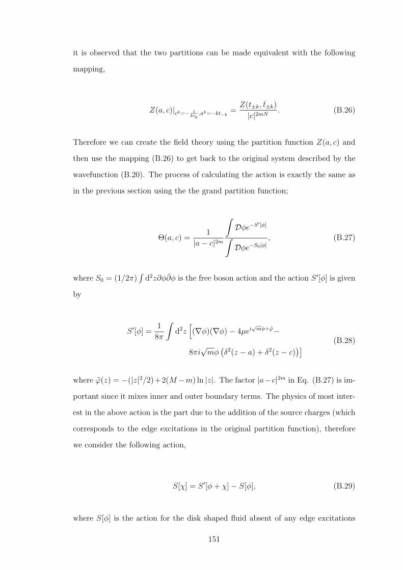
it is observed that the two partitions can be made equivalent with the following
mapping,
Z(a, c)|ck=− 1ktk
,ak=−kt−k =Z(t±k, t±k)
|c|2mN. (B.26)
Therefore we can create the field theory using the partition function Z(a, c) and
then use the mapping (B.26) to get back to the original system described by the
wavefunction (B.20). The process of calculating the action is exactly the same as
in the previous section using the the grand partition function;
Θ(a, c) =1
|a− c|2m
∫Dφe−S′[φ]∫Dφe−S0[φ]
, (B.27)
where S0 = (1/2π)∫
d2z∂φ∂φ is the free boson action and the action S ′[φ] is given
by
S ′[φ] =1
8π
∫d2z
[(∇φ)(∇φ)− 4µei
√mφ+ϕ−
8πi√mφ
(δ2(z − a) + δ2(z − c)
)] (B.28)
where ϕ(z) = −(|z|2/2)+2(M−m) ln |z|. The factor |a−c|2m in Eq. (B.27) is im-
portant since it mixes inner and outer boundary terms. The physics of most inter-
est in the above action is the part due to the addition of the source charges (which
corresponds to the edge excitations in the original partition function), therefore
we consider the following action,
S[χ] = S ′[φ+ χ]− S[φ], (B.29)
where S[φ] is the action for the disk shaped fluid absent of any edge excitations
151

and was calculated previously in Eq. (B.13). The saddle point equation for the
action S[χ] is
∆χ+ i√mF 2
(ei√mχ
R2mI
− 1
)= −4πi
√m(δ2(z − a) + δ2(z − c)
)(B.30)
where F 2 is defined in Eq. (B.19). This differential equation can be solved but
the solution, denoted χsp, is not presented here due to the expressions being long
and untidy. With the saddle point solution, the tau-function, or the norm of the
Laughlin states parameterised by t±k can be extracted via,
τ(N,M, t±k, t±) =e−S[χsp]
|a− c|2m
∣∣∣∣ck=− 1
ktk,ak=−kt−k
, (B.31)
where the mapping described in Eq. (B.26) is used to get back to the original t±k
variables. Remembering that we are only interested in the t±k and t±k dependence,
the final result following the above processes is given by
τ(N,M, t±k, t±) = D(N,M)×
exp
{m∑k>0
(kR2k
O |tk|2 + k|t−k|2
R2kI
+ kt−ktk + ktk t−k
)},
(B.32)
where D(N,M) is a function of zero mode contributions. It is noted here that
this function was also calculated using another method in [95] where the same t±k
dependence was obtained. To finalise this section, a few remarks will be made
about the types of averages performed using the field theory developed in this
appendix.
This field theory was developed using the grand canonical partition, meaning that
the states averaged over in this theory are not just energy dependent, but they
also differ in the total number of particles. It is expected that this should not
152
affect any calculations for bulk properties of the FQH fluid however, measurements
which are dependent on the boudaries of the FQH fluid may not be accurate
in this represenetation. For example consider the tau-function calculated above.
According to Eq. (B.24), the tau-function is defined for a constant number of
particles, whereas the calculation of this function using the boson field theory in
Eq. (B.31) averages over states of varying number of particles. Therefore it is
not obvious that the calculation listed here is accurate for the norm of Laughlin
states supporting edge excitations. In Chapter 3 however, this expression for the
tau-function was verified by numerically computing overlap integrals for Laughlin
states containing inner and outer boundary excitations for various cutoffs of the
orbital angular momentum.
153

Bibliography
[1] A. B. Fowler, F. F. Fang, W. E. Howard, and P. J. Stiles. Magneto-oscillatory
conductance in silicon surfaces. Phys. Rev. Lett., 16:901–903, May 1966.
[2] K. v. Klitzing, G. Dorda, and M. Pepper. New method for high-accuracy de-
termination of the fine-structure constant based on quantized Hall resistance.
Phys. Rev. Lett., 45:494–497, Aug 1980.
[3] D. C. Tsui, H. L. Stormer, and A. C. Gossard. Two-dimensional magne-
totransport in the extreme quantum limit. Phys. Rev. Lett., 48:1559–1562,
May 1982.
[4] D. C. Tsui, H. L. Stormer, J. C. M. Hwang, J. S. Brooks, and M. J. Naughton.
Observation of a fractional quantum number. Phys. Rev. B, 28:2274–2275,
Aug 1983.
[5] H. L. Stormer, A. Chang, D. C. Tsui, J. C. M. Hwang, A. C. Gossard, and
W. Wiegmann. Fractional quantization of the Hall effect. Phys. Rev. Lett.,
50:1953–1956, Jun 1983.
[6] A. M. Chang, P. Berglund, D. C. Tsui, H. L. Stormer, and J. C. M. Hwang.
Higher-order states in the multiple-series, fractional, quantum Hall effect.
Phys. Rev. Lett., 53:997–1000, Sep 1984.
[7] A. M. Chang, M. A. Paalanen, D. C. Tsui, H. L. Stormer, and J. C. M.
Hwang. Fractional quantum Hall effect at low temperatures. Phys. Rev. B,
28:6133–6136, Nov 1983.
154

[8] V. J. Goldman, M. Shayegan, and D. C. Tsui. Evidence for the fractional
quantum Hall state at ν = 17. Phys. Rev. Lett., 61:881–884, Aug 1988.
[9] P. Bonderson, A. E. Feiguin, G. Moller, and J. K. Slingerland. Competing
topological orders in the ν = 12/5 quantum Hall state. Phys. Rev. Lett.,
108:036806, Jan 2012.
[10] R. Willett, J. P. Eisenstein, H. L. Stormer, D. C. Tsui, A. C. Gossard, and
J. H. English. Observation of an even-denominator quantum number in the
fractional quantum Hall effect. Phys. Rev. Lett., 59:1776–1779, Oct 1987.
[11] W. Pan, J.-S. Xia, V. Shvarts, D. E. Adams, H. L. Stormer, D. C. Tsui,
L. N. Pfeiffer, K. W. Baldwin, and K. W. West. Exact quantization of the
even-denominator fractional quantum Hall state at ν = 5/2 Landau level
filling factor. Phys. Rev. Lett., 83:3530–3533, Oct 1999.
[12] P. L. Gammel, D. J. Bishop, J. P. Eisenstein, J. H. English, A. C. Gossard,
R. Ruel, and H. L. Stormer. Ultralow-temperature behavior of the ν = 52
fractional quantum Hall effect. Phys. Rev. B, 38:10128–10130, Nov 1988.
[13] R. B. Laughlin. Anomalous quantum Hall effect: An incompressible quantum
fluid with fractionally charged excitations. Phys. Rev. Lett., 50:1395–1398,
May 1983.
[14] E. H. Hall. On a new action of the magnet on electric currents. American
Journal of Mathematics, 2(3):pp. 287–292, 1879.
[15] T. Chakraborty and P. Pietilainen. The quantum Hall effects: integral and
fractional. Springer series in solid-state sciences. Springer-Verlag, 1995.
[16] A.H. MacDonald. Quantum Hall effect: a perspective. Perspectives in con-
densed matter physics. Kluwer Academic Publishers, 1989.
[17] Z.F. Ezawa. Quantum Hall Effects: Field Theoretical Approach and Related
Topics. World Scientific, 2008.
155

[18] N.W. Ashcroft and N.D. Mermin. Solid State Physics. Cengage Learning,
2011.
[19] L. D. Landau and E. M. Lifshitz. Quantum mechanics: non-relativistic
theory. Oxford; Boston: Butterworth-Heinemann, 3rd ed., rev. and enl., repr.
1991 with corrections edition, 1991. Translation of: Kvantovaia mekhanika.
[20] R. B. Laughlin. Quantized Hall conductivity in two dimensions. Phys. Rev.
B, 23:5632–5633, May 1981.
[21] B. I. Halperin. Quantized Hall conductance, current-carrying edge states,
and the existence of extended states in a two-dimensional disordered poten-
tial. Phys. Rev. B, 25:2185–2190, Feb 1982.
[22] Qian Niu and D. J. Thouless. Quantum Hall effect with realistic boundary
conditions. Phys. Rev. B, 35:2188–2197, Feb 1987.
[23] Richard E Prange and Steven M Girvin. The Quantum Hall effect. New
York: Springer-Verlag, 2nd ed edition, 1990.
[24] F. D. M. Haldane. Fractional quantization of the Hall effect: A hierarchy
of incompressible quantum fluid states. Phys. Rev. Lett., 51:605–608, Aug
1983.
[25] J.M. Caillol, D. Levesque, J.J. Weis, and J.P. Hansen. A monte carlo study of
the classical two-dimensional one-component plasma. Journal of Statistical
Physics, 28(2):325–349, 1982.
[26] W. J. He, T. Cui, Y. M. Ma, C. B. Chen, Z. M. Liu, and G. T. Zou. Phase
boundary between the fractional quantum Hall liquid and the Wigner crystal
at low filling factors and low temperatures: A path integral monte carlo
study. Phys. Rev. B, 72:195306, Nov 2005.
[27] Daniel Arovas, J. R. Schrieffer, and Frank Wilczek. Fractional statistics and
the quantum Hall effect. Phys. Rev. Lett., 53:722–723, Aug 1984.
156

[28] F. E. Camino, Wei Zhou, and V. J. Goldman. Realization of a Laughlin
quasiparticle interferometer: Observation of fractional statistics. Phys. Rev.
B, 72:075342, Aug 2005.
[29] F. E. Camino, Wei Zhou, and V. J. Goldman. e/3 Laughlin quasiparticle
primary-filling ν= 1/3 interferometer. Phys. Rev. Lett., 98:076805, Feb 2007.
[30] M. Oshikawa, Y. B. Kim, K. Shtengel, C. Nayak, and S. Tewari. Topo-
logical degeneracy of non-Abelian states for dummies. Annals of Physics,
322(6):1477 – 1498, 2007.
[31] C. Nayak, S. H. Simon, A. Stern, M. Freedman, and S. Das Sarma. Non-
Abelian anyons and topological quantum computation. Rev. Mod. Phys.,
80:1083–1159, Sep 2008.
[32] N. E. Bonesteel, L. Hormozi, G. Zikos, and S. H. Simon. Quantum computing
with non-Abelian quasiparticles. International Journal of Modern Physics
B, 21(08n09):1372–1378, 2007.
[33] P. Bonderson, M. Freedman, and C. Nayak. Measurement-only topological
quantum computation. Phys. Rev. Lett., 101:010501, Jun 2008.
[34] L. Hormozi, N. E. Bonesteel, and S. H. Simon. Topological quantum com-
puting with Read-Rezayi states. Phys. Rev. Lett., 103:160501, Oct 2009.
[35] S. Das Sarma, M. Freedman, and C. Nayak. Topologically protected qubits
from a possible non-Abelian fractional quantum Hall state. Phys. Rev. Lett.,
94:166802, Apr 2005.
[36] G. Moore and N. Read. Nonabelions in the fractional quantum Hall effect.
Nuclear Physics B, 360(23):362 – 396, 1991.
[37] E. Fradkin, C. Nayak, A. Tsvelik, and F. Wilczek. A Chern-Simons effec-
tive field theory for the Pfaffian quantum Hall state. Nuclear Physics B,
516(3):704 – 718, 1998.
157
[38] N. Read and E. Rezayi. Beyond paired quantum Hall states: Parafermions
and incompressible states in the first excited Landau level. Phys. Rev. B,
59:8084–8092, Mar 1999.
[39] N. Read and E. Rezayi. Quasiholes and fermionic zero modes of paired
fractional quantum Hall states: The mechanism for non-Abelian statistics.
Phys. Rev. B, 54:16864–16887, Dec 1996.
[40] P. Bonderson, A. Kitaev, and K. Shtengel. Detecting non-Abelian statistics
in the ν = 5/2 fractional quantum Hall state. Phys. Rev. Lett., 96:016803,
Jan 2006.
[41] R. L. Willett, L. N. Pfeiffer, and K. W. West. Alternation and interchange
of e/4 and e/2 period interference oscillations consistent with filling factor
5/2 non-Abelian quasiparticles. Phys. Rev. B, 82:205301, Nov 2010.
[42] X. Lin, C. Dillard, M. A. Kastner, L. N. Pfeiffer, and K. W. West. Measure-
ments of quasiparticle tunneling in the υ = 52
fractional quantum Hall state.
Phys. Rev. B, 85:165321, Apr 2012.
[43] Guang Yang and D. E. Feldman. Influence of device geometry on tunneling
in the ν = 52
quantum Hall liquid. Phys. Rev. B, 88:085317, Aug 2013.
[44] Guang Yang and D. E. Feldman. Experimental constraints and a possible
quantum Hall state at ν = 5/2. Phys. Rev. B, 90:161306, Oct 2014.
[45] V. Cheianov S. J. Huntington. Zero mode tunnelling in a fractional quantum
Hall device. To be published, 2015.
[46] X. G. Wen. Chiral Luttinger liquid and the edge excitations in the fractional
quantum Hall states. Phys. Rev. B, 41, 1990.
[47] C. W. J. Beenakker. Edge channels for the fractional quantum Hall effect.
Phys. Rev. Lett., 64:216–219, Jan 1990.
158

[48] C. L. Kane and Matthew P. A. Fisher. Transmission through barriers and
resonant tunneling in an interacting one-dimensional electron gas. Physical
Review B, 46(23):15233, 1992.
[49] C. L. Kane and Matthew P. A. Fisher. Resonant tunneling in an interacting
one-dimensional electron gas. Phys. Rev. B, 46:7268–7271, Sep 1992.
[50] C. L. Kane and Matthew P. A. Fisher. Transport in a one-channel Luttinger
liquid. Phys. Rev. Lett., 68:1220–1223, Feb 1992.
[51] A. Furusaki and N. Nagaosa. Single-barrier problem and Anderson localiza-
tion in a one-dimensional interacting electron system. Phys. Rev. B, 47:4631–
4643, Feb 1993.
[52] K. Moon, H. Yi, C. L. Kane, S. M. Girvin, and Matthew P. A. Fisher.
Resonant tunneling between quantum Hall edge states. Phys. Rev. Lett.,
71:4381–4384, Dec 1993.
[53] A.O. Gogolin, A.A. Nersesyan, and A.M. Tsvelik. Bosonization and Strongly
Correlated Systems. Cambridge University Press, 2004.
[54] F.P. Milliken, C.P. Umbach, and R.A. Webb. Indications of a Luttinger
liquid in the fractional quantum Hall regime. Solid State Communications,
97(4):309 – 313, 1996.
[55] S. Roddaro, V. Pellegrini, F. Beltram, G. Biasiol, and L. Sorba. Interedge
strong-to-weak scattering evolution at a constriction in the fractional quan-
tum Hall regime. Phys. Rev. Lett., 93:046801, Jul 2004.
[56] A. M. Chang, L. N. Pfeiffer, and K. W. West. Observation of chiral Luttinger
behavior in electron tunneling into fractional quantum Hall edges. Phys. Rev.
Lett., 77:2538–2541, Sep 1996.
[57] C. L. Kane and Matthew P. A. Fisher. Nonequilibrium noise and fractional
charge in the quantum Hall effect. Phys. Rev. Lett., 72:724–727, Jan 1994.
159

[58] L. Saminadayar, D. C. Glattli, Y. Jin, and B. Etienne. Observation of the e/3
fractionally charged Laughlin quasiparticle. Phys. Rev. Lett., 79:2526–2529,
Sep 1997.
[59] R. dePicciotto, M. Reznikov, M. Heiblum, V. Umansky, G. Bunin, and
D. Mahalu. Direct observation of a fractional charge. Nature, 389(6647):162–
164, SEP 11 1997.
[60] M. Dolev, Y. Gross, Y. C. Chung, M. Heiblum, V. Umansky, and D. Ma-
halu. Dependence of the tunneling quasiparticle charge determined via shot
noise measurements on the tunneling barrier and energetics. Phys. Rev. B,
81:161303, Apr 2010.
[61] S. Baer, C. Rossler, T. Ihn, K. Ensslin, C. Reichl, and W. Wegscheider.
Experimental probe of topological orders and edge excitations in the second
Landau level. Phys. Rev. B, 90:075403, Aug 2014.
[62] P. Fendley, A. W. W. Ludwig, and H. Saleur. Exact conductance through
point contacts in the ν = 1/3 fractional quantum Hall effect. Phys. Rev.
Lett., 74:3005–3008, Apr 1995.
[63] R. Guyon, P. Devillard, T. Martin, and I. Safi. Klein factors in multiple
fractional quantum Hall edge tunneling. Phys. Rev. B, 65:153304, Mar 2002.
[64] C. L. Kane. Telegraph noise and fractional statistics in the quantum Hall
effect. Phys. Rev. Lett., 90:226802, Jun 2003.
[65] I. Safi, P. Devillard, and T. Martin. Partition noise and statistics in the
fractional quantum Hall effect. Phys. Rev. Lett., 86:4628–4631, May 2001.
[66] K. T. Law, D. E. Feldman, and Yuval Gefen. Electronic mach-zehnder inter-
ferometer as a tool to probe fractional statistics. Phys. Rev. B, 74:045319,
Jul 2006.
160

[67] S. Vishveshwara. Revisiting the Hanbury Brown-Twiss setup for fractional
statistics. Phys. Rev. Lett., 91:196803, Nov 2003.
[68] C. Nayak, Matthew P. A. Fisher, A. W. W. Ludwig, and H. H. Lin. Resonant
multilead point-contact tunneling. Phys. Rev. B, 59:15694–15704, Jun 1999.
[69] V. V. Ponomarenko and D. V. Averin. Strong-coupling branching between
edges of fractional quantum Hall liquids. Phys. Rev. B, 70:195316, Nov 2004.
[70] T. Jonckheere, P. Devillard, A. Crepieux, and T. Martin. Electronic mach-
zehnder interferometer in the fractional quantum Hall effect. Phys. Rev. B,
72:201305, Nov 2005.
[71] N. Datta, R. Morf, and R. Ferrari. Edge of the Laughlin droplet. Phys. Rev.
B, 53:10906–10915, Apr 1996.
[72] T. Can, P. J. Forrester, G. Tellez, and P. Wiegmann. Singular behavior at
the edge of Laughlin states. Phys. Rev. B, 89:235137, Jun 2014.
[73] R. C. Gann, Sudip Chakravarty, and G. V. Chester. Monte carlo simula-
tion of the classical two-dimensional one-component plasma. Phys. Rev. B,
20:326–344, Jul 1979.
[74] D. Ceperley. Ground state of the fermion one-component plasma: A monte
carlo study in two and three dimensions. Phys. Rev. B, 18:3126–3138, Oct
1978.
[75] J. P. Hansen. Statistical mechanics of dense ionized matter. i. equilibrium
properties of the classical one-component plasma. Phys. Rev. A, 8:3096–3109,
Dec 1973.
[76] J.M. Caillol, D. Levesque, J.J. Weis, and J.P. Hansen. A monte carlo study of
the classical two-dimensional one-component plasma. Journal of Statistical
Physics, 28(2):325–349, 1982.
161

[77] D. Levesque, J. J. Weis, and A. H. MacDonald. Crystallization of the incom-
pressible quantum-fluid state of a two-dimensional electron gas in a strong
magnetic field. Phys. Rev. B, 30:1056–1058, Jul 1984.
[78] R. Morf and B. I. Halperin. Monte carlo evaluation of trial wave functions for
the fractional quantized Hall effect: Disk geometry. Phys. Rev. B, 33:2221–
2246, Feb 1986.
[79] M. E. J. Newman and G. T. Barkema. Monte Carlo Methods in Statistical
Physics. Oxford University Press, 1999.
[80] W. L. McMillan. Ground state of liquid He4. Phys. Rev., 138:A442–A451,
Apr 1965.
[81] N. Metropolis, A. W. Rosenbluth, M. N. Rosenbluth, A. H. Teller, and
E. Teller. Equation of state calculations by fast computing machines. The
Journal of Chemical Physics, 21(6):1087–1092, 1953.
[82] H. Mller-Krumbhaar and K. Binder. Dynamic properties of the monte carlo
method in statistical mechanics. Journal of Statistical Physics, 8(1):1–24,
1973.
[83] K. Binder, K. Binder, D.M. Ceperley, J.P. Hansen, H. Kalos, D.P. Landau,
D. Levesque, H. Muller-Krumbhaar, D. Stauffer, and J.J. Weis. Monte Carlo
Methods in Statistical Physics. Topics in Current Physics. Springer Berlin
Heidelberg, 1986.
[84] FDM Haldane. Edge states and boundary fluctuations in the quantum Hall
fluid. Bull. Am. Phys. Soc, 35:254, 1990.
[85] S. A. Trugman and S. Kivelson. Exact results for the fractional quantum
Hall effect with general interactions. Phys. Rev. B, 31:5280–5284, Apr 1985.
[86] X.G. Wen. Theory of the edge states in fractional quantum Hall effects.
International Journal of Modern Physics B, 06(10):1711–1762, 1992.
162
[87] M. Stone. Schur functions, chiral bosons, and the quantum-Hall-effect edge
states. Phys. Rev. B, 42:8399–8404, Nov 1990.
[88] J. M. Luttinger. An exactly soluble model of a manyfermion system. Journal
of Mathematical Physics, 4(9):1154–1162, 1963.
[89] S. Tomonaga. Remarks on bloch’s method of sound waves applied to many-
fermion problems. Progress of Theoretical Physics, 5(4):544–569, 1950.
[90] D. C. Mattis and E. H. Lieb. Exact solution of a manyfermion system and
its associated boson field. Journal of Mathematical Physics, 6(2):304–312,
1965.
[91] A. Luther and I. Peschel. Single-particle states, kohn anomaly, and pairing
fluctuations in one dimension. Phys. Rev. B, 9:2911–2919, Apr 1974.
[92] F. D. M. Haldane. ‘Luttinger liquid theory’ of one-dimensional quantum
fluids. i. properties of the Luttinger model and their extension to the general
1d interacting spinless fermi gas. Journal of Physics C: Solid State Physics,
14(19):2585, 1981.
[93] A. M. Chang. Chiral Luttinger liquids at the fractional quantum Hall edge.
Rev. Mod. Phys., 75:1449–1505, Nov 2003.
[94] A. Boyarsky, V. V. Cheianov, and O. Ruchayskiy. Microscopic construction
of the chiral Luttinger liquid theory of the quantum Hall edge. Phys. Rev.
B, 70:235309, Dec 2004.
[95] E. V. Sukhorukov I. P. Levkivskyi, J. Froehlich. Topological screening and
interference of fractionally charged quasi-particles. arXiv:1005.5703v1 [cond-
mat.mes-hall], 2010.
[96] I. K. Kostov, I. Krichever, M. Mineev-Weinstein, P. Wiegmann, and
A. Zabrodin. Tau-function for analytic curves. Random matrices and their
applications, MSRI (eprint arXiv:hep-th/0005259), 40:285, may 2000.
163

[97] P. Wiegmann and A. Zabrodin. Large N expansion for normal and complex
matrix ensembles. In Frontiers in Number Theory, Physics, and Geometry
I, pages 213–229. Springer, 2006.
[98] A. Boyarsky, V. V. Cheianov, and O. Ruchayskiy. Fermions in the harmonic
potential and string theory. Journal of High Energy Physics, 2005(01):010,
2005.
[99] P. Wiegmann and A. Zabrodin. Large scale correlations in normal non-
Hermitian matrix ensembles. Journal of Physics A: Mathematical and Gen-
eral, 36(12):3411, 2003.
[100] A. Zabrodin. New applications of non-Hermitian random matrices. Annales
Henri Poincar, 4(2):851–861, 2003.
[101] A. Zabrodin and P. Wiegmann. Large-N expansion for the 2d dyson gas.
Journal of Physics A: Mathematical and General, 39(28):8933, 2006.
[102] P. Bonderson, V. Gurarie, and C. Nayak. Plasma analogy and non-Abelian
statistics for Ising-type quantum Hall states. Phys. Rev. B, 83:075303, Feb
2011.
[103] D.E. Littlewood. A University Algebra. Heinemann, 1958.
[104] I. G. Macdonald. Symmetric Functions and Hall Polynomials. Oxford math-
ematical monographs. Clarendon Press, 1998.
[105] M. Stone, H. W. Wyld, and R. L. Schult. Edge waves in the quantum Hall
effect and quantum dots. Phys. Rev. B, 45:14156–14161, Jun 1992.
[106] B. Konopelchenko and L. M. Alonso. The KP hierarchy in Miwa coordinates.
Physics Letters A, 258(46):272 – 278, 1999.
164