microsoft excel 2007 beginning - osceola school …... then programs>microsoft...

March 2012 Rev.2 BLFM Pg 1 officebeginningexcel.docx

Microsoft Excel 2007 – Beginning The information below is devoted to Microsoft Excel and the basics of the program.

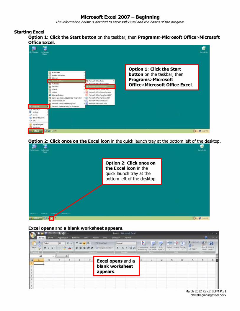
Starting Excel

Option 1: Click the Start button on the taskbar, then Programs>Microsoft Office>Microsoft Office Excel.

Option 2: Click once on the Excel icon in the quick launch tray at the bottom left of the desktop.

Excel opens and a blank worksheet appears.

Option 1: Click the Start button on the taskbar, then Programs>Microsoft Office>Microsoft Office Excel.

Option 2: Click once on the Excel icon in the quick launch tray at the

bottom left of the desktop.

Excel opens and a blank worksheet

appears.


Worksheet window The worksheet window contains a grid of columns and rows.

The columns are labeled alphabetically (A, B C, etc.) and the rows are labeled numerically (1, 2, 3, etc.). The worksheet window displays only a tiny piece of the whole worksheet available (there are 256 columns and 65,536 rows available).

The intersection of a column and row is called a cell. Cells can contain text, numbers, formulas, or a combination of all three. Every cell has its own unique location or cell address identified by the coordinates of the intersecting column and row. For example: B3 is the cell in the 2nd column (B), third row (3).

The worksheet window contains a grid of columns and rows.

The columns are labeled alphabetically (A, B C, etc.) and the rows are labeled numerically (1, 2, 3, etc.).

The intersection of a column and row is called a cell. Cells can contain text, numbers, formulas, or a combination of all three. Every cell has its own unique location or cell address identified by the coordinates of the intersecting column and row. For example: B3 is the

cell in the 2nd column (B), third row (3).


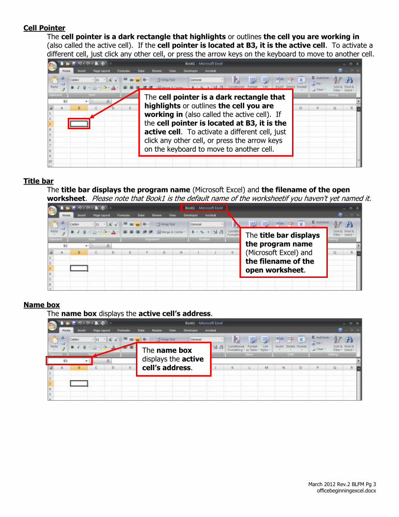
Cell Pointer The cell pointer is a dark rectangle that highlights or outlines the cell you are working in (also called the active cell). If the cell pointer is located at B3, it is the active cell. To activate a different cell, just click any other cell, or press the arrow keys on the keyboard to move to another cell.

Title bar The title bar displays the program name (Microsoft Excel) and the filename of the open worksheet. Please note that Book1 is the default name of the worksheetif you haven't yet named it.

Name box The name box displays the active cell’s address.

The cell pointer is a dark rectangle that highlights or outlines the cell you are working in (also called the active cell). If the cell pointer is located at B3, it is the active cell. To activate a different cell, just click any other cell, or press the arrow keys on the keyboard to move to another cell.

The title bar displays the program name (Microsoft Excel) and the filename of the

open worksheet.

The name box displays the active cell’s address.


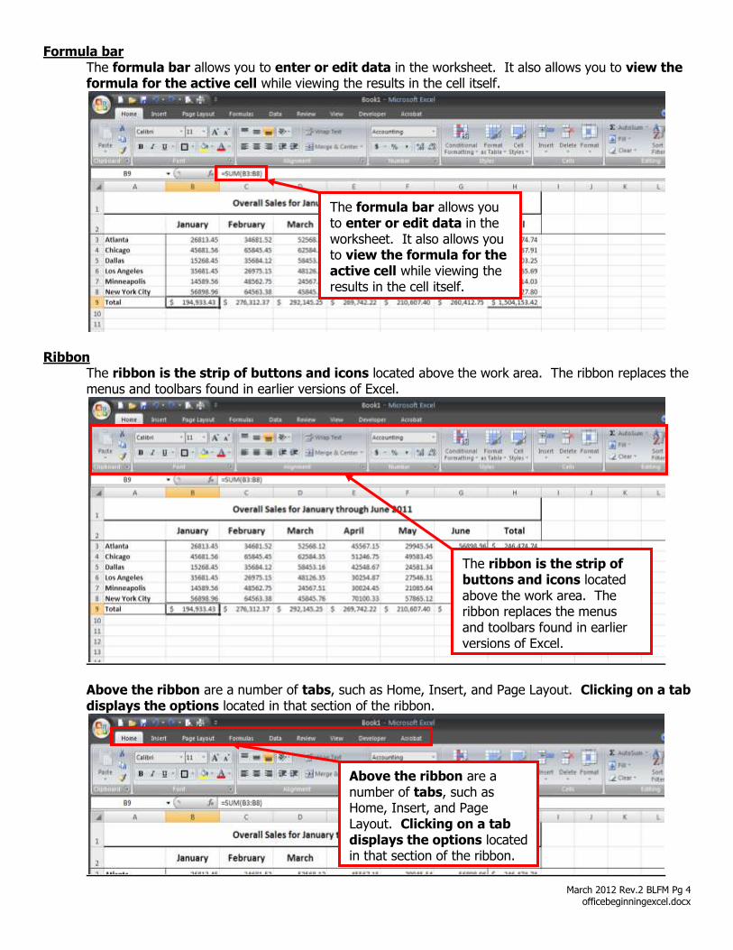
Formula bar The formula bar allows you to enter or edit data in the worksheet. It also allows you to view the formula for the active cell while viewing the results in the cell itself.

Ribbon

The ribbon is the strip of buttons and icons located above the work area. The ribbon replaces the menus and toolbars found in earlier versions of Excel.

Above the ribbon are a number of tabs, such as Home, Insert, and Page Layout. Clicking on a tab displays the options located in that section of the ribbon.

The formula bar allows you to enter or edit data in the worksheet. It also allows you to view the formula for the active cell while viewing the results in the cell itself.

The ribbon is the strip of buttons and icons located above the work area. The ribbon replaces the menus and toolbars found in earlier versions of Excel.

Above the ribbon are a number of tabs, such as Home, Insert, and Page Layout. Clicking on a tab displays the options located in that section of the ribbon.


Sheet Tabs The sheet tabs are located below the worksheet grid.

To rename a sheet, right-click the current name and then click Rename.

Give your sheet a new name and hit the enter button on your keyboard.

The sheet tabs are located below the worksheet grid.

To rename a sheet, right-click the current name and then click Rename.

Give your sheet a new name and hit the enter button on your keyboard.


Entering Data into a Cell 1) Type January in cell B2.

2) Press the enter button on your keyboard. What happens? It automatically “finalizes” what

you’ve typed and moves to the next cell just below the cell you entered the data into.

3) Type February in cell B3.

4) Press the Tab button on your keyboard. What happens? It automatically “finalizes” what you’ve

typed and moves to the next cell just to the right of the cell you entered the data into. Please note that you can also use the arrow buttons on the keyboard to move to a different cell.

AutoComplete When you type a word or phrase into a cell and you want to type the same word within that same column, Excel can “AutoComplete” what you want entered. For example, if you type the word Osceola into the cell B3 and then you want it in cell B4 also, will will need to start typing “Osc” into B4. Excel starts filling in the rest of the word for you. To have it complete the word, hit the enter button or the tab button on your keyboard to accept the word. Please note that if you do not want the word or phrase that Excel is trying to complete for you, keep typing to enter a different word.

Press the enter button on your keyboard. What happens? It automatically “finalizes” what you’ve typed and moves to the next cell just below the cell you entered the data into.

Type January in cell B2.

Press the Tab button on your keyboard. What happens? It automatically “finalizes” what you’ve typed and moves to the next cell just to the right of the cell you entered the data into.

Type February in cell B3.

When you type a word or phrase into a cell and you want to type the same word within that same column, Excel can “AutoComplete” what you want entered. For example, if you type the word Osceola into the cell B3 and then you want it in cell B4 also, will will need to start typing “Osc” into B4. Excel starts filling in the rest of the word for you. To have it complete the word, hit the enter button or the tab button on your keyboard to accept the word.


AutoFill 1) Go to cell B3. While the cell is “active” (it has the bold border around the cell), place your

mouse at the bottom right corner of the cell until it shows a solid black “+” as your arrow. This is called the “fill handle.”

2) Click and drag the fill handle down several cells.

3) AutoFill automatically filled in the rest of the series of months. Please note that you can also do this in rows or with days of the week, numbers, letters of the alphabet, etc.

Go to cell B3. While the cell is “active” (it has the bold border around the cell), place your mouse at the bottom right corner of the cell until it shows a solid black “+” as your arrow. This is called the “fill handle.”

Click and drag the fill handle down several cells.

AutoFill automatically filled in the rest of the series of months.


Changing column widths To change the column widths, put your mouse between the column letters. When your mouse changes to a + with arrows pointing left and right, click and drag the + to make the column wider or narrower.

Changing row height To change the row height, put your mouse between the row numbers. When your mouse changes to a + with arrows pointing up and down, click and pull the + to make the row taller or shorter.

Insert a Row

Option 1: Select a row by clicking on its number in the row header. Then on the Home tab, in the Cells group, click the arrow below Insert. Then click Insert Sheet Rows.

To change the column widths, put your mouse between the column letters. When your mouse changes to a + with arrows pointing left and right, click and drag the + to make the column wider or narrower.

To change the row height, put your mouse between the row numbers. When your mouse changes to a + with arrows pointing up and down, click and pull the + to make the row taller or shorter.

Select a row by clicking on its number in the row header. Then on the Home tab, in the Cells group, click the arrow below Insert.

Then click Insert Sheet Rows.


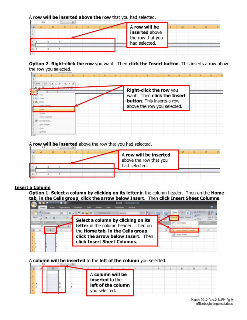
A row will be inserted above the row that you had selected.

Option 2: Right-click the row you want. Then click the Insert button. This inserts a row above the row you selected.


Insert a Column Option 1: Select a column by clicking on its letter in the column header. Then on the Home tab, in the Cells group, click the arrow below Insert. Then click Insert Sheet Columns.

A column will be inserted to the left of the column you selected.

Right-click the row you want. Then click the Insert button. This inserts a row above the row you selected.

Select a column by clicking on its letter in the column header. Then on the Home tab, in the Cells group, click the arrow below Insert. Then click Insert Sheet Columns.



A column will be inserted to the left of the column

you selected.


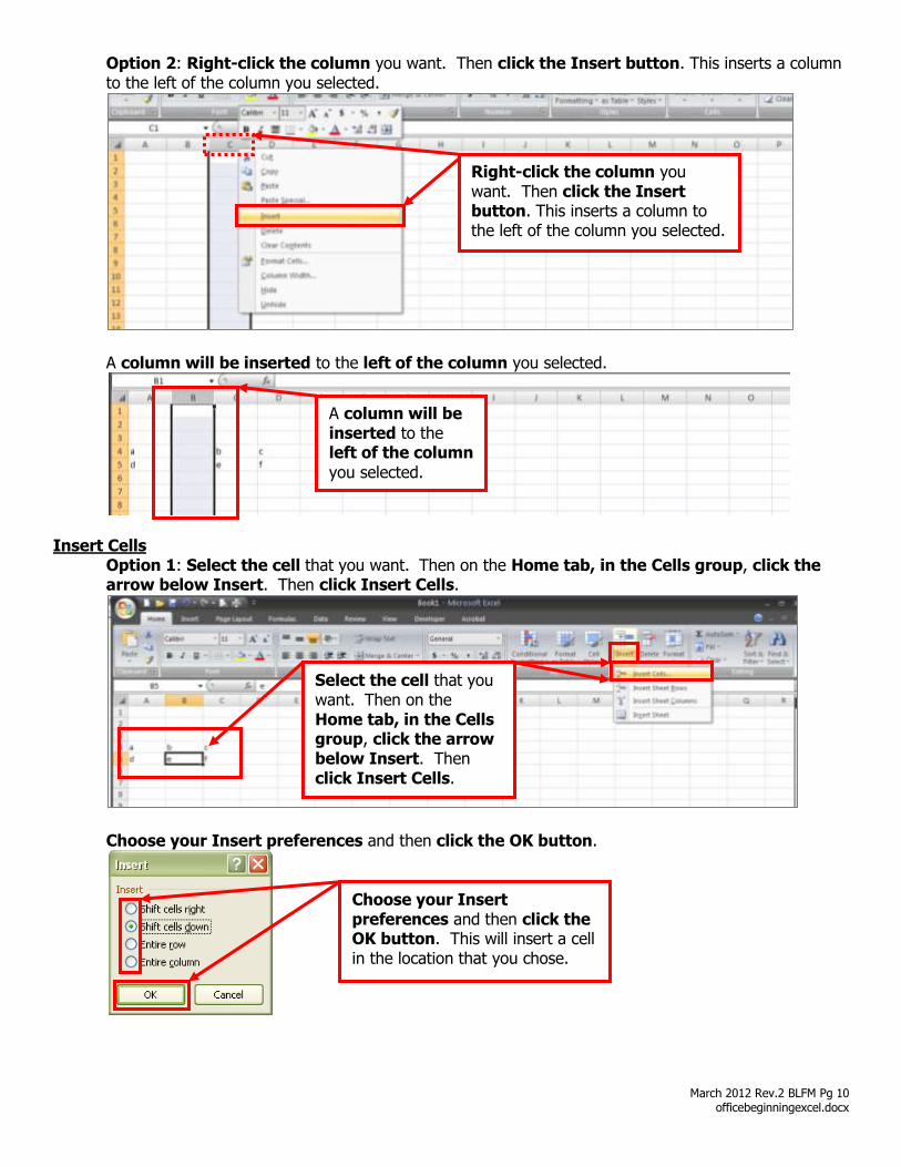
Option 2: Right-click the column you want. Then click the Insert button. This inserts a column to the left of the column you selected.

A column will be inserted to the left of the column you selected.

Insert Cells Option 1: Select the cell that you want. Then on the Home tab, in the Cells group, click the arrow below Insert. Then click Insert Cells.

Choose your Insert preferences and then click the OK button.

Right-click the column you want. Then click the Insert button. This inserts a column to the left of the column you selected.

Select the cell that you want. Then on the Home tab, in the Cells group, click the arrow below Insert. Then click Insert Cells.

Choose your Insert preferences and then click the OK button. This will insert a cell in the location that you chose.

A column will be inserted to the left of the column

you selected.


A cell will be inserted in the location that you chose.

Option 2: Right-click the cell that you want. Then click the Insert button.



Right-click the cell that you want. Then click the Insert button.



A cell will be inserted in

the location that you chose.


Delete a row or column Option 1: Select a column or row that you want to delete by clicking on its letter or number in the column/row header. Then on the Home tab, in the Cells group, click the arrow below Delete. Then click Delete Sheet Columns.

The column you selected is then deleted.

Option 2: Right-click the column you want to delete. Then click the Delete button.


Select a column or row that you want to delete by clicking on its letter or number in the column/row header. Then on the Home tab, in the Cells group, click the arrow below Delete. Then click Delete Sheet Columns.

Right-click the column you want to delete. Then click the Delete button.




Adding borders It is common to put a border under a row of labels to make your spreadsheet easier to read. To add a border, click the cell(s) you want to have a border around. Then click the arrow next to the border icon located on the Home tab, in the Font group.

Click on the type of border you would like applied to the cell(s) you have selected.

A border is then applied to the cell(s) you had selected. Please note that you might have to click out of the cell(s) before you can see the changes that have been made.

It is common to put a border under a row of labels to make your spreadsheet easier to read. To add a border, click the cell(s) you want to have a border around. Then click the arrow next to the border icon located on the Home tab, in the Font group.

Click on the type of border you would like applied to the cell(s) you have selected.

A border is then applied to the cell(s)

you had selected.


Formulas Click the cell where you want the “answer” or total to be located and type an = sign in the cell.

Type in the formula that you want excel to perform. For this example, we are going to add up cells B3 through B8. Type the word “SUM” and then (B3:B8). Then hit the enter button on the keyboard. Please note that you can add the cells individually or do other formulas.

The cell now contains the answer to the formula you typed in. Please note that you can view your formula by clicking on the cell that contains the answer – you are able to view the “formula” by looking in the formula bar.

Editing Data To delete existing data, select a cell and press the delete button on the keyboard. Please note that you can also go to the formula bar and backspace over existing data. You can edit data by clicking inside the cell and then typing your new data. You can move data by using cut and paste. Select the cell(s) you want to move and then click the Copy icon, located on the Home tab, in the Clipboard section. Then click the cell for the new location for the cell(s), and click the Paste icon, located on the Home tab, in the Clipboard section.

Click the cell where you want the “answer” or total to be located and type an = sign in the cell.

Type in the formula that you want excel to perform. For this example, we are going to add up cells B3 through B8. Type the word “SUM” and then (B3:B8). Then hit the enter button on the keyboard.

The cell now contains the answer to the formula you typed in.

microsoft excel 2007 beginning - osceola school …... then programs>microsoft...

Documents