Microstructures to Control Elasticity in 3D Printing

Christian Schumacher1,2 Bernd Bickel1,3 Jan Rys2 Steve Marschner4 Chiara Daraio2 Markus Gross1,2

1Disney Research Zurich 2ETH Zurich 3IST Austria 4Cornell University

Figure 1: Given a virtual object with specified elasticity material parameters (blue=soft, red=stiff), our method computes an assemblage ofsmall-scale structures that approximates the desired elastic behavior and requires only a single material for fabrication.

Abstract

We propose a method for fabricating deformable objects with spa-tially varying elasticity using 3D printing. Using a single, relativelystiff printer material, our method designs an assembly of small-scale microstructures that have the effect of a softer material at theobject scale, with properties depending on the microstructure usedin each part of the object. We build on work in the area of meta-materials, using numerical optimization to design tiled microstruc-tures with desired properties, but with the key difference that ourmethod designs families of related structures that can be interpo-lated to smoothly vary the material properties over a wide range.To create an object with spatially varying elastic properties, we tilethe object’s interior with microstructures drawn from these families,generating a different microstructure for each cell using an efficientalgorithm to select compatible structures for neighboring cells. Weshow results computed for both 2D and 3D objects, validating sev-eral 2D and 3D printed structures using standard material tests aswell as demonstrating various example applications.

CR Categories: I.3.5 [Computer Graphics]: Computational Ge-ometry and Object Modeling—Physically based modeling

Keywords: fabrication, topology optimization, 3D printing

1 Introduction

With the emergence of affordable 3D printing hardware and on-line 3D printing services, additive manufacturing technology comeswith the promise to make the creation of complex functional phys-ical artifacts as easy as providing a virtual description. Many func-tional objects in our everyday life consist of elastic, deformable

material, and the material properties are often inextricably linked tofunction. Unfortunately, elastic properties are not as easy to controlas geometry, since additive manufacturing technologies can usuallyuse only a single material, or a very small set of materials, whichoften do not match the desired elastic deformation behavior. How-ever, 3D printing easily creates complex, high-resolution 3D struc-tures, enabling the creation of metamaterials with properties thatare otherwise unachievable with available printer materials.

Metamaterials are assemblies of small-scale structures that obtaintheir bulk properties from the shape and arrangement of the struc-tures rather than from the composition of the material itself. Forexample, based on this principle, Lakes [1987] presented the firstengineered materials that exhibit a negative Poisson’s ratio. Sincethen, numerous designs have been proposed, usually consisting ofa periodic tiling of a basic pattern, and engineering their structuresis an active area of research [Lee et al. 2012].

While designing a tiled microstructure to match given homoge-neous material properties can be achieved with modest extensionsto the state of the art, designing a complex microstructural assem-bly to achieve heterogeneous, spatially varying properties is muchmore challenging. We face a complex inverse problem: to deter-mine a discrete small-scale material distribution at the resolutionof the 3D printer that yields the desired macroscopic elastic behav-ior. Inverse problems of this type have been explored for designingperiodic structures that can be tiled to synthesize homogeneous vol-umes, but the methods are computation-intensive and do not scaleto designing non-periodic structures for objects with spatially vary-ing material properties.

Our goal is to enable users to employ metamaterials in their 3Dprinting workflow, generating appropriate structures specifically fortheir available 3D printer model and base material within seconds.Clearly, designing entire models on the fly by directly optimiz-ing over the whole structure is impractical. Instead, we propose adata-driven approach that efficiently assembles models out of pre-computed small-scale structures so that the result both resemblesthe desired local elasticity and also is within the capabilities of theavailable output device.

First, we precompute a database of tiled structures indexed by theirelastic properties. We want these structures to cover a large andideally continuous region in the space of possible elastic behaviors.To achieve this goal, we introduce an optimization method for sam-pling structures that exhibit a range of desired behaviors, but are

also sufficiently similar to allow interpolation. We initialize thisoptimization method either with a known structure or desired elas-tic property values, and then compute a family of similar structuresthat covers a subspace of possible elastic behaviors. We repeat thisprocess, each time adding a new family of structures, to increasethe coverage of the material space.

Second, to synthesize the metamaterials for a specific object, we tilethe object’s interior with microstructures drawn from these families.Note that the same elastic behavior can be reproduced by structuresthat differ significantly in shape, and therefore the families mightoverlap in material space. This is an important feature of our sys-tem for reproducing spatially varying material behavior. Spatiallyneighboring structures must connect properly at their interface, andoverlapping families provide us with a set of candidates for eachtile, significantly increasing the chance of finding structures com-patible with neighboring tiles. We propose an efficient global opti-mization algorithm that selects an optimized tiling, taking into ac-count the need for neighboring structures to connect properly. Ourfinal result is functional and 3D printable.

We evaluate our algorithm by fabricating several examples of bothflat sheets and 3D objects with heterogeneous material behavior.For several isotropic and anisotropic 2D examples and isotropic 3Dexamples, we measure the resulting elastic properties, comparingthe actual material parameters to the values predicted by our simu-lation.

2 Related Work

Simulation and Homogenization Simulation of deformable ob-jects has a long history in computer graphics [Nealen et al. 2006].For accurate simulation of material behavior, the finite elementmethod is a popular choice, with a wide range of available constitu-tive models of materials. An excellent introduction can be found inSifakis and Barbic [2012]. Inspired by the seminal work of Hashinand Shtrikman [1963], homogenization theory was developed to ef-ficiently simulate inhomogeneous materials with fine structures, al-lowing microscopic behavior to be averaged into a coarser macro-scopic representation with equivalent behavior at the macroscopicscale [Michel et al. 1999; Cioranescu and Donato 2000]. Nesmeet al. [2009] encode the material stiffness within coarse elementsusing shape functions after a fine-level static analysis. We buildon the numerical coarsening approach by Kharevych et al. [2009]which turns the heterogeneous elastic properties represented by afine mesh into possibly anisotropic elastic properties of a coarsemesh that effectively captures the same physical behavior. Aftercomputing harmonic displacements to capture how the fine meshbehaves, their approach presents an analytic relationship betweenthe elasticity tensors of a coarse element and the elasticity tensorsof the fine elements contained within. We extend this formulationfor inverse homogenization.

Mechanical Metamaterials and Inverse HomogenizationMetamaterials are usually defined as macroscopic compositeshaving a manmade, periodic cellular architecture designed toproduce a behavior not available in nature. In this paper, we drawinspiration from mechanical metamaterials, and relax the term inthe context of 3D printing to material properties not available on3D printers. Lakes [1987] presented the first engineered materialsthat exhibit a negative Poisson’s ratio. Due to their structure, thesematerials expand laterally when stretched, therefore increasingtheir volume. Since then, numerous designs for soft metamaterialshave been proposed, either found by intuition, or numericaloptimization processes [Lee et al. 2012].

In classical inverse homogenization approaches the goal is to find

a repetitive small-scale structure with desired macroscopic prop-erties. This is obtained by optimizing the material distributionin the base cell. Researchers have proposed various parametriza-tions of the material distribution, such as networks of bendingbeams [Hughes et al. 2010], spherical shells patterned with an ar-ray of circular voids [Babaee et al. 2013], or rigid units [Attardand Grima 2012]. Alternatively, the domain of a base cell can bediscretized into small material voxels, and a discrete value prob-lem has to be solved. Due to the combinatorial complexity, di-rect search methods are prohibitively expensive, and the problemis usually solved using a relaxed formulation with continuous ma-terial density variables [Sigmund 2009] or advanced search heuris-tics [Huang et al. 2011]. These approaches generally search forstructures with extreme properties, often maximum stiffness, for agiven amount of material, and only consider a single structure. Incontrast, we present an optimization method that computes a struc-ture to achieve a specific material behavior. Based on this method,we span an entire space of elastic material structures, and constructa mapping from elasticity parameters to microstructures that can beefficiently evaluated during runtime.

Rodrigues et al. [2002] and Coelho et al. [2008] suggest methodsfor hierarchical topology optimization, computing a continuous ma-terial distribution on a coarse level and matching microstructuresfor each coarse cell. While in their approach each microstructurecell can be optimized independently, each of them still needs to becomputed based on a costly optimization scheme, and there is noguarantee on the connectivity of neighboring structures. In con-trast, we use a data-driven approach which allows us to synthe-size structures extremely efficiently, and also take the quality ofthe connectivity into account. For functionally graded materialswith microstructures, Zhou et al. [2008] guarantee the matching ofboundaries either by prescribing connectors or by incorporating acomplete row of cells that form a gradient during a single optimiza-tion. We follow a different strategy. Instead of restricting types ofconnections or increasing the size of structures, we efficiently com-pute multiple candidates from families of microstructures and thenselect structures with interfaces that match best.

Fabrication-Oriented Material Design In computer graphics,we are currently witnessing an increasing interest in fabrication-oriented material design for reproducing 3D physical artifacts fromvirtual representations. Recently, Chen et al. [2013] presented anabstraction mechanism for translating functional specifications tofabricable 3D prints, and Vidimce et al. [2013] introduced a pro-grammable pipeline for procedural evaluation of geometric detailand material composition, allowing models to be specified easilyand efficiently. For static objects, Zhou et al. [2013] present an al-gorithm for efficiently analyzing the structural strength, and Stavaet al. [Stava et al. 2012] improve the structural strength by auto-matic hollowing, thickening, and strut insertion. Wang et al. [Wanget al. 2013] propose a method for computing skin-frame structuresfor the purpose of reducing the material cost of the printed object.

Recent work also investigated the reproduction of appearance, forexample by modulating the surface structure to achieve desired re-flection properties [Weyrich et al. 2009; Lan et al. 2013; Rouilleret al. 2013], by interleaving different colored materials on the sur-face [Reiner et al. 2014], or by volumetric combination of multiplematerials [Hasan et al. 2010; Dong et al. 2010] to control subsurfacescattering behavior. Conceptually similar to our approach, thesemethods are based on the principle that the large-scale appearanceis governed by small-scale details, and can reproduce appearanceproperties which are significantly different from the 3D printer’sbase material.

Bickel et al. [2010] presented a data-driven process for designing

pre-process: metamaterial family construction run-time: synthesis

microstructure optimization

material space sampling

input material parameters

microstructure synthesis

tiling optimization

output printable model

database: metamaterial space

Figure 2: An overview of our system. In a pre-processing step, we compute metamaterial families. Each family consists of multiple relatedmicrostructures that can be interpolated to smoothly vary the material properties. We store all families in a database, representing ourmetamaterial space. Given as input an object with specified material parameters, we synthesize locally microstructures that resemble thedesired deformation behavior. As multiple, topologically different structures can have the same bulk behavior, we potentially have multiplecandidates of microstructures for a single location. Using these candidates, we compute an optimized tiling, ensuring that neighboringstructures are properly connected. Finally, the physical prototype is 3D printed.

and fabricating objects with desired deformation behavior. WhereasBickel et al. start from specified example deformations, the inputto our system is a model with specified elastic parameters. Theirapproach assumes that a small set of microstructures is alreadygiven, and finds a discrete combination of stacked layers from thesestructures that meets the criteria specified by the example deforma-tions. In contrast, our work computes the small-scale structuresthemselves. This is essential for more precise local control of thedeformation. Furthermore, Bickel et al. select a material for eachlayer using a branch-and-bound discrete optimization operating onthe exponential space of designs, requiring running times on theorder of an hour for examples with five layers and nine base materi-als. By contrast, our method synthesizes the desired structures frompre-computed continuous material subspaces, and is able to handleobjects with thousands of layers or cells within seconds.

Several previous methods investigate fitting spatially varying ma-terial parameters either from measurements of real-world ob-jects [Becker and Teschner 2007], infer them from user-specifiedinput such as example deformation [Skouras et al. 2013], or op-timize material distributions to achieve higher-level functionalitysuch as locomotion of soft robots [Hiller and Lipson 2012]. Re-cently, Xu et al. [2015] presented an interactive material designtool, which computes a spatial distribution of material propertiesgiven user-provided displacements and forces at a set of mesh ver-tices. Our method complements these approaches, working towardsthe goal of automatically converting the virtual representation ob-tained by those methods into 3D printable objects.

3 Overview

The goal of our system is to automatically convert an object withgiven spatially varying elastic properties into a 3D printable rep-resentation that requires only a single base material for fabrica-tion, and mimics the desired elastic behavior. In this work, welimit ourselves to small strains and demonstrate our approach forboth isotropic and anisotropic elastic materials. As outlined inFigure 2, our system consists of two main stages: a preprocess-ing step that constructs metamaterial structures covering the spaceof reproducible material properties, and a synthesis stage that usesthose structures to generate microstructures for a given object. Westart the description by defining the most important terms we usethroughout the paper.

Metamaterial Space A metamaterial space is a specific organi-zation of metamaterials. We target reproducing elastic behavior us-ing 3D printers and represent their behavior using the n parametersof the underlying constitutive model. For example, linear isotropicmaterials are represented by n = 2 parameters, the Young’s mod-

ulus and Poisson’s ratio. In addition, every metamaterial space hasa mapping function, mapping the n parameters to one or severalmicrostructures. This mapping is one-to-many because differentmicrostructures might reproduce the same elastic behavior.

Metamaterial Space Construction Our first stage aims to de-fine a function that efficiently maps a given elastic material to asmall, tileable structure with the same bulk behavior. Our processstarts by systematically sampling the material parameter space. Ourstrategy is to compute a sparse set of representative structures that(i) cover a wide range in the space of elastic material parametersand that (ii) allow the interpolation of neighboring structures in pa-rameter space. Via a weighted combination of these samples, wethen reconstruct a continuous mapping from elasticity parametersto microstructures. We call such a set of interpolatable structuresa metamaterial family. A metamaterial family defines a one-to-onemapping from material properties to structure. In practice, a familyusually only covers a partial gamut of the material space. Therefore,we pre-compute several families until we sufficiently cover a de-sired range of elastic behavior. All metamaterial families togetherconstitute our metamaterial space. Note that, as shown in Figure 10,the gamut of these metamaterial families might be partially over-lapping, yielding a one-to-many mapping from parameters to mi-crostructures.

Synthesis To synthesize the microstructure for a given object,we tile its interior. For each tile, we interpolate a microstructurefrom each pre-computed family of structures. This provides us witha small set of candidate structures for each cell, out of which wehave to select exactly one. These choices are not independent; theymust be made consistently so that the structures connect well withtheir neighboring tiles. We suggest a carefully designed metric thatquantifies the compatibility of structures and phrase this selectionas a combinatorial problem, which we solve efficiently using anoptimization method based on message passing. Finally, we use theselected structures to fabricate the object using rapid prototyping.

4 Background

In order to determine and optimize for the behavior of a microstruc-ture, a physical model is introduced. This model combines standardlinear elasticity with extensions specific to microstructure simula-tion and topology optimization.

4.1 Linear Elasticity

Continuum mechanics in combination with a finite elements dis-cretization is a popular way to model elastic structures. For stan-

dard linear elasticity, the energy density can be defined as

W = ε : C : ε = ε : σ. (1)

Here, ε is the linear Cauchy strain, C is the material stiffness ten-sor, and σ = C : ε is the Cauchy stress tensor. The materialstiffness tensor is defined by a small set of parameters that dependon the material model. For example, for an isotropic material, itis a function of 2 parameters, the Young’s modulus and the Pois-son’s ratio. For more complex materials, additional parameters suchas the shear modulus and direction-dependent Young’s moduli andPoisson’s ratios are used. Given parameters p, we denote the cor-responding material stiffness tensor as C(p).

A linear finite element method is used to discretize (1) with basisfunctions defined on triangular and tetrahedral elements in 2D and3D, respectively. In this case, the strain εi and material stiffnesstensor Ci are constant within an element i. The elastic energy,given as the volume integral of the energy density, is then

Uel =k∑

i=1

(εi : Ci : εi)Vi (2)

for a model with k elements and element areas/volumes Vi. The to-tal energy of the system also considers external forces and tractions.Summarizing surface traction and forces using a general force fieldf acting on vertices, this energy can be expressed as

Utot(x) = Uel(x)−n∑

i=1

xTi fi, (3)

where n is the number of vertices, and vector x =[xT1 · · ·xT

n

]Tis the concatenation of all vertex position vectors. The deformedconfiguration x corresponding to the static equilibrium can be com-puted by minimizing this energy, or equivalently, solving

∇xUel(x) = f . (4)

Since the elastic energy Uel(x) is invariant to translation and rota-tion, the solution to this problem is not unique. A common work-around to this is to constrain enough degrees of freedom to get ridof this nullspace. However, the choice of degrees of freedom mightinfluence the solution in the presence of forces. Instead, we opt toresolve the ambiguities by introducing constraints on the momentsof the object, similar to Zhou et al. [2013]. These constraints takethe form

c1(x) =

n∑i=1

(xi −Xi) = 0

c2(x) =

n∑i=1

((xi −Xi)× (xi −X)) = 0,

(5)

where Xi is the rest state position of vertex i, and X is the meanrest state position. For simplicity, we combine these constraintsinto a single vector c(x) = [c1(x)T c2(x)T ]T . Intuitively, theseconstraints fix the mean translation and rotation. To compute c2 inthe 2D case, we treat positions as points on the z = 0 plane and usethe z-component of the cross product.

Combining Equation (4) and Equation (5), the problem of comput-ing the equilibrium configuration then becomes

∇xUel(x) = f s.t. c(x) = 0. (6)

This problem can be expressed as a system of linear equations andsolved efficiently.

4.2 Microstructure Simulation

The simulation of a microstructure can be simplified by consider-ing a tiling of a representative base cell. Instead of simulating thecomplete tiling to determine the behavior of the structure, periodicboundary conditions can be added to a simulation of a single cell.These boundary conditions simulate the tiling and essentially re-quire that opposite boundaries of the cell have the same shape.

x1base

x0base

xi

xj

free vertexconstrained vertex

Specifically, we assume that any vertexon a boundary has a matching vertex onthe opposite boundary such that its rela-tive position on the boundary is identical.Choosing an arbitrary pair of boundaryvertices xbase

0 and xbase1 as base vertices

then defines the distance between two op-posite boundaries, and any other vertexxj on one boundary can be expressed asa combination of the base vertices and thecorresponding vertex xi on the oppositeboundary [Smit et al. 1998]

xj = xbase1 + xi − xbase

0 . (7)

These boundary conditions can be efficiently integrated into a sim-ulation by removing the corresponding vertices from the degrees offreedom.

4.3 Numerical Coarsening

Optimizing a microstructure is an inverse problem, correspondingto the forward problem of determining the coarse-scale behaviorfrom the microstructure. This forward problem can be defined us-ing the idea of homogenization: compute a material stiffness tensorfor a homogeneous material whose elastic behavior matches thatof the tiled microstructure. We use the Numerical Coarsening ap-proach [Kharevych et al. 2009], which uses a set of load cases toapproximate the coarse elastic behavior of a given structure. Essen-tially, given the deformations h that these load cases induce, whichare called harmonic displacements, the method computes a singlematerial stiffness tensor C(h) that describes the homogenized ma-terial behavior of a microstructure, which we will use to solve theinverse problem. We refer to the supplemental material for a de-tailed introduction to the Numerical Coarsening approach.

5 Microstructure Optimization

Our microstructure optimization method solves the inverse problemto the Numerical Coarsening method mentioned in the previous sec-tion, solving for a microstructure that coarsens to a given stiffnesstensor.

Optimizing a microstructure requires a way to define and alter thematerial distribution within a cell. A common approach in topologyoptimization is to discretize the material distribution by subdivid-ing the cell into a grid of material voxels [Sigmund 2009], whereeach voxel is associated with a binary activation that describes

whether the voxel is full (1) or void (0). However, optimizing themicrostructure using these binary variables directly would be in-feasible for moderately large grids. Instead, the problem is usuallyrelaxed by allowing the activations to vary smoothly between 0 and1 during the optimization, and only requiring them to converge toa binary solution at the end of the optimization. For the continuousactivations, a meaningful interpolation between void and full voxelshas to be defined such that the activation corresponds to a physicalquantity in the simulation. A simple way to define this is by inter-polating between stiffness tensors. For any voxel i (1 ≤ i ≤ m,withm being the number of voxels), an individual material stiffnesstensor Ci is defined as an interpolation between the base materialstiffness tensor Cbase and air, which is assumed to have a zero ma-terial stiffness tensor:

Ci = αiCbase. (8)

To ensure numerical stability, the minimum of αi is set to αmin =10−5. This interpolation scheme follows the established SIMP(solid isotropic material with penalization) approach for an expo-nent of 1 [Sigmund 2009]. Choosing a different exponent wouldhelp to converge to a binary solution in topology optimization prob-lems with extremal objectives, where adding more material im-proves the objective and the maximum amount of material is fixedby a constraint. However, we do not have such an objective, andhave to resort to other means to reach a binary solution. As a con-sequence, the exponent we choose does not influence the conver-gence.

The number of activations can be reduced by exploiting symmetriesof the goal material. For example, for a cubic material, the responsealong each axis has to be identical. Mirroring the activations alongall axes and all diagonal planes will therefore not constrain the so-lution.

5.1 Problem Formulation

We pose the problem of finding a microstructure that exhibits alarge-scale behavior identical to a homogeneous material with de-sired material parameters pgoal (see Section 4.1) as a least squaresproblem. From the parameters pgoal, a stiffness tensor Cgoal =C(pgoal) can be computed. The optimization then modifies the ac-tivations α such that the homogenized stiffness tensor C(h(α)),which is indirectly dependent on the activations through the har-monic displacements h(α), matches the goal stiffness tensor asclosely as possible:

minα

‖Cgoal − C(h(α))‖2F +R

s.t. αmin ≤ αi ≤ 1 1 ≤ i ≤ m.(9)

Here, R is a combined regularization term that penalizes less desir-able results. This formulation differs from most other microstruc-ture optimization approaches that typically try to find extremalproperties for a specific amount of material. It is related to theformulation in [Zhou and Li 2008], though it does not use a volumefraction constraint.

5.2 Regularization

While the optimization problem (9) could be solved without anyregularization, there is no guarantee that the result can be fabri-cated. In order to enforce manufacturability, we add three differentregularization terms Rint, Rs and Rcb with corresponding weights

wint,ws andwcb to the objective. The combined regularization termR is defined as

R = wintRint + wsRs + wcbRcb. (10)

Figure 3 and 4 show the influence of the individual regularizationterms. In the following, we will elaborate on each term.

Enforcing Integer Values While the simulation allows the acti-vationsα to vary freely between αmin and 1, these configurations donot correspond to valid physical objects. For fabrication, the activa-tions have to be integral (excluding the small offset αmin to ensurestability). In order to reach such a solution, the regularization termRint acts as a penalty for activations that are not equal to either αmin

or 1:

Rint =

m∑i=1

(αi − αmin) (1−αi) . (11)

We gradually increase the weightwint during the optimization, tran-sitioning from a continuous to a discrete solution. For each value ofthe weight, a full optimization is run until convergence is reached.If the solution is not binary, the weight is increased and the op-timization resumed. Figure 3 and the accompanying video showdifferent stages of the optimization, with various weights wint.

wint = 7.49 wint = 11.33 wint = 87.38 wint = 3.2 · 1012

Figure 3: Optimization at different stages (with different penaltyweights to force the activations towards αmin or 1).

Smoothness The size of a single microstructure cell in a fab-ricated object is largely defined by two factors: the resolution ofthe 3D printer, and the size of the smallest detail in the structure.Smaller cells provide a better approximation of a continuous mate-rial, and since the printer resolution is assumed to be fixed, struc-tures without small details are generally preferred.

The regularization Rs views the activations as an approximationof a material distribution field, and uses a second-order finite dif-ference approach to penalize deviations from smoothness. For thispurpose, any component of α is assumed to have two indices in2D, such that αi,j corresponds to the voxel (i, j). The regulariza-tion then has the form

Rs =∑i,j

(αi−1,j +αi+1,j +αi,j−1

+αi,j+1 − 4αi,j)2

(12)

in 2D; the formula for the 3D case is similar and can be found inthe supplemental document.

Rint Rint +Rcb Rint +Rcb +Rs

Figure 4: Influence of different regularizations: Optimization re-sults where only integer values are enforced (left), with addi-tional anti-checkerboard regularization (middle) and with smooth-ness regularization (right). The objective value for the last two re-sults is similar, while the first result has a worse objective value.

Checkerboard Patterns An artifact that frequently appears intopology optimization is elements that are connected by a sin-gle vertex, called checkerboard patterns [Sigmund and Petersson1998]. To avoid such structures, the regularization Rcb penalizesconfigurations that contain checkerboard patterns, as illustrated inFigure 4. In 2D, this regularization is based on 2 × 2 patches ofvoxels and has the form

Rcb =∑i,j

(1−αi,j)(αi+1,j −αmin)

(αi,j+1 −αmin)(1−αi+1,j+1)

+(αi,j −αmin)(1−αi+1,j)

(1−αi,j+1)(αi+1,j+1 −αmin).

(13)

In the case of binary activations, Rcb is only non-zero if the struc-ture contains a checkerboard pattern. In the continuous case, theregularization also acts as an additional regularizer that pushes theactivations towards αmin or 1.

In 3D, the number of different local checkerboard patterns in-creases. The corresponding formula can be found in the supple-mental document.

Regularization Weights The performance of our microstructureoptimization depends on the choice of weights, and how they areupdated during the optimization. For the optimization in 2D, westart with w0

int = 0, w0s = 2 and w0

cb = 0. Once the optimizationconverged for the current weights, we update them according towt+1

int = 1.3wtint + 0.1, wt+1

s = 1.1wts + 0.2 and wt+1

cb = 5wt+1int ,

until a final solution has been found. In 3D, we initialize the weightswith w0

int = 0, w0s = 5 and w0

cb = 0, and update them usingwt+1

int = 1.3wtint + 0.5, wt+1

s = 1.1wts + 1 and wt+1

cb = 5wt+1int .

Connectivity An additional fabrication requirement is connectiv-ity. The optimization will generally not favor binary solutions inthe absence of regularization term Rint. As the influence of thisterm grows with increasing wint, the previously intermediate activa-tions will be pushed to αmin or 1, and the structure might becomedisconnected (see Figure 5). To prevent the optimization from con-verging to such a solution, disconnected components are detectedafter every iteration. To account for the continuous nature of theactivations, every activation below a threshold of 0.1 is consideredinactive during the detection. If a disconnected component has beenfound, we compute the cost of connecting the component as thesmallest change in activations that builds a connection, assumingthat we set the activations to a value of 0.6. If this cost is smallerthan the change in activations necessary to remove the disconnected

(a) (b) (c) (d)

Figure 5: Influence of the connectivity enforcement: Without usingany connectivity enforcment during the optimization (a), the finalstructure might consist of several disconnected components (b). En-forcing connectivity with our scheme locally adjusts the activations(c) such that the final result is guaranteed to be fully connected (d).

component, we create the connection, and remove the disconnectedcomponent otherwise. The final result is then guaranteed to be con-nected.

In 3D, an additional fabrication constraint is necessary. While 3Dprinting can handle complex structures, most approaches rely onsupport material to create overhanging structures. This support ma-terial has to be removed after printing. This means that every voidvoxel in the structure has to be connected to the boundary of thecell. To this end, we use the same approach we used to connectcomponents, but switch the role of void and full voxels. In prac-tice, we did not observe any convergence problems due to theseconstraints.

5.3 Numerical Methods

The optimization problem (9) is solved with L-BFGS-B [Byrdet al. 1995], which enforces the boundary constraints. Addition-ally, the indirect relationship between the coarsened stiffness tensorC(h(α)) and the activations α through Numerical Coarsening hasto be taken into account when computing the gradient of the ob-jective. We refer to the supplemental document for details on thiscomputation.

6 Metamaterial Spaces

The optimization method from the previous section is able to pro-duce microstructures for a variety of material parameters, but maytake a long time to generate a desired structure. Moreover, if the de-sired object contains spatially varying parameters, several optimiza-tions need to be performed to generate the required microstructures,making this approach infeasible in practice. To avoid this problem,we use a data-driven approach to assemble a structure with a de-sired behavior by interpolation from a pre-computed metamaterialfamily.

A metamaterial family is a collection of microstructures, eachlabeled with its corresponding coarse-scale material parameters,which are a point in the space of possible material properties (pa-rameter space); we think of the microstructure as being “located at”that point. In this section, we first describe how the structures arerepresented and how their locations in parameter space are deter-mined. We then propose a technique to interpolate between thesestructures, providing a way to efficiently compute a correspondingmicrostructure for any point in the parameter space. Finally, wediscuss how to use the microstructure optimization approach de-scribed in the previous section to create metamaterial families bycomputing sets of related microstructures that cover a wide rangein parameter space.

In Section 7 we explain how several such continuous families (col-

lectively, a metamaterial space) are used together to assemble mod-els spanning the entire range of achievable material properties.

6.1 Microstructure Representation

Geometry While the voxel-based discretization we used duringthe microstructure optimization is useful in that context, it posestwo problems for the construction of a metamaterial space: (i) Thechanges to the structure are all discrete in nature, so the resultinginterpolation cannot be continuous, and (ii) the resulting geometrycan contain stair structures. These sharp corners can lead to lo-calized stresses under deformation and the structure would fracturemore easily.

Instead of using voxels, we use signed L2-distance fields in [0, 1]d

to represent structures in a metamaterial space, which allows for asmooth interpolation. Additionally, we perform a Gaussian smooth-ing step every time we sample a microstructure from the metama-terial space, which removes unwanted discretization artifacts (Fig-ure 6). To increase resolution, we scale the grid resolution by afactor of 2 and 3 compared to the original voxelization, in 2D and3D, respectively.

Material Parameters Numerical Coarsening is used to computea stiffness tensor that describes the behavior of a particular mi-crostructure. However, for sampling and interpolation we wouldlike to use a parameter space with fewer degrees of freedom thanthis tensor has (6 in two dimensions, 21 in three dimensions). Byconsidering only isotropic, cubic or orthotropic materials, the pa-rameter space can be reduced to a subset of material tensors, whilestill offering enough freedom to show a large variety of deformationbehaviors.

To approximate the parameters from a material stiffness tensorcomputed by Numerical Coarsening, a simple constrained least-squares approach is used. Assuming a material stiffness tensor Cis given, the corresponding parameters are computed by solving

minp‖C(p)− C‖2F

s.t. pmini ≤ pi ≤ pmax

i .(14)

The function C(p) is defined by the choice of the material model,and pmin

i and pmaxi are the physics-based bounds on the parameters,

such as the lower limit of 0 for the Young’s modulus. We addi-tionally apply a normalization to the parameters that transforms allparameters with dimensions, such as the Young’s modulus or theshear modulus, into dimensionless parameters by dividing them bythe corresponding parameter of the base material. Since we use alinear material model, the resulting parameters describe the ratioof the structure’s parameter to the base material’s parameter, whichalso allows us to scale our results to materials with an arbitrary

σ = 0 σ = 0.005 σ = 0.02 σ = 0.05

Figure 6: Results of the smoothing pass for different Gaussianspread values σ.

w = 0.25 w = 0.50 w = 0.75

Figure 7: Top row: Results of the interpolation between the struc-tures on the left and right for different weightsw. Bottom row: Cor-responding signed distance fields, illustrated as color plots (bluepositive, red negative).

Young’s modulus or shear modulus, assuming that the Poisson’s ra-tio stays the same. Additionally, since we use this relative Young’smodulus and relative shear modulus to store entries in parameterspace, the distance between the parameters of two microstructuresis independent of the base material’s stiffness.

6.2 Interpolation

The microstructures in our database describe metamaterials withcertain properties; each gives a point sample of the mapping frommaterial parameters to microstructures. Figure 13, 10, and 12 il-lustrate data points for various metamaterial families. To generatea structure for an arbitrary given set of parameters, we interpolatebetween points of a family, forming a weighted average over a setof microstructures with similar elastic properties. We first com-pute weights based on the inverse distance between the input pa-rameters and the parameters of the metamaterial space samples, us-ing the Wendland function with compact support [Nealen 2004].We chose the parameter of the Wendland function such that theweights vanish beyond a given interpolation radius, which is setto 0.1 in normalized coordinates, or the distance to the (M + 1)-nearest neighbor (M being the number of material parameters),whichever is larger. Before we interpolate, we apply the transfor-mation f(x) = sgn(x) log(|x|+ δ) to transform the distance fieldsto log space, and add a small constant δ = 10−3 to keep values nearthe surface. In practice, we found that interpolation in log space re-duces artifacts due to topology changes, e.g., holes appearing ordisappearing. Given the weights and transformed distance fields,we then compute the interpolated structure by linearly interpolatingthe transformed distance fields. Figure 7 illustrates the interpolationprocess.

6.3 Generating Metamaterial Families

Our metamaterial space consists of several, potentially overlapping,independent metamaterial families. We start the construction of ametamaterial family from a single microstructure, which we eithermodel by hand based on existing examples from the literature, orobtain from our microstructure optimization (Sec. 5). We then adddilated and eroded versions of this initial microstructure to achievea large initial sampling of the metamaterial space with good inter-polation properties. The dilation and erosion is performed directlyon the distance field of the structure.

The metamaterial family construction then continues to do twothings: (i) Generate new candidates by evolving existing structures,which allows us to refine regions that are already covered by sam-ples, but with insufficient sampling density, and (ii) generate newcandidates by optimizing for new microstructures outside of thisspace. We proceed by alternating between these two stages until

both stages do not generate new microstructures.

Evolving Existing Microstructures The first stage is a heuris-tic search based on the existing samples in the metamaterial family.For the refinement, we create the Delaunay triangulation of all pa-rameter points, and collect all the simplex centers. For every cen-ter, we check how well the parameters of the interpolated structurematch the desired parameters, and add the interpolated structure tothe metamaterial space if the deviation from the desired parametersis too large. For our experiments, we used a threshold of 0.1. In3D, we additionally try to expand the metamaterial family in thisstage. For this, we first compute the convex hull of all parametersamples. For every vertex on the convex hull, we then compute anoffset point along the normal, which we use as the goal parame-ters for a microstructure optimization. However, instead of runningthe optimization, we only compute the gradient of the objective anduse it to change 2% of the activations in a discretized version of thecurrent sample, which we then add to the metamaterial family.

Optimizing for New Microstructures The second stage is basedon the microstructure optimization introduced in Sec. 5. For the re-finement, we again compute the Delaunay triangulation and checkhow well the interpolation works at the simplex centers. If it isinsufficient, we run a microstructure optimization for the parame-ters at the simplex center with an initial guess computed from theweighted combination of all samples in the neighborhood of thesimplex center. Additionally, we introduce a similarity regulariza-tion, explained in more detail in the next paragraph. For the ex-pansion, we again use the convex hull of all parameter samples andgenerate new parameters points by sampling the convex hull andoffsetting the points along the normal. For each of these points, amicrostructure optimization is run, constructing the initial guess inthe same way as for the refinement and using the same additionalregularization.

For any new microstructure optimization that is run for a given setof parameters, the result should be similar to the existing struc-ture to improve the interpolation. To lead the optimization intothe desired direction, an additional regularization is added to theoptimization. This regularization penalizes the amount of changebetween a new structure and the structure of the N neighbors inparameter space closest to the goal parameters. To allow for smallchanges, this penalty uses an exponential function:

Rsim =

N∑i=1

wisime

(1m

∑mj=1|αj−αij |

∆αi

)2

, (15)

where wisim = (N(1 + di))

−1 is the weight for neighbor i withdistance di to the desired parameters, αi

j is its j-th activation and∆αi = 0.1 + 2di is a threshold for the maximal desirable differ-ence to this neighbor. Additionally, the initial activations for theoptimization are set to a weighted average of the neighbors, after asmoothness step is applied. This reduces the risk of ending up in alocal minimum.

7 Structure Synthesis

Using the microstructure optimization and parameter space sam-pling methods, we can define several families of related structuresthat together span the feasible range of bulk material parameters(Figure 10). Synthesizing a homogeneous material volume at thisstage becomes trivial: We select a family that covers the desiredmaterial behavior, compute the corresponding microstructure ofthe cell by interpolation as described in Sec. 6.2, and then fill the

Figure 8: The first 5 microstructures generated for a parameterspace without similarity regularization (top) and with similarityregularization (bottom), starting from an initial structure (left).

volume by repeating this cell. Note that by construction this cellis tileable. However, approximating spatially varying materials ismore challenging.

Simply synthesizing microstructures for cells independently at eachpoint in the model could lead to a mismatching boundary whenmultiple different cells are tiled, as illustrated in Figure 9. Suchboundary mismatches will change the behavior of the cell, whichwas assumed to be in an infinite tiling of identical structures whenits coarsened material parameters were computed. Therefore, boththe geometry as well as the force profiles occurring at the bound-aries under deformation need to be taken into account. We proposea strategy that takes advantage of the multiple candidate structuresfor each cell provided by the overlapping families in our metamate-rial space. To compute an optimal selection from these candidates,we propose to minimize boundary dissimilarity between each pairof neighboring structures.

For a set of cells with desired parameters p1, . . . ,pk and informa-tion about the connectivity between cells, we interpolate one struc-ture for each cell from each of the l families, resulting in structuresSi,1, . . . , Si,l for every parameter sample pi. Finding the optimalchoice of structures can then be formulated as a labeling problem:assign a structure to each cell to minimize a given cost function.

We propose a cost function that combines two types of costs. Thelabeling cost TL

i,j = edi,j describes how well a given structure Si,j

matches the desired parameters, and is based on the distance di,jbetween pi and the material parameters of the structure as com-puted by Numerical Coarsening.

The second cost TD(i,j),(r,s) = eg(i,j),(r,s) is based on the dissimilar-

ity g(i,j),(r,s) of the boundaries of two neighboring structures Si,j

and Sr,s. In most cases, it is sufficient to use the percentage of theboundary on which the two structures agree about the presence orabsence of material. But since the problem of matching boundariesis linked to force discrepancies along the boundary during defor-mation, this dissimilarity can be improved by also considering theforces acting across the boundary. For this, we impose a unit strain

Figure 9: Three potential configurations of two neighboring cells.Left: The individual structures closely match the desired parame-ters, but the boundaries are incompatible. Middle: Opposite case.Right: Our optimization computes a trade-off between the two ex-tremes.

0 0.2 0.4 0.6 0.8 10

0.1

0.2

0.3

0.4

0.5

0.6

0.7

0.8

0.9

1

Relative Young’s modulus [−]

Pois

son’

s ra

tio [−

]

Figure 10: Data points for five different metamaterial families for acubic material in 2D. The values for the shear modulus are omitted.

on the boundary of each cell, such that they are stretched perpen-dicular to the boundary between the two cells. We then integrate theforce magnitude as well as the force difference magnitude over theboundary, and set the dissimilarity g(i,j),(r,s) to the ratio of forcedifference magnitude to mean force magnitude. We compare thetwo approaches to compute the boundary dissimilarity in Sec. 8.2.

Finding the globally optimal solution to this optimization problemis NP-hard. However, efficient algorithms exist that can find anapproximate solution. We employ an iterative method using mes-sage passing based on the alternating direction method of multipli-ers (ADMM) as described in Derbinsky et al. [2013].

For the resulting structures, the distance fields can then be com-bined. To improve connectivity between cells, the smoothing passis performed on the combined distance field instead of each cell in-dividually. The final structure is reconstructed from the combineddistance field using marching cubes.

Connectivity Our synthesis method does not guarantee connec-tivity. While we did not encounter cases of disconnected cells in ourresult, they can be detected easily and fixed by introducing addi-tional connections between disconnected structures, at the expenseof the accuracy of the approximated elastic properties.

8 Results

8.1 Metamaterial Space Construction

We tested our method on three different material classes. In 2D, wegenerated metamaterial spaces for cubic materials (3 parameters)and orthotropic materials (4 parameters), using a resolution of 402

voxels for the microstructure optimization. Due to the inherentlyanisotropic nature of square and cubic microstructures, we foundthat a cubic material space is better suited even for cases whereone is only interested in the Young’s modulus and Poisson’s ratiodefining an isotropic material.

Figure 10 shows the Young’s modulus and Poisson’s ratio of multi-ple metamaterial families for a cubic material, and Figure 11 showsthe individual families as well as a subset of their structures. Whilea single family may span a wide range of parameters, this exampleshows that combining multiple families can significantly expandthis range. Figure 12 shows the orthotropic metamaterial families,projected into four different combinations of the parameter axes.

We also used our method to compute a metamaterial space for cubic

0 0.2 0.4 0.6 0.8 10

0.1

0.2

0.3

0.4

0.5

0.6

0.7

0.8

0.9

1

Relative Young’s modulus [−]

Pois

son’

s ra

tio [−

]

0 0.2 0.4 0.6 0.8 10

0.1

0.2

0.3

0.4

0.5

0.6

0.7

0.8

0.9

1

Relative Young’s modulus [−]

Pois

son’

s ra

tio [−

]

0 0.2 0.4 0.6 0.8 10

0.1

0.2

0.3

0.4

0.5

0.6

0.7

0.8

0.9

1

Relative Young’s modulus [−]

Pois

son’

s ra

tio [−

]

0 0.2 0.4 0.6 0.8 10

0.1

0.2

0.3

0.4

0.5

0.6

0.7

0.8

0.9

1

Relative Young’s modulus [−]

Pois

son’

s ra

tio [−

]

0 0.2 0.4 0.6 0.8 10

0.1

0.2

0.3

0.4

0.5

0.6

0.7

0.8

0.9

1

Relative Young’s modulus [−]

Pois

son’

s ra

tio [−

]

Figure 11: The individual spaces from Figure 10, including a visu-alization of some of the structures.

materials in 3D (Figure 13), using a 163 voxels for the microstruc-ture optimization.

Timings For the microstructure optimization in 2D with a resolu-tion of 402, a single optimization step takes around 200 to 800 msto compute. The optimization usually converges in less than 500iterations, resulting in a total computation time of several minutesper optimization. An optimization in 3D with a resolution of 163

runs with 8 to 30 seconds per iteration, and usually also convergesin less than 500 iterations, for a total computation time of around 2hours per structure. Note that the metamaterial space constructionis a pre-process that is only run once to build the database, and itcan be easily parallelized.

For the structure synthesis, we tested the runtime of the optimiza-tion by combining three metamaterial spaces for different numbersof cells. For 400 cells, the optimization takes about 0.5 seconds, for2500 cells about 2 seconds and for 10000 cells on the order of 40seconds. Synthesizing the distance fields and running the optimiza-tion took less than 10 seconds in all of our examples.

8.2 Validation

Our method relies on the ability to compute the material behaviorof a microstructure from its design. To validate the results obtainedby Numerical Coarsening, we tested several of our structures in atensile test, and compared the results to our prediction. Since weare dealing with linear elasticity, the Numerical Coarsening and theoptimization itself are independent of the Young’s modulus of thebase material. The result can be adapted to any material with thesame Poisson’s ratio by a simple scaling, meaning that the ratioof the computed Young’s modulus of the microstructure and theYoung’s modulus of the base material is constant.

Our samples were fabricated by selective laser sintering of an elas-tic thermoplastic polyurethane (TPU 92A-1).

0 0.2 0.4 0.6 0.8 10

0.05

0.1

0.15

0.2

0.25

0.3

0.35

0.4

0.45

0.5

Relative Young’s modulus [−]

Pois

son’

s ra

tio [−

]1

2

3

4

567

8

9

10

11

12

13

14

15

1617

18 1

2

3

4

5

6

7

8

9

10

11

12

13

14

15

16

17

18

Figure 13: Data points for three different metamaterial families for a cubic material in 3D. The values for the shear modulus are omitted. Aset of six structures for every family is visualized. The position of the structure is marked by the corresponding number.

0 0.2 0.4 0.6 0.8 10

0.1

0.2

0.3

0.4

0.5

0.6

0.7

0.8

0.9

1

Relative Young’s modulus Ex [−]

Rela

tive Y

oung’s

modulu

s E

y [−

]

0 0.2 0.4 0.6 0.8 10

0.1

0.2

0.3

0.4

0.5

0.6

0.7

0.8

0.9

1

Relative shear modulus [−]

Rela

tive Y

oung’s

modulu

s E

y [−

]

0 0.2 0.4 0.6 0.8 1−2

−1.5

−1

−0.5

0

0.5

1

1.5

Relative Young’s modulus Ex [−]

Po

isso

n’s

ra

tio

νyx [

−]

0 0.2 0.4 0.6 0.8 1−2

−1.5

−1

−0.5

0

0.5

1

1.5

Relative shear modulus [−]

Po

isso

n’s

ra

tio

νyx [

−]

Figure 12: Data points for four different metamaterial families foran orthotropic material in 2D. We show the relative Young’s moduliEx and Ey the x-direction and y-direction, the relative shear mod-ulus and the Poisson’s ratio νyx that describes the contraction inx-direction for an extension applied to the y-direction.

Figure 14: Thetest setup.

Test Setup and Method We used an InstronE3000 frame with a 5 kN load cell for the ma-terial test. For the 2D structures, we performedtensile tests using a 10 cm pneumatic grip (Fig-ure 14). We fist characterized the base mate-rial using dog-bone shaped structures. To mea-sure the tensile strength of the microstructures,we created samples consisting of a grid of 7 ×15 unit cells (56 mm × 120 mm), to reduceboundary effects. After clamping, the sampleswere slightly prestreched (< 1 MPa) and testedwith a constant displacement rate of 50 mm/min.The three-dimensional structures were tested ina compression test, using a displacement rate of5 mm/min. The compressive properties of the basematerial were measured on a cylindrical sam-ple, and the microstructure samples used a gridof 7× 7× 6 cells (56 mm × 56 mm × 48 mm,images in Table 1).

Tensile Test Results In Figure 15 we compare the measured tan-gent modulus vs. strain for each generated structure with a measure-ment of the base material scaled by the relative Young’s moduluspredicted by simulation. The results indicate a good fit for smallstrains, and for most structures even for larger strains up to 0.1.The softest structure (9.9% of the base material’s Young’s modu-lus) deviates slightly from the scaled base material for larger strains,showing a nearly linear behavior as compared to the nonlinear be-havior of the base material. This difference is likely due to the morepronounced rotations in sparse structures.

Compression Test Results We determined the Young’s modu-lus of the base material and three generated structures by fitting aline to the linear region of the stress–strain measurement during aloading phase. Table 1 shows that the predicted and measured rel-ative Young’s modulus match reasonably well. The stress–strainplots as well as the linear fits can be found in the supplemental doc-ument.

0 0.02 0.04 0.06 0.08 0.10

5

10

15

20

25

Engineering strain [−]

Tang

ent m

odul

us [M

Pa]

base materialstructure 150.1% base materialstructure 224.6% base materialstructure 39.9% base material

0 0.02 0.04 0.06 0.08 0.10

5

10

15

20

25

Engineering strain [−]

Tang

ent m

odul

us [M

Pa]

base materialstructure 4 (x−direction)50.6% base materialstructure 4 (y−direction)20.5% base material

Figure 15: Tensile test results for a number of microstructures.Top: Test results for synthesized microstructures with a Young’smodulus of 9.9%, 24.6% and 50.1% of the base material. Thescaled curve of the base material is shown for reference. Bottom:Test results for interpolated microstructures with orthotropic ma-terial behavior. The computed Young’s moduli were 20.5% and50.6% of the base material’s Young’s modulus.

Material Gradient We tested our structure synthesis on a sim-ple material gradient example (Figure 16) to study how well thecoarsened properties match the goal for inhomogeneous cases. Wespecified the relative Young’s modulus E and Poisson’s ratio ν fora 5× 15 grid with a linear transition from E = 0.1 and ν = 0.6 toE = 0.9 and ν = 0.4, and ran our algorithm with different settingsand input. Using only structures from a single family resulted ingood matching of interfaces between cells, with an average bound-ary dissimilarity below 5%. However, the average normalized dis-

Structure A Structure B Structure CSimulation 19.0% 8.6% 12.8%

Measurement 21.5% 6.8% 12.2%

Table 1: The predicted and measured Young’s moduli for each ofthe three structures measured in a compression test.

Figure 16: A material gradient with a greedy tiling (top left), show-ing several suboptimal tile boundaries, and our optimized tiling(bottom left). Using only one of five metamaterial spaces wouldresult in a better tiling, but worse approximation of the desired ma-terial parameters (right).

tances between the simulated parameters of the generated structuresand the desired parameters were large, with values of 0.203, 0.075,0.177, 0.228, and 0.104 for the five metamaterial families we usedfor this test. By using these metamaterial families to get a set of can-didate structures, we can greedily choose the best structure for eachcell to achieve an average normalized distance of 0.051. However,there is no guarantee that these structures fit together, and Figure 16(orange) shows that the greedy synthesis generates poorly fittingtransitions, with an average boundary dissimilarity of 15.3%. Us-ing the method described in Sec. 7, we can optimize for parameterapproximation and boundary similarity at the same time. While theapproximation of the desired parameters for the individual cells isslightly worse than for the greedy solution, with an average normal-ized distance of 0.065, the boundary dissimilarity in the resultingstructure (Figure 16 (green)) was significantly better (4.2%).

Boundary Forces We presented two different approaches to rep-resent the boundary dissimilarity during the synthesis stage. Fig-ure 17 shows a situation in which simply comparing the geome-try of the boundary performs worse than comparing the boundaryforces under unit strain. We used numerical coarsening to deter-mine the material parameters of these structures, as well as the pa-rameters of a uniform mesh where each region is assigned the coars-ened material parameters of the corresponding cells in the structure.If only the geometries of the boundaries are compared, the distancebetween the actual parameters of the structure and the predicted pa-rameters is 0.0266, while the error is only 0.0137 if the boundaryforces are used to predict the dissimilarity of the cell boundaries.

Figure 17: Two gradients computed for the same goal parame-ters, using geometry (left) and boundary forces (right) to estimatethe boundary dissimilarity during synthesis. The actual materialparameters for the right structure deviate less from the predictedparameters (error of 0.0266, left, and 0.0137, right).

Effects of Heterogeneity We explored our method’s perfor-mance for strongly heterogeneous goal parameters with two dif-ferent tests, looking at the influence of the spatial frequency andamplitude of parameter changes on the prediction error. On a gridof 12 × 12 cells, we synthesized structure patterns using sinusoidsto define the goal Young’s moduli. We tested frequencies from asingle period across the grid to 6 periods (i.e. a checkerboard), andamplitudes of parameter change ranging up to 45%, with a meanof 50% of the base material (so stiffnesses range from 5% to 95%at the highest amplitude). We computed the difference between thehomogenized material parameters of the synthesized structure andthe homogenized material parameters of a uniform mesh with localmaterial parameters set to the goals for the individual cells. Eventhough the assumption of infinite homogenous tilings is violated,Figure 18 shows that for such heterogeneous tilings, the predictionerror is below 0.05 even for very drastic parameter changes, andonly above that in extreme cases where the change from maximalto minimal parameters happens in a span of less than two cells, orthe amplitude is larger than 0.35.

1 2 3 4 5 60

0.05

0.1

0.15

0.2

0.25

0.3

0.35

0.4

Frequency multiplier

Pred

ictio

n er

ror

0.1 0.2 0.3 0.40

0.01

0.02

0.03

0.04

0.05

0.06

0.07

0.08

0.09

0.1

Parameter amplitude

Pred

ictio

n er

ror

Figure 18: The influence of a heterogeneous tiling on the approx-imation error, based on a 12 × 12 grid with a sinusoidal distri-bution of Young’s moduli. The colors of the plot match the meta-material families shown in Figure 10. We also show the spatialdistribution of the Young’s moduli at the top of the plots (blue=soft,orange=stiff). Top: The error plotted for varying numbers of peri-ods for the parameter distribution, with an amplitude of 45% (solidline) and 20% (dashed line). A frequency multiplier of 6 corre-sponds to a checkerboard distribution. Bottom: The error plottedfor different amplitudes, with a frequency multiplier of 3 (solid line)and 2 (dashed line).

Figure 19: The optimized structure for the gripper (left), the gen-erated model (middle). The fabricated result (right) can be used tograb and lift small objects.

8.3 Application Examples

Gripper Inspired by the field of soft robotics, we designed a sim-ple gripper that can be actuated by air pressure (Figure 19). Thegripper consists of two hollow tubes 16cm in length, printed witha soft material. The tubes are designed as a 2D structure with astiff material on one half and an anisotropic material on the otherhalf that is soft along the tube and stiff along the circumferentialdirection. A balloon is inserted into each tube, and increasing thepressure inside the balloons causes the tubes to bend due to the dif-ference in stiffness. At the same time, the anisotropy of the struc-ture prevents large changes in diameter. While this is only a verysimple actuator, we believe that our method will be an importantstep towards a design tool for printable soft robots.

Bunny, Teddy, and Armadillo For the three-dimensional case,we tested our pipeline on two models (Bunny, 13 cm high; Teddy,15 cm) with spatially varying Young’s moduli, created with an in-teractive material design tool [Xu et al. 2015]. The models weresubdivided into cells with 8 mm side length, and the Young’s mod-uli averaged for each cell. The metamaterial space used to populatethese cells contained a single family of 21 microstructures. Forsynthesis, we chose the nearest neighbor in the database for eachYoung’s modulus. To keep the shape of the models, the individualvoxels of each structure were set to void if they lay outside of themodel. While this might lead to disconnected components in the re-construction, these can easily be removed. We created a third model(Armadillo, 32 cm high) by manually painting the desired Young’smodulus into a volumetric mesh, which was then used as an inputto our method, using cells with 8 mm side length. We chose theparameter distribution such that the joints and the belly of the Ar-madillo are soft, while all other parts of the model are stiff. Thestructure of the cells were computed and tiled using our synthesisalgorithm with the metamaterial space shown in Figure 13. The fab-ricated model can be easily actuated, as shown in the accompanyingvideo, even though the base material is quite stiff.

9 Conclusion

We have presented a complete framework for automatically con-verting a given object with specified elastic material parametersinto a fabricable representation that resembles the desired elasticdeformation behavior. Our approach efficiently generates small-scale structures that obtain their elastic bulk properties from theshape and arrangement of the structures, significantly expanding thegamut of materials reproducible by 3D printers. Although our ap-proach relies on an extensive pre-computation phase for generatingfamilies of related structures that can be interpolated to smoothlyvary the material properties, this only needs to be done once. Weplan to publicly release our database of structures. To create an ob-ject with spatially varying elastic properties, our approach tiles theobject’s interior with microstructures drawn from the database, us-

ing an efficient algorithm to select compatible structures for neigh-boring cells.

Limitations and Future Work Our method targets output devicesthat can 3D print at high resolution, and that allow easy removalof support material. In practice, we found selective laser sinteringthe most convenient process because the part is surrounded by un-sintered powder and therefore does not require support structures.Removal of the unsintered powder from the structures can be easilyachieved with compressed air. Other technologies, such as poly-jet or fused deposition modeling, allow printing overhangs withoutsupport structures only up to a certain angle. For future work, aninteresting avenue could be incorporating these constraints into theoptimization of material structures, spanning a space of metamate-rials that are printable without support on these machines.

In our current work we focused on linear elasticity and small straindeformations. In the future, we plan to extend our approach to non-linear material behavior, also incorporating interesting structureswith buckling behavior. Another highly interesting avenue wouldbe the detection of localized stresses and considering points of fail-ure in the material structure during the optimization, improving therobustness of the material.

Finally, in our current implementation we do not explicitly treatthe boundaries of the object, and obtain the boundary by simplyintersecting the geometry of the structures with the shape of theobject. An interesting next step would be wrapping the object witha surface for aesthetic reasons, but also taking the surface’s effecton the deformation into account.

Acknowledgments

We would like to thank the reviewers for their insightful comments,and Jernej Barbic for providing models and material parameter dis-tributions for the Bunny and Teddy examples. We also greatly ap-preciated the help of Moritz Bacher, Jonathan Yedidia, Melina Sk-ouras, and Oliver Wang. The Bunny and Armadillo models arepart of the Stanford Computer Graphics Laboratory’s 3D ScanningRepository.

References

ATTARD, D., AND GRIMA, J. N. 2012. A three-dimensional ro-tating rigid units network exhibiting negative poisson’s ratios.physica status solidi (b) 249, 7, 1330–1338.

BABAEE, S., SHIM, J., WEAVER, J. C., PATEL, N., ANDBERTOLDI, K. 2013. 3d soft metamaterials with negative pois-son’s ratio. Advanced Materials 25, 5044–5049.

BECKER, M., AND TESCHNER, M. 2007. Robust and efficientestimation of elasticity parameters using the linear finite elementmethod. In Proceedings of the Conference on Simulation andVisualization (SimVis), 15–28.

BICKEL, B., BACHER, M., OTADUY, M. A., LEE, H. R., PFIS-TER, H., GROSS, M., AND MATUSIK, W. 2010. Design andfabrication of materials with desired deformation behavior. ACMTrans. Graph. (Proc. SIGGRAPH) 29, 3.

BYRD, R. H., LU, P., NOCEDAL, J., AND ZHU, C. 1995. Alimited memory algorithm for bound constrained optimization.SIAM J. Sci. Comput. 16, 1190–1208.

CHEN, D., LEVIN, D. I. W., DIDYK, P., SITTHI-AMORN, P.,AND MATUSIK, W. 2013. Spec2Fab: A reducer-tuner model

for translating specifications to 3D prints. ACM Trans. Graph.(Proc. SIGGRAPH) 32, 4.

CIORANESCU, D., AND DONATO, P. 2000. Introduction to ho-mogenization.

COELHO, P., FERNANDES, P., GUEDES, J., AND RODRIGUES, H.2008. A hierarchical model for concurrent material and topol-ogy optimisation of three-dimensional structures. Structural andMultidisciplinary Optimization 35, 2, 107–115.

DERBINSKY, N., BENTO, J., ELSER, V., AND YEDIDIA, J. S.2013. An improved three-weight message-passing algorithm.arXiv:1305.1961.

DONG, Y., WANG, J., PELLACINI, F., TONG, X., AND GUO, B.2010. Fabricating spatially-varying subsurface scattering. ACMTrans. Graph. (Proc. SIGGRAPH) 29, 4.

HASAN, M., FUCHS, M., MATUSIK, W., PFISTER, H., ANDRUSINKIEWICZ, S. 2010. Physical reproduction of materialswith specified subsurface scattering. ACM Trans. Graph. (Proc.SIGGRAPH) 29, 4.

HASHIN, Z., AND SHTRIKMAN, S. 1963. A variational approachto the theory of the elastic behaviour of multiphase materials.Journal of the Mechanics and Physics of Solids 11, 2, 127–140.

HILLER, J., AND LIPSON, H. 2012. Automatic design and man-ufacture of soft robots. Robotics, IEEE Transactions on 28, 2,457–466.

HUANG, X., RADMAN, A., AND XIE, Y. 2011. Topologicaldesign of microstructures of cellular materials for maximumbulk or shear modulus. Computational Materials Science 50,6, 1861–1870.

HUGHES, T., MARMIER, A., AND EVANS, K. 2010. Auxeticframeworks inspired by cubic crystals. International Journal ofSolids and Structures 47, 11.

KHAREVYCH, L., MULLEN, P., OWHADI, H., AND DESBRUN,M. 2009. Numerical coarsening of inhomogeneous elastic ma-terials. ACM Trans. Graph. (Proc. SIGGRAPH) 28, 51.

LAKES, R. 1987. Foam structures with a negative poisson’s ratio.Science 235, 4792, 1038–1040.

LAN, Y., DONG, Y., PELLACINI, F., AND TONG, X. 2013. Bi-scale appearance fabrication. ACM Trans. Graph. (Proc. SIG-GRAPH) 32, 4.

LEE, J.-H., SINGER, J. P., AND THOMAS, E. L. 2012. Micro-/nanostructured mechanical metamaterials. Advanced Materials24, 36, 4782–4810.

MICHEL, J., MOULINEC, H., AND SUQUET, P. 1999. Effectiveproperties of composite materials with periodic microstructure:a computational approach. Computer methods in applied me-chanics and engineering 172, 1, 109–143.

NEALEN, A., MULLER, M., KEISER, R., BOXERMAN, E., ANDCARLSON, M. 2006. Physically based deformable models incomputer graphics. Computer Graphics Forum 25, 4, 809–836.

NEALEN, A. 2004. An as-short-as-possible introduction to the leastsquares, weighted least squares and moving least squares meth-ods for scattered data approximation and interpolation. Tech.rep., TU Darsmstadt.

NESME, M., KRY, P. G., JERABKOVA, L., AND FAURE, F. 2009.Preserving topology and elasticity for embedded deformablemodels. ACM Trans. Graph. (Proc. SIGGRAPH) 28, 3.

REINER, T., CARR, N., MECH, R., STAVA, O., DACHSBACHER,C., AND MILLER, G. 2014. Dual-color mixing for fused de-position modeling printers. Computer Graphics Forum (EURO-GRAPHICS 2014 Proceedings) 33, 2.

RODRIGUES, H., GUEDES, J., AND BENDSOE, M. 2002. Hier-archical optimization of material and structure. Structural andMultidisciplinary Optimization 24, 1, 1–10.

ROUILLER, O., BICKEL, B., KAUTZ, J., MATUSIK, W., ANDALEXA, M. 2013. 3d-printing spatially varying brdfs. Com-puter Graphics and Applications, IEEE 33, 6.

SIFAKIS, E., AND BARBIC, J. 2012. Fem simulation of 3d de-formable solids: a practitioner’s guide to theory, discretizationand model reduction. In ACM SIGGRAPH 2012 Courses, 20.

SIGMUND, O., AND PETERSSON, J. 1998. Numerical instabilitiesin topology optimization: a survey on procedures dealing withcheckerboards, mesh-dependencies and local minima. Structuraloptimization 16, 1, 68–75.

SIGMUND, O. 2009. Systematic design of metamaterials by topol-ogy optimization. In IUTAM Symposium on Modelling Nanoma-terials and Nanosystems, Springer, 151–159.

SKOURAS, M., THOMASZEWSKI, B., COROS, S., BICKEL, B.,AND GROSS, M. 2013. Computational design of actuated de-formable characters. ACM Trans. Graph. (Proc. SIGGRAPH)32, 4.

SMIT, R., BREKELMANS, W., AND MEIJER, H. 1998. Predictionof the mechanical behavior of nonlinear heterogeneous systemsby multi-level finite element modeling. Computer Methods inApplied Mechanics and Engineering 155, 1, 181–192.

STAVA, O., VANEK, J., BENES, B., CARR, N., AND MECH, R.2012. Stress relief: improving structural strength of 3d printableobjects. ACM Trans. Graph. (Proc. SIGGRAPH) 31, 4.

VIDIMCE, K., WANG, S.-P., RAGAN-KELLEY, J., AND MA-TUSIK, W. 2013. Openfab: A programmable pipeline for multi-material fabrication. ACM Trans. Graph. (Proc. SIGGRAPH)32.

WANG, W., WANG, T. Y., YANG, Z., LIU, L., TONG, X., TONG,W., DENG, J., CHEN, F., AND LIU, X. 2013. Cost-effectiveprinting of 3d objects with skin-frame structures. ACM Trans.Graph. (Proc. SIGGRAPH Asia) 32, 6.

WEYRICH, T., PEERS, P., MATUSIK, W., AND RUSINKIEWICZ,S. 2009. Fabricating microgeometry for custom surface re-flectance. ACM Trans. Graph. (Proc. SIGGRAPH) 28, 3.

XU, H., LI, Y., CHEN, Y., AND BARBIC, J. 2015. Interactive ma-terial design using model reduction. ACM Trans. Graph. (TOG)34, 2.

ZHOU, S., AND LI, Q. 2008. Design of graded two-phase mi-crostructures for tailored elasticity gradients. Journal of Materi-als Science 43, 15, 5157–5167.

ZHOU, Q., PANETTA, J., AND ZORIN, D. 2013. Worst-case struc-tural analysis. ACM Trans. Graph. (Proc. SIGGRAPH) 32, 4.

Microstructures to Control Elasticity in 3D Printing – Supplemental Material

Christian Schumacher1,2 Bernd Bickel1,3 Jan Rys2 Steve Marschner4 Chiara Daraio2 Markus Gross1,2

1Disney Research Zurich 2ETH Zurich 3IST Austria 4Cornell University

1 Numerical Coarsening

We use a homogenization method to describe the coarse-scale be-havior of a microstructure, and as the basis of our microstruc-ture optimization. Such a method computes material parame-ters for a homogenous material that approximates a structure.In the following, we summarize the Numerical Coarsening ap-proach [Kharevych et al. 2009] and highlight differences due to itsapplication to microstructures.

Harmonic Displacements To describe the deformation behaviorof the microstructure, a set of representative displacements have tobe computed for different load cases. These harmonic displace-ments hab (see Figure 1 for an illustration) are defined as the solu-tion to the following boundary value problem:

∇ · σ(hab) = 0 inside Ω

σ(hab) · n = 12(eae

Tb + ebe

Ta ) · n on ∂Ω.

(1)

Here, ea is the unit vector along the a-th coordinate direction,12(eae

Tb + ebe

Ta ) describes the tractions on the surface ∂Ω of the

object domain Ω, and n is the surface normal. For tiled structures,this surface is the boundary of the cell.

Considering symmetries, there are 3 and 6 distinct harmonic dis-placements in 2D and 3D, respectively. From these displacements,a 4-th order deformation tensor G can be defined per element:

Gklab = (ε (hab))kl . (2)

This tensor contains the Cauchy strain for every displacement, andby considering the elasticity equation W = ε : C : ε as a bilinearequation, the term GT : C : G describes the energy density forany pair of harmonic displacements.

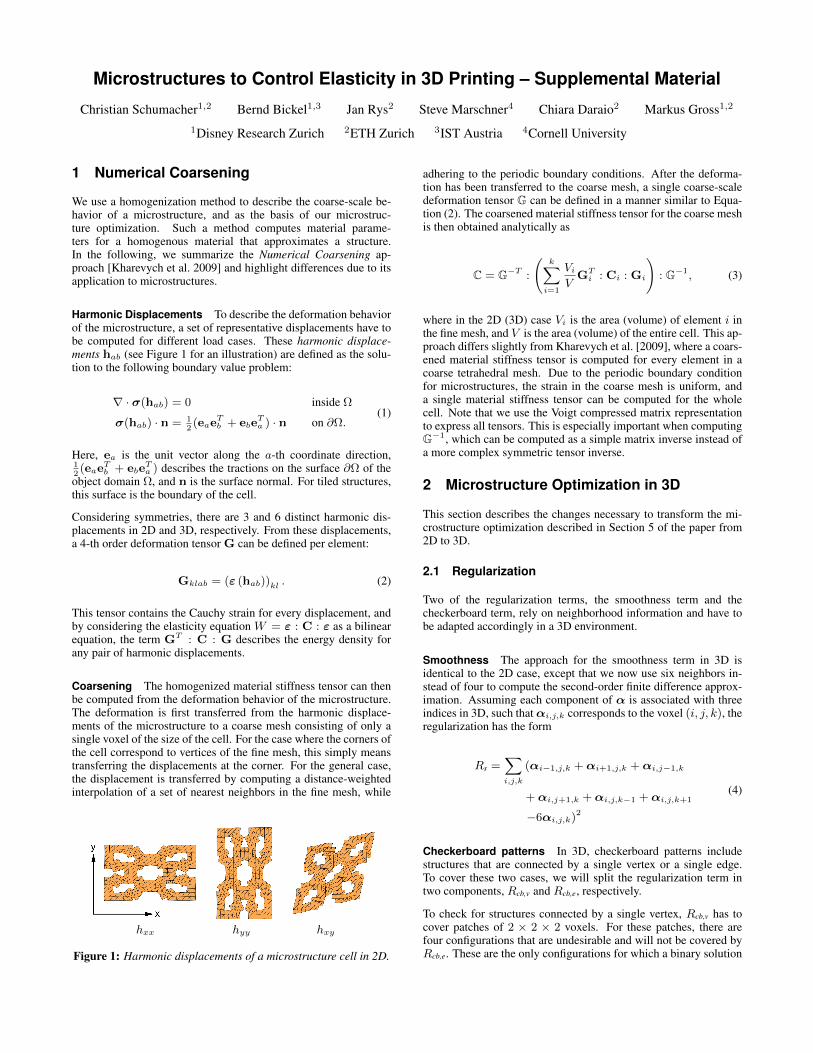
Coarsening The homogenized material stiffness tensor can thenbe computed from the deformation behavior of the microstructure.The deformation is first transferred from the harmonic displace-ments of the microstructure to a coarse mesh consisting of only asingle voxel of the size of the cell. For the case where the corners ofthe cell correspond to vertices of the fine mesh, this simply meanstransferring the displacements at the corner. For the general case,the displacement is transferred by computing a distance-weightedinterpolation of a set of nearest neighbors in the fine mesh, while

hxx hyy hxy

Figure 1: Harmonic displacements of a microstructure cell in 2D.

adhering to the periodic boundary conditions. After the deforma-tion has been transferred to the coarse mesh, a single coarse-scaledeformation tensor G can be defined in a manner similar to Equa-tion (2). The coarsened material stiffness tensor for the coarse meshis then obtained analytically as

C = G−T :

(k∑

i=1

Vi

VGT

i : Ci : Gi

): G−1, (3)

where in the 2D (3D) case Vi is the area (volume) of element i inthe fine mesh, and V is the area (volume) of the entire cell. This ap-proach differs slightly from Kharevych et al. [2009], where a coars-ened material stiffness tensor is computed for every element in acoarse tetrahedral mesh. Due to the periodic boundary conditionfor microstructures, the strain in the coarse mesh is uniform, anda single material stiffness tensor can be computed for the wholecell. Note that we use the Voigt compressed matrix representationto express all tensors. This is especially important when computingG−1, which can be computed as a simple matrix inverse instead ofa more complex symmetric tensor inverse.

2 Microstructure Optimization in 3D

This section describes the changes necessary to transform the mi-crostructure optimization described in Section 5 of the paper from2D to 3D.

2.1 Regularization

Two of the regularization terms, the smoothness term and thecheckerboard term, rely on neighborhood information and have tobe adapted accordingly in a 3D environment.

Smoothness The approach for the smoothness term in 3D isidentical to the 2D case, except that we now use six neighbors in-stead of four to compute the second-order finite difference approx-imation. Assuming each component of α is associated with threeindices in 3D, such thatαi,j,k corresponds to the voxel (i, j, k), theregularization has the form

Rs =∑i,j,k

(αi−1,j,k +αi+1,j,k +αi,j−1,k

+αi,j+1,k +αi,j,k−1 +αi,j,k+1

−6αi,j,k)2

(4)

Checkerboard patterns In 3D, checkerboard patterns includestructures that are connected by a single vertex or a single edge.To cover these two cases, we will split the regularization term intwo components, Rcb,v and Rcb,e, respectively.

To check for structures connected by a single vertex, Rcb,v has tocover patches of 2 × 2 × 2 voxels. For these patches, there arefour configurations that are undesirable and will not be covered byRcb,e. These are the only configurations for which a binary solution

should lead to a regularization value larger than 0. This conditioncan be formulated as

Rcb,e =∑i,j,k

(αi,j,k −αmin)(1−αi+1,j,k)

(1−αi,j+1,k)(1−αi,j,k+1)

(1−αi+1,j+1,k)(1−αi+1,j,k+1)

(1−αi,j+1,k+1)(αi+1,j+1,k+1 −αmin)

+(1−αi,j,k)(αi+1,j,k −αmin)

(1−αi,j+1,k)(1−αi,j,k+1)

(1−αi+1,j+1,k)(1−αi+1,j,k+1)

(αi,j+1,k+1 −αmin)(1−αi+1,j+1,k+1)

+(1−αi,j,k)(1−αi+1,j,k)

(αi,j+1,k −αmin)(1−αi,j,k+1)

(1−αi+1,j+1,k)(αi+1,j,k+1 −αmin)

(1−αi,j+1,k+1)(1−αi+1,j+1,k+1)

+(1−αi,j,k)(1−αi+1,j,k)

(1−αi,j+1,k)(αi,j,k+1 −αmin)

(αi+1,j+1,k −αmin)(1−αi+1,j,k+1)

(1−αi,j+1,k+1)(1−αi+1,j+1,k+1)

(5)

Structures that are connected by a single edge can be detected bylooking at patches of 2× 2× 1 voxels, similar to the regularizationin 2D. The only

Rcb,v =∑i,j,k

(1−αi,j,k)(αi+1,j,k −αmin)

(αi,j+1,k −αmin)(1−αi+1,j+1,k)

+(αi,j,k −αmin)(1−αi+1,j,k)

(1−αi,j+1,k)(αi+1,j+1,k −αmin)

+(1−αi,j,k)(αi+1,j,k −αmin)

(αi,j,k+1 −αmin)(1−αi+1,j,k+1)

+(αi,j,k −αmin)(1−αi+1,j,k)

(1−αi,j,k+1)(αi+1,j,k+1 −αmin)

+(1−αi,j,k)(αi,j+1,k −αmin)

(αi,j,k+1 −αmin)(1−αi,j+1,k+1)

+(αi,j,k −αmin)(1−αi,j+1,k)

(1−αi,j,k+1)(αi,j+1,k+1 −αmin)

(6)

3 Numerical Methods

The indirect relationship between the coarsened stiffness tensorC(h(α)) and the activationsα through the harmonic displacementsh(α) defined in Equation (1) has to be taken into account whencomputing the derivatives of the microstructure optimization prob-lem introduced in the paper. When the chain rule is applied to thisproblem, the Jacobian of the harmonic displacements with respectto the activations emerges. Since these quantities are effectivelylinked by the solution of an elasticity problem, given the boundarytractions defined in (1), we use the adjoint method to compute theJacobian. For this, we take the derivatives of both the minimization

condition∇xUel = 0 and the constraints c = 0 with respect to α:

∂2Uel

∂hab ∂α+

∂2Uel

∂hab2

dhab

dα= 0

∂c

∂hab

dhab

dα= 0.

(7)

Solving this system of equations for the desired Jacobian dhab/dαrequires only a single sparse matrix decomposition.

4 Compression Test Data

0 0.005 0.01 0.015 0.02 0.025 0.03−0.1

0

0.1

0.2

0.3

0.4

0.5

0.6

Engineering strain [−]

Str

ess [

MP

a]

base material

20.51x − 0.08

0 0.05 0.1 0.15−0.1

0

0.1

0.2

0.3

0.4

0.5

0.6

0.7

Engineering strain [−]

Str

ess [

MP

a]

structure A

4.41x − 0.03

0 0.01 0.02 0.03 0.04 0.05−0.01

0

0.01

0.02

0.03

0.04

0.05

0.06

Engineering strain [−]

Str

ess [

MP

a]

structure B

1.39x − 0.01

0 0.05 0.1 0.15−0.1

0

0.1

0.2

0.3

0.4

Engineering strain [−]

Str

ess [

MP

a]

structure C

2.51x − 0.02

Figure 2: The stress–strain measurements for the base materialand the three structures tested in the compression test. The tangentsof the linear part of the curve describes the Young’s modulus of thestructure.

Figure 2 shows the data from the compression tests of the base ma-terial and three synthesized structure. We determined the Young’smodulus of the structures by fitting a linear polynomial to the linearpart of the stress–strain curve.

References

KHAREVYCH, L., MULLEN, P., OWHADI, H., AND DESBRUN,M. 2009. Numerical coarsening of inhomogeneous elastic ma-terials. ACM Trans. Graph. (Proc. SIGGRAPH) 28, 51.