microswimmers near surfaces - springer · 2336 theeuropeanphysicaljournalspecialtopics fig. 3....

Eur. Phys. J. Special Topics 225, 2333–2352 (2016)© The Author(s) 2016DOI: 10.1140/epjst/e2016-60070-6

THE EUROPEANPHYSICAL JOURNALSPECIAL TOPICS

Regular Article

Microswimmers near surfaces

Jens Elgetia and Gerhard Gompperb

Theoretical Soft Matter and Biophysics,Institute of Complex Systems & Institute for Advanced Simulation,Forschungszentrum Julich, D-52425 Julich, Germany

Received 4 March 2016 / Received in final form 17 May 2016Published online 10 November 2016

Abstract. Both, in their natural environment and in a controlled exper-imental setup, microswimmers regularly interact with surfaces. Thesesurfaces provide a steric boundary, both for the swimming motion andthe hydrodynamic flow pattern. These effects typically imply a strongaccumulation of microswimmers near surfaces. While some generic fea-tures can be derived, details of the swimmer shape and propulsionmechanism matter, which give rise to a broad range of adhesion phe-nomena and have to be taken into account to predict the surface accu-mulation for a given swimmer. We show in this minireview how numer-ical simulations and analytic theory can be used to predict the accu-mulation statistics for different systems, with an emphasis on swimmershape, hydrodynamics interactions, and type of noisy dynamics.

1 Introduction

Lord Rothschild discovered already in 1963, more than 50 years ago, that live humansperm cells accumulate at surfaces, while dead cells do not [1]. Thus, classical at-tractive interactions, like electrostatic and van der Waals interactions, or interactionsmediated by receptor-ligand binding, are unlikely candidates for this surface accumu-lation. Since then, a similar behaviour has been observed for several other swimmingmicro-organisms, such as sperm of other species like bull [2] and sea-urchin, and bac-teria like E. coli [3,4]. Thus, surface accumulation seems to be a generic behaviourof microswimmers. This calls for a general physical description of this phenomenon[5]. Furthermore, although surface accumulation seems to be generic, it does not haveto be identical for all self-propelled particles. They could be closer to the surface orfurther away, and their retention time at the surface can be long or short.A detailed understanding of the surface accumulation of microswimmers is relevant

in a large number of current and future applications [5–8]. Biological micro-organismsfind many surfaces in their natural environments. For example, mammal sperm hasto move through the oviduct to reach the egg. Sperm of many fishes can enter theegg only at a particular spot, the micropyle, and thus has to locate it on the surface.Bacteria move along surfaces where they form colonies and biofilms [9]. Surfaces, in

a e-mail: [email protected] e-mail: [email protected]

http://www.epj.org/

http://dx.doi.org/10.1140/epjst/e2016-60070-6

2334 The European Physical Journal Special Topics

Fig. 1. Clover-leaf structures in microchannels can be employ to rectify microswimmermotion. Particles moving in the wrong direction follow the surface of the leaf at are therebyredirected by 180o. From Ref. [10]. (This figure is subject to copyright protection and is notcovered by a Creative Commons license.)

particular in microfluidic devices, can also be used to control and direct the motionof natural and artificial microswimmers [5]. For example, clover-shaped segments ina microchannel can work as a rectifier [10], see Fig. 1. Also, swimming along surfacesstrongly affects motion in curved microchannels [11], which can be used for particlesorting.How do microswimmers interact with surfaces? Several mechanisms are possible.

The first and probably most obvious way of a self-propelled particle to encountera surface is by self-propulsion. As an active particle moves through the embeddingmedium, or on a substrate, it will sooner or later approach a confining wall, andwill collide with it. Now, an active particle typically is subject to some noise, whichcan be either passive (thermal) or active. Therefore, it has some orientational persis-tence, i.e. it keeps pushing in the same direction for some time related to the inverserotational diffusion constant. During this time, the particle remains at the wall ormoves parallel to the wall, which implies an increased particle density near or at thewall. Thus, the competition of self-propulsion and orientational fluctuations inducesan effective wall adhesion. This behavior strongly depends on the particle shape andtype of orientational dynamics, as discussed in detail in Sect. 2. Here, highly ideal-ized model systems are considered, which are employed to elucidate general physicalprinciples of self-propulsion and shape. Self-propelled Brownian rods are discussed inSect. 2.1, active Brownian spheres in Sect. 2.2, active asymmetric Brownian dumb-bells in Sect. 2.3, and run-and-tumble particles in Sect. 2.4.It is worth mentioning that active Brownian particles have become a standard

model of self-propelled particles with noisy dynamics, in particular for studies ofmotility-induced phase separation and collective dynamics, see recent reviews [5,12],and minireview [13] by T. Speck in this issue.A second mechanisms is due to hydrodynamic interactions. As a microswimmer

usually swims in an aqueous environment, it sets the surrounding fluid into motion asit pushes itself forward. Since the fluid motion is affected by the presence of nearbyboundaries, the fluid mediates an interaction between microswimmers and walls. Theeffects of hydrodynamic interaction on the surface accumulation and swimming be-havior are described in Sect. 3. This interaction is rather simple in the far-field, whenthe distance of the microswimmer from the wall is much larger than the size of themicroswimmer itself, but becomes rather complex as the microswimmer comes closeto the surface, as discussed in Sect. 3.1. In particular, the behavior now depends onthe details of the swimming mechanism, such as the snake-like motion of sperm cells,or the corkscrew-like motion of bacteria flagella, as discussed in Sects 3.2 and 3.3,respectively.

Microswimmers – From Single Particle Motion to Collective Behaviour 2335

Fig. 2. (Left) Probability density P (z) as function of the distance z from the surface, forvarious propelling forces ft. The rod length is L � 10a (where a is the rod diameter), thewalls are located at z = 0 and z = 5L. A solid gray line shows the density profile of passiverods. (Right) Surface excess s as a function of scaled rod length L/a, for various propellingforces ft, as indicated. The (black) dashed-dotted line is the scaling result in the ballisticregime (see Eq. (4)), the (gray) dashed lines are scaling results in the diffusive regime forft = 0.5 and ft = 0.05. From Ref. [15]. (This figure is subject to copyright protection and isnot covered by a Creative Commons license.)

2 Active Brownian particles near surfaces: Self-Propulsion, noise,and shape matter

2.1 Self-propelled rods near surfaces

In order to elucidate the effect of shape on the wall adhesion of a self-propelled particledue to steric interactions, it is interesting to consider the behaviour of self-propelledBrownian rods near walls — in the absence of any hydrodynamic interactions, butwith Brownian noise (see also minireview [14] by F. Peruani in this issue). In thiscase, excluded-volume interactions favor parallel orientation along the wall, whilethe thermal noise leads to fluctuations of the rod orientation and thereby an effectiverepulsion from the wall. The competition of these two effects gives rise to an interestingadsorption behaviour [15,16].Very close to the wall, the rod has access to less orientational conformations.

This leads to an entropic repulsion from the wall for passive Brownian rods. Resultsof Brownian Dynamics simulations [15] are shown in Fig. 2. While passive rods aredepleted from the surface as expected, active rods show an increased probabilitydensity near the surface, which grows with increasing propelling force density ft, seeFig. 2(left). In addition to the propelling force, the behaviour of the rods stronglydepends on the rod length L. The surface excess — the integrated probability densityto find a rod near the surface compared to a uniform density distribution — is shownin Fig. 2(right). The results show that (i) propulsion always leads to an increases insurface excess, and (ii) depending on ft, the surface excess initially decreases withincreasing L, but than increases again to reach a plateau nearly independent of ftand L for large propelling forces and rod lengths [15]. In comparison with activeBrownian spheres (see Sect. 2.2 below), it is interesting to note that for rods, thesurface excess never reaches unity. Thus, the elongated shape leads to a reduction ofsurface accumulation due to rapid alignment with the surface upon collision.In order to understand the mechanism which is responsible for the effective surface

adhesion of self-propelled rods, and to predict their behaviour as a function of rodlength, propulsive force, and wall separation, the analogy of the trajectories of self-propelled rods with the conformations of semi-flexible polymers can be exploited [15].


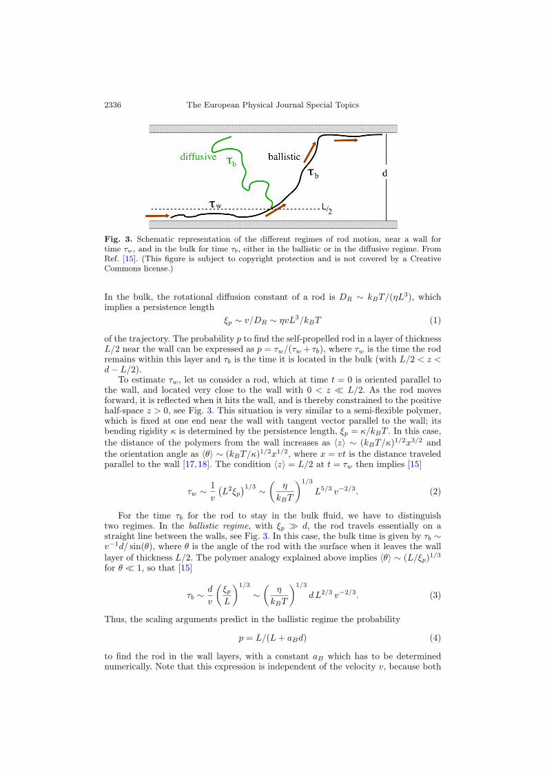
Fig. 3. Schematic representation of the different regimes of rod motion, near a wall fortime τw, and in the bulk for time τb, either in the ballistic or in the diffusive regime. FromRef. [15]. (This figure is subject to copyright protection and is not covered by a CreativeCommons license.)

In the bulk, the rotational diffusion constant of a rod is DR ∼ kBT/(ηL3), whichimplies a persistence length

ξp ∼ v/DR ∼ ηvL3/kBT (1)

of the trajectory. The probability p to find the self-propelled rod in a layer of thicknessL/2 near the wall can be expressed as p = τw/(τw + τb), where τw is the time the rodremains within this layer and τb is the time it is located in the bulk (with L/2 < z <d− L/2).To estimate τw, let us consider a rod, which at time t = 0 is oriented parallel to

the wall, and located very close to the wall with 0 < z � L/2. As the rod movesforward, it is reflected when it hits the wall, and is thereby constrained to the positivehalf-space z > 0, see Fig. 3. This situation is very similar to a semi-flexible polymer,which is fixed at one end near the wall with tangent vector parallel to the wall; itsbending rigidity κ is determined by the persistence length, ξp = κ/kBT . In this case,

the distance of the polymers from the wall increases as 〈z〉 ∼ (kBT/κ)1/2x3/2 andthe orientation angle as 〈θ〉 ∼ (kBT/κ)1/2x1/2, where x = vt is the distance traveledparallel to the wall [17,18]. The condition 〈z〉 = L/2 at t = τw then implies [15]

τw ∼ 1v

(L2ξp

)1/3 ∼(η

kBT

)1/3L5/3 v−2/3. (2)

For the time τb for the rod to stay in the bulk fluid, we have to distinguishtwo regimes. In the ballistic regime, with ξp � d, the rod travels essentially on astraight line between the walls, see Fig. 3. In this case, the bulk time is given by τb ∼v−1d/ sin(θ), where θ is the angle of the rod with the surface when it leaves the walllayer of thickness L/2. The polymer analogy explained above implies 〈θ〉 ∼ (L/ξp)1/3for θ � 1, so that [15]

τb ∼ dv

(ξp

L

)1/3∼(η

kBT

)1/3dL2/3 v−2/3. (3)

Thus, the scaling arguments predict in the ballistic regime the probability

p = L/(L+ aBd) (4)

to find the rod in the wall layers, with a constant aB which has to be determinednumerically. Note that this expression is independent of the velocity v, because both


Fig. 4. Schematic of active Brownian spheres moving near a surface. From Ref. [20]. (Thisfigure is subject to copyright protection and is not covered by a Creative Commons license.)

time scales τw and τb depend on v in the same way. Thus, scaling theory explains thesaturation of the excess surface density with increasing propelling force, as shown inFig. 2(right).For a system of many self-propelled Brownian rods between two walls in two

dimensions, the rods moving along the walls in opposite directions block each otherand lead to the formation of “hedgehog-like” clusters [19].

2.2 Active Brownian spheres in confinement

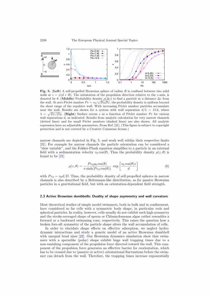
We have seen in the previous section that the alignment of rods with the surfaceplays an important role in their behaviour near surfaces. What happens if no suchalignment mechanism is present? This question can be addressed by studying self-propelled Brownian spheres, where the sphere orientation is completely independentof their spatial position, while the propulsion still drives the particles toward thewalls, as shown schematically in Fig. 4.Results of Brownian Dynamics simulations of active Brownian spheres in confine-

ment between two hard walls are presented in Fig. 5. where the surface excess s isshown as a function of the Peclet number Pe = v0/

√DRDT for different channel

widths. These results demonstrate that the (normalized) probability density ρ(Δz)to find a particle at a distance Δz from the wall is strongly peaked close to the wallfor Pe � 5. Note that s is a monotonically increasing function of Pe, and approachesunity for large Pe (complete adhesion).The decoupling of the rotational degrees of freedom from translational motion

allows for an analytic treatment via the Fokker-Planck equation [21]

∂tρ(z, θ, t) = DR1

sin(θ)∂θ [sin(θ)∂θρ(z, θ, t)]− v0 cos(θ)∂zρ(z, θ, t) +DT∂2zρ(z, θ, t),

(5)where the angle θ = 0 corresponds to particles oriented in the positive z-direction.This equation already demonstrates the main origin of surface accumulation. Therotational diffusion is independent of the spatial position, but particles are drivento one of the chamber walls depending on their orientation. Thus particles orientedtoward the top, accumulate at the top wall, those pointing down, accumulate at thebottom wall. Less particles remain in the center. Solutions for small Peclet number and


0

0.2

0.4

0.6

0.8

1

1.2

0 0.5 1 1.5

ρ

Δz/λ

Pe=0.00Pe=1.46Pe=7.30Pe=14.6

R0

z

−d

+dR

R

θ

0

0.2

0.4

0.6

0.8

1

0.1 1 10 100 1000

s

Pe

d=0.45λd=2.23λd=15.6λ

Fig. 5. (Left) A self-propelled Brownian sphere of radius R is confined between two solidwalls at z = ±(d + R). The orientation of the propulsion direction relative to the z-axis, isdenoted by θ. (Middle) Probability density ρ(Δz) to find a particle at a distance Δz fromthe wall. At zero Peclet number Pe = v0/

√DRDT , the probability density is uniform beyond

the short range of the repulsive wall. With increasing Peclet number particles accumulatenear the wall. Results are shown for a system with wall separation d/λ = 15.6, where

λ =√DT /DR. (Right) Surface excess s as a function of Peclet number Pe for various

wall separations d, as indicated. Results from analytic calculation for very narrow channels(dotted lines) and for small Peclet numbers (dashed lines) are also shown. All analyticexpression have no adjustable parameters. From Ref. [21]. (This figure is subject to copyrightprotection and is not covered by a Creative Commons license.)

narrow channels are depicted in Fig. 5, and work well within their respective limits[21]. For example for narrow channels the particle orientation can be considered a“slow variable”, and the Fokker-Plank equation simplifies to a particle in an externalfield with a sedimentation velocity v0 cos(θ). Thus the probability density ρ(z, θ) isfound to be [21]

ρ(z, θ) =Pedρ0 cos(θ)

π sinh(Ped cos(θ))exp

[v0 cos(θ)z

d

](6)

with Ped = v0d/D. Thus, the probability density of self-propelled spheres in narrowchannels is also described by a Boltzmann-like distribution, as for passive Brownianparticles in a gravitational field, but with an orientation-dependent field strength.

2.3 Active Brownian dumbbells: Duality of shape asymmetry and wall curvature

Most theoretical studies of simple model swimmers, both in bulk and in confinement,have considered so far cells with a symmetric body shape, in particular rods andspherical particles. In reality, however, cells usually do not exhibit such high symmetryand the stroke-averaged shape of sperm or Chlamydomonas algae rather resembles aforward or a backward swimming cone, respectively. This raises the question how abroken fore-aft symmetry of the particle shape alters the wall accumulation of cells.In order to elucidate shape effects on effective adsorption, we neglect hydro-

dynamic interactions and study a generic model of an active Brownian dumbbellwith unequal bead sizes [22]. Our Brownian dynamics simulation show that swim-mers with a spermlike (polar) shape exhibit huge wall trapping times due to anon-vanishing component of the propulsion force directed toward the wall. This com-ponent of the propulsion force generates an effective barrier for reorientation, whichhas to be crossed due to (passive or active) orientational fluctuations before the swim-mer can detach from the wall. Therefore, the trapping times increase exponentially


R → ∞ R → ∞

θ0

θ0

R(a)

(b)

Fig. 6. (a) An apolar swimmer confined within a spherical cavity of radius R is equivalent toa polar swimmer close to a flat wall – provided the angle θ0 � −l/2R between the propulsionforce of the apolar swimmer and the tangent plane of the cavity at the front bead, equalsthe asymmetry (opening angle) θ0 � (a1 − a2)/l of the polar particle, where a1 and a2 arethe radii of the rear and front bead of the dumbbell, respectively, and l is the bond length.(b) A polar particle near a convex boundary behaves like an apolar swimmer close to a flatwall if (a1 − a2)/l � −l/2R. From Ref. [22]. (This figure is subject to copyright protectionand is not covered by a Creative Commons license.)

with the shape asymmetry (opening angle) θ0 and the propulsion strength (free-swimming velocity) V and could, for realistic parameters of θ0 and V , exceed trappingtimes due to near-field hydrodynamic forces [15,23,24]. In contrast, microswimmerswith Chlamydomonas-like (antipolar) shape behave similarly to symmetric rod-likeparticles.Both in a natural environment and in microfluidic devices, microswimmers usually

do not swim in straight, but rather in curved or branching microchannels. Therefore,the influence of surface curvature on accumulation of microswimmers is of great in-terest [25]. Based on the analysis of an asymmetric particle near a flat boundary,we can predict a direct duality relation between the effect of shape asymmetry andsurface curvature on accumulation, as illustrated in Fig. 6. For example, a polar mi-croswimmer close to a flat wall behaves similarly to an apolar particle near a concavesurface (e.g., a cavity), see Fig. 6(a). In both cases, the velocity vector in the stableconformation forms an angle with the tangent plane to the wall at the front bead,so that the microswimmer points toward the wall and thus should have very longretention times [22]. Second, the force of a polar microswimmer towards the wall canbe partially or fully compensated by a convex wall, i.e., for a microswimmer movingat the outer surface of a sphere of radius R, see Fig. 6(b). For full compensation,the same accumulation behaviour is predicted as for an apolar particle at a planarwall. Note that, in contrast, an apolar microswimmer would strongly scatter at a con-vex wall. Thus, shape polarity provides the possibility for microswimmers to movealong curved surfaces. This is of high relevance for the design of microswimmers withcontrolled wall-adhesion properties.

2.4 Run-and-tumble particles in confinement

The simplification from a swimmer in confinement to a self propelled rod or sphere,can be taken even another step further. The run-and-tumble dynamics famous fromE. coli chemotaxis [27] is in its idealized form of a random walker with finite steplength well suited for mathematical treatment.


0.3

0.4

0.5

0.6

0 0.2 0.4 0.6 0.8 1

ρ

z/d

3-D L=2d 2-D L=d/22-D L=d 2-D L=2d

z

z*

Θvτr =L

−d

0

+d

Fig. 7. (left) Schematic of run-and-tumble dynamics. A “run” of the particle with a velocityv for a time τr is followed by a tumbling event, resulting in a new orientation θ. The particleis confined between two parallel walls at z = ±d. z∗ denotes the distance from the walls.(right) Particle density distribution ρ(z) for various run lengths L. The solid line is theexact analytic solution for the particle density in three dimensions for run lengths largerthan the channel width 2d. From Ref. [26]. (This figure is subject to copyright protectionand is not covered by a Creative Commons license.)

During chemotaxis, E. coli swim in relative straight “runs” followed by “tumblingevents” in which the bacterium reorients. The idealized version (see Fig. 7) we willstudy here, is similar to a random walk or Levy flight. During the instantaneoustumbling event, the swimmer chooses a direction completely at random. The followingstraight run lasts either for a fixed time τ , or is chosen from an exponential distributionwith mean τ .In the bulk, far from surfaces, it has been shown that run-and-tumble dynamics

and active Brownian motion are equivalent [28–30]. Even in slowly varying externalpotential U(z), this equivalence holds. For example, the density distribution is foundto be [28]

ρ(z) ∼ exp[−βU(z)], with β = μαv20=μ

D, (7)

where α is the tumbling rate, μ the particle mobility (the inverse friction coefficient),and D = v20/(αd) the diffusivity (for spatial dimensionality d). This is exactly thesame functional form of the Boltzmann distribution in thermal equilibrium, but nowwith an effective temperature kBTeff = 1/β. This effective temperature is typicallymuch larger than the thermodynamic temperature for self-propelled particles. How-ever, this equivalence breaks down in the vicinity of walls and surfaces [26].For the study of run-and-tumble motion near walls and in confinement [26], we

do not study the particle density, but the density of tumbling events Φ. As tumblingevents have no orientation, the tumbling density only depends on the distance to thesurface z. We arrive thus at an one-dimensional problem. The particle orientationis effectively integrated out. The actual particle density can be obtained from thetumbling density by a convolution integral. Alternatively, it is also possible to workdirectly with the combined particle-orientation density [31]. While a bit more involved,it offers direct access to the mean particle orientation.The Fokker-Planck equation for the tumbling density can be obtained from simple

considerations. A particle tumbling at a distance to the surface z will choose a randomorientation and run straight for a distance L = v0τ . This results in a new position a−Δz an the process starts anew. If we call the probability of a certain z−displacement(or transfer function) p(Δz), the tumbling event density evolves as [26]

φ(z, t+ τr) =

∫ +d

−dφ(z′, t)p(z − z′)dz′. (8)


This however does not include the solid boundaries yet. In these dynamics however,this is rather simple. Particles just can not penetrate the wall, that is to say, if theyhit the wall they remain there. This results in a delta peak of the tumbling densityat the wall,

φ(±d, t) = 0.5φs(t)δ(z ± d) (9)

0.5φs(t+ τr) =

∫ d

−dφ(z′, t)P (−z′ − d)dz′ (10)

where φs is the probability to find a tumbling event at the wall, and P is the cumu-lative distribution function of p, i.e. P (z) =

∫ z−∞ p(z

′)dz′.Already from this simple intermediate result, we see that run-and-tumble particles

will accumulate at the wall. In a rather thin channel it is quite simple: A particletumbles at the wall. Half the time it just remains at the wall, in the rest of the cases,there is a high chance, that the run carries the particle straight over to the other wall.Thus most of the tumbling events happen at the wall.To calculate this in more detail, one has to obtain the transfer function. The trans-

fer function is the number of microstates (possible orientations), which are compatiblewith a certain displacement Δz perpendicular to the wall. The number of microstatesis proportional to the fraction of the surface area of the sphere of motion vectors,which generates a vertical displacement Δz. For example, in the case of constant runlength L in three dimensions, the transfer function is thus determined by [26]

p(z)dz =1

4πL2

∫ 2π

0

dϕ

∫ arccos(z)

arccos(z+dz)

dθ L sin(θ)

= − 12Lcos(θ)|arccos(z)arccos(z+dz)

=1

2Ldz

for |z| < L. Thus, the transition probability for vertical displacements is uniform inthree dimensions. In two dimensions, an equivalent derivation shows that the transferfunction diverges instead at ±L

p(2,c)(z) =1

πL√1− (z/L)2Θ(L− z)Θ(L+ z). (11)

The discontinuity at Δz = ±L leads to peaks and interference patterns in the tum-bling density (see Fig. 8). The simplicity of the 3D transfer function allows for ananalytic solution for narrow channels with 2d < L,

φ(3,c)(z) =1

2L+1− d/L2

[δ(z − d) + δ(z + d)] (12)

The solution for two dimensions or larger channel widths can only be obtained withcertain simplifications. See Ref. [26] for more details.In the case of more general run length distributions, one simply uses the condi-

tional probability to obtain the transfer function:

p(n,len)(z) =

∫ ∞

z

P(n,c)(z|L′)plen(L′)dL′ (13)


0

0.2

0.4

0.6

0.001 0.01 0.1 1 10 100

φ s d

/L

d/L

2D

α/2

α/2

exponentialconstant

0.7

0.8

0.9

1

0.01 0.1 1

φ s

0

0.2

0.4

0.6

0.001 0.01 0.1 1 10 100

φ s d

/L

d/L

3D

α/2

α/2

exponentialconstant

0.7

0.8

0.9

1

0.01 0.1

φ s

-1 -0.5 0 0.5 1z/d

0

1

2

L/d

0.4

0.6

0.8

1

1.2

1.4

0.6

0.8

1

1.2

1.4

0 0.5 1 1.5 2 2.5

φ/φ b

z*/L

2D

Exponential

Constant

d/L=2.5d/L=5

d/L=10d/L=2.5

d/L=5d/L=10

0.6

0.8

1

1.2

1.4

0 0.5 1 1.5 2 2.5

φ/φ b

z*/L

3D

Exponential

Constant

d/L=2.5d/L=5

d/L=10d/L=2.5

d/L=5d/L=10

-1 -0.5 0 0.5 1z/d

0

1

2

L/d

0.4

0.6

0.8

1

1.2

1.4

Fig. 8. Tumbling density profiles φ(z) for (top) two and (bottom) three dimensions. (left)Scaled surface density φsd/L as a function of the ratio d/L of channel width and run length.Solid lines are analytical approximations for narrow channels (see text), dashed lines are fitsto a large-channel approximation. Note that for d� L, (φsd/L) approaches α/2. (center)Scaled tumbling density φ(z∗)/φb as a function of the scaled distance z∗/L = (z+d)/L fromthe wall. Dashed lines show the approximation φ1(z

∗), which is obtained from a first-orderiteration of Eq. (8) (see text). (right) Density of tumbling events φ(z/L) inside the channelfor various (constant) run lengths. For 2d ≥ L, the presence of the two walls induces strongdensity modulations. From Ref. [26]. (This figure is subject to copyright protection and isnot covered by a Creative Commons license.)

with the run-length distribution plen(L′) For exponential run-length distributions, the

broadness of the run length distribution destroys the peaks and valleys away fromthe wall, and only an increased density at the wall is left (see Fig. 8).These calculations are, however, only valid for an idealized run-and-tumble dy-

namics. For the description of the behaviour of real bacteria, a certain persistence inthe tumbling events [32] and the influence of walls on tumbling frequency [33] probablyhas to be taken into account, and may significantly affect the results. Thus, it remainschallenging to understand and predict the dynamics of real E. coli in confinement.

3 Hydrodynamic interactions of microswimmers with surfaces

3.1 Microswimmer hydrodynamics

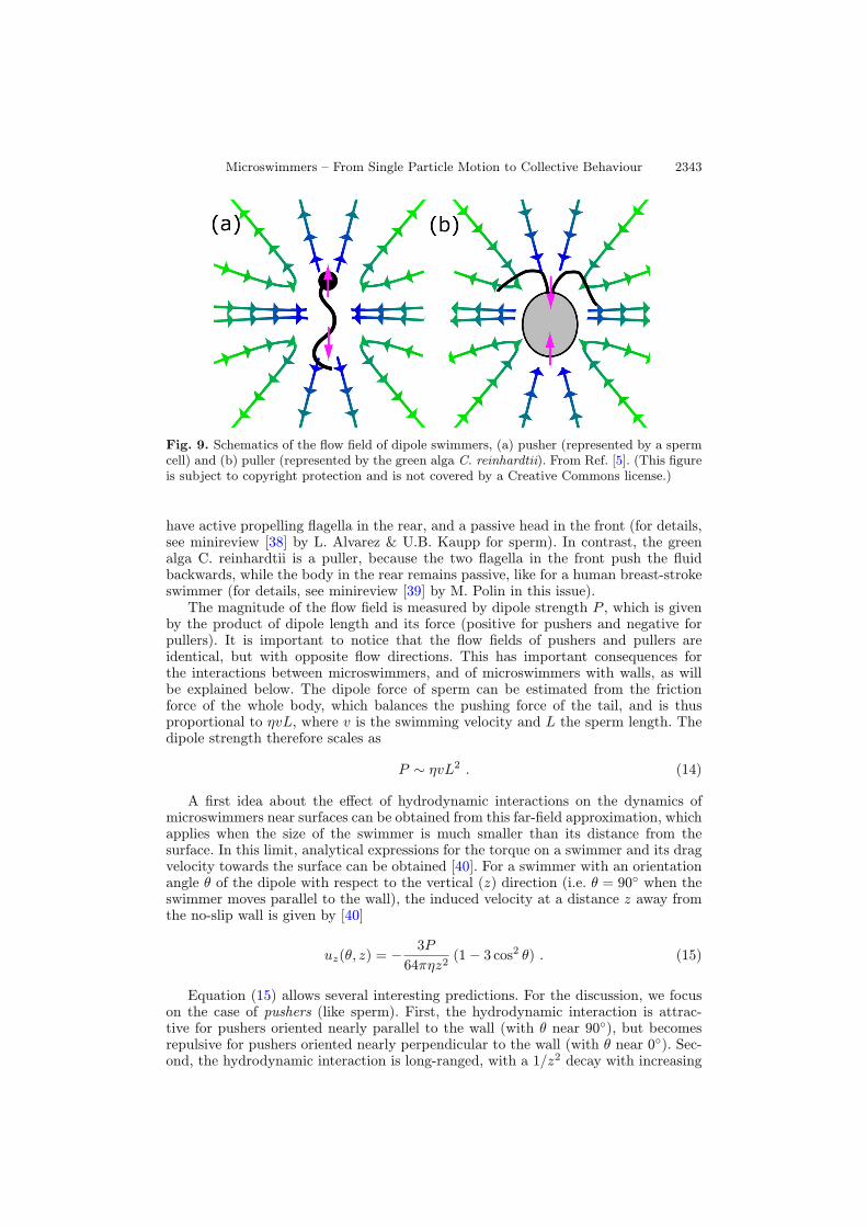
Most microswimmers move autonomously, with no external force applied, and hencethe total interaction force of the swimmer on the fluid, and vice versa, vanishes.In the simplest case, which actually applies to many microswimmers like bacteria,spermatozoa, or algae, the far-field hydrodynamics (at distances from the swimmermuch larger than its size) can be well described by a force dipole [34,35]. For a detaileddescription and discussion of the dipole flow field see minireview [36] by R.G. Winklerin this issue. This approximation has been confirmed experimentally for E. coli [37].Two classes of such dipole swimmers can be distinguished, as shown schematically inFig. 9. If the swimmer has its motor in the back, and the passive body drags alongthe surrounding fluid in front, the characteristic flow field of a “pusher” emerges, seeFig. 9(a). Similarly, if the swimmer has its motor in the front, and the passive bodydrags along the surrounding fluid behind, the characteristic flow field of a “puller”develops, see Fig. 9(b). Thus, sperm, E. coli and salmonella are pushers, because they


Fig. 9. Schematics of the flow field of dipole swimmers, (a) pusher (represented by a spermcell) and (b) puller (represented by the green alga C. reinhardtii). From Ref. [5]. (This figureis subject to copyright protection and is not covered by a Creative Commons license.)

have active propelling flagella in the rear, and a passive head in the front (for details,see minireview [38] by L. Alvarez & U.B. Kaupp for sperm). In contrast, the greenalga C. reinhardtii is a puller, because the two flagella in the front push the fluidbackwards, while the body in the rear remains passive, like for a human breast-strokeswimmer (for details, see minireview [39] by M. Polin in this issue).The magnitude of the flow field is measured by dipole strength P , which is given

by the product of dipole length and its force (positive for pushers and negative forpullers). It is important to notice that the flow fields of pushers and pullers areidentical, but with opposite flow directions. This has important consequences forthe interactions between microswimmers, and of microswimmers with walls, as willbe explained below. The dipole force of sperm can be estimated from the frictionforce of the whole body, which balances the pushing force of the tail, and is thusproportional to ηvL, where v is the swimming velocity and L the sperm length. Thedipole strength therefore scales as

P ∼ ηvL2 . (14)

A first idea about the effect of hydrodynamic interactions on the dynamics ofmicroswimmers near surfaces can be obtained from this far-field approximation, whichapplies when the size of the swimmer is much smaller than its distance from thesurface. In this limit, analytical expressions for the torque on a swimmer and its dragvelocity towards the surface can be obtained [40]. For a swimmer with an orientationangle θ of the dipole with respect to the vertical (z) direction (i.e. θ = 90◦ when theswimmer moves parallel to the wall), the induced velocity at a distance z away fromthe no-slip wall is given by [40]

uz(θ, z) = − 3P

64πηz2(1− 3 cos2 θ) . (15)

Equation (15) allows several interesting predictions. For the discussion, we focuson the case of pushers (like sperm). First, the hydrodynamic interaction is attrac-tive for pushers oriented nearly parallel to the wall (with θ near 90◦), but becomesrepulsive for pushers oriented nearly perpendicular to the wall (with θ near 0◦). Sec-ond, the hydrodynamic interaction is long-ranged, with a 1/z2 decay with increasing


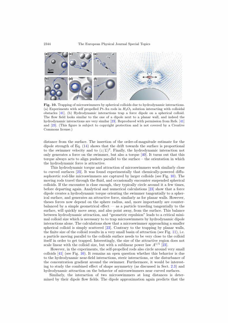
Fig. 10. Trapping of microswimmers by spherical colloids due to hydrodynamic interactions.(a) Experiments with self propelled Pt-Au rods in H2O2 solution interacting with colloidalobstacles [41]. (b) Hydrodynamic interactions trap a force dipole on a spherical colloid.The flow field looks similar to the one of a dipole next to a planar wall, and indeed thehydrodynamic interactions are very similar [23]. Reproduced with permission from Refs. [41]and [23]. (This figure is subject to copyright protection and is not covered by a CreativeCommons license.)

distance from the surface. The insertion of the order-of-magnitude estimate for thedipole strength of Eq. (14) shows that the drift towards the surface is proportionalto the swimmer velocity and to (z/L)2. Finally, the hydrodynamic interaction notonly generates a force on the swimmer, but also a torque [40]. It turns out that thistorque always acts to align pushers parallel to the surface – the orientation in whichthe hydrodynamic force is attractive.This hydrodynamic torque and attraction of microswimmers work similarly close

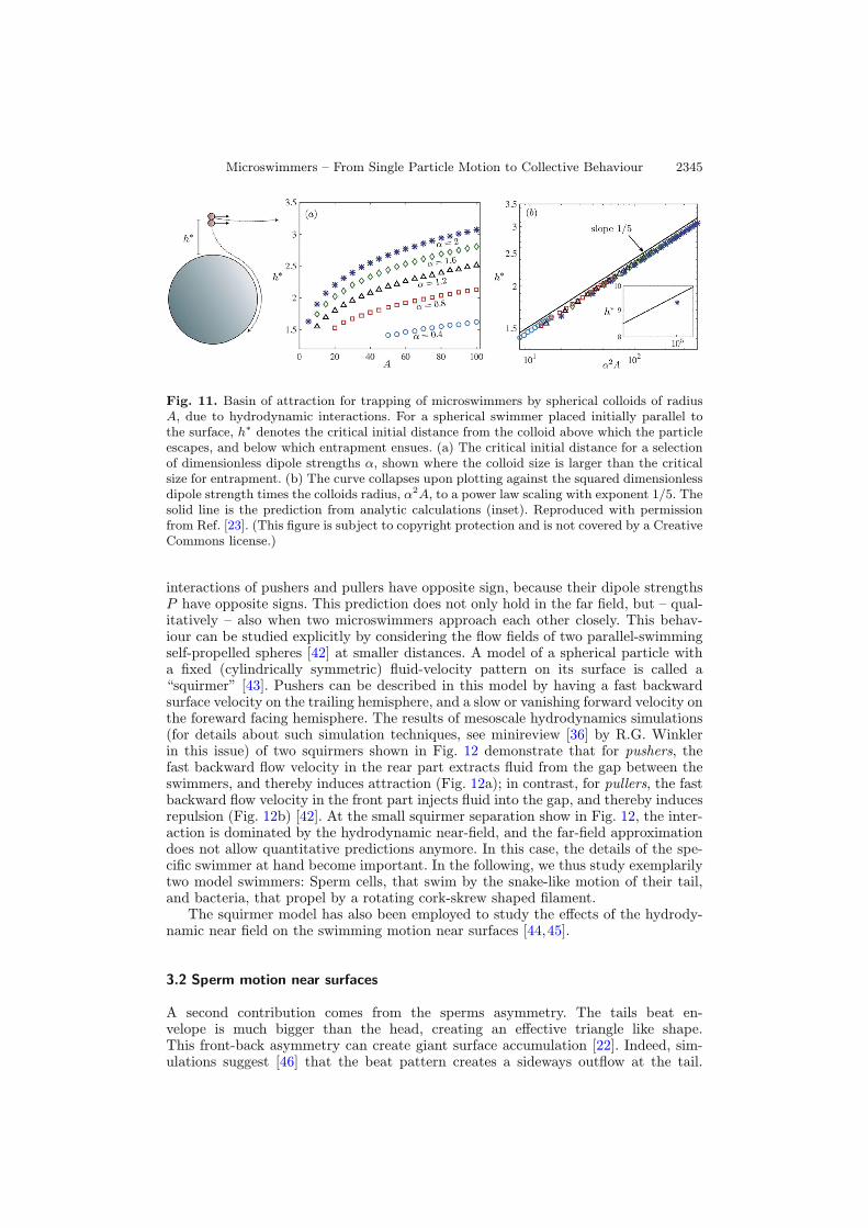
to curved surfaces [23]. It was found experimentally that chemically-powered diffu-sophoretic rod-like microswimmers are captured by larger colloids (see Fig. 10). Themoving rods travel through the fluid, and occasionally encounter suspended sphericalcolloids. If the encounter is close enough, they typically circle around it a few times,before departing again. Analytical and numerical calculations [23] show that a forcedipole creates a hydrodynamic torque orienting the swimmer tangentially to a spher-ical surface, and generates an attractive force, similarly as for planar walls. However,theses forces now depend on the sphere radius, and, more importantly are counter-balanced by a simple geometrical effect — as a particle traveling tangentially to thesurface, will quickly move away, and also point away, from the surface. This balancebetween hydrodynamic attraction, and “geometric repulsion” leads to a critical mini-mal colloid size which is necessary to to trap microswimmers by hydrodynamic dipoleinteractions alone. The calculations show that a microswimmer approaching a smallerspherical colloid is simply scattered [23]. Contrary to the trapping by planar walls,the finite size of the colloid results in a very small basin of attraction (see Fig. 11), i.e.a particle moving parallel to the colloids surface needs to be very close to the colloiditself in order to get trapped. Interestingly, the size of the attractive region does notscale linear with the colloid size, but with a sublinear power law A1/5 [23].However, in the experiments, the self-propelled rods also circle around very small

colloids [41] (see Fig. 10). It remains an open question whether this behavior is dueto the hydrodynamic near-field interactions, steric interactions, or the disturbance ofthe concentration gradient around the swimmer. Furthermore, it would be interest-ing to study the combined effect of shape asymmetry (as discussed in Sect. 2.3) andhydrodynamic attraction on the behavior of microswimmers near curved surfaces.Similarly, the interaction of two microswimmers at long distances is deter-

mined by their dipole flow fields. The dipole approximation again predicts that the


Fig. 11. Basin of attraction for trapping of microswimmers by spherical colloids of radiusA, due to hydrodynamic interactions. For a spherical swimmer placed initially parallel tothe surface, h∗ denotes the critical initial distance from the colloid above which the particleescapes, and below which entrapment ensues. (a) The critical initial distance for a selectionof dimensionless dipole strengths α, shown where the colloid size is larger than the criticalsize for entrapment. (b) The curve collapses upon plotting against the squared dimensionlessdipole strength times the colloids radius, α2A, to a power law scaling with exponent 1/5. Thesolid line is the prediction from analytic calculations (inset). Reproduced with permissionfrom Ref. [23]. (This figure is subject to copyright protection and is not covered by a CreativeCommons license.)

interactions of pushers and pullers have opposite sign, because their dipole strengthsP have opposite signs. This prediction does not only hold in the far field, but – qual-itatively – also when two microswimmers approach each other closely. This behav-iour can be studied explicitly by considering the flow fields of two parallel-swimmingself-propelled spheres [42] at smaller distances. A model of a spherical particle witha fixed (cylindrically symmetric) fluid-velocity pattern on its surface is called a“squirmer” [43]. Pushers can be described in this model by having a fast backwardsurface velocity on the trailing hemisphere, and a slow or vanishing forward velocity onthe foreward facing hemisphere. The results of mesoscale hydrodynamics simulations(for details about such simulation techniques, see minireview [36] by R.G. Winklerin this issue) of two squirmers shown in Fig. 12 demonstrate that for pushers, thefast backward flow velocity in the rear part extracts fluid from the gap between theswimmers, and thereby induces attraction (Fig. 12a); in contrast, for pullers, the fastbackward flow velocity in the front part injects fluid into the gap, and thereby inducesrepulsion (Fig. 12b) [42]. At the small squirmer separation show in Fig. 12, the inter-action is dominated by the hydrodynamic near-field, and the far-field approximationdoes not allow quantitative predictions anymore. In this case, the details of the spe-cific swimmer at hand become important. In the following, we thus study exemplarilytwo model swimmers: Sperm cells, that swim by the snake-like motion of their tail,and bacteria, that propel by a rotating cork-skrew shaped filament.The squirmer model has also been employed to study the effects of the hydrody-

namic near field on the swimming motion near surfaces [44,45].

3.2 Sperm motion near surfaces

A second contribution comes from the sperms asymmetry. The tails beat en-velope is much bigger than the head, creating an effective triangle like shape.This front-back asymmetry can create giant surface accumulation [22]. Indeed, sim-ulations suggest [46] that the beat pattern creates a sideways outflow at the tail.


Fig. 12. Velocity fields for a pair of squirmers with fixed distance and fixed parallel ori-entation, for (left) pusher and (right) puller, with Peclet number Pe = 1155. Swimmersmove to the right. Streamlines serve as a guide to the eye. Only a fraction of the simulationbox is shown. (Due to the finite resolution of the measured velocity field, some streamlines(unphysically) end on the squirmers’ surfaces.) From Ref. [42]. (This figure is subject tocopyright protection and is not covered by a Creative Commons license.)

This creates a repulsion of the tail, resulting in a torque, leading to the sperm cellpointing towards the wall. It was later confirmed experimentally that indeed spermseem to be swimming at the wall, with a small but finite angle pointing against thesurface [11].Thus the adhesion of sperm cells to surfaces is a combination of several different

contributions, and it is hard to identify which is the dominant one. Furthermore,sperm do not swim in straight lines, but typically on preferably right handed circles(see Fig. 14). Simulations show that a asymmetry in the head can be sufficient to ex-plain not only circular motion, but also the preferred handedness. One can speculatethat sperm use this kind of asymmetry to navigate towards the egg in drifting circles[47] or helices [48].Generic models can help to understand how different effects contribute to the

swimmer-surface interaction. However, each microswimmer has its own combinationof contributions, and often additional non universal effects matter. Sperm cells forexample swim very close to nearby walls. Indeed the distance to the wall is muchsmaller than the sperms length, rendering the multipole expansion invalid. Neverthe-less Sperm-cell-like beating close to a wall creates a flow field, very similar to that ofa pusher (see Fig. 13).The circular motion of sperm near surfaces also gives rise to an interesting collec-

tive behaviour at higher densities – where sperm form quite regular arrays of vorticesin which several sperm swim together in tight circles [49,50] – and in shear flow –where sperm align against the flow direction and can swim upstream with a fixeddeviation angle (rheotaxis) [51–53]. A discussion of more generic aspects of circleswimmers is given in the minireview [54] by H. Lowen in this issue; an overview ofthe behaviour of microswimmers in external (flow) fields is provided in the minireview[55] by H. Stark.


Fig. 13. Averaged flow field in the vicinity of a sperm cell adhering to a wall. (a) Planeperpendicular to the wall, and (b) plane parallel to the wall, with both planes containing theaverage sperm shape. A snapshot of a sperm is superimposed. The flow field generated bythe beating tail is directed away from the sperm along their swimming direction and towardsthe sperm along its side. From Ref. [46]. (This figure is subject to copyright protection andis not covered by a Creative Commons license.)

Fig. 14. (a) Sketch of forces responsible for the adhesion of sperm at a surface. Top: Withouthydrodynamic interactions, the beating-plane of adhering sperm is oriented perpendicular tothe surface. Bottom: With hydrodynamic interactions, the beating-plane is oriented parallelto the surface. (b) Sperm (model with curved and elastically deformable midpiece) with large

preferred curvature (c(m)0 Lm = 1) at a surface. The head touches the wall and blocks further

rotation. The beating plane is approximately perpendicular to the surface. From Ref. [46].(This figure is subject to copyright protection and is not covered by a Creative Commonslicense.)

3.3 Bacterial motion close to homogeneous and striped surfaces

Most bacteria exploit helical filaments for propulsion, driven by rotary motors locatedin their cell membrane. Prominent examples of peritrichous bacteria, which possessnumerous flagella, are Escherichia coli, Salmonella typhimurium, Rhizobium lupini,


(b)(a)

Fig. 15. (a) Flow and pressure fields, which develop for a rotating body near a planar orcurved wall. From Ref. [62]. (b) Definition of the Navier slip length b for simple shear flownear a solid wall. (This figure is subject to copyright protection and is not covered by aCreative Commons license.)

or Proteus mirabilis to name just a few. In a bulk fluid, the bacteria move in a straightmanner (run), with all flagella forming a bundle, interrupted by abrupt changes ofthe swimming direction (tumble) induced by disintegration of the bundle [27], asmentioned above. The presence of a surface drastically alters the swimming behaviour.For instance, the non-tumbling mutant of E. coli swims in a clockwise (CW) circulartrajectory close to a solid boundary [4,56] and a counterclockwise (CCW) trajectoryclose to a liquid-air interface [56–58]. Hence, bacteria are able to “sense” the propertiesof a nearby surface, an aspect of great importance for surface selection and attachmentin the early stages of biofilm formation or infection [4,59,60]. Also, a theoreticalunderstanding of hydrodynamic interactions between swimming bacteria and surfacesnot only sheds light on selective surface attachment, but opens an avenue for thedesign of microfluidic devices to control and guide bacterial motion [3] for separation,trapping, stirring, etc. [61].The swimming behaviour of bacteria near surfaces is governed by hydrodynamic

forces [5,34] and, hence, the CW and CCW circular trajectories of E. coli have to beexplained in terms of hydrodynamic interactions. The basic physical mechanism is asfollows. The rotary motors generate rotations of the flagellar bundle and of the cellbody in opposite directions, such that the whole swimmer experience no net (external)torque. Now, a rotating body near a wall, with the axis of rotation parallel to thewall, experiences two forces induced by the flow, as illustrated in Fig. 15a. The firstforce is due to the velocity gradient of the fluid in the gap between the wall and therotating body; it pushes the body in the “rolling” direction. The second force is dueto a pressure difference between the two sides of the cylinder, which arises from thecompression of the fluid into the gap on one side, and the decompression on the otherside; it pushes the body against the rolling direction. The actual motion depends onthe balance between these two forces. For a no-slip wall, they exactly cancel for aninfinitely long cylinder, while the shear force dominates for a sphere (and a shortspherocylinder) and generates a motion in the rolling direction. This implies that –in addition to the propulsive forward force – the bacterial body experiences a force tothe right, the flagellar bundle to the left (due to the opposite directions of rotation),which results in a CW circling motion close to the wall.

Fluid slip on a surface at z = 0 is characterized by the slip length b, which isdefined by the boundary condition

vs = b∂v

∂z(16)


Fig. 16. Swimming bacteria sense the slip of its nearby surface. (a) The model bacteriumof length � consists of a spherocylindrical body of length �b and diameter d and four helicalflagella each turned by a motor torque. The bacterial geometry and flagellar properties are inagreement with experiments of E. coli. The body and the flagellar bundle counter rotate. h isthe gap width between the body and the surface. (b) CW, (c) noisy straight, and (d) CCWtrajectories from hydrodynamic simulations of a bacterium swimming near homogeneoussurfaces with different slip lengths b, as indicated. From Ref. [63]. (This figure is subject tocopyright protection and is not covered by a Creative Commons license.)

for the fluid flow field v(r, t), where vs is the fluid velocity at the surface, as illus-trated in Fig. 15b. Now, a finite slip length b implies that the fluid velocity gradient inthe gap between the rotating body and the wall is reduced, so that the correspondingforce contribution is reduced compared to the no-slip case. For a perfect-slip wall,with b = ∞, the pressure contribution dominates, and the bacterium performs aCCW motion.The dependence of the motion on the slip length can be studied numerically by

a bacterium model displayed in Fig. 16a. This model consists of a spherocylindricalbody and several helical flagella, which are driven by a motor torque at their an-choring points in the cell wall [63,64]. The bacterium model is then embedded in aparticle-based mesoscopic solvent to describe hydrodynamic flows and interactions,as explained in more detail in the minireview [36] by R.G. Winkler in this issue. Sim-ulations with this model reproduce the two limiting cases of slip lengths very well, seeFig. 16b,d. Obviously, there should be an intermediate value of the slip length, wherethe bacterium swims on a straight line, which is predicted from the simulations forE. coli to occur for b = 30 nm. This is an interesting result, because it shows thatthe bacterium motion is sensitive to changes in slip length on the tens of nanometerscale. Swimming bacteria could therefore act as slip-length sensor on this scale of sliplengths.The possibility of manipulating the bacterial motion by surface modification can

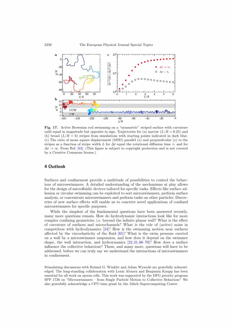
be taken one step further by using structured walls [63]. By using striped surfaces,for which neighboring stripes induce an opposite sense of circular motion, bacteriacan be made to follow stripe boundaries in a snaking-like motion, as they are alwaysdirected back to the stripe boundary by the alternating CW and CCW motions. Ofcourse, this snaking motion is only possible if the stripe width L is large enough thatthe bacterium does not hit a second stripe boundary before being able to return tothe first. Therefore, in the case that L is smaller than the circle radius R, the bacterialmotion is hardly affected by the surface structure. This is illustrated in Fig. 17a,b.As a results, the diffusional motion depends strongly on the ratio L/R, and becomeshighly anisotropic for L/R > 1, as shown in Fig. 17c. Striped surfaces can thereforebe employed to separate bacteria with different trajectory radii!


Fig. 17. Active Brownian rod swimming on a “symmetric” striped surface with curvatureradii equal in magnitude but opposite in sign. Trajectories for (a) narrow (L/R = 0.25) and(b) broad (L/R = 6) stripes from simulations with starting points indicated in dark blue.(c) The ratio of mean square displacement (MSD) parallel (x) and perpendicular (y) to thestripes as a function of stripe width L for Δt equal the rotational diffusion time τr and forΔt → ∞. From Ref. [63]. (This figure is subject to copyright protection and is not coveredby a Creative Commons license.)

4 Outlook

Surfaces and confinement provide a multitude of possibilities to control the behav-iour of microswimmers. A detailed understanding of the mechanisms at play allowsfor the design of microfluidic devices tailored for specific tasks. Effects like surface ad-hesion or circular swimming can be exploited to sort microswimmers, perform surfaceanalysis, or concentrate microswimmers and perform tasks on other particles. Discov-eries of new surface effects will enable us to conceive novel applications of confinedmicroswimmers for specific purposes.

While the simplest of the fundamental questions have been answered recently,many more questions remain. How do hydrodynamic interactions look like for morecomplex confining geometries, i.e. beyond the infinite planar wall? What is the effectof curvature of surfaces and microchannels? What is the role of (active) noise incompetition with hydrodynamics [24]? How is the swimming motion near surfacesaffected by the viscoelasticity of the fluid [65]? What is the swim pressure exertedon a wall by a microswimmer suspension, and how does it depend on the swimmershape, the wall interaction, and hydroynamics [22,31,66–70]? How does a surfaceinfluence the collective behaviour? These, and many more, questions will have to beaddressed, before we can truly say we understand the interactions of microswimmersin confinement.

Stimulating discussions with Roland G. Winkler and Adam Wysocki are gratefully acknowl-edged. The long-standing collaboration with Louis Alvarez and Benjamin Kaupp has beenessential for all work on sperm cells. This work was supported by the DFG priority programSPP 1726 on “Microswimmers – from Single Particle Motion to Collective Behaviour” Wealso gratefully acknowledge a CPU-time grant by the Julich Supercomputing Center.


References

1. L. Rothschild, Nature 198, 1221 (1963)2. B.M. Friedrich, I.H. Riedel-Kruse, J. Howard, F. Julicher, J. Exp. Biol. 213, 1226 (2010)3. W.R. DiLuzio, L. Turner, M. Mayer, P. Garstecki, D.B. Weibel, H.C. Berg, G.M.Whitesides, Nature 435, 1271 (2005)

4. E. Lauga, W.R. DiLuzio, G.M. Whitesides, H.A. Stone, Biophys. J. 90, 400 (2006)5. J. Elgeti, R.G. Winkler, G. Gompper, Rep. Prog. Phys. 78, 056601 (2015)6. G.A. Ozin, I. Manners, S. Fournier-Bidoz, A. Arsenault, Adv. Mater. 17, 3011 (2005)7. S. Sengupta, M.E. Ibele, A. Sen, Angew. Chem. Int. Ed. 51, 8434 (2012)8. G. Gompper, Spektrum der Wissenschaft Heft 4, 84 (2015)9. H.P. Zhang, A. Be’er, E.-L. Florin, H.L. Swinney, Proc. Natl. Acad. Sci. USA 107, 13626(2010)

10. S.E. Hulme, W.R. DiLuzio, S.S. Shevkoplyas, L. Turner, M. Mayer, H.C. Berg, G.M.Whitesides, Lab Chip 8, 1888 (2008)

11. P. Denissenko, V. Kantsler, D.J. Smith, J. Kirkman-Brown, Proc. Natl. Acad. Sci. USA109, 8007 (2012)

12. M.C. Marchetti, Y. Fily, S. Henkes, A. Patch, D. Yllanes, Curr. Opin. Colloid InterfaceSci. 21, 34 (2016)

13. T. Speck, Eur. Phys. J. Special Topics 225, 2287 (2016)14. F. Peruani, Eur. Phys. J. Special Topics 225, 3001 (2016)15. J. Elgeti, G. Gompper, EPL 85, 38002 (2009)16. G. Li, J.X. Tang, Phys. Rev. Lett. 103, 078101 (2009)17. A.C. Maggs, D.A. Huse, S. Leibler, Europhys. Lett. 8, 615 (1989)18. T.W. Burkhardt, J. Stat. Mech. p. P07004 (2007)19. H.H. Wensink H. Lowen, Phys. Rev. E 78, 031409 (2008)20. J. Elgeti, R.G. Winkler, G. Gompper, SoftComp Newsletter 12, (2015), http://www.eu-softcomp.net.

21. J. Elgeti G. Gompper, EPL 101, 48003 (2013)22. A. Wysocki, J. Elgeti, G. Gompper, Phys. Rev. E 91, 050302(R) (2015)23. S.E. Spagnolie, G.R. Moreno-Flores, D. Bartolo, E. Lauga, Soft Matter 11, 3396 (2015)24. K. Schaar, A. Zottl, H. Stark, Phys. Rev. Lett. 115, 038101 (2015)25. Y. Fily, A. Baskaran, M.F. Hagan, Soft Matter 10, 5609 (2014)26. J. Elgeti, G. Gompper, EPL 109, 58003 (2015)27. H.C. Berg, E. coli in Motion (Springer, New York, 2004)28. J. Tailleur, M.E. Cates, EPL 86, 60002 (2009)29. M.E. Cates, J. Tailleur, EPL 101, 20010 (2013)30. A.P. Solon, M.E. Cates, J. Tailleur, Eur. Phys. J. Special Topics 224, 1231 (2015)31. B. Ezhilan, R. Alonso-Matilla, D. Saintillan, J. Fluid Mech. 781, R4 (2015)32. H.C. Berg, D.A. Brown, Nature 239, 500 (1972)33. M. Molaei, M. Barry, R. Stocker, J. Sheng, Phys. Rev. Lett. 113, 068103 (2014)34. E. Lauga, T.R. Powers, Rep. Prog. Phys. 72, 096601 (2009)35. T. Ishikawa, J.R. Soc. Interface 6, 815 (2009)36. R.G. Winkler, Eur. Phys. J. Special Topics 225, 2079 (2016)37. K. Drescher, J. Dunkel, L.H. Cisneros, S. Ganguly, R.E. Goldstein, Proc. Natl. Acad.Sci. USA 108, 10940 (2011)

38. U.B. Kaupp, L. Alvarez, Eur. Phys. J. Special Topics 225, 2119 (2016)39. R. Jeanneret, M. Contino, M. Polin, Eur. Phys. J. Special Topics 225, 2141 (2016)40. A.P. Berke, L. Turner, H.C. Berg, E. Lauga, Phys. Rev. Lett. 101, 038102 (2008)41. D. Takagi, J. Palacci, A.B. Braunschweig, M.J. Shelley, J. Zhang, Soft Matter 10, 1784(2014)

42. I.O. Gotze G. Gompper, Phys. Rev. E 82, 041921 (2010)43. T. Ishikawa, M.P. Simmonds, T.J. Pedley, J. Fluid Mech. 568, 119 (2006)44. K. Ishimoto, E.A. Gaffney, Phys. Rev. E 88, 062702 (2013)45. G.-J. Li, A.M. Ardekani, Phys. Rev. E 90, 013010 (2014)46. J. Elgeti, U.B. Kaupp, G. Gompper, Biophys. J. 99, 1018 (2010)


47. B.M. Friedrich, F. Julicher, New J. Phys. 10, 123025 (2008)48. B.M. Friedrich, F. Julicher, Phys. Rev. Lett. 103, 068102 (2009)49. I.H. Riedel, K. Kruse, J. Howard, Science 309, 300 (2005)50. Y. Yang, F. Qiu, G. Gompper, Phys. Rev. E 89, 012720 (2014)51. K. Miki D.E. Clapham, Curr. Biol. 18, 443 (2013)52. V. Kantsler, J. Dunkel, M. Blayney, R.E. Goldstein, eLife 3, e02403 (2014)53. K. Ishimoto, E.A. Gaffney, J. Roy. Soc. Interface 12, 20150172 (2015)54. H. Lowen, Eur. Phys. J. Special Topics 225, 3019 (2016)55. H. Stark, Eur. Phys. J. Special Topics 225, 3069 (2016)56. L. Lemelle, J.-F. Palierne,E. Chatre, C. Vaillant, C. Place, Soft Matter 9, 9759 (2013)57. L. Lemelle, J. Palierne, E. Chatre, C. Place, J. Bacteriol. 192, 6307 (2010)58. R. Di Leonardo, D. Dell’Arciprete, L. Angelani, V. Iebba, Phys. Rev. Lett. 106, 038101(2011)

59. K.M. Ottemann, J.F. Miller, Mol. Microbiol. 24, 1109 (1997)60. L.A. Pratt, R.R. Kolter, Mol. Microbiol. 30, 285 (1998)61. Podcast “Welt der Physik, Folge 189 – Mikroschwimmer im Modell” (09. Juli 2015);http://www.weltderphysik.de/mediathek/podcast/.

62. I.O. Gotze, G. Gompper, EPL 92, 64003 (2010)63. J. Hu, A. Wysocki, R.G. Winkler, G. Gompper, Sci. Rep. 5, 9586 (2015)64. J. Hu, M. Yang, G. Gompper, R.G. Winkler, Soft Matter 11, 7867 (2015)65. G.-J. Li, A. Karimi, A.M. Ardekani, Rheol. Acta 53, 911 (2014)66. X. Yang, M.L. Manning, M.C. Marchetti, Soft Matter 10, 6477 (2014)67. S.C. Takatori, W. Yan, J.F. Brady, Phys. Rev.Lett. 113, 028103 (2014)68. A.P. Solon, J. Stenhammar, R. Wittkowski, M. Kardar, Y. Kafri, M.E. Cates, J. Tailleur,Phys. Rev. Lett. 114, 198301 (2015)

69. A.P. Solon, Y. Fily, A. Baskaran, M.E. Cates, Y. Kafri, M. Kardar, J. Tailleur, Nat.Phys. 11, 673 (2015)

70. R.G. Winkler, A. Wysocki, G. Gompper, Soft Matter 11, 6680 (2015)

Open Access This is an Open Access article distributed under the terms of theCreative Commons Attribution License (http://creativecommons.org/licenses/by/4.0),which permits unrestricted use, distribution, and reproduction in any medium,provided the original work is properly cited.

microswimmers near surfaces - springer · 2336 theeuropeanphysicaljournalspecialtopics fig. 3....

Documents