microwave radar cross sections and doppler velocities ... · pdf filemicrowave radar cross...

Microwave radar cross sections and Doppler

velocities measured in the surf zone

Gordon Farquharson1 and Stephen J. FrasierMicrowave Remote Sensing Laboratory, University of Massachusetts, Amherst, Massachusetts, USA

Britt Raubenheimer and Steve ElgarWoods Hole Oceanographic Institution, Woods Hole, Massachusetts, USA

Received 23 April 2005; revised 26 July 2005; accepted 14 September 2005; published 23 December 2005.

[1] The relationship between microwave imaging radar measurements of fluid velocitiesin the surf zone and shoaling, breaking, and broken waves is studied with fieldobservations. Normalized radar cross section (NRCS) and Doppler velocity are estimatedfrom microwave measurements at near-grazing angles, and in situ fluid velocities aremeasured with acoustic Doppler velocimeters (ADVs). Joint histograms of radar crosssection and Doppler velocity cluster into identifiable distributions. The NRCS values frompixels with large NRCS and high Doppler velocities (>2 m/s) decrease with decreasingbore height to the shoreline, similar to scattering from a cylinder with decreasing radius.The Doppler velocities associated with these regions in the histograms agree well withtheoretical wave phase velocities. Radar and ADV measurements of fluid velocitiesbetween bore crests have similarly shaped energy density spectra for frequencies aboveabout 0.1 Hz, but energy levels from the radar are an order of magnitude higher than thoseof the ADV data. Instantaneous interbore Doppler velocities are correlated with ADVmeasured fluid velocities but are offset by 0.8 m/s. This offset may be due to Bragg wavephase velocities, wind drift, range and azimuth sidelobes, the finite spatial resolution of theradar, and differences between mean flows measured at the surface with radar andflows measured below the surface with ADVs. Shoaling and breaking waves measuredthrough radar grating lobes significantly affect both the Doppler velocities near the edgesof the images and the scattering from the rear faces of waves, causing large Dopplervelocities to be observed in these regions.

Citation: Farquharson, G., S. J. Frasier, B. Raubenheimer, and S. Elgar (2005), Microwave radar cross sections and Doppler

velocities measured in the surf zone, J. Geophys. Res., 110, C12024, doi:10.1029/2005JC003022.

1. Introduction

[2] Measurement of nearshore processes traditionally isaccomplished using fixed or drifting in situ devices. Pres-sure sensors are used to derive wave height, and electro-magnetic current meters and acoustic Doppler velocimeters(ADVs) are used to measure subsurface velocity. However,large spatial coverage with sensor spacing fine enough toensure measurement of small-scale nearshore processes,such as rip currents, leads to a prohibitively large numberof in situ devices. Also, the deployment of these sensorstends to be difficult and time-consuming, and constantmaintenance is required to remove debris, such as kelp, thatcollects on instrument mounting frames. Furthermore,sensors occasionally are buried as the bathymetry changes,contributing to the difficulties of long-term deployment. In

situ sensors are also a hazard to swimmers and surfers, andinjuries have occurred despite sufficient warning of instru-ment placement during experiments. To overcome some ofthese problems, other types of in situ instruments are used,such as drifters, which provide larger-scale Lagrangianmeasurements of currents. However, drifters require labor-intensive deployment and retrieval. Consequently, remotesensing techniques have been investigated as a means toprovide large-scale measurements of nearshore processes.[3] Optical, acoustic, and radar-based remote sensing

techniques have been used to measure nearshore processes.Optical techniques have been used to provide estimates ofthe time-varying sandbar position [Lippmann and Holman,1990], alongshore currents in the surf zone [Chickadel etal., 2003], statistics of swash zone run-up [Holman andGuza, 1984; Holman and Sallenger, 1985; Holland andHolman, 1993], and bathymetry [Dugan et al., 2001].Processing of video images, such as tracking surface foamusing particle image velocimetry derived algorithms, typi-cally relies on visual contrast in the image, thus generallyrestricting optical techniques to the surf zone duringdaylight.

JOURNAL OF GEOPHYSICAL RESEARCH, VOL. 110, C12024, doi:10.1029/2005JC003022, 2005

1Now at Earth Observing Laboratory, National Center for AtmosphericResearch, Boulder, Colorado, USA.

Copyright 2005 by the American Geophysical Union.0148-0227/05/2005JC003022$09.00

C12024 1 of 12

[4] Doppler sonar has been used in the nearshore tomeasure acoustic intensity and Doppler velocities in ripcurrents [Smith, 1993; Smith and Largier, 1995]. Theacoustic intensity is proportional to a combination of bubbledensity and suspended sediment, and Doppler velocity is theline of sight (radial) component of the scatterer velocity.However, acoustic measurements are limited by attenuationdue to high densities of subsurface bubbles generated bybreaking waves within the surf zone. Thus development ofother techniques to measure velocities both inside andoffshore of the surf zone is desirable.[5] Microwave radar has proven to be useful in mea-

suring oceanographic parameters, such as directionalwave spectra [Young et al., 1985; Frasier et al., 1995],surface currents [McGregor et al., 1997; Moller et al.,1998], and nearshore bathymetric changes [McGregor etal., 1998; Trizna, 2001]. However, radar has not beenextensively applied to measuring surf zone currents. Inthis region, shoaling and breaking waves complicate theinterpretation of Doppler velocities because different scat-tering mechanisms govern radar echos from broken andunbroken water surfaces. That is, Doppler velocitiesreflect the locally dominant scattering mechanism. Thispaper addresses the interpretation of microwave scatteringwithin the surf zone.[6] Microwave radar estimates of surf zone velocities

have been compared with video-based estimates [Puleo etal., 2003]. The results presented here extend previousstudies by comparing radar with in situ current meters,allowing the radar to be ground truthed and, by investi-gating radar returns in more detail, allowing backscatter-ing from shoreward propagating bores to be separatedfrom backscattering from the water surface betweenbores.[7] This paper starts with a brief overview of micro-

wave radar scattering from the ocean surface in section 2.The field experiment and data collection are described insection 3, and the radar data processing is described insection 4. Estimates of normalized radar cross section(NRCS) and radar Doppler velocities and comparisonswith in situ ADV-measured fluid velocities are presentedin section 5. Radar image statistics are derived and usedto characterize surf zone scattering. Doppler velocitiesassociated with large NRCS features are compared withbore phase velocities, and interbore Doppler velocities arecompared with in situ fluid velocities. Conclusions arepresented in section 6.

2. Microwave Radar Scattering

[8] For vertical polarization at moderate incidence angles(20�–70�) and no wave breaking, microwave radar scatter-ing from the ocean surface commonly is described by two-scale scattering from tilted, ‘‘slightly rough’’ surfaces[Wright, 1968; Valenzuela, 1968]. At X band frequencies,wind-generated gravity-capillary waves produce a slightlyrough water surface. Larger-scale gravity waves are treatedby dividing the surface into tilted facets that are locallyslightly rough. In this formalism the radar cross section isdetermined primarily by the surface displacement spectrumevaluated at the Bragg resonant wavelength (approximately1.5 cm for X band radar at near-grazing incidence angles).

The Doppler velocity measured by the radar is the power-weighted mean of the phase velocity of both the advancingand receding Bragg resonant waves (vb) in a resolution cellplus any advection of the facet due to gravity wave orbitalvelocities (vo), surface currents (vc), and wind drift (vw)[Plant, 1990].[9] Composite surface theory and two-scale models do

not describe the observed scattering from breaking waveson the ocean surface. Backscatter from breaking waves isobserved to have large radar cross section values andDoppler velocities on the order of a few m/s [Lewis andOlin, 1980; Keller et al., 1986; Lee et al., 1995; Liu et al.,1998; Frasier et al., 1998]. Recent radar measurements ofthe surf zone region show significant backscatter for steep-ening waves, as well as for breaking waves and brokenwhite water bores [Puleo et al., 2003; Haller and Lyzenga,2003]. Thus, for breaking waves, it is known that non-Bragg scattering mechanisms dominate over Bragg scatter-ing at low grazing angles and that multiple scattering andmultipath interference become increasingly important withincreasing wave steepness and surface roughness [Lee et al.,1999].[10] Recent laboratory and field studies of scattering from

breaking waves [e.g., Sletten et al., 2003; Puleo et al., 2003]confirm that observed Doppler velocities are consistent withthe phase velocities of breaking waves. Thus radar crosssections for breaking waves in the surf zone are expected tobe large compared with those for deep water nonbreakingwaves, and surf zone Doppler velocities are expected to beon the order of wave phase velocities.[11] The nearshore contains a variety of phenomena,

including actively breaking waves in the breaker zone,white water bores in the surf zone, and unbroken watersurfaces between wave crests, and thus a complex relation-ship exists between microwave backscatter and nearshoreprocesses. This relationship is explored here by character-izing microwave scattering in the nearshore and relating themeasurements to nearshore waves and fluid velocities.

3. Field Experiment

[12] Vertically polarized backscattered power and Dopp-ler velocities were measured in the nearshore region atScripps Beach, La Jolla, California [Puleo et al., 2003]from 1700 to 1800 UT on 10 October 2000 using a second-generation Focused Phased Array Imaging Radar (FOPAIR)[McIntosh et al., 1995]. FOPAIR is an X band microwaveDoppler radar designed to image the sea surface with meter-scale resolution. The radar was deployed on the roof of abuilding 13.52 m above mean sea level (Figure 1). Theimaging footprint of the radar system covered a 30� azi-muthal sector with a resolution of 0.5� and a 384 m rangewith a resolution of 3 m. Radar images were recorded at arate of 2.2 Hz over 20 min data runs.[13] Simultaneously, a cross-shore transect of acoustic

Doppler velocimeters and pressure sensors (Figure 1, dia-monds) was used to measure subsurface fluid velocities andwave heights [Raubenheimer, 2002]. Data from the ADVswere recorded at 16 Hz for 3072 s (51.2 min) starting everyhour. The distance from downward looking ADVs (locatedat cross-shore positions x = 185, 144, 116, 66, and 56 m,Figure 1) to the seabed was measured every 3 s for 6.4 min

C12024 FARQUHARSON ET AL.: RADAR MEASUREMENTS IN THE SURF ZONE

2 of 12

C12024

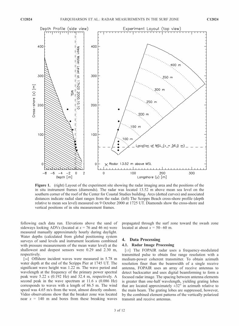
following each data run. Elevations above the sand ofsideways looking ADVs (located at x = 76 and 46 m) weremeasured manually approximately hourly during daylight.Water depths (calculated from global positioning systemsurveys of sand levels and instrument locations combinedwith pressure measurements of the mean water level) at theshallowest and deepest sensors were 0.29 and 2.30 m,respectively.[14] Offshore incident waves were measured in 5.78 m

water depth at the end of the Scripps Pier at 1745 UT. Thesignificant wave height was 1.22 m. The wave period andwavelength at the frequency of the primary power spectralpeak were 5.22 s (0.192 Hz) and 32.4 m, respectively. Asecond peak in the wave spectrum at 11.6 s (0.086 Hz)corresponds to waves with a length of 86.5 m. The windspeed was 4.65 m/s from the west, almost directly onshore.Video observations show that the breaker zone was locatednear x = 140 m and bores from these breaking waves

propagated through the surf zone toward the swash zonelocated at about x = 50–60 m.

4. Data Processing

4.1. Radar Image Processing

[15] The FOPAIR radar uses a frequency-modulatedtransmitted pulse to obtain fine range resolution with amedium-power coherent transmitter. To obtain azimuthresolution finer than the beamwidth of a single receiveantenna, FOPAIR uses an array of receive antennas todetect backscatter and uses digital beamforming to form afocused radar image. The spacing between antenna elementsis greater than one-half wavelength, yielding grating lobesthat are located approximately ±32� in azimuth relative tothe main beam. The grating lobes are suppressed, however,by the combined element patterns of the vertically polarizedtransmit and receive antennas.

Figure 1. (right) Layout of the experiment site showing the radar imaging area and the positions of thein situ instrument frames (diamonds). The radar was located 13.52 m above mean sea level on thesouthern corner of the roof of the Center for Coastal Studies building. Arcs (dotted curves) and associateddistances indicate radial slant ranges from the radar. (left) The Scripps Beach cross-shore profile (depthrelative to mean sea level) measured on 9 October 2000 at 1725 UT. Diamonds show the cross-shore andvertical positions of in situ measurement frames.


3 of 12

C12024

[16] The radar forms an image of the ocean surface in aperiod of approximately 0.64 ms, which is well within thedecorrelation time for microwave backscatter at X band[Plant et al., 1994]. A subsequent image is captured at t =1.5 ms later, and the covariance of the images R(t) iscomputed for each pixel. The phase of R(t) divided by2pt has been shown to be an unbiased estimator of the firstmoment of the Doppler spectrum [Miller and Rochwarger,1972], and thus

�vD ¼ �l2

arg R tð Þf g2pt

ð1Þ

is an estimate of the mean Doppler velocity, where l is theradar wavelength.[17] Backscattered power and velocity are time averaged

to produce a processed data image rate of 2.2 Hz. For apulse pair spacing of 1.5 ms the unambiguous Dopplervelocity range is ±5 m/s. Doppler velocities from advancingbreaking waves occasionally exceed the maximum unam-biguous velocity. For this work, these velocities are unwrap-ped by adding observed (aliased) velocity values less than�2 to 10 m/s. NRCS (s0) values are estimated from meanbackscattered power measurements using nominal systemparameters.[18] For each pixel in the radar image the minimum radar

cross section is estimated from the measured noise figure ofthe receiver and an assumed operating temperature. Theminimum NRCS detectable by the radar along the centerbeam ranges from below �50 dB along the boresightdirection for near ranges to �36 dB at far ranges. At theedges of the image, sensitivity decreases and the minimumNRCS is between �40 and �20 dB. Typical NRCS valuesmeasured at grazing angles of around 1� with low tomoderate wind speeds are around �40 dB [Wetzel, 1990].Thus it is expected that near the edges of the images, pixelswill contain NRCS values that are less than the minimumdetectable NRCS. The processing code marks such pixels asmissing data.

4.2. Radar and in Situ Time Series Processing

[19] To compare radar with ADV time series, radartime series were interpolated to the 16 Hz sampling rateof the ADVs. Both time series were then low�passfiltered with a cutoff frequency of 1 Hz and decimatedto a sampling rate of 2 Hz. This procedure ensures thatthe filter has the same effect on both Doppler and currentmeter time series.[20] Subsurface velocities (vhs

i ) are converted to surfacevelocities (v0

i ) using linear wave theory [Guza andThornton, 1980] in which

vi0 ¼cosh khð Þ

cosh k h� hsð Þð Þ vihs; ð2Þ

where k is the wave number of the ocean waves, h is thewater depth, hs is the distance above the bottom of thesubsurface sensor, and the superscript i indicates the cross-shore and alongshore components of horizontal velocity.The correction was applied at wind wave frequencies(0.005 Hz � f � 0.300 Hz) for all the in situ velocitiespresented here.

[21] The radial component of the surface velocity iscomputed using

vradial ¼ u0 sin fð Þ � v0 cos fð Þ; ð3Þ

where u0 is the cross-shore velocity, v0 is the alongshorevelocity, and f is the angle from the radar to the sensormeasured from the positive alongshore direction.

5. Results and Analysis

5.1. Radar Images

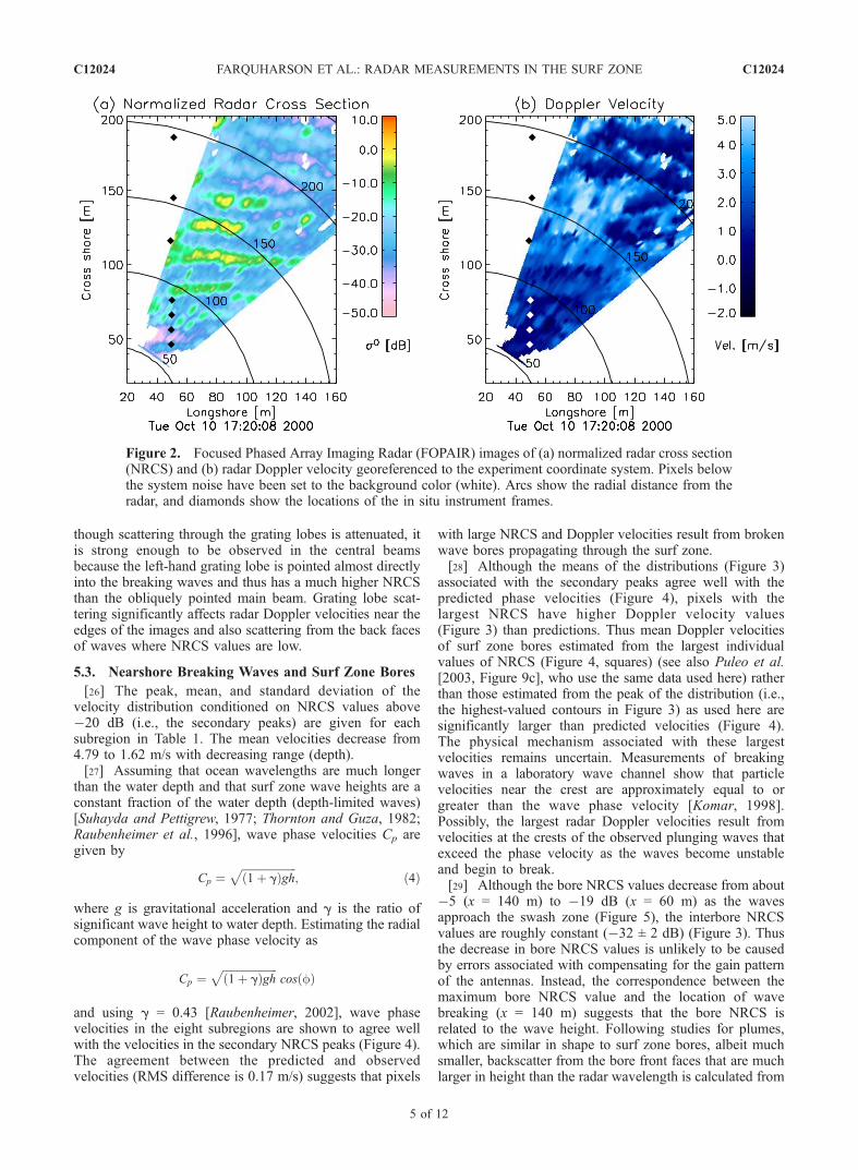
[22] Images of normalized radar cross section and asso-ciated Doppler velocity georeferenced to the experimentcoordinate system (Figure 2) show that NRCS (s0) valuesrange from �50 to around 0 dB. NRCS signatures ofbreaking wave crests in the surf zone (70 m � x � 140 m)are above �10 dB and are mostly parallel to the shore.NRCS values between these bright features are around�30 dB. Some evidence of backscattered power measuredthrough grating lobes is seen on the left-hand side of theimage at x = 110–130, 160, and 200 m, where scatteringfrom bright features appears to wrap around from the right-hand side of the image and to continue on the left at thesame radial range.[23] Unwrapped radar Doppler velocities range from �2

to 5 m/s. Positive Doppler velocities represent motiontoward the radar. Individual Doppler velocity wave signa-tures, especially between radial ranges from 120 to 170 m,are less distinct than those in the NRCS image.

5.2. NRCS and Doppler Velocity Distributions

[24] Breaking wave fronts result in large radar crosssections (Figure 2, yellow bands), with Doppler velocitieson the order of the phase velocity of the wave. In contrast,interbore radar cross sections (Figure 2, blue areas) are moresimilar to offshore NRCS values, suggesting Bragg-dominated scattering in which Doppler velocities are acombination of water particle orbital velocity, Bragg wavephase velocity, and surface currents. Each of these processescan be identified by its distinct distribution of NRCS andradar Doppler velocities.[25] To mitigate the effect of grating lobes, which affect

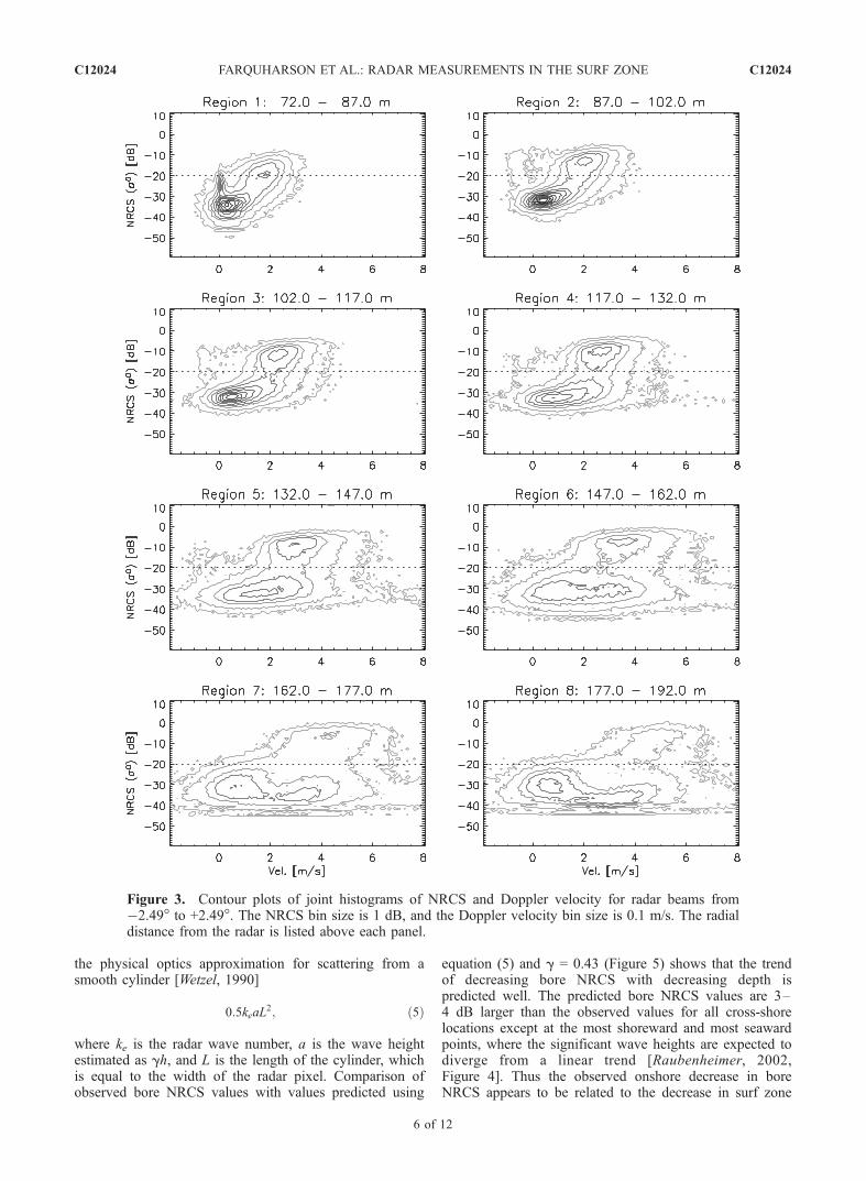
Doppler velocities near the edges of the radar images, jointhistograms of NRCS and Doppler velocities (Figure 3) werecomputed using only the central radar beams between�2.49� and +2.49� and between radial ranges from 72 to192 m. For these beam angles the grating lobe suppressionis greater than 43 dB. All regions show peaks in thehistograms at s0 near �30 dB and velocities near 0.5 m/s.A secondary peak with s0 > �20 dB and velocity >2 m/salso exists for all regions. The sources of these peaks will bediscussed in sections 5.3 and 5.4. The near-zero velocitypeak in region 1 is due to scattering from the stationaryinstrument frames on which the in situ sensors weremounted. In regions 5–8, another peak occurs at s0 <�30 dB and velocity >2 m/s. Backscatter in this distributionis due to scattering from shoaling and breaking wavesmeasured through the radar grating lobes, and thus NRCSvalues in this distribution are not representative of the trueNRCS because they are converted from backscatteredpower to NRCS using the main beam antenna gain. Al-


4 of 12

C12024

though scattering through the grating lobes is attenuated, itis strong enough to be observed in the central beamsbecause the left-hand grating lobe is pointed almost directlyinto the breaking waves and thus has a much higher NRCSthan the obliquely pointed main beam. Grating lobe scat-tering significantly affects radar Doppler velocities near theedges of the images and also scattering from the back facesof waves where NRCS values are low.

5.3. Nearshore Breaking Waves and Surf Zone Bores

[26] The peak, mean, and standard deviation of thevelocity distribution conditioned on NRCS values above�20 dB (i.e., the secondary peaks) are given for eachsubregion in Table 1. The mean velocities decrease from4.79 to 1.62 m/s with decreasing range (depth).[27] Assuming that ocean wavelengths are much longer

than the water depth and that surf zone wave heights are aconstant fraction of the water depth (depth-limited waves)[Suhayda and Pettigrew, 1977; Thornton and Guza, 1982;Raubenheimer et al., 1996], wave phase velocities Cp aregiven by

Cp ¼ffiffiffiffiffiffiffiffiffiffiffiffiffiffiffiffiffiffiffiffi1þ gð Þgh

p; ð4Þ

where g is gravitational acceleration and g is the ratio ofsignificant wave height to water depth. Estimating the radialcomponent of the wave phase velocity as

Cp ¼ffiffiffiffiffiffiffiffiffiffiffiffiffiffiffiffiffiffiffiffi1þ gð Þgh

pcosðfÞ

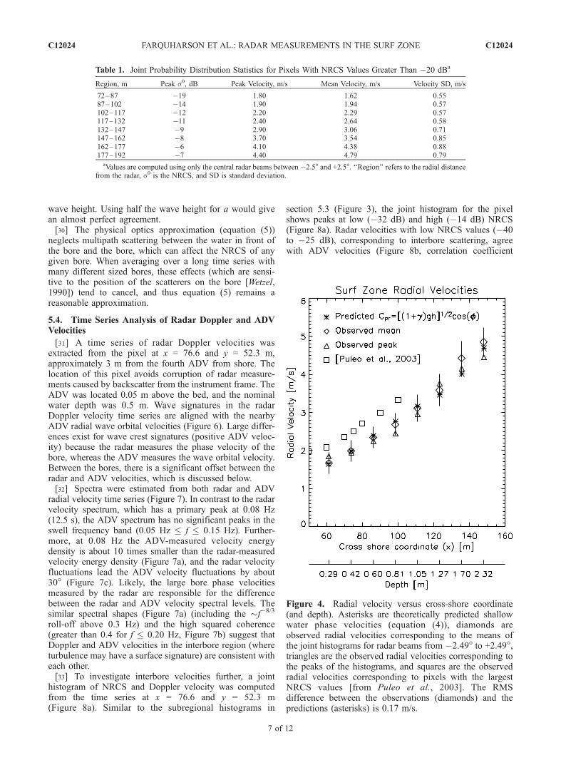
and using g = 0.43 [Raubenheimer, 2002], wave phasevelocities in the eight subregions are shown to agree wellwith the velocities in the secondary NRCS peaks (Figure 4).The agreement between the predicted and observedvelocities (RMS difference is 0.17 m/s) suggests that pixels

with large NRCS and Doppler velocities result from brokenwave bores propagating through the surf zone.[28] Although the means of the distributions (Figure 3)

associated with the secondary peaks agree well with thepredicted phase velocities (Figure 4), pixels with thelargest NRCS have higher Doppler velocity values(Figure 3) than predictions. Thus mean Doppler velocitiesof surf zone bores estimated from the largest individualvalues of NRCS (Figure 4, squares) (see also Puleo et al.[2003, Figure 9c], who use the same data used here) ratherthan those estimated from the peak of the distribution (i.e.,the highest-valued contours in Figure 3) as used here aresignificantly larger than predicted velocities (Figure 4).The physical mechanism associated with these largestvelocities remains uncertain. Measurements of breakingwaves in a laboratory wave channel show that particlevelocities near the crest are approximately equal to orgreater than the wave phase velocity [Komar, 1998].Possibly, the largest radar Doppler velocities result fromvelocities at the crests of the observed plunging waves thatexceed the phase velocity as the waves become unstableand begin to break.[29] Although the bore NRCS values decrease from about

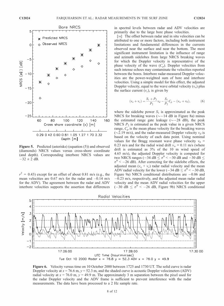
�5 (x = 140 m) to �19 dB (x = 60 m) as the wavesapproach the swash zone (Figure 5), the interbore NRCSvalues are roughly constant (�32 ± 2 dB) (Figure 3). Thusthe decrease in bore NRCS values is unlikely to be causedby errors associated with compensating for the gain patternof the antennas. Instead, the correspondence between themaximum bore NRCS value and the location of wavebreaking (x = 140 m) suggests that the bore NRCS isrelated to the wave height. Following studies for plumes,which are similar in shape to surf zone bores, albeit muchsmaller, backscatter from the bore front faces that are muchlarger in height than the radar wavelength is calculated from

Figure 2. Focused Phased Array Imaging Radar (FOPAIR) images of (a) normalized radar cross section(NRCS) and (b) radar Doppler velocity georeferenced to the experiment coordinate system. Pixels belowthe system noise have been set to the background color (white). Arcs show the radial distance from theradar, and diamonds show the locations of the in situ instrument frames.


5 of 12

C12024

the physical optics approximation for scattering from asmooth cylinder [Wetzel, 1990]

0:5keaL2; ð5Þ

where ke is the radar wave number, a is the wave heightestimated as gh, and L is the length of the cylinder, whichis equal to the width of the radar pixel. Comparison ofobserved bore NRCS values with values predicted using

equation (5) and g = 0.43 (Figure 5) shows that the trendof decreasing bore NRCS with decreasing depth ispredicted well. The predicted bore NRCS values are 3–4 dB larger than the observed values for all cross-shorelocations except at the most shoreward and most seawardpoints, where the significant wave heights are expected todiverge from a linear trend [Raubenheimer, 2002,Figure 4]. Thus the observed onshore decrease in boreNRCS appears to be related to the decrease in surf zone

Figure 3. Contour plots of joint histograms of NRCS and Doppler velocity for radar beams from�2.49� to +2.49�. The NRCS bin size is 1 dB, and the Doppler velocity bin size is 0.1 m/s. The radialdistance from the radar is listed above each panel.


6 of 12

C12024

wave height. Using half the wave height for a would givean almost perfect agreement.[30] The physical optics approximation (equation (5))

neglects multipath scattering between the water in front ofthe bore and the bore, which can affect the NRCS of anygiven bore. When averaging over a long time series withmany different sized bores, these effects (which are sensi-tive to the position of the scatterers on the bore [Wetzel,1990]) tend to cancel, and thus equation (5) remains areasonable approximation.

5.4. Time Series Analysis of Radar Doppler and ADVVelocities

[31] A time series of radar Doppler velocities wasextracted from the pixel at x = 76.6 and y = 52.3 m,approximately 3 m from the fourth ADV from shore. Thelocation of this pixel avoids corruption of radar measure-ments caused by backscatter from the instrument frame. TheADV was located 0.05 m above the bed, and the nominalwater depth was 0.5 m. Wave signatures in the radarDoppler velocity time series are aligned with the nearbyADV radial wave orbital velocities (Figure 6). Large differ-ences exist for wave crest signatures (positive ADV veloc-ity) because the radar measures the phase velocity of thebore, whereas the ADV measures the wave orbital velocity.Between the bores, there is a significant offset between theradar and ADV velocities, which is discussed below.[32] Spectra were estimated from both radar and ADV

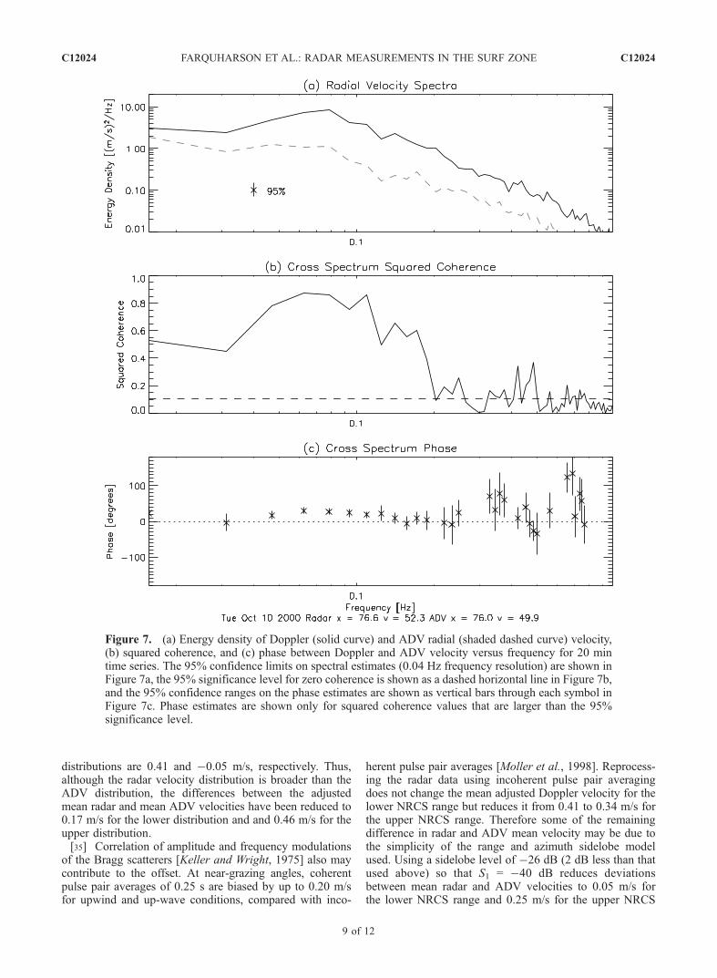
radial velocity time series (Figure 7). In contrast to the radarvelocity spectrum, which has a primary peak at 0.08 Hz(12.5 s), the ADV spectrum has no significant peaks in theswell frequency band (0.05 Hz � f � 0.15 Hz). Further-more, at 0.08 Hz the ADV-measured velocity energydensity is about 10 times smaller than the radar-measuredvelocity energy density (Figure 7a), and the radar velocityfluctuations lead the ADV velocity fluctuations by about30� (Figure 7c). Likely, the large bore phase velocitiesmeasured by the radar are responsible for the differencebetween the radar and ADV velocity spectral levels. Thesimilar spectral shapes (Figure 7a) (including the f�8/3

roll-off above 0.3 Hz) and the high squared coherence(greater than 0.4 for f � 0.20 Hz, Figure 7b) suggest thatDoppler and ADV velocities in the interbore region (whereturbulence may have a surface signature) are consistent witheach other.[33] To investigate interbore velocities further, a joint

histogram of NRCS and Doppler velocity was computedfrom the time series at x = 76.6 and y = 52.3 m(Figure 8a). Similar to the subregional histograms in

section 5.3 (Figure 3), the joint histogram for the pixelshows peaks at low (�32 dB) and high (�14 dB) NRCS(Figure 8a). Radar velocities with low NRCS values (�40to �25 dB), corresponding to interbore scattering, agreewith ADV velocities (Figure 8b, correlation coefficient

Table 1. Joint Probability Distribution Statistics for Pixels With NRCS Values Greater Than �20 dBa

Region, m Peak s0, dB Peak Velocity, m/s Mean Velocity, m/s Velocity SD, m/s

72–87 �19 1.80 1.62 0.5587–102 �14 1.90 1.94 0.57102–117 �12 2.20 2.29 0.57117–132 �11 2.40 2.64 0.58132–147 �9 2.90 3.06 0.71147–162 �8 3.70 3.54 0.85162–177 �6 4.10 4.38 0.88177–192 �7 4.40 4.79 0.79

aValues are computed using only the central radar beams between �2.5� and +2.5�. ‘‘Region’’ refers to the radial distancefrom the radar, s0 is the NRCS, and SD is standard deviation.

Figure 4. Radial velocity versus cross-shore coordinate(and depth). Asterisks are theoretically predicted shallowwater phase velocities (equation (4)), diamonds areobserved radial velocities corresponding to the means ofthe joint histograms for radar beams from �2.49� to +2.49�,triangles are the observed radial velocities corresponding tothe peaks of the histograms, and squares are the observedradial velocities corresponding to pixels with the largestNRCS values [from Puleo et al., 2003]. The RMSdifference between the observations (diamonds) and thepredictions (asterisks) is 0.17 m/s.


7 of 12

C12024

r2 = 0.43) except for an offset of about 0.81 m/s (e.g., themean velocities are 0.67 m/s for the radar and –0.14 m/sfor the ADV). The agreement between the radar and ADVinterbore velocities supports the assertion that differences

in spectral levels between radar and ADV velocities areprimarily due to the large bore phase velocities.[34] The offset between radar and in situ velocities can be

attributed to one or more factors, including both instrumentlimitations and fundamental differences in the currentsobserved near the surface and near the bottom. The mostsignificant instrument limitation is the influence of rangeand azimuth sidelobes from large NRCS breaking wavesfor which the Doppler velocity is representative of thephase velocity of the wave (Cp). Doppler velocities fromsuch intense echoes may contaminate the velocities reportedbetween the bores. Interbore radar-measured Doppler veloc-ities are the power-weighted sum of bore and interborevelocities. Using a simple model for this effect, the adjustedDoppler velocity, equal to the wave orbital velocity (vo) plusthe surface current (vc), is given by

vo þ vcð Þ ¼ S1 þ P2

P2

vd �S1

P2

Cp � vw þ vbð Þ; ð6Þ

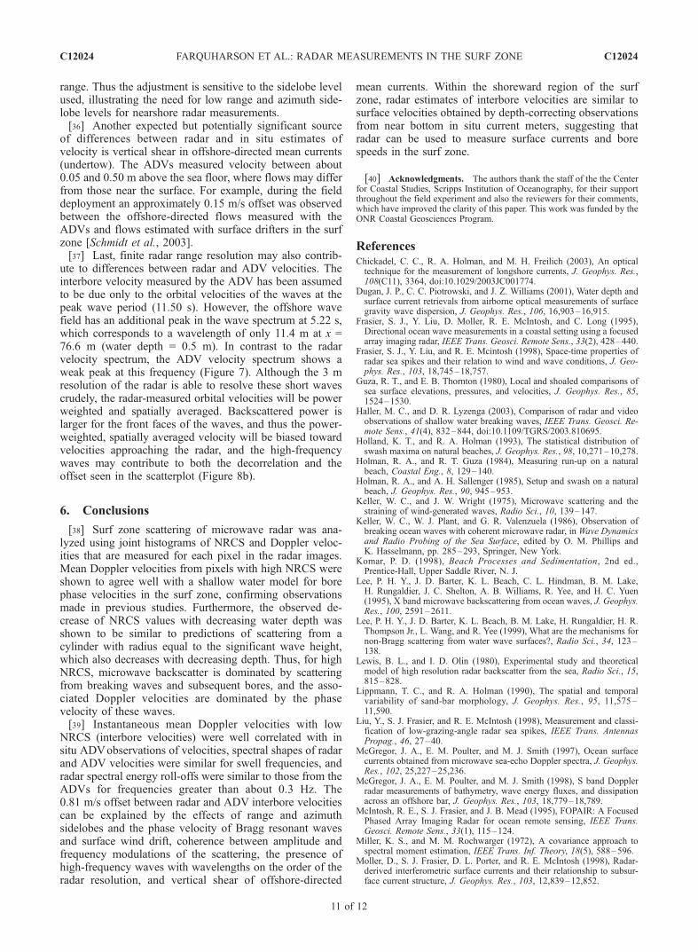
where the sidelobe power S1 is approximated as the peakNRCS for breaking waves (�14 dB in Figure 8a) minusthe estimated range gate leakage (�28 dB), the peakNRCS P2 is estimated as the peak value in a given NRCSrange, Cp is the mean phase velocity for the breaking waves(2.19 m/s), and the radar-measured Doppler velocity vd isbased on the velocity of each data point. Using nominalvalues for the Bragg resonant wave phase velocity vb =0.23 m/s and for the radial wind drift vw = 0.11 m/s (wheredrift is estimated as 3% of the 10 m wind speed of4.65 m/s), the adjusted Doppler velocity is computed fortwo NRCS ranges (�34 dB � s0 < �30 dB and �30 dB �s0 < �26 dB). After correcting for the sidelobe effects, theadjusted mean (vo + vc) radar radial velocity and the meanADV radial velocity for the lower (�34 dB � s0 < �30 dB,Figure 9a) NRCS conditional distributions are �0.06 and�0.23 m/s, respectively, and the adjusted mean radar radialvelocity and the mean ADV radial velocities for the upper(�30 dB � s0 < �26 dB, Figure 9b) NRCS conditional

Figure 6. Velocity versus time on 10 October 2000 between 1725 and 1730 UT. The solid curve is radarDoppler velocity at x = 76.6 m, y = 52.3 m, and the shaded curve is acoustic Doppler velocimeters (ADV)radial velocity at x = 76.0 m, y = 49.9 m. The approximately 3 m separation between the pixel used forthe radar Doppler velocity and the ADV frame is sufficient to prevent interference with the radarmeasurements. The data have been processed to a 2 Hz sample rate.

Figure 5. Predicted (asterisks) (equation (5)) and observed(diamonds) NRCS values versus cross-shore coordinate(and depth). Corresponding interbore NRCS values are�32 ± 2 dB.


8 of 12

C12024

distributions are 0.41 and �0.05 m/s, respectively. Thus,although the radar velocity distribution is broader than theADV distribution, the differences between the adjustedmean radar and mean ADV velocities have been reduced to0.17 m/s for the lower distribution and and 0.46 m/s for theupper distribution.[35] Correlation of amplitude and frequency modulations

of the Bragg scatterers [Keller and Wright, 1975] also maycontribute to the offset. At near-grazing angles, coherentpulse pair averages of 0.25 s are biased by up to 0.20 m/sfor upwind and up-wave conditions, compared with inco-

herent pulse pair averages [Moller et al., 1998]. Reprocess-ing the radar data using incoherent pulse pair averagingdoes not change the mean adjusted Doppler velocity for thelower NRCS range but reduces it from 0.41 to 0.34 m/s forthe upper NRCS range. Therefore some of the remainingdifference in radar and ADV mean velocity may be due tothe simplicity of the range and azimuth sidelobe modelused. Using a sidelobe level of �26 dB (2 dB less than thatused above) so that S1 = �40 dB reduces deviationsbetween mean radar and ADV velocities to 0.05 m/s forthe lower NRCS range and 0.25 m/s for the upper NRCS

Figure 7. (a) Energy density of Doppler (solid curve) and ADV radial (shaded dashed curve) velocity,(b) squared coherence, and (c) phase between Doppler and ADV velocity versus frequency for 20 mintime series. The 95% confidence limits on spectral estimates (0.04 Hz frequency resolution) are shown inFigure 7a, the 95% significance level for zero coherence is shown as a dashed horizontal line in Figure 7b,and the 95% confidence ranges on the phase estimates are shown as vertical bars through each symbol inFigure 7c. Phase estimates are shown only for squared coherence values that are larger than the 95%significance level.


9 of 12

C12024

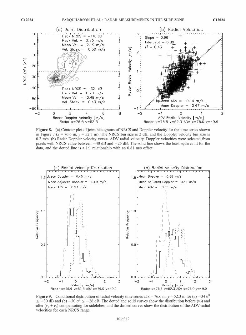
Figure 8. (a) Contour plot of joint histograms of NRCS and Doppler velocity for the time series shownin Figure 7 (x = 76.6 m, y = 52.3 m). The NRCS bin size is 2 dB, and the Doppler velocity bin size is0.2 m/s. (b) Radar Doppler velocity versus ADV radial velocity. Doppler velocities were selected frompixels with NRCS value between �40 dB and �25 dB. The solid line shows the least squares fit for thedata, and the dotted line is a 1:1 relationship with an 0.81 m/s offset.

Figure 9. Conditional distribution of radial velocity time series at x = 76.6 m, y = 52.3 m for (a) �34 s0

� �30 dB and (b) �30 s0 � �26 dB. The dotted and solid curves show the distribution before (vd) andafter (vo + vc) compensating for sidelobes, and the dashed curves show the distribution of the ADV radialvelocities for each NRCS range.


10 of 12

C12024

range. Thus the adjustment is sensitive to the sidelobe levelused, illustrating the need for low range and azimuth side-lobe levels for nearshore radar measurements.[36] Another expected but potentially significant source

of differences between radar and in situ estimates ofvelocity is vertical shear in offshore-directed mean currents(undertow). The ADVs measured velocity between about0.05 and 0.50 m above the sea floor, where flows may differfrom those near the surface. For example, during the fielddeployment an approximately 0.15 m/s offset was observedbetween the offshore-directed flows measured with theADVs and flows estimated with surface drifters in the surfzone [Schmidt et al., 2003].[37] Last, finite radar range resolution may also contrib-

ute to differences between radar and ADV velocities. Theinterbore velocity measured by the ADV has been assumedto be due only to the orbital velocities of the waves at thepeak wave period (11.50 s). However, the offshore wavefield has an additional peak in the wave spectrum at 5.22 s,which corresponds to a wavelength of only 11.4 m at x =76.6 m (water depth = 0.5 m). In contrast to the radarvelocity spectrum, the ADV velocity spectrum shows aweak peak at this frequency (Figure 7). Although the 3 mresolution of the radar is able to resolve these short wavescrudely, the radar-measured orbital velocities will be powerweighted and spatially averaged. Backscattered power islarger for the front faces of the waves, and thus the power-weighted, spatially averaged velocity will be biased towardvelocities approaching the radar, and the high-frequencywaves may contribute to both the decorrelation and theoffset seen in the scatterplot (Figure 8b).

6. Conclusions

[38] Surf zone scattering of microwave radar was ana-lyzed using joint histograms of NRCS and Doppler veloc-ities that are measured for each pixel in the radar images.Mean Doppler velocities from pixels with high NRCS wereshown to agree well with a shallow water model for borephase velocities in the surf zone, confirming observationsmade in previous studies. Furthermore, the observed de-crease of NRCS values with decreasing water depth wasshown to be similar to predictions of scattering from acylinder with radius equal to the significant wave height,which also decreases with decreasing depth. Thus, for highNRCS, microwave backscatter is dominated by scatteringfrom breaking waves and subsequent bores, and the asso-ciated Doppler velocities are dominated by the phasevelocity of these waves.[39] Instantaneous mean Doppler velocities with low

NRCS (interbore velocities) were well correlated with insitu ADVobservations of velocities, spectral shapes of radarand ADV velocities were similar for swell frequencies, andradar spectral energy roll-offs were similar to those from theADVs for frequencies greater than about 0.3 Hz. The0.81 m/s offset between radar and ADV interbore velocitiescan be explained by the effects of range and azimuthsidelobes and the phase velocity of Bragg resonant wavesand surface wind drift, coherence between amplitude andfrequency modulations of the scattering, the presence ofhigh-frequency waves with wavelengths on the order of theradar resolution, and vertical shear of offshore-directed

mean currents. Within the shoreward region of the surfzone, radar estimates of interbore velocities are similar tosurface velocities obtained by depth-correcting observationsfrom near bottom in situ current meters, suggesting thatradar can be used to measure surface currents and borespeeds in the surf zone.

[40] Acknowledgments. The authors thank the staff of the the Centerfor Coastal Studies, Scripps Institution of Oceanography, for their supportthroughout the field experiment and also the reviewers for their comments,which have improved the clarity of this paper. This work was funded by theONR Coastal Geosciences Program.

ReferencesChickadel, C. C., R. A. Holman, and M. H. Freilich (2003), An opticaltechnique for the measurement of longshore currents, J. Geophys. Res.,108(C11), 3364, doi:10.1029/2003JC001774.

Dugan, J. P., C. C. Piotrowski, and J. Z. Williams (2001), Water depth andsurface current retrievals from airborne optical measurements of surfacegravity wave dispersion, J. Geophys. Res., 106, 16,903–16,915.

Frasier, S. J., Y. Liu, D. Moller, R. E. McIntosh, and C. Long (1995),Directional ocean wave measurements in a coastal setting using a focusedarray imaging radar, IEEE Trans. Geosci. Remote Sens., 33(2), 428–440.

Frasier, S. J., Y. Liu, and R. E. Mcintosh (1998), Space-time properties ofradar sea spikes and their relation to wind and wave conditions, J. Geo-phys. Res., 103, 18,745–18,757.

Guza, R. T., and E. B. Thornton (1980), Local and shoaled comparisons ofsea surface elevations, pressures, and velocities, J. Geophys. Res., 85,1524–1530.

Haller, M. C., and D. R. Lyzenga (2003), Comparison of radar and videoobservations of shallow water breaking waves, IEEE Trans. Geosci. Re-mote Sens., 41(4), 832–844, doi:10.1109/TGRS/2003.810695.

Holland, K. T., and R. A. Holman (1993), The statistical distribution ofswash maxima on natural beaches, J. Geophys. Res., 98, 10,271–10,278.

Holman, R. A., and R. T. Guza (1984), Measuring run-up on a naturalbeach, Coastal Eng., 8, 129–140.

Holman, R. A., and A. H. Sallenger (1985), Setup and swash on a naturalbeach, J. Geophys. Res., 90, 945–953.

Keller, W. C., and J. W. Wright (1975), Microwave scattering and thestraining of wind-generated waves, Radio Sci., 10, 139–147.

Keller, W. C., W. J. Plant, and G. R. Valenzuela (1986), Observation ofbreaking ocean waves with coherent microwave radar, in Wave Dynamicsand Radio Probing of the Sea Surface, edited by O. M. Phillips andK. Hasselmann, pp. 285–293, Springer, New York.

Komar, P. D. (1998), Beach Processes and Sedimentation, 2nd ed.,Prentice-Hall, Upper Saddle River, N. J.

Lee, P. H. Y., J. D. Barter, K. L. Beach, C. L. Hindman, B. M. Lake,H. Rungaldier, J. C. Shelton, A. B. Williams, R. Yee, and H. C. Yuen(1995), X band microwave backscattering from ocean waves, J. Geophys.Res., 100, 2591–2611.

Lee, P. H. Y., J. D. Barter, K. L. Beach, B. M. Lake, H. Rungaldier, H. R.Thompson Jr., L. Wang, and R. Yee (1999), What are the mechanisms fornon-Bragg scattering from water wave surfaces?, Radio Sci., 34, 123–138.

Lewis, B. L., and I. D. Olin (1980), Experimental study and theoreticalmodel of high resolution radar backscatter from the sea, Radio Sci., 15,815–828.

Lippmann, T. C., and R. A. Holman (1990), The spatial and temporalvariability of sand-bar morphology, J. Geophys. Res., 95, 11,575–11,590.

Liu, Y., S. J. Frasier, and R. E. McIntosh (1998), Measurement and classi-fication of low-grazing-angle radar sea spikes, IEEE Trans. AntennasPropag., 46, 27–40.

McGregor, J. A., E. M. Poulter, and M. J. Smith (1997), Ocean surfacecurrents obtained from microwave sea-echo Doppler spectra, J. Geophys.Res., 102, 25,227–25,236.

McGregor, J. A., E. M. Poulter, and M. J. Smith (1998), S band Dopplerradar measurements of bathymetry, wave energy fluxes, and dissipationacross an offshore bar, J. Geophys. Res., 103, 18,779–18,789.

McIntosh, R. E., S. J. Frasier, and J. B. Mead (1995), FOPAIR: A FocusedPhased Array Imaging Radar for ocean remote sensing, IEEE Trans.Geosci. Remote Sens., 33(1), 115–124.

Miller, K. S., and M. M. Rochwarger (1972), A covariance approach tospectral moment estimation, IEEE Trans. Inf. Theory, 18(5), 588–596.

Moller, D., S. J. Frasier, D. L. Porter, and R. E. McIntosh (1998), Radar-derived interferometric surface currents and their relationship to subsur-face current structure, J. Geophys. Res., 103, 12,839–12,852.


11 of 12

C12024

Plant, W. J. (1990), Bragg scattering of electromagnetic waves from the air/sea interface, in Surface Waves and Fluxes, vol. 2, edited by G. L.Geernaert and W. J. Plant, chap. 11, pp. 41–108, Springer, New York.

Plant, W. J., E. A. Terray, R. A. J. Petitt, and W. C. Keller (1994), Thedependence of microwave backscatter from the sea on illuminated area:Correlation times and lengths, J. Geophys. Res., 99, 9705–9723.

Puleo, J. A., G. Farquharson, S. J. Frasier, and K. T. Holland (2003),Comparison of optical and radar measurements of surf and swash zonevelocity fields, J. Geophys. Res., 108(C3), 3100, doi:10.1029/2002JC001483.

Raubenheimer, B. (2002), Observations and predictions of fluid velocitiesin the surf and swash zones, J. Geophys. Res., 107(C11), 3190,doi:10.1029/2001JC001264.

Raubenheimer, B., R. T. Guza, and S. Elgar (1996), Wave transformationsacross the inner surf zone, J. Geophys. Res., 101, 25,589–25,597.

Schmidt, W. E., B. T. Woodward, K. S. Millikan, R. T. Guza,B. Raubenheimer, and S. Elgar (2003), A GPS-tracked surfzone drifter,J. Atmos. Oceanic Technol., 20, 1069–1075.

Sletten, M. A., J. C. West, X. Liu, and J. H. Duncan (2003), Radarinvestigations of breaking water waves at low grazing angles withsimultaneous high-speed optical imagery, Radio Sci., 38(6), 1110,doi:10.1029/2002RS002716.

Smith, J. A. (1993), Performance of a horizontally scanning Doppler sonarnear shore, J. Atmos. Oceanic Technol., 10, 752–763.

Smith, J. A., and J. L. Largier (1995), Observations of nearshore circula-tion: Rip currents, J. Geophys. Res., 100, 10,967–10,975.

Suhayda, J. N., and N. R. Pettigrew (1977), Observations of wave heightand wave celerity in the surf zone, J. Geophys. Res., 82, 1419–1424.

Thornton, E. B., and R. T. Guza (1982), Energy saturation and phase speedsmeasured on a natural beach, J. Geophys. Res., 87, 9499–9508.

Trizna, D. B. (2001), Errors in bathymetric retrievals using linear dispersionin 3-D FFT analysis of marine radar ocean wave imagery, IEEE Trans.Geosci. Remote Sens., 39(11), 2465–2469.

Valenzuela, G. R. (1968), Scattering of electromagnetic waves from a tiltedslightly rough surface, Radio Sci., 3, 1057–1066.

Wetzel, L. B. (1990), Electromagnetic scattering from the sea at low grazingangles, in Surface Wave and Fluxes, vol. 2, edited by G. L. Geernaert andW. J. Plant, chap. 12, pp. 109–171, Springer, New York.

Wright, J. W. (1968), A new model for sea clutter, IEEE Trans. AntennasPropag., 16, 217–223.

Young, I. R., W. Rosenthal, and F. Ziemer (1985), A three-dimensionalanalysis of marine radar images for the determination of oceanwave directionality and surface currents, J. Geophys. Res., 90,1049–1059.

��S. Elgar and B. Raubenheimer, Woods Hole Oceanographic Institution,

Woods Hole, MA 02543, USA. ([email protected]; [email protected])G. Farquharson, EOL, NCAR, 3450 Mitchell Lane, Building 1, Boulder,

CO 80301, USA. ([email protected])S. J. Frasier, Microwave Remote Sensing Laboratory, Department of

Electrical and Computer Engineering, University of Massachusetts,Amherst, MA 01003, USA. ([email protected])


12 of 12

C12024

microwave radar cross sections and doppler velocities ... · pdf filemicrowave radar cross...

Documents