mid-holocene vegetation in europe - cpd - · pdf filemid-holocene vegetation in europe ... l....
TRANSCRIPT
CPD5, 965–1011, 2009
Mid-Holocenevegetation in Europe
S. Brewer et al.
Title Page
Abstract Introduction
Conclusions References
Tables Figures
J I
J I
Back Close
Full Screen / Esc
Printer-friendly Version
Interactive Discussion
Clim. Past Discuss., 5, 965–1011, 2009www.clim-past-discuss.net/5/965/2009/© Author(s) 2009. This work is distributed underthe Creative Commons Attribution 3.0 License.
Climateof the Past
Discussions
Climate of the Past Discussions is the access reviewed discussion forum of Climate of the Past
Comparison of simulated and observedvegetation for the mid-Holocene in Europe
S. Brewer1, L. Francois1, R. Cheddadi2, J.-M. Laurent1, and E. Favre1
1Institut d’Astrophysique et de Geophysique, Universite de Liege, Bat. B5c, 17 Allee du SixAout, 4000 Liege, Belgium2Universite Montpellier II, Institut des Sciences de l’Evolution, case postale 61 CNRS UMR5554, 34095 Montpellier, France
Received: 21 October 2008 – Accepted: 21 October 2008 – Published: 13 March 2009
Correspondence to: S. Brewer ([email protected])
Published by Copernicus Publications on behalf of the European Geosciences Union.
965
CPD5, 965–1011, 2009
Mid-Holocenevegetation in Europe
S. Brewer et al.
Title Page
Abstract Introduction
Conclusions References
Tables Figures
J I
J I
Back Close
Full Screen / Esc
Printer-friendly Version
Interactive Discussion
Abstract
Past climates provide a testing bed for the predictive ability of general circulation mod-els. A number of studies have been performed for periods where the climate forcingsare relatively different from the present and there is a good coverage of data. For oneof these periods, the mid-Holocene (6 ka before present), models and data show a5
good match over northern Europe, but disagree over the south, where the data showcooler summers and winters and more humid conditions. Understanding the reasonsfor this disagreement is important given the expected vulnerability of the region underscenarios of future change. We present here a set of different past climate scenariosand sensitivity studies with a global vegetation model in order to try and understand10
this disagreement. The results show that the vegetation changes can be explained bya combination of both increased precipitation, and a reduction in the length of the grow-ing season, controlled by a reduction in winter temperatures. The matching simulatedcirculation patterns support the hypothesis of increased westerly flow over this region.
1 Introduction15
Simulating climates for past periods allow a test of the predictive ability of generalcirculation models (GCMs) under forcing conditions that are different to those of thepresent, including changes in orbital parameters, greenhouse gases and land surfaceconditions. Over the past few years, these tests have been the focus of the Paleocli-mate Model Intercomparison Project (PMIP, Braconnot et al., 2007). PMIP has been20
focused on two key periods, the mid-Holocene (MHL1) and the Last Glacial Maximum(LGM2). These two periods were chosen as there is a notable change in climate forc-ings compared to the present: insolation for MHL and ice sheet and atmospheric CO2content for the LGM. Further, both periods are relatively data-rich, due to a number of
16000 years before present221 000 years before present
966
CPD5, 965–1011, 2009
Mid-Holocenevegetation in Europe
S. Brewer et al.
Title Page
Abstract Introduction
Conclusions References
Tables Figures
J I
J I
Back Close
Full Screen / Esc
Printer-friendly Version
Interactive Discussion
synthesis projects (e.g. Biome6000; Prentice et al., 2000). The data include a range ofmacro- and micro-organisms that are climate proxies, i.e. have an indirect relation toone or more climate parameters. In terrestrial environments, fossil pollen assemblagesmake up the most common and widespread climate proxy, and are the data source formost continental comparisons.5
In order to compare the output of climate models and fossil pollen assemblages, thetwo data sources must be converted into compatible parameters. Comparisons aretherefore done in one of two ways, either by comparing climate reconstructed frompollen assemblages with that simulated by GCMs (e.g. Bonfils et al., 2004; Breweret al., 2007), or by finding the potential vegetation that corresponds to the simulated10
climate space and matching this to the vegetation reconstructed from pollen (Harrisonet al., 1998). For the European continent, the majority of these comparison studieshave been based on climate parameters (Masson et al., 1999; Bonfils et al., 2004;Brewer et al., 2007), due to the existence of a number of large-scale climate recon-structions (Cheddadi et al., 1997; Peyron et al., 1998; Davis et al., 2003). Recent15
developments including the use of fully coupled ocean-atmosphere GCMs (Braconnotet al., 2007), and better accounting for non-climatic conditions in climate reconstruc-tions have led to an improved agreement between models and data, notably for theLGM (Ramstein et al., 2007). However, there remains a mis-match for the MHL periodin southern Europe where the cooler and more humid summers reconstructed from the20
data are rarely simulated by the GCMs (Masson et al., 1999; Brewer et al., 2007). Un-der scenarios of future change, the Mediterranean is expected to be one of the areasthat is most affected. It is therefore important to understand the origins of this data-model disagreement, in order to assess their ability to predict climate in this regionunder different forcings.25
The mid-Holocene has been used in the PMIP project as most forcing parametersare similar to today, but there is a clear change in radiative forcing, with reduced winterinsolation (∼−6 W/m2) and increased summer insolation (∼+6 W/m2). Climatic recon-structions for Europe show that, instead of a direct response to these changes across
967
CPD5, 965–1011, 2009
Mid-Holocenevegetation in Europe
S. Brewer et al.
Title Page
Abstract Introduction
Conclusions References
Tables Figures
J I
J I
Back Close
Full Screen / Esc
Printer-friendly Version
Interactive Discussion
the continent, the climatic response varies on a north-south gradient (Cheddadi et al.,1997; Davis et al., 2003). In the south, winter temperatures are reduced, as a di-rect response, but in the north, winter warming occurs, due to a strengthening of thehigh pressure system over the Azores and an advection of warm air masses from theAtlantic Ocean (Masson et al., 1999). A similar pattern is observed in summer tem-5
peratures and growing season temperatures (represented as the sum of degree daysover 5◦C: GDD5), with an increase in the north and reduction in the south. Variations inwater budget also show a latitudinal trend, with drier conditions in the north of the conti-nent and wetter conditions to the south. This pattern in temperatures is not restricted tothe mid-Holocene, but forms part of a long-term opposition in climate changes between10
the north and south of Europe (Davis et al., 2003; Cheddadi and Bar-Hen, 2008).Simulations of mid-Holocene climate using atmospheric general circulation models
(GCMs) had mixed success in reproducing these observed changes (Masson et al.,1999). In general, the largest mis-match was in the south of Europe were no modelwas able to simulate the reduction in summer temperatures or GDD5 together with15
wetter conditions. This has led to criticisms of the reconstructions, suggesting that thevegetation change results from wetter conditions alone. Vegetation depends on theavailability of water, rather than the amount of precipitation, and this may be affectedby both rainfall and temperature. A sufficient increase in precipitation may thereforebe interpreted by a statistical climate reconstruction method as a reduction in temper-20
atures.At the global scale, the most significant change in vegetation cover for the MHL
period is the presence of a green Sahara, facilitated by the intensification of the AfricanMonsoon (Braconnot et al., 2000). In Europe, pollen based biome reconstructions arecharacterized by a general expansion of temperate forest to both the north and south25
with respect to the present (REF; Fig. 1). In the north, there is a general expansion oftemperate deciduous forest towards the north, replacing what is currently boreal forestand tundra. This follows a general poleward shift in forests seen across high latitudes(Prentice et al., 2000). In the Mediterranean region, there is an expansion of woodland
968
CPD5, 965–1011, 2009
Mid-Holocenevegetation in Europe
S. Brewer et al.
Title Page
Abstract Introduction
Conclusions References
Tables Figures
J I
J I
Back Close
Full Screen / Esc
Printer-friendly Version
Interactive Discussion
from the early to mid-Holocene (Huntley, 1988, 1990; Davis and Stevenson, 2007),with greater presence of temperate deciduous forest (Fig. 1). There also appears tobe a general reduction in the extent of grass and shrubland in this region, although itis unclear from the data whether this is simply due to the reduction in the number ofsites at this time. Overall, the distribution of vegetation suggests a reduced north-south5
difference in climate. The changes in Europe are relatively slight, when compared tothe LGM, and this presents a particular challenge for data-model comparison studies.
In the current study we avoid climatic interpretation of the pollen spectra, by com-paring the observed vegetation changes during the MHL period to vegetation sim-ulated using a global vegetation model CARAIB (Otto et al., 2002; Francois et al.,10
2006; Laurent et al., 2008) run using palaeo-GCM output. We investigate whether thelarge-scale changes in vegetation are reproduced in the models (e.g. treeline shifts),then we explore possible reasons for disagreements between data and models, usingfour different coupled ocean-atmosphere GCMs, which give a range of scenarios ofmid-Holocene climate change and therefore simulate different vegetation changes. By15
comparing the simulated climate between models with a good agreement, and thosewith a poor agreement, we attempt to identify the climate parameters that drove thepast changes in vegetation. Finally we test the sensitivity of the vegetation responseto different climatic parameters, including temperature, precipitation and atmosphericCO2 concentration.20
2 Methods
2.1 Data
Pollen data was obtained from the Biome 6000 project, version 4.23 (Prentice et al.,2000) as this currently provides the most complete global set of land cover conditions
3http://www.bridge.bris.ac.uk/resources/Databases/BIOMES data
969

CPD5, 965–1011, 2009
Mid-Holocenevegetation in Europe
S. Brewer et al.
Title Page
Abstract Introduction
Conclusions References
Tables Figures
J I
J I
Back Close
Full Screen / Esc
Printer-friendly Version
Interactive Discussion
for these two periods. We have used the European sub-region from the global data set(Prentice et al., 1996). The pollen assemblages for these sites have been classifiedinto one of 40 biomes, reclassed into a set of 13 mega-biomes, which are used here(Harrison and Prentice, 2003). These allow the changes in vegetation to be shown ina single synthetic map, and provide a first-order qualitative comparison with the model5
output. This dataset provided 3620 sites for the modern period (Fig. 1) and 462 sitesfor the mid-Holocene period (Fig. 1).
More recently, work by Laurent et al. (2004, 2008) has provided a finer grain classifi-cation, designed for both model and data. This is a set of 26 Bioclimatic Affinity Groups(BAGs, Laurent et al., 2004), defined using the modern climatic space of a set of 32010
European plant taxa. For this study, as we simply required a set of biogeographicaldistributions to provide clear and simple benchmarks for testing the GCM output, wehave retained the mega-biomes.
2.2 Vegetation modelling
The CARAIB vegetation model (Otto et al., 2002; Francois et al., 2006; Laurent et al.,15
2008) is a global vegetation model integrating a set of individual modules that providea detailed simulation of the carbon cycle and biogeography. Canopy photosynthesisand stomatal regulation are calculated using independent C3 (Farquhar et al., 1980)and C4 (Collatz et al., 1992) models, every two hours, with a daily update of plant andsoil carbon pools. The canopy contains 16 layers, including both tree and shrub/herb20
layers, which allows for light competition due to the absorption of radiation through thecanopy.
Water fluxes are calculated using a soil hydrological model (Francois et al., 2006).The soil water content is calculated on a daily basis. Input is provided the GCM sim-ulated precipitation, which is then divided into snow or rainfall according to the daily25
minimum and maximum temperatures. Snow accumulates in a surface snow reservoir,which can undergo melting and sublimation. Rain water can be intercepted by the fo-liage (depending on leaf area index, LAI) and either be re-evaporated (depending on
970
CPD5, 965–1011, 2009
Mid-Holocenevegetation in Europe
S. Brewer et al.
Title Page
Abstract Introduction
Conclusions References
Tables Figures
J I
J I
Back Close
Full Screen / Esc
Printer-friendly Version
Interactive Discussion
evaporative conditions) or produce throughfall. Snowmelt and throughfall are the twomain input fluxes for soil water. If their sum exceeds maximum infiltration (i.e., soilhydraulic conductivity at saturation), surface runoff is produced. A single reservoir ofsoil water is used, which corresponds to the root zone, and drainage from this is basedon the hydraulic conductivity. Actual evapotranspiration (AET) from the soil/vegetation5
layer is calculated as a fraction of Penman’s potential evapotranspiration (Penman,1948), depending on soil wetness. Soil water availability can affect stomatal conduc-tance, leaf area index and plant mortality. Transpiration fluxes calculated from stomatalconductance and photosynthetic rates in the carbon cycle module cannot exceed theAET flux calculated by the soil hydrological module. This criterion allows to define a10
maximum value of the species LAI, on a monthly (herbs/shrubs) or seasonal/annual(trees) basis. Volumetric soil water amounts at wilting point, field capacity and satura-tion, as well as soil hydraulic conductivity, are functions of soil texture (Saxton et al.,1986).
The biogeography module is based on climatic thresholds defined for each group that15
is simulated. The most important of these control the establishment of plant groups orspecies and are based on a) the growing season, defined by a minimum number ofgrowing degree days above 5◦C (GDD5); b) a period of cold temperatures in wintercontrolling germination; and c) the existence of a dry period during the year. Plantmortality may also be affected by cold and/or drought events, defined by the coldest20
day and by soil water availability, as described above. An offline scheme is used totranslate the modelled cover and LAI for all plant groups in a given grid cell into abiome class, permitting the model biome distribution to be mapped.
The inputs to CARAIB are a set of climate parameters, including temperature, pre-cipitation, percentage sunshine, wind speed, relative humidity and diurnal temperature25
range. These values are required as a set of 12 monthly values for each grid cell.Daily values are produced with a stochastic weather generator (Hubert et al., 1998). Inaddition, the atmospheric concentration of CO2, orbital parameters and soil texture arerequired.
971
CPD5, 965–1011, 2009
Mid-Holocenevegetation in Europe
S. Brewer et al.
Title Page
Abstract Introduction
Conclusions References
Tables Figures
J I
J I
Back Close
Full Screen / Esc
Printer-friendly Version
Interactive Discussion
Modern vegetation cover was simulated using conditions as close to pre-industrial aspossible. The climatology was calculated from the CRU TS2.0 gridded dataset at a res-olution of 0.5×0.5◦. Values were estimated as the average of monthly values between1901 and 1950 (Mitchell and Jones, 2005), to minimise the effect of recent warming.Atmospheric CO2 concentration was set to 279 ppm (Indermuhle et al., 1999). The5
modern distribution of vegetation is shown in Fig. 2.For the mid-Holocene period, the CARAIB model was driven by output taken from
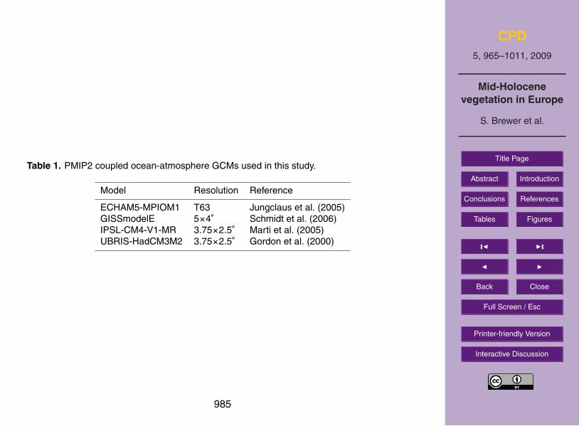
four coupled ocean-atmosphere GCMs from the most recent PMIP comparison exper-iment, chosen to represent a range of mid-Holocene change scenarios. Details of the4 GCMs used (ECHAM5-MPIOM1, GISSmodelE, IPSL-CM4-V1-MR, HadCM3M2) are10
given in Table 1.In order to obtain input for the vegetation model, monthly anomalies were calculated
for each parameter required as the simulated mid-Holocene climate less the controlclimate. The anomalies were then interpolated to a 0.5◦ grid and added to the modernclimatology, as described in Francois et al. (1998, 1999). Atmospheric CO2 concentra-15
tion was set to 264 ppm (Indermuhle et al., 1999).Sensitivity tests were performed to attempt to isolate the effects of different cli-
mate parameters. Four tests were performed (Table 2): a) mid-Holocene climate withmodern (pre-industrial) atmospheric CO2 levels (VClim); b) pre-industrial climate withmid-Holocene atmospheric CO2 levels (VCO2); c) pre-industrial temperature and mid-20
Holocene precipitation values (VPRC); d) mid-Holocene temperature and pre-industrialprecipitation values (VTEM). Other climate inputs were held at the mid-Holocene for ex-periments VClim, VPRC and VTEM, and at pre-industrial values for VCO2. Only theresults obtained from the GISSmodelE sensitivity tests are shown here.
3 Results25
We have simulated both the biomes distributions and the net primary productivity. Allclimate models forced CARAIB to simulate a switch from a general dominance of tem-
972
CPD5, 965–1011, 2009
Mid-Holocenevegetation in Europe
S. Brewer et al.
Title Page
Abstract Introduction
Conclusions References
Tables Figures
J I
J I
Back Close
Full Screen / Esc
Printer-friendly Version
Interactive Discussion
perate deciduous forest in the centre of the continent to cool temperate forest (Fig. 3)and their expansion northward into Scandinavia. This expansion is most notable in Fin-land and North-west Russia. The distribution of tundra and boreal montane biomes isreduced in all simulations, most clearly usingthe IPSL-CM4-V1-MR climatology (Figs. 3and 4). To help interpret this vegetation dynamics we have investigated the changes5
in soil water availability and the length and intensity of the growing season for the fourGCMs.
– The ECHAM5-MPIOM1 simulation (Fig. 3a) shows a very similar distribution ofbiomes to the pre-industrial simulation, with some small increases in the distribu-tion of grassland and semi-desertic biomes in Northern Africa.10
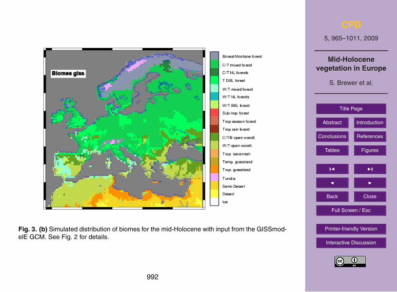
– The GISSmodelE simulation (Fig. 3b) shows different changes in the west andeast of the Mediterranean basin, with a southward expansion of warm/temperateopen forest, most notably in Northern Africa where it replaces grassland and semi-desert, and an increase of warm/temperate mixed forest in the Iberian peninsula,indicating a closing of the forest. In the south-east, warm/temperate open forest15
expand northward in the Balkan peninsula.
– The IPSL-CM4-V1-MR simulation (Fig. 3c) shows a more widespread opening ofthe forest in the southeast, reaching up into the Pannonian basin, but little changefrom the present in the south-west.
– The expansion of the warm/temperate open forest using simulations from the20
HadCM3M2 (Fig. 3d) and the GISSmodelE (Fig. 3b) is similar. In both caseswe observe an expansion southward in the west and northward in the east.
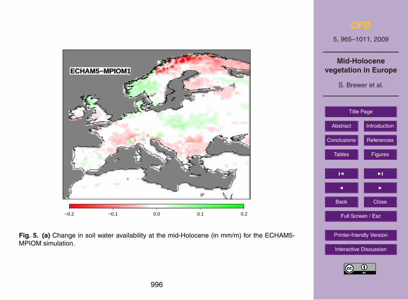
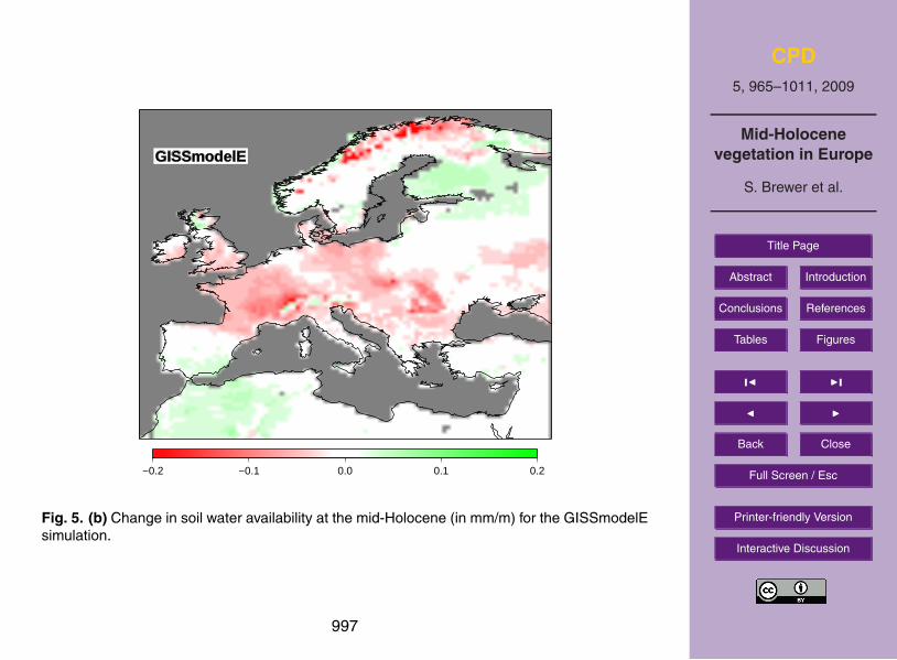
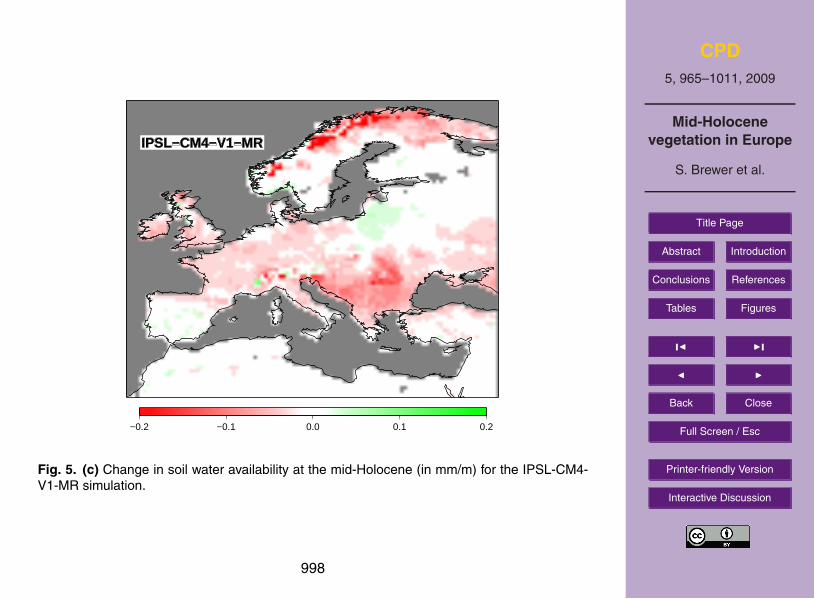
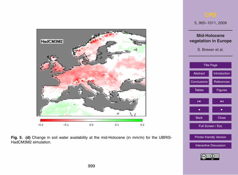
The soil water availability changes (Fig. 5) are similar from all four GCM input, with anoverall decrease in northern Scandinavia, due to the warmer and dryer conditions andan increase in the Iberian peninsula. The output from ECHAM5-MPIOM also shows25
a slight increase in eastern Europe, north of the Carpathian mountain chain, and the
973

CPD5, 965–1011, 2009
Mid-Holocenevegetation in Europe
S. Brewer et al.
Title Page
Abstract Introduction
Conclusions References
Tables Figures
J I
J I
Back Close
Full Screen / Esc
Printer-friendly Version
Interactive Discussion
HadCM3M2 simulations shows some drying in North-West Europe (France and theUK).
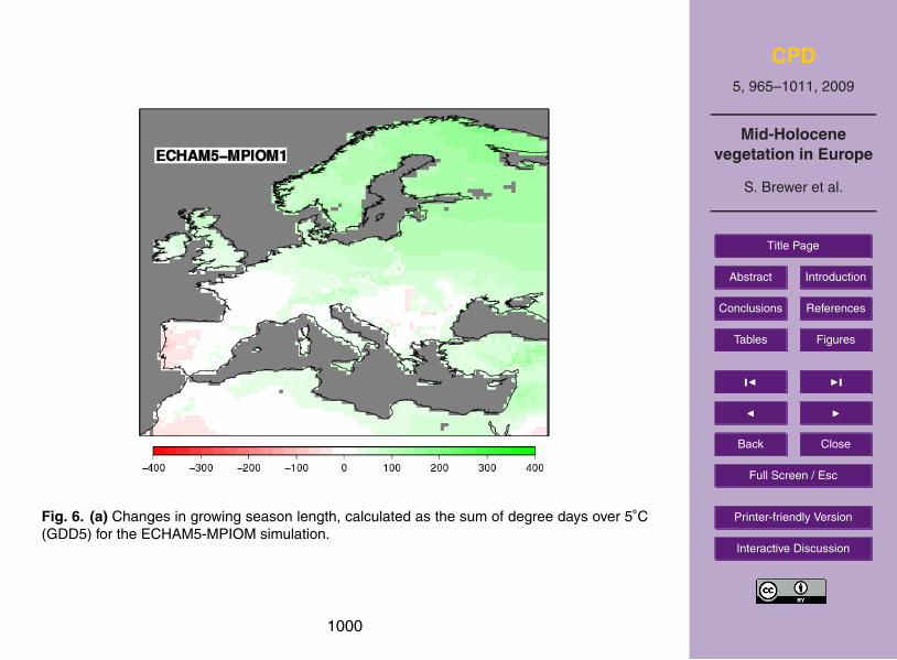
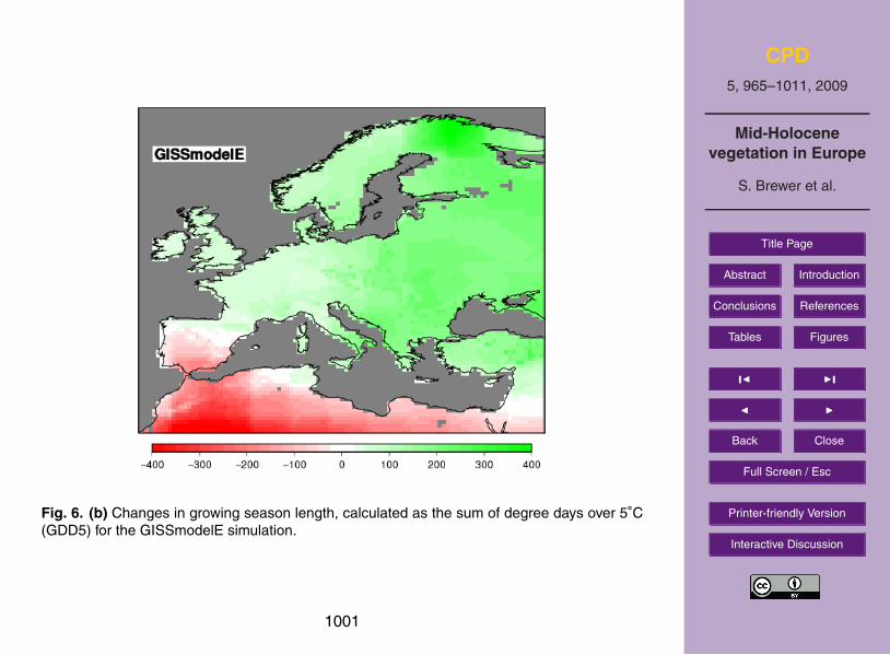
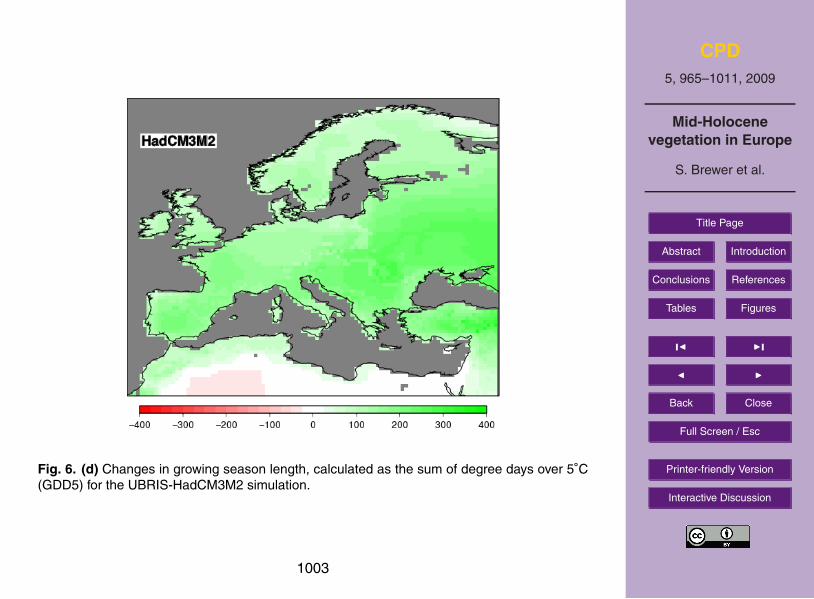
The GDD5 (Fig. 6) shows a general increase across Europe for all simulations. Thistends to form a gradient from high values in the north-east to lower values and somereduction in GDD5 values in the south-west. The exception to this is GISSmodelE,5
which shows a marked lowering across the south of the study area. The simulatedbiomes distributions for the mid-Holocene (Fig. 3) show a greater variation betweenmodel output in the south of the continent.
The simulated net primary productivity (NPP) shows a general decline (Fig. 7) duringthe mid-Holocene when compared to the pre-industrial period (Table 3). There is also10
some regional variation between the north-west, north-east, south-west and south-eastof Europe (Fig. 5). While all regions show a range of positive and negative values, theresults show the largest reductions in the northern regions, with in general (over 75% ofpixels) a decline. The reduction is less marked in the south, shown by a median closeto zero. The simulations are again more varied in the south-west, with HadCM3M215
simulations showing a balance of increases and decreases, and an overall trend toincreased NPP in the GISSmodelE simulation.
4 Discussion
In this discussion of the results, we first compare the simulated vegetation distributionsagainst observations, in order to identify the GCM output that provides the best agree-20
ment. The robustness of the simulations is also tested by comparison with two previoussimulations of European MHL vegetation. We then try and isolate the climate factorsdriving this vegetation shift by examining a) changes in the simulated GCM monthly cli-matologies; and b) the effect of changing different parameters on the MHL vegetationdistribution, which also allows us to account for the role played by the slight change25
in atmospheric CO2 concentration. Finally, we use the information obtained to test ahypothesis of mid-Holocene circulation change over the study area.
974

CPD5, 965–1011, 2009
Mid-Holocenevegetation in Europe
S. Brewer et al.
Title Page
Abstract Introduction
Conclusions References
Tables Figures
J I
J I
Back Close
Full Screen / Esc
Printer-friendly Version
Interactive Discussion
The simulated changes in the vegetation cover of Europe obtained in this study showlittle difference to the modern day potential cover, and the results obtained from theoutput of the different GCMs are very similar. This is unsurprising given the relativelysmall climatic changes between the mid-Holocene and the pre-industrial climatologyused here. The most notable and consistent change is in the composition of the forest5
cover of the centre of Europe, with a change to a slightly cooler forest type. Pollenspectra from this time show a transition from an early Holocene forest dominated byPinus, Betula, Corylus and Quercus to one composed of Fagus, Picea, Carpinus andQuercus (Huntley, 1990). The simulated biome distribution therefore offers a view ofthe potential vegetation cover prior to the acceleration of human impact in the sec-10
ond half of the Holocene (Roberts, 1998; Marchant et al., 2009). The relatively smallchange also suggests that, within the climatic changes between the mid-Holocene andthe pre-industrial, the vegetation distribution of Europe is fairly stable in its structure, ifnot in its composition.
In the north of Europe, the observed poleward spread of temperate forests is ob-15
served in all the simulations, although there is less expansion in Sweden and Norwaythan in the data. Pollen sequences suggest that this expansion covered between 50and 100 km (Kaplan et al., 2003), and this agrees with the expansion in Finland andnorthwest Russia. In contrast, while an overall reduction of tundra is observed in allmodels (Fig. 4), there is no clear geographical representation of this (Fig. 3). This is20
at least in part due to the different methods of classifying tundra in the data and themodels. Tundra biome is simulated in CARAIB when GDD5 values and/or LAI valuesdrop below a certain threshold, whereas the pollen tundra biomes are based on repre-sentivity of a set of plant functional types (Prentice et al., 1996). Boundaries betweensimulated tundra and other biomes tend to be more sharply defined, causing a differ-25
ence in geographical distribution. This is particularly noticeable for the modern pollenbiome distribution, where tundra is recreated in a few pollen samples in southern Eu-rope. This is due to a high presence of species found in anthropogenic heathlands,which have a similar composition of pollen taxa, while differing in the plant specific
975

CPD5, 965–1011, 2009
Mid-Holocenevegetation in Europe
S. Brewer et al.
Title Page
Abstract Introduction
Conclusions References
Tables Figures
J I
J I
Back Close
Full Screen / Esc
Printer-friendly Version
Interactive Discussion
composition (Prentice et al., 1996).The observed changes in the south of Europe are more complex, and varied between
the four GCMs. Simulated biome distributions from two of these (ECHAM-MPIOM1 andIPSL-CM4-V1-MR) show no distinct change from the modern distribution. In contrast,the remaining two GCMs do show a development of an open forest type, particularly in5
the southwest, at the expense of the grassland cover, which matches the descriptionof an expansion of forest in the Mediterranean (Huntley, 1990; Davis and Stevenson,2007). The observed southward expansion of deciduous temperate forest (Fig. 1) isnot seen in the simulations. This supports previous studies indicating that althoughthe direction of the simulated mid-Holocene climate change may be correct, the ampli-10
tude is not (Brewer et al., 2007). However, it should be noted that there are few datapoints in the centre of the Iberian peninsula (Fig. 1). A recent study of sites situatedin the Ebro desert suggest that the increased precipitation during this period was notlarge enough to support large populations of temperate deciduous trees (Davis andStevenson, 2007), indicating a landscape closer to that obtained from GISSmodelE15
and HadCM3M2.The disagreements between observed and simulated MHL vegetation described
above are similar to that found in previous studies. Prentice et al. (1998) simulatedbiome distribution for the mid-Holocene, using the BIOME model with output fromNCAR CCM1 GCM, coupled to a mixed layer ocean model. As with the present re-20
sults, they found an insufficient northward extension of deciduous forests and little of nosouthward extension. They also note a simulated expansion of steppe-like vegetationto the north of the Black Sea, as found here in the IPSL and HadCM3M2 simulations.Kaplan et al. (2003) compared simulated and observed vegetation north of 55◦ N us-ing the BIOME4 model and two coupled ocean-atmosphere GCMs. Their results also25
showed that while deciduous forests expanded in Fennoscandia, this is less than thatobserved in the data, due to insufficient winter warming.
Based on the comparison of the different vegetation simulations, the GISSmodelErun simulates changes that are the closest to the observations, notably in the south-
976

CPD5, 965–1011, 2009
Mid-Holocenevegetation in Europe
S. Brewer et al.
Title Page
Abstract Introduction
Conclusions References
Tables Figures
J I
J I
Back Close
Full Screen / Esc
Printer-friendly Version
Interactive Discussion
west. In order to identify the climatic changes that drove these changes, we comparethe anomaly climatologies for each GCM (Fig. 9). The temperature anomalies show aclear shift to a more seasonal climate, and that the influence of the insolation changes(Berger, 1978) dominates this climatic parameter.
The climatologies show little evidence for winter warming in the north, with most5
temperature changes close to zero. The exceptions are the ECHAM5-MPIOM1 model(Fig. 8) in the northwest and the IPSL-CM4-V1-MR model in the NE (Fig. 8). Warmerwinters are necessary for the observed expansion in deciduous and mixed forests inFennoscandia (Prentice et al., 1998) and this explains the limited response in the sim-ulations. As these are regional averages, there may have been some greater but lo-10
calised warming, and the pattern of treeline shifts suggests that there was a land-seagradient, with greater warming toward the continental interior. This is consistent withreconstructed warmer winter temperatures in the east of Europe (Davis et al., 2003).Precipitation changes in the north show no obvious pattern with a mixture of positiveand negative anomalies. One exception to this is the ECHAM5-MPIOM1 simulation,15
which shows a general increase in precipitation throughout the year.In the south, changes in precipitation appear to play the most important role. An
increase in summer precipitation is seen in both models (GISSmodelE, HadCM3M2)that show the same type of vegetation change as in the data, i.e. towards greater for-est cover in the south-west (Figs. 8b and d). The GISSmodelE also shows a general20
cooling throughout the year, with a much smaller summer increase than the other mod-els, suggesting that temperature change may also have helped drive the vegetationchanges. In the south-east, an increase in precipitation is simulated by the ECHAM5-MPIOM1 model throughout the majority of the year, and this is the only model to notshow an expansion of steppe vegetation in this region.25
In terms of parameters that control the distribution of plants more directly, thesechanges translate into an increase in soil water availability (Fig. 5) and a decrease inGDD5 (Fig. 6). However, while all models show an increase in soil water in the Iberianpeninsula, that covers a greater or lesser spatial area, an expansion of forest types
977
CPD5, 965–1011, 2009
Mid-Holocenevegetation in Europe
S. Brewer et al.
Title Page
Abstract Introduction
Conclusions References
Tables Figures
J I
J I
Back Close
Full Screen / Esc
Printer-friendly Version
Interactive Discussion
is not seen in all simulations. This supports the role of temperature changes in themid-Holocene vegetation, in particular a marked lowering of GDD5. This change is ofinterest, as it shows that this variable is controlled by winter temperature changes inthe south of Europe, and a reduction may occur, even when the summer temperatureincreases.5
The results show a general decline in NPP for the mid-Holocene across Europe (Ta-ble 3), with regional variations (Fig. 7). This fits with the slight decline in mid-Holoceneglobal NPP described by Beerling and Woodward (2001), using two GCMs, althoughthe variations given by these authors for the European latitudes are very close to mod-ern values. However, the results obtained by Peng et al. (1998), using a statistical mod-10
elling approach based on pollen data, show an increase in NPP for this period. Thissecond study does not explicitly model the photosynthetic process, and does not takeinto account the small change in atmospheric CO2 concentration at the mid-Holocene.
From the sensitivity experiments (Fig. 9), it is possible to attribute the decline inNPP in the east of Europe to both changes in climate (VClim) and CO2 (VCO2) con-15
centration. Equally, while winter temperature played an important role in changing thecomposition of the forests in the north-east (Prentice et al., 2000), and water availabilityin the south-east (Prentice et al., 2000), experiments with modern temperature (VPRC)or modern precipitation (VTEM) indicate that productivity in these regions was affectedby changes in both these variables.20
In the north-west, changing CO2 concentration alone results in a decrease of NPPequal to approximately 50% of the combined climate and CO2 effect. In contrast, whenCO2 is kept at modern levels and climate changed, this reduction is much smaller.This may be due to a strong gradient of climate anomalies in this region. Holding pre-cipitation or temperature to modern values causes a similar reduction, although the25
mid-Holocene temperatures cause a larger change when compared to modern val-ues. Productivity increases in the south-west during the mid-Holocene. The sensitivityexperiments suggest that this increase comes from the climate change, offset by a re-duction due to lower CO2 concentration. Changing precipitation appears to account for
978

CPD5, 965–1011, 2009
Mid-Holocenevegetation in Europe
S. Brewer et al.
Title Page
Abstract Introduction
Conclusions References
Tables Figures
J I
J I
Back Close
Full Screen / Esc
Printer-friendly Version
Interactive Discussion
all of the climatically induced NPP changes, whereas temperature has little effect.In general, the change due to CO2 concentration variation is relatively high, matching
the effect of climate change in east of Europe. However, these changes are small, andfurther work will be necessary to test the sensitivity of CARAIB to CO2.
Bonfils et al. (2004) proposed a scenario of circulation changes to explain the ob-5
served mid-Holocene winter climate in Europe. We examine here whether the GCMproviding the best fit to the data in this study (GISSmodelE) supports this. The sce-nario is based on the existence of an anomalous low pressure system located overnorth-west Europe causing an increased westerly flow over the south-west and bring-ing moisture into the Mediterranean basin. Any heating from the advection of these air10
masses was offset by the reduction in insolation (Bonfils, 2001; Bonfils et al., 2004).Having lost moisture, the air masses then flowed north were the smaller insolationanomalies were no longer sufficient to prevent warming.
Changes in surface wind from the GISSmodelE simulation, which provided the bestfit to the data, support this scenario (Fig. 10), with a clear counter-clockwise and in-15
creased westerly flow over the Mediterranean. This is, however, slightly displaced tothe north and west compared to Bonfils et al. (2004), and this may have limited theadvection of moisture towards the interior, resulting in the reduced moisture availabil-ity in south eastern Europe. A similar pattern can be seen in both the HadCM3M2and ECHAM5-MPIOM GCMs, but in both cases, the area of low pressure is positioned20
further to the north-west. This limits the westerly flow in the HadCM3M2 model andresults in a more southerly flow in the ECHAM5-MPIOM. This pattern appears to beabsent in the IPSL-CM4-V1-MR wind patterns (Fig. 10).
5 Conclusions
– Simulated vegetation distributions based on coupled ocean-atmosphere GCMs25
show a poleward shift in Fennoscandia, with a corresponding loss of tundra andboreal montane forest, that are consistent with the observed changes.
979

CPD5, 965–1011, 2009
Mid-Holocenevegetation in Europe
S. Brewer et al.
Title Page
Abstract Introduction
Conclusions References
Tables Figures
J I
J I
Back Close
Full Screen / Esc
Printer-friendly Version
Interactive Discussion
– In central Europe there is a change in forest composition in central Europeanforests toward a dominance of cool temperate forest types.
– The observed southward spread of temperate forests is not observed in anymodel, but two simulations show an increase in forest cover, with loss of desert,semi-desert and temperate grasslands.5
– Changes in the south are driven by increased moisture availability, but lower win-ter temperatures also played a role. In the Mediterranean region, a decrease inthe relatively higher winter temperatures leads to a decrease in GDD5, which maybe reconstructed as lower summer temperatures.
– The observed pattern of changes is consistent with increased westerly flow from10
Atlantic, bringing increased precipitation over the Mediterranean basin.
Acknowledgements. Financial support for the study was provided by FRFC conventionno. 2.4555.06. The work forms part of project DECVEG from the European Science Foun-dation (ESF) under the EUROCORES Programme EuroCLIMATE, through contract No. ERAS-CT-2003-980409 of the European Commission, DG Research, FP6. We thank the PMIP215
Database (http://pmip2.lsce.ipsl.fr/) for providing GCM data.
Publication of this paper was granted by EDD (Environnement, Developpement Durable)and INSU (Institut des Sciences de l’Univers) at CNRS.
References20
Beerling, D. and Woodward, F.: Vegetation and the Terrestrial Carbon Cycle: Modelling theFirst 400 Million Years, Cambridge University Press, 2001. 978
980

CPD5, 965–1011, 2009
Mid-Holocenevegetation in Europe
S. Brewer et al.
Title Page
Abstract Introduction
Conclusions References
Tables Figures
J I
J I
Back Close
Full Screen / Esc
Printer-friendly Version
Interactive Discussion
Berger, A.: Long-term variations of daily insolation and Quaternary climatic changes, J. Atmos.Sci., 35, 2362–2367, 1978. 977
Bonfils, C.: Le moyen-Holocene: role de la surface continentale sur la sensibilite climatiquesimulee, Ph.D. thesis, Universite Paris VI, Paris, 322 pp., 2001. 979
Bonfils, C., de Noblet-Ducoudre, N., Guiot, J., and Bartlein, P. J.: Some mechanisms of mid-5
Holocene climate change in Europe, inferred from comparing PMIP models to data, Clim.Dynam., 23, 79–98, 2004. 967, 979
Braconnot, P., Joussaume, S., de Noblet, N., and Ramstein, G.: Mid-Holocene and last glacialmaximum African monsoon changes as simulated within the Paleoclimate Modeling Inter-comparison project, Global Planet. Change, 26, 51–66, 2000. 96810
Braconnot, P., Otto-Bliesner, B., Harrison, S., Joussaume, S., Peterchmitt, J.-Y., Abe-Ouchi, A.,Crucifix, M., Driesschaert, E., Fichefet, Th., Hewitt, C. D., Kageyama, M., Kitoh, A., Laıne, A.,Loutre, M.-F., Marti, O., Merkel, U., Ramstein, G., Valdes, P., Weber, S. L., Yu, Y., and Zhao,Y.: Results of PMIP2 coupled simulations of the Mid-Holocene and Last Glacial Maximum –Part 1: experiments and large-scale features, Clim. Past, 3, 261–277, 2007,15
http://www.clim-past.net/3/261/2007/. 966, 967Brewer, S., Guiot, J., and Torre, F.: Mid-Holocene climate change in Europe: a data-model
comparison, Clim. Past, 3, 499–512, 2007,http://www.clim-past.net/3/499/2007/. 967, 976
Cheddadi, R. and Bar-Hen, A.: Spatial gradient of temperature and potential vegetation feed-20
back across Europe during the late Quaternary, Clim. Dynam., 32(2–3), 371–379, 2008.968
Cheddadi, R., Yu, G., Guiot, J., Harrison, S. P., and Prentice, I. C.: The climate of Europe 6000years ago, Clim. Dynam., 13, 1–9, 1997. 967, 968
Collatz, G., Ribas-Carbo, M., and Berry, J.: Coupled photosynthesis-stomatal conductance25
model for leaves of C4 plants, Aust. J. Plant Physiol., 19, 519–538, 1992. 970Davis, B. A. S. and Stevenson, A. C.: The 8.2 ka event and early mid-Holocene forests, fires
and flooding in the Central Ebro Desert, NE Spain, Quaternary Sci. Rev., 26, 1695–1712,2007. 969, 976
Davis, B. A. S., Brewer, S., Stevenson, A. C., Guiot, J., and Data contributors: The temperature30
of Europe during the Holocene reconstructed from pollen data, Quaternary Sci. Rev., 22,1701–1716, 2003. 967, 968, 977
Farquhar, G., von Caellerer, S., and Berry, J.: A biogeochemical model of photosynthetic CO2
981

CPD5, 965–1011, 2009
Mid-Holocenevegetation in Europe
S. Brewer et al.
Title Page
Abstract Introduction
Conclusions References
Tables Figures
J I
J I
Back Close
Full Screen / Esc
Printer-friendly Version
Interactive Discussion
assimilation in leaves of C3 species, Planta, 149, 78–90, 1980. 970Francois, L., Delire, C., Warnant, P., and Munhoven, G.: Modelling the glacial-interglacial
changes in the continental biosphere, Global Planet. Change, 16–17, 37–52, 1998. 972Francois, L., Godderis, Y., Warnant, P., Ramstein, G., de Noblet, N., and Lorenz, S.: Carbon
stocks and isotopic budgets of the terrestrial biosphere at mid-Holocene and last glacial5
maximum times, Chem. Geol., 159, 163–189, 1999. 972Francois, L., Ghislain, M., Otto, D., and Micheels, A.: Late Miocene vegetation reconstruction
with the CARAIB model, Palaeogeography, Palaeoclimatology, Palaeoecology, 238, 302–320, 2006. 969, 970
Harrison, S. P. and Prentice, I. C.: Climate and CO2 controls on global vegetation distribution10
at the last glacial maximum: analysis based on palaeovegetation data, biome modelling andpalaeoclimate simulations, Global Change Biol., 9, 983–1004. 970
Harrison, S., Jolly, D., Laarif, F., Abe-Ouchi, A., Dong, B., Herterich, K., Hewitt, C. D., Jous-saume, S., Kutzbach, J., Mitchell, J., De Noblet, N., and Valdes, P.: Intercomparison ofsimulated global vegetation distributions in response to 6 kyr BP orbital forcing, J. Climate,15
11, 2721–2742, 1998. 967Hubert, B., Francois, L., Warnant, P., and Strivay, D.: Stochastic generation of meteorological
variables and effects on global models of water and carbon cycles in vegetation and soils, J.Hydrol., 212–213, 318–334, 1998. 971
Huntley, B.: Europe, in: Vegetation History, edited by: Huntley, B. and Webb III, T., 341–383,20
Kluwer Academic Publishers, New York, 1988. 969Huntley, B.: European post-glacial forests: compositional chnages in response to climatic
change, J. Veg. Sci., 1, 507–518, 1990. 969, 975, 976Indermuhle, A., Stocker, T. F., Joos, F., Fischer, H., Smith, H. J., Wahlen, M., Deck, B., Mas-
troianni, D., Tschumi, J., Blunier, T., Meyer, R., and Stauffer, B.: Holocene carbon-cycle25
dynamics based on CO2 trapped in ice at Taylor Dome, Antarctica, Nature, 398, 121–126,doi:10.1038/18158, 1999. 972
Kaplan, J. O., Bigelow, N. H., Prentice, I. C., Harrison, S. P., Bartlein, P. J., Christensen, T. R.,Cramer, W., Matveyeva, N. V., McGuire, A. D., Murray, D. F., Razzhivin, V. Y., Smith, B.,Walker, D. A., Anderson, P. M., Andreev, A. A., Brubaker, L. B., Edwards, M. E., and Lozhkin,30
A. V.: Climate change and arctic ecosystems II: Modeling, paleodata-model comparisons,and future projections, J. Geophys. Res., 108, 8171, doi:10.1029/2002JD002559, 2003. 975,976
982

CPD5, 965–1011, 2009
Mid-Holocenevegetation in Europe
S. Brewer et al.
Title Page
Abstract Introduction
Conclusions References
Tables Figures
J I
J I
Back Close
Full Screen / Esc
Printer-friendly Version
Interactive Discussion
Laurent, J.-M., Bar-Hen, A., Francois, L., Ghislain, M., and Cheddadi, R.: Refining vegetationsimulation models: From plant functional types to bioclimatic affinity groups of plants, J. Veg.Sci., 15, 739–746, 2004. 970
Laurent, J.-M., Francois, L., Bar-Hen, A., Bel, L., and Cheddadi, R.: European BioclimaticAffinity Groups: data-model comparisons, Global Planet. Change, 61, 28–40, doi:10.1016/j.5
gloplacha.2007.08.017, 2008. 969, 970Marchant, R., Brewer, S., Webb III, T., and Turvey, S.: Holocene deforestation: a history of
human-environmental interactions, climate change and extinction, in: Holocene Extinctions,edited by: Turvey, S., Oxford University Press, in press, 2009. 975
Masson, V., Cheddadi, R., Braconnot, P., Joussaume, S., Texier, D., and PMIP Participants:10
Mid-Holocene climate in Europe: what can we infer from PMIP model-data comparisons?,Clim. Dynam., 15, 163–182, 1999. 967, 968
Mitchell, T. and Jones, P.: An improved method of constructing a database of monthly climateobservations and associated high-resolution grids, Int. J. Climatol., 25, 693–712, 2005. 972
Otto, D., Rasse, D., Kaplan, J., Warnant, P., and Francois, L.: Biospheric carbon stocks recon-15
structed at the Last Glacial Maximum: comparison between general circulation models usingprescribed and computed sea surface temperatures, Global Planet. Change, 33, 117–138,2002. 969, 970
Penman, H.: Natural evaporation from open water, bare soil and grass, Proc. Roy. Soc. Ser. A,193, 120–145, 1948. 97120
Peyron, O., Guiot, J., Cheddadi, R., Tarasov, P., Reille, M., De Beaulieu, J. L., Bottema, S.,and Andrieu, V.: Climatic Reconstruction in Europe for 18,000 Yr B.p. From Pollen Data,Quaternary Res., 49, 183–196, 1998. 967
Prentice, I., Jolly, D., and Biome 6000 Participants: Mid-Holocene and glacial-maximum veg-etation geography of the northern continents and Africa, J. Biogeogr., 27, 507–519, doi:25
10.1046/j.1365-2699.2000.00425.x, 2000. 967, 968, 969, 978Prentice, I. C., Guiot, J., Huntley, B., Jolly, D., and Cheddadi, R.: Reconstructing biomes from
palaeoecological data: a general method and its application to European pollen data at 0and 6 ka, Clim. Dynam., 12, 184–194, 1996. 970, 975, 976
Prentice, I. C., Harrison, S., Jolly, D., and Guiot, J.: The climate and biomes of Europe at 600030
yr BP: comparison of model simulations and pollen-based reconstructions, Quaternary Sci.Rev., 17, 659–668, 1998. 976, 977
Ramstein, G., Kageyama, M., Guiot, J., Wu, H., Hely, C., Krinner, G., and Brewer, S.: How cold
983
CPD5, 965–1011, 2009
Mid-Holocenevegetation in Europe
S. Brewer et al.
Title Page
Abstract Introduction
Conclusions References
Tables Figures
J I
J I
Back Close
Full Screen / Esc
Printer-friendly Version
Interactive Discussion
was Europe at the Last Glacial Maximum? A synthesis of the progress achieved since thefirst PMIP model-data comparison, Clim. Past, 3, 331–339, 2007,http://www.clim-past.net/3/331/2007/. 967
Roberts, N.: The Holocene: an environmental history, Blackwell, 1998. 975Saxton, K., Rawls, W., Romberger, J., and Papendick, R.: Estimating generalized soil-water5
characteristics from texture, Soil Sci. Soc. Am. J., 50, 1031–1036, 1986. 971
984
CPD5, 965–1011, 2009
Mid-Holocenevegetation in Europe
S. Brewer et al.
Title Page
Abstract Introduction
Conclusions References
Tables Figures
J I
J I
Back Close
Full Screen / Esc
Printer-friendly Version
Interactive Discussion
Table 1. PMIP2 coupled ocean-atmosphere GCMs used in this study.
Model Resolution Reference
ECHAM5-MPIOM1 T63 Jungclaus et al. (2005)GISSmodelE 5×4◦ Schmidt et al. (2006)IPSL-CM4-V1-MR 3.75×2.5◦ Marti et al. (2005)UBRIS-HadCM3M2 3.75×2.5◦ Gordon et al. (2000)
985

CPD5, 965–1011, 2009
Mid-Holocenevegetation in Europe
S. Brewer et al.
Title Page
Abstract Introduction
Conclusions References
Tables Figures
J I
J I
Back Close
Full Screen / Esc
Printer-friendly Version
Interactive Discussion
Table 2. List of experiments performed during this study and associated variables. Temp:monthly temperature; Prec: monthly precipitation; CO2: Atmospheric concentration; Other: allother climatic parameters. “0 ka” indicates that the pre-industrial values of that variable wereused; “6 ka” indicates that mid-Holocene values were used.
Experiment Temp. Prec. CO2 conc. Other
PREIND 0 ka 0 ka 0 ka 0 kaMHL 6 ka 6 ka 6 ka 6 kaVClim 6 ka 6 ka 0 ka 6 kaVCO2 0 ka 0 ka 6 ka 0 kaVPRC 0 ka 6 ka 6 ka 6 kaVTEM 6 ka 0 ka 6 ka 6 ka
986
CPD5, 965–1011, 2009
Mid-Holocenevegetation in Europe
S. Brewer et al.
Title Page
Abstract Introduction
Conclusions References
Tables Figures
J I
J I
Back Close
Full Screen / Esc
Printer-friendly Version
Interactive Discussion
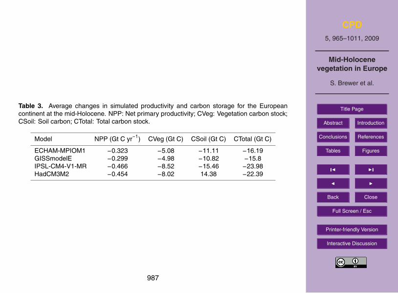
Table 3. Average changes in simulated productivity and carbon storage for the Europeancontinent at the mid-Holocene. NPP: Net primary productivity; CVeg: Vegetation carbon stock;CSoil: Soil carbon; CTotal: Total carbon stock.
Model NPP (Gt C yr−1) CVeg (Gt C) CSoil (Gt C) CTotal (Gt C)
ECHAM-MPIOM1 −0.323 −5.08 −11.11 −16.19GISSmodelE −0.299 −4.98 −10.82 −15.8IPSL-CM4-V1-MR −0.466 −8.52 −15.46 −23.98HadCM3M2 −0.454 −8.02 14.38 −22.39
987

CPD5, 965–1011, 2009
Mid-Holocenevegetation in Europe
S. Brewer et al.
Title Page
Abstract Introduction
Conclusions References
Tables Figures
J I
J I
Back Close
Full Screen / Esc
Printer-friendly Version
Interactive Discussion
Biomes 0ka BP
TrFo WTFo SaSh GrSh Dese TeFo BoFo Tund DrTn
Fig. 1. (a) Distribution of biomes in Europe at 0 ka. TrFo = Tropical forest; WTFo = Warmtemperate forest; SaSh = Savannah/shrubland; GrSh Grassland/Shrubland; Dese = Desert;TeFo = Temperate forest; BoFo = Boreal forest; Tund = Tundra; DrTn = Dry tundra.
988

CPD5, 965–1011, 2009
Mid-Holocenevegetation in Europe
S. Brewer et al.
Title Page
Abstract Introduction
Conclusions References
Tables Figures
J I
J I
Back Close
Full Screen / Esc
Printer-friendly Version
Interactive Discussion
Biomes 6ka BP
TrFo WTFo SaSh GrSh Dese TeFo BoFo Tund DrTn
Fig. 1. (b) Distribution of biomes in Europe at the mid-Holocene. See Fig. 1a for caption.
989
CPD5, 965–1011, 2009
Mid-Holocenevegetation in Europe
S. Brewer et al.
Title Page
Abstract Introduction
Conclusions References
Tables Figures
J I
J I
Back Close
Full Screen / Esc
Printer-friendly Version
Interactive Discussion
4 S. Brewer et al.: Mid-Holocene vegetation in Europe
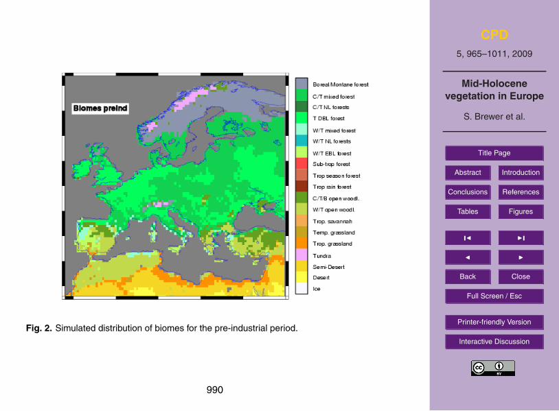
Fig. 2. Simulated distribution of biomes for the pre-industrial pe-riod.
ing. Atmospheric CO2 concentration was set to 279ppm (In-dermuhle et al., 1999). The modern distribution of vegetation215
is shown in figure 2.For the mid-Holocene period, the CARAIB model was
driven by output taken from four coupled ocean-atmosphereGCMs from the most recent PMIP comparison experiment,chosen to represent a range of mid-Holocene change sce-220
narios. Details of the 4 GCMs used (ECHAM5-MPIOM1,GISSmodelE, IPSL-CM4-V1-MR, HadCM3M2) are givenin table 1.
In order to obtain input for the vegetation model, monthlyanomalies were calculated for each parameter required as225
the simulated mid-Holocene climate less the control climate.The anomalies were then interpolated to a 0.5 grid and addedto the modern climatology, as described in Francois et al.(1998, 1999). Atmospheric CO2 concentration was set to264ppm (Indermuhle et al., 1999).230
Sensitivity tests were performed to attempt to isolate theeffects of different climate parameters. Four tests were per-formed (table 2): a) mid-Holocene climate with modern (pre-industrial) atmospheric CO2 levels (VClim); b) pre-industrialclimate with mid-Holocene atmospheric CO2 levels (VCO2);235
c) pre-industrial temperature and mid-Holocene precipita-tion values (VPRC); d) mid-Holocene temperature and pre-industrial precipitation values (VTEM). Other climate in-puts were held at the mid-Holocene for experiments VClim,VPRC and VTEM, and at pre-industrial values for VCO2.240
Only the results obtained from the GISSmodelE simulationare shown here.
3 Results
We have simulated both the biomes distributions and the netprimary productivity. All climate models forced CARAIB to245
Fig. 3a. Simulated distribution of biomes for the mid-Holocenewith input from the ECHAM5-MPIOM1 GCM. See figure 2 fordetails.
Fig. 3b. Simulated distribution of biomes for the mid-Holocenewith input from the GISSmodelE GCM. See figure 2 for details.
simulate a switch from a general dominance of temperate de-ciduous forest in the centre of the continent to cool temperateforest (figure 3) and their expansion northward into Scandi-navia. This expansion is most notable in Finland and North-west Russia. The distribution of tundra and boreal montane250
biomes is reduced in all simulations, most clearly usingtheIPSL-CM4-V1-MR climatology (figure 3c and 4). To helpinterpret this vegetation dynamics we have investigated thechanges in soil water availability and the length and intensityof the growing season for the four GCMs.255
– The ECHAM5-MPIOM1 simulation (figure 3a) shows avery similar distribution of biomes to the pre-industrialsimulation, with some small increases in the distribu-
Fig. 2. Simulated distribution of biomes for the pre-industrial period.
990

CPD5, 965–1011, 2009
Mid-Holocenevegetation in Europe
S. Brewer et al.
Title Page
Abstract Introduction
Conclusions References
Tables Figures
J I
J I
Back Close
Full Screen / Esc
Printer-friendly Version
Interactive Discussion
4 S. Brewer et al.: Mid-Holocene vegetation in Europe
Fig. 2. Simulated distribution of biomes for the pre-industrial pe-riod.
ing. Atmospheric CO2 concentration was set to 279ppm (In-dermuhle et al., 1999). The modern distribution of vegetation215
is shown in figure 2.For the mid-Holocene period, the CARAIB model was
driven by output taken from four coupled ocean-atmosphereGCMs from the most recent PMIP comparison experiment,chosen to represent a range of mid-Holocene change sce-220
narios. Details of the 4 GCMs used (ECHAM5-MPIOM1,GISSmodelE, IPSL-CM4-V1-MR, HadCM3M2) are givenin table 1.
In order to obtain input for the vegetation model, monthlyanomalies were calculated for each parameter required as225
the simulated mid-Holocene climate less the control climate.The anomalies were then interpolated to a 0.5 grid and addedto the modern climatology, as described in Francois et al.(1998, 1999). Atmospheric CO2 concentration was set to264ppm (Indermuhle et al., 1999).230
Sensitivity tests were performed to attempt to isolate theeffects of different climate parameters. Four tests were per-formed (table 2): a) mid-Holocene climate with modern (pre-industrial) atmospheric CO2 levels (VClim); b) pre-industrialclimate with mid-Holocene atmospheric CO2 levels (VCO2);235
c) pre-industrial temperature and mid-Holocene precipita-tion values (VPRC); d) mid-Holocene temperature and pre-industrial precipitation values (VTEM). Other climate in-puts were held at the mid-Holocene for experiments VClim,VPRC and VTEM, and at pre-industrial values for VCO2.240
Only the results obtained from the GISSmodelE simulationare shown here.
3 Results
We have simulated both the biomes distributions and the netprimary productivity. All climate models forced CARAIB to245
Fig. 3a. Simulated distribution of biomes for the mid-Holocenewith input from the ECHAM5-MPIOM1 GCM. See figure 2 fordetails.
Fig. 3b. Simulated distribution of biomes for the mid-Holocenewith input from the GISSmodelE GCM. See figure 2 for details.
simulate a switch from a general dominance of temperate de-ciduous forest in the centre of the continent to cool temperateforest (figure 3) and their expansion northward into Scandi-navia. This expansion is most notable in Finland and North-west Russia. The distribution of tundra and boreal montane250
biomes is reduced in all simulations, most clearly usingtheIPSL-CM4-V1-MR climatology (figure 3c and 4). To helpinterpret this vegetation dynamics we have investigated thechanges in soil water availability and the length and intensityof the growing season for the four GCMs.255
– The ECHAM5-MPIOM1 simulation (figure 3a) shows avery similar distribution of biomes to the pre-industrialsimulation, with some small increases in the distribu-
Fig. 3. (a) Simulated distribution of biomes for the mid-Holocene with input from the ECHAM5-MPIOM1 GCM. See Fig. 2 for details.
991
CPD5, 965–1011, 2009
Mid-Holocenevegetation in Europe
S. Brewer et al.
Title Page
Abstract Introduction
Conclusions References
Tables Figures
J I
J I
Back Close
Full Screen / Esc
Printer-friendly Version
Interactive Discussion
4 S. Brewer et al.: Mid-Holocene vegetation in Europe
Fig. 2. Simulated distribution of biomes for the pre-industrial pe-riod.
ing. Atmospheric CO2 concentration was set to 279ppm (In-dermuhle et al., 1999). The modern distribution of vegetation215
is shown in figure 2.For the mid-Holocene period, the CARAIB model was
driven by output taken from four coupled ocean-atmosphereGCMs from the most recent PMIP comparison experiment,chosen to represent a range of mid-Holocene change sce-220
narios. Details of the 4 GCMs used (ECHAM5-MPIOM1,GISSmodelE, IPSL-CM4-V1-MR, HadCM3M2) are givenin table 1.
In order to obtain input for the vegetation model, monthlyanomalies were calculated for each parameter required as225
the simulated mid-Holocene climate less the control climate.The anomalies were then interpolated to a 0.5 grid and addedto the modern climatology, as described in Francois et al.(1998, 1999). Atmospheric CO2 concentration was set to264ppm (Indermuhle et al., 1999).230
Sensitivity tests were performed to attempt to isolate theeffects of different climate parameters. Four tests were per-formed (table 2): a) mid-Holocene climate with modern (pre-industrial) atmospheric CO2 levels (VClim); b) pre-industrialclimate with mid-Holocene atmospheric CO2 levels (VCO2);235
c) pre-industrial temperature and mid-Holocene precipita-tion values (VPRC); d) mid-Holocene temperature and pre-industrial precipitation values (VTEM). Other climate in-puts were held at the mid-Holocene for experiments VClim,VPRC and VTEM, and at pre-industrial values for VCO2.240
Only the results obtained from the GISSmodelE simulationare shown here.
3 Results
We have simulated both the biomes distributions and the netprimary productivity. All climate models forced CARAIB to245
Fig. 3a. Simulated distribution of biomes for the mid-Holocenewith input from the ECHAM5-MPIOM1 GCM. See figure 2 fordetails.
Fig. 3b. Simulated distribution of biomes for the mid-Holocenewith input from the GISSmodelE GCM. See figure 2 for details.
simulate a switch from a general dominance of temperate de-ciduous forest in the centre of the continent to cool temperateforest (figure 3) and their expansion northward into Scandi-navia. This expansion is most notable in Finland and North-west Russia. The distribution of tundra and boreal montane250
biomes is reduced in all simulations, most clearly usingtheIPSL-CM4-V1-MR climatology (figure 3c and 4). To helpinterpret this vegetation dynamics we have investigated thechanges in soil water availability and the length and intensityof the growing season for the four GCMs.255
– The ECHAM5-MPIOM1 simulation (figure 3a) shows avery similar distribution of biomes to the pre-industrialsimulation, with some small increases in the distribu-
Fig. 3. (b) Simulated distribution of biomes for the mid-Holocene with input from the GISSmod-elE GCM. See Fig. 2 for details.
992

CPD5, 965–1011, 2009
Mid-Holocenevegetation in Europe
S. Brewer et al.
Title Page
Abstract Introduction
Conclusions References
Tables Figures
J I
J I
Back Close
Full Screen / Esc
Printer-friendly Version
Interactive Discussion
S. Brewer et al.: Mid-Holocene vegetation in Europe 5
Fig. 3c. Simulated distribution of biomes for the mid-Holocenewith input from the IPSL-CM4-V1-MR GCM. See figure 2 for de-tails.
Fig. 3d. Simulated distribution of biomes for the mid-Holocenewith input from the UBris-HadCM3M2 GCM. See figure 2 for de-tails.
tion of grassland and semi-desertic biomes in NorthernAfrica.260
– The GISSmodelE simulation (figure 3b) shows differ-ent changes in the west and east of the Mediterraneanbasin, with a southward expansion of warm/temperateopen forest, most notably in Northern Africa where itreplaces grassland and semi-desert, and an increase of265
warm/temperate mixed forest in the Iberian peninsula,indicating a closing of the forest. In the south-east,warm/temperate open forest expand northward in theBalkan peninsula.
– The IPSL-CM4-V1-MR simulation (figure 3c) shows a270
DESE SEDE TUND TRGR TEGR WTOF CTBO WTEB WTMX TEDE CTMX BOMO
Echam5GISSIPSLUBris
050
100
150
Fig. 4. Mid-Holocene cover of simulated biomes as as percentagesof modern cover. DESE = Desert; SEDE = Semi-desert; TUND =Tundra; TRGR = Tropical grassland; TEGR = Temperate grassland;WTOF = Warm temperate open forest; CTBO = Cool temperate bo-real forest; WTEB = Warm temperate evergreen broadleaved forest;WTMX = Warm temperate mixed forest; TEDE = Temperate de-ciduous forest; CTMX = Cool temperate mixed; BOMO = Borealmontane forest.
more widespread opening of the forest in the southeast,reaching up into the Pannonian basin, but little changefrom the present in the south-west.
– The expansion of the warm/temperate open forest us-ing simulations from the HadCM3M2 (figure 3d) and275
the GISSmodelE (figure 3b) is similar. In both cases weobserve an expansion southward in the west and north-ward in the east.
The soil water availability (figure 5) is similar from allfour GCM input, with an overall decrease in northern Scan-280
dinavia, due to the warmer and dryer conditions and an in-crease in the Iberian peninsula. The output from ECHAM5-MPIOM also shows a slight increase in eastern Europe, northof the Carpathian mountain chain, and the HadCM3M2 sim-ulations shows some drying in North-West Europe (France285
and the UK).The GDD5 (figure 6) shows a general increase across Eu-
rope for all simulations. This tends to form a gradient fromhigh values in the north-east to lower values and some reduc-tion in GDD5 values in the south-west. The exception to this290
is GISSmodelE, which shows a marked lowering across thesouth of the study area. The simulated biomes distributionsfor the mid-Holocene (figure 3) show a greater variation be-tween model output in the south of the continent.
The simulated net primary productivity (NPP) shows a295
general decline (figures 7) during the mid-Holocene whencompared to the pre-industrial period (table 3). There is alsosome regional variation between the north-west, north-east,south-west and south-east of Europe (figure 5). While allregions show a range of positive and negative values, the re-300
Fig. 3. (c) Simulated distribution of biomes for the mid-Holocene with input from the IPSL-CM4-V1-MR GCM. See Fig. 2 for details.
993

CPD5, 965–1011, 2009
Mid-Holocenevegetation in Europe
S. Brewer et al.
Title Page
Abstract Introduction
Conclusions References
Tables Figures
J I
J I
Back Close
Full Screen / Esc
Printer-friendly Version
Interactive Discussion
S. Brewer et al.: Mid-Holocene vegetation in Europe 5
Fig. 3c. Simulated distribution of biomes for the mid-Holocenewith input from the IPSL-CM4-V1-MR GCM. See figure 2 for de-tails.
Fig. 3d. Simulated distribution of biomes for the mid-Holocenewith input from the UBris-HadCM3M2 GCM. See figure 2 for de-tails.
tion of grassland and semi-desertic biomes in NorthernAfrica.260
– The GISSmodelE simulation (figure 3b) shows differ-ent changes in the west and east of the Mediterraneanbasin, with a southward expansion of warm/temperateopen forest, most notably in Northern Africa where itreplaces grassland and semi-desert, and an increase of265
warm/temperate mixed forest in the Iberian peninsula,indicating a closing of the forest. In the south-east,warm/temperate open forest expand northward in theBalkan peninsula.
– The IPSL-CM4-V1-MR simulation (figure 3c) shows a270
DESE SEDE TUND TRGR TEGR WTOF CTBO WTEB WTMX TEDE CTMX BOMO
Echam5GISSIPSLUBris
050
100
150
Fig. 4. Mid-Holocene cover of simulated biomes as as percentagesof modern cover. DESE = Desert; SEDE = Semi-desert; TUND =Tundra; TRGR = Tropical grassland; TEGR = Temperate grassland;WTOF = Warm temperate open forest; CTBO = Cool temperate bo-real forest; WTEB = Warm temperate evergreen broadleaved forest;WTMX = Warm temperate mixed forest; TEDE = Temperate de-ciduous forest; CTMX = Cool temperate mixed; BOMO = Borealmontane forest.
more widespread opening of the forest in the southeast,reaching up into the Pannonian basin, but little changefrom the present in the south-west.
– The expansion of the warm/temperate open forest us-ing simulations from the HadCM3M2 (figure 3d) and275
the GISSmodelE (figure 3b) is similar. In both cases weobserve an expansion southward in the west and north-ward in the east.
The soil water availability (figure 5) is similar from allfour GCM input, with an overall decrease in northern Scan-280
dinavia, due to the warmer and dryer conditions and an in-crease in the Iberian peninsula. The output from ECHAM5-MPIOM also shows a slight increase in eastern Europe, northof the Carpathian mountain chain, and the HadCM3M2 sim-ulations shows some drying in North-West Europe (France285
and the UK).The GDD5 (figure 6) shows a general increase across Eu-
rope for all simulations. This tends to form a gradient fromhigh values in the north-east to lower values and some reduc-tion in GDD5 values in the south-west. The exception to this290
is GISSmodelE, which shows a marked lowering across thesouth of the study area. The simulated biomes distributionsfor the mid-Holocene (figure 3) show a greater variation be-tween model output in the south of the continent.
The simulated net primary productivity (NPP) shows a295
general decline (figures 7) during the mid-Holocene whencompared to the pre-industrial period (table 3). There is alsosome regional variation between the north-west, north-east,south-west and south-east of Europe (figure 5). While allregions show a range of positive and negative values, the re-300
Fig. 3. (d) Simulated distribution of biomes for the mid-Holocene with input from the UBris-HadCM3M2 GCM. See Fig. 2 for details.
994

CPD5, 965–1011, 2009
Mid-Holocenevegetation in Europe
S. Brewer et al.
Title Page
Abstract Introduction
Conclusions References
Tables Figures
J I
J I
Back Close
Full Screen / Esc
Printer-friendly Version
Interactive Discussion
DESE SEDE TUND TRGR TEGR WTOF CTBO WTEB WTMX TEDE CTMX BOMO
Echam5GISSIPSLUBris
050
100
150
Fig. 4. Mid-Holocene cover of simulated biomes as as percentages of modern cover. DESE =Desert; SEDE = Semi-desert; TUND = Tundra; TRGR = Tropical grassland; TEGR = Temper-ate grassland; WTOF = Warm temperate open forest; CTBO = Cool temperate boreal forest;WTEB = Warm temperate evergreen broadleaved forest; WTMX = Warm temperate mixed for-est; TEDE = Temperate deciduous forest; CTMX = Cool temperate mixed; BOMO = Borealmontane forest.
995
CPD5, 965–1011, 2009
Mid-Holocenevegetation in Europe
S. Brewer et al.
Title Page
Abstract Introduction
Conclusions References
Tables Figures
J I
J I
Back Close
Full Screen / Esc
Printer-friendly Version
Interactive Discussion
ECHAM5−MPIOM1
−0.2 −0.1 0.0 0.1 0.2
Fig. 5. (a) Change in soil water availability at the mid-Holocene (in mm/m) for the ECHAM5-MPIOM simulation.
996
CPD5, 965–1011, 2009
Mid-Holocenevegetation in Europe
S. Brewer et al.
Title Page
Abstract Introduction
Conclusions References
Tables Figures
J I
J I
Back Close
Full Screen / Esc
Printer-friendly Version
Interactive Discussion
GISSmodelE
−0.2 −0.1 0.0 0.1 0.2
Fig. 5. (b) Change in soil water availability at the mid-Holocene (in mm/m) for the GISSmodelEsimulation.
997
CPD5, 965–1011, 2009
Mid-Holocenevegetation in Europe
S. Brewer et al.
Title Page
Abstract Introduction
Conclusions References
Tables Figures
J I
J I
Back Close
Full Screen / Esc
Printer-friendly Version
Interactive Discussion
IPSL−CM4−V1−MR
−0.2 −0.1 0.0 0.1 0.2
Fig. 5. (c) Change in soil water availability at the mid-Holocene (in mm/m) for the IPSL-CM4-V1-MR simulation.
998
CPD5, 965–1011, 2009
Mid-Holocenevegetation in Europe
S. Brewer et al.
Title Page
Abstract Introduction
Conclusions References
Tables Figures
J I
J I
Back Close
Full Screen / Esc
Printer-friendly Version
Interactive Discussion
HadCM3M2
−0.2 −0.1 0.0 0.1 0.2
Fig. 5. (d) Change in soil water availability at the mid-Holocene (in mm/m) for the UBRIS-HadCM3M2 simulation.
999
CPD5, 965–1011, 2009
Mid-Holocenevegetation in Europe
S. Brewer et al.
Title Page
Abstract Introduction
Conclusions References
Tables Figures
J I
J I
Back Close
Full Screen / Esc
Printer-friendly Version
Interactive Discussion
S. Brewer et al.: Mid-Holocene vegetation in Europe 7
Fig. 6a. Changes in growing season length, calculated as the sumof degree days over 5◦C (GDD5) for the ECHAM5-MPIOM simu-lation
Fig. 6b. Changes in growing season length, calculated as the sumof degree days over 5◦C (GDD5) for the GISSmodelE simulation
simulated GCM monthly climatologies; and b) the effect ofchanging different parameters on the MHL vegetation distri-bution, which also allows us to account for the role playedby the slight change in atmospheric CO2 concentration. Fi-nally, we use the information obtained to test a hypothesis of320
mid-Holocene circulation change over the study area.The simulated changes in the vegetation cover of Europe
obtained in this study show little difference to the modern
Fig. 6c. Changes in growing season length, calculated as the sumof degree days over 5◦C (GDD5) for the IPSL-CM4-V1-MR simu-lation
Fig. 6d. Changes in growing season length, calculated as the sumof degree days over 5◦C (GDD5) for the UBRIS-HadCM3M2 sim-ulation
day potential cover, and the results obtained from the outputof the different GCMs are very similar. This is unsurpris-325
ing given the relatively small climatic changes between themid-Holocene and the pre-industrial climatology used here.The most notable change is in the composition of the forestcover of the centre of Europe, with a change to a slightlycooler forest type. Pollen spectra from this time show a330
Fig. 6. (a) Changes in growing season length, calculated as the sum of degree days over 5◦C(GDD5) for the ECHAM5-MPIOM simulation.
1000
CPD5, 965–1011, 2009
Mid-Holocenevegetation in Europe
S. Brewer et al.
Title Page
Abstract Introduction
Conclusions References
Tables Figures
J I
J I
Back Close
Full Screen / Esc
Printer-friendly Version
Interactive Discussion
S. Brewer et al.: Mid-Holocene vegetation in Europe 7
Fig. 6a. Changes in growing season length, calculated as the sumof degree days over 5◦C (GDD5) for the ECHAM5-MPIOM simu-lation
Fig. 6b. Changes in growing season length, calculated as the sumof degree days over 5◦C (GDD5) for the GISSmodelE simulation
simulated GCM monthly climatologies; and b) the effect ofchanging different parameters on the MHL vegetation distri-bution, which also allows us to account for the role playedby the slight change in atmospheric CO2 concentration. Fi-nally, we use the information obtained to test a hypothesis of320
mid-Holocene circulation change over the study area.The simulated changes in the vegetation cover of Europe
obtained in this study show little difference to the modern
Fig. 6c. Changes in growing season length, calculated as the sumof degree days over 5◦C (GDD5) for the IPSL-CM4-V1-MR simu-lation
Fig. 6d. Changes in growing season length, calculated as the sumof degree days over 5◦C (GDD5) for the UBRIS-HadCM3M2 sim-ulation
day potential cover, and the results obtained from the outputof the different GCMs are very similar. This is unsurpris-325
ing given the relatively small climatic changes between themid-Holocene and the pre-industrial climatology used here.The most notable change is in the composition of the forestcover of the centre of Europe, with a change to a slightlycooler forest type. Pollen spectra from this time show a330
Fig. 6. (b) Changes in growing season length, calculated as the sum of degree days over 5◦C(GDD5) for the GISSmodelE simulation.
1001

CPD5, 965–1011, 2009
Mid-Holocenevegetation in Europe
S. Brewer et al.
Title Page
Abstract Introduction
Conclusions References
Tables Figures
J I
J I
Back Close
Full Screen / Esc
Printer-friendly Version
Interactive Discussion
S. Brewer et al.: Mid-Holocene vegetation in Europe 7
Fig. 6a. Changes in growing season length, calculated as the sumof degree days over 5◦C (GDD5) for the ECHAM5-MPIOM simu-lation
Fig. 6b. Changes in growing season length, calculated as the sumof degree days over 5◦C (GDD5) for the GISSmodelE simulation
simulated GCM monthly climatologies; and b) the effect ofchanging different parameters on the MHL vegetation distri-bution, which also allows us to account for the role playedby the slight change in atmospheric CO2 concentration. Fi-nally, we use the information obtained to test a hypothesis of320
mid-Holocene circulation change over the study area.The simulated changes in the vegetation cover of Europe
obtained in this study show little difference to the modern
Fig. 6c. Changes in growing season length, calculated as the sumof degree days over 5◦C (GDD5) for the IPSL-CM4-V1-MR simu-lation
Fig. 6d. Changes in growing season length, calculated as the sumof degree days over 5◦C (GDD5) for the UBRIS-HadCM3M2 sim-ulation
day potential cover, and the results obtained from the outputof the different GCMs are very similar. This is unsurpris-325
ing given the relatively small climatic changes between themid-Holocene and the pre-industrial climatology used here.The most notable change is in the composition of the forestcover of the centre of Europe, with a change to a slightlycooler forest type. Pollen spectra from this time show a330
Fig. 6. (c) Changes in growing season length, calculated as the sum of degree days over 5◦C(GDD5) for the IPSL-CM4-V1-MR simulation.
1002
CPD5, 965–1011, 2009
Mid-Holocenevegetation in Europe
S. Brewer et al.
Title Page
Abstract Introduction
Conclusions References
Tables Figures
J I
J I
Back Close
Full Screen / Esc
Printer-friendly Version
Interactive Discussion
S. Brewer et al.: Mid-Holocene vegetation in Europe 7
Fig. 6a. Changes in growing season length, calculated as the sumof degree days over 5◦C (GDD5) for the ECHAM5-MPIOM simu-lation
Fig. 6b. Changes in growing season length, calculated as the sumof degree days over 5◦C (GDD5) for the GISSmodelE simulation
simulated GCM monthly climatologies; and b) the effect ofchanging different parameters on the MHL vegetation distri-bution, which also allows us to account for the role playedby the slight change in atmospheric CO2 concentration. Fi-nally, we use the information obtained to test a hypothesis of320
mid-Holocene circulation change over the study area.The simulated changes in the vegetation cover of Europe
obtained in this study show little difference to the modern
Fig. 6c. Changes in growing season length, calculated as the sumof degree days over 5◦C (GDD5) for the IPSL-CM4-V1-MR simu-lation
Fig. 6d. Changes in growing season length, calculated as the sumof degree days over 5◦C (GDD5) for the UBRIS-HadCM3M2 sim-ulation
day potential cover, and the results obtained from the outputof the different GCMs are very similar. This is unsurpris-325
ing given the relatively small climatic changes between themid-Holocene and the pre-industrial climatology used here.The most notable change is in the composition of the forestcover of the centre of Europe, with a change to a slightlycooler forest type. Pollen spectra from this time show a330
Fig. 6. (d) Changes in growing season length, calculated as the sum of degree days over 5◦C(GDD5) for the UBRIS-HadCM3M2 simulation.
1003

CPD5, 965–1011, 2009
Mid-Holocenevegetation in Europe
S. Brewer et al.
Title Page
Abstract Introduction
Conclusions References
Tables Figures
J I
J I
Back Close
Full Screen / Esc
Printer-friendly Version
Interactive Discussion
8 S. Brewer et al.: Mid-Holocene vegetation in Europe
Fig. 7. Regional productivity changes simulated from the four GCMoutputs. The thick black line is the median value, the boxes repre-sent the 25th and 75th percentile, and the bars represent the limitsof the data. Outliers are shown as points. a) ECHAM5-MPIOM1;b) GISSmodelE; c) IPSL-CM4-V1-MR; d) UBris-HadCM3M2
transition from an early Holocene forest dominated by Pi-nus, Betula, Corylus and Quercus to one composed of Fagus,Picea, Carpinus and Quercus (Huntley, 1990). The simulatedbiome distribution therefore offers a view of the potentialvegetation cover prior to the acceleration of human impact335
in the second half of the Holocene (Roberts, 1998; Marchantet al., accepted). The relatively small change also suggeststhat, within the climatic changes between the mid-Holoceneand the pre-industrial, the vegetation distribution of Europeis fairly stable in its structure, if not in its composition.340
In the north of Europe, the observed poleward spread oftemperate forests is observed in all the simulations, althoughthere is less expansion in Sweden and Norway than in thedata. Pollen sequences suggest that this expansion coveredbetween 50 and 100 km (Kaplan et al., 2003), and this agrees345
with the expansion in Finland and northwest Russia. In con-trast, while an overall reduction of tundra is observed in allmodels (figure 4), there is no clear geographical representa-tion of this (figure 3). This is at least in part due to the differ-ent methods of classifying tundra in the data and the models.350
Tundra biome is simulated in CARAIB when GDD5 valuesand/or LAI values drop below a certain threshold, whereasthe pollen tundra biomes are based on representivity of a setof plant functional types (Prentice et al., 1996). Boundariesbetween simulated tundra and other biomes tend to be more355
sharply defined, causing a difference in geographical distri-bution. This is particularly noticeable for the modern pollenbiome distribution, where tundra is recreated in a few pollensamples in southern Europe. This is due to a high presenceof species found in anthropogenic heathlands, which have360
a similar composition of pollen taxa, while differing in theplant specific composition (Prentice et al., 1996).
The observed changes in the south of Europe are morecomplex, and varied between the four GCMs. Simulatedbiome distributions from two of these (ECHAM-MPIOM1365
and IPSL-CM4-V1-MR) show no distinct change from themodern distribution. In contrast, the remaining two GCMsdo show a development of an open forest type, particularly inthe southwest, at the expense of the grassland cover, whichmatches the description of an expansion of forest in the370
Mediterranean (Huntley, 1990; Davis and Stevenson, 2007).The observed southward expansion of deciduous temperateforest (figure 1) is not seen in the simulations. This sup-ports previous studies indicating that although the directionof the simulated mid-Holocene climate change may be cor-375
rect, the amplitude is not (Brewer et al., 2007). However,it should be noted that there are few data points in the cen-tre of the Iberian peninsula (figure 1b). A recent study ofsites situated in the Ebro desert suggest that the increasedprecipitation during this period was not large enough to sup-380
port large populations of temperate deciduous trees (Davisand Stevenson, 2007), indicating a landscape closer to thatobtained from GISSmodelE and HadCM3M2.
The disagreements between observed and simulated MHLvegetation described above are similar to that found in pre-385
vious studies. Prentice et al. (1998) simulated biome distri-bution for the mid-Holocene, using the BIOME model withoutput from NCAR CCM1 GCM, coupled to a mixed layerocean model. As with the present results, they found an in-sufficient northward extension of deciduous forests and little390
of no southward extension. They also note a simulated ex-pansion of steppe-like vegetation to the north of the BlackSea, as found here in the IPSL and HadCM3M2 simulations.Kaplan et al. (2003) compared simulated and observed veg-etation north of 55◦N using the BIOME4 model and two395
coupled ocean-atmosphere GCMs. Their results also showedthat while deciduous forests expanded in Fennoscandia, thisis less than that observed in the data, due to insufficient win-ter warming.
Based on the comparison of the different vegetation simu-400
lations, the GISSmodelE run simulates changes that are theclosest to the observations, notably in the south-west. In or-der to identify the climatic changes that drove these changes,we compare the anomaly climatologies for each GCM (fig-ure 9). The temperature anomalies show a clear shift to a405
more seasonal climate, and that the influence of the insola-tion changes (Berger, 1978) dominates this climatic parame-ter.
The climatologies show little evidence for winter warm-ing in the north, with most temperature changes close to410
zero. The exceptions are the ECHAM5-MPIOM1 model(figure 8a) in the northwest and the IPSL-CM4-V1-MRmodel in the NE (figure 8c). Warmer winters are neces-sary for the observed expansion in deciduous and mixedforests in Fennoscandia (Prentice et al., 1998) and this ex-415
plains the limited response in the simulations. As these areregional averages, there may have been some greater but lo-
(a) (b)
8 S. Brewer et al.: Mid-Holocene vegetation in Europe
Fig. 7. Regional productivity changes simulated from the four GCMoutputs. The thick black line is the median value, the boxes repre-sent the 25th and 75th percentile, and the bars represent the limitsof the data. Outliers are shown as points. a) ECHAM5-MPIOM1;b) GISSmodelE; c) IPSL-CM4-V1-MR; d) UBris-HadCM3M2
transition from an early Holocene forest dominated by Pi-nus, Betula, Corylus and Quercus to one composed of Fagus,Picea, Carpinus and Quercus (Huntley, 1990). The simulatedbiome distribution therefore offers a view of the potentialvegetation cover prior to the acceleration of human impact335
in the second half of the Holocene (Roberts, 1998; Marchantet al., accepted). The relatively small change also suggeststhat, within the climatic changes between the mid-Holoceneand the pre-industrial, the vegetation distribution of Europeis fairly stable in its structure, if not in its composition.340
In the north of Europe, the observed poleward spread oftemperate forests is observed in all the simulations, althoughthere is less expansion in Sweden and Norway than in thedata. Pollen sequences suggest that this expansion coveredbetween 50 and 100 km (Kaplan et al., 2003), and this agrees345
with the expansion in Finland and northwest Russia. In con-trast, while an overall reduction of tundra is observed in allmodels (figure 4), there is no clear geographical representa-tion of this (figure 3). This is at least in part due to the differ-ent methods of classifying tundra in the data and the models.350
Tundra biome is simulated in CARAIB when GDD5 valuesand/or LAI values drop below a certain threshold, whereasthe pollen tundra biomes are based on representivity of a setof plant functional types (Prentice et al., 1996). Boundariesbetween simulated tundra and other biomes tend to be more355
sharply defined, causing a difference in geographical distri-bution. This is particularly noticeable for the modern pollenbiome distribution, where tundra is recreated in a few pollensamples in southern Europe. This is due to a high presenceof species found in anthropogenic heathlands, which have360
a similar composition of pollen taxa, while differing in theplant specific composition (Prentice et al., 1996).
The observed changes in the south of Europe are morecomplex, and varied between the four GCMs. Simulatedbiome distributions from two of these (ECHAM-MPIOM1365
and IPSL-CM4-V1-MR) show no distinct change from themodern distribution. In contrast, the remaining two GCMsdo show a development of an open forest type, particularly inthe southwest, at the expense of the grassland cover, whichmatches the description of an expansion of forest in the370
Mediterranean (Huntley, 1990; Davis and Stevenson, 2007).The observed southward expansion of deciduous temperateforest (figure 1) is not seen in the simulations. This sup-ports previous studies indicating that although the directionof the simulated mid-Holocene climate change may be cor-375
rect, the amplitude is not (Brewer et al., 2007). However,it should be noted that there are few data points in the cen-tre of the Iberian peninsula (figure 1b). A recent study ofsites situated in the Ebro desert suggest that the increasedprecipitation during this period was not large enough to sup-380
port large populations of temperate deciduous trees (Davisand Stevenson, 2007), indicating a landscape closer to thatobtained from GISSmodelE and HadCM3M2.
The disagreements between observed and simulated MHLvegetation described above are similar to that found in pre-385
vious studies. Prentice et al. (1998) simulated biome distri-bution for the mid-Holocene, using the BIOME model withoutput from NCAR CCM1 GCM, coupled to a mixed layerocean model. As with the present results, they found an in-sufficient northward extension of deciduous forests and little390
of no southward extension. They also note a simulated ex-pansion of steppe-like vegetation to the north of the BlackSea, as found here in the IPSL and HadCM3M2 simulations.Kaplan et al. (2003) compared simulated and observed veg-etation north of 55◦N using the BIOME4 model and two395
coupled ocean-atmosphere GCMs. Their results also showedthat while deciduous forests expanded in Fennoscandia, thisis less than that observed in the data, due to insufficient win-ter warming.
Based on the comparison of the different vegetation simu-400
lations, the GISSmodelE run simulates changes that are theclosest to the observations, notably in the south-west. In or-der to identify the climatic changes that drove these changes,we compare the anomaly climatologies for each GCM (fig-ure 9). The temperature anomalies show a clear shift to a405
more seasonal climate, and that the influence of the insola-tion changes (Berger, 1978) dominates this climatic parame-ter.
The climatologies show little evidence for winter warm-ing in the north, with most temperature changes close to410
zero. The exceptions are the ECHAM5-MPIOM1 model(figure 8a) in the northwest and the IPSL-CM4-V1-MRmodel in the NE (figure 8c). Warmer winters are neces-sary for the observed expansion in deciduous and mixedforests in Fennoscandia (Prentice et al., 1998) and this ex-415
plains the limited response in the simulations. As these areregional averages, there may have been some greater but lo-
(c) (d)
Fig. 7. Regional productivity changes simulated from the four GCM outputs. The thick black lineis the median value, the boxes represent the 25th and 75th percentile, and the bars representthe limits of the data. Outliers are shown as points. (a) ECHAM5-MPIOM1; (b) GISSmodelE;(c) IPSL-CM4-V1-MR; (d) UBris-HadCM3M2.
1004

CPD5, 965–1011, 2009
Mid-Holocenevegetation in Europe
S. Brewer et al.
Title Page
Abstract Introduction
Conclusions References
Tables Figures
J I
J I
Back Close
Full Screen / Esc
Printer-friendly Version
Interactive Discussion
S. Brewer et al.: Mid-Holocene vegetation in Europe 9
Fig. 8a. Anomaly climatologies for the four regions of Europe sim-ulated by ECHAM5-MPIOM1. Monthly anomalies are shown fortemperature (red line) and precipitation (blue bars).
Fig. 8b. Anomaly climatologies for the four regions of Europe sim-ulated by GISSmodelE. Monthly anomalies are shown for tempera-ture (red line) and precipitation (blue bars).
calised warming, and the pattern of treeline shifts suggeststhat there was a land-sea gradient, with greater warming to-
Fig. 8c. Anomaly climatologies for the four regions of Europe sim-ulated by IPSL-CM4-V1-MR. Monthly anomalies are shown fortemperature (red line) and precipitation (blue bars).
Fig. 8d. Anomaly climatologies for the four regions of Europe sim-ulated by UBRIS-HadCM3M2. Monthly anomalies are shown fortemperature (red line) and precipitation (blue bars).
ward the continental interior. This is consistent with recon-420
structed warmer winter temperatures in the east of Europe
Fig. 8. (a) Anomaly climatologies for the four regions of Europe simulated by ECHAM5-MPIOM1. Monthly anomalies are shown for temperature (red line) and precipitation (blue bars).
1005
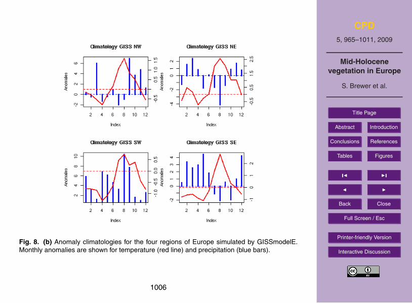
CPD5, 965–1011, 2009
Mid-Holocenevegetation in Europe
S. Brewer et al.
Title Page
Abstract Introduction
Conclusions References
Tables Figures
J I
J I
Back Close
Full Screen / Esc
Printer-friendly Version
Interactive Discussion
S. Brewer et al.: Mid-Holocene vegetation in Europe 9
Fig. 8a. Anomaly climatologies for the four regions of Europe sim-ulated by ECHAM5-MPIOM1. Monthly anomalies are shown fortemperature (red line) and precipitation (blue bars).
Fig. 8b. Anomaly climatologies for the four regions of Europe sim-ulated by GISSmodelE. Monthly anomalies are shown for tempera-ture (red line) and precipitation (blue bars).
calised warming, and the pattern of treeline shifts suggeststhat there was a land-sea gradient, with greater warming to-
Fig. 8c. Anomaly climatologies for the four regions of Europe sim-ulated by IPSL-CM4-V1-MR. Monthly anomalies are shown fortemperature (red line) and precipitation (blue bars).
Fig. 8d. Anomaly climatologies for the four regions of Europe sim-ulated by UBRIS-HadCM3M2. Monthly anomalies are shown fortemperature (red line) and precipitation (blue bars).
ward the continental interior. This is consistent with recon-420
structed warmer winter temperatures in the east of Europe
Fig. 8. (b) Anomaly climatologies for the four regions of Europe simulated by GISSmodelE.Monthly anomalies are shown for temperature (red line) and precipitation (blue bars).
1006
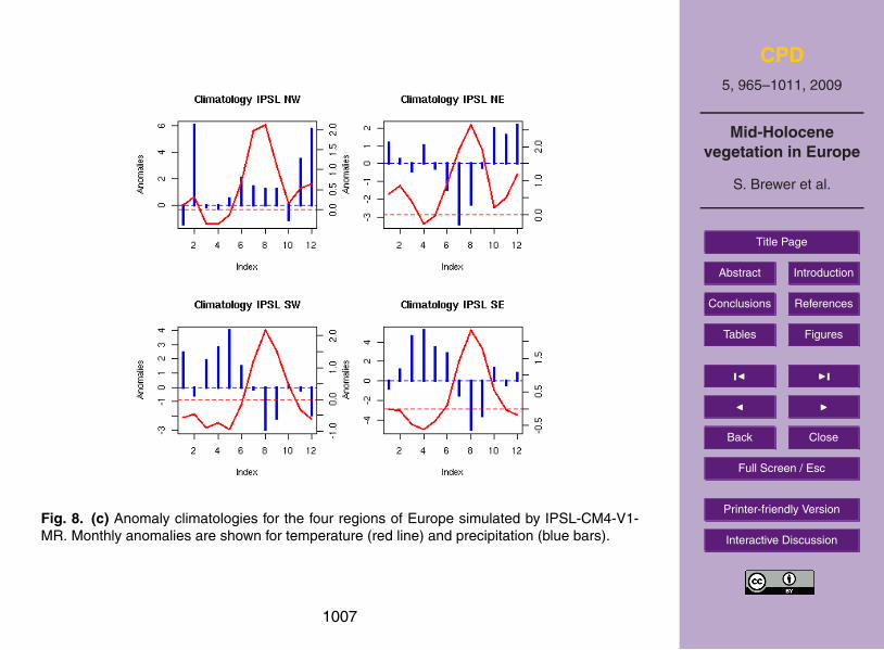
CPD5, 965–1011, 2009
Mid-Holocenevegetation in Europe
S. Brewer et al.
Title Page
Abstract Introduction
Conclusions References
Tables Figures
J I
J I
Back Close
Full Screen / Esc
Printer-friendly Version
Interactive Discussion
S. Brewer et al.: Mid-Holocene vegetation in Europe 9
Fig. 8a. Anomaly climatologies for the four regions of Europe sim-ulated by ECHAM5-MPIOM1. Monthly anomalies are shown fortemperature (red line) and precipitation (blue bars).
Fig. 8b. Anomaly climatologies for the four regions of Europe sim-ulated by GISSmodelE. Monthly anomalies are shown for tempera-ture (red line) and precipitation (blue bars).
calised warming, and the pattern of treeline shifts suggeststhat there was a land-sea gradient, with greater warming to-
Fig. 8c. Anomaly climatologies for the four regions of Europe sim-ulated by IPSL-CM4-V1-MR. Monthly anomalies are shown fortemperature (red line) and precipitation (blue bars).
Fig. 8d. Anomaly climatologies for the four regions of Europe sim-ulated by UBRIS-HadCM3M2. Monthly anomalies are shown fortemperature (red line) and precipitation (blue bars).
ward the continental interior. This is consistent with recon-420
structed warmer winter temperatures in the east of Europe
Fig. 8. (c) Anomaly climatologies for the four regions of Europe simulated by IPSL-CM4-V1-MR. Monthly anomalies are shown for temperature (red line) and precipitation (blue bars).
1007
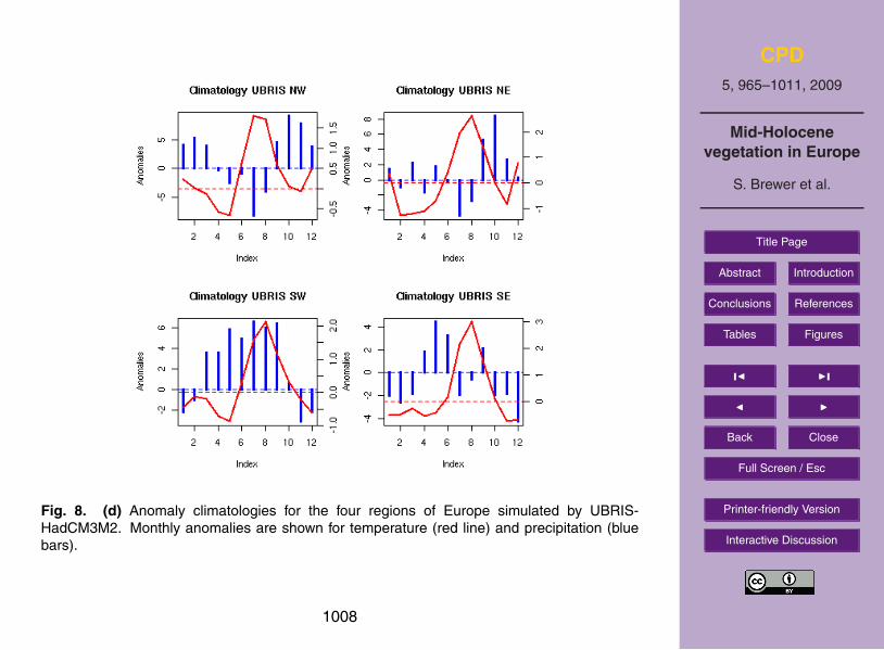
CPD5, 965–1011, 2009
Mid-Holocenevegetation in Europe
S. Brewer et al.
Title Page
Abstract Introduction
Conclusions References
Tables Figures
J I
J I
Back Close
Full Screen / Esc
Printer-friendly Version
Interactive Discussion
S. Brewer et al.: Mid-Holocene vegetation in Europe 9
Fig. 8a. Anomaly climatologies for the four regions of Europe sim-ulated by ECHAM5-MPIOM1. Monthly anomalies are shown fortemperature (red line) and precipitation (blue bars).
Fig. 8b. Anomaly climatologies for the four regions of Europe sim-ulated by GISSmodelE. Monthly anomalies are shown for tempera-ture (red line) and precipitation (blue bars).
calised warming, and the pattern of treeline shifts suggeststhat there was a land-sea gradient, with greater warming to-
Fig. 8c. Anomaly climatologies for the four regions of Europe sim-ulated by IPSL-CM4-V1-MR. Monthly anomalies are shown fortemperature (red line) and precipitation (blue bars).
Fig. 8d. Anomaly climatologies for the four regions of Europe sim-ulated by UBRIS-HadCM3M2. Monthly anomalies are shown fortemperature (red line) and precipitation (blue bars).
ward the continental interior. This is consistent with recon-420
structed warmer winter temperatures in the east of Europe
Fig. 8. (d) Anomaly climatologies for the four regions of Europe simulated by UBRIS-HadCM3M2. Monthly anomalies are shown for temperature (red line) and precipitation (bluebars).
1008
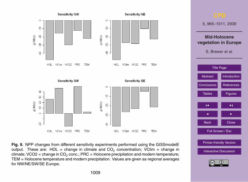
CPD5, 965–1011, 2009
Mid-Holocenevegetation in Europe
S. Brewer et al.
Title Page
Abstract Introduction
Conclusions References
Tables Figures
J I
J I
Back Close
Full Screen / Esc
Printer-friendly Version
Interactive Discussion
10 S. Brewer et al.: Mid-Holocene vegetation in Europe
(Davis et al., 2003). Precipitation changes in the north showno obvious pattern with a mixture of positive and negativeanomalies. One exception to this is the ECHAM5-MPIOM1simulation, which shows a general increase in precipitation425
throughout the year.In the south, changes in precipitation appear to play the
most important role. An increase in summer precipitation isseen in both models (GISSmodelE, HadCM3M2) that showthe same type of vegetation change as in the data, i.e. to-430
wards greater forest cover in the south-west (figures 8b and8d). The GISSmodelE also shows a general cooling through-out the year, with a much smaller summer increase than theother models, suggesting that temperature change may alsohave helped drive the vegetation changes. In the south-east,435
an increase in precipitation is simulated by the ECHAM5-MPIOM1 model throughout the majority of the year, and thisis the only model to not show an expansion of steppe vegeta-tion in this region.
In terms of parameters that control the distribution of440
plants more directly, these changes translate into an increasein soil water availability (figure 5) and a decrease in GDD5(figure 6). However, while all models show an increasein soil water in the Iberian peninsula, that covers a greateror lesser spatial area, an expansion of forest types is not445
seen in all simulations. This supports the role of tempera-ture changes in the mid-Holocene vegetation, in particular amarked lowering of GDD5. This change is of interest, as itshows that this variable is controlled by winter temperaturechanges in the south of Europe, and a reduction may occur,450
even when the summer temperature increases.The results show a general decline in NPP for the mid-
Holocene across Europe (table 3), with regional variations(figure 7). This fits with the slight decline in mid-Holoceneglobal NPP described by Beerling and Woodward (2001), us-455
ing two GCMs, although the variations given by these au-thors for the European latitudes are very close to modernvalues. However, the results obtained by Peng et al. (1998),using a statistical modelling approach based on pollen data,show an increase in NPP for this period. This second study460
does not explicitly model the photosynthetic process, anddoes not take into account the small change in atmosphericCO2 concentration at the mid-Holocene.
From the sensitivity experiments (figure 9), it is possibleto attribute the decline in NPP in the east of Europe to both465
changes in climate (VClim) and CO2 (VCO2) concentra-tion. Equally, while winter temperature played an importantrole in changing the composition of the forests in the north-east (Prentice), and water availability in the south-east (Pren-tice again), experiments with modern temperature (VPRC)470
or modern precipitation (VTEM) indicate that productivityin these regions was affected by changes in both these vari-ables.
In the north-west, changing CO2 concentration alone re-sults in a decrease of NPP equal to approximately 50% of475
the combined climate and CO2 effect. In contrast, when CO2
Fig. 9. NPP changes from different sensitivity experiments per-formed using the GISSmodelE output. These are: a) HOL = changein climate and CO2 concentration; b) VClim = change in climate;c) VCO2 = change in CO2 conc.; d) PRC = Holocene precipita-tion and modern temperature; e) TEM = Holocene temperature andmodern precipitation. Values are given as regional averages forNW/NE/SW/SE Europe.
is kept at modern levels and climate changed, this reductionis much smaller. This may be due to a strong gradient ofclimate anomalies in this region. Holding precipitation ortemperature to modern values causes a similar reduction, al-480
though the mid-Holocene temperatures have cause a largerchange when compared to modern values. Productivity in-creases in the south-west during the mid-Holocene. The sen-sitivity experiments suggest that this increase comes from theclimate change, offset by a reduction due to lower CO2 con-485
centration. Changing precipitation appears to account for allof the climatically induced NPP changes, whereas tempera-ture has little effect.
In general, the change due to CO2 concentration variationis relatively high, matching the effect of climate change in490
east of Europe. However, these changes are small, and fur-ther work will be necessary to test the sensitivity of CARAIBto CO2.
Bonfils et al. (2004) proposed a scenario of circulationchanges to explain the observed mid-Holocene winter cli-495
mate in Europe. We examine here whether the GCM pro-viding the best fit to the data in this study (GISSmodelE)supports this. The scenario is based on the existence of ananomalous low pressure system located over north-west Eu-rope causing an increased westerly flow over the south-west500
Fig. 9. NPP changes from different sensitivity experiments performed using the GISSmodelEoutput. These are: HOL = change in climate and CO2 concentration; VClim = change inclimate; VCO2 = change in CO2 conc.; PRC = Holocene precipitation and modern temperature;TEM = Holocene temperature and modern precipitation. Values are given as regional averagesfor NW/NE/SW/SE Europe.
1009
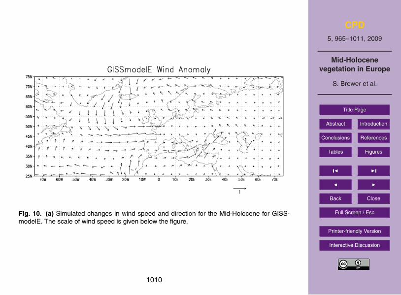
CPD5, 965–1011, 2009
Mid-Holocenevegetation in Europe
S. Brewer et al.
Title Page
Abstract Introduction
Conclusions References
Tables Figures
J I
J I
Back Close
Full Screen / Esc
Printer-friendly Version
Interactive Discussion
S. Brewer et al.: Mid-Holocene vegetation in Europe 11
Fig. 10a. Simulated changes in wind speed and direction for theMid-Holocene for GISSmodelE. The scale of wind speed is givenbelow the figure.
Fig. 10b. Simulated changes in wind speed and direction for theMid-Holocene for IPSL-CM4-V1-MR. The scale of wind speed isgiven below the figure.
and bringing moisture into the Mediterranean basin. Anyheating from the advection of these air masses was offsetby the reduction in insolation (Bonfils, 2001; Bonfils et al.,2004). Having lost moisture, the air masses then flowed northwere the smaller insolation anomalies were no longer suffi-505
cient to prevent warming.Changes in surface wind from the GISSmodelE simula-
tion, which provided the best fit to the data, support thisscenario (figure 10a), with a clear counter-clockwise and in-creased westerly flow over the Mediterranean. This is, how-510
ever, slightly displaced to the north and west compared toBonfils et al. (2004), and this may have limited the advec-tion of moisture towards the interior, resulting in the reducedmoisture availability in south eastern Europe. A similar pat-tern can be seen in both the HadCM3M2 and ECHAM5-515
MPIOM GCMs, but in both cases, the area of low pressureis positioned further to the north-west. This limits the west-erly flow in the HadCM3M2 model and results in a moresoutherly flow in the ECHAM5-MPIOM. This pattern ap-pears to be absent in the IPSL-CM4-V1-MR wind patterns520
(figure 10b).
5 Conclusions
– Simulated vegetation distributions based on coupledocean-atmosphere GCMs show a poleward shift inFennoscandia, with a corresponding loss of tundra and525
boreal montane forest, that are consistent with the ob-served changes.
– In central Europe there is a change in forest compositionin central European forests toward a dominance of cooltemperate forest types.530
– The observed southward spread of temperate forests isnot observed in any model, but two simulations show anincrease in forest cover, with loss of desert, semi-desertand temperate grasslands.
– Changes in the south are driven by increased moisture535
availability, but lower winter temperatures also playeda role. In the Mediterranean region, a decrease in therelatively higher winter temperatures leads to a decreasein GDD5, which may be reconstructed as lower summertemperatures.540
– The observed pattern of changes is consistent with in-creased westerly flow from Atlantic, bringing increasedprecipitation over the Mediterranean basin.
Acknowledgements. Financial support for the study was providedby FRFC convention no. 2.4555.06. The work forms part of545
project DECVEG from the European Science Foundation (ESF)under the EUROCORES Programme EuroCLIMATE, throughcontract No. ERAS-CT-2003-980409 of the European Com-mission, DG Research, FP6. We thank the PMIP2 Database(http://pmip2.lsce.ipsl.fr/) for providing GCM data.550
References
Beerling, D. and Woodward, F.: Vegetation and the Terrestrial Car-bon Cycle: Modelling the First 400 Million Years, CambridgeUniversity Press, 2001.
Berger, A.: Long-term variations of daily insolation and Quaternary555
climatic changes, Journal of Atmospheric Sciences, 35, 2362–2367, 1978.
Bonfils, C.: Le moyen-Holocene: role de la surface continentale surla sensibilite climatique simulee, Ph.D. thesis, Universite ParisVI, Paris, 322 pp., 2001.560
Bonfils, C., de Noblet-Ducoudre, N., Guiot, J., and Bartlein, P. J.:Some mechanisms of mid-Holocene climate change in Europe,inferred from comparing PMIP models to data, Climate Dynam-ics, 23, 79–98, 2004.
Braconnot, P., Otto-Bliesner, B., Harrison, S., Joussaume, S., Pe-565
terchmitt, J.-Y., Abe-Ouchi, A., Crucifix, M., Driesschaert, E.,Fichefet, T., Hewitt, C. D., Kageyama, M., Kitoh, A., Laıne, A.,Loutre, M.-F., Marti, O., Merkel, U., Ramstein, G., Valdes, P.,Weber, S. L., Yu, Y., and Zhao, Y.: Results of PMIP2 coupledsimulations of the Mid-Holocene and Last Glacial Maximum -570
Part 1: experiments and large-scale features, Climate of the Past,3, 261–277, 2007.
Fig. 10. (a) Simulated changes in wind speed and direction for the Mid-Holocene for GISS-modelE. The scale of wind speed is given below the figure.
1010
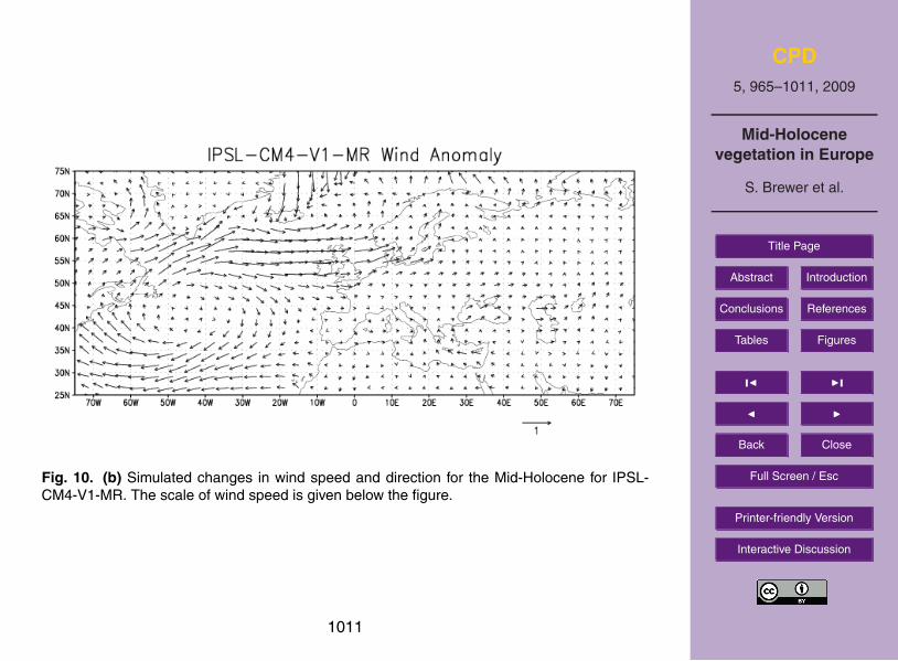
CPD5, 965–1011, 2009
Mid-Holocenevegetation in Europe
S. Brewer et al.
Title Page
Abstract Introduction
Conclusions References
Tables Figures
J I
J I
Back Close
Full Screen / Esc
Printer-friendly Version
Interactive Discussion
S. Brewer et al.: Mid-Holocene vegetation in Europe 11
Fig. 10a. Simulated changes in wind speed and direction for theMid-Holocene for GISSmodelE. The scale of wind speed is givenbelow the figure.
Fig. 10b. Simulated changes in wind speed and direction for theMid-Holocene for IPSL-CM4-V1-MR. The scale of wind speed isgiven below the figure.
and bringing moisture into the Mediterranean basin. Anyheating from the advection of these air masses was offsetby the reduction in insolation (Bonfils, 2001; Bonfils et al.,2004). Having lost moisture, the air masses then flowed northwere the smaller insolation anomalies were no longer suffi-505
cient to prevent warming.Changes in surface wind from the GISSmodelE simula-
tion, which provided the best fit to the data, support thisscenario (figure 10a), with a clear counter-clockwise and in-creased westerly flow over the Mediterranean. This is, how-510
ever, slightly displaced to the north and west compared toBonfils et al. (2004), and this may have limited the advec-tion of moisture towards the interior, resulting in the reducedmoisture availability in south eastern Europe. A similar pat-tern can be seen in both the HadCM3M2 and ECHAM5-515
MPIOM GCMs, but in both cases, the area of low pressureis positioned further to the north-west. This limits the west-erly flow in the HadCM3M2 model and results in a moresoutherly flow in the ECHAM5-MPIOM. This pattern ap-pears to be absent in the IPSL-CM4-V1-MR wind patterns520
(figure 10b).
5 Conclusions
– Simulated vegetation distributions based on coupledocean-atmosphere GCMs show a poleward shift inFennoscandia, with a corresponding loss of tundra and525
boreal montane forest, that are consistent with the ob-served changes.
– In central Europe there is a change in forest compositionin central European forests toward a dominance of cooltemperate forest types.530
– The observed southward spread of temperate forests isnot observed in any model, but two simulations show anincrease in forest cover, with loss of desert, semi-desertand temperate grasslands.
– Changes in the south are driven by increased moisture535
availability, but lower winter temperatures also playeda role. In the Mediterranean region, a decrease in therelatively higher winter temperatures leads to a decreasein GDD5, which may be reconstructed as lower summertemperatures.540
– The observed pattern of changes is consistent with in-creased westerly flow from Atlantic, bringing increasedprecipitation over the Mediterranean basin.
Acknowledgements. Financial support for the study was providedby FRFC convention no. 2.4555.06. The work forms part of545
project DECVEG from the European Science Foundation (ESF)under the EUROCORES Programme EuroCLIMATE, throughcontract No. ERAS-CT-2003-980409 of the European Com-mission, DG Research, FP6. We thank the PMIP2 Database(http://pmip2.lsce.ipsl.fr/) for providing GCM data.550
References
Beerling, D. and Woodward, F.: Vegetation and the Terrestrial Car-bon Cycle: Modelling the First 400 Million Years, CambridgeUniversity Press, 2001.
Berger, A.: Long-term variations of daily insolation and Quaternary555
climatic changes, Journal of Atmospheric Sciences, 35, 2362–2367, 1978.
Bonfils, C.: Le moyen-Holocene: role de la surface continentale surla sensibilite climatique simulee, Ph.D. thesis, Universite ParisVI, Paris, 322 pp., 2001.560
Bonfils, C., de Noblet-Ducoudre, N., Guiot, J., and Bartlein, P. J.:Some mechanisms of mid-Holocene climate change in Europe,inferred from comparing PMIP models to data, Climate Dynam-ics, 23, 79–98, 2004.
Braconnot, P., Otto-Bliesner, B., Harrison, S., Joussaume, S., Pe-565
terchmitt, J.-Y., Abe-Ouchi, A., Crucifix, M., Driesschaert, E.,Fichefet, T., Hewitt, C. D., Kageyama, M., Kitoh, A., Laıne, A.,Loutre, M.-F., Marti, O., Merkel, U., Ramstein, G., Valdes, P.,Weber, S. L., Yu, Y., and Zhao, Y.: Results of PMIP2 coupledsimulations of the Mid-Holocene and Last Glacial Maximum -570
Part 1: experiments and large-scale features, Climate of the Past,3, 261–277, 2007.
Fig. 10. (b) Simulated changes in wind speed and direction for the Mid-Holocene for IPSL-CM4-V1-MR. The scale of wind speed is given below the figure.
1011