mid-latitude cyclones south of africa in the genesis gcm

INTERNATIONAL JOURNAL OF CLIMATOLOGY, VOL. 17, 459–473 (1997)

MID-LATITUDE CYCLONES SOUTH OF AFRICA IN THE GENESIS GCM

D. A. HUDSON* AND B. C. HEWITSON

Department of Environmental and Geographical Science, University of Cape Town, Private Bag, Rondebosch, Cape Town, 7701, South Africaemail: [email protected]

Received 19 July 1995Revised 20 September 1996

Accepted 20 September 1996

ABSTRACT

This paper examines the density, distribution and characteristics of mid-latitude cyclones in the oceans south of Africa in theGENESIS general circulation model (GCM). The latest version of the GENESIS GCM (version 2.0.a), as well as itspredecessor (version 1.02), are evaluated to assess whether version 2.0.a is an improvement over version 1.02 in terms of mid-latitude cyclones. An automated cyclone finding program was used to identify cyclone centres. This program was applied to 5years of twice daily GENESIS (versions 1.02 and 2.0.a) sea-level pressure data, as well as to 10 years of a gridded assimilationof observed data for the winter season (June, July, August).

The results show that version 1.02 does not simulate the full meridional sea-level pressure range over the analysis window,whereas version 2.0.a is closer to that of the observed data. The circumpolar trough in version 1.02 is between 10 and 15 hPatoo weak and it extends too far equatorward. The trough is captured better by version 2.0.a, probably due to its finer gridresolution (T31) compared with that of version 1.02 (R15 resolution). In both versions, cyclone densities north of 55�S arehigher than observed and the high cyclone density band around the pole in version 1.02 is poorly defined. Discrepanciesbetween the two versions, and the model and observed data, have been related to factors such as grid resolutions, topography,heat transport and sea-ice extent. Version 1.02 does not simulate the full meridional gradient of cyclone central pressures,whereas version 2.0.a is a better representation of the observed data. Both versions exhibit greater variability in the sea-levelpressure field compared with the observed data. GENESIS version 2.0.a is a considerable improvement over its predecessor interms of mid-latitude cyclones in the African region of the southern oceans.#1997 by the Royal Meteorological Society. Int.J. Climatol. 17: 459–473, 1997.

(No. of Figs: 8. No. of Tables: 0. No. of Refs: 45.)

KEY WORDS: southern Africa; Southern Ocean; general circulation models; GENESIS model; mid-latitude cyclones.

INTRODUCTION

The National Centre for Atmospheric Research’s (NCAR) GENESIS (Global Environmental and EcologicalSimulation of Interactive Systems) model originated out of an effort to develop a first-generation earth systemmodel which especially emphasizes terrestrial physical, biophysical and cryospheric processes (Thompson andPollard, 1995, 1997). This general circulation model (GCM) has been widely used by climatologists and hasfound a particular niche in palaeoclimate modelling (Barronet al., 1993, 1995; Crowleyet al., 1993, 1996; Otto-Bliesner, 1993; Crowley and Baum, 1994; Foley, 1994; Jenkins, 1995). However, comparatively little effort hasbeen devoted to evaluating the model’s simulation of the present climate, particularly of the SouthernHemisphere. Validation studies play an important role in facilitating the improvement of GCMs and they providea perspective on the limitations of the model, which need to be taken into consideration when performing pastand future climate simulations. The primary purpose of this paper is to examine the density, distribution and

CCC 0899-8418/97/050459-16 $17.50# 1997 by the Royal Meteorological Society

*Correspondence to: D. A. Hudson

Contract grant sponsor: Foundation for Research Development, South Africa

characteristics of mid-latitude cyclones, south of South Africa, in GENESIS GCM data. At present, it has yet tobe shown whether mid-latitude cyclones are adequately simulated by the model.

Mid-latitude cyclones are vital for meridional energy transport in the Southern Hemisphere and it is thusimportant to study these transient disturbances in both observed and model data. Studies of Northern Hemispherecyclones date back to the 1800’s (e.g. Van Bebber, 1882). Unfortunately, Southern Hemisphere studies have beenrestricted by poor data coverage of the southern oceans (Murray and Simmonds, 1991a). Taljaard (1967) madethe first major contribution by producing hemispheric charts and analysing mid-latitude cyclone distributions forthe years 1957 and 1958. Subsequently, a number of studies making use of both daily weather charts (e.g. VanLoon, 1965) and satellite imagery (e.g. Streten and Troup, 1973; Carleton, 1979) have been undertaken. Themajority of Southern Hemisphere studies have been based on manual techniques with observed data. Theseschemes may have suffered from subjectivity and have the problem of being time consuming. It is only inrelatively recent times that the development of automated analyses have facilitated the rapid and objectiveidentification of cyclones from observed digital data as well as allowing the examination of mid-latitude cyclonesin model-generated data. These numerical analyses have been based on a number of different algorithms (e.g. LeMarshall and Kelly, 1981; Lambert, 1988; Le Treut and Kalnay, 1990; Murray and Simmonds, 1991a; Ko¨nig etal., 1993; Serrezeet al., 1993; Sinclair, 1994, 1995; Changnonet al., 1995).

In this study, an automated cyclone-finding program has been used and is based on the algorithm devised byMurray and Simmonds (1991a). Mid-latitude cyclones are identified by the existence of pronounced cyclonicvorticity maxima in the pressure field. Some of the salient features of the program are referred to in the followingsection.

The latest version of the GENESIS GCM (version 2.0.a) was released at the end of 1995. It has a finerresolution than its predecessor (version 1.02) and some new model physics have been incorporated. This paperwill determine overall cyclone validity and will compare the two versions of the model in order to evaluate theircapabilities and to assess whether version 2.0.a (hereafter referred to as version 2) is an improvement over version1.02 (hereafter referred to as version 1) in terms of mid-latitude cyclones in the African sector of the SouthernOcean.

DATA AND METHODS

The analyses are restricted to winter (JJA, i.e. June, July, August) and have been performed over a windowextending from 80�S to 25�S and from 45�W to 100�E. The Australian Southern Hemisphere gridded analyses ofsea-level pressure, produced by the Australian Bureau of Meteorology, have been used as the observational database for comparison with GCM data. The methods used to obtain this Southern Hemisphere sea-level pressuredata set have been documented by Le Marshallet al. (1985). Twice daily data for 10 winters (1979–1988) havebeen extracted. The data set is presented on a nominally equidistant 47647 polar stereographic grid, centred onthe South Pole, with an effective resolution of approximately 508 km at 60�S. The quality of the earlier years ofthe data set has been discussed by Trenberth (1979) and Swanson and Trenberth (1981) and used in a SouthernHemisphere cyclone analysis by Le Marshall and Kelly (1981). Jones and Simmonds (1993) used data from thelatter portion of the analyses (1975–1990) in order to produce their climatology of Southern Hemispherecyclones. The Australian gridded analyses of sea-level pressure will hereafter be referred to as the observed data.

Five years of data were available from the control simulations of both versions of GENESIS. Twice daily sea-level pressure data for JJA of these years were extracted for each version. Detailed descriptions of GENESISversion 1 and version 2 are provided by Thompson and Pollard (1995) and Thompson and Pollard (1997)respectively, but a few of the primary differences between the two versions are discussed below.

Both versions of GENESIS consist of an atmospheric general circulation model (AGCM) coupled to multilayermodels of vegetation, soil and land ice, snow, sea-ice, and a 50 m slab oceanic layer. Version 1 has an R15spectral resolution with 12 atmospheric levels, whereas version 2 has a T31 resolution with 18 atmosphericlevels. The surface models of both versions have a 2� by 2� resolution and fields are transferred between theAGCM and surface by bilinear interpolation or area-averaging at each time-step. The cloud scheme used in thetwo versions is significantly different. Version 1 uses a cloud parameterization, similar to that of Slingo and

460 D. A. HUDSON AND B. C. HEWITSON

Slingo (1991), with three possible cloud types (stratus, anvil cirrus and convective). In version 2, however, cloudsare predicted using prognostic three-dimensional cloud water amounts (e.g. Smith, 1990; Senior and Mitchell,1993). Separate prognostic cloud fields are kept for the three cloud types used in version 1 and they are mixedvertically by convection plumes and diffusion and are advected by semi-Lagrangian transport. Cloud conversionto precipitation, evaporation, aggregation by falling precipitation, re-evaporation of falling precipitation, andturbulent deposition of lowest-layer cloud particles onto the surface are all new additions in version 2.

The single-level cloud approximation related to solar radiation (Thompsonet al., 1987) has been removed inversion 2 and instead, delta-Eddington calculations are made for clear and cloudy fractions of each layer.Furthermore, additional cloud absorption of solar radiation (Cesset al., 1995; Ramanathanet al., 1995) has beenincluded in this more recent version. The convective plume model, used in version 1 (Thompson and Pollard,1995), has been tuned to provide better results in version 2 and the planetary boundary-layer plumes that aretriggered by surface fluxes can now condense and precipitate, whereas in version 1 they were always assumed tobe dry. Some other new features of version 2’s AGCM include gravity wave drag, radiative effects of prescribedtropospheric dust aerosols and the ability to prescribe uniform mixing ratios of individual greenhouse gases (CO2,CH4, N2O, CFC11 and CFC12). The vegetation, soil, snow, sea-ice and slab-ocean models also have some newfeatures incorporated in version 2 of GENESIS. These are discussed in detail by Thompson and Pollard (1997).

The cyclone-finding program was written in accordance with the algorithm presented in the paper by Murrayand Simmonds (1991a). The cyclone-tracking section of their algorithm has not been implemented. In theprogram, a bicubic spline function is applied to the gridded pressure field, on a 476 47 polar stereographic grid,so that the best estimate of the location of the low can be obtained. Identification of lows is performed on thisregular grid. For the GCM data, it was necessary to interpolate the data from a latitude–longitude grid to the polarstereographic grid. This was done by means of a spherical interpolation routine (Willmottet al., 1985). At thefirst stage of the program, the gridded pressure data is scanned in order to identify grid-points at which theLaplacian of the pressure,

H2p�xi; yj� � pxx � pyy;

is greater than at any of the eight surrounding grid-points and greater than a prescribed positive value. Theprescribed value used in this study was 4 hPa. These identified grid-points serve as starting points for an iterativedifferential routine, based on ellipsoidal minimization techniques, which is used to search for a pressureminimum (p). This pressure minimum corresponds to the position of a closed low (a system possessing a closedisobar at a certain interval). The algorithm of Murray and Simmonds (1991a) also allows for the inclusion of openlows (an inflexion in the pressure field, i.e. not possessing a closed isobar), however, this has not been included inthe current study because it was found, upon validation of the scheme, that closed-low identification wassufficient for identifying the major systems. In addition, the inclusion of open lows often meant that zones ofcurved isobars, not usually regarded as cyclones, tended to be included. Sinclair (1994), who used a cycloneidentification scheme based on the algorithm of Murray and Simmonds (1991a), also noted that the inclusion ofopen lows in his study sometimes resulted in the identification of certain zones of curvature and regions ofelongated geostrophic shear, which would not be identified as cyclones in manual analyses. As in the presentstudy, Toljaard (1967) also restricted cyclones to those systems possessing a closed isobar. In order to excludeheat lows and other small-scale and shallow features, a minimum average value ofH

2p over a specified radius ofthe cyclone centre was stipulated. This was obtained by calculatingH

2p at the eight compass points at a 0�5 grid-unit radius from the cyclone centre and also at a 1 grid-unit radius from the cyclone centre. The average of these17 points (including the cyclone centre) was then calculated (let the value� AVE) and evaluated according tothe following statement:

If AVE5 2 sinY� 4�5, then the low is accepted (Y is the absolute value of the degrees latitude)

This equation was obtained through a tuning process with the observed data, such that we felt that the majorsystems were being located and the more insignificant ones discarded. The cyclone-finding program wassometimes found to converge on the same low pressure from different starting points. In order to eliminate theproblem of finding two output positions very close together on the same day, a minimum cyclone separationdistance of 8� was imposed.

MID-LATITUDE CYCLONES SOUTH OF AFRICA IN THE GENESIS GCM 461

In this paper, cyclone densities refer to the average number of mid-latitude cyclones per degree (latitude)2 atany one time. As such, densities were normalized for area and the total number of time-steps investigated.Meridional profiles of mean sea-level pressure, cyclone densities (number of cyclones per (degree latitude)2) andcyclone central pressures were obtained by computing zonal means at latitude intervals defined by the T31 gridover the analysis window (i.e. 80�S to 25�S and 45�W to 100�E).

Time-averaged fields of JJA sea-level pressure are also displayed and analysed in order to aid interpretation ofthe mid-latitude cyclone results. In addition, the variance in the pressure field associated with mid-latitudecyclones is examined. In the Southern Hemisphere mid-latitudes, atmospheric variability on 2- to 8-daytimescales can largely be attributed to the passage of cyclones and anticyclones (Trenberth, 1991). As such, thestandard deviation of the bandpass filtered data was calculated and displayed in an attempt to identify majorstorm tracks. The bandpass filter of 1�5–8�5 days was used and was calculated by means of moving averages.Results are displayed on a polar stereographic projection.

RESULTS AND DISCUSSION

Sea-level pressure

The time-averaged sea-level pressure provides the background against which cyclones are formed and is, inturn, affected by the incidence of cyclones. Figure 1 shows the average JJA sea-level pressure for the observeddata and versions 1 and 2 of GENESIS. The region of the subtropical high-pressure cells (pressures greater than1020 hPa) is apparent at about 30�S in the observed data (Figure 1(a)), with pressures then decreasing to aminimum of about 980 hPa around 65�S, coincident with the circumpolar trough. It is evident from Figure 1(b)that the model-generated (version 1) sea-level pressures are too low in the region between 30� and 35�S and thesubtropical high-pressure cells are not well defined. Furthermore, the meridional pressure gradient over theanalysis window is too weak (Figure 1(b)) in comparison with the observed data (Figure 1(a)) and, subsequently,pressures from version 1 only reach minima of about 1000 hPa around Antarctica. As such, the circumpolartrough is not deep enough in version 1 and it extends too far equatorward. In contrast, version 2 (Figure 1(c))performs better than version 1 in terms of sea-level pressure. It is clear from Figure 2, showing the JJA zonallyaveraged (over the analysis window) sea-level pressure, that the meridional pressure gradient simulated byversion 2 is closer to that of the observed data, in comparison with the pressure gradient obtained from version 1.In Thompson and Pollard’s (1995) validation of version 1 of GENESIS they remarked that the R15 resolution ofthe model meant that there was poor resolution of Hadley Cell dynamics and that many sea-level pressurefeatures were indistinct. The improvement in the simulation of sea-level pressure in version 2 can probably beattributed to the finer resolution (T31) of the AGCM.

It does seem, however, that pressures are shifted slightly north in version 2 when compared with the observeddata (Figures 1 and 2). Figure 2 shows that the minimum pressure associated with the circumpolar trough occursat about 61�S in version 2 and at 65�S in the observed data. In addition, the spatial extent of the subtropical high-pressure cells in version 2 (Figure 1(c)) is far less than the observed.

In both versions of GENESIS, pressures over the Antarctic continent are too high compared with the observeddata. This is a common problem with many GCM simulations and may be due to insufficient resolution to dealwith the dynamical effects of the steep Antarctic topography (Bromwichet al., 1995; Thompson and Pollard,1997).

Cyclone densities

Cyclone densities obtained from the observed data are displayed on Figure 3(a). The pattern and magnitude ofthe densities are comparable with those obtained by Jones and Simmonds (1993), although values in the presentstudy are marginally lower. This is most likely due to inclusion of open lows in their study. The high-density corearound the Antarctic continent, consistent with other manual and automated analyses of mid-latitude cyclones(Taljaard, 1967; Le Marshall and Kelly, 1981; Jones and Simmonds, 1993), is associated with the circumpolartrough. Taljaard (1967) found that cyclone centres are most numerous 2–6� equatorward of the hemispheric mean


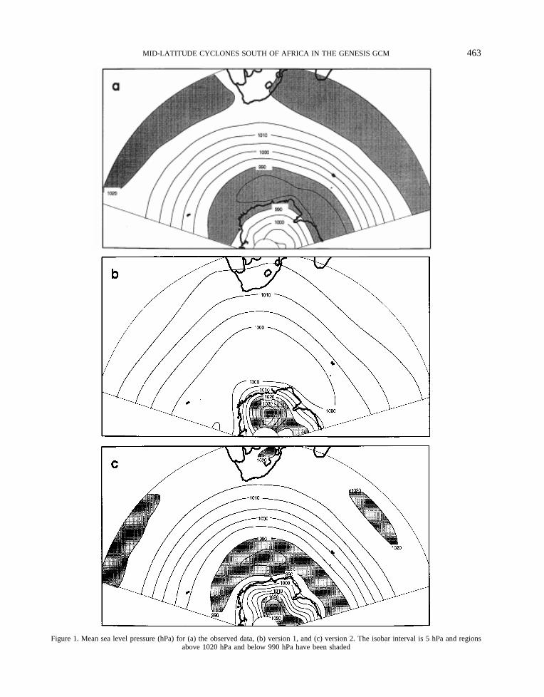
Figure 1. Mean sea level pressure (hPa) for (a) the observed data, (b) version 1, and (c) version 2. The isobar interval is 5 hPa and regionsabove 1020 hPa and below 990 hPa have been shaded


position of the circumpolar trough. From the zonally averaged sea-level pressure (Figure 2) and cyclone densities(Figure 4) it is evident that the circumpolar trough (in the analysis window) is centred around 65�S and thatcyclone densities peak at about 26 1073 cyclones per (degree latitude)2 near 61�S.

In manual analyses done by Kep (1984), he noted a general tendency for cyclones to form preferentiallybetween 40�S and 50�S during July, and Jones and Simmonds (1993) found a subsidiary cyclone maximum at40�S. This maximum is evident on the meridional profile of cyclone densities (Figure 4), where there is a smallpeak at about 40�S in the observed data. The region that contributes most to this peak lies west of 20�E in theanalysis window (Figure 3(a)). This zone of cyclone activity has been referred to as a ‘spiral arm’ which stretchesfrom the Gran Chaco cyclogenetic area of South America in a south-easterly direction across the Atlantic tomerge with the high density circumpolar core south of Africa (Taljaard, 1967).

It is evident from Figure 3(b) that version 1 of GENESIS overestimates cyclone activity. The magnitude of thepeak densities are not beyond values recorded in the observed data (Figure 3(a)), but cyclone activity is spreadover a broad band in the analysis window instead of occupying a narrow region in association with thecircumpolar trough. From the meridional profile of cyclone densities for version 1 (Figure 4), it is clear thatzonally averaged densities do peak near 61�S, as in the observed data, but that densities are too low in this regionand are too high between 55� and 35�S.

Version 2 of GENESIS captures the pattern of cyclone densities better than version 1. The zonally averagedpeak density (Figure 4) corresponds to that of the observed data, but the distribution around the peak is stillslightly skewed. There are too few cyclones south of 61�S and too many north of this latitude. The high densitycircumpolar band is better defined in version 2 compared with version 1 (Figure 3) and the magnitude of thiscyclone density peak near 61�S is more realistic (Figure 4). These differences are all related, in part, to theimproved simulation of the circumpolar trough in version 2 (Figure 1).

Most of the improvements in the pattern and magnitude of cyclone densities from version 1 to version 2 canprobably be attributed to the finer AGCM grid in version 2. Many cyclones may be too small to be resolved bythe R15 resolution of version 1. This could partially explain why cyclone densities south of about 58�S are less inversion 1 compared with both version 2 and the observed data (Figure 4). South of 55�S, mesocyclones (also

Figure 2. Zonally averaged (45�W to 100�E) mean sea-level pressure (hPa) for the observed data, version 1 and version 2


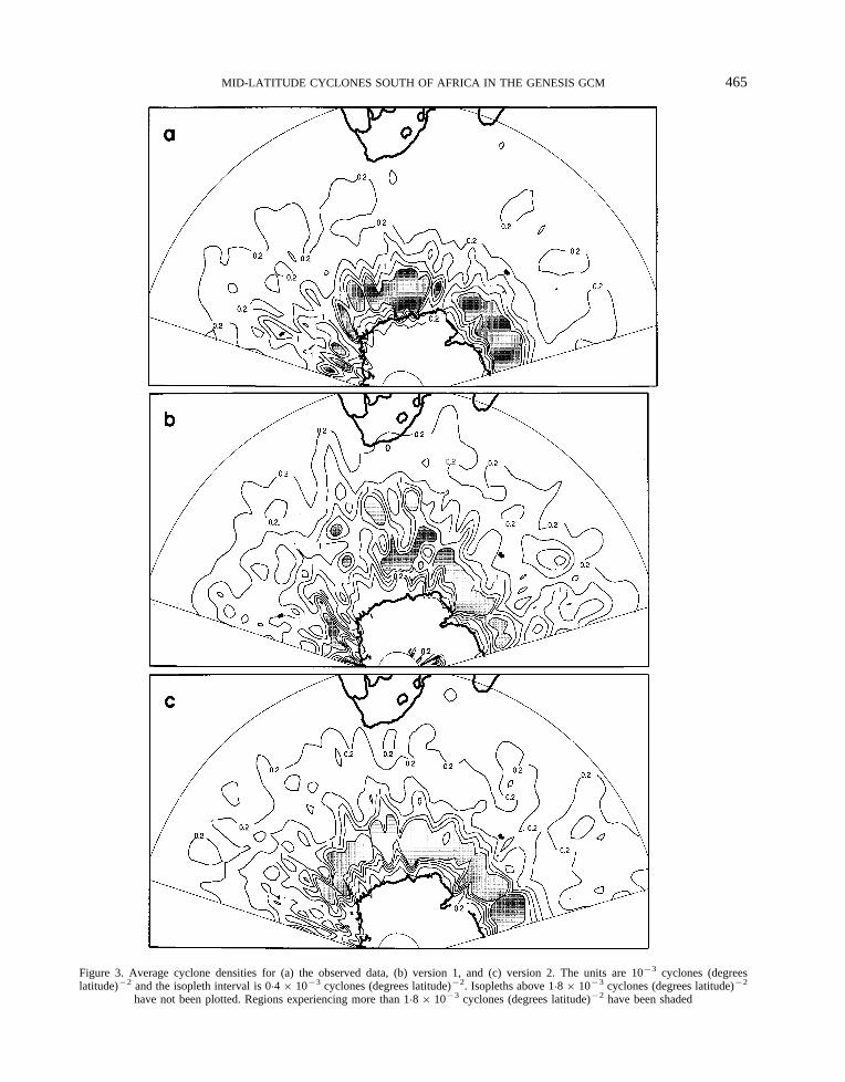
Figure 3. Average cyclone densities for (a) the observed data, (b) version 1, and (c) version 2. The units are 1073 cyclones (degreeslatitude)72 and the isopleth interval is 0�461073 cyclones (degrees latitude)72. Isopleths above 1�861073 cyclones (degrees latitude)72

have not been plotted. Regions experiencing more than 1�861073 cyclones (degrees latitude)72 have been shaded


referred to as polar lows) are more common than the larger ‘synoptic’ (frontal) cyclones (Carleton and Carpenter,1990). These mesocyclones may constitute up to 50 per cent of all cyclones recorded during winter over theSouthern Hemisphere oceans (Carleton, 1995). Mesocyclones are vortices that develop in cold air streams andhave average diameters of about 375 km (� 3�4�), compared with the larger synoptic cyclones which havediameters around 1035 km (� 9�3�) (Carleton, 1995). As such, the mesocyclones may not be detected by version1, whose AGCM resolution translates to about 4�5� latitude by 7�5� longitude, whereas version 2 has an effectiveresolution of about 3�7� latitude by 3�75� longitude, and there is thus a greater probability that mesocyclones willbe recorded. The observed data set, presented on a nominally equidistant polar sterographic grid, has a resolutionof about 4�5� latitude by 4�5� longitude in the mid-latitudes, thus being a coarser grid than GENESIS version 2.This may, in part, contribute to the higher density of cyclones recorded by version 2 north of 62�S (Figure 4),where smaller scale cyclones are resolved in the model, but not in the observed data.

In addition, as was discussed earlier, the circumpolar trough in version 1 (Figure 1(b) and Figure 2) extends toofar equatorward, probably due to the coarse resolution of the AGCM being unable to simulate the steepmeridional pressure gradients, and this could be related to the anomalously broad band of cyclone activity (65�S–40�S) that extends across the analysis window (Figure 3(b)).

It is unlikely that all the differences, described thus far, between the two versions are solely due to the changein resolution (both horizontal and vertical). Modified model physics and parameterizations are also likely to haveimpacted on the simulation of cyclones. Thompson and Pollard (1995) looked at patterns of vertical velocities inversion 1 of GENESIS and observed that the model captured the strength and position of the Ferrel and HadleyCells fairly well, except for an incorrect ascending region around 40�S during July. This could be related to theanomalously high number of cyclones observed in this region (Figure 3(b) and Figure 4). The incorrect ascendingregion may be due to an overly active convective plume scheme in the model (Thompson and Pollard, 1995) andthis scheme has been modified and adjusted in version 2 to provide better results.

Furthermore, oceanic heat transport in version 2 is different from version 1. In version 1, convergence isprescribed as a function of latitude, whereas in version 2 the present-day observed zonal mean transport is fitted

Figure 4. Zonally averaged (45�W to 100�E) cyclone densities (1073 cyclones (degrees latitude)72) for the observed data, version 1 andversion 2


as a linear function of the latitudinal sea-surface temperature gradient, with the diffusion coefficient dependent onlatitude and the zonal fraction of land versus ocean (Thompson and Pollard, 1997). Thompson and Pollard (1995)note that in version 1 there is too much horizontal heat transport to higher latitudes and that this is probably due toboth the coarse AGCM resolution and the simplistic prescription of heat transport, especially south of 60�S. Thismay be related to the large number of cyclones between 35� and 55�S (Figure 3(b) and Figure 4). An importantregion of cyclogenesis for frontal cyclones in the analysis window is situated off the east coast of South America(Taljaard, 1967; Sinclair, 1995), apparently linked to the warm Brazil ocean current (Sinclair, 1995). Withanomalously high heat transport in version 1 of GENESIS, it is likely that the magnitude of the warm water inthis region is overestimated, possibly leading to enhanced energy input into the atmosphere and thus potentiallymore cyclogenesis.

Another improvement of version 2 over its predecessor is better data input files for the land–ocean–ice-sheetmask, topography, and open water fraction, which were obtained using the 10 minute U.S. Navy FNOC globalelevation data set (Cuming and Hawkins, 1981; Kineman, 1985) and Cogley’s 1� by 1� data sets for ice-sheets(Cogley, 1991). A better representation of topography in version 2 may have helped to produce a more realisticcyclone density field, because topography influences lee cyclogenesis east of the Andes, near 45�S (Jones andSimmonds, 1993; Sinclair, 1995), and Antarctic topography may be important for local cyclogenesis over thesteep Antarctic slopes, as well as having an influence on the distribution of cyclolysis around the Antarcticcoastline (Sinclair, 1994).

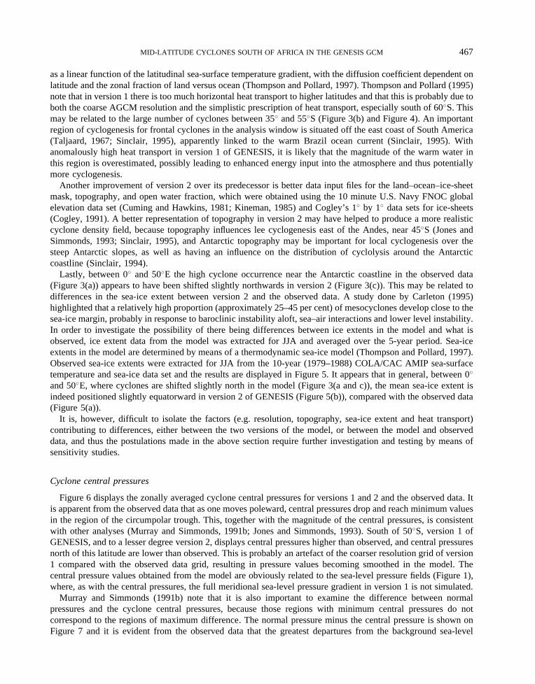
Lastly, between 0� and 50�E the high cyclone occurrence near the Antarctic coastline in the observed data(Figure 3(a)) appears to have been shifted slightly northwards in version 2 (Figure 3(c)). This may be related todifferences in the sea-ice extent between version 2 and the observed data. A study done by Carleton (1995)highlighted that a relatively high proportion (approximately 25–45 per cent) of mesocyclones develop close to thesea-ice margin, probably in response to baroclinic instability aloft, sea–air interactions and lower level instability.In order to investigate the possibility of there being differences between ice extents in the model and what isobserved, ice extent data from the model was extracted for JJA and averaged over the 5-year period. Sea-iceextents in the model are determined by means of a thermodynamic sea-ice model (Thompson and Pollard, 1997).Observed sea-ice extents were extracted for JJA from the 10-year (1979–1988) COLA/CAC AMIP sea-surfacetemperature and sea-ice data set and the results are displayed in Figure 5. It appears that in general, between 0�

and 50�E, where cyclones are shifted slightly north in the model (Figure 3(a and c)), the mean sea-ice extent isindeed positioned slightly equatorward in version 2 of GENESIS (Figure 5(b)), compared with the observed data(Figure 5(a)).

It is, however, difficult to isolate the factors (e.g. resolution, topography, sea-ice extent and heat transport)contributing to differences, either between the two versions of the model, or between the model and observeddata, and thus the postulations made in the above section require further investigation and testing by means ofsensitivity studies.

Cyclone central pressures

Figure 6 displays the zonally averaged cyclone central pressures for versions 1 and 2 and the observed data. Itis apparent from the observed data that as one moves poleward, central pressures drop and reach minimum valuesin the region of the circumpolar trough. This, together with the magnitude of the central pressures, is consistentwith other analyses (Murray and Simmonds, 1991b; Jones and Simmonds, 1993). South of 50�S, version 1 ofGENESIS, and to a lesser degree version 2, displays central pressures higher than observed, and central pressuresnorth of this latitude are lower than observed. This is probably an artefact of the coarser resolution grid of version1 compared with the observed data grid, resulting in pressure values becoming smoothed in the model. Thecentral pressure values obtained from the model are obviously related to the sea-level pressure fields (Figure 1),where, as with the central pressures, the full meridional sea-level pressure gradient in version 1 is not simulated.

Murray and Simmonds (1991b) note that it is also important to examine the difference between normalpressures and the cyclone central pressures, because those regions with minimum central pressures do notcorrespond to the regions of maximum difference. The normal pressure minus the central pressure is shown onFigure 7 and it is evident from the observed data that the greatest departures from the background sea-level


Figure 5. Sea-ice fraction indicating average sea-ice margin for (a) observed data and (b) version 2. The shading is comparable between thetwo maps


Figure 6. Zonally averaged (45�W to 100�E) cyclone central pressures (hPa) for the observed data, version 1 and version 2

Figure 7. Zonally averaged (45�W to 100�E) normal sea-level pressure minus the cyclone central pressure (hPa) for the observed data, version1 and version 2


pressure occur near 50�S and south of 70�S. Minimum differences are centred around 65�S. The region around65�S, where we would have expected the deepest cyclones to be found, corresponds to the region of greatestcyclone densities and it is likely that the large number of cyclones, together with the general absence ofanticyclones (Jones and Simmonds, 1993) serves to lower mean sea-level pressure, hence reducing the magnitudeof normal pressure and cyclone central pressure differences.

In terms of the magnitude of differences between normal pressure and cyclone pressure, the results obtainedfrom the model (Figure 7) are fairly similar to the observed data. Most noticeable in the model are the largedifferences between background sea-level pressure and central pressures around 75�S. This is probably largelydue to the anomalously high sea-level pressures (Figure 2) in that region, alluded to earlier in the paper.

Storm tracks

The standard deviation of the bandpass filtered sea-level pressure data is displayed in Figure 8. The greatestvariability in the sea-level pressure field lies in a band near 55�S, with localized maxima between 40�W and20�W; at 0�; and at 70�E within the band (Figure 8(a)). Thus, this band of maximum bandpass variances liesfurther equatorward than the zone of maximum cyclone densities near the circumpolar trough, as has been foundin other studies (Wallaceet al., 1988; Konig et al. 1993; Sinclair, 1994). The cyclones found near the circumpolartrough tend to be slow moving and as such, Trenberth (1991) noted that this region of high cyclone density isalmost uncorrelated with those areas of maximum atmospheric variability originating from the passage ofcyclones and anticyclones. Sinclair (1994) found that the region of greatest cyclone mobility lay near 50�S. LeMarshall and Kelly (1981) calculated average daily sea-level pressure standard deviations about their monthlymeans and found that the area of maximum variability lay in a band near 55�S, with local maxima within theband in the same regions as in the present study (Figure 8(a)). They attributed this band of maximum variabilityto the region of maximum overlap of average cyclone and anticyclone densities, and the local maxima to theregions of preferred blocking.

In general, both versions of GENESIS exhibit too much variability in the sea-level pressure field (Figure 8 (band c)). This is in part due to the anomalously large number of cyclones simulated north of 55�S (Figure 3). Thepattern of variability exhibited by version 2 is slightly closer to that of the observed data, compared with version1 (Figure 8). It should, however, be mentioned that the higher variability displayed by version 2, compared withthe observed data, may not be too unrealistic, because the model could be including cyclones that are not resolvedby the observed data, thus resulting in higher variability in the sea-level pressure field.

SUMMARY AND CONCLUSIONS

The GENESIS GCM’s simulation of mid-latitude cyclones, for the winter season (JJA), in the African sector ofthe southern oceans (80�S to 25�S; 45�W to 100�E), has been compared with observed data (Australian SouthernHemisphere Gridded Analyses). Cyclones, defined by regions of cyclonic vorticity maxima, are located throughthe application of an automated cyclone-finding program to gridded sea-level pressure data. Results obtainedfrom the latest release of GENESIS (version 2) have been compared with those obtained from its predecessor(version 1), in order to determine whether version 2 is a significant improvement over version 1. A number offields, including sea-level pressures, cyclone densities, cyclone central pressures and variability (1�5–8�5 day) inthe sea-level pressure field, have been analysed. The results obtained from the observed data were comparable tocyclone climatologies created in other studies.

Version 2 of GENESIS has a finer resolution (T31 with 18 atmospheric levels) than version 1 (R15 with 12atmospheric levels) and this accounts for many of the improvements in the results of version 2. Version 1 doesnot capture the full range of meridional sea-level pressures over the analysis window, largely due to the coarseresolution of the AGCM being unable to simulate the steep pressure gradients. The circumpolar trough in version1 is 10–15 hPa weaker than the observed data and it extends too far equatorward. In contrast, version 2 ofGENESIS is able to simulate the full meridional pressure gradient, although the extent of the lowest pressures inthe circumpolar trough is less than observed and the region of the subtropical high-pressure cells is not as welldefined. Both versions of the model display anomalously high sea-level pressures over the Antarctic continent,


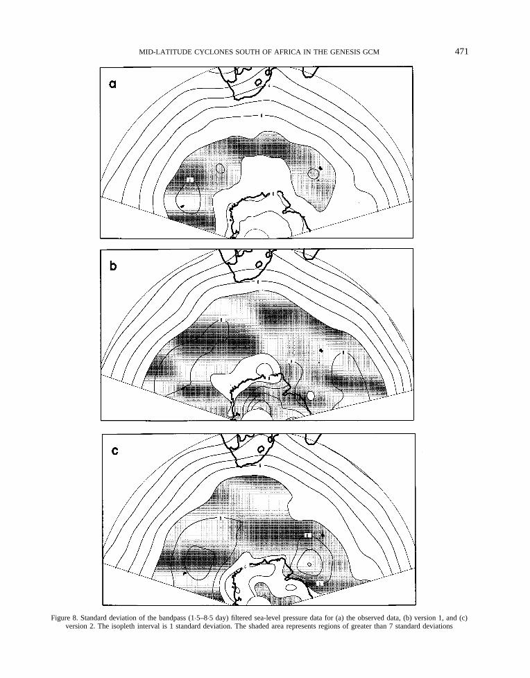
Figure 8. Standard deviation of the bandpass (1�5–8�5 day) filtered sea-level pressure data for (a) the observed data, (b) version 1, and (c)version 2. The isopleth interval is 1 standard deviation. The shaded area represents regions of greater than 7 standard deviations


which is thought to be due to insufficient resolution to deal with dynamics related to the steep Antarctictopography.

Version 1 of the GCM exhibits anomalously high cyclone densities north of about 55�S and the band of highcyclone densities around the Antarctic continent is not well defined. The high densities north of 55�S could belinked to the overly active convective plume scheme in version 1 and/or the anomalously high horizontal heattransport to higher latitudes, which may lead to enhanced energy input into the atmosphere and potentially morecyclogenesis. The convective plume scheme has been improved in version 2 and horizontal heat transport is morerealistic. The under representation of cyclone densities in the region of the circumpolar trough in version 1, maybe related to the coarse resolution of the AGCM being unable to resolve mesocyclones and smaller scale synopticcyclones.

Version 2 of GENESIS is an improvement over version 1 in terms of the pattern and magnitude of cyclonedensities. However, north of 61�S there are still more cyclones than observed, and between 0� and 50�E theregion of high cyclone occurrence near the Antarctic continent appears to have been shifted slightly northwards.The greater densities of cyclones north of 61�S could be due, in part, to the finer grid of the model compared withthe observed data, meaning that smaller synoptic cyclones and mesocyclones may be resolved by the model, butnot by the observed data. The northward shift of cyclones between 0� and 50�E in the high density circumpolarcore of version 2, may be related to mean sea-ice extent being slightly northward in the model compared withwhat is observed.

Plots of zonally averaged cyclone central pressures show that version 1 does not simulate the full range ofcentral pressures, whereas version 2 is closer to the observed profile. In terms of the standard deviation of thebandpass filtered sea-level pressure data, both versions of the model exhibit greater variability compared with theobserved data.

The comparisons have shown that version 2 of GENESIS performs significantly better than its predecessor atsimulating mid-latitude cyclones south of Africa and has produced results remarkably similar to those generatedfrom the observed data. This provides those researchers who are using GENESIS to examine the possible regionalimpacts of global climate change on precipitation in southern Africa, with greater confidence in the use of version2, especially in terms of the simulation of mid-latitude cyclones. These cyclones provide the south-western tip ofSouth Africa with winter rainfall. It is likely that many of the discrepancies between the model-generated data(version 2) and the observed data would be eliminated if the model were to operate on a yet finer resolution (e.g.T42), and also if observed data of a comparable grid resolution to the model were to be used for the validationprocess.

ACKNOWLEDGEMENTS

The authors would like to thank the Earth Systems Science Centre at Pennsylvania State University,Pennsylvania, and the National Centre for Atmospheric Research, Boulder, Colorado, for allowing access to theGENESIS model. Financial support provided to D. Hudson by the Foundation for Research Development, SouthAfrica, over the period of this research is much appreciated. Thanks are also due to the two anonymous reviewersfor their very helpful comments.

REFERENCES

Barron, E. J., Peterson, W. W., Pollard, D. and Thompson, S. L. 1993. ‘Past climate and the role of ocean heat transport: model simulations forthe Cretaceous’,Paleoceanography,8, 785–798.

Barron, E. J., Fawcett, P. J., Peterson, W. W., Pollard, D. and Thompson, S. L. 1995. ‘A "simulation" of mid-Cretaceous climate’,Paleoceanography, 10, 853–962.

Bromwich, D. H., Chen, B. and Pan, X. 1995. ‘Intercomparison of simulated polar climates by global climate models’,Sixth Symposium onGlobal Climate Change, American Meteorological Society, Dallas, Texas, 15–20 January 1995, Pre-prints Volume (J9), pp. 14–19.

Carleton, A. M. 1979. ‘A synoptic climatology of satellite-observed extratropical cyclone activity for the southern hemisphere winter’,Arch.Meteorol. Geophys. Bioklimatol. Ser B.,27, 265–279.

Carleton, A. M. 1995. ‘On the interpretation and classification of mesoscale cyclones from satellite infrared imagery’,Int. J. Remote Sensing,16,(13), 2457–2485.

Carleton, A. M. and Carpenter, D. A. 1990. ‘Satellite climatology of ‘Polar Lows’ and broadscale climatic associations for the southernhemisphere’,Int. J. Climatol, 10, 219–246.


Cess, R. D., Zhang, M. H., Minnis, P., Corsetti, L., Dutton, E. G., Forgan, B. W., Garber, D. P., Gates, W. L., Hack, J. J., Harrison, E. F., Jing,X., Kiehl, J. T., Long, C. N., Morcrette, J. -J., Potter, G. L., Ramanathan, V., Subasilar, B., Whitlock, C. H., Young, D. F. and Zhou, Y.1995. ‘Absorption of solar radiation by clouds: observations versus models’,Science, 267, 496–499.

Changnon, D., Noel, J. J. and Maze, L. H. 1995. ‘Determining cyclone frequencies using equal-area circles’,Mon. Wea. Rev.,123, 2285–2294.Cogley, J. G. 1991.GGHYDRO—Global Hydrographic Data Release 2.0, Trent Climate Note 91-1, Trent University, Peterborough, Ontario,

Canada.Crowley, T. J. and Baum, S. K. 1994. ‘General circulation model study of late Carboniferous interglacial climates’,Palaeoclimates, 1, 3–21.Crowley, T. J., Baum, S. K. and Kim, K. Y. 1993. ‘General circulation model experiments with pole-centred supercontinents’,J. Geophys.

Res., 98, 8793–8800.Crowley, T. J., Yip, K. J., Baum, S. K. and Moore, S. B. 1996. ‘Modelling Carboniferous coal formation’,Paleoclimates, 2, 159–177.Cuming, M. J. and Hawkins, B. A. 1981.TERDAT: The FNOC System for Terrain Data Extraction and Processing’, Technical Report M11

project M254 (2nd ed), prepared for Fleet Numerical Oceanography Centre, Monterey, California. Published by Meteorology InternationalIncorporated.

Foley, J. A. 1994. ‘The sensitivity of the terrestrial biosphere to climatic change: a simulation of the middle Holocene’,Glob. Biogeochem.Cycles, 8, 505–525.

Jenkins, G. 1995. ‘Early earth’s climate: cloud feedback from reduced land fractions and ozone concentrations’,Geophys. Res. Lett., 22,1513–1516.

Jones, D. A. and Simmonds, I. 1993. ‘A climatology of southern hemisphere extratropical cyclones’,Climate Dyn., 9, 131–145.Kep, S. L. 1984.A Climatology of Cyclogenesis, Cyclone Tracks and Cyclolysis in the Southern Hemisphere for the Period 1972–81,

University of Melbourne, Department of Meteorology, publication 25.Kineman, J. (ed.) 1985.FNOC/NCAR Global Elevation, Terrain, and Surface Characteristics, Digital Dataset, 28 MB. NOAA National

Geophysical Data Centre, Boulder, Colorado.Konig, W., Sausen, R. and Sielmann, F. 1993. ‘Objective identification of cyclones in GCM simulations’,J. Climate,6, 2217–2231.Lambert, S. J. 1988. ‘A cyclone climatology of the Canadian Climate Centre general circulation model’,J. Climate, 1, 109–115.Le Marshall, J. F. and Kelly, G. A. M. 1981. ‘A January and July climatology of the Southern Hemisphere based on daily numerical analyses

1973–77’,Aust. Meteorol. Mag.,29, 115–123.Le Marshall, J. F., Kelly, G. A. M. and Karoly, D. J. 1985. ‘An atmospheric climatology of the Southern Hemisphere based on ten years of

daily numerical analyses (1972–82): I. overview’,Aust. Meteorol. Mag.,33, 65–85.Le Treut, H. and Kalnay, E. 1990. ‘Comparison of observed and simulated cyclone frequency distribution as determined by an objective

method’,Atmosphera., 3, 57–71.Murray, R. J. and Simmonds, I. 1991a. ‘A numerical scheme for tracking cyclone centres from digital data. Part 1: development of the

scheme’,Aust. Meteorol. Mag.,39, 155–166.Murray, R. J. and Simmonds, I. 1991b. ‘A numerical scheme for tracking cyclone centres from digital data. Part 2: application to January and

July general circulation model simulations’,Aust. Meteorol. Mag.,39, 167–180.Otto-Bliesner, B. L. 1993. ‘Tropical mountains and coal formation: a climate model study of the Westphalian (306 Ma)’,Geophys. Res. Lett.

20, 1947–1950.Ramanathan, V., Subasilar, B., Zhang, G. J., Conant, W., Cess, R. D., Kiehl, J. T., Grassl, H. and Shi, L. 1995. ‘Warm pool heat budget and

shortwave cloud forcing: a missing physics?’,Science, 267, 499–503.Senior, C. A. and Mitchell, J. F. B. 1993. ‘Carbon dioxide and climate: the impact of cloud parameterization’,J. Climate,6, 393–418.Serreze, M. C., Box, J. E., Barry, R. G. and Walsh, J. E. 1993. ‘Characteristics of Arctic synoptic activity, 1952–1989’,Meteorol. Atmos.

Phys., 51, 147–164.Sinclair, M. R. 1994. ‘An objective cyclone climatology for the southern hemisphere’,Mon. Wea. Rev.,122, 2239–2256.Sinclair, M. R. 1995. ‘A climatology of cyclogenesis for the southern hemisphere’,Mon. Wea. Rev.,123, 1601–1619.Slingo, A. and Slingo, J. M. 1991. ‘Response of the National Centre for Atmospheric Research community climate model to improvements in

the representation of clouds’,J. Geophys. Res.,96, 15341–15357.Smith, R. N. B. 1990. ‘A scheme for predicting layer clouds and their water content in a general circulation model’,Q. J. R. Meteorol. Soc.,

116, 435–460.Streten, N. A. and Troup, A. J. 1973. ‘A synoptic climatology of satellite observed cloud vortices over the southern hemisphere’,Q. J. R.

Meteorol. Soc.,99, 56–72.Swanson, G. S. and Trenberth, K. E. 1981. ‘Interannual variability in the Southern Hemisphere troposphere’,Mon. Wea. Rev.,109, 1890–

1897.Taljaard, J. J. 1967. ‘Development, distribution, and movement of cyclones and anticyclones in the southern hemisphere during the IGY’,J.

Appl. Meteorol.,6, 973–987.Thompson, S. L. and Pollard, D. 1995. ‘A global climate model (GENESIS) with a land-surface-transfer scheme (LSX). Part 1: present-day

climate’, J. Climate, 8, 732–761.Thompson, S. L. and Pollard, D. 1997. ‘Greenland and Antarctic mass balances for present and doubled CO2 from the GENESIS version 2

global climate model’,J. Climate, in press.Thompson, S. L., Ramaswamy, V. and Covey, C. 1987. ‘Atmospheric effects of nuclear war aerosols in general circulation model simulations:

influence of smoke optical properties’,J. Geophys. Res.,92, 10942–10960.Trenberth, K. E. 1979. ‘Interannual variability of the 500 mb zonal mean flow in the Southern Hemisphere’,Mon. Wea. Rev.,107, 1515–1524.Trenberth, K. E. 1991. ‘Storm tracks in the Southern Hemisphere’,J. Atmos. Sci.,48, 2159–2178.Van Bebber, W. J. 1882. ‘Typische Witterungsercheimungen’,Archiv Dt. Seewarte Hamburg,5(3), 45.Van Loon, H. 1965. ‘A climatological study of the atmospheric circulation in the Southern Hemisphere during the IGY, Part 1: 1 July 1957–31

March 1958’,J. Appl. Meteorol.4, 479–491.Wallace, J. M., Lim, G. -H. and Blackmon, M. L. 1988. ‘Relationship between cyclone tracks, anticyclone tracks, and baroclinic waveguides’,

J. Atmos. Sci.,45, 439–462.Willmott, C. J., Clinton, M. R. and Philpot, W. D. 1985. ‘Small-scale climate maps: a sensitivity analysis of some common assumptions

associated with grid-point interpolation and contouring’,Am. Cartogr., 12(1), 5–161.


mid-latitude cyclones south of africa in the genesis gcm

Documents