mid-pliocene climate modelled using the uk hadley centre

Geosci. Model Dev., 5, 1109–1125, 2012www.geosci-model-dev.net/5/1109/2012/doi:10.5194/gmd-5-1109-2012© Author(s) 2012. CC Attribution 3.0 License.

GeoscientificModel Development

Mid-Pliocene climate modelled using the UK Hadley Centre Model:PlioMIP Experiments 1 and 2

F. J. Bragg1, D. J. Lunt1, and A. M. Haywood2

1BRIDGE, School of Geographical Sciences, University of Bristol, University Road, Bristol, BS8 1SS, UK2School of Earth and Environment, University of Leeds, Woodhouse Lane, Leeds, LS2 9JT, UK

Correspondence to:F. J. Bragg ([email protected])

Received: 13 March 2012 – Published in Geosci. Model Dev. Discuss.: 18 April 2012Revised: 7 August 2012 – Accepted: 8 August 2012 – Published: 13 September 2012

Abstract. The Pliocene Model Intercomparison Project(PlioMIP) is a sub-project of the Paleoclimate Modelling In-tercomparison Project (PMIP) whose objective is to comparepredictions of the mid-Pliocene climate from the widest pos-sible range of general circulation models. The mid-Pliocene(3.3–3.0 Ma) is the most recent sustained period of greaterwarmth and atmospheric carbon dioxide concentration thanthe pre-industrial times and as such has potential to in-form predictions of our warming climate in the coming cen-tury. This paper describes the UK contribution to PlioMIPusing the Hadley Centre Model both in atmosphere-onlymode (HadAM3, PlioMIP Experiment 1) and atmosphere-ocean coupled mode (HadCM3, PlioMIP Experiment 2). Thecoupled model predicts a greater overall warming (3.3◦C)relative to the control than the atmosphere-only (2.5◦C).The Northern Hemisphere latitudinal temperature gradientis greater in the coupled model with a warmer Equator andcolder Arctic than the atmosphere-only model, which is con-strained by sea surface temperatures from Pliocene proxy re-constructions. The atmosphere-only model predicts a reduc-tion in equatorial precipitation and south Asian monsoon in-tensity, whereas the coupled model shows an increase in theintensity of these systems. We present sensitivity studies us-ing alternative boundary conditions for both the Pliocene andthe control simulations, indicating the sensitivity of the mid-Pliocene warming to uncertainties in both pre-industrial andmid-Pliocene climate.

1 Introduction

This paper describes the Pliocene Model IntercomparisonProject (PlioMIP) simulations carried out using the UK Me-teorological Office Hadley Centre Model (HadAM3 andHadCM3).

General circulation models (GCMs) are one of the maintools used for studying the climate system of the present dayand the past and to predict likely climate changes that canbe expected in the future. These models vary significantly inthe way they parameterise certain complex processes and assuch vary in their simulation of the modern climate as well asin their past and future predictions. The Paleoclimate Mod-elling Project (PMIP, seehttp://pmip3.lsce.ipsl.fr/) exists tocreate intercomparisons of the widest possible range of mod-els forced as nearly as possible with identical palaeo bound-ary conditions. The intercomparisons focus on different timeslices of particular interest to the scientific community, in-cluding the Last Glacial Maximum (21 kyr), Last Interglacial(130 kyr, 125 kyr and 115 kyr) and Mid-Holocene (6 kyr) andmore recently extended to 8.2 kyr and Pliocene, specificallythe mid-Pliocene warm period (MPWP) from 3.29–2.97 Ma(Haywood et al., 2010).

The Pliocene is of particular interest for the develop-ment of the GCMs used in future climate predictions asit is the most recent sustained period that is significantlywarmer than the present day and thus the climate systemmay operate in a similar manner to potential climates of thecoming century. A substantial dataset describing the MPWPtime slab has been assembled by the US Geological SurveyPRISM project (Pliocene Research, Interpretation and Syn-optic Mapping,http://geology.er.usgs.gov/eespteam/prism/),

Published by Copernicus Publications on behalf of the European Geosciences Union.

http://pmip3.lsce.ipsl.fr/

http://geology.er.usgs.gov/eespteam/prism/

1110 F. J. Bragg et al.: Mid-Pliocene climate modelled using the UK Hadley Centre Model

Control

Expts 1 & 2

Pliocene

Expt 1

Pliocene

Expt 2

a) c) b)

f) e) d)

Fig. 1. Summary of land surface boundary conditions for PlioMIP simulations: panels(a)–(c) show orography projected onto the appro-priate land-sea mask for control, Experiment 1 and Experiment 2 Pliocene simulations. Panels(d)–(f) show snow-free albedo for control,Experiment 1 and Experiment 2 Pliocene simulations – values above 0.3 shown in beige represent ice sheets.

including topography data, sea surface temperatures, vege-tation reconstruction and ice sheet extents and topography(Dowsett et al., 2010). These data are used to force the mod-els to achieve consistent simulations of how the Pliocene cli-mate differs from the pre-industrial control.

This paper describes the implementation of the PRISM3boundary conditions for use with the UK Hadley CentreModel according to the PlioMIP protocols for atmosphere-only models: “Experiment 1” (Haywood et al., 2010), andcoupled ocean-atmosphere models: “Experiment 2” (Hay-wood et al., 2011). We also provide a summary of the basicresults and some initial analysis including model-data com-parison.

2 Model description

We use the UK Meteorological Office Hadley Centre Model,also known as the Unified Model (UM) for these experi-ments, specifically the atmosphere-only version, HadAM3(Pope et al., 2000), for Experiment 1 and the coupled ocean-atmosphere version, HadCM3 (Gordon et al., 2000), for Ex-periment 2.

2.1 Atmosphere

The atmosphere module has a resolution of 96× 73 gridpoints (3.75◦ × 2.5◦) and 19 vertical levels using a hybridσ -pressure grid with a timestep of 0.5 h. An Arakawa B-grid(Arakawa and Lamb, 1977) is used in the horizontal planeto improve accuracy, with thermodynamic variables stored atthe centre of the grid and wind components at the corners(Johns et al., 1997).

The atmosphere-only model specifies 12 mid-monthlyfields of sea surface temperature as boundary conditions,which are interpolated to daily values at run-time.

A convection scheme developed by Gregory et al. (1997)is included which accounts for the direct effects of convec-tion on momentum. A first order scheme for turbulent ver-tical mixing of momentum and thermodynamic quantities isused within the boundary layer, which can occupy up to thefirst 5 layers of the model (Smith, 1990). Sub grid-scale grav-ity wave and orographic drag parameterisations include theimpact of orographic variance anisotropy (Milton and Wil-son, 1996; Gregory et al., 1998).

Clouds are modelled as either water, ice or mixed-phasebetween 0 and−9 ◦C. Clouds are aggregated into 3 layers

Geosci. Model Dev., 5, 1109–1125, 2012 www.geosci-model-dev.net/5/1109/2012/

F. J. Bragg et al.: Mid-Pliocene climate modelled using the UK Hadley Centre Model 1111

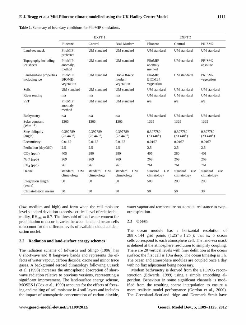
Table 1.Summary of boundary conditions for PlioMIP simulations.

EXPT 1 EXPT 2

Pliocene Control BAS Modern Pliocene Control PRISM2

Land-sea mask PlioMIPpreferred

UM standard UM standard UM standard UM standard UM standard

Topography includingice sheets

PlioMIPanomalymethod

UM standard UM standard PlioMIPanomalymethod

UM standard PRISM2absolute

Land-surface propertiesincluding ice

PlioMIPBIOME4vegetation

UM standard BAS-Observmodernvegetation

PlioMIPBIOME4vegetation

UM standard PRISM2vegetation

Soils UM standard UM standard UM standard UM standard UM standard UM standard

River routing n/a n/a n/a UM standard UM standard UM standard

SST PlioMIPanomalymethod

UM standard UM standard n/a n/a n/a

Bathymetry n/a n/a n/a UM standard UM standard UM standard

Solar constant(W m−2)

1365 1365 1365 1365 1365 1365

Sine obliquity(angle)

0.397789(23.440◦)

0.397789(23.440◦)

0.397789(23.440◦)

0.397789(23.440◦)

0.397789(23.440◦)

0.397789(23.440◦)

Eccentricity 0.0167 0.0167 0.0167 0.0167 0.0167 0.0167

Perihelion (day/360) 2.5 2.5 2.5 2.5 2.5 2.5

CO2 (ppm) 405 280 280 405 280 401

N2O (ppb) 269 269 269 269 269 269

CH4 (ppb) 761 761 761 761 761 761

Ozone standard UMclimatology

standard UMclimatology





Integration length(years)

50 50 50 500 200 200

Climatological means 30 30 30 50 50 30

(low, medium and high) and form when the cell moisturelevel standard deviation exceeds a critical level of relative hu-midity, RHcrit = 0.7. The threshold of total water content forprecipitation to occur is varied between land and ocean cellsto account for the different levels of available cloud conden-sation nuclei.

2.2 Radiation and land-surface energy schemes

The radiation scheme of Edwards and Slingo (1996) has6 shortwave and 8 longwave bands and represents the ef-fects of water vapour, carbon dioxide, ozone and minor tracegases. A background aerosol climatology following Cusacket al. (1998) increases the atmospheric absorption of short-wave radiation relative to previous versions, representing asignificant improvement. The land-surface energy scheme,MOSES I (Cox et al., 1999) accounts for the effects of freez-ing and melting of soil moisture in 4 soil layers and includesthe impact of atmospheric concentration of carbon dioxide,

water vapour and temperature on stomatal resistance to evap-otranspiration.

2.3 Ocean

The ocean module has a horizontal resolution of288× 144 grid points (1.25◦ × 1.25◦): that is, 6 oceancells correspond to each atmosphere cell. The land-sea maskis defined at the atmosphere resolution to simplify coupling.There are 20 vertical levels with finer definition at the oceansurface: the first cell is 10m deep. The ocean timestep is 1 h.The ocean and atmosphere modules are coupled once a daywith no flux adjustment being necessary.

Modern bathymetry is derived from the ETOPO5 recon-struction (Edwards, 1989) using a simple smoothing al-gorithm. Behaviour in some significant channels is mod-ified from the resulting coarse interpolation to ensure amore realistic model performance (Gordon et al., 2000).The Greenland–Scotland ridge and Denmark Strait have

www.geosci-model-dev.net/5/1109/2012/ Geosci. Model Dev., 5, 1109–1125, 2012


Control

Expt 1

Pliocene

Expt 1

a) b)

d) c)

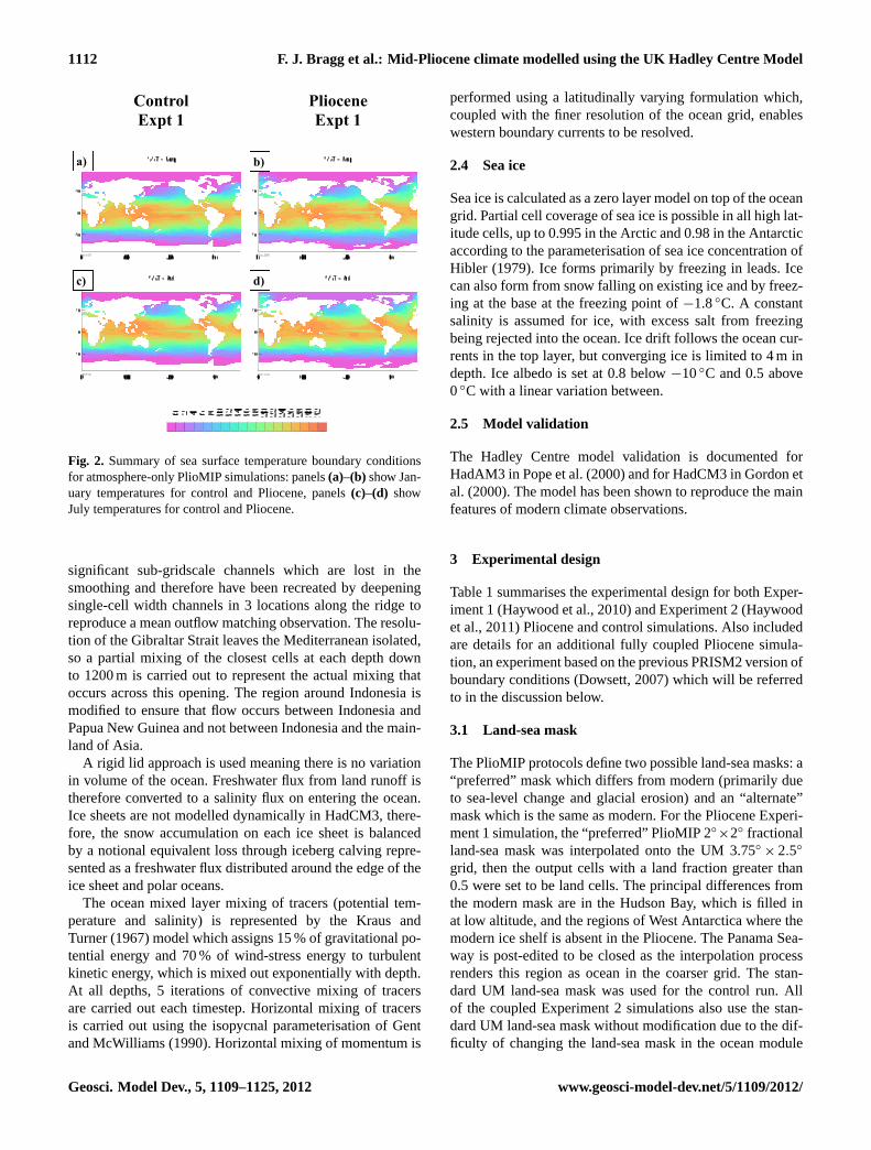
Fig. 2. Summary of sea surface temperature boundary conditionsfor atmosphere-only PlioMIP simulations: panels(a)–(b) show Jan-uary temperatures for control and Pliocene, panels(c)–(d) showJuly temperatures for control and Pliocene.

significant sub-gridscale channels which are lost in thesmoothing and therefore have been recreated by deepeningsingle-cell width channels in 3 locations along the ridge toreproduce a mean outflow matching observation. The resolu-tion of the Gibraltar Strait leaves the Mediterranean isolated,so a partial mixing of the closest cells at each depth downto 1200 m is carried out to represent the actual mixing thatoccurs across this opening. The region around Indonesia ismodified to ensure that flow occurs between Indonesia andPapua New Guinea and not between Indonesia and the main-land of Asia.

A rigid lid approach is used meaning there is no variationin volume of the ocean. Freshwater flux from land runoff istherefore converted to a salinity flux on entering the ocean.Ice sheets are not modelled dynamically in HadCM3, there-fore, the snow accumulation on each ice sheet is balancedby a notional equivalent loss through iceberg calving repre-sented as a freshwater flux distributed around the edge of theice sheet and polar oceans.

The ocean mixed layer mixing of tracers (potential tem-perature and salinity) is represented by the Kraus andTurner (1967) model which assigns 15 % of gravitational po-tential energy and 70 % of wind-stress energy to turbulentkinetic energy, which is mixed out exponentially with depth.At all depths, 5 iterations of convective mixing of tracersare carried out each timestep. Horizontal mixing of tracersis carried out using the isopycnal parameterisation of Gentand McWilliams (1990). Horizontal mixing of momentum is

performed using a latitudinally varying formulation which,coupled with the finer resolution of the ocean grid, enableswestern boundary currents to be resolved.

2.4 Sea ice

Sea ice is calculated as a zero layer model on top of the oceangrid. Partial cell coverage of sea ice is possible in all high lat-itude cells, up to 0.995 in the Arctic and 0.98 in the Antarcticaccording to the parameterisation of sea ice concentration ofHibler (1979). Ice forms primarily by freezing in leads. Icecan also form from snow falling on existing ice and by freez-ing at the base at the freezing point of−1.8◦C. A constantsalinity is assumed for ice, with excess salt from freezingbeing rejected into the ocean. Ice drift follows the ocean cur-rents in the top layer, but converging ice is limited to 4 m indepth. Ice albedo is set at 0.8 below−10◦C and 0.5 above0◦C with a linear variation between.

2.5 Model validation

The Hadley Centre model validation is documented forHadAM3 in Pope et al. (2000) and for HadCM3 in Gordon etal. (2000). The model has been shown to reproduce the mainfeatures of modern climate observations.

3 Experimental design

Table 1 summarises the experimental design for both Exper-iment 1 (Haywood et al., 2010) and Experiment 2 (Haywoodet al., 2011) Pliocene and control simulations. Also includedare details for an additional fully coupled Pliocene simula-tion, an experiment based on the previous PRISM2 version ofboundary conditions (Dowsett, 2007) which will be referredto in the discussion below.

3.1 Land-sea mask

The PlioMIP protocols define two possible land-sea masks: a“preferred” mask which differs from modern (primarily dueto sea-level change and glacial erosion) and an “alternate”mask which is the same as modern. For the Pliocene Experi-ment 1 simulation, the “preferred” PlioMIP 2◦

×2◦ fractionalland-sea mask was interpolated onto the UM 3.75◦

× 2.5◦

grid, then the output cells with a land fraction greater than0.5 were set to be land cells. The principal differences fromthe modern mask are in the Hudson Bay, which is filled inat low altitude, and the regions of West Antarctica where themodern ice shelf is absent in the Pliocene. The Panama Sea-way is post-edited to be closed as the interpolation processrenders this region as ocean in the coarser grid. The stan-dard UM land-sea mask was used for the control run. Allof the coupled Experiment 2 simulations also use the stan-dard UM land-sea mask without modification due to the dif-ficulty of changing the land-sea mask in the ocean module



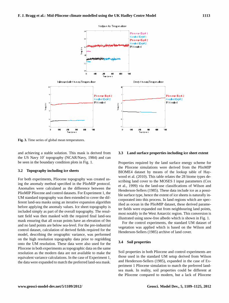
Fig. 3.Time series of global mean temperatures.

and achieving a stable solution. This mask is derived fromthe US Navy 10′ topography (NCAR/Navy, 1984) and canbe seen in the boundary condition plots in Fig. 1.

3.2 Topography including ice sheets

For both experiments, Pliocene topography was created us-ing the anomaly method specified in the PlioMIP protocol.Anomalies were calculated as the difference between thePlioMIP Pliocene and control datasets. For Experiment 1, theUM standard topography was then extended to cover the dif-ferent land-sea masks using an iterative expansion algorithmbefore applying the anomaly values. Ice sheet topography isincluded simply as part of the overall topography. The resul-tant field was then masked with the required final land-seamask ensuring that all ocean points have an elevation of 0mand no land points are below sea-level. For the pre-industrialcontrol dataset, calculation of derived fields required for themodel, describing the orographic variance, was performedon the high resolution topography data prior to regriddingonto the UM resolution. These data were also used for thePliocene in both experiments as topographic data on the sameresolution as the modern data are not available to make theequivalent variance calculations. In the case of Experiment 1,the data were expanded to match the preferred land-sea mask.

3.3 Land surface properties including ice sheet extent

Properties required by the land surface energy scheme forthe Pliocene simulations were derived from the PlioMIPBIOME4 dataset by means of the lookup table of Hay-wood et al. (2010). This table relates the 28 biome types de-scribing land cover to the MOSES I input parameters (Coxet al., 1999) via the land-use classifications of Wilson andHenderson-Sellers (1985). These data include ice as a possi-ble surface type, hence the extent of ice sheets is naturally in-corporated into this process. In land regions which are spec-ified as ocean in the PlioMIP dataset, these derived parame-ter fields were expanded out from neighbouring land points,most notably in the West Antarctic region. This conversion isillustrated using snow-free albedo which is shown in Fig. 1.

For the control experiments, the standard UM dataset ofvegetation was applied which is based on the Wilson andHenderson-Sellers (1985) archive of land cover.

3.4 Soil properties

Soil properties in both Pliocene and control experiments arethose used in the standard UM setup derived from Wilsonand Henderson-Sellers (1985), expanded in the case of Ex-periment 1 Pliocene simulation to match the preferred land-sea mask. In reality, soil properties could be different atthe Pliocene compared to modern, but a lack of Pliocene



a) c) b)

f) e) d)

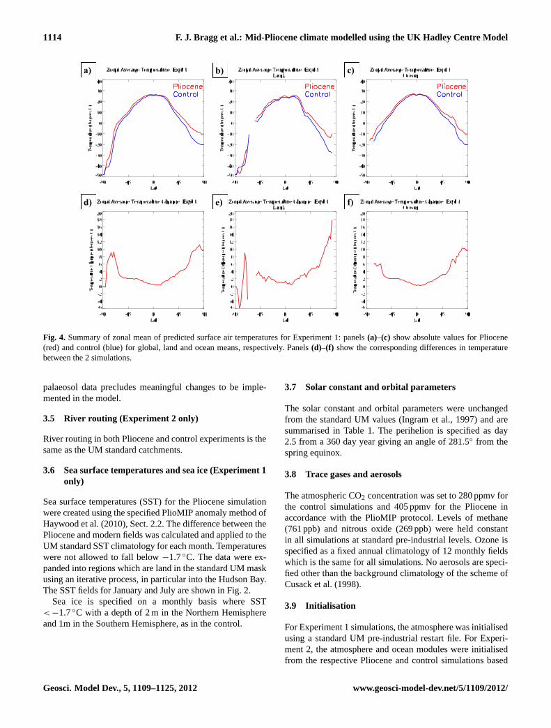
Fig. 4. Summary of zonal mean of predicted surface air temperatures for Experiment 1: panels(a)–(c) show absolute values for Pliocene(red) and control (blue) for global, land and ocean means, respectively. Panels(d)–(f) show the corresponding differences in temperaturebetween the 2 simulations.

palaeosol data precludes meaningful changes to be imple-mented in the model.

3.5 River routing (Experiment 2 only)

River routing in both Pliocene and control experiments is thesame as the UM standard catchments.

3.6 Sea surface temperatures and sea ice (Experiment 1only)

Sea surface temperatures (SST) for the Pliocene simulationwere created using the specified PlioMIP anomaly method ofHaywood et al. (2010), Sect. 2.2. The difference between thePliocene and modern fields was calculated and applied to theUM standard SST climatology for each month. Temperatureswere not allowed to fall below−1.7◦C. The data were ex-panded into regions which are land in the standard UM maskusing an iterative process, in particular into the Hudson Bay.The SST fields for January and July are shown in Fig. 2.

Sea ice is specified on a monthly basis where SST< −1.7◦C with a depth of 2 m in the Northern Hemisphereand 1m in the Southern Hemisphere, as in the control.

3.7 Solar constant and orbital parameters

The solar constant and orbital parameters were unchangedfrom the standard UM values (Ingram et al., 1997) and aresummarised in Table 1. The perihelion is specified as day2.5 from a 360 day year giving an angle of 281.5◦ from thespring equinox.

3.8 Trace gases and aerosols

The atmospheric CO2 concentration was set to 280 ppmv forthe control simulations and 405 ppmv for the Pliocene inaccordance with the PlioMIP protocol. Levels of methane(761 ppb) and nitrous oxide (269 ppb) were held constantin all simulations at standard pre-industrial levels. Ozone isspecified as a fixed annual climatology of 12 monthly fieldswhich is the same for all simulations. No aerosols are speci-fied other than the background climatology of the scheme ofCusack et al. (1998).

3.9 Initialisation

For Experiment 1 simulations, the atmosphere was initialisedusing a standard UM pre-industrial restart file. For Experi-ment 2, the atmosphere and ocean modules were initialisedfrom the respective Pliocene and control simulations based



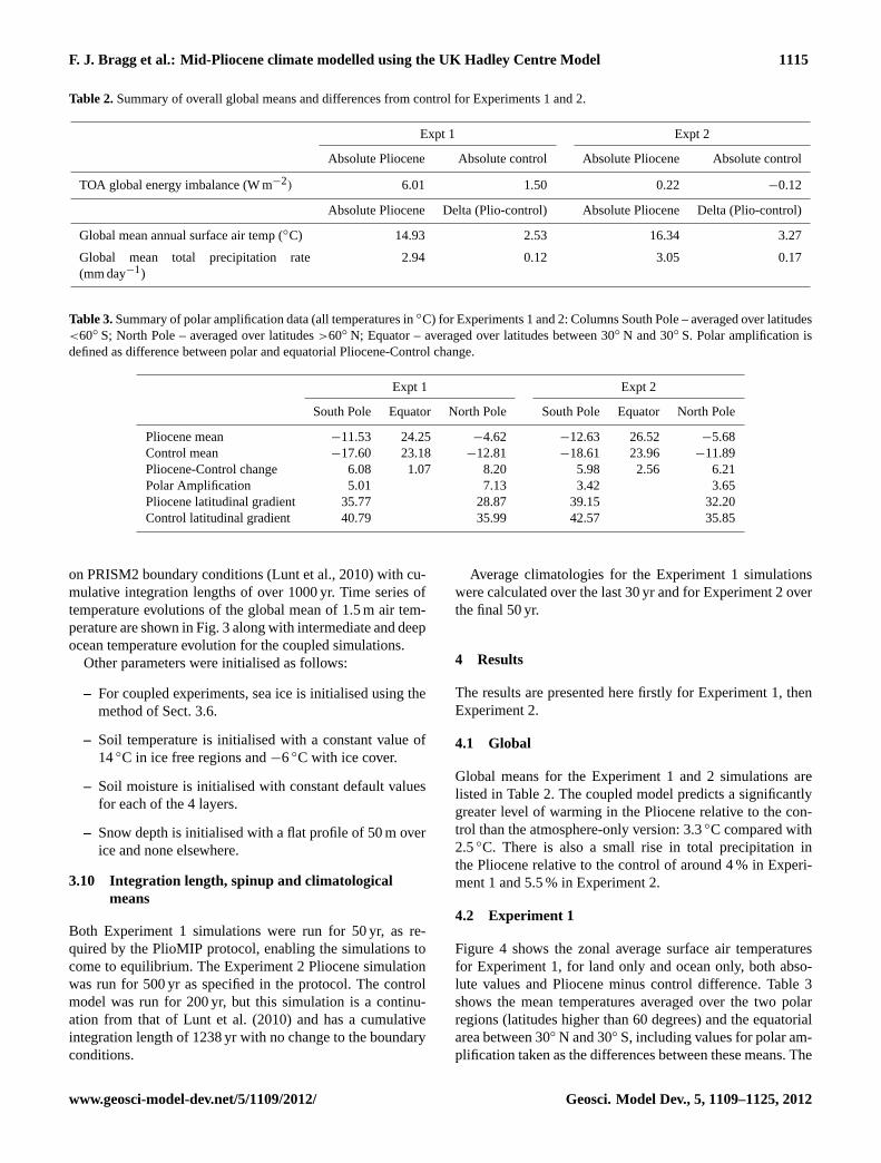
Table 2.Summary of overall global means and differences from control for Experiments 1 and 2.

Expt 1 Expt 2

Absolute Pliocene Absolute control Absolute Pliocene Absolute control

TOA global energy imbalance (W m−2) 6.01 1.50 0.22 −0.12

Absolute Pliocene Delta (Plio-control) Absolute Pliocene Delta (Plio-control)

Global mean annual surface air temp (◦C) 14.93 2.53 16.34 3.27

Global mean total precipitation rate(mm day−1)

2.94 0.12 3.05 0.17

Table 3.Summary of polar amplification data (all temperatures in◦C) for Experiments 1 and 2: Columns South Pole – averaged over latitudes<60◦ S; North Pole – averaged over latitudes>60◦ N; Equator – averaged over latitudes between 30◦ N and 30◦ S. Polar amplification isdefined as difference between polar and equatorial Pliocene-Control change.

Expt 1 Expt 2

South Pole Equator North Pole South Pole Equator North Pole

Pliocene mean −11.53 24.25 −4.62 −12.63 26.52 −5.68Control mean −17.60 23.18 −12.81 −18.61 23.96 −11.89Pliocene-Control change 6.08 1.07 8.20 5.98 2.56 6.21Polar Amplification 5.01 7.13 3.42 3.65Pliocene latitudinal gradient 35.77 28.87 39.15 32.20Control latitudinal gradient 40.79 35.99 42.57 35.85

on PRISM2 boundary conditions (Lunt et al., 2010) with cu-mulative integration lengths of over 1000 yr. Time series oftemperature evolutions of the global mean of 1.5 m air tem-perature are shown in Fig. 3 along with intermediate and deepocean temperature evolution for the coupled simulations.

Other parameters were initialised as follows:

– For coupled experiments, sea ice is initialised using themethod of Sect.3.6.

– Soil temperature is initialised with a constant value of14◦C in ice free regions and−6◦C with ice cover.

– Soil moisture is initialised with constant default valuesfor each of the 4 layers.

– Snow depth is initialised with a flat profile of 50 m overice and none elsewhere.

3.10 Integration length, spinup and climatologicalmeans

Both Experiment 1 simulations were run for 50 yr, as re-quired by the PlioMIP protocol, enabling the simulations tocome to equilibrium. The Experiment 2 Pliocene simulationwas run for 500 yr as specified in the protocol. The controlmodel was run for 200 yr, but this simulation is a continu-ation from that of Lunt et al. (2010) and has a cumulativeintegration length of 1238 yr with no change to the boundaryconditions.

Average climatologies for the Experiment 1 simulationswere calculated over the last 30 yr and for Experiment 2 overthe final 50 yr.

4 Results

The results are presented here firstly for Experiment 1, thenExperiment 2.

4.1 Global

Global means for the Experiment 1 and 2 simulations arelisted in Table 2. The coupled model predicts a significantlygreater level of warming in the Pliocene relative to the con-trol than the atmosphere-only version: 3.3◦C compared with2.5◦C. There is also a small rise in total precipitation inthe Pliocene relative to the control of around 4 % in Experi-ment 1 and 5.5 % in Experiment 2.

4.2 Experiment 1

Figure 4 shows the zonal average surface air temperaturesfor Experiment 1, for land only and ocean only, both abso-lute values and Pliocene minus control difference. Table 3shows the mean temperatures averaged over the two polarregions (latitudes higher than 60 degrees) and the equatorialarea between 30◦ N and 30◦ S, including values for polar am-plification taken as the differences between these means. The



Fig. 5. Summary of surface air temperatures for Experiment 1: panels(a)–(c) show annual mean temperatures for Pliocene and controlsimulations and the difference between them. Panels(d)–(f) similarly show the DJF means and panels(g)–(i) the JJA means.

difference profile (Fig. 4d) over the non-polar oceans fallsalmost to 0◦C around the Equator with a mean value acrossthe tropics of around 1◦C; this profile is strongly constrainedby the imposed sea surface temperature boundary condition.The latitudinal temperature gradient, especially in the North-ern Hemisphere is significantly reduced in the Pliocene rel-ative to the control (Fig. 4a–c). Polar amplification in thePliocene relative to the control is clear in the zonal profileswith mean values of around 5◦C in the Southern Hemisphereand 7◦C in the Northern Hemisphere.

These results are apparent in greater detail in Fig. 5 whichshows annual, DJF and JJA mean surface air temperature pat-terns for both Pliocene and control simulations and the dif-ference between them. The polar amplification is most pro-nounced in winter for both hemispheres. In the Antarctic, themajority of the warming maxima occur in regions which areocean in the Pliocene and land in the control simulation dueto the change in albedo and heat capacity, combined withsmaller areas on land where the ice sheet is at considerablylower altitude in the Pliocene model. Pliocene Arctic warm-ing is also associated with regions of change in the altitudeor extent of the Greenland icesheet in a similar manner to

the Antarctic. There is also a warming evident in the NorthAtlantic driven by the sea surface temperature boundary con-ditions which are significantly warmer than in the control.

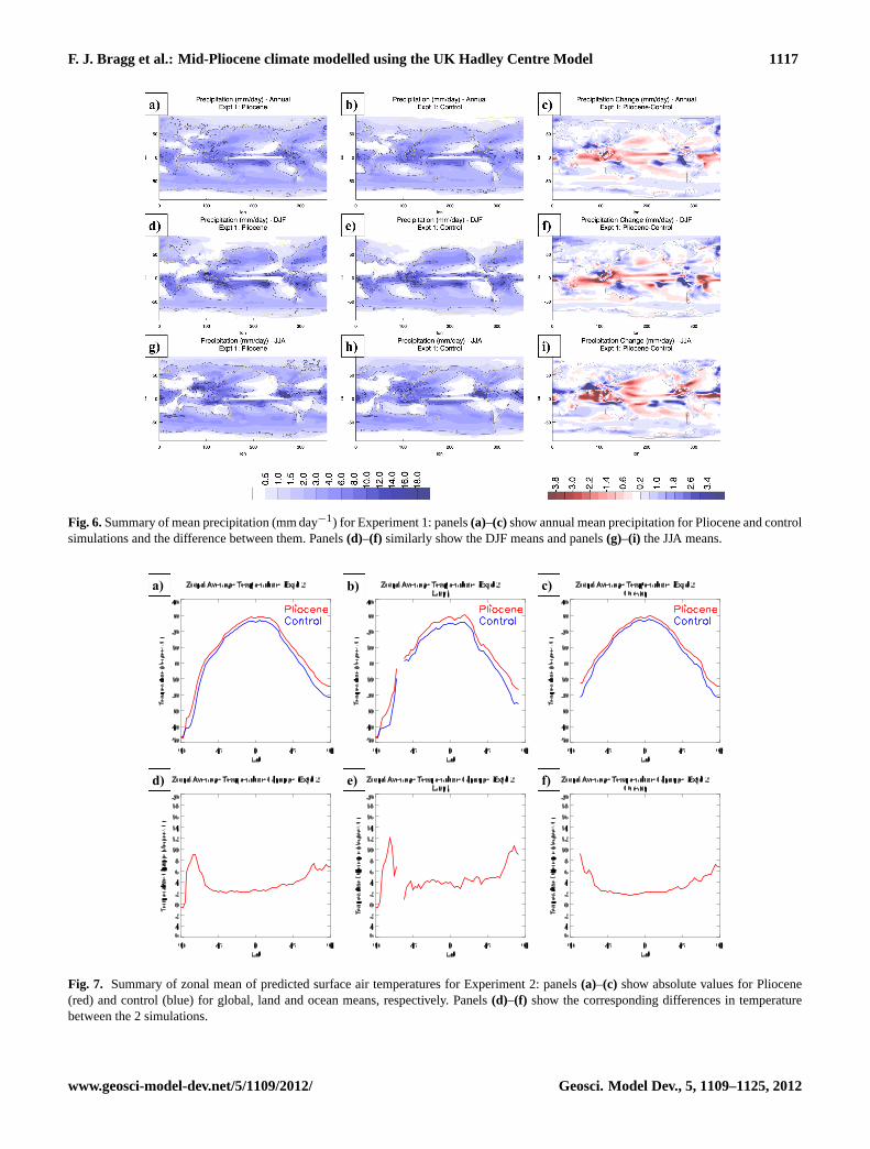
Figure 6 summarises the precipitation patterns for thePliocene and control experiments and the difference betweenthem, showing the annual, DJF and JJA means. There is areduction in equatorial rainfall in the Pliocene, especially inthe extent and intensity of the south Asian summer monsoonsystems.

4.3 Experiment 2

Figure 7 shows the zonal mean surface air temperatures glob-ally, for land only and ocean only along with Pliocene minuscontrol difference for Experiment 2. Mean polar and equa-torial temperatures and polar amplification values are listedin Table 3 as for Experiment 1 (Sect.4.2). Experiment 2shows more warming globally than Experiment 1 (3.3◦Ccompared with 2.5◦C, see Table 2) but this temperature in-crease is more evenly distributed latitudinally, with 2.5◦Cwarming in the equatorial zone and reduced polar amplifica-tion in both hemispheres of 3.5◦C. These results are shown



Fig. 6.Summary of mean precipitation (mm day−1) for Experiment 1: panels(a)–(c) show annual mean precipitation for Pliocene and controlsimulations and the difference between them. Panels(d)–(f) similarly show the DJF means and panels(g)–(i) the JJA means.

a) c) b)

f) e) d)

Fig. 7. Summary of zonal mean of predicted surface air temperatures for Experiment 2: panels(a)–(c) show absolute values for Pliocene(red) and control (blue) for global, land and ocean means, respectively. Panels(d)–(f) show the corresponding differences in temperaturebetween the 2 simulations.



Fig. 8. Summary of surface air temperatures for Experiment 2: panels(a)–(c) show annual mean temperatures for Pliocene and controlsimulations and the difference between them. Panels(d)–(f) similarly show the DJF means and panels(g)–(i) the JJA means.

as Experiment 2 minus Experiment 1 differences in Pliocene-control changes in Fig. 12. Figure 12a–c again highlights theincreased warming at lower latitudes and the reduction inpolar warming in Experiment 2, especially apparent in theNorthern Hemisphere. Taken together, the increased equato-rial warming and reduced polar warming of Experiment 2lead to an increased latitudinal temperature gradient, whichis broadly similar in shape to that predicted for the controlexperiment (see Fig. 7a), in contrast to the reduction in latitu-dinal gradient shown by the PRISM reconstruction, implicitin Fig. 4c. Outside of the polar latitudes, there is a distinctionbetween ocean and land warming in Experiment 2, typicallyclose to 2◦C over water and 4◦C on land (see Figs. 7e, f and8c).

This global shift in temperature is also apparent in greaterspatial detail in Fig. 8, which shows global temperature pat-terns for Experiment 2. Outside of the polar regions, there isvery little variation in temperature shift with latitude, onlythe marked difference between land and sea noted above.The difference in Experiment 1 and Experiment 2 patternsof temperature change are shown in Fig. 12d–f and confirmthe previous observations, i.e. the equatorial ocean warmsmore in Experiment 2, the poles warm less, especially in

winter and the land warms more than the oceans. The moststriking difference is in the far north Atlantic which showsgreatly reduced warming in Experiment 2 where the uncon-strained ocean in the coupled simulation is not reproducingthe “hotspot” in the PRISM3 sea surface temperature datawhich constrain Experiment 1.

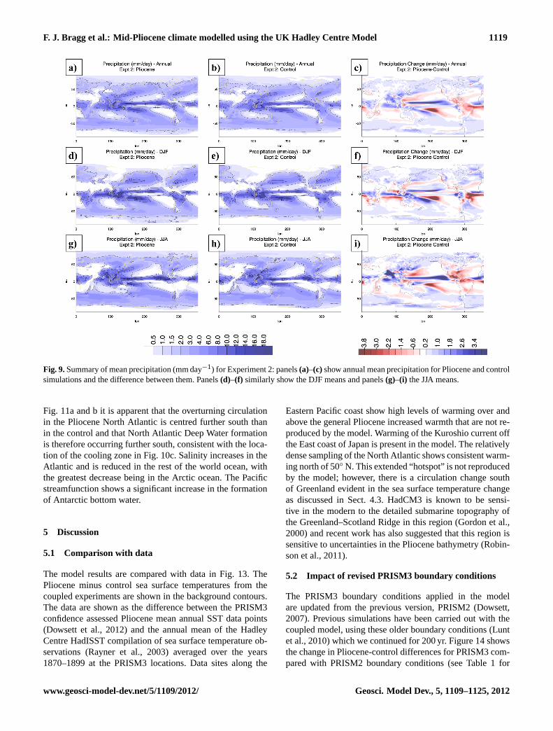
Figure 9 shows precipitation patterns for Experiment 2.The Pliocene minus control differences for Experiment 2are very different here from those seen for Experiment 1 inFig. 6. In this case, there is an increase in equatorial precip-itation and an intensification of the Indian monsoon. Thereis also a significant drying over equatorial South and CentralAmerica.

Figure 10 summarises the coupled model predicted seasurface temperatures and salinity for the Pliocene, controland the difference between them. Also shown are Atlantic(Fig. 11a and b) and Pacific (Fig. 11c and d) zonally av-eraged meridional overturning streamfunction. The changein sea surface temperature between the Pliocene and controlbroadly parallels that seen in surface air temperature over theoceans, a rise of the order of 2◦C in a fairly uniform dis-tribution. There is a distinct change in circulation south ofGreenland with adjacent warming and cooling zones. From



Fig. 9.Summary of mean precipitation (mm day−1) for Experiment 2: panels(a)–(c) show annual mean precipitation for Pliocene and controlsimulations and the difference between them. Panels(d)–(f) similarly show the DJF means and panels(g)–(i) the JJA means.

Fig. 11a and b it is apparent that the overturning circulationin the Pliocene North Atlantic is centred further south thanin the control and that North Atlantic Deep Water formationis therefore occurring further south, consistent with the loca-tion of the cooling zone in Fig. 10c. Salinity increases in theAtlantic and is reduced in the rest of the world ocean, withthe greatest decrease being in the Arctic ocean. The Pacificstreamfunction shows a significant increase in the formationof Antarctic bottom water.

5 Discussion

5.1 Comparison with data

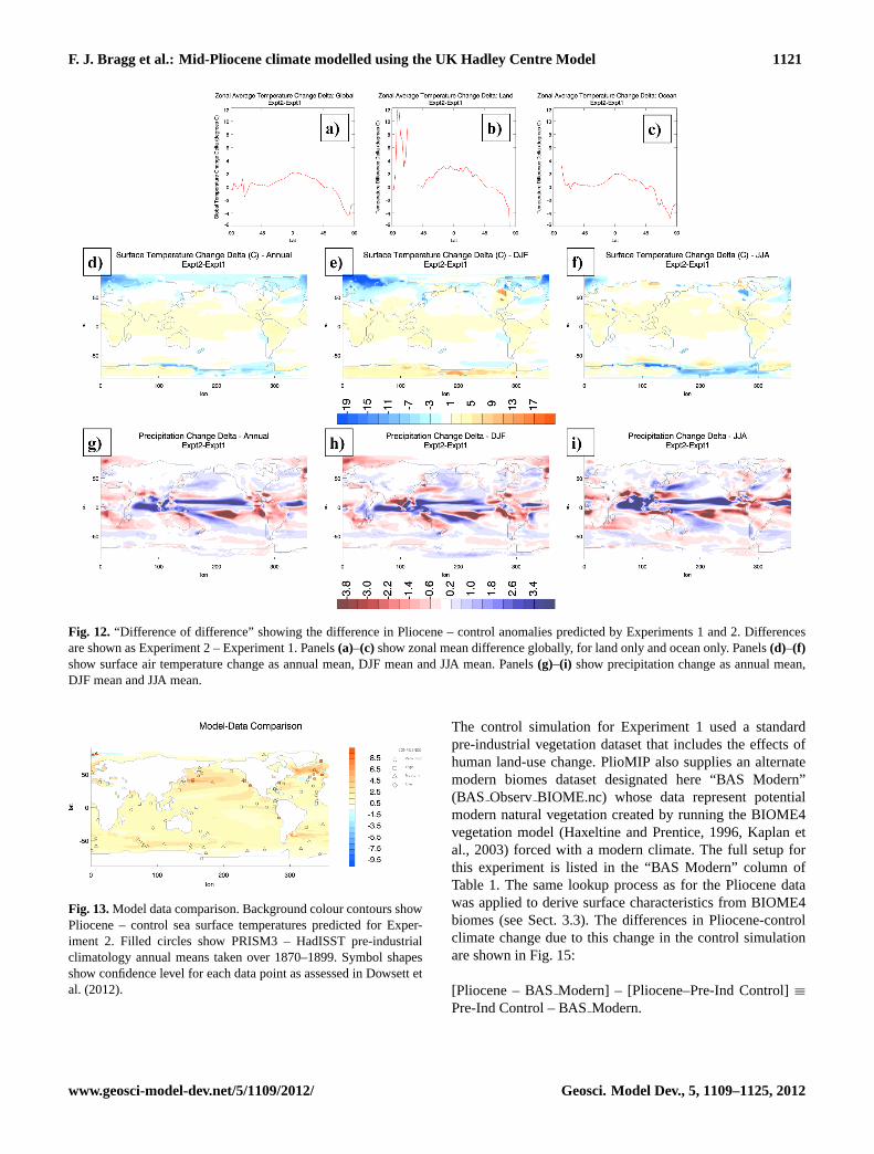
The model results are compared with data in Fig. 13. ThePliocene minus control sea surface temperatures from thecoupled experiments are shown in the background contours.The data are shown as the difference between the PRISM3confidence assessed Pliocene mean annual SST data points(Dowsett et al., 2012) and the annual mean of the HadleyCentre HadISST compilation of sea surface temperature ob-servations (Rayner et al., 2003) averaged over the years1870–1899 at the PRISM3 locations. Data sites along the

Eastern Pacific coast show high levels of warming over andabove the general Pliocene increased warmth that are not re-produced by the model. Warming of the Kuroshio current offthe East coast of Japan is present in the model. The relativelydense sampling of the North Atlantic shows consistent warm-ing north of 50◦ N. This extended “hotspot” is not reproducedby the model; however, there is a circulation change southof Greenland evident in the sea surface temperature changeas discussed in Sect.4.3. HadCM3 is known to be sensi-tive in the modern to the detailed submarine topography ofthe Greenland–Scotland Ridge in this region (Gordon et al.,2000) and recent work has also suggested that this region issensitive to uncertainties in the Pliocene bathymetry (Robin-son et al., 2011).

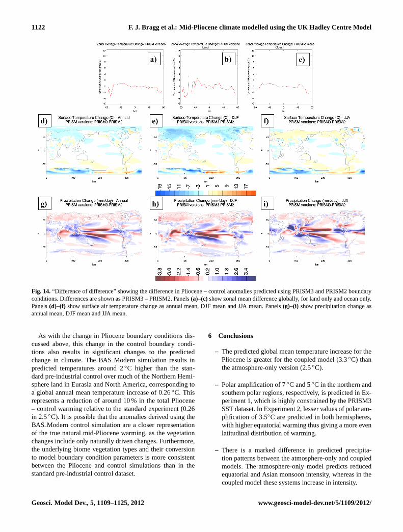
5.2 Impact of revised PRISM3 boundary conditions

The PRISM3 boundary conditions applied in the modelare updated from the previous version, PRISM2 (Dowsett,2007). Previous simulations have been carried out with thecoupled model, using these older boundary conditions (Luntet al., 2010) which we continued for 200 yr. Figure 14 showsthe change in Pliocene-control differences for PRISM3 com-pared with PRISM2 boundary conditions (see Table 1 for



Fig. 10.Summary of predicted ocean behaviour for Experiment 2: panels(a)–(c) show sea surface temperatures for Pliocene, control and thedifference between them; panels(d)–(f) similarly show salinity.

c)

a)

d)

b)

Fig. 11.Summary of predicted ocean behaviour for Experiment 2:Panels(a) and(b) show Atlantic overturning streamfunction for thePliocene and control and(c) and (d) show the Pacific overturningstreamfunction.

details of the PRISM2 model simulation). There is verylittle difference in the simulations in terms of PRISM3-PRISM2 global means: surface air temperature anomaly fallsby 0.05◦C and precipitation is unchanged to 3 significant fig-ures. At the regional level, however, there is a distinct in-crease in seasonality of temperature over much of the land inthe Northern Hemisphere. There are also temperature differ-ences where ice sheet topography has been updated and in re-gions of significant change to the orographic boundary condi-tions, notably the Rockies which show cooling with PRISM3topography even in summer when the rest of the NorthernHemisphere has a fairly uniform warming trend. Recent workhas interrogated the impact of each set of boundary condi-tions (CO2, orography, ice and vegetation) in the PRISM2simulations (Lunt et al., 2012), and a similar study is requiredfor the PRISM3 simulations in order to fully understand thechanges shown in Fig. 14, but this result serves to highlightthe significance of the uncertainty in boundary conditions onmodel predictions.

5.3 Impact of alternative vegetation data in controlexperiment

Here we examine the impact of using an alternate modernvegetation dataset in the Experiment 1 control simulation onthe prediction of Pliocene – pre-industrial climate change.



Fig. 12. “Difference of difference” showing the difference in Pliocene – control anomalies predicted by Experiments 1 and 2. Differencesare shown as Experiment 2 – Experiment 1. Panels(a)–(c) show zonal mean difference globally, for land only and ocean only. Panels(d)–(f)show surface air temperature change as annual mean, DJF mean and JJA mean. Panels(g)–(i) show precipitation change as annual mean,DJF mean and JJA mean.

Fig. 13.Model data comparison. Background colour contours showPliocene – control sea surface temperatures predicted for Exper-iment 2. Filled circles show PRISM3 – HadISST pre-industrialclimatology annual means taken over 1870–1899. Symbol shapesshow confidence level for each data point as assessed in Dowsett etal. (2012).

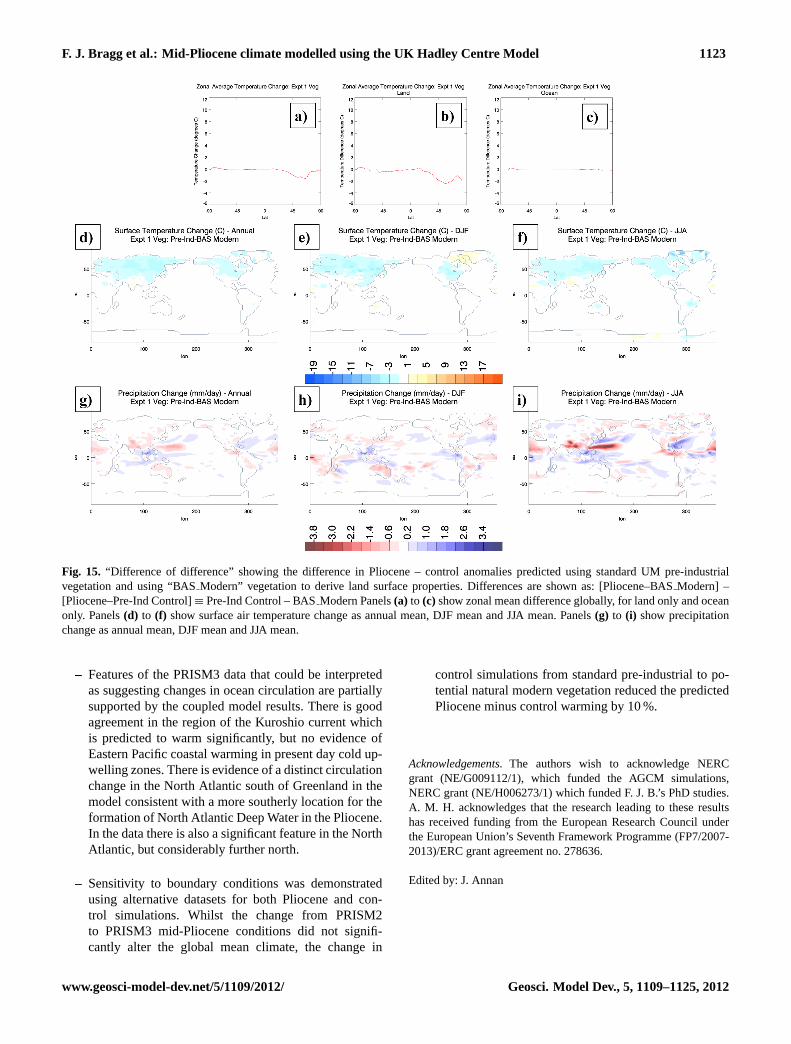
The control simulation for Experiment 1 used a standardpre-industrial vegetation dataset that includes the effects ofhuman land-use change. PlioMIP also supplies an alternatemodern biomes dataset designated here “BAS Modern”(BAS ObservBIOME.nc) whose data represent potentialmodern natural vegetation created by running the BIOME4vegetation model (Haxeltine and Prentice, 1996, Kaplan etal., 2003) forced with a modern climate. The full setup forthis experiment is listed in the “BAS Modern” column ofTable 1. The same lookup process as for the Pliocene datawas applied to derive surface characteristics from BIOME4biomes (see Sect.3.3). The differences in Pliocene-controlclimate change due to this change in the control simulationare shown in Fig. 15:

[Pliocene – BASModern] – [Pliocene–Pre-Ind Control]≡Pre-Ind Control – BASModern.



Fig. 14.“Difference of difference” showing the difference in Pliocene – control anomalies predicted using PRISM3 and PRISM2 boundaryconditions. Differences are shown as PRISM3 – PRISM2. Panels(a)–(c) show zonal mean difference globally, for land only and ocean only.Panels(d)–(f) show surface air temperature change as annual mean, DJF mean and JJA mean. Panels(g)–(i) show precipitation change asannual mean, DJF mean and JJA mean.

As with the change in Pliocene boundary conditions dis-cussed above, this change in the control boundary condi-tions also results in significant changes to the predictedchange in climate. The BASModern simulation results inpredicted temperatures around 2◦C higher than the stan-dard pre-industrial control over much of the Northern Hemi-sphere land in Eurasia and North America, corresponding toa global annual mean temperature increase of 0.26◦C. Thisrepresents a reduction of around 10 % in the total Pliocene– control warming relative to the standard experiment (0.26in 2.5◦C). It is possible that the anomalies derived using theBAS Modern control simulation are a closer representationof the true natural mid-Pliocene warming, as the vegetationchanges include only naturally driven changes. Furthermore,the underlying biome vegetation types and their conversionto model boundary condition parameters is more consistentbetween the Pliocene and control simulations than in thestandard pre-industrial control dataset.

6 Conclusions

– The predicted global mean temperature increase for thePliocene is greater for the coupled model (3.3◦C) thanthe atmosphere-only version (2.5◦C).

– Polar amplification of 7◦C and 5◦C in the northern andsouthern polar regions, respectively, is predicted in Ex-periment 1, which is highly constrained by the PRISM3SST dataset. In Experiment 2, lesser values of polar am-plification of 3.5◦C are predicted in both hemispheres,with higher equatorial warming thus giving a more evenlatitudinal distribution of warming.

– There is a marked difference in predicted precipita-tion patterns between the atmosphere-only and coupledmodels. The atmosphere-only model predicts reducedequatorial and Asian monsoon intensity, whereas in thecoupled model these systems increase in intensity.



Fig. 15. “Difference of difference” showing the difference in Pliocene – control anomalies predicted using standard UM pre-industrialvegetation and using “BASModern” vegetation to derive land surface properties. Differences are shown as: [Pliocene–BASModern] –[Pliocene–Pre-Ind Control]≡ Pre-Ind Control – BASModern Panels(a) to (c) show zonal mean difference globally, for land only and oceanonly. Panels(d) to (f) show surface air temperature change as annual mean, DJF mean and JJA mean. Panels(g) to (i) show precipitationchange as annual mean, DJF mean and JJA mean.

– Features of the PRISM3 data that could be interpretedas suggesting changes in ocean circulation are partiallysupported by the coupled model results. There is goodagreement in the region of the Kuroshio current whichis predicted to warm significantly, but no evidence ofEastern Pacific coastal warming in present day cold up-welling zones. There is evidence of a distinct circulationchange in the North Atlantic south of Greenland in themodel consistent with a more southerly location for theformation of North Atlantic Deep Water in the Pliocene.In the data there is also a significant feature in the NorthAtlantic, but considerably further north.

– Sensitivity to boundary conditions was demonstratedusing alternative datasets for both Pliocene and con-trol simulations. Whilst the change from PRISM2to PRISM3 mid-Pliocene conditions did not signifi-cantly alter the global mean climate, the change in

control simulations from standard pre-industrial to po-tential natural modern vegetation reduced the predictedPliocene minus control warming by 10 %.

Acknowledgements.The authors wish to acknowledge NERCgrant (NE/G009112/1), which funded the AGCM simulations,NERC grant (NE/H006273/1) which funded F. J. B.’s PhD studies.A. M. H. acknowledges that the research leading to these resultshas received funding from the European Research Council underthe European Union’s Seventh Framework Programme (FP7/2007-2013)/ERC grant agreement no. 278636.

Edited by: J. Annan



References

Arakawa, A. and Lamb, V. R.: Computational design of the basicdynamical processes of the UCLA general circulation model, in:Methods in Computational Physics Academic Press, eited by:Chang, J., New York, 173–265, 1977.

Cox, P. M., Betts, R. A., Bunton, C. B., Essery, R. L. H., Rown-tree, P. R., and Smith, J.: The impact of new land surface physicson the GCM simulation of climate and climate sensitivity, Clim.Dynam., 15, 183–203, 1999.

Cusack, S., Slingo, A., Edwards, J. M., and Wild, M.: The radia-tive impact of a simple aerosol climatology on the Hadley Centreatmospheric GCM, Q. J. Roy. Meteorol. Soc., 124, 2517–2526,1998.

Dowsett, H. J.: The PRISM palaeoclimate reconstruction andPliocene sea-surface temperature, in: Deep-Time Perspectives onClimate Change: Marrying the Signal from Computer Modelsand Biological Proxies, edited by: Williams, M., Haywood, A.M., Gregory, F. J., and Schmidt, D. N., Bath, UK, GeologicalSoc Publishing House, 459–480, 2007.

Dowsett, H. J., Robinson, M., Haywood, A., Salzmann, U., Hill, D.,Sohl, L., Chandler, M., Williams, M., Foley, K., and Stoll, D.:The PRISM3D paleoenvironmental reconstruction, Stratigraphy,7, 123–139, 2010.

Dowsett, H. J., Robinson, M. M., Haywood, A. M., Hill, D.J., Dolan, A. M., Stoll, D. K., Chan, W. L., Abe-Ouchi, A.,Chandler, M. A., Rosenbloom, N. A., Otto-Bliesner, B. L.,Bragg, F. J., Lunt, D. J., Foley, K. M., and Riesselman, C. R.:Assessing confidence in Pliocene sea surface temperatures toevaluate predictive models, Nat. Climate Change, 2, 365–371,doi:10.1038/Nclimate1455, 2012.

Edwards, J. M. and Slingo, A.: Studies with a flexible new radiationcode, 1. Choosing a configuration for a large-scale model, Q. J.Roy. Meteorol. Soc., 122, 689–719, 1996.

Edwards, M.: Global gridded elevation and bathymetry on 5-minutegeographic grid (ETOPO5), NOAA, National Geophysical DataCenter, Boulder, Colorado, USA, 1989.

Gent, P. R. and McWilliams, J. C.: Isopycnal Mixing in Ocean Cir-culation Models, J. Phys. Oceanogr., 20, 150–155, 1990.

Gordon, C., Cooper, C., Senior, C. A., Banks, H., Gregory, J. M.,Johns, T. C., Mitchell, J. F. B., and Wood, R. A.: The simulationof SST, sea ice extents and ocean heat transports in a versionof the Hadley Centre coupled model without flux adjustments,Clim. Dynam., 16, 147–168, 2000.

Gregory, D., Kershaw, R., and Inness, P. M.: Parametrization of mo-mentum transport by convection, 2. Tests in single-column andgeneral circulation models, Q. J. Roy. Meteorol. Soc., 123, 1153–1183, 1997.

Gregory, D., Shutts, G. J., and Mitchell, J. R.: A new gravity-wave-drag scheme incorporating anisotropic orography and low-levelwave breaking: Impact upon the climate of the UK Meteorolog-ical Office Unified Model, Q. J. Roy. Meteorol. Soc., 124, 463–493, 1998.

Haxeltine, A. and Prentice, I. C.: BIOME3: An equilibrium ter-restrial biosphere model based on ecophysiological constraints,resource availability, and competition among plant functionaltypes, Global Biogeochem. Cy., 10, 693–709, 1996.

Haywood, A. M., Dowsett, H. J., Otto-Bliesner, B., Chandler, M. A.,Dolan, A. M., Hill, D. J., Lunt, D. J., Robinson, M. M., Rosen-bloom, N., Salzmann, U., and Sohl, L. E.: Pliocene Model Inter-

comparison Project (PlioMIP): experimental design and bound-ary conditions (Experiment 1), Geosci. Model Dev., 3, 227–242,doi:10.5194/gmd-3-227-2010, 2010.

Haywood, A. M., Dowsett, H. J., Robinson, M. M., Stoll, D. K.,Dolan, A. M., Lunt, D. J., Otto-Bliesner, B., and Chandler, M.A.: Pliocene Model Intercomparison Project (PlioMIP): experi-mental design and boundary conditions (Experiment 2), Geosci.Model Dev., 4, 571–577,doi:10.5194/gmd-4-571-2011, 2011.

Hibler, W. D.: Dynamic thermodynamic sea ice model,J. Phys. Oceanogr., 9, 815–846,doi:10.1175/1520-0485(1979)009<0815:adtsim>2.0.co;2, 1979.

Ingram, W. J., Woodward, S., and Edwards, J.: UNIFIED MODELDOCUMENTATION PAPER NO 23: RADIATION, Bracknell:Climate Research, Meteorological Office, London Road, Brack-nell, Berkshire, RG12 2SY, United Kingdom, 1997.

Johns, T. C., Carnell, R. E., Crossley, J. F., Gregory, J. M., Mitchell,J. F. B., Senior, C. A., Tett, S. F. B., and Wood, R. A.: The secondHadley Centre coupled ocean-atmosphere GCM: Model descrip-tion, spinup and validation, Clim. Dynam., 13, 103–134, 1997.

Kaplan, J. O., Bigelow, N. H., Prentice, I. C., Harrison, S. P.,Bartlein, P. J., Christensen, T. R., Cramer, W., Matveyeva, N.V., McGuire, A. D., Murray, D. F., Razzhivin, V. Y., Smith, B.,Walker, D. A., Anderson, P. M., Andreev, A. A., Brubaker, L.B., Edwards, M. E., and Lozhkin, A. V.: Climate change andArctic ecosystems: 2. Modeling, paleodata-model comparisons,and future projections, J. Geophys. Res.-Atmos., 108, 8171,doi:10.1029/2002jd002559, 2003.

Kraus, E. B. and Turner, J. S.: A One-Dimensional Model of Sea-sonal Thermocline .2. General Theory and Its Consequences,Tellus, 19, 98–106,doi:10.1111/j.2153-3490.1967.tb01462.x,1967.

Lunt, D. J., Haywood, A. M., Schmidt, G. A., Salzmann, U.,Valdes, P. J., and Dowsett, H. J.: Earth system sensitivity in-ferred from Pliocene modelling and data, Nat. Geosci., 3, 60–64,doi:10.1038/Ngeo706, 2010.

Lunt, D. J., Haywood, A. M., Schmidt, G. A., Salzmann, U., Valdes,P. J., Dowsett, H. J., and Loptson, C. A.: On the causes of mid-Pliocene warmth and polar amplification, Earth Planet. Sci. Lett.,321–322, 128–138, 2012.

Milton, S. F. and Wilson, C. A.: The impact of parameterizedsubgrid-scale orographic forcing on systematic errors in a globalNWP model, Mon. Weather Rev., 124, 2023–2045, 1996.

NCAR/Navy: Global 10-minute elevation data, Digital tape avail-able through National Oceanic and Atmospheric Administration,National Goephysical Data Center, Boulder, CO, 1984.

Pope, V. D., Gallani, M. L., Rowntree, P. R., and Stratton, R. A.: Theimpact of new physical parametrizations in the Hadley Centreclimate model: HadAM3, Clim. Dynam., 16, 123–146, 2000.

Rayner, N. A., Parker, D. E., Horton, E. B., Folland, C. K., Alexan-der, L. V., Rowell, D. P., Kent, E. C., and Kaplan, A.: Globalanalyses of sea surface temperature, sea ice, and night marine airtemperature since the late nineteenth century, J. Geophys. Res.-Atmos., 108, 4407,doi:10.1029/2002jd002670, 2003.

Robinson, M. M., Valdes, P. J., Haywood, A. M., Dowsett, H. J.,Hill, D. J., and Jones, S. M.: Bathymetric controls on PlioceneNorth Atlantic and Arctic sea surface temperature and deep-water production, Palaeogeogr. Palaeoclimatol., 309, 92–97,doi:10.1016/j.palaeo.2011.01.004, 2011.


http://dx.doi.org/10.1038/Nclimate1455

http://dx.doi.org/10.5194/gmd-3-227-2010

http://dx.doi.org/10.5194/gmd-4-571-2011

http://dx.doi.org/10.1175/1520-0485(1979)009<0815:adtsim>2.0.co;2

http://dx.doi.org/10.1175/1520-0485(1979)009<0815:adtsim>2.0.co;2

http://dx.doi.org/10.1029/2002jd002559

http://dx.doi.org/10.1111/j.2153-3490.1967.tb01462.x

http://dx.doi.org/10.1038/Ngeo706

http://dx.doi.org/10.1029/2002jd002670

http://dx.doi.org/10.1016/j.palaeo.2011.01.004


Smith, R. N. B.: A Scheme for Predicting Layer Clouds and TheirWater-Content in a General-Circulation Model, Q. J. Roy. Mete-orol. Soc., 116, 435–460, 1990.

Wilson, M. F. and Henderson-Sellers, A.: A Global Archive of LandCover and Soils Data for Use in General-Circulation ClimateModels, J. Climatol., 5, 119–143, 1985.


mid-pliocene climate modelled using the uk hadley centre

Documents