Mihaela L. OpreaCandidate

Department of Computer ScienceDepartment

This dissertation is approved, and it is acceptable in qualityand form for publication on microfilm:

Approved by the Dissertation Committee:

, Chairperson

Accepted:

Dean, Graduate School

Date

ANTIBODY REPERTOIRES AND PATHOGENRECOGNITION: THE ROLE OF GERMLINE

DIVERSITY AND SOMATIC HYPERMUTATION.

by

Mihaela L. Oprea

M.D., University of Medicine and Pharmacy, Timisoara, Romania, 1992

M.S., Computer Science, University of New Mexico, Albuquerque, 1996

Dissertation

Submitted in Partial Fulfillment of theRequirements for the Degree of

Doctor of PhilosophyComputer Science

The University of New MexicoAlbuquerque, New Mexico

May 1999

c 1999, Mihaela L. Oprea

iii

ANTIBODY REPERTOIRES AND PATHOGENRECOGNITION: THE ROLE OF GERMLINE

DIVERSITY AND SOMATIC HYPERMUTATION.

by

Mihaela L. Oprea

Abstract of Dissertation

Submitted in Partial Fulfillment of theRequirements for the Degree of

Doctor of PhilosophyComputer Science

The University of New MexicoAlbuquerque, New Mexico

May 1999

ANTIBODY REPERTOIRES AND PATHOGENRECOGNITION: THE ROLE OF GERMLINE

DIVERSITY AND SOMATIC HYPERMUTATION.

by

Mihaela L. Oprea

M.D., University of Medicine and Pharmacy, Timisoara, Romania, 1992

M.S., Computer Science, University of New Mexico, Albuquerque, 1996

Ph.D., Computer Science, University of New Mexico, 1999

Abstract

The classical view of the immune system is that it constructs its receptors so as

to recognize as many molecular shapes as possible. This mechanism is anticipatory in

the sense that no prior knowledge of the pathogens needs to go in the construction of the

immune receptors that can bind these pathogens. However, at any point in time, the immune

system can only circulate a limited number of lymphocytes, and thereby a limited variety

of receptors, through the body. Considering this, it seems crucial that the immune system

optimizes the use of its limited resources by somehow placing its receptors ”strategically”

in the space of possible shapes.

Using both analytical and computer simulation results I show:

How antibody repertoires optimize their structure for maximal coverage of given

pathogen sets;

v

The extent to which this optimization occurs as a function of the relative sizes of

pathogen and antibody sets, as well as their relative rates of evolution;

That the specificity with which individual pathogens are recognized increases only

very slowly with the size of the antibody repertoire.

I further show that compositional biases responsible for targeting somatic hyper-

mutation to the antigen-binding regions of individual antibody genes appeared very early

in phylogeny. This suggests that evolvability under somatic hypermutation has been an

important selection pressure in the evolution of immune systems.

As a contribution to the effort for identifying the mechanism responsible for somatic

hypermutation,

I provide evidence that the compositional biases in non-immunoglobulin genes would

minimize the effect of somatic hypermutation in these genes. I propose that the

mechanisms responsible for germline mutation and somatic hypermutation might be

related.

I provide improved methods for estimating mutation rates. The assessment of the

effect that various genetic manipulations have on the rate of somatic hypermutation

can be improved by using these methods.

vi

Contents

Abstract v

List of Figures xi

List of Tables 1

1 Introduction 1

1.1 Rationale . . . . . . . . . . . . . . . . . . . . . . . . . . . . . . . . . . . 1

1.2 Brief introduction to the immune system . . . . . . . . . . . . . . . . . . 3

1.2.1 Innate versus adaptive immunity . . . . . . . . . . . . . . . . . 3

1.2.2 The development of an immune response . . . . . . . . . . . . . 4

1.2.3 Self-nonself discrimination . . . . . . . . . . . . . . . . . . . . 6

1.2.4 The anticipatory capacity of the immune system . . . . . . . . . 8

1.2.5 Structural components of the immune receptors . . . . . . . . . 12

2 How much can germline diversity do? 15

2.1 Shape space coverage with distance-dependent matching . . . . . . . . . 16

2.1.1 Model . . . . . . . . . . . . . . . . . . . . . . . . . . . . . . . 17

2.1.2 Lower bound on the evolved fitness . . . . . . . . . . . . . . . . 21

2.1.3 Upper bound on the evolved fitness . . . . . . . . . . . . . . . . 21

2.1.4 The fitness of evolved libraries . . . . . . . . . . . . . . . . . . 22

2.1.5 The strategy of evolved libraries . . . . . . . . . . . . . . . . . . 24

vii

2.2 Shape space coverage with other matching rules . . . . . . . . . . . . . . 31

2.2.1 Lower bound on the fitness . . . . . . . . . . . . . . . . . . . . 33

2.2.2 The fitness and structure of evolved libraries . . . . . . . . . . . 34

2.2.3 Implications for random antibody libraries . . . . . . . . . . . . 35

3 Somatic hypermutation targets the antigen-binding regions of antibody genes 39

3.1 Calculating the predicted replacement mutability of a sequence . . . . . . 43

3.2 All human immunoglobulin -region sequences have higher average re-

placement mutability of CDR nucleotides than of FR nucleotides . . . . . 44

3.3 Statistical analysis on the level of individual sequences . . . . . . . . . . 46

3.4 Contribution of nucleotide composition, codon composition and codon

usage bias to the predicted FR and CDR replacement mutability of human

sequences . . . . . . . . . . . . . . . . . . . . . . . . . . . . . . . . 55

3.5 Are human -region sequences optimized for somatic hypermutation? . . 57

3.6 Similar mutability pattern in genes from other species . . . . . . . . . . 62

3.7 Higher predicted replacement mutability of T cell receptor CDRs than T

cell receptor FRs . . . . . . . . . . . . . . . . . . . . . . . . . . . . . . . 67

4 Non-immunoglobulin genes would have low mutability under somatic hyper-

mutation 70

4.1 In non-immunoglobulin genes, predicted mutability is correlated with A/T

content . . . . . . . . . . . . . . . . . . . . . . . . . . . . . . . . . . . . 71

4.2 A significant proportion of non-immunoglobulin genes also have codon

bias consistent with low mutability under somatic hypermutation . . . . . 74

5 Mutants must be generated and selected in a step-wise fashion during the ger-

minal center reaction 78

5.1 Affinity maturation during the germinal center reaction . . . . . . . . . . 78

5.2 One-pass selection model of the germinal center reaction . . . . . . . . . 81

5.2.1 Basic model . . . . . . . . . . . . . . . . . . . . . . . . . . . . 81

viii

5.2.2 Amplification of high affinity cells in the memory population is

a logarithmic function of their selection coefficient . . . . . . . . 84

5.3 Implications for affinity maturation in the germinal centers . . . . . . . . 89

6 Mutation rate estimation 92

6.1 Cell division, cell cycle times . . . . . . . . . . . . . . . . . . . . . . . . 92

6.2 Computational model of a growing culture of cells . . . . . . . . . . . . . 95

6.3 Mean number of mutants in a culture of size . . . . . . . . . . . . . . . 98

6.4 Continuum approximation of the Luria-Delbruck distribution . . . . . . . 107

6.4.1 Cell-cycle correction to the continuum Luria-Delbruck distribu-

tion for 2-phase models of the cell cycle . . . . . . . . . . . . . 110

6.4.2 Inference procedures. . . . . . . . . . . . . . . . . . . . . . . . 113

6.5 Constructing confidence intervals for the mean mutation rate in cultures

of cells that have a gamma-distributed cell cycle time . . . . . . . . . . . 114

6.6 Estimating mutation rates in real cultures . . . . . . . . . . . . . . . . . . 116

6.6.1 Bacterial growth . . . . . . . . . . . . . . . . . . . . . . . . . . 116

6.6.2 Emergence of high affinity mutants in the germinal centers . . . 118

7 Conclusions 122

7.1 Summary of results . . . . . . . . . . . . . . . . . . . . . . . . . . . . . 124

7.1.1 Germline diversity does not contribute to the direct recognition

of pathogens . . . . . . . . . . . . . . . . . . . . . . . . . . . . 124

7.1.2 Immunoglobulin genes evolved plasticity for somatic hypermu-

tation . . . . . . . . . . . . . . . . . . . . . . . . . . . . . . . . 124

7.1.3 The efficiency of affinity maturation can only be explained by

multiple rounds of mutation-selection-expansion of lymphocytes 125

7.1.4 Improved methods for mutation rate estimation . . . . . . . . . . 126

7.2 Future work . . . . . . . . . . . . . . . . . . . . . . . . . . . . . . . . . 127

7.3 In lieu of closing . . . . . . . . . . . . . . . . . . . . . . . . . . . . . . . 129

ix

A Non-immunoglobulin genes 130

References 136

x

List of Figures

1.1 Schematic structure of the immunoglobulin molecule . . . . . . . . . . . 9

1.2 Processes leading to the synthesis of the immunoglobulin heavy chain. . . 9

1.3 Schematic representation of the gene conversion . . . . . . . . . . . . . . 11

1.4 Schematic view of the variable part of an antibody molecule . . . . . . . . 12

2.1 Scaling of the fitness with respect to the antibody set size . . . . . . . . . 23

2.2 Expected fitness of evolved libraries with respect to a random pathogen . . 27

2.3 Dependence of the z-statistic on the training set size . . . . . . . . . . . . 30

2.4 Scaling of the fitness with respect to the antibody set size for the random

energy model . . . . . . . . . . . . . . . . . . . . . . . . . . . . . . . . 34

3.1 Scatter plot of the average FR vs. CDR mutability of human region genes 44

3.2 Contour plot of the predicted average FR vs. CDR mutability of V A2

variants . . . . . . . . . . . . . . . . . . . . . . . . . . . . . . . . . . . . 48

3.3 Contour plot of the predicted average FR vs. CDR mutability of VH1-18

variants . . . . . . . . . . . . . . . . . . . . . . . . . . . . . . . . . . . . 49

3.4 Contour plot of the predicted average FR vs. CDR mutability of VH2-26

variants . . . . . . . . . . . . . . . . . . . . . . . . . . . . . . . . . . . . 50

3.5 Contour plot of the predicted average FR vs. CDR mutability of VH6-1

variants . . . . . . . . . . . . . . . . . . . . . . . . . . . . . . . . . . . . 51

3.6 Contour plot of the average FR vs. CDR mutability over sets of variants

of human sequences . . . . . . . . . . . . . . . . . . . . . . . . . . . 56

xi

3.7 The predicted average replacement mutability of CDR vs. FR nucleotides

for sheep , and Heterodontus and rainbow trout . . . . . . . . . . . 63

3.8 Scatter plot of the predicted FR vs. CDR nucleotide mutability values for

the set of human and sequences . . . . . . . . . . . . . . . 68

4.1 Average nucleotide mutability versus the G/C content of the sequence . . . 73

4.2 Average replacement mutability per nucleotide versus the G/C content of

the sequence. Each data point represents one non-immunoglobulin se-

quence. . . . . . . . . . . . . . . . . . . . . . . . . . . . . . . . . . . . . 73

4.3 Histogram of the normalized ranks of the 140 non-immunoglobulin genes

among their translationally neutral variants. . . . . . . . . . . . . . . . . . 75

5.1 Sketch of the germinal center reaction . . . . . . . . . . . . . . . . . . . 79

5.2 Output fluxes of the low and high affinity cells as a function of time . . . . 87

6.1 Genealogical trees that can be realized in a four-cell culture . . . . . . . . 106

6.2 (closed circles) and (open circles) as a function of the mutation

rate for a gamma-distribution of order . . . . . . . . . . . . . . . . 115

xii

List of Tables

3.1 Normalized ranks of individual sequences. . . . . . . . . . . . . . . . 52

3.1 Normalized ranks of individual sequences (continued). . . . . . . . . . 53

3.1 Normalized ranks of individual sequences (continued). . . . . . . . . . 54

3.2 Normalized rank of the ratio between the predicted average CDR and FR

mutability of observed germline sequences among their 2-, 10- and 50-

mutant neighbors. . . . . . . . . . . . . . . . . . . . . . . . . . . . . . . 59

3.2 Normalized rank of the ratio between the predicted average CDR and FR

mutability of observed germline sequences among their 2-, 10- and 50-

mutant neighbors (continued). . . . . . . . . . . . . . . . . . . . . . . . . 60

3.2 Normalized rank of the ratio between the predicted average CDR and FR

mutability of observed germline sequences among their 2-, 10- and 50-

mutant neighbors (continued). . . . . . . . . . . . . . . . . . . . . . . . . 61

3.3 Normalized ranks of individual sheep sequences. . . . . . . . . . . . . 66

4.1 Correlation between mutability and A/T content . . . . . . . . . . . . . . 74

6.1 Mean proportion of mutants in cultures in which cells have gamma-distributed

cell cycle time. . . . . . . . . . . . . . . . . . . . . . . . . . . . . . . . . 104

6.2 Mean proportion of mutants in cultures in which the cell cycle time is

distributed as a shifted exponential. . . . . . . . . . . . . . . . . . . . . . 105

6.3 Fit of the parameter . . . . . . . . . . . . . . . . . . . . . . . . . . . . 112

6.4 Linear regression of and as functions of the mutation probability. . 115

xiii

Chapter 1

Introduction

1.1 Rationale

The capacity to mount an immune response is essential for the survival of organisms, as

demonstrated by the fatal outcome of immunodeficiency syndromes, genetic or acquired.

No antibiotic treatment can circumvent the lack of a functional immune system. However,

the immune system might fail to protect the organism. Sometimes the cause of failure is an

inappropriate handling of pathogens, some other times the pathogens just act too fast. In

either of these circumstances, the pathogens spread and cause damage before the immune

system can initiate an efficient response. The response time of the immune system is thus

of vital importance. It is essentially determined by the the frequency and efficacy of the

responding cells. Given these considerations, we would expect that the immune system

learns what pathogens look like, both in the evolution of the species, as well as during

the immune responses that take place during the life time of an organism. Indeed, in all

species in which an immune system has been described, we find gene libraries of immune

receptors, as well as mechanisms, such as somatic mutation that diversify the immune

receptors throughout the lifetime of an organism. Immune receptor libraries consist of

gene fragments that are used in a mutually exclusive fashion on different cells. Thus,

an organism possesses multiple genetically-encoded receptor fragments, which can evolve

1

independently of each other. Being encoded in the genome, these immune receptor genes

may be subject to optimization, through mutation and selection on the basis of the survival

of the organism. Moreover, the immune system also learns while an immune response

is happening. The immune receptor genes undergo targeted mutation and selection on

the basis of binding to pathogens. Mutations that are introduced in the gene during this

process only affect the individual immune cells (lymphocytes), and are not transmitted to

the offspring.

We thus have a basic understanding of the mechanisms that create diverse immune

receptors. This is, however, not sufficient. What is crucial for the success of an immune

reaction is the presence of the right receptor with the right frequency at the time of the

pathogenic challenge. We therefore need to understand the role that these different mecha-

nisms play in creating the immune repertoire.

There are a number of constraints that the immune repertoire seems to obey. Proba-

bly the most puzzling one is that it has to be capable of recognizing a wealth of molecules.

Although it is not known, it is believed that there are many more possible molecular shapes

than there are immune receptors in the body. Many animal studies use artificially created

molecules, absent from the environment in which the species evolved, and immune re-

sponses are induced by these molecules as well. This is not due to indiscriminate binding

of immune receptors to any type of molecule. We know that only 1 in lym-

phocytes in the body reacts to any given pathogen (Nossal, 1971). The second important

constraint on the immune system is that it should not react to molecules normally present

in the body. Such occurrences are rare, and constitute the domain of auto-immune disease.

The focus of my research has been to understand what and how the immune system

can learn about its pathogenic environment. I investigated what the role of the immune

receptor libraries might be, how they could maximize their responsivity to a very large

pathogen universe, and how they would be affected by pathogen evolution. I then ana-

lyzed individual immune receptor sequences, looking for evidence that these sequences are

evolvable under somatic hypermutation. I found that codon bias that enhances evolvability

2

under somatic mutation is present in individual gene sequences from a variety of species.

That is, while the mutation/selection process takes place during an immune response, the

parts of the gene that encode the pathogen-binding region are more likely to undergo muta-

tions which change the amino acid sequence. This is likely to increase the efficiency with

which receptors with high specificity for the pathogen are generated. I went on to show

that the observed efficiency of this process cannot be explained unless the lymphocytes go

through a number of cycles of mutation-selection-expansion. Finally, I introduce methods

for estimating mutation rates in a variety of biological systems. My goal was to be able to

estimate the mutation rate of immune receptors during an immune response. However, the

applicability of these methods for mutation rate estimation is considerable wider.

Infectious disease remains a considerable threat to human society. We witness the

emergence of new infectious agents relatively often. The Influenza virus, which is respon-

sible for the flu epidemics, is one of the better known of the evolving pathogens. Hu-

man immunodeficiency virus is a more recent acquaintance. What the universe of possible

pathogens looks like is a mystery to us, and this situation is not likely to change any time

soon. What we can do though, in the effort of preventing infectious disease, is to under-

stand what the immune receptors recognize, how immune memory develops, and how it

is affected by pathogen evolution. The following chapters summarize my attempts in this

direction.

1.2 Brief introduction to the immune system

1.2.1 Innate versus adaptive immunity

We are all well acquainted with the phenomenon of infectious disease. Starting at birth,

we live in a sea of microorganisms that colonize our skin, nose, throat, etc. It is, however,

quite rare that these microbes make their way into our blood stream and tissues. This is

because we are endowed with multiple defense mechanisms that promptly detect and kill

the intruders. The microorganisms that manage to cross physical barriers such as the skin,

3

will face the agents of innate immunity, the phagocytic cells. Phagocytosis, the engulf-

ment followed by destruction of microbes, seems to be the most basic defense mechanism,

present in all animals (Beck and Habicht, 1996). The cells that perform this function are

called phagocytes. They are not only the major players of innate immunity, but also the

connection between innate and acquired (adaptive) immunity. All vertebrates, starting with

jawed fish, are endowed with adaptive immune systems. The defining feature of an adaptive

immune system is its specific, inducible response to pathogens. The response is called spe-

cific when we can demonstrate that the body fluids of the infected animal contain cells or

soluble molecules that react to the infective microorganism, but not to others, and inducible

when we can demonstrate that the anti-microbial activity of the serum increases in response

to the infection. Thus, the major distinction between innate and acquired immunity is that

of scope. Phagocytic cells are general-purpose effector cells that can kill a wide variety of

microbes, whereas lymphocytes, the agents of acquired immunity, are specific to a single

microbe, and probably its very close relatives. The discriminative capacity of lymphocytes

is useful in distinguishing microbial components from the components of the body. It is

also what makes it possible for mutating microbes to evade the immune response.

1.2.2 The development of an immune response

Let us follow the development of an immune response. Take, for example, a bacterium

such as Staphylococcus aureus. For it to be able to infect a host, the integrity of the physical

barrier (skin, mucosa) must be broken. The body has means to recognize such a breach.

The actions that it then takes are twofold. It first attempts to close the breach, generally by

building a temporary plug that prevents leakage until the tissue is repaired. It then mobilizes

various types of cells that can handle the intruding microorganism. Most infections are

probably stopped at this level, by phagocytic cells that catch and destroy the bacteria as

they come in. When their number is too large for the phagocytes to handle at the entry

point, bacteria may spread, or even multiply in the tissue. From here they are carried by

the lymph into the closest lymph node.

4

The lymph nodes have thick filters of phagocytic cells that pick up bacteria, but do

not destroy them completely. Rather, they ”process” bacterial proteins into short fragments,

called peptides. These peptides are then loaded onto a special type of molecules which

phagocytes produce, namely the major histocompatibility complex molecules (MHC). These

complexes are then transported to the surface of the phagocytic cell, which now becomes

an antigen presenting cell. The antigen is the complex of the MHC molecule and the pep-

tide that it carries. This type of antigen can be recognized by the T cells, also known as T

lymphocytes. T cells are of two major types: helper and cytotoxic T cells. Helper T cells

start secreting molecules, cytokines, after being triggered by an antigen presenting cell. Cy-

tokines regulate the functions of other lymphocytes, such as the B lymphocytes. Cytotoxic

T cells are also triggered by antigen presenting cells, though through a different form of

MHC. Once triggered, they may travel through the tissues. If they encounter a cell that

has on its surface the complex of MHC and peptide for which the T cell is specific, that is,

the one that activated the T cell, they induce that cell to commit suicide (in cellular terms

this is called apoptosis). This mechanism is used in the defense against viruses. Viruses

do not float around free in the body, they hide inside cells. Phagocytes do not generally

detect them at this stage. But the host cell, that normally displays a sample of its protein

content on the MHC molecules on its surface, will now also expose a sample of the viral

proteins. These may be detected by the cytotoxic T cells, that in turn cause the infected cell

to undergo apoptosis.

B lymphocytes, or B cells, also function as antigen presenting cells. In contrast

with phagocytic cells, B cells pick up the antigen only in a very specific way, through

their antigen receptor. The antigen receptor of B cells is also called antibody or surface

immunoglobulin, largely as a result of the way researchers discovered these molecules.

If a B cell encounters an antigen to which it can bind, it internalizes the complex of B

cell receptor with the antigen, it processes it much the same as phagocytic cells process

the antigen, and it presents MHC molecules loaded with peptides from this antigen on its

surface. The antigen that B cells see is, however, in its native form, as it occurs for example

5

on the surface of a bacterium. This is to be contrasted with the way T cells recognize the

antigen, namely only in complex with MHC (in the context of MHC molecules). Once a B

cell presents the antigen, it may interact with a T cell that sees the MHC-peptide complex

on the surface of the B cell. A cross-talk between the two cells follows, with the effect of B

cell activation. Activated B cells undergo a number of divisions, and then can differentiate

into plasma cells. These cells, instead of keeping their antigen receptor on the surface,

start making copies of it and release them outside the cells. These free-floating antibodies

can now be distributed throughout the body, detecting their specific antigen, and attaching

themselves to its surface. Antibody-coated antigen is more readily accessible to phagocytes

and other components of the innate immune system.

Subsequent encounters with an antigen trigger a faster, more efficient elimination of

it, to the extent that the second infection may not even be clinically apparent. This is the

essence of immune memory, although the mechanisms that underlie it are not completely

understood. It is also what makes vaccination so efficient. Vaccination generally involves

injecting a modified form of a bacterium, virus, or toxin, into the body. This will not cause

the disease, as the microbe is inactivated. However, the modified form of the microbe will

still bear antigenic molecules that induce an immune response. The memory cells that are

generated in this process will be capable of eliminating a fully-functional microbe should

it happen to infect the host.

1.2.3 Self-nonself discrimination

The whole immune response is thus based on ”recognizing” antigens, intruders, and so

on. How is this recognition accomplished? At the site where microbes rush in, one can

find dead cells, all kinds of soluble molecules that the body uses to fill the breach, other

microbes, dead or alive etc. How do phagocytes know what to take up? A simple solu-

tion, which is to some extent what happens, is to take up just about anything. This may

still require that the phagocyte itself be ”activated”. It is, in fact, known that the phago-

cytic capacity of these cells is stimulated by bacterial products, or by various molecules

6

that are associated with cell damage. In this case, there is nothing that would prevent a

phagocyte from presenting molecules that are produced by the host and just happen to be

witnessing the scene of cellular destruction. If the phagocyte starts presenting peptides of

these molecules, what prevents the immune system from becoming activated and destroy-

ing the host? To a large extent, this seems to be due to the deletion of self-specific T cells

before they get the chance to move through the body. T cells are produced in a special lym-

phoid organ, the thymus. Once they acquire the antigen receptor on their surface, T cells

are ”tested” here against MHC-peptide complexes which reflect the proteins that the host

produces. The peptides resulting from the fragmentation of the proteins produced in the

host are called self peptides, and are to be distinguished from foreign or non-self peptides

that derive from the proteins that are synthesized in the microorganism. T cells that bind

tightly to self peptide-MHC complexes (called autoreactive) during this period of T cell

development undergo apoptosis. To a certain extent, autoreactive B cells are also weeded

out before they leave the bone marrow, where they are produced. So, even though anti-

gen presenting cells may present self-antigens, there are no lymphocytes to react to them,

in particular, no T helper cells. Without T helper cells no immune response can proceed,

and so self-nonself discrimination is realized. This is the view advocated, for example, in

Langman and Cohn (1993). Recently, Matzinger (1994) challenged this view, arguing that

immune responses directed against self structures (cells or molecules) occur for as long as

there is damage, side by side with immune responses against the foreign microorganisms

that caused the damage. To explain the self-limiting nature of the immune response, the

argument is made that the immune system effectors induce cell death through apoptosis.

The difference between apoptosis, the cellular equivalent of suicide, and other forms of

death, is that the content of the cell is not released into the environment. Apoptotic cells

are recognized by phagocytes, and inconspicuously removed. This way, the immune sys-

tem is not further triggered. The effector cells eventually die, or return to their resting state,

from which they can be restimulated only in the presence of damage.

7

1.2.4 The anticipatory capacity of the immune system

To be able to manifest their effector functions, all lymphocytes have to bind to antigen in

a specific way, namely through their antigen receptor. The question is how the immune

system manages to create receptors for antigens that it, and even the organism’s ancestors,

might never have encountered before.

As a first approximation, this is thought to be realized by the immune system making

a large, diverse set of receptors that could potentially bind anything but the self molecules.

Namely, through combinatorial assembly, a relatively small number of gene fragments, give

rise to a large number of immune receptors. Before the cells start circulating in the body,

their receptors are ”tested” for the ability to bind self, and those that bind are deleted. It is

only the remaining cells that move throughout the body, constituting the naive repertoire,

the repertoire prior to any exposure to antigens. By construction, whatever these receptors

bind is non-self. The hope is that when a harmful microorganism (pathogen) infects the

host, there will be some cells of the naive repertoire that will interact with it. This mech-

anism is anticipatory in the sense that no prior knowledge of the pathogens needs to go in

the construction of the immune receptors that can bind these pathogens. However, at any

point in time, the immune system can only circulate a limited number of lymphocytes, and

thereby a limited variety of receptors, through the body. It therefore seems crucial that the

immune system make optimal use of its limited resources by somehow placing its receptors

”strategically” in the space of possible receptors. If antigens are more likely to have certain

shapes than others, one would expect the immune system to create receptors preferentially

at locations in ”shape space” where antigens are most likely to occur.

The sequencing of the genes encoding the immune receptors revealed an astonishing

organization, never before encountered in other genes. B cell receptors are tetramers and

T cell receptors are dimers, made of four and two protein chains, respectively (Fig. 1.1).

Each of these chains is the result of a combinatorial assembly process (Tonegawa, 1983)

that concatenates two or three gene fragments. What makes immune receptors so special

is that in the genome of each individual there are multiple genes, with somewhat different

8

L LH H

hinge

F F

F

ab ab

c

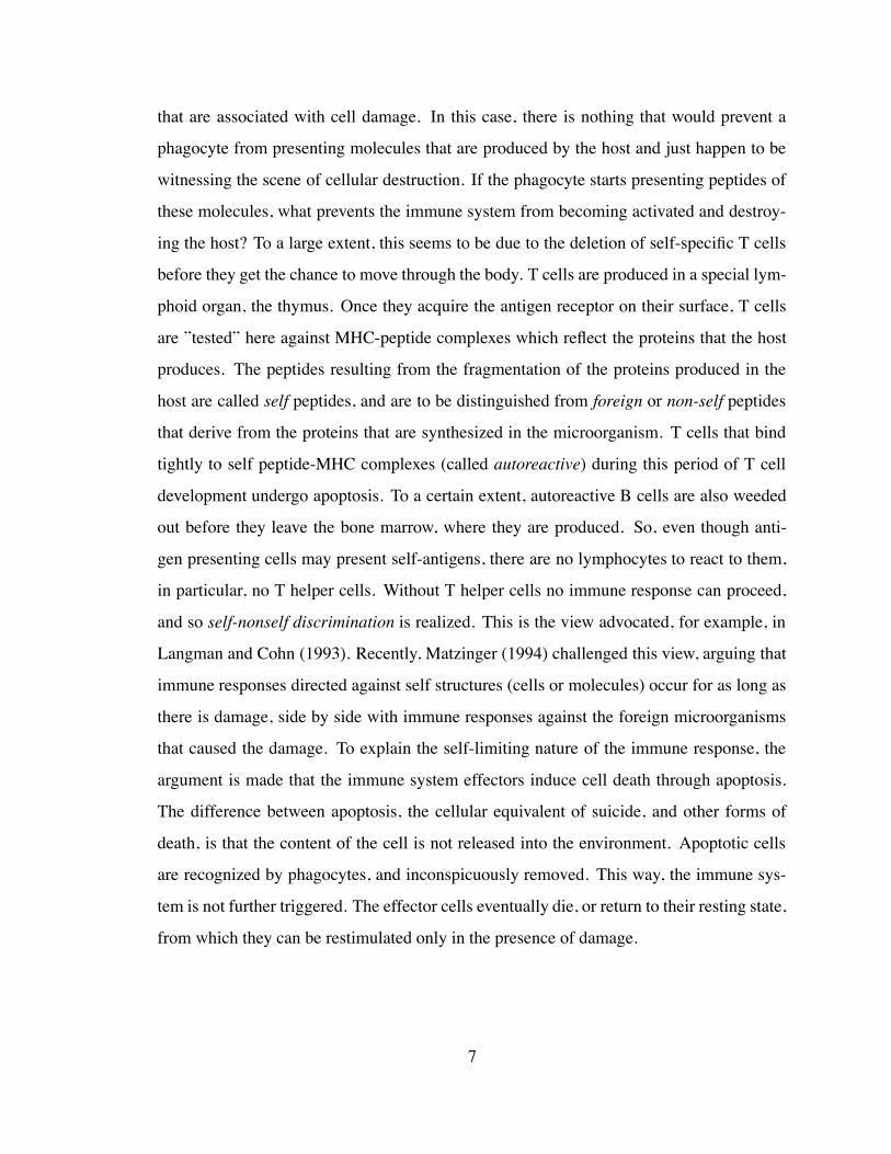
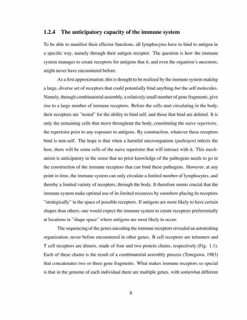
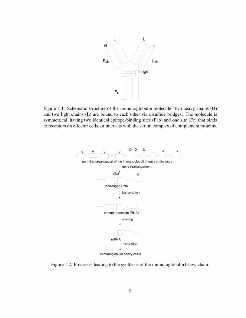
Figure 1.1: Schematic structure of the immunoglobulin molecule: two heavy chains (H)and two light chains (L) are bound to each other via disulfide bridges. The molecule issymmetrical, having two identical epitope-binding sites (Fab) and one site (Fc) that bindsto receptors on effector cells, or interacts with the serum complex of complement proteins.

V V V VD D D JJ C

germline organization of the immunoglobulin heavy chain locus

rearranged DNA

VDJ C

primary transcript (RNA)

mRNA

immunoglobulin heavy chain

gene rearrangement

transcription

splicing

translation

Figure 1.2: Processes leading to the synthesis of the immunoglobulin heavy chain.

9

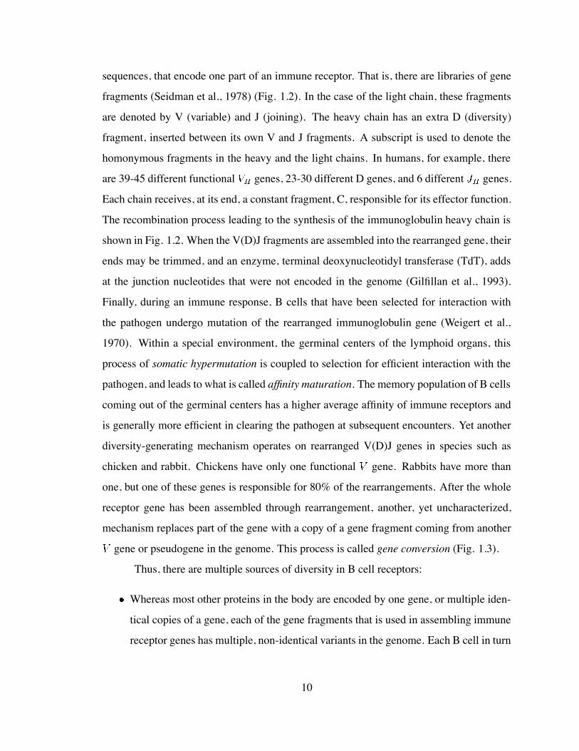
sequences, that encode one part of an immune receptor. That is, there are libraries of gene

fragments (Seidman et al., 1978) (Fig. 1.2). In the case of the light chain, these fragments

are denoted by V (variable) and J (joining). The heavy chain has an extra D (diversity)

fragment, inserted between its own V and J fragments. A subscript is used to denote the

homonymous fragments in the heavy and the light chains. In humans, for example, there

are 39-45 different functional genes, 23-30 different D genes, and 6 different genes.

Each chain receives, at its end, a constant fragment, C, responsible for its effector function.

The recombination process leading to the synthesis of the immunoglobulin heavy chain is

shown in Fig. 1.2. When the V(D)J fragments are assembled into the rearranged gene, their

ends may be trimmed, and an enzyme, terminal deoxynucleotidyl transferase (TdT), adds

at the junction nucleotides that were not encoded in the genome (Gilfillan et al., 1993).

Finally, during an immune response, B cells that have been selected for interaction with

the pathogen undergo mutation of the rearranged immunoglobulin gene (Weigert et al.,

1970). Within a special environment, the germinal centers of the lymphoid organs, this

process of somatic hypermutation is coupled to selection for efficient interaction with the

pathogen, and leads to what is called affinity maturation. The memory population of B cells

coming out of the germinal centers has a higher average affinity of immune receptors and

is generally more efficient in clearing the pathogen at subsequent encounters. Yet another

diversity-generating mechanism operates on rearranged V(D)J genes in species such as

chicken and rabbit. Chickens have only one functional gene. Rabbits have more than

one, but one of these genes is responsible for 80% of the rearrangements. After the whole

receptor gene has been assembled through rearrangement, another, yet uncharacterized,

mechanism replaces part of the gene with a copy of a gene fragment coming from another

gene or pseudogene in the genome. This process is called gene conversion (Fig. 1.3).

Thus, there are multiple sources of diversity in B cell receptors:

Whereas most other proteins in the body are encoded by one gene, or multiple iden-

tical copies of a gene, each of the gene fragments that is used in assembling immune

receptor genes has multiple, non-identical variants in the genome. Each B cell in turn

10

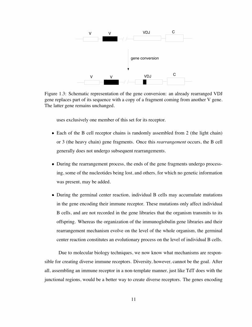
gene conversion

V V VDJ C

V V VDJ C

Figure 1.3: Schematic representation of the gene conversion: an already rearranged VDJgene replaces part of its sequence with a copy of a fragment coming from another V gene.The latter gene remains unchanged.

uses exclusively one member of this set for its receptor.

Each of the B cell receptor chains is randomly assembled from 2 (the light chain)

or 3 (the heavy chain) gene fragments. Once this rearrangement occurs, the B cell

generally does not undergo subsequent rearrangements.

During the rearrangement process, the ends of the gene fragments undergo process-

ing, some of the nucleotides being lost, and others, for which no genetic information

was present, may be added.

During the germinal center reaction, individual B cells may accumulate mutations

in the gene encoding their immune receptor. These mutations only affect individual

B cells, and are not recorded in the gene libraries that the organism transmits to its

offspring. Whereas the organization of the immunoglobulin gene libraries and their

rearrangement mechanism evolve on the level of the whole organism, the germinal

center reaction constitutes an evolutionary process on the level of individual B cells.

Due to molecular biology techniques, we now know what mechanisms are respon-

sible for creating diverse immune receptors. Diversity, however, cannot be the goal. After

all, assembling an immune receptor in a non-template manner, just like TdT does with the

junctional regions, would be a better way to create diverse receptors. The genes encoding

11

immune receptors are carrying some information, and what that information might be is

the question that stirred my interest.

1.2.5 Structural components of the immune receptors

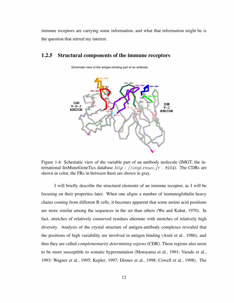
Schematic view of the antigen-binding part of an antibody

Figure 1.4: Schematic view of the variable part of an antibody molecule (IMGT, the in-ternational ImMunoGeneTics database ). The CDRs areshown in color, the FRs in between them are shown in gray.

I will briefly describe the structural elements of an immune receptor, as I will be

focusing on their properties later. When one aligns a number of immunoglobulin heavy

chains coming from different B cells, it becomes apparent that some amino acid positions

are more similar among the sequences in the set than others (Wu and Kabat, 1970). In

fact, stretches of relatively conserved residues alternate with stretches of relatively high

diversity. Analysis of the crystal structure of antigen-antibody complexes revealed that

the positions of high variability are involved in antigen binding (Amit et al., 1986), and

thus they are called complementarity determining regions (CDR). These regions also seem

to be more susceptible to somatic hypermutation (Motoyama et al., 1991; Varade et al.,

1993; Wagner et al., 1995; Kepler, 1997; Dorner et al., 1998; Cowell et al., 1998). The

12

more conserved regions are packed inside the molecule or are involved in the pairing of

the heavy and light chains (Foote and Winter, 1992). They are called framework regions

(FR). The V gene fragment is responsible for encoding FR1, CDR1, FR2, CDR2, and part

of the CDR3. The J gene fragment encodes part of CDR3 and FR4. In heavy chains, the D

gene fragment also contributes to CDR3. Fig. 1.4 shows the variable part of an antibody

molecule, with the CDRs that are contributed to the binding site by both heavy and light

chains. The C fragment, that encodes the constant part of the immune receptor and is

responsible for the effector functions is shown in Fig. 1.1.

A comparative analysis of the immune repertoire in various species, and in various

developmental stages of an organism, reveals that there is a lot of variability in the way

the repertoire is created. The diversity of region genes that are present in the germline

can vary considerably. In sharks, all genes are more than 90% homologous, whereas

in mice and humans the pairwise homology between these genes can be as low as 70%.

In neonates, the combinatorial and junctional diversity seem to be circumvented (Feeney,

1992). Preferential V-D and D-J joining could reduce the repertoire to a relatively small

set of germline-encoded antibodies. In sharks, we encounter the extreme of this spectrum

(Hinds-Frey et al., 1993). A large fraction of their antibody genes are already joined in

germline, with no possibility of combinatorial diversification. The light chain-heavy chain

pairing is abolished in camel IgM homodimers. The absence of TdT in genetically manipu-

lated mice does not visibly affect their survival chances (Gilfillan et al., 1993). All this data

argues that combinatorial diversity might not be indispensable for survival. Two features,

however, seem to characterize all the immune systems encountered in nature: An organism

has multiple genes that encode immune receptors; A secondary diversification mechanism

is always found, and generally that mechanism is somatic hypermutation. In the following

chapters, I will present a number of models that I used to explore the contribution of the

germline diversity and somatic hypermutation to the immune repertoire. I will argue that

the naive repertoire is likely to realize a coarse-graining of the pathogen space, with somatic

hypermutation being required for improving the affinity/specificity of the antigen-selected

13

antibodies. I will also analyze the factors that contribute to the efficiency of somatic hyper-

mutation.

14

Chapter 2

How much can germline diversity do?

An immune receptor gene is assembled from a number of gene fragments. Each of the

fragments comes from a gene library, and only one member of each of the gene libraries

is used for a given immune receptor. The fragment is the largest of the two (or three,

in the case of the antibody heavy chain and T cell receptor chain), with a length of

approximately 100 amino acids. What shapes the evolution of the immune receptor libraries

is largely unknown. Given that epidemics have been an important selection pressure in the

evolution of human populations we expect that the these gene libraries bear the traces of

the antigenic exposures of the species. On the other hand, immune responses to artificially-

produced molecules have been induced in mice, suggesting that the immune system is able

to recognize more than the antigens that the species encountered in its evolution. These

observations lead to the idea that the immune system creates its receptors so as to be able

to recognize as many molecular shapes as possible. Was the immune system evolved in

such a way, or does it only focus on the molecular shapes that are most detrimental to the

survival chance of the organism?

In the following section I will explore the scaling between the fitness of the organism–

defined as its probability to survive in a pathogenic environment–and the size of its anti-

body repertoire. I will argue that the functional form of this dependency suggests that

the role of germline diversity must be to broadly map the regions of the pathogen space

15

that are relevant for the survival of the organism. Moreover, I will argue that biases in

the pathogen exposure of the individuals, such as sampling the pathogen universe, would

preclude the evolution of germline-encoded antibodies that optimally cover the complete

space of molecular shapes. Thus, contrary to what is commonly believed, I argue that the

immune system does not handle as many molecular shapes as possible. It rather focusses on

those that have been important for the survival of the species. Responses to artificially con-

structed molecules are possible because these molecules are sufficiently similar to epitopes

that are encountered on pathogens.

2.1 Shape space coveragewith distance-dependentmatch-

ing

The concept of a shape space was introduced by Perelson and Oster (1979). Since then, it

has been used in numerous theoretical studies of the immune system, of which I will only

mention a few (Perelson, 1989; Segel and Perelson, 1989; De Boer et al., 1992; Detours

et al., 1994). In this framework, it is postulated that molecular interactions can be under-

stood in terms of the ”shape” of the molecules. The crucial assumption of this model is

that the ”shape” of a molecule can be represented by a vector of discrete values, from a

finite, generally small, alphabet. Rules are specified for determining the ”affinity” between

two such ”shapes”. There have been attempts to relate this model to measurements that

can be obtained in biological systems As (B-Rao and Stewart, 1996; Smith et al., 1997). I

therefore decided to use this conceptualization for my study on the evolution of antibody

gene libraries.

It is generally assumed that the number of pathogens in the environment of a species

is very large. Indeed, if this number was small, the immune system would be able to

distribute its resources, such as antibody molecules, among these pathogens. Each of the

pathogens would raise an effective immune response. This is clearly not what we observe

in reality. Therefore, I will assume that the pathogen universe is large. One has to keep

16

in mind, though, that the failure of the immune system to cope with all the pathogenic

challenges that it encounters may be due to other factors. Pathogen evolution sets a moving

target for the immune system. As I will show in the following section, the rate at which the

antibody library adapts to an evolving pathogenic environment might be too slow for the

immune system to ever pin down even a small pathogen set.

Let us assume that the number of antibody shapes encoded in the genome is con-

siderably smaller than the number of antigen shapes that the organism encounters during

its life time. To understand the role of the antibody gene libraries in the generation of the

immune repertoire, I will address the following questions:

How does the survival probability of the organism scale with the size of its immune

receptor repertoire?

What structure do antibody libraries evolve in different types of pathogenic environ-

ments?

Can an antibody repertoire that has been selected for interaction with pathogens per-

form equally well in the interaction with non-pathogenic antigens?

2.1.1 Model

To address these questions, I implemented an evolutionary algorithm, similar to the one

introduced by Hightower (1996). The basic components of the model are the following:

A population of individuals, each having a gene library of genes. Each gene is

represented by a bit string of length . From this library, I assume that antibodies

are made, that is, all genes are expressed, and that all these antibodies are available for

binding any of the pathogens. I do not distinguish between the genotype (antibody

gene) and the phenotype (antibody molecule). One could, alternatively, view the

libraries as representing the possible set of antibodies that an organism can produce.

The genetic operators, to be discussed below, such as mutation and recombination

17

on these libraries would then have to be thought to represent phenotypic changes to

the antibody repertoire as a result of implicit genetic operations on the level of the

genes. Also, I will not include the rearrangement process in the model. This choice

is meant mainly to keep the model simple. Note, immune receptor rearrangement

does not play a major role in generating diversity in all species, and thus the simple

model that I propose has direct significance for these situations.

Pathogens are also represented as bit strings of length .

The essence of the complicated antibody-pathogen interaction in the real world, that

I want to capture in this model, is that for each pathogen in the environment, the

host can raise at least one antibody that can recognize the pathogen. The level of

recognition may or may not be protective for the individual. As suggested recently

(Dal Porto et al., 1998), I will not require a certain affinity threshold for protection.

I will simply assume that the lower the affinity, the lower the survival chances when

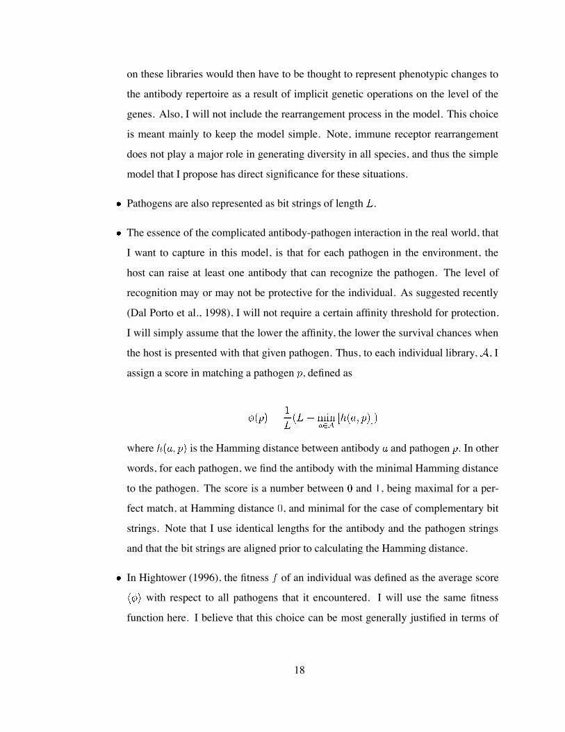
the host is presented with that given pathogen. Thus, to each individual library, , I

assign a score in matching a pathogen , defined as

where is the Hamming distance between antibody and pathogen . In other

words, for each pathogen, we find the antibody with the minimal Hamming distance

to the pathogen. The score is a number between and , being maximal for a per-

fect match, at Hamming distance , and minimal for the case of complementary bit

strings. Note that I use identical lengths for the antibody and the pathogen strings

and that the bit strings are aligned prior to calculating the Hamming distance.

In Hightower (1996), the fitness of an individual was defined as the average score

with respect to all pathogens that it encountered. I will use the same fitness

function here. I believe that this choice can be most generally justified in terms of

18

the survival probabilities of an individual with respect to the pathogen challenges it

encounters. All these challenges have to be met successfully if the organism is to

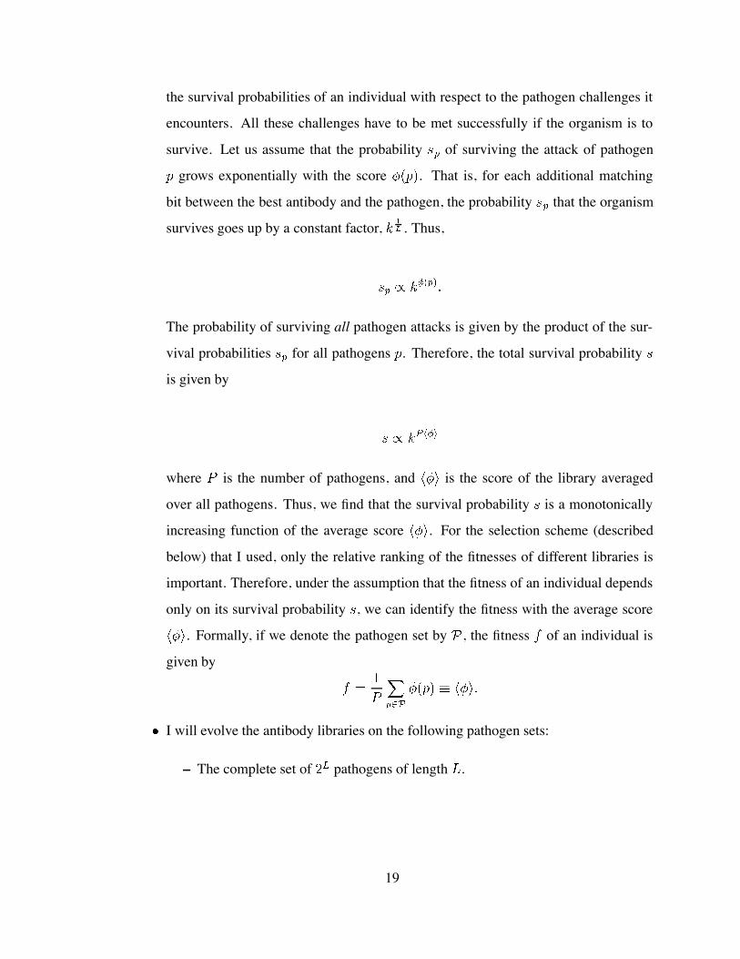
survive. Let us assume that the probability of surviving the attack of pathogen

grows exponentially with the score . That is, for each additional matching

bit between the best antibody and the pathogen, the probability that the organism

survives goes up by a constant factor, . Thus,

The probability of surviving all pathogen attacks is given by the product of the sur-

vival probabilities for all pathogens . Therefore, the total survival probability

is given by

where is the number of pathogens, and is the score of the library averaged

over all pathogens. Thus, we find that the survival probability is a monotonically

increasing function of the average score . For the selection scheme (described

below) that I used, only the relative ranking of the fitnesses of different libraries is

important. Therefore, under the assumption that the fitness of an individual depends

only on its survival probability , we can identify the fitness with the average score

. Formally, if we denote the pathogen set by , the fitness of an individual is

given by

I will evolve the antibody libraries on the following pathogen sets:

– The complete set of pathogens of length .

19

– Random subsets of the complete pathogen set of size . These sets are

constructed by sampling pathogens, with replacement, from the complete

pathogen set.

– Pathogen sets that evolve independently of the hosts.

The evolutionary algorithm that I used has the following structure. The initial popu-

lation consists of random libraries, of identical size, . This population size

is sufficiently large to allow convergence to relatively high fitness solutions, given the

mutation rate of per bit that I used in evolving the libraries. Each individual,

then, consists of a single library. I use rank selection as follows: If is the rank of the

fitness of an individual in the population, the chance of that individual being selected

as a parent is, on average, . To create one library of the new generation,

I select, with replacement, two libraries of the old population, then generate two new

libraries by crossing over the two chosen libraries. The number of crossover points

is chosen from a binomial distribution with mean . This crossover scheme is

more realistic for our purpose of modeling the evolution of gene libraries than other

schemes that are described in the evolutionary algorithms literature (Mitchell, 1996).

The crossover points are chosen at the boundary between antibodies, so individual

antibodies are not disrupted by crossover. I then choose one of the new crossover

products, mutate it, and add it to the new population. 1000 generations of the ge-

netic algorithm constitute a run. At the end of the run, I take the library with the

highest fitness in the population, and use it to infer the scaling relation, as well as for

analyzing the properties of antibodies that were evolved.

A note about the random number streams. The basic function of the random number

stream returns a random deviate from a uniform distribution on the interval [0,1). The

algorithm is given in Knuth (1973), and the implementation that I used was written by

Terry Jones. This function can be used to generate random deviates of the uniform density

function over any interval between 0 and any positive value.

20

2.1.2 Lower bound on the evolved fitness

The performance of a random library should give us a lower bound on the fitness of evolved

libraries, given that I start the simulation with random antibody libraries. I therefore de-

rived the expected fitness of a random library on the complete pathogen set of size . Let

be the score of an individual with respect to pathogen and the number of match-

ing bit positions between a pathogen and an antibody. For a pathogen binding to a single

random antibody, the probability that there are or fewer matching bits, , is

given by the value of the cumulative binomial at . If we have random antibodies, the

probability that all of them have or fewer matching bit positions with the pathogen is

. Then the probability that the score of the individual with respect to

pathogen is , is given by the probability that at least one antibody has matching

sites with the pathogen but none has more than , i.e.,

The expected score of a random library of antibodies with a random pathogen is then

given by

The expected score of a random library on a randomly chosen pathogen also represents

the expected score of a random library over the complete set of pathogens. We then

denote the expected fitness of a random library over the complete pathogen set by ,

(2.1)

The above equation for gives a lower bound on the fitness of the evolved libraries as a

function of and .

2.1.3 Upper bound on the evolved fitness

I also calculate an upper bound for the fitness of the evolved libraries by using a theorem

from the theory of error-correcting codes (MacWilliams and Sloane, 1986). Assume that

21

we distribute the antibodies over the space of pathogen bit strings in such a way that

each antibody covers a set of volume , corresponding to the number of pathogens

up to Hamming distance from antibody . Assume that all sets are disjoint and of

equal size. In the best situation, there exists a Hamming distance such that the sets

together exactly cover the space of pathogens. Since

this yields the inequality

(2.2)

In the theory of error-correcting codes, this inequality is known as the sphere-packing or

Hamming bound. The library is ”perfect” if equality holds. The fitness of such a perfect

library is given by

However, it may be that a ”perfect” library cannot be constructed. That is, there is no value

of for which the disjoint Hamming distance -balls around the antibodies cover the

space completely. In this situation, we first determine the maximum value of for which

the inequality 2.2 still holds. Each antibody will cover a ball of pathogens around itself, up

to Hamming distance . The rest of the pathogen strings, that do not fall in any of the

Hamming distance -balls around the antibodies, will be at Hamming distance from

at least one of the antibodies. Thus, given this value , the upper bound on the fitness will

be given by

2.1.4 The fitness of evolved libraries

How does the fitness of the evolved libraries compare to the bounds that we calculated?

I used a string length bits to explore the scaling relation between the maxi-

mum fitness evolved by a library and the number of antibodies, , in the library. The fitness

22

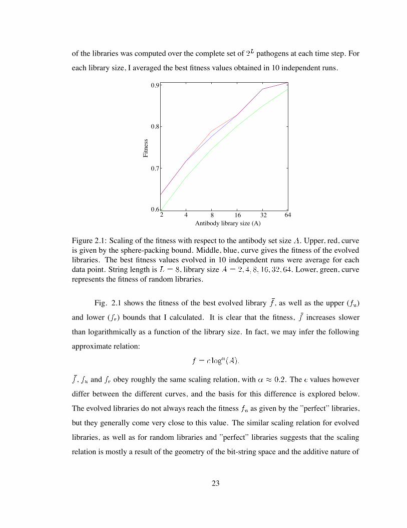
of the libraries was computed over the complete set of pathogens at each time step. For

each library size, I averaged the best fitness values obtained in 10 independent runs.

2 4 8 16 32 640.6

0.7

0.8

0.9

Antibody library size (A)

Fitn

ess

Figure 2.1: Scaling of the fitness with respect to the antibody set size . Upper, red, curveis given by the sphere-packing bound. Middle, blue, curve gives the fitness of the evolvedlibraries. The best fitness values evolved in 10 independent runs were average for eachdata point. String length is , library size . Lower, green, curverepresents the fitness of random libraries.

Fig. 2.1 shows the fitness of the best evolved library , as well as the upper ( )

and lower ( ) bounds that I calculated. It is clear that the fitness, increases slower

than logarithmically as a function of the library size. In fact, we may infer the following

approximate relation:

, and obey roughly the same scaling relation, with . The values however

differ between the different curves, and the basis for this difference is explored below.

The evolved libraries do not always reach the fitness as given by the ”perfect” libraries,

but they generally come very close to this value. The similar scaling relation for evolved

libraries, as well as for random libraries and ”perfect” libraries suggests that the scaling

relation is mostly a result of the geometry of the bit-string space and the additive nature of

23

the matching rule.

Thus to obtain an increase of in fitness one would have to multiply the size of

the libraries by larger and larger factors. The selection pressure for increasing the size

of the germline-encoded repertoire is thus expected to be progressively lower. A similar

dependency was suggested, on experimental grounds, and within a somewhat different

model, by Minar (1994).

2.1.5 The strategy of evolved libraries

What strategy do the relatively small antibody libraries evolve for matching the much larger

set of pathogens? If the pathogen set was small, we would expect that the antibodies evolve

to track the pathogens perfectly. Thus, in the structure of the antibody library will directly

reflect the structure of the pathogen set. What we do not know is what strategies these

libraries develop when confronted with a pathogen set much larger than the size of the li-

brary, or with a very dynamical pathogen set. In the first scenario, it would be impossible to

track pathogens individually. In the second scenario, the ability to track pathogens individ-

ually probably depends on the relative rate of evolution of the pathogens on one hand, and

the antibody library, on the other. To investigate the type of library structure that evolves in

these cases, I performed the following evolutionary algorithm experiments.

The set of all bit strings will be denoted as the pathogen universe. A subset of

it will be used for training the antibody libraries. I call this the training set. For a length

of antibody and pathogen bit strings, I generated, with replacement, training sets

of size 2, 4, 8, 16, 32, 64, 128, 256, 512, 1024, 4096, and 16384. Using these sets, I then

evolved gene libraries of size , as previously described. I further investigated two

types of pathogen dynamics. These are meant to correspond to:

1. pathogenic environments that change from one generation of hosts to another, and

2. individual pathogens slowly drifting in the molecular shape space.

I simulated the first type of dynamics by replacing of the training set at generation

24

of hosts. The second type of dynamics I implemented by mutating each pathogen in the

training set with 0.1 probability per pathogen per generation of hosts. The exact values of

these parameters are arbitrary. The intent, however, is not to give quantitative predictions,

but to understand the qualitative behavior of the libraries under the two types of pathogen

dynamics.

To assess library structure, I use an observation of Hightower (1996). Investigating

the type of library that evolves when the pathogen set is very large, the author conjectured

that the antibodies tend to maximize the average Hamming distance to other antibodies in

the library. I can, in fact determine what this distance will be, and then ask whether this

strategy is employed both by libraries that evolve in large, static pathogenic environments,

as well as in small, rapidly changing pathogenic environments.

The average pairwise Hamming distance within a library is given by

where is the number of antibodies in the library, and and are individual antibodies.

The Hamming distance between two antibodies, is given by:

where and denotes the bit position of the two strings, and

if

otherwise

We may now switch the order of summations to obtain:

and since the bits are independent, maximizing this quantity means maximizing the pair-

wise Hamming distance at each bit position. If for bit position we denote by the

frequency of 0’s in the antibody population at that position, then the pairwise Hamming

25

distance at that position is . This quantity is maximal for . Substi-

tuting into the above equation, we obtain the maximal average Hamming distance in the

population:

For libraries of 8 antibodies of length 16, the average pairwise Hamming distance between

the antibodies in the library would have to be 9.1429. Let us now return to the two types

of pathogenic environments: a static, large, training set (of size ), and a small

training set (size ), with one pathogen being replaced by a random other at each

generation of hosts. All 5 libraries evolved on the large, static training set had an average

pairwise Hamming distance of 9, whereas in 9 out of 10 libraries evolved with dynamic

training set, the average pairwise Hamming distance in the library was 8 (in the 1 other

case it was 7). To determine the significance of this difference, I constructed random

libraries of 8 antibodies, and calculated the average pairwise Hamming distance in each

of these libraries. I used these values to construct the distribution of average pairwise

Hamming distance for random libraries. It is not surprising that the libraries that were

evolved on small, dynamic, training set cannot be distinguished (using the average pairwise

Hamming distance statistic) from random libraries. On the other hand, the libraries evolved

on large, static training sets have significantly higher average pairwise Hamming distance

than random libraries of the same size ( ). I thus conclude that a

small, dynamic training set does not allow the antibodies to distribute themselves in space

such as to optimally cover the pathogen universe.

Though having maximal average Hamming distance between the genes in the library

seems to be a necessary condition for maximal fitness, it is not sufficient. Clearly, a library

of size composed of four copies of a string and four copies of its complement has

maximal average pairwise Hamming distance, but it is far from being optimal. It is unclear

what other condition needs to be fulfilled for a library to achieve maximal fitness.

Let us return now to the question of whether the libraries learn to recognize the

26

8 32 128 512 4096 655360.67

0.68

0.69

0.7

training set size

expe

cted

fitn

ess t

o a

rand

om p

atho

gen

Figure 2.2: Expected fitness of evolved libraries with respect to a random pathogen, as afunction of the training set size. The libraries that were evaluated are the ones evolved onstatic training set (red), slowly changing training set (green), rapidly changing training set(blue).

pathogens on which they have been trained, or they evolve such as to maximize recognition

of a random molecular shape. I used the libraries that I evolved in the experiments described

above to determine their expected fitness to a random shape in the universe. That is, I

determined the average fitness of the libraries on all pathogen bit strings of length .

Fig. 2.2 shows the results. For static training sets (upper curve) 100 runs were used

for training set sizes 8, 16, 32, 64; 50 runs for training set sizes 128 and 256; 25 runs for

training set size 512; 10 runs for training set size 1024, and 5 runs for training set size

4096, and 16384. For changing training set, 10 runs were performed for each training set

size, with the exception of the training set size of 4096, for which 6 runs were used. As the

figure shows, the most important determinant of the fitness relative to a random pathogen

is the fraction of the pathogen universe that a host encounters in one generation. If this

fraction is large, fitness of evolved library is high, independent of the pathogen dynamics.

This is not surprising. In the limit of the training set being the pathogen universe itself,

these scenarios are indistinguishable. Libraries evolved on small, but variable training sets

27

have lower performance on a random pathogen than libraries that evolved on large and

static training sets (or large, but dynamic pathogen sets). This shows that the small, dy-

namic, pathogenic environments do not allow optimal placement of antibodies in the space

of molecular shapes. On the other hand, the libraries that evolve in environments with few

pathogens have a higher expected performance on random pathogens if the environment

in which the libraries evolve is dynamic. The reason is that the static environment sup-

ports the evolution of very specialized libraries, while the dynamic environment essentially

maintains random antibody libraries. A somewhat similar idea was reported by Hightower

(1996), who found that stochastic antibody expression induces libraries that are more robust

in handling a random pathogen.

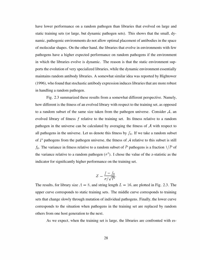
Fig. 2.3 summarized these results from a somewhat different perspective. Namely,

how different is the fitness of an evolved library with respect to the training set, as opposed

to a random subset of the same size taken from the pathogen universe. Consider , an

evolved library of fitness relative to the training set. Its fitness relative to a random

pathogen in the universe can be calculated by averaging the fitness of with respect to

all pathogens in the universe. Let us denote this fitness by . If we take a random subset

of pathogens from the pathogen universe, the fitness of relative to this subset is still

. The variance in fitness relative to a random subset of pathogens is a fraction of

the variance relative to a random pathogen ( ). I chose the value of the z-statistic as the

indicator for significantly higher performance on the training set.

The results, for library size , and string length , are plotted in Fig. 2.3. The

upper curve corresponds to static training sets. The middle curve corresponds to training

sets that change slowly through mutation of individual pathogens. Finally, the lower curve

corresponds to the situation when pathogens in the training set are replaced by random

others from one host generation to the next.

As we expect, when the training set is large, the libraries are confronted with es-

28

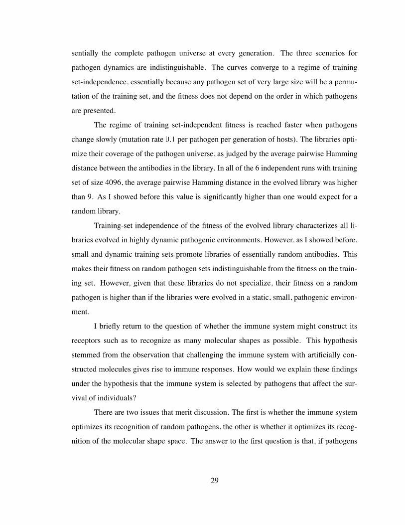
sentially the complete pathogen universe at every generation. The three scenarios for

pathogen dynamics are indistinguishable. The curves converge to a regime of training

set-independence, essentially because any pathogen set of very large size will be a permu-

tation of the training set, and the fitness does not depend on the order in which pathogens

are presented.

The regime of training set-independent fitness is reached faster when pathogens

change slowly (mutation rate per pathogen per generation of hosts). The libraries opti-

mize their coverage of the pathogen universe, as judged by the average pairwise Hamming

distance between the antibodies in the library. In all of the 6 independent runs with training

set of size 4096, the average pairwise Hamming distance in the evolved library was higher

than 9. As I showed before this value is significantly higher than one would expect for a

random library.

Training-set independence of the fitness of the evolved library characterizes all li-

braries evolved in highly dynamic pathogenic environments. However, as I showed before,

small and dynamic training sets promote libraries of essentially random antibodies. This

makes their fitness on random pathogen sets indistinguishable from the fitness on the train-

ing set. However, given that these libraries do not specialize, their fitness on a random

pathogen is higher than if the libraries were evolved in a static, small, pathogenic environ-

ment.

I briefly return to the question of whether the immune system might construct its

receptors such as to recognize as many molecular shapes as possible. This hypothesis

stemmed from the observation that challenging the immune system with artificially con-

structed molecules gives rise to immune responses. How would we explain these findings

under the hypothesis that the immune system is selected by pathogens that affect the sur-

vival of individuals?

There are two issues that merit discussion. The first is whether the immune system

optimizes its recognition of random pathogens, the other is whether it optimizes its recog-

nition of the molecular shape space. The answer to the first question is that, if pathogens

29

-2

0

2

4

8

6

10

12

14

z

8 32 128 512 4096 65536training set size

Figure 2.3: Dependence of the z-statistic on the training set size . The size of the antibodylibrary was kept constant, genes. Length of antibody and pathogen strings isbits. The three data sets are, from top to bottom, static pathogen set, slowly mutatingpathogen set, rapidly changing pathogen set. The number of independent runs for eachpathogen set size is given in the text.

are independent from one another, the immune system needs to be presented with a large

fraction of the pathogen universe at each generation to be able to optimize its recognition

of random pathogens. This fraction is somewhat lower if pathogens also evolve from one

generation of hosts to the next (the condition that the pathogen set is considerably larger

than the antibody libraries still has to be maintained).

Regarding the recognition of the molecular shape space, we would probably need

to do the following experiment. Assuming that the pathogen universe is a fraction of the

molecular shape space, we may distribute the pathogens in the space in different ways. The

two extremes are:

We choose a random point in the space, and then progressively add its neighbors,

in increasing order of the Hamming distance, until we reach a pathogen set size of

.

We construct the pathogen set by choosing, with probability , each of the points

30

of the molecular space.

We expect that the antibodies that will evolve in these two situations would have very

different performance on a random molecular shape. Namely, the recognition of a random

molecular shape will be higher if the pathogens are scattered through the space.

2.2 Shape space coverage with other matching rules

Although the concept of a shape space has spun numerous studies on the behavior and

evolution of the immune system, it is not clear that intermolecular interactions are well

described in this manner. In fact, a survey of the literature also reveals discussions of the

relevance of the shape-space model, at least in idiotypic interactions (Carneiro and Stewart,

1994). I therefore decided to investigate the impact of another fitness function on the basic

scaling result that I obtained above. The fitness function that stems from the shape-space

metaphor is highly structured, the fitness of an individual being given by the antibody with

the smallest Hamming distance from the pathogen. We would like to know what happens

if the fitness landscape has a completely different structure. The option I explore is based

on the idea of a random energy model, introduced by Derrida (1984),in the context of

spin-glasses.

If we view the antigen-antibody interaction from a biochemical standpoint, the

strength of the bond is given by the difference of the free energies of the complex, and of

the two molecules in their unbound state. A realistic representation of the energy landscape

as a function of the sequence of the molecules is clearly impossible at this point. There-

fore I use the following abstraction. I assume that each molecule has an ”energy”, which

is a random deviate from a Gaussian distribution. The antigen-antibody complex also has

an energy corresponding to it, which is a random deviate of a Gaussian distribution. The

difference between the energy of the complex and the energy of unbound molecules gives

the strength of the bond between them. I perform this calculation for all antibodies that the

individual can make, and I take the maximum bond strength between an antibody and the

31

pathogen to be the fitness with respect to that pathogen. I then use the evolutionary algo-

rithm that I described in section 2.1.1 to evolve libraries of different sizes on a complete

pathogen set of size . As the bit-strings that I used have length , the

7 high order bits are set to 0. The best library evolved in 1000 steps is used to infer the

scaling relation between fitness and antibody library size.

The energy of antigens and antibodies is drawn from a Gaussian distribution with

mean 50, and variance 2.5, whereas the energy of the complex was chosen from a Gaussian

distribution with mean 100 and variance 10. Although the exact choice of the mean and

variance of the energy of an individual molecule is arbitrary, there clearly is a scaling

of the energy of a molecule with its size, so we expect that by doubling the size of the

molecule we roughly double the energy associated with it. To determine the energy of each

molecule, I seed the random number generator with the numerical representation of the bit

string representing that molecule, and then calculate a pseudo-random Gaussian deviate

according to the algorithm given in Press et al. (1988). I assign such an energy to both

antigen and antibody. To obtain the antigen-antibody complex, I take the XOR between the

bit strings representing the antigen and the antibody. I use the numerical representation of

this bit string to calculate an energy, as described above. The bond strength, given by the

difference in energy between the complex and the unbound molecules, will be distributed

as a Gaussian with mean 0 and variance 15.

One might argue that the landscape thus constructed does not have any obvious

structure for the evolutionary algorithm to work with, given that the energies assigned to

closely related genotypes are random deviates from the Gaussian distribution. The land-

scape does, however, have some structure, as the antibodies with high energy have a better

chance of lowering this energy by binding to pathogens. These are, in fact, the antibodies

that the evolutionary algorithm discovers.

In the previous section I showed that, for the shape space model, the scaling relation

between fitness and library size in the case of evolved libraries is essentially a shifted

variant of the relation that we obtain for a random library of identical size. I will show that

32

this is also the case for the energy model that I just described.

2.2.1 Lower bound on the fitness

Let us first determine the fitness of a random library as a function of the library size. I will

write the derivation in the most general sense, in terms of the density distribution of the

bond strength, , and its corresponding cumulative density function, , and I will

apply it to the particular Gaussian distribution of bond strengths that I mentioned above.

For every pathogen, the fitness is given by the maximum of random variables

drawn from the distribution , being the size of the antibody library. The probability

that the bond strength between a random pathogen and all of the antibodies in the library

is less than or equal to a value, , is , and then the derivative of this, giving the

probability density of fitness , is

(2.3)

Now the expected fitness of a random library of antibodies on the complete pathogen

space, given the probability density function of the fitness, , is

(2.4)

Let , taking values between 0 and 1. Then and Eq. 2.4 can be

rewritten in terms of as

(2.5)

where denotes the fact that has to be expressed now as a function of . But

, thus , and , where denotes the inverse

function of . With this, Equation 2.5 becomes

(2.6)

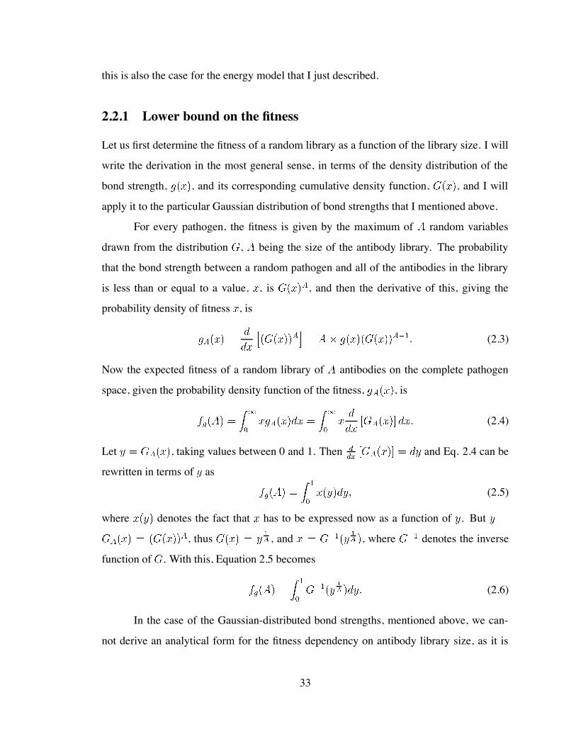
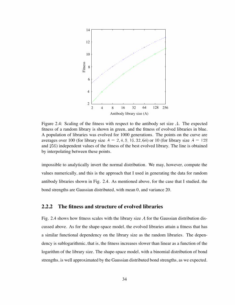
In the case of the Gaussian-distributed bond strengths, mentioned above, we can-

not derive an analytical form for the fitness dependency on antibody library size, as it is

33

2

4

6

8

10

12

14

2 4 8 16 32 64 128 256Antibody library size (A)

Fitn

ess

Figure 2.4: Scaling of the fitness with respect to the antibody set size . The expectedfitness of a random library is shown in green, and the fitness of evolved libraries in blue.A population of libraries was evolved for 1000 generations. The points on the curve areaverages over 100 (for library size ) or 10 (for library sizeand ) independent values of the fitness of the best evolved library. The line is obtainedby interpolating between these points.

impossible to analytically invert the normal distribution. We may, however, compute the

values numerically, and this is the approach that I used in generating the data for random

antibody libraries shown in Fig. 2.4. As mentioned above, for the case that I studied, the

bond strengths are Gaussian distributed, with mean 0, and variance 20.

2.2.2 The fitness and structure of evolved libraries

Fig. 2.4 shows how fitness scales with the library size for the Gaussian distribution dis-

cussed above. As for the shape-space model, the evolved libraries attain a fitness that has

a similar functional dependency on the library size as the random libraries. The depen-

dency is sublogarithmic, that is, the fitness increases slower than linear as a function of the

logarithm of the library size. The shape-space model, with a binomial distribution of bond

strengths, is well approximated by the Gaussian distributed bond strengths, as we expected.

34

Let us analyze the structure of the evolved libraries. Given the fitness function that

we used, we would expect that antibodies that have a high free energy in the unbound

state would have the highest chance of lowering their free energy through intermolecular

binding. It turns out that the evolved antibodies have higher than average energy. To assess

the significance of this difference, we calculate the z-statistic for the evolved antibodies,

that is where is the energy of an evolved antibody, is the mean energy

of an antibody molecule, and is the standard deviation of the energy of an antibody

molecule. The evolved antibodies have a z-statistic centered around 2 standard deviations

higher than the mean, clearly different from the mean. What this result tell us is that, as

expected, the antibodies that were evolved are the equivalent of the ”sticky” antibodies, of

high interconnectivity and multispecificity, such as those commonly seen in the immune

systems of newborns (see for example Kearney et al. (1992)). These antibodies bind not

only to pathogens, but to many other molecules normally present in the body, including

DNA and molecules on the surface of lymphoid cells. Thus, the evolutionary algorithm

was able to evolve a property known to characterize the immune systems of newborns.

2.2.3 Implications for random antibody libraries

Although I do not have a formal proof, it seems that evolving the antibody libraries allows

us to reach higher fitness values than we would have with random libraries, though the

functional form of the dependency between fitness and library size does not change. Let

us then explore what this functional form might be for a random library, under assump-

tions about the fitness of individual antigen-antibody interactions that may have biological

relevance.

I assume again the random energy model, with all antibody-antigen interactions be-

ing characterized by a bond strength distributed according to a density function, . The

cumulative distribution of a single bond strength will be then denoted by . For ex-

ample, assume that the bond strength of an antigen-antibody interaction is exponentially

distributed, meaning that most interactions are of low energy, higher energy interactions

35

being progressively rare. Then with constant. Correspondingly,

Let us denote by . Then , , and the

average fitness over the complete pathogen space will be given by

which is approximated by with being Euler’s constant. Thus, in the

case where antigen-antibody bond strengths are exponentially distributed, the fitness of a

random antibody library scales logarithmically with the size of the library.

We may also consider a long-tailed distribution, such as a power law

, with constant. The inverse of this function is . With the same

notation, , the average fitness over the complete pathogen space is given by

Expanding we obtain for the average fitness

Summarizing, when the bond strengths are exponentially distributed, fitness grows

logarithmically with the antibody library size; when the distribution is Gaussian, with faster

than exponential tail, the fitness grows more slowly than logarithmically; and for a power

law, the fitness is also a power law of the library size. The average fitness, then, as a

function of the library size, has a functional form that is the inverse of the density function

for the bond strength between an antibody and an antigen. We can use this framework to

treat any distribution of antibody-pathogen bond strengths, as more data on this type of

molecular interactions becomes available. This is an important feature, as the shape-space

based models (and the results that depend on them) have often been criticized for being too

restricted, and possibly unrealistic for analyzing biological data.

What may we conclude from this study? It is so far unclear what role the germline

diversity plays in the generation of the immune repertoire. Based on the results that I

36

presented here, I argue that adding more and more antibodies to the germline-encoded

repertoire is unlikely to improve by a significant amount the survival probability of the host

in an unbiased, very large, pathogenic environment. Clearly, with a logarithmic increase

in fitness as a function of the antibody library size, germline diversity is unlikely to have a

crucial contribution to the immune repertoire of an individual. This may well be a reason

why the region libraries in various species do not seem to number more than approxi-

mately 100 genes. But if the selection pressure for increasing library size is small, what

would keep evolution from producing even smaller libraries than those that we observe?

One possible explanation is that there is a recognition threshold in the matching between

antibodies and pathogens below which recognition does not occur. In this case, some mini-

mal number of antibodies would be required to ensure that at least one has minimal affinity

for any given pathogen. Alternatively, one may envisage the pathogen set structured as a

distribution of clusters such that different genes in the library would reflect different clus-

ters of pathogens. The fine-tuning of the affinity of antibodies is realized through somatic

hypermutation during the first encounter of the organism with that specific pathogen. This

last process is known to be very efficient, the affinity of a pathogen-specific antibody may

increase by as much as three orders of magnitude within a time span of approximately a

month. The hypothesis that the composition of the germline antibody library reflects the

commonly encountered pathogens has been proposed for different reasons by Cohn and

Langman (1990). It has been so far difficult to test. Extensive data on the genes that

are involved in immune responses to virulent pathogens is not yet available. However, in

some well-studied cases, such as Hemophilus influenzae in humans (Insel et al., 1992), or

Streptococcus pneumoniae in mice (Lee et al., 1974), preferential involvement of a small

number of region genes (and light-heavy chain combinations) has been reported, adding

credence to the proposed hypothesis.

Recently, Davis et al. (1998) proposed that the diversity of the repertoire for T cell,

as well as B cell receptors, resides in the third complementarity determining region, CDR3.

In contrast to CDR1 and CDR2, which are exclusively encoded by the region, CDR3 gets

37

contributions from the (and in the case of the heavy chain, or ) region, as well

as from the non-templated nucleotide addition process. These authors proposed that CDR3

is sufficient for an initial binding of the immune receptor to the antigen, and that somatic

mutation of CDR1 and CDR2 further improves that affinity/specificity of the interaction.

This is an intriguing hypothesis, as it shifts the emphasis from germline and, somewhat,

combinatorial diversity to processes that are largely responsible for creating random bind-

ing sites. These are end-processing of the gene fragments, and non-templated nucleotide

addition. On the other hand, there are indications that these mechanisms are considerably

restricted in newborns. Preferential rearrangement of certain combinations of and

gene fragments results in a much more restricted repertoire, which is essentially

germline-encoded (Feeney, 1992; Gilfillan et al., 1995). It is this repertoire that is crucial

for the survival and reproduction of the individual. Thus, although the CDR3 diversity

might be sufficient for a diverse antibody repertoire, the hypothesis that I favor stresses the

role of CDR1 and CDR2 antigen binding regions in the survival of the organism, partic-

ularly in the neonatal stage. Moreover, it is now clear that not all organisms have a large

repertoire of CDR3 regions. As mentioned before, in sharks, V-D-J gene fragments are

sometimes already linked in the germline, without any possibility of CDR3 diversifica-

tion. In this situation, we also expect that the germline-encoded gene fragments have the

determinant role in covering the species-specific set of pathogens.

38

Chapter 3

Somatic hypermutation targets the

antigen-binding regions of antibody

genes

The immune repertoire prior to antigen exposure is clearly important for the initial han-

dling of pathogens. However, one of the defining features of the immune system is that it

adaptively improves its recognition of pathogens during ongoing immune responses. As

a result, in subsequent encounters with the pathogen, the immune response is much more

efficient, such that the infection may not even be clinically apparent. This constitutes the

basis for vaccination. The improved antigen recognition in secondary responses is due to

the process of affinity maturation.

In species such as mice and humans, B cells that have been recruited in an immune

response migrate to lymphoid follicles, where, together with antigen-specific T cells and

follicular dendritic cells, they form germinal centers. Here B cells replicate at consider-

able rates (Hanna, 1964; Zhang et al., 1988; Liu et al., 1991). Moreover, mutations are

introduced in the regions of B cell receptors at a rate times higher than back-

ground DNA mutation (Weigert et al., 1970; Bernard et al., 1978). The resulting variants

are selected on the basis of their affinity for the antigen presented by follicular dendritic

39

cells. The cells that survive this process are recruited for the memory compartment, and

have, in general, higher affinity for antigen than germline cells (Berek et al., 1991; Jacob

and Kelsoe, 1992; Nossal, 1992). Although the mechanism of somatic hypermutation is

not known, there is a wealth of knowledge about its sequence specificity (Lebecque and

Gearhart, 1990; Rogozin and Kolchanov, 1992; Betz et al., 1993; Smith et al., 1996; Mil-

stein et al., 1998; Dorner et al., 1997; Cowell et al., 1998). Moreover, in most systems

where somatic hypermutation of B cell receptors has been described (Wilson et al., 1992;

Hinds-Frey et al., 1993; Betz et al., 1993; Van der Stoep et al., 1993; Reynaud et al., 1995),

the sequence specificity seems to follow similar patterns.

Considering that framework regions satisfy mostly a structural role, while the complementarity-

determining regions are responsible for binding the antigen, it would clearly be advanta-

geous to target somatic hypermutation to these latter regions. What is not clear, however, is

whether this advantage would be large enough to be selectable, given the multiple sources

of stochasticity in immune responses. Evidence for diversity-enhancing selection in the

evolution of immunoglobulin CDRs has been presented by Tanaka and Nei (1989). They

showed that the rate of nonsynonymous substitution in immunoglobulin CDRs is higher

than the rate of synonymous substitution. This suggests that selection must be favoring

organisms with diverse immunoglobulin CDRs. The effect that I am setting out to inves-

tigate is whether CDRs are not only more diverse, but also more prone to diversification

under somatic hypermutation. As I will show in the following sections, such evidence is

present in individual region genes not only from mice and humans, but from a variety

of species. Moreover, the compositional biases that are responsible for this effect are also

present in most of these species. This argues that the mechanism that is responsible for

introducing somatic mutations is shared between the species that I studied. In the field

of experimental immunology, this issue is currently under debate. At least two different

somatic mutation mechanisms are thought exist: one which active in mammals, the other

in sharks and frog. Finally, I will analyze the T cell receptors, showing that some, but not

all of T cell receptor sequences have compositional features that might be associated with

40

somatic hypermutation.

In the previous chapter, I proposed that germline antibody genes could constitute the

substrate of evolutionary learning, such that the antibodies that constitute the naive immune

repertoire coarsely map the pathogenic universe. In this chapter I investigate the hypothesis

that antibody genes also learn in evolution how to maximize their chances of rapidly pro-

ducing a highly specific antibody for a given pathogen. I will show that this is realized by

differential codon usage between the framework and complementarity-determining regions

of the antibody genes. Namely, given a certain functionality of the antibody molecule,

which is determined by its amino acid sequence, the codon bias in FRs minimizes the

chance of a replacement mutation under somatic hypermutation, the converse being true

for CDRs. Numerous studies attempted to demonstrate that the frequency of replacement

mutations is higher in CDRs. Only one of these studies (Kepler, 1997) addresses the ques-

tion of selection for amino acid sequence versus selection for amino acids that are more

likely to undergo mutations. However, while this study showed that, overall, there is dif-

ferential codon usage between FRs and CDRs, this result did not hold for all the antibody

gene sets under study. It was not clear whether the lack of generality was due to the low

resolution of the statistical tests employed in the study. In my study, I will make use of

large artificial sequence sets, which allow me to design statistical tests on individual an-

tibody gene sequences. I will show that antibody genes from a number of species show

differential codon usage bias between FRs and CDRs, such that FRs are expected to un-

dergo significantly lower proportion of replacement mutations than CDRs. The artificial

data sets that I construct can be used to investigate the level of mutability optimization in

different sequences. In somatic mutation studies, one often is confronted with the question

of whether a given number of mutations in the sequence is due to its intrinsic tendency

to mutate or to some selection pressure for or against mutations. Such questions can be

answered using the approach that I introduce here.

Yet another set of questions that can be answered in my framework have to do with

using other substrates than the immunoglobulin gene for somatic hypermutation. These

41

studies are designed to investigate what components in the immunoglobulin gene are re-

quired for targeting somatic hypermutation to the immunoglobulin locus. Here one is

confronted with the question of whether a low number of observed mutations in the non-

immunoglobulin gene is due to a lacking regulatory element, or to an intrinsic low tendency

to mutate of the gene used as a substrate. This becomes a trivial question once one has an

empirical mutability vector, as I will show below.

The power of the approach that I introduce in this chapter is manifested in a number

of other areas as well. I will illustrate this by focusing on two other questions. The first

comes from comparative immunology: is the somatic hypermutation mechanism shared

between all species? I will show that similar differential codon usage between FRs and

CDRs characterize species ranging from sharks to humans. This result argues that, at least

among these species, the mechanism for somatic hypermutation is likely to be shared. The

second question concerns to somatic hypermutation mechanism itself. I will show that

codon bias consistent with low propensity for replacement mutations also characterizes

non-immunoglobulin sequences. As these sequences do not undergo somatic hypermu-

tation, this association suggests that the somatic hypermutation mechanism uses compo-

nents from mutation or repair mechanisms that operate with much wider scope across the

genome. Thus, non-immunoglobulin sequences that evolve codon bias to minimize their

chance of undergoing replacement mutations in evolution also seem less mutable under

somatic hypermutation. I will also show that the somatic hypermutation mechanism picks

out the A/T content of a gene. That is, high tendency to undergo replacement mutations is

correlated with the content of A and T nucleotides in the gene. This result does not give

us the key to what the somatic hypermutation mechanism is, but it may prove useful in

narrowing the search for this mechanism. Although the phenomenon that immunoglobu-

lin genes undergo somatic mutation was described almost thirty years ago Weigert et al.

(1970), the mechanism responsible for introducing these mutations has not been identified.

42

3.1 Calculating the predicted replacement mutability of a

sequence

I will use an empirical mutability model, that was inferred from a database of 520 unse-

lected mutations found in 28511 nucleotides sequenced from and introns

(Smith et al., 1996). Cowell et al. (1998) showed that these data are efficiently described

by a mechanism that operates on triplets of nucleotides, the probability that a nucleotide

mutates being conditioned on the two flanking nucleotides. Cowell and Kepler (in prepara-

tion) inferred from these data the probability of any nucleotide mutating given its identity

and the identity of the two nucleotides that flank it in the sequence. For each position in

the gene sequence, one can retrieve, from this empirical mutability model, the predicted

mutability under somatic hypermutation. In general I will be interested in the replacement

mutability, defined as the probability that a nucleotide undergoes a substitution that leads

to an amino acid replacement. Silent substitutions may only contribute to CDR or FR func-

tional diversity through second order effects, such as subsequently affecting the mutability

of the neighboring nucleotides. Although the mutability of a nucleotide is essentially a

probability, I will still use the term mutability for historical reasons (see Kepler (1997)).

The procedure that I designed for calculating an average replacement mutability per

nucleotide in a sequence is the following:

From the empirical mutability matrix I retrieve the mutability of the nucleotide, given

its identity and the identity of its two neighboring nucleotides.

From the empirical transition matrix given in Cowell and Kepler I retrieve the prob-

ability of each of the three possible substitutions of the nucleotide.

Each substitution of the original nucleotide by another has a probability 0 or 1 to lead

to an amino acid replacement.

Then the predicted replacement mutability at a given site is given by the product of

the mutability of the nucleotide found in the germline sequence at that position, and

43

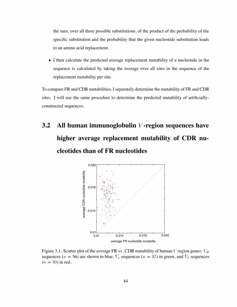
the sum, over all three possible substitutions, of the product of the probability of the

specific substitution and the probability that the given nucleotide substitution leads

to an amino acid replacement.

I then calculate the predicted average replacement mutability of a nucleotide in the

sequence is calculated by taking the average over all sites in the sequence of the

replacement mutability per site.

To compare FR and CDR mutabilities, I separately determine the mutability of FR and CDR

sites. I will use the same procedure to determine the predicted mutability of artificially-

constructed sequences.

3.2 All human immunoglobulin -region sequences have

higher average replacement mutability of CDR nu-

cleotides than of FR nucleotides

average FR nucleotide mutability

aver

age

CD

R n

ucle

otid

e m

utab

ility

0.01

0.014

0.018

0.022

0.01 0.014 0.018 0.022

Figure 3.1: Scatter plot of the average FR vs. CDR mutability of human region genes:sequences ( ) are shown in blue, sequences ( ) in green, and sequences( ) in red.

44

I extracted the sets of human -gene sequences from IMGT, the international Im-

MunoGeneTics database (Giudicelli et al., 1997). In cases where multiple alleles were

given for a certain locus, I only considered the first one in the database. I used the CDR/FR

assignment given in the IGMT alignments. As we were only interested in the properties

of the germline genes, I restricted the analysis to FR1, FR2, FR3, and CDR1, CDR2 frag-

ments. CDR3 is not entirely encoded by germline genes, but contains some non-templated

nucleotides, and I therefore left it out of these calculations. As shown in Fig. 3.1, all hu-

man region sequences, heavy as well as light chains, have higher average replacement

mutability of CDR nucleotides than of FR nucleotides.

To investigate what compositional biases are responsible for the difference in FR/CDR

mutability, for each of the germline sequences I constructed a number of variant sets:

Sets of variants of identical nucleotide composition, codon composition, or amino acid se-

quence. For illustration, let us focus on one initial data set, the set of human sequences.

For each sequence in this set, the set of sequences with identical FR/CDR nucleotide com-

position can be obtained by permuting the nucleotides in FR and CDR, separately. I con-

structed such variants for each of the germline sequences. If the mutability of a

sequence is completely determined by the relative proportion of the nucleotides in the se-

quence, then we expect that, by permuting the position of the nucleotides in the sequence,

its mutability will not be affected. As I will show below, this is not the case. However,

for some sequences, the average FR mutability of the set of variants is already lower than

their average CDR mutability. Therefore the nucleotide composition does play a role in the

differential mutability of FRs and CDRs, although it does not completely explain it.

Similarly, I construct variants of a sequence that have the same codon frequencies

in FR and CDR, by permuting the codons, separately, in the two regions. Using this data

set I investigate whether the mutability of the sequence is completely determined by its

codon composition. If this is the case, the mutability of the germline sequence will not be

significantly different than the average over its set of variants. If, on the other hand, the

linkage of codons also plays a role, the germline sequence will have a significantly different

45

mutability than the average over its set of variants. Whether the codon composition is

sufficient to explain the CDR-FR mutability difference is also a matter of intense debate.

My study is the first one that appropriately addresses this question. This is again due to the

capability of constructing variants of the sequence whose mutability can be calculated.

Finally, to obtain variants of a sequence with the same translation, I first determined

the amino acid sequence encoded by the germline gene. I then generated new nucleotide

sequences encoding the same amino acid sequence as follows. For each amino acid, I

choose, with uniform probability, one of the codons that could encode it, and add it to the

nucleotide sequence. This process is repeated for all amino acids in the protein sequence.

For each of the germline sequences, I constructed a set of such variants, which I call

translationally-neutral (that is, variants with the same amino acid translation). I then used

this set to test whether the mutability of the sequence is optimized through codon bias.

Having these variant sets, I could proceed to analyze the mutability of FRs and

CDRs in individual region sequences.

3.3 Statistical analysis on the level of individual sequences

One of the problems that limits the power of analysis of gene sequences is the lack of ap-

propriate controls. For example, for a given immunoglobulin sequence we do not have a

set of variants with identical amino acid translation that we can expose to somatic hyper-

mutation to compare their relative propensity to undergo amino acid replacements. Thus,

previous studies on differential mutability of FR and CDR of immunoglobulin had to use

large sequence sets, and no information could be derived on the level of individual se-

quences. Such is the case with the serine codon sets segregation pointed out by Wagner

et al. (1995), and, more generally, with the segregation of more mutable codons in CDRs

(Kepler, 1997). Moreover, these studies were restricted to mutability of in-frame triplets,

and did not use all the mutational information that might be present in the database of non-

selected mutations. All these problems are circumvented in the approach that I introduced

46

above.

The information concerning one sequence may be visually represented in the follow-

ing way. Each variant sequence corresponds to a point in the plane of FR/CDR mutability.

By taking the minimum and maximum FR and CDR mutability achieved by the variant

sequences, one can isolate a rectangle in this plane. I divided this rectangle into 100 by

100 smaller rectangles, which I call bins. If one counts the number of variant sequences

falling into each of the bins, one obtains a two-dimensional histogram. By sectioning the

two-dimensional histogram at the level of 1, 10, and 100 sequences per bin, one obtains

the contour plots that are shown in the figures. The outmost contour line corresponds to

densities of 1 sequence per bin, and the innermost one to densities of 100 sequences per

bin.

The possibility of analyzing the mutability of individual sequences allowed me to

attempt a more detailed understanding of the selection pressures that operate on individual

genes. For example, take a light chain sequence, V A2, the predominant germline gene

used in the immune response to Haemophilus influenzae in humans (Insel and Varade,

1998). Its predicted average FR and CDR nucleotide mutabilities are 1.2%, and 1.57%,

respectively, thus a CDR nucleotide is expected to undergo a replacement mutations 1.3

times more often than a FR nucleotide. Fig. 3.2 shows a contour plot of the distribution of

three sets of variants of this sequence in the FR-CDR mutability space. The set of sequences

with similar FR/CDR nucleotide composition is represented in black, the set of sequences

with similar codon composition in blue, and the translationally invariant set in green. The

position of the observed germline sequence is represented by the red dot. Of all the artificial

data sets, the set with identical codon composition has a mean FR/CDR mutability that

is most similar to that of the germline sequence. This allows me to conclude that the

mutability pattern of the observed is best predicted by its codon composition. The

CDR mutability is slightly higher than one could predict from its nucleotide sequence, and

I find codon usage bias consistent with low FR and high CDR mutability. Insel and Varade

(1998) found a low number of mutations in the complementarity-determining regions of

47

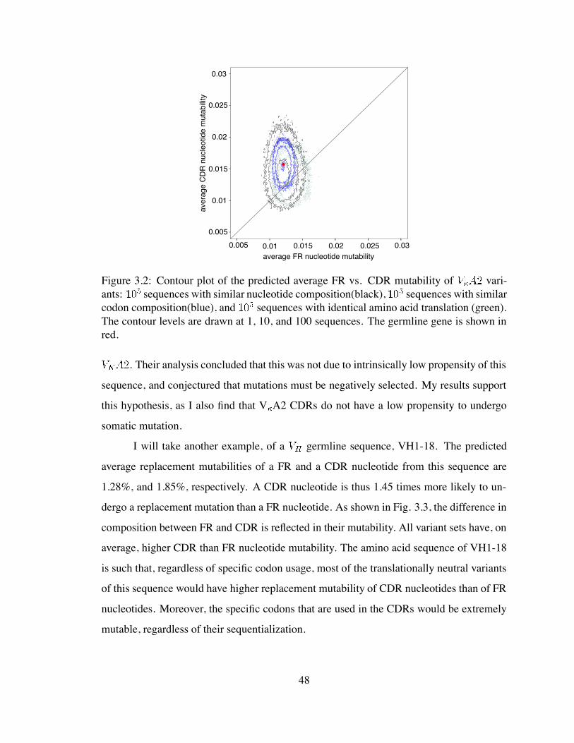
0.005 0.01 0.015 0.02 0.025 0.030.005

0.01

0.015

0.02

0.025

0.03

O

average FR nucleotide mutability

aver

age

CD

R n

ucle

otid

e m

utab

ility

Figure 3.2: Contour plot of the predicted average FR vs. CDR mutability of vari-ants: sequences with similar nucleotide composition(black), sequences with similarcodon composition(blue), and sequences with identical amino acid translation (green).The contour levels are drawn at 1, 10, and 100 sequences. The germline gene is shown inred.

. Their analysis concluded that this was not due to intrinsically low propensity of this

sequence, and conjectured that mutations must be negatively selected. My results support

this hypothesis, as I also find that V A2 CDRs do not have a low propensity to undergo

somatic mutation.

I will take another example, of a germline sequence, VH1-18. The predicted

average replacement mutabilities of a FR and a CDR nucleotide from this sequence are

1.28%, and 1.85%, respectively. A CDR nucleotide is thus 1.45 times more likely to un-

dergo a replacement mutation than a FR nucleotide. As shown in Fig. 3.3, the difference in

composition between FR and CDR is reflected in their mutability. All variant sets have, on

average, higher CDR than FR nucleotide mutability. The amino acid sequence of VH1-18

is such that, regardless of specific codon usage, most of the translationally neutral variants

of this sequence would have higher replacement mutability of CDR nucleotides than of FR

nucleotides. Moreover, the specific codons that are used in the CDRs would be extremely

mutable, regardless of their sequentialization.

48

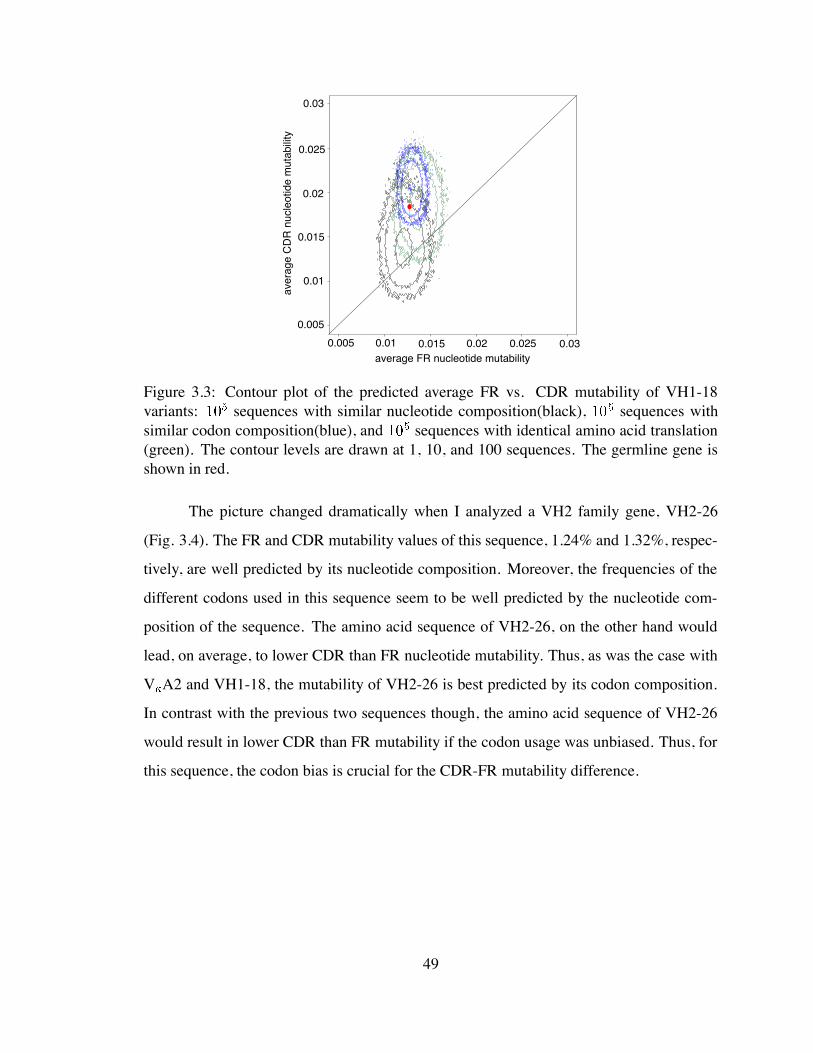
0.005 0.01 0.015 0.02 0.030.0250.005

0.01

0.015

0.02

0.03

0.025

average FR nucleotide mutability

aver

age

CD

R n

ucle

otid

e m

utab

ility

O

Figure 3.3: Contour plot of the predicted average FR vs. CDR mutability of VH1-18variants: sequences with similar nucleotide composition(black), sequences withsimilar codon composition(blue), and sequences with identical amino acid translation(green). The contour levels are drawn at 1, 10, and 100 sequences. The germline gene isshown in red.

The picture changed dramatically when I analyzed a VH2 family gene, VH2-26

(Fig. 3.4). The FR and CDR mutability values of this sequence, 1.24% and 1.32%, respec-

tively, are well predicted by its nucleotide composition. Moreover, the frequencies of the

different codons used in this sequence seem to be well predicted by the nucleotide com-

position of the sequence. The amino acid sequence of VH2-26, on the other hand would

lead, on average, to lower CDR than FR nucleotide mutability. Thus, as was the case with

V A2 and VH1-18, the mutability of VH2-26 is best predicted by its codon composition.

In contrast with the previous two sequences though, the amino acid sequence of VH2-26

would result in lower CDR than FR mutability if the codon usage was unbiased. Thus, for

this sequence, the codon bias is crucial for the CDR-FR mutability difference.

49

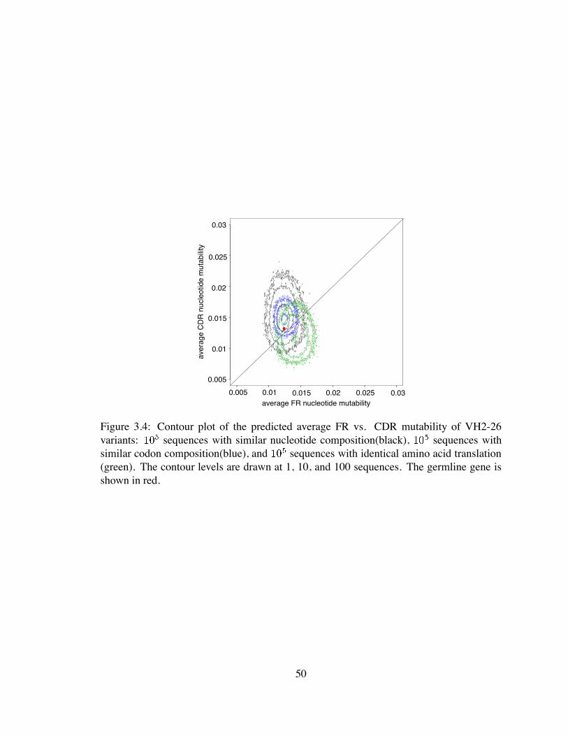
0.005 0.01 0.015 0.02 0.030.0250.005

0.01

0.015

0.02

0.03

0.025

average FR nucleotide mutability

aver

age

CD

R n

ucle

otid

e m

utab

ility

O

Figure 3.4: Contour plot of the predicted average FR vs. CDR mutability of VH2-26variants: sequences with similar nucleotide composition(black), sequences withsimilar codon composition(blue), and sequences with identical amino acid translation(green). The contour levels are drawn at 1, 10, and 100 sequences. The germline gene isshown in red.

50

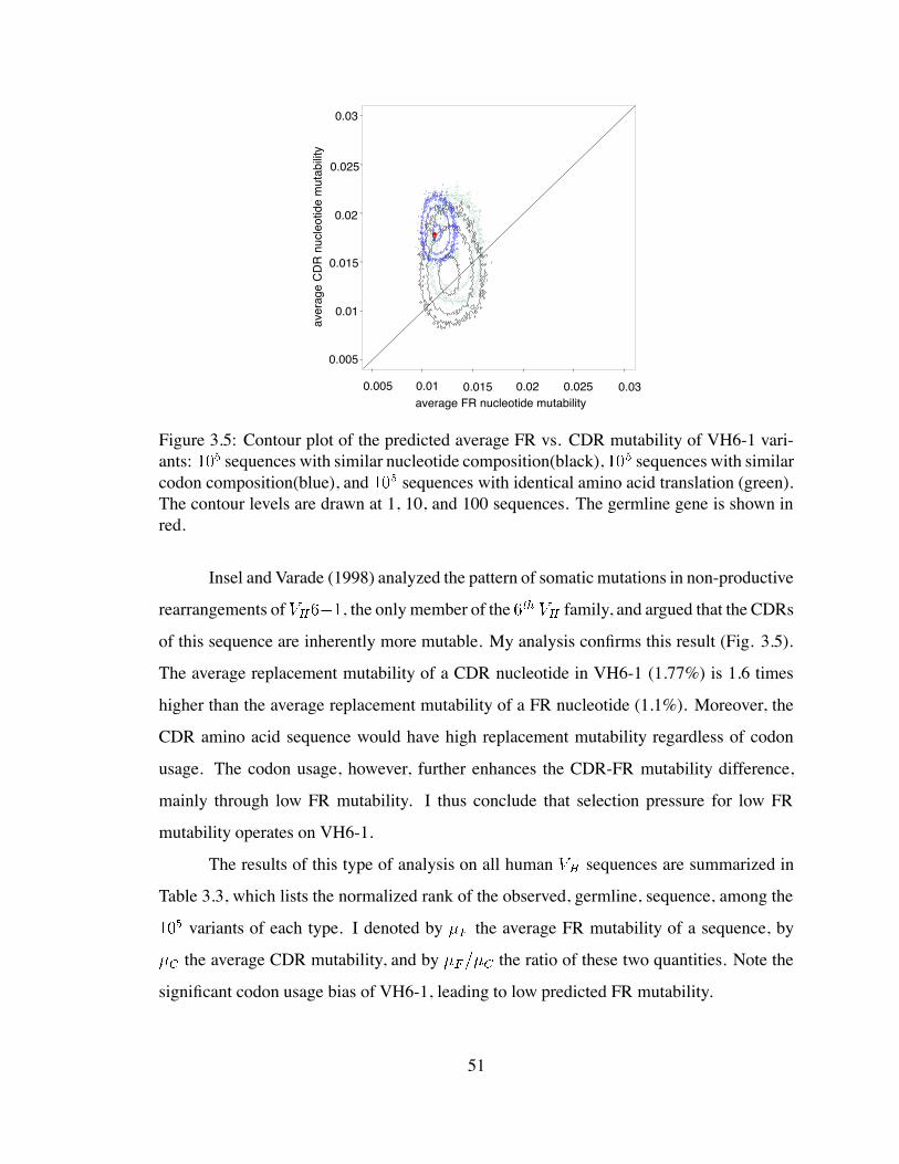
0.015

0.025

0.005

0.01

0.02

0.03

aver

age

CD

R n

ucle

otid

e m

utab

ility

0.015 0.02 0.030.025average FR nucleotide mutability

0.005 0.01

O

Figure 3.5: Contour plot of the predicted average FR vs. CDR mutability of VH6-1 vari-ants: sequences with similar nucleotide composition(black), sequences with similarcodon composition(blue), and sequences with identical amino acid translation (green).The contour levels are drawn at 1, 10, and 100 sequences. The germline gene is shown inred.

Insel and Varade (1998) analyzed the pattern of somatic mutations in non-productive

rearrangements of , the only member of the family, and argued that the CDRs

of this sequence are inherently more mutable. My analysis confirms this result (Fig. 3.5).

The average replacement mutability of a CDR nucleotide in VH6-1 (1.77%) is 1.6 times

higher than the average replacement mutability of a FR nucleotide (1.1%). Moreover, the

CDR amino acid sequence would have high replacement mutability regardless of codon

usage. The codon usage, however, further enhances the CDR-FR mutability difference,

mainly through low FR mutability. I thus conclude that selection pressure for low FR

mutability operates on VH6-1.

The results of this type of analysis on all human sequences are summarized in

Table 3.3, which lists the normalized rank of the observed, germline, sequence, among the

variants of each type. I denoted by the average FR mutability of a sequence, by

the average CDR mutability, and by the ratio of these two quantities. Note the

significant codon usage bias of VH6-1, leading to low predicted FR mutability.

51

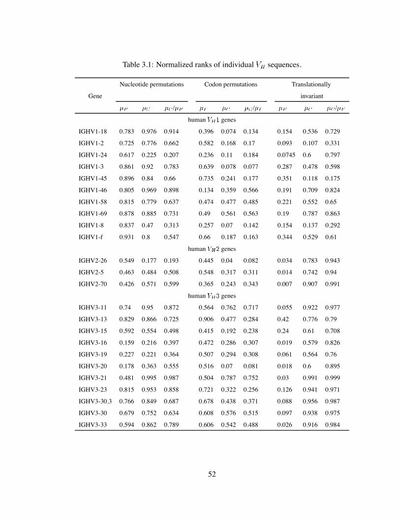
Table 3.1: Normalized ranks of individual sequences.

Nucleotide permutations Codon permutations Translationally

Gene invariant

/ / /

human genes

IGHV1-18 0.783 0.976 0.914 0.396 0.074 0.134 0.154 0.536 0.729

IGHV1-2 0.725 0.776 0.662 0.582 0.168 0.17 0.093 0.107 0.331

IGHV1-24 0.617 0.225 0.207 0.236 0.11 0.184 0.0745 0.6 0.797

IGHV1-3 0.861 0.92 0.783 0.639 0.078 0.077 0.287 0.478 0.598

IGHV1-45 0.896 0.84 0.66 0.735 0.241 0.177 0.351 0.118 0.175

IGHV1-46 0.805 0.969 0.898 0.134 0.359 0.566 0.191 0.709 0.824

IGHV1-58 0.815 0.779 0.637 0.474 0.477 0.485 0.221 0.552 0.65

IGHV1-69 0.878 0.885 0.731 0.49 0.561 0.563 0.19 0.787 0.863

IGHV1-8 0.837 0.47 0.313 0.257 0.07 0.142 0.154 0.137 0.292

IGHV1-f 0.931 0.8 0.547 0.66 0.187 0.163 0.344 0.529 0.61

human genes

IGHV2-26 0.549 0.177 0.193 0.445 0.04 0.082 0.034 0.783 0.943

IGHV2-5 0.463 0.484 0.508 0.548 0.317 0.311 0.014 0.742 0.94

IGHV2-70 0.426 0.571 0.599 0.365 0.243 0.343 0.007 0.907 0.991

human genes

IGHV3-11 0.74 0.95 0.872 0.564 0.762 0.717 0.055 0.922 0.977

IGHV3-13 0.829 0.866 0.725 0.906 0.477 0.284 0.42 0.776 0.79

IGHV3-15 0.592 0.554 0.498 0.415 0.192 0.238 0.24 0.61 0.708

IGHV3-16 0.159 0.216 0.397 0.472 0.286 0.307 0.019 0.579 0.826

IGHV3-19 0.227 0.221 0.364 0.507 0.294 0.308 0.061 0.564 0.76

IGHV3-20 0.178 0.363 0.555 0.516 0.07 0.081 0.018 0.6 0.895

IGHV3-21 0.481 0.995 0.987 0.504 0.787 0.752 0.03 0.991 0.999

IGHV3-23 0.815 0.953 0.858 0.721 0.322 0.256 0.126 0.941 0.971

IGHV3-30.3 0.766 0.849 0.687 0.678 0.438 0.371 0.088 0.956 0.987

IGHV3-30 0.679 0.752 0.634 0.608 0.576 0.515 0.097 0.938 0.975

IGHV3-33 0.594 0.862 0.789 0.606 0.542 0.488 0.026 0.916 0.984

52

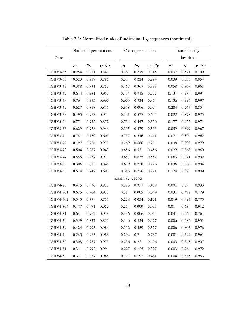
Table 3.1: Normalized ranks of individual sequences (continued).

Nucleotide permutations Codon permutations Translationally

Gene invariant

/ / /

IGHV3-35 0.254 0.211 0.342 0.367 0.279 0.345 0.037 0.571 0.799

IGHV3-38 0.523 0.819 0.785 0.37 0.224 0.294 0.039 0.856 0.954

IGHV3-43 0.388 0.731 0.753 0.467 0.367 0.393 0.058 0.867 0.961

IGHV3-47 0.614 0.981 0.952 0.434 0.715 0.727 0.131 0.986 0.994

IGHV3-48 0.76 0.995 0.966 0.663 0.924 0.864 0.136 0.995 0.997

IGHV3-49 0.627 0.888 0.815 0.678 0.096 0.09 0.204 0.767 0.854

IGHV3-53 0.495 0.983 0.97 0.341 0.527 0.605 0.022 0.878 0.975

IGHV3-64 0.77 0.955 0.872 0.734 0.447 0.356 0.177 0.955 0.971

IGHV3-66 0.629 0.978 0.944 0.395 0.479 0.533 0.059 0.899 0.967

IGHV3-7 0.741 0.759 0.603 0.737 0.516 0.411 0.071 0.89 0.962

IGHV3-72 0.197 0.966 0.977 0.269 0.686 0.77 0.038 0.893 0.979

IGHV3-73 0.504 0.967 0.943 0.656 0.53 0.456 0.022 0.863 0.969

IGHV3-74 0.555 0.957 0.92 0.657 0.635 0.552 0.063 0.971 0.992

IGHV3-9 0.306 0.813 0.848 0.639 0.258 0.226 0.036 0.966 0.994

IGHV3-d 0.574 0.742 0.692 0.383 0.226 0.291 0.124 0.82 0.909

human genes

IGHV4-28 0.415 0.936 0.923 0.293 0.357 0.489 0.001 0.59 0.933

IGHV4-301 0.625 0.964 0.923 0.35 0.005 0.049 0.031 0.472 0.779

IGHV4-302 0.545 0.79 0.751 0.228 0.034 0.121 0.019 0.493 0.775

IGHV4-304 0.477 0.971 0.952 0.254 0.009 0.095 0.01 0.63 0.912

IGHV4-31 0.64 0.962 0.918 0.336 0.006 0.05 0.041 0.466 0.76

IGHV4-34 0.359 0.837 0.851 0.146 0.224 0.427 0.006 0.686 0.931

IGHV4-39 0.424 0.993 0.984 0.312 0.459 0.577 0.006 0.806 0.976

IGHV4-4 0.245 0.985 0.986 0.294 0.7 0.767 0.001 0.644 0.961

IGHV4-59 0.308 0.977 0.975 0.236 0.22 0.406 0.003 0.543 0.907

IGHV4-61 0.31 0.992 0.99 0.227 0.125 0.327 0.003 0.76 0.972

IGHV4-b 0.31 0.987 0.985 0.127 0.192 0.461 0.004 0.685 0.953

53

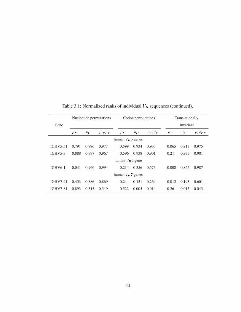
Table 3.1: Normalized ranks of individual sequences (continued).

Nucleotide permutations Codon permutations Translationally

Gene invariant

/ / /

human genes

IGHV5-51 0.791 0.996 0.977 0.599 0.934 0.903 0.065 0.917 0.975

IGHV5-a 0.888 0.997 0.967 0.596 0.938 0.901 0.21 0.975 0.981

human gene

IGHV6-1 0.041 0.966 0.994 0.214 0.356 0.573 0.008 0.855 0.987

human genes

IGHV7-41 0.453 0.886 0.869 0.24 0.131 0.264 0.012 0.193 0.601

IGHV7-81 0.893 0.515 0.319 0.522 0.005 0.014 0.26 0.015 0.043

54

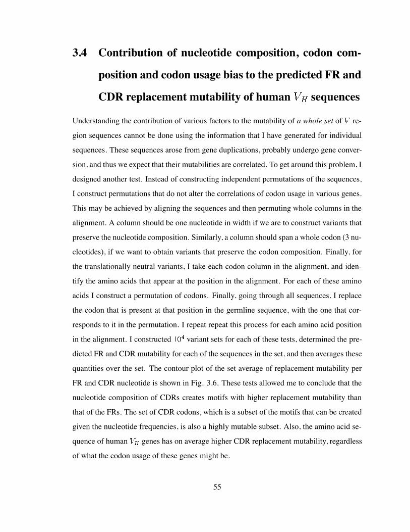
3.4 Contribution of nucleotide composition, codon com-

position and codon usage bias to the predicted FR and

CDR replacement mutability of human sequences

Understanding the contribution of various factors to the mutability of a whole set of re-

gion sequences cannot be done using the information that I have generated for individual

sequences. These sequences arose from gene duplications, probably undergo gene conver-

sion, and thus we expect that their mutabilities are correlated. To get around this problem, I

designed another test. Instead of constructing independent permutations of the sequences,

I construct permutations that do not alter the correlations of codon usage in various genes.

This may be achieved by aligning the sequences and then permuting whole columns in the

alignment. A column should be one nucleotide in width if we are to construct variants that

preserve the nucleotide composition. Similarly, a column should span a whole codon (3 nu-

cleotides), if we want to obtain variants that preserve the codon composition. Finally, for

the translationally neutral variants, I take each codon column in the alignment, and iden-

tify the amino acids that appear at the position in the alignment. For each of these amino

acids I construct a permutation of codons. Finally, going through all sequences, I replace

the codon that is present at that position in the germline sequence, with the one that cor-

responds to it in the permutation. I repeat repeat this process for each amino acid position

in the alignment. I constructed variant sets for each of these tests, determined the pre-

dicted FR and CDR mutability for each of the sequences in the set, and then averages these

quantities over the set. The contour plot of the set average of replacement mutability per

FR and CDR nucleotide is shown in Fig. 3.6. These tests allowed me to conclude that the

nucleotide composition of CDRs creates motifs with higher replacement mutability than

that of the FRs. The set of CDR codons, which is a subset of the motifs that can be created

given the nucleotide frequencies, is also a highly mutable subset. Also, the amino acid se-

quence of human genes has on average higher CDR replacement mutability, regardless

of what the codon usage of these genes might be.

55

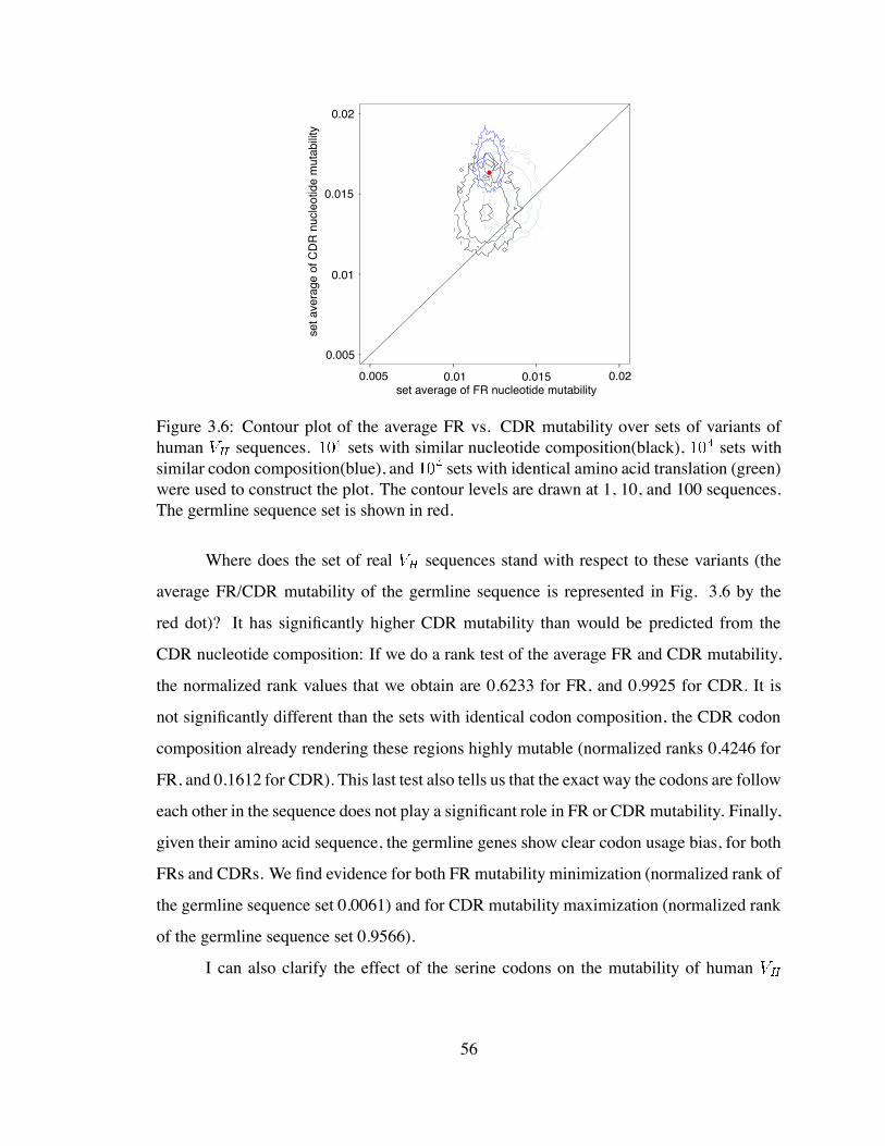
0.005 0.01 0.015 0.02

0.005

0.01

0.015

0.02

set average of FR nucleotide mutability

set a

vera

ge o

f CD

R n

ucle

otid

e m

utab

ility

Figure 3.6: Contour plot of the average FR vs. CDR mutability over sets of variants ofhuman sequences. sets with similar nucleotide composition(black), sets withsimilar codon composition(blue), and sets with identical amino acid translation (green)were used to construct the plot. The contour levels are drawn at 1, 10, and 100 sequences.The germline sequence set is shown in red.

Where does the set of real sequences stand with respect to these variants (the

average FR/CDR mutability of the germline sequence is represented in Fig. 3.6 by the

red dot)? It has significantly higher CDR mutability than would be predicted from the

CDR nucleotide composition: If we do a rank test of the average FR and CDR mutability,

the normalized rank values that we obtain are 0.6233 for FR, and 0.9925 for CDR. It is

not significantly different than the sets with identical codon composition, the CDR codon

composition already rendering these regions highly mutable (normalized ranks 0.4246 for

FR, and 0.1612 for CDR). This last test also tells us that the exact way the codons are follow

each other in the sequence does not play a significant role in FR or CDR mutability. Finally,

given their amino acid sequence, the germline genes show clear codon usage bias, for both

FRs and CDRs. We find evidence for both FR mutability minimization (normalized rank of

the germline sequence set 0.0061) and for CDR mutability maximization (normalized rank

of the germline sequence set 0.9566).

I can also clarify the effect of the serine codons on the mutability of human

56

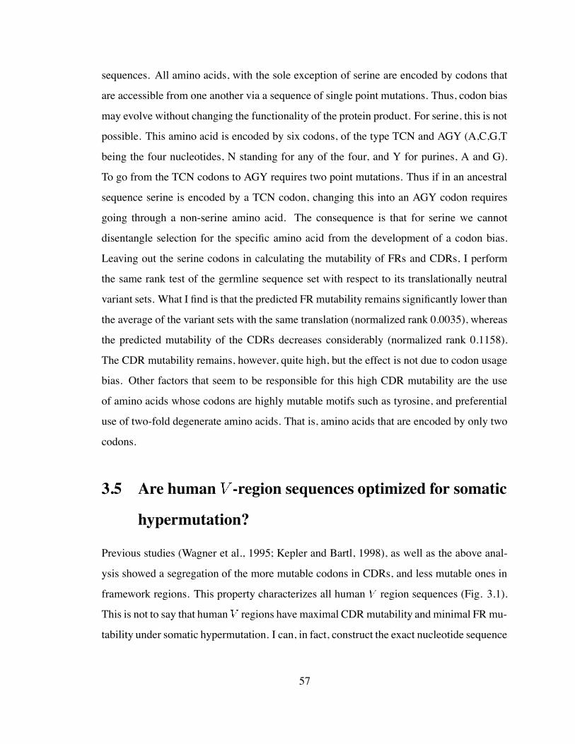
sequences. All amino acids, with the sole exception of serine are encoded by codons that

are accessible from one another via a sequence of single point mutations. Thus, codon bias

may evolve without changing the functionality of the protein product. For serine, this is not

possible. This amino acid is encoded by six codons, of the type TCN and AGY (A,C,G,T

being the four nucleotides, N standing for any of the four, and Y for purines, A and G).

To go from the TCN codons to AGY requires two point mutations. Thus if in an ancestral

sequence serine is encoded by a TCN codon, changing this into an AGY codon requires

going through a non-serine amino acid. The consequence is that for serine we cannot

disentangle selection for the specific amino acid from the development of a codon bias.

Leaving out the serine codons in calculating the mutability of FRs and CDRs, I perform

the same rank test of the germline sequence set with respect to its translationally neutral

variant sets. What I find is that the predicted FR mutability remains significantly lower than

the average of the variant sets with the same translation (normalized rank 0.0035), whereas

the predicted mutability of the CDRs decreases considerably (normalized rank 0.1158).

The CDR mutability remains, however, quite high, but the effect is not due to codon usage

bias. Other factors that seem to be responsible for this high CDR mutability are the use

of amino acids whose codons are highly mutable motifs such as tyrosine, and preferential

use of two-fold degenerate amino acids. That is, amino acids that are encoded by only two

codons.

3.5 Are human -region sequences optimized for somatic

hypermutation?

Previous studies (Wagner et al., 1995; Kepler and Bartl, 1998), as well as the above anal-

ysis showed a segregation of the more mutable codons in CDRs, and less mutable ones in

framework regions. This property characterizes all human region sequences (Fig. 3.1).

This is not to say that human regions have maximal CDR mutability and minimal FR mu-

tability under somatic hypermutation. I can, in fact, construct the exact nucleotide sequence

57

with this property for any of the region amino acid sequences. However, as I could not

assess the significance of the difference in mutability between the observed and the opti-

mal sequence, I designed instead another approach to look at the degree of optimality of

the germline sequence. Namely, I explore the neighborhood of the observed germline se-

quence in the space of silent mutants. These are the sequences to which evolution had most

immediate access. I shall describe the new experiment. I start with a germline sequence,

and generate variants of it, each of the variants differing from the germline sequence

by silent mutations. I calculate the predicted CDR and FR replacement mutabilities, and

their ratio, for each of the variants. I then determine the rank of the observed, germline,

sequence among its variants. Returning to the set of human sequences, among the 2

mutation neighbors, the proportion of sequences with higher CDR/FR mutability ratio than

the germline sequence varies between 38 and 52 percent. Among 10 mutation neighbors,

this proportion varies more widely, 25-65%. Among the 50 mutation neighbors, for some

germline sequence we find as few as 4% variants with higher ratio, whereas for some other

sequence, this proportion is 98.5%. Thus, the germline sequences are far from being op-

timal with respect to the differential mutability CDR/FR. It is a different issue whether

the selection pressure to select for a higher ratio is sufficiently high. For the 2 mutation

neighbors, the CDR/FR mutability ratio changes by fractions of a percent, and only for 10

mutation neighbors do we reach the level of percentages of the germline ratio. My conclu-

sion is therefore that, although all human sequences are characterized by lower FR than

CDR replacement mutability per nucleotide, the mutability of individual sequences is quite

far from optimal.

58

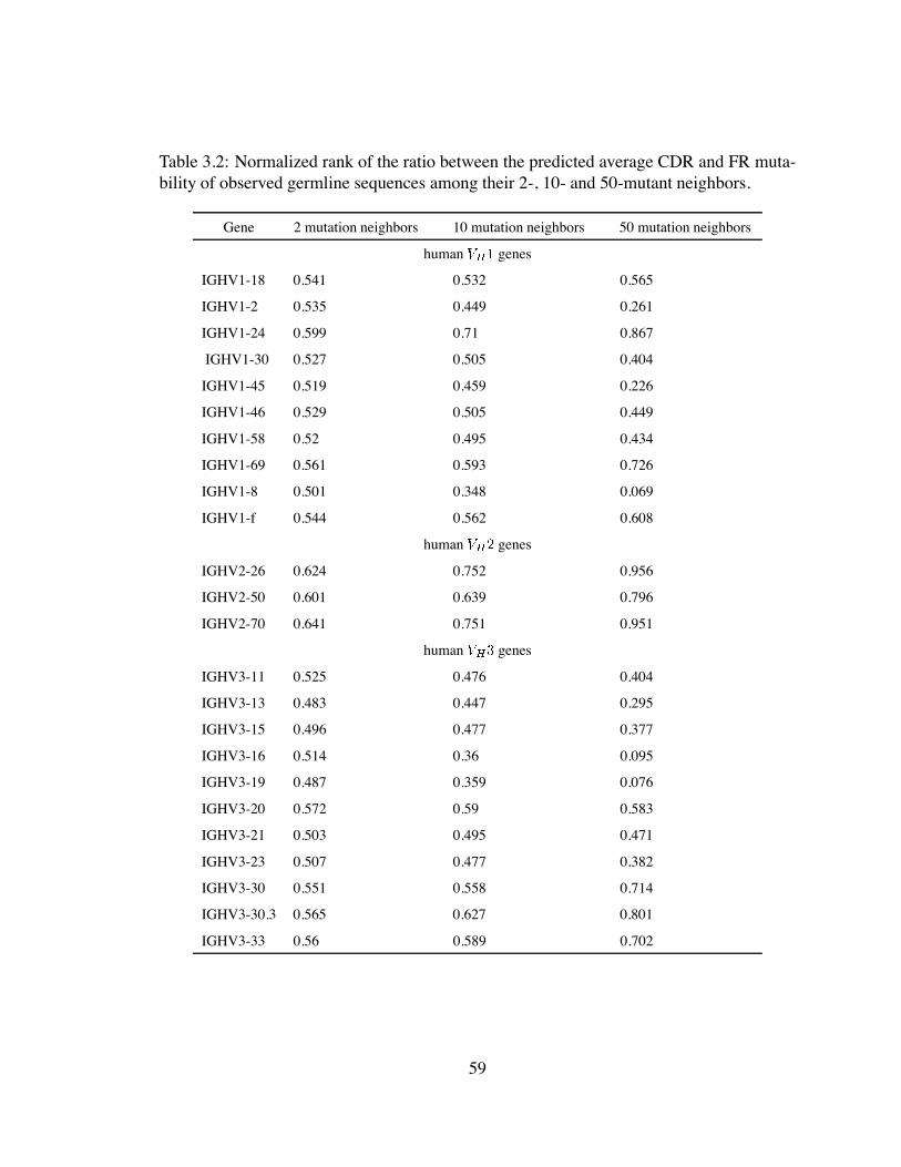
Table 3.2: Normalized rank of the ratio between the predicted average CDR and FR muta-bility of observed germline sequences among their 2-, 10- and 50-mutant neighbors.

Gene 2 mutation neighbors 10 mutation neighbors 50 mutation neighbors

human genes

IGHV1-18 0.541 0.532 0.565

IGHV1-2 0.535 0.449 0.261

IGHV1-24 0.599 0.71 0.867

IGHV1-30 0.527 0.505 0.404

IGHV1-45 0.519 0.459 0.226

IGHV1-46 0.529 0.505 0.449

IGHV1-58 0.52 0.495 0.434

IGHV1-69 0.561 0.593 0.726

IGHV1-8 0.501 0.348 0.069

IGHV1-f 0.544 0.562 0.608

human genes

IGHV2-26 0.624 0.752 0.956

IGHV2-50 0.601 0.639 0.796

IGHV2-70 0.641 0.751 0.951

human genes

IGHV3-11 0.525 0.476 0.404

IGHV3-13 0.483 0.447 0.295

IGHV3-15 0.496 0.477 0.377

IGHV3-16 0.514 0.36 0.095

IGHV3-19 0.487 0.359 0.076

IGHV3-20 0.572 0.59 0.583

IGHV3-21 0.503 0.495 0.471

IGHV3-23 0.507 0.477 0.382

IGHV3-30 0.551 0.558 0.714

IGHV3-30.3 0.565 0.627 0.801

IGHV3-33 0.56 0.589 0.702

59

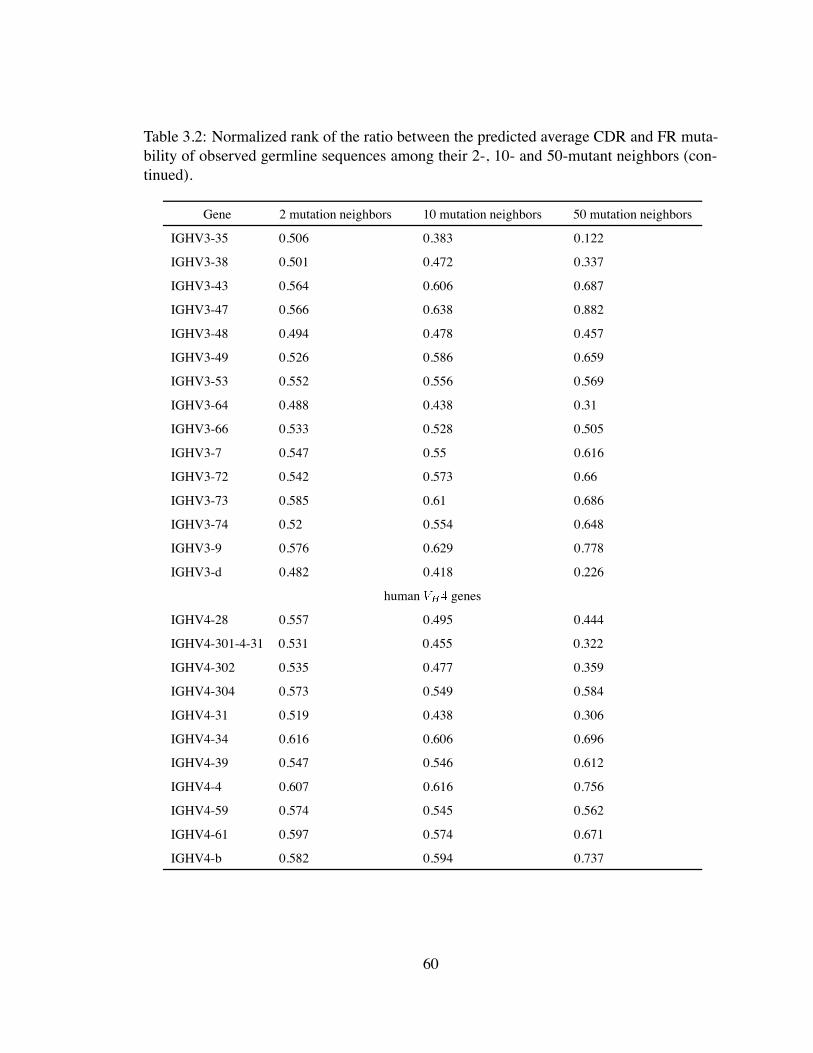
Table 3.2: Normalized rank of the ratio between the predicted average CDR and FR muta-bility of observed germline sequences among their 2-, 10- and 50-mutant neighbors (con-tinued).

Gene 2 mutation neighbors 10 mutation neighbors 50 mutation neighbors

IGHV3-35 0.506 0.383 0.122

IGHV3-38 0.501 0.472 0.337

IGHV3-43 0.564 0.606 0.687

IGHV3-47 0.566 0.638 0.882

IGHV3-48 0.494 0.478 0.457

IGHV3-49 0.526 0.586 0.659

IGHV3-53 0.552 0.556 0.569

IGHV3-64 0.488 0.438 0.31

IGHV3-66 0.533 0.528 0.505

IGHV3-7 0.547 0.55 0.616

IGHV3-72 0.542 0.573 0.66

IGHV3-73 0.585 0.61 0.686

IGHV3-74 0.52 0.554 0.648

IGHV3-9 0.576 0.629 0.778

IGHV3-d 0.482 0.418 0.226

human genes

IGHV4-28 0.557 0.495 0.444

IGHV4-301-4-31 0.531 0.455 0.322

IGHV4-302 0.535 0.477 0.359

IGHV4-304 0.573 0.549 0.584

IGHV4-31 0.519 0.438 0.306

IGHV4-34 0.616 0.606 0.696

IGHV4-39 0.547 0.546 0.612

IGHV4-4 0.607 0.616 0.756

IGHV4-59 0.574 0.545 0.562

IGHV4-61 0.597 0.574 0.671

IGHV4-b 0.582 0.594 0.737

60

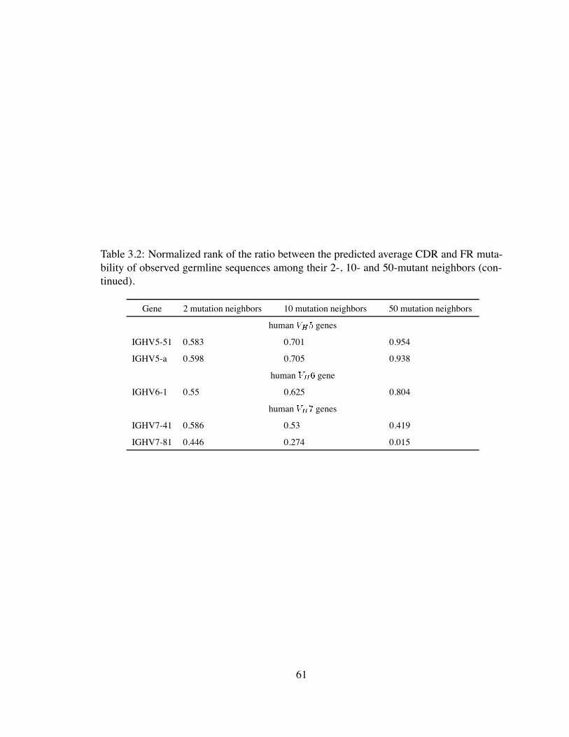
Table 3.2: Normalized rank of the ratio between the predicted average CDR and FR muta-bility of observed germline sequences among their 2-, 10- and 50-mutant neighbors (con-tinued).

Gene 2 mutation neighbors 10 mutation neighbors 50 mutation neighbors

human genes

IGHV5-51 0.583 0.701 0.954

IGHV5-a 0.598 0.705 0.938

human gene

IGHV6-1 0.55 0.625 0.804

human genes

IGHV7-41 0.586 0.53 0.419

IGHV7-81 0.446 0.274 0.015

61

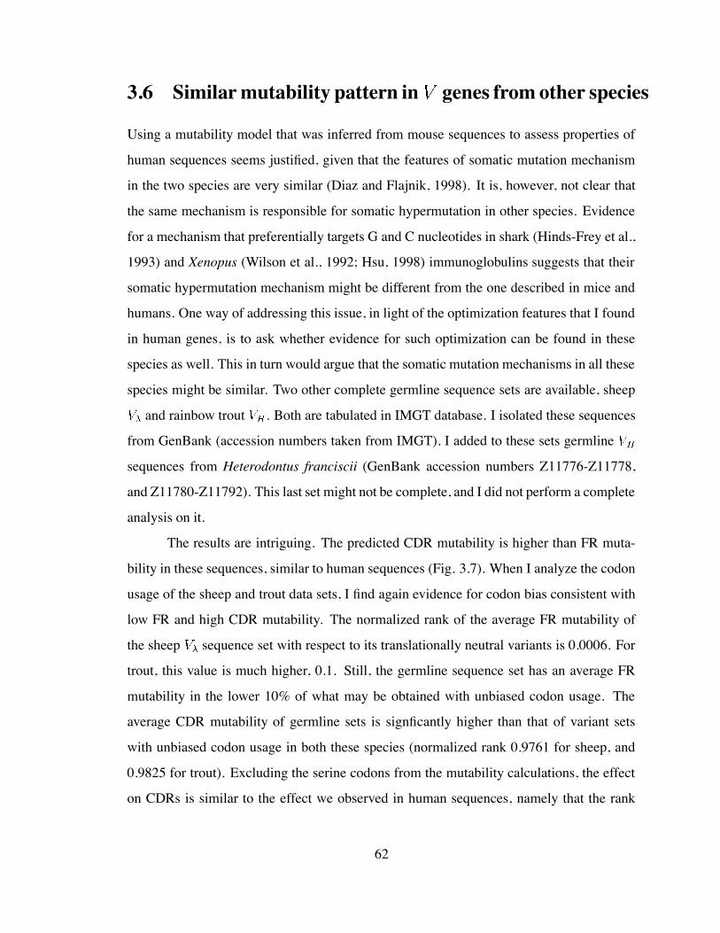
3.6 Similarmutability pattern in genes from other species

Using a mutability model that was inferred from mouse sequences to assess properties of

human sequences seems justified, given that the features of somatic mutation mechanism

in the two species are very similar (Diaz and Flajnik, 1998). It is, however, not clear that

the same mechanism is responsible for somatic hypermutation in other species. Evidence

for a mechanism that preferentially targets G and C nucleotides in shark (Hinds-Frey et al.,

1993) and Xenopus (Wilson et al., 1992; Hsu, 1998) immunoglobulins suggests that their

somatic hypermutation mechanism might be different from the one described in mice and

humans. One way of addressing this issue, in light of the optimization features that I found

in human genes, is to ask whether evidence for such optimization can be found in these

species as well. This in turn would argue that the somatic mutation mechanisms in all these

species might be similar. Two other complete germline sequence sets are available, sheep

and rainbow trout . Both are tabulated in IMGT database. I isolated these sequences

from GenBank (accession numbers taken from IMGT). I added to these sets germline

sequences from Heterodontus franciscii (GenBank accession numbers Z11776-Z11778,

and Z11780-Z11792). This last set might not be complete, and I did not perform a complete

analysis on it.

The results are intriguing. The predicted CDR mutability is higher than FR muta-

bility in these sequences, similar to human sequences (Fig. 3.7). When I analyze the codon

usage of the sheep and trout data sets, I find again evidence for codon bias consistent with

low FR and high CDR mutability. The normalized rank of the average FR mutability of

the sheep sequence set with respect to its translationally neutral variants is 0.0006. For

trout, this value is much higher, 0.1. Still, the germline sequence set has an average FR

mutability in the lower 10% of what may be obtained with unbiased codon usage. The

average CDR mutability of germline sets is signficantly higher than that of variant sets

with unbiased codon usage in both these species (normalized rank 0.9761 for sheep, and

0.9825 for trout). Excluding the serine codons from the mutability calculations, the effect

on CDRs is similar to the effect we observed in human sequences, namely that the rank

62

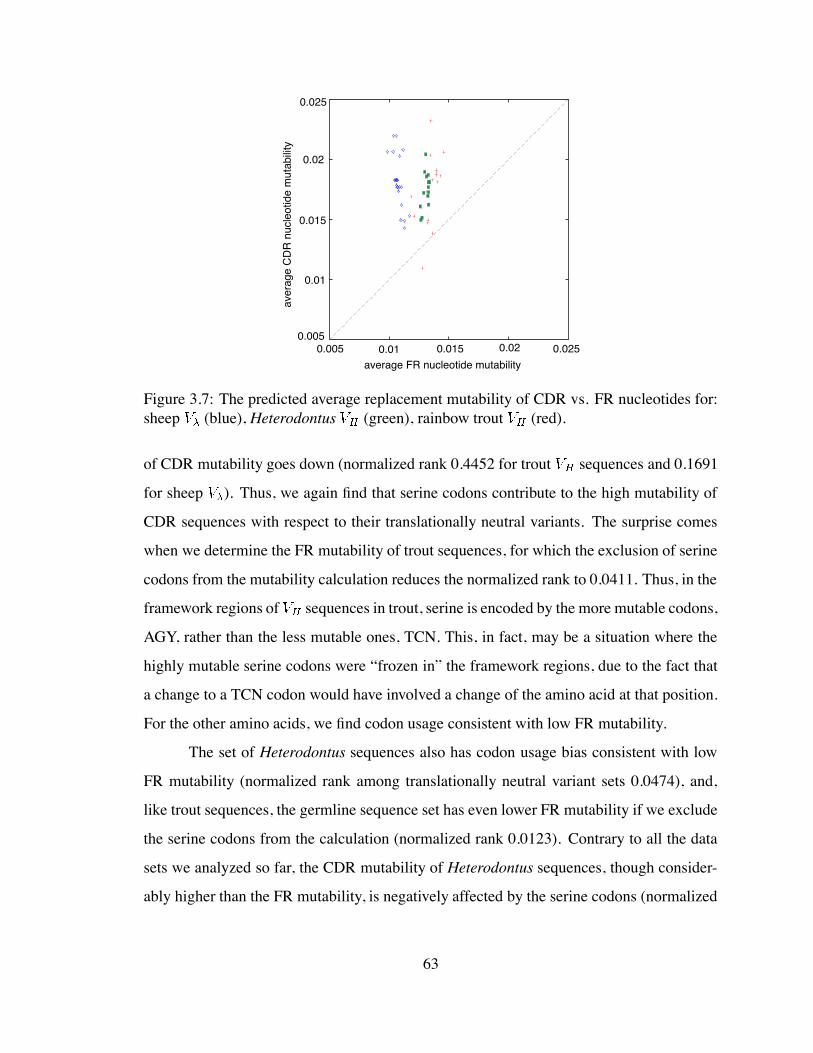
average FR nucleotide mutability

aver

age

CD

R n

ucle

otid

e m

utab

ility

0.0050.005

0.01

0.01

0.015

0.015

0.02

0.02

0.025

0.025

Figure 3.7: The predicted average replacement mutability of CDR vs. FR nucleotides for:sheep (blue), Heterodontus (green), rainbow trout (red).

of CDR mutability goes down (normalized rank 0.4452 for trout sequences and 0.1691

for sheep ). Thus, we again find that serine codons contribute to the high mutability of

CDR sequences with respect to their translationally neutral variants. The surprise comes

when we determine the FR mutability of trout sequences, for which the exclusion of serine

codons from the mutability calculation reduces the normalized rank to 0.0411. Thus, in the

framework regions of sequences in trout, serine is encoded by the more mutable codons,

AGY, rather than the less mutable ones, TCN. This, in fact, may be a situation where the

highly mutable serine codons were “frozen in” the framework regions, due to the fact that

a change to a TCN codon would have involved a change of the amino acid at that position.

For the other amino acids, we find codon usage consistent with low FR mutability.

The set of Heterodontus sequences also has codon usage bias consistent with low

FR mutability (normalized rank among translationally neutral variant sets 0.0474), and,

like trout sequences, the germline sequence set has even lower FR mutability if we exclude

the serine codons from the calculation (normalized rank 0.0123). Contrary to all the data

sets we analyzed so far, the CDR mutability of Heterodontus sequences, though consider-

ably higher than the FR mutability, is negatively affected by the serine codons (normalized

63

rank 0.6746 with serine codons, 0.8047 without). This is the consequence of serine being

encoded mostly by the low mutable codons TCN in Heterodontus CDRs.

I performed a similar test on Xenopus sequences, only to compare their mutability

pattern to those of theHeterodontus sequences. As I mentioned previously, there are claims

that a different mechanism is responsible for hypermutation in Xenopus and sharks as op-

posed to mammals (Wilson et al., 1992). For Xenopus, however, I used cDNA rather than

germline sequences. The cDNA is obtained by reverse transcribing the messenger RNA

of the cell into DNA. Thus these sequences may have already undergone somatic muta-

tion. I extracted the sequences from Kabat database, accession numbers KADBID004348,

KADBID004350-51, KADBID004353, KADBID004356-57, KADBID004359-61,

KADBID004365-66, KADBID004371, KADBID004376, KADBID004386. I translated

the nucleotide sequences, and then I aligned the amino acid sequences using ClustalW

(Higgins and Sharp, 1988) algorithm running on the European Bioinformatics Institute

server in Hinxton (Cambridge, UK), with the default parameters. This alignment was used

to infer the CDR/FR assignments.

I find that the high predicted CDR mutability of Xenopus sequences (normalized

rank 0.9909 among the variant sets with the same translation) is due to a large extent to the

usage of highly mutable serine codons, AGY. When I exclude the serine codons from the

mutability calculation, the CDR mutability decreases (normalized rank 0.6303 among the

translationally neutral variants). There is no evidence for codon usage bias consistent with

low FR mutability in these sequences. The normalized rank among the variant sets with

identical translation, and unbiased codon usage is 0.4227, or 0.6954, depending on whether

I do or do not include the serine codons in the mutability calculation.

The set of sheep sequences merits particular attention. In sheep, somatic hy-

permutation seems to be used as a diversification mechanism involved in generating the

primary repertoire (Reynaud et al., 1995), presumably without stringent antigen selection.

Testing the functionality of the immune receptors that are generated in this manner is prob-

ably delayed, allowing a number of mutations to be introduced in the gene. These are likely

64

to render the sequence non-functional. We expect that selection pressure for undergoing a

minimal number of FR mutations is operating in these sequences. I thus decided to analyze

these sequences individually, looking for evidence for codon usage bias that would render

the framework regions of these sequences resistant to replacement mutations. Indeed, I find

that the predicted replacement mutability of FR nucleotides is rendered extremely low by

the codon bias (Table 3.3).

Summarizing these results:

Higher predicted mutability of CDR than of FR nucleotides is a general feature in

all germline sequence sets used in this study. In addition, I tested that this property

holds for two germline sequences of nurse shark antigen receptor (Roux et al., 1998),

as well as by cDNA sequences from Xenopus.

With the exception of Xenopus, all data sets that I analyzed show evidence for codon

bias consistent with low FR mutability. For trout and Heterodontus sequences,

this bias is stronger if I exclude the serine codons from the mutability calculation.

This indicates that the highly mutable serine codons, AGY, are used in the FR regions

in these species at high frequencies relative to the low mutable ones, TCN. This

seems an interesting situation, in which the highly mutable serine codons have been

“frozen into” the sequence during evolution.

The predicted CDR mutability is invariably high, although different factors con-

tribute to it in different species.

Contrary to the current view (Diaz and Flajnik, 1998), the mutability pattern of

Heterodontus sequences resembles that of mammalian, rather than Xenopus se-

quences.

The finding that codon usage bias consistent with low FR and high CDR mutabil-

ity is present in all but one of the species that I studied, supports the hypothesis that the

components of the somatic hypermutation mechanisms are similar in these species. The

65

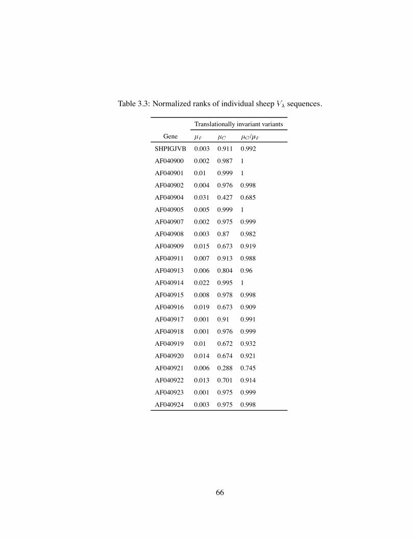
Table 3.3: Normalized ranks of individual sheep sequences.

Translationally invariant variants

Gene /

SHPIGJVB 0.003 0.911 0.992

AF040900 0.002 0.987 1

AF040901 0.01 0.999 1

AF040902 0.004 0.976 0.998

AF040904 0.031 0.427 0.685

AF040905 0.005 0.999 1

AF040907 0.002 0.975 0.999

AF040908 0.003 0.87 0.982

AF040909 0.015 0.673 0.919

AF040911 0.007 0.913 0.988

AF040913 0.006 0.804 0.96

AF040914 0.022 0.995 1

AF040915 0.008 0.978 0.998

AF040916 0.019 0.673 0.909

AF040917 0.001 0.91 0.991

AF040918 0.001 0.976 0.999

AF040919 0.01 0.672 0.932

AF040920 0.014 0.674 0.921

AF040921 0.006 0.288 0.745

AF040922 0.013 0.701 0.914

AF040923 0.001 0.975 0.999

AF040924 0.003 0.975 0.998

66

selection pressures that operate in these different species would be difficult to estimate. It

is generally believed that selection is weaker in B cells of Xenopus (Wilson et al., 1992;

Hsu, 1998), and it is possible that the different mutability pattern in this species comes

from lower selection pressure on FR mutability. After all, the CDR mutability is already

higher than FR mutability in Xenopus, similar to all the other species. We cannot, however,

exclude the possibility that different mechanisms are responsible for somatic mutation in

Xenopus, as opposed to mammalian species.

3.7 Higher predicted replacement mutability of T cell re-

ceptor CDRs than T cell receptor FRs

Zheng et al. (1994) isolated individual germinal centers T cells and sequenced their immune

receptor genes. Surprisingly, they found a number of mutations in these genes, raising the

intriguing possibility that T cell receptors also undergo somatic hypermutation. The muta-

tions that were found in these T cell receptors seemed to bear the mark of somatic hyper-

mutation. That is, only germinal center T cells, already recruited in the immune response

were affected, mutations were mostly found in the CDRs and they were concentrated in

the hot spots described for B cell receptor hypermutation. This finding challenges one of

the basic paradigms of self-nonself discrimination. It is generally believed that during their

development in the thymus, T cells that bind any antigen with sufficiently high affinity are

destined to die. On the contrary, when T cells bind antigens with high affinity outside of

the thymus, they start replicating and performing their effector functions. T cell receptor

mutation in the germinal centers may then turn a benign T cell into an auto-reactive one.

Evidently, this finding raised a lot of controversy.

Kepler and Bartl (1998), looking for the presence of mutable motifs in T cell recep-

tors CDRs concluded that some of the T-cell receptor chains resemble immunoglobulins in

their mutability pattern, but a consistent trend could not be identified. Human TCR did

not show the immunoglobulin mutability pattern, whereas murine did, although only

67

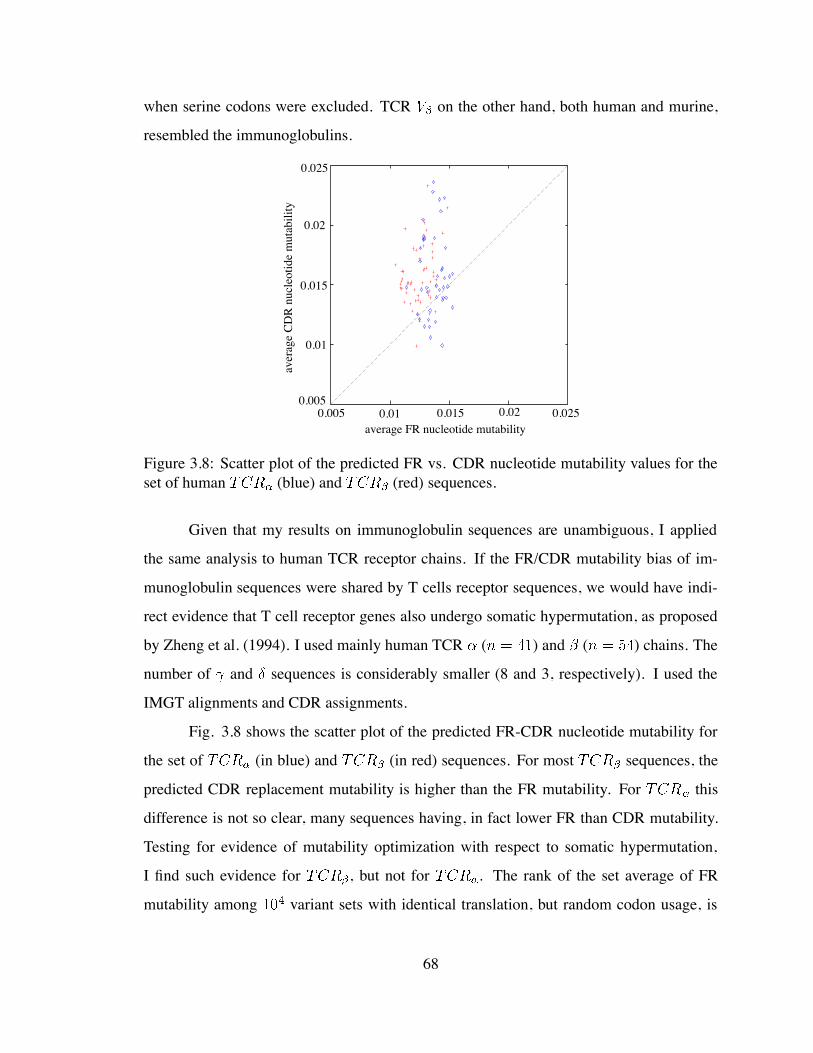
when serine codons were excluded. TCR on the other hand, both human and murine,

resembled the immunoglobulins.

average FR nucleotide mutability0.005 0.01 0.015 0.02 0.025

0.005

0.01

0.015

0.02

0.025

aver

age

CDR

nucl

eotid

e m

utab

ility

Figure 3.8: Scatter plot of the predicted FR vs. CDR nucleotide mutability values for theset of human (blue) and (red) sequences.

Given that my results on immunoglobulin sequences are unambiguous, I applied

the same analysis to human TCR receptor chains. If the FR/CDR mutability bias of im-

munoglobulin sequences were shared by T cells receptor sequences, we would have indi-

rect evidence that T cell receptor genes also undergo somatic hypermutation, as proposed

by Zheng et al. (1994). I used mainly human TCR ( ) and ( ) chains. The

number of and sequences is considerably smaller (8 and 3, respectively). I used the

IMGT alignments and CDR assignments.

Fig. 3.8 shows the scatter plot of the predicted FR-CDR nucleotide mutability for

the set of (in blue) and (in red) sequences. For most sequences, the

predicted CDR replacement mutability is higher than the FR mutability. For this

difference is not so clear, many sequences having, in fact lower FR than CDR mutability.

Testing for evidence of mutability optimization with respect to somatic hypermutation,

I find such evidence for , but not for . The rank of the set average of FR

mutability among variant sets with identical translation, but random codon usage, is

68

0.0103 in the case of , and 0.3524 in the case of . CDR mutability ranks

0.9581 in the case of , and 0.3941 in the case of .

These results allow a number of interpretations. They could indicate that somatic

hypermutation currently affects T cell receptors, as suggested by Zheng et al. (1994). They

could also indicate that the hypermutation mechanism does not operate in these genes cur-

rently, but it affected the ancestral receptor from which immunoglobulins and T cell recep-

tors diverged. This feature would then have been preserved in immunoglobulin chains, but

lost in T cells, whose sequence drifted away from the one that supported somatic muta-

tion. The mutability pattern of immunoglobulins in other species also argues for somatic

mutation being discovered early in phylogeny. This has also been suggested by M.Flajnik

(personal communication, 1998). Finally, this result could indicate that the somatic hy-

permutation mechanism adapted to the codon bias of immunoglobulin genes. This codon

bias could be shared by some of the T cell receptor genes, by virtue of the genealogical

relationship between T cell and B cell receptors.

69

Chapter 4

Non-immunoglobulin genes would have

low mutability under somatic

hypermutation

As mentioned in the previous chapter, the nature of the somatic hypermutation mechanism

is not known. Attempts to show the involvement of mismatch repair mechanisms, that

is, the mechanisms that recognize and repair base pairs other than Watson-Crick A-T and

G-C, in this process led to ambiguous results (Cascalho et al., 1998; Winter et al., 1998;

Frey et al., 1998; Kelsoe, 1998). There is a sense though, that an error-prone polymerase

might be involved (Phung et al., 1998), or, more generally, that normally expressed gene

products have been recruited in the somatic hypermutation mechanism (Kelsoe, 1998).

In order to test the involvement of these general mutation/repair mechanisms in somatic

hypermutation, I stated the following hypothesis. If both:

more general mutation/repair mechanisms have been recruited for somatic hypermu-

tation, and

genes tend to evolve mutational robustness (Wagner, 1999, and E. van Nimwegen,

personal communication, 1999)

70

then I might be able to detect optimization features with respect to the somatic mutator in

non-immunoglobulin genes. Concretely, in light of my previous results, I would expect to

detect codon usage bias consistent with low mutability in non-immunoglobulin genes.

In the following sections I will show that such codon bias is indeed present in a

large fraction of the non-immunoglobulin sequences that I analyzed. It is not a random

codon bias that the somatic hypermutation mechanism happens to reveal; none of 100 other

codon biases that I analyzed produced as many sequences with very low mutability as the

codon bias present in the genome. If non-immunoglobulin genes were to undergo somatic

hypermutation, they would generally have a low propensity to mutate. A striking finding is

that their mutability would be correlated with the A and T nucleotide composition, and that

this correlation is not entirely observable in the mutability model that I used. This finding

may be a small step towards revealing the nature of the somatic hypermutation mechanism,

that virtually every laboratory that studies somatic mutation is trying to identify.

4.1 In non-immunoglobulin genes, predicted mutability is

correlated with A/T content

The main mechanisms that have so far been invoked to explain codon usage bias within

genomes are concerned with either transcriptional efficiency (Ikemura, 1981, 1985), or with

the stability of the nucleic acids, or of the encoded proteins (Bernardi and Bernardi, 1986).

In a study of Bernardi and Bernardi (1986), it was shown that codon usage in genomes

is determined by compositional constraints. That is, it was shown that the G/C content at

the third, degenerate, position of the codons in a gene is correlated with the overall G/C

content in the genome compartment where the gene resides. These in turn have to do with

the stability of both nucleic acids and proteins, which depend on environmental pressures.

Warm-blooded vertebrates have higher G/C content in their genes, which correlates with the

stability of mRNA molecules. The amino acid replacements resulting from increasing G/C

content have been shown to also lead to more thermodynamically stable proteins (Argos

71

et al., 1979; Zuber, 1981).

With this mechanism in mind, I performed the following test. I used the empirical

mutability model described in chapter 3 to calculate an average mutability per nucleotide

for a number of non-immunoglobulin genes. I also determined the A/T content of the

genes. Surprisingly, mutability is correlated with the A/T-content of the genes. Thus, ad-

justments in the nucleotide composition of non-immunoglobulin genes, that are associated

with higher stability of the DNA and mRNA, seem to correlate with low apparent mutabil-

ity under somatic hypermutation. This result raises the interesting hypothesis that somatic

hypermutation may involve mispairing of nucleotides during DNA synthesis (this event

being more probable for A and T nucleotides), the resulting lesion failing to be repaired.

Alternatively, it may reflect a bias in the repair mechanism.

For this study, I extracted a set of 140 human non-immunoglobulin genes from

GenBank (Appendix A). I performed a pairwise alignment of all amino acid sequences, to

ensure that no close relation existed between any two sequences. That is because I want

to assess the significance of the biases that are found in random genes in the genome, and

this biases should not be due to the genealogical relationship between sequences. I first

determined the total mutability (both silent and replacement) per nucleotide for all these

sequences. As shown in Fig. 4.1, the mutability of a sequence is anti-correlated with the

G/C content of the sequence. The correlation becomes even more significant when I calcu-

late the replacement mutability rather than total mutability of a nucleotide in each sequence

(Fig. 4.2). This correlation can be predicted qualitatively from the mutability matrix that we

used. The A/T content of individual triplets (which takes discrete values: 0, 1/3, 2/3, and 1)

is already predictive of mutability. However, the correlation is considerably stronger in real

genes. Table 4.1 summarizes the results of the correlation test that I performed on triplet

mutability, and total and replacement mutability per nucleotide for non-immunoglobulin

sequences.

This is precisely what previous studies of mutations that occur spontaneous in the

genome evolution reported Bernardi and Bernardi (1986); Wolfe et al. (1989); Li (1997). It

72

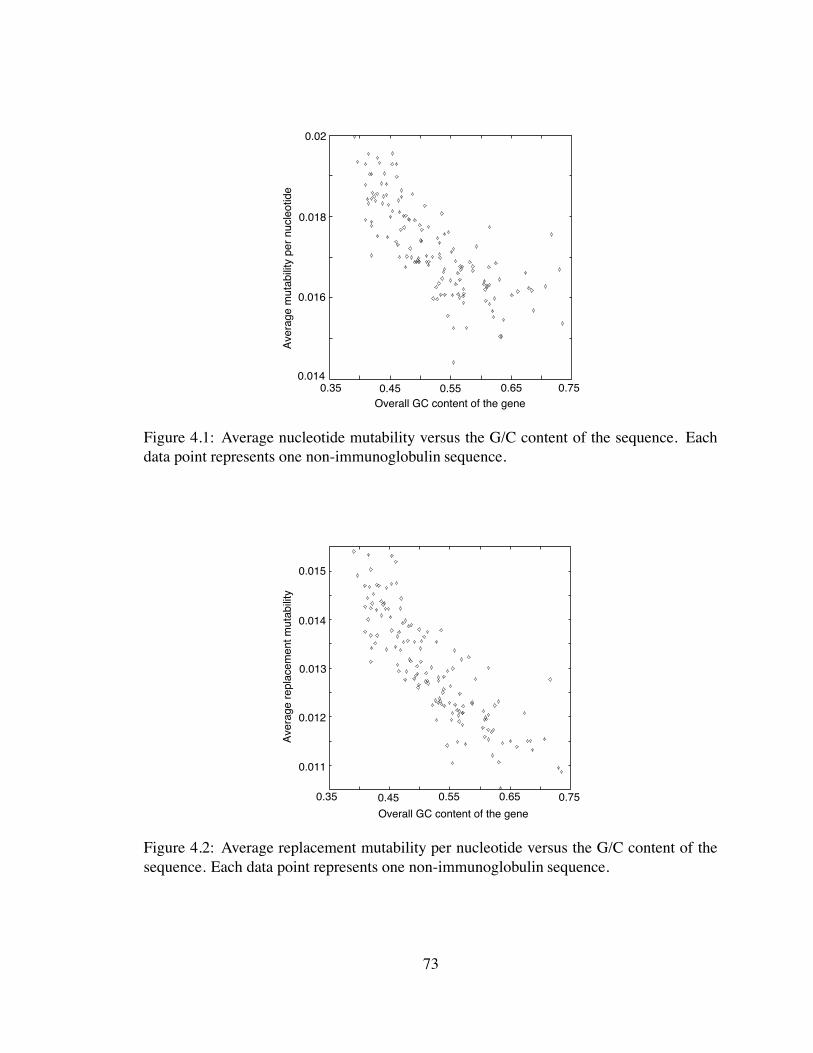
0.014

0.016

0.018

0.02

0.35 0.45 0.55 0.65 0.75Overall GC content of the gene

Aver

age

mut

abilit

y pe

r nuc

leot

ide

Figure 4.1: Average nucleotide mutability versus the G/C content of the sequence. Eachdata point represents one non-immunoglobulin sequence.

0.011

0.012

0.013

0.014

0.015

0.35 0.45 0.55 0.65 0.75Overall GC content of the gene

Aver

age

repl

acem

ent m

utab

ility

Figure 4.2: Average replacement mutability per nucleotide versus the G/C content of thesequence. Each data point represents one non-immunoglobulin sequence.

73

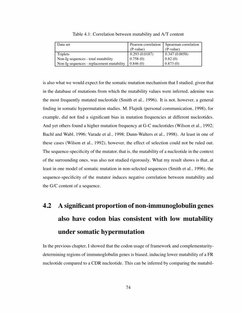
Table 4.1: Correlation between mutability and A/T content

Data set Pearson correlation Spearman correlation(P-value) (P-value)

Triplets 0.293 (0.0187) 0.347 (0.0058)Non-Ig sequences - total mutability 0.758 (0) 0.82 (0)Non-Ig sequences - replacement mutability 0.846 (0) 0.873 (0)

is also what we would expect for the somatic mutation mechanism that I studied, given that

in the database of mutations from which the mutability values were inferred, adenine was

the most frequently mutated nucleotide (Smith et al., 1996). It is not, however, a general

finding in somatic hypermutation studies. M. Flajnik (personal communication, 1998), for

example, did not find a significant bias in mutation frequencies at different nucleotides.

And yet others found a higher mutation frequency at G-C nucleotides (Wilson et al., 1992;

Bachl and Wabl, 1996; Varade et al., 1998; Dunn-Walters et al., 1998). At least in one of

these cases (Wilson et al., 1992), however, the effect of selection could not be ruled out.

The sequence-specificity of the mutator, that is, the mutability of a nucleotide in the context

of the surrounding ones, was also not studied rigorously. What my result shows is that, at

least in one model of somatic mutation in non-selected sequences (Smith et al., 1996), the

sequence-specificity of the mutator induces negative correlation between mutability and

the G/C content of a sequence.

4.2 A significant proportion of non-immunoglobulin genes

also have codon bias consistent with low mutability

under somatic hypermutation

In the previous chapter, I showed that the codon usage of framework and complementarity-

determining regions of immunoglobulin genes is biased, inducing lower mutability of a FR

nucleotide compared to a CDR nucleotide. This can be inferred by comparing the mutabil-

74

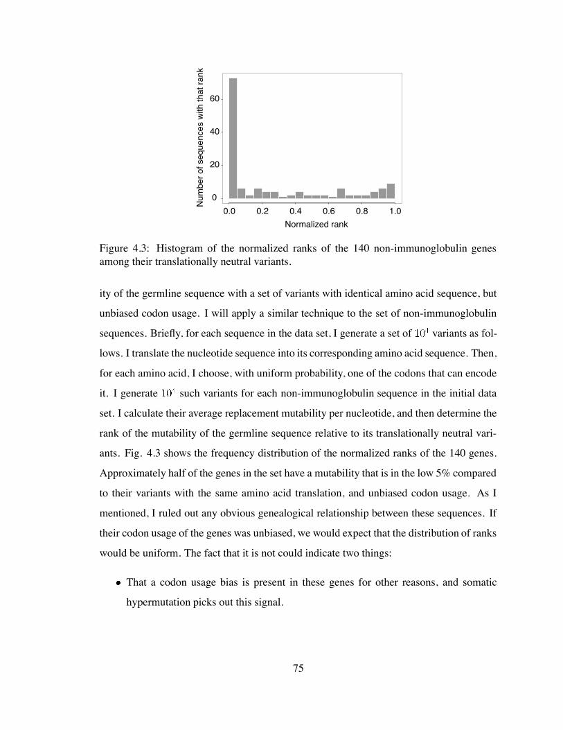
0.0 0.2 0.4 0.6 0.8 1.00

20

40

60

Normalized rank

Num

ber o

f seq

uenc

es w

ith th

at ra

nk

Figure 4.3: Histogram of the normalized ranks of the 140 non-immunoglobulin genesamong their translationally neutral variants.

ity of the germline sequence with a set of variants with identical amino acid sequence, but

unbiased codon usage. I will apply a similar technique to the set of non-immunoglobulin

sequences. Briefly, for each sequence in the data set, I generate a set of variants as fol-

lows. I translate the nucleotide sequence into its corresponding amino acid sequence. Then,

for each amino acid, I choose, with uniform probability, one of the codons that can encode

it. I generate such variants for each non-immunoglobulin sequence in the initial data

set. I calculate their average replacement mutability per nucleotide, and then determine the

rank of the mutability of the germline sequence relative to its translationally neutral vari-

ants. Fig. 4.3 shows the frequency distribution of the normalized ranks of the 140 genes.

Approximately half of the genes in the set have a mutability that is in the low 5% compared

to their variants with the same amino acid translation, and unbiased codon usage. As I

mentioned, I ruled out any obvious genealogical relationship between these sequences. If

their codon usage of the genes was unbiased, we would expect that the distribution of ranks

would be uniform. The fact that it is not could indicate two things:

That a codon usage bias is present in these genes for other reasons, and somatic

hypermutation picks out this signal.

75

That these genes share a codon usage bias consistent with low mutability because

the somatic hypermutation mechanism borrows components from a mechanism that

operates with a much larger scope in the genome than immunoglobulin genes.

I attempted to decide between these alternatives using the following test. Let us

generate a different codon usage bias. Let be the set of codons, where denotes the

amino acid that the codon is specifying. Let be a random permutation of the codons

encoding amino acid . Then to construct a sequence under this new codon usage bias, I

replace each codon in the sequence by . The set , with constitutes

the new codon usage bias. For each codon bias thus constructed, I re-generate the set of 140

gene sequences, and calculate their replacement mutability under somatic mutation. Due

to computational constraints, I only generated 100 different permutations of the codons.

As I showed previously (Fig. 4.3), 73 of the 140 non-immunoglobulin sequences

that I studied have codon usage that places them in the lowest 5% in mutability among

their translationally invariant variants. In fact, 66 of the 140 sequences are in the lowest

1% among their neutral variants. I generate similar sets of translationally neutral variants

for each sequence under each codon usage bias. I then determine how many of these codon

usage biases give us as many significantly low mutable sequences. It turns out that if I

set the significance level at the normalized rank of 1% among the neutral variants, none of

the codon usage biases can produce as many low mutable sequences as the original codons

usage bias.

This result allows me to conclude that it is not a random codon usage bias that the

somatic hypermutation mechanism would pick out of these sequences. It is specifically

the codon bias present in the set of germline genes that I used for this study. Thus, there

is a significant correlation between the sequence specificity of the somatic hypermutation

mechanism and the codon bias present in human genes. This may be due to:

Somatic mutation being derived from a more general mutation mechanism that oper-

ates on the level of the whole genome.

76

Somatic mutation having evolved to exploit a codon usage bias already present in the

genome.

At the moment, I cannot decide between these two alternatives. On a simplicity argu-

ment, I tend to favor the first hypothesis. If the somatic mutator is derived from a more

general-purpose mutation mechanism, we would expect that gene sequences, including im-

munoglobulin gene sequences, already had low mutability at the time when the mutator

appeared. Only codon bias in CDRs would need to be evolved to arrive at the current mu-

tability data. On the other hand, if a whole new mutation mechanism was evolved, it had to

first adjust to the codon usage bias of the genome, and then the CDRs evolved a different

codon usage. Whether the simplest path was indeed taken in the evolution of the immune

system remains to be seen.

77

Chapter 5

Mutants must be generated and selected

in a step-wise fashion during the

germinal center reaction

5.1 Affinity maturation during the germinal center reac-

tion

Somatic hypermutation seems to take place only during on-going immune responses, in the

germinal center (GC) microenvironment. Germinal centers are specific anatomical sites

in lymph nodes, spleen and other secondary lymphoid organs. They have an ephemeral

existence, arising during the first week of an immune response, and lasting for approxi-

mately four weeks. They are believed to support the process of affinity maturation through

somatic hypermutation (Weigert et al., 1970; Bernard et al., 1978) and affinity-based selec-

tion (Berek et al., 1991; Jacob and Kelsoe, 1992; Nossal, 1992) of antigen-specific B cells.

The term affinity maturation is simply used to describe the observation that the affinity of

the antibodies that bind a given antigen at the end of the immune response is higher than

the affinity of the antibodies that first reacted to this antigen. Thus the affinity ”matures”

78

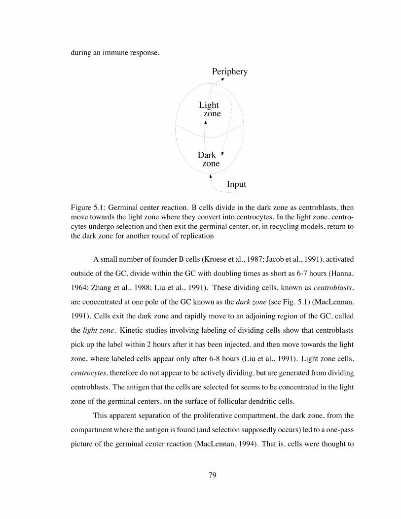
during an immune response.

Light zone

Dark zone

Input

Periphery

Figure 5.1: Germinal center reaction. B cells divide in the dark zone as centroblasts, thenmove towards the light zone where they convert into centrocytes. In the light zone, centro-cytes undergo selection and then exit the germinal center, or, in recycling models, return tothe dark zone for another round of replication

A small number of founder B cells (Kroese et al., 1987; Jacob et al., 1991), activated

outside of the GC, divide within the GC with doubling times as short as 6-7 hours (Hanna,

1964; Zhang et al., 1988; Liu et al., 1991). These dividing cells, known as centroblasts,

are concentrated at one pole of the GC known as the dark zone (see Fig. 5.1) (MacLennan,

1991). Cells exit the dark zone and rapidly move to an adjoining region of the GC, called

the light zone. Kinetic studies involving labeling of dividing cells show that centroblasts

pick up the label within 2 hours after it has been injected, and then move towards the light

zone, where labeled cells appear only after 6-8 hours (Liu et al., 1991). Light zone cells,

centrocytes, therefore do not appear to be actively dividing, but are generated from dividing

centroblasts. The antigen that the cells are selected for seems to be concentrated in the light

zone of the germinal centers, on the surface of follicular dendritic cells.

This apparent separation of the proliferative compartment, the dark zone, from the

compartment where the antigen is found (and selection supposedly occurs) led to a one-pass

picture of the germinal center reaction (MacLennan, 1994). That is, cells were thought to

79

enter the germinal center, divide in the dark zone, move into the light zone, undergo se-

lection, and the surviving cells make it into the memory compartment. The cells produced

by somatic mutation and affinity selection have large numbers of point mutations in their

immunoglobulin genes. Kepler and Perelson (1993) pointed out that accumulating random

mutations to the extent observed in the dominating, high-affinity population, without an

intervening selection event, is likely to render cells incapable of binding the antigen. They

then performed an optimal control study of affinity maturation in the GC, with the muta-

tion rate being the control variable, and concluded that cycles of mutation-less proliferation

followed by mutation and selection, are the most efficient way of creating a memory popu-

lation with a high average affinity. They suggested that one way to implement this optimal

strategy would be to have cells proliferate and then mutate in the dark zone, undergo selec-

tion in the light zone, and then return to the dark zone and repeat the process. This model

was called a cyclic re-entry or recycling model. A model based on the recycling hypothe-

sis, which took into account the architectural and kinetic details of the germinal center was

subsequently developed by Oprea and Perelson (1997). This model assumed that mutation

occurs in the replicating population of the dark zone with selection occurring in the light

zone. Affinity maturation was achieved with repeated movement between dark and light

zones.

Testing the recycling hypothesis turns out to be difficult, as we cannot, at the mo-

ment, track the cell migration patterns in the germinal centers. In this context, one might be

interested in how much affinity maturation can be achieved in a one-pass selection model.

That is, the germinal center is seeded by a few B cells, which start dividing in the dark zone,

move into the light zone to undergo selection, and then exit the germinal center, without

being able to mutate again. This is exactly the approach that van Nimwegen, Perelson and

I took, in order to give an argument ”by contradiction” for why selection must be operating

at multiple points during the germinal center reaction. Qualitatively, the results of such a

model are completely intuitive, the number of high affinity cells has an upper bound which

is given by the probability of generating such cells through mutation only. However, it

80

turns out that if the selective agent, that is the antigen, decays during the germinal center

reaction the amplification of high affinity cells is even lower than one would expect for

affinity-based selection. I think that this result gives even stronger theoretical support to

the recycling hypothesis, and also, that it is interesting on its own. There are probably a

variety of systems in which the selective agent is decreasing with time, and thus I consider

these results worth presenting.

5.2 One-pass selection model of the germinal center reac-

tion

For the specific purpose of the germinal center dynamics, one might be interested in a num-

ber of scenarios for the mutation selection process. It is, for example, not known whether

mutation occurs during B cell replication or during transcription of the immunoglobulin

gene. It is also not known whether the antigen is depleted by B cells, or by other B cell

independent mechanisms. All these scenarios give qualitatively similar results, and thus

here I will only present one: mutations are introduced at B cell replication, and the antigen

decays exponentially with time.

5.2.1 Basic model

We considered germinal center cells falling into two phenotypic classes, centroblasts and

centrocytes, and referred to these two pools of cells as the ”proliferative compartment”

and the ”selective compartment”. After mutation generates B cell variants, the interactions

among B cells, antigen and T cells, can then be thought of as a filter, selecting for the

high affinity cells, and letting the low affinity cells die. The selected cells move into the

memory pool and do not re-enter the proliferative compartment of the GC. If there is no

feedback from the selective compartment to the proliferative compartment, we can neglect

the internal dynamics of the proliferative compartment, and only consider its input into the

81

selective compartment. Thus, we assumed that, due to proliferation, there is a constant

flow of B cells into the selective compartment, where antigen is held on the surface of

follicular dendritic cells. This assumption is supported by the observation that once the

distinguishable light and dark zones could be observed on GC sections, the dark zone did

not seem to undergo further expansion (Liu et al., 1991; MacLennan, 1991), suggesting

that as cells divide half of the progeny, on average, leave the dark zone.

We group the B cells entering the selective compartment into a small number of

affinity classes (Kepler and Perelson, 1993), where all cells in class are assumed to have

similar affinity for the antigen. The number of cells of class in the selective compartment

is denoted by .

The concentration of antigen is denoted by , and I will only consider here the case

of a non-replicating antigen. Antigen within the GC is allowed to decay, the initial concen-

tration being . At any particular time in the germinal center reaction, is the

fraction of antigen remaining in the GC. While the rate of decay of antigen trapped on fol-

licular dendritic cells (FDC) is not known precisely, measurements by Tew and coworkers

(Tew et al., 1979; Tew and Mandel, 1979) and Tew & Perelson (unpublished results) using

radioactive protein antigens show approximately exponential decay with half-lives of 1 to

2 months.

We further assumed that the survival of the B cells is the result of their interaction

with the antigen, and that the rate of rescue of B cells in class is proportional to a single

factor, . This factor determines the quality of interaction of B cells in class with FDC-

associated antigen when the antigen concentration is maximal. If the antigen decays, we

assumed that the rescue rate is proportional to , the fraction of remaining antigen. One

could imagine this factor being proportional to the affinity or the binding rate constant

between cells of class and the antigen, or alternatively, it could denote the amount of

antigen that cells of class manage to present to the T cells. The amount of presented

antigen should depend on the affinity of the B cell for antigen, since B cells need to strip the

antigen off the surface of FDCs. The model is robust against the specific implementation of

82

the rescue dynamics, as long as rescue of cells in class is proportional to both the amount

of antigen with which they can interact and a single affinity class-specific factor . What

we are essentially implementing through this assumption is the view that centrocytes are

programmed to die unless ”rescued” by the interaction with antigen-loaded dendritic cells,

this interaction being affinity-dependent. From now on, the factors will be referred to as

affinities, keeping in mind that there need not be a simple mapping between these factors

and the affinity of the B cell receptors for the antigen. However, it seems reasonable to

assume that the factor is a monotonically increasing function of the affinity of cells in

class .

Let us denote the number of cells of type that have entered the memory pool by

. I will assume that these cells are long-lived on the time scale of the germinal center

reaction, such that no significant loss from this pool occurs during this time period. As I

will focus on the efficiency of the germinal center reaction itself, I will not discuss possible

dynamics of the memory cell compartment. Affinity selection, and even affinity maturation

seem to occur at post-germinal center stages (Takahashi et al., 1998). They do not, however,

affect our conclusions on the efficiency of the germinal center reaction.

Under these assumptions, the rate at which rescued cells of class enter the memory

pool is given by

(5.1)

If the antigen decays at a constant rate, , from an initial amount to at time ,

the fraction of antigen present in the GC as a function of time is simply

(5.2)

As I mentioned above, I will only present here the case of cells mutating when they repli-

cate in the dark zone. Provided that the mutation dynamics is fast with respect to the rate at

which FDC-associated antigen is depleted, and that the total influx of B cells into the selec-

tive compartment is constant over the duration of the germinal center reaction (MacLennan

et al., 1990), we can assume that there is a constant input flux, , of B cells into the light

83

zone, and that this influx has constant numbers, , of cells in the different affinity classes.

Thus, if mutation asymptotically produces a proportion of high affinity cells, then we

assume that this proportion occurs in the input to the light zone from the start of the ger-

minal center reaction. Note that this is an upper bound on the average affinity of the cells

entering the light zone since at the start of the GC reaction fewer high affinity cells might

be produced.

Once in the selective compartment, centrocytes get rescued and move into the mem-

ory pool, or die at rate . Thus, the dynamics of centrocytes of affinity class is described

by

(5.3)

The first term on the right hand side denotes the constant influx of cells of affinity class

of centroblasts into the selective compartment, the second term accounts for cell death,

and the third term for depletion of centrocytes due to their being rescued and converted

into memory cells that exit the GC. We can also take into account the possibility of lethal

mutants occurring in B cells at a rate . This would not change the above formulae but

would effectively increase the death rate .

5.2.2 Amplification of high affinity cells in the memory population is

a logarithmic function of their selection coefficient

Having described the basic model, I will now sketch the derivation of a measure of germinal

center efficiency, which I call amplification. This is defined as the ratio between the average

affinity of the memory cell pool and the average affinity of the dark zone cells. The first

ones constitute the output, the latter the input to the selective filter of the germinal centers.

The antigen dynamics is trivial and simply given by the exponential decay of equa-

tion (5.2). The B-cell dynamics is given by equation (5.3). To solve these equations, I will

assume that antigen decay is slow compared to the influx, death, and selection dynamics,

which amounts to being constant in equations (5.3). This means that during short periods

84

of time over which the antigen concentration is roughly constant, the B cells equilibrate

to the above values and that these values slowly shift under the change of as determined

by equations (5.4). Under this assumption the centrocytes will reach a quasi-steady state in

which

(5.4)

Let us now solve for the number of cells that have entered the memory pool as a

function of time for each affinity class, and for the average affinity of the output cells over

time. The output flux into the memory pool for cells in affinity class , , is given by

(5.5)

Substituting from equation (5.2) we obtain the output flux explicitly as a function of time

(5.6)

The above expressions demonstrate the main qualitative features of the model. First, the

output flux is at most as high as the input flux at any time. Obviously, when there is no

recycling or division of centrocytes, the number of cells in class entering the memory pool

cannot be larger than the influx of cells in that class. This means that if mutation only

creates a small number of cells in high affinity classes, only a small number of high affinity

cells can enter the memory pool. Second, the output flux in each class is maximal at the start

of the germinal center reaction and decays to zero at late times as antigen decays. Third,

the behavior of the output flux of class is completely independent of the affinities

and input fluxes of cells in the other affinity classes. That is, the output fluxes are not the

result of competition between cells. Rather, it is a ”competition” between rescue and death

that determines the output flux. I will briefly elaborate on this issue, as it seems somewhat

controversial at a first reading. Specifically, the notion of competition implicitly assumes

some limiting resource, which in this case would be the antigen. Preliminary simulations

of this model showed that, for biologically reasonable choices of the parameter values, the

cells will rapidly equilibrate with the free antigenic sites on follicular dendritic cells. If at

85

the end of this period there will be free antigenic sites left, then the equilibrium will slowly

shift under the independent dynamics of the antigen. If all the antigen is quickly bound by

B cells at the beginning of the germinal center reaction, I would expect that the number

of high affinity cells that will be generated will be even smaller. In this case, it would

not be guaranteed that the few high affinity variants generated during the germinal center

reaction will all get to bind the antigen to get rescued. It still seems possible though that

the amplification factor will be higher. As I will show below, the number of cells that are

generated in a one-pass selection model is already too low to account for the experimental

data. Further decreasing these numbers, even with a better amplification of high affinity

cells, does not change the basic conclusion that multiple rounds of division, mutation and

selection must take place in the germinal centers. However, in the context of a recycling

model, the limiting antigen hypothesis would clearly merit consideration.

At all times, the output flux is proportional to the input flux . As long as

, most input cells in class get rescued. As soon as , most input cells in class

die, and, as time goes on, the output flux starts decreasing exponentially at the same

rate as the antigen. This behavior is illustrated in Figure 5.2 for two affinity classes, class

being a high affinity class and class a low affinity class. The output of the zero class drops

exponentially from the start, while the output of class cells remains roughly constant for

a while and then starts dropping exponentially. Note that the time interval over which

and the output flux is roughly constant increases only logarithmically

with . This feature has important consequences for the efficiency of this type of selection

dynamics as will be discussed below. Another thing to note from Fig. 5.2 is that the output

per day can be on the order of cell or less, which makes it clear that stochastic finite size

effects should be important (for a more detailed discussion see Radmacher et al. (1998)).

Therefore, the above results should be thought to represent the average output per day, and

we expect a stochastic variant of our model to exhibit considerable fluctuations in these

numbers. These fluctuations do not, however, alter the conclusions that we can draw from

this model.

86

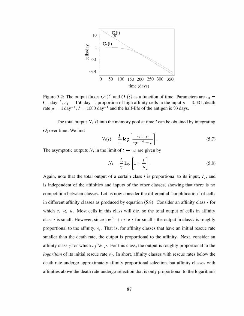
O0(t)

O1(t)

0.01

0.1

1

10

0 50 100 150 200 250 300 350ce

lls/d

aytime (days)

Figure 5.2: The output fluxes and as a function of time. Parameters areday , day , proportion of high affinity cells in the input , death

rate day , day and the half-life of the antigen is days.

The total output into the memory pool at time can be obtained by integrating

over time. We find

(5.7)

The asymptotic outputs in the limit of are given by

(5.8)

Again, note that the total output of a certain class is proportional to its input, , and

is independent of the affinities and inputs of the other classes, showing that there is no

competition between classes. Let us now consider the differential ”amplification” of cells

in different affinity classes as produced by equation (5.8). Consider an affinity class for

which . Most cells in this class will die, so the total output of cells in affinity

class is small. However, since for small the output in class is roughly

proportional to the affinity, . That is, for affinity classes that have an initial rescue rate

smaller than the death rate, the output is proportional to the affinity. Next, consider an

affinity class for which . For this class, the output is roughly proportional to the

logarithm of its initial rescue rate . In short, affinity classes with rescue rates below the

death rate undergo approximately affinity proportional selection, but affinity classes with

affinities above the death rate undergo selection that is only proportional to the logarithms

87

of their affinity. In this way, the affinity maturation that is achieved is largely set by the

death rate . If most classes have rescue rates above the selection will be very weak.

The strongest selection occurs when all affinity classes have rescue rates well below the

death rate, in which case selection is approximately proportional to affinity. In those cases

the total outputs into the memory pool will be small since most cells die. This behavior is

shown by all of the one-pass selection scenarios that I mentioned at the beginning of this

section.

Let us formally determine the efficiency of the germinal center reaction. I defined

this as the ratio of the average affinity of the memory pool at time and the average

affinity of the cells entering the selective compartment. The latter is given by

(5.9)

where is the total input into the light zone per unit time. The average affinity of

the memory pool at time is given by

(5.10)

where is the total output into the memory pool at time . The amplification factor due

to selection, , will then be

(5.11)

The asymptotic amplification is given by the limit of the above expression as

. Since we know that the most stringent selection occurs when all we can

immediately derive an upper bound for the asymptotic amplification. This will also be an

upper bound on the amplification at any time during the germinal center reaction. Relation

5.7 could be used in specific cases, when the selection coefficients of different mutants are

known, to calculate the affinity amplification at any time of the germinal center reaction.

When all , we have for the output in class

(5.12)

88

from which we can easily derive that

(5.13)

This form is typical of affinity proportional selection. The amplification is roughly propor-

tional to var(s), the variance of the input affinity distribution. In this limit case, the total

output into the memory pool , is given by

(5.14)

5.3 Implications for affinity maturation in the germinal

centers

From this one-pass selection model of the germinal center reaction, with the many variants

I analyzed, it is clear that the observed numbers of high affinity cells can only be generated

if mutant cells are selected and amplified very often during the germinal center reaction.

If, as would be expected from random mutation, there is only a very small proportion of

high affinity cells among the cells that enter the light zone, for instance on the order of

, consistent with the estimates of Radmacher et al. (1998), then only a handful of high

affinity mutants would be generated over the entire GC reaction. Note that this estimate

concerns a simple model antigen, in which one point mutation increases the affinity of

the B cell receptor by a factor of 10. If more than one point mutation were required to

produce the high affinity mutant, it becomes quite unlikely that a high affinity cell carrying

all these mutations would ever be produced. Thus, almost trivially, a low frequency of

generation of high affinity mutants restricts the output of high affinity from a germinal

center to very low numbers. One might argue that even these small numbers could be

expanded to a larger population of high affinity cells. I could envision this happening in

two ways. One would be that the selected cells do not exit the germinal center, but can

undergo further division in the germinal centers. If centrocytes do not divide, then this

scenario reduces to recycling. The second way is that there is an expansion stage between

89

the germinal center and the memory compartment. While this may well be possible, it

would only affect the amplification factor that I calculated above if this expansion were

associated with affinity selection. Otherwise, the ratio between various affinity classes

would not be affected. This case was not considered in the above model, as it would

involve a treatment of the dynamics of the memory compartment as well. There is yet

another experimental finding that makes the one-pass scenario unlikely. This is the ratio

of high affinity cells in germinal centers. While the high affinity mutation is not always

discovered within a germinal center, GCs where the high affinity mutation is found have

a high proportion of high affinity cells (Radmacher et al., 1998). If the rare high affinity

mutants are to dominate the germinal centers, assuming that they do not readily leave the

germinal centers, it is necessary that almost all germline cells die. This in turn implies that

the total cellular output from a single germinal center dominated by high affinity cells is

very low.

When all of the GCs in an animal are considered, one-pass selection can give rise

to an appreciable population of memory cells if the stringency of affinity-based selection is

low. From stathmokinetic data (Goodlad and Macartney, 1995), I can estimate that the input

into the light zone in a fully developed GC is about 1000 cells/day. If this input is sustained

for about 2 weeks of the typical 3 week GC reaction, then the 300-500 GCs reported in

the splenic response to NP-CGG (Jacob et al., 1991) would have a total light zone input of

cells. If 10% of these cells were selected (as we would obtain with the default

parameter values from the above model), then the total output from the GCR would surpass

cells. Even with some cell loss in the periphery, a reasonable size memory population

would be achieved. However, this population would consist mostly of low affinity cells. To

generate high affinity cells the stringency of selection would most likely need to be higher.

If the frequency at which high affinity cells are generated is 1 per day, and only these cells

were selected, then 300-500 germinal centers would produce of the order on to

cells. The frequency at which B cells in an unselected repertoire respond to antigen is

to . Thus, the total number of initially responding B cells in a mouse with a total of

90

B cells is to . With the higher stringency of selection needed to generate a high

affinity memory population, there would be no amplification in the number of responding

cells, contrary to the observation of both significantly higher levels of antibody production

and higher affinity in secondary responses. Again, this number would be considerably

lower if the generation of a high affinity mutant required multiple point mutations.

I would like to point out that systems in which selection is due to an agent that

decays over time are more generally encountered in the fields of immunology and infectious

disease. Thus, the intuitions built from studying the above model might prove helpful in

other situations. These may include, for example, clonal selection of B cells by a non-

replicating antigen whose concentration decreases in time, outside of the germinal center

reaction. Further examples may include adding fresh media to a culture of growing bacteria

and the spread of an epidemic. The selective agent in these cases is the nutrient, in the first

case, and individuals that are susceptible to infection, in the latter.

91

Chapter 6

Mutation rate estimation

During the germinal center reaction, mutations are introduced in the variable region of the

B cell receptor gene. Besides being so localized, mutations are also orders of magnitude

more frequent than would be expected for a random gene in evolution. Exactly how much

more frequent is difficult to estimate, because successive rounds of antigen-based selection

may take place (McKean et al., 1984; Kepler and Perelson, 1993). Accurate estimation of

mutation rates becomes essential for perturbation experiments that are designed to clarify

the role of various genetic elements (such as promoter or enhancer regions) on somatic

hypermutation.

6.1 Cell division, cell cycle times

While trying to understand the dynamics of affinity maturation of B cells during the germi-

nal center reaction, Tom Kepler and I decided to look at some simple models of cell culture

growth. We started by assuming that all genotypes are selectively neutral, and wanted to

estimate the mutation rate in the culture from the proportion of mutants found at the end of

the culture period. I wrote a simulation of such a growing culture, based on the assumption

that each cell has a certain life time, at the end of which it divides, and each of the two

progeny has a probability of being a mutant. We soon realized that the currently used

92

method for mutation rate estimation, the fluctuation analysis of Luria and Delbruck (1943),

gives an incorrect estimate of the mutation rate in any realistic culture of cells. The rea-

son is that the Luria-Delbruck (L-D) distribution assumes that all cells in the culture have

a constant probability of dividing at all times, which amounts to assuming that their cell

cycle time is exponentially distributed. This is clearly wrong for any type of cell. This

assumption, however, is necessary to make the distribution mathematically tractable. The

bias, assuming a gamma-distributed cell cycle time, can be as high as 30%. That the L-D

probability function can be in significant disagreement with the data for more realistic cell-

cycle time distributions was first pointed out by Kendall (1952). His rigorous treatment of

the problem, however, led to intractable coupled nonlinear integral equations.

What the distribution of cell cycle times is for a particular type of cell is generally

unknown, and clearly depends on a variety of external circumstances. Starved cells may

persist without dividing for long periods of time (Huisman et al., 1996), while cells that

are placed in a chemostat, with abundant supply of nutrients, continue to divide for long

periods of time (Travisano and Lenski, 1996). There are two classes of cell-cycle time

distributions that have so far been considered in modeling the experimental data. Most of

the distributions can be obtained from the gamma distribution, using different parameter-

izations. Early studies of bacterial cell growth, for example, make this assumption (Kelly

and Rahn, 1932), and possible interpretations of it are discussed by Kendall (1952). More

recent models of the cell cycle arrive at different distributions of interdivision times. Smith

and Martin (1973), for example, introduced a 2-phase model of mammalian cell cycle. Ac-

cording to this model, cells in phase of the cell cycle are viewed as being in a state

A, from which they have a constant rate per unit time, , of transition to phase B. Phase

B corresponds to the replication phase of the cell cycle, and is assumed to take a constant

time, . Another transition point has been later incorporated in this model (Brooks et al.,

1980), and variants of it with a variable B phase have also been proposed (Van Zoelen et al.,

1981). In my simulations, I explored both the case of gamma-distributed cell cycle times,

and the case of the 2-phase cell cycle.

93

In this chapter I will present improved methods for estimating mutation rates and

constructing confidence intervals, that take into account the cell-cycle time distribution.

These methods are valid for the parameter regime of , the product of the mutation rate

and culture size, being larger than 0, while , the probability of an individual cell

being mutated, being much smaller than 1. This parameter regime covers a large range of

experimental systems, while not being addressed by the extant methods of mutation rate

estimation. In particular, it covers the germinal center reaction. Although we do not have a

general form of the mutant distribution for any type of cell-cycle time distribution, we have

reached a number of important goals:

We have a order estimate of the mutation rate using the mean proportion of mu-

tants in a set of parallel cultures. This method can be used for all the cell-cycle time

distributions that we encountered.

We have a continuum approximation for the Luria-Delbruck distribution which can

be calculated more easily than the discrete distribution. The experiments that are

designed for mutation rate estimation seem to fall largely in the parameter range

for which the continuum approximation holds (see for example Lea and Coulson

(1949)).

We found a way to parameterize the continuum Luria-Delbruck distribution for cul-

tures of cells that have a 2-phase cell cycle. The parameters depend only on the

cell-cycle time distribution, and are independent of the mutation rate and cell culture

size. This allows us to design a general method for constructing confidence intervals

for the mutation rate in this type of cell cultures.

We found that, if the cell cycle time is gamma-distributed with a given shape param-

eter, the 5 and 95 percentile values of the proportion of mutants in cultures of known

size scales linearly with the mutation rate. I estimated the parameters for the linear

fit for cell culture sizes in the range of cells. This is below the experimen-

tal range of bacterial culture sizes, but it approaches the culture size for eukaryotic

94

cells. I show how to construct the confidence interval for the mutation rate in this

parameter range. However, we are continuing this work, with the goal of finding a

culture-size independent method of mutation rate estimation for cultures of cells with

gamma-distributed cell cycle times.

Given these results, we are in the position of improving the methodology of mutation rate

estimation.

I will first describe the computational model that I designed for testing our theoreti-

cal predictions, and for fitting the parameters of the generalized continuum Luria-Delbruck

distribution. I will then outline the derivation of the mean proportion of mutants in a culture

of a given size, and I will show that the theoretical predictions are well fitted by simulation

data.

I will next introduce the continuum approximation of the Luria-Delbruck distribu-

tion, due to T. Kepler (Kepler & Oprea, in preparation). This represented the basis for

most of our further explorations. I will describe the parameterization that we designed for

extending this distribution to fit the simulation data for 2-phase cell cycle times.

I will then show that for gamma-distributed cell cycle times, the 5 and 95 percentile

values of the distribution of the proportion of mutants scales linearly with the mutation rate.

Thus, even for a culture of cells with gamma-distributed cell cycle, as long as the culture

size is not larger than , we can still construct confidence intervals for the mean.

Finally, I conclude with a discussion of other issues that arise in estimating mutation

rates in bacterial cultures and germinal centers, and I propose ways to circumvent these

problems.

6.2 Computational model of a growing culture of cells

The problem that I am trying to solve is to estimate the mutation rate in a culture of cells

which is undergoing exponential growth and phenotypic mutations. The basic setup as-

sumed by fluctuation analysis is the following. A culture is seeded with (generally 1)

95

cells. The culture then grows exponentially up to cells. When a wildtype cell divides,

each of its progeny has a probability of undergoing a mutation that changes its pheno-

type. In bacteriological experiments, the change in phenotype generally means that the cell

will be capable of using a nutrient that a wildtype cell could not metabolize. However,

the assay for detecting the mutants is only performed after the growth of the culture. That

means that, while the culture is growing, mutant cells do not have a selective advantage

over wildtype cells. They grow at the same rate as wildtype cells. It is also assumed that

mutants do not revert to the wildtype phenotype, and thus all progeny of a mutant cell

will be mutants. When the culture has reached size , we count the number of mutants,

. Note that lethal mutations are neglected in this analysis. In fact, all the mathematical

treatments of this process neglect lethal mutations, as they probably affect only the growth

rate of the culture, not the relative proportion of mutant and wildtype cells. Also, neutral

mutations fall under the wildtype phenotype, so they do not need a separate mathematical

treatment. The question is now, if we have a number of data points ( ), from different

cultures that all have presumably the same mutation rate, how do we estimate the mutation

rate from these data?

I set up an event driven simulation of the process that I just described. Each cell is

represented by an object characterized by its phenotype, wildtype or mutant, and a division

time. I seed the system with one wildtype cell of age 0. When a new cell object is created,

I assign it a cell cycle time. I explored both types of cell-cycle time distributions that

have been used in the literature. The first is the gamma distribution of order , and scale

parameter :

(6.1)

The mean cell cycle time is and its variance . For simplicity, I set the

scale parameter to 1 in all cases. This will only be reflected in the absolute values of the cell

cycle time, not in their relative ordering. The second type of cell-cycle time distribution

that I used I call shifted exponential. That is, there is a constant probability per unit time

that the cell starts to divide, , but division takes a constant amount of time for all cells,

96

. Then the distribution of cell cycle time is

if

otherwise(6.2)

The mean cell cycle time is in this case , and the variance in cell cycle time is

. I scaled these parameters such that the mean cell cycle time is 1. That is, only the

ratio between the division time and the mean waiting time between two divisions will affect

the mutant distribution in the culture, not the absolute values of these times. I will denote

this parameter by

(6.3)

I maintain a priority queue of cell objects, the value used for determining the order

of objects in the queue being the absolute value of time at which the cell divides. This

in turn is the sum of the cell cycle time of the cell and the time at which the cell was

born. At each step of the simulation, the object with the lowest time of division is removed

from the queue. Two new objects are created, each having a division time which is the

sum of the current time and a cell cycle time drawn from the gamma distribution. With

probability each of the two daughter cells mutates. These operations are performed for

a fixed number of steps, i.e., for duplications, if we are to achieve a culture of size

. This algorithm implements the dynamics of a culture that grows exponentially from 1

to cells. Random deviates from a gamma distribution of a given order were generated

using the standard Numerical Recipe function (Press et al., 1988). The special case of the

shape parameter gives us deviates from the exponential distribution. At the end of

the simulation, I count the number of mutants among the cell objects. I generate a large

number ( ) of replicates of this experiment for constructing the distribution of the

proportion of mutants in the culture.

97

6.3 Mean number of mutants in a culture of size

For calculating the mean number of mutants in the culture, we used the following approach.

We determined the mean number of division events that a cell in the final culture has expe-

rienced on the path from the cell that seeded the culture to a cell in the culture of size .

We then calculated the probability that a mutation occurred along this path.

To determine the mean number of divisions, we first determined the growth rate in

the culture as a function of the cell-cycle time distribution, and then we used it to determine

the mean generation number of a cell in the final culture. I will first outline the derivation

of the growth rate in the culture. The age at which any individual cell divides is a random

variable, . For a cell randomly chosen at birth, this age of division is described by the

cumulative distribution function defined by Prob( = , and, equivalently, by

its density function .

At division, the parent is lost and two cells of age zero are created. Consider a

population of such cells. If the density of cells of age in the population is denoted

where is the absolute time, then the equation for loss of the parent cells by division is

(6.4)

where is given by

(6.5)

Note that we can write

(6.6)

The equation for gain of new cells is derived by integrating Eq.(6.4) over and demanding

that the total rate of production be given by

(6.7)

This results in the production equation

(6.8)

98

We seek solutions to Eq.(6.4) of the form , the so-called separable solu-

tions. Substituting this form into Eq. (6.4), we obtain

(6.9)

Note that the right-hand side depends only on , while the left-hand side depends only on

. Therefore, if this equation is to hold for all values of both and , then either side must

be constant. If we call this constant , we have

(6.10)

and

(6.11)

The solution for is simply

(6.12)

while for we have

(6.13)

The condition on is obtained by substituting Eq. (6.13) into Eq. (6.8) to give

(6.14)

Now an integration by parts and use of Eq. (6.6) yields

(6.15)

This is the eigenvalue equation for that we seek. Since is the density function for

cell-cycle time, we can write this last result as

E (6.16)

where E denotes expectation with respect to . If is a gamma distribution of shape

parameter and mean (Eq. 6.1), then the growth rate is given by

(6.17)

99

Note that in the limits that we understand a priori, we have agreement with our expecta-

tions. For , corresponding to an exponential density function, we should recover a

simple Markov model. In this case, we get . For the limit as , we get a

process describing a polymerase chain reaction, with all ”cells” replicating at exactly equal

times. For this we have . Both of these results conform to prior knowledge.

The calculation of the mean generation number requires us calculating the mean

age of a cell at division. For this, we assume that the culture was in stationary growth from

the beginning. That is, we assume that the age distribution in the culture is constant as a

function of time. We then calculate the average age at division using the density function

for age, , but weighted by the proportion of cells of age in the culture. To determine

this, observe that cells that divide, by chance, earlier than usual, will leave, on average,

more offspring than those that divide later. If the growth rate is , i.e., the number of cells

grows like , then two cells that divide time units apart will leave

different numbers of offspring and the ratio in that number is . For the simplicity

of notation, I will denote . Following this argument, first given by Fisher

(1930), we obtain the average age at division

E EE

(6.18)

but in light of the definition of , we get

E E (6.19)

For the specific case of the gamma distribution, parameterized as above

E (6.20)

The mean number of divisions is given by

EE E

(6.21)

which again in the case of the gamma distribution gives

E (6.22)

100

For the exponential distribution, and for the PCR process,

.

We may now calculate the mean number of mutants by assuming that at each cell

division, each of the daughters has a probability of becoming mutant (and therefore all of

her daughters as well). The probability that no mutation occurs in divisions is ,

so the probability that at least one mutation occurs is . Then the probability

of a cell being a mutant is , where is the probability that the

cell underwent divisions. For small mutation rates, such that , this expression

can be approximate by , that is, the probability that an individual cell is mutant is

E . Each of the cells in the final culture has this chance of being a mutant, thus the

mean number of mutants in the culture is E . For a gamma distribution of

cell-cycle times, this becomes

(6.23)

where the correction factor is given by

(6.24)

We now have an analytical form for the mean number of mutants in a culture of size , in

which the cells have a gamma-distributed cell cycle time.

A similar derivation gives us the correction factor for the mean in the case of a

2-phase model of cell cycle time. Assume that the cell cycle time has a constant compo-

nent, , and an exponentially distributed part, of parameter . Thus, the cell-cycle time

distribution isif

otherwise(6.25)

The mean cell cycle time is , and the variance in cell cycle time is . The

coefficient of variation of this cell-cycle time distribution is

101

Let us derive the mean proportion of mutants in the culture with this new cell-cycle time

distribution. Assuming that the culture is in stationary growth, with growth rate , the

number of cells in the culture as a function of time is given by

Conform Eq. 6.15, the eigenvalue equation for the growth rate is

where is the distribution of the age of cells at division. For the shifted exponential

cell-cycle time distribution,

Thus must satisfy

(6.26)

The solution of this equation can be given in terms of the Lambert’s W function:

(6.27)

The average age at division of a cell on the lineage from the root to a leaf in the genealogical

tree of the culture is given by Eq. 6.18:

From the eigenvalue equation for , we find (Eq. 6.19)

The average number of generations from the founder cell to a cell in the current culture is

then given by

102

Now

This can be expressed in a simpler form, given that the growth rate, satisfies Eq. 6.26.

Namely,

As before, if we write the mean number of mutants in the culture as

where is a function of the cell-cycle time distribution, for the shifted exponential we

obtain:

(6.28)

As expected, if we set , we obtain , which is the correction factor for

exponentially-distributed cell cycle time.

The mean proportion of mutants as obtained from simulations, together with the

theoretical prediction is presented in Tables 6.1 (for the gamma-distributed cell cycle time)

and 6.2 (for the shifted exponential). 10000 independent runs were performed for each of

the parameter sets.

As can be seen from the tables, there is a good agreement between the means that I

obtained from simulations, and the ones that I calculated. It is also apparent that if the cell

cycle is exponentially-distributed, the mean proportion of mutants is higher, for the same

mutation rate per division, than if the cell-cycle time distribution had a higher order. Turn-

ing the argument around, if we assume that the cell cycle time is exponentially-distributed,

when in reality it is not, leads to underestimation of the mutation rate. Although this comes

out of the expression for the mean, I would like to give an intuitive argument for how the

cell-cycle time distribution enters into the mutant distribution.

Assuming that the cells have an exponentially-distributed cell cycle time is equiv-

alent to assuming that they all have a constant probability of dividing per unit time. This

103

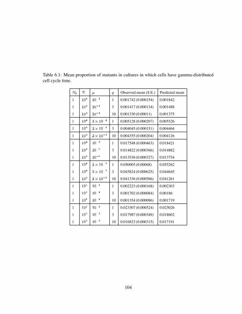
Table 6.1: Mean proportion of mutants in cultures in which cells have gamma-distributedcell cycle time.

Observed mean (S.E.) Predicted mean

1 1 0.001742 (0.000154) 0.001842

1 3 0.001417 (0.000134) 0.001488

1 10 0.001330 (0.00011) 0.001375

1 1 0.005128 (0.000207) 0.005526

1 3 0.004045 (0.000151) 0.004464

1 10 0.004355 (0.000204) 0.004126

1 1 0.017548 (0.000463) 0.018421

1 3 0.014822 (0.000366) 0.014882

1 10 0.013536 (0.000327) 0.013754

1 1 0.050005 (0.00068) 0.055262

1 3 0.043824 (0.000625) 0.044645

1 10 0.041336 (0.000586) 0.041261

1 1 0.002223 (0.000168) 0.002303

1 3 0.001702 (0.000084) 0.00186

1 10 0.001354 (0.000086) 0.001719

1 1 0.023307 (0.000524) 0.023026

1 3 0.017987 (0.000349) 0.018602

1 10 0.016823 (0.000315) 0.017191

104

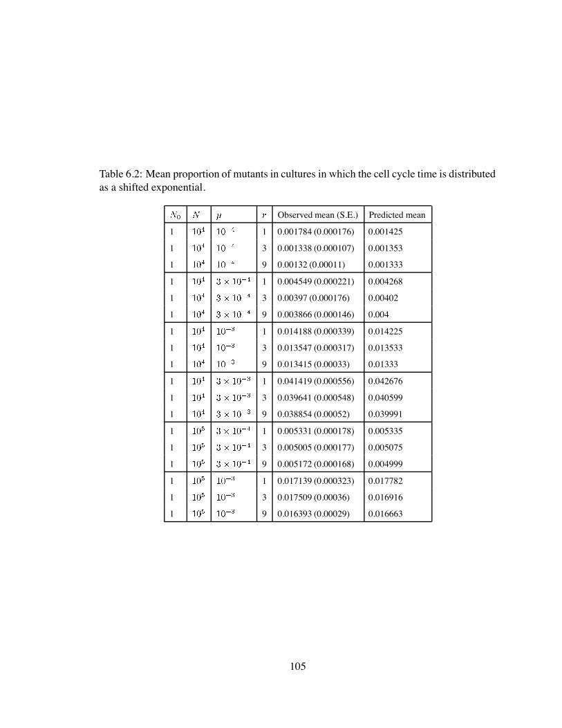
Table 6.2: Mean proportion of mutants in cultures in which the cell cycle time is distributedas a shifted exponential.

Observed mean (S.E.) Predicted mean

1 1 0.001784 (0.000176) 0.001425

1 3 0.001338 (0.000107) 0.001353

1 9 0.00132 (0.00011) 0.001333

1 1 0.004549 (0.000221) 0.004268

1 3 0.00397 (0.000176) 0.00402

1 9 0.003866 (0.000146) 0.004

1 1 0.014188 (0.000339) 0.014225

1 3 0.013547 (0.000317) 0.013533

1 9 0.013415 (0.00033) 0.01333

1 1 0.041419 (0.000556) 0.042676

1 3 0.039641 (0.000548) 0.040599

1 9 0.038854 (0.00052) 0.039991

1 1 0.005331 (0.000178) 0.005335

1 3 0.005005 (0.000177) 0.005075

1 9 0.005172 (0.000168) 0.004999

1 1 0.017139 (0.000323) 0.017782

1 3 0.017509 (0.00036) 0.016916

1 9 0.016393 (0.00029) 0.016663

105

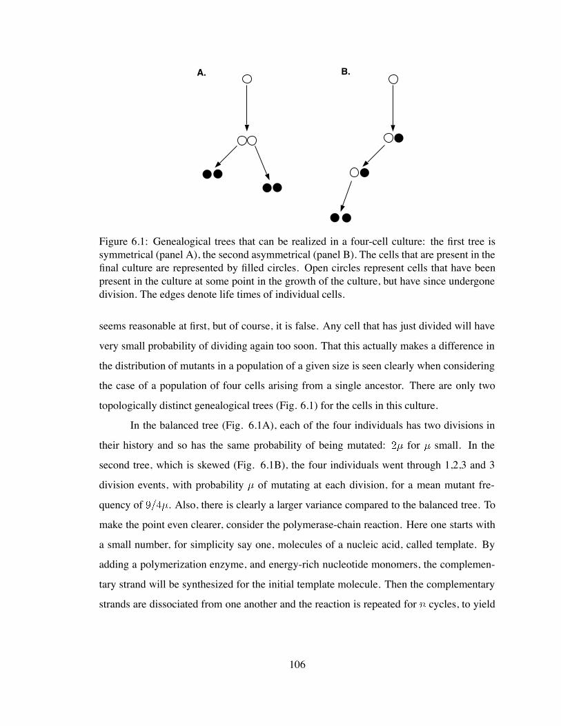
A. B.

Figure 6.1: Genealogical trees that can be realized in a four-cell culture: the first tree issymmetrical (panel A), the second asymmetrical (panel B). The cells that are present in thefinal culture are represented by filled circles. Open circles represent cells that have beenpresent in the culture at some point in the growth of the culture, but have since undergonedivision. The edges denote life times of individual cells.

seems reasonable at first, but of course, it is false. Any cell that has just divided will have

very small probability of dividing again too soon. That this actually makes a difference in

the distribution of mutants in a population of a given size is seen clearly when considering

the case of a population of four cells arising from a single ancestor. There are only two

topologically distinct genealogical trees (Fig. 6.1) for the cells in this culture.

In the balanced tree (Fig. 6.1A), each of the four individuals has two divisions in

their history and so has the same probability of being mutated: for small. In the

second tree, which is skewed (Fig. 6.1B), the four individuals went through 1,2,3 and 3

division events, with probability of mutating at each division, for a mean mutant fre-

quency of . Also, there is clearly a larger variance compared to the balanced tree. To

make the point even clearer, consider the polymerase-chain reaction. Here one starts with

a small number, for simplicity say one, molecules of a nucleic acid, called template. By

adding a polymerization enzyme, and energy-rich nucleotide monomers, the complemen-

tary strand will be synthesized for the initial template molecule. Then the complementary

strands are dissociated from one another and the reaction is repeated for cycles, to yield

106

molecules of nucleic acid. At each cycle, all the molecules in the vat act as templates,

and the complementary strand is synthesized for each of them. It is clear that only the com-

pletely balanced tree will be realized in this type of reaction. Theoretically, the probability

of obtaining a given genealogical tree can be computed given the distribution of cell cycle

times. The proportion of mutants in the final culture will depend only on the relative prob-

abilities of realizing different types of genealogical trees with the same number of leaves,

and on the probability of mutation at cell division. The problem is that this computation

becomes intractable for even very small trees.

The approach that we eventually designed for accounting for the cell cycle time in

the growth of the culture was suggested by our findings that:

the mean proportion of mutants depends on the growth rate of the culture, and

that the growth rate is only a function of the cell cycle parameters.

Analyzing the empirical distributions of mutants that we obtained for various cell cycle

parameters, we found that they closely resemble in shape the Luria-Delbruck distribution.

This prompted us to attempt to generalize a variant of the Luria-Delbruck distribution for

cell-cycle time distributions other than exponential. This variant is a continuum approxi-

mation of L-D, due to my collaborator, T. Kepler (Kepler & Oprea, in preparation). In the

next section, I present a brief outline of the derivation of this distribution.

6.4 Continuum approximation of the Luria-Delbruck dis-

tribution

The Luria-Delbruck distribution came out of a study designed to test whether mutations in

a bacterial population subject to strong selection arise in response to the selective agent, or

independently of it. The distribution of the number of mutants, , in a culture of size ,

that has been grown under conditions in which these mutations did not confer a selective

advantage to the cells bearing them, came to be known as the Luria-Delbruck distribution.

107

It constitutes the basis for mutation rate estimation using the so-called ”fluctuation analy-

sis”. Such an experiment involves growing a number of bacterial cultures from one cell to a

final culture size , and estimating the number of mutants in each of the parallel cultures.

The mean or median number of mutants, or the proportion of cultures with no mutants

are the statistics generally employed for mutation rate estimation. Fluctuation analysis has

been applied to the study of mutational processes not only in prokaryotic, but also eukary-

otic genomes (Jones et al., 1994). The mathematical study of the L-D distribution, initiated

by Luria and Delbruck themselves, was elaborated by Lea and Coulson (1949); Bartlett

(1978); Kendall (1948). More recently, a revisiting of the mutational processes in bacteria

initiated by Cairns et al. (1988) caused another wave of mathematical exploration of the

L-D distribution (Stewart et al., 1990; Sarkar, 1992; Jones et al., 1994). These efforts made

the numerical computation of the L-D distribution reasonably efficient, though no closed

form solution for it has been found.

In section 6.2, I described the basic setup for fluctuation analysis, which I used to

construct my computational model. This setup is assumed in the derivation of L-D as well,

with the restriction that at any moment, all replicators have equal probability of dividing.

This can be shown to be equivalent of assuming an exponential distribution for the cell

cycle time (recall that in my simulations I allowed for more general forms of the cell cycle

time distribution). If we work in the regime where the product of mutation rate and culture

size, , is large, but the product , giving the probability that any given cell is

a mutant, is small, we can use the following approximation. Instead of taking the number

of mutants, as the random variable of interest, we take the proportion of mutants in the

culture, , and approximate it as a continuous random variable. The validity

of this approximation follows from the prior assumption . We then determine

the density function for , and attempt to generalize this distribution for non-exponential

cell-cycle time distributions.

We start from the generating function of the Luria-Delbruck distribution, defined as

E (6.29)

108

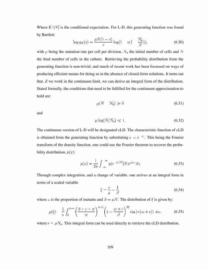
Where E is the conditional expectation. For L-D, this generating function was found

by Bartlett:

(6.30)

with being the mutation rate per cell per division, the initial number of cells and

the final number of cells in the culture. Retrieving the probability distribution from the

generating function is non-trivial, and much of recent work has been focussed on ways of

producing efficient means for doing so in the absence of closed-form solutions. It turns out

that, if we work in the continuum limit, we can derive an integral form of the distribution.

Stated formally, the conditions that need to be fulfilled for the continuum approximation to

hold are:

(6.31)

and

(6.32)

The continuum version of L-D will be designated cLD. The characteristic function of cLD

is obtained from the generating function by substituting . This being the Fourier

transform of the density function, one could use the Fourier theorem to recover the proba-

bility distribution, :

(6.33)

Through complex integration, and a change of variable, one arrives at an integral form in

terms of a scaled variable

(6.34)

where is the proportion of mutants and . The distribution of is given by:

(6.35)

where . This integral form can be used directly to retrieve the cLD distribution.

109

6.4.1 Cell-cycle correction to the continuum Luria-Delbruck distribu-

tion for 2-phase models of the cell cycle

Recall that cLD is obtained starting from the Bartlett generating function, which is the

generating function corresponding to the Luria-Delbruck distribution. Also recall that the

mean proportion of mutants can be expressed as , where the correction factor

only depends on cell cycle parameters. We may view in this formula as the effective mu-

tation rate. This observation prompted us to attempt to generalize cLD for non-exponential

distributions of cell cycle times. The approach is essentially to replace by the effective

mutation rate . It turns out that, for cell cycle times that are distributed as a shifted expo-

nential, this is not sufficient to give us mutant distributions that fit the experimental ones.

However, if we also assume that the effective number of initial (and final) number of cells

in the culture is (and ), we can obtain very good fit between the simulation

data and the theoretical prediction. Note that here I grouped together the correction factor

for the mutation rate and the correction factor for the number of cells in one parameter

. For the correction factor for the mutation rate we have an analytical expression. The

correction factor for the cell number we have to determine by fitting the simulation data to

the generalized form of cLD.

I will describe the fitting procedure for the parameter . It turns out that the value

of this parameter is determined by the ratio of the division time ( ) to the mean waiting

time ( ). It is not affected by the mutation rate or the final number of cells in the culture.

The major implication of this result is that we can obtain the value of this parameter for

any of interest by simulating cultures with relatively small numbers of cells. We can then

use this value for any culture size, and thus infer mutation rates in realistic-size cultures.

In the integral form of the distribution, we let and . The scaled

variable becomes

(6.36)

We then perform a one-parameter optimization, using as criterion for the goodness of fit

110

the value. The procedure is the following. We generate the empirical distribution of the

proportion of mutants (and the corresponding cumulative distribution) from the simulation

data. This will also give us the distribution of the variable , which is related to the pro-

portion of mutants, , through Eq. 6.36. is the correction factor due to the cell cycle time

distribution (Eq. 6.28), is the final number of cells in the culture, is the mutation rate

that we used in the simulation, and is the parameter that we need to identify. We may use

as a first choice for its value for the L-D distribution, which is 2. Let denote the

empirical cumulative distribution of . Let be the theoretical cumulative distribution

of this variable. We can calculate this distribution using the integral form of Eq. 6.35, with

parameters , and . The quantity that we want to minimize is the

value, calculated as:

(6.37)

where takes values as given by Eq. 6.34, with the proportion of mutants varying between 0

and 1, in increments of . In fact, we neglected the cumulative density values below 0.01

and beyond 0.99 (in a few cases 0.98 or 0.97). They do not affect the fit significantly, while

the computation of the integral becomes difficult in these regions. Also, the simulation

data is less precise in these regions, as we would need a very large number of runs to be

able to see events that have a very low probability. We find that value of the parameter

that minimizes the value. The algorithm for minimization is the Golden Section Search

algorithm, described in Press et al. (1988). Table 6.4.1 gives these values for a number of

data sets. Note that , , and are the values that we used in the simulations. ,

, and are the effective initial number of cells, final number of cells, and mutation

rate. The cases where we truncated the right-hand tail at proportions different from 0.99

are marked.

The first three data sets in the table correspond to cultures based on exponential

cell-cycle time distribution. As we expect, the value of the parameter for all these data

sets is around 2. As the division time becomes a larger proportion of the cell cycle,

the value of the parameter increases. However, the most dramatic change occurs when

111

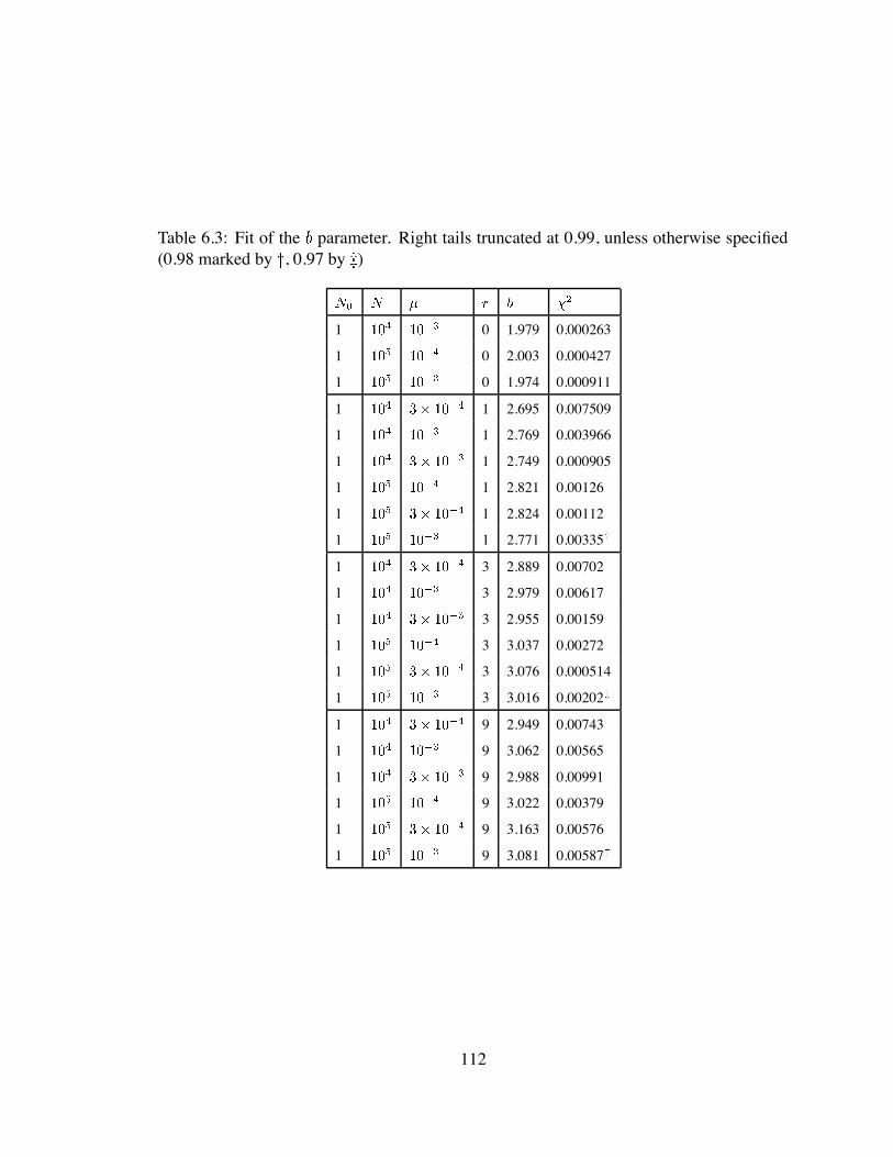
Table 6.3: Fit of the parameter. Right tails truncated at 0.99, unless otherwise specified(0.98 marked by , 0.97 by )

1 0 1.979 0.000263

1 0 2.003 0.000427

1 0 1.974 0.000911

1 1 2.695 0.007509

1 1 2.769 0.003966

1 1 2.749 0.000905

1 1 2.821 0.00126

1 1 2.824 0.00112

1 1 2.771 0.00335

1 3 2.889 0.00702

1 3 2.979 0.00617

1 3 2.955 0.00159

1 3 3.037 0.00272

1 3 3.076 0.000514

1 3 3.016 0.00202

1 9 2.949 0.00743

1 9 3.062 0.00565

1 9 2.988 0.00991

1 9 3.022 0.00379

1 9 3.163 0.00576

1 9 3.081 0.00587

112

changes from being negligible, to being as large as the mean waiting time. The other

parameter of these distributions, , shows a similar behavior. The effective mutation rate is

maximal for , it decreases with , with the most dramatic change occurring at the

transition between and .

6.4.2 Inference procedures.

I will outline the procedure that we can use for constructing confidence intervals for the

mutation rate using the parameterized distribution that I described in the previous section.

Assume that we start with a datum , representing the proportion of mutants in the

culture, and the we know parameter of the cell cycle time distribution. Knowing , we can

first calculate the growth rate of the culture, using Eq. 6.27 determine, with

and . We then calculate , the correction for the mutation rate, by the formula

6.28. We retrieve the value of the parameter from Table 6.4.1. We can calculate the value

of the scaled variable as a function of the mutation rate

(6.38)

Assume that we want to find the confidence interval for the mean. All we need

to do is to find the values of the mutation rate for which the given datum corresponds

to the and quantiles, respectively, of the distribution specified by the formula

6.35. As the quantile to which corresponds is a monotonic function of , a simple search

algorithm on would give us these values.

This procedure can be easily automated. The interface to it would be simple, the

query being specified by only two variables: the ratio of the division time to the mean

waiting time (or, even simpler, the coefficient of variation of the cell cycle time), and the

observed proportion of mutants in the culture. The program would construct confidence

intervals for the mutation rate. I believe that this approach would provide a very useful tool

in the study of mutational processes.

113

6.5 Constructing confidence intervals for the mean muta-

tion rate in cultures of cells that have a gamma-distributed

cell cycle time

Mutant distributions in cultures in which the cells have a gamma-distributed cell cycle time

are not amenable to the same type of parameterization that I described in section 6.4.1.

Thus, at the moment we do not have an expression for these distributions that we could use

in estimating the mutation rate using the above method. We have, however, explored the

behavior of the mutant distributions that we obtain from our simulations. We found some

properties that allow us to construct a confidence interval based on the observed mean

proportion of mutants. The approach is the following.

We construct the mutant distribution empirically, through simulation. The limiting

factors are the running time and the memory taken up by the cell objects. Constructing a

culture of size requires division events. The problem for large culture sizes is

two-fold. Not only does it take longer to simulate the culture growth, but also the number

of independent runs that we would have to do to obtain an accurate distribution becomes

larger.1 Cultures of size can, nonetheless, be simulated on the currently available

workstations. Thus, for the germinal center reaction, in which the number of cells does not

surpass , we can still simulate the growth of the cell population.

As I mentioned before, when the cell cycle time is gamma-distributed, only the

order parameter of the gamma distribution determines the relative probability of realizing

different genealogical trees. I denoted this parameter by . For a given , I generated

independent runs for each value of (either or cells) and each value of the

mutation rate. I then investigated the behavior of the quantiles of the distribution of the

proportion of mutants. Let and denote the 5 and 95 quantiles, respectively, and1Using a Sun Ultra2 2300, 300 MHz processor, running SunOS 5.5.1, one run of cells takes 8 seconds

and 3.7MB RAM. The complexity of the algorithm is O( ), as it amounts to constructing the priorityqueue of cell objects. However, we have to do of the order runs to obtain the distribution, thus thecomplexity of the algorithm for constructing the distribution is at least O( ).

114

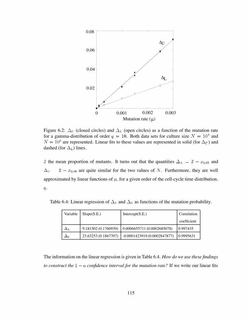
!L

!U

0.02

0.04

0.06

0.08

Mutation rate (µ)0.0000 0.0010 0.0020 0.00300 0.001 0.002 0.003

Figure 6.2: (closed circles) and (open circles) as a function of the mutation ratefor a gamma-distribution of order . Both data sets for culture size and

are represented. Linear fits to these values are represented in solid (for ) anddashed (for ) lines.

the mean proportion of mutants. It turns out that the quantities and

are quite similar for the two values of . Furthermore, they are well

approximated by linear functions of , for a given order of the cell-cycle time distribution,

.

Table 6.4: Linear regression of and as functions of the mutation probability.

Variable Slope(S.E.) Intercept(S.E.) Correlation

coefficient

9.181502 (0.1760939) 0.0006655711 (0.0002685078) 0.997435

23.63253 (0.1867707) -0.0001423919 (0.0002847877) 0.9995631

The information on the linear regression is given in Table 6.4. How do we use these findings

to construct the confidence interval for the mutation rate? If we write our linear fits

115

as

(6.39)

(6.40)

then the confidence interval on is given approximately by the bounds

(6.41)

and

(6.42)

where is the observed proportion of mutants in the culture and is the correction factor

for the mean, given by the cell cycle parameters.

6.6 Estimating mutation rates in real cultures

6.6.1 Bacterial growth

I will return now to the question of mutation rate estimation in bacterial cultures. Luria-

Delbruck fluctuation analysis is generally used to estimate the rate of so-called growth-

dependent mutations in bacterial cultures. These are to be distinguished from adaptive

mutations that occur in slowly growing cultures, in which little cell division takes place

(Torkelson et al., 1997). The distinction seems to be mostly in terms of the mutational

mechanism. In the first case, the spectrum of observed genetic changes seems to be much

more heterogeneous, and thus believed to occur via multiple mechanisms, whereas adap-

tive mutations are similar in various cells or systems, and have been related to recD gene

activity.

Restricting ourselves to mutations that occur in growing cultures, we saw that the

assumption that underlies the L-D distribution of mutants, namely that the cell cycle time

is exponentially distributed, results in underestimation of the mutation rate. In the above

116

sections I provided improved methods that take into account the cell-cycle time distribution.

There are a number of other sources of errors that I would like to briefly discuss here.

In my simulations, I can precisely count the mutants when the culture reaches

size . In fluctuation analysis experiments, one cannot decide individually for each cell

whether its phenotype is wildtype or mutant. The number of mutants is estimated by tak-

ing a sample of the culture, growing it on a selective environment, that only supports the

growth of the mutants, and counting the number of colonies. Each colony is assumed to

have been seeded by one mutant cell. Jones et al. (1994) discusses to a large extent the

statistical complications associated with estimating the number of mutants in the culture.

One issue which is not addressed in their study, is the assumption that the cells were in

exponential growth over the whole period of the experiment. Such a condition is difficult

to ensure. After growing exponentially, a bacterial culture generally experiences significant

cell death, after which a stationary phase settles in. Although I will not go into the details

of correcting for the cell death at the end of the exponential phase, as this would require

detailed knowledge of the mechanisms involved, I will outline the procedure for a simple

case. The basic assumption would be that death affects with equal probability wildtype and

mutant cells. Then what we need to know in order to infer the mutation rate is the cell-cycle

time distribution, and the counts of viable and dead cells at the time of mutant detection.

The distribution of mutants in the final culture can be obtain from the convolution of the

distribution at the end of exponential expansion and the hypergeometric distribution, cor-

responding to the sampling realized by the death process. That is, if mutants and wildtype

cells are equally likely to be affected by death, the set of viable cells is essentially a sample,

without replacement, of the cells at the end of the phase of exponential growth.

I believe that at this moment we have the basic components for an accurate method

for mutation rate estimation in bacterial cultures. Automating this method is one of my

topics of future work.

117

6.6.2 Emergence of high affinity mutants in the germinal centers

Our initial motivation for improving mutation rate estimation techniques was to estimate

mutation rates in germinal centers. Compared to the simple computational model that I

designed for a bacterial culture, the cell population dynamics in the germinal centers is

complicated by a number of factors:

Germinal centers have an initial phase of exponential expansion of cells, which is

followed by an apparent steady-state in cell number. During this phase there is con-

siderable cell death, as well as clonal expansion.

Cells grow in a selective environment. Certain mutations are advantageous, and of

these, some result in preferential expansion of the clone (Radmacher et al., 1998). At

the moment we have no quantification of the selective advantage of these clones, and

we do not know by what mechanism their rapid expansion occurs.

Deleterious mutations can also be generated, and they seem to be relatively rapidly

followed by the death of the cell.

These constraints make it extremely difficult to attempt an accurate estimate of the mutation

rate in germinal centers. An approach that is used experimentally in order to circumvent

the selection problem, is to look at passenger genes in B cells that went through a somatic

mutation process. A passenger gene is a gene that does not affect the survival probability

of the cell in a particular environment. In our case, this environment is the germinal center.

The claim is that the association of the passenger gene with a successful or unsuccessful

phenotype, that is, with a high or low affinity immunoglobulin receptor is irrelevant. If

we focus on one site (nucleotide position) of the passenger gene, the mutant distribution

only depends on the relative probability of generating different tree shapes (and, of course,

on the probability of mutation per cell replication, assuming that mutations are replication-

dependent). This is what we found in the analysis of the L-D distribution. If the association

between the passenger gene and a successful or unsuccessful phenotype were relevant, then

118

the relative probabilities of different trees would have to be modified by this association. It

is conceivable that successful mutants are selected faster and/or divide at faster rates than

unsuccessful ones. Then if the cell harbors a successful mutation, its cell cycle time may

have a different distribution than if the cell did not have this mutation. If this were the case,

the number of generations that a cell goes through would depend on its selected receptor.

Thus, it is not clear that measuring the mutation rate from passenger genes that are carried

by cells that have functional, selected receptors, circumvents the selection problem.

However, looking at this experiment differently allows me to design a mutation

rate estimation method based on passenger gene mutation. Let us assume that up to the

point when the successful mutant appeared in the germinal center, the cells underwent

exponential expansion, with cells cycle times being independent, identically-distributed

random variables. The consistency of the estimate of the waiting time for a successful

mutant (Radmacher et al., 1998) and of the duration of the exponential expansion phase

of the germinal center reaction (Liu et al., 1991) support this hypothesis. Let us further

assume, similar to Radmacher et al. (1998), that the progeny of this successful mutant will

take over the germinal center.

Now consider the germinal center cells at the end of germinal center reaction. Se-

quencing their passenger gene and taking the intersection of the mutation sets in these

genes, we should obtain the set of mutations that were present in the founder cell of the

clone that stumbled upon the successful mutation. So the set of mutations in the passenger

gene of this founder gives us an estimation of the number of mutations in a cell at the end

of the exponential expansion phase.

I will now define the quantities that I need for estimating the mutation rate from

these data:

= probability that a cell in a culture of size is of generation . I will

assume that the generation number of the cell that finds the key mutation when the

culture reached size is the average generation number in the culture at that time.

To be accurate, we would have to exclude the cells in the culture whose sister cells

119

divided already. They cannot be recently born, and the mutation can only be in a

recently born cell. This density function is completely determined by the cell cycle

parameters, and I can determine it by simulation.

= probability that the genealogical tree of the culture is of size when the

successful mutation is found. A tree of size is generated by divisions.

With a constant mutation rate per division, the probability of finding the successful

mutant will only be related to the tree size, not to the tree shape. Specifically, let us

assume that the successful mutant is only one mutation away from the germline. Let

be the probability of a mutation per site per division. Let be the probability that

a mutation at the site of interest produces the appropriate nucleotide (I will assume

for the moment that all nucleotides have an equal chance of being produced by a

mutation). Then the probability that the mutation occurred at the division is

Note that I neglect here the deleterious mutations that might have been generated at

other sites before the successful mutant was found. We may relax this assumption,

and use an effective mutation rate, which would be weighted by the probability that

a mutation is lethal. Also, given the results of Radmacher et al. (1998), I would have

to weight the mutation rate by the probability that the high-affinity mutation seeds

the clone that takes over the germinal center.

= probability that the successful mutation is found in a cell of generation .

= probability of mutations in the passenger gene. Consider one nucleotide

position in the passenger gene. Its probability of mutating in one division is . Note

that here I take the probability of a mutation per site per division, not the probability

of a specific substitution, as I did when I determined the probability of producing the

120

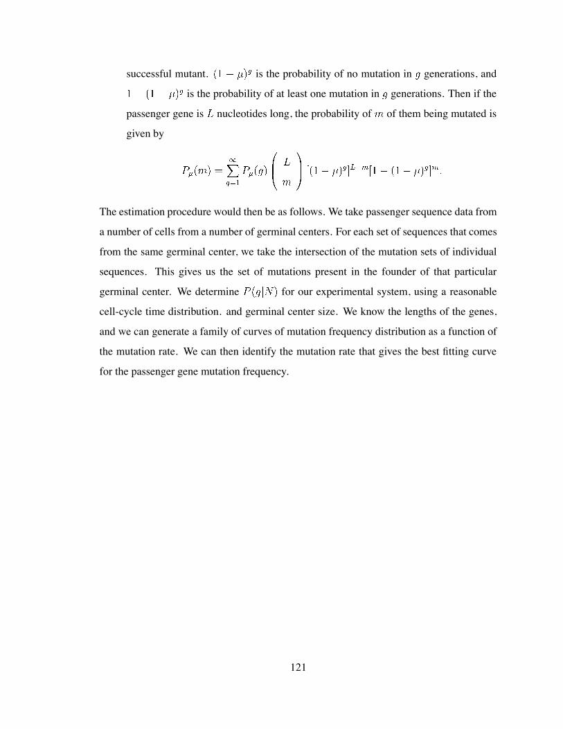
successful mutant. is the probability of no mutation in generations, and

is the probability of at least one mutation in generations. Then if the

passenger gene is nucleotides long, the probability of of them being mutated is

given by

The estimation procedure would then be as follows. We take passenger sequence data from

a number of cells from a number of germinal centers. For each set of sequences that comes

from the same germinal center, we take the intersection of the mutation sets of individual

sequences. This gives us the set of mutations present in the founder of that particular

germinal center. We determine for our experimental system, using a reasonable

cell-cycle time distribution. and germinal center size. We know the lengths of the genes,

and we can generate a family of curves of mutation frequency distribution as a function of

the mutation rate. We can then identify the mutation rate that gives the best fitting curve

for the passenger gene mutation frequency.

121

Chapter 7

Conclusions

I would like now to review the questions that I addressed in my dissertation and summarize

what I learned from the experiments that I constructed.

The immune system is viewed as a detection system. It detects pathogenic intru-

sions. In contrast to the familiar detection systems though, the immune system can recog-

nize pathogens that the organism may have never encountered before in its life time. This

ability derives, to a certain extent, from the generality of the language of biochemistry. A

variety of immune receptors are generated without regard to what they may be binding.

Those that react strongly with molecules that are normally present in the body are weeded

out, and those that remain will, by definition, recognize ”outsider” molecules. However,

the immune system has only a limited number of cells that circulate at any time through the

body. It is therefore crucial that the immune system makes optimal use of its resources by

placing the receptors “strategically” in the space of all possible receptors. Having the right

type of lymphocytes in the right number is crucial for the survival of the organism.

The questions that I addressed in my thesis are related to how the immune system

might learn to anticipate its pathogenic environment. Based on the results that I summarize

below, I argue that:

The recognition capacity of the immune system is targeted to pathogens that it has

encountered during evolution. It does not attempt to recognize as many molecular

122

shapes as possible.

Germline diversity does not contribute to the direct, specific recognition of pathogens,

but rather realizes a coarse-grained coverage of the pathogen space.

Immune receptor diversification during an on-going immune response is the deter-

minant factor for the specificity and affinity of the antibodies. If the immune system

fails to recognize a pathogen with high affinity, it means that:

– the pathogen mimics the self structures too closely, or

– the pathogen is an emergent pathogen, considerably different from those that

the immune system has seen during its recent evolution, or

– somatic hypermutation fails to produce a high affinity antibody for that pathogen,

due probably to sequence peculiarities of the germline-encoded antibody that

underwent somatic hypermutation.

My detailed results also bear on the construction of random antibody libraries, as well as on

computational methods that may be used for mutational analysis in a variety of biological

systems.

Note that I did not consider the effect of junctional diversity on the repertoire. The

reasons are as follows:

I focused on the aspects of evolutionary learning in the immune system. The rear-

rangement process is essentially thought to produce ”random” junctions. It could

thus not be the substrate for learning.

If the rearrangement process indeed produces ”random” junctions, then its contribu-

tion to the repertoire is to increase the size of the primary repertoire. However, if this

repertoire cannot cover pathogens individually, then the results that I presented based

on a single library are expected to hold.

123

7.1 Summary of results

7.1.1 Germline diversity does not contribute to the direct recognition

of pathogens

In chapter 2 I used a simple model of gene library evolution to investigate the scaling of

the survival probability of an organism with the number of antibodies in its repertoire.

I showed that for distributions of the antibody-antigen bond strength that I consider of

biological relevance, the survival probability of the organism increases logarithmically, or

sublogarithmically, with the size of its germline-encoded antibody repertoire. This suggests

that the role of germline-encoded immune receptor genes is not specific recognition of

individual pathogens, but rather a coarse-grain encoding of the region of the pathogen

universe that the species has encountered in evolution. I showed that such an encoding can

be achieved if an individual is confronted with a large fraction of the possible pathogens

in its life time. High-affinity recognition of a pathogen would then have to be achieved

through fine-tuning of the antigen receptor during an immune response. If the number of

pathogens that the organism encounters is comparable with the number of receptors that it

can encode in germline, then a static pathogenic environment would result in better learning

of the training set. However, if the pathogenic environment changes, the performance of

the immune system would be lower on the pathogens that it encountered, but it would

be higher on random pathogens. The reason for this behavior, which one might view as

robustness, is that, although static pathogenic environments result in specialized libraries,

dynamic pathogenic environments induce essentially random antibody libraries.

7.1.2 Immunoglobulin genes evolved plasticity for somatic hypermu-

tation

The basic mechanism that is responsible for fine-tuning of antigen receptors has been de-

scribed. It is termed affinity maturation, and it involves rounds of essentially random mu-

124

tagenesis followed by selection. In chapter 3, I introduced a new method for analyzing the

plasticity of individual immunoglobulin genes under somatic hypermutation. I showed that

codon bias consistent with low framework, and high complementarity-determining region,

mutability is found in individual region genes in a variety of species. I also showed that

the codon composition of the genes is a good predictor of their mutability. The methods that

I introduced in this chapter can be applied both to the analysis of individual gene sequences,

as well to sets of genes. These are both important issues. In somatic hypermutation experi-

ments there is always the question of the intrinsic mutability of the gene relative to selection

pressures that operate on the protein product. Also, the study of the immunoglobulin gene

family is generally difficult due to the close genealogical relationship between these genes.

These problems are explicitly addressed in the tests that I designed. I further analyzed

the sequence specificity of the somatic hypermutation mechanism by applying it to a set

of non-immunoglobulin genes. Intriguingly, I found that these genes have a codon bias

consistent with low mutability under somatic hypermutation as well. This result suggests

a possible connection between the somatic hypermutation mechanism and more general

processes that operate throughout the genome. I provided further supporting evidence, by

showing that the somatic hypermutation mechanism reveals the A/T content of the gene.

That the evolutionary stability of A/T-rich nucleic acids, and the proteins they encode, is

lower than their G/C-rich counterparts has already been shown, though the factors that may

be responsible for it are debated.

7.1.3 The efficiency of affinity maturation can only be explained by

multiple rounds of mutation-selection-expansion of lymphocytes

The germinal center reaction is generally described as a one-pass process, with B cells

coming into the germinal center, undergoing division and somatic mutation in one compart-

ment, then moving into another compartment for selection, and finally leaving the germinal

center. There have been a number of studies showing that a large number of high affinity

mutants can be produced more efficiently if cells were to cycle between the selection com-

125

partment and the reproduction compartment. In chapter 5 I showed quantitatively that the

one-pass scenario is incompatible with the observed efficiency of affinity maturation. I also

showed that the decay of the selective agent (antigen) reduces the efficiency of amplifica-

tion of high-affinity cells from linear to logarithmic in their selective advantage. This gives

even more theoretical support to the recycling hypothesis. It also provides useful insights

into processes in which selection is due to an agent that decays in time.

7.1.4 Improved methods for mutation rate estimation

In trying to understand the mechanism responsible for somatic hypermutation, one often

encounters the problem of accurately estimating the mutation rate. The currently employed

method is based on the fluctuation analysis experiment of Luria and Delbruck (1943).

While attempting to adapt this method to mutation rate estimation in germinal centers, I

found that, due to implicit assumptions about the cell-cycle time distribution, this method

underestimates the mutation rate by as much as 30%. In chapter 6, I introduced a number of

methods for estimating mutation rates and constructing confidence intervals, each of which

takes into consideration the cell-cycle time distribution. I gave cell-cycle corrections for the

mean proportion of mutants in the culture for two of the most common models of cell cycle

time. The derivation can be used for other cell cycle time distributions as well. I described

a continuum approximation for the Luria-Delbruck distribution, that is considerably easier

to use than the currently available methods. I also give a parametrization of this distribu-

tion that can be used for cell cultures of arbitrary size, provided that the cell cycle time

obeys a shifted exponential distribution. Gamma-distributed cell cycle times do not allow

a similar parametrization of cLD. However, I found that the 5% and 95% of the proportion

of mutants scale linearly with the mutation rate. Moreover, the slope of these curves does

not seem to be sensitive to the culture size. These findings allowed me to design a method

for constructing confidence intervals for the mutation rate in this types of cell cultures as

well. Finally, I discuss extensions of the above methods for cultures that reach steady-state,

as well as for germinal centers. Given that they readily lend themselves to automatization,

126

I believe that the methods that I introduced in this chapter have the potential of becoming

widely adopted in the field of experimental biology.

7.2 Future work

I think I have reached an understanding of the role of germline diversity and somatic mu-

tation in generating the immune repertoire. However, there still are a number of related

problems that I am currently working on, or hope to be working on in the near future.

The most concrete project concerns implementing the mutation rate estimation methods

that I only introduced conceptually in my dissertation. There are other issues that could

be pursued, based on the work that I presented here. We parametrized the Luria-Delbruck

distribution using a parameter that we determined empirically, by fitting to simulation data.

We do not have an analytical form for this parameter. It would be of great interest to find

that form. Moreover, for the case of gamma-distributed cell cycle times, we do not have as

much as a distribution based on an empirically-determined parameter.

The finding that non-immunoglobulin sequences share optimization features with

respect to somatic hypermutation raises the exciting possibility that somatic hypermutation

is derived from more general mutation mechanisms that operate across the genome. What

the nature of these mechanisms might be has not been revealed by my analyses. I have,

however, a starting point for that search. That is the observation that somatic mutation

targets A/T nucleotides. The next step is to look into what mutation/repair mechanisms

might share such a bias. One candidate is the single-base mismatch repair that seem to

preserve G nucleotides (Bill et al., 1998). I also intend to determine the sequence specificity

of the germline mutation mechanism and compare it directly to the specificity of somatic

hypermutation.

In my analysis of the properties of the germline-encoded repertoire, I concluded that

”sticky” antibodies are a good anticipative strategy. Antibodies of this type indeed have

been described, especially in neonatal immune systems. However, they pose the problem

127

that they bind not only pathogens, but also self structures. We could now introduce a set

of self molecules and require that the repertoire not bind these molecules. It would be very

interesting to find out what type of antibodies would emerge under these conditions.

Finally, there are processes which take place at the gene level, that might constrain

the learning capacity of the immune system. These have not been not been taken into

account by the models that I described in this dissertation. They are, however, important

issues to consider if one is to understand the dynamics of the immune repertoire. The

generation of the antibody repertoire in neonates seems to be much more deterministic

than in adults. This justified, in part, my analysis of the ”germline-encoded” antibodies.

These antibodies are characterized by the lack of non-templated nucleotide additions, and

by preferential V-D, D-J, and V-J associations. It is believed that short regions of homology

at the ends of the rearranging fragments are responsible for constraining the rearrangement

process. I intend to build a mechanistic model for the rearrangement process, which I can

use to test the previous hypothesis.

Gene conversion introduces a sampling dynamics at the level of genes. It would be

interesting to know how much germline diversity can be maintained with reasonable values

of the parameters that determine the dynamics of gene conversion. In certain species, such

as chicken and rabbit, gene conversion is used as a primary diversification mechanism, re-

sponsible for creating the naive repertoire. The donor genes are generally pseudo-genes,

that is they cannot, by themselves, generate functional immunoglobulins. It would be in-

teresting to know what type of dynamics these genes have, given that they are constrained

by the interaction with the acceptor gene. The mechanism of gene conversion is also not

known. Using gene conversion data, one could attempt to infer what this mechanism might

be, in a way that would be similar to my attempt to infer the nature of the somatic hyper-

mutation mechanism.

128

7.3 In lieu of closing

As can be inferred from the previous section, the topics that I explored in my dissertation

are far from being exhausted. In fact, it seems that I have only managed to scratch the

surface. Or, the way I think about it, to set the stage for a more rigurous understanding of

these processes. As of what I will be remembered by...

129

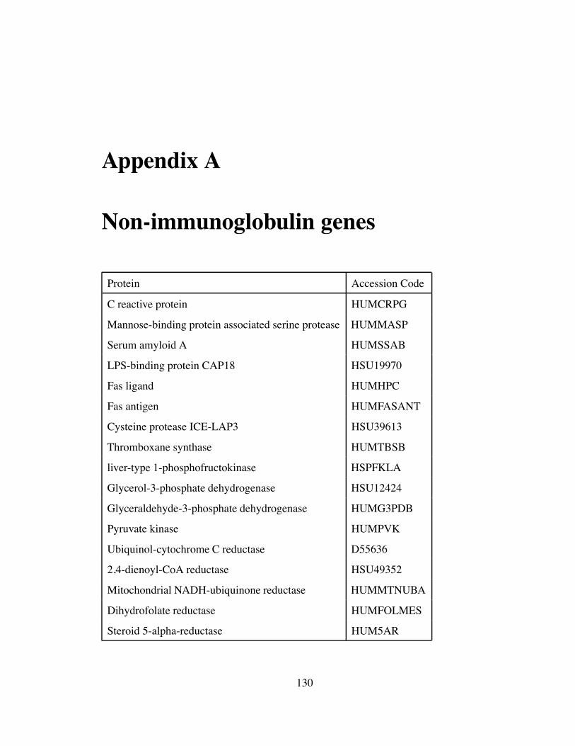
Appendix A

Non-immunoglobulin genes

Protein Accession Code

C reactive protein HUMCRPG

Mannose-binding protein associated serine protease HUMMASP

Serum amyloid A HUMSSAB

LPS-binding protein CAP18 HSU19970

Fas ligand HUMHPC

Fas antigen HUMFASANT

Cysteine protease ICE-LAP3 HSU39613

Thromboxane synthase HUMTBSB

liver-type 1-phosphofructokinase HSPFKLA

Glycerol-3-phosphate dehydrogenase HSU12424

Glyceraldehyde-3-phosphate dehydrogenase HUMG3PDB

Pyruvate kinase HUMPVK

Ubiquinol-cytochrome C reductase D55636

2,4-dienoyl-CoA reductase HSU49352

Mitochondrial NADH-ubiquinone reductase HUMMTNUBA

Dihydrofolate reductase HUMFOLMES

Steroid 5-alpha-reductase HUM5AR

130

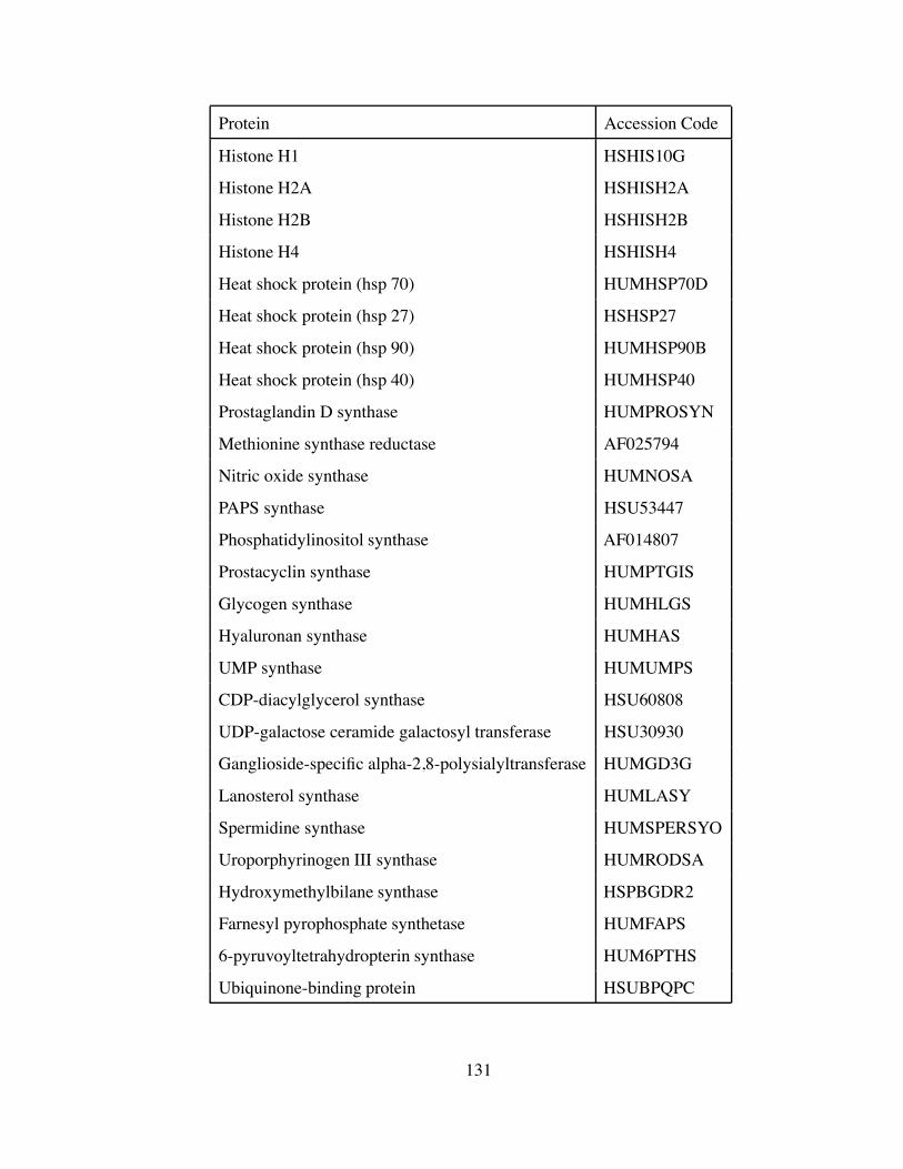
Protein Accession Code

Histone H1 HSHIS10G

Histone H2A HSHISH2A

Histone H2B HSHISH2B

Histone H4 HSHISH4

Heat shock protein (hsp 70) HUMHSP70D

Heat shock protein (hsp 27) HSHSP27

Heat shock protein (hsp 90) HUMHSP90B

Heat shock protein (hsp 40) HUMHSP40

Prostaglandin D synthase HUMPROSYN

Methionine synthase reductase AF025794

Nitric oxide synthase HUMNOSA

PAPS synthase HSU53447

Phosphatidylinositol synthase AF014807

Prostacyclin synthase HUMPTGIS

Glycogen synthase HUMHLGS

Hyaluronan synthase HUMHAS

UMP synthase HUMUMPS

CDP-diacylglycerol synthase HSU60808

UDP-galactose ceramide galactosyl transferase HSU30930

Ganglioside-specific alpha-2,8-polysialyltransferase HUMGD3G

Lanosterol synthase HUMLASY

Spermidine synthase HUMSPERSYO

Uroporphyrinogen III synthase HUMRODSA

Hydroxymethylbilane synthase HSPBGDR2

Farnesyl pyrophosphate synthetase HUMFAPS

6-pyruvoyltetrahydropterin synthase HUM6PTHS

Ubiquinone-binding protein HSUBPQPC

131

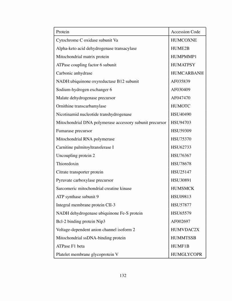
Protein Accession Code

Cytochrome C oxidase subunit Va HUMCOXNE

Alpha-keto acid dehydrogenase transacylase HUME2B

Mitochondrial matrix protein HUMPMMP1

ATPase coupling factor 6 subunit HUMATPSY

Carbonic anhydrase HUMCARBANH

NADH:ubiquinone oxyreductase B12 subunit AF035839

Sodium-hydrogen exchanger 6 AF030409

Malate dehydrogenase precursor AF047470

Ornithine transcarbamylase HUMOTC

Nicotinamid nucleotide transhydrogenase HSU40490

Mitochondrial DNA polymerase accessory subunit precursor HSU94703

Fumarase precursor HSU59309

Mitochondrial RNA polymerase HSU75370

Carnitine palmitoyltransferase I HSU62733

Uncoupling protein 2 HSU76367

Thioredoxin HSU78678

Citrate transporter protein HSU25147

Pyruvate carboxylase precursor HSU30891

Sarcomeric mitochondrial creatine kinase HUMSMCK

ATP synthase subunit 9 HSU09813

Integral membrane protein CII-3 HSU57877

NADH dehydrogenase ubiquinone Fe-S protein HSU65579

Bcl-2 binding protein Nip3 AF002697

Voltage-dependent anion channel isoform 2 HUMVDAC2X

Mitochondrial ssDNA-binding protein HUMMTSSB

ATPase F1 beta HUMF1B

Platelet membrane glycoprotein V HUMGLYCOPR

132

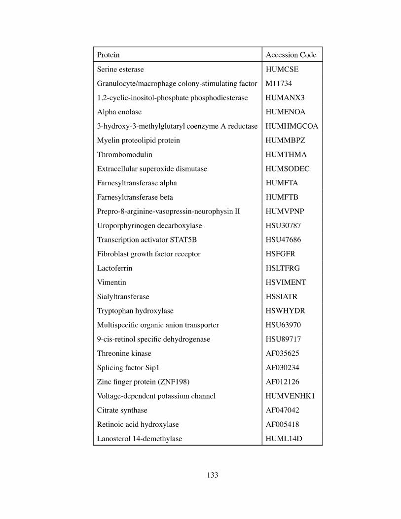
Protein Accession Code

Serine esterase HUMCSE

Granulocyte/macrophage colony-stimulating factor M11734

1,2-cyclic-inositol-phosphate phosphodiesterase HUMANX3

Alpha enolase HUMENOA

3-hydroxy-3-methylglutaryl coenzyme A reductase HUMHMGCOA

Myelin proteolipid protein HUMMBPZ

Thrombomodulin HUMTHMA

Extracellular superoxide dismutase HUMSODEC

Farnesyltransferase alpha HUMFTA

Farnesyltransferase beta HUMFTB

Prepro-8-arginine-vasopressin-neurophysin II HUMVPNP

Uroporphyrinogen decarboxylase HSU30787

Transcription activator STAT5B HSU47686

Fibroblast growth factor receptor HSFGFR

Lactoferrin HSLTFRG

Vimentin HSVIMENT

Sialyltransferase HSSIATR

Tryptophan hydroxylase HSWHYDR

Multispecific organic anion transporter HSU63970

9-cis-retinol specific dehydrogenase HSU89717

Threonine kinase AF035625

Splicing factor Sip1 AF030234

Zinc finger protein (ZNF198) AF012126

Voltage-dependent potassium channel HUMVENHK1

Citrate synthase AF047042

Retinoic acid hydroxylase AF005418

Lanosterol 14-demethylase HUML14D

133

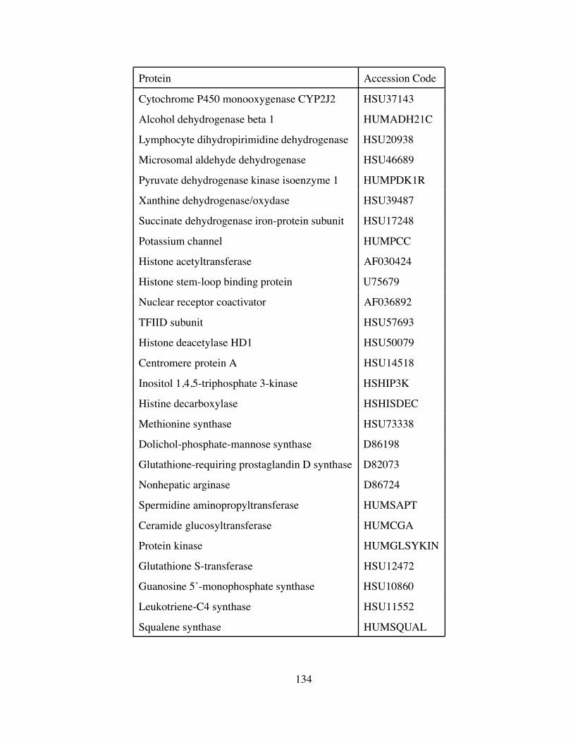
Protein Accession Code

Cytochrome P450 monooxygenase CYP2J2 HSU37143

Alcohol dehydrogenase beta 1 HUMADH21C

Lymphocyte dihydropirimidine dehydrogenase HSU20938

Microsomal aldehyde dehydrogenase HSU46689

Pyruvate dehydrogenase kinase isoenzyme 1 HUMPDK1R

Xanthine dehydrogenase/oxydase HSU39487

Succinate dehydrogenase iron-protein subunit HSU17248

Potassium channel HUMPCC

Histone acetyltransferase AF030424

Histone stem-loop binding protein U75679

Nuclear receptor coactivator AF036892

TFIID subunit HSU57693

Histone deacetylase HD1 HSU50079

Centromere protein A HSU14518

Inositol 1,4,5-triphosphate 3-kinase HSHIP3K

Histine decarboxylase HSHISDEC

Methionine synthase HSU73338

Dolichol-phosphate-mannose synthase D86198

Glutathione-requiring prostaglandin D synthase D82073

Nonhepatic arginase D86724

Spermidine aminopropyltransferase HUMSAPT

Ceramide glucosyltransferase HUMCGA

Protein kinase HUMGLSYKIN

Glutathione S-transferase HSU12472

Guanosine 5’-monophosphate synthase HSU10860

Leukotriene-C4 synthase HSU11552

Squalene synthase HUMSQUAL

134

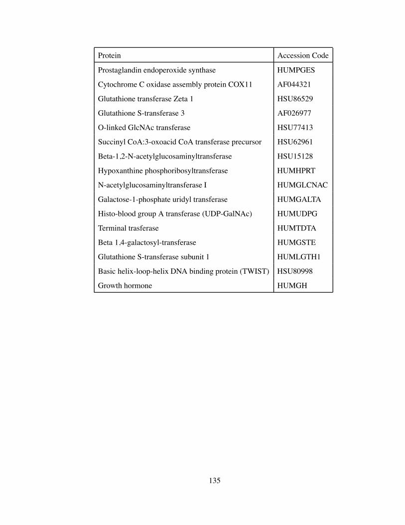
Protein Accession Code

Prostaglandin endoperoxide synthase HUMPGES

Cytochrome C oxidase assembly protein COX11 AF044321

Glutathione transferase Zeta 1 HSU86529

Glutathione S-transferase 3 AF026977

O-linked GlcNAc transferase HSU77413

Succinyl CoA:3-oxoacid CoA transferase precursor HSU62961

Beta-1,2-N-acetylglucosaminyltransferase HSU15128

Hypoxanthine phosphoribosyltransferase HUMHPRT

N-acetylglucosaminyltransferase I HUMGLCNAC

Galactose-1-phosphate uridyl transferase HUMGALTA

Histo-blood group A transferase (UDP-GalNAc) HUMUDPG

Terminal trasferase HUMTDTA

Beta 1,4-galactosyl-transferase HUMGSTE

Glutathione S-transferase subunit 1 HUMLGTH1

Basic helix-loop-helix DNA binding protein (TWIST) HSU80998

Growth hormone HUMGH

135

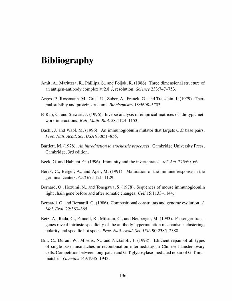
Bibliography

Amit, A., Mariuzza, R., Phillips, S., and Poljak, R. (1986). Three dimensional structure ofan antigen-antibody complex at 2.8 ˚ resolution. Science 233:747–753.

Argos, P., Rossmann, M., Grau, U., Zuber, A., Franck, G., and Tratschin, J. (1979). Ther-mal stability and protein structure. Biochemistry 18:5698–5703.

B-Rao, C. and Stewart, J. (1996). Inverse analysis of empirical matrices of idiotypic net-work interactions. Bull. Math. Biol. 58:1123–1153.

Bachl, J. and Wabl, M. (1996). An immunoglobulin mutator that targets G.C base pairs.Proc. Natl. Acad. Sci. USA 93:851–855.

Bartlett, M. (1978). An introduction to stochastic processes. Cambridge University Press,Cambridge, 3rd edition.

Beck, G. and Habicht, G. (1996). Immunity and the invertebrates. Sci. Am. 275:60–66.

Berek, C., Berger, A., and Apel, M. (1991). Maturation of the immune response in thegerminal centers. Cell 67:1121–1129.

Bernard, O., Hozumi, N., and Tonegawa, S. (1978). Sequences of mouse immunoglobulinlight chain gene before and after somatic changes. Cell 15:1133–1144.

Bernardi, G. and Bernardi, G. (1986). Compositional constraints and genome evolution. J.Mol. Evol. 22:363–365.

Betz, A., Rada, C., Pannell, R., Milstein, C., and Neuberger, M. (1993). Passenger trans-genes reveal intrinsic specificity of the antibody hypermutation mechanism: clustering,polarity and specific hot spots. Proc. Natl. Acad. Sci. USA 90:2385–2388.

Bill, C., Duran, W., Miselis, N., and Nickoloff, J. (1998). Efficient repair of all typesof single-base mismatches in recombination intermediates in Chinese hamster ovarycells. Competition between long-patch and G-T glycosylase-mediated repair of G-T mis-matches. Genetics 149:1935–1943.

136

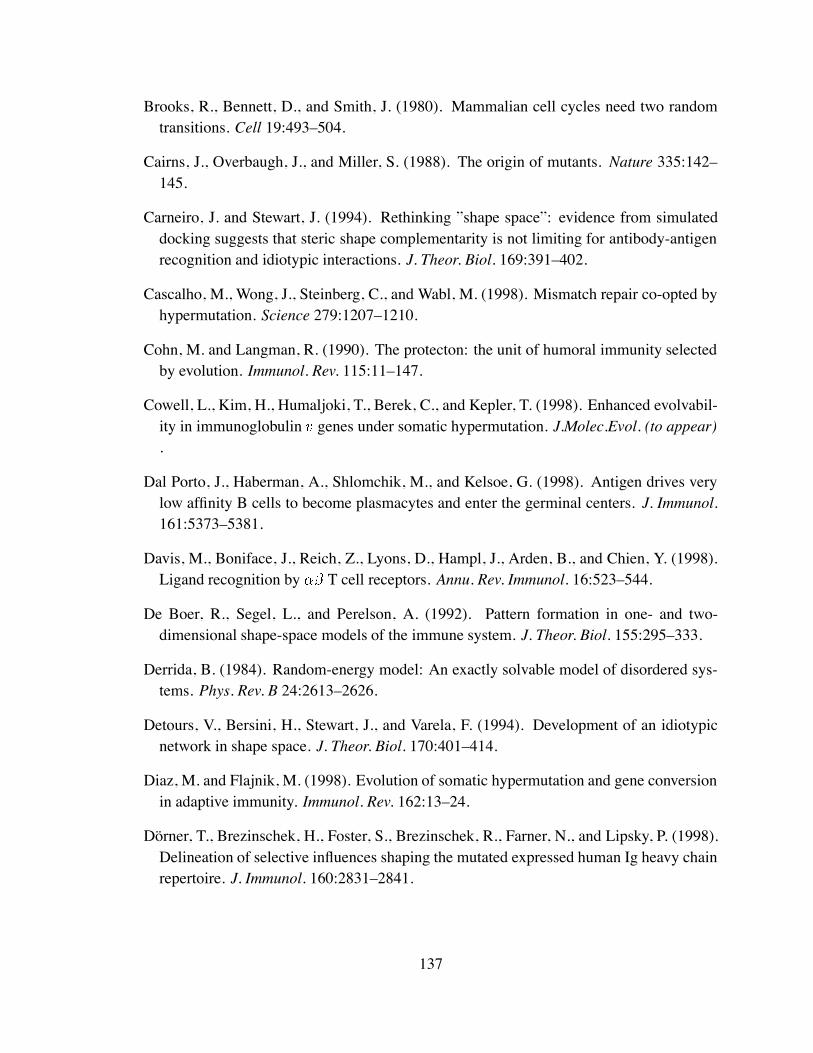
Brooks, R., Bennett, D., and Smith, J. (1980). Mammalian cell cycles need two randomtransitions. Cell 19:493–504.

Cairns, J., Overbaugh, J., and Miller, S. (1988). The origin of mutants. Nature 335:142–145.

Carneiro, J. and Stewart, J. (1994). Rethinking ”shape space”: evidence from simulateddocking suggests that steric shape complementarity is not limiting for antibody-antigenrecognition and idiotypic interactions. J. Theor. Biol. 169:391–402.

Cascalho, M., Wong, J., Steinberg, C., and Wabl, M. (1998). Mismatch repair co-opted byhypermutation. Science 279:1207–1210.

Cohn, M. and Langman, R. (1990). The protecton: the unit of humoral immunity selectedby evolution. Immunol. Rev. 115:11–147.

Cowell, L., Kim, H., Humaljoki, T., Berek, C., and Kepler, T. (1998). Enhanced evolvabil-ity in immunoglobulin genes under somatic hypermutation. J.Molec.Evol. (to appear).

Dal Porto, J., Haberman, A., Shlomchik, M., and Kelsoe, G. (1998). Antigen drives verylow affinity B cells to become plasmacytes and enter the germinal centers. J. Immunol.161:5373–5381.

Davis, M., Boniface, J., Reich, Z., Lyons, D., Hampl, J., Arden, B., and Chien, Y. (1998).Ligand recognition by T cell receptors. Annu. Rev. Immunol. 16:523–544.

De Boer, R., Segel, L., and Perelson, A. (1992). Pattern formation in one- and two-dimensional shape-space models of the immune system. J. Theor. Biol. 155:295–333.

Derrida, B. (1984). Random-energy model: An exactly solvable model of disordered sys-tems. Phys. Rev. B 24:2613–2626.

Detours, V., Bersini, H., Stewart, J., and Varela, F. (1994). Development of an idiotypicnetwork in shape space. J. Theor. Biol. 170:401–414.

Diaz, M. and Flajnik, M. (1998). Evolution of somatic hypermutation and gene conversionin adaptive immunity. Immunol. Rev. 162:13–24.

Dorner, T., Brezinschek, H., Foster, S., Brezinschek, R., Farner, N., and Lipsky, P. (1998).Delineation of selective influences shaping the mutated expressed human Ig heavy chainrepertoire. J. Immunol. 160:2831–2841.

137

Dorner, T., Brezinschek, H.-P., Foster, S., Domiati Saad, R., and Lipsky, P. (1997). Anal-ysis of the frequency pattern of somatic mutations within nonproductively rearrangedhuman variable heavy chain genes. J. Immunol. 158:2779–2789.

Dunn-Walters, D., Dogan, A., Boursier, L., MacDonald, C., and Spencer, J. (1998). Base-specific sequences that bias somatic hypermutation deduced by analysis of out-of-framehuman IgVH genes. J. Immunol. 160:2360–2364.

Feeney, A. (1992). Predominance of junctions occuring at sites of shortsequence homology results in limited junctional diversity in neonatal antibodies. J. Im-munol. 149:222–229.

Fisher, R. (1930). The genetical theory of natural selection. Oxford University Press.

Foote, J. and Winter, G. (1992). Antibody framework residues affecting the conformationof the hypervariable loops. J. Mol. Biol. 224:487–499.

Frey, S., Bertocci, B., Delbos, F., Quint, L., Weill, J.-C., and Raynaud, C.-A. (1998).Mismatch repair deficiency interferes with the accumulation of mutations in chronicallystimulated B cells and not with the hypermutation process. Immunity 9:127–134.

Gilfillan, S., Bachmann, M., Trembleau, S., Adorini, L., Kalinke, U., Zinkernagel, R.,Benoist, C., and Mathis, D. (1995). Efficient immune responses in mice lacking N-region diversity. Eur. J. Immunol. 25:3115–3122.

Gilfillan, S., Dierich, A., Lemeur, M., Benoist, C., and Mathis, D. (1993). Mice lackingTdT: mature animals with an immature lymphocyte repertoire. Science 261:1175–1178.

Giudicelli, V., Chaume, D., Bodmer, J., Muller, W., Busin, C., Marsh, S., Bontrop, R.,Marc, L., Malik, A., and M.P., L. (1997). IMGT, the international ImMunoGeneTicsdatabase. Nucleic Acids Res. 25:206–211.

Goodlad, J. and Macartney, J. (1995). Regulation of murine germinal centre cell prolifer-ation in vivo: A stathmokinetic study examining the effect of differently timed doses ofcyclosporin A. J. Pathol. 176:87–97.

Hanna, M. (1964). An autoradiographic study of the germinal center in spleen white pulpduring early intervals of the immune response. Lab. Invest. 13:95–104.

Higgins, D. and Sharp, P. (1988). CLUSTAL: a package for performing multiple sequencealignments on a microcomputer. Gene 73:237–244.

Hightower, R. (1996). Computational aspect of antibody gene families. Ph.D. thesis,University of New Mexico.

138

Hinds-Frey, K., Nishikata, H., Litman, R., and Litman, G. (1993). Somatic variation pre-ceeds extensive diversification of germline sequences and combinatorial joining in theevolution of immunoglobulin heavy chain diversity. J. Exp. Med. 178:815–824.

Hsu, E. (1998). Mutation, selection, and memory in b lymphocytes of exothermic verte-brates. Immunol. Rev. 162:25–36.

Huisman, G., Siegele, D., Zambrano, M., and Kolter, R. (1996). Morphological and phys-iological changes during stationary phase. In Escherichia coli and Salmonella, F. Neid-hardt, ed., pp. 1672–1682. ASM Press, Washington, D.C.

Ikemura, T. (1981). Correlation between the abundance of Escherichia coli transfer RNAsand the occurence of the respective codons in its protein genes: a proposal for a syn-onymous codon choice that is optimal for the E. coli translational system. J. Mol. Evol.151:389–409.

Ikemura, T. (1985). Codon usage and tRNA content in unicellular and multicellular organ-isms. Mol. Biol. Evol. 2:13–34.

Insel, R., Adderson, E., and Carroll, W. (1992). The repertoire of human antibody to theHaemophilus influenzae type b capsular polysaccharide. Int. Rev. Immunol. 9:25–42.

Insel, R. and Varade, W. (1998). Characteristics of somatic hypermutation of human im-munoglobulin genes. Curr. Top. Microbiol. Immunol. 229:33–44.

Jacob, J., Kassir, R., and Kelsoe, G. (1991). In situ studies of the primary immune responseto (4-hydroxy-3-nitrophenyl)acetyl. I. The architecture and dynamics of responding cellpopulations. J. Exp. Med. 173:1165–1175.

Jacob, J. and Kelsoe, G. (1992). In situ studies of the primary immune response to (4-hydroxy-3-nitrophenyl)acetyl. II. A common clonal origin for periarteriolar lymphoidsheath-associated foci and germinal centers. J. Exp. Med. 176:679–687.

Jones, M., Thomas, S., and Rogers, A. (1994). Luria-Delbruck fluctuation experiments:design and analysis. Genetics 136:1209–1216.

Kearney, J., Bartels, J., Hamilton, A., Lehuen, A., Solvason, N., and Vakil, M. (1992).Development and function of the early B cell repertoire. Intern. Rev. Immunol. 8:247–257.

Kelly, C. and Rahn, O. (1932). The growth of individual bacterial cells. J. Bacteriol.23:147–153.

139

Kelsoe, G. (1998). V(D)J hypermutation and DNA mismatch repair: Vexed by fixation.Proc. Natl. Acad. Sci. USA 95:6576–6577.

Kendall, D. (1948). On the role of variable generation time in the development of a stochas-tic birth process. Biometrika 35:316–330.

Kendall, D. (1952). Les procesus stochastiques de croissance in biologie. Ann. Inst. H.Poincare 13:43–108.

Kepler, T. (1997). Codon bias and plasticity in immunoglobulins. Mol. Biol. Evol. 14:637–643.

Kepler, T. and Bartl, S. (1998). Plasticity under somatic mutation in antigen receptors.Curr. Top. Microbiol. Immunol. 229:149–162.

Kepler, T. and Perelson, A. (1993). Cyclic re-entry of germinal center B cells and theefficiency of affinity maturation. Immunol.Today 14:412–415.

Knuth, D. (1973). The art of computer programming, vol. 2. Addison-Wesley PublishingCompany, Inc.

Kroese, F., Wubenna, A., Seijen, H., and Nieuwenhuis, P. (1987). Germinal centers developoligoclonally. Eur. J. Immunol. 17:1069–1072.

Langman, R. and Cohn, M. (1993). Two signal models of lymphocyte activation? Immunol.Today 14:235–237.

Lea, D. and Coulson, C. (1949). The distribution of the number of mutants in bacterialpopulations. J. Genetics 49:264–284.

Lebecque, S. and Gearhart, P. (1990). Boundaries of somatic mutation in rearranged im-munoglobulin genes: 5’ boundary is near the promoter, and 3’ boundary is approximately1 kb from V(D)J gene. J. Exp. Med. 172:1717–1727.

Lee, W., Cosenza, H., and Kohler, H. (1974). Clonal restriction of the immune response tophosphorylcholine. Nature 247:55–61.

Li, W.-H. (1997). Molecular evolution. Sinauer Associates, Inc. Sunderland Massachusetts01375 USA.

Liu, Y. J., Zhang, J., Lane, P. J. L., Chan, E. Y.-T., and MacLennan, I. C. M. (1991). Sitesof specific B cell activation in primary and secondary responses to T cell-dependent andT cell-independent antigens. Eur. J. Immunol. 21:2951–2962.

140

Luria, S. and Delbruck, M. (1943). Mutations of bacteria from virus sensitivity to virusresistance. Genetics 28:491–511.

MacLennan, I. (1991). The centre of hypermutation. Nature 354:352–353.

MacLennan, I. C. M. (1994). Germinal centers. Annu. Rev. Immunol. 12:117–139.

MacLennan, I. C. M., Liu, Y. J., Olfield, S., Zhang, J., and Lane, P. J. L. (1990). Theevolution of B-cell clones. Curr. Top. Microbiol. Immunol. 159:37–63.

MacWilliams, F. and Sloane, N. (1986). The theory of error correcting codes. ElsevierScience Publishers, B.V.

Matzinger, P. (1994). Tolerance, danger and the extended family. Annu. Rev. Immunol.12:991–1045.

McKean, D. M., Huppi, K., Bell, M., Staudt, L., Gerhard, W., and Weigert, M. (1984).Generation of antibody diversity in the immune response of BALB/c mice to influenzavirus hemagglutinin. Proc. Natl. Acad. Sci. USA 81:3180–3184.

Milstein, C., Neuberger, M., and Staden, R. (1998). Both DNA strands of antibody genesare hypermutation targets. Proc. Natl. Acad. Sci. USA 95:8791–8794.

Minar, N. (1994). Suboptimal solutions in a simple GA problem and the underuse ofgenetic material (unpublished manuscript). http://www.santafe.edu/nelson/gaimmune .

Mitchell, M. (1996). An introduction to genetic algorithms. The MIT Press, Cambridge,Massachusetts.

Motoyama, N., Okada, H., and Azuma, T. (1991). Somatic mutation in constant regions ofmouse light chains. Proc. Natl. Acad. Sci. USA 88:7933–7937.

Nossal, G. (1971). Antibodies and immunity. Pelican Books, Ltd., Harmondsworth, Mid-dlesex, England.

Nossal, G. (1992). The molecular and cellular basis of affinity maturation in the antibodyresponse. Cell 68:1–2.

Oprea, M. and Perelson, A. (1997). Somatic mutation leads to efficient affinity maturationwhen centrocytes recycle back to centroblasts. J. Immunol. 158:5155–5162.

Perelson, A. (1989). Immune network theory. Immunol. Rev. 110:5–36.

Perelson, A. and Oster, G. (1979). Theoretical studies of clonal selection: minimal antibodyrepertoire size and reliability of self-non-self discrimination. J. Theor. Biol. 81:645–670.

141

Phung, Q., Winter, D., Cranston, A., Tarone, R., Bohr, V., Fishel, R., and Gearhart, P.(1998). Increased hypermutation at G and C nucleotides in immunoglobulin variablegenes from mice deficient in the MSH2 mismatch repair protein. J. Exp. Med. 187:1745–1751.

Press, W., Flannery, B., Teukolsky, S., and Vetterling, W. (1988). Numerical recipes in C.Cambridge University Press, Cambridge.

Radmacher, M., Kelsoe, G., and Kepler, T. (1998). Predicted and inferred waiting times forkey mutations in the germinal center reaction: Evidence for stochasticity in selection.Immunol. Cell Biol. 76:373–381.

Reynaud, C., Garcia, C., and J.C., W. (1995). Hypermutation generating the sheep im-munoglobulin repertoire is an antigen-independent process. Cell 80:115–125.

Rogozin, I. and Kolchanov, N. (1992). Somatic hypermutagenesis in immunoglobulingenes. II. Influence of neighboring base sequences on mutagenesis. Biochim. Biophys.Acta 1171:11–18.

Roux, K., Greenberg, A. S., Greene, L., Strelets, L., Avila, D., McKinney, E., and Flajnik,M. (1998). Structural analysis of the nurse shark (new) antigen receptor (NAR): Molec-ular convergence of NAR and unusual mammalian immunoglobulins. Proc. Natl. Acad.Sci. USA 95:11804–11809.

Sarkar, S. A. (1992). On fluctuation analysis: a new, simple and efficient method forcomputing the expected number of mutants. Genetica 85:173–179.

Segel, L. and Perelson, A. (1989). Shape space: an approach to the evaluation of cross-reactivity effects, stability and controllability in the immune system. Immunol. Lett.22:91–99.

Seidman, J., Leder, A., Edgell, M., Polsky, F., Tilghman, S., Tiemeier, D., and Leder, P.(1978). Multiple related immunoglobulin variable region genes identified by cloning andsequence analysis. Proc. Natl. Acad. Sci. USA 75:3881–3885.

Smith, D., Creadon, G., Jena, P., Portanova, J., Kotzin, B., and Wysocki, L. (1996). Di-and trinucleotide target preferences in somatic mutagenesis in normal and autoreactiveB cells. J. Imunol. 156:2642–2652.

Smith, D., Forrest, S., Hightower, R., and Perelson, A. (1997). Deriving shape spaceparameters from immunological data. J. Theor. Biol. 189:141–150.

Smith, J. and Martin, L. (1973). Do cells cycle? Proc. Natl. Acad. Sci. USA 70:1263–1267.

142

Stewart, F., Gordon, D., and Levin, B. (1990). Fluctuation analysis: the probability distri-bution of the number of mutants under different conditions. Genetics 124:175–185.

Van der Stoep, N., Van der Linden, J., and Logtenberg, T. (1993). Molecular evolution ofthe human immunoglobulin E response: high incidence of shared mutations and clonalrelatedness among transcripts from three unrelated patients with atopic dermatitis.J. Exp. Med. 177:99–107.

Takahashi, Y., Dutta, P., Cerasoli, D., and Kelsoe, G. (1998). In situ studies of the primaryimmune response to (4-hydroxy-3-nitrophenyl)acetyl. V. Affinity maturation develops intwo stages of clonal selection. J. Exp. Med. 187:885–895.

Tanaka, T. and Nei, M. (1989). Positive Darwinian selection observed at the variable regiongenes of immunoglobulins. Mol. Biol. Evol. 6:447–459.

Tew, J. and Mandel, T. (1979). Prolonged antigen half-life in the lymphoid follicles ofspecifically immunized mice. Immunology 37:69–76.

Tew, J., Mandel, T., and Miller, G. (1979). Immune retention: immunological requirementsfor maintaining an easily degradable antigen in vivo. Australian J. Exp. Biol. Med. Sci.57:401–414.

Tonegawa, S. (1983). Somatic generation of antibody diversity. Nature 302:575–581.

Torkelson, J., Harris, R., Lombardo, M., Nagendran, J., Thulin, C., and Rosenberg, M.(1997). Genome-wide hypermutation in a subpopulation of stationary-phase cells un-derlies recombination-dependent adaptive mutation. EMBO J. 16:3303–3311.

Travisano, M. and Lenski, R. (1996). Long-term experimental evolution in Escherichiacoli. IV. Targets of selection and the specificity of adaptation. Genetics 143:15–26.

Van Zoelen, E., Van Der Saag, P., and De Laat, S. (1981). Family tree analysis of a trans-formed cell line and the transition probability model for the cell cycle. Exp. Cell Res.131:395–406.

Varade, W., Carnahan, J., Kingsley, P., and Insel, R. (1998). Inherent properties of somatichypermutation as revealed by human non-productive VH6 immunoglobulin rearrange-ments. Immunology 93:171–176.

Varade, W., Marin, E., Kittelberger, A., and Insel, R. (1993). Use of the most proximal-proximal human Ig H chain V region gene, in the expressed immune repertoire.

J. Immunol. 150:4985–4995.

143

Wagner, S., Milstein, C., and Neuberger, M. (1995). Codon bias targets mutation. Nature376:732.

Weigert, M., Cesari, I., Yonkovitch, S., and Cohn, M. (1970). Variability in the light chainsequences of mouse antibody. Nature 228:1045–1047.

Wilson, M., Hsu, E., Marcuz, A., Courtet, L., Du Pasquier, L., and Steinberg, C. (1992).What limits affinity maturation of antibodies in Xenopus - the rate of somatic mutationor the ability to select mutants? EMBO J. 11:4337–4347.

Winter, D., Phung, Q., Umar, A., Baker, S., Tarone, R., Tanaka, K., Liskay, R., Kunkel, T.,Bohr, V., and Gearhart, P. (1998). Altered spectra of hypermutation in antibodies frommice deficient for the DNA mismatch repair protein PMS2. Proc. Natl. Acad. Sci. USA95:6953–6958.

Wolfe, K., Sharp, P., and Li, W.-H. (1989). Mutation rates differ among regions of themammalian genome. Nature 337:283–285.

Wu, T. and Kabat, E. (1970). An a analysis of the sequences of the variable regions ofthe Bence-Jones proteins and myeloma light chains and their implications for antibodycomplementarity. J. Exp. Med. 132:211–250.

Zhang, J., MacLennan, I., Liu, Y.-J., and Lane, P. (1988). Is rapid proliferation in B centrob-lasts linked to somatic mutation in memory B-cell clones? Immunol. Lett. 18:297–299.

Zheng, B., Xue, W., and Kelsoe, G. (1994). Locus-specific somatic hypermutation ingerminal centre T cells. Nature 372:556–559.

Zuber, H. (1981). Structure and function of thermophilic enzymes. In Structural andfunctional aspects of enzyme catalysis, H. Eggerer and R. Huber, eds., pp. 114–127.Springer-Verlag, Berlin.

144