1

MILLIMETER WAVE PROPAGATION FOR IMPROVED DISTRIBUTED WIRELESS COMMUNICATION SYSTEMS

BY

ELECHI PROMISE (G2008/MENG/ELECT/FT/358)

DEPARTMENT OF ELECTRICAL/ELECTRONIC ENGINEERING FACULTY OF ENGINEERING

SCHOOL OF GRADUATE STUDIES UNIVERSITY OF PORTHARCOURT

PORTHARCOURT, NIGERIA

FEBRUARY, 2011

2

MILLIMETER WAVE PROPAGATION FOR IMPROVED DISTRIBUTED WIRELESS COMMUNICATION SYSTEMS

BY

ELECHI PROMISE (G2008/MENG/ELECT/FT/358)

BEING A THESIS SUBMITTED TO THE DEPARTMENT OF ELECTRICAL/ELECTRONIC ENGINEERING, IN PARTIAL FULFILMENT OF THE

REQUIREMENTS FOR THE AWARD OF MASTER’S DEGREE OF ENGINEERING (M.ENG) IN ELECTRONIC AND TELECOMMUNICATION ENGINEERING, UNIVERSITY

OF PORTHARCOURT

FEBRUARY, 2011

3

CERTIFICATION

UNIVERSITY OF PORTHARCOURT SCHOOL OF GRADUATE STUDIES

MILLIMETER WAVE PROPAGATION FOR IMPROVED DISTRIBUTED WIRELESS COMMUNICATION SYSTEMS

BY ELECHI PROMISE

G2008/MENG/ELECT/FT/358

DEPARTMENT OF ELECTRICAL/ELECTRONIC ENGINEERING FACULTY OF ENGINEERING

THE BOARD OF EXAMINARS DECLARES AS FOLLOWS: THAT THIS IS THE

ORIGINAL WORK OF THE CANDIDATE. THAT THIS THESIS IS ACCEPTED IN

PARTIAL FULFILLMENT OF THE REQUIREMENTS FOR THE AWARD OF THE MASTERS OF ENGINEERING

NAME SIGNATURE SUPERVISOR ...................................... ........................

SUPERVISOR ...................................... ........................

HEAD OF DEPARTMENT ..................................... .........................

EXTERNAL EXAMINER ...................................... ......................... CHAIRMAN BOARD ....................................... .........................

OF EXAMINERS

4

ABSTRACT

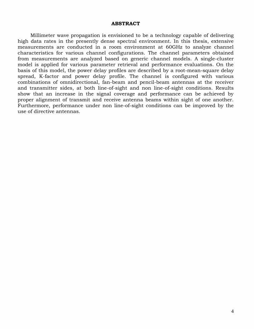
Millimeter wave propagation is envisioned to be a technology capable of delivering high data rates in the presently dense spectral environment. In this thesis, extensive measurements are conducted in a room environment at 60GHz to analyze channel

characteristics for various channel configurations. The channel parameters obtained from measurements are analyzed based on generic channel models. A single-cluster model is applied for various parameter retrieval and performance evaluations. On the

basis of this model, the power delay profiles are described by a root-mean-square delay spread, K-factor and power delay profile. The channel is configured with various

combinations of omnidirectional, fan-beam and pencil-beam antennas at the receiver and transmitter sides, at both line-of-sight and non line-of-sight conditions. Results show that an increase in the signal coverage and performance can be achieved by

proper alignment of transmit and receive antenna beams within sight of one another. Furthermore, performance under non line-of-sight conditions can be improved by the use of directive antennas.

5

DECLARATION

I hereby declare that this is my work and that it has not been submitted before anywhere for the purpose of awarding a degree to the best of my knowledge.

Promise Elechi ........................... ................. Signature date

6

DEDICATION

This work is dedicated to the Almighty God and to the memory of my late mother, Mrs. Helen Chituru Elechi (Nee Orisa)

7

ACKNOWLEDGEMENT I use this opportunity to express my sincere gratitude to Almighty God who gave me the

strength to carry out this work. My profound gratitude goes to Engr. (Dr.) Biebuma J.J. and Mr Eteng A., my thesis supervisors for their personal commitments, sacrifices and words of wisdom which

contributed in no small measure to the realization of this thesis. I equally thank Prof. A.O. Ibe, the postgraduate co-ordinator and Engr. (Dr.) Kamalu Ugochukwu A., the head of the department of Electrical/Electronic Engineering and his

academic and non-academic staff for their encouragements. I wish to thank my fiancée Miss Kate Chioma Amadi and my brothers and sisters

especially Miss Cynthia Obinichi, Mr. Alswell Kemjika Elechi, Miss Adanne Elechi, Miss Faithful Elechi, Miss Rita Ebere Elechi, my cousin Mrs Elizabeth Chidi Nnwoka, my oga Barrister Alwell Ezebunwo and my coursemates, Engrs. Armiyau Braimah, Igbekele

Omotayo and Saliu Mohammed for their kind assistance, encouragements, patience, understanding and love during the programme.

Similar thanks goes to my parents, brothers and sisters and others for their understanding and moral support. I am indebted to the following staff of Daewoo Nigeria Limited, Bayelsa State, for their

numerous contributions towards the realization of my academic dream: Hezekiah Kointeinbo-Ofori, Egeonu Innocent, S.Y. Lee, C.S. Kim, H.M. Kim, B.S. Oh, K.U. Bae,

J.K. Park, Nelson Tuotamuno, Peter Gogo Biekpo, John Ovie Eze and Kingsway Nwuche. Finally, I wish to specially thank Engr. and Mrs Nehemiah Chinenye, Ojadi my bosom

friends for standing by me throughout the academic period.

8

TABLE OF CONTENT Title page i

Certification iii Abstract iv Declaration v

Dedication vi Acknowledgement vii Table of Content viii

List of Figures x List of Tables xiii

CHAPTER 1: INTRODUCTION 1 1.1 Background of Study 1 1.2 Statement of the problem 2

1.3 Objective of Study 2 1.4 Significance of Study 3 1.5 Scope of Study 4

CHAPTER 2: LITERATURE REVIEW 5 2.1 Historical review of wireless communication 5

2.2 Advantages of millimetre wave radio over ultra wideband technology. 6

2.3 Studies in millimetre wave radio technology 8

CHAPTER 3: METHODOLOGY 13 3.1 Description of the Experiment Environment. 13

3.2 Channel Model 20 3.3 Calculation 23 3.3.1 Received power 23

3.3.2 K-factor 24 3.3.3 Estimating the RMS delay spread from frequency-domain level crossing rate

25

3.3.4 Application to channel measurements 26 3.3.5 Power Delay Profile 28

CHAPTER 4: RESULTS AND DISCUSSION 29 4.1 Received Power 29 4.2 K-factor and Root Mean Square Delay Spread 44

4.3 Power Delay Profile 69 4.4 Maximum Excess Delays and Number of Multipath 74

Components CHAPTER 5: CONCLUSION 75 5.1 Conclusion 75

5.2 Recommendation 76 REFERENCES 77 APPENDICES 79

9

LIST OF FIGURES Figure 3.1(a) and (b): HP8510C network analyzer 15

Figure 3.2: Plan view of the rooms 19 Figure 4.1:The received power over the travel distance of the first arrived path of

the omn. antenna (1.4/1.4) 30

Figure 4.2: The received power over the travel distance of the first arrived path of the omn. Antenna (1.9/1.4) 31

Figure 4.3: The received power over the travel distance of the first arrived path of the

omn. antenna(2.4/1.4) 32 Figure 4.4: The received power over the travel distance of the first arrived path of the

omn antenna NLOS (1.4/1.4) 33 Figure 4.5: The received power over the travel distance of the first arrived path of the

omn. antenna NLOS (1.9/1.4). 34

Figure 4.6: The received power over the travel distance of the first arrived path of the omn. antenna NLOS (2.4/1.4) 35

Figure 4.7: The received power over the travel distance of the first arrived path of the

omn antenna for free space 36 Figure 4.8: The received power over the travel distance of the first arrived path for the

Fan-Omn antennas. 38 Figure 4.9: The received power over the travel distance of the first arrived path for the

Fan-Fan antennas. 39

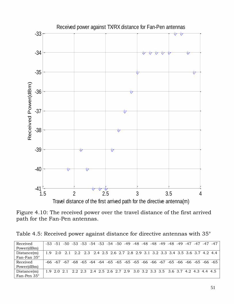
Figure 4.10: The received power over the travel distance of the first arrived path for the Fan-Pen antennas. 40

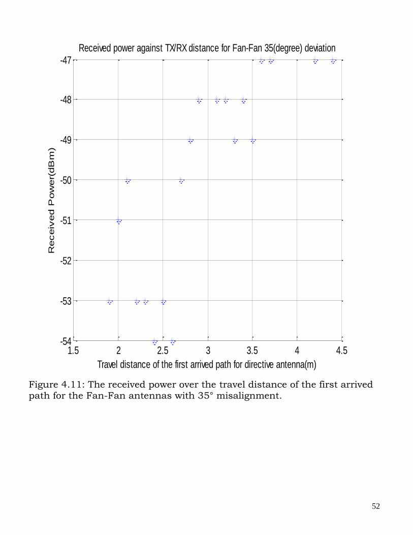
Figure 4.11: The received power over the travel distance of the first arrived path for the Fan-Fan (35°) 41

Figure 4.12: The received power over the travel distance of the first arrived path for the

Fan-Pen (35°) 42 Figure 4.13: The K-factor over the travel distance of the first arrived path of the omn.

antenna (1.4/1.4). 44

Figure 4.14: The K-factor over the travel distance of the first arrived path of the omn. antenna (1.9/1.4) 45

Figure 4.15: The K-factor over the travel distance of the first arrived path of the omn. antenna (2.4/1.4) 46

Figure 4.16: The K-factor over the travel distance of the first arrived path of the omn.

antenna NLOS (1.4/1.4). 48 Figure 4.17: The K-factor over the travel distance of the first arrived path of the omn.

antenna NLOS (1.9/1.4). 49 Figure 4.18: The K-factor over the travel distance of the first arrived path of the omn.

antenna NLOS (2.4/1.4). 50

Figure 4.19: The K-factor over the travel distance of the first arrived path for the Fan-Omn antennas. 51

Figure 4.20: The K-factor over the travel distance of the first arrived path for the Fan-

Fan antenna. 52 Figure 4.21: The K-factor over the travel distance of the first arrived path for the Fan-

Pen antennas. 53 Figure 4.22: The K-factor over the travel distance of the first arrived path for the Fan-

Fan antennas with (35°) 54

Figure 4.23: The K-factor over the travel distance of the first arrived path for the Fan-Pen antennas with (35°) 55

10

Figure 4.24: The RMS delay spread over the travel distance of the first arrived path of the omn. antenna (1.4/1.4). 58

Figure 4.25: The RMS delay spread over the travel distance of the first arrived path of the omn. antenna (1.9/1.4). 59

Figure 4.26: The RMS delay spread over the travel distance of the first arrived path of

the omn. antenna (2.4/1.4). 60 Figure 4.27: RMS delay spread over the travel distance of the first arrived path of the

omn. antenna NLOS(1.4/1.4). 61

Figure 4.28: RMS delay spread over the travel distance of the first arrived path of the omn. antenna NLOS(1.9/1.4). 62

Figure 4.29: RMS delay spread over the travel distance of the first arrived path of the omn. antenna NLOS(2.4/1.4). 63

Figure 4.30: RMS delay spread over the travel distance of the first arrived path for the

Fan-Omn antennas. 64 Figure 4.31: RMS delay spread over the travel distance of the first arrived path for the

Fan-Fan antennas. 65

Figure 4.32: RMS delay spread over the travel distance of the first arrived path for the Fan-Pen antennas. 66

Figure 4.33: The RMS delay spread over the travel distance of the first arrived path for the Fan-Fan antennas (35°) 67

Figure 4.34: The RMS delay spread over the travel distance of the first arrived path for

the Fan-Pen antennas (35°) 68 Figure 4.35: The Average power delay profiles shape for Fan-Pen antennas configuration

69 Figure 4.36: The Average power delay profiles shape for Fan-Pen antennas with 35°

misalignment configuration. 70

Figure 4.37: The Average power delay profiles shape for Omn-Omn configuration 71

11

LIST OF TABLES Table 3.1: Antenna parameters. 16

Table 3.2: Measurement configurations. 18 Table 4.1: Received power data under line of sight condition. 29 Table 4.2: Received power data under non line of sight condition. 33

Table 4.3: Received power data for free space 35 Table 4.4: Received power against distance for directive antennas37

Table 4.5: Received power against distance for directive antennas with 35° misalignment. 40

Table 4.6: K-factor against travel distance under LOS condition 44 Table 4.7: K-factor against travel for NLOS condition 47 Table 4.8: K-factor against travel distance for directive antennas. 51

Table 4.9: K-factor against distance for directive antenna with 35° misalignment 53

Table 4.10: RMS delay spread against distance under LOS condition 57

Table 4.11: RMS delay spread against distance under NLOS condition 60

Table 4.12: RMS delay spread against distance for directive antennas

63 Table 4.13: RMS delay spread against distance for directive antennas (35°)

66 Table 4.14: Normalized average PDP over Time delay 69

Table 4.15: The mean values of K, σ max, Bc, N and the log-distance model parameters {PLo, n, Ώ} for various configurations. 73

12

CHAPTER 1

INTRODUCTION

1.1 Background of Study

With the rapid progress in telecommunications, more and more

services are provided on the basis of broadband communications, such

as video services and high speed internet. The distributed wireless

communication system is a new architecture for a wireless access with

distributed antennas, distributed processors, and distributed controls.

With the worldwide construction of optical fiber-based backbone

networks providing almost unlimited communications capability, the

limited throughput of the subscribers loop becomes one of the most

stringent bottlenecks. Compared to the capacity of the backbone

network, which is measured by tens of gigabit per second, the

throughput of the subscriber loop is much lower, only up to hundreds

of megabits per second for wired systems (including fixed wireless

access).

However, Chong and Yong (2007), suggest that millimeter wave

technology can improve this low throughput of the subscribers loop.

Millimeter waves generally correspond to the electromagnetic spectrum

between 30GHz to 300GHz, with wavelengths between one and ten

millimeters. In the context of wireless communication, millimeter waves

13

generally correspond to a few bands of spectrum near 30GHz, 60GHz

and 94GHz.

1.2 Statement of Problem

According to the Shannon capacity theorem:

(1)

where C is the channel capacity, B is the bandwidth and SNR is the

signal power to noise power ratio. An increase in bandwidth or signal

power to noise power ratio or both can improve the channel capacity

for a specific operating distance. But the basic hindrance to the

improvement of channel capacity by bandwidth adjustment is that

conventionally available spectrum is limited. This imposes a limit to the

achievable channel capacity improvement.

As Chong and Yong (op.cit) have suggested, the solution may lie in

the use of a different spectral window, albeit millimeter wave, to

achieve greater channel capacity. What is however not very clear, is the

suitability of millimeter waves for communication.

1.3 Objective of Study

The objective of this study is to analyze the channel

characteristics for various channel configurations of millimeter wave

transmissions at 60GHz. Specifically, this study will:

14

(1) Experimentally determine channel parameters to describe the power

profiles, with which the 60GHz channel will be analyzed, and

consequently;

(2) Determine the most suitable antenna configuration for this channel.

1.4 Significance of Study

The power delay profile is a function characterizing the spread of

average received power as a function of delay; therefore it is important

to determine the time interval between transmission of a signal

through a communication channel and reception. The power delay

profile shows the maximum delay in a channel and so accounts for

the suitability of a channel. Its determination, in the context, would

provide insight into the capabilities of the 60GHz spectral window.

There are virtually no communications services operating in the

60GHz range. Therefore a successful implementation of the millimeter

wave scheme will be relatively interference free, and will pose no

interference to other existing technologies. The use of this spectral

window will make large amounts of bandwidth available for wireless

communication. Incorporating millimeter wave technology into

distributed wireless systems will remove the low throughput bottleneck

associated with the subscriber loops.

15

1.5 Scope of Study

Although this study is geared towards obtaining a workable

channel configuration at 60GHz, this thesis does not consider the

effects of atmospheric oxygen, humidity, fog and rain within this

spectral window. Recent studies, however, show that the 60GHz

channel has negligible signal loss due to atmospheric oxygen – about

0.2dB/km (Lim et. al, 2007).

16

CHAPTER 2

LITERATURE REVIEW

2.1 Historical Review of Wireless Communication

Wireless communications is not new; it has been around for

decades. Heinrich Hertz, Nikola Tesla, Gugliemo Marconi, and others

experimented with the transmission and reception of radio waves in the

19th century. The actual birth of radio occurred in 1890 when J.C.

Bose was experimenting with millimeter wave signals at just the time

when his contemporaries like Marconi were inventing radio

communications. In 1897, Marconi first demonstrated that radio

communication could provide wireless communication between ships

(Sadiku, 2002).

The development of wireless communications can be regarded as

taking place in three phases. The period spanning 1907 to 1945 can be

regarded as the pioneer phase. In 1907, Lee De Forest invented the

triode, which made possible the first amplitude modulation (AM)

scheme and the amplification of weak radio signals. Edwin Armstrong,

invented frequency modulation (FM) in 1935. World War II was a

stimulus to wireless communications, leading to the subsequent

development of consumer radio and television systems.

17

The period spanning 1946 to 1968 can be considered as the initial

commercial phase, although the first regular commercial radio

broadcast began in 1920. The third phase began 1969. This phase

includes the beginning of cellular, mobile, satellite and personal

communication systems. The recent generation of cellular services use

Time Division Multiple Access (TDMA), Code Division Multiple Access

(CDMA), narrow-band Frequency Division Multiple Access (FDMA), and

Collision Sense Multiple Access (CSMA) spread spectrum (Pozar, 2001),

which are all mostly based on the principle of microwave propagation.

2.2 Advantages of Millimeter Wave Radio over Ultra Wideband Technology.

It is a fact that the ultra-wideband (UWB) is also being used as a

means of improving channel capacity. But the 60GHz millimeter wave

band has the following advantages over it.

(1) The low emission and impulsive nature of UWB radio leads to

enhanced security in communication. UWB is able to deliver high-

speed multimedia wirelessly making it suitable for WPANs. However,

one of the most challenging issues for UWB is that international

coordination regarding the operating spectrum is difficult to achieve

and the IEEE standards are not accepted worldwide. This spectral

difficulty will deeply shape the landscape of WPANs in the future.

18

Spectrum allocation is not an issue for 60GHz WPANs. This is one of

the reasons for 60GHz millimeter wave.

(2) Inter-system interference is another concern. The UWB band is

overlaid over the 2.4- and 5-GHz bands used for increasingly

deployed WLANs, thus the mutual interferences would be getting

worse and worse. According to Nan Guo, et al (2007), inter-system

interference problem exists in Europe and Japan. In order to protect

existing wireless systems operating in different regions, regulatory

bodies in these regions are working on their requirements for UWB

implementation. For the 60GHz band, worldwide harmonization is

possible but it is impossible for a regional UWB radio to work in

another region.

(3) Data-rate limitation is also a concern. Currently, the multiband

OFDM (MB-OFDM) UWB system can provide maximum data rate of

480MB/s which can only support compressed video. 60GHz can

easily go over 2GB/s such as in high definition multimedia interface

(HDMI).

(4) Variation of received signal strength over a given spectrum can be a

bothering factor. For the MB-OFDM UWB system, there are 5 band

groups covering a frequency range from 3.1GHz to 10.6GHz.

According to the Friis propagation rule, given the same transmitted

19

power, propagation attenuation is inversely proportional to the

square of a group center frequency. If band group 1 can cover 10m,

coverage range for band group 5 is only 1.56m. On the other hand,

because of relatively smaller change in frequency, coverage range

does not change dynamically for the 60GHz radio.

2.3 Studies in Millimeter Wave Radio Technology

Yong and Chong, (2007) provide a generic overview of the current

status of the millimetre wave radio technology, in order to support the

multigigabit wireless applications. They envisioned that the 60GHz

radio will be one of the important candidates for the next generation

wireless systems as well as the role of antennas in establishing a

reliable communication link. Despite the many advantages offered and

high potentials application envisaged, the authors did not report on the

number of technical challenges and open issues that must be solved

prior to the successful deployment of this technology.

Nan Guo et al, (2007) extends the overview by summarizing some

recent works in the area of 60GHz radio system design. Some new

simulation results were reported which showed the impact of the phase

noise on bit-error rate (BER). The authors concluded that phase noise

is a very important factor when considering multigigabit wireless

transmission but did not offer any solution to averting the problem.

20

Lim C.P. et al, (2007) proposed a 60GHz indoor propagation

channel model based on the ray-tracing method. The model is validated

with measurements conducted in indoor environment. The authors

highlighted important parameters such as root mean square (RMS)

delay spread and fading statistics in order to characterize the

behaviour of the millimeter wave multipath propagation channel

extracted from the environment database. The report was mostly based

on a ray-tracing method using spacing between 2GHz and 3GHz

continuous wave in the simulation.

Yang et al, (2007) used a different modeling approach in

characterizing the 60GHz propagation channel. A statistical-based

channel model was proposed based on the extensive measurements

campaign conducted in indoor office environment. Based on that, a

single-cluster power delay profile (PDP) was formed to best characterize

the channel statistics in which the PDP can be parameterized by K-

factor, RMS delay spread and shape parameter under both line-of-sight

(LOS) and non line-of-sight (NLOS) conditions. Various types of

antenna pattern were used but they could not solve the problem of

limited link budget due to high path loss during propagation in

distributed wireless communication.

21

Kvicera and Grabner (2007), investigate the effect of rain

attenuation at 58GHz, based on the large measurement results

collected over a 5-year period. The measurement results obtained were

analysed and compared to the ITU-R recommendations which are valid

for estimating long-term statistics of rain attenuation for frequency up

to 40GHz. The reports are only important for point-to-point fixed

system up to 60GHz based on ITU-R recommendations.

Based on the report by Kvicera and Grabner (2007), Van der

Zanden et al, (2008), addresses the modelling and prediction of rain-

induced bistatic scattering at 60GHz. The factor is important as it

could cause link interference between 60GHz links when rain falls.

They showed that despite the high oxygen attenuation, coupling

between adjacent links caused by bistatic scattering could be

significant even in light rain as it affects distributed wireless

communication.

Mohammadi, et al (2007), proposed a direct conversion

modulator-demodulator for fixed wireless application. Though the

circuit is not for distributed wireless application but explains the basis

for wireless communication. The circuits consist of even harmonic

mixers (EHMs) realized with antiparallel diode pairs (APDPs), where

self-biased APDP is used in order to flatten the conversion loss of the

22

system versus local oscillator (LO) power. The impacts of the baseband

modulating signals (I/Q) imbalances and DC offsets on BER

performance of the system was also considered. A communication link

was built with the proposed modulator-demodulator and experimental

results showed that such a system can be a low-cost and high-

performance Quadrature Amplitude Modulation (16-QAM) transceiver

especially for the local multipoint distribution system (LMDS)

applications.

Tatu and Moldovan, (2007), proposed a practical circuit for the

60GHz radio. In the report, a V-band (the circuit is composed of four

90° hybrid couplers connected by 50Ώ microstrip transmission line)

receiver using an MHMIC multiport circuit was proposed. It was

demonstrated that the combination of multiport circuits with power

detectors and two different amplifiers can replace the conventional

mixer in a low-cost heterodyne or homodyne architecture. The

operating principle of the proposed heterodyne receiver and

demodulation results of high-speed multiport phase shift keying and

quadrature amplitude modulation (MPSK/QAM) signals were also

discussed. Simulation results showed that an improved overall gain

can be obtained. The authors concluded that such a multiport

heterodyne architecture can enable the compact and low-cost

23

millimetre-wave receivers for the future wireless communications

system.

24

CHAPTER 3

METHODOLOGY

The method of study adopted in this work is to conduct

experiment to understand the behaviour of the channel of a distributed

wireless communication systems. The specific parameters to derive in

this experiment are: Root-mean-square delay spread, K-factor and

power delay profile shape, calculated from the measured received

power in describing the power delay profile. In the course of deriving

this parameters, the combination of omnidirectional antennas, fan-

beam antennas and pencil-beam antennas at the transmitter and

receiver are used in determining the most suitable antenna

configuration in both line-of-sight and non line-of-sight conditions. The

data obtained are interpreted as scatter diagrams showing the

maximum value of points in the analysis of each parameter. Subsection

3.2 shows the analytical relationship between the parameters as can be

obtained based on the experiment conducted in subsection 3.1.

3.1 Description of the Experiment Environment

Aim: The aim of this statistical measurement is to determine the

received power over certain distances, the K-factor which accounts for

fading, the root-mean-square delay spread and the power delay profile

25

which are used to analyze the channel characteristics for various

channel configurations.

Equipments Required: Two network analyzers (HP 8510C), two

Omnidirectional antennas, a Pencil-beam antenna and two Fan-beam

antennas, measurement tapes, Frequency generator and Angle

measurement indicator.

Procedure: The vector network analyzer (HP 8510C) was employed to

measure complex channel frequency responses as seen in figures 3.1

(a) and (b) used in rooms A and B respectively.

3.1(a)

26

3.1(b)

Figures 3.1(a) and (b): HP8510C network analyzer

During measurements, the following steps were adopted to measure

the received power: Select the power in the measurement knob, adjust

the receiving antenna position, send a signal through the transmitting

antenna, and record the received power as well as the distance between

the transmitter and the receiver. Repeat for 20 measurements, after

which the transmitter height is adjusted by 0.5m and the steps are

repeated for three times, the step sweep mode was used and the sweep

time of each measurement was about 20 seconds. Channel impulse

responses were obtained by Fourier transforming the frequency

responses generated by the continuous wave frequency generator into

time domain after a Kaiser window was applied with a sidelobe level of

−44dB.

Note that in all the measurements, the transmit power is 0 dBm.

27

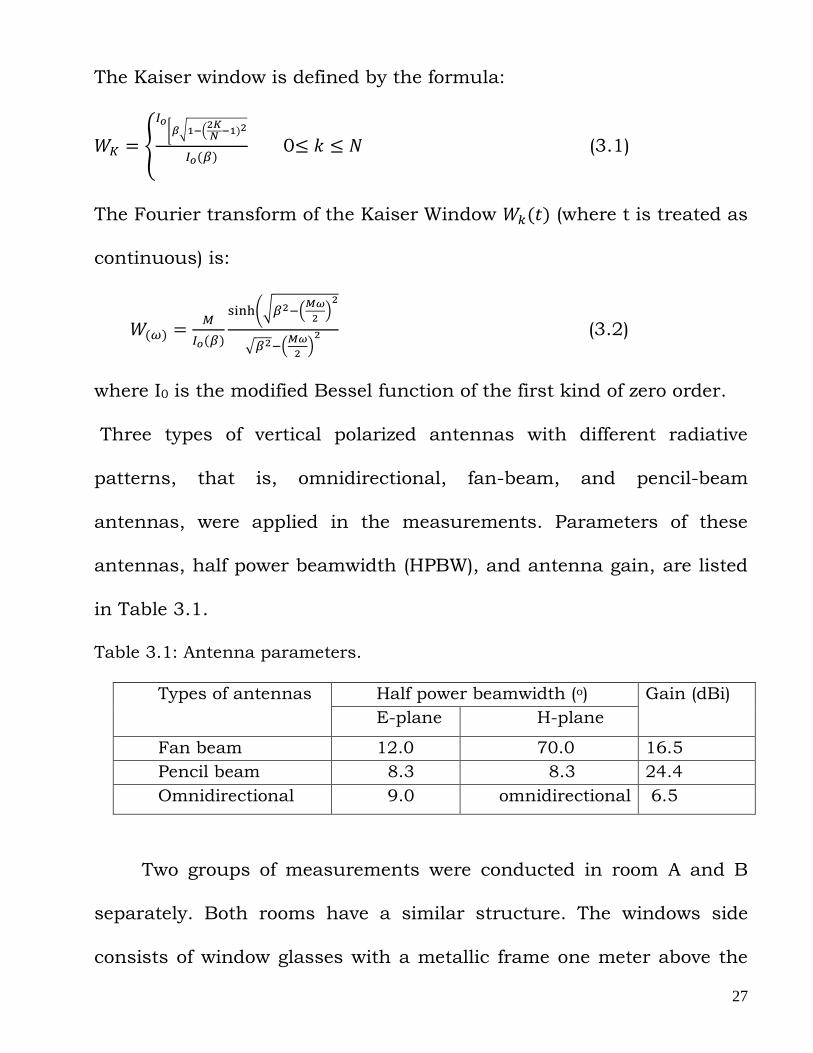
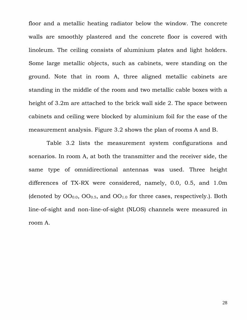
The Kaiser window is defined by the formula:

0 (3.1)

The Fourier transform of the Kaiser Window (where t is treated as

continuous) is:

(3.2)

where I0 is the modified Bessel function of the first kind of zero order.

Three types of vertical polarized antennas with different radiative

patterns, that is, omnidirectional, fan-beam, and pencil-beam

antennas, were applied in the measurements. Parameters of these

antennas, half power beamwidth (HPBW), and antenna gain, are listed

in Table 3.1.

Table 3.1: Antenna parameters.

Types of antennas Half power beamwidth (o) Gain (dBi)

E-plane H-plane

Fan beam 12.0 70.0 16.5

Pencil beam 8.3 8.3 24.4

Omnidirectional 9.0 omnidirectional 6.5

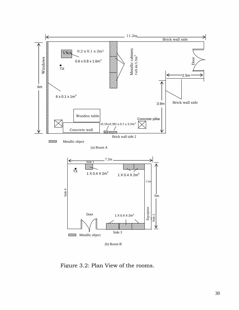
Two groups of measurements were conducted in room A and B

separately. Both rooms have a similar structure. The windows side

consists of window glasses with a metallic frame one meter above the

28

floor and a metallic heating radiator below the window. The concrete

walls are smoothly plastered and the concrete floor is covered with

linoleum. The ceiling consists of aluminium plates and light holders.

Some large metallic objects, such as cabinets, were standing on the

ground. Note that in room A, three aligned metallic cabinets are

standing in the middle of the room and two metallic cable boxes with a

height of 3.2m are attached to the brick wall side 2. The space between

cabinets and ceiling were blocked by aluminium foil for the ease of the

measurement analysis. Figure 3.2 shows the plan of rooms A and B.

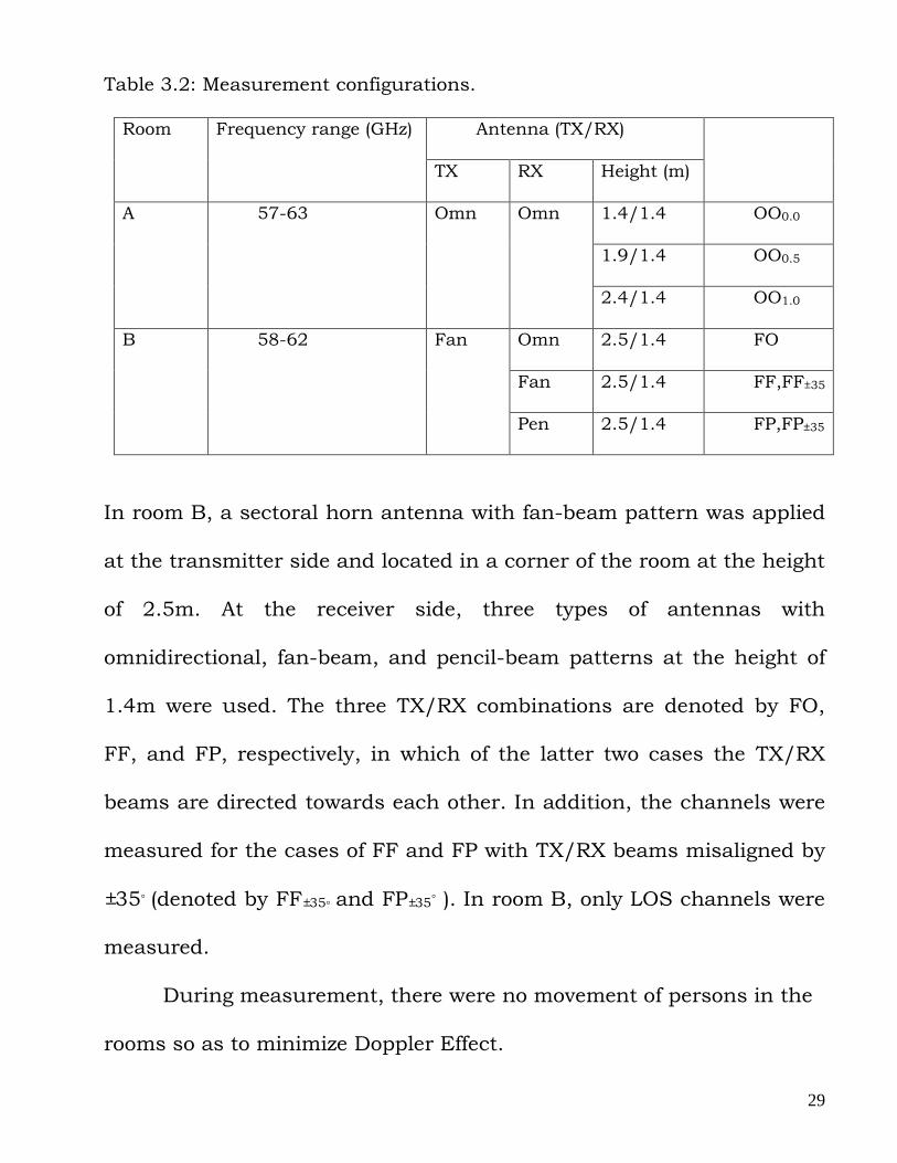
Table 3.2 lists the measurement system configurations and

scenarios. In room A, at both the transmitter and the receiver side, the

same type of omnidirectional antennas was used. Three height

differences of TX-RX were considered, namely, 0.0, 0.5, and 1.0m

(denoted by OO0.0, OO0.5, and OO1.0 for three cases, respectively.). Both

line-of-sight and non-line-of-sight (NLOS) channels were measured in

room A.

29

Table 3.2: Measurement configurations.

Room Frequency range (GHz) Antenna (TX/RX)

TX RX Height (m)

A 57-63 Omn Omn 1.4/1.4 OO0.0

1.9/1.4 OO0.5

2.4/1.4 OO1.0

B 58-62 Fan Omn

2.5/1.4 FO

Fan

2.5/1.4 FF,FF±35

Pen 2.5/1.4 FP,FP±35

In room B, a sectoral horn antenna with fan-beam pattern was applied

at the transmitter side and located in a corner of the room at the height

of 2.5m. At the receiver side, three types of antennas with

omnidirectional, fan-beam, and pencil-beam patterns at the height of

1.4m were used. The three TX/RX combinations are denoted by FO,

FF, and FP, respectively, in which of the latter two cases the TX/RX

beams are directed towards each other. In addition, the channels were

measured for the cases of FF and FP with TX/RX beams misaligned by

±35◦ (denoted by FF±35◦ and FP±35

◦ ). In room B, only LOS channels were

measured.

During measurement, there were no movement of persons in the

rooms so as to minimize Doppler Effect.

30

11.2m Brick wall side 1

VNA 0.2 x 0.1 x 2m3

0.6 x 0.8 x 1.6m3

TX

6 x 0.1 x 1m3

Wooden table

Concrete wall

(0.15+0.35) x 0.1 x 3.2m3

3.2

Concrete pillar

3.9m Brick wall side 3,4 4

2.5m

Do

or

Met

alli

c ca

bin

ets

1x

0.4

x3

.2m

3

Win

dow

s

sid

e

6m

Metallic object

Brick wall side 2

1 X 0.4 X 2m3

1 X 0.4 X 2m3

7.2m Side 1

Sid

e 4

Equ

ipm

e

nt

Sid

e 2

1.5m

6m

1 X 0.4 X 2m3 Door

Metallic object Side 3

(b) Room B

Figure 3.2: Plan View of the rooms.

TX

(a) Room A

31

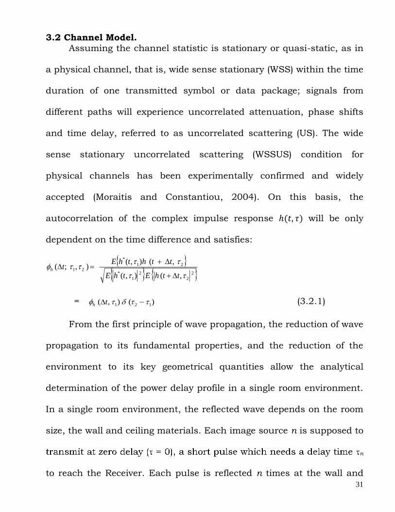
3.2 Channel Model. Assuming the channel statistic is stationary or quasi-static, as in

a physical channel, that is, wide sense stationary (WSS) within the time

duration of one transmitted symbol or data package; signals from

different paths will experience uncorrelated attenuation, phase shifts

and time delay, referred to as uncorrelated scattering (US). The wide

sense stationary uncorrelated scattering (WSSUS) condition for

physical channels has been experimentally confirmed and widely

accepted (Moraitis and Constantiou, 2004). On this basis, the

autocorrelation of the complex impulse response will be only

dependent on the time difference and satisfies:

2

2

2

1

*

21

*

21

,(),(

,(),(),;(

tthEthE

tththEth

= )(),( 121 th

(3.2.1)

From the first principle of wave propagation, the reduction of wave

propagation to its fundamental properties, and the reduction of the

environment to its key geometrical quantities allow the analytical

determination of the power delay profile in a single room environment.

In a single room environment, the reflected wave depends on the room

size, the wall and ceiling materials. Each image source n is supposed to

n

to reach the Receiver. Each pulse is reflected n times at the wall and

32

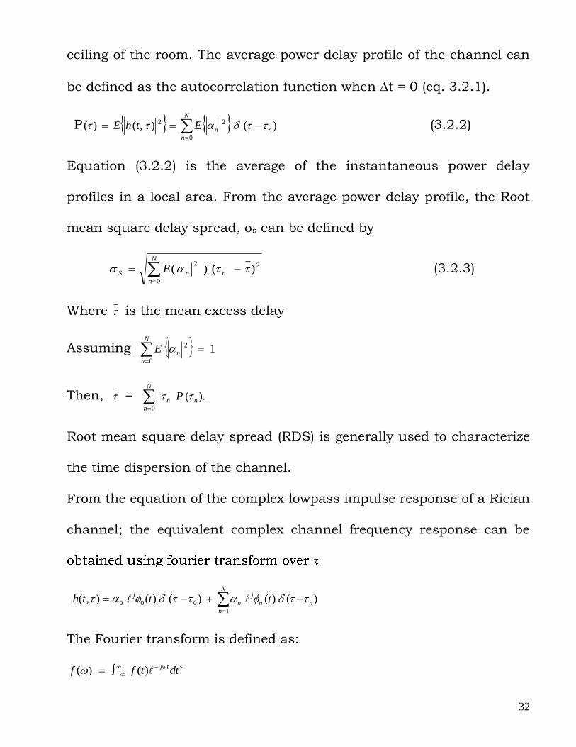
ceiling of the room. The average power delay profile of the channel can

be defined as the autocorrelation function when t = 0 (eq. 3.2.1).

P )(),()( 2

0

2

nn

N

n

EthE

(3.2.2)

Equation (3.2.2) is the average of the instantaneous power delay

profiles in a local area. From the average power delay profile, the Root

mean square delay spread, σs can be defined by

22

0

)()(

nn

N

n

S E (3.2.3)

Where is the mean excess delay

Assuming 12

0

n

N

n

E

Then, = ).(0

nn

N

n

P

Root mean square delay spread (RDS) is generally used to characterize

the time dispersion of the channel.

From the equation of the complex lowpass impulse response of a Rician

channel; the equivalent complex channel frequency response can be

),( th

N

n

nn

j

n

j tt1

000 )()()()(

The Fourier transform is defined as:

`)()( dttff jwt

33

N

n

jw

n

tj

n

jw

o

tj

o ddf no

1

)()()()()(

N

n

jw

n

tj

n

jw

o

tj

o dd no

1

)()())(()(

N

n

n

jwtj

no

jtj

o dd no

1

)()()()(

Using the sampling property of the impulse function:

)()()( oo

b

a tfdttttf

N

n

jwtj

n

jwtj

onnoo

1

)()(

N

n

wtj

n

wtj

onnoo

1

))(())((

N

n

wtj

nnn

0

))((

But, f 2

N

n

ftj

nnn

0

)2)((

H

N

n

nn

j

n ftft0

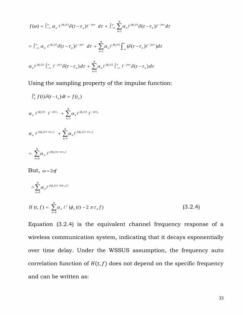
)2)((),( (3.2.4)

Equation (3.2.4) is the equivalent channel frequency response of a

wireless communication system, indicating that it decays exponentially

over time delay. Under the WSSUS assumption, the frequency auto

correlation function of does not depend on the specific frequency

and can be written as:

34

2

2

2

1

*

21

*

21

),(),(

),(),(),(

fttHEftHE

fttHftHEfft jH

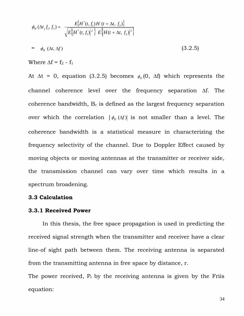
= ),( ftH (3.2.5)

Where f = f2 - f1

At t = 0, equation (3.2.5) becomes H (0, f) which represents the

channel coherence level over the frequency separation f. The

coherence bandwidth, Bc is defined as the largest frequency separation

over which the correlation | )( fH is not smaller than a level. The

coherence bandwidth is a statistical measure in characterizing the

frequency selectivity of the channel. Due to Doppler Effect caused by

moving objects or moving antennas at the transmitter or receiver side,

the transmission channel can vary over time which results in a

spectrum broadening.

3.3 Calculation

3.3.1 Received Power

In this thesis, the free space propagation is used in predicting the

received signal strength when the transmitter and receiver have a clear

line-of sight path between them. The receiving antenna is separated

from the transmitting antenna in free space by distance, r.

The power received, Pr by the receiving antenna is given by the Friis

equation:

35

(3.3.1)

Where Pt is the transmitted power, Gr is the receiving antenna gain, Gt

is the transmitting antenna gain and λ is the wavelength of the

transmitted signal.

λ =

(3.3.2)

where C = 3 108 and

Equation 3.3.1 is commonly expressed in logarithmic form and if all

the terms are expressed in decibels (dB). Equation 3.3.1 can be written

in the logarithmic form as:

(3.3.3)

Where P is the power in dB, G is gain in dB and Lo is the free space loss in

dB.

The free space path loss is obtained directly from equation 3.3.1 as

(3.3.4)

3.3.2 K-Factor The K-factor is the ratio of the powers contributed by the steady

path to the scattered path. The power contributed by the dominant

path is derived by adding the powers within the resolution bin of the

dominant path and is known as the steady path power. The mean of

the transmitted powers outside the resolution bin is known as the

36

scattered path power. The K-factor is calculated for each measurement

in 3.1 using the formula below.

To ensure that there is less fading in the channel, the K-factor must be

greater than 8 (K ).

3.3.3 Estimating the Root-Mean-Square Delay Spread from Frequency-Domain Level Crossing Rate The root-mean-square (RMS) delay spread is probably the most

important single measure for the delay time extent of a multipath radio

channel (Witrisal, et al, 1998). Since the impulse response (IR) and the

transfer function (TF) of a channel are related by the Fourier transform,

it is intuitively understandable that the transfer function's magnitude

shows more fades per bandwidth. There exists a well-defined

relationship between the so-called level crossing rate in the frequency-

domain and the RMS delay spread (Rrms), written as:

(3.3.5)

As seen from this equation, Rrms and the LCRf are proportional, where

the proportionality factor is a function of:

(1) the Rician K-factor, K

37

(2) the threshold value at which the LCRf is determined, r' (r' is

normalized to the RMS amplitude value of the transfer function)

(3) and the channel model, expressed by u. (This influence is very small,

therefore it can be neglected.)

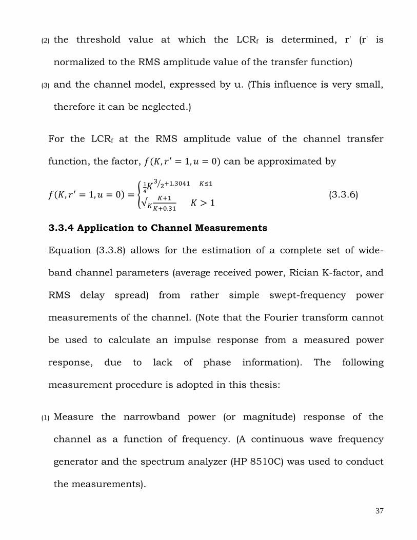
For the LCRf at the RMS amplitude value of the channel transfer

function, the factor, can be approximated by

(3.3.6)

3.3.4 Application to Channel Measurements

Equation (3.3.8) allows for the estimation of a complete set of wide-

band channel parameters (average received power, Rician K-factor, and

RMS delay spread) from rather simple swept-frequency power

measurements of the channel. (Note that the Fourier transform cannot

be used to calculate an impulse response from a measured power

response, due to lack of phase information). The following

measurement procedure is adopted in this thesis:

(1) Measure the narrowband power (or magnitude) response of the

channel as a function of frequency. (A continuous wave frequency

generator and the spectrum analyzer (HP 8510C) was used to conduct

the measurements).

38

(2) Calculate the average received power and the Rician K-factor from the

measured power response.

(3) Count the number of level crossings at a specific threshold, preferably

at the RMS amplitude.

(4) Use equation (3.3.8) for estimating .

An observation bandwidth of 10/Rrms (equivalent to the observation of

approximately 20 level crossings) was allowed for estimating Rrms at

accuracy in the order of 10%. Higher bandwidths can enhance the

accuracy. Alternatively, multiple measurements from within a small

local area such as this measurement rooms can be combined to

increase the observation bandwidth without modifying the

measurement equipment.

Other issues that were considered when applying this method for

channel investigations are:

(1) Influence of the sampling interval of the channel's frequency response:

The sampling interval was selected according to the sampling

theorem; otherwise some fades may be missed when counting the

level crossings.

(2) Influence of measurement equipment noise: Noise may introduce

additional level crossings, which would lead to over estimation of Rrms.

39

The sampling interval mentioned above should be as large as possible

to minimize this noise effect.

3.3.5 Power Delay Profile The received power over time delay for each measurement in 3.1

accounts for the power delay profile of the channel. For each

transmitted signal, the received power is recorded and divided by the

time delay of the signal to reach the receiver.

(3.3.7)

where PDP is the power delay profile, Pri is the ith received power and

i is the ith time delay.

40

CHAPTER 4

RESULTS AND DISSCUSION

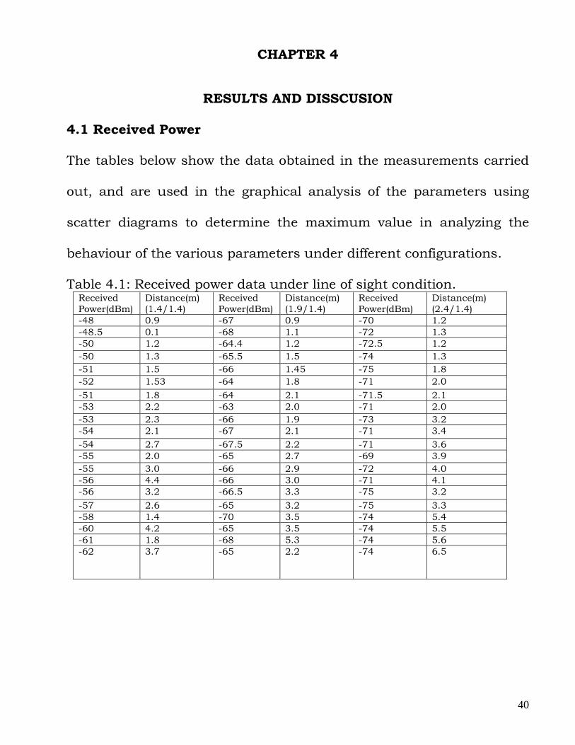
4.1 Received Power

The tables below show the data obtained in the measurements carried

out, and are used in the graphical analysis of the parameters using

scatter diagrams to determine the maximum value in analyzing the

behaviour of the various parameters under different configurations.

Table 4.1: Received power data under line of sight condition. Received

Power(dBm)

Distance(m)

(1.4/1.4)

Received

Power(dBm)

Distance(m)

(1.9/1.4)

Received

Power(dBm)

Distance(m)

(2.4/1.4)

-48 0.9 -67 0.9 -70 1.2

-48.5 0.1 -68 1.1 -72 1.3

-50 1.2 -64.4 1.2 -72.5 1.2

-50 1.3 -65.5 1.5 -74 1.3

-51 1.5 -66 1.45 -75 1.8

-52 1.53 -64 1.8 -71 2.0

-51 1.8 -64 2.1 -71.5 2.1

-53 2.2 -63 2.0 -71 2.0

-53 2.3 -66 1.9 -73 3.2

-54 2.1 -67 2.1 -71 3.4

-54 2.7 -67.5 2.2 -71 3.6

-55 2.0 -65 2.7 -69 3.9

-55 3.0 -66 2.9 -72 4.0

-56 4.4 -66 3.0 -71 4.1

-56 3.2 -66.5 3.3 -75 3.2

-57 2.6 -65 3.2 -75 3.3

-58 1.4 -70 3.5 -74 5.4

-60 4.2 -65 3.5 -74 5.5

-61 1.8 -68 5.3 -74 5.6

-62 3.7

-65

2.2 -74 6.5

41

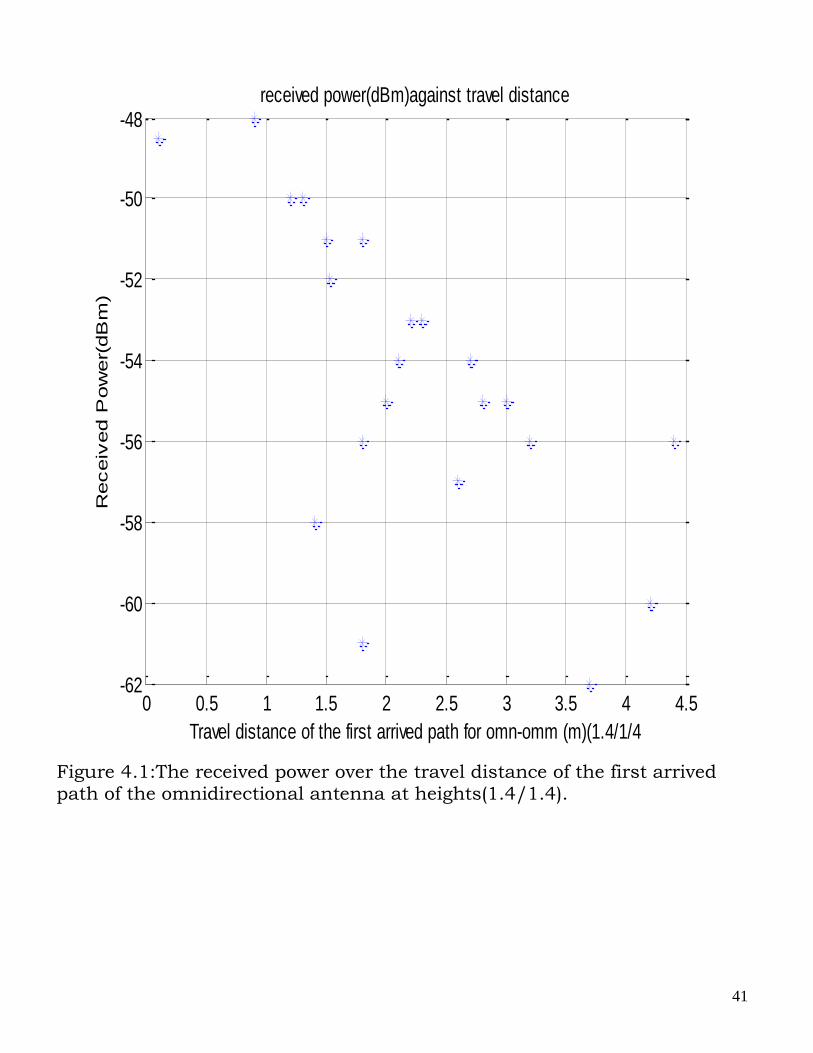
Figure 4.1:The received power over the travel distance of the first arrived path of the omnidirectional antenna at heights(1.4/1.4).

0 0.5 1 1.5 2 2.5 3 3.5 4 4.5-62

-60

-58

-56

-54

-52

-50

-48

Travel distance of the first arrived path for omn-omm (m)(1.4/1/4

Receiv

ed P

ow

er(

dB

m)

received power(dBm)against travel distance

42

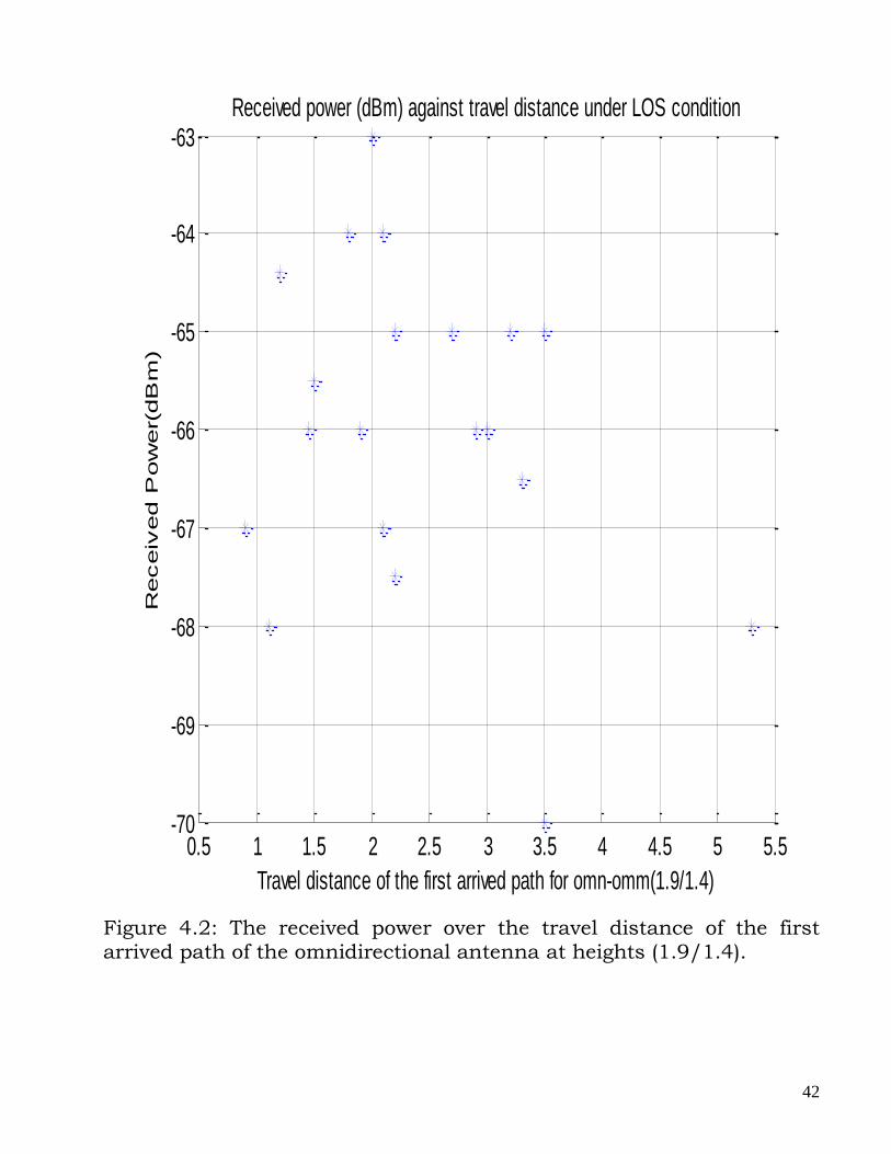
Figure 4.2: The received power over the travel distance of the first arrived path of the omnidirectional antenna at heights (1.9/1.4).

0.5 1 1.5 2 2.5 3 3.5 4 4.5 5 5.5-70

-69

-68

-67

-66

-65

-64

-63

Travel distance of the first arrived path for omn-omm(1.9/1.4)

Receiv

ed P

ow

er(

dB

m)

Received power (dBm) against travel distance under LOS condition

43

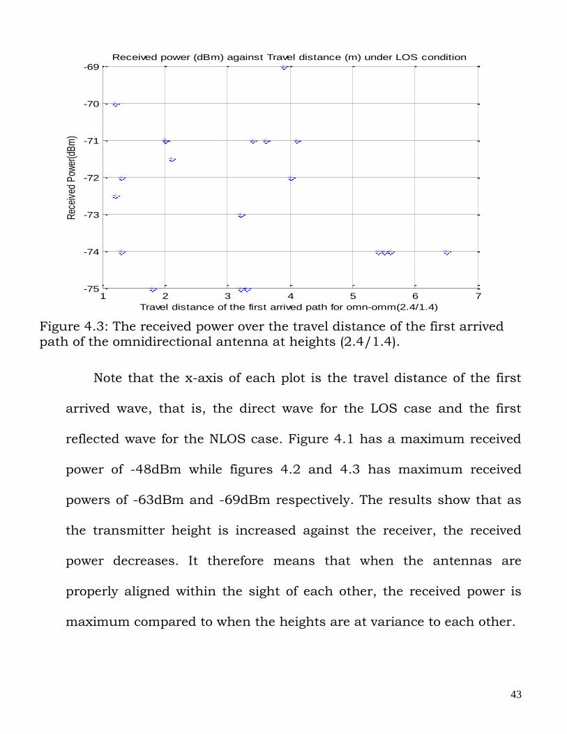
Figure 4.3: The received power over the travel distance of the first arrived path of the omnidirectional antenna at heights (2.4/1.4).

Note that the x-axis of each plot is the travel distance of the first

arrived wave, that is, the direct wave for the LOS case and the first

reflected wave for the NLOS case. Figure 4.1 has a maximum received

power of -48dBm while figures 4.2 and 4.3 has maximum received

powers of -63dBm and -69dBm respectively. The results show that as

the transmitter height is increased against the receiver, the received

power decreases. It therefore means that when the antennas are

properly aligned within the sight of each other, the received power is

maximum compared to when the heights are at variance to each other.

1 2 3 4 5 6 7-75

-74

-73

-72

-71

-70

-69

Travel distance of the first arrived path for omn-omm(2.4/1.4)

Rec

eive

d P

ower

(dB

m)

Received power (dBm) against Travel distance (m) under LOS condition

44

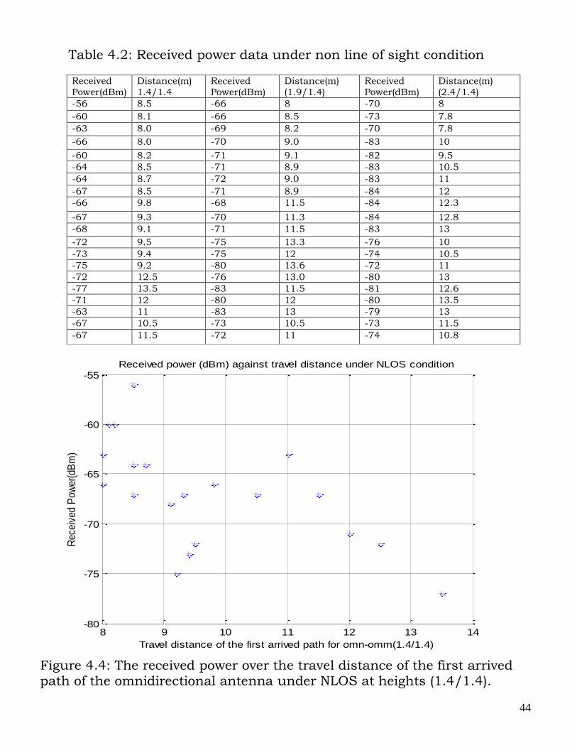
Table 4.2: Received power data under non line of sight condition

Figure 4.4: The received power over the travel distance of the first arrived path of the omnidirectional antenna under NLOS at heights (1.4/1.4).

8 9 10 11 12 13 14-80

-75

-70

-65

-60

-55

Travel distance of the first arrived path for omn-omm(1.4/1.4)

Rec

eive

d P

ower

(dB

m)

Received power (dBm) against travel distance under NLOS condition

Received

Power(dBm)

Distance(m)

1.4/1.4

Received

Power(dBm)

Distance(m)

(1.9/1.4)

Received

Power(dBm)

Distance(m)

(2.4/1.4)

-56 8.5 -66 8 -70 8

-60 8.1 -66 8.5 -73 7.8

-63 8.0 -69 8.2 -70 7.8

-66 8.0 -70 9.0 -83 10

-60 8.2 -71 9.1 -82 9.5

-64 8.5 -71 8.9 -83 10.5

-64 8.7 -72 9.0 -83 11

-67 8.5 -71 8.9 -84 12

-66 9.8 -68 11.5 -84 12.3

-67 9.3 -70 11.3 -84 12.8

-68 9.1 -71 11.5 -83 13

-72 9.5 -75 13.3 -76 10

-73 9.4 -75 12 -74 10.5

-75 9.2 -80 13.6 -72 11

-72 12.5 -76 13.0 -80 13

-77 13.5 -83 11.5 -81 12.6

-71 12 -80 12 -80 13.5

-63 11 -83 13 -79 13

-67 10.5 -73 10.5 -73 11.5

-67 11.5 -72 11 -74 10.8

45

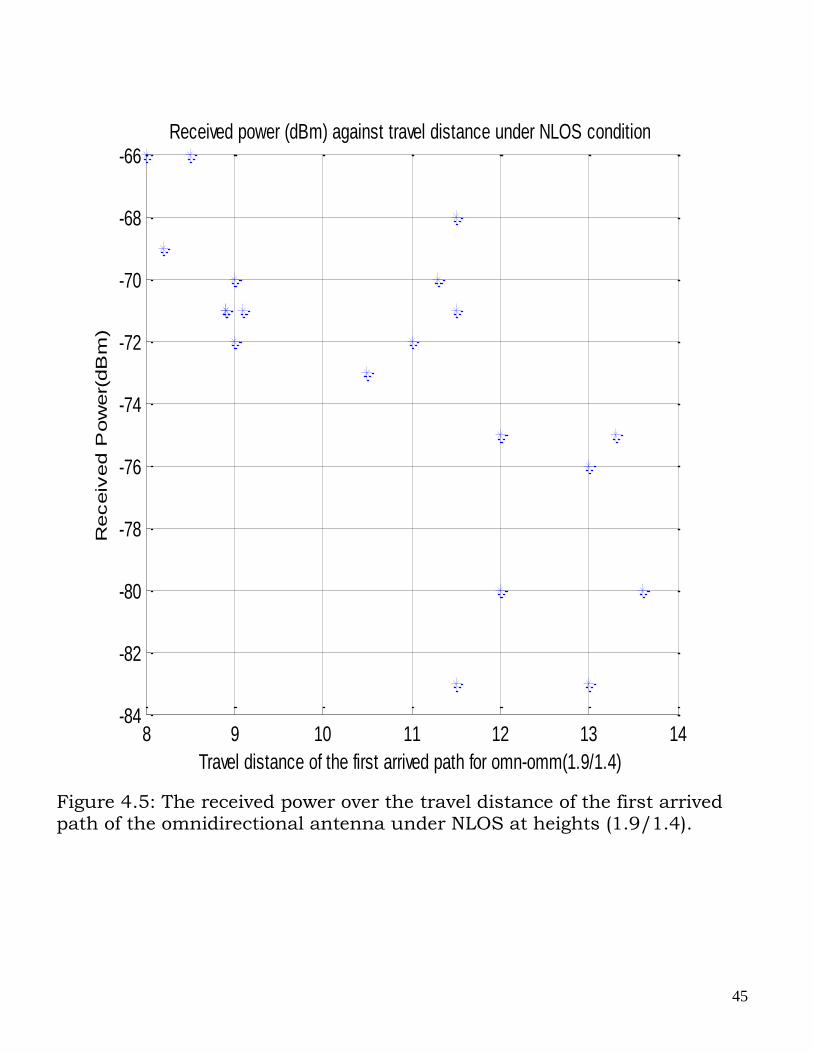
Figure 4.5: The received power over the travel distance of the first arrived path of the omnidirectional antenna under NLOS at heights (1.9/1.4).

8 9 10 11 12 13 14-84

-82

-80

-78

-76

-74

-72

-70

-68

-66

Travel distance of the first arrived path for omn-omm(1.9/1.4)

Receiv

ed P

ow

er(

dB

m)

Received power (dBm) against travel distance under NLOS condition

46

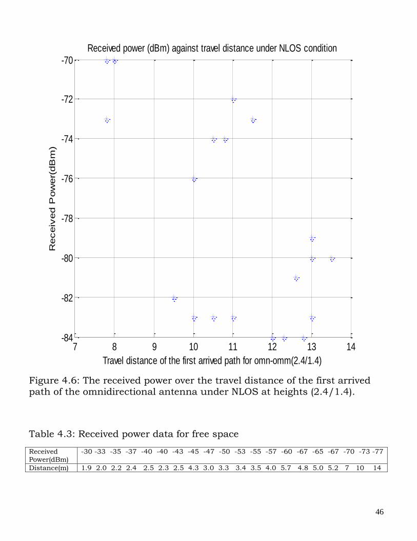
Figure 4.6: The received power over the travel distance of the first arrived path of the omnidirectional antenna under NLOS at heights (2.4/1.4).

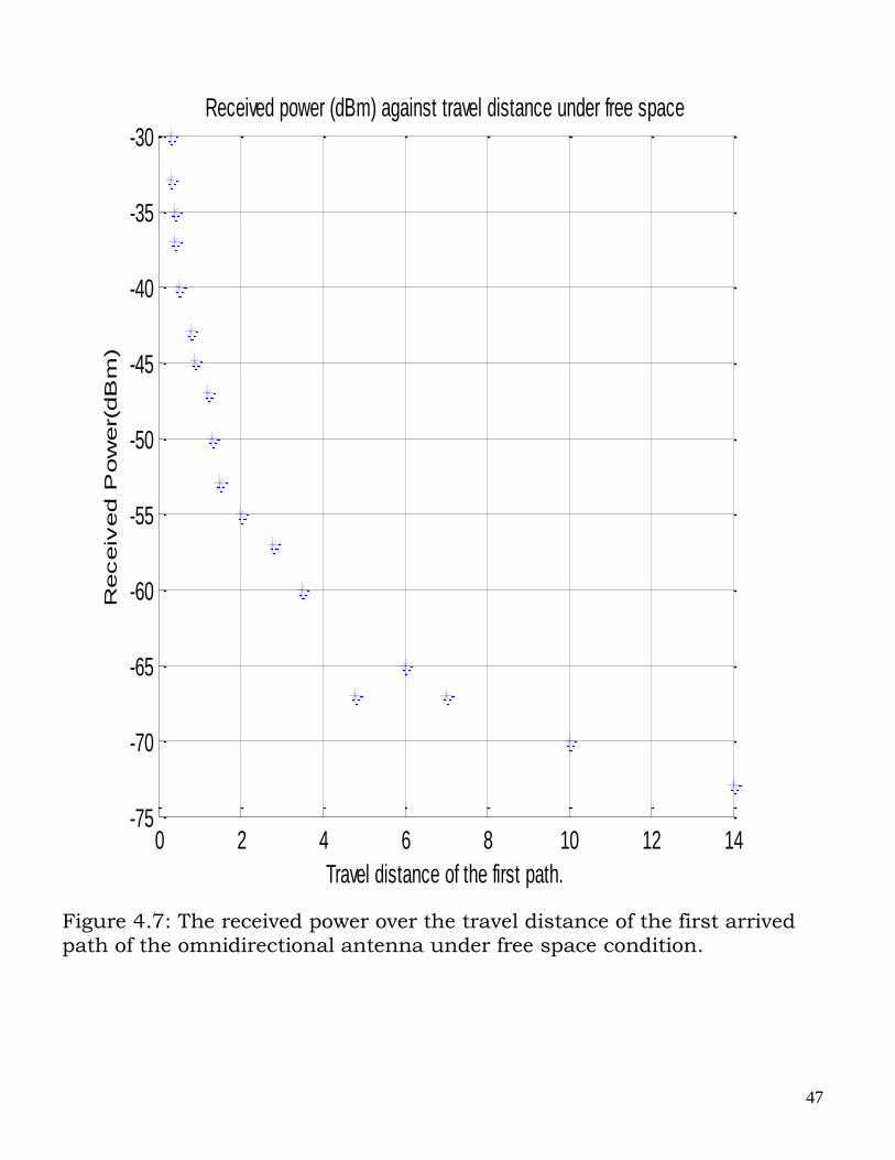
Table 4.3: Received power data for free space

Received

Power(dBm)

-30 -33 -35 -37 -40 -40 -43 -45 -47 -50 -53 -55 -57 -60 -67 -65 -67 -70 -73 -77

Distance(m) 1.9 2.0 2.2 2.4 2.5 2.3 2.5 4.3 3.0 3.3 3.4 3.5 4.0 5.7 4.8 5.0 5.2 7 10 14

7 8 9 10 11 12 13 14-84

-82

-80

-78

-76

-74

-72

-70

Travel distance of the first arrived path for omn-omm(2.4/1.4)

Receiv

ed P

ow

er(

dB

m)

Received power (dBm) against travel distance under NLOS condition

47

Figure 4.7: The received power over the travel distance of the first arrived path of the omnidirectional antenna under free space condition.

0 2 4 6 8 10 12 14-75

-70

-65

-60

-55

-50

-45

-40

-35

-30

Travel distance of the first path.

Receiv

ed P

ow

er(

dB

m)

Received power (dBm) against travel distance under free space

48

In the non line-of-sight condition, the travel distance of the first arrived

path, is almost twice the travel distance of the line-of-sight condition

and with a reduced received power. Figure 4.4 shows a maximum

received power of -56dBm and a reduction as the distance is increased.

Figures 4.5 and 4.6 showed that as the transmitter height is increased,

the received power decreased to -66dBm and -70dBm respectively. In

figure 4.7, the free space curve gives the accurate data for the

omnidirectional configuration due to the highly reflective environment.

Since the transmission must get to a target destination (receiver), the

free space is not ideal, considering the objective of this thesis.

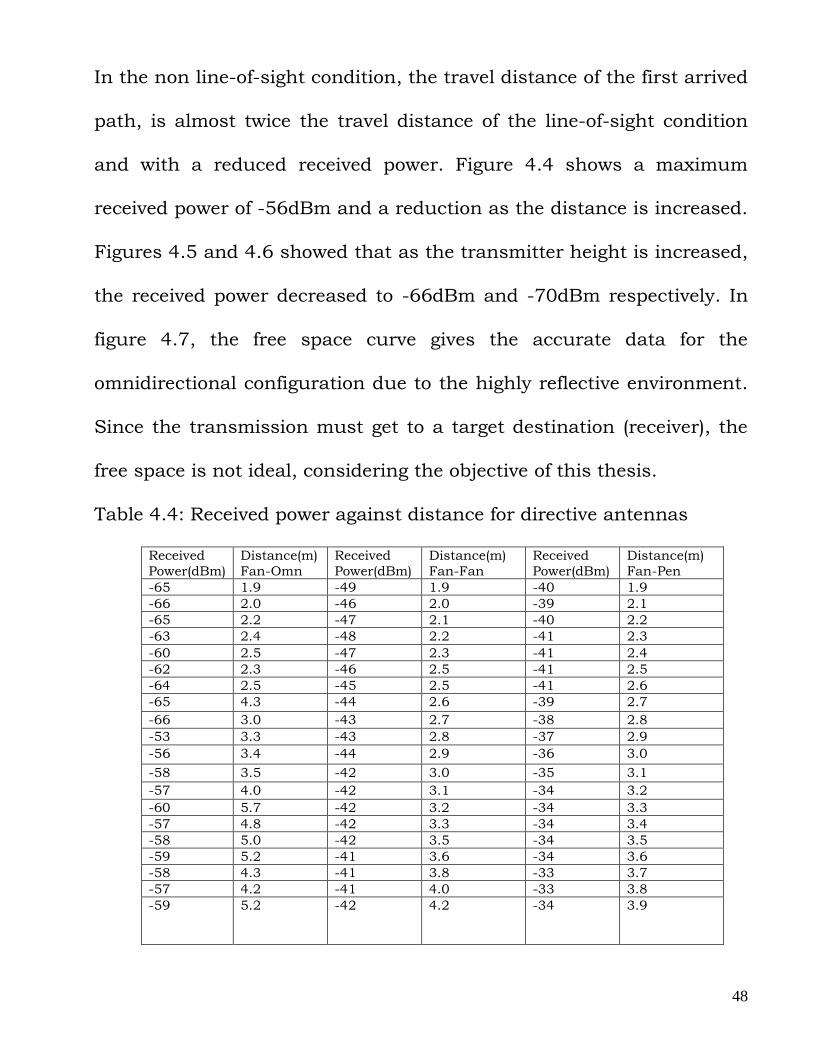
Table 4.4: Received power against distance for directive antennas

Received

Power(dBm)

Distance(m)

Fan-Omn

Received

Power(dBm)

Distance(m)

Fan-Fan

Received

Power(dBm)

Distance(m)

Fan-Pen

-65 1.9 -49 1.9 -40 1.9

-66 2.0 -46 2.0 -39 2.1

-65 2.2 -47 2.1 -40 2.2

-63 2.4 -48 2.2 -41 2.3

-60 2.5 -47 2.3 -41 2.4

-62 2.3 -46 2.5 -41 2.5

-64 2.5 -45 2.5 -41 2.6

-65 4.3 -44 2.6 -39 2.7

-66 3.0 -43 2.7 -38 2.8

-53 3.3 -43 2.8 -37 2.9

-56 3.4 -44 2.9 -36 3.0

-58 3.5 -42 3.0 -35 3.1

-57 4.0 -42 3.1 -34 3.2

-60 5.7 -42 3.2 -34 3.3

-57 4.8 -42 3.3 -34 3.4

-58 5.0 -42 3.5 -34 3.5

-59 5.2 -41 3.6 -34 3.6

-58 4.3 -41 3.8 -33 3.7

-57 4.2 -41 4.0 -33 3.8

-59 5.2 -42

4.2 -34 3.9

49

Figure 4.8: The received power over the travel distance of the first arrived path for the Fan-Omn antennas.

1.5 2 2.5 3 3.5 4 4.5 5 5.5 6-66

-64

-62

-60

-58

-56

-54

-52

Travel distance of the first arrived path for the directive antenna(m)

Receiv

ed P

ow

er(

dB

m)

Received power against TX/RX distance for Fan-Omn antennas

50

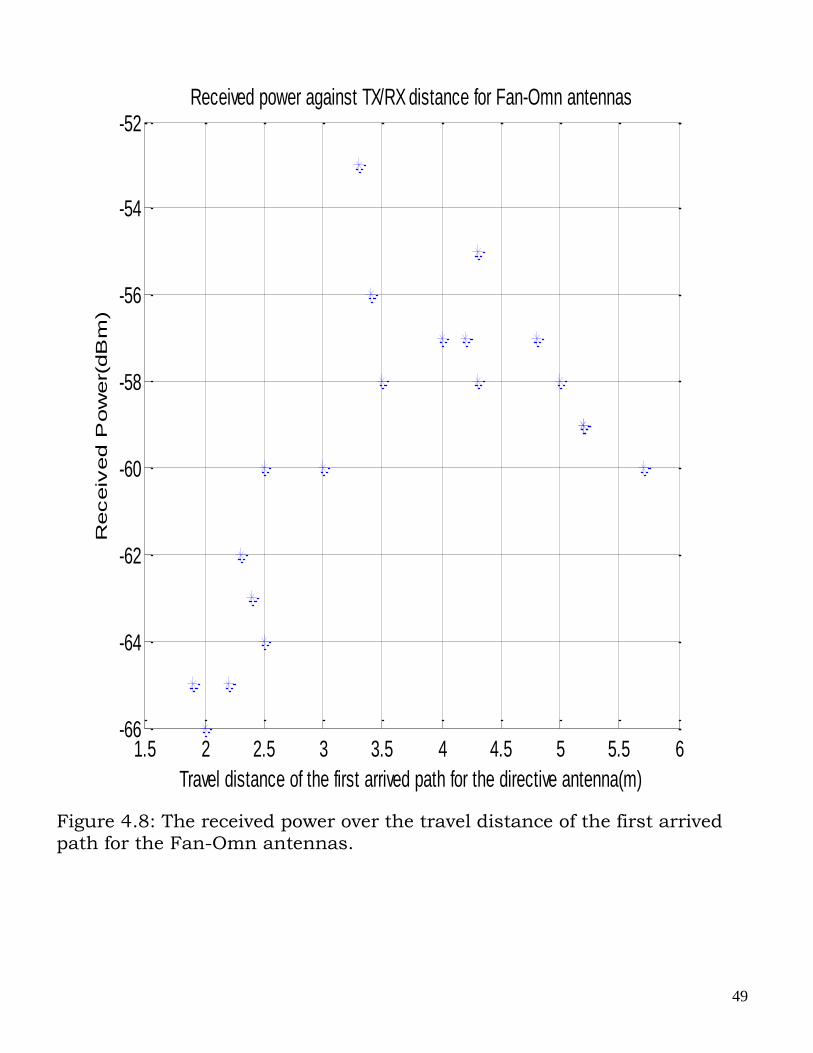
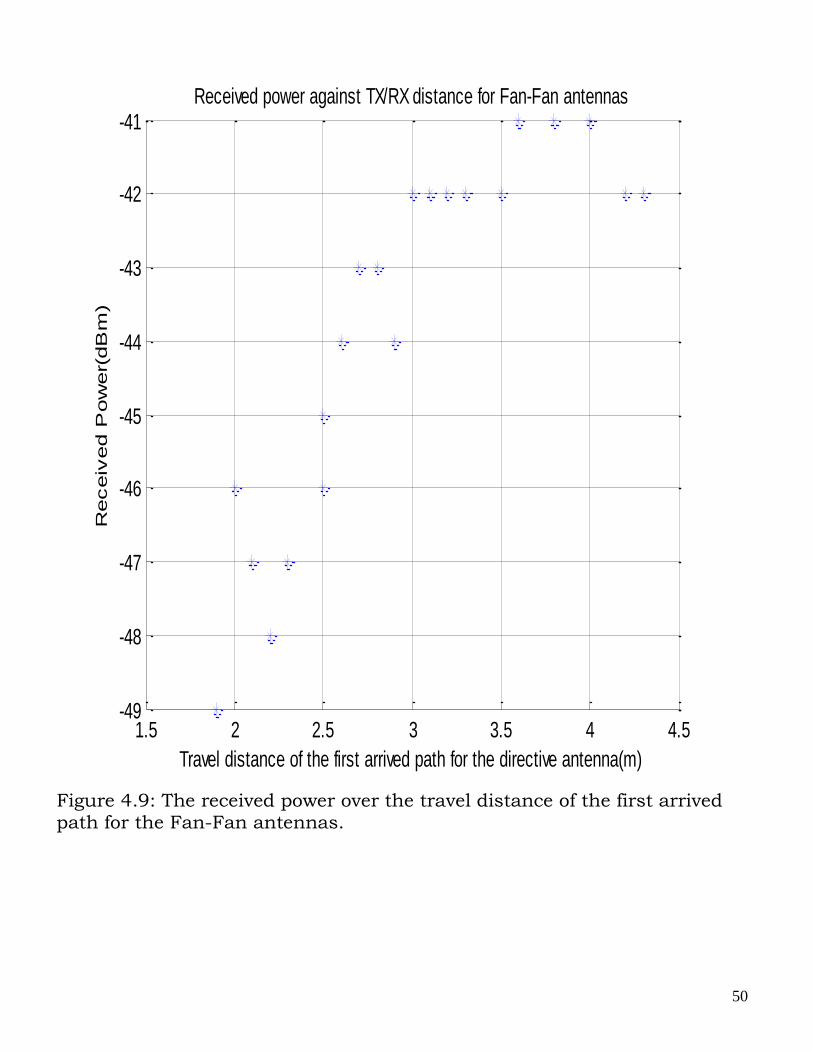
Figure 4.9: The received power over the travel distance of the first arrived path for the Fan-Fan antennas.

1.5 2 2.5 3 3.5 4 4.5-49

-48

-47

-46

-45

-44

-43

-42

-41

Travel distance of the first arrived path for the directive antenna(m)

Receiv

ed P

ow

er(

dB

m)

Received power against TX/RX distance for Fan-Fan antennas

51

Figure 4.10: The received power over the travel distance of the first arrived path for the Fan-Pen antennas.

Table 4.5: Received power against distance for directive antennas with 35°

Received Power(dBm)

-53 -51 -50 -53 -53 -54 -53 -54 -50 -49 -48 -48 -48 -49 -48 -49 -47 -47 -47 -47

Distance(m)

Fan-Fan 35°

1.9 2.0 2.1 2.2 2.3 2.4 2.5 2.6 2.7 2.8 2.9 3.1 3.2 3.3 3.4 3.5 3.6 3.7 4.2 4.4

Received

Power(dBm)

-66 -67 -67 -68 -65 -64 -64 -65 -65 -65 -65 -66 -66 -67 -65 -66 -66 -65 -66 -65

Distance(m)

Fan-Pen 35°

1.9 2.0 2.1 2.2 2.3 2.4 2.5 2.6 2.7 2.9 3.0 3.2 3.3 3.5 3.6 3.7 4.2 4.3 4.4 4.5

1.5 2 2.5 3 3.5 4-41

-40

-39

-38

-37

-36

-35

-34

-33

Travel distance of the first arrived path for the directive antenna(m)

Receiv

ed P

ow

er(

dB

m)

Received power against TX/RX distance for Fan-Pen antennas

52

Figure 4.11: The received power over the travel distance of the first arrived path for the Fan-Fan antennas with 35° misalignment.

1.5 2 2.5 3 3.5 4 4.5-54

-53

-52

-51

-50

-49

-48

-47

Travel distance of the first arrived path for directive antenna(m)

Receiv

ed P

ow

er(

dB

m)

Received power against TX/RX distance for Fan-Fan 35(degree) deviation

53

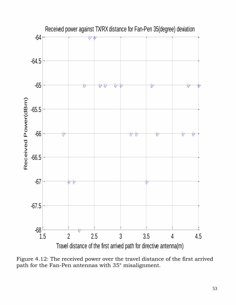
Figure 4.12: The received power over the travel distance of the first arrived path for the Fan-Pen antennas with 35° misalignment.

1.5 2 2.5 3 3.5 4 4.5-68

-67.5

-67

-66.5

-66

-65.5

-65

-64.5

-64

Travel distance of the first arrived path for directive antenna(m)

Receiv

ed P

ow

er(dB

m)

Received power against TX/RX distance for Fan-Pen 35(degree) deviation

54

Figure 4.8 has a maximum received power of -53dBm and

compared to the directive antenna configuration in figures 4.9 to 4.12,

the power level is much higher and the scattered points strongly

assume a definite path except those close to the transmitter that are

very sensitive to the unintentional beam pointing errors. This is due to

the use of an omnidirectional antenna as the receiver. When the

receiver beams are misaligned intentionally by ±35˚ over the boresight,

the received power by the fan-pen configuration (figure 4.10) will drop

about 27dB due to narrower antenna beam, compared to the 5dB drop

by the fan-fan antennas as shown in figure 4.9. From observations, the

35˚ misalignment is about half the beamwidth of the fan-beam antenna

and thus the direct path is still within the sight. It appears that the

loss exponents are much smaller than the free-space exponent for the

omn-omn configurations but approximately equal to 2 for the directive

antenna loss exponent.

55

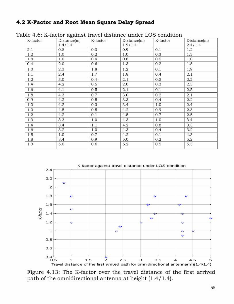
4.2 K-Factor and Root Mean Square Delay Spread Table 4.6: K-factor against travel distance under LOS condition

K-factor Distance(m)

1.4/1.4

K-factor Distance(m)

1.9/1.4

K-factor Distance(m)

2.4/1.4

2.1 0.8 0.3 0.9 0.1 1.2

1.2 1.0 0.2 1.0 0.3 1.3

1.8 1.0 0.4 0.8 0.5 1.0

0.4 2.0 0.6 1.3 0.2 1.8

1.0 2.3 1.8 1.2 0.1 1.9

1.1 2.4 1.7 1.8 0.4 2.1

1.2 3.0 0.4 2.1 0.5 2.2

1.4 4.2 0.5 2.0 0.3 2.3

1.6 4.1 0.5 2.1 0.1 2.5

1.8 4.3 0.7 3.0 0.2 2.1

0.9 4.2 0.5 3.3 0.4 2.2

1.0 4.2 0.3 3.4 1.0 2.4

1.0 4.5 0.5 4.2 0.9 2.3

1.2 4.2 0.1 4.5 0.7 2.5

1.3 3.3 1.0 4.3 1.0 3.4

1.4 3.4 1.1 4.2 0.8 3.3

1.6 3.2 1.0 4.3 0.4 3.2

1.5 1.0 0.7 4.2 0.1 4.3

1.8 3.4 0.9 5.0 0.2 5.2

1.3 5.0 0.6 5.2 0.5 5.3

Figure 4.13: The K-factor over the travel distance of the first arrived path of the omnidirectional antenna at height (1.4/1.4).

0.5 1 1.5 2 2.5 3 3.5 4 4.5 50.4

0.6

0.8

1

1.2

1.4

1.6

1.8

2

2.2

2.4

K-fa

ctor

Travel distance of the first arrived path for omnidirectional antenna(m)(1.4/1.4)

K-factor against travel distance under LOS condition

56

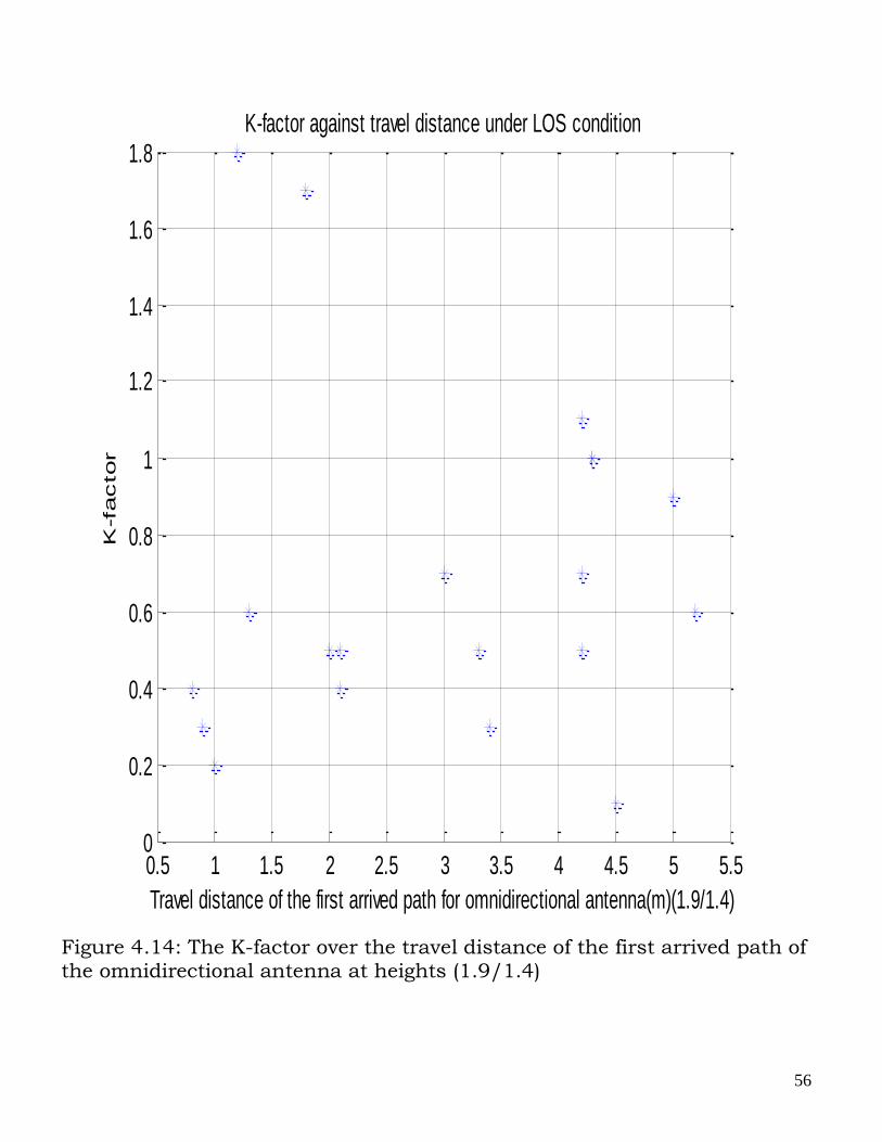
Figure 4.14: The K-factor over the travel distance of the first arrived path of the omnidirectional antenna at heights (1.9/1.4)

0.5 1 1.5 2 2.5 3 3.5 4 4.5 5 5.50

0.2

0.4

0.6

0.8

1

1.2

1.4

1.6

1.8

K-f

acto

r

Travel distance of the first arrived path for omnidirectional antenna(m)(1.9/1.4)

K-factor against travel distance under LOS condition

57

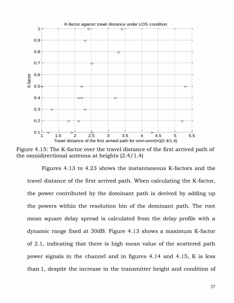
Figure 4.15: The K-factor over the travel distance of the first arrived path of the omnidirectional antenna at heights (2.4/1.4)

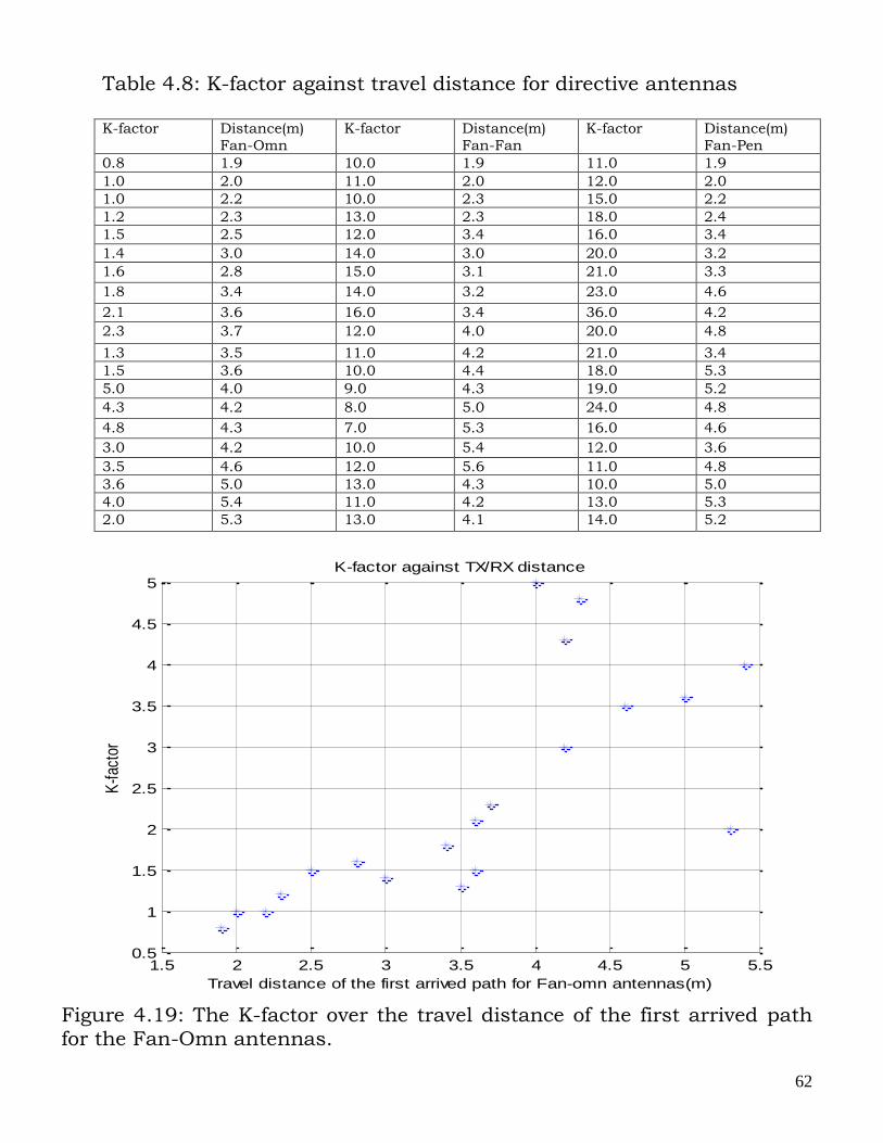
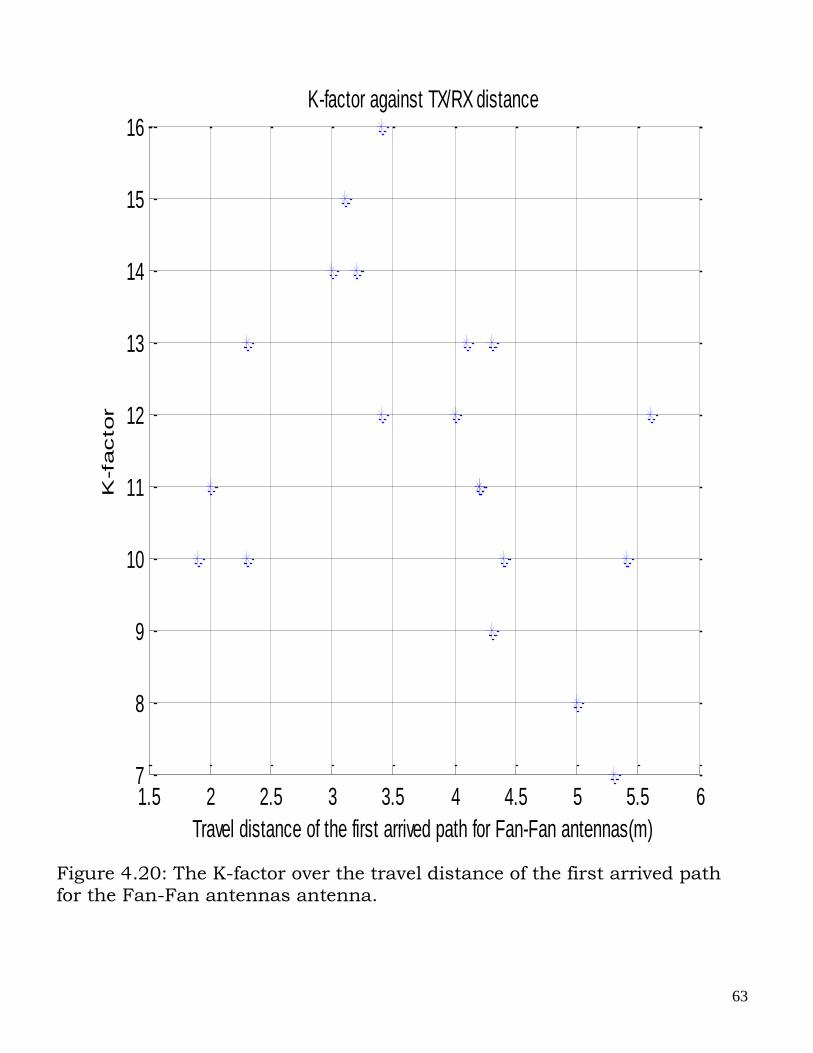
Figures 4.13 to 4.23 shows the instantaneous K-factors and the

travel distance of the first arrived path. When calculating the K-factor,

the power contributed by the dominant path is derived by adding up

the powers within the resolution bin of the dominant path. The root

mean square delay spread is calculated from the delay profile with a

dynamic range fixed at 30dB. Figure 4.13 shows a maximum K-factor

of 2.1, indicating that there is high mean value of the scattered path

power signals in the channel and in figures 4.14 and 4.15, K is less

than 1, despite the increase in the transmitter height and condition of

1 1.5 2 2.5 3 3.5 4 4.5 5 5.50.1

0.2

0.3

0.4

0.5

0.6

0.7

0.8

0.9

1K

-fac

tor

Travel distance of the first arrived path for omn-omn(m)(2.4/1.4)

K-factor against travel distance under LOS condition

58

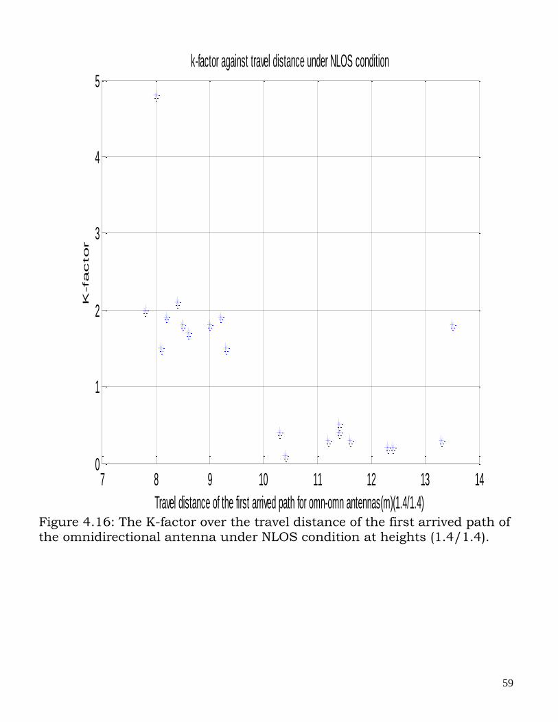
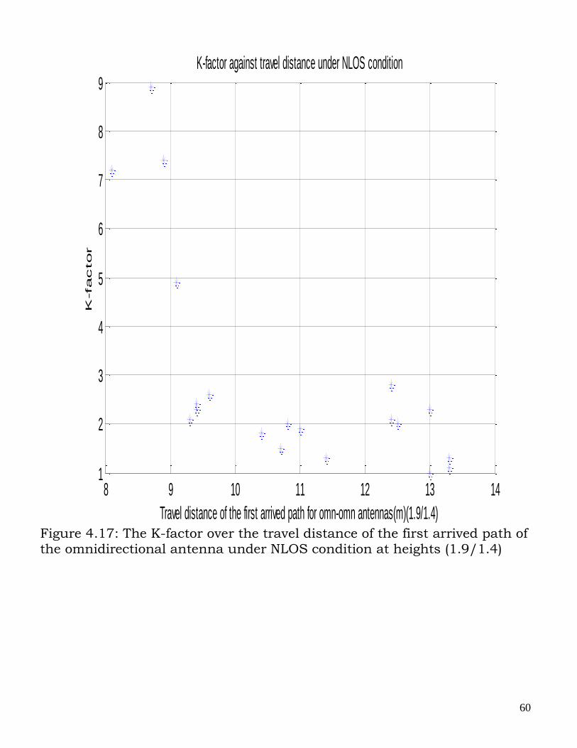
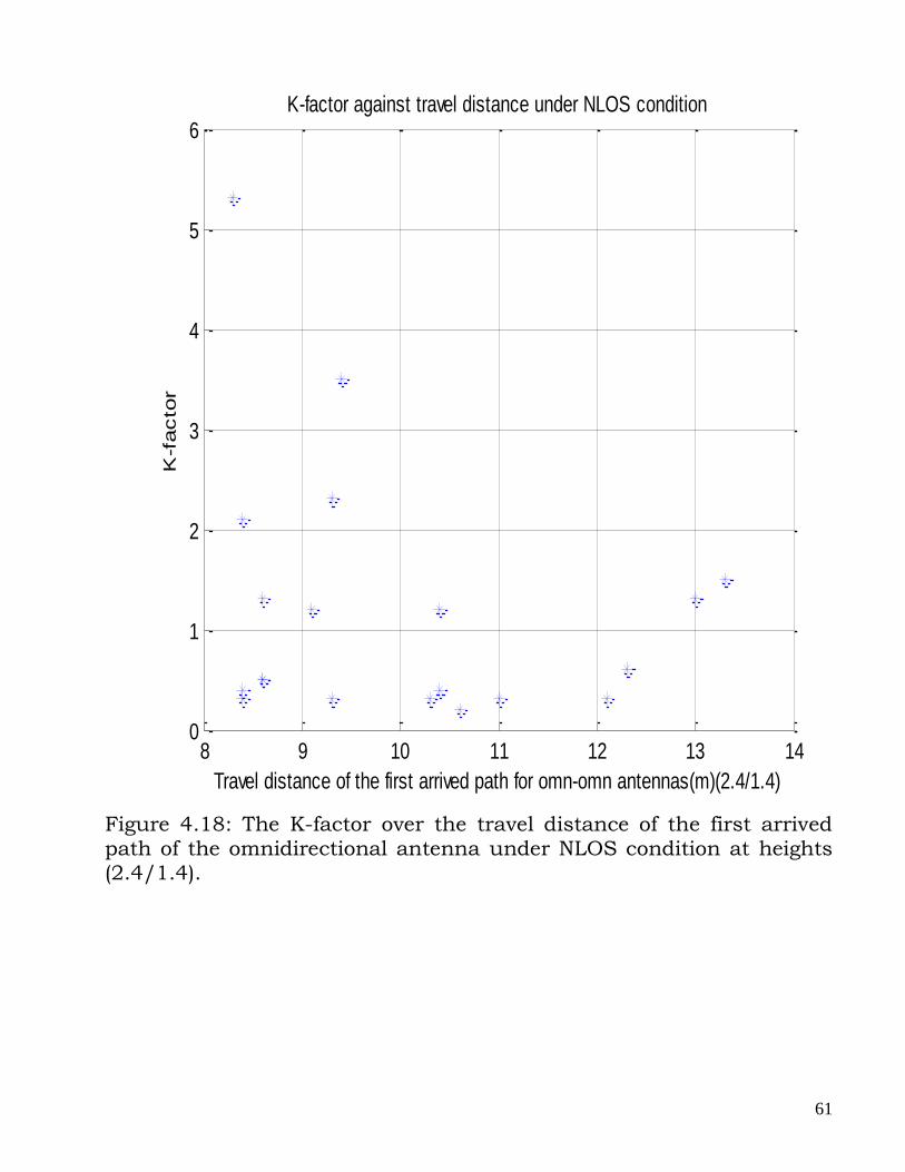
measurement. In figure 4.18, it increased to 5.4, but it cannot be said

that the channel is free from fading. In figure 4.17 below, the maximum

K-factor is 8.9, but most of the points lie between 1 and 3 indicating

that, that configuration can only be used when the travel distance is

between 8 and 9. This means that in non line of sight condition, the

receiver must be stationary else more fading will be introduced into the

communication channel.

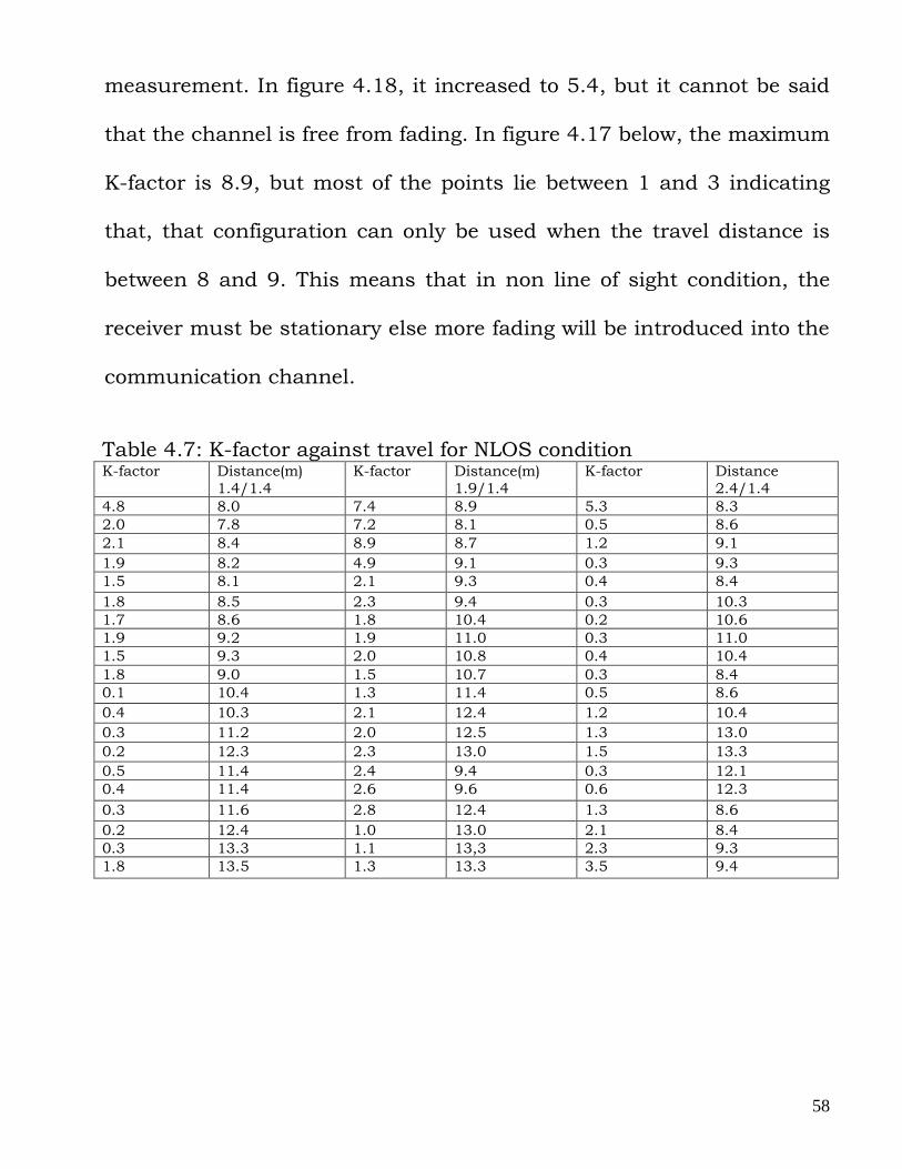
Table 4.7: K-factor against travel for NLOS condition

K-factor Distance(m)

1.4/1.4

K-factor Distance(m)

1.9/1.4

K-factor Distance

2.4/1.4

4.8 8.0 7.4 8.9 5.3 8.3

2.0 7.8 7.2 8.1 0.5 8.6

2.1 8.4 8.9 8.7 1.2 9.1

1.9 8.2 4.9 9.1 0.3 9.3

1.5 8.1 2.1 9.3 0.4 8.4

1.8 8.5 2.3 9.4 0.3 10.3

1.7 8.6 1.8 10.4 0.2 10.6

1.9 9.2 1.9 11.0 0.3 11.0

1.5 9.3 2.0 10.8 0.4 10.4

1.8 9.0 1.5 10.7 0.3 8.4

0.1 10.4 1.3 11.4 0.5 8.6

0.4 10.3 2.1 12.4 1.2 10.4

0.3 11.2 2.0 12.5 1.3 13.0

0.2 12.3 2.3 13.0 1.5 13.3

0.5 11.4 2.4 9.4 0.3 12.1

0.4 11.4 2.6 9.6 0.6 12.3

0.3 11.6 2.8 12.4 1.3 8.6

0.2 12.4 1.0 13.0 2.1 8.4

0.3 13.3 1.1 13,3 2.3 9.3

1.8 13.5 1.3 13.3 3.5 9.4

59

Figure 4.16: The K-factor over the travel distance of the first arrived path of the omnidirectional antenna under NLOS condition at heights (1.4/1.4).

7 8 9 10 11 12 13 140

1

2

3

4

5K

-factor

Travel distance of the first arrived path for omn-omn antennas(m)(1.4/1.4)

k-factor against travel distance under NLOS condition

60

Figure 4.17: The K-factor over the travel distance of the first arrived path of the omnidirectional antenna under NLOS condition at heights (1.9/1.4)

8 9 10 11 12 13 141

2

3

4

5

6

7

8

9K

-factor

Travel distance of the first arrived path for omn-omn antennas(m)(1.9/1.4)

K-factor against travel distance under NLOS condition

61

Figure 4.18: The K-factor over the travel distance of the first arrived path of the omnidirectional antenna under NLOS condition at heights (2.4/1.4).

8 9 10 11 12 13 140

1

2

3

4

5

6

K-f

acto

r

Travel distance of the first arrived path for omn-omn antennas(m)(2.4/1.4)

K-factor against travel distance under NLOS condition

62

Table 4.8: K-factor against travel distance for directive antennas

K-factor Distance(m)

Fan-Omn

K-factor Distance(m)

Fan-Fan

K-factor Distance(m)

Fan-Pen

0.8 1.9 10.0 1.9 11.0 1.9

1.0 2.0 11.0 2.0 12.0 2.0

1.0 2.2 10.0 2.3 15.0 2.2

1.2 2.3 13.0 2.3 18.0 2.4

1.5 2.5 12.0 3.4 16.0 3.4

1.4 3.0 14.0 3.0 20.0 3.2

1.6 2.8 15.0 3.1 21.0 3.3

1.8 3.4 14.0 3.2 23.0 4.6

2.1 3.6 16.0 3.4 36.0 4.2

2.3 3.7 12.0 4.0 20.0 4.8

1.3 3.5 11.0 4.2 21.0 3.4

1.5 3.6 10.0 4.4 18.0 5.3

5.0 4.0 9.0 4.3 19.0 5.2

4.3 4.2 8.0 5.0 24.0 4.8

4.8 4.3 7.0 5.3 16.0 4.6

3.0 4.2 10.0 5.4 12.0 3.6

3.5 4.6 12.0 5.6 11.0 4.8

3.6 5.0 13.0 4.3 10.0 5.0

4.0 5.4 11.0 4.2 13.0 5.3

2.0 5.3 13.0 4.1 14.0 5.2

Figure 4.19: The K-factor over the travel distance of the first arrived path for the Fan-Omn antennas.

1.5 2 2.5 3 3.5 4 4.5 5 5.50.5

1

1.5

2

2.5

3

3.5

4

4.5

5

Travel distance of the first arrived path for Fan-omn antennas(m)

K-f

acto

r

K-factor against TX/RX distance

63

Figure 4.20: The K-factor over the travel distance of the first arrived path for the Fan-Fan antennas antenna.

1.5 2 2.5 3 3.5 4 4.5 5 5.5 67

8

9

10

11

12

13

14

15

16

Travel distance of the first arrived path for Fan-Fan antennas(m)

K-f

acto

rK-factor against TX/RX distance

64

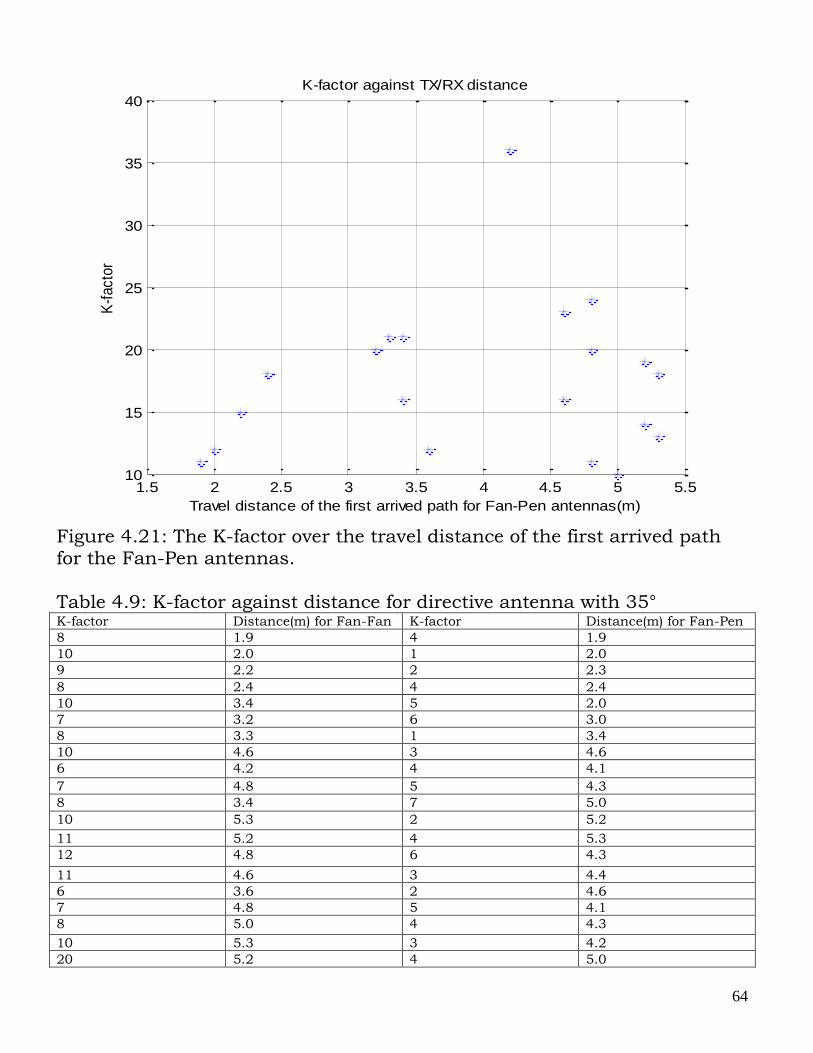
Figure 4.21: The K-factor over the travel distance of the first arrived path for the Fan-Pen antennas. Table 4.9: K-factor against distance for directive antenna with 35° K-factor Distance(m) for Fan-Fan K-factor Distance(m) for Fan-Pen

8 1.9 4 1.9

10 2.0 1 2.0

9 2.2 2 2.3

8 2.4 4 2.4

10 3.4 5 2.0

7 3.2 6 3.0

8 3.3 1 3.4

10 4.6 3 4.6

6 4.2 4 4.1

7 4.8 5 4.3

8 3.4 7 5.0

10 5.3 2 5.2

11 5.2 4 5.3

12 4.8 6 4.3

11 4.6 3 4.4

6 3.6 2 4.6

7 4.8 5 4.1

8 5.0 4 4.3

10 5.3 3 4.2

20 5.2 4 5.0

1.5 2 2.5 3 3.5 4 4.5 5 5.510

15

20

25

30

35

40

Travel distance of the first arrived path for Fan-Pen antennas(m)

K-f

acto

r

K-factor against TX/RX distance

65

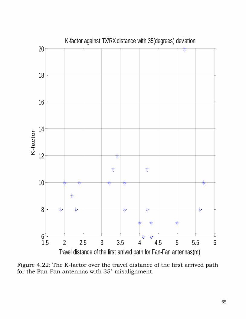
Figure 4.22: The K-factor over the travel distance of the first arrived path for the Fan-Fan antennas with 35° misalignment.

1.5 2 2.5 3 3.5 4 4.5 5 5.5 66

8

10

12

14

16

18

20

Travel distance of the first arrived path for Fan-Fan antennas(m)

K-f

acto

r

K-factor against TX/RX distance with 35(degrees) deviation

66

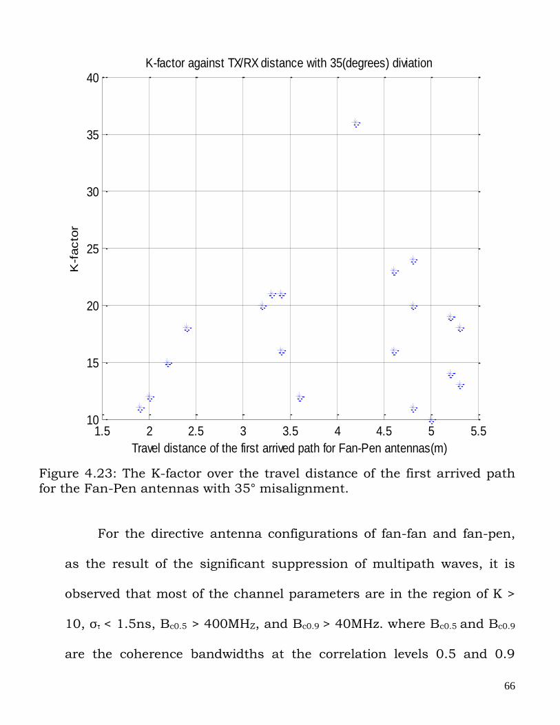
Figure 4.23: The K-factor over the travel distance of the first arrived path for the Fan-Pen antennas with 35° misalignment.

For the directive antenna configurations of fan-fan and fan-pen,

as the result of the significant suppression of multipath waves, it is

observed that most of the channel parameters are in the region of K >

10, σ < 1.5ns, Bc0.5 > 400MHZ, and Bc0.9 > 40MHz. where Bc0.5 and Bc0.9

are the coherence bandwidths at the correlation levels 0.5 and 0.9

1.5 2 2.5 3 3.5 4 4.5 5 5.510

15

20

25

30

35

40

Travel distance of the first arrived path for Fan-Pen antennas(m)

K-f

acto

rK-factor against TX/RX distance with 35(degrees) diviation

67

respectively, the mean values are listed in table 4.15. The mean values

are obtained by taking the various points of each of the parameters

obtained, and can be computed using the formular below.

(4.1)

where N is the total number of values of each parameter, is the mean

value of each parameter, is the various values of the parameters from

i to N.

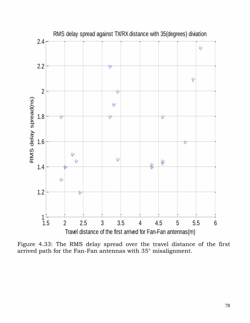
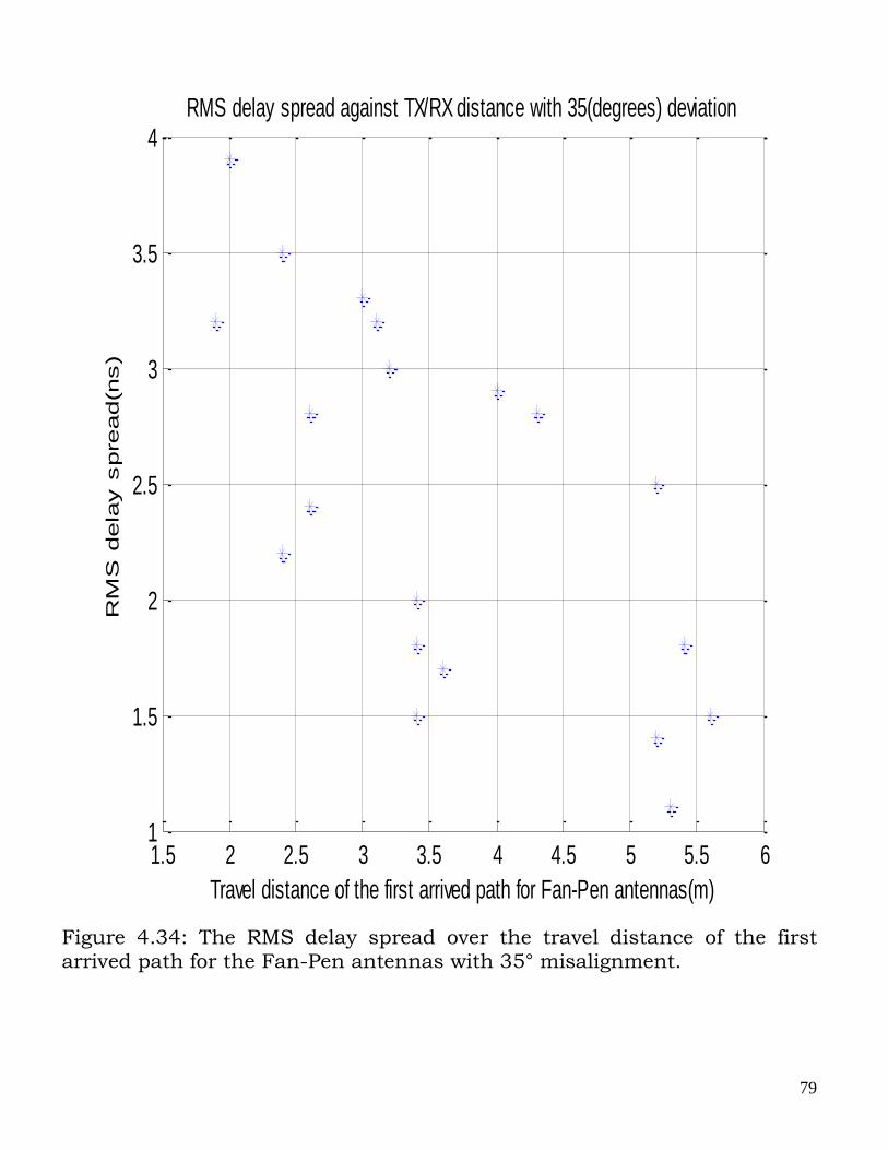
When the transmitter and receiver beams are not pointing to each

other, the beam-pointing errors, for instance the 35˚ -misalignment for

the Fan-Pen configuration can seriously worsen the channel condition

in terms of large root mean square delay spreads (RDSs), and the

enormous drop of received powers, K-factors and coherence bandwidth.

This implies that channel configurations with wider beams are less

sensitive to beam-pointing errors. That means, the width of the beam

has to be properly designed to prevent an enormous drop of channel

quality caused by beam-pointing errors. In practice, multiple antennas

can be deployed and beamforming algorithms will be used to achieve

higher gain and suppress multipath effect by steering the main beam

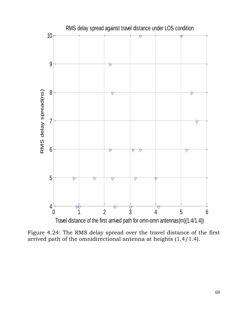
to the direction of the strongest path. Figures 4.24 to 4.34 are the root-

mean-square delay spread over the distance of the first arrived path for

the omnidirectional antenna and directive antennas.

68

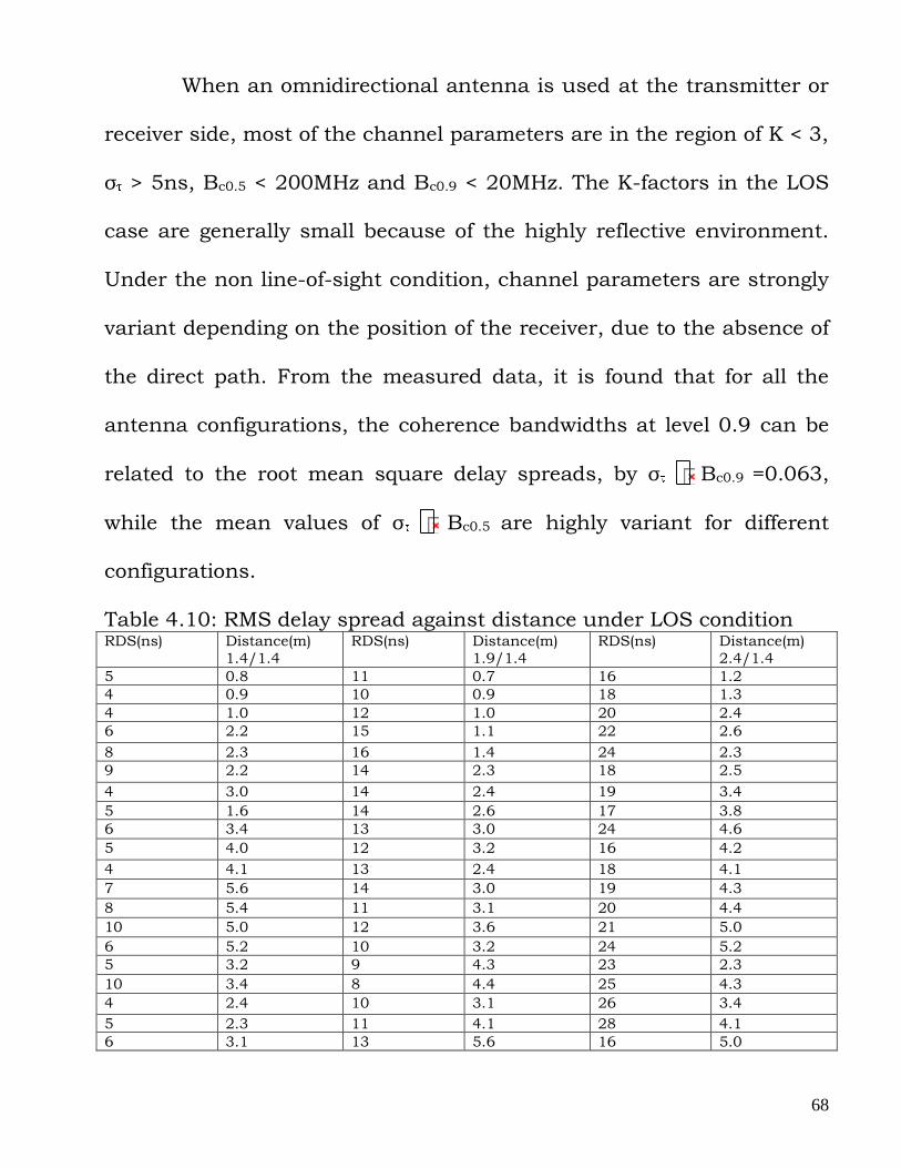
When an omnidirectional antenna is used at the transmitter or

receiver side, most of the channel parameters are in the region of K < 3,

σ > 5ns, Bc0.5 < 200MHz and Bc0.9 < 20MHz. The K-factors in the LOS

case are generally small because of the highly reflective environment.

Under the non line-of-sight condition, channel parameters are strongly

variant depending on the position of the receiver, due to the absence of

the direct path. From the measured data, it is found that for all the

antenna configurations, the coherence bandwidths at level 0.9 can be

related to the root mean square delay spreads, by σ Bc0.9 =0.063,

while the mean values of σ Bc0.5 are highly variant for different

configurations.

Table 4.10: RMS delay spread against distance under LOS condition RDS(ns) Distance(m)

1.4/1.4

RDS(ns) Distance(m)

1.9/1.4

RDS(ns) Distance(m)

2.4/1.4

5 0.8 11 0.7 16 1.2

4 0.9 10 0.9 18 1.3

4 1.0 12 1.0 20 2.4

6 2.2 15 1.1 22 2.6

8 2.3 16 1.4 24 2.3

9 2.2 14 2.3 18 2.5

4 3.0 14 2.4 19 3.4

5 1.6 14 2.6 17 3.8

6 3.4 13 3.0 24 4.6

5 4.0 12 3.2 16 4.2

4 4.1 13 2.4 18 4.1

7 5.6 14 3.0 19 4.3

8 5.4 11 3.1 20 4.4

10 5.0 12 3.6 21 5.0

6 5.2 10 3.2 24 5.2

5 3.2 9 4.3 23 2.3

10 3.4 8 4.4 25 4.3

4 2.4 10 3.1 26 3.4

5 2.3 11 4.1 28 4.1

6 3.1 13 5.6 16 5.0

69

Figure 4.24: The RMS delay spread over the travel distance of the first arrived path of the omnidirectional antenna at heights (1.4/1.4).

0 1 2 3 4 5 64

5

6

7

8

9

10

Travel distance of the first arrived path for omn-omn antennas(m)(1.4/1.4))

RM

S d

ela

y s

pre

ad(n

s)

RMS delay spread against travel distance under LOS condition

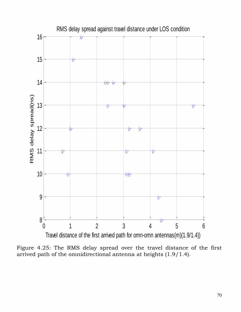
70

Figure 4.25: The RMS delay spread over the travel distance of the first arrived path of the omnidirectional antenna at heights (1.9/1.4).

0 1 2 3 4 5 68

9

10

11

12

13

14

15

16

Travel distance of the first arrived path for omn-omn antennas(m)(1.9/1.4))

RM

S d

ela

y s

pre

ad(n

s)

RMS delay spread against travel distance under LOS condition

71

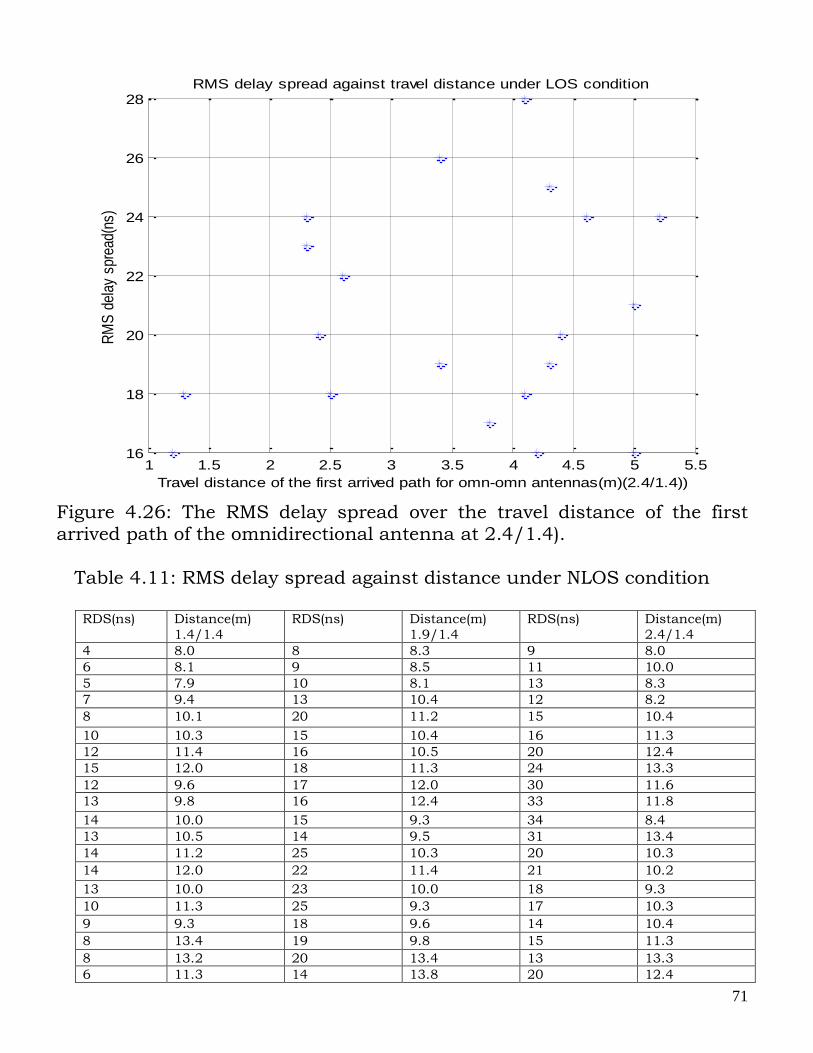
Figure 4.26: The RMS delay spread over the travel distance of the first arrived path of the omnidirectional antenna at 2.4/1.4). Table 4.11: RMS delay spread against distance under NLOS condition

RDS(ns) Distance(m)

1.4/1.4

RDS(ns) Distance(m)

1.9/1.4

RDS(ns) Distance(m)

2.4/1.4

4 8.0 8 8.3 9 8.0

6 8.1 9 8.5 11 10.0

5 7.9 10 8.1 13 8.3

7 9.4 13 10.4 12 8.2

8 10.1 20 11.2 15 10.4

10 10.3 15 10.4 16 11.3

12 11.4 16 10.5 20 12.4

15 12.0 18 11.3 24 13.3

12 9.6 17 12.0 30 11.6

13 9.8 16 12.4 33 11.8

14 10.0 15 9.3 34 8.4

13 10.5 14 9.5 31 13.4

14 11.2 25 10.3 20 10.3

14 12.0 22 11.4 21 10.2

13 10.0 23 10.0 18 9.3

10 11.3 25 9.3 17 10.3

9 9.3 18 9.6 14 10.4

8 13.4 19 9.8 15 11.3

8 13.2 20 13.4 13 13.3

6 11.3 14 13.8 20 12.4

1 1.5 2 2.5 3 3.5 4 4.5 5 5.516

18

20

22

24

26

28

Travel distance of the first arrived path for omn-omn antennas(m)(2.4/1.4))

RM

S d

elay

spr

ead(

ns)

RMS delay spread against travel distance under LOS condition

72

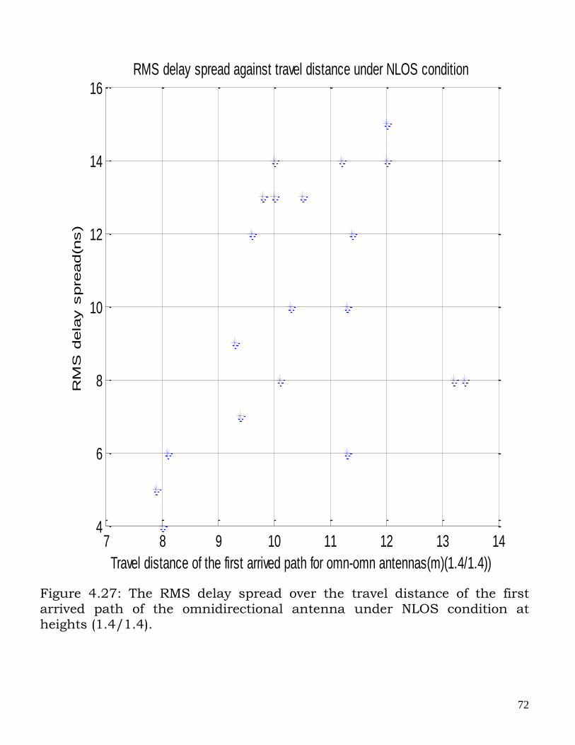
Figure 4.27: The RMS delay spread over the travel distance of the first arrived path of the omnidirectional antenna under NLOS condition at heights (1.4/1.4).

7 8 9 10 11 12 13 144

6

8

10

12

14

16

Travel distance of the first arrived path for omn-omn antennas(m)(1.4/1.4))

RM

S d

ela

y s

pre

ad(n

s)

RMS delay spread against travel distance under NLOS condition

73

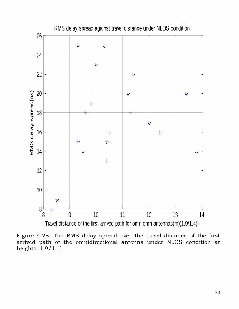
Figure 4.28: The RMS delay spread over the travel distance of the first arrived path of the omnidirectional antenna under NLOS condition at heights (1.9/1.4)

8 9 10 11 12 13 148

10

12

14

16

18

20

22

24

26

Travel distance of the first arrived path for omn-omn antennas(m)(1.9/1.4))

RM

S d

ela

y s

pre

ad(n

s)

RMS delay spread against travel distance under NLOS condition

74

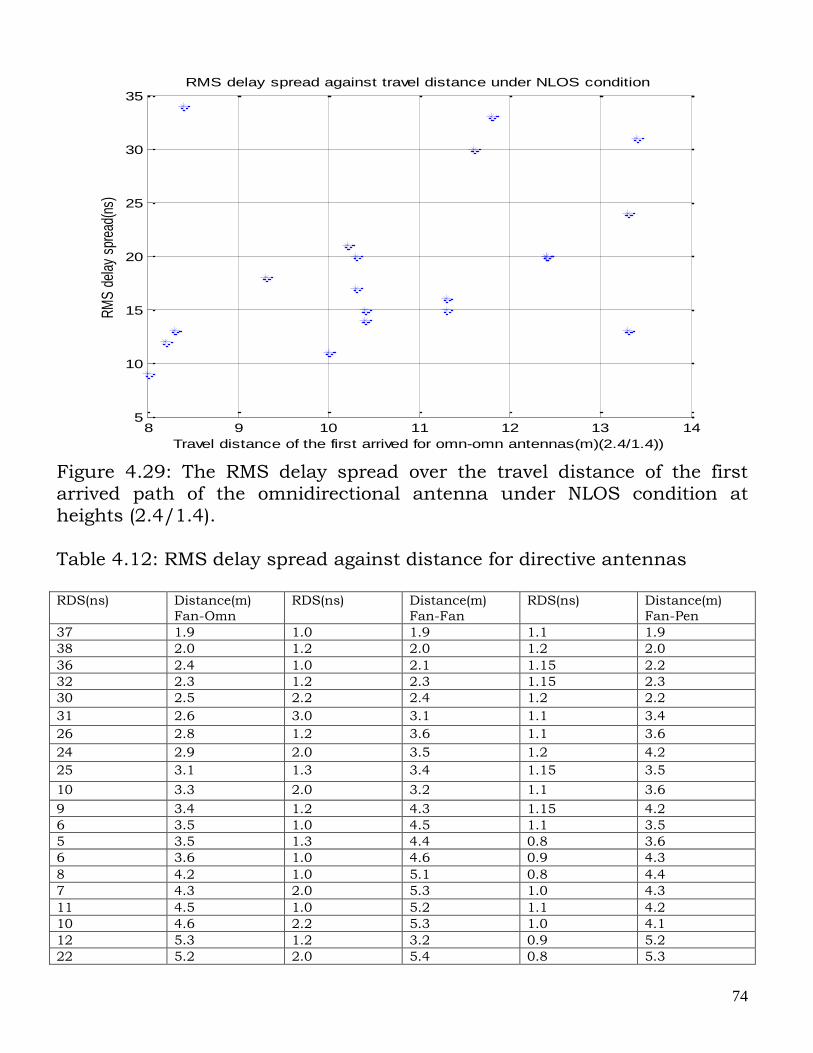
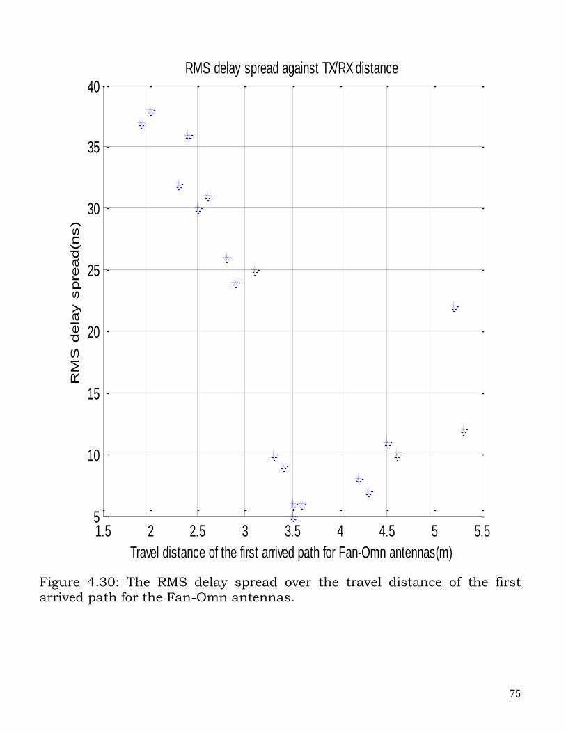
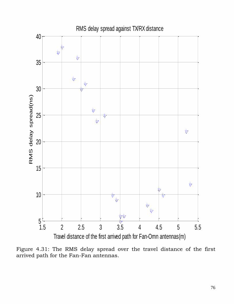
Figure 4.29: The RMS delay spread over the travel distance of the first arrived path of the omnidirectional antenna under NLOS condition at heights (2.4/1.4). Table 4.12: RMS delay spread against distance for directive antennas RDS(ns) Distance(m)

Fan-Omn

RDS(ns) Distance(m)

Fan-Fan

RDS(ns) Distance(m)

Fan-Pen

37 1.9 1.0 1.9 1.1 1.9

38 2.0 1.2 2.0 1.2 2.0

36 2.4 1.0 2.1 1.15 2.2

32 2.3 1.2 2.3 1.15 2.3

30 2.5 2.2 2.4 1.2 2.2

31 2.6 3.0 3.1 1.1 3.4

26 2.8 1.2 3.6 1.1 3.6

24 2.9 2.0 3.5 1.2 4.2

25 3.1 1.3 3.4 1.15 3.5

10 3.3 2.0 3.2 1.1 3.6

9 3.4 1.2 4.3 1.15 4.2

6 3.5 1.0 4.5 1.1 3.5

5 3.5 1.3 4.4 0.8 3.6

6 3.6 1.0 4.6 0.9 4.3

8 4.2 1.0 5.1 0.8 4.4

7 4.3 2.0 5.3 1.0 4.3

11 4.5 1.0 5.2 1.1 4.2

10 4.6 2.2 5.3 1.0 4.1

12 5.3 1.2 3.2 0.9 5.2

22 5.2 2.0 5.4 0.8 5.3

8 9 10 11 12 13 145

10

15

20

25

30

35

Travel distance of the first arrived for omn-omn antennas(m)(2.4/1.4))

RM

S d

elay

spr

ead(

ns)

RMS delay spread against travel distance under NLOS condition

75

Figure 4.30: The RMS delay spread over the travel distance of the first arrived path for the Fan-Omn antennas.

1.5 2 2.5 3 3.5 4 4.5 5 5.55

10

15

20

25

30

35

40

Travel distance of the first arrived path for Fan-Omn antennas(m)

RM

S d

ela

y s

pre

ad(n

s)

RMS delay spread against TX/RX distance

76

Figure 4.31: The RMS delay spread over the travel distance of the first arrived path for the Fan-Fan antennas.

1.5 2 2.5 3 3.5 4 4.5 5 5.55

10

15

20

25

30

35

40

Travel distance of the first arrived path for Fan-Omn antennas(m)

RM

S d

ela

y s

pre

ad(n

s)

RMS delay spread against TX/RX distance

77

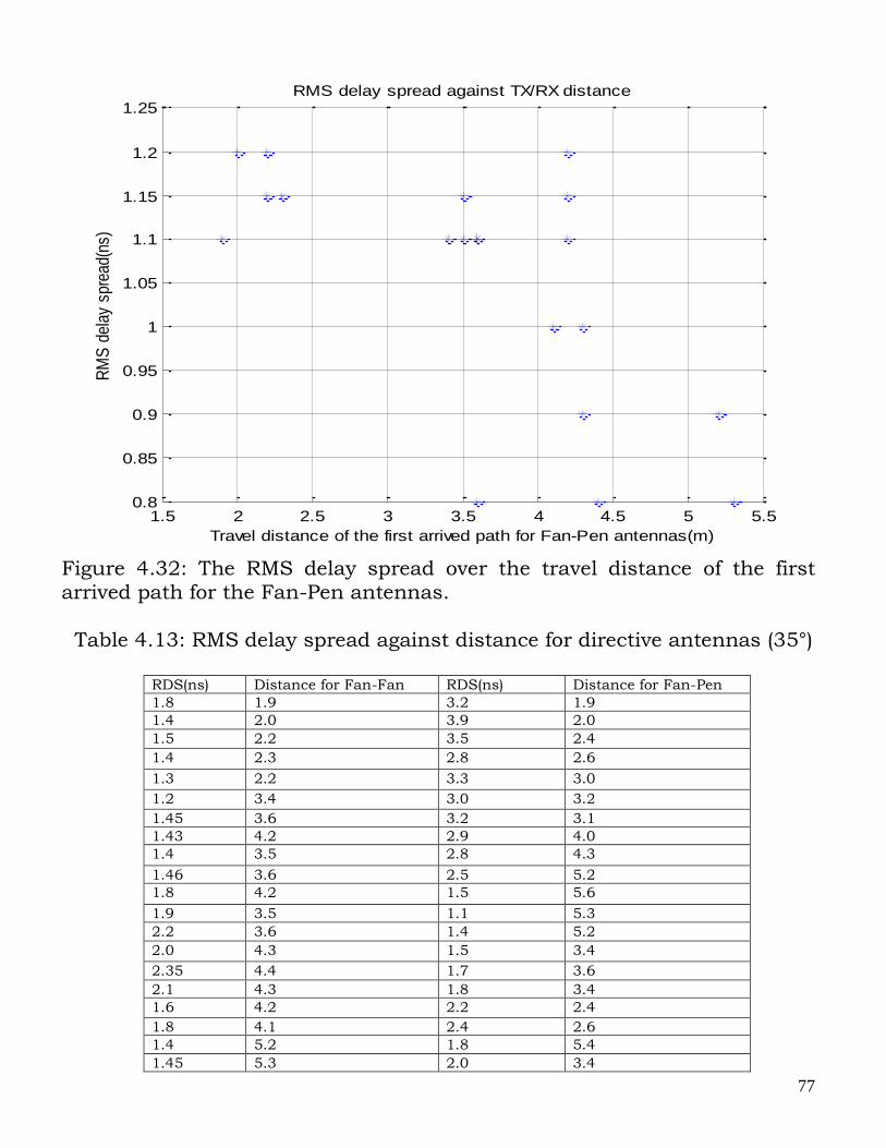
Figure 4.32: The RMS delay spread over the travel distance of the first arrived path for the Fan-Pen antennas. Table 4.13: RMS delay spread against distance for directive antennas (35°)

RDS(ns) Distance for Fan-Fan RDS(ns) Distance for Fan-Pen

1.8 1.9 3.2 1.9

1.4 2.0 3.9 2.0

1.5 2.2 3.5 2.4

1.4 2.3 2.8 2.6

1.3 2.2 3.3 3.0

1.2 3.4 3.0 3.2

1.45 3.6 3.2 3.1

1.43 4.2 2.9 4.0

1.4 3.5 2.8 4.3

1.46 3.6 2.5 5.2

1.8 4.2 1.5 5.6

1.9 3.5 1.1 5.3

2.2 3.6 1.4 5.2

2.0 4.3 1.5 3.4

2.35 4.4 1.7 3.6

2.1 4.3 1.8 3.4

1.6 4.2 2.2 2.4

1.8 4.1 2.4 2.6

1.4 5.2 1.8 5.4

1.45 5.3 2.0 3.4

1.5 2 2.5 3 3.5 4 4.5 5 5.50.8

0.85

0.9

0.95

1

1.05

1.1

1.15

1.2

1.25

Travel distance of the first arrived path for Fan-Pen antennas(m)

RM

S d

elay

spr

ead(

ns)

RMS delay spread against TX/RX distance

78

Figure 4.33: The RMS delay spread over the travel distance of the first arrived path for the Fan-Fan antennas with 35° misalignment.

1.5 2 2.5 3 3.5 4 4.5 5 5.5 61

1.2

1.4

1.6

1.8

2

2.2

2.4

Travel distance of the first arrived for Fan-Fan antennas(m)

RM

S d

ela

y s

pre

ad(n

s)

RMS delay spread against TX/RX distance with 35(degrees) diviation

79

Figure 4.34: The RMS delay spread over the travel distance of the first arrived path for the Fan-Pen antennas with 35° misalignment.

1.5 2 2.5 3 3.5 4 4.5 5 5.5 61

1.5

2

2.5

3

3.5

4

Travel distance of the first arrived path for Fan-Pen antennas(m)

RM

S d

ela

y s

pre

ad(n

s)

RMS delay spread against TX/RX distance with 35(degrees) deviation

80

4.3 Power Delay Profile

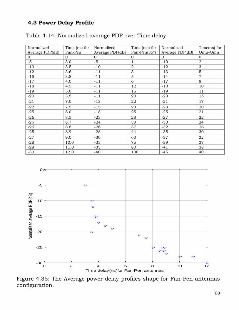
Table 4.14: Normalized average PDP over Time delay

Normalized

Average PDP(dB)

Time (ns) for

Fan-Pen

Normalized

Average PDP(dB)

Time (ns)) for

Fan-Pen(35°)

Normalized

Average PDP(dB)

Time(ns) for

Omn-Omn

0 0 0 0 0 0

-5 3.0 -5 1 -10 2

-10 3.5 -10 2 -12 3

-12 3.6 -11 3 -13 5

-15 3.8 -11 5 -14 7

-17 4.0 -11 6 -17 8

-18 4.5 -11 12 -18 10

-19 5.0 -11 15 -19 11

-20 3.5 -11 20 -20 15

-21 7.0 -13 22 -21 17

-22 7.5 -15 23 -23 20

-25 8.0 -18 25 -25 21

-26 8.5 -23 28 -27 22

-25 8.7 -24 33 -30 24

-26 8.8 -26 37 -32 26

-25 8.9 -28 44 -35 30

-27 9.0 -30 60 -37 32

-28 10.0 -33 75 -39 37

-28 11.0 -35 80 -41 38

-30 12.0 -40 100 -45 40

Figure 4.35: The Average power delay profiles shape for Fan-Pen antennas configuration.

0 2 4 6 8 10 12-30

-25

-20

-15

-10

-5

0

Time delay(ns)for Fan-Pen antennas

Nor

mal

ized

ave

rage

PD

P(d

B)

81

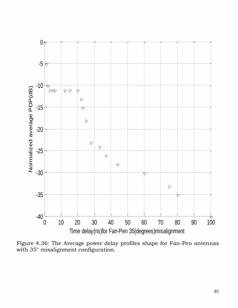
Figure 4.36: The Average power delay profiles shape for Fan-Pen antennas with 35° misalignment configuration.

0 10 20 30 40 50 60 70 80 90 100-40

-35

-30

-25

-20

-15

-10

-5

0

Time delay(ns)for Fan-Pen 35(degrees)misalignment

Norm

alized a

vera

ge P

DP

(dB

)

82

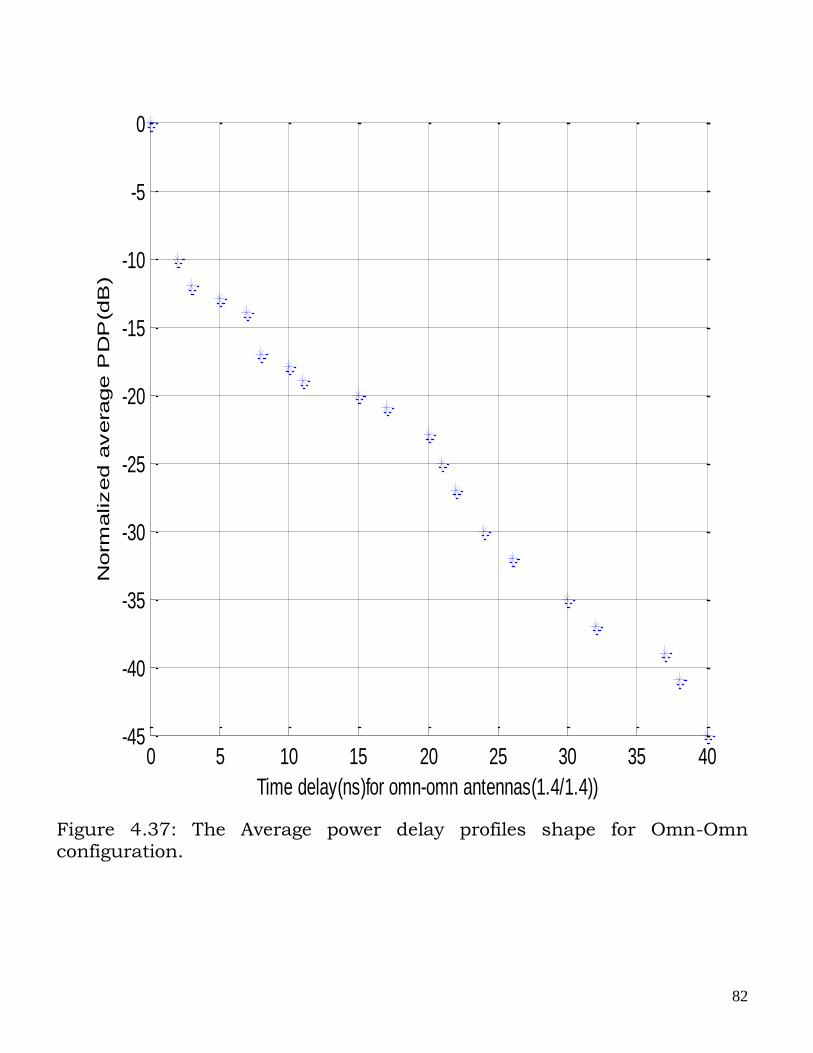
Figure 4.37: The Average power delay profiles shape for Omn-Omn configuration.

0 5 10 15 20 25 30 35 40-45

-40

-35

-30

-25

-20

-15

-10

-5

0

Time delay(ns)for omn-omn antennas(1.4/1.4))

Norm

alized a

vera

ge P

DP

(dB

)

83

Taking the average over all the measured profiles for each

configuration, each individual profile is normalized by its total received

power. From these averages, the following can be observed as shown in

the figures above.

(1) Figure 4.37 shows that when the transmitter and receiver beams are

aligned to each other under the line-of-sight condition, the normalized

average delay profile consists of a direct ray and an exponentially

decaying part.

(2) Under the non line-of-sight condition, the average delay profile will be

exponentially decaying without a constant part, due to the lower

dependency of antenna pattern and misalignment.

(3) Figure 4.36 shows that when the transmitter and receiver beams are

strongly misaligned and out of sight to each other, a constant level part

will appear before an exponentially decaying part. It can be observed

that, the average delay profile can be regarded as a function of excess

delay that consists of a direct part, a constant part and a linear

decaying part.

84

85

4.4 Maximum Excess Delays and Number of Multipath Component For the various measurement configurations, the multipath

components are recognized from the local peaks in the profile. Within

the dynamic range of 30dB of power delay profile, the maximum excess

max and the number of multipath components N are determined.

max are distributed within 10 to 170ns and so is the

values of N within 3 to 100, depending on the channel configurations.

For all the measured profiles, the number of paths per nanosecond,

max, has a mean value of 0.3 with a standard deviation of 0.06

showing that there is minimum delay using the 60GHz band.

86

CHAPTER 5

CONCLUSION

In this report, the time dispersion and frequency selectivity of

millimeter wave propagation at 60GHz channels with various antenna

configurations were based on extensive channel measurements in Line-

of-sight and non line-of-sight environments. Statistical channel

parameters were obtained from the measurement and compared, which

showed that the power level of the directive antenna configuration is

much higher and the loss exponents are much smaller than the free-

space for omn-omn configuration. The measurement of the width of the

delay power spectrum known as RMS delay spread and power delay

profiles were retrieved based on a simple profile model.

5.1 Conclusion

For the considered environments and antenna configurations, the

following conclusions can be drawn.

(1) The transmitter and receiver antenna beams have to be properly

aligned within the sight of each other, else the beam-pointing errors

will cause an enormous drop in the channel quality. The wider beam

antennas are less sensitive for beam-pointing errors, which indicates

that a proper beamwidth has to be designed in practice.

87

(2) To increase the signal coverage and performance in the NLOS area, it

is preferable to apply directive antennas.

(3) When an omnidirectional antenna is used at the transmitter or

receiver side in a LOS case, the channel parameters are generally small

because of the reflective environment.

(4) The measurement results have shown that the use of high gain

antenna can significantly reduce the delay spread of the distributed

wireless communication system channel when the transmitter and

receiver antennas are aligned.

5.2 Recommendation

Based on the above analysis and results obtained, it can be

observed that millimeter wave propagation has the potentials to provide

the next generation multigigabit wireless communication system.

Further research work could be aimed at understanding the link

budget, the effects of rain-induced bistatic scattering, and the effects of

atmospheric oxygen, humidity and fog in millimeter wave propagation.

88

REFERENCES

Balanis C.A. (1997): Antenna Theory: Analysis and Design, John Wiley & Sons, New York, NY, USA, 2nd edition.

Chong C.C. and Yong S.K. (2007): An overview of multigigabit wireless through millimeter wave technology: potentials and technical challenges, EURASIP Journal, 2007 (2): 3 – 6.

Kvicera V. and Grabner M. (2007): Rain Attenuation at 58 GHz: Prediction versus Long-Term Trial Results, EURASIP Journal, 2007 (6): 3-6.

Lim C.P, Lee, M., Burkholder R.J., Volakis J.L., Marhefka, R.J. (2007): 60 GHz indoor propagation studies for wireless communication based on Ray-tracing method, EURASIP Journal, 2007 (4): 2 – 3.

Mohammadi A., Shayegh Abdipour, A. and Mirzavand R. (2007): Direct Conversion EHM transceivers Design for millimeter – wave wireless Applications, EURASIP Journal, 2007(9): 1-6.

Moraitis N. and Constantinou P. (2004): Indoor Channel measurements and characterization of 60GHz for wireless local area network applications, IEEE Transactions on Antennas and propagation, 47(12): 3180 – 3189.

Muqaibel A.H. (2003): Characterization of ultra widespread communication channels, Ph.D dissertation, Virginia polytechnic Institute and state University, Blacksburg, Va, USA.

Nan G., Qui, R.C., Mo S.S. and Yakahashi K. (2007): 60GHz Milliimeter-wave Radio: Principle, Technology, and new Results, EURASIP Journal, 2007(3): 3-5.

Pozar, D.M. (2001): Microwave and RF Design of wireless systems, John wiley and sons, New York: 324 – 327.

Sadiku, M.N.O. (2002): Optical and wireless communications, CRC Press, New York: 116-118.

Shidong Zhou, Ming Zhao, Xibin Xu, Jing Wang and Yan Yao. (2003): Distributed wireless communication system: A new Architecture for

89

future public wireless access, IEEE Communications magazine, E03-R: 108 – 113.

Witrisal, K. Kim, Y.H. and Prasad, R. (1998): RMS Delay Spread Estimation Technique Using Non-Coherent Channel Measurements, IEE Electronic Letters, 34 (20): 1918 – 1919

Yang, H. Smulders, P.F.M. and Herben, M.H.A.J. (2007): Channel characteristics and Transmission performance for various channel configurations at 60GHz, EURASIP Journal, 2007 (5): 3-5.

Zanden H.T., Watson, R.J. and Herben. M.H.A.J. (2008): Rain-Induced Bistatic Scattering at 60 GHz, EURASIP Journal, 2007 (7): 1-3.

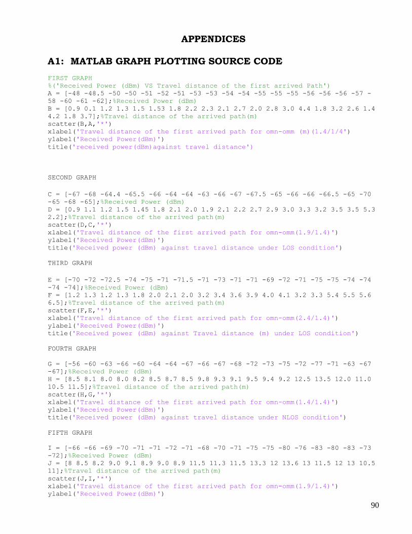
90

APPENDICES A1: MATLAB GRAPH PLOTTING SOURCE CODE

FIRST GRAPH

%('Received Power (dBm) VS Travel distance of the first arrived Path') A = [-48 -48.5 -50 -50 -51 -52 -51 -53 -53 -54 -54 -55 -55 -55 -56 -56 -56 -57 -

58 -60 -61 -62];%Received Power (dBm) B = [0.9 0.1 1.2 1.3 1.5 1.53 1.8 2.2 2.3 2.1 2.7 2.0 2.8 3.0 4.4 1.8 3.2 2.6 1.4

4.2 1.8 3.7];%Travel distance of the arrived path(m) scatter(B,A,'*') xlabel('Travel distance of the first arrived path for omn-omm (m)(1.4/1/4') ylabel('Received Power(dBm)') title('received power(dBm)against travel distance')

SECOND GRAPH

C = [-67 -68 -64.4 -65.5 -66 -64 -64 -63 -66 -67 -67.5 -65 -66 -66 -66.5 -65 -70

-65 -68 -65];%Received Power (dBm) D = [0.9 1.1 1.2 1.5 1.45 1.8 2.1 2.0 1.9 2.1 2.2 2.7 2.9 3.0 3.3 3.2 3.5 3.5 5.3

2.2];%Travel distance of the arrived path(m) scatter(D,C,'*') xlabel('Travel distance of the first arrived path for omn-omm(1.9/1.4)') ylabel('Received Power(dBm)') title('Received power (dBm) against travel distance under LOS condition')

THIRD GRAPH

E = [-70 -72 -72.5 -74 -75 -71 -71.5 -71 -73 -71 -71 -69 -72 -71 -75 -75 -74 -74

-74 -74];%Received Power (dBm) F = [1.2 1.3 1.2 1.3 1.8 2.0 2.1 2.0 3.2 3.4 3.6 3.9 4.0 4.1 3.2 3.3 5.4 5.5 5.6

6.5];%Travel distance of the arrived path(m) scatter(F,E,'*') xlabel('Travel distance of the first arrived path for omn-omm(2.4/1.4)') ylabel('Received Power(dBm)') title('Received power (dBm) against Travel distance (m) under LOS condition')

FOURTH GRAPH

G = [-56 -60 -63 -66 -60 -64 -64 -67 -66 -67 -68 -72 -73 -75 -72 -77 -71 -63 -67

-67];%Received Power (dBm) H = [8.5 8.1 8.0 8.0 8.2 8.5 8.7 8.5 9.8 9.3 9.1 9.5 9.4 9.2 12.5 13.5 12.0 11.0

10.5 11.5];%Travel distance of the arrived path(m) scatter(H,G,'*') xlabel('Travel distance of the first arrived path for omn-omm(1.4/1.4)') ylabel('Received Power(dBm)') title('Received power (dBm) against travel distance under NLOS condition')

FIFTH GRAPH

I = [-66 -66 -69 -70 -71 -71 -72 -71 -68 -70 -71 -75 -75 -80 -76 -83 -80 -83 -73

-72];%Received Power (dBm) J = [8 8.5 8.2 9.0 9.1 8.9 9.0 8.9 11.5 11.3 11.5 13.3 12 13.6 13 11.5 12 13 10.5

11];%Travel distance of the arrived path(m) scatter(J,I,'*') xlabel('Travel distance of the first arrived path for omn-omm(1.9/1.4)') ylabel('Received Power(dBm)')

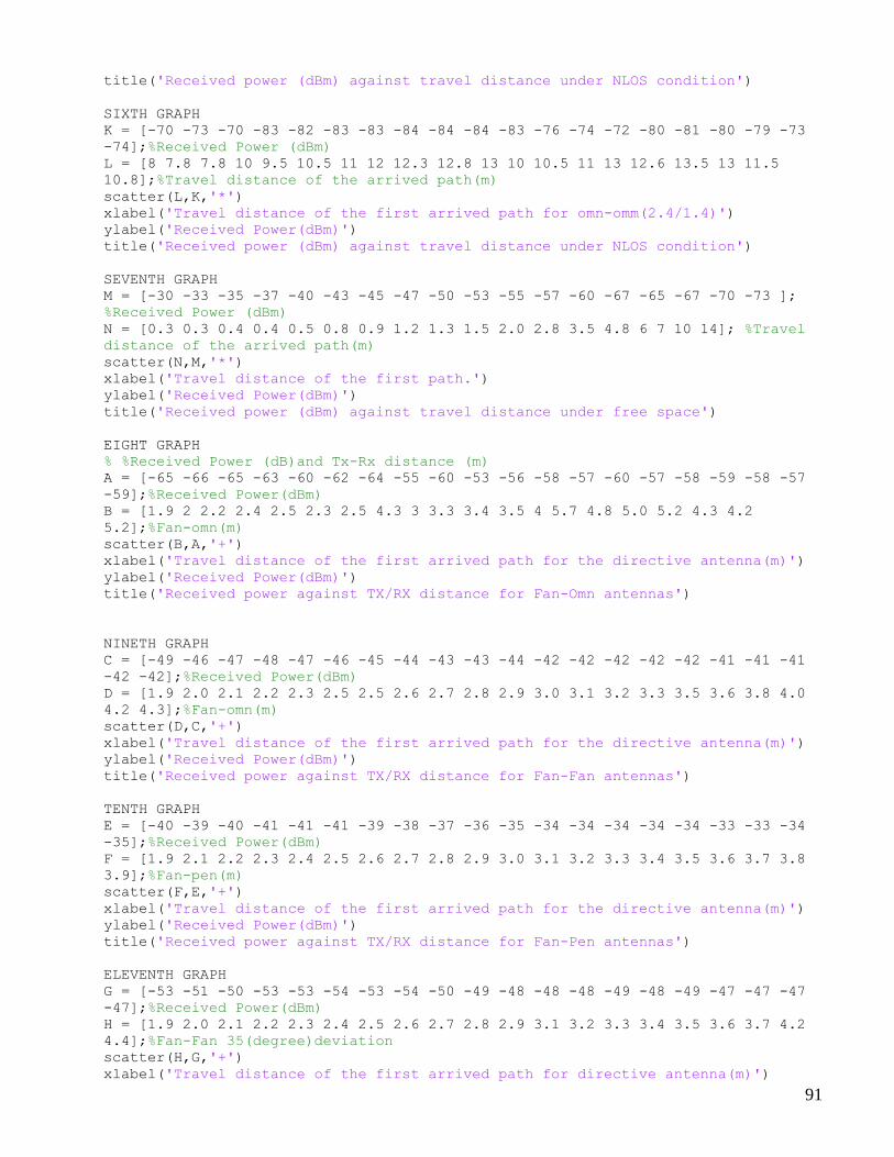
91

title('Received power (dBm) against travel distance under NLOS condition')

SIXTH GRAPH

K = [-70 -73 -70 -83 -82 -83 -83 -84 -84 -84 -83 -76 -74 -72 -80 -81 -80 -79 -73

-74];%Received Power (dBm) L = [8 7.8 7.8 10 9.5 10.5 11 12 12.3 12.8 13 10 10.5 11 13 12.6 13.5 13 11.5

10.8];%Travel distance of the arrived path(m) scatter(L,K,'*') xlabel('Travel distance of the first arrived path for omn-omm(2.4/1.4)') ylabel('Received Power(dBm)') title('Received power (dBm) against travel distance under NLOS condition')

SEVENTH GRAPH

M = [-30 -33 -35 -37 -40 -43 -45 -47 -50 -53 -55 -57 -60 -67 -65 -67 -70 -73 ];

%Received Power (dBm) N = [0.3 0.3 0.4 0.4 0.5 0.8 0.9 1.2 1.3 1.5 2.0 2.8 3.5 4.8 6 7 10 14]; %Travel

distance of the arrived path(m) scatter(N,M,'*') xlabel('Travel distance of the first path.') ylabel('Received Power(dBm)') title('Received power (dBm) against travel distance under free space')

EIGHT GRAPH

% %Received Power (dB)and Tx-Rx distance (m) A = [-65 -66 -65 -63 -60 -62 -64 -55 -60 -53 -56 -58 -57 -60 -57 -58 -59 -58 -57

-59];%Received Power(dBm) B = [1.9 2 2.2 2.4 2.5 2.3 2.5 4.3 3 3.3 3.4 3.5 4 5.7 4.8 5.0 5.2 4.3 4.2

5.2];%Fan-omn(m) scatter(B,A,'+') xlabel('Travel distance of the first arrived path for the directive antenna(m)') ylabel('Received Power(dBm)') title('Received power against TX/RX distance for Fan-Omn antennas')

NINETH GRAPH

C = [-49 -46 -47 -48 -47 -46 -45 -44 -43 -43 -44 -42 -42 -42 -42 -42 -41 -41 -41

-42 -42];%Received Power(dBm) D = [1.9 2.0 2.1 2.2 2.3 2.5 2.5 2.6 2.7 2.8 2.9 3.0 3.1 3.2 3.3 3.5 3.6 3.8 4.0

4.2 4.3];%Fan-omn(m) scatter(D,C,'+') xlabel('Travel distance of the first arrived path for the directive antenna(m)') ylabel('Received Power(dBm)') title('Received power against TX/RX distance for Fan-Fan antennas')

TENTH GRAPH

E = [-40 -39 -40 -41 -41 -41 -39 -38 -37 -36 -35 -34 -34 -34 -34 -34 -33 -33 -34

-35];%Received Power(dBm) F = [1.9 2.1 2.2 2.3 2.4 2.5 2.6 2.7 2.8 2.9 3.0 3.1 3.2 3.3 3.4 3.5 3.6 3.7 3.8

3.9];%Fan-pen(m) scatter(F,E,'+') xlabel('Travel distance of the first arrived path for the directive antenna(m)') ylabel('Received Power(dBm)') title('Received power against TX/RX distance for Fan-Pen antennas')

ELEVENTH GRAPH

G = [-53 -51 -50 -53 -53 -54 -53 -54 -50 -49 -48 -48 -48 -49 -48 -49 -47 -47 -47

-47];%Received Power(dBm) H = [1.9 2.0 2.1 2.2 2.3 2.4 2.5 2.6 2.7 2.8 2.9 3.1 3.2 3.3 3.4 3.5 3.6 3.7 4.2

4.4];%Fan-Fan 35(degree)deviation scatter(H,G,'+') xlabel('Travel distance of the first arrived path for directive antenna(m)')

92

ylabel('Received Power(dBm)') title('Received power against TX/RX distance for Fan-Fan 35(degree) deviation')

TWELVETH GRAPH I = [-66 -67 -67 -68 -65 -64 -64 -65 -65 -65 -65 -66 -66 -67 -65 -66 -66 -65 -66

-65];%Received Power(dBm) J = [1.9 2.0 2.1 2.2 2.3 2.4 2.5 2.6 2.7 2.9 3.0 3.2 3.3 3.5 3.6 3.7 4.2 4.3 4.4

4.5];%Fan-Pen 35(degree)deviation scatter(J,I,'+') xlabel('Travel distance of the first arrived path for directive antenna(m)') ylabel('Received Power(dBm)') title('Received power against TX/RX distance for Fan-Pen 35(degree) deviation')

THIRTEENTH GRAPH

%Plot K-factor against travel distance of the first arrived Path %dat gotten from experiment performed K1 = [2.1 1.2 1.8 0.4 1.0 1.1 1.2 1.4 1.6 1.8 0.9 1.0 1.0 1.2 1.3 1.4 1.6 1.5 1.8

1.3];%K-factor Los = [0.8 1 1 2 2.3 2.4 3 4.2 4.1 4.3 4.2 4.2 4.5 4.2 3.3 3.4 3.2 1.0 3.4

5.0];%Los omn-omn (1.4/1.4) scatter(Los,K1,'*') ylabel('K-factor') xlabel('Travel distance of the first arrived path for omnidirectional

antenna(m)(1.4/1.4)') title('K-factor against travel distance under LOS condition')

FOURTEENTH GRAPH

K2 = [0.3 0.2 0.4 0.6 1.8 1.7 0.4 0.5 0.5 0.7 0.5 0.3 0.5 0.1 1 1.1 1.0 0.7 0.9

0.6];%K-factor Los2 = [0.9 1.0 0.8 1.3 1.2 1.8 2.1 2.0 2.1 3.0 3.3 3.4 4.2 4.5 4.3 4.2 4.3 4.2

5.0 5.2];%Los omn-omn (1.9/1.4) scatter(Los2,K2,'*') ylabel('K-factor') xlabel('Travel distance of the first arrived path for omnidirectional

antenna(m)(1.9/1.4)') title('K-factor against travel distance under LOS condition')

FIFTEENTH GRAPH

K3 =[0.1 0.3 0.5 0.2 0.1 0.4 0.5 0.3 0.1 0.2 0.4 1.0 0.9 0.7 1.0 0.8 0.4 0.1 0.2

0.5];%K-factor Los3 = [1.2 1.3 1.0 1.8 1.9 2.1 2.2 2.3 2.5 2.1 2.2 2.4 2.3 2.5 3.4 3.3 3.2 4.3

5.2 5.3];%Los omn-omn (2.4/1.4) scatter(Los3,K3,'*') ylabel('K-factor') xlabel('Travel distance of the first arrived path for omn-omn(m)(2.4/1.4)') title('K-factor against travel distance under LOS condition')

SIXTEENTH GRAPH

%data values for NLos omn-omn gotten from experiment K4 = [4.8 2.0 2.1 1.9 1.5 1.8 1.7 1.9 1.5 1.8 0.1 0.4 0.3 0.2 0.5 0.4 0.3 0.2 0.3

1.8];%K-factor Los4 = [8 7.8 8.4 8.2 8.1 8.5 8.6 9.2 9.3 9.0 10.4 10.3 11.2 12.3 11.4 11.4 11.6

12.4 13.3 13.5];%NLos omn-omn (1.4/1.4) scatter(Los4,K4,'*') ylabel('K-factor') xlabel('Travel distance of the first arrived path for omn-omn

antennas(m)(1.4/1.4)') title('k-factor against travel distance under NLOS condition')

SEVENTEENTH GRAPH

93

K5 = [7.4 7.2 8.9 4.9 2.1 2.3 1.8 1.9 2.0 1.5 1.3 2.1 2.0 2.3 2.4 2.6 2.8 1.0 1.1

1.3];%K-factor Los5 = [8.9 8.1 8.7 9.1 9.3 9.4 10.4 11.0 10.8 10.7 11.4 12.4 12.5 13.0 9.4 9.6

12.4 13.0 13.3 13.3];%NLos omn-omn (1.9/1.4) scatter(Los3,K3,'*') ylabel('K-factor') xlabel('Travel distance of the first arrived path for omn-omn

antennas(m)(1.9/1.4)') title('K-factor against travel distance under NLOS condition')

EIGHTEENTH GRAPH

K6 = [5.3 0.5 1.2 0.3 0.4 0.3 0.2 0.3 0.4 0.3 0.5 1.2 1.3 1.5 0.3 0.6 1.3 2.1

2.3 3.5];%K-factor Los6 = [8.3 8.6 9.1 9.3 8.4 10.3 10.6 11.0 10.4 8.4 8.6 10.4 13.0 13.3 12.1 12.3

8.6 8.4 9.3 9.4];%NLos omn-omn (2.4/1.4) scatter(Los6,K6,'*') ylabel('K-factor') xlabel('Travel distance of the first arrived path for omn-omn

antennas(m)(2.4/1.4)') title('K-factor against travel distance under NLOS condition')

NINETEENTH GRAPH

%plot of K-factor against Tx-Rx distance(m) K1 = [0.8 1.0 1.0 1.2 1.5 1.4 1.6 1.8 2.1 2.3 1.3 1.5 5.0 4.3 4.8 3.0 3.5 3.6 4.0

2.0];%K-factor F1 = [1.9 2.0 2.2 2.3 2.5 3.0 2.8 3.4 3.6 3.7 3.5 3.6 4.0 4.2 4.3 4.2 4.6 5.0 5.4

5.3];%Fan-omn scatter(F1,K1,'*') xlabel('Travel distance of the first arrived path for Fan-omn antennas(m)') ylabel('K-factor') title('K-factor against TX/RX distance')

TWENTIETH GRAPH

K2 = [10.0 11.0 10 13 12 14 15 14 16 12 11 10 9 8 7 10 12 13 11 13];%K-factor F2 = [1.9 2 2.3 2.3 3.4 3.0 3.1 3.2 3.4 4 4.2 4.4 4.3 5.0 5.3 5.4 5.6 4.3 4.2

4.1];%Fan-omn scatter(F2,K2,'*') xlabel('Travel distance of the first arrived path for Fan-Fan antennas(m)') ylabel('K-factor') title('K-factor against TX/RX distance')

TWENTY-FIRST GRAPH

K3 = [11 12 15 18 16 20 21 23 36 20 21 18 19 24 16 12 11 10 13 14];%K-factor F3 = [1.9 2 2.2 2.4 3.4 3.2 3.3 4.6 4.2 4.8 3.4 5.3 5.2 4.8 4.6 3.6 4.8 5 5.3 5.2

];%Fan-omn scatter(F3,K3,'*') xlabel('Travel distance of the first arrived path for Fan-Pen antennas(m)') ylabel('K-factor') title('K-factor against TX/RX distance')

TWENTY-SECOND GRAPH

%this the datas for the anagular deviation of 35degree K4 = [8 10 9 8 10 7 8 10 6 7 8 10 11 12 11 6 7 8 10 20 ];%K-factor F4 = [1.9 2 2.2 2.3 2.4 4 4.2 3.6 4.1 4.3 3.6 3.2 3.3 3.4 4.2 4.3 5 5.6 5.7

5.2];%Fan-fan 35degree deviation scatter(F4,K4,'*') xlabel('Travel distance of the first arrived path for Fan-Fan antennas(m)') ylabel('K-factor') title(' K-factor against TX/RX distance with 35(degrees) deviation')

94

TWENTY-THIRD GRAPH K5 = [4 1 2 4 5 6 1 3 4 5 7 2 4 6 3 2 5 4 3 4 ];%K-factor F5 = [1.9 2.0 2.3 2.4 2 3 3.4 4.6 4.1 4.3 5 5.2 5.3 4.3 4.4 4.6 4.1 4.3 4.2

5];%Fan-pen 35degree deviation scatter(F3,K3,'*') xlabel('Travel distance of the first arrived path for Fan-Pen antennas(m)') ylabel('K-factor') title('K-factor against TX/RX distance with 35(degrees) diviation')

TWENTY-FOURTH GRAPH

%Plot Rms delay spread against ttavel distance of the first arrived Path R1 = [5 4 4 6 8 9 4 5 6 5 4 7 8 10 6 5 10 4 5 6 ];%RDS(ns) Los1 = [0.8 0.9 1 2.2 2.3 2.2 3 1.6 3.4 4 4.1 5.6 5.4 5 5.2 3.2 3.4 2.4 2.3

3.1];%Los (omn-omn(1.4/1.4) scatter(Los1,R1,'*') xlabel('Travel distance of the first arrived path for omn-omn

antennas(m)(1.4/1.4))') ylabel('RMS delay spread(ns)') title('RMS delay spread against travel distance under LOS condition')

TWENTY-FIFTH GRAPH

R2 = [11 10 12 15 16 14 14 14 13 12 13 14 11 12 10 9 8 10 11 13];%RDS(ns) Los2 = [0.7 0.9 1 1.1 1.4 2.3 2.4 2.6 3 3.2 2.4 3 3.1 3.6 3.2 4.3 4.4 3.1 4.1

5.6];%%Los (omn-omn(1.9/1.4)) scatter(Los2,R2,'*') xlabel('Travel distance of the first arrived path for omn-omn

antennas(m)(1.9/1.4))') ylabel('RMS delay spread(ns)') title('RMS delay spread against travel distance under LOS condition')

TWENTY-SIXTH GRAPH R3 = [16 18 20 22 24 18 19 17 24 16 18 19 20 21 24 23 25 26 28 16];%RDS(ns) Los3 = [1.2 1.3 2.4 2.6 2.3 2.5 3.4 3.8 4.6 4.2 4.1 4.3 4.4 5 5.2 2.3 4.3 3.4 4.1

5];%Los (omn-omn(2.4/1.4)) scatter(Los3,R3,'*') xlabel(' Travel distance of the first arrived path for omn-omn

antennas(m)(2.4/1.4))') ylabel('RMS delay spread(ns)') title('RMS delay spread against travel distance under LOS condition')

TWENTY-SEVENTH GRAPH

R4 = [4 6 5 7 8 10 12 15 12 13 14 13 14 14 13 10 9 8 8 6];%RDS(ns) Los4 = [8 8.1 7.9 9.4 10.1 10.3 11.4 12.0 9.6 9.8 10.0 10.5 11.2 12.0 10.0 11.3

9.3 13.4 13.2 11.3];%NLos (omn-omn(1.4/1.4)) scatter(Los4,R4,'*') xlabel('Travel distance of the first arrived path for omn-omn

antennas(m)(1.4/1.4))') ylabel('RMS delay spread(ns)') title('RMS delay spread against travel distance under NLOS condition')

TWENTY-EIGHT GRAPH

R5 = [8 9 10 13 20 15 16 18 17 16 15 14 25 22 23 25 18 19 20 14]; Los5 = [8.3 8.5 8.1 10.4 11.2 10.4 10.5 11.3 12 12.4 9.3 9.5 10.3 11.4 10 9.3 9.6

9.8 13.4 13.8]; scatter(Los5,R5,'*') xlabel('Travel distance of the first arrived path for omn-omn

antennas(m)(1.9/1.4))') ylabel('RMS delay spread(ns)') title('RMS delay spread against travel distance under NLOS condition')

95

TWENTY-NINETH GRAPH R6 = [9 11 13 12 15 16 20 24 30 33 34 31 20 21 18 17 14 15 13 20]; Los6 = [8 10 8.3 8.2 10.4 11.3 12.4 13.3 11.6 11.8 8.4 13.4 10.3 10.2 9.3 10.3

10.4 11.3 13.3 12.4]; scatter(Los6,R6,'*') xlabel('Travel distance of the first arrived for omn-omn antennas(m)(2.4/1.4))') ylabel('RMS delay spread(ns)') title('RMS delay spread against travel distance under NLOS condition')

THIRTIETTH GRAPH

%RSM delay spread (ns) against Tx-Rx distance(m) A = [37 38 36 32 30 31 26 24 25 10 9 6 5 6 8 7 11 10 12 22]; B = [1.9 2 2.4 2.3 2.5 2.6 2.8 2.9 3.1 3.3 3.4 3.5 3.5 3.6 4.2 4.3 4.5 4.6 5.3

5.2]; scatter(B,A,'*') xlabel('Travel distance of the first arrived path for Fan-Omn antennas(m)') ylabel('RMS delay spread(ns)') title('RMS delay spread against TX/RX distance')

THIRTY-FIRST GRAPH

R2 = [1 1.2 1 1.2 2.2 3 1.2 2 1.3 2 1.2 1 1.3 1 1 2 1 2.2 1.2 2 ]; F2 = [1.9 2 2.1 2.3 2.4 3.1 3.6 3.5 3.4 3.2 4.3 4.5 4.4 4.6 5.1 5.3 5.2 5.3 3.2

5.4]; scatter(F2,R2,'*') xlabel('Travel distance of the first arrived path for Fan-Fan antennas(m)') ylabel('RMS delay spread(ns)') title('RMS delay spread against TX/RX distance')

THIRTY-SECOND GRAPH

R3 = [1.1 1.2 1.15 1.15 1.2 1.1 1.1 1.2 1.15 1.1 1.15 1.1 0.8 0.9 0.8 1.0 1.1 1.0

0.9 0.8]; F3 = [1.9 2 2.2 2.3 2.2 3.4 3.6 4.2 3.5 3.6 4.2 3.5 3.6 4.3 4.4 4.3 4.2 4.1 5.2

5.3 ]; scatter(F3,R3,'*') xlabel('Travel distance of the first arrived path for Fan-Pen antennas(m)') ylabel('RMS delay spread(ns)') title('RMS delay spread against TX/RX distance')

THIRTY-THIRD GRAPH R4 = [1.8 1.4 1.5 1.4 1.3 1.2 1.45 1.43 1.42 1.46 1.8 1.9 2.2 2 2.35 2.1 1.6 1.8

1.4 1.45]; F4 = [1.9 2.0 2.2 2 1.9 2.4 2.3 4.6 4.3 3.4 3.2 3.3 3.2 3.4 5.6 5.4 5.2 4.6 4.3

4.6]; scatter(F4,R4,'*') xlabel('Travel distance of the first arrived for Fan-Fan antennas(m)') ylabel('RMS delay spread(ns)') title('RMS delay spread against TX/RX distance with 35(degrees) diviation')

THIRTY-FOURTH GRAPH

R5 = [3.2 3.9 3.5 2.8 3.3 3.0 3.2 2.9 2.8 2.5 1.5 1.1 1.4 1.5 1.7 1.8 2.2 2.4 1.8

2.0]; F5 = [1.9 2 2.4 2.6 3 3.2 3.1 4 4.3 5.2 5.6 5.3 5.2 3.4 3.6 3.4 2.4 2.6 5.4 3.4]; scatter(F5,R5,'*') xlabel('Travel distance of the first arrived path for Fan-Pen antennas(m)') ylabel('RMS delay spread(ns)') title('RMS delay spread against TX/RX distance with 35(degrees) deviation')

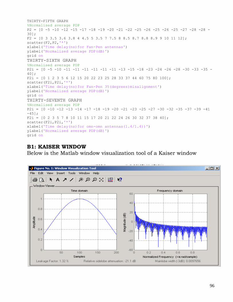
96

THIRTY-FIFTH GRAPH

%Normalised average PDP P2 = [0 -5 -10 -12 -15 -17 -18 -19 -20 -21 -22 -25 -26 -25 -26 -25 -27 -28 -28 -

30]; F2 = [0 3 3.5 3.6 3.8 4 4.5 5 3.5 7 7.5 8 8.5 8.7 8.8 8.9 9 10 11 12]; scatter(F2,P2,'*') xlabel('Time delay(ns)for Fan-Pen antennas') ylabel('Normalized average PDP(dB)') grid on

THIRTY-SIXTH GRAPH %Normalised average PDP P2i = [0 -5 -10 -11 -11 -11 -11 -11 -11 -13 -15 -18 -23 -24 -26 -28 -30 -33 -35 -

40]; F2i = [0 1 2 3 5 6 12 15 20 22 23 25 28 33 37 44 60 75 80 100]; scatter(F2i,P2i,'*') xlabel('Time delay(ns)for Fan-Pen 35(degrees)misalignment') ylabel('Normalized average PDP(dB)') grid on

THIRTY-SEVENTH GRAPH %Normalised average PDP P2i = [0 -10 -12 -13 -14 -17 -18 -19 -20 -21 -23 -25 -27 -30 -32 -35 -37 -39 -41

-45]; F2i = [0 2 3 5 7 8 10 11 15 17 20 21 22 24 26 30 32 37 38 40]; scatter(F2i,P2i,'*') xlabel('Time delay(ns)for omn-omn antennas(1.4/1.4))') ylabel('Normalized average PDP(dB)') grid on

B1: KAISER WINDOW

Below is the Matlab window visualization tool of a Kaiser window