mimo channel correlation analysis part 1: mimo …richiej/seminar/mu__mimo_3_28_2014_v0.0.pdflsr 1...
TRANSCRIPT

LSR 1
MIMO Channel Correlation AnalysisPart 1: MIMO Channel Realizations
March 28,2014

LSR 2LSRMIMO
• Speaker Introduction
• BSEET, MSOE, 1985.
• MSEE, Marquette University, 1987
• Chief Technology Officer, LS Research, LLC
• Adjunct Assistant Professor, MSOE
• Rockwell-Collins, Harris Government Communication Systems.• Agenda
•MIMO (Spatial Multiplexing).
• Channel Estimation
• Channel Capacity
• Antenna Pattern Interactions with Channel Matrix

LSR 3LSRMIMO
• Multipath Channel

LSR 4LSRMIMO
• Multipath Channel – Null Density and Antenna Diversity
2

LSR 5LSRMIMO
• Multiple Input, Multiple Output MIMO (Spatial Multiplexing).
2221212
2121111
shshrshshr
SHRss
hhhh
rr
2
1
2221
1211
2
1
TX1 RX1
RX2TX2
s1,s2,s3,s4,s5,... s1,s2,s3,s4,s5,...
h11
h22
21
s2,s4,s6...
s1,s3,s5,... r1,r3,r5,...
r2,r4,r6,...

LSR 6LSRMIMO
• Symbol Recovery
Rhhhh
hhhh
RH
HadjRHS
T
21122211
1112
2122
1
211121
212122
2
1
1121
1222
2112221121122211
1121
1222
1 1rhrh
rhrhB
rr
hhhh
hhhhR
hhhhhhhh
RH
HadjRHS
• Symbol Recovery

LSR 7LSRMIMO
• Special Case: One Channel Completely Faded: h11 = 0
12
1
21
2
2112
122
121
212122
21122
1
2
1
21
1222
21122112
21
1222
1
01
001
00
hr
hr
hhrh
rhrhrh
hhss
rr
hhh
hhR
hhh
hh
RH
HadjRHS
• Special Case: When all coefficients are the same: |H| is zero, matrix is singular.

LSR 8LSRMIMO
• Goal is change many scattered communication channels into a few dominant channels:
• Goal is to track and utilize available ‘eigenbeams’
• First step is to examine process with known channel state information (deterministic)
• Next step is perform eigenbeam tracking based on channel statistics (covariance matrix, Kalman Filter), and also incorporate interference suppression.

LSR 9LSRMIMO
• Additional Insight into Channel Matrix: Singular Value Decomposition: SVD.
xAx
• Eigenvalues, Eigenvectors
0det
0det
0)det()det(
0
0;00
11
IAxIAIA
IAIAadjxIA
IAIAadj
IAxIAIAx
xxIAxAx
• Characteristic Equation, roots are eigenvalues
n
IAIA
....,,0)det(
321
LSR 10LSRMIMO
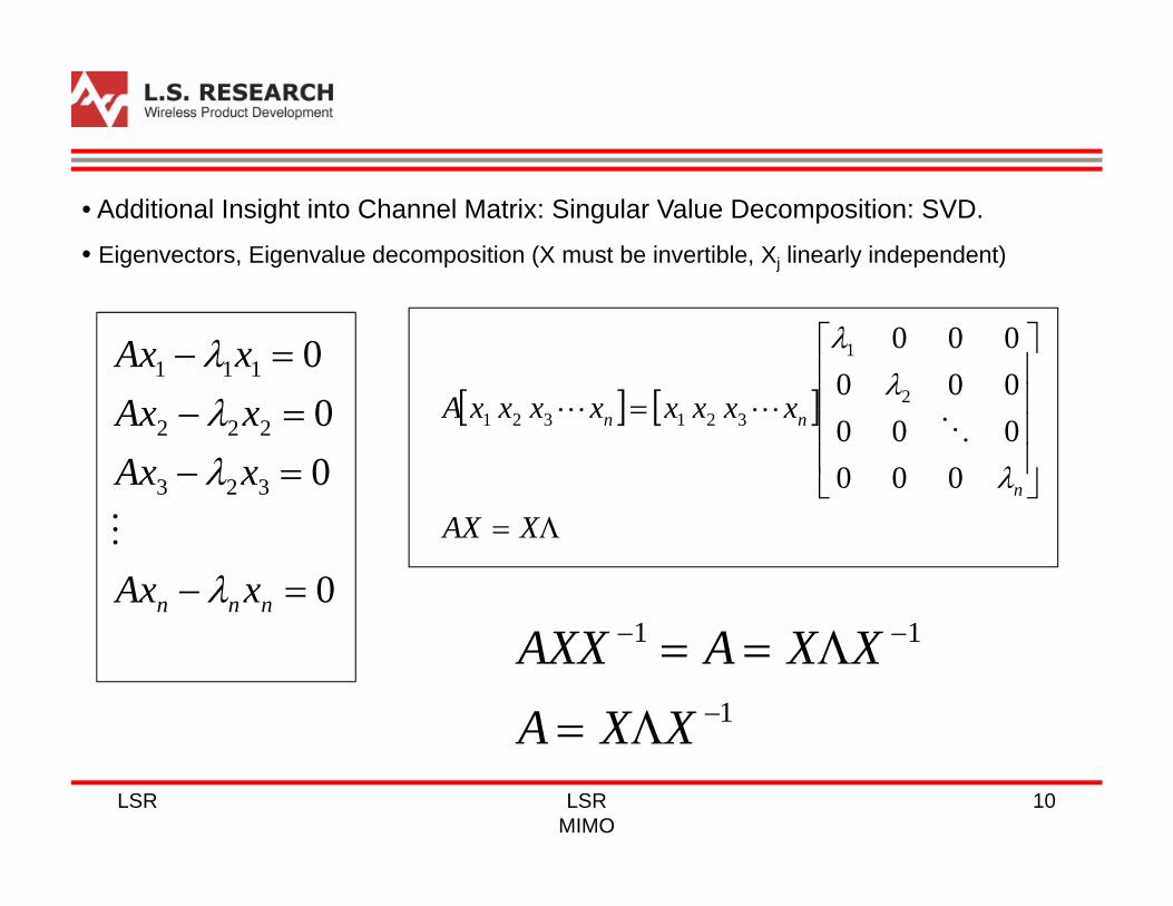
• Additional Insight into Channel Matrix: Singular Value Decomposition: SVD.
• Eigenvectors, Eigenvalue decomposition (X must be invertible, Xj linearly independent)
0
00
0
323
222
111
nnn xAx
xAxxAxxAx
XAX
xxxxxxxxA
n
nn
000000000000
2
1
321321
1
11
XXAXXAAXX

LSR 11LSRMIMO
• Additional Insight into Channel Matrix: Singular Value Decomposition: SVD.
• Singular Value (non negative scalar), Singular vector pair, u,v:
vuAuAv
H
HH VUAUAV
n
nn uuuuvvvvA
000000000000
2
1
321321

LSR 12LSRMIMO
• Additional Insight into Channel Matrix: Singular Value Decomposition: SVD.
• Solve for A and AH: 1 VUA
11 UVUUAA HHHHH VUAUAV
• Eigenvalue decomposition of A AH to find and U:
UUAAUUAA
UUUVVUAVUAA
H
H
HH
I
H
A
H
1
1111
• U is a unitary (complex) or orthogonal (real) matrix.
LSR 13LSRMIMO
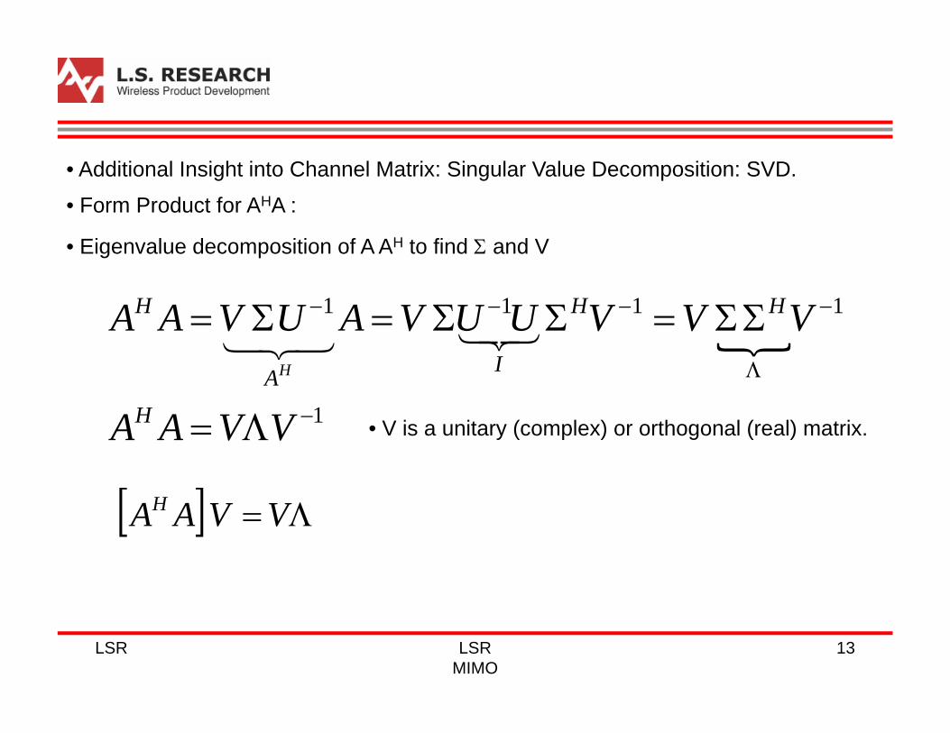
• Additional Insight into Channel Matrix: Singular Value Decomposition: SVD.
• Form Product for AHA :
1
1111
VVAA
VVVUUVAUVAA
H
HH
IA
H
H
• Eigenvalue decomposition of A AH to find and V
VVAAH
• V is a unitary (complex) or orthogonal (real) matrix.

LSR 14LSRMIMO
• Additional Insight into Channel Matrix: Singular Value Decomposition: SVD.
• Form SVD 1 VUA
1321
2
1
321
000000000000
n
n
n vvvvuuuuA
2
22
21
*
*2
*1
2
1
000000000000
000000000000
000000000000
nnn
H
n
000000000000
2
1
21

LSR 15LSRMIMO
• Additional Insight into Channel Matrix: Singular Value Decomposition: SVD.
• Form SVD of Channel Matrix
1 ΣVUH• U and V are unitary (complex)
H
H
VVUU
1
1
HΣVUH

LSR 16LSRMIMO
• Additional Insight into Channel Matrix: Singular Value Decomposition: SVD.
• Form SVD of Channel Matrix
HΣVUH
wxHy • Input / Output Relation:
noIN,, 00~ CNCN Kw
xUwxUyxVx
H
H
H
~~
• Define Pre- and Post-Processing Steps (Beamforming):

LSR 17LSRMIMO
• Additional Insight into Channel Matrix: Singular Value Decomposition: SVD.
• Form SVD of Channel Matrix
wxΣywUxVΣVUUyUU
wxVΣVUyU
~~~~~
~~
HHHH
H
noIN,, 00~~ CNCN Kw
• Since UH is orthogonal matrix, covariance matrix, K=UHU=I is unchanged.

LSR 18LSRMIMO
• Additional Insight into Channel Matrix: Singular Value Decomposition: SVD.
• With proper pre- and post-processing, the channel exists as n parallel channels:
wxΣy ~~~
nnnn w
ww
x
xx
y
yy
~
~~
~
~~
000000000000
~
~~
1
1
2
1
2
1
1
1

LSR 19LSRMIMO
• Additional Insight into Channel Matrix: Singular Value Decomposition: SVD.
• With proper pre- and post-processing, the channel exists as n parallel channels:
VHx~
1
2
n
U
+
V x
1~w
+
2~w
+
nw~
y~UHy
CHANNELPRE-PROCESSING POST-PROCESSING

LSR 20LSRMIMO
• Additional Insight into Channel Matrix: Singular Value Decomposition: SVD.
• With proper pre- and post-processing, the channel exists as n parallel channels:
• n are the individual gains of each parallel channel or eigenbeams.
• V is a transmit beamforming matrix (pre-coding).
• UH is a receive beamforming matrix (post-coding).
• The beamforming matrices ‘equalize’ the channel into dominant, parallel eigenbeams:
• Each eigenbeam has an associated gain (i’s in diagonal matrix).
• Since each eigenbeam has different gain, distribute power to emphasize channels with high gain and deemphasize channels with low gain.
• Power allocation can be optimized by the Waterfilling principle.

LSR 21LSRMIMO
• MIMO Ergodic Channel Capacity.
• Assumptions: Equal Power distribution (no transmit channel knowledge, water-filling or other power distribution optimization algorithms [1]:
Hz
bits
NEC H
xo
nr
sec1detlog2 HHKI
• E = expected value, det = determinant, AH=Hermitian Transpose, Kx = transmit covariance matrix ratio, nr = number of transmitters, nt = number of transmitters, H = channel matrix.
[1] Fundamentals of Wireless Communication, D. Tse and P. Viswanath, Cambridge University Press, 2005..
tnt
tx n
P IK
• For equal power applied at each channel, covariance, Kx becomes:

LSR 22LSRMIMO
• MIMO Ergodic Channel Capacity.
• Assume that pre- and post-coding is forming eigenbeams such that
Hz
bits
nP
NEC H
nto
n tr
sec1detlog2 ΣIΣI
ΣH
Hz
bits
NnPEC H
not
n tr
secdetlog2 ΣΣII
Hz
bits
NnPEC H
otnr
secdetlog2 ΣΣI

LSR 23LSRMIMO
• MIMO Ergodic Channel Capacity.
Hz
bits
nP
NEC H
nto
n tr
sec1detlog2 ΣIΣI
Hz
bits
NnPEC H
not
n tr
secdetlog2 ΣΣII
Hz
bits
NnPEC H
otnr
secdetlog2 ΣΣI

LSR 24LSRMIMO
• MIMO Ergodic Channel Capacity.
Hz
bits
NnPEC H
otnr
secdetlog2 ΣΣI
ii
n
iaA
1)det(
Hz
bits
NnP
ECot
in
i
r sec1log2
12
Hz
bits
NnP
ECrn
i ot
i sec1log1
2
2

LSR 25LSRMIMO
• MIMO Ergodic Channel Capacity with Equal Power Allocation, Rayleigh Fading.
-20 -15 -10 -5 0 5 10 15 200
2
4
6
8
10
12
14
16
SNR in dB
Cap
acity
bits
/s/H
z
Channel Capacity for Various MIMO Channel Multiplexing Schemes
nt = 1 , nr = 1nt = 2 , nr = 2nt = 3 , nr = 3nt = 4 , nr = 4nt = 5 , nr = 5

LSR 26LSRMIMO
• pdf of singular value gains, Rayleigh Fading.
0 0.5 1 1.5 2 2.5 3 3.5 40
0.01
0.02
0.03
0.04
0.05
0.06pd
f of e
lem
ents
in m
atrix
land
a in
svd
dec
ompo
sitio
n of
mar
ix H
nt = 1 , nr = 1nt = 2 , nr = 2nt = 3 , nr = 3nt = 4 , nr = 4nt = 5 , nr = 5

LSR 27LSRMIMO
• MIMO Ergodic Channel Capacity with Waterfilling Power Allocation, Rayleigh Fading.
-20 -15 -10 -5 0 5 10 15 200
2
4
6
8
10
12
14
16
18
SNR in dB
Cap
acity
bits
/s/H
zChannel Capacity for Various MIMO Channel Multiplexing Schemes
nt = 1 , nr = 1nt = 2 , nr = 2nt = 3 , nr = 3nt = 4 , nr = 4nt = 5 , nr = 5

LSR 28LSRMIMO
• Waterfilling Power Allocation
1 2 3 4 5 6 7 80
10
20
30
40
50
60
70
80
90
100
Channel
No/
2Waterfilling Power Allocation

LSR 29LSRMIMO
• Waterfilling Power Allocation – Optimal allocation of power across eigenbeams.
• Use method of Lagrange Multipliers
• Calculate the Langrangian: = function to be maximized over the constraint function:
),( yxfcyxg ),(
cyxgyxfyx ,,),,(
0),,(
0),,(
0),,(0),,(,,
yxyyx
xyx
yxyx

LSR 30LSRMIMO
• Waterfilling Power Allocation – Optimal allocation of power across eigenbeam channels.
• Maximize Channel Capacity [bits/sec/Hz]:
c
cNnc
N
n o
nn
PPPPN NP
C1
2
2,...,,1logmax
21
• Subject to the constraint (P=power per channel):
0;1
ntc
N
nn PPPNP
c
• The Lagrangian (C maximized in nats rather than bits):
PNPN
PPPP c
N
nn
N
n o
nnNno
cc
c11
2
1log,,...,...,

LSR 31LSRMIMO
•Kuhn-Tucker Condition for Optimality:
0000
n
n
n PP
P
01log11
2
PNPN
PPP c
N
nn
N
n o
nn
nn
cc
0
12
2
o
nn
o
n
n
NPN
P

LSR 32LSRMIMO
•Kuhn-Tucker Condition for Optimality:
01
2
nn
on PNP
nn
o PN2
1
21
n
on
NP
0,1max 2
n
on
NP

LSR 33LSRMIMO
•Kuhn-Tucker Condition for Optimality:
011
t
N
nnc
N
nn PPPNP
cc
011
t
N
nnc
N
nn PPPNP
cc
cN
nn
c
PN
P1
1
cN
n n
o
c
NN
P1
2 0,1max1
cN
nnt PP
1

LSR 34LSRMIMO
• Algorithm: Initial Power Allocation:
2
1
n
o
in
NPi
ccc N
n n
ot
N
n cn
o
cc
tN
n n
o
ci
NPN
NNN
PNN
P1
21
21
21111
cccc N
n n
o
ci
N
n n
o
c
N
n ic
N
n n
o
ic
NN
NNN
NN
P1
21
211
21111111
21
21
n
oN
n n
ot
cn
NNPN
Pc
i

LSR 35LSRMIMO
• Algorithm: Determine Non-Negative Powers:
0,1max0,max 21
2n
oN
n n
ot
cn
NNPN
Pc
i
• Algorithm: Retain only channels with Na <=Np positive power allocations:
2
12
1
np
oN
n np
ot
ppn
NNPN
Pp

LSR 36LSRMIMO
• Next Steps
• Examine Eigenvectors as Beamforming vectors.
• Examine Eigenvectors as Eigenspace basis (unit vectors, direction).
• Examine beam radiation patterns and power azimuth spectrum suggested by channel matrix and beamforming vectors.
• Present the notion of beam tracking in both deterministic beam forming and stochasitic beam forming.

LSR 37LSRMIMO
• Thanks
• Dr. Ishii and Dr. Ritchie.
• Audience: Students, Faculty, Community professionals.
•
• Q and A Forum