minimal-energy driving strategy for high-speed …acsp.ece.cornell.edu/papers/lietal13tits.pdf ·...

1642 IEEE TRANSACTIONS ON INTELLIGENT TRANSPORTATION SYSTEMS, VOL. 14, NO. 4, DECEMBER 2013

Minimal-Energy Driving Strategy for High-SpeedElectric Train With Hybrid System Model

Liang Li, Member, IEEE, Wei Dong, Member, IEEE, Yindong Ji, Member, IEEE,Zengke Zhang, and Lang Tong, Fellow, IEEE

Abstract—This paper studies a minimal-energy driving strategyfor high-speed electric trains with a fixed travel time. A hybridsystem model is proposed to describe the new characteristics ofhigh-speed electric trains, including the extended speed range,energy efficiency, and regenerative braking. Based on this model,train driving is characterized by the gear sequence and the switch-ing locations. An approximate gradient information is derived viathe variational principle. To avoid a combinatorial explosion, thegear sequence is fixed by a priori knowledge. Then, a gradient-based exterior point method is proposed to calculate the optimaldriving. In the case study, the minimal-energy driving with a fixedtravel time for CRH-3 is investigated, and the result reveals somenew understandings for high-speed electric train drive. Addition-ally, the tradeoff relationship between energy consumption andtravel time is quantitatively studied, which is helpful in assigningan appropriate travel time for high-speed trains.

Index Terms—Energy efficiency, high-speed electric tain, hybridsystem model, marginal power, minimal-energy driving.

I. INTRODUCTION

E LECTRIC trains, with their advantages of convenienceand environmental performance, have been attracting in-

creasing attention recently. Many countries in the world havebegun to develop or expand their own electric train projects.However, this campaign is seriously impeded by the vast en-ergy consumption of electric trains. Currently, there have beenmany techniques proposed to reduce the energy consumptionof electric trains [1], such as adopting motorcoach patterns tomake the train more compact and lighter, changing the outlookof locomotives to reduce the aerodynamic resistance, equippingthe regenerative brake to feed back the kinetic energy, etc. Onthe other hand, a proper driving strategy can also reduce theenergy consumption of electric trains. Many scholars and re-

Manuscript received March 11, 2012; revised August 12, 2012, January 8,2013, and April 27, 2013; accepted May 21, 2013. Date of publication June 20,2013; date of current version November 26, 2013. This work was supportedin part by the Natural Science Foundation of China under Grants 61104019and 61004070, by the National Key Technology Research and DevelopmentProgram under Grant 2009BAG12A08, and by the Tsinghua University Ini-tiative Scientific Research Program. The Associate Editor for this paper wasA. Eskandarian.

L. Li, W. Dong, Y. Ji, and Z. Zhang are with the Department of Automa-tion, Tsinghua University, and Tsinghua National Laboratory for InformationScience and Technology, Beijing 100084, China (e-mail: [email protected]; [email protected]; [email protected];[email protected]).

L. Tong is with the School of Electrical and Computer Engineering, CornellUniversity, Ithaca, NY 14853 USA (e-mail: [email protected]).

Color versions of one or more of the figures in this paper are available onlineat http://ieeexplore.ieee.org.

Digital Object Identifier 10.1109/TITS.2013.2265395

searchers have therefore been searching for the optimal drivingstrategy over the years.

The original research on optimal driving of electric trains wasbegun in the 1960s by Ichikawa [2], in which the optimizationtheory was primarily applied to train operation. The earlymathematical model of trains took continuous control variables,such as acceleration and tractive effort, which facilitates in-vestigation into optimal driving with the maximum principle(MP) [3]. In [4], train motion was formulated in the form ofkinetic energy, and a parameterized optimal control effort wasderived via the MP. The work in [5] took the relative tractiveand braking forces as control variables and obtained a similaroptimal control effort. The energy consumption of trains wasexpressed in the form of current and voltage in [6], and the MPwas used to optimize the relative traction effort. Train drivingcan be also optimized by dynamic programming (DP) (see [7]).The nonlinear and constrained optimization problem in trainoperation can be handled by heuristic DP [8]. When discretizingthe route line, discrete DP can be applied to optimize thetractive and brake efforts [9]. As the continuous control variableis not consistent with the actual train operation, these theoreticalfruits did not received deserved attention from the industrialcommunity.

Considering the operating mechanism of modern trains,Cheng and Howlett presented a model taking the discretethrottle as a control variable [10], in which each throttle cor-responds to a traction power or a fuel supply rate. Based on thisdiscrete model, the optimal driving strategy was respectivelyinvestigated on the level track with a speed limit [11] and on thenonzero slope track [12]. Furthermore, the necessary conditionsfor optimal control on the steep track were systematicallystudied in [13]. To simplify the throttle set, three throttles areusually considered in the given works, which correspond to themaximum traction, coasting, and maximum braking, respec-tively. It has been proven that any ideal strategy of continuousdriving control can be approximated as closely as possible bythese three throttles [11]. In fact, when considering the energyefficiency of throttles, this simplification may no longer besuitable. This will be illustrated later in this paper.

Based on previous works, the train driving between stationscan be generally divided into four stages, i.e., traction, cruis-ing, coasting, and braking. Therefore, the train driving can becharacterized by the switching locations of stages. This turnsout to be a nonlinear optimization problem. The metaheuristicmethods were used to handle this kind of problem, e.g., geneticalgorithm [14], tabu search, and ant colony optimization [15].The simulated annealing algorithm in [16] was applied to search

1524-9050 © 2013 IEEE

LI et al.: MINIMAL-ENERGY DRIVING STRATEGY FOR HIGH-SPEED ELECTRIC TRAIN 1643

the cruising speed and the switching locations. With the helpof improved computation capability, some simulation modelswere also presented to study the train’s optimal driving [17]. Atime-driven train performance simulation model was proposedin [18]. Based on this model, the energy consumption and triptime were studied with regard to the coasting position. Thework in [19] developed an automatic-train-operation simulationmodel, which integrates a predictive fuzzy controller to regulatethe speed profile.

However, modern electric trains, particularly high-speedtrains, have greatly changed, and the past models can nolonger describe the dynamics of high-speed trains. For ex-ample, because of an extended speed range, the dynamicalproperty of high-speed trains is further divided into a “constanttorque region” and a “constant power region.” The discretegears or settings, which control the train, should be attachedwith variable energy efficiencies. Additionally, the regenerativebraking mechanism is introduced to save the energy, whichfeeds back the kinetic energy in the braking process. Therefore,a new mathematical model for modern electric trains is urgentlyneeded to describe these new characteristics. In this paper, ahybrid system model is proposed to describe the dynamicsof high-speed electric trains. Because of the nonlinearity andsegmentation, the energy cost cannot be explicitly expressedby the switching locations, and a numerical solution is thenpresented to calculate the minimal-energy driving. On the otherhand, it is found that the minimal energy consumption mainlydepends on the preset travel time. Therefore, the conflictedrelationship between energy consumption and travel time is alsoquantitatively investigated in this paper.

The remainder of this paper is organized as follows. InSection II, the new characteristics of high-speed electric trainsare introduced. Section III proposes a hybrid system model andformulates the high-speed train’s optimal driving problem. InSection IV-A, the gear sequence for optimal driving is studied.In Section IV-B, to calculate the optimal switching locations,the derivative of a cost function with respect to switching loca-tions is investigated. In Section V, minimal-energy driving witha fixed running time is studied and a gradient-based algorithmis then presented, which is shown with a case study of CRH-3.Based on the former results, the conflicted relationship betweenenergy consumption and the travel time is studied in Section VI.Finally, conclusions and recommendation for future works aregiven.

II. CHARACTERISTICS OF HIGH-SPEED ELECTRIC TRAINS

Modern trains are usually operated by discrete gears orthrottles. Under each gear, a train is pulled with certain torqueor power. Compared with traditional trains, the speed of moderntrains has improved dramatically. In [20] and [21], the effort ofa tractive motor is divided into a “constant torque region” and a“constant power region.” In the constant torque region, a trainruns within a low speed range and keeps a constant or lineartractive torque. In the constant power region, the train runs in ahigh speed range and takes a constant tractive or braking power.

For the low-speed train, the constant torque region is muchnarrower than the constant power region, and the train runs

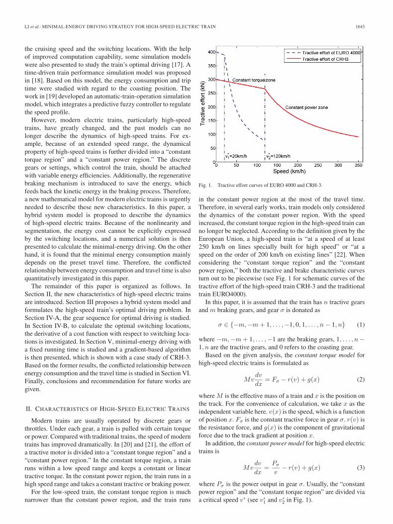
Fig. 1. Tractive effort curves of EURO 4000 and CRH-3.

in the constant power region at the most of the travel time.Therefore, in several early works, train models only consideredthe dynamics of the constant power region. With the speedincreased, the constant torque region in the high-speed train canno longer be neglected. According to the definition given by theEuropean Union, a high-speed train is “at a speed of at least250 km/h on lines specially built for high speed” or “at aspeed on the order of 200 km/h on existing lines” [22]. Whenconsidering the “constant torque region” and the “constantpower region,” both the tractive and brake characteristic curvesturn out to be piecewise (see Fig. 1 for schematic curves of thetractive effort of the high-speed train CRH-3 and the traditionaltrain EURO4000).

In this paper, it is assumed that the train has n tractive gearsand m braking gears, and gear σ is donated as

σ ∈ {−m,−m+ 1, . . . ,−1, 0, 1, . . . , n− 1, n} (1)

where −m,−m+ 1, . . . ,−1 are the braking gears, 1, . . . , n−1, n are the tractive gears, and 0 refers to the coasting gear.

Based on the given analysis, the constant torque model forhigh-speed electric trains is formulated as

Mvdv

dx= Fσ − r(v) + g(x) (2)

where M is the effective mass of a train and x is the position onthe track. For the convenience of calculation, we take x as theindependent variable here. v(x) is the speed, which is a functionof position x. Fσ is the constant tractive force in gear σ. r(v) isthe resistance force, and g(x) is the component of gravitationalforce due to the track gradient at position x.

In addition, the constant power model for high-speed electrictrains is

Mvdv

dx=

Pσ

v− r(v) + g(x) (3)

where Pσ is the power output in gear σ. Usually, the “constantpower region” and the “constant torque region” are divided viaa critical speed v∗ (see v∗1 and v∗2 in Fig. 1).


To evaluate the energy consumption of the given driving sce-nario, there are usually two kinds of energy flows that need to beconsidered, i.e., the output energy and the feedback energy. Theoutput energy can be further divided into the energy consumedin a propulsion system, the energy used in auxiliary machin-ery, and the energy losses in ventilation, air conditioning,lighting, and toilets. As the latter two terms are approximatelyconstants and minor, the energy consumed in propulsion ismerely considered in this paper, which accounts for the largestpartition in output energy. The energy consumption in propul-sion consists of the energy loss in aerodynamic resistance andthe energy stored in a train, including potential energy andkinetic energy. When the train runs from position x1 withspeed v1 to position x2 with speed v2, the energy consumedin propulsion can be expressed as

ΔJ =

x2∫x1

r(v)dx−x2∫

x1

g(x)dx+12M(v22 − v21

). (4)

The tractive motor of a train usually has an optimal operatingregion [23] and the energy efficiency changes with respectto different operation conditions [24]. In some literature, theefficiency of propulsion is taken as a constant coefficient, suchas in [16] and [25]. The work in [26] investigated the factorsaffecting the energy efficiency of electric trains, which includethe speed and the rates of acceleration and deceleration. Sim-ilarly, in [9] and [27], the energy efficiency of a train is ex-pressed as a function of tractive force and speed. More tractiveefforts and a higher speed always cause higher energy effi-ciency. In practice, the energy efficiency is an important factorconsidered when designing the driving strategy. There are someother factors affecting the energy efficiency of a propulsion sys-tem, such as load, acceleration, etc. In this paper, it is assumedthat the energy efficiency only depends on the gear and speed.Therefore, the energy consumption in (4) should be modified as

ΔJ =

x2∫x1

F/α(σ, v)dx. (5)

Here, energy efficiency factor α(σ, v) is a function of gear σand speed v, and takes a value between 0 and 1.

For the sake of energy saving, most electric trains areequipped with a regenerative brake [28]. When braking, thetraction motor works in generator mode. The kinetic energyof a wheel is translated into electrical energy, which is thenfed back into the electricity net or stored into the onboardbattery. Similarly, the recovering efficiency of the regenerativebrake also depends on brake effort and speed (for the detailedcharacteristics, see [6] and [29]). The feedback energy in theregenerative brake can be formulated as a function of gear andspeed, i.e.,

ΔJ =

x2∫x1

β(σ, v)Fdx. (6)

Here, recovering factor β(σ, v) represents the percentage offeedback energy accounting for the total brake energy.

Remark 1: For the symbol’s unification, the tractive forceand the brake force are donated with the same symbol F in(4)–(6). In practice, F should be substituted with Pσ/v inthe constant power region and with Fσ in the constant torqueregion. When in traction, F takes a positive value and the outputpower is also positive. When in regenerative braking, F takes anegative value and the energy in (6) is negative. In this case, thefeedback energy should be comprehended as a negative outputenergy.

In summary, the four new characteristics considered forhigh-speed electric trains are: 1) the discrete-gear operatingmechanism; 2) the dynamics of model autonomously switchingbetween the “constant torque region” and the “constant powerregion”; 3) energy efficiency changing with respect to gearsand speed; and 4) the regenerative brake attached with energyfeedback.

III. HYBRID SYSTEM MODEL AND

PROBLEM FORMULATION

Here, a hybrid system model is introduced to cover thenew characteristics of a high-speed electric train. The hybridsystem is a dynamic system that exhibits both continuous anddiscrete dynamic behaviors [30], [31], in which the continuousdynamics are governed by a differential equation and the dis-crete dynamics are described by a logical graph. In [32] and[33], the dynamics of an electric train are modeled with a hybridsystem, in which the dynamics of the train is simplified into alinear relationship and the control variables are the gear angle,the manifold pressure in continuous form, and the gear positionin discrete form.

Typically, an extended automaton is proposed to representthe hybrid system, i.e., a hybrid automaton (HA) [34]. In thispaper, a special HA is defined for a high-speed train. It is a six-tuple collection as follows:

H = {D,C, f, I, S,G} (7)

where

• D = {σ} is the set of operation modes. To distinguish thedynamics of the constant torque region and the constantpower region, the gears in (1) are split as follows:

σ ∈ {−mct,−mcp,−(m− 1)ct,−(m− 1)cp, . . . ,−1ct,

−1cp, 0, 1ct, 1cp, . . . , (n− 1)ct, (n− 1)cp, nct, ncp} .

• C = {v, t}is the set of the continuous states, which con-sists of speed v and travel time t. Position x is taken as theindependent variable here.

• f : D × C → TC is the vector field, which governs theevolution of the continuous states. Referring to the differ-ential equations (3) and (2), f should be a function vectorf = [f1, f2]

T formulated as

{dvdx = f1(σ, v) =

1Mv (Fσ − r(v) + g(x))

dtdx = f2(σ, v) =

1v

(8)


Fig. 2. HA for high-speed trains. The hard arrow is the controlled switching,and the dashed arrow is the autonomous switching. v∗t and v∗b are the criticalspeeds for tractive and braking efforts, respectively.

or {dvdx = f1(σ, v) =

1Mv

(Pσ

v − r(v) + g(x))

dtdx = f2(σ, v) =

1v .

(9)

• I ⊆ D × C are the initial states of the train, including thecontinuous states and discrete modes.

• S ⊆ D ×D is the allowable switch between operationmodes. For high-speed train driving, the allowable switchconsists of the controlled switches between gears and theautonomous switches between the constant torque regionand the constant power region. In addition, the switch isassumed to be taking no time, but the Zeno behavior is notconsidered here.

• G : S → P (C) is the guard condition for switch S, whichis usually a hyperplane on C. As there is autonomousswitching between the constant torque mode and the con-stant power mode, the guard condition is the threshold ofthe critical speed v∗.

Typically, for an HA with a discontinuous switch, a reset termis introduced to update the state value after switching [35]. Asthe states of the train are continuous throughout the operationmode switching, the reset term is neglected here. (See Fig. 2 foran illustration of mode switching.)

As the autonomous switches between the constant torqueregion and the constant power region are mutually exclusive,the discrete state of the train is represented by gear σ only inthe following content. For a certain driving, the gear sequenceis donated as

Σ = {σ0, σ1, . . . , σi, . . . , σN} (10)

where σi denotes the ith gear in the gear sequence and Nis the number of switching gears. If the gear switching doesnot involve energy consumption, more gear switching resultsin better driving because it can arbitrarily control the speedcurve with no cost. Obviously, this is not practical. In someliterature, each gear switching is attached with a penalty cost.In this paper, the switching number is fixed with N . Moreover,the corresponding switching location sequence is

Γ = {x0, x1, . . . , xi, . . . , xN} (11)

with x0 = 0, xN = X . X is the length of a journey. Gear σi isactive in interval [xi−1, xi]. Therefore, a trajectory to the HA in(7) can be written as

ρ : (σ0, vx0, tx0

) �→ (σ1, vx1, tx1

) �→ · · · (σN , vxN, txN

).(12)

In practice, there are some constraints for train running. Atfirst, the initial states of the train are fixed with

σ0 = 0 v(x0) = 0 t(x0) = 0. (13)

The running speed is limited by

v(x) ≤ Vmax(x) (14)

where Vmax(x) is the maximum permissible speed atposition x.

Obviously, the train must stop at the destination station witha given travel time, i.e.,

v(xN ) = 0 t(xN ) = T (15)

where T is the prespecified travel time.Now, the following cost function is adopted to evaluate the

energy consumption:

J =

N∑i=1

xi∫xi−1

Lσi(v, x)dx. (16)

Lσ is a piecewise function, i.e.,

Lσi=

⎧⎪⎨⎪⎩

Fσi/α(σi, v), σi ≥ 0; v ≤ vt∗

Pσi/v/α(σi, v), σi ≥ 0; v ≥ vt∗

β(σi, v)Fσi, σi < 0; v ≤ vb∗

β(σi, v)Pσi/v, σi < 0; v ≥ vb∗

(17)

where α(σi, v) is the traction energy efficiency in (5) andβ(σi, v) is the regenerative energy efficiency in (6). vt∗ is thecritical speed of traction and vb∗ is the critical speed of braking(see Fig. 2).

Finally, the minimal-energy driving problem for high-speedelectric trains can be formally formulated as follows.

Problem 1: Find the switching gear sequence Σ and switch-ing locations Γ to make the cost function J in (16) minimal,which is subjected to constraints in (7), (13)–(15).

IV. SOLUTION

The given problem can be comprehended as the optimalcontrol for the hybrid system with autonomous switching. Thework in [36] presented a unified framework for optimal controlof the hybrid system. In [37], the existence of optimal controlfor the hybrid system is analyzed with the MP. In this paper, asthe length of the gear sequence is fixed and switching locationsare in a closed interval, the existence of optimal driving is nodoubt. In [38], a two-stage technology is proposed as follows:1) Study the traditional optimal control problem with fixeddiscrete control sequence and find the switching instants andoptimal control and 2) change the previous discrete controlsequence and repeat step 1. Obviously, after searching allpossible discrete sequences, the optimal driving strategy willbe determined.

However, when adopting the given technology, the computa-tion complexity will be intolerable. For driving, there are (n+m+ 1)N possible gear sequences; therefore, the calculationamount is exponential with the length of the gear sequence.


Fig. 3. Balance speeds of gears.

To avoid searching blindly for the space of the switchingsequence, the gear sequence should be determined with a prioriknowledge.

A. Gear Sequence

As aforementioned, the driving process can be divided intofour stages, namely, traction, cruising, coasting, and braking.The following will analyze each stage and determine the gearsequence.

1) Cruising Stage: In the cruising stage, the train keeps aconstant speed Vc. Usually, the constant speed is implementedvia switching between two operation modes. For example, thecruising stage consists of maximum traction and coasting in[39]. For the high-speed train in this paper, constant speed Vc

can be kept by switching between σ and σ + 1 gears with

Fσ(Vc) ≤ r(Vc) + g(x) ≤ Fσ+1(Vc) (18)

where Fσ(Vc) is the traction effort under gear σ and speed Vc.In fact, this strategy is only suitable for a freight train. For

passenger trains, frequent switching between throttles σ andσ + 1 makes the comfort poor. Therefore, it is sensible tochoose a constant gear in the cruising stage. For each gear σ,there always exists balanced speed Vσ as follows:

{Vσ | Fσ(Vσ)− r(Vσ) + g(x) = 0} . (19)

Therefore, the cruising speed is equal to balanced speed. (SeeFig. 3 for balance speeds of the train with four gears.)

When the cruising stage dominates the trip time, cruisinggear σ∗ can be determined, whose balance speed is just greaterthan the average speed, i.e.,

{σ∗ | Vσ∗−1 ≤ X/T ≤ Vσ∗} (20)

where trip time T and trip length X are given.2) Traction Stage: In the traction stage, the train is accel-

erated to the cruising speed. Usually, there are two kinds ofacceleration strategies. The first strategy switches traction gears

from gear 1 to gear n with ascending order, which acceleratesthe train blandly and is good for the health of the train, buttakes more time to reach the cruising speed. The other strategyaccelerates the train from maximum traction gear n to gear 1.Of course, the advantage of this strategy is rapid, but the hugeinitial accelerator can destroy the train’s health.

To investigate the two kinds of strategies, a mixed tractionstrategy is proposed here, which first adopts an ascending orderof switching from gear 1 to gear n and then switches from gearn to cruising gear σ∗ with descending order, i.e.,

Σt = {1, 2, . . . , n− 1, n, n− 1, . . . , σ∗}. (21)

3) Braking Stage: There are two kinds of braking mecha-nisms in an electric train, i.e., regenerative braking and me-chanical braking. The former is suitable for a high speed range,which translates the kinetic energy into electricity and thenstores it. The latter is used for low speed without energy feed-back. As a higher braking gear usually has higher efficiency ofenergy feedback, a descending-order braking strategy is takenhere, i.e.,

Σb = {−m,−m+ 1, . . . ,−1}. (22)

Once the gear sequence Σ is fixed, cost function J onlydepends on switching locations Γ, i.e.,

J(x0, x1, . . . , xN ) =

N∑i=1

xi∫xi−1

Lσi(x, v)dx. (23)

This is a nonlinear optimization problem. An exterior pointmethod based on gradient information will be an option tocalculate the optimal switching locations under a given gearsequence. Now, the gradient of the cost function with respectto locations is denoted as

dJ

dΓ=

[∂J

∂x1,∂J

∂x2, . . . ,

∂J

∂xN−1

]T. (24)

Here, the terminal conditions are fixed, i.e., x0 = 0 andxN = X .

If we can obtain the explicit expression of the cost functionwith respect to locations, the gradient dJ/dΓ can be deducedanalytically. However, from the differential equation of theconstant power region in (3), only a hidden expression of speedand position can be obtained as

x−v(x)∫0

τ2

Pσ − aτ − bvτ − cτ3dτ + C1 = 0 (25)

where a, b, and c are fixed parameters, and C1 depends on theinitial values. Obviously, it is impossible to derive an explicitexpression of the cost function from (23) and (25).


Fig. 4. Variational of the speed profile.

B. Derivation of the Switching Locations

Here, an approximate gradient information dJ/dΓ will becalculated for the exterior point method. First, formulate thecost function on [xi, xi+1] as

Ji =

xi+1∫xi

Lσi(x, v)dx. (26)

Therefore, the total cost is

J =N−1∑i=0

Ji =N−1∑i=0

xi+1∫xi

Lσi(x, v)dx. (27)

According to (8) and (9), the speed evolution is reformulated as

dv

dx= f1(σi, v, x), x ∈ [xi, xi+1]. (28)

In the following content, the variational method is adopted tocalculate the partial derivative ∂J/∂xi. First, given a positivedisturbance Δxi to switching location xi, this disturbance willcause a new speed profile, which is denoted as v [see Fig. 4(a)].

In [xi, xi +Δxi], write the Taylor expansion of the newspeed profile as

v(x) = v(xi) + f1(σi, v(xi), x)(x− xi) + o(x− xi). (29)

The corresponding variation to the speed profile is

δv(x) = v(x)− v(x)

= v(x)− (v(xi) + f1 (σi+1, v(xi), x)

× (x− xi) + o(x− xi))

= [f1 (σi, v(xi), x)− f1(σi+1, v(xi), x)]

× (x− xi) + o(x− xi) (30)

and the speed change at xi +Δx is

δv(xi +Δx) = [f1 (σi, v(xi), x)

−f1 (σi+1, v(xi), x)]Δx+ o(x− xi). (31)

In [xi +Δxi, xi+1], the differential equation for speed evo-lution is

dv

dx= f1(σi+1, v, x). (32)

In addition, the variation of speed can be expressed in a differ-ential equation as

d(δv)

dx= f1(σi+1, v, x)− f1(σi+1, v, x)

=∂f1(σi+1, v, x)

∂v(v − v) + o(v − v)

∂f1(σi+1, v, x)

∂vδv. (33)

Let us introduce a state transition function Tk(x1, x2) for dif-ferential equation (d(δv)/dx) = (∂f1(σk+1, v, x)/∂v)δv, k =i, . . . , N − 1 as follows:

δv(x2) = δv(x1)Tk(x1, x2), xk ≤ x1 ≤ x2 ≤ xk+1.(34)

The speed variable in (33) can be formulated as

δv(x)=δv(xi+Δxi)Ti(xi+Δxi, x), x ∈ [xi+Δxi, xi+1](35)

and for k = i+ 1, . . . , N − 1, we have

δv(x) = δv(xk)Tk(xk, x), x ∈ [xk, xk+1]. (36)

The cost function can be rewritten as

J =

N−1∑j=0

Jj

=

N−1∑j=0, j =i

xj+1∫xj

Lσj(x, v)dx+

xi+Δxi∫xi

Lσi(x, v)dx

+

xi+1∫xi+Δxi

Lσi+1(x, v)dx. (37)

Then, we expand it at the original speed profile v(x) with theTaylor series and obtain the disturbance of cost in (38). Accord-ing to (31) and (36), when we take Δxi → 0, the disturbance ofcost in (38) can be expressed as (39), as shown in

ΔJ = J − J

=

xi+Δxi∫xi

(∂Lσi

∂v− 2

∂Lσi+1

∂v

)δvdx

+N−1∑j=i

⎧⎪⎨⎪⎩

xj+1∫xj

∂Lσj+1

∂vδvdx

⎫⎪⎬⎪⎭+ o(δv) (38)


=

(∂Lσi

∂v− 2

∂Lσi+1

∂v

)δvΔxi

+

N−1∑j=i

⎧⎪⎨⎪⎩

xj+1∫xj

∂Lσj+1

∂vδvdx

⎫⎪⎬⎪⎭+ o(Δxi) (Δxi→0)

= (f1 (σi, v(xi), x)− f1 (σi+1, v(xi), x))

×Δx

(N−1∑j=i

xj+1∫xj

∂Lσj+1

∂v

(Πj−1

k=iTk(xk, xk+1))

× Tj(xj , x)dx

)+ o(Δxi) (39)

(f1 (σi, v(xi), x)− f1 (σi+1, v(xi), x))

×Δx

xi+1∫xi

(∂Lσi+1

∂vTi(xi, x)

)dx+ o(Δxi). (40)

In practice, the disturbance of speed in (36) always decaysdramatically. An approximate expression for the disturbance ofspeed is

δv(x) =

{δv(xi +Δxi)Ti(xi, x), x ∈ [xi, xi+1]0, x ∈ [xi+1, xN ]

(41)

and the disturbance of cost in (39) can be further simplified asin (40).

Finally, the derivative of the cost function with respect to theswitching locations xi can be approximately formulated as

∂J

∂xi= [f1 (σi, v(xi), x)− f1 (σi+1, v(xi), x)]

×xi+1∫xi

∂Lσi+1

∂vTi(xi, x)dx (42)

where i = 0, N as the initial and terminal instants are fixed. Inaddition, the second-order gradient information ∂2J/∂2xi canalso be calculated based on the given result (see [40]).

V. OPTIMAL DRIVING WITH FIXED TRAVEL TIME

For optimal driving, there still are three constraints to besatisfied, namely, initial constraints in (13), speed limitation in(14), and the terminal condition in (15). Given trip time T , weextend the cost function in (16) as

JE =

N∑i=1

xi∫xi−1

Lσ(v, x)dx+ γ

⎛⎜⎝ N∑

i=1

xi∫xi−1

1vdx− T

⎞⎟⎠

2

. (43)

Here, γ is a penalty factor that can force the speed profile tosatisfy the trip time constraint.

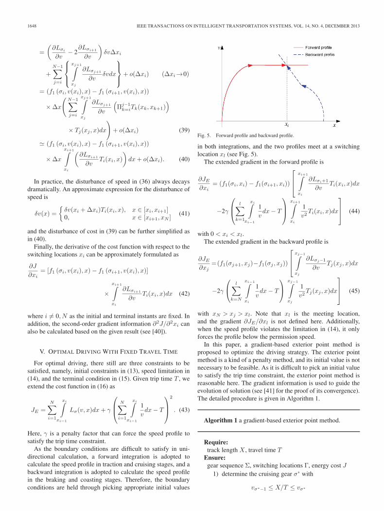
As the boundary conditions are difficult to satisfy in uni-directional calculation, a forward integration is adopted tocalculate the speed profile in traction and cruising stages, and abackward integration is adopted to calculate the speed profilein the braking and coasting stages. Therefore, the boundaryconditions are held through picking appropriate initial values

Fig. 5. Forward profile and backward profile.

in both integrations, and the two profiles meet at a switchinglocation xl (see Fig. 5).

The extended gradient in the forward profile is

∂JE∂xi

= (f1(σi, xi)− f1(σi+1, xi))

⎡⎢⎣

xi+1∫xi

∂Lσi+1

∂vTi(xi, x)dx

−2γ

⎛⎜⎝ l∑

k=1

xi∫xi−1

1vdx− T

⎞⎟⎠

xi+1∫xi

1v2

Ti(xi, x)dx

⎤⎥⎦ (44)

with 0 < xi < xl.The extended gradient in the backward profile is

∂JE∂xj

=(f1(σj+1, xj)−f1(σj , xj))

⎡⎢⎣

xj−1∫xj

∂Lσj−1

∂vTj(xj , x)dx

−2γ

⎛⎝ l∑

k=N

xi−1∫xi

1vdx− T

⎞⎠ xj−1∫

xj

1v2

Tj(xj , x)dx

⎤⎥⎦ (45)

with xN > xj > xl. Note that xl is the meeting location,and the gradient ∂JE/∂xl is not defined here. Additionally,when the speed profile violates the limitation in (14), it onlyforces the profile below the permission speed.

In this paper, a gradient-based exterior point method isproposed to optimize the driving strategy. The exterior pointmethod is a kind of a penalty method, and its initial value is notnecessary to be feasible. As it is difficult to pick an initial valueto satisfy the trip time constraint, the exterior point method isreasonable here. The gradient information is used to guide theevolution of solution (see [41] for the proof of its convergence).The detailed procedure is given in Algorithm 1.

Algorithm 1 a gradient-based exterior point method.

Require:track length X , travel time T

Ensure:gear sequence Σ, switching locations Γ, energy cost J

1) determine the cruising gear σ∗ with

vσ∗−1 ≤ X/T ≤ vσ∗


2) fix the initial gear sequence

Σ = {1, . . . , n, n− 1, . . . , σ∗,−m,−m+ 1, . . . ,−1}

3) initialize the switching locations and iterative label k

Γ0 = [x1, x2, . . . , xN−1]T , k = 0

4) solve speed profiles using a fourth-order Runge–Kuttamethod• forward profile in [x0, xl] with v(x0) = 0• vi(x)=ode45(fσi

, [xi−1, xi], v(xi−1)) , i=1, . . . , l• backward profile in [xl, xN ] with v(xN ) = 0• vj(x) = ode45(fσj

, [xj , xj−1], v(xj)), j = N, . . . ,l + 1

5) calculate the gradient information with (44), (45)

dJEdΓk

=

[∂JE∂x1

,∂JE∂x2

, . . . ,∂JE

∂xN−1

]T

6) update the switching locations

Γk+1 = Γk + h

(dJEdΓk

)T

7) get the cost function Jk+1 with (43)8) evaluate the terminal condition∣∣∣∣Jk+1 − Jk

Jk+1

∣∣∣∣ ≤ δ

9) repeat10) steps 4, 5, 6, 7, and 811) until the terminal condition is satisfied12) return Σ, Γ, J

Remark 2: As the magnitude values of the energy term andthe time term in the cost function are dramatically mismatched,the gradient-based algorithm proposed here may oscillate se-riously. First, a large initial penalty factor γ can quickly forcethe speed profile to satisfy the journey time constraint. Then,the energy consumption is minimized with an increased penaltyfactor. Therefore, the penalty factor in this algorithm should notbeen tuned in a strictly increasing order.

Remark 3: In this algorithm, the gear sequence is fixed witha priori knowledge of train driving. In fact, it can also calculatethe optimal switching locations for an arbitrary feasible gearsequence.

A. Case Study

Here, the optimal driving for the high-speed electric trainCRH-3 is studied, which is a version of the Siemens Velarohigh-speed train used in China. A track interval is chosen on theBeijing–Tianjin Intercity Railway with length L = 72 km andthe travel time is fixed as T = 1200 s. The main parameters of

TABLE IPARAMETERS OF CRH-3

TABLE IIPARAMETERS OF GEARS

CRH-3 are listed in Table I. The maximum tractive and brakingforces are

Fmt =

{300 − 0.284v 0 ≤ v ≤ 119.7 km/h266 × 119.7/v 119.7 ≤ v ≤ 300 km/h

(kN)

Fmb =

{−300 + 0.281v 0 ≤ v ≤ 106.7 km/h−270 × 106.7/v 106.7 ≤ v ≤ 300 km/h

(kN).

The resistant and frictional forces are summarized in the termr(v). The frictional force is mainly an adhesive force caused bythe contact between the wheel and the track surface, and theresistance consists of bearing or resistance, flange resistance,and aerodynamic resistance. Here, we adopt the experientialexpression in [16] as

r(v)=6.4M+130q+0.14Mv+[0.046+0.0065(p−1)]Av2

(46)

where M is the actual mass in tons, q is the number of axles,p is the number of cars in the train, and A is the frontal area insquare meters. Substituting the parameters of CRH-3 in Table Iinto (46), the sum of the resistant and frictional forces can beexpressed as

r(v) = 6774.4 + 57.19v + 0.8235v2 (47)

where v is the speed in kilometers per hour and r(v) is theresistance in newtons.

In practice, the gear number of a high-speed train is morethan 8 or even 13. For simplification of computation, it isassumed that the high-speed train works in four tractive gearsand four braking gears. The properties of each gear are shownin Table II. Fmt is the maximum tractive force and Fmb is


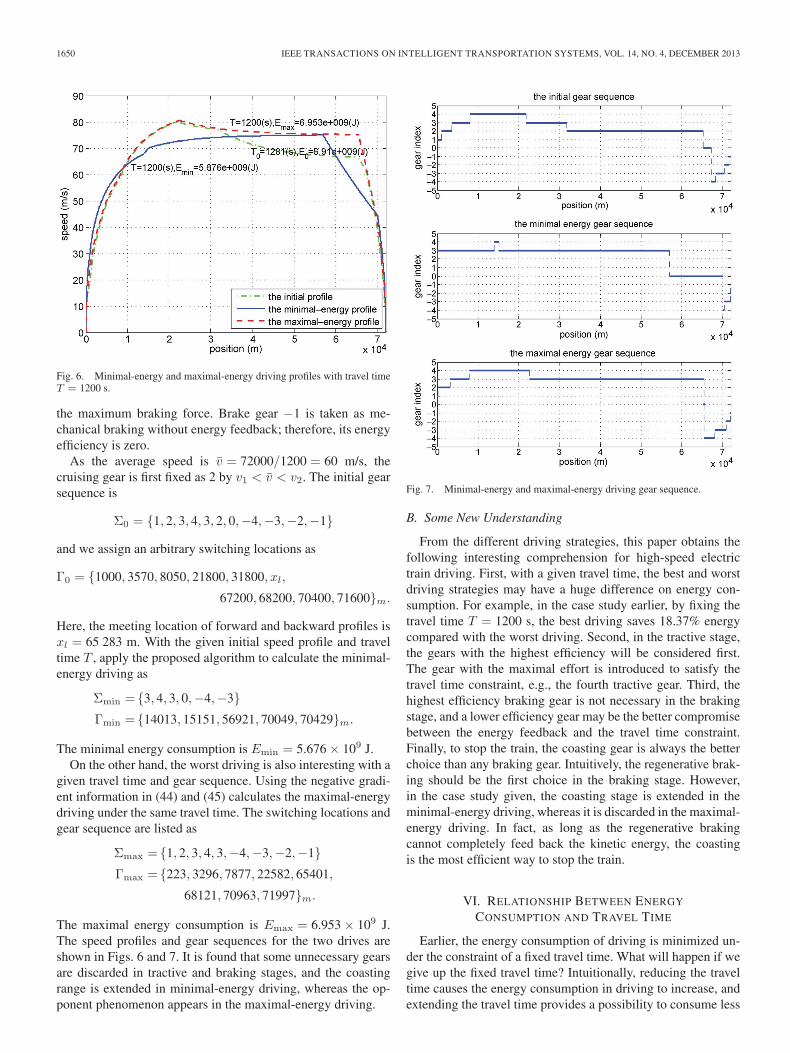
Fig. 6. Minimal-energy and maximal-energy driving profiles with travel timeT = 1200 s.

the maximum braking force. Brake gear −1 is taken as me-chanical braking without energy feedback; therefore, its energyefficiency is zero.

As the average speed is v = 72000/1200 = 60 m/s, thecruising gear is first fixed as 2 by v1 < v < v2. The initial gearsequence is

Σ0 = {1, 2, 3, 4, 3, 2, 0,−4,−3,−2,−1}

and we assign an arbitrary switching locations as

Γ0 = {1000, 3570, 8050, 21800, 31800, xl,

67200, 68200, 70400, 71600}m.

Here, the meeting location of forward and backward profiles isxl = 65 283 m. With the given initial speed profile and traveltime T , apply the proposed algorithm to calculate the minimal-energy driving as

Σmin = {3, 4, 3, 0,−4,−3}Γmin = {14013, 15151, 56921, 70049, 70429}m.

The minimal energy consumption is Emin = 5.676 × 109 J.On the other hand, the worst driving is also interesting with a

given travel time and gear sequence. Using the negative gradi-ent information in (44) and (45) calculates the maximal-energydriving under the same travel time. The switching locations andgear sequence are listed as

Σmax = {1, 2, 3, 4, 3,−4,−3,−2,−1}Γmax = {223, 3296, 7877, 22582, 65401,

68121, 70963, 71997}m.

The maximal energy consumption is Emax = 6.953 × 109 J.The speed profiles and gear sequences for the two drives areshown in Figs. 6 and 7. It is found that some unnecessary gearsare discarded in tractive and braking stages, and the coastingrange is extended in minimal-energy driving, whereas the op-ponent phenomenon appears in the maximal-energy driving.

Fig. 7. Minimal-energy and maximal-energy driving gear sequence.

B. Some New Understanding

From the different driving strategies, this paper obtains thefollowing interesting comprehension for high-speed electrictrain driving. First, with a given travel time, the best and worstdriving strategies may have a huge difference on energy con-sumption. For example, in the case study earlier, by fixing thetravel time T = 1200 s, the best driving saves 18.37% energycompared with the worst driving. Second, in the tractive stage,the gears with the highest efficiency will be considered first.The gear with the maximal effort is introduced to satisfy thetravel time constraint, e.g., the fourth tractive gear. Third, thehighest efficiency braking gear is not necessary in the brakingstage, and a lower efficiency gear may be the better compromisebetween the energy feedback and the travel time constraint.Finally, to stop the train, the coasting gear is always the betterchoice than any braking gear. Intuitively, the regenerative brak-ing should be the first choice in the braking stage. However,in the case study given, the coasting stage is extended in theminimal-energy driving, whereas it is discarded in the maximal-energy driving. In fact, as long as the regenerative brakingcannot completely feed back the kinetic energy, the coastingis the most efficient way to stop the train.

VI. RELATIONSHIP BETWEEN ENERGY

CONSUMPTION AND TRAVEL TIME

Earlier, the energy consumption of driving is minimized un-der the constraint of a fixed travel time. What will happen if wegive up the fixed travel time? Intuitionally, reducing the traveltime causes the energy consumption in driving to increase, andextending the travel time provides a possibility to consume less


Fig. 8. Relationship of journey time T and energy consumption E.

energy in driving. The work in [42] first discusses the conflictedrelationship between energy consumption and travel time, andthen introduces the Pareto efficiency into train driving. In[43], Pareto curves for high-speed train driving are investigatedvia computer simulation. In addition, the tradeoff relationshipin train driving is investigated in [44]. Here, we investigatethe quantitative relationship between energy consumption andtravel time.

In general, it is difficult to get an analytical expressionbetween energy consumption and travel time on a given track.Among the four stages of the driving process, the cruisingstage usually consumes most of the energy on a long track,whereas the energy consumption of the other three stages arerelatively constant. When denoting the length of the cruisingstage as Xc and its running time as Tc, the average speed incruising is

Vc =Xc

Tc. (48)

In the cruising stage, the energy is mainly used to resist forcer(v). Therefore, the energy consumption in the cruising stagecan be expressed as

Ec = r(Vc)Xc. (49)

When the track line is long enough, it is reasonable to use (48)and (49) to approximately express the conflicted relationshipbetween energy consumption and travel time on the wholeline, i.e.,

E = r

(X

T

)X. (50)

For example, taking the r(v) in (47), the energy consumptionof CRH-3 can be expressed as (see Fig. 8)

E = 6774.4X + 205.88X2

T+ 10.67

X3

T 2. (51)

It turns out that energy consumption is a hyperbolic functionof travel time, which means that the energy cost increases foreach reduced unit of travel time. It is very useful to introducethe concept of marginal power to measure the energy cost oftravel time cutting, which is defined as the energy consumptionfor every second cut in travel time, i.e.,

Pm =ΔE

ΔT. (52)

Based on (51), the marginal power for CRH-3 can be approxi-mately formulated as

Pm(T ) = −205.88X2

T 2− 21.34

X3

T 3. (53)

This is similar to the marginal benefit in economics. Fromthe passengers’ perspective, shortening the travel time is alwaysa good thing. However, unwisely reducing the travel time isunreasonable in some situation because the energy consumptionmay sharply increase with respect to each unit of travel time cut.On the other hand, a train operator always intends to extendtravel time to save energy. With the help of marginal power, itis possible to evaluate the energy cost of changing the recenttravel time and to find a tradeoff scheme.

VII. CONCLUSION

In this paper, the optimal driving for high-speed electrictrains has been investigated. A hybrid system model for trainsis presented to satisfy the new properties of high-speed electrictrains, which includes the extended speed range, the operatedgears with energy efficiencies, and regenerative braking. Withthe gear sequence fixed by a priori knowledge, the optimaldriving for the high-speed electric train turns out to be anonlinear optimization problem. Because there is no explicitexpression of energy cost with respect to switch locations, anexterior point method is proposed to calculate the minimal- andmaximal-energy driving strategies. In the minimal-energy driv-ing, the most efficient gear dominates the tractive and cruisingstages, whereas the highest speed gear is adopted to satisfy thetravel time constraint. Contrary to the intuitive understanding,coasting is more efficient than regenerative braking in the casestudy. At last, the concept of marginal power is introduced toevaluate the efficiency of changing the travel time. A reasonabletravel time is definitely the best way to save energy in high-speed train driving. There are still some future works abouthigh-speed train driving. For example, this paper just treatsthe energy efficiency as the constant values because of thebottleneck of computation amount. An efficient and powerfuloptimization algorithm is urgently needed in the future.

REFERENCES

[1] S. Kobayashi, S. Plotkin, and S. K. Ribeiro, “Energy efficiency technolo-gies for road vehicles,” Energy Efficiency, vol. 2, no. 1, pp. 125–137,May 2009.

[2] I. Kunihiko, “Application of optimization theory for bounded state vari-able problems to the operation of train,” Bull. Jpn. Soc. Mech. Eng.,vol. 11, no. 47, pp. 857–865, Nov. 1968.

[3] I. A. Asnis, A. V. Dmitruk, and N. P. Osmolovskii, “Solution of theproblem of the energetically optimal-control of the motion of a train by


the maximum principle,” USSR Comput. Math. Math. Phys., vol. 25, no. 6,pp. 37–44, 1985.

[4] E. Khmelnitsky, “On an optimal control problem of train operation,” IEEETrans. Autom. Control, vol. 45, no. 7, pp. 1257–1266, Jul. 2000.

[5] R. Liu and I. M. Golovitcher, “Energy-efficient operation of rail vehicles,”Transp. Res. Part A, Policy Pract., vol. 37, no. 10, pp. 917–932, Dec. 2003.

[6] M. Miyatake and H. Ko, “Optimization of train speed profle for minimumenergy consumption,” IEEJ Trans. Elect. Electron. Eng., vol. 5, no. 3,pp. 263–269, May 2010.

[7] H. Ko, T. Koseki, and M. Miyatake, “Application of dynamic program-ming to the optimization of the running profile of a train,” in Computersin Railway SIX. Southampton: WIT Press, 2004, pp. 103–112.

[8] W. S. Lin and J. W. Sheu, “Automatic train regulation for metro lines usingdual heuristic dynamic programming,” Proc. Inst. Mech. Eng. Part F,J. Rail Rapid Transit, vol. 224, no. F1, pp. 15–23, Jan. 2010.

[9] R. Franke, P. Terwiesch, and M. Meyer, “An algorithm for the optimalcontrol of the driving of trains,” in Proc. 39th IEEE Conf. DecisionControl, 2000, vol. 3, pp. 2123–2128.

[10] J. X. Cheng and P. Howlett, “Application of critical velocities to theminimization of fuel consumption in the control of trains,” Automatica,vol. 28, no. 1, pp. 165–169, Jan. 1992.

[11] P. G. Howlett, I. P. Milroy, and P. J. Pudney, “Energy-efficient traincontrol,” Control Eng. Pract., vol. 2, no. 2, pp. 193–200, Apr. 1994.

[12] P. G. Howlett, P. J. Pudney, and X. Vu, “Local energy minimizationin optimal train control,” Automatica, vol. 45, no. 11, pp. 2692–2698,Nov. 2009.

[13] X. Vu, “Analysis of necessary conditions for the optimal control of atrain,” Ph.D. dissertation, Univ. South Australia, Adelaide, SA, Australia,2006.

[14] G. Acampora, C. Landi, M. Luiso, and N. Pasquino, “Optimization ofenergy consumption in a railway traction system,” in Proc. SPEEDAM,2006, pp. 1121–1126.

[15] B.-R. Ke, C.-L. Lin, and C.-W. Lai, “Optimization of train-speed trajec-tory and control for mass rapid transit systems,” Control Eng. Pract.,vol. 19, no. 7, pp. 675–687, Jul. 2011.

[16] K. Kim and S. I.-J. Chien, “Optimal train operation for minimum energyconsumption considering track alignment, speed limit, and schedule ad-herence,” J. Transp. Eng., vol. 137, no. 9, pp. 665–674, Sep. 2011.

[17] C. J. Goodman, L. K. Siu, and T. K. Ho, “A review of simulation modelsfor railway systems,” in Proc. Int. Conf. Dev. Mass Transit Syst., London,U.K., 1998, pp. 80–85.

[18] K. Kim and S. I.-J. Chien, “Simulation-based analysis of train controls un-der various track alignments,” J. Transp. Eng., vol. 136, no. 11, pp. 937–948, Nov. 2010.

[19] S. Yasunobu and S. Miyamoto, “Automatic train operation system bypredictive fuzzy control,” in Industrial Applications of Fuzzy control.Amsterdam, The Netherlands: Elsevier, 1985, pp. 1–18.

[20] S. Lu, S. Hillmansen, and C. Roberts, “A power-management strategy formultiple-unit railroad vehicles,” IEEE Trans. Veh. Technol., vol. 60, no. 2,pp. 406–420, Feb. 2011.

[21] F. Schmid and C. J. Goodman, “Electric railway systems in common use,”in Proc. 5th IET Professional Dev. Course REIS, 2011, pp. 1–15.

[22] General definitions of highspeed 2009.[23] K. T. Chau and Y. S. Wong, “Overview of power management in hybrid

electric vehicles,” Energy Convers. Manage., vol. 43, no. 15, pp. 1953–1968, Oct. 2002.

[24] J. Faiz and M. B. B. Sharifian, “Optimal design of an induction motor foran electric vehicle,” Eur. Trans. Elect. Power, vol. 16, no. 1, pp. 15–33,Jan. 2006.

[25] W. W. Hay, Railroad Engineering, 2nd ed. New York, NY, USA: Wiley,1982.

[26] N. Iwai, “Analysis on fuel economy and advanced systems of hybridvehicles,” JSAE Rev., vol. 20, no. 1, pp. 3–11, Jan. 1999.

[27] J. C. Jong and E. F. Chang, “Models for estimating energy consumptionof electric train,” J. Eastern Asia Soc. Transp. Stud., vol. 6, pp. 278–291,2005.

[28] M. Miyatake and H. Ko, “Numerical analyses of minimum energy opera-tion of multiple trains under dc power feeding circuit,” in Proc. Eur. Conf.Power Electron. Appl., 2007, pp. 1–10.

[29] Z. Rahman, M. Ehsani, and K. L. Butler, “An investigation of electric mo-tor drive characteristics for EV and HEV propulsion systems,” presentedat the Future Transportation Technol. Conf. Expo., Costa Mesa, CA, USA,2000, Paper 2000-01-3062.

[30] A. Gollu and P. Varaiya, “Hybrid dynamical systems,” in Proc. Conf.Decision Control, Dec. 13–15, 1989, vol. 3, pp. 2708–2712.

[31] R. Goebel, R. G. Sanfelice, and A. R. Teel, “Hybrid dynamical systems,”IEEE Control Syst., vol. 29, no. 2, pp. 28–93, Apr. 2009.

[32] L. Y. Wang, A. Beydoun, J. Cook, J. Sun, and I. Kolmanovsky, “Opti-mal hybrid control with applications to automotive powertrain systems,”in Proc. Control Using Logic-Based Switching, vol. 222, Lecture NotesControl Information Sciences, 1997, pp. 190–200.

[33] A. Beydoun, L. Y. Wang, J. Sun, and S. Sivashankar, “Hybrid control ofautomotive powertrain system: A case study,” in Proc. 1st Int. WorkshopHSCC, London, U.K., 1998, pp. 33–48.

[34] T. A. Henzinger, “The theory of hybrid automata,” in Verification ofDigital and Hybrid System. Berlin, Germany: Springer-Verlag, 2000,pp. 265–292.

[35] J. Lygeros, K. H. Johansson, S. N. Simic, J. Zhang, and S. S. Sastry,“Dynamical properties of hybrid automata,” IEEE Trans. Autom. Control,vol. 48, no. 1, pp. 2–17, Jan. 2003.

[36] M. S. Branicky, V. S. Borkar, and S. K. Mitter, “A unified framework forhybrid control: Model and optimal control theory,” IEEE Trans. Autom.Control, vol. 43, no. 1, pp. 31–45, Jan. 1998.

[37] H. J. Sussmann, “A maximum principle for hybrid optimal controlproblems,” in Proc. 38th IEEE Conf. Decision Control, 1999, vol. 1,pp. 425–430.

[38] X. Xu and P. J. Antsaklis, “Optimal control of switched systems based onparameterization of the switching instants,” IEEE Trans. Autom. Control,vol. 49, no. 1, pp. 2–16, Jan. 2004.

[39] P. Howlett, “Optimal strategies for the control of a train,” Automatica,vol. 32, no. 4, pp. 519–532, Apr. 1996.

[40] X. Xuping and P. J. Antsaklis, “Optimal control of switched autonomoussystems,” in Proc. IEEE CDC, Dec. 10–13, 2002, vol. 4, pp. 4401–4406.

[41] J. F. Andrus, “An exterior point method for the convex-programmingproblem,” J. Optim. Theory Appl., vol. 72, no. 1, pp. 37–63, Jan. 1992.

[42] S. Talukdar and R. Koo, “Multi-objective trajectory optimization for elec-tric trains,” IEEE Trans. Autom. Control, vol. AC-24, no. 6, pp. 888–893,Dec. 1979.

[43] C. Sicre, P. Cucala, A. Fernandez, J. A. Jimenez, I. Ribera, andA. Serrano, “A method to optimise train energy consumption combiningmanual energy efficient driving and scheduling,” in Computers in Rail-ways XII: Computer System Design and Operation in Railways and OtherTransit Systems. Southampton, U.K.: WIT Press, 2010, pp. 549–560.

[44] H.-S. Hwang, “Control strategy for optimal compromise between trip timeand energy consumption in a high-speed railway,” IEEE Trans. Syst., Man,Cybern. A, Syst., Humans, vol. 28, no. 6, pp. 791–802, Nov. 1998.

Liang Li (S’11–M’13) received the B.S. degree fromXi’an Jiaotong University, Xi’an, China, in 2007. Heis currently working toward the Ph.D. degree withthe Department of Automation, Tsinghua University.Beijing, China.

His research interests include optimal control andestimation theory of switched and hybrid systems.

Wei Dong (S’03–M’07) received the B.S. andPh.D. degrees from the Department of Automation,Tsinghua University, Beijing, China, in 2000 and2006, respectively.

He is currently an Assistant Professor with theDepartment of Automation and the Rail Transit Con-trol Technology Research and Development Center,Tsinghua University. His main research interests in-clude fault diagnosis, modeling, and simulation ofcomplex engineering systems.


Yindong Ji (M’06) received the B.E. and M.S. de-grees from Tsinghua University, Beijing, China, in1985 and 1989, respectively.

He is currently a Professor with the Departmentof Automation, the Vice President of the ResearchInstitute of Information Technology, and the Directorof the Rail Transit Control Technology Research andDevelopment Center, Tsinghua University. His mainresearch interests include digital signal processing,fault diagnosis, and reliability prediction. His currentresearch interests include predictive maintenance

and train control systems of high-speed railways.

Zengke Zhang is a professor of Department of Au-tomation, Tsinghua University. His research interestsfocuses on the motion control and intelligent control.

Lang Tong (S’87–M’91–SM’01–F’05) received theB.E. degree from Tsinghua University, Beijing,China, in 1985 and the M.S. and Ph.D. degrees inelectrical engineering from the University of NotreDame, Notre Dame, IN, USA, in 1987 and 1991,respectively.

In 1991, he was a Postdoctoral Research Affiliatewith the Information Systems Laboratory, StanfordUniversity, Stanford, CA, USA. He was the 2001 CorWit Visiting Professor with the Delft University ofTechnology, Delft, Netherlands, and had held visit-

ing positions at Stanford University and the University of California Berkeley,Berkeley, CA, USA. He is currently the Irwin and Joan Jacobs Professor inEngineering with Cornell University, Ithaca, NY, USA. His research interestsinclude statistical signal processing, wireless communications and networking,and information theory.

Dr. Tong has served as an Associate Editor for the IEEE TRANSACTIONS

ON SIGNAL PROCESSING, the IEEE TRANSACTIONS ON INFORMATION

THEORY, and the IEEE SIGNAL PROCESSING LETTERS. He was named the2009–2010 Distinguished Lecturer by the IEEE Signal Processing Society. Hereceived the 1993 Outstanding Young Author Award from the IEEE Circuitsand Systems Society, the 2004 Best Paper Award (with M. Dong) from theIEEE Signal Processing Society, the 2004 Leonard G. Abraham Prize PaperAward from the IEEE Communications Society (with P. Venkitasubramaniamand S. Adireddy), and the Young Investigator Award from the Office of NavalResearch. He was also a corecipient of Seven Student Paper Awards.

minimal-energy driving strategy for high-speed …acsp.ece.cornell.edu/papers/lietal13tits.pdf ·...

Documents