Pattern Recognition. Vol. 19. No. 1, pp. 41-47, 1986. Printed in Great Britain.

0031 3203'86 $3.00+ .00 Pergamon Press Ltd

t 1986 Pattern Recognition Socie D

MINIMUM ERROR THRESHOLDING

J. KITTLER and J. ILLINGWORTH SERC Rutherford Appleton Laboratory, Chilton, Didcot, Oxon OX11 0QX, U.K.

(Received 15 August 1984; in final form 13 dune 1985; received for publication 8 duly 1985)

Abstraet--A computationaily efficient solution to the problem of minimum error thresholding is derived under the assumption of object and pixel grey level values being normally distributed. The method is applicable in multithreshold selection.

Thresholding Minimum error decision rule Classification error Dynamic clustering

I. I N T R O D U C T I O N

Thresholding is a popular tool for segmenting grey level images. The approach is based on the assumption that object and background pixels in the image can be distinguished by their grey level values. By judiciously choosing a grey level threshold between the dominant values of object and background intensities the original grey level image can be transformed into a binary form so that the image points associated with the objects and the background will assume values one and zero, respectively. Although the method appears to be simplistic, it is very important and fundamental, with wide applicability, as it is relevant not only for segmenting the original sensor data but also for segmenting its linear and non-linear image-to-image transforms.

Apart from the recently proposed direct threshold selection method, (1'2~ determination of a suitable threshold involves the computation of the histogram or other function of the grey level intensity and its subsequent analysis. For a more detailed review of various approaches to threshoiding the reader is referred to Kittler et al. [3~

An effective approach is to consider thresholding as a classification problem. If the grey level distributions of object and background pixeis are known or can be estimated, then the optimal, minimum error threshold can be obtained using the results of statistical decision theoryY ~

It is often realistic to assume that the respective populations are distributed normally with distinct means and standard deviations. Under this assump- tion the population parameters can be inferred from the grey level histogram by fitting, as advocated by Nagawa and Rosenfeld (s~ and then the corresponding optimal threshold can be determined. However, their approach is computationally involved. In this paper we propose an alternative solution which is more efficient. The principal idea behind the method is to optimise a criterion function related to the average pixel classification error rate. The approach is devel-

41

oped in Section 2 and its properties discussed in Section 3. The method can be easily extended to cope with the problem of multiple threshold selection, as will be shown in Section 4. Finally, an iterative im- plementation of the method is described in Section 5.

2. M E T H O D O F T H R E S H O L D S E L E C T I O N

Let us consider an image whose pixels assume grey level values, g, from the interval [0, n]. It is convenient to summarise the distribution of the grey levels in the image in the form of a histogram h(g) which gives the frequency of occurrence of each grey level in the image. The histogram can be viewed as an estimate of the probability density function p(g) of the mixture popul- ation comprising grey levels of object and background pixeis. In the following we shall assume that each of the two components p(g[/) of the mixture is normally distributed with mean #i standard deviation ai and a priori probability Pi, i.e.

2

p(g) = ~', PiP(Vii), (1) i = l

where

1 e x p ( ( g - # 1 ) :

For given P(gli) and Pi there exists a grey level 3 for which grey levels g satisfy (for example Devijver and Kittler 16))

{gg<_3 (3) P1P(gl 1) >< PEP(gl2) > 3"

3 is the Bayes minimum error threshold at which the image should be binarised. Taking the logarithm of both sides in (3), this condition can be re-expressed as

(g - #1) 2 (g - #2) 2 - - + logtr~ -- 2log PI >< - -

+ log a22 -- 2 log P2 ~ 'q < z (4) 0 > 3 ' l

42 J. KITTLER and J. ILLINGWORTH

The problem of minimum error threshold selection is to determine the threshold level z.

The minimum error threshold can be obtained by solving the quadratic equation defined by equating the left and right hand sides of (4). However, the para- meters #i, ai and P~ of the mixture density p(g) associated with an image to be thresholded will not usually be known. Nevertheless, these parameters can be estimated from the grey level histogram h(g) using fitting techniques. This approach has been advocated by Nagawa and Rosenfeld. ts) Computationally their' method is very involved, as it requires optimisation of a goodness-of-fit criterion function by a hill climbing procedure.

In this paper we derive a much simpler technique for finding the optimum threshold x. Suppose that we threshold the grey level data at some arbitrary level T and model each of the two resulting pixel populations by a normal density h(gli, T) with parameters/z~(T), a,~T) and a priori probability P~(T) given, respectively, a s

b

PiT) = ~ h(g). (5) g=a

#,T,=[..~ h(g)g]/P,.(T) (6)

and

where

and

a~ (T) = [.=~ {g - u,~T)}2 h(o)]/P,<T), (7)

0 i = 1

a = T + 1 i = 2 (8)

T i = 1 b = . (9)

n i = 2

Now using the models h(gli, T), i = 1, 2, the conditional probability e(g, T) of grey level g being replaced in the image by a correct binary value is given by

e(g, T) = h(gli, T)" P,~T)/h(o) i= ~ l 0 <- T. (10) (2 g > T

As h(g) is independent of both i and T, the denomi- nator in (10) will for the moment be ignored in our analysis. Taking the logarithm of the numerator in (10) and multiplying the result by - 2 we get the quantity

~(g, T) = [ g -- #~T)] 2 d + 21ogaAT) - 2 log P,~T)

1 g < r ( l l ) i= 2 g > T '

which can be considered as an alternative index of correct classification performance. The average perfor-

mance figure for the whole image can then be charac- terised by the criterion function

J(T) = ~ h(g). ~(g, T). (12) ¢

The role of this criterion function in finding the (approximate) minimum error threshold is rather subtle. For a given threshold T the criterion reflects indirectly the amount of overlap between the Gaussian models of the object and background populations. Note that the density functions defining the models will overlap, even though, as a result of the histogram partitioning at threshold T, the tails of the distri- butions are ignored in their estimates.

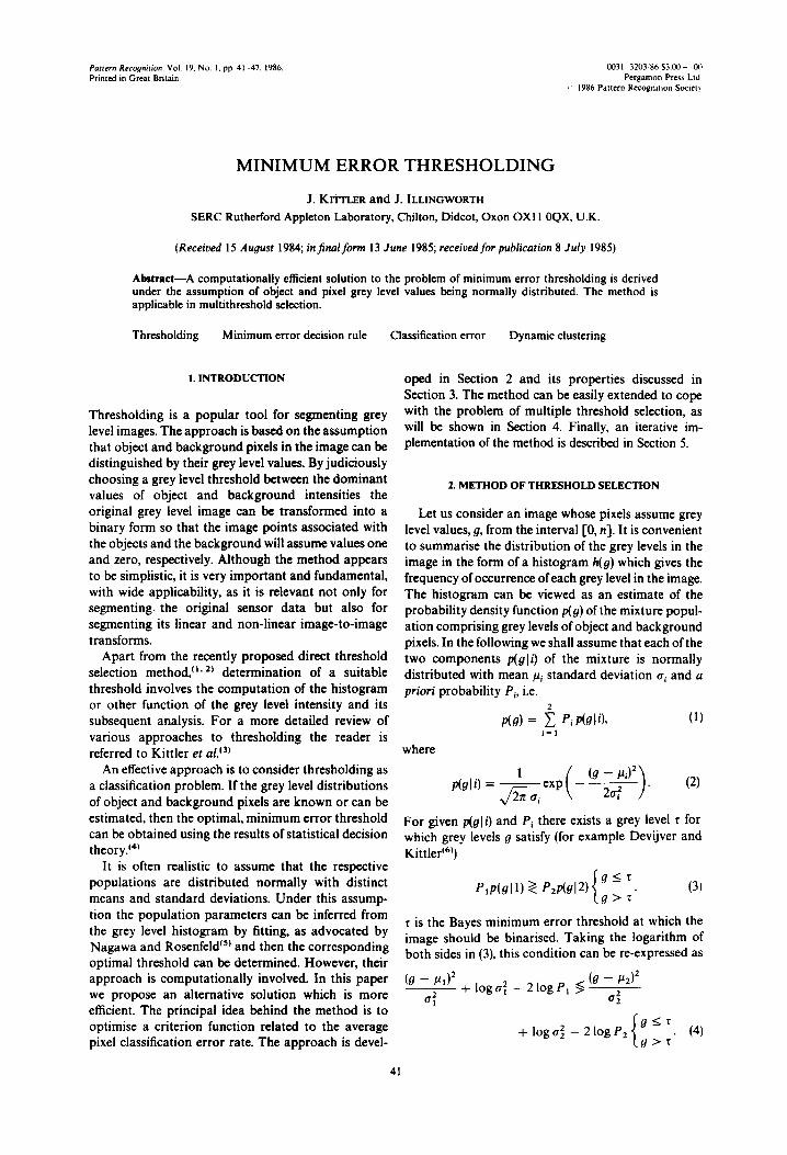
As threshold T is varied the models of the popul- ation distributions change. The better the tit between the data and the models, the smaller the overlap between the density functions and therefore the smal- ler the classification error. This behaviour is illustrated in Fig. 1 for two different values of threshold T. The corresponding overlaps of the density functions are indicated by hatching. The value of threshold T yielding the lowest value of criterion J(~, T) will give the best fit model and therefore the minimum error threshold.

In summary, instead of determining ¢ indirectly as in Nagawa and Rosenfeld, ~s) the problem of minimum error threshold selection can be formulated as one of minimising criterion J(T), i.e.

J(z) = min J(T). (13) r

It should be noted that even at the optimum value T, the models h(gli, T), i = 1, 2 will represent biased estimates of the true components of the mixture of normal probability distributions, due to the truncation of the tails of these distributions by histogram par- titioning. However, we shall assume that the effect of this bias is small and can be ignored.

Let us express criterion J(T) as

T

J(T) = ~ h(g) g=O

~,~-~ -_] + 2 log ~,(T) - 2

+ ~ h(o) g = T + l

~ j + 2 log ~(r) - 2

(14)

Substituting (5) through (7) into J(T) we find

J(T) = 1 + 2[PI(T) log trl(T ) + P2(T) log a2(T) ]

- 2 [ P I ( T ) log PI(T) + P2(T) log P2(T)]. (15)

The criterion function J(T) in (15) can be computed easily and finding its minima is a relatively simple task, as the function is smooth.

500

400

500

200

IO0

Minimum error thresholding

P,=0.5 /.L,:50 o',:15 Pz=0.5 p.z=150 o'z=15

(a)

25 50 75 I00 125 150 t75 200

43

500

400

500

200

ICO

(b)

i 25

T:50 Pj=0.25 /.L:=38 or,:9 Pz=0.75 /J.2:121 0"z:44

A

50 75 I00 125 150 175 200

5°°i (c) / ~ F ~ T:70 I ~ ' I I PI : 0 . 4 5 /~, : 4 7 ~l =1~

3 0 0 ~

200 --

~00

25 50 75 tO0 125 I~ 17'5 200

Fig. 1. (a) Grey level histogram defined by two equipopulous Gaussian distributions. Optimal threshold is at T = 100. (b, c) Population models for trial thresholds T = 50 and T = 70. Binarisation error is represented

by the hatched overlapping areas of the model population density functions.

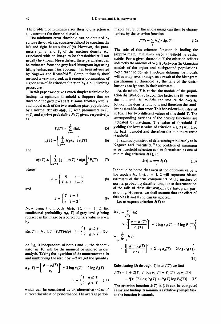
Fig. 2. Bimodal histogram. P1 = 0.5,/~l = 50, al = 4; P2 = 0.5,/t 2 = 150, a 2 = 30. Experimentally determined minimum error threshold • --- 64. Threshold selected by standard

algorithms(7 9) To = 103. Fig. 3. Criterion function J(T) for histogram of Fig. 2.

II

44 J. KITTLER and J. 1LLINGWORTH

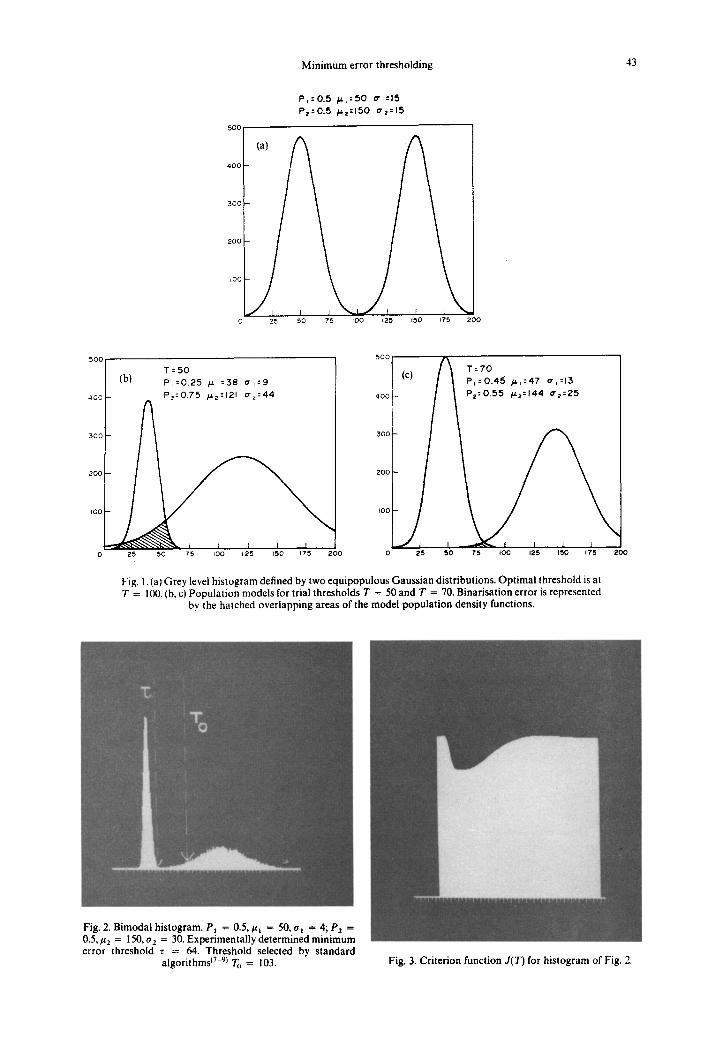
Fig.4. 50 x 50 pixel squarein a 512 × 512image. Pj = 0.99, /a 1 = 90,~r I = 10; P2 = 0.01,#2 = 170, a 2 = 10. Fig. 5. Grey level histogram of Fig. 4.

3. PROPERTIES OF THE CRITERION FUNCTION

The criterion function may have local minima at the boundaries of the interval of grey levels. However, these minima are not of interest. A unique internal minimum implies histogram bimodality and it corre- sponds to the optimum (minimum error) threshold. This has been verified experimentally on the histogram shown in Fig. 2, containing object and background grey level modes of unequal variances. Figure 3 gives the corresponding criterion function. Note that the popular threshold selection methods of Otsu fT} and Ridter, {s' ~} which use a less sophisticated model for the two modes, give a biased threshold indicated by T O in Fig. 2. The reasons why the bias occurs are discussed in Kittler and IllingworthJ 1°}

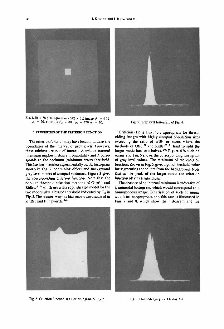
Criterion (15) is also more appropriate for thresh- olding images with highly unequal population sizes exceeding the ratio of 1:10 z or more, where the methods of Otsu ~7~ and Ridler ~8' 9~ tend to split the larger mode into two halves. "°~ Figure 4 is such an image and Fig. 5 shows the corresponding histogram of grey level values. The minimum of the criterion function, shown in Fig. 6, gives a good threshold value for segmenting the square from the background. Note that at the peak of the larger mode the criterion function attains a maximum.

The absence of an internal minimum is indicative of a unimodal histogram, which would correspond to a homogeneous image. Binarisation of such an image would be inappropriate and this case is illustrated in Figs 7 and 8, which show the histogram and the

Fig. 6. Criterion function J{T) for histogram of Fig. 5. Fig. 7. Unimodal grey level histogram.

Minimum error thresholding 45

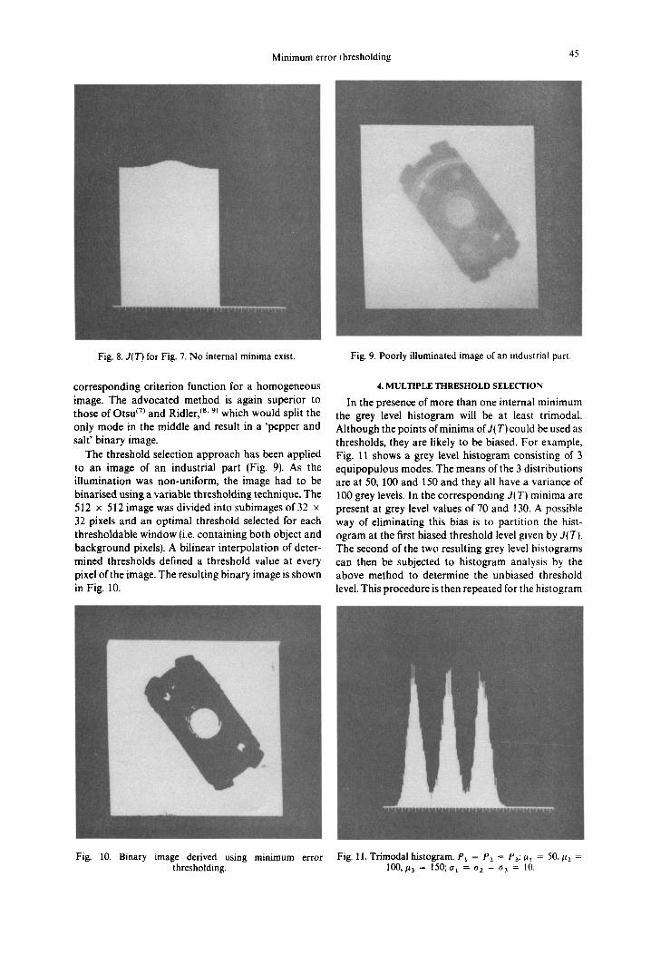
Fig. 8. J(T) for Fig. 7. No internal minima exist. Fig. 9. Poorly illuminated image of an industrial part.

corresponding criterion function for a homogeneous image. The advocated method is again superior to those of Otsu tT) and Ridler, ts' 91 which would split the only mode in the middle and result in a 'pepper and salt' binary image.

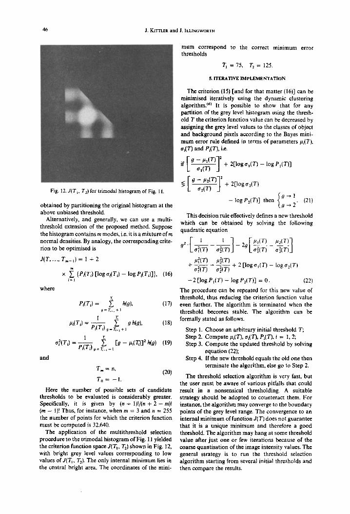
The threshold selection approach has been applied to an image of an industrial part (Fig. 9). As the illumination was non-uniform, the image had to be binarised using a variable thresholding technique. The 512 × 512 image was divided into subimages of 32 x 32 pixels and an optimal threshold selected for each thresholdable window (i.e. containing both object and background pixels). A bilinear interpolation of deter- mined thresholds defined a threshold value at every pixel of the image. The resulting binary image is shown in Fig. 10.

4. MULTIPLE THRESHOLD SELECTION

In the presence of more than one internal minimum the grey level histogram will be at least trimodal. Although the points of minima of J(T) could be used as thresholds, they are likely to be biased. For example, Fig. 11 shows a grey level histogram consisting of 3 equipopulous modes. The means of the 3 distributions are at 50, 100 and 150 and they all have a variance of 100 grey levels. In the corresponding 3(T~ minima are present at grey level values of 70 and 130. A possible way of eliminating this bias is to partition the hist- ogram at the first biased threshold level given by J(T}. The second of the two resulting grey level histograms can then be subjected to histogram analysis by the above method to determine the unbiased threshold level. This procedure is then repeated for the histogram

Fig. 10. Binary image derived using minimum error Fig. l l. Trimodalhistogram. Pt = P2 = P3,~ = 50,#2 = thresholding. 100, #3 = 150; at = a2 = 0-3 = |0.

46 J. KITTLER and J. ILLINGWORTH

r i

~i~ O ~

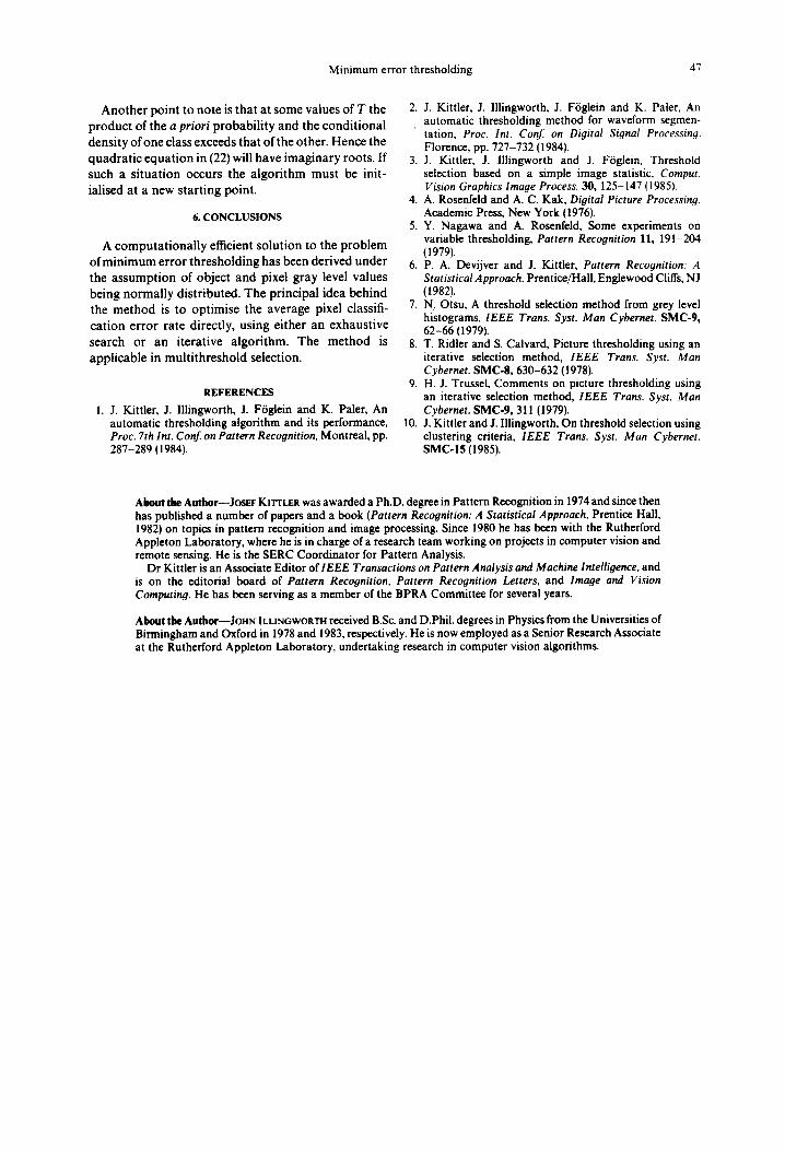
Fig. 12. J(T~, T2) for trimodal histogram of Fig. 11.

obtained by partitioning the original histogram at the above unbiased threshold.

Alternatively, and generally, we can use a multi- threshold extension of the proposed method. Suppose the histogram contains m modes, i.e. it is a mixture ofm normal densities. By analogy, the corresponding crite- rion to be optimised is

J(T ..... T=_I) = 1 + 2

x ~, {P,(T 3 [log tT,(T 3 - log P,(T,)]}, (16) i=1

where

and

r, P,.(T,) = ~ h(g), (17)

g = T , - l + 1

I r, /~,(T,) = p,(T-----~o ~ gh(o), (18)

= Z - 1 + )

1 T, a2(T3 = P,(Ti-----) ~ [g - #,(T~)] 2 h(g) (19)

g=T~_,+l

T= - - - n, (20)

To = - 1 .

Here the number of possible sets of candidate thresholds to be evaluated is considerably greater. Specifically, it is given by (n + 1)!/(n + 2 - m)! (m - I)! Thus, for instance, when m = 3 and n = 255 the number of points for which the criterion function must be computed is 32,640.

The application of the multithreshold selection procedure to the trimodal histogram of Fig. 11 yielded the criterion function space J(Tt, T2) shown in Fig. 12, with bright grey level values corresponding to low values of J(T 1, T2). The only internal minimum lies in the central bright area. The coordinates of the mini-

mum correspond to the correct minimum error thresholds

T t =75, T2= 125.

S. I T E R A T I V E I M P L E M E N T A T I O N

The criterion (15) [and for that matter (16)] can be minimised iteratively using the dynamic clustering algorithm, tr) It is possible to show that for any partition of the grey level histogram using the thresh- old T the criterion function value can be decreased by assigning the grey level values to the classes of object and background pixels according to the Bayes mini- mum error rule defined in terms of parameters/~i(T), ~r,{T) and PI(T), i.e.

if [ g - PI(T)] 2 at-~- ~ -j + 2 [ l o g a t ( T ) - logPl(T)]

>< [ e - pz(T)] z + 2[loga2(T)

- log P2(T)] then (21) " - * 2 "

This decision rule effectively defines a new threshold which can be obtained by solving the following quadratic equation

g 2 . [ 1 1 1 [ - p l ( T ) , u 2 ( T ) 7 ,~(T) .~(T) - 2 g L ~ a~(T)J

/12(T) /12(T) q try(T) a~(T) + 2 [log tr,(T) - log tr2(T)

- 2 ['log PI(T) -- log P2(T)] = 0. (22)

The procedure can be repeated for this new value of threshold, thus reducing the criterion function value even further. The algorithm is terminated when the threshold becomes stable. The algorithm can be formally stated as follows.

Step I. Choose an arbitrary initial threshold T; Step 2. Compute IA.(T), tr,,(T), Pi(T), i = 1, 2; Step 3. Compute the updated threshold by solving

equation (22); Step 4. If the new threshold equals the old one then

terminate the algorithm, else go to Step 2.

The threshold selection algorithm is very fast, but the user must be aware of various pitfalls that could result in a nonsensical thresholding. A suitable strategy should be adopted to counteract them. For instance, the algorithm may converge to the boundary points of the grey level range. The convergence to an internal minimum of function J(T) does not guarantee that it is a unique minimum and therefore a good threshold. The algorithm may hang at some threshold value after just one or few iterations because of the coarse quantisation of the image intensity values. The general strategy is to run the threshold selection algorithm starting from several initial thresholds and then compare the results.

Minimum error thresholding 47

Another point to note is that at some values of T the product of the a priori probabili ty and the conditional density of one class exceeds that of the other. Hence the quadratic equation in (22) will have imaginary roots. If such a situation occurs the algori thm must be init- ialised at a new starting point.

6. CONCLUSIONS

A computat ional ly efficient solution to the problem of minimum error thresholding has been derived under the assumption of object and pixel gray level values being normally distributed. The principal idea behind the method is to optimise the average pixel classifi- cation error rate directly, using either an exhaustive search or an iterative algorithm. The method is applicable in multi threshold selection.

REFERENCES

1. J. Kittler, J. Illingworth, J. F6glein and K. Paler, An automatic thresholding algorithm and its performance, Proc. 7th Int. Conf. on Pattern Recognition, Montreal, pp. 287-289 (1984).

2. J. Kittler, J. Illingworth, J. F6glein and K. Paler, An automatic thresholding method for waveform segmen- tation, Proc. Int. Conf. on Digital Signal Processing. Florence, pp. 727-732 (1984).

3. J. Kittler, J. Illingworth and J. F6glein, Threshold selection based on a simple image statistic, Comput. Vision Graphics Image Process. 30, 125-147 (1985).

4. A. Rosenfeid and A. C. Kak, Digital Picture Processing. Academic Press, New York (1976).

5. Y. Nagawa and A. Rosenfeld, Some experiments on variable thresholding, Pattern Recognition 11, 191-204 (1979).

6. P. A. Devijver and J. Kittler, Pattern Recognition: A Statistical Approach. Prentice/Hall, Englewood Cliffs, NJ (1982).

7. N, Otsu, A threshold selection method from grey level histograms, IEEE Trans. Syst. Man Cybernet. SMC-9, 62-66 (1979).

8. T. Ridler and S. Calvard, Picture thresholding using an iterative selection method, IEEE Trans. Syst. Man Cybernet. SMC-8, 630-632 (1978).

9. H. J. Trussel, Comments on picture thresholding using an iterative selection method, IEEE Trans. Syst. Man Cybernet. SMC-9, 311 (1979).

10. J. Kittler and J. Illingworth, On threshold selection using clustering criteria, IEEE Trans. Syst. Man Cybernet. SMC-15 (1985).

About the Autbor--Josar KtTrLER was awarded a Ph.D. degree in Pattern Recognition in 1974 and since then has published a number of papers and a book (Pattern Recognition: A Statistical Approach, Prentice Hall, 1982) on topics in pattern recognition and image processing. Since 1980 he has been with the Rutherford Appleton Laboratory, where he is in charge of a research team working on projects in computer vision and remote sensing. He is the SERC Coordinator for Pattern Analysis.

Dr Kittler is an Associate Editor of l EEE Transactions on Pattern Analysis and Machine Intelligence, and is on the editorial board of Pattern Recognition, Pattern Recognition Letters, and Image and Vision Computing. He has been serving as a member of the BPRA Committee for several years.

About the Author--JoHN ILLINGWORTH received B.Sc. and D.Phil. degrees in Physics from the Universities of Birmingham and Oxford in 1978 and 1983, respectively. He is now employed as a Senior Research Associate at the Rutherford Appleton Laboratory, undertaking research in computer vision algorithms.