minimum hot surface ignition temperature diagnostics
TRANSCRIPT

Purdue University Purdue University
Purdue e-Pubs Purdue e-Pubs
Open Access Theses Theses and Dissertations
January 2015
Minimum Hot Surface Ignition Temperature Diagnostics Including Minimum Hot Surface Ignition Temperature Diagnostics Including
Infrared Imagery Infrared Imagery
Jesse Filmore Adams Purdue University
Follow this and additional works at: https://docs.lib.purdue.edu/open_access_theses
Recommended Citation Recommended Citation Adams, Jesse Filmore, "Minimum Hot Surface Ignition Temperature Diagnostics Including Infrared Imagery" (2015). Open Access Theses. 1043. https://docs.lib.purdue.edu/open_access_theses/1043
This document has been made available through Purdue e-Pubs, a service of the Purdue University Libraries. Please contact [email protected] for additional information.


MINIMUM HOT SURFACE IGNITION TEMPERATURE DIAGNOSTICS INCLUDING INFRARED IMAGERY
A Thesis
Submitted to the Faculty
of
Purdue University
by
Jesse F. Adams
In Partial Fulfillment of the
Requirements for the Degree
of
Master of Science in Aeronautics and Astronautics
December 2015
Purdue University
West Lafayette, Indiana

ii
To my Mother and Father,

iii
ACKNOWLEDGEMENTS
In many ways, this document is the culmination of my time and experiences at
Purdue. It is the byproduct of not only my own effort, but of the help and guidance many
others have given me on the way. I must begin by thanking my advisor, Professor Jay
Gore for both providing me this tremendous opportunity and for his patience. I am also
duly grateful to Professor Stephen Heister and Professor Timothée Poupoint for serving
on my thesis committee.
I must also express my gratitude to several fellow students at working at Maurice J.
Zucrow Laboratories. Acknowledgements go to Steven Hunt, Heather Wiest, Rohan
Gejii, Vikrant Goyal, Andrei Anghelus, and Luke Mishler for all of their assistance in
helping me realize this project. More than just outstanding engineers, they are all also
outstanding people.
Sincere thanks go to Chris Potter and Charles Sese for their support and friendship
throughout this process, and for always having a pep talk ready when I was unsure if I
would make it.

iv
Lastly, a very special thank you to Scott Meyer. I would never have accomplished
this level of work without his advice and guidance. I am truly a better engineer from
having known him.
This project was supported by Rolls-Royce Corporation through their UTC
collaboration with Purdue University.

v
TABLE OF CONTENTS
Page
LIST OF FIGURES .......................................................................................................... vii
LIST OF TABLES ............................................................................................................. xi
NOMENCLATURE .......................................................................................................... iii
ABSTRACT ...................................................................................................................... xv
CHAPTER 1. MOTIVATION AND OBJECTIVES ......................................................... 1
1.1 Motivation ................................................................................................................. 1
1.2 Objectives .................................................................................................................. 4
CHAPTER 2. LITERATURE REVIEW ............................................................................ 6
2.1 Fundamentals of Hot Surface Ignition ...................................................................... 6
2.2 Quiescent Hot Surface Experiments ......................................................................... 9
2.3 Previous Hot Surface Ignition Experiments in a Crossflow ................................... 13
2.4 The Wright-Patterson Test Rig ............................................................................... 16
CHAPTER 3. THE DESIGN PROCESS.......................................................................... 22
3.1 Design Rational ....................................................................................................... 22
3.2 Dimensioning the Experimental Rig ....................................................................... 26
3.3 Hot Centerbody Design ........................................................................................... 31
3.4 Ceramic Materials ................................................................................................... 45
3.5 Supporting the Hot Centerbody............................................................................... 52
3.6 Flow Conditioning .................................................................................................. 57
3.7 Window Assembly .................................................................................................. 74
3.8 Injection ................................................................................................................... 80
3.9 Support Stand .......................................................................................................... 90

vi
Page
3.10 Instrumentation and Sensory Equipment .............................................................. 97
3.11 Provisions for Complicating Flow Features ........................................................ 100
3.12 Pressure and Temperature Rake .......................................................................... 102
CHAPTER 4. PRELIMINARY TESTS ......................................................................... 103
4.1 Flat Plate Test Article Experiments ...................................................................... 103
4.2 Simple Cylinder Tests ........................................................................................... 116
CHAPTER 5. VALIDATING THE RIG ........................................................................ 123
5.1 Initial Test with Propane ....................................................................................... 123
5.2 Initial Tests with JP-8 ............................................................................................ 125
CHAPTER 6. CONCLUSIONS AND FUTURE WORK .............................................. 133
LIST OF REFERENCES ................................................................................................ 134
APPENDICES
A.1 MATLAB Script for Droplet Trajectory Analysis ............................................... 138
A.2 Suggested Flow Metering Tables ......................................................................... 142
A.3 Plumbing and Instrumentation Diagram .............................................................. 147
A.4 Engineering Drawings .......................................................................................... 148

vii
LIST OF FIGURES
Figure Page
Figure 1.1 Damaged engine No. 2 of Qantas Flight 32 [4]................................................. 2 Figure 1.2. AE 3007 divided into 25 zones for the heat rejection model [6] ...................... 3 Figure 1.3. Skin temperatures compared against database MHSIT for JP-8/Jet-A [6] ....... 4 Figure 2.1. Flammability/ignition regimes as function of temperature and fuel vapor pressure [8].......................................................................................................................... 8 Figure 2.2. Heat transfer and mass transfer paths for the spherical droplet model [12] ..... 9 Figure 2.3. Test stand for an isothermal plate [8] ............................................................. 11 Figure 2.4. Ignition probability as a function of plate temperature for aviation fluids [8] 12 Figure 2.5. Experimental rig used by Graves [15] ............................................................ 13 Figure 2.6. Cut side view of Myronuk test apparatus [14] ............................................... 15 Figure 2.7. The Wright-Patterson test article, the AENFTS [5] ....................................... 16 Figure 2.8. Close-up of test section with connection to bleed air source and flow direction shown ................................................................................................................................ 17 Figure 2.9. Bleed air ducting that comprised much of the High Realism article, thermocouple locations are boxed in red [5] ..................................................................... 19 Figure 3.1. Wright-Patterson heating methods for the Simple Duct test article [5] ......... 23 Figure 3.2. Wright-Patterson test article in vertical (right) and horizontal (left) orientations [5] .................................................................................................................. 24 Figure 3.3. Circle Inscribed inside Octagon ................................................................. 27 Figure 3.4. 8 congruent interior triangles………………………………………………….....27
Figure 3.5. Octagonal Duct with Rectangular Window Holes and Attachment Flange at the base.............................................................................................................................. 30 Figure 3.6. Center Cylinder .............................................................................................. 30 Figure 3.7. The Inconel Hot Centerbody with excavated center diameter and heater holes........................................................................................................................................... 38 Figure 3.8. The arc length between heaters is shown in yellow with radial distances in blue .................................................................................................................................... 40 Figure 3.9. A .125 inch thermocouple probe clearance hole between 2 heater holes ....... 42 Figure 3.10. Axial location of thermocouple sensing points ............................................ 43

viii
Figure Page Figure 3.11. Thermocouple profile probe with sensing points identified ......................... 44 Figure 3.12. Zone configuration in the Hot Centerbody ................................................... 44 Figure 3.13. Cartridge Heater with insulating beads shown ............................................. 45 Figure 3.14. Macor® Ceramic End after machining ........................................................ 47 Figure 3.15. Grade ‘A’ lava Ceramic Sleeve after machining .......................................... 47 Figure 3.16.Ssemi-infinite solid model for the interface between solid A and solid B .... 49 Figure 3.17. Cantilever Base Plate prior to welding ......................................................... 53 Figure 3.18. The bare Cantilevered Support and Cantilever Base Plate post welding ..... 54 Figure 3.19. End Piece with 3.5 inch diameter lip, and .5 inch rod clearance hole on the far face .............................................................................................................................. 55 Figure 3.20. The bare Cantilevered Support at the proper (horizontal) orientation ......... 56 Figure 3.21. Cantilevered Support with the Ceramic Sleeve ............................................ 56 Figure 3.22. After adding first Ceramic End .................................................................... 56 Figure 3.23. With Hot Centerbody and 2nd Ceramic End in place ................................... 57 Figure 3.24. With the End Piece secured (the Belleville washer and nut are visible) ...... 57 Figure 3.25. The stainless steel 304 Base component ...................................................... 61 Figure 3.26. The annular Plenum Vessel with red arrows depicting air flow .................. 62 Figure 3.27. Plenum Vessel prior to welding with 1” diameter flow entrances visible ... 63 Figure 3.28. The Orifice Plate prior to welding ................................................................ 65 Figure 3.29. Effect of the ratio of plate thickness to hole diameter at Re=2000 on Cd [24]........................................................................................................................................... 67 Figure 3.30. Effect of the ratio of hole diameter to hole pitch on Cd [24] ........................ 68 Figure 3.31. The Orifice Plate, Plenum Vessel, Center Cylinder and Base post welding 69 Figure 3.32. The 300 pound, 2 inch weld-neck flange prior to welding........................... 70 Figure 3.33. Pipe fittings prior to welding (pipe lengths are not shown) ......................... 70 Figure 3.34. The 90° elbow and 1.5 to 1 inch reducer ...................................................... 71 Figure 3.35. Welded plumbing to plenum connection ...................................................... 71 Figure 3.36. The permanent plumbing assembly after welding ........................................ 72 Figure 3.37. First elbowed pipe section connected to the permanent assembly ............... 73 Figure 3.38. Second elbowed section with 2 inch flanges on either end .......................... 73 Figure 3.39. Braided stainless steel flexline ..................................................................... 74 Figure 3.40. Transmission curve for sapphire [25] ........................................................... 75 Figure 3.41. Transmission curves for various grades of fused silica [26] ........................ 76 Figure 3.42. Window Flanges with clearance hole detail ................................................. 77 Figure 3.43. Fused silica window before being placed inside a window flange .............. 78 Figure 3.44. The installed fused silica windows and window flanges .............................. 78 Figure 3.45. Cracked windows from initial thermal cycling ............................................ 79 Figure 3.46. Grafoil® gaskets used to protect and seal window assemblies .................... 80 Figure 3.47. Top view of liquid drop injection into a gaseous cross-flow ....................... 83 Figure 3.48. Droplet Trajectory for the Left Side of an 80° Spray Fan ............................ 85

ix
Figure Page Figure 3.49. Droplet Trajectory for the Right Side of an 80° Spray Fan .......................... 85 Figure 3.50. Aluminum Valve Panel prior to pluming and mounting .............................. 87 Figure 3.51. Fuel Filter procured from Norman Filter Company ..................................... 88 Figure 3.52. Sample check valve ...................................................................................... 89 Figure 3.53. Manual ball valve used to relieve vessel pressure ........................................ 89 Figure 3.54. Relief valve ................................................................................................... 90 Figure 3.55. Test support stand prior to being bolted to the test facility floor ................. 91 Figure 3.56. Welded Base component with fastener thru-holes along the edges ............. 92 Figure 3.57. Electrical box secured by uni-strut pieces to the back of the HSIC test rig . 95 Figure 3.58. Assembled HSIC test rig without Octagonal Duct ....................................... 95 Figure 3.59. Assembled HSIC rig with Octagonal Duct and Window Assemblies ......... 96 Figure 3.60. Assembled HSIC rig during cartridge heater test at 1400°F (760°C) set point........................................................................................................................................... 96 Figure 3.61. Thermocouple installed atop Plenum Vessel via welded port...................... 98 Figure 3.62. Pressure transducer ported and mounted to the Plenum Vessel ................... 99 Figure 3.63. The high speed infrared camera ................................................................. 100 Figure 3.64. The plugged holes for flow features ........................................................... 101 Figure 3.65. Proposed design for the pressure-temperature rake.................................... 102 Figure 4.1. The complete experimental arrangement for the flat plate tests ................... 104 Figure 4.2. Copper plate with installed cartridge heaters and bolt holes for the steel plate......................................................................................................................................... 105 Figure 4.3. Copper and stainless steel plates together with electrical leads ................... 105 Figure 4.4. Syringe pump................................................................................................ 106 Figure 4.5. JP-8 ignition at 737±2°C and 100% ignition probability ............................. 108 Figure 4.6. MIL-PRF-5606 ignition at 721±2°C and 100% ignition probability ........... 108 Figure 4.7. Ignition probability curve for JP-8 ............................................................... 110 Figure 4.8. Ignition probability curve for MIL-PRF-5606 ............................................. 111 Figure 4.9. Instantaneous image of JP-8 ignition at 810°C set point for 2.58±.03µm ... 112 Figure 4.10. Instantaneous image of MIL-PRF-5606 ignition at 780°C set point for 2.58±.03µm ..................................................................................................................... 113 Figure 4.11. JP-8 at t = 0 secs, ignition starts ................................................................. 115 Figure 4.12. JP-8 at t = 100ms, initial flame rise ............................................................ 115 Figure 4.13. JP-8 at t = 200ms, flame peak .................................................................... 115 Figure 4.14. JP-8 at t = 300ms, flame diminishing prior to extinction ........................... 116 Figure 4.15. Cylindrical test article atop porous ceramic block and ceramic fiber bedding......................................................................................................................................... 117 Figure 4.16. Cylindrical test article at a 650°C set point ................................................ 117 Figure 4.17. Cylindrical test article at a 1000°C set point .............................................. 118 Figure 4.18. JP-8 on the cylinder at t = 0s, ignition starts .............................................. 119 Figure 4.19. JP-8 on the cylinder at t = 110ms, flame propagates along cylinder length119

x
Figure Page Figure 4.20. JP-8 on the cylinder at t = 220ms, flame catches on the ceramic wool ...... 120 Figure 4.21. JP-8 on the cylinder at t = 330ms, flame is prolonged by stabilization on the wool................................................................................................................................. 120 Figure 4.22. Ignition probability curve for JP-8 on the cylindrical test article ............... 121 Figure 5.1 Test article heated to 843±3°C with spray nozzle visible ............................. 126 Figure 5.2 JP-8 ignition for 816±3°C at 106±15°C air temperature and .37±.03 m/s air velocity ............................................................................................................................ 127 Figure 5.3 Effect of air velocity on MHSIT of JP-8 at 149°C air temperature............... 131

xi
LIST OF TABLES
Table Page Table 2.1. Effect of Duct Conditions on Minimum Hot Surface Ignition Temperature (MHSIT) ........................................................................................................................... 20 Table 3.1. Dimensions of Scaled Test Sections ................................................................ 27 Table 3.2. Representative Air Mass Flowrates ................................................................. 28 Table 3.3. Material properties of Inconel 718 and ceramic components .......................... 50 Table 3.4. Representative Air Heating Rates .................................................................... 58 Table 3.5. Air Plenum Conditions at 70°F ........................................................................ 63 Table 3.6. Initial Scaled Fuel Flowrates for HSIC Rig ..................................................... 81 Table 3.7. Masses for the Various HSIC rig parts ............................................................ 93 Table 4.1. Ignition Data for JP-8 .................................................................................... 109 Table 4.2. Ignition Data for MIL-PRF-5606 .................................................................. 110 Table 4.3. Ignition Data for JP-8 on the cylindrical test article ...................................... 120 Table 5.1 Propane Test Matrix, October 30, 2015 .......................................................... 124 Table 5.2 JP-8 Test Matrix, October 31, 2015 ................................................................ 126 Table 5.3 JP-8 Test Matrix, December 14, 2015 ............................................................ 129

xii
NOMENCLATURE
Symbols Description
𝑊𝑊 Molar rate per unit volume
𝑍𝑍 Pre-exponential factor
𝑐𝑐 Reactant concentration
𝐸𝐸𝑎𝑎 Activation Energy
R Universal Gas Constant
T Temperature
𝑄𝑄 Heat rate
𝑉𝑉 Volume
∆𝐻𝐻𝑟𝑟° Heat of reaction per mole
ℎ Generalized heat transfer coefficient
𝐴𝐴 Area
𝜌𝜌 Density
𝑐𝑐𝑝𝑝 Specific Heat
𝑡𝑡 Time
𝑘𝑘 Generalized thermal conductivity
𝜆𝜆 Latent heat of vaporization
𝑎𝑎 Side length of a geometric object
𝜃𝜃 Angle
𝑈𝑈,𝑢𝑢 Velocity
�̇�𝐸 Generalized energy rate
ℎ� Average convective heat transfer coefficient
𝑣𝑣 Kinematic viscosity

xiii
𝑅𝑅𝑅𝑅 Reynolds number
𝐿𝐿, 𝑙𝑙, 𝑥𝑥 Length scale
𝑁𝑁𝑢𝑢���� Nusselt Number
𝑃𝑃𝑃𝑃 Prandtl number
𝜀𝜀 Emissivity
𝜎𝜎 Stefan-Boltzmann’s constant
𝛼𝛼 Absorptivity
𝐺𝐺 Total incident radiation
𝐵𝐵𝐵𝐵 Biot number
𝑆𝑆 Arc length
𝑃𝑃 Radius
𝛼𝛼𝑒𝑒𝑒𝑒𝑝𝑝 Linear coefficient of thermal expansion
𝑞𝑞" Heat flux
𝛿𝛿𝑝𝑝 Thermal penetration depth
�̇�𝑚 Mass flow rate
𝐶𝐶𝑑𝑑 Fluid discharge coefficient
𝛾𝛾 Ratio of specific heats
𝑝𝑝 Pressure
𝑀𝑀 Total mass
𝑃𝑃 Probability
𝑏𝑏𝑜𝑜 ,𝑏𝑏1 Coefficients for logistic curve fit
𝐷𝐷𝑎𝑎 Damköhler number
∆ Delta, signifying a change in state

xiv
Subscripts Description
𝑐𝑐ℎ𝑅𝑅𝑚𝑚 Relating to chemical process
𝑠𝑠𝑢𝑢𝑃𝑃𝑃𝑃 Relating to system surroundings
𝑐𝑐𝑐𝑐𝑐𝑐𝑐𝑐 Relating to conduction
𝑅𝑅𝑎𝑎𝑐𝑐 Relating to radiation heat transfer
𝑠𝑠𝑡𝑡 Relating to energy storage
𝐵𝐵𝑐𝑐 Relating to energy inflow
𝑐𝑐𝑢𝑢𝑡𝑡 Relating to energy outflow
𝑔𝑔𝑅𝑅𝑐𝑐 Relating to energy generation
𝑠𝑠,𝑤𝑤 Relating to a surface or wall
∞ Freestream condition
𝑓𝑓 Relating to a fluid as opposed to a solid
𝐿𝐿 Relating to a length scale or displacement
𝑐𝑐 Indicates characteristic dimension
𝐵𝐵 Relating to an initial condition
𝑡𝑡 Relating to a throat restriction
1 Relating to an upstream condition
𝑔𝑔 Relating to a gas
𝑙𝑙 Relating to a liquid
𝑥𝑥 Specifically relating to x displacement
𝑦𝑦 Specifically relating to y displacement
𝑐𝑐𝑚𝑚 Indicating center of mass
Abbreviations Description
AENFTS Aircraft Engine Nacelle Fire Test Simulator
AFRL Air Force Research Laboratory
MHSIT Minimum Hot Surface Ignition Temperature
HSIC Hot Surface Ignition in Crossflow
ABSTRACT
Adams, Jesse, F. M.S., Purdue University, December 2015. Minimum Hot Surface Ignition Temperature Diagnostics Including Infrared Imagery. Major Professor: Jay P. Gore, School of Aeronautical and Astronautical Engineering
Hot surface ignition caused by a leak from ruptured fuel or hydraulic lines impinging
on high temperature engine surfaces poses dangers to both the automotive and aviation
industries. Many previous studies have investigated the aircraft engine nacelle
environments most conducive to hot surface ignition, but alterations and improvements in
turbofan engine design have left many of these studies obsolete or in need of expansion.
A literature review is presented to survey these previous studies. Particular emphasis
is made on a study conducted under the Air Force Wright Aeronautical Laboratory at
Wright-Patterson Air Force Base. Additionally, a distinction is made between hot surface
ignition and auto-ignition.
Finally, the design and verification of a new experimental apparatus to investigate hot
surface ignition for modern turbofan engines is presented. Supplementary experiments
including infrared imaging on a quiescent hot surface are also described.
xvi

CHAPTER 1. MOTIVATION AND OBJECTIVES
1.1 Motivation The threat of hot surface ignition and its underlying causes are a source of ongoing
concern for the aircraft and automotive industries. Property losses attributable to motor
vehicle fires total in excess of 1 billion dollars annually in the U.S. alone [1]. Moreover,
at least two-thirds of these fires can be traced back to vehicle engine compartments [1],
where hot manifold surfaces and numerous fuel lines often exist in close proximity to one
another. Dramatic reminders of the dangers of hot surface ignition in aircraft are found in
both recent and not so recent headlines. The explosion of Trans World Airlines Flight
800 in July of 1996 was a fatal and costly disaster that resulted in the loss of 230 lives
[2]. It was concluded during the subsequent investigation that the explosion was the result
of a flammable mixture of fuel and air inside the aircraft’s center wing fuel tank being
subject to tremendous heat transfer rates due to the tanks contact with the surface of the
hot, air conditioning packs located directly below [2]. In November 2010, Qantas Flight
32 was forced to make an emergency landing when a ruptured lubricant line led to an oil
fire in one of the aircraft’s Rolls-Royce Trent 900 engines [3].
1

Figure 1.1 Damaged engine No. 2 of Qantas Flight 32 [4]
Rolls-Royce’s sponsorship of the present research is motivated by a desire to verify
and extend the database it currently uses to certify the safety of its engines against the
danger of hot surface ignition. The database was originally established from experimental
trials conducted by Johnson et al. [5] at Wright-Patterson Air Force Research Lab. When
evaluating the minimum hot surface ignition temperature of an aircraft fluid, Rolls-Royce
applies a heat rejection model to predict engine skin temperature [6]. The heat rejection
model subdivides the engine into cylindrical zones of interests, and calculates a single
expected skin temperature for each zone. The average zone length is between 4 and 5
inches. The model incorporates one dimensional conduction through the core engine
casing as well as the inner and outer bleed air ducts [6]. The effects of conduction
propagate across zones, but radiation and convection are specifically treated for the
cylindrical control volume of a single zone.
2

Figure 1.2. AE 3007 divided into 25 zones for the heat rejection model [6]
The skin temperature predicted for a zone is compared against the hot surface ignition
database to produce what is referred to as a minimum hot surface ignition temperature or
MHSIT margin [6]. The margin is the predicted skin temperature subtracted from the
database temperature. Positive margins are associated with engine safety. The ignition
temperature referenced from the database considers multiple factors including: leak fluid,
local air temperature, local air velocity, pressure, and leak type (spray or stream).
3

Figure 1.3. Skin temperatures compared against database MHSIT for JP-8/Jet-A [6]
Despite its usefulness, the current database presents a number of frustrations for Rolls-
Royce. In the database, air velocities never exceed 11 ft/s. This is almost a full order of
magnitude lower than velocities observed inside the engine nacelle. The database
contains data that was taken over 2 decades ago. Some fluids that appear in the database,
such as JP-4, have been phased out of general use while modern aircraft fluids such as the
MIL-PRF-23699, a new lubricating oil, do not appear at all. The hot surface ignition
project at Purdue is intended to redress these issues.
1.2 Objectives At the outset of the hot surface ignition project, the following objectives were
enumerated:
1. Conduct a literature review
a. To cleanly identify the distinction between auto-ignition and hot surface
ignition phenomena.
4

b. To survey the range of hot surface ignition studies previously conducted
c. To identify and to describe in detail the old experimental apparatus used to
create the existing hot surface ignition database
2. Design and construct an experimental rig that is scaled, modular, and expands the
scope of achievable experimental conditions from those already in the minimum
hot surface ignition temperature database.
3. Begin the process of verifying the experimental rig’s operation by repeating
selected test conditions from the established database.
5

CHAPTER 2. LITERATURE REVIEW
2.1 Fundamentals of Hot Surface Ignition Throughout the course of the literature review, multiple sources stressed the inherent
differences between auto-ignition and hot surface ignition [7-9]. Thermal ignition is
broadly understood to be the result of a combustible mixture (either with or without an
external heating source) undergoing an exothermic reaction such that the heat release
from reaction overcomes the heat losses to the surrounding environment [10]. This is
modeled in theories by both Semenov [10] and Frank-Kamenetskii [10]. Semenov
applied his approach to a gas mixture and assumed the rate of chemical reaction adheres
to the Arrhenius law, with W representing a molar rate per unit volume.
𝑊𝑊 = 𝑍𝑍𝑐𝑐𝑛𝑛𝑅𝑅−𝐸𝐸𝑎𝑎
𝑅𝑅𝑅𝑅� [Eq. 2-1]
In equation 2-1, Z is the pre-exponential factor, c is the initial reactant concentration, Ea is
the activation energy, R is the universal gas constant, and T is the temperature of the
system. The heating rate from chemical reaction was thus:
𝑄𝑄𝑐𝑐ℎ𝑒𝑒𝑒𝑒 = 𝑉𝑉∆𝐻𝐻𝑟𝑟°𝑍𝑍𝑐𝑐𝑛𝑛𝑅𝑅−𝐸𝐸𝑎𝑎
𝑅𝑅𝑅𝑅� [Eq. 2-2]
The heat of reaction per mole is ∆𝐻𝐻𝑟𝑟° and V is the total system volume. Semenov modeled
the heat loss to the surroundings [10] in the general formal of Newton’s law of cooling.
𝑄𝑄𝑠𝑠𝑠𝑠𝑟𝑟𝑟𝑟 = ℎ(𝑇𝑇 − 𝑇𝑇𝑤𝑤)𝐴𝐴 [Eq. 2-3]
6

The temperature of the system is given as T, the temperature of the system walls is Tw, A
is the surface area of the system wall, and h is a generalized heat transfer coefficient. The
critical condition that sits on the boundary between ignition and extinction is the point
when equations 2-2 and 2-3 are set equal to one another. Semenov effectively models the
system as a well-stirred reactor at a uniform temperature [10]. Incidentally, these
conditions align with those for auto-ignition. Frank-Kamenetskii presents a more rigorous
formulation that takes into account temperature non-uniformity within the reacting system
[10].
𝜌𝜌𝑐𝑐𝑝𝑝𝜕𝜕𝑅𝑅𝜕𝜕𝜕𝜕
= 𝜌𝜌∆𝐻𝐻𝑟𝑟°𝑍𝑍𝑅𝑅−𝐸𝐸𝑎𝑎
𝑅𝑅𝑅𝑅� + 𝑘𝑘∇2𝑇𝑇 [Eq.2-4]
The left-hand expression is the heating rate for the system. The first term on the right is the
heating rate from chemical release, and the final expression is of the conduction heat loss
at the system boundaries [10]. To an extent, the differences in Semenov’s and Frank-
Kamenetskii’s approaches to ignition theory parallels the differences between auto-ignition
and hot surface ignition. The auto-ignition temperature of a flammable fluid is determined
under a well-documented standard, ASTM E659 [11]. To find auto-ignition temperature, a
carefully metered sample of flammable liquid is inserted into a uniformly heated, 500 mL
glass flask at ambient pressure. The temperature is steadily raised until the ignition is
observed. There is no such standardization for hot surface ignition, which is most
frequently considered within highly non-uniform environments and is subject to a host of
variables including [8]: irregular surface geometry, airflow near the surface, ambient air
temperature [5], whether fluid is introduced as a spray or stream, etc. Kuchta phrases the
difference particularly clearly in terms of the quality of the ignition source [10]. Strong
ignition sources have incredibly high heating rates and also tend to be highly localized
7

spatially or temporally (or both). Examples of this are spark ignition, lasers, and pilot
flames. A weaker form of forced ignition is seen in diesel engines which exhibit a more
uniformly distributed system energy, but must rely on compression to achieve ignition.
Weaker still is auto-ignition which has a uniform distribution of system energy, but lacks
any active compression. The weakest of all these ignition sources is the hot surface. It lacks
both the high energy density of a spark, and the well-distributed properties seen in auto-
ignition since the flammable mixture only contacts the hot surface at specific locations
within the ignition system. Accordingly, experimentally observed hot surface ignition
temperatures for flammable fluids are frequently at least 300°C higher than corresponding
auto-ignition temperatures. Colwell [8] provides an elucidating figure on the differences
across these ignition sources.
Figure 2.1. Flammability/ignition regimes as function of temperature and fuel vapor pressure [8]
8

2.2 Quiescent Hot Surface Experiments The experimental work surveyed for this research is divided into two categories:
those that did droplet ignition in quiescent environments and those that attempted to
simulate the harsher environments of aircraft engine bays complete with crossflows,
recirculation zones, and irregular surface geometries. Although the hot surface ignition
project at Purdue is firmly in the latter category, the quiescent experiments offered
considerable insight into the fundamentals of hot surface ignition.
The Leidenfrost phenomenon is intimately linked to droplet ignition on hot surfaces.
When small quantities of liquid are spilled onto a surface that well exceeds their
saturation temperature, a thin vapor film forms between the surface and the liquid.
Because the liquid drop is only in contact with the vapor, it glides smoothly across the
surface without wetting it. This vapor film has the added effect of acting as an insulator,
slowing the evaporation rate of the drop. Gottfried et al. [12] describe the heat transfer
processes attendant to the Leidenfrost effect on a spherical drop.
Figure 2.2. Heat transfer and mass transfer paths for the spherical droplet model [12]
𝑄𝑄𝑐𝑐𝑜𝑜𝑛𝑛𝑑𝑑 + 𝑄𝑄𝑅𝑅𝑎𝑎𝑑𝑑1 + 𝑄𝑄𝑅𝑅𝑎𝑎𝑑𝑑2 = 𝑊𝑊1�𝜆𝜆 + 𝑐𝑐𝑝𝑝(𝑇𝑇𝑣𝑣 − 𝑇𝑇𝑠𝑠)� + 𝑊𝑊2𝜆𝜆 [Eq. 2-5]
9

Heat is conducted to the lower surface of the droplet through the vapor film. The
overheated plate also radiates heat to the upper (Qrad2) and lower (Qrad1) surfaces. These
rates differ, however since radiation on the lower half occurs through the vapor film. Heat
is lost from the droplet through the advection that accompanies evaporation; once again,
W gives the rate. The latent heat of evaporation is represented by the symbol, λ. The
vapor transported from the lower surface is trapped inside the vapor film and raised to its
temperature. A sensible heat term is added to complete the energy balance. Numerical
methods can be applied to this balance to approximate a droplet lifetime [12].
Experiments that vary drop volume on a heated plate could then be used to identify the
effects, if any, that drop lifetime has on either hot surface ignition temperature or the
ignition delay.
A number of researchers performed experiments wherein a metered droplet of
flammable liquid was deposited on the surface of an isothermal plate [7-9, 13]. In these
researches, the flammable fluids were tested exhaustively. It was typical to conduct over
200 ignition tests per fluid [8]. These experiments were valuable for their relative
simplicity and repeatability. The apparatus used by Colwell [8] is presented as an
example in the figure below.
10

Figure 2.3. Test stand for an isothermal plate [8]
The test surface is a 48 cm by 38 cm by 4.8 cm thick stainless steel 304 plate. The 3-
sided enclosure is a draft shield to minimize any cross-flow effects. The plate is
electrically heated with a nichrome wire heating element, and the purpose of the
insulation is to keep the plate temperature relatively isothermal. Tests were conducted
with a wide variety of both automotive and aviation fluids. Rather than observing a
specific plate temperature at which the fuel suddenly ignited (as with the auto-ignition
temperature), ignition was found to be probabilistic in nature. At an established plate
temperature, ignition was best characterized through a probability curve with the onset
occurring at some minimum plate temperature. Ignition probability subsequently rose
with increasing temperature across a range of plate settings before reaching the point
when the probability of ignition became 100%. Colwell’s [8] findings for several aviation
fluids are shared in the plot below. Data was plotted using a logistic regression curve.
The focus on the results for the aviation fluids came from the large overlap with the fluids
11

that were eventually selected for experimentation on the Purdue hot surface ignition
project.
Figure 2.4. Ignition probability as a function of plate temperature for aviation fluids [8]
Probabilistic ignition behaviors were reported for practically all the quiescent plate
experiments reviewed. This behavior was not reported for any of the higher velocity,
higher realism test articles described in the upcoming section. This omission is either due
to no attempt being made to quantify an ignition probability or because probabilistic
ignition no longer applies. On these complex test articles, fuel is not administered as a
drop, but as a stream or spray or steady drip. Odd surface geometries and bypass air
streams add greater barriers to ignition. If this probabilistic behavior no longer applies, it
could be a byproduct of these barriers rendering ignition much less likely to occur. Future
work might focus on applying these probabilistic curves to more complex test
environments.
12

2.3 Previous Hot Surface Ignition Experiments in a Crossflow This section summarizes the experimental work on hot surface ignition done by
Myronuk [14], Graves [15], and Ingerson [16]. The scale of the experimental rigs
involved as well as the operational issues encountered were studied for supplementary
insight during the design phase of the test apparatus at Purdue. The test rig at Wright-
Patterson [5] is the basis of the current Rolls-Royce database and proved to be so
influential on the design process that a separate section is devoted to its summary.
Figure 2.5. Experimental rig used by Graves [15]
Graves investigated hot surface ignition phenomena inside of a vertical duct that
conditioned the airflow and introduced a liquid fuel spray at its base prior to sending the
mixture up into the test section of the rig. The fuels used were propane and kerosene.
13

Attempts were made to tightly control the stoichiometry of the fuel-air mixture. The
apparatus was left at atmospheric pressure. The test section ran 6 inches long and was
insulated at it its inlet and exit by a ceramic lava insulator. Nickel or stainless steel were
alternately used as the material for the test section walls with CALROD® elements coiled
around the exterior to supply heat. The temperature of the target surface was varied from
1445°F to 1726°F, and the velocity of air flowing through the test section varied from 3.5
to 13 ft/s. At the 13 ft/s velocity condition, the wall temperature of ignition was 1726°F
for propane [15]. Issues encountered with the apparatus involved the splash-back of
liquid fuel falling under the influence of gravity. Liquid film traps were added to
somewhat mitigate this effect. This splash-back also interfered with the collection of
kerosene data since controlling the momentum of the liquid fuel became a serious
restriction on the experiments conducted. Propane’s inclusion in the experimental test
matrix was viewed as a correction of sorts. The low-flash point meant a fuel that easily
vaporized and mixed with the airflow to more readily create the targeted stoichiometries
and even mixture distributions desired by the researchersx. Also being a hydrocarbon,
propane was considered to compliment the other fuel, effectively approximating a well-
behaved kerosene spray. Graves did observe that for very diffuse sprays, it was possible
to visually determine the location of ignition. This is recommended for those future
experiments on the Purdue test article where there are a large number of flow
disturbances.
Myronuk and Ingerson performed experiments on test articles that more closely
resembled the environment inside an engine Nacelle [14, 16]. Of the two, Ingerson’s
experiment was more limited in scope, only using JP-8 as test fluid and focusing
14

primarily on the introduction of Halon 1301 as a fire suppressant. Myronuk used a host of
aircraft fluids including JP-4, JP-5, Jet-A, MIL-H-5606, MIL-H-83282, Freon, among
others [14]. Myronuk heated his test section using the hot product gases of a propane-air
flame.
Figure 2.6. Cut side view of Myronuk test apparatus [14]
Pin fins extended into the hot gas stream and transferred heat to the test surface. Capillary
tubes transported and deposited fuel onto the test site. Boundary layer separators were
staggered throughout the test site to create flame holders and recirculation zones.
Myronuk demonstrated the largest air flows and surface temperatures, having a maximum
achievable velocity of 164 ft/s and a maximum achievable surface temperature of 1922°F
[14]. Myronuk first observed the trend that would later be observed at Wright-Patterson
[5]: the more volatile the fuel under consideration, the more difficult it was to ignite. It
was posited that although the more volatile fuel readily evaporates and mixes with the
oncoming airstream, the process occurs so quickly that the vapor-air mixture is easily
15

transported away from the ignition source by bulk fluid velocity. It was therefore
observed that the less volatile fuels ignited at lower surface temperatures since the
flammable vapor mixture formed more slowly and remained closer to the ignition source
[14]. The specific fuel noted to most consistently exhibit this behavior was JP-4, a pattern
that would be repeated on the Wright-Patterson apparatus [5].
2.4 The Wright-Patterson Test Rig The work done with the Wright-Patterson test rig, alternatively known as the Aircraft
Engine Nacelle Fire Test Simulator (AENFTS), was the most impactful previous
research. This stemmed largely from its direct relationship with Rolls-Royce’s
established approach to managing hot surface ignition. The test article:
Figure 2.7. The Wright-Patterson test article, the AENFTS [5]
16

The test rig was designed to study nacelle fires under simulated flight conditions. The
data included in the report by Johnson et al. was taken in the period from May 1987 to
May 1988 [5].
The test rig simulated ventilation air velocity, air pressure, air temperature, bleed air
ducting, nacelle geometry, and the introduction of fuel leaks. Five common aircraft fluids
were tested under the Wright-Patterson experimental campaign. These included: JP-4 (jet
fuel), MIL-H-5606 (hydraulic fluid), MIL-H-83283 (hydraulic fluid), MIL-L-7808
(lubricant oil), and JP-8 (jet fuel). All of these fluids were introduced to the test section of
the apparatus in the form of either a spray or stream via the nitrogen-pressurized fluid
delivery system. The test section of the Wright-Patterson rig is the 114 degree segment of
the annulus between a 15 inch radius inner duct, and a 24 inch radius outer duct. A close-
up of the test section is featured below.
Figure 2.8. Close-up of test section with connection to bleed air source and flow direction shown
17

Figure 2.8 [5] also shows the placement of the 3 cameras and UV detector respectively
intended to gather visual data and to detect ignition during experiments. Although the UV
detector was successful at indicating ignition, the cameras were generally unable to
pinpoint the initial flame location visually due to the clutter of features installed inside
the test section. The Wright-Patterson rig had two distinct test articles that could be
inserted into the test section for experiments. The Simple Duct test article was a 6.5 inch
long Inconel tube and the High Realism test article was the complete forward, right
section of an F-16 nacelle [5]. The High Realism test article included a 13 stage bleed air
duct, an air-oil heat exchanger tank, a fuel pump, and various tubes and clamps. When
sprayed into the test section, fluid was either injected from upstream or downstream of
the test article. When a stream or drip was used, fluid was typically injected at or near the
location of installed thermocouple sensors. Fluid injection rate could run as low as 1
mL/s or as high as 12 mL/s, but 8 mL/s was the most common injection rate.
18

Figure 2.9. Bleed air ducting that comprised much of the High Realism article, thermocouple locations are boxed in red [5]
The Wright-Patterson rig relied on two methods of heating depending on its target test
article. The Simple Duct test article was alternately heated using electrical resistance
heating or with bleed air piped into the test section from the bleed air system. The High
Realism test article was exclusively heated with bleed air that ran through the length of
bleed air ducting included on the High Realism test article. The hottest temperature
recorded during testing was in the vicinity of 1500°F. Over the course of many tests, the
Johnson et al. were able to identify general relationships between the minimum hot
surface ignition temperature, and conditions within the test section [5].
19

Table 2.1. Effect of Duct Conditions on Minimum Hot Surface Ignition Temperature
(MHSIT)
Just as Myronuk noticed the added difficulty of igniting the highly volatile JP-4 [14],
Johnson et al. [5] similarly noticed the difficulty of igniting more volatile test fluid. As an
addendum to Myronuk’s observation, Johnson et al., who raised the air temperature of
their test section above ambient, noticed that the more volatile fuels became easier to
ignite with rising temperature [5]. Because the overall air temperature throughout the test
section was higher, the transport of the ignitable mixture away from the target thermal
Experimental Parameter Effect on
MHSIT
Degree of Influence
Flow Obstruction Decrease Weaker with volatile fluids
Fluid Exists as a Stream Decrease -
Fluid Exists as a Spray Increase -
Fluid Flowrate - Extremely weak (no real effect)
Fluid Flow Duration - Extremely weak (no real effect)
Rising Ventilation Pressure Decrease Stronger on sprays
Rising Ventilation
Temperature
Decrease Strongest on volatile sprays
Rising Ventilation Velocity Increase Weaker on streams
20

source was less detrimental to its ability to absorb heat from the surroundings. These
experimental findings, as well as the arrangement of the test apparatus, informed a sound
working knowledge of the fluid behaviors to expect and how to manage them as work
proceeded on to the design process.
21

CHAPTER 3. THE DESIGN PROCESS
3.1 Design Rational Design objectives of a test article that is scaled and modular while extending the
range of flow conditions previously achieved by the Wright-Patterson rig [5],
necessitated a departure from that experimental arrangement. The new experiment
maintains selected features of the Wright-Patterson rig for the purpose of data continuity
but takes a modified approach to surface heating, test article symmetry (configuration),
pressurization, and duct geometry.
The Wright-Patterson rig included the method of heating the target surface as a
variable in its text matrix. The test article was heated using either electrical resistance or
air from a bleed air heating system. Despite having multiple means of heating, only bleed
air was applied to the high realism test article. For the simple Inconel tube test article,
electrical resistance heating was managed by the insertion of three 1 KW Watlow
Firerod® heaters into a 6.5 inch long steel cylinder which was itself inserted into the
inner diameter of the tube. For bleed air heating, this steel cylinder was removed to allow
air to be piped through the Inconel tube. Ultimately, since only one heating method was
common to both test articles, it was decided that a single approach to surface heating
would be appropriate for the Purdue experiment. The Wright-Patterson rig used bleed air
as its common heating method, but the added complexity of supplying and maintaining
separate streams of air at different temperatures (one stream to simulate bypass air and
22

the other to heat the target surface) made this a less viable design. Purdue’s test article
uses electrical resistance heating, but eliminates the steel cylinder previously used to hold
the 1 KW heating elements in place. Instead, the new target surface is dimensioned such
that the heater elements can be directly inserted. By providing immediate contact
between the heating elements and the hot surface, the Purdue rig improves upon the
thermal management possible when air and steel were used as intermediaries. Greater
detail on the design of the target surface is provided in the section on Hot Centerbody
design.
Figure 3.1. Wright-Patterson heating methods for the Simple Duct test article [5]
It was mentioned in the literature review chapter that the test section of the
Wright-Patterson rig was a 114 degree section taken from the annular gap between a 15
23

inch radius inner duct that simulated the engine casing, and a 24 inch radius outer duct
that simulated the engine compartment outer wall. This annular section could be rotated
to either a vertical or horizontal position so that the test article is oriented either
perpendicular or parallel to the floor respectively.
Figure 3.2. Wright-Patterson test article in vertical (right) and horizontal (left) orientations [5]
However, as with the heating method, only one orientation, the vertical position, was
used for both the simple and high realism test articles. Rather than assume axisymmetric
flow conditions are being approximated and rely on a section of the annulus to simulate
the engine nacelle environment, the scaled nature of the Purdue test article allows the full
circumference to be recovered without the concerns of size and weight. This permits both
the “vertical” and “horizontal” orientations of the Wright-Patterson rig to be replicated
simultaneously, and brings the Purdue experiment closer to simulating actual engine
conditions.
The Wright-Patterson rig made provisions for test section pressures that were off-
atmospheric. An air ejector was used to lower pressure to either 5 or 10 psia and
represent high altitude flight [5]. A compressor was used to simulate ram conditions, and
24

raise test section pressure to 20 psia. These functions existed in addition to a blower that
supplied air at atmospheric conditions. Upon consulting with Rolls-Royce on how the
current MHSIT database is used, the pressure requirements were relaxed to only
atmospheric conditions. This is achieved by permitting the Purdue test article to exhaust
to ambient.
The geometry of the outer duct shaping and directing the flow through the
annulus of the new test article has been changed substantially from the Wright-Patterson
rig. A new design constraint introduced by using an infrared camera to take planar
images of ignition phenomena near the hot target surface is that of flat visualization
windows. Instead of attempting to adapt a flat window to a circular duct, an octagonal
design was chosen to provide both the flat surface required by the optical windows and a
rough approximation of a circular cross-section. Adapting flat rectangular windows to a
circular duct was avoided since this would have created recessed zones around the
windows which could trap the injected fuel, and disrupt the air flow field near the
surface. Consequently, the octagonal duct is a compromise between geometric simplicity,
projected planar surfaces, and a quasi-circular flow area.
These aspects of the test article, the choices of heating and pressurization and
geometry, do not cover the breadth of the decisions made in its design, but they proved to
be foundational. As it will be described throughout the remainder of this chapter, these
core concepts informed nearly every feature of the test article’s design.
25

3.2 Dimensioning the Experimental Rig The first task of designing the Purdue test article, hereafter referred to as the Hot
Surface Ignition in Crossflow, or HSIC test rig, was the determination of the scaled
annular test section. As mentioned earlier, the test section of the Wright-Patterson rig was
the annular gap between a 15-inch radius inner wall simulating an engine casing, and a
24-inch radius outer wall. The weight and cost of reproducing such cross-sectional
dimensions for the HSIC test article made direct imitation an undesirable option. The
additional requirement of increased test section flow velocities (as much as 80 ft/s) also
meant air mass flowrates that would be taxing for the High Pressure test facility (over 11
lb/s for the full annular cross-section). The scalability of fluid physics [17] permitted the
dimensions of the HSIC test rig’s cross-section to be reduced from the Wright-Patterson
rig so long as the geometric proportions were conserved.
The central area of the HSIC rig had to be chosen such that the corresponding
annular gap was large enough to provide visual resolution for ignition occurring within
the test section as well as space to secure mechanical features to modify the air flow field.
If the central area chosen was too small, there would be very little space to install either
injectors or the tubing, flanges, etc. that would allow the test rig to more closely resemble
an operating engine casing. Taking the proportion of the outer wall radius to the inner
wall radius in the Wright-Patterson rig, table 3.1 provides associated dimensions for a
series of scaled test sections. The 3 inch radius was selected because the corresponding
annular gap accommodated features ranging from 1-1/4 to 1/8 of an inch while avoiding
the concerns of cost and weight.
26

Table 3.1. Dimensions of Scaled Test Sections
Assumed Inner Radius, in Outer Radius, in Annular Gap, in
1” 1.6” .6”
2” 3.2” 1.2”
3” 4.8” 1.8”
4” 6.4” 2.4”
Once an appropriate flow cross-section was selected, it needed to be adapted to the
octagonal duct. It was determined that the relevant length was the 4.8 inches from the
centerline of the test section to the midpoint of any of the outer duct’s eight walls. This
had the effect of completely capturing the flow volume of the corresponding circular duct
within the octagon and making the center point of the optics windows coincident with
that circular duct’s walls. A camera or flow visualization device pointed at the center of a
window will effectively see the same flow field as it would for a circular duct. The
dimensions of the regular octagon that would permit this were then derived from a simple
geometric analysis using interior triangles and the constraint of a 4.8 inch distance from
the center of a side to the center of the octagon.
Figure 3.3. Circle Inscribed inside Octagon Figure 3.4. 8 congruent interior triangles
θ a 4.8”
27

From figure 3.2, it can be shown that the side of the octagon, a, is given by the following
relationship:
𝑎𝑎 = 2(4.8) tan𝜃𝜃 [Eq. 3-1]
The area, A, of the regular octagon is then taken as a function of a:
𝐴𝐴 = 2�1 + √2�𝑎𝑎2 [Eq. 3-2]
The central circular area is subtracted from this quantity to determine the cross-sectional
area the air flow encounters. Mass continuity [17] provides the flow rates necessary to
satisfy the range of targeted air velocities.
�̇�𝑚 = 𝜌𝜌𝑢𝑢𝐴𝐴 [Eq. 3-3]
The value of θ in figure 3.4 is found by first dividing 360 degrees by 8 and then by 2.
This results in an octagonal side length of 3.98 inches and an annular flow area of 48.1
square inches (.334 square feet). The total flow area has been reduced from the Wright-
Patterson rig by a factor of 7.26. Representative air mass flowrates for the test section are
given in table 3.2. Except for temperature, ambient conditions are assumed.
Table 3.2. Representative Air Mass Flowrates
Air
Temperature
Air Density Flow Area Air Velocity Air Mass
Flow
120°F .069 lb/ft3 .334 ft2 8 ft/s .184 lb/s
120°F .069 lb/ft3 .334 ft2 40 ft/s .922 lb/s
120°F .069 lb/ft3 .334 ft2 80 ft/s 1.844 lb/s
28

Table 3.2 cont.
300°F .052 lb/ft3 .334 ft2 8 ft/s .139 lb/s
300°F .052 lb/ft3 .334 ft2 40 ft/s .695 lb/s
300°F .052 lb/ft3 .334 ft2 80 ft/s 1.389 lb/s
600°F .038 lb/ft3 .334 ft2 8 ft/s .102 lb/s
600°F .038 lb/ft3 .334 ft2 40 ft/s .508 lb/s
600°F .038 lb/ft3 .334 ft2 80 ft/s 1.015 lb/s
Stainless steel 304 was selected as the material for the test rig cross-section due to its
structural strength and ability to resist oxidation at elevated air temperatures. The two test
rig components essential to forming the flow cross-section are the Center Cylinder and
Octagonal Duct. The Center Cylinder is a roughly 21 inch long section of 6 inch stainless
steel tubing with a 5.5 inch inner diameter. The hollow interior of the tubing was
necessary to route the various electrical leads running from the target surface
instrumentation and heater elements to the facility power supply without exposing them
to the hot, turbulent environment inside the test section flow area. The Octagonal Duct is
a 32.25 inch long section of stainless steel ducting formed from gauge 12 (.1046 inch
thick) sheet metal with an attachment flange to connect to the test rig air plenum (Section
3.6) and rectangular holes to permit windows. Images of the Octagonal Duct and Center
Cylinder are shown below and detailed engineering drawings can be found in Appendix
A.4.
29

Figure 3.5. Octagonal Duct with Rectangular Window Holes and Attachment Flange at the base
Figure 3.6. Center Cylinder
30

3.3 Hot Centerbody Design The critical element for this research is the Hot Centerbody component used as the
hot target surface. Great care had to be taken to ensure that this piece of hardware was
capable of reaching and sustaining the temperatures necessary to achieve ignition under
the range of designed experimental conditions. As such, consideration was given to the
following: surface material and dimensions, power input requirement to balance heating
losses, surface temperature uniformity, physical deformation from thermal loading, and
temperature sensing methods.
The surface material chosen for the Hot Centerbody evolved from discussions with
Rolls-Royce to establish a representative metal. Although aircraft engine bays contain a
variety of materials, a representative metal could be based on either a common material
used throughout the engine bay or the material used for an especially vulnerable engine
component. Inconel 718 was ultimately recommended. The length of the Inconel Hot
Centerbody was also determined through conversations with Rolls-Royce. In the zone-
based heat transfer model used by Younes Khamliche [6], the average zone length was
between 4 and 5 inches. Consequently, the Inconel Centerbody is 6 inches long. The
middle 5 inches are centered in the viewing plane of the test section windows with the
additional ½ inch of Inconel on both ends acting as buffer zones for any temperature
discontinuities that might result from contact with the target surface’s ceramic insulation.
The diameter of the Hot Centerbody was already constrained by the choice of flow cross-
section to match the outer diameter of the Center Cylinder component. This meant that
the ingot from which the Hot Centerbody would be formed had to be a 6 inch diameter by
6 inch long section of Inconel 718.
31

The final appearance of the Hot Centerbody was the result of a heat transfer analysis
to calculate the power input required to sustain the hottest design surface temperature at
the most taxing test section air velocity. As stated in the literature review section, the
Wright-Patterson rig reported ignition up to the point of 1550°F and achieved its
maximum air velocity at 11 ft/s [5]. The HSIC test rig is designed to accommodate air
velocities as high as 80 ft/s. Since the potential for hot surface ignition decreases with
increasing airflow [5], the HSIC rig would need to have a maximum design temperature
over 1550°F in order to have a chance of ignition at the higher air velocities. 1850°F was
selected as the maximum design temperature because it exceeded the old temperature
range by roughly 20% while remaining comfortably below the melting range of Inconel
(2200-2400°F). To further guarantee conservatism in the estimated power requirements,
the heat transfer balance assumed a maximum air velocity of 100 ft/s. Bergman et al. [18]
give a broad formulation for the instantaneous thermal-mechanical energy equation:
�̇�𝐸𝑠𝑠𝜕𝜕 ≡ 𝑑𝑑𝐸𝐸𝑠𝑠𝑠𝑠𝑑𝑑𝜕𝜕
≡ �̇�𝐸𝑖𝑖𝑛𝑛 − �̇�𝐸𝑜𝑜𝑠𝑠𝜕𝜕 + �̇�𝐸𝑔𝑔𝑒𝑒𝑛𝑛 [Eq. 3-4]
The left-hand side term in equation 3-4 refers to the volumetric rate at which energy is
stored within a system, and the subscripts in, out, and gen indicate the rates of energy
flowing in to the system, flowing out of the system, and being generated inside the
system respectively. The energy generation term is neglected in this instance since no
appreciable chemical or electromagnetic conversion of energy occurs within the Hot
Centerbody. Emphasis was placed on the terms for energy storage and heat outflow under
the conditions of the 100 ft/s bypass air velocity with the 1850°F surface temperature.
The following is the simplified energy equation:
32

�̇�𝐸𝑖𝑖𝑛𝑛 ≡ �̇�𝐸𝑠𝑠𝜕𝜕 + �̇�𝐸𝑜𝑜𝑠𝑠𝜕𝜕 [Eq. 3-5]
It is clear from this formulation that the power that must be delivered to the surface can
be quantified by understanding the thermal mass (energy storage) and modes of heat loss
from the Hot Centerbody. The possible avenues of heat loss from the surface correspond
to the three modes of heat transfer: conduction, convection, and radiation. Although
conduction typically represents a significant share of the heat loss from the thermal
system of a solid, it was neglected due to the Hot Centerbody being placed against a high
temperature ceramic insulator at all contact points. This left convection and radiation as
the primary modes of heat loss.
�̇�𝐸𝑜𝑜𝑠𝑠𝜕𝜕 = 𝑄𝑄𝑐𝑐𝑜𝑜𝑛𝑛𝑣𝑣 + 𝑄𝑄𝑟𝑟𝑎𝑎𝑑𝑑 [Eq. 3-6]
Average convective heat transfer [18] takes the form:
𝑄𝑄𝑐𝑐𝑜𝑜𝑛𝑛𝑣𝑣 = ℎ�(𝑇𝑇𝑠𝑠 − 𝑇𝑇∞)𝐴𝐴 [Eq. 3-7]
Ts is the temperature of the surface, T∞ is the temperature of the surroundings, and A is
the surface area in contact with the convective fluid. The average convective heat transfer
coefficient, ℎ�, was found using the methods for laminar boundary layers detailed in
chapter 7 of the text by Bergman et al. [18]. The general approach to finding ℎ� begins
with the approximation of an intermediate film temperature between the temperatures of
the surface and freestream.
𝑇𝑇𝑓𝑓 ≡𝑅𝑅𝑠𝑠+𝑅𝑅∞2
[Eq. 3-8]
33

It should be noted that all work done to identify the appropriate input power was
performed using SI units; this meant that Ts went from 1850°F to 1283K and T∞ became
294 K. The subsequent value for Tf was then used to interpolate various properties of the
air such as the kinematic viscosity, ν, the thermal conductivity, k, and the Prandtl number,
Pr. From the table of air properties given by Bergman et al., it was found that ν was 8.299
x 10-5 m2/s, k was 56.76 x 10⁻³ W/m-K, and the dimensionless Prandtl number was .707.
The decision to apply the laminar boundary layer method to find ℎ� was reached after
calculating the Reynolds number at the edge of the Hot Centerbody where the axial
displacement, L, was equal to 6 inches (.1524m).
𝑅𝑅𝑅𝑅 = 𝑠𝑠𝑢𝑢𝜈𝜈
[Eq. 3-9]
Setting the flow velocity, u, to 100 ft/s (30.48 m/s) gives an approximate Reynolds
number of 5.6 x 10⁴. Conventionally, the critical Reynolds number, Rex,c, which indicates
the point where the flow transitions from laminar to turbulent behavior is considered to
be 5 x 10⁵ [18]. Thus, the flow over the entire length of the Hot Centerbody is in the
laminar regime. The average convective heat transfer coefficient was then found by using
the established laminar empirical relations [18]:
𝑁𝑁𝑢𝑢����𝑢𝑢 ≡ℎ�𝐿𝐿𝑢𝑢𝑘𝑘
[Eq. 3-10]
𝑁𝑁𝑢𝑢����𝑢𝑢 ≡ 0.664𝑅𝑅𝑅𝑅𝑢𝑢12� 𝑃𝑃𝑃𝑃1 3� 𝑃𝑃𝑃𝑃 ≥ 0.6 [Eq. 3-11]
34

The calculated average coefficient, ℎ�, is 52.12 W/m2-K, and the surface area for a .1524
m diameter by .1524 m long cylinder is .0730 m2. With equation 3-7, this gives the
maximum convective heat loss experienced by the system:
𝑄𝑄𝑐𝑐𝑜𝑜𝑛𝑛𝑣𝑣 = 3.76 𝐾𝐾𝑊𝑊 [Eq. 3-12]
Radiative heat loss [18] from a system is given by:
𝑄𝑄𝑟𝑟𝑎𝑎𝑑𝑑 ≡ (𝜀𝜀𝜎𝜎𝑇𝑇𝑠𝑠4 − 𝛼𝛼𝐺𝐺)𝐴𝐴 [Eq. 3-13]
The first term on the right-hand side of the equation details the radiation emitted from the
surface, and the second term details the radiation absorbed. The function 𝜎𝜎𝑇𝑇𝑠𝑠4
corresponds to the idealized emission from a blackbody with the total hemispherical
emissivity, ε, correcting for the fraction of radiation emitted by a real surface. Being
simultaneously temperature and material dependent, the total hemispherical emissivity
for Inconel is roughly .32 for temperatures around 1500°F (1090 K) [19]. Although
Inconel’s emissivity was shown to increase after oxidation in air at temperatures over
1830°F (1273 K) for extended periods of time [19], this was disregarded since the 1850°F
temperature corridor was reserved for only the highest air flowrates to prolong the work
life of the Hot Centerbody. The quantity G from equation 3-13 is the total radiation
incident on the surface, and the total hemispherical absorptivity gives the fraction of the
incident radiation absorbed by the surface. Because Inconel 718 is such a highly polished
metal, it was assumed that incident radiation is reflected to the point that absorption
becomes negligible [18]. Neglecting absorption by the surface had the effect of
maximizing the calculated heat flux out of the surface, and applying conservatism to the
estimated radiative heat loss. The revised equation for the radiative heat transfer became:
35

𝑄𝑄𝑟𝑟𝑎𝑎𝑑𝑑 = 𝜖𝜖𝜎𝜎𝑇𝑇𝑠𝑠4𝐴𝐴 [Eq. 3-14]
The symbol σ represents the Stefan-Boltzmann constant which has a value of 5.67 x 10⁻⁸
W/m2-K4. Evaluating equation 3-14 provides:
𝑄𝑄𝑟𝑟𝑎𝑎𝑑𝑑 = 3.59 𝐾𝐾𝑊𝑊 [Eq. 3-15]
Thus, by combining the radiative and convective quantities, the maximum total heat loss
is estimated to be 7.35 KW.
In order to fully characterize the power input needed to achieve the 1850°F
maximum surface temperature, it was necessary to determine the rate of energy storage
within the Hot Centerbody. The internal thermal energy of a system can be divided into
two components: the sensible energy associated with changes in system temperature, and
the latent energy associated with the system phase. Because any shift of phase in the solid
Inconel is explicitly avoided (temperatures are kept well away from the alloy’s melting
point), the latent energy is excluded from this analysis. The rate of change of the sensible
energy of a system is described by the relation [18]:
�̇�𝐸𝑠𝑠𝜕𝜕 ≡ 𝜌𝜌𝑐𝑐𝑝𝑝𝑉𝑉𝜕𝜕𝑅𝑅𝜕𝜕𝜕𝜕
[Eq. 3-16]
The density, ρ, of Inconel 718 is .293 lb/in3 (8192 kg/m3), and the constant pressure-
specific heat, cp, at 1850°F is .147 Btu/lb-°F (617 J/kg-K). The constant pressure-specific
heat is temperature dependent and rises with increasing temperatures; the assumption of
the high temperature value for the specific heat slightly overestimates the expected
energy storage rate, and continues the practice of conservatism for the input power. The
eventual volume, V, of the Hot Centerbody component was designed with the intention of
36

minimizing the mass of Inconel that needed to be heated. The initial mass reduction came
from the removal of a 6 inch long, 4 inch diameter cylindrical section from the centerline
of the Hot Centerbody. Further mass reductions came from the removal of material to
provide space for the cartridge heater elements used to raise the temperature of the target
surface. The heater elements chosen each had a .5 inch diameter and extended throughout
the full length of the Hot Centerbody. Through an iterative process that considered both
the final thermal mass and the temperature uniformity of the Inconel, 15 heater elements
where ultimately selected. Accounting for all of the excavated material left the Hot
Centerbody with a mass of 22.67 lb. The rate of change of temperature with time was
approximated to a simple linear slope according to:
𝜕𝜕𝑅𝑅𝜕𝜕𝜕𝜕≈ ∆𝑅𝑅
∆𝜕𝜕= �𝑇𝑇𝑓𝑓𝑖𝑖𝑛𝑛𝑎𝑎𝑓𝑓 − 𝑇𝑇𝑖𝑖𝑛𝑛𝑖𝑖𝜕𝜕𝑖𝑖𝑎𝑎𝑓𝑓� (𝑐𝑐𝑅𝑅𝑠𝑠𝐵𝐵𝑃𝑃𝑅𝑅𝑐𝑐 ℎ𝑅𝑅𝑎𝑎𝑡𝑡𝐵𝐵𝑐𝑐𝑔𝑔 𝑡𝑡𝐵𝐵𝑚𝑚𝑅𝑅)⁄ [Eq. 3-17]
By setting Tfinal equal to 1850°F, Tinitial equal to 70°F, and requiring that the heaters
should take no longer than 30 minutes to accomplish this temperature change, a value
was found for the energy storage rate of the Hot Centerbody.
�̇�𝐸𝑠𝑠𝜕𝜕 = 3.48 𝐾𝐾𝑊𝑊 [Eq. 3-18]
Combining this rate with the total rate of heat loss per equation 3-5 identifies the full
input power requirement for the Hot Centerbody.
�̇�𝐸𝑖𝑖𝑛𝑛 = 10.83 𝐾𝐾𝑊𝑊 [Eq. 3-19]
37

Consistent with the conservative assumptions made throughout the process of evaluating
this power requirement, the selected heaters were each rated for 1 KW or an overall
power budget of 15KW. The capacity to comfortably exceed the expected requirement
makes the provision for future research to investigate test conditions beyond even the
most aggressive of the current experimental envelope.
Figure 3.7. The Inconel Hot Centerbody with excavated center diameter and heater holes
Ensuring a uniform temperature profile throughout the Hot Centerbody component
was essential to both the repeatability of experiments on the HSIC test rig and to
simulating an axisymmetric environment. To understand which Hot Centerbody
configuration was suitable for sustaining such a temperature distribution, a Biot number
[18] calculation was performed.
𝐵𝐵𝐵𝐵 = ℎ𝑢𝑢𝑐𝑐𝑘𝑘
[Eq. 3-20]
The Biot number is a measure of the competing effects of conduction and convection on
the temperature of a solid. For cases where the Biot number is small (Bi˂0.1), conduction
within the solid is large enough to counterbalance any convective transport of heat at the
38

interface with the fluid. From equation 3-20, h is unchanged from the average convective
heat transfer coefficient, ℎ�, used to find the convective heat loss, and k is the thermal
conductivity of Inconel 718. It should be noted that despite appearing to be identical to
the definition for the Nusselt number, the Biot number differs by its thermal conductivity,
which is specified for a solid instead of a fluid. Thermal conductivity, like emissivity and
the specific heat, increases as a function of temperature. Confidence in the ability of the
Hot Centerbody to maintain a uniform temperature distribution was gained from
calculating the Biot number for two crucial experimental cases. These two cases were for
the HSIC rig at the upper extreme of its operational envelope (1850°F with a 100 ft/s air
velocity), and for the case of a low-temperature surface being subjected to the most
extreme air velocity (once again, 100 ft/s). 400°F was chosen for the low-temperature
case since this was the lowest temperature from the Wright-Patterson test article to ever
achieve ignition [5]. The thermal conductivity of Inconel at 400°F and 1850°F, is 87 Btu-
in/ft2-hr-°F (12.4 W/m-K) and 195 Btu-in/ft2-hr-°F (28.4 W/m-K) respectively. By
coincidence the average heat transfer coefficient for the high temperature-high velocity
case is approximately the same as for the low temperature-high velocity case, 54.23
W/m2-K. Lc is a characteristic length indicating the largest expected length scale for
conduction [18]. Two characteristic lengths were calculated for the cases mentioned by
assuming that the Biot number equal to .1 condition was satisfied. Both dimensions were
then examined relative to the actual characteristic length of the Hot Centerbody. For the
high temperature-high velocity arrangement the characteristic length was 2 inches. For
the low temperature-high velocity arrangement the characteristic length was .9 inches. As
long as the value of the characteristic length is kept below these bounds, temperature
39

uniformity can be presumed. For the present design, the characteristic length is the arc
separating two heater elements.
Figure 3.8. The arc length between heaters is shown in yellow with radial distances in blue
As seen in figure 3.8, this arc length was compared against the radial distances taken
from the edge of the heater hole to either the edge of the inner or outer diameter. With the
heater openings centrally spaced within the Hot Centerbody, the radial distances are both
.25 inches. The arc length was found by:
𝑆𝑆 = 𝑃𝑃𝜃𝜃 [Eq. 3-21]
An initial arc length, S, was taken from the product of the angle θ (in radians) between
the center of two heaters and the radius r from the centerline of the Hot Centerbody to the
center of a heater. The angle between heaters was known simply by dividing 2π by the
number of heating elements. As stated previously, iterating to find the number of heating
elements that yielded a low Inconel mass while meeting favorable Biot number
specifications gave a final heater count of 15. The initial arc length was thus:
𝑆𝑆 = 1.047 𝐵𝐵𝑐𝑐𝑐𝑐ℎ𝑅𝑅𝑠𝑠 [Eq. 3-22]
This satisfied the bound given by the upper extreme but failed the bound from the low-
temperature configuration. However, this initial calculation overestimated the magnitude
of the arc because a portion of its length included the actual heater elements.
40

Approximating the segment of the arc passing through the heating elements to be linear
allowed .5 inches to be subtracted from the initial estimate. The true length of the arc
became:
𝑆𝑆 = .547 𝐵𝐵𝑐𝑐𝑐𝑐ℎ𝑅𝑅𝑠𝑠 [Eq. 3-23]
Both of the bounds on the conduction path were met and temperature uniformity could
now be comfortably inferred.
Beyond supplying heat to the Hot Centerbody, it was necessary to plan for any
deformation that might result from thermal loading. Specifically, attention was paid to the
effects of thermal expansion on the length and circumference of the Inconel component.
Elongation of the Inconel body would affect the method used to axially constrain the
surface. Changes in the circumference of the Inconel would affect its radius, r, and
reduce the cross-sectional area designated for the air flow. Shigley [20] provides an
expression for the linear thermal expansion of a body:
∆𝑓𝑓𝑓𝑓𝑖𝑖𝑖𝑖𝑖𝑖𝑠𝑠𝑖𝑖𝑎𝑎𝑖𝑖
= 𝛼𝛼𝑒𝑒𝑒𝑒𝑝𝑝∆𝑇𝑇 [Eq. 3-24]
The body dimension under consideration is denoted by l with αexp representing the mean
coefficient of thermal expansion for the temperature rise ΔT. The coefficient of thermal
expansion for Inconel 718 is roughly 8.9 x 10⁻⁶ in/in-°F in the range from 70°F to 1850°F
[21]. After rearranging to find the final linear dimension, equation 3-24 becomes:
𝑙𝑙𝑓𝑓𝑖𝑖𝑛𝑛𝑎𝑎𝑓𝑓 = �𝛼𝛼𝑒𝑒𝑒𝑒𝑝𝑝∆𝑇𝑇�𝑙𝑙𝑖𝑖𝑛𝑛𝑖𝑖𝜕𝜕𝑎𝑎𝑓𝑓 + 𝑙𝑙𝑖𝑖𝑛𝑛𝑖𝑖𝜕𝜕𝑖𝑖𝑎𝑎𝑓𝑓 [Eq. 3-25]
Applying this to both the circumference and the length of the Hot Centerbody component
gave the following final measurements:
𝑃𝑃𝑓𝑓𝑖𝑖𝑛𝑛𝑎𝑎𝑓𝑓 = 3.048 𝐵𝐵𝑐𝑐𝑐𝑐ℎ𝑅𝑅𝑠𝑠 [Eq. 3-26]
41

𝑙𝑙𝑅𝑅𝑐𝑐𝑔𝑔𝑡𝑡ℎ𝑓𝑓𝑖𝑖𝑛𝑛𝑎𝑎𝑓𝑓 = 6.095 𝐵𝐵𝑐𝑐𝑐𝑐ℎ𝑅𝑅𝑠𝑠 [Eq. 3-27]
The lengthening of the Inconel is accommodated by adjusting the nut and threaded rod
used to fasten the HSIC rig assembly (section 3.5) so that the Hot Centerbody has space
to grow. The change in radius is only on the order of 5 one hundredths and reduces the
cross-sectional flow area by less than 2%. The relatively small magnitude of the
deformations experienced by the Hot Centerbody meant that no serious modifications had
to be made to counteract the effects of thermal expansion.
The design of the target surface was finally settled with the provisions made for
sensory instrumentation. The primary diagnostic under investigation in this research is
the Inconel surface temperature necessary to ignite a leak of some flammable engine
fluid. Accordingly, the instrumentation used for the Hot Centerbody would need to
provide a thorough representation of its temperature profile. Five .125 inch diameter
thermocouple profile probes were inserted into the Hot Centerbody at different azimuthal
locations to accomplish this. One of the .125 inch clearance holes drilled into the Inconel
718 is visible in figure 3.9.
Figure 3.9. A .125 inch thermocouple probe clearance hole between 2 heater holes
Each thermocouple is made of stainless steel 316 (to lessen galling effects with the
Inconel) and outfitted with 3 ungrounded type K sensing points for a total of 15
thermocouple readings. The sensing points are distributed axially along the probe such
42

that temperature is reported at the 1, 3, and 5 inch points of the Hot Centerbody. The
sensing points at the 3 inch location are used as feedback control for the heater elements,
and the sensing points at the 1 and 5 inch locations are read into the LabVIEW program
operating and monitoring the HSIC test rig instrumentation.
Figure 3.10. Axial location of thermocouple sensing points
A quirk of the thermocouple probe design by Omega® prevented any sensing points from
being placed within an inch of the probe tip; this meant the absolute location of the
sensing points did not have a 1 to 1 correspondence between the probe and the Hot
Centerbody. The probe lead wires depicted in Figure 3.11 are insulated with both a glass
braid and a stainless steel over-braid. All sensing points have a miniature male connector
at their termination.
1” 3” 5”
43

Figure 3.11. Thermocouple profile probe with sensing points identified
Control of the Hot Centerbody temperature was managed across 5 zones, with each zone
containing 1 thermocouple probe and 3 cartridge heater elements. Zone layout can be
seen in figure 3.12 below.
Figure 3.12. Zone configuration in the Hot Centerbody
Zone 1
Zone 2
Zone 3 Zone 4
Zone 5
6” from probe tip
1” on Hot Centerbody
4” from probe tip
3” on Hot Centerbody
2” from probe tip
5” on Hot Centerbody
44

The 15 cartridge heaters used were all 240V with 1 KW maximum power output and a .5
diameter Incoloy sheath. Precaution was taken to protect the leads of these heating
elements since they were identified as the point of highest vulnerability in the heating
arrangement. The lead wire was distanced from the hot section of the cartridge heater by
a 2 inch, unheated buffer section that brought the total heater length to 8 inches. The
leads were further protected with ceramic fiber beads rated up 1200°F.
Figure 3.13. Cartridge Heater with insulating beads shown
Having a modular, adaptable design means that the rig will likely encounter
arrangements and conditions that the original designer never anticipated. In keeping with
this open philosophy, effort was made a several points in the design of the Hot
Centerbody to not only satisfy, but to exceed the anticipated needs of the HSIC test rig. It
must be noted, however, that the present arrangement is not without its drawbacks. As the
Hot Centerbody and its embedded instrumentation are taken to higher and higher
temperatures, the issue of galling between the multiple metal surfaces becomes
unavoidable. The intent in documenting this design process is not to merely inform future
research on how to replicate the experiment, but to provide a platform for its
improvement.
3.4 Ceramic Materials Once the Hot Centerbody component had been designed, the immediate concern
became finding insulation to retain its heat. The materials ultimately chosen were
45

Corning Macor®, a white machinable glass ceramic produced by Corning Inc. [22], and
grade ‘A’ lava, a machinable alumina silicate ceramic. The two types of ceramic
components were the Ceramic Ends used to axially insulate the Hot Centerbody, and the
Ceramic Sleeve used as radial insulation. These ceramics were chosen for their favorable
material properties and high temperature integrity. A brief transient conduction
calculation was also made to confirm the suitability of the Macor® and grade ‘A’ lava.
Porosity, thermal conductivity, and high temperature integrity were the primary
material qualities evaluated in the candidate insulators. Porosity was critical since liquid
fuel is sprayed or dripped into the test section multiple times over the course of an
experiment. Notably, the 15 cartridge heater elements and the 5 thermocouple probes
inside the target surface pass through the ceramic in order to connect their lead wires to
facility power. If the ceramic was porous or absorbed water, fuel would be permitted to
build up in undesirable regions such as this and interfere with hardware. A comparative
data sheet obtained from Professional Plastics® [22] identified Macor® as the ideal
insulator due to it demonstrating no water absorption. Macor® was further shown to
possess superior thermal conductivity relative to similar ceramics, having a k equal to
1.46 W/m-K. In fact, Macor® would have been preferable for both types of ceramic parts
used on the HSIC test rig, but the available dimensions of the raw material restricted its
usage to the Ceramic End component.
46

Figure 3.14. Macor® Ceramic End after machining
Figure 3.15. Grade ‘A’ lava Ceramic Sleeve after machining
In figure 3.14, it can be seen that the Ceramic End was designed to match the layout of
the Hot Centerbody. The dimensional specifications are unchanged except for the
thickness, which was reduced to 1 inch. As stated previously, this was done to allow the
instrumentation to pass from the Inconel component to the facility power and data
channels without risking exposure to the test environment. Two Ceramic End pieces were
created to be placed at both ends of the Hot Centerbody. The pieces were left identical to
allow interchangeability, to ease the insertion of the cartridge heaters into the Inconel,
47

and to act as an anchor for the unusable first inch of the thermocouple probes. The
installed Ceramic Ends can be viewed back in figure 3.10. The Ceramic Sleeve shown in
figure 3.15 is an 8 inch long, .5 inch thick cylinder with a 4 inch outer diameter and was
designed to slide underneath the Hot Centerbody and two Ceramic Ends. The Ceramic
Sleeve component required a small compromise since no raw Macor® stock could be
acquired to create it. On the Professional Plastics reference [22], the grade ‘A’ lava
(alumina silicate) is listed as having the second best thermal conductivity with k equal to
1.98 W/m-K. Grade ‘A’ lava was also readily available in the desired raw dimensions.
However, lava does experience some small water absorption at room temperature, having
an absorptivity of .025. It was reasoned that this absorptivity was permissible since the
Ceramic Sleeve is underneath the Inconel and Macor® components and has no
opportunity to directly encounter the injected fuel. Both the Macor® and grade ‘A’ lava
ceramics have maximum use temperatures in the range between 1850 to 2100°F, in line
with the operational envelope of the HSIC test rig.
The brief transient conduction analysis for the ceramic components looked at the
instance with the greatest heat flux from the Hot Centerbody. The ceramic and Inconel
718 were treated as semi-infinite solids to establish a contact surface temperature at their
interface. This contact surface temperature was then used to find the conductive heat loss
through the ceramic. The semi-infinite solid approach is justified by looking at the
thermal penetration depth defined in the text by Bergman et al. [18]. The thermal
penetration depth is the depth within a material at which the effects of the temperature
gradient caused by its interface can be felt. The semi-infinite solid analysis is deemed
valid for a particular time step when this penetration depth is less than the total thickness
48

of the medium. Figure 3.16 is a general pictorial representation of contact between two
semi-infinite solids [18].
Figure 3.16.Ssemi-infinite solid model for the interface between solid A and solid B
In figure 3.16, TB, i and TA, i are the global temperatures of solids A and B; they give the
temperatures of their respective solids sufficiently removed from the disruptive influence
of the material interface (the dotted red lines). The interface temperature Ts is an
intermediate value between the high temperature of solid B and the relatively low
temperature solid A. The curved red lines detail the temperature profile at different time
steps, t. As t increases (the arrow points in the direction of increasing t), the region
affected grows larger and the temperature profile shifts from a step-like to a more linear
appearance. The penetration depth corresponds roughly to the point where the
temperature profile flattens into a horizontal line. Bergman et al. [18] offer an expression
for the penetration depth, δp that ends at the point where the quantity T-Ts is 90% of Ti-Ts
with T being the temperature at some distance x into the medium.
𝛿𝛿𝑝𝑝 = 2.3�𝑘𝑘𝜕𝜕𝜌𝜌𝑐𝑐𝑝𝑝
[Eq. 3-28]
Knowing the density, ρ, the specific heat cp, and the conductivity k of the Macor®, lava,
and Inconel 718 determines the penetration depth at a specified time step. The values for
Ts
Solid A Solid B
TA, i
TB, i kA, ρA, cpA
kB, ρB, cpB
q”B, s q”A, s
t
t
49

some of these properties have been given previously, but they are presented in their
entirety in Table 3.3.
Table 3.3. Material properties of Inconel 718 and ceramic components
Material Density, ρ Specific Heat, cp Conductivity, k
Inconel 718 8192 kg/m3 617 J/kg-K 28.4 W/m-K
Macor® 2520 kg/m3 795 J/kg-K 1.46 W/m-K
Grade ‘A’ Lava 2300 kg/m3 837 J/kg-K 1.98 W/m-K
One second was chosen as the time step of interest since the overall heat flux for the
ceramics will be greatest early in the conduction process when the ceramics are treated as
though they are still at room temperature and when thermal gradients are steepest. In fact,
the predicted conductive heat transfer from the Inconel to the ceramics will exceed any
actual rates experienced on the test rig since the analysis assumes the Inconel to be at
1850°F and the ceramics to be at 70°F, a scenario that would be highly unlikely to occur
since the thermal mass of the Inconel cannot reach such a temperature instantaneously.
This conservative methodology is carried over from the approach used to design the Hot
Centerbody. For the 1 second time step, the penetration depth of the Inconel, Macor®,
and lava are 5.5 mm, 1.96 mm, and 2.33 mm respectively. In each case the penetration
depth is smaller than the thickness of the medium, so the semi-infinite solid analysis is
accepted. Neglecting contact resistance between the Inconel and the ceramics (the
finished parts are relatively smooth) the surface energy balance required by Figure 3.16
becomes:
𝑞𝑞𝐴𝐴.𝑠𝑠" = 𝑞𝑞𝐵𝐵,𝑠𝑠
" [Eq. 3-29]
50

Through substitution and solving for the interfacial temperature Ts, Bergman et al. [18]
found:
𝑇𝑇𝑠𝑠 =�𝑘𝑘𝜌𝜌𝑐𝑐𝑝𝑝�𝐴𝐴
12� 𝑅𝑅𝐴𝐴,𝑖𝑖 + �𝑘𝑘𝜌𝜌𝑐𝑐𝑝𝑝�𝐵𝐵
12� 𝑅𝑅𝐵𝐵,𝑖𝑖
�𝑘𝑘𝜌𝜌𝑐𝑐𝑝𝑝�𝐴𝐴12� +�𝑘𝑘𝜌𝜌𝑐𝑐𝑝𝑝�𝐵𝐵
12�
[Eq. 3-30]
The interfacial temperature between the Inconel 718 and the Macor® was 1628°F. The
interfacial temperature between the Inconel 718 and the lava was 1600°F. These
temperatures are preliminary signs of the good quality of the ceramics. Had the ceramics
acted as poorer insulators, the temperature of the interface would have been lowered from
the additional heat being pulled out of the Inconel. The one-dimensional form of
Fourier’s law was then used to find a conductive heat transfer rate through the ceramic:
𝑞𝑞𝑐𝑐𝑜𝑜𝑛𝑛𝑑𝑑 = −𝑘𝑘𝐴𝐴 𝑑𝑑𝑅𝑅𝑑𝑑𝑒𝑒
[Eq. 3-31]
Assuming the temperature distribution within the ceramic component to be linear:
𝑑𝑑𝑅𝑅𝑑𝑑𝑒𝑒
= 𝑅𝑅𝐴𝐴,𝑖𝑖−𝑅𝑅𝑠𝑠𝑢𝑢
[Eq. 3-32]
Conductive heat transfer finally becomes:
𝑞𝑞𝑐𝑐𝑜𝑜𝑛𝑛𝑑𝑑 = 𝑘𝑘𝐴𝐴 ∆𝑅𝑅𝑢𝑢
[Eq. 3-33]
The letter L indicates the overall thickness of the medium. Using the contact temperature
obtained from equation 3-30 and the assumption that the far temperature is at 70°F:
𝑞𝑞𝑐𝑐𝑜𝑜𝑛𝑛𝑑𝑑−𝑀𝑀𝑎𝑎𝑐𝑐𝑜𝑜𝑟𝑟® = .820 𝐾𝐾𝑊𝑊 [Eq. 3-34]
For the grade ‘A’ lava, the far temperature was averaged between room temperature and
1850°F because the relative thinness of the Ceramic Sleeve component and the higher
amount of surface contact made the assumption of a 70°F temperature untenable.
𝑞𝑞𝑐𝑐𝑜𝑜𝑛𝑛𝑑𝑑−𝑓𝑓𝑎𝑎𝑣𝑣𝑎𝑎 = 2.7𝐾𝐾𝑊𝑊 [Eq. 3-35]
51

Thus, the conservative estimate for the transient conduction through the ceramic
components becomes 3.52 KW (still covered within the original power budget). Steady
state analysis would render these losses even smaller as the ceramic temperature rises and
the thermal gradients driving the heat flow weaken. Taken in conjunction with their high
temperature integrity and hydrophobic qualities, these findings confirmed the choice of
Macor® and lava for the HSIC rig’s ceramic insulation.
3.5 Supporting the Hot Centerbody Direct support and fastening for the assembly of Inconel and ceramic parts is handled
across 3 components: the Cantilever Base Plate, the Cantilevered Support, and the End
Piece. All are made from stainless steel 304. The Cantilever Base Plate and Cantilevered
Support are joined to the overall rig via welds. The End Piece is secured with the use of a
.5 inch diameter threaded rod that runs through the centerline of the HSIC test rig and
along the full length of the Inconel-ceramic assembly. Because the test section is held at
ambient pressure, each component detailed in this section was kept as light as structural
rigidity would allow; the Cantilevered Support and End Piece are both hollow, and the
Cantilever Base Plate is effectively a disc. These mass reductions, as well as those
afforded by removing material from the Hot Centerbody, made the HSIC rig easier to
support while providing interior spaces for future modification.
Like the Ceramic End that rests against it, the Cantilever Base Plate was machined to
match the hole configuration of the Hot Centerbody and permit the leads of its
instrumentation to pass through before connecting with facility power. A .5 inch
clearance hole was added at its center so the treaded rod running the length from the End
Piece could be fastened in place with a nut. The .25 inch thick, 6 inch diameter Cantilever
52

Base Plate was welded to one of the open ends of the Center Cylinder to join it with the
HSIC rig assembly. The Cantilever Base Plate is presented prior to welding in figure
3.17.
Figure 3.17. Cantilever Base Plate prior to welding
In addition to its function as a restraining surface for the End Piece, the Cantilever Base
Plate acts as the attachment point for the Cantilevered Support. The Cantilever Supported
is permanently joined to the Cantilever Base Plate by a weld. In figure 3.17, a threaded
hole for a 3/8” NPT fitting offset from the center hole by .875 inches can be seen. In the
baseline configuration of the HSIC test rig, this opening is unused. The threaded hole was
placed as a contingency in the event that the radial temperature profile within the Hot
Centerbody and Cantilevered Support proved to be too high. The threaded NPT
connection would then be used to send nitrogen through the rig centerline as a relieving
stream. This arrangement would also modify the End Piece to include a thru-hole and
give the nitrogen stream an exit path.
The Cantilevered Support welded to the Cantilever Base Plate is a 10 inch long
section of 3.5 inch diameter, schedule 40 pipe. The pipe is centered and welded on the
53

Cantilever Base Plate such that the holes for the threaded rod and 3/8” NPT connection
were within its inner diameter. The 3.5 inch outer diameter mates with the inner diameter
of the Ceramic Sleeve. The welded Cantilevered Support and Cantilever Base Plate can
be seen with the Ceramic Sleeve back in figure 3.15. The bare Cantilevered Support is
presented in figure 3.18.
Figure 3.18. The bare Cantilevered Support and Cantilever Base Plate post welding
The End Piece was created by welding 3 constituents together. The largest constituent
was a 4.88 inch section of the same 6 inch diameter tubing used for the Center Cylinder.
The remaining constituents were both formed from gauge 11 (.1196 inch thickness)
stainless steel sheet metal and welded to either end of the tube section. The first was a 6
inch diameter ring with a 3.5 inch interior diameter. This interior diameter is intended to
mate with the Cantilevered Support so the completed End Piece slides smoothly onto the
end of the HSIC test rig. The final constituent was a 6 inch diameter disc with a centered,
.5 inch clearance hole for the threaded rod. Just as the back of the Cantilever Base Plate
was used as a clamping surface for the threaded rod, the forward face of this last
54

constituent served as the second clamping surface holding the Hot Centerbody and
ceramics in place. The thinness of these 2 final constituents was the result of the minimal
structural loading they experience in the assembled rig. The finished End Piece is
depicted in figure 3.19.
Figure 3.19. End Piece with 3.5 inch diameter lip, and .5 inch rod clearance hole on the far face
Accounting for the high temperature testing environment was done by adding Belleville
washers at both ends of the central rod and treating its threads with anti-seize. When
tightening the End Piece in place, a small gap should be left to accommodate the thermal
expansion of the Inconel. A progression for the assembly of the Inconel 718 Hot
Centerbody, the ceramics, and their supports is given in the subsequent images.
55

Figure 3.20. The bare Cantilevered Support at the proper (horizontal) orientation
Figure 3.21. Cantilevered Support with the Ceramic Sleeve
Figure 3.22. After adding first Ceramic End
56

Figure 3.23. With Hot Centerbody and 2nd Ceramic End in place
Figure 3.24. With the End Piece secured (the Belleville washer and nut are visible)
3.6 Flow Conditioning Delivering well-conditioned air flow to the test section of the HSIC rig was of
paramount importance. In devising a system to support the varied air flow requirements
of the experiment, attention was focused on: air heating, mass flow metering, plenum
sizing, orifice plate design, and air plumbing.
The experiments conducted on the Wright-Patterson test rig had air temperatures that
generally ranged from 70 to 600°F. An internal flow heat transfer balance was performed
57

to determine the associated power input to the fluid. Once again, Bergman et al. [18]
supply the relevant relation:
𝑞𝑞𝑐𝑐𝑜𝑜𝑛𝑛𝑣𝑣 ≡ �̇�𝑚𝑐𝑐𝑝𝑝(𝑇𝑇𝑜𝑜𝑠𝑠𝜕𝜕 − 𝑇𝑇𝑖𝑖𝑛𝑛) [Eq. 3-36]
The heat convected from the walls of a passage to the fluid flowing through it is
expressed in the sensible energy difference between the fluid at the passage inlet and the
fluid at the passage outlet. The general range of mass flowrates was originally presented
in table 3.2 and Tout indicates the desired air temperature within the test section. The inlet
temperature Tin, can be assumed to be at or near ambient (~70°F) and the specific heat is
readily available in look up tables. A new table detailing the heating rates for the air is
presented below.
Table 3.4. Representative Air Heating Rates
Mass Flow Rate Final Air
Temperature
Specific Heat Power Required
.184 lb/s 120°F 1.007 KJ/kg-K 2.3 KW
.922 lb/s 120°F 1.007 KJ/kg-K 11.7 KW
1.844 lb/s 120°F 1.007 KJ/kg-K 23.4 KW
.139 lb/s 300°F 1.015 KJ/kg-K 8.2 KW
.695 lb/s 300°F 1.015 KJ/kg-K 40.9 KW
1.389 lb/s 300°F 1.015 KJ/kg-K 81.7 KW
.102 lb/s 600°F 1.050 KJ/kg-K 14.2 KW
.508 lb/s 600°F 1.050 KJ/kg-K 71.2 KW
1.015 lb/s 600°F 1.050 KJ/kg-K 142.3 KW
58

Because the High Pressure Lab is supported by a 20 MW air heater, the range of heating
rates listed here fall easily within the scope of the site’s capability. Indeed, the facility
exceeds the design requirements so thoroughly that future test campaigns will easily be
able to test bypass air temperatures above 600°F should the interest arise.
With the range of air flow rates known, establishing a controlled method of metering
mass to the test section was the next system progression. The sonic venturi, which
operates under the principles of choked flow, was the device used to accomplish this.
Under choked conditions, the cross-section of a flow passage cannot permit more than a
limited amount of fluid to continue downstream. For conditions where the size of this
passage cross-section do not change, the only way to move more fluid through the
restriction is to change the pressure or temperature upstream. Thus, the sonic venturi
works to meter gas flow by introducing an area restriction to the flow path; in using a
regulator to set the pressure upstream of the sonic venturi, fluid mass flow can be
carefully controlled. The following compressible flow equation specifically describes
choked mass flow phenomena in gases, and is taken from Sutton and Biblarz [23]
�̇�𝑚 = 𝐶𝐶𝑑𝑑𝐴𝐴𝜕𝜕𝑝𝑝1𝛾𝛾�[2 (𝛾𝛾+1)⁄ ](𝛾𝛾+1) (𝛾𝛾−1)⁄
�𝛾𝛾𝑅𝑅𝑅𝑅1 [Eq. 3-37]
The universal gas constant, R, is equal to 287.058 J/kg-K (53.35 ft-lbf/lb-°R) for dry air.
The discharge coefficient through the restriction, Cd, is traditionally assumed to be .993.
Gamma, γ, is the ratio of the specific heats for the gas under consideration, and does not
vary significantly for air in the temperature corridor under investigation. The value of γ is
equal to 1.4 for air. This effectively leaves the numerator of the fraction in equation 3-37
as a constant. The size of the area restriction, At, is generally constrained at the smallest
59

desired flow rate. Accordingly, the lowest intended feed pressure (~100 psia) and the
highest intended test temperature (~600°F) were used to find it. The upper bound on the
mass flow achieved through a given sonic venturi was then set by limits on the system
pressure upstream. 500 psia was chosen as this upper pressure bound because it remained
comfortably within the safety limits of the HSIC rig (~1500 psia for the plumbing
supporting the rig) and because the pressure regulator used to obtain the lower range of
flowrates had a relief valve rated for 600 psia. The span of air flowrates needed for the
HSIC test rig was ultimately so broad that 3 separate sonic venturi devices were required
to accomplish the full extent of the mass metering. As a consequence, testing can be
divided into 3 regimes based on the expected range of air velocities. These regimes were:
the low-flow regime (~2-8 ft/s), the mid-flow regime (~8-35 ft/s), and the high-flow
regime (~35-80 ft/s). The diameters of the area restriction for the low, mid, and high flow
regimes were .124, .300, and .706 inches respectively. The tables describing the fluid
states and area restrictions associated with several of the experimental cases were too
large to be included in the body of this Chapter, so they are shared in appendix A.2. It is
noted that the specifications for the venturi throat diameters and upstream pressures given
in these tables are representative rather than fixed. Alternative venturi devices and feed
pressures can be used so long as they are conducive to the HSIC test rig’s safety and
operational lifetime.
Having well-distributed air is essential to ensuring uniform air flow inside the HSIC
rig test section. The purpose of the plenum is to slow and distribute the air upstream of
the orifice plate feeding the test section. The effectiveness of the plenum was evaluated
using the continuity equation to check its internal fluid velocity. The plenum internal
60

velocity for the experimental condition with the highest mass flow rate was the sizing
parameter. A cylindrical volume was chosen to avoid the recirculation effects that occur
with sharp corners. The plenum is formed from the annular gap between two
components: the Center Cylinder and the Plenum Vessel. The Center Cylinder used to
create the inner diameter of the test section flow area fulfills the same function for the
plenum. The Plenum Vessel is a pipe section that acts as the plenum outer wall. Both the
Center Cylinder and the Plenum Vessel are welded to the Base component of the HSIC
test rig. The Base component of the HSIC test rig is .5 inch thick, 18 by 18 inch square
with a 5.5 inch diameter central hole that mates with the Center Cylinder. The Base also
serves as the back wall of the plenum; the forward wall is the orifice plate leading to the
test section.
Figure 3.25. The stainless steel 304 Base component
Since the inner wall of the plenum is the outer wall of the Center Cylinder, the plenum
surrounds a 5.5 inch diameter voided space. This is the exit point where the lead wires
running from the Hot Centerbody instrumentation connect to facility power. Air is
delivered via 2 openings on either side of the plenum. A pictorial representation detailing
61

how the air flow is introduced and then spreads through the plenum is given below in
figure 3.26.
Figure 3.26. The annular Plenum Vessel with red arrows depicting air flow
Figure 3.26 further illustrates how air velocity within the plenum was found. At the point
of introduction into the plenum, the air flow has already been divided in half. Inside the
plenum, bulk air flow can only move in 2 directions (up or down). Approximating that
the flow splits evenly between the two directions halves the flow again so that the
characteristic mass flow rate for the plenum is actually one quarter of the total mass flow
supplied. The cross-section encountered by the characteristic mass flow was assumed to
be rectangular with length equal to the length of the Plenum Vessel and width equal to
the annular gap. The density of the air inside the plenum was a function of the pressure
and temperature. In turn, plenum pressure was largely a function of the air mass flow
feeding into the test section. Because the plenum pressure was also quite sensitive to the
number and size of holes in the orifice plate, the eventual dimensions of the plenum were
found through iteration. The Plenum Vessel on the finished HSIC test rig is a 3 inch long
Air Air
Plenum Vessel
Voided Central Volume Containing Instrumentation
62

section of 12 inch diameter, schedule 40 pipe. At this pipe schedule, the wall thickness
comes to roughly .365 inches, giving the Plenum Vessel an outer diameter of 12.73
inches. Consistent with both the Base component and the Center Cylinder, the Plenum
Vessel material is also stainless steel 304. Two diametrically opposed, 1 inch diameter
holes were added to the Plenum Vessel wall to serve as the flow entrances.
Figure 3.27. Plenum Vessel prior to welding with 1” diameter flow entrances visible
Contrary to initial expectations, the internal plenum velocity for the highest mass flow
feed was not the highest at room temperature. Instead, the magnitude of the velocity as a
function of mass flow was generally more consistent with a bell-shaped profile. The trend
was attributed to the coupled but competing influences of pressure and mass flow. As the
mass flow rate rises, fluid velocity tends to rise, and as pressure rises, the fluid density
increases. At the lower mass flow rates where overall plenum pressure is relatively low,
the former trend dominates. However, once the pressure rises above a certain point (this
was typically near the point when the flow through the orifice plate became choked), the
air is compressed to the point where fluid velocity in the plenum begins to drop for every
incremental increase in mass flow. This is captured in table 3.5. From this same table, it
63

can also be seen that the peak pressure experienced by the plenum is 105 psia. This is
comfortably within the structural limits of the plenum materials.
Table 3.5. Air Plenum Conditions at 70°F (21°C)
Air Mass
Flow
Plenum
Pressure
Plenum Air
Density
Plenum
Velocity
Test Velocity
1.99 lb/s 105.5 psia 0.534 lb/ft3 14.9 ft/s 80 ft/s
1.386 lb/s 73.5 psia 0.33 lb/ft3 16.8 ft/s 55 ft/s
1.232 lb/s 64.5 psia 0.279 lb/ft3 17.7 ft/s 49 ft/s
1.078 lb/s 57.1 psia 0.279 lb/ft3 15.5 ft/s 43 ft/s
0.924 lb/s 49.0 psia 0.228 lb/ft3 16.2 ft/s 36 ft/s
0.77 lb/s 40.8 psia 0.177 lb/ft3 17.4 ft/s 30 ft/s
0.616 lb/s 24.7 psia 0.126 lb/ft3 19.6 ft/s 25 ft/s
0.462 lb/s 21.3 psia 0.101 lb/ft3 18.3 ft/s 18 ft/s
0.308 lb/s 18.1 psia 0.075 lb/ft3 16.4 ft/s 12 ft/s
0.154 lb/s 15.7 psia 0.075 lb/ft3 8.2 ft/s 6 ft/s
When the temperature of the air is raised, for example, to 600°F, the calculated plenum
velocity follows the expected trend of increasing velocity for increased plenum mass
flow. This resulted from the overall reduced flowrates associated with air at elevated
temperatures (consulting table 3.2 shows that all required flowrates for air at 600°F are
within 1.015 lb/s, half of the range necessary for room temperature flow). From table 3.5,
it is also evident that the plenum is most successful at slowing the air flow when the flow
through the orifice plate is choked. The choked flow condition corresponds to the point
where the plenum pressure is roughly 28 psia or greater. The observation of improved
64

plenum function under choked air conditions significantly impacted the approach to the
orifice plate design.
The Orifice Plate was chiefly responsible for conveying distributed, uniform air to the
test section of the of the HSIC rig. This part also fulfilled the secondary, but integral role
of serving as a fastening surface for the Octagonal Duct. Broadly, the Orifice Plate is a
.25 inch thick, 15 inch diameter, circular flat plate fashioned from stainless steel 304. At
the center of the Orifice Plate is a 6 inch diameter hole created to accommodate the
Center Cylinder. Sixteen threaded, equally spaced, .375 inch holes were located along the
plate edge (see Appendix A.4).
Figure 3.28. The Orifice Plate prior to welding
The hole pattern visible in figure 3.28 is the final product of an analysis that underwent
many iterations. In the previous paragraph, it was mentioned that the plenum most
successfully slowed the oncoming air when the orifice plate reached a choked flow
condition. Consistent with this finding, the Orifice Plate was designed to selectively
choke to improve plenum performance at the highest mass flowrates. The principle
65

followed was that there was no need to choke the air feed at the lower test section
velocities since the plenum velocity would be comparatively small even if it exceeded the
velocity in the test section. Furthermore, if the Orifice Plate choked at lower mass flows,
higher overall pressures would be encountered in the plenum. Coincident with reducing
the pressure loads inside the plenum, reserving choked flow for the high mass feeds also
made the provision for test velocities beyond the initial planned experimental range of 2-
80 ft/s. Flow through the Orifice Plate was evaluated using 2 relations. The first is based
on the incompressible mass flow equation derived from Bernoulli [23]:
�̇�𝑚 = 𝐶𝐶𝑑𝑑�2𝜌𝜌∆𝑝𝑝𝐴𝐴 [Eq. 3-38]
∆𝑝𝑝 = 𝑝𝑝𝑝𝑝𝑓𝑓𝑒𝑒𝑛𝑛𝑠𝑠𝑒𝑒 − 𝑝𝑝𝜕𝜕𝑒𝑒𝑠𝑠𝜕𝜕 𝑠𝑠𝑒𝑒𝑐𝑐𝜕𝜕𝑖𝑖𝑜𝑜𝑛𝑛 [Eq. 3-39]
The air density is that of the plenum, Cd is the discharge coefficient through the Orifice
Plate, and the area, A, is the aggregate orifice area of the plate. The aggregate area is the
summation of the orifice areas of all the holes in the Orifice Plate and is treated as though
it were a single opening for analytical purposes. The second relation used to evaluate air
running through the Orifice Plate was equation 3-37 for compressible flow. The
incompressible flow equation was initially assumed to apply for any given mass flow.
Because the test section of the HSIC rig was left open to ambient, ptest section was already
known. The mass flow required and the temperature inside the plenum is also known
based on the range of desired test conditions. The discharge coefficient and the area were
determined with methods detailed later in this section. Thus, when the ideal gas law is
used to express density in terms of temperature and pressure, equation 3-38 can be solved
for the plenum pressure.
66

𝑅𝑅𝑇𝑇𝑝𝑝𝑓𝑓𝑒𝑒𝑛𝑛𝑠𝑠𝑒𝑒(.5) � �̇�𝑒𝐶𝐶𝑑𝑑𝐴𝐴
�2
= 𝑃𝑃𝑝𝑝𝑓𝑓𝑒𝑒𝑛𝑛𝑠𝑠𝑒𝑒�𝑝𝑝𝑝𝑝𝑓𝑓𝑒𝑒𝑛𝑛𝑠𝑠𝑒𝑒 − 𝑝𝑝𝜕𝜕𝑒𝑒𝑠𝑠𝜕𝜕 𝑠𝑠𝑒𝑒𝑐𝑐𝜕𝜕𝑖𝑖𝑜𝑜𝑛𝑛� [Eq. 3-40]
Using the quadratic formula and taking the positive solution gives the plenum pressure,
pplenum. If this plenum pressure was in excess of 28 psia (rule of thumb for choked air
[29]) then the compressible flow relation was used instead. Kolodize and Winkle [24]
describe the discharge coefficient through dry perforated plates as a function of several
factors. With the exception of very thin perforated plates, the key factors identified as
increasing the discharge coefficient were: a decreasing ratio of hole pitch to hole
diameter, an increasing upstream Reynolds number based on hole diameter, and an
increasing ratio of plate thickness to hole diameter. Hole pitch, in this instance, is the
average distance between the center point of two holes. These trends are shown in two
charts taken from Kolodize and Winkle [24].
Figure 3.29. Effect of the ratio of plate thickness to hole diameter at Re=2000 on Cd [24]
67

Figure 3.30. Effect of the ratio of hole diameter to hole pitch on Cd [24]
The process of checking a hole pattern design began by choosing an aggregate orifice
area (typically as some percentage of the total available area of .334 sq. ft.), finding a
compatible hole size, and choosing a plate thickness. A hole arrangement was then
created and a discharge coefficient was taken from the appropriate chart. Equations 3-37
and 3-40 were then employed to indicate the flow regime and calculate the plenum
pressure. The final Orifice Plate configuration has a total of 160 holes, each with a .0935
inch diameter. The holes are distributed across 4 rings with the first ring having 36 holes,
the second having 39, the third having 41, and the fourth having 44. The Reynolds
number was approximately 1300 based on a representative plenum velocity of 27 ft/s.
The ratio of plate thickness to hole diameter is approximately 2.6, and the ratio of hole
pitch to hole diameter varied between 4 and 5. Consulting the relevant graph from
Kolodize [24] suggested a discharge coefficient of .79. As a final check on the Orifice
68

Plate’s distribution of flow into the HSIC test section, the mass flows from the different
rings were evaluated to confirm the flows per unit of arc length were within 5%
agreement of each other.
Figure 3.31. The Orifice Plate, Plenum Vessel, Center Cylinder and Base post welding
The final major development for the HSIC rig’s flow conditioning system was the
plumbing assembly supplying air to the plenum. Just as the plenum was designed with
the intention of slowing and distributing the mas flow upstream of the Orifice Plate, the
plumbing feeding air to HSIC rig was designed to convey mass to the plenum without
choking the airstream and while restricting its velocity. A permanent assembly was
welded to the plenum, but the connection to the facility air supply was made changeable.
The selected parts for the permanent assembly were all schedule 40, stainless 304, butt
weld pipe fittings. Domestic fittings were used for all components in the permanent
assembly because of their well-standardized construction. Flow is first brought in through
a 2 inch, 300 pound, weld-neck flange that mates with the facility connection. The air is
then introduced to a 2 inch tee fitting (pictured in the center of figure 3.33) which splits
69

the flow and directs it through a pair of 2 inch to 1.5 inch concentric reducers (pictured
just to the left and right of the tee in figure 3.33). Flow travels through two equal sections
of 1.5 inch, schedule 40 pipe before being turned upward by 1.5 inch, 90 degree elbow
fittings (pictured on the far left and right of figure 3.33).
Figure 3.32. The 300 pound, 2 inch weld-neck flange prior to welding
Figure 3.33. Pipe fittings prior to welding (pipe lengths are not shown)
The flow is turned again by two additional 90 degree elbows and is guided through more
lengths of 1.5 inch diameter pipe. Air finally enters the plenum through 1.5 to 1 inch
concentric reducers.
70

Figure 3.34. The 90° elbow and 1.5 to 1 inch reducer
Under the assumptions that 2 lb/s of air at 70°F is the maximum mass flow supplied to
the HSIC test section, and that the typical flow cross-section is a 1.5 inch diameter, the
average velocity inside the plenum plumbing becomes 167 ft/s. This is both a suitably
slow flow velocity and far below the sonic velocity associated with the choked condition
(~1,126 ft/s).
Figure 3.35. Welded plumbing to plenum connection
71

Figure 3.36. The permanent plumbing assembly after welding
The changeable facility connection is for two general arrangements. The first
arrangement is for connection with the High Pressure facility’s Secondary Air supply.
The Secondary Air is intended for use with air flowrates that are below 1lb/s. The second
arrangement for the Main Air supply is meant for any mass flow that exceeds this. The
changeable facility connection begins with a 2 inch flange that attaches to the 2 inch
flange at the base of the permanent plumbing weld assembly. This flange is welded to a
section of 2 inch pipe with a 90 degree elbow, and terminates in a second 2 inch flange.
The next pipe section is similarly a 90 degree elbow with 2 inch flanges welded to either
end. After this second elbowed section, the pipe transitions to a braided stainless steel
flexline. This flexline, and the flanges attached to it, can be reoriented and reconnected so
that they transport air from either the Secondary or Main air lines. These connections are
presented pictorially in figures 3.37 through 3.39. At the time of this writing, only the
secondary air connection has been created. Provisions for the Main Air supply are left to
future researchers as they expand the experimental envelop of the HSIC test article.
72

Figure 3.37. First elbowed pipe section connected to the permanent assembly
Figure 3.38. Second elbowed section with 2 inch flanges on either end
73

Figure 3.39. Braided stainless steel flexline
3.7 Window Assembly An advancement of the HSIC rig over the Wright-Patterson test article is its ability to
incorporate infrared imaging diagnostics. The window assembly on the finished rig was
explicitly developed in support of this new capability. Window material, window
fastening, and window protection were all examined when drafting the new window
design.
The high speed IR camera intended for use with the HSIC rig detects signatures in the
mid-infrared range and records them as voltage signals that can later be converted into a
radiation intensity. More specifically, the camera is attuned to infrared signatures in the 2
to 4.3 micron range. Whatever material was chosen for the test section windows would
need to demonstrate a radiative transmissivity compatible with this range while being
74

able to withstand exposure to a flame. Sapphire was initially identified as having an ideal
transmissivity.
Figure 3.40. Transmission curve for sapphire [25]
The transmissivity of sapphire remains above 80% throughout the entire band of interest,
then tapers off sharply above the 5 micron wavelength. However, the costs of procuring
and machining sapphire proved to be prohibitive. As a compromise, fused silica, also
referred to as fused quartz, was used as the window material instead. Fused silica’s
transmissivity is not as extensive as sapphire’s, but it offers favorable high temperature
characteristics consistent with exposure to a fire. Transmissivities from various grades of
fused silica are presented below.
75

Figure 3.41. Transmission curves for various grades of fused silica [26]
The grade used to fashion the windows was GE 124. In figure 3.41, the transmission
curve for GE 124 is shown as stable above 90% until the 2.7 micron wavelength where
transmission falls to 60%; this drop coincides with water absorption due to the presence
of trace amounts of OH- in the finished glass. Transmission recovers beyond this
wavelength, then subsequently falls to zero between 3.5 and 4 micron. GE 214 actually
has less transmission degradation at the water absorption band, but is exclusively used
with quartz tubing. At a lower total cost, fused silica is vetted as a tolerable alternative on
the basis that only radiation in the CO2 band (near 4.34 microns) is fully attenuated.
The Window Flange was created to secure the fused silica windows to the Octagonal
Duct and leave space for protective gaskets. The 2 Window Flange parts are 6 by 4 inch
stainless 304 rectangles with a .375 inch maximum thickness. The central rectangular
frame for the window is a 3 by 5 inch opening. An interior lip sits along the edge of this
frame at a depth of a quarter of an inch. Clearance holes for 26 size #5-40 screws cover
76

the outer edge of the window flange and allow it to be fastened in place via
corresponding threaded holes in the Octagonal Duct.
Figure 3.42. Window Flanges with clearance hole detail
The fused silica windows are 3.375 by 5.375 inch rectangles that include an outer step
which sits on the window lip. The maximum thickness of the window is .23 inches, and
the thickness of the step is .125 inches. The overall window thickness was carefully
measured so that no piece of the fused silica extended into the flow path of the air in the
test section. The size #5-40 screws fastening the window flange to the Octagonal Duct
were kept .5 inches long to prevent them from extruding into the air path. The rationale
behind having so many fasteners was both the avoidance of air leaking from the test
section and the desire to hold the fused silica inside the Window Flanges without
excessive rattling or vibrating.
77

Figure 3.43. Fused silica window before being placed inside a window flange
Figure 3.44. The installed fused silica windows and window flanges
Space was left inside the lip of the window flange for 2 Grafoil® gaskets to be
inserted. The Grafoil® is intended to protect the fused silica against any metal-glass
contact points and to aid the seal of the windows when the flanges are fastened onto the
Octagonal Duct. Grafoil® is a flexible, high-temperature graphite material commonly
used in industry [27]. The dimensions of the gaskets match the step on the fused silica
windows. The gaskets are .0625 inches thick, and are inserted on both sides of the
window step. The compounded thinness and flexibility of the Grafoil® requires that these
78

components are handled delicately before insertion. The need to install gaskets on both
sides of the window was unfortunately learned through an initial error. During an early
test of the cartridge heater elements embedded in the Hot Centerbody, cracks were
discovered in the corners of the windows. These cracks were believed to be the result of
the stainless steel window flanges expanding and contracting against the windows due to
the thermal cycling of the Hot Centerbody. Adding the second gasket to each window
assembly corrects this oversight, and a reduction of the step width on the fused silica
further shields the windows.
Figure 3.45. Cracked windows from initial thermal cycling
79

Figure 3.46. Grafoil® gaskets used to protect and seal window assemblies
3.8 Injection Injection of flammable fluid into the test section of the HSIC rig was handled with an
emphasis on simulating a leak. For this reason, minimal effort was directed toward
establishing the stoichiometry of the injectant-air mixture. As long as the amount of test
fluid present remains within its flammability limits, there is a potential for ignition.
Precisely defining these flammability limits in terms of a leak flowrate, however, is left
as a future experimental exercise. This section describes the determination of fuel types
and flowrates for the experiment, the early momentum balance used to predict injection
trajectories, and the hardware associated with fuel injection.
The leak flowrates for the HSIC test rig were found by simply scaling down from
those used with the Wright-Patterson test article. In section 3.2, it was stated that the
current air flow cross-section was reduced from Wright-Patterson’s by a factor of 7.26.
Leaving air temperature, air density, and air velocity unchanged from the Wright-
Patterson experiment made area the scaling parameter for the relevant leak rates. The
80

flowrates presented in table 3.6 were obtained by dividing by the 7.26 scaling factor. The
most common leak flowrate in the Wright-Patterson experiments was 8 ml/s [5]. In
translation, 6.29 lb/hr becomes the general leak flowrate for the HSIC rig. It is noted that
although Wright-Patterson found that none of their variations in flowrate had any effect
on ignition probability, the same result is unlikely to be obtained on the HSIC rig. This
would be the by-product of having test section velocities as much as 8 times greater than
those used previously. In increasing the air flowrate so dramatically, it is practically
guaranteed that a constant fuel flowrate will fall outside flammability limits. As a
consequence, the flowrates given in table 3.6 are effectively starting flowrates for the first
several experimental campaigns. Future researchers should be prepared to adjust leak
flowrates as increasing amounts of data are gathered on the HSIC rig at higher air
velocities.
Table 3.6. Initial Scaled Fuel Flowrates for HSIC Rig
Wright-Pat. Fuel
Flowrate
Leak
Type
Wright-Pat. Flowrate in
lb/hr
Scaled HSIC rig
flowrate
4 ml/sec spray 22.84 lb/hr 3.15 lb/hr
8 ml/sec spray 45.68 lb/hr 6.29 lb/hr
12 ml/sec spray 68.52 lb/hr 9.44 lb/hr
1 ml/sec stream 5.71 lb/hr 0.79 lb/hr
2 ml/sec stream 11.42 lb/hr 1.57 lb/hr
3 ml/sec stream 17.13 lb/hr 2.36 lb/hr
The flammable fluid substances injected as fuels into the HSIC rig test section were
chosen, when possible, to be in agreement to those from the Wright-Patterson test article.
81

However, the Wright-Patterson data is over 2 ½ decades old. In multiple cases, the exact
fluid blends used at the time of the experiment had become obsolete or, in the case of JP-
4, had been phased out entirely. Updated blends of the aircraft fluids tested at Wright-
Patterson have been recommended based on their enduring similarity to their older
versions. The initial set of test fluids for the HSIC rig are: JP-8 (jet fuel), MIL-PRF-5606
(hydraulic fluid), MIL-PRF-83282 (hydraulic fluid), MIL-PRF-7808 (lubricant oil), and
MIL-PRF-23699 (lubricant oil). The last of these fluids, MIL-PRF-23699 had no
predecessor from the Wright-Patterson experiments, but was added at the behest of
Younes Khamliche from Rolls-Royce.
A momentum balance was used to predict the droplet trajectories of the injected
fluids. In turn, these trajectories influenced the location and orientation of the fuel nozzle
inside the HSIC rig test section. Guildenbecher [28] describes the physics associated with
a droplet being injected into a crossflow. The formulation given by Guildenbecher is for
2-dimensional flow with liquid droplets falling downward into a gaseous crossflow. The
model assumes there is no evaporation since the size of the injected droplets does not
change. This remains a reasonable approximation for those test cases where the air
temperature is near 120°F but becomes unacceptable for conditions where the
temperature reaches 600°F. Therefore, the droplet trajectories predicted within this
section were used as guidelines rather than firm design expectations. A simple diagram of
droplet injection into a crossflow is presented.
82

Figure 3.47. Top view of liquid drop injection into a gaseous cross-flow
Balancing the forces acting on the drop gives the x-component of the drop acceleration:
𝑑𝑑𝑠𝑠𝑥𝑥𝑑𝑑𝜕𝜕
= 34𝐶𝐶𝐷𝐷𝜌𝜌𝑔𝑔𝐷𝐷𝜌𝜌𝑖𝑖
�𝑈𝑈𝑔𝑔 − 𝑢𝑢𝑒𝑒���𝑈𝑈𝑔𝑔 − 𝑢𝑢𝑒𝑒�2
+ 𝑢𝑢𝑦𝑦2 [Eq. 3-41]
The right-hand side of equation 3-41 is the drag force that works to pull the liquid droplet
in the direction of the bulk gas velocity. The subscripts g and l are for the gaseous and
liquid mediums respectively. The bulk gas velocity is Ug and CD is the droplet coefficient
of drag. The upper case D is the droplet diameter. Guildenbecher originally incorporated
a gravity term into the expression for the y-component of the droplet acceleration. This
term was neglected from the final form of the adapted model since liquid is injected from
the wall of the Octagonal Duct along a plane parallel to the ground. Gravity certainly
effects droplet motion, but the length scales are small enough (less than 1.8 inches across
the annular gap of the test section) that the ability of the drop to reach the target surface is
not compromised. The y-acceleration becomes:
𝑑𝑑𝑠𝑠𝑦𝑦𝑑𝑑𝜕𝜕
= −34𝐶𝐶𝐷𝐷𝜌𝜌𝑔𝑔𝐷𝐷𝜌𝜌𝑖𝑖
𝑢𝑢𝑦𝑦��𝑈𝑈𝑔𝑔 − 𝑢𝑢𝑒𝑒�2
+ 𝑢𝑢𝑦𝑦2 [Eq. 3-42]
The negative sign indicates that the drag of the bulk air velocity on the liquid slows the
droplet motion in the y-direction. The x and y velocity components are taken from the
Ug
y
x
83

pressure drop driving injection (per Bernoulli’s equation) and the angle, θ, at which the
liquid enters the test section. Accordingly, the magnitude of the injection velocity is
expressed as:
𝑢𝑢𝑖𝑖𝑛𝑛𝑖𝑖𝜕𝜕𝑎𝑎𝑓𝑓 = �2∆𝑝𝑝𝜌𝜌𝑖𝑖
[Eq. 3-43]
The initial x-velocity is:
𝑢𝑢𝑒𝑒 = 𝑢𝑢𝑖𝑖𝑛𝑛𝑖𝑖𝜕𝜕𝑖𝑖𝑎𝑎𝑓𝑓 sin𝜃𝜃 [Eq. 3-44]
The initial y-velocity is:
𝑢𝑢𝑦𝑦 = 𝑢𝑢𝑖𝑖𝑛𝑛𝑖𝑖𝜕𝜕𝑖𝑖𝑎𝑎𝑓𝑓 cos 𝜃𝜃 [Eq. 3-45]
Applying simple numerical methods to equations 3-41 and 3-42 allows a droplet
trajectory to be mapped. A time increment of 1 µs was chosen to discretize the time
domain of the problem. The numerical approach was the following:
𝑢𝑢(𝑡𝑡) = 𝑢𝑢(𝑡𝑡 − ∆𝑡𝑡) + d𝑠𝑠d𝜕𝜕∆𝑡𝑡 [Eq. 3-46]
Returning to equations 3-41 and 3-42 one final time identifies those quantities that have
yet to be defined. The parameter Cd is found to be .91 using the expression for the drag
coefficient of a sphere [28]. The air density at room temperature has been mentioned
elsewhere to be .075 lb/ft3. The density of JP-8 is roughly 51.2 lb/ft3 at the same
temperature. The spray nozzle used for the earliest experiments on the HSIC rig had a
.016 inch diameter orifice and an 80 degree cone angle. This nozzle produced the general
6.29 lb/hr leak rate when its feed pressure was 150 psia. A bulk velocity of 6 ft/s was
assumed since it was a mid-range value for the Wright-Patterson tests. Although no
attempt was made to directly measure the average droplet size during the Wright-
Patterson experiments, a 50 micron average drop diameter was nevertheless expected.
84

The spray nozzles selected for the HSIC rig produce droplets of a similar size. With this
expected droplet diameter, the remainder of the problem is constrained by the
information already given. The results of the trajectory analysis for the 80 degree spray
cone are summarized.
Figure 3.48. Droplet Trajectory for the Left Side of an 80° Spray Fan
Figure 3.49. Droplet Trajectory for the Right Side of an 80° Spray Fan
-5000 0 5000 10000 15000 200000
100
200
300
400
500
600
700
800
900
1000
Distance Traveled in Direction of Airflow, x/d
Pen
etra
tion
Dep
th, y
/dDroplet Trajectory for Left Side of 80o Spray Fan
0 2000 4000 6000 8000 10000 12000 14000 16000 180000
100
200
300
400
500
600
700
800
900
1000
Distance Traveled in Direction of Airflow, x/d
Pen
etra
tion
Dep
th, y
/d
Droplet Trajectory for Right Side of 80o Spray Fan
85

The positive y vector points out from the wall and towards the centerline of the HSIC rig.
The positive x vector points directly downstream and is normal to the test section exit
plane. The MATLAB code running step-wise through the trajectory calculation was
permitted to do so until the y/d displacement of the drop was 915. This was used as the
bound since it indicated that the drop had traversed the full 1.8 inch annular gap of the
test section. The length of the 6 inch Hot Centerbody component is equivalent to 3048
droplet diameters. For the left spray edge shown in figure 3.48, liquid is able to travel
approximately 5 inches (2500 droplet diameters) upstream before being turned back by
the bulk gas flow. The impact point for the left edge of the spray first occurs 10 inches
from the point of injection when liquid is directly introduced from the wall of the
Octagonal Duct. In figure 3.49, the right spray edge first impacts the inner diameter of the
test section roughly 13000 droplet diameters from the point of injection. This translates to
a contact point 25.4 inches from the injector location when liquid is directly injected from
the wall of the duct. When locating the injector nozzle on the wall of the Octagonal Duct,
the trajectory of the left edge of the spray was used as the delimiting factor. This was
decided with due concern for liquid fuel propagating upstream and contacting the Orifice
Plate feeding air to the test section. The left edge of the spray fan also reaches the center
of the test section earlier than the right edge, and signifies earliest contact with test
hardware. Therefore, it is recommended that if the spray nozzle described in this section
is ported directly to the wall of the Octagonal Duct, the nozzle should be placed 12 inches
downstream of the Orifice Plate.
The hardware chosen to deliver liquid fuel to the HSIC rig consisted of a series of
pneumatic valves and multiple lengths of .25 inch stainless steel tubing. These
86

components were all mounted on a .25 inch thick, 24 by 30 inch aluminum panel. The
panel was later secured to the left-hand side of the HSIC rig test stand via .375 inch,
coarse threaded holes.
Figure 3.50. Aluminum Valve Panel prior to pluming and mounting
In figure 3.50, three pneumatic valves and a 1000 mL stainless steel fluid vessel can
be seen. Given the wide variety of flammable fluids associated with the project, the High
Pressure Lab facility supporting its operation did not have an integrated means of
delivering them to the rig test section from remote reservoirs during experiments. Prior to
testing, the flammable fluid of interest was poured into the vessel pictured above with the
aid of a funnel. The valve in the top left corner is designated as HSIC-PV-N2-01. This
valve is closed in its de-energized state and supplies the nitrogen used to pressurize the
liquid in the vessel for injection. The valve in the lower left corner is HSIC-PV-N2-02. It
is open in its de-energized state and runs a nitrogen purge through the .25 inch tubing to
keep the lines clear of liquid between tests. The top right valve is the run valve and is
87

designated as HSIC-PV-FU-01. It is closed in its de-energized state. During injection,
liquid runs up from the storage vessel, through the run valve and to the spray nozzle
ported on the wall of the Octagonal Duct. This valve was only opened once the
temperature of the Hot Centerbody, the air flow rate, and the air temperature inside the
test section of the HSIC rig had been thoroughly stabilized. Injection is typically timed to
last for 5 seconds. A number of supporting fittings were included in the plumbing
assembly on the aluminum valve panel. One such feature was the fuel filter.
Figure 3.51. Fuel Filter procured from Norman Filter Company
The purpose of the filter is to remove any particulate matter that might accumulate inside
the flow path of the rig plumbing prior to injection. The filter is located downstream of
both the purge and run valves and carries a rating for 3 micron particles. The filter mates
with the rest of the plumbing using .25 inch female NPT connections on either end.
Proper filter operation is directional, so care must be taken to have the filter installed in
the correct orientation.
88

Figure 3.52. Sample check valve
Two check valves were also added to the system plumbing; one went downstream of the
purge valve, and the other went downstream of the pressurant valve delivering nitrogen to
the storage vessel. The purpose of these valves is to prevent any backflow of flammable
liquid from entering the nitrogen supply of the High Pressure Lab facility. Like the fuel
filter, the functioning of the check valves is directional. Check valves are inserted with
their inscribed arrows pointing in the direction of the fluid flow. A .25 inch manual ball
valve was added to relieve the ullage pressure inside the liquid storage vessel after testing
and to prevent fuel splashing on the test facility floor.
Figure 3.53. Manual ball valve used to relieve vessel pressure
89

The final fixture added was a relief valve intended to vent the nitrogen inside the storage
vessel in the event of an over-pressurization. The current relief valve is rated to vent at
225 psia.
Figure 3.54. Relief valve
This pressure rating is not indicative of a critical system over-pressure since the
supporting tubing and plenum material are generally rated to withstand pressures up to
1500 psia. The current relief valve is associated with the low relative liquid flowrates of
the early experimental conditions. There is no prohibition on using a relief valve with a
higher pressure rating for future experiments. These plumbing features and their
integration into the infrastructure of the High Pressure Lab facility is documented
visually in the Plumbing and Instrumentation Diagram found in appendix A.3.
3.9 Support Stand A support stand was specifically designed to hold the rig apparatus in place. The
stand is a welded assembly of 2 inch carbon steel box tubing; the box tubing has a .25
inch wall thickness. Carbon steel is a suitable material for the stand since its function is
90

purely structural, and it experiences no significant thermal loads. The finished carbon
steel assembly stands 57 inches tall and has a total of 19 clearance holes for .375 bolt
fasteners. The support stand was treated with a coat of high-temperature rust resistant
paint to prolong its work life.
Figure 3.55. Test support stand prior to being bolted to the test facility floor
The square frame sitting atop the welded assembly in figure 3.55 mates to the Base
component and contains 16 of the stand’s clearance holes. Post welding, the Base
component was machined in conjunction with the support stand to transfer these holes
and ensure a close match.
91

Figure 3.56. Welded Base component with fastener thru-holes along the edges
The welds created throughout the experimental assembly as well as the strength of the
materials used for fabrication guaranteed a high measure of structural rigidity for both the
support stand and rig. The issue thus became determining the best method to locate the
remaining 3 bolt holes on the floor bars of the support stand such that rig would be
unable to topple over. Modeling the entire HSIC test rig as a simple cantilevered beam
proved to be a reasonable approach to solving this problem []. In order to properly
implement this method, it was first necessary to find the center of mass of the supported
assembly.
𝑥𝑥𝑐𝑐𝑒𝑒 = 1𝑀𝑀∑ 𝑚𝑚𝑖𝑖𝑥𝑥𝑖𝑖𝑛𝑛𝑖𝑖=1 [Eq. 3-47]
The overall center of mass xcm of the HSIC rig is taken by mass-weighting the center of
mass xi of each constituent feature. The mass mi of the various constituents was estimated
using geometry to first obtain a value for the volume, then multiplying by the material
density. The masses of all of the major rig components is tabulated at the end of this
paragraph. The axisymmetric nature of the assembly generally placed the different center
of masses at the geometric center of each component. As a result, the various center of
92

masses were found to lie along the centerline of the HSIC test rig (the fused silica
windows and window flanges were the only genuine exception to this trend, but their low
collective mass made their influence minimal). The total approximate mass of the HSIC
rig is 178.84 lbs. Equation 3-47 locates the center of mass on the rig centerline, 13.4
inches from the bottom edge of the Base. To counteract the downward moment the rig
exerts on the support stand through this point, a moment balance was used to determine
the ideal locations for the bolts securing the entire experimental apparatus to the facility
floor. All of the .375 inch bolts used on the support stand are coarse thread, SAE grade 8
carbon steel bolts. Bolts of this standard are rated for a 9,300 lbf proof load. The force
exerted by the 178.84 lbs of the HSIC assembly is 5,753 lbf. Ultimately, 2 bolts were
placed 19.5 inches away from the rig Base on the Floor Crossbar (see appendix A.4 for
drawings). This gave the stand the capacity to withstand a total moment of 30,225 lbf-ft
against the actual 6,424 lb-ft moment generated by the supported experimental apparatus.
The third and final bolt hole was placed on the Front Floor Crossbar of the stand to
completely restrain its motion. All floor fasteners were secured by studs buried in the
concrete floor of the High Pressure Lab facility.
Table 3.7. Masses for the Various HSIC rig parts
Part Name Qty Material Density Mass
Base 1 Stainless 304 0.289 lb/in3
43.38 lb
Plenum Vessel 1 Stainless 304 0.289 lb/in3
12.13 lb
Orifice Plate 1 Stainless 304 0.289 lb/in3
10.52 lb
Center Cylinder 1 Stainless 304 0.289 lb/in3
27.86 lb
93

Table 3.7 cont. Cantilever Base Plate
1 Stainless 304 0.289 lb/in3 1.80 lb
Cantilever Support 1 Stainless 304 0.289 lb/in3
6.44 lb
Macor® Disk 2 Macor® 0.091 lb/in3
2.31 lb
Ceramic Sleeve 1 Alumina silicate .098 lb/in3
2.31 lb
Hot Centerbody 1 Inconel 718 0.297 lb/in3
22.63 lb
End Piece (End Lip) 1 Stainless 304 0.289 lb/in3
0.65 lb
End Piece (Vessel) 1 Stainless 304 0.289 lb/in3
6.37 lb End Piece (End Face)
1 Stainless 304 0.289 lb/in3 0.97 lb
IR Quartz Windows 2 Fused Silica .079 lb/in3
0.63 lb
Window Flange 2 Stainless 304 0.289 lb/in3
2.42 lb
Octagonal Duct 1 Stainless 304 0.289 lb/in3
38.42 lb
Total Mass - - -
178.84 lb A final function fulfilled by the support stand is the mounting of the electrical box
used to route power between the facility and the cartridge heater elements embedded in
the surface. The box itself is held on multiple pieces of uni-strut which in turn are
clamped by the nuts of the .375 inch bolts fastening the base of the assembly to support
stand. Images of the electrical box and the completely installed HSIC test rig and support
stand are provided.
94

Figure 3.57. Electrical box secured by uni-strut pieces to the back of the HSIC test rig
Figure 3.58. Assembled HSIC test rig without Octagonal Duct
95

Figure 3.59. Assembled HSIC rig with Octagonal Duct and Window Assemblies
Figure 3.60. Assembled HSIC rig during cartridge heater test at 1400°F (760°C) set point
96

3.10 Instrumentation and Sensory Equipment In addition to the profile probes monitoring and controlling the temperature of the
Hot Centerbody, auxiliary thermocouples and pressure transducers were installed to
report the conditions of the HSIC test rig’s fluid systems. A high-speed, infrared camera
is also intended to act as a flame visualization device and provide both average and time
resolved information on the radiation intensity of the combustion product species. A
pressure-temperature rake is being pursued to further supplement and expand the data
that can be acquired for the test apparatus, but its specifications are detailed in a later
section.
The thermocouple and pressure transducer instrumentation unique to the HSIC rig’s
fluid systems is primarily located on the Plenum Vessel. A .125 inch port was created at
the top of the plenum to introduce a type K, ungrounded thermocouple. This
thermocouple serves the purpose of verifying that the air entering the test section is at the
desired experiment temperature prior to liquid injection. The port for the thermocouple is
a .125 inch GG (pipe coupling) fitting welded to the top of the Plenum vessel with a
corresponding hole drilled into the plenum to admit the tip of the thermocouple probe.
97
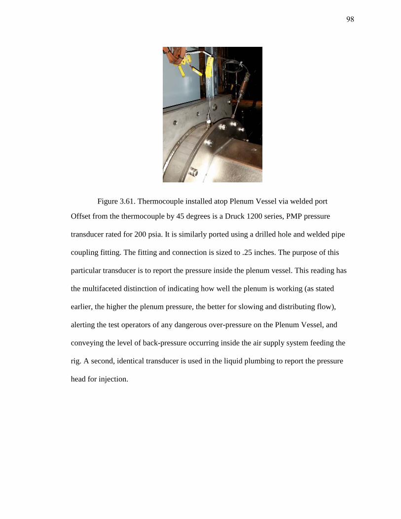
Figure 3.61. Thermocouple installed atop Plenum Vessel via welded port
Offset from the thermocouple by 45 degrees is a Druck 1200 series, PMP pressure
transducer rated for 200 psia. It is similarly ported using a drilled hole and welded pipe
coupling fitting. The fitting and connection is sized to .25 inches. The purpose of this
particular transducer is to report the pressure inside the plenum vessel. This reading has
the multifaceted distinction of indicating how well the plenum is working (as stated
earlier, the higher the plenum pressure, the better for slowing and distributing flow),
alerting the test operators of any dangerous over-pressure on the Plenum Vessel, and
conveying the level of back-pressure occurring inside the air supply system feeding the
rig. A second, identical transducer is used in the liquid plumbing to report the pressure
head for injection.
98

Figure 3.62. Pressure transducer ported and mounted to the Plenum Vessel
The high-speed infrared camera planned for flame visualization takes planar, mid-
spectrum infrared images. The camera contains a detector array whose sensitivity is aided
by cooling from liquid nitrogen poured and stored into a dewar inside the camera body.
Greater details of the camera set-up, operation, and maintenance are deliberately withheld
due to the restricted nature of certain camera features, but the camera does possess
multiple filters which allow species specific radiation intensity data to be obtained. Filters
for water vapor, carbon dioxide, and soot are all available with the camera.
99

Figure 3.63. The high speed infrared camera
3.11 Provisions for Complicating Flow Features Adaptability is essential for the functionality of the HSIC rig article. In that regard,
the rig is meant to be capable of going from the bare central cylindrical volume pictured
in figure 3.58 to a collection of features that more closely simulate the environment of an
aircraft engine nacelle. An advantage the HSIC test rig has over the Wright-Patterson
apparatus is the ability to gradually increment the complexity of the test section
environment. The Wright-Patterson experiment existed as a sharp binary: either a single,
1.5 inch diameter Inconel tube was used as the hot target surface, or a full third of a full
scale F-16 engine nacelle complete with a multi-stage bleed air duct, tubes, clamps, and
fuel pump. Gradually adding disturbances allows the effects of an individual feature to be
more accurately characterized. The sorts of features that have routinely been discussed in
Purdue’s interactions with Rolls-Royce have included: a flange-like feature to create a
step obstruction, tubing that winds along the Center Cylinder, and cylindrical
obstructions that extend into the annular gap of the test section. A recommended flange
component scaled to the test section of the HSIC rig is included in the engineering
drawings of appendix A.4. The dimensions for this part were concluded from interactions
with Rolls-Royce and were based on flanges typical to those used in extant turbofan
100

engine nacelles. Similar collaborative interactions should take place between Purdue and
Rolls-Royce to define dimensions for future flow components and configurations. In
anticipation of the need to secure all manner of parts to the Center Cylinder, 20 size ¼-20
threaded holes have been added. This size and tread were chosen for their ubiquity. The
feature attachment holes were also located sufficiently far downstream that the airflow
would have an opportunity to settle after passing through the Orifice Plate. The reference
by Pope [30] suggests a general settling distance of 100 hole diameters. This leaves the
airflow of the HSIC rig completely settled 9.35 inches into the test section with a buffer
of an extra inch before the flow features begin. When no feature is being attached to the
Center Cylinder, these holes must be treated with anti-seize and plugged to keep liquid
free of the passage for the electrical leads.
Figure 3.64. The plugged holes for flow features
101

3.12 Pressure and Temperature Rake A planned feature currently under development for the HSIC rig is a pressure-
temperature rake. The rake will serve a threefold purpose. It will be used to resolve the
thermal and fluid boundary layers of the air above the Hot Centerbody, and it will be
capable of giving in situ velocity measurements. The proposed rake design is presented
below:
Figure 3.65. Proposed design for the pressure-temperature rake
The base of the rake will have dimensions identical to the fused silica windows, but be
machined from stainless steel 304. This allows the rake to be secured to the HSIC rig
with the Window Flange feature and supports interchangeability between the rake and the
windows. The rake height extending into the test section gap is currently 1.2 inches. The
rake is also to be outfitted with 3 sensing nodes. Each node contains a type K
thermocouple to monitor temperature and a transducer to record stagnation pressure. A
static pressure measurement is to be made at the base of the rake. The in situ velocity
readings will be taken from comparing this static pressure measurement at the rake base
with the stagnation measurement taken at any of the sensing nodes. The rake is also to be
designed to withstand contact with both flames and liquid sprays. Discussions are
ongoing to leverage the rake design expertise of Aerodyn Engineering Inc. to realize this
component.
102

CHAPTER 4. PRELIMINARY TESTS
4.1 Flat Plate Test Article Experiments As an exercise in characterizing the ignition behavior of the flammable aircraft fluids
associated with the project, experiments were conducted using a simple flat plate test
article. This afforded the opportunity to acquire baseline reference data absent the
crossflow and curvature of the HSIC test rig and to practice infrared diagnostic methods.
The general experimental approach of Colwell et al. [8] and Shaw et al. [13] for droplet
ignition in a quiescent environment was followed. The fluids chosen for these
preliminary tests were the jet fuel, JP-8, and the hydraulic fluid, MIL-PRF-5606. They
were selected because they are the present-day iterations of JP-4 and MIL-H-5606, the
earliest fuels used on the Wright-Patterson test article. This chapter contains descriptions
of the flat plate apparatus, its test procedures, and the results from the preliminary
experiments with JP-8 and MIL-PRF-5606.
The experimental apparatus for the flat plate tests consisted of a heated stainless steel
plate surrounded by ceramic insulation. Drops of fuel were dispensed onto the plate from
above. The experimental arrangement is presented in its entirety in the figure below.
103

Figure 4.1. The complete experimental arrangement for the flat plate tests
The flat plate sits inside its white, high-temperature insulation at the center of figure
4.1. The plate is a 9 inch by 9 inch square of stainless steel which is bolted to a similarly
dimensioned square of copper. Five evenly spaced, .375 inch diameter, 1KW cartridge
heater elements are inserted into the copper in addition to the 5 type K thermocouples
that are wired to the heater controller. The high thermal conductivity of the copper plate
is leveraged to create a uniform temperature profile prior to conduction into the stainless
steel. As a consequence, the temperature profile within the stainless steel plate is
effectively isothermal. Five more thermocouples were embedded in the stainless steel and
wired to a data acquisition system to provide real time measurements of the hot surface
temperature.
104

Figure 4.2. Copper plate with installed cartridge heaters and bolt holes for the steel plate
Figure 4.3. Copper and stainless steel plates together with electrical leads
A programmable, 160 mL syringe pump was used to deposit metered droplets on the
stainless steel hot surface at regular intervals. Each drop had a volume of .25 mL. The
tubing and orifice delivering fuel to the surface from the pump were positioned such that
each drop fell a distance of 30 cm before impacting the stainless steel.
105

Figure 4.4. Syringe pump
A Phantom® series high speed camera was used to record droplet ignition at a rate of
3000 frames per second. This was used concurrently with the high-speed, nitrogen-cooled
infrared camera described in section 3.10 of the previous chapter.
At the start of each test day, the surface was treated with isopropyl alcohol to remove
any residues from the previous tests. It was discovered, however, that over the course of
several experiments, a plate would develop an oxide layer that fundamentally altered
ignition behavior. At this juncture, the plate was replaced. Isopropyl alcohol was also
used to prime and clean the vacuum pump and its attendant tubing. While the surface and
syringe pump were being cleaned, the high-speed infrared camera was centered, then
focused at a distance 34.5 inches from the edge of the stainless steel. The high speed was
positioned and angled so as to capture a top view of the flat plate surface. After the
cleaning, the syringe pump was loaded with the test fluid, and the temperature controller
was set near its auto-ignition temperature. For each temperature set point, 20 drops were
dispensed onto the center of the plate surface at time intervals that allowed each drop to
completely vaporize before the next one fell. The repeated drops at each set point
conforms to the probabilistic understanding of hot surface ignition put forth by Colwell
[8]. The plate temperature was initially raised in 100°C increments until the first ignition
106
was achieved. After first ignition, the set temperature was lowered by 50°C, and the drop
series was begun anew. Temperature was raised in 10°C increments from this point
onwards with the number of ignited drops at each set point being recorded by the test
conductors. Tests were concluded when a 100% ignition probability had been
demonstrated for two successive set temperatures. Throughout this process, the
temperature being monitored was that of the stainless steel plate. This was in contrast to
the temperature integrated into the controller feedback, which was read from the copper.
Despite the emphasis placed on temperature uniformity in the experimental arrangement,
the differing thermal conductivities of the steel and copper led to a natural discrepancy
between the two plate temperatures. Time was therefore granted after each set point, to
permit the individual plate temperatures to stabilize. During tests, the temperature of the
steel was found to be roughly 50°C cooler than the copper. Due to the highly transient
nature of the flames observed for droplet ignition, data was not taken on either of the
high-speed cameras until the probability of ignition reached 100%. Data acquisition had
to be triggered manually, so a principle of selective camera use was followed to
maximize the potential for a captured flame. Because the generated files on both cameras
were also quite large, this had the secondary effect of greatly reducing the storage space
necessary for data management.
In broad agreement with the literature, the minimum hot surface ignition temperature
demonstrated for both JP-8 and MIL-PRF-5606 were at least 400°C higher than their
reported auto-ignition temperatures. The auto-ignition temperature of JP-8 is 223°C, but
hot surface ignition was not achieved until the steel reached 676°C. Likewise, the auto-
ignition temperature for MIL-PRF-5606 is 218°C, but no ignition was observed until the
107

plate was at 650°C. Visible images for the 100% ignition points of both JP-8 and MIL-
PRF-5606 are shared in figure 4.5 and figure 4.6 respectively. Also in general agreement
with the results from the literature, was the face that MIL-PRF-5606 proved to be slightly
easier to ignite than JP-8 [5]. It reached both the initial and 100% ignition probability
points approximately 15°C sooner.
Figure 4.5. JP-8 ignition at 737±2°C and 100% ignition probability
Figure 4.6. MIL-PRF-5606 ignition at 721±2°C and 100% ignition probability
108

A logistic regression curve fit [8] was performed to translate the raw data into a hot
surface ignition temperature probability curve.
𝑃𝑃(𝑌𝑌) = exp (𝑏𝑏𝑜𝑜+𝑏𝑏1.𝑅𝑅)1+exp (𝑏𝑏𝑜𝑜+𝑏𝑏1.𝑅𝑅)
[Eq. 4-1]
The coefficients b0 and b1 were based on the two temperature points with the lowest
observed ignition probability and the highest observed ignition probability less than
100%. A MATLAB script was used to aid in the computation. The results from the JP-8
and MIL-PRF-5606 tests are presented in the following tables and figures.
Table 4.1. Ignition Data for JP-8
Set temperature in copper plate (°C)
Mean temperature in Stainless steel
plate (°C)
Standard deviation of Stainless steel temperature (°C)
Ignition probability
600 556 4 0
700 651 3 0
710 659 4 0
720 668 3 0
730 676 3 0.1
740 685 3 0.2
750 693 5 0.4
760 702 4 0.75
770 711 4 0.75
780 720 5 0.85
790 728 3 0.9
800 737 3 1
810 746 4 1
The coefficients for JP-8 were b0 = -59.325 and b1 = 0.084°C-1.
109

Figure 4.7. Ignition probability curve for JP-8
Table 4.2. Ignition Data for MIL-PRF-5606
Set temperature in copper plate (°C)
Mean temperature in Stainless steel
plate (°C)
Standard deviation of Stainless steel temperature (°C)
Ignition probability
600 560 3 0
700 650 3 0.10
710 659 3 0.20
720 668 4 0.35
730 676 4 0.60
740 685 4 0.65
750 694 4 0.80
760 704 4 0.90
110

Table 4.2 cont. 770 713 5 0.95
780 721 3 1.00
790 730 4 1
The coefficients for MIL-PRF-5606 were b0 = -55.246 and b1 = 0.081°C-1.
Figure 4.8. Ignition probability curve for MIL-PRF-5606
That the MIL-PRF-5606 ignited more readily than JP-8 is consistent with the finding by
Johnson et al. [5] of the hydraulic fluid exhibiting a lower minimum ignition temperature
for a variety of experimental conditions. This was at least partially attributed to the more
viscous character of the hydraulic fluid and is also reflected in its higher overall
flashpoint (89°C vs 48°C for JP-8) [5]. It was described in the literature review chapter
111

how ignition represents a competition between chemical rates and environmental
conditions. With its higher viscosity, MIL-H-5606 would be more resistant to transport
away from the heat source after being deposited. With its higher flashpoint, MIL-H-5606
would be less likely to evaporate early and more inclined to steadily collect in
proportions conducive to flammability. It was noted with the simple duct test article at
Wright-Patterson how the inclusion of even a single flow obstruction such as a cushion
clamp lowered the minimum ignition temperature for MIL-H-5606 more dramatically
than for than the less viscous, more volatile kerosene based JP-4 and JP-8 [5].
Supplementing the basic ignition probability data taken from these experiments were
infrared images.
Figure 4.9. Instantaneous image of JP-8 ignition at 810°C set point for 2.58±.03µm
112

Figure 4.10. Instantaneous image of MIL-PRF-5606 ignition at 780°C set point for 2.58±.03µm
The wavelength range given in figures 4.9 and 4.10 corresponds to soot and water vapor
species and the scale, D, is equal to 8mm. The images are reported in terms of the
radiation intensity received from the targeted source with sr signifying the solid angle
through which the signal is transmitted. The average spatial radiation intensity from the
JP-8 flame is higher than that of MIL-PRF-5606. Higher energy density is to be expected
considering its primary use as fuel. Herein lies the added diagnostic potential of infrared
imagery. Although these images only give conclusive information on the radiation
intensity of the sample, the radiation intensity correlates with the overall temperature
and/or energy state of the filtered species. The temperature of product species is crucial to
understanding the thermal formation of undesirable chemical species such as soot and
NOx [31]. Consequently, radiation intensity serves as an indirect measure of soot
formation, oxidation, and emissions [31]. An issue that arose when acquiring the infrared
113

images of JP-8 and MIL-PRF-5606 was linked to the transient nature of droplet ignition.
The flames evolved from the drop contacting the surface only lasted on the order of a few
hundred milliseconds. There was ample time for the acquisition rate of the high speed
infrared camera, but coordination was problematic for the camera operator having to
trigger the recording (this was less of an issue with the Phantom® series camera since the
output file includes the last few seconds prior to the trigger as a matter of function).
Further complicating matters was the varied ignition delay time for the different test
fluids. Johnson et al. noted the ignition delay time for MIL-H-5606 to be approximately 3
times that of JP-8 [5]. Direct comparison across separate trials, even for the same test
fluid, carried the disadvantage of the acquired images falling at different edges of the
flame lifetime. The general approach for capturing droplet ignition was to first take
multiple recordings at the 100% probability point, then later sort through the data during
post processing for the captured flame. These difficulties do not necessarily preclude hot
surface ignition from more nuanced infrared work in the future. An alternative to
manually triggering data acquisition could have the infrared camera in loop with a UV
flame detector so that trigger response is tied directly to ignition. Another alternative
would be to reconfigure data acquisition so that generated files include more of the time
elapsed prior to triggering. On the larger scale HSIC test rig, a natural corrective seemed
to present itself. Since fuel injection on the HSIC rig is designed to exist as a sustained
leak for approximately 5 seconds, greater quantities of flammable fluid are present. Thus,
the flames seen during the earliest experiments to benchmark the test rig were larger and
tended to linger on the order of seconds prior to either self-extinguishment or blow-out
from the nitrogen purge. Infrared imagery remains a promising avenue for future
114
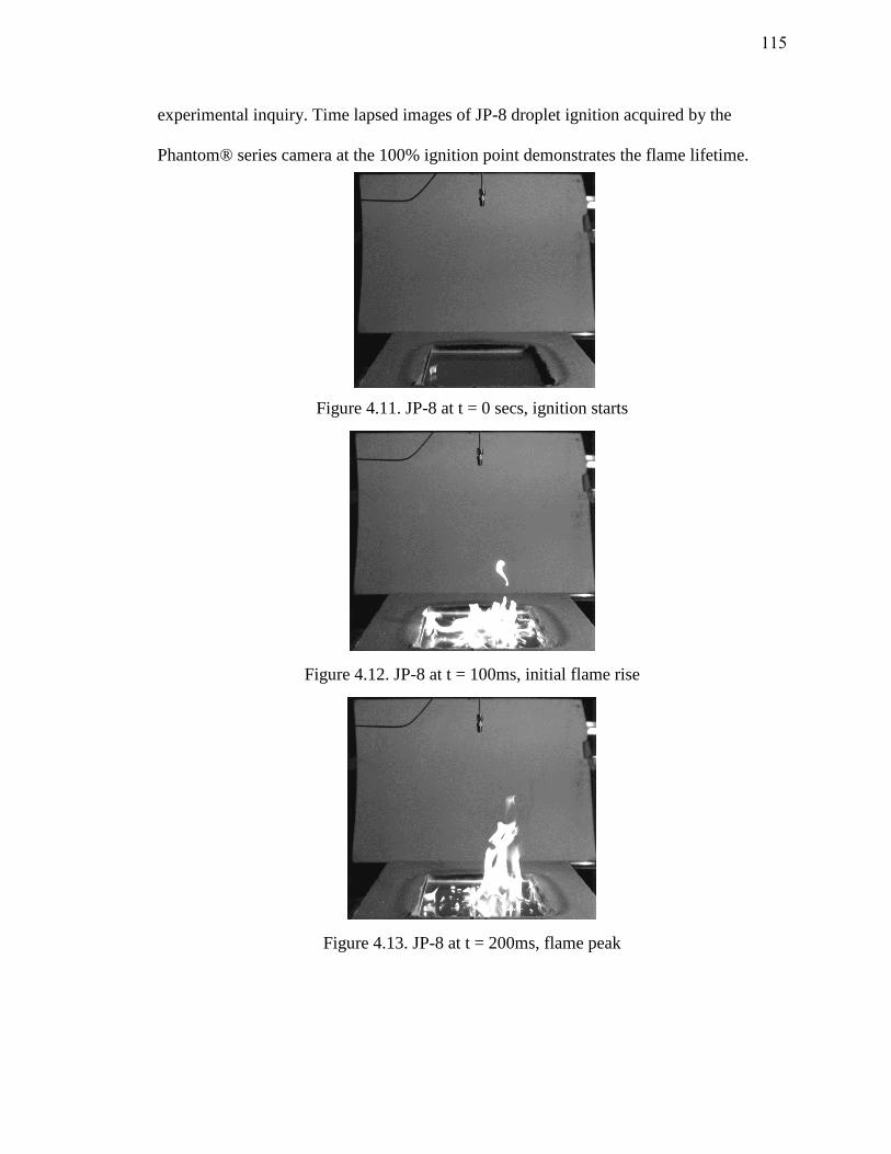
experimental inquiry. Time lapsed images of JP-8 droplet ignition acquired by the
Phantom® series camera at the 100% ignition point demonstrates the flame lifetime.
Figure 4.11. JP-8 at t = 0 secs, ignition starts
Figure 4.12. JP-8 at t = 100ms, initial flame rise
Figure 4.13. JP-8 at t = 200ms, flame peak
115

Figure 4.14. JP-8 at t = 300ms, flame diminishing prior to extinction
4.2 Simple Cylinder Tests Work was also done to vet the capabilities of the cartridge heater elements settled on
for the Hot Centerbody of the HSIC rig. To that effect, a 3 inch diameter, 6 inch long rod
of stainless steel 304 was machined to accept a .5 inch diameter, 1 KW cartridge heater
element nearly identical to those used in the Hot Centerbody (it lacked lead protection).
A K type thermocouple was tack-welded to the surface and then directly connected to the
temperature controller feedback. For this reason, only the temperature of the controller
reading had to be monitored during the course of the experiment. In order to take
advantage of the extant flat plate apparatus while avoiding facility damage, coarse blocks
of porous ceramic insulation were stacked over the stainless steel plate for the cylindrical
test article. A final bed of ceramic fiber wool was laid on top of the porous ceramic, and
served as the resting place for the cylinder. The first tests done were those to exercise the
cartridge heater.
116

Figure 4.15. Cylindrical test article atop porous ceramic block and ceramic fiber bedding
Figure 4.16. Cylindrical test article at a 650°C set point
117

Figure 4.17. Cylindrical test article at a 1000°C set point
As shown in figure 4.17, the single heater element was able to bring the temperature of
the stainless steel cylinder up to 1000°C (or 1832°F). This temperature is at the absolute
upper end of the design envelope and was viewed as a final justification for the chosen
heater elements. Greater confidence in the suitability of the cartridge heaters was derived
from the realization that an individual element was able to take 12 lbs. of stainless steel
(which exhibits a similar thermal conductivity to Inconel 718) to the maximum design
temperature. This is compared against the Hot Centerbody component, which has a total
mass of 22.63 lbs and a total of 15 available kilowatts for a mass loading of 1.5 lb./KW.
The thermal load borne by an individual element inside the actual target surface is
therefore considerably less than the heater limit at quiescent conditions.
In an effort to quantify the effects of surface curvature on the hot surface ignition
temperature, the flat plate experiment for JP-8 was repeated with the heated cylindrical
test article. In was observed during testing that the ceramic fiber wool used as bedding
had a tendency to absorb the fuel droplets that were not completely vaporized by the
118

cylinder. In the event of a drop ignition, the soaked ceramic wool around the edges of the
cylinder would also catch fire, and prolong the flame duration. The Phantom® high-
speed camera was used to confirm that ignition began on the surface of the cylinder.
Figure 4.18. JP-8 on the cylinder at t = 0s, ignition starts
Figure 4.19. JP-8 on the cylinder at t = 110ms, flame propagates along cylinder length
119

Figure 4.20. JP-8 on the cylinder at t = 220ms, flame catches on the ceramic wool
Figure 4.21. JP-8 on the cylinder at t = 330ms, flame is prolonged by stabilization on the wool
The burning ceramic compromised the infrared images acquired for the cylinder, but the
raw ignition probability data remained viable.
Table 4.3. Ignition Data for JP-8 on the cylindrical test article
Temperature (°C) Ignited drops Ignition probability
300 0 0 400 0 0 500 0 0 550 0 0
120

Table 4.3 cont. 600 0 0 650 0 0 675 0 0 695 3 0.3 700 5 0.5 705 5 0.5 710 6 0.6 715 8 0.8 720 10 1 750 10 1 800 10 1
The coefficients for JP-8 on the cylinder were b0 = -96.96 and b1 = 0.1379.
Figure 4.22. Ignition probability data for JP-8 on the cylindrical test article The
start of the ignition probability curve in figure 4.22 is shifted over to the right from
figure 4.7. The suggestion is that increasingly convex surface curvature has the effect of
121

raising the minimum hot surface ignition temperature. Considering that convex curvature
would have the effect of forcing liquid drops to slide down the sides of any given surface,
reducing their residence time near the ignition source, the result is to be expected. In fact,
the curvature of the HSIC rig, and the irregular surface geometries of the engine nacelle
environment in general, suggests that the barriers to hot surface ignition will only be
higher in more realistic applications.
122

CHAPTER 5. VALIDATING THE RIG
5.1 Initial Test with Propane Although the design and fabrication of the HSIC test rig preoccupies the majority of
this thesis work, the validation of its operation was also undertaken. The work described
throughout this brief chapter reflects the HSIC in its baseline configuration. No effort was
made to include flow complicating features at this stage of experiments since the first
opportunity for data continuity lies in reproducing the results from the Simple Bare Duct
[5] test article of the Wright-Patterson rig. In addition to flowing air up to rates near .5
lb/s, tests were conducted with propane and JP-8 to confirm the rig’s ability to ignite fuel
and to begin the process of reproducing then extending the data gathered from the
Wright-Patterson test articles.
The first attempted data collection on the HSIC rig was for tests with propane.
Propane was selected to confirm the HSIC rig’s ability to ignite hydrocarbon fuel based
on the spray behavior observed by Graves [15] during hot surface experiments in a
vertical duct. As discussed, in the literature review chapter, the genuine kerosene fuels
used by Graves tended to atomize poorly, and pool in undesirable regions of the test
apparatus. Graves noted that propane, which readily flashes at room temperature, acted as
a more flammable surrogate for a well-atomized kerosene spray. When conducting the
earliest experiments on the HSIC rig with propane, the intention was to identify then
minimize any fundamental shortcomings of the apparatus without immediately exposing
123

the hardware to the risk of liquid collecting in hazardous quantities inside the test section.
The propane tests led to successful ignition for an Inconel surface temperature of
782±3°C at an air velocity of .45±.05 m/s and an air temperature of 104±12°C. Propane
was injected through the open end of a .125 inch stainless steel tube with .028 inch wall
thickness. The pressure driving injection was roughly 60 psia in accordance with the
approximate vapor pressure of propane on the day of testing, October 30, 2015 (12°C). A
complete test matrix for the propane tests is provided in the table below.
Table 5.1 Propane Test Matrix, October 30, 2015
Air Mass Flow,
kg/s
Surface Temp., °C Air Temp., °C Air Velocity,
m/s
Ignition?
.016±.002 kg/s 427±3°C 94±12°C .55±.05 m/s No
.015±.002 kg/s 482±3°C 80±12°C .51±.05 m/s No
.020±.001 kg/s 482±3°C 82±12°C .69±.04 m/s No
.012±.002 kg/s 538±3°C 96±12°C .40±.05 m/s No
.023±.001 kg/s 538±3°C 84±12°C .78±.04 m/s No
.044±.001 kg/s 538±3°C 89±12°C 1.46±.01 m/s No
.012±.002 kg/s 649±3°C 86±12°C .41±.05 m/s No
.022±.001 kg/s 649±3°C 83±12°C .72±.04 m/s No
.044±.001 kg/s 649±3°C 86±12°C 1.46±.01 m/s No
.011±.002 kg/s 704±3°C 100±12°C .37±.05 m/s No
.022±.001 kg/s 704±3°C 93±12°C .72±.04 m/s No
.043±.001 kg/s 704±3°C 93±12°C 1.44±.01 m/s No
124

Table 5.1 cont.
.064±.004 kg/s 704±3°C 118±12°C 2.13±.06 m/s No
.014±.004 kg/s 760±3°C 122±12°C .46±.05 m/s No
.013±.004 kg/s 782±3°C 104±12°C .45±.05 m/s Yes
.013±.004 kg/s 782±3°C 84±12°C .44±.05 m/s Yes
.013±.004 kg/s 782±3°C 77±12°C .44±.05 m/s Yes
The propane flowrate in throughout these tests was approximately 17.3 ml/s, or slightly
more than twice the standard flowrate of the Wright-Patterson test article for a duration of
5 seconds. This was permitted since the objective of the propane test was merely to verify
ignition, not the reproduction of any particular data point.
5.2 Initial Tests with JP-8 Once ignition was demonstrated with propane, testing shifted toward recreating and
augmenting data points taken on the Wright-Patterson test rig. The first fluid chosen for
testing was JP-8. This was done to approximate the initial tests performed on the Simple
Bare Duct test article of the Wright-Patterson experiment with JP-4. JP-8 was used in lieu
of JP-4 due to the latter having been phased out of use because of its high volatility and
tendency to build static charge at ambient, vaporous conditions. The .125 inch, stainless
steel tubing was capped at its open end with a misting nozzle with an 80 degree spray fan
and a .016 inch diameter orifice. The nozzle was installed to more precisely control the
liquid flowrate to the test section and can be seen beside the glowing Inconel target in the
subsequent photograph.
125

Figure 5.1 Test article heated to 843±3°C with spray nozzle visible
The nozzle produces droplets in the 50 micron range (consistent with the expected
droplet size of the Wright-Patterson rig), and was injected at the scaled rate of 1.1 mL/s
for a duration of 5 seconds with a driving pressure of 125 psia. Ignition was first achieved
at a surface condition of 843±3°C. The air velocity was .35±.01 m/s and the air
temperature was 106±15°C. The results are summarized in the table below.
Table 5.2 JP-8 Test Matrix, October 31, 2015
Air Mass Flow,
kg/s
Surface Temp., °C Air Temp., °C Air Velocity,
m/s
Ignition?
.012±.001 kg/s 704±3°C 62±15°C .41±.03 m/s No
.013±.001 kg/s 704±3°C 88±15°C .44±.03 m/s No
.011±.001 kg/s 732±3°C 81±15°C .37±.03 m/s No
.011±.001 kg/s 732±3°C 75±15°C .37±.03 m/s No
.023±.001 kg/s 760±3°C 66±15°C .75±.02 m/s No
.023±.001 kg/s 760±3°C 68±15°C .75±.02 m/s No
126

Table 5.2 cont.
.011±.001 kg/s 760±3°C 70±15°C .35±.03 m/s No
.010±.001 kg/s 760±3°C 68±15°C .34±.03 m/s No
.022±.001 kg/s 788±3°C 71±15°C .75±.02 m/s No
.041±.001 kg/s 788±3°C 86±15°C 1.38±.02 m/s No
.041±.001 kg/s 816±3°C 101±15°C 1.38±.02 m/s No
.064±.001 kg/s 816±3°C 107±15°C 2.13±.02 m/s No
.011±.001 kg/s 816±3°C 106±15°C .37±.03 m/s Yes
.011±.001 kg/s 816±3°C 101±15°C .37±.03 m/s Yes
.021±.001 kg/s 816±3°C 96±15°C .72±.02 m/s Yes
.021±.001 kg/s 816±3°C 93±15°C .72±.02 m/s Yes
The first observed ignition for JP-8 on the baseline HSIC rig configuration is 38°C higher
than the first observed ignition temperature for JP-4 [5]. This is consistent with JP-8’s
implementation as a less flammable version of JP-4.
Figure 5.2 JP-8 ignition for 816±3°C at 106±15°C air temperature and .37±.03 m/s air velocity
127

It is evident from figure 5.2 that the flame initiated at the Inconel surface very quickly
propagates back to the nozzle head. This was a result of the flame speed easily exceeding
the air velocity at these low flow rates and the nozzle face being placed too close to the
Inconel target (~2mm away). Also gathered from these initial tests was the considerable
drift in the measured air temperature. This was reduced notably in later experimental
trials as the testing became more streamlined, and the researchers gained greater
familiarity with the response of the rig’s systems.
To more closely observe the degree to which air temperature and air velocity
affect the hot surface ignition temperature, a new flight of data was targeted for the
elevated air temperature of 149°C. This serves as the first new addition to the hot surface
ignition database established at Wright-Patterson by more closely observing the
fundamental effects elevated temperature and velocity have on JP-8 sprayed upstream of
the hot surface. Under a modified test arrangement, JP-8 is now sprayed 6.5 inches
upstream of the surface leading edge and is directly ported into the wall of the Octagonal
Duct. This has the effect of forcing the flame to travel farther to propagate to the nozzle
face and allowing the injectant spray more space to atomize and distribute inside the test
section. The liquid flowrate and duration is unchanged from the previous experiment,
remaining 1.1 mL/s and 5 seconds respectively.
128

Table 5.3 JP-8 Test Matrix, December 14, 2015
Air Flow, kg/s Surface Temp., °C Air Temp., °C Air Vel., m/s Ignition?
0.008±.001 kg/s 593±3°C 145±3°C 0.30±.02 m/s No
0.008±.001 kg/s 621±2°C 148±3°C 0.31±.02 m/s Yes
0.017±.001 kg/s 617±2°C 150±3°C 0.64±.03 m/s No
0.008±.001 kg/s 649±3°C 151±3°C 0.30±.02 m/s Yes
0.017±.001 kg/s 648±3°C 148±3°C 0.67±.03 m/s No
0.031±.001 kg/s 644±3°C 149±3°C 1.19±.03 m/s No
0.008±.001 kg/s 667±2°C 153±3°C 0.30±.02 m/s Yes
0.017±.001 kg/s 667±2°C 148±3°C 0.67±.03 m/s No
0.032±.001 kg/s 670±2°C 147±3°C 1.23±.03 m/s No
0.048±.005 kg/s 672±2°C 154±3°C 1.85±.02 m/s No
0.063±.005 kg/s 667±2°C 155±3°C 2.44±.01 m/s No
0.008±.001 kg/s 694±3°C 147±3°C 0.30±.02 m/s Yes
0.016±.001 kg/s 697±3°C 149±3°C 0.60±.03 m/s Yes
0.033±.001 kg/s 694±3°C 149±3°C 1.28±.03 m/s No
0.047±.005 kg/s 702±3°C 153±3°C 1.80±.02 m/s No
0.063±.001 kg/s 698±3°C 150±3°C 2.44±.01 m/s No
0.008±.001 kg/s 723±2°C 147±3°C 0.30±.02 m/s Yes
0.017±.001 kg/s 728±3°C 150±3°C 0.67±.03 m/s Yes
0.031±.001 kg/s 727±3°C 150±3°C 1.20±.03 m/s No
129

Table 5.3 cont.
0.048±.005 kg/s 723±3°C 152±3°C 1.85±.02 m/s No
0.063±.001 kg/s 728±3°C 151±3°C 2.45±.01 m/s No
0.008±.001 kg/s 757±2°C 147±3°C 0.32±.02 m/s Yes
0.016±.001 kg/s 762±2°C 148±3°C 0.60±.03 m/s Yes
0.032±.001 kg/s 757±2°C 148±3°C 1.24±.03 m/s No
0.048±.005 kg/s 757±2°C 152±3°C 1.84±.02 m/s No
0.063±.001 kg/s 760±2°C 152±3°C 2.44±.01 m/s No
0.008±.001 kg/s 788±3°C 147±3°C 0.30±.02 m/s Yes
0.016±.001 kg/s 786±3°C 149±3°C 0.62±.03 m/s Yes
0.031±.001 kg/s 792±3°C 150±3°C 1.21±.03 m/s Yes
0.048±.005 kg/s 787±3°C 150±3°C 1.84±.02 m/s No
0.063±.005 kg/s 783±3°C 150±3°C 2.44±.01 m/s No
0.016±.001 kg/s 813±3°C 149±3°C 0.62±.03 m/s Yes
0.032±.001 kg/s 813±3°C 149±3°C 1.24±.03 m/s Yes
0.048±.005 kg/s 813±3°C 149±3°C 1.84±.02 m/s Yes
0.063±.005 kg/s 813±3°C 151±3°C 2.45±.01 m/s No
0.032±.001 kg/s 839±3°C 148±3°C 1.22±.03 m/s Yes
0.048±.005 kg/s 843±3°C 151±3°C 1.84±.02 m/s Yes
0.063±.005 kg/s 845±3°C 151±3°C 2.45±.01 m/s Yes
0.048±.005 kg/s 874±5°C 148±3°C 1.84±.02 m/s Yes
0.063±.005 kg/s 867±5°C 151±3°C 2.45±.01 m/s Yes
130

The results shared in table 5.3 can be used to draft a plot for the minimum hot surface
ignition temperature of JP-8 at 149°C as a function of air velocity.
Figure 5.3 Effect of air velocity on MHSIT of JP-8 at 149°C air temperature
A clear positive correlation between increasing air velocity and increasing hot surface
ignition temperature is displayed in the figure. This is justified in the bulk air velocity
dominating the trajectory and motion of the fuel spray (as described in section 3.8). At
higher bypass air velocities, the momentum ratio between the injected fluid and the
crossflow skews more heavily in favor of the crossflow, making it more difficult for
individual fuel droplets to reach the surface. Furthermore, those fuel drops that do reach
the surface are still subject to the bulk motion of the air, and are consequently dragged or
pulled from the target hot surface more quickly at the faster flow conditions. A non-
131

dimensional parameter for hot surface ignition suggested by this behavior is the
Damköhler number, Da, which is the ratio of the residence time of a given reactant to its
chemical reaction time [31]. The residence time can either be estimated numerically or
with high speed imagery to track the time scale of droplet contact with the Inconel
surface. The chemical rate is more elusive, although an ignition delay time observed
during tests on the quiescent flat plat may provide an experimental basis for such a value.
The effect of the elevated air temperature is reflected in the contrast between the
minimum hot surface ignition temperature for 1 ft/s of air at 149°C and the earlier tests
with air at the same velocity and 83°C. For those earlier tests, the JP-8 spray did not
ignite until the surface reached 816°C vs 621°C for the later experiments. This is
supported by Johnson et al.’s [5] findings that increased air temperature generally
lowered the ignition temperature. It is also noted that the probabilistic range observed by
Colwell et al. [8] for the quiescent flat plate experiments was not observed at all for the
HSIC rig. It is theorized that the more aggressive flow environment inside of the HSIC,
and similar rigs raises the overall barrier to ignition to the point that the ignition threshold
is more definitively set. Considerable work lies ahead to more fully explore hot surface
ignition phenomena, but these early results are encouraging that thorough
experimentation with the HSIC test rig may yield some insight.
132

CHAPTER 6. CONCLUSIONS AND FUTURE WORK
The work reported in this thesis involved the design, construction, and preliminary
experimentation for improved understanding of hot surface ignition in an environment
representative of an aircraft engine. Future work will systematically change the air flow
path through the rig test section to resemble engine nacelle environments and understand
the effects of unique features. Previous researchers reported that fuel leak flow rates had
little to no effect on the minimum hot surface ignition temperature [5]. The broader range
of air flowrates designed for the HSIC rig will allow an investigation of the lean and rich
flammability limits associated with a combination of the fuel leak rate and the airflow
rate to describe an envelope of safe operating conditions.
Future work will involve cluttered engine compartments and complexities associated
with the confluence of multiple boundary layers, wakes and pressure gradients. The bulk
fluid velocity, fluid temperature, surface roughness, surface temperature, leak type (spray
or stream), and state of fuel vaporization will all affect ignition. The number of potential
test variables is in fact, so large that future work will have to involve systematic non-
dimensional analysis and computational combustion studies to define the most relevant
experimental conditions. The experimental apparatus described in this thesis has laid the
foundation for the design of future studies aimed at continuous improvements in the fire
safety of modern aircraft engines.
133

LIST OF REFERENCES

LIST OF REFERENCES
[1] L. Strawhorn, “Motor Vehicles,” in Fire Protection Handbook, Quincy, MA: National Fire Protection Association, 2003, Section 14, Chapter 1.
[2] National Transportation Safety Board, “Aircraft Accident Report: In-flight Breakup Over the Atlantic Ocean Trans World Airlines Flight 800,” August 23, 2000.
[3] ASTB Final Investigation Report, AO-2010-089, “In Flight Uncontained Engine Failure Overhead Batam Island, Indonesia 4 November 2010,” VH-OQA Airbus A380-842
[4] Drew, K. and Clark, N., “3 Airlines Halt A380 Flights Over Engine Explosion,” The New York Times, The New York Times, 4 Nov. 2010. Web 3 Jul. 2014
[5] Johnson, A.M., Roth, A.J., and Moussa, N. A., “Hot Surface Ignition Tests of Aircraft Fluids,” Air Force Wright Aeronautical Laboratories, AFWAL-TR-88-2101, Wright Patterson Air Force Base, OH, 1989
[6] Khamliche, Y., “Flammable Fluid Hot Surface Ignition,” PowerPoint Presentation given March 31, 3014 at Rolls Royce Corporation at 450 S Meridian St., Indianapolis, IN
[7] Davis, S., Kelly, S., and Somandepalli, V., “Hot Surface Ignition of Performance Fuels,” Fire Technology, Vol. 46, 2010, pp.363-374.
[8] Colwell, J. D., and Reza, A., “Hot Surface Ignition of Automotive and Aviation Fluids,” Fire Technology, Vol. 41, 2005, pp.105–123.
[9] Davis, S., and Somandepalli, V., “Hot Surface Ignition of Ethanol, Gasoline, E-85, Diesel, and E-Diesel,” AIChE, 2007 Spring Meeting & 3rd Global Congress on Process Safety, 27th April 2007, Houston, TX.
[10] Kuchta, J. M., “Summary of Ignition Properties of Jet Fuels and Other Aircraft Combustible Fluids,” Air Force Aero Propulsion Laboratories, AFAPL-TR-75-70, Wright Patterson Air Force Base, OH, 1975
[11] ASTM Standard E659, 2014, “Standard Test Method for Autoignition Temperature of Liquid Chemicals,” ASTM International, West Conshohocken, PA, DOI: 10.1520/E0659, www.astm.org
134

[12]Gottried B.S., Lee, C. J., and Bell, K.J., “The Leidnenfrost Phenomenon: Film Boiling of Liquid Droplets on a Flat Plate,” International Journal of Heat and Mass Transfer, Vol.9, 1966, pp. 1167-1187
[13] Shaw, A., Epling, W., McKenna, C., and Weckman, B., “Evaluation of the Ignition of Diesel Fuels on Hot Surfaces,” Fire Technology, Vol. 46, 2010, pp.407-423
[14] Myronuk, D.J., “Dynamic, Hot Surface Ignition of Aircraft Fuels and Hydraulic Fluids,” Air Force Wright Aeronautical Laboratories, AFWAL-TR-79-2095, Wright Paterson Air Force Base, OH, 1980
[15] Graves, C.B., “Spray Ignition by a Hot Surface,” MS Thesis, Purdue University, West Lafayette IN, 1984
[16] Ingerson, D., “Engine Nacelle Halon Replacement,” FAA WJ Hughes Technical Center, Fire Safety Section AAR-422, Atlantic City International Airport, NJ, June 2002
[17] Smits, A. J., A Physical Introduction to Fluid Mechanics, John Wiley, New York, NY, 2000
[18] Bergman, T. L., Lavine, A. S., Incropera, F. P., and Dewitt, D. P., Fundamentals of Heat and Mass Transfer 7th Edition, John Wiley & Sons, Hoboken, NJ, 2011
[19] Greene, G. A., Finfrock, C. C., and Irvine Jr., T. F., “Total Hemispherical Emissivity of Oxidized Inconel 718 in the Temperature Range 300-1000°C,” Experimental Thermal and Fluid Science, Vol. 22, Issues 3-4, 2000, pp.145-153
[20] Budynas, R. G., and Nisbett, J. K., Shigley’s Mechanical Engineering Design 9th Edition, McGraw-Hill, New York, NY, 2010
[21] Special Metals, “Inconel 718 Alloy,” Publication Number SMC-045, Sept. 2007
[22] Professional Plastics, “Ceramic-Comparative Material Data Sheets,” Retrieved Mar. 2015
[23] Sutton, G. P., and Biblarz, O., Rocket Propulsion Elements 8th Edition, John Wiley & Sons, Hoboken, NJ, 2010
[24] Kolodize Jr., P. A., and Winkle, M. V., “Discharge Coefficients Through Perforated Plates,” American Institute of Chemical Engineers Journal, Vol. 3, No. 3, Sept. 1957, pp. 303-312
[25] Miracrys, “Sapphire,” Miracrys, 2007. [Online] Available: http://www.miracrys.com/CCinit.php?id=productsa [Accessed: Mar. 2015]
135

[26] Electron Microscopy Sciences, “Technical Data Sheets-GE 124 Quartz,” Electron Microscopy Sciences, 2015. [Online] Available: https://www.emsdiasum.com/microscopy/technical/datasheet/GE124.aspx [Accessed: Mar. 2015]
[27] GrafTech, “Grafoil® Engineering Design Manual 2nd Edition,” 2002
[28] Guildenbecher, D. R., “Droplet Physics,” School of Mechanical Engineering, Purdue University, West Lafayette, IN, Jan. 18, 2010
[29] O’Keefe Controls Co., “Choked Flow of Gases,” O’Keefe Controls Co., Trumbull, CO, 2003
[30] Pope, S.B., Turbulent Flows. Cambridge: Cambridge University Press, 2000. Print
[31] Turns, S. R., An Introduction to Combustion: Concepts and Applications 3rd Edition, McGraw-Hill, New York, NY, 2012
[32] Bennett, J. M., and Ballal, D.R., “Ignition of Combustible Fluids by Heated Surfaces,” AIAA, 41st Aerospace Sciences Meeting and Exhibit, 6-9 January 2003, Reno, NV
[33] 4. Ramos, J.I., “Ignition of Confined Gaseous Mixtures by Hot Surfaces and Hot Wires,” AIAA, 21st Aerospace Sciences Meeting, 10-13 January 1983, Reno, NV
[34] Graves, C.B., Tang, Y.L., and Skifstad, J.G., “Ignition of a Fuel Spray by a Hot Surface,” AIAA 21st Joint Propulsion Conference, 8-10 July 1985, Monterey, CA.
[35] Parts, L., and Olt, R.G., “High Temperature (1649ºC, 3000ºF) Surface Ignition Test Apparatus for Fluids,” Air Force Wright Aeronautical Laboratories, AFWAL-TR-82-2110, Wright Paterson Air Force Base, OH, 1983
[36] Kumar, R.K., “Ignition of Hydrogen-Oxygen-Diluent Mixtures Adjacent to a Hot, Nonreactive Surface,” Combustion and Flame, Vol. 75, 1989, pp.197-215.
[37] Geyer, W.H., and Moussa, N.A., “Hot Surface Ignition and Fire Suppression Tests in an Aircraft Engine Bay,” 27th Joint Propulsion Conference, AIAA, Sacramento, CA, 1991
[38] Dehong, K., Eckhoff, R.K., and Alfert, F., “Auto-Ignition of CH4/air, C3H8/air, and CH4/CO2/air using a 1 L Ignition Bomb,” Journal of Hazardous Materials, Vol. 40, 1995, pp. 69-84
[39] Menon, S.K., Boettcher, P.A., Ventura, B., Sheperd, J.E., and Blanquart, G., “Modeling Hot-Surface Ignition of Hydrocarbon-Air Mixtures,” 7th US National Technical Meeting of the Combustion Institute Hosted by the Georgia Institute of Technology, Atlanta, GA March 20-23, 2011
136

[40] Reid, I.A.B., Robinson, C., and Smith, D.B., “Spontaneous Ignition of Methane: Measurement and Chemical Model,” Twentieth Symposium (International) on Combustion/The Combustion Institute, 1984, pp. 1833-184
[41] Sano, T., and Yamashita, A., “Flame Ignition of Premixed Methane Air Mixtures on a High-Temperature Flat Plate,” JSME International Journal, Series B, Vol. 37, No. 1, 1994
[42] Skifstad, J.G., Lefebvre, A.H., and Murthy, S.N.B., ”Fuel Spray Ignition by Hot Surfaces and Aircraft Fire Stabilization,” Air Force Office of Scientific Research, AFOSR-TR-86-0856, Purdue University-West Lafayette, IN, October 1986
[43] Hamins, A., and Borthwick, P. “Suppression of Ignition over a Heated Metal Surface,” Combustion and Flame, Vol. 112, 1998, pp.161-170
[44] Law, C.K. and Law, H.K., “Thermal-ignition analysis in boundary-layer flows,” J. Fluid Mech., Vol. 92, No. 1, 1979, pp.97-108
[45] Kelly, M.S., “Probe System for Composition Measurements in Fuel Spray/Air Mixtures,” MS Thesis, Purdue University, West Lafayette IN, 1983
[46] Tang, Y.L., “Surface Ignition of a Fuel Spray/Air Mixture in a Heated Cylindrical Duct,” PhD Thesis, Purdue University, West Lafayette IN, 1987
[47] Kapaku, R. K., “Quantitative Imaging of Radiation Intensity from a Turbulent Sooting Flame,” MS Thesis, Purdue University, West Lafayette IN, 2014
[48] Lefebvre, A.H., and Ballal, D.R., Gas Turbine Combustion: Alternative Fuels and Emissions 3rd Edition, CRC Press, Boca Rotan, NY, 2010
[49] Law, C.K., and Chung, S.H., “An Ignition Criterion for Droplets in Sprays,” Combustion Science and Technology, Vol.22, 1980, pp.17-26
[50] Clodfelter, R.G., “Fire Safety in Military Aircraft Fuel Systems,” Aviation Fuels with Improved Fire Safety: A Proceedings, 1997, pp.21-30
[51] Dexter, R., “Fire Modeling With the Fire Prediction Model (FPM): Application for Survivability Discipline,” Aircraft Survivability, Spring 2008, pg. 14-17.
[52] Federal Aviation Administration AC No.33.17-1A, 3rd August, 2009
[53] Mizomoto, M., Ikai, S., and Morita, A., “Evaporation and Ignition of a Fuel Droplet on a Hot Surface (Part 4, Model of Evaporation and Ignition),” Combustion and Flame, Vol. 51, 1983, pp. 95-104
137

[54] Tamura, Z., and Tanasawa, Y., “Evaporation and Combustion of a Drop Contacting with a Hot Surface,” Symposium (International) on Combustion, Vol. 7, Issue 1, 1958, pp. 509-522
138

APPENDICES

APPENDICES
A.1 MATLAB Script for Droplet Trajectory Analysis clc clear all close all g = 9.81; % [m/s] %% Read in JP-8 Properties from Excel Sheet data = xlsread('jp8props'); cond = data(1:150,:); % Temperature, Pressure [psia], Density [lb/ft^3], Specific Heat % [btu/lb-degF], Enthalpy [btu/lbm], Sound Speed [ft/s], Thermal % Conductivity [btu/ft-hr-degF], Viscosity [lb/ft-hr] Tj = 100; % [deg F] dj = 2.3*10^-4; % [m] rhoj = cond(cond(:,1)==Tj,3)*(1/2.20462)*(3.28084)^3; % [lb/ft^3] --> [kg/m^3] muj = cond(cond(:,1)==Tj,8)*(1/2.20462)*(3.28084)*(1/3600); % [lb/ft-hr] --> [kg/m-s] surften = 0.022; % [N/m] %% Set Crossflow Conditions Tair = 70; % [deg F] Pair = 14.7; % [psi] Tg = (5/9)*(Tair-32)+273; % [deg F] --> [deg K] Pg = (Pair)*(101.325/14.7); % [psi] --> [kPa] Vg = 24; % [m/s] rhog = refpropm('D','T',Tg,'P',Pg,'air.ppf'); % [kg/m^3] mug = refpropm('V','T',Tg,'P',Pg,'air.ppf'); % [kg/m-s] %% Calculate NonDimensional Parameters We = rhog*(Vg^2)*(dj)/surften; % Aerodynamic Weber Number Oh = muj/sqrt(rhoj*dj*surften); % Ohnesorge Number %% Droplet Trajectory Model a = 1; for ang=0:10:80 j = 1; for Vj = 30:.1:50 q(j) = rhoj*Vj^2/rhog/Vg^2; % Momentum Ratio %% Determine Breakup Point of Jet - Ragucci Correlation x_jb_d(j) = 4.17*(q(j)^-0.096)*(We^0.383); y_jb_d(j) = 3.85*(q(j)^0.387)*(We^0.126);
139

t_break(j) = 64*We^-0.58*q(j)^-0.34; %% Initial Conditions Vx(1) = Vj*sind(ang); % Velocity - x-component - [m/s] Vy(1) = Vj*cosd(ang); % Velocity - y-component - [m/s] x(1) = 0; % Position - x-axis - [m] y(1) = 0; % Position - y-axis - [m] time(1) = 0; % Time - [s] %% Iterate through Trajectory Until x/d = 100 or "Far Downstream" i = 2; % Count for spatial positions do = 5e-5; % estimated average drop size dt = 0.000001; % time step for calculation Cd = 0.91; while y(i-1)/do < 915 Vy(i) = Vy(i-1) - dt*((3/4)*(rhog/rhoj)*(Cd/do)*Vy(i-1)*... sqrt((Vg-Vx(i-1))^2+Vy(i-1)^2)); Vx(i) = Vx(i-1) + dt*(-3/4*(rhog/rhoj)*(Cd/do)*(Vx(i-1)-Vg)*... sqrt((Vg-Vx(i-1))^2+Vy(i-1)^2)); x(i) = Vx(i)*dt+x(i-1); y(i) = Vy(i)*dt+y(i-1); Re(i) = rhog*do*(sqrt((Vg-Vx(i-1))^2+Vy(i-1)^2))/mug; time(i) = time(i-1) + dt; x_d_traj(i,j) = x(i)/do; y_d_traj(i,j) = y(i)/do; i = i + 1; end % %% Penetration Timescale % pendiff(:,j) = abs(y_d_traj(:,j) - 0.9*y_d_traj(i-1,j)); % penindex(j) = find(pendiff(:,j) == min(pendiff(:,j))); % t_pen(j) = time(penindex(j))*1000; % % % %% Breakup Timescale % xdiff(:,j) = abs(x_jb_d(j)-x_d_traj(:,j)); % ydiff(:,j) = abs(y_jb_d(j)-y_d_traj(:,j)); % xindex(j) = find(xdiff(:,j) == min(xdiff(:,j))); % yindex(j) = find(ydiff(:,j) == min(ydiff(:,j))); % % t_jb_x(j) = time(xindex(j))*1000; % <-- choose this time value because %droplet model tends to underpredict the trajectory
140

% t_jb_y(j) = time(yindex(j))*1000; Vjet(j) = Vj; j = j + 1; end figure(a) for k = 1:50:j-1 plot(x_d_traj(:,k),y_d_traj(:,k),'.') hold on end xlabel('Distance Traveled in Direction of Airflow, x/d') ylabel('Penetration Depth, y/d') a = a + 1; end % Hz200 = ones(1,length(Vjet))*(1/2200)*1000; % % Hz400 = ones(1,length(Vjet))*(1/400)*1000; % % Hz600 = ones(1,length(Vjet))*(1/600)*1000; % % figure % plot(Vjet,t_pen,'r') % hold on % plot(Vjet,t_jb_x,'g') % % hold on % % plot(Vjet,t_break,':') % % hold on % % plot(Vjet,Hz200,'--') % % hold on % % plot(Vjet,Hz400,'-.') % % hold on % % plot(Vjet,Hz600,'--') % xlabel('Jet Velocity [m/s]') % ylabel('Time [ms]') % title('Timescale Comparison') % legend('Penetration','Column Breakup','Ragucci Correlation'... % ,'Crossflow Frequency - 2200 Hz','Location','East') % %% Wu Correlation % y_d_Wu = 1.37*sqrt(q*(x_d_traj)); % % plot trajectory and Wu correlations... % plot(x_d_traj,y_d_traj,'r') % hold on % plot(x_d_traj,y_d_Wu,'g') % % %% Penetration Timescale % pendiff = abs(y_d_traj - 0.9*y_d_traj(end));
141

% penindex = find(pendiff == min(pendiff)); % t_pen = time(penindex)*1000; % % % t_ff = time(end)*1000; % t_break = 64*We^-0.58*q^-0.34; % %% Momentum Ratio Comparison - Hot vs. Cold Fuel % % i = 1; % % mdotj = linspace(25,65,50)'*0.0001259978805556; % [pph] --> [kg/s] % rhoj_c = 860; % [kg/m^3] % for T = 100:10:600 % [deg F] % % rhoj_h(i,:) = cond(cond(:,1)==T,3)*(1/2.20462)*(3.28084)^3; % % [lb/ft^3] --> [kg/m^3] % Vj_h(i,:) = mdotj/rhoj_h(i,:)/(pi*dj^2); % [m/s] % Vj_c(i,:) = mdotj/rhoj_c/(pi*dj^2); % [m/s] % Tj(i,:) = T; % i = i + 1; % % end % % rhoj_h = repmat(rhoj_h,1,50); % % q_c = (rhoj_c*Vj_c.^2)/(rhog*Vg^2); % q_h = (rhoj_h.*Vj_h.^2)/(rhog*Vg^2); % q_ratio = q_c./q_h; % % [row,col] = size(q_ratio); % figure % % plot(Tj,q_ratio)
142

A.2 Suggested Flow Metering Tables Table A.2-1 Low Flow Rate Regime for Sonic Venturi with dt=.124”
Mass Flow Air
Temperature
Upstream
Pressure
Air Density Test Section
Velocity
.02596 lb/s 600°F 133 psia .038 lb/ft3 2 ft/s
.05192 lb/s 600°F 266 psia .038 lb/ft3 4 ft/s
.07660 lb/s 600°F 393 psia .038 lb/ft3 6 ft/s
.10384 lb/s 600°F 533 psia .038 lb/ft3 8 ft/s
.11420 lb/s 600°F 587 psia .038 lb/ft3 9 ft/s
.03552 lb/s 300°F 155 psia .052 lb/ft3 2 ft/s
.07105 lb/s 300°F 309 psia .052 lb/ft3 4 ft/s
.10480 lb/s 300°F 456 psia .052 lb/ft3 6 ft/s
.04620 lb/s 120°F 176 psia .069 lb/ft3 2 ft/s
143

Table A.2-1 cont. .09240 lb/s 120°F 351 psia .069 lb/ft3 4 ft/s
.13830 lb/s 120°F 525 psia .069 lb/ft3 6 ft/s
.05120 lb/s 70°F 186 psia .075 lb/ ft3 2 ft/s
.10240 lb/s 70°F 372 psia .075 lb/ ft3 4 ft/s
.15110 lb/s 70°F 549 psia .075 lb/ ft3 6 ft/s
Table A.2-2 Middle Flow Rate Regime for Sonic Venturi with dt=.300”
Mass
Flow
Air
Temperature
Upstream
Pressure
Air Density Test Section
Velocity
0.1148 lb/s
600°F 100 psia .038 lb/ft3 9 ft/s
0.2284 lb/s
600°F 199 psia .038 lb/ft3 18 ft/s
144

Table A.2-2 cont. 0.3426 lb/s 600°F 298 psia .038 lb/ft3 27 ft/s
0.4568 lb/s 600°F 398 psia .038 lb/ft3 36 ft/s
0.5710 lb/s 600°F 497 psia .038 lb/ft3 45 ft/s
0.6344 lb/s 600°F 553 psia .038 lb/ft3 50 ft/s
0.1389 lb/s 300°F 102 psia .052 lb/ft3 8 ft/s
0.2778 lb/s 300°F 205 psia .052 lb/ft3 16 ft/s
0.4167 lb/s 300°F 307 psia .052 lb/ft3 24 ft/s
0.5556 lb/s 300°F 410 psia .052 lb/ft3 32 ft/s
0.6945 lb/s 300°F 512 psia .052 lb/ft3 40 ft/s
0.1383 lb/s 120°F 89 psia .069 lb/ ft3 6 ft/s
0.2766 lb/s 120°F 178 psia .069 lb/ ft3 12 ft/s
0.4149 lb/s 120°F 267 psia .069 lb/ ft3 18 ft/s
0.5532 lb/s 120°F 356 psia .069 lb/ ft3 24 ft/s
0.6915 lb/s 120°F 446 psia .069 lb/ ft3 30 ft/s
0.8298 lb/s 120°F 535 psia .069 lb/ ft3 36 ft/s
0.4533 lb/s 70°F 279 psia .075 lb/ft3 18 ft/s
0.6044 lb/s 70°F 372 psia .075 lb/ft3 24 ft/s
0.7555 lb/s 70°F 465 psia .075 lb/ft3 30 ft/s
0.9066 lb/s 70°F 558 psia .075 lb/ft3 36 ft/s
145

Table A.2-3 High Flow Rate Regime for Sonic Venturi with dt=.706”
Mass
Flow
Air
Temperature
Upstream
Pressure
Air Density Test Section
Velocity
0.6344 lb/s
600°F 100 psia .038 lb/ft3 50 ft/s
0.7614 lb/s
600°F 120 psia .038 lb/ft3 60 ft/s
0.8884 lb/s
600°F 140 psia .038 lb/ft3 70 ft/s
1.0154 lb/s
600°F 160 psia .038 lb/ft3 80 ft/s
1.1424 lb/s
600°F 180 psia .038 lb/ft3 90 ft/s
1.2694 lb/s
600°F 200 psia .038 lb/ft3 100 ft/s
0.6945 lb/s
300°F 93 psia .052 lb/ft3 40ft/s
0.8681 lb/s
300°F 116 psia .052 lb/ft3 50 ft/s
1.0417 lb/s
300°F 139 psia .052 lb/ft3 60 ft/s
1.2153 lb/s
300°F 162 psia .052 lb/ft3 70 ft/s
1.3889 lb/s
300°F 185 psia .052 lb/ft3 80 ft/s
0.8759 lb/s
120°F 102 psia .069 lb/ ft3 38 ft/s
1.0949 lb/s
120°F 128 psia .069 lb/ ft3 48 ft/s
1.3139 lb/s
120°F 153 psia .069 lb/ ft3 57 ft/s
1.5329 lb/s
120°F 179 psia .069 lb/ ft3 67 ft/s
1.7519 lb/s
120°F 204 psia .069 lb/ ft3 76 ft/s
0.9066 lb/s
70°F 101 psia .069 lb/ ft3 36 ft/s
1.2088 lb/s
70°F 135 psia .075 lb/ft3 48 ft/s
1.3599 lb/s
70°F 152 psia .075 lb/ft3 54 ft/s
146

Table A.2-3 cont.
1.6621 lb/s 70°F 185 psia .075 lb/ft3 66 ft/s
1.9643 lb/s 70°F 219 psia .075 lb/ft3 78 ft/s
147

A.3 Plumbing and Instrumentation Diagram
148

To Liq
uid
N2
Vap
or
MV
-N2
-03
MV
-N2
-09
MV
-N2
-11
MR
-N2
-04
PG
PG
-4
PG
PG
-1
PG
Filter
PG
-2PV
-N2
-02
MV
-N2
-06
MV
-N2
-04
MV
-N2
-05
PT
PG
PT-N
2-0
00
100 psi N2
15
00
psi P
ilot N
2
MV
-N2
-10
MR
-N2
-03
PG
PG
-3
PG
PG
-5R
V-N
2-0
4
RV
-N2
-03
NITR
OG
EN TA
NK
SV
OL = 2
53
FT^3P
= 60
00
PSIA
PG
-6
C
CR
-N2
-00
1
RR
-N2
-00
1
10
0 p
si N2
- Sou
rce B
PV
-N2
-00
1
Instru
me
ntatio
n
Plu
mb
ing
Co
ntro
l
Co
mp
on
en
t Draw
ing
MV
-GT-0
1
MR
-GT-0
2
PG M
R-G
T-01P
G
10
0 p
si N2
- Sou
rce B
AC
E Pu
rge
Siem
en
s DC
S Pu
rge
HSIC
Pu
rge
PG
-8
PG
-9 MR
-GT-0
0
PG
Fue
l System
Pu
rge
PG
-7
MV
-GT-0
3
PG
MR
-GT-0
3
Jet Fuel System
Ref
(PID
04
9)*
*Do
es no
t app
ear in H
surf P
&ID
SCTPT
PD
T
PH
F
PGIP
VA
LVE (N
OR
MA
LLY O
PEN
)
PN
EUM
ATIC
VA
LVE
OP
ERA
TOR
SOLEN
OID
VA
LVE
OP
ERA
TOR
MA
NU
AL V
ALV
E O
PER
ATO
R
RELIEF
VA
LVE
CH
ECK
V
ALV
E
THR
EE WA
Y V
ALV
E
NEED
LE V
ALV
E
BU
TTERFLY V
ALV
E
BA
LL VA
LVE (N
OR
MA
LLY C
LOSED
)
BA
LL VA
LVE (N
OR
MA
LLY O
PEN
)
VA
LVE (N
OR
MA
LLY C
LOSED
)
CA
VITA
TING
V
ENTU
RI
FLOW
MEA
SUR
EMEN
T D
EVIC
E
TUR
BIN
E FLO
WM
ETER
QU
ICK
D
ISCO
NN
ECT
PU
MP
Y STRA
INER
THER
MO
CO
UP
LE
PR
ESSUR
E TR
AN
SDU
CER
DIFFER
ENTIA
L PR
ESSUR
E TR
AN
SDU
CER
PR
ESSUR
E GA
UG
E
ION
P
RO
BE
LEGEN
DPR
ESSUR
E R
EGU
LATO
R
LPG
PU
MP
FILTER
OR
IFICE
PLA
TE
GLO
BE V
ALV
E (NO
RM
ALLY
CLO
SED)
CV
NEED
LE VA
LVE (C
OM
PU
TER
LOA
DED
)
PR
ESSUR
E REG
ULA
TOR
(HA
ND
LO
AD
ED)
HIG
H FR
EQU
ENC
Y PR
ESSUR
E TR
AN
SDU
CER
PR
ESSUR
E REG
ULA
TOR
(CO
MP
UTER
LO
AD
ED)
10
0 p
si N2
- Sou
rce B
Ace
Inje
ctor P
urge
Test Fluid
10
0 p
si N2
- Sou
rce B
From
HSIC
Pu
rge
C
RR
-AS-0
2
PT
PT-M
A-0
01
AIR
V
OL = 2
00
0 FT^3
P = 2
20
0 P
SIAA
IR-ISO
-GT
PT
TP
T-MA
-00
2TC
-MA
-00
1
Thin
Orifice
P
late
Air H
eate
r
PT
PT-M
A-0
03
Natu
ral Gas
Sup
ply
PV
-MA
-00
1
TPT
TC-A
S-04
PT-A
S-04
EV-N
G-0
2M
V-N
G-0
3
.58
in
15
00
psi N
2
100 psi N2 - Source A
30 p
si N
2 fro
m
100 p
si N
2 - S
ou
rce
B
CR
-MA
-00
1
PT
PT-M
A-0
00
PV
-AIR
-01
-IND
Prim
ary Air Su
pp
ly
To H
Surf In
jecto
r
IR C
ame
ra
10
0 p
si Pilo
t N2
- Sou
rce A
10
0 p
si N2
- Sou
rce B
TPT
PT
PT
PT
PTT
TT
TT
T
TC-H
SIC-Su
rf-01 TC
-HSIC
-Surf-0
2TC
-HSIC
-Surf-0
3TC
-HSIC
-Surf-0
4
TC-H
SIC-Su
rf-05
TC-H
SIC-A
IR-0
1
PT-H
SIC-0
1
PT-H
SIC-0
3
PT-H
SIC-0
4
PT-H
SIC-0
5
PT-H
SIC-0
6
TC-H
SIC-A
IR-0
5
HSIC
-PV
-FU-0
1
HSIC
-PV
-FU-0
2
HSIC
-PV
-N2
-01
TTC
-HSIC
-AIR
-02
TTC
-HSIC
-AIR
-03
TTC
-HSIC
-AIR
-04
PT
PT-H
SIC-0
2
From
HSIC
Pu
rge
TT
T
TC-H
SIC-Su
rf-06
TTC
-HSIC
-Surf-0
7
TC-H
SIC-Su
rf-10
TC-H
SIC-Su
rf-09
TTC
-HSIC
-Surf-0
8
MV
-RO
OF
MV
-AP
-02
PG
C
CR
-SA-0
01
10
0 p
si N2
- Sou
rce B
RR
-SA-0
01
PT-SA
-00
1
PT
T
TC-SA
-00
1
SSSS
SV-SA
-00
4
SV-SA
-00
5
SV-SA
-00
6
SV-SA
-00
7
0.0
52
0.0
35
0.0
24
0.0
19
TT
T
PT
PT-SA
-00
2TTC
-SA-0
02
TC-EH
-01
TC-EH
-02
TC-EH
-03
Seco
nd
ary Air Su
pp
ly
xxx
Electric
He
at Exchan
ger
149

A.4 Engineering Drawings
150

151
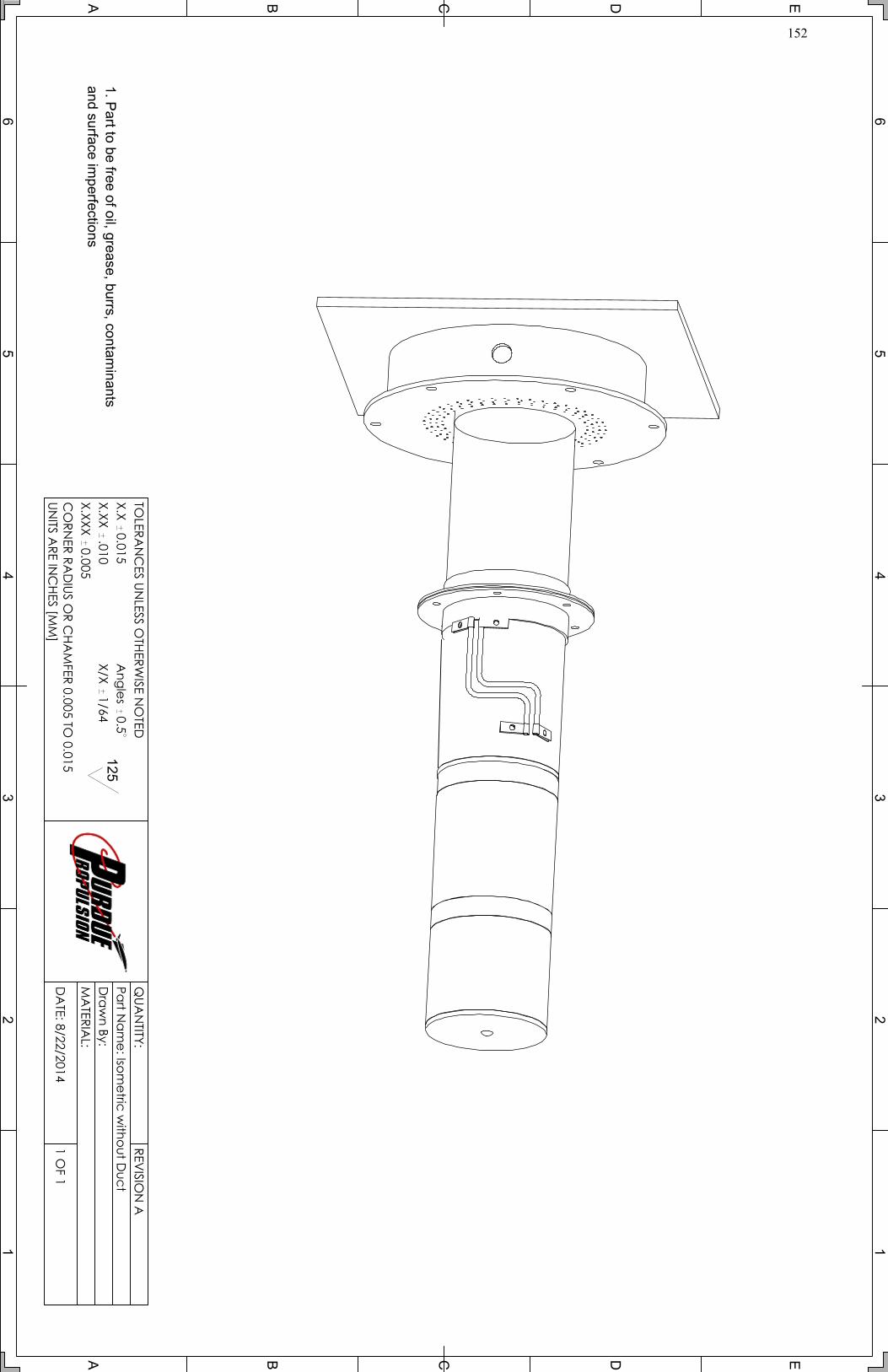
152

153

154

155

156

157

158

159

160

161

162

163
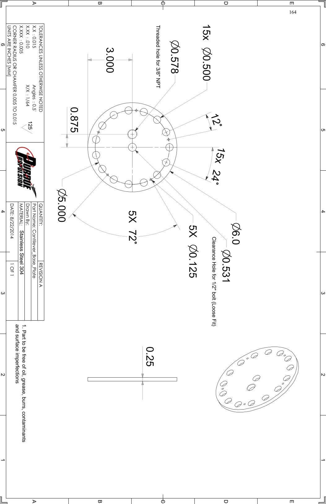
164

165

166

167

168

169

170

171

172

173

174

175

176

177

178

179

180

181

182

183

184

185

186