minimum wage and job mobility - banco central de … · minimum wage and job mobility nikita c...
TRANSCRIPT
BANCO CENTRAL DE RESERVA DEL PERÚ
Minimum Wage and Job Mobility
Nikita Céspedes Reynaga* y Alan Sánchez**
* Banco Central de Reserva del Perú y PUCP ** GRADE
DT. N° 2013-012 Serie de Documentos de Trabajo
Working Paper series Agosto 2013
Los puntos de vista expresados en este documento de trabajo corresponden a los autores y no reflejan
necesariamente la posición del Banco Central de Reserva del Perú.
The views expressed in this paper are those of the authors and do not reflect necessarily the position of the Central Reserve Bank of Peru.
Minimum Wage and Job Mobility∗
Nikita Cespedes Reynaga † Alan Sanchez ‡
(PUCP & BCRP) (GRADE)
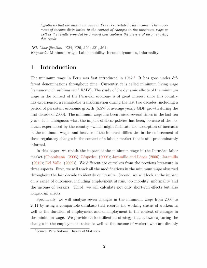
Resumen
Se estudia los efectos de cambios en el salario mınimo utilizando una base dedatos que registra 7 cambios consecutivos de este indicador (entre 2002 y 2011).Se estima que 1 millon de trabajadores tienen ingresos en la vecindad del salariomınimo. Los efectos sobre el empleo son decrecientes en terminos absolutossegun tamano de empresa: efecto moderado en empresas grandes y efectos may-ores en empresas pequenas. Finalmente, se sugiere que los cambios en el ingresoestan correlacionados con los cambios en el salario mınimo, este resultado sesustenta en los movimientos de la distribucion del ingreso ante cambios en elsalario mınimo y segun un modelo que captura los determinantes del ingreso.Los resultados son robustos a la alta rotacion del mercado laboral peruano, esdecir al considerar las transiciones empleo - empleo en los calculos.
Abstract
We study the effects of the minimum wage in over employment and income byconsidering a monthly database that captures seven minimum wage changes reg-istered between 2002 and 2011. We estimate that about 1 million workers havean income by main occupation in the neighbourhood of the minimum wage. Wefound that the minimum wage-income elasticity is statistically significant; theevidence also suggests that those who receive low incomes and those workingin small businesses are the most affected by increases in the minimum wage.Employment effects are monotonically decreasing in absolute terms by firm size:moderate in big firms and higher in small firms. Results are robust when as-sessing the job-to-job transitions. Finally, we present evidence that supports the
∗We thank Marcos Agurto, Juan Chacaltana, the editor, and numerous seminar participants forcomments that are incorporated throughout the paper. We are grateful to Jorge Luis Guzman Correafor excellent research assistance ant participants to the Research Seminar at the Central Bank of Peru.The views expressed in this paper are those of the authors and do not necessarily represent those ofthe Central Bank of Peru. All remaining errors are our own.†Pontificia Universidad Catolica del Peru and Central Bank of Peru. Email: [email protected]
[email protected]‡Grupo de Analisis para el Desarrollo. Email: [email protected]
1
hypothesis that the minimum wage in Peru is correlated with income. The move-ment of income distribution in the context of changes in the minimum wage aswell as the results provided by a model that captures the drivers of income justifythis result.
JEL Classification: E24, E26, J20, J21, J61.Keywords: Minimum wage, Labor mobility, Income dynamics, Informality.
1 Introduction
The minimum wage in Peru was first introduced in 1962.1 It has gone under dif-
ferent denominations throughout time. Currently, it is called minimum living wage
(remuneracion mınima vital, RMV). The study of the dynamic effects of the minimum
wage in the context of the Peruvian economy is of great interest since this country
has experienced a remarkable transformation during the last two decades, including a
period of persistent economic growth (5.5% of average yearly GDP growth during the
first decade of 2000). The minimum wage has been raised several times in the last ten
years. It is ambiguous what the impact of these policies has been, because of the bo-
nanza experienced by the country –which might facilitate the absorption of increases
in the minimum wage– and because of the inherent difficulties in the enforcement of
these regulatory changes in the context of a labour market that is still predominantly
informal.
In this paper, we revisit the impact of the minimum wage in the Peruvian labor
market (Chacaltana (2006); Cespedes (2006); Jaramillo and Lopez (2006); Jaramillo
(2012); Del Valle (2009)). We differentiate ourselves from the previous literature in
three aspects. First, we will track all the modifications in the minimum wage observed
throughout the last decade to identify our results. Second, we will look at the impact
on a range of outcomes, including employment status, job mobility, informality and
the income of workers. Third, we will calculate not only short-run effects but also
longer-run effects.
Specifically, we will analyze seven changes in the minimum wage from 2003 to
2011 by using a comparable database that records the working status of workers as
well as the duration of employment and unemployment in the context of changes in
the minimum wage. We provide an identification strategy that allows capturing the
changes in the employment status as well as the income of workers who are directly
1Source: Peru National Bureau of Statistics.
2
affected by changes in the minimum wages. This identification is based on the em-
ployment status of a panel of workers as well as their duration of employment and
unemployment.2 The methodology also provides some evidence of the indirect effects
of the minimum wage on both employment status and income. Summing up, by us-
ing a comparable database and also using our identification strategy, we are able to
perform a comprehensive evaluation of the various effects of the changes in minimum
wage over employment, informality, and the workers income.
We aim to provide answers to the following relevant questions: are changes in the
minimum wage important in the job market (in terms of employment and income)?
Has its importance changed throughout the last decade? How significant is the min-
imum wage in terms of job mobility? Does the minimum wage foster informality?
As we mentioned before, the available studies cover specific periods during a decade.
They also cover a relevant database to identify the effects of the minimum wage and
see if their importance has changed throughout the last decade of study.
According to the EPE (Encuesta Permanente de Empleo), around 20% of em-
ployed workers register job-to-job transitions towards a quarter, after having expe-
rienced short spells of unemployment or short spells of inactivity (out of the labour
market) within a quarter. Therefore, we identify the effects of the minimum wage on
employment status (or income) within a quarter when we take into account job mo-
bility. One interesting issue that is of interest in the context of the Peruvian economy
is related to the relationship between minimum wage and labour informality. Our
procedure is able to capture this: those who change jobs induced by the change in the
minimum wage can move from formal to informal job within a quarter. If this change
is statistically significant we will be able to suggest that the minimum wage fosters
informality in the labour market. In the same manner, we study the heterogeneous
effects in the changes in the minimum wage according to the size of the company and
different categories in the job market.
2In order to identify the effects of the minimum wage on employment we need to observe whetherthe employed workers are still employed after the change in the minimum wage. The databasethat captures this effect is the EPE (Encuesta Permanente de Empleo). This survey registers theemployment status of a group of workers twice, two monthly based observations with a 3-monthlag. By using the duration of employment we can identify if the workers do not experience job-to-jobtransitions. By using this database, once the minimum wage changes we can observe the employmentstatus of the workers after three months. This data covers only the Lima Metropolitan area, whichcan be a limitation since it represents only 30% of the population. The data that covers Peru isthe ENAHO (Encuesta Nacional de Hogares). However, this database only has yearly base panelobservations that may not be proper to capture the short term effects of minimum wage changes.The EPE allows us to capture both short term and long term effects of the minimum wage changes.
3
We estimate that about 1 million workers have an income by main occupation in
the neighbourhood of the minimum wage, with a greater participation in some sectors
and/or job categories (textiles, manufacturing, construction, trade, house workers,
etc.). We found that minimum wage changes have statistically significant effects on
employment and income. These results are robust after controlling for observable
micro heterogeneity, aggregate macro variables and seasonality of employment and
income. Our procedure also allows identifying the heterogeneous effect of minimum
wage changes according to firm size, employment status and income ranges.
This document is divided in 7 sections, including this introduction. Section 2
presents a brief discussion of the international evidence as well as of the evidence
available for Peru. Section 3 presents the data used in the formal estimation and the
motivation of the study. Section 4 shows the descriptive statistics. Section 5 illustrates
the effects of minimum wage over income and/or salaries. Section 6 is dedicated to
the study of the effects of the minimum wage on employment. Section 7 summarizes
the main results.
2 Literature review
The minimum wage literature is abundant worldwide. One of the first to study the
subject is Stigler (1946), who discusses the potential impact of increasing the post
war U.S. minimum wage on labor market outcomes as well as on welfare measures.
Brown,Gilroy and Kohen (1982) provides a survey of the early literature. Flinn (2011)
presents a synthesis of more recent contributions from a methodological perspective.
Among the most representative empirical studies are Card and Krueger (1994); Pereira
(2003); Bell (1997); Campolieti et al. (2005); Dinardo et al. (1996); Meyer and Wise
(1983a);Meyer and Wise (1983b); Brown,Gilroy and Kohen (1982); Neumark and
Wascher (1992); Eckstein and Wolpin (1990) and Van den Berg and Ridder (1998).
Prior to the 90s, most of the empirical evidence suggested that increases in the
minimum wage were harmful for employment. This is the expected outcome in a
competitive labor market. For the U.S., focusing on the segment of the population
that earns the minimum wage (teenagers and young adults) Brown,Gilroy and Kohen
(1982) present a synthesis of early studies based on time-series analysis. They conclude
that for workers around 16-19 years, a 10 percent increase in the minimum wage
tends to reduce employment by 1 to 3 percent (elasticity between -0.1 and -0.3). The
elasticity for workers around 20-24 years was found to be considerably smaller. Meyer
4
and Wise (1983a) reach a similar conclusion using micro-level data. In the early 90s,
this evidence was contested in a series of studies summarized in Card and Krueger
(1995) and best exemplified in the case study of the fast-food industry in New Jersey
and Pennsylvania (Card and Krueger, 1994). In this case, the authors were not able
to detect a negative effect of a marginal increase in minimum wages on employment.
Moreover, Katz and Krueger (1992) detected a positive effect on employment for this
industry. For similar evidence, see also Card (1992a).
A positive effect or a non-effect on employment is theoretically possible in the
context of firms with monopsony power. For instance, Van den Berg (2003) argues
that if firms have monopsony power and there are job search frictions, firms can pay
wages that are below the productivity level of the workers because it takes time for
them to find a better paying job. Under those circumstances, the adoption of a (or an
increase in the) minimum wage reduces the degree to which employers can exploit their
monopsony power without necessarily harming employment. Flinn (2011) reaches a
similar conclusion. While the evidence collected by Card and Krueger (1995) has
been influential and their results can be reconciled with theory, in a review of 102
studies published between 1990 and 2006, the so called “new minimum wage research
, Neumark and Wascher (2006) note that in about two thirds of the studies the
traditional result of a negative effect on employment is still found. For instance,
Neumark and Wascher (2006) exploit variation across states and over time in the
U.S. to find elasticities that corroborate the findings obtained by Brown,Gilroy and
Kohen (1982). Pereira (2003) uses micro-level data and a quasi-experimental setting
for Portugal. She finds that, for workers around 18-19 years, the elasticity is between -
0.2 and -0.4. Also exploiting a quasi-experimental setting, Orazem and Mattila (2002)
obtain elasticities between -0.06 and -0.12 for all workers and much larger (between
-0.31 and -0.85) for low-wage employees.
Overall, two aspects can be established from looking at the international literature.
First, most of the evidence seems to be consistent with the prediction that increases
in minimum wages lead to reductions in employment among the segment of the pop-
ulation that earns a salary close to the minimum wage. Second, there is awareness
that the specific effect of an increase in the minimum wage depends on the context.
For instance, the magnitude of the elasticity might vary according to the point in the
economic cycle that the country is facing or according to the proportion of the labor
force that earns an income close to the minimum wage.
The effects of the minimum wage in the Peruvian labor market have been analyzed
5
using a variety of empirical methods. A key aspect to bear in mind is that in Peru there
is a high concentration of workers whose earnings are located in the neighbourhood
of the minimum wage, so studies do not need to focus exclusively on the population
of teenager and young adults.3 Chacaltana (2006) provides a survey that includes
Cespedes (2006), Jaramillo and Lopez (2006) and Del Valle (2009). Cespedes uses
aggregated monthly employment data from the EPE and applies dynamic panel data
techniques to calculate the average impact of the minimum wage over employment ex-
ploiting the changes observed between 1997 and 2003. Jaramillo and Lopez (2006) use
individual-level data from the EPE to study the impact of the change in the minimum
wage observed in 2003. They estimate a linear probability model of employment sta-
tus conditional on having been employed three months ago. The estimation controls
for individual characteristics, firm characteristics, month fixed effects and quarterly
GDP growth. In the case of Del Valle, she uses the same database and implements a
difference-in-difference analysis of the changes observed in the minimum wage in 2003
and 2006, using the changes observed in year of no change as counterfactual.
Although the three studies mentioned above use different techniques, they reach
a qualitatively similar result: increases in the minimum wage lead to reductions in
average employment levels. Cespedes estimates an average elasticity of -0.13, whereas
Del Valle and Jaramillo and Lopez obtain a larger average elasticity (around -0.75 in
both cases). Both Del Valle and Jaramillo and Lopez allow in their estimation for het-
erogeneous effects according to the position of the individual in the wage distribution
prior to the policy change. Del Valle finds that the increase in the minimum wage
has a larger effect on those that earn below or around the minimum wage, whereas in
Jaramillo and Lopez (2006) the effect is larger on those who earn around or above the
minimum wage.
One limitation of Del Valle and Jaramillo and Lopez is that in both cases the
empirical identification relies on only one change in the minimum wage.4 However,
there have been several changes in the minimum wage in the last decade. Since there
have also been a persistent economic growth during the same time period, it is unclear
whether previous results are consistent. Another aspect to bear in mind is that these
studies look only at the short-run impact of the change in the minimum wage. Specif-
ically, they only consider as treated (affected by the policy change) those individuals
3Approximately 1 million workers may be exposed to minimum wage changes in Lima MetropolitanArea, in the sense that their income is in the neighbourhood of the minimum wage. Section 2.1characterizes the minimum wage workers in detail.
4Del Valle performs separate estimations for 2003 and 2006.
6
that are observed before and after a change in the minimum wage. However, it is
possible that other individuals are affected a few months after the change took place.
This is the case of people that have temporary contracts that cannot be fired in the
very short-run but that eventually might not have their contracts renewed.
In a recent study, Jaramillo (2012) updates Jaramillo and Lopez (2006) to simulta-
neously account for the changes observed in 2003, 2006, 2007 and 2010. Interestingly,
in this case the nature of the conclusions changes. According to the author, increases
in the minimum wage are found to increase employment for a segment of the informal
workers (those that earn slightly above the minimum wage) and to have no effect
on formal workers. Given that the sample is composed of workers that had a job the
previous quarter, what this suggests is that those that had an informal job in one quar-
ter were less likely to lose this employment status in the next quarter if an increase
in the minimum wage was observed. One possibility is that these results could be
telling something about the impact of changes in the minimum wage over job mobility
(transitions from the formal to the informal sector and vice versa).
The literature in Peru has also provided evidence of the effects of the changes
in minimum wage over earnings outcomes. Minimum wage changes can affect the
income distribution by directly affecting the income of formal workers and by indirectly
affecting the income of informal workers. This is the so called lighthouse effect, which
seems to be relevant in several studies worldwide. For Latin America, see Kristensen
and Cunningham (2006). For Peru, the relationship between income and minimum
wage was studied by Yamada and Bazan (1994), Jaramillo and Lopez (2006), Jaramillo
(2012), Cespedes (2006), among others. However, as in the previous case these
studies base their identification in one specific increase in the minimum wage observed
in 2003. The exceptions are Yamada and Bazan (1994) and Cespedes (2006)5, who
use a time-series econometric approach.
3 The data
The data comes from the EPE, which is done on a monthly basis by the Peru National
Bureau of Statistics (Instituto Nacional de Estadıstica e Informatica in Spanish, INEI).
The EPE is a survey specially conceived to trace labor market related aspects in Lima
Metropolitan Area. This geographic area comprehends 43 districts in the Province of
5Card and Kruger (1995) argued that time series analyses performed at the macro level may notcapture the distributional effects of maximum wage changes.
7
Lima and 6 districts in the Constitutional Province of Callao.
One of the main characteristic of this survey is that individuals who are interviewed
each month include a share of the sample (panel) who was interviewed three months
ago. The panel sample rotates partially each quarter in such a way that individuals
in the panel sample are interviewed twice in two consecutive quarters. In this paper,
we build a sequence of the quarterly unbalanced panel samples, from the first quarter
of 2003 to the first quarter of 2012. For the analysis we only look at individuals
that reported having a job in the previous interview. After missing values in some
demographic and labor market related variables, the panel sample built in this way
shows a total of 97,547 individuals, from which 82,552 (84.6%) were employed at the
time of the most recent interview. The rest are unemployed or inactive workers. For
the income analysis, in some instances we focus on those individuals for which an
income different from zero is observed in both periods. In this case the sample size
reduces to 76,282.
The level of inference of the quarter panel data is statistically significant, since
approximately 30% of the total sample is panel. As an example, the size of the quarter
sample in the EPE is of 4,800 households in 2011 from which 1,500 households had
already been interviewed in 2001. In this way, in 2011 the total quarter sample is of
approximately 18,500 people. Additionally, the size of quarter sample of the EPE has
being increasing throughout time. As a result, the estimates obtained from EPE are
currently more precise than at the beginning of the survey.
4 Descriptive statistics and the profile of workers
around minimum wage
Data from the EPE is used to characterize individuals with an income around the
minimum wage in Lima Metropolitan Area. All workers, whether formal or informal,
are included. In doing so, not only workers that earn the minimum wage but also
those that earn about the same level of monthly income by informal arrangement are
considered.
We provide a demographic profile as well as the type of economic activities in
which individuals that earn an income close to the minimum wage are involved. As
an operative definition, workers who earn a monthly income that is near the minimum
wage (+/- 100 Nuevos Soles) are considered as workers around the minimum wage
8
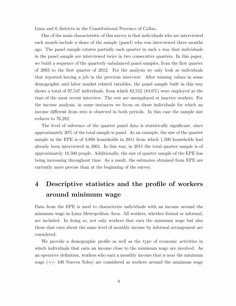
Group B, Table 1)6. We use data from a pooled sample of EPE surveys (from the first
quarter of 2007 to the fourth quarter of 2009) in order to increase sample size7.
It is found that approximately 18% of the employed population (around 1 million
people) earns an income within the minimum wage +/- 100 soles range (Table 1,
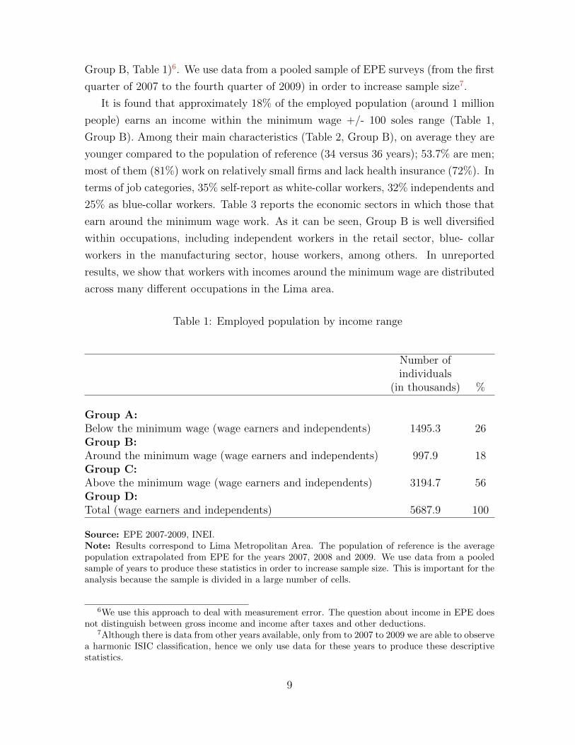
Group B). Among their main characteristics (Table 2, Group B), on average they are
younger compared to the population of reference (34 versus 36 years); 53.7% are men;
most of them (81%) work on relatively small firms and lack health insurance (72%). In
terms of job categories, 35% self-report as white-collar workers, 32% independents and
25% as blue-collar workers. Table 3 reports the economic sectors in which those that
earn around the minimum wage work. As it can be seen, Group B is well diversified
within occupations, including independent workers in the retail sector, blue- collar
workers in the manufacturing sector, house workers, among others. In unreported
results, we show that workers with incomes around the minimum wage are distributed
across many different occupations in the Lima area.
Table 1: Employed population by income range
Number ofindividuals
(in thousands) %
Group A:Below the minimum wage (wage earners and independents) 1495.3 26Group B:Around the minimum wage (wage earners and independents) 997.9 18Group C:Above the minimum wage (wage earners and independents) 3194.7 56Group D:Total (wage earners and independents) 5687.9 100
Source: EPE 2007-2009, INEI.Note: Results correspond to Lima Metropolitan Area. The population of reference is the averagepopulation extrapolated from EPE for the years 2007, 2008 and 2009. We use data from a pooledsample of years to produce these statistics in order to increase sample size. This is important for theanalysis because the sample is divided in a large number of cells.
6We use this approach to deal with measurement error. The question about income in EPE doesnot distinguish between gross income and income after taxes and other deductions.
7Although there is data from other years available, only from to 2007 to 2009 we are able to observea harmonic ISIC classification, hence we only use data for these years to produce these descriptivestatistics.
9
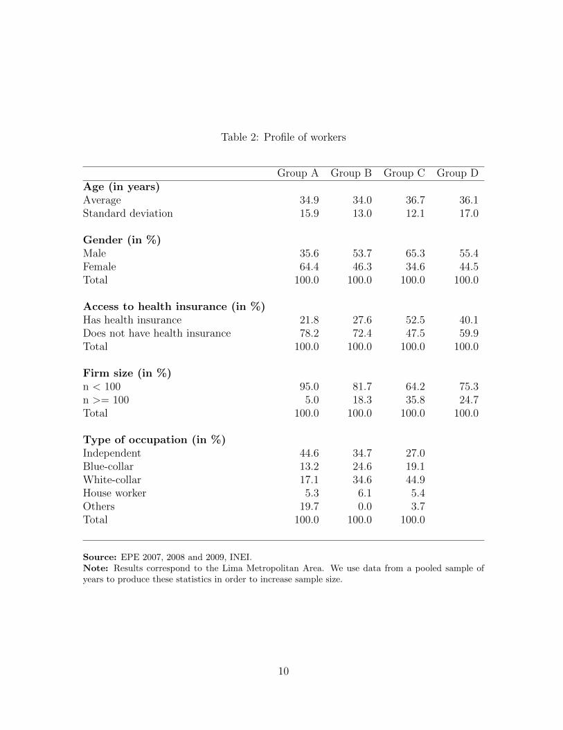
Table 2: Profile of workers
Group A Group B Group C Group DAge (in years)Average 34.9 34.0 36.7 36.1Standard deviation 15.9 13.0 12.1 17.0
Gender (in %)Male 35.6 53.7 65.3 55.4Female 64.4 46.3 34.6 44.5Total 100.0 100.0 100.0 100.0
Access to health insurance (in %)Has health insurance 21.8 27.6 52.5 40.1Does not have health insurance 78.2 72.4 47.5 59.9Total 100.0 100.0 100.0 100.0
Firm size (in %)n < 100 95.0 81.7 64.2 75.3n >= 100 5.0 18.3 35.8 24.7Total 100.0 100.0 100.0 100.0
Type of occupation (in %)Independent 44.6 34.7 27.0Blue-collar 13.2 24.6 19.1White-collar 17.1 34.6 44.9House worker 5.3 6.1 5.4Others 19.7 0.0 3.7Total 100.0 100.0 100.0
Source: EPE 2007, 2008 and 2009, INEI.Note: Results correspond to the Lima Metropolitan Area. We use data from a pooled sample ofyears to produce these statistics in order to increase sample size.
10
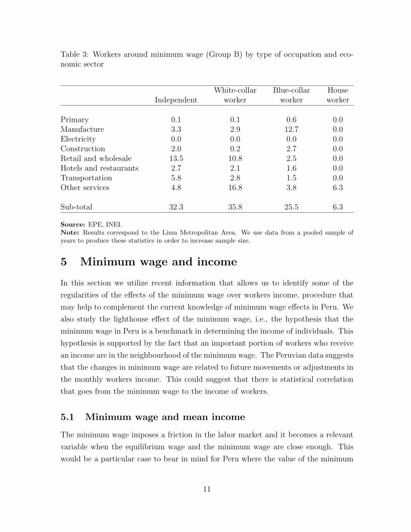
Table 3: Workers around minimum wage (Group B) by type of occupation and eco-nomic sector
White-collar Blue-collar HouseIndependent worker worker worker
Primary 0.1 0.1 0.6 0.0Manufacture 3.3 2.9 12.7 0.0Electricity 0.0 0.0 0.0 0.0Construction 2.0 0.2 2.7 0.0Retail and wholesale 13.5 10.8 2.5 0.0Hotels and restaurants 2.7 2.1 1.6 0.0Transportation 5.8 2.8 1.5 0.0Other services 4.8 16.8 3.8 6.3
Sub-total 32.3 35.8 25.5 6.3
Source: EPE, INEI.Note: Results correspond to the Lima Metropolitan Area. We use data from a pooled sample ofyears to produce these statistics in order to increase sample size.
5 Minimum wage and income
In this section we utilize recent information that allows us to identify some of the
regularities of the effects of the minimum wage over workers income, procedure that
may help to complement the current knowledge of minimum wage effects in Peru. We
also study the lighthouse effect of the minimum wage, i.e., the hypothesis that the
minimum wage in Peru is a benchmark in determining the income of individuals. This
hypothesis is supported by the fact that an important portion of workers who receive
an income are in the neighbourhood of the minimum wage. The Peruvian data suggests
that the changes in minimum wage are related to future movements or adjustments in
the monthly workers income. This could suggest that there is statistical correlation
that goes from the minimum wage to the income of workers.
5.1 Minimum wage and mean income
The minimum wage imposes a friction in the labor market and it becomes a relevant
variable when the equilibrium wage and the minimum wage are close enough. This
would be a particular case to bear in mind for Peru where the value of the minimum
11
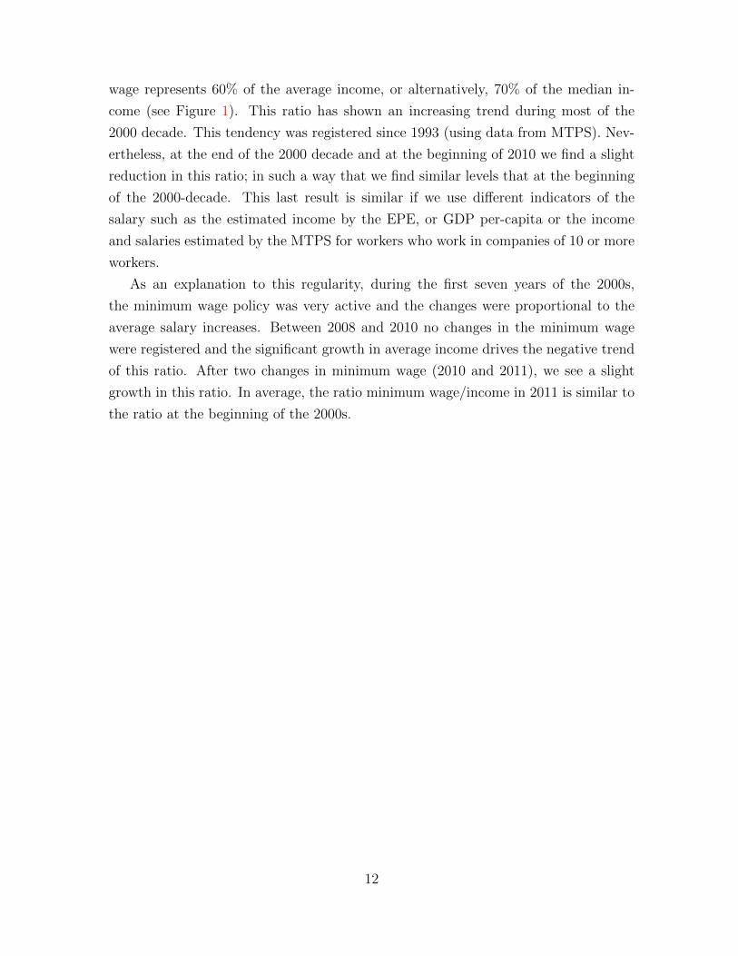
wage represents 60% of the average income, or alternatively, 70% of the median in-
come (see Figure 1). This ratio has shown an increasing trend during most of the
2000 decade. This tendency was registered since 1993 (using data from MTPS). Nev-
ertheless, at the end of the 2000 decade and at the beginning of 2010 we find a slight
reduction in this ratio; in such a way that we find similar levels that at the beginning
of the 2000-decade. This last result is similar if we use different indicators of the
salary such as the estimated income by the EPE, or GDP per-capita or the income
and salaries estimated by the MTPS for workers who work in companies of 10 or more
workers.
As an explanation to this regularity, during the first seven years of the 2000s,
the minimum wage policy was very active and the changes were proportional to the
average salary increases. Between 2008 and 2010 no changes in the minimum wage
were registered and the significant growth in average income drives the negative trend
of this ratio. After two changes in minimum wage (2010 and 2011), we see a slight
growth in this ratio. In average, the ratio minimum wage/income in 2011 is similar to
the ratio at the beginning of the 2000s.
12
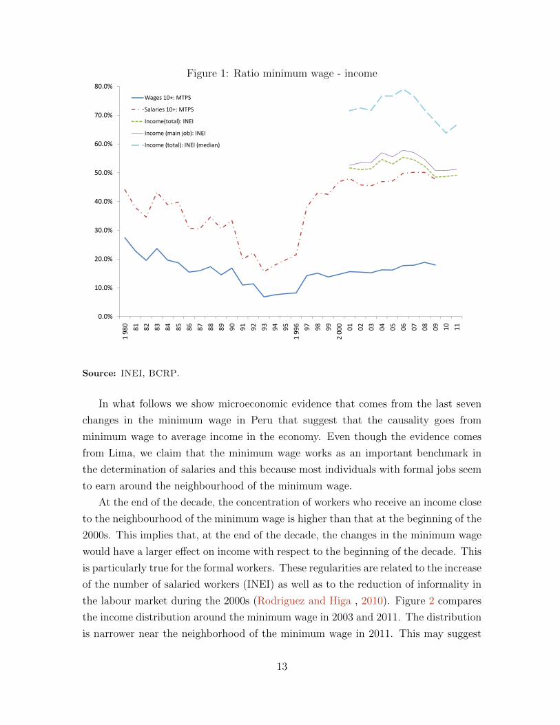
Figure 1: Ratio minimum wage - income
40.0%
50.0%
60.0%
70.0%
80.0%
Wages 10+: MTPS
Salaries 10+: MTPS
Income(total): INEI
Income (main job): INEI
Income (total): INEI (median)
0.0%
10.0%
20.0%
30.0%
40.0%
1 9
80
81
82
83
84
85
86
87
88
89
90
91
92
93
94
95
1 9
96
97
98
99
2 0
00
01
02
03
04
05
06
07
08
09
10
11
1 9
80
81
82
83
84
85
86
87
88
89
90
91
92
93
94
95
1 9
96
97
98
99
2 0
00
01
02
03
04
05
06
07
08
09
10
11
Source: INEI, BCRP.
In what follows we show microeconomic evidence that comes from the last seven
changes in the minimum wage in Peru that suggest that the causality goes from
minimum wage to average income in the economy. Even though the evidence comes
from Lima, we claim that the minimum wage works as an important benchmark in
the determination of salaries and this because most individuals with formal jobs seem
to earn around the neighbourhood of the minimum wage.
At the end of the decade, the concentration of workers who receive an income close
to the neighbourhood of the minimum wage is higher than that at the beginning of the
2000s. This implies that, at the end of the decade, the changes in the minimum wage
would have a larger effect on income with respect to the beginning of the decade. This
is particularly true for the formal workers. These regularities are related to the increase
of the number of salaried workers (INEI) as well as to the reduction of informality in
the labour market during the 2000s (Rodriguez and Higa , 2010). Figure 2 compares
the income distribution around the minimum wage in 2003 and 2011. The distribution
is narrower near the neighborhood of the minimum wage in 2011. This may suggest
13
that there is a tendency to receive salaries closer to the minimum wage.
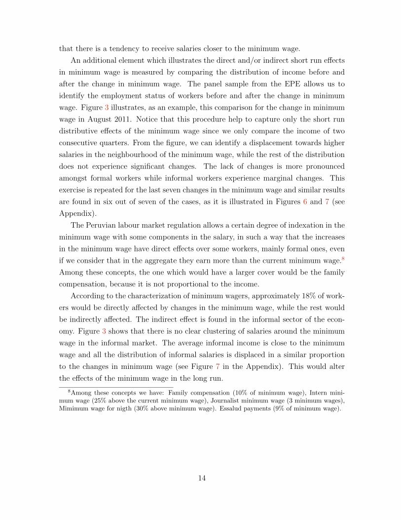
An additional element which illustrates the direct and/or indirect short run effects
in minimum wage is measured by comparing the distribution of income before and
after the change in minimum wage. The panel sample from the EPE allows us to
identify the employment status of workers before and after the change in minimum
wage. Figure 3 illustrates, as an example, this comparison for the change in minimum
wage in August 2011. Notice that this procedure help to capture only the short run
distributive effects of the minimum wage since we only compare the income of two
consecutive quarters. From the figure, we can identify a displacement towards higher
salaries in the neighbourhood of the minimum wage, while the rest of the distribution
does not experience significant changes. The lack of changes is more pronounced
amongst formal workers while informal workers experience marginal changes. This
exercise is repeated for the last seven changes in the minimum wage and similar results
are found in six out of seven of the cases, as it is illustrated in Figures 6 and 7 (see
Appendix).
The Peruvian labour market regulation allows a certain degree of indexation in the
minimum wage with some components in the salary, in such a way that the increases
in the minimum wage have direct effects over some workers, mainly formal ones, even
if we consider that in the aggregate they earn more than the current minimum wage.8
Among these concepts, the one which would have a larger cover would be the family
compensation, because it is not proportional to the income.
According to the characterization of minimum wagers, approximately 18% of work-
ers would be directly affected by changes in the minimum wage, while the rest would
be indirectly affected. The indirect effect is found in the informal sector of the econ-
omy. Figure 3 shows that there is no clear clustering of salaries around the minimum
wage in the informal market. The average informal income is close to the minimum
wage and all the distribution of informal salaries is displaced in a similar proportion
to the changes in minimum wage (see Figure 7 in the Appendix). This would alter
the effects of the minimum wage in the long run.
8Among these concepts we have: Family compensation (10% of minimum wage), Intern mini-mum wage (25% above the current minimum wage), Journalist minimum wage (3 minimum wages),Mimimum wage for nigth (30% above minimum wage). Essalud payments (9% of minimum wage).
14
Figure 2: Income from main job, frequency 2003 and 2011b
0.2
.4.6
.8
4 6 8 10log(income)
2003 2011
All
0.2
.4.6
.8
4 6 8 10log(income)
2003 2011
Formal (Blue collar and White collar)
Note: Income frequencies (EPE, Lima Metropolitan area). Vertical line represents the minimum
wage in 2003 or 2011, respectively. Kernel Epanechnikov function.
Figure 3: Income from main job, Frequencies 2011b
0.2
.4.6
.8
4 6 8 10log(income)
Before After
Formal (Blue collar and White collar)
0.2
.4.6
.8
4 6 8 10log(income)
Before After
Informal
Note: Frequencies before and after the current minimum wage rise (EPE, Lima Metropolitan area).
Vertical line represents the minimum wage in 2011. Kernel Epanechnikov function.
15
5.2 Minimum wage and income: a formal model
In order to more robustly assess the relationship between minimum wage and income,
an equation of income determinants at the level of the workers is estimated. This
equation includes several controls to capture demographic characteristics, income het-
erogeneity of workers, income seasonality and the business cycle. We take advantage
that in the EPE a share of the individuals is interviewed twice to condition the analysis
on some characteristics from the first interview. The specification is as follows,
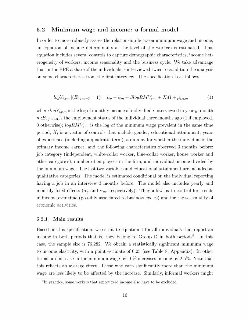
logYi,y,m|(Ei,y,m−3 = 1) = αy + αm + βlogRMVy,m +XiΩ + µi,y,m (1)
where logYi,y,m is the log of monthly income of individual i interviewed in year y, month
m;Ei,y,m−3 is the employment status of the individual three months ago (1 if employed,
0 otherwise); logRMVy,m is the log of the minimum wage prevalent in the same time
period; Xi is a vector of controls that include gender, educational attainment, years
of experience (including a quadratic term), a dummy for whether the individual is the
primary income earner, and the following characteristics observed 3 months before:
job category (independent, white-collar worker, blue-collar worker, house worker and
other categories), number of employees in the firm, and individual income divided by
the minimum wage. The last two variables and educational attainment are included as
qualitative categories. The model is estimated conditional on the individual reporting
having a job in an interview 3 months before. The model also includes yearly and
monthly fixed effects (αy and αm, respectively). They allow us to control for trends
in income over time (possibly associated to business cycles) and for the seasonality of
economic activities.
5.2.1 Main results
Based on this specification, we estimate equation 1 for all individuals that report an
income in both periods that is, they belong to Group D in both periods9. In this
case, the sample size is 76,282. We obtain a statistically significant minimum wage
to income elasticity, with a point estimate of 0.25 (see Table 8, Appendix). In other
terms, an increase in the minimum wage by 10% increases income by 2.5%. Note that
this reflects an average effect. Those who earn significantly more than the minimum
wage are less likely to be affected by the increase. Similarly, informal workers might
9In practice, some workers that report zero income also have to be excluded.
16
not benefit or might benefit only partially from the increase.
6 Minimum wage and employment
In this section we study the relationship between minimum wage and employment. As
mentioned in Section 2, the general conclusion for the Peruvian case is that the mini-
mum wage has a negative effect on employment. In order to study this relationship, we
use the information provided by the EPE, which allows us to track labor transitions in
the context of changes in the minimum wage. Our approach allows us to capture not
only the transitions in employment towards unemployment and/or towards inactivity
but also toward another job (job-to-job transitions). We use the job duration data to
estimate the short term job-to-job transitions in the context of a changing minimum
wage.
The previous point is particularly important in Peru because the aggregate statis-
tics about employment could not capture adequately the short term job mobility which
may be driven by changes in the minimum wage. The employment status of the same
worker is observed with a three months lag. These two observations of the same worker
does not allow us to identify if this worker has experienced a short spell of unemploy-
ment. In a context of changes in the minimum wage, it is possible to observe the same
individual working before and after the change in minimum wage and if we do not
control for this short term unemployment spell we cannot observe the job loss due to
rise of the minimum wage. Given that the unemployment duration in Peru is short,
between 12-15 weeks (Chacaltana (2000); Diaz and Maruyama (2000)10, then the
quarterly separation between two consecutive employment status does not allow us to
identify the likely destruction (or not) of jobs due to a change in minimum wage. We
need to estimate job-to-job transitions in order to identify the role of the minimum
wage in employment transitions.
The importance of job-to-job transitions in the identification of the short run effects
of the minimum wage on employment is illustrated in Figure 4, which considers the
impact of the increase in the minimum wage in 2011. The second graph of this figure
shows the job-to-other categories transitions (unemployment, inactivity or other jobs)
across the income range.11 We present the transitions of the treatment group, with
10The duration of unemployment estimated from EPE has similar values with a decreasing trendduring most of the decade, Cespedes et al. (2013).
11The income range is defined according to the income prevalent prior to the change in the minimumwage.
17
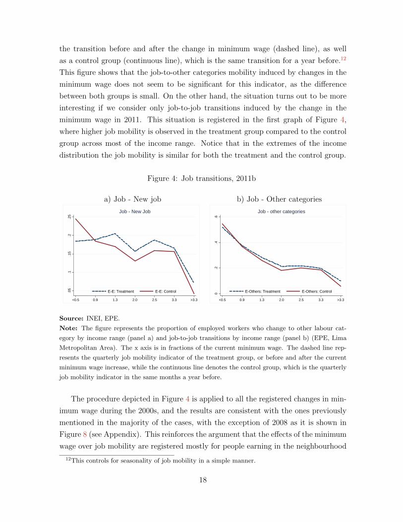
the transition before and after the change in minimum wage (dashed line), as well
as a control group (continuous line), which is the same transition for a year before.12
This figure shows that the job-to-other categories mobility induced by changes in the
minimum wage does not seem to be significant for this indicator, as the difference
between both groups is small. On the other hand, the situation turns out to be more
interesting if we consider only job-to-job transitions induced by the change in the
minimum wage in 2011. This situation is registered in the first graph of Figure 4,
where higher job mobility is observed in the treatment group compared to the control
group across most of the income range. Notice that in the extremes of the income
distribution the job mobility is similar for both the treatment and the control group.
Figure 4: Job transitions, 2011b
a) Job - New job b) Job - Other categories
.05
.1.1
5.2
.25
<0.5 0.9 1.3 2.0 2.5 3.3 >3.3R I
E-E: Treatment E-E: Control
Job - New Job0
.2.4
.6
<0.5 0.9 1.3 2.0 2.5 3.3 >3.3R I
E-Others: Treatment E-Others: Control
Job - other categories
Source: INEI, EPE.
Note: The figure represents the proportion of employed workers who change to other labour cat-
egory by income range (panel a) and job-to-job transitions by income range (panel b) (EPE, Lima
Metropolitan Area). The x axis is in fractions of the current minimum wage. The dashed line rep-
resents the quarterly job mobility indicator of the treatment group, or before and after the current
minimum wage increase, while the continuous line denotes the control group, which is the quarterly
job mobility indicator in the same months a year before.
The procedure depicted in Figure 4 is applied to all the registered changes in min-
imum wage during the 2000s, and the results are consistent with the ones previously
mentioned in the majority of the cases, with the exception of 2008 as it is shown in
Figure 8 (see Appendix). This reinforces the argument that the effects of the minimum
wage over job mobility are registered mostly for people earning in the neighbourhood
12This controls for seasonality of job mobility in a simple manner.
18
of the current minimum wage.
We can extend this analysis to other indicators of transition in the labor market.
Consider, for instance, the unemployment to employment transitions. In this case,
an increase in the minimum wage may reduce the job creation for those workers that
expect to receive an income close to the minimum wage. We do not find support
for this hypothesis. As shown in Figure 12 (Appendix), we cannot identify a strong
movement in the neighbourhood of the minimum wage. In a similar fashion, figures
10, 11 and 13 (Appendix) show that minimum wage changes may not have a clear
effect in other employment transitions.
6.1 Minimum wage and employment: a formal model
Using the previous results as a motivation, we estimate a discrete response probit
model to capture the relationship between the minimum wage and employment status.
We consider the following functional form
Pr(Ei,y,m = 1|Ei,y,m−3 = 1) = G(αy + αm . . . (2)
+ρRMVy,m +XiΩ + µi,y,m)
where Pr(Ei,y,m) takes the value of 1 if individual i is employed in month m of year
y. G(.) is the cumulative distribution function of the standard normal distribution
.RMVy,m is the prevalent minimum wage in the same time period; Xi is a vector
that contains the same control variables used in equation 2. As in Section 5.2, the
model also includes yearly and monthly fixed effects (αy and αm, respectively) and is
estimated conditional on the individual having had a job as reported in an interview
3 months before. The result of interest is the elasticity of the minimum wage to the
probability of being employed, conditional on having a job 3 months before.13
6.1.1 Main results
Based on this specification, equation 2 is estimated for all individuals that fulfil the
condition of having a job three months ago. That is, they belong to Group D in
13In this set of estimations the non-employed status includes the unemployed as well as thosethat self-report as inactive (out of the economically active population). We consider both categoriesbecause we are already conditioning the analysis to having had a job three months ago, which alreadyexcludes the structural proportion of the population that is not actively looking for a job.
19
the first interview. Sample size is 97,547. In Table 9, column 1 (see Appendix), the
coefficients associated to the model described in Equation 2 are presented using data
from EPE (Lima Metropolitan Area). These results imply a negative, statistically
significant relationship between minimum wage and employment. In column 2, the
model allows for differential effects according to job category: independent, blue-collar,
white-collar, house workers and other categories. In this case, results suggest that the
relationship initially found holds also for independent workers.
To have a better sense of the results, elasticities derived from these two models
are reported in Table 4. The minimum wage - employment elasticity for the average
individual in the sample is -0,25; a 10% increase in the minimum wage reduces em-
ployment by 2.5%. Highest values of the elasticity are observed for those self-reported
as blue-collar and white-collar workers, whereas those self-reported as independent
workers are the less affected by changes in the minimum wage regulation.
The average impact of the minimum wage on employment is likely to mask some
heterogeneity. A priori those with a formal job are more likely to be affected because
formal firms are required by law to fulfil minimum wage policies. In the same way,
people who earn the minimum wage, or around it, are likely to be the target of
job cuts. To take into account these possibilities, we re-estimate our employment
model allowing for heterogeneous minimum wage effects according to the following
characteristics three months before: (a) whether or not the individual had health
insurance in his job (a proxy of formal employment); (b) position of the individual in
the income / minimum wage ratio distribution; and, (c) size of the firm. Results for
(b) and (c) are shown graphically in Figure 5. Full results are reported in Table 10
(Appendix B).14 We observe that workers without health insurance, with lower income
levels and working on small firms are the most affected by increases in minimum wage.
We find that not only those that earned around the minimum wage are affected, but
also those that earned less than the minimum wage are affected. In fact, results suggest
that those who earn less than the minimum wage are the most affected. In contrast,
those that earn more than four times the minimum wage are not affected.
To check whether a similar relationship between minimum wage and employment
can be found at the national level, we use data from the Peruvian National House-
hold Survey (Encuesta Nacional de Hogares, ENAHO) to produce estimates of this
elasticity distinguishing between rural areas, urban areas (excluding Lima) and Lima
Metropolitan Area. For this exercise we cannot replicate the model specified in equa-
14See coefficients of the Probit model in Table 11 (Appendix).
20
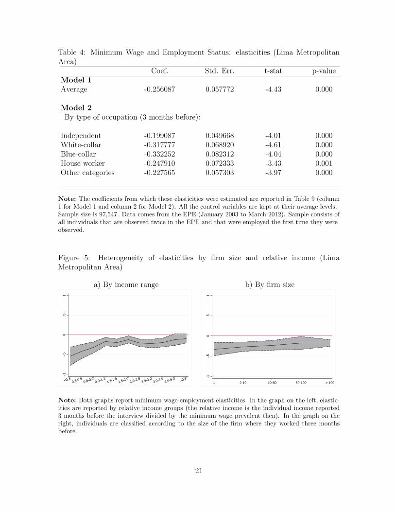
Table 4: Minimum Wage and Employment Status: elasticities (Lima MetropolitanArea)
Coef. Std. Err. t-stat p-valueModel 1Average -0.256087 0.057772 -4.43 0.000
Model 2By type of occupation (3 months before):
Independent -0.199087 0.049668 -4.01 0.000White-collar -0.317777 0.068920 -4.61 0.000Blue-collar -0.332252 0.082312 -4.04 0.000House worker -0.247910 0.072333 -3.43 0.001Other categories -0.227565 0.057303 -3.97 0.000
Note: The coefficients from which these elasticities were estimated are reported in Table 9 (column1 for Model 1 and column 2 for Model 2). All the control variables are kept at their average levels.Sample size is 97,547. Data comes from the EPE (January 2003 to March 2012). Sample consists ofall individuals that are observed twice in the EPE and that were employed the first time they wereobserved.
Figure 5: Heterogeneity of elasticities by firm size and relative income (LimaMetropolitan Area)
a) By income range b) By firm size
-1-.
50
.51
<0.30.3-0.6
0.6-0.90.9-1.2
1.2-1.51.5-2.0
2.0-2.52.5-3.0
3.0-4.04.0-5.0 >0.5
-1-.
50
.51
1 2-10 10-50 50-100 > 100
Note: Both graphs report minimum wage-employment elasticities. In the graph on the left, elastic-ities are reported by relative income groups (the relative income is the individual income reported3 months before the interview divided by the minimum wage prevalent then). In the graph on theright, individuals are classified according to the size of the firm where they worked three monthsbefore.
21
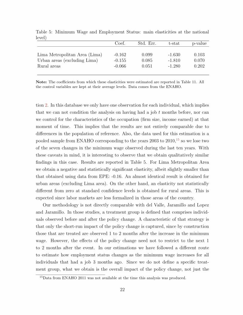
Table 5: Minimum Wage and Employment Status: main elasticities at the nationallevel)
Coef. Std. Err. t-stat p-value
Lima Metropolitan Area (Lima) -0.162 0.099 -1.630 0.103Urban areas (excluding Lima) -0.155 0.085 -1.810 0.070Rural areas -0.066 0.051 -1.280 0.202
Note: The coefficients from which these elasticities were estimated are reported in Table 11. Allthe control variables are kept at their average levels. Data comes from the ENAHO.
tion 2. In this database we only have one observation for each individual, which implies
that we can not condition the analysis on having had a job t months before, nor can
we control for the characteristics of the occupation (firm size, income earned) at that
moment of time. This implies that the results are not entirely comparable due to
differences in the population of reference. Also, the data used for this estimation is a
pooled sample from ENAHO corresponding to the years 2003 to 2010,15 so we lose two
of the seven changes in the minimum wage observed during the last ten years. With
these caveats in mind, it is interesting to observe that we obtain qualitatively similar
findings in this case. Results are reported in Table 5. For Lima Metropolitan Area
we obtain a negative and statistically significant elasticity, albeit slightly smaller than
that obtained using data from EPE: -0.16. An almost identical result is obtained for
urban areas (excluding Lima area). On the other hand, an elasticity not statistically
different from zero at standard confidence levels is obtained for rural areas. This is
expected since labor markets are less formalized in those areas of the country.
Our methodology is not directly comparable with del Valle, Jaramillo and Lopez
and Jaramillo. In those studies, a treatment group is defined that comprises individ-
uals observed before and after the policy change. A characteristic of that strategy is
that only the short-run impact of the policy change is captured, since by construction
those that are treated are observed 1 to 2 months after the increase in the minimum
wage. However, the effects of the policy change need not to restrict to the next 1
to 2 months after the event. In our estimations we have followed a different route
to estimate how employment status changes as the minimum wage increases for all
individuals that had a job 3 months ago. Since we do not define a specific treat-
ment group, what we obtain is the overall impact of the policy change, not just the
15Data from ENAHO 2011 was not available at the time this analysis was produced.
22
short-run impact. This has consequences for the interpretation of the results. If jobs
that are destroyed by the increase in the minimum wage can be recovered relatively
quickly, the short-run elasticity will be larger than our estimates (in absolute terms).
Conversely, if the increase in the minimum wage makes a worker more likely to lose
his job a few months after the policy change, the short-term elasticity will be smaller
than our estimates (in absolute terms).
To check whether the short-run elasticity is smaller or larger than our overall
elasticity, in Table 8 we re-estimate our main specification defining a treatment variable
that takes the value of 1 for those individuals that are observed before and after a
change in the minimum wage and 0 otherwise. When doing this we obtain an average
elasticity of -0.13. The point estimate is not statistically different from zero. When
we calculate the elasticity allowing for heterogeneity by type of occupation an average
elasticity of -0.46 is obtained for white-collar workers, a result that is statistically
significant. For the other groups (independent workers, blue-collar workers and house
workers) the elasticities obtained are not statistically significant. This differs from our
previous results in which we obtained a larger average elasticity as well as elasticities
that were statistically significant for all the sub-groups by type of occupation. The
difference between the two sets of results suggests that an increase in the minimum
wage has wider implications on employment status that are not necessarily apparent
in the short-run.
6.2 Minimum wage and labour mobility
A change in the minimum wage might affect employment in ways that are not captured
by the previous definition (1 if employed at the time of the interview, 0 otherwise,
conditional on having had a job three months before). People who lose jobs might
quickly find new ones (e.g., within less than a month). Depending on the exact timing
of the household survey interviews and the changes in the minimum wage, it is possible
that people who lost their jobs because of the increase in the minimum wage might
have found a new one by the time of the interview. If this is the case, previous results
would be a lower bound of the true minimum wage - employment elasticity. To take
into account this possibility, we estimate the change in the probability of retaining the
same job compared to the alternative of having a new job.16 Because this is a selected
16In the dataset, it is possible to know for how long the individual has been in his current job andwhether he had a job 3 months ago. If he had a job 3 months ago but has been less than 3 monthsin his current position, we assume there was a job transition.
23
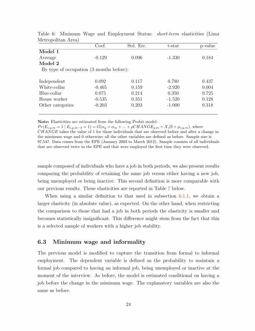
Table 6: Minimum Wage and Employment Status: short-term elasticities (LimaMetropolitan Area)
Coef. Std. Err. t-stat p-valueModel 1Average -0.129 0.096 -1.330 0.184Model 2By type of occupation (3 months before):
Independent 0.092 0.117 0.780 0.437White-collar -0.465 0.159 -2.920 0.004Blue-collar 0.075 0.214 0.350 0.725House worker -0.535 0.351 -1.520 0.128Other categories -0.203 0.203 -1.000 0.318
Note: Elasticities are estimated from the following Probit model:Pr(Ei,y,m = 1 | Ei,y,m−3 = 1) = G(αy + αm + ...+ ρCHANGEy,m +XiΩ + µi,y,m), whereCHANGE takes the value of 1 for those individuals that are observed before and after a change inthe minimum wage and 0 otherwise; all the other variables are defined as before. Sample size is97,547. Data comes from the EPE (January 2003 to March 2012). Sample consists of all individualsthat are observed twice in the EPE and that were employed the first time they were observed.
sample composed of individuals who have a job in both periods, we also present results
comparing the probability of retaining the same job versus either having a new job,
being unemployed or being inactive. This second definition is more comparable with
our previous results. These elasticities are reported in Table 7 below.
When using a similar definition to that used in subsection 6.1.1, we obtain a
larger elasticity (in absolute value), as expected. On the other hand, when restricting
the comparison to those that had a job in both periods the elasticity is smaller and
becomes statistically insignificant. This difference might stem from the fact that this
is a selected sample of workers with a higher job stability.
6.3 Minimum wage and informality
The previous model is modified to capture the transition from formal to informal
employment. The dependent variable is defined as the probability to maintain a
formal job compared to having an informal job, being unemployed or inactive at the
moment of the interview. As before, the model is estimated conditional on having a
job before the change in the minimum wage. The explanatory variables are also the
same as before.
24
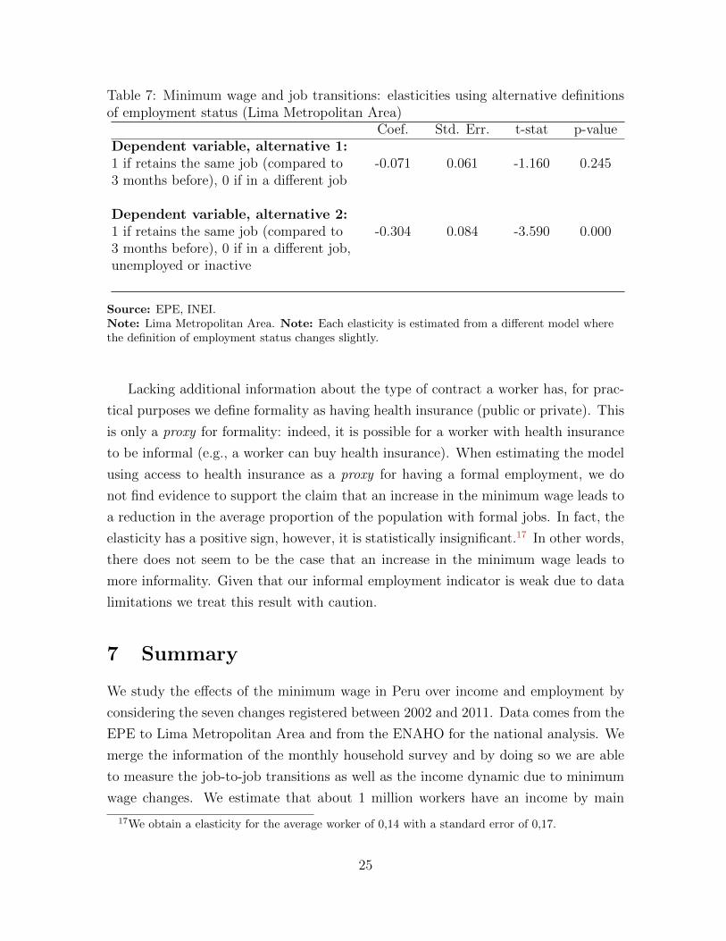
Table 7: Minimum wage and job transitions: elasticities using alternative definitionsof employment status (Lima Metropolitan Area)
Coef. Std. Err. t-stat p-valueDependent variable, alternative 1:1 if retains the same job (compared to -0.071 0.061 -1.160 0.2453 months before), 0 if in a different job
Dependent variable, alternative 2:1 if retains the same job (compared to -0.304 0.084 -3.590 0.0003 months before), 0 if in a different job,unemployed or inactive
Source: EPE, INEI.Note: Lima Metropolitan Area. Note: Each elasticity is estimated from a different model wherethe definition of employment status changes slightly.
Lacking additional information about the type of contract a worker has, for prac-
tical purposes we define formality as having health insurance (public or private). This
is only a proxy for formality: indeed, it is possible for a worker with health insurance
to be informal (e.g., a worker can buy health insurance). When estimating the model
using access to health insurance as a proxy for having a formal employment, we do
not find evidence to support the claim that an increase in the minimum wage leads to
a reduction in the average proportion of the population with formal jobs. In fact, the
elasticity has a positive sign, however, it is statistically insignificant.17 In other words,
there does not seem to be the case that an increase in the minimum wage leads to
more informality. Given that our informal employment indicator is weak due to data
limitations we treat this result with caution.
7 Summary
We study the effects of the minimum wage in Peru over income and employment by
considering the seven changes registered between 2002 and 2011. Data comes from the
EPE to Lima Metropolitan Area and from the ENAHO for the national analysis. We
merge the information of the monthly household survey and by doing so we are able
to measure the job-to-job transitions as well as the income dynamic due to minimum
wage changes. We estimate that about 1 million workers have an income by main
17We obtain a elasticity for the average worker of 0,14 with a standard error of 0,17.
25
occupation in the neighbourhood of the minimum wage, with a greater participation
in some sectors and / or job categories (textiles, manufacturing, construction, trade,
house workers, etc.).
By using a model that explains the probability of being employed we estimate
statistically significant minimum wage-employment elasticity for the average worker.
Although on average both formal and informal workers are affected, those seemingly
engaged in formal activities are hit harder. The evidence also suggests that those
who receive low incomes and those working in small businesses are the most affected
by increases in the minimum wage. Effects are monotonically decreasing in absolute
terms by firm size, this is, and the effects of minimum wage changes are moderate in
big firms and higher in small firms.
The minimum wage -employment elasticity is larger in absolute value (mostly
negative) when assessing the probability that the individual is working in the same job
in both periods. This suggests that part of the effect of the minimum wage changes
on employment is cleared due to the ability of individuals to quickly re-insert in a
dynamic labour market (recall the persistent economic growth during this decade).
By estimating the model considering informality, we find that the increases in the
minimum wage do not appear to reduce the probability of being formally employed.
However, this results needs to be revisited with proper data, given that our informal
employment indicator is weak due to data limitations.
Finally, we present evidence for the hypothesis that the minimum wage in Peru is
a benchmark in determining the income of individuals (lighthouse effect). Causality
tests, movement of the income distribution in the context of change of changes in
the minimum wage, and the results provided by a model that captures the drivers of
income justify these results.
26
References
Bell, L. (1997), “The impact of minimum wages in Mexico and Colombia”, Journal of Labour
Economics 15(S3), S102-S135.
Brown, C., C. Gilroy and A. Kohen (1983), “Time-Series Evidence of the Effect of the
Minimum Wage on Youth Employment and Unemployment”, Journal of Human Resources
18(1), 3-31.
Brown, C., C. Gilroy and A. Kohen (1983), “The Effect of the Minimum Wage on Employ-
ment and Unemployment”, Journal of Economic Literature 10 487-528.
Campolieti, M., T. Fang and M. Gunderson (2005), “Minimum wages impacts on youth
employment transitions”, Canadian Journal of Economics 38(1), 81-104.
Card, D. (1992), “Using Regional Variation in Wages to Measure the Effects of the Federal
Minimum Wage”, Industrial and Labor Relations Review 84(4), 46(1), 22-37.
Card, D. (1992), “Minimum Wages Reduce Employment? A Case Study of California, 1987-
89”, Industrial and Labor Relations Review 84(4), 46(1), 38-54.
Card, D. and A. Krueger (1994), “Minimum wages and employment: a case study of the
fast-food industry in New Jersey and Pennsylvania”, American Economic Review 84(4),
772-793.
Card, D. and A. Krueger (1995), “Myth and measurement: The new economics of the
minimum wage”, Princeton University Press.
Cespedes, N. (2006), “ Efectos del salario mınimo en el mercado laboral peruano”, Revista
Estudios Economicos, Banco Central de Reserva del Peru, 13(1).
Cespedes, N., B. Belapatino and A. Gutierrez (2013), “ Duracion del desempleo en el Peru”,
Mimeo.
Chacaltana, J. (2000), “Un analisis dinamico del desempleo en el Peru”, Fondo de Investi-
gaciones del Programa MECOVI-Peru. Lima. INEI. 2000.
Chacaltana, J. (2006), “Que hacemos con el salario mınimo?”, Economıa y Sociedad 60,
CIES, junio 2006.
Del Valle, M. (2009), “Impacto del ajuste de la Remuneracion Mınima Vital sobre el empleo
y la informalidad”, Revista Estudios Economicos, Banco Central de Reserva del Peru,
issue 16, pages 83-102.
27
Dıaz, J. and E. Maruyama (2000), “La dinamica del desempleo urbano en el Peru: tiempo
de busqueda y rotacion laboral”, Lima. GRADE. 2000.
Dinardo, J., N. Fortin and T. Lemieux (1996), “Labour market institutions and the distribu-
tion of wages, 1973-1992: a semi-parametric approach”, Econometrica 64(5), 1001-1044.
Eckstein, Z. and K. Wolpin (1990), “Estimating a Market Equilibrium Search Model from
Panel Data on Individuals”, Econometrica 58(4), 783-808.
Flinn, C. (2011), The Minimum Wage and Labor Market Outcomes, The MIT Press.
Jaramillo, M. (2012), “Ajustes del mercado laboral peruano ante cambios en el salario
mınimo: la experiencia de la decada de 2000”, Documentos de Trabajo, Grupo de Analisis
para el Desarrollo (GRADE).
Jaramillo, M. and K. Lopez (2006), “ Como se ajusta el mercado de trabajo ante cambios
en el salario mınimo en el Peru? Una evaluacion de la experiencia de la ultima decada”,
Documentos de Trabajo 50, Grupo de Analisis para el Desarrollo (GRADE).
Katz, L. and A. Krueger (1992), “The Effect of the Minimum Wage on the Fast Food
Industry”, Industrial and Labor Relations Review 46(1), 6-21.
Kristensen, N. and W. Cunningham (1992), “Do minimum wages in Latin America and
the Caribbean Matter? Evidence from 19 Countries”, Working Paper 3870, World Bank
Policy Research Series.
Meyer, R. and D. Wise (1983a), “Discontinuous Distributions and Missing Persons: The
Minimum Wage and Unemployed Youth”, Econometrica 51(6), 1677-98.
Meyer, R. and D. Wise (1983b), “The Effects of the Minimum Wage on the Employment
and Earnings of Youth”, Journal of Labor Economics 1(1), 66-100.
Neumark, D. and W. Wascher (1992), “Employment Effects of Minimum and Subminimum
Wages: Panel Data on State Minimum Wages”, Industrial and Labor Relations Review
46, 55-81.
Neumark, D., M. Schweitzer and W. Wascher (2004), “The effects of minimum wages
throughout the wage distribution”, The Journal of Human Resources 39(2), 425-250.
Neumark, D. and W. Wascher (2006), “Minimum wages and employment: a review of evi-
dence from the new minimum wage research”, Working paper 12663 Cambridge.
Orazem, P. and P. Mattila (2002), “Minimum Wage Effects on Hours, Employment, and
Number of Firms: The Iowa Case”, Journal of Labor Research 23(1), 3-23.
28
Pereira, S. (2003), “The impact of minimum wages on youth employment in Portugal”,
European Economic Review 47(2), 693-709.
Rodriguez, J. and M. Higa (2010), “Informalidad, empleo y productividad en el Peru”,
Departamento de Economıa PUCP Documento de trabajo 282.
Saavedra, J. (2005), “Incremento de la Remuneracion Mınima Vital en Lima Metropolitana
en un contexto de crecimiento economico: efectos sobre empleo y los ingresos”, Mimeo.
Stigler, G. (1946) “The Economics of Minimum Wage Legislation”, American Economic
Review 36(3), 358-365.
Van den Berg, G. and G. Ridder (1998) “An Empirical Equilibrium Search Model of the
Labor Market”, Econometrica 66(5), 1183-1222.
Van den Berg, G. (2003) “Multiple Equilibria and Minimum Wages in Labor Markets with
Informational Frictions and Heterogeneous Production Technologies”, International Eco-
nomic Review 44(4), 1337-1357.
Yamada, G. and E. Bazan (1994), “ Salario mınimo en el Peru Cuando dejaron de ser
importantes?”, Revista Apuntes 35(2), 77-88.
Appendix
29
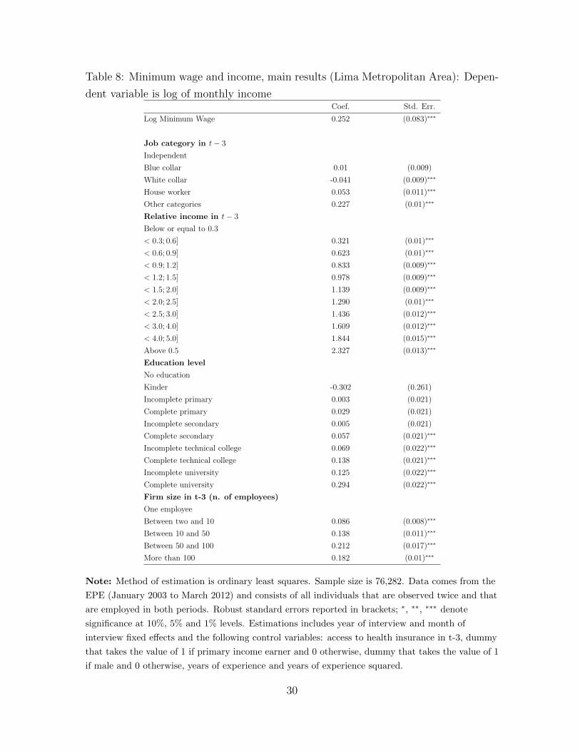
Table 8: Minimum wage and income, main results (Lima Metropolitan Area): Depen-
dent variable is log of monthly incomeCoef. Std. Err.
Log Minimum Wage 0.252 (0.083)∗∗∗
Job category in t− 3
Independent
Blue collar 0.01 (0.009)
White collar -0.041 (0.009)∗∗∗
House worker 0.053 (0.011)∗∗∗
Other categories 0.227 (0.01)∗∗∗
Relative income in t− 3
Below or equal to 0.3
< 0.3; 0.6] 0.321 (0.01)∗∗∗
< 0.6; 0.9] 0.623 (0.01)∗∗∗
< 0.9; 1.2] 0.833 (0.009)∗∗∗
< 1.2; 1.5] 0.978 (0.009)∗∗∗
< 1.5; 2.0] 1.139 (0.009)∗∗∗
< 2.0; 2.5] 1.290 (0.01)∗∗∗
< 2.5; 3.0] 1.436 (0.012)∗∗∗
< 3.0; 4.0] 1.609 (0.012)∗∗∗
< 4.0; 5.0] 1.844 (0.015)∗∗∗
Above 0.5 2.327 (0.013)∗∗∗
Education level
No education
Kinder -0.302 (0.261)
Incomplete primary 0.003 (0.021)
Complete primary 0.029 (0.021)
Incomplete secondary 0.005 (0.021)
Complete secondary 0.057 (0.021)∗∗∗
Incomplete technical college 0.069 (0.022)∗∗∗
Complete technical college 0.138 (0.021)∗∗∗
Incomplete university 0.125 (0.022)∗∗∗
Complete university 0.294 (0.022)∗∗∗
Firm size in t-3 (n. of employees)
One employee
Between two and 10 0.086 (0.008)∗∗∗
Between 10 and 50 0.138 (0.011)∗∗∗
Between 50 and 100 0.212 (0.017)∗∗∗
More than 100 0.182 (0.01)∗∗∗
Note: Method of estimation is ordinary least squares. Sample size is 76,282. Data comes from the
EPE (January 2003 to March 2012) and consists of all individuals that are observed twice and that
are employed in both periods. Robust standard errors reported in brackets; ∗, ∗∗, ∗∗∗ denote
significance at 10%, 5% and 1% levels. Estimations includes year of interview and month of
interview fixed effects and the following control variables: access to health insurance in t-3, dummy
that takes the value of 1 if primary income earner and 0 otherwise, dummy that takes the value of 1
if male and 0 otherwise, years of experience and years of experience squared.
30
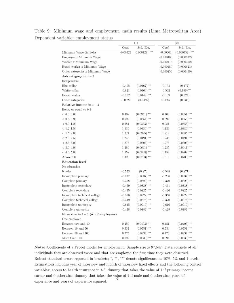
Table 9: Minimum wage and employment, main results (Lima Metropolitan Area)
Dependent variable: employment status(1) (2)
Coef. Std. Err. Coef. Std. Err.
Minimum Wage (in Soles) -0.00324 (0.000729) ∗∗∗ -0.00303 (0.000752) ∗∗∗
Employee x Minimum Wage -0.000486 (0.000332)
Worker x Minimum Wage -0.000116 (0.000372)
House worker x Minimum Wage -0.000180 (0.000623)
Other categories x Minimum Wage -0.000256 (0.000450)
Job category in t− 3
Independent
Blue collar -0.405 (0.0467)∗∗∗ -0.155 (0.177)
White collar -0.621 (0.0464)∗∗∗ -0.562 (0.196)∗∗∗
House worker -0.202 (0.0449)∗∗∗ -0.109 (0.324)
Other categories -0.0622 (0.0489) 0.0687 (0.236)
Relative income in t− 3
Below or equal to 0.3
< 0.3; 0.6] 0.408 (0.0351) ∗∗∗ 0.408 (0.0351)∗∗∗
< 0.6; 0.9] 0.692 (0.0354)∗∗∗ 0.692 (0.0355)∗∗∗
< 0.9; 1.2] 0.981 (0.0353) ∗∗∗ 0.981 (0.0353)∗∗∗
< 1.2; 1.5] 1.139 (0.0380)∗∗∗ 1.139 (0.0380)∗∗∗
< 1.5; 2.0] 1.221 (0.0385) ∗∗∗ 1.219 (0.0385)∗∗∗
< 2.0; 2.5] 1.246 (0.0491)∗∗∗ 1.245 (0.0491)∗∗∗
< 2.5; 3.0] 1.276 (0.0605)∗∗∗ 1.275 (0.0605)∗∗∗
< 3.0; 4.0] 1.286 (0.0641) ∗∗∗ 1.285 (0.0641)∗∗∗
< 4.0; 5.0] 1.158 (0.0868) ∗∗∗ 1.159 (0.0868)∗∗∗
Above 5.0 1.320 (0.0703) ∗∗∗ 1.319 (0.0703)∗∗∗
Education level
No education
Kinder -0.553 (0.870) -0.548 (0.871)
Incomplete primary -0.237 (0.0837)∗∗∗ -0.238 (0.0837)∗∗∗
Complete primary -0.368 (0.0823)∗∗∗ -0.370 (0.0823)∗∗∗
Incomplete secondary -0.459 (0.0838)∗∗∗ -0.461 (0.0838)∗∗∗
Complete secondary -0.435 (0.0825)∗∗∗ -0.436 (0.0825)∗∗∗
Incomplete technical college -0.356 (0.0922)∗∗∗ -0.358 (0.0922)∗∗∗
Complete technical college -0.319 (0.0876)∗∗∗ -0.320 (0.0876)∗∗∗
Incomplete university -0.615 (0.0910)∗∗∗ -0.616 (0.0910)∗∗∗
Complete university -0.438 (0.0889)∗∗∗ -0.439 (0.0889)∗∗∗
Firm size in t− 3 (n. of employees)
One employee
Between two and 10 0.450 (0.0403) ∗∗∗ 0.451 (0.0403)∗∗∗
Between 10 and 50 0.532 (0.0551)∗∗∗ 0.534 (0.0551)∗∗∗
Between 50 and 100 0.775 (0.0934)∗∗∗ 0.776 (0.0934)∗∗∗
More than 100 0.892 (0.0536)∗∗∗ 0.894 (0.0536)∗∗∗
Note: Coefficients of a Probit model for employment. Sample size is 97,547. Data consists of all
individuals that are observed twice and that are employed the first time they were observed.
Robust standard errors reported in brackets; ∗, ∗∗, ∗∗∗ denote significance at 10%, 5% and 1 levels.
Estimations includes year of interview and month of interview fixed effects and the following control
variables: access to health insurance in t-3, dummy that takes the value of 1 if primary income
earner and 0 otherwise, dummy that takes the value of 1 if male and 0 otherwise, years of
experience and years of experience squared.31
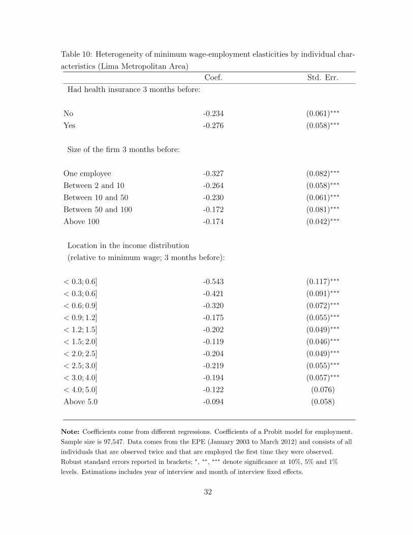
Table 10: Heterogeneity of minimum wage-employment elasticities by individual char-
acteristics (Lima Metropolitan Area)
Coef. Std. Err.
Had health insurance 3 months before:
No -0.234 (0.061)∗∗∗
Yes -0.276 (0.058)∗∗∗
Size of the firm 3 months before:
One employee -0.327 (0.082)∗∗∗
Between 2 and 10 -0.264 (0.058)∗∗∗
Between 10 and 50 -0.230 (0.061)∗∗∗
Between 50 and 100 -0.172 (0.081)∗∗∗
Above 100 -0.174 (0.042)∗∗∗
Location in the income distribution
(relative to minimum wage; 3 months before):
< 0.3; 0.6] -0.543 (0.117)∗∗∗
< 0.3; 0.6] -0.421 (0.091)∗∗∗
< 0.6; 0.9] -0.320 (0.072)∗∗∗
< 0.9; 1.2] -0.175 (0.055)∗∗∗
< 1.2; 1.5] -0.202 (0.049)∗∗∗
< 1.5; 2.0] -0.119 (0.046)∗∗∗
< 2.0; 2.5] -0.204 (0.049)∗∗∗
< 2.5; 3.0] -0.219 (0.055)∗∗∗
< 3.0; 4.0] -0.194 (0.057)∗∗∗
< 4.0; 5.0] -0.122 (0.076)
Above 5.0 -0.094 (0.058)
Note: Coefficients come from different regressions. Coefficients of a Probit model for employment.
Sample size is 97,547. Data comes from the EPE (January 2003 to March 2012) and consists of all
individuals that are observed twice and that are employed the first time they were observed.
Robust standard errors reported in brackets; ∗, ∗∗, ∗∗∗ denote significance at 10%, 5% and 1%
levels. Estimations includes year of interview and month of interview fixed effects.
32
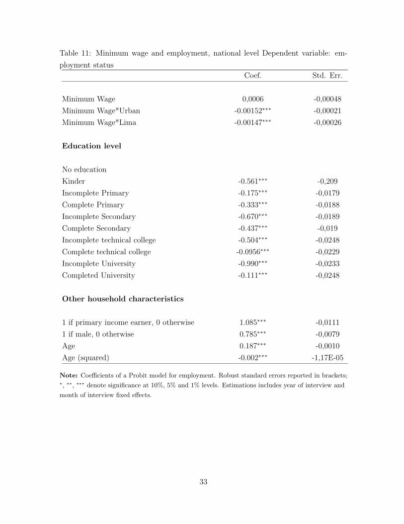
Table 11: Minimum wage and employment, national level Dependent variable: em-
ployment status
Coef. Std. Err.
Minimum Wage 0,0006 -0,00048
Minimum Wage*Urban -0.00152∗∗∗ -0,00021
Minimum Wage*Lima -0.00147∗∗∗ -0,00026
Education level
No education
Kinder -0.561∗∗∗ -0,209
Incomplete Primary -0.175∗∗∗ -0,0179
Complete Primary -0.333∗∗∗ -0,0188
Incomplete Secondary -0.670∗∗∗ -0,0189
Complete Secondary -0.437∗∗∗ -0,019
Incomplete technical college -0.504∗∗∗ -0,0248
Complete technical college -0.0956∗∗∗ -0,0229
Incomplete University -0.990∗∗∗ -0,0233
Completed University -0.111∗∗∗ -0,0248
Other household characteristics
1 if primary income earner, 0 otherwise 1.085∗∗∗ -0,0111
1 if male, 0 otherwise 0.785∗∗∗ -0,0079
Age 0.187∗∗∗ -0,0010
Age (squared) -0.002∗∗∗ -1,17E-05
Note: Coefficients of a Probit model for employment. Robust standard errors reported in brackets;∗, ∗∗, ∗∗∗ denote significance at 10%, 5% and 1% levels. Estimations includes year of interview and
month of interview fixed effects.
33
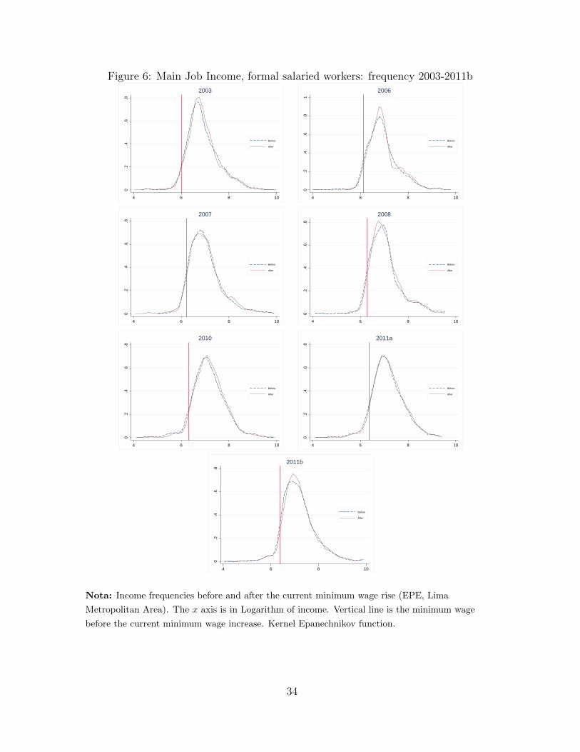
Figure 6: Main Job Income, formal salaried workers: frequency 2003-2011b
0.2
.4.6
.8
4 6 8 10lo g ( in c o m e )
Before
After
2003
0.2
.4.6
.81
4 6 8 10lo g ( in c o m e )
Before
After
2006
0.2
.4.6
.8
4 6 8 10lo g ( in c o m e )
Before
After
2007
0.2
.4.6
.8
4 6 8 10lo g ( in c o m e )
Before
After
2008
0.2
.4.6
.8
4 6 8 10lo g ( in c o m e )
Before
After
2010
0.2
.4.6
.8
4 6 8 10lo g ( in c o m e )
Before
After
2011a
0.2
.4.6
.8
4 6 8 10lo g ( in c o m e )
Before
After
2011b
Nota: Income frequencies before and after the current minimum wage rise (EPE, Lima
Metropolitan Area). The x axis is in Logarithm of income. Vertical line is the minimum wage
before the current minimum wage increase. Kernel Epanechnikov function.
34
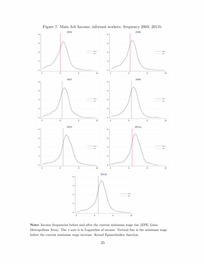
Figure 7: Main Job Income, informal workers: frequency 2003- 2011b
0.2
.4.6
.8
4 6 8 10lo g ( in c o m e )
Before
After
2003
0.2
.4.6
.8
4 6 8 10lo g ( in c o m e )
Before
After
2006
0.2
.4.6
.8
4 6 8 10lo g ( in c o m e )
Before
After
2007
0.2
.4.6
.8
4 6 8 10lo g ( in c o m e )
Before
After
2008
0.2
.4.6
.8
4 6 8 10lo g ( in c o m e )
Before
After
2010
0.2
.4.6
.8
4 6 8 10lo g ( in c o m e )
Before
After
2011a
0.2
.4.6
.8
4 6 8 10lo g ( in c o m e )
Before
After
2011b
Note: Income frequencies before and after the current minimum wage rise (EPE, Lima
Metropolitan Area). The x axis is in Logarithm of income. Vertical line is the minimum wage
before the current minimum wage increase. Kernel Epanechnikov function.
35
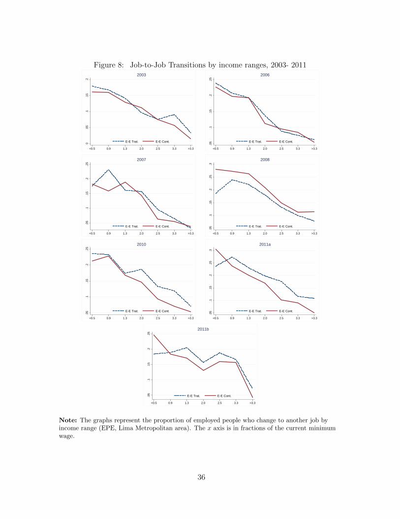
Figure 8: Job-to-Job Transitions by income ranges, 2003- 2011
0.0
5.1
.15
.2
<0.5 0.9 1.3 2.0 2.5 3.3 >3.3R I
E-E Trat. E-E Cont.
2003
.05
.1.1
5.2
.25
<0.5 0.9 1.3 2.0 2.5 3.3 >3.3R I
E-E Trat. E-E Cont.
2006
.05
.1.1
5.2
.25
<0.5 0.9 1.3 2.0 2.5 3.3 >3.3R I
E-E Trat. E-E Cont.
2007
.05
.1.1
5.2
.25
.3
<0.5 0.9 1.3 2.0 2.5 3.3 >3.3R I
E-E Trat. E-E Cont.
2008
.05
.1.1
5.2
.25
<0.5 0.9 1.3 2.0 2.5 3.3 >3.3R I
E-E Trat. E-E Cont.
2010
.05
.1.1
5.2
.25
.3
<0.5 0.9 1.3 2.0 2.5 3.3 >3.3R I
E-E Trat. E-E Cont.
2011a
.05
.1.1
5.2
.25
<0.5 0.9 1.3 2.0 2.5 3.3 >3.3R I
E-E Trat. E-E Cont.
2011b
Note: The graphs represent the proportion of employed people who change to another job byincome range (EPE, Lima Metropolitan area). The x axis is in fractions of the current minimumwage.
36
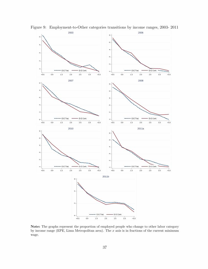
Figure 9: Employment-to-Other categories transitions by income ranges, 2003- 2011
.1.2
.3.4
.5
<0.5 0.9 1.3 2.0 2.5 3.3 >3.3R I
E-E Trat. E-E Cont.
2003
.1.2
.3.4
.5.6
<0.5 0.9 1.3 2.0 2.5 3.3 >3.3R I
E-E Trat. E-E Cont.
2006
0.1
.2.3
.4.5
<0.5 0.9 1.3 2.0 2.5 3.3 >3.3R I
E-E Trat. E-E Cont.
2007
.1.2
.3.4
.5.6
<0.5 0.9 1.3 2.0 2.5 3.3 >3.3R I
E-E Trat. E-E Cont.
2008
.1.2
.3.4
.5.6
<0.5 0.9 1.3 2.0 2.5 3.3 >3.3R I
E-E Trat. E-E Cont.
2010
.1.2
.3.4
.5.6
<0.5 0.9 1.3 2.0 2.5 3.3 >3.3R I
E-E Trat. E-E Cont.
2011a
0.2
.4.6
<0.5 0.9 1.3 2.0 2.5 3.3 >3.3R I
E-E Trat. E-E Cont.
2011b
Note: The graphs represent the proportion of employed people who change to other labor categoryby income range (EPE, Lima Metropolitan area). The x axis is in fractions of the current minimumwage.
37
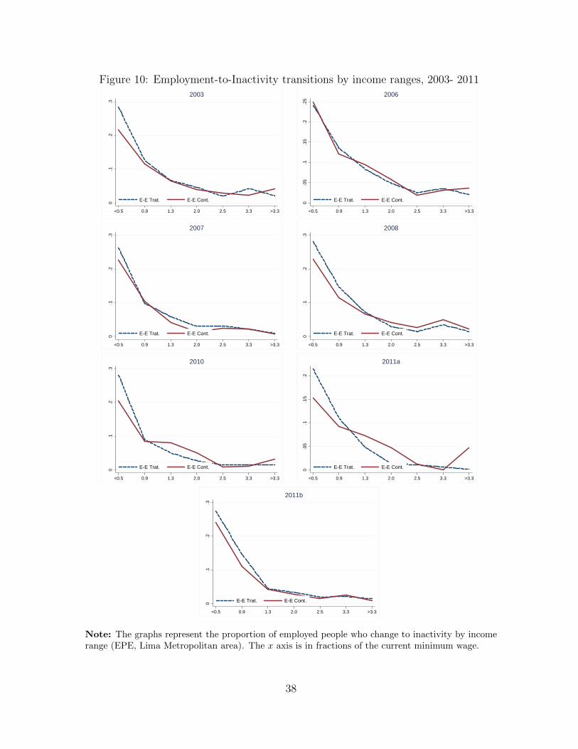
Figure 10: Employment-to-Inactivity transitions by income ranges, 2003- 2011
0.1
.2.3
<0.5 0.9 1.3 2.0 2.5 3.3 >3.3R I
E-E Trat. E-E Cont.
2003
0.0
5.1
.15
.2.2
5
<0.5 0.9 1.3 2.0 2.5 3.3 >3.3R I
E-E Trat. E-E Cont.
2006
0.1
.2.3
<0.5 0.9 1.3 2.0 2.5 3.3 >3.3R I
E-E Trat. E-E Cont.
2007
0.1
.2.3
<0.5 0.9 1.3 2.0 2.5 3.3 >3.3R I
E-E Trat. E-E Cont.
2008
0.1
.2.3
<0.5 0.9 1.3 2.0 2.5 3.3 >3.3R I
E-E Trat. E-E Cont.
2010
0.0
5.1
.15
.2
<0.5 0.9 1.3 2.0 2.5 3.3 >3.3R I
E-E Trat. E-E Cont.
2011a
0.1
.2.3
<0.5 0.9 1.3 2.0 2.5 3.3 >3.3R I
E-E Trat. E-E Cont.
2011b
Note: The graphs represent the proportion of employed people who change to inactivity by incomerange (EPE, Lima Metropolitan area). The x axis is in fractions of the current minimum wage.
38
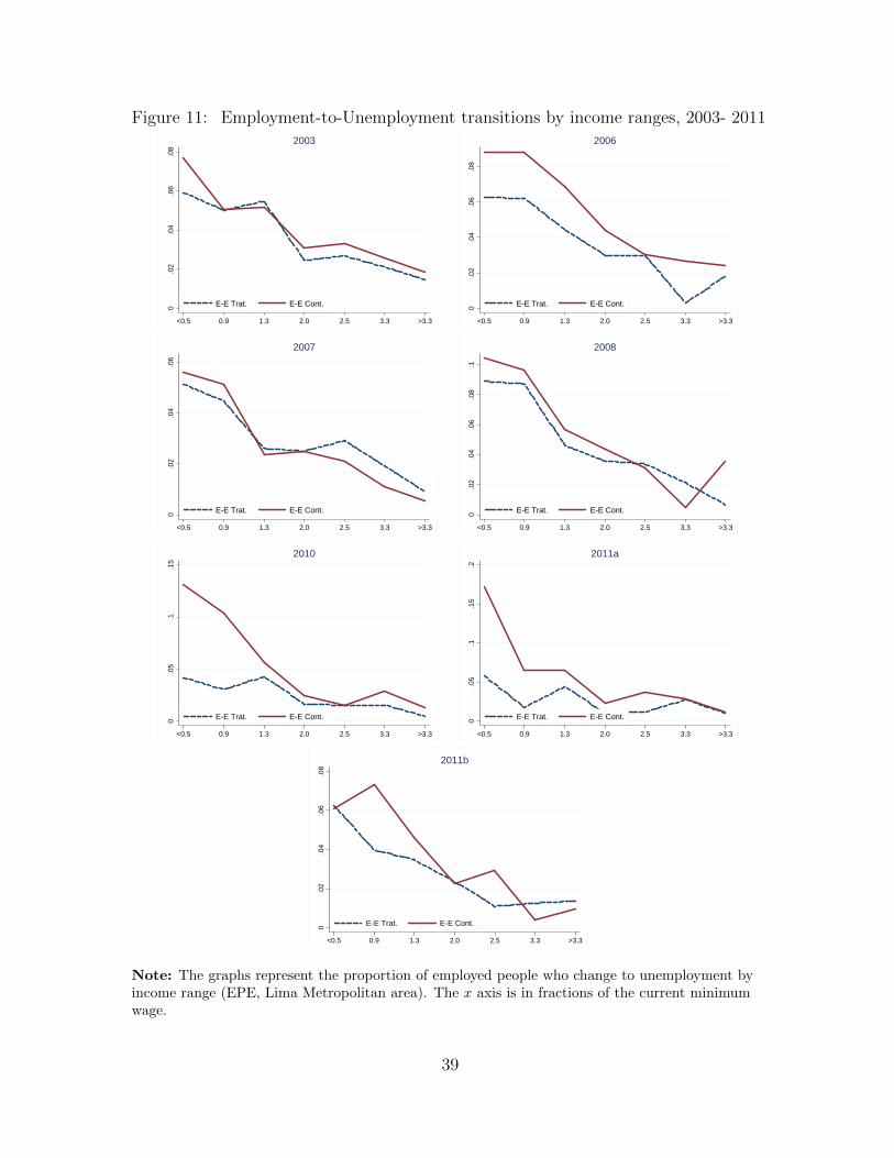
Figure 11: Employment-to-Unemployment transitions by income ranges, 2003- 2011
0.0
2.0
4.0
6.0
8
<0.5 0.9 1.3 2.0 2.5 3.3 >3.3R I
E-E Trat. E-E Cont.
2003
0.0
2.0
4.0
6.0
8
<0.5 0.9 1.3 2.0 2.5 3.3 >3.3R I
E-E Trat. E-E Cont.
2006
0.0
2.0
4.0
6
<0.5 0.9 1.3 2.0 2.5 3.3 >3.3R I
E-E Trat. E-E Cont.
2007
0.0
2.0
4.0
6.0
8.1
<0.5 0.9 1.3 2.0 2.5 3.3 >3.3R I
E-E Trat. E-E Cont.
2008
0.0
5.1
.15
<0.5 0.9 1.3 2.0 2.5 3.3 >3.3R I
E-E Trat. E-E Cont.
2010
0.0
5.1
.15
.2
<0.5 0.9 1.3 2.0 2.5 3.3 >3.3R I
E-E Trat. E-E Cont.
2011a
0.0
2.0
4.0
6.0
8
<0.5 0.9 1.3 2.0 2.5 3.3 >3.3R I
E-E Trat. E-E Cont.
2011b
Note: The graphs represent the proportion of employed people who change to unemployment byincome range (EPE, Lima Metropolitan area). The x axis is in fractions of the current minimumwage.
39
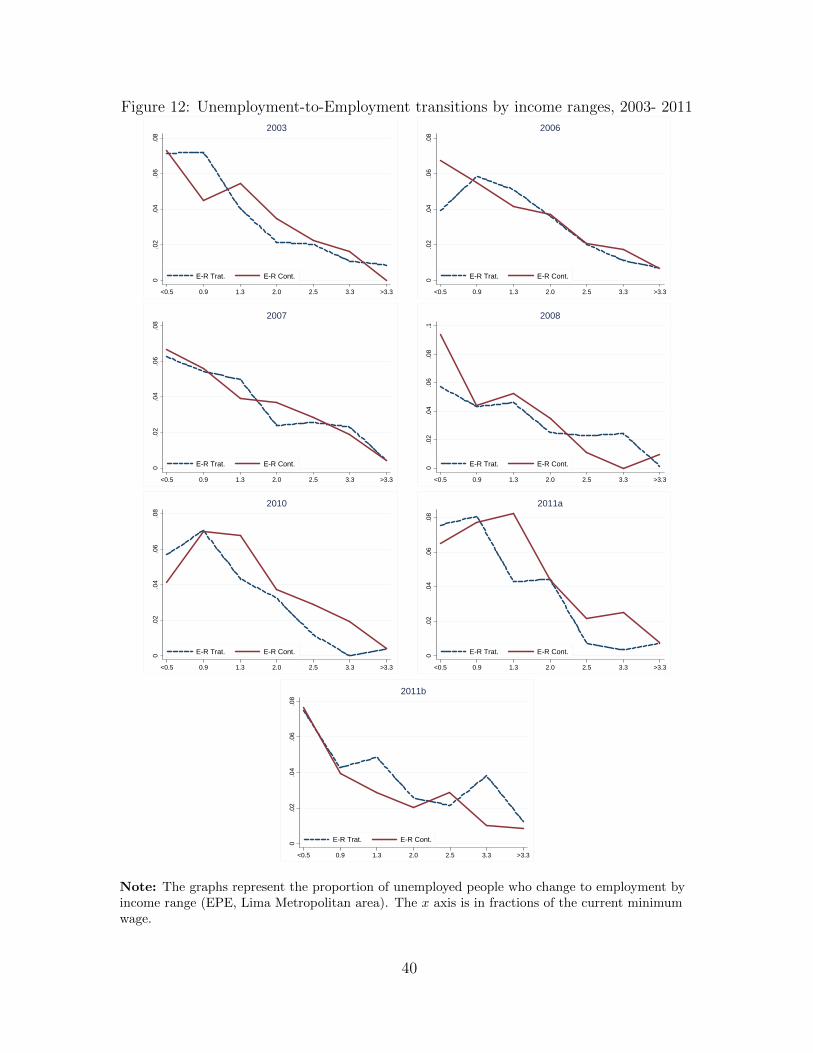
Figure 12: Unemployment-to-Employment transitions by income ranges, 2003- 2011
0.0
2.0
4.0
6.0
8
<0.5 0.9 1.3 2.0 2.5 3.3 >3.3R I 2
E-R Trat. E-R Cont.
2003
0.0
2.0
4.0
6.0
8
<0.5 0.9 1.3 2.0 2.5 3.3 >3.3R I 2
E-R Trat. E-R Cont.
2006
0.0
2.0
4.0
6.0
8
<0.5 0.9 1.3 2.0 2.5 3.3 >3.3R I 2
E-R Trat. E-R Cont.
2007
0.0
2.0
4.0
6.0
8.1
<0.5 0.9 1.3 2.0 2.5 3.3 >3.3R I 2
E-R Trat. E-R Cont.
2008
0.0
2.0
4.0
6.0
8
<0.5 0.9 1.3 2.0 2.5 3.3 >3.3R I 2
E-R Trat. E-R Cont.
2010
0.0
2.0
4.0
6.0
8
<0.5 0.9 1.3 2.0 2.5 3.3 >3.3R I 2
E-R Trat. E-R Cont.
2011a
0.0
2.0
4.0
6.0
8
<0.5 0.9 1.3 2.0 2.5 3.3 >3.3R I 2
E-R Trat. E-R Cont.
2011b
Note: The graphs represent the proportion of unemployed people who change to employment byincome range (EPE, Lima Metropolitan area). The x axis is in fractions of the current minimumwage.
40
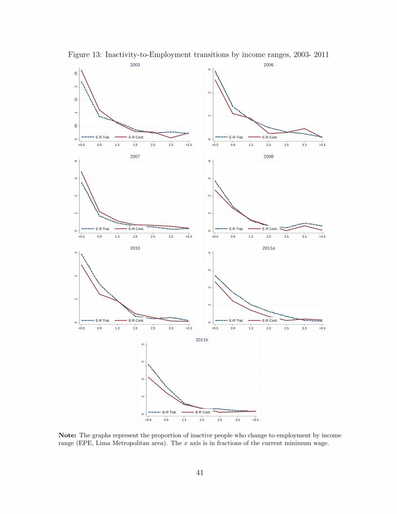
Figure 13: Inactivity-to-Employment transitions by income ranges, 2003- 2011
0.0
5.1
.15
.2.2
5
<0.5 0.9 1.3 2.0 2.5 3.3 >3.3R I 2
E-R Trat. E-R Cont.
2003
0.1
.2.3
<0.5 0.9 1.3 2.0 2.5 3.3 >3.3R I 2
E-R Trat. E-R Cont.
2006
0.1
.2.3
.4
<0.5 0.9 1.3 2.0 2.5 3.3 >3.3R I 2
E-R Trat. E-R Cont.
2007
0.1
.2.3
.4
<0.5 0.9 1.3 2.0 2.5 3.3 >3.3R I 2
E-R Trat. E-R Cont.
2008
0.1
.2.3
<0.5 0.9 1.3 2.0 2.5 3.3 >3.3R I 2
E-R Trat. E-R Cont.
2010
0.1
.2.3
.4
<0.5 0.9 1.3 2.0 2.5 3.3 >3.3R I 2
E-R Trat. E-R Cont.
2011a
0.1
.2.3
.4
<0.5 0.9 1.3 2.0 2.5 3.3 >3.3R I 2
E-R Trat. E-R Cont.
2011b
Note: The graphs represent the proportion of inactive people who change to employment by incomerange (EPE, Lima Metropolitan area). The x axis is in fractions of the current minimum wage.
41